A fast response surface-wave slope meter and measured wind-wave moments

Deep-Sea Research. 1977, Vol. 24, pp. 1211 to 1223. Pergamon Press. Printed in Great Britain.

I N S T R U M E N T S A N D M E T H O D S

A fast response surface-wave slope meter and measured wind-wave moments

B. A. H U G H E S , * H. L. GRANT* and R. W. CHAPPELL*

(Received 2 February 1977: in revised fi~rm 2 May 1977; accepted 10 May 1977)

Abstract Optical, television, and digital electronic techniques are combined in the design of a fast response instrument for the measurement of sea surface slope. Slope is sensed by the refraction of a laser beam, which is detected by a modified television camera. The data rate is reduced to a manageable scale by digital logic, which produces an output directly related to slope. Detailed corrections are applied later by a general purpose computer. The method is designed to be insensitive to variations in the height or curvature of the water surface.

Moments of measured wind-wave slope distribution have been determined for nine data samples and compared with the earlier measurements by Cox and Munk. Agreement is substantial.

I N T R O D U C T I O N

SEVERAL techniques exist for measuring sea-surface wave slopes: the glitter method described by Cox and MUNK (1954a, b), used primarily for determining average slope statistics; the Fourier transform method of STILWELe (1969, see also SUGIMORI, 1975), used mainly for estimating slope wavenumber spectra; the local slope measuring methods of TOBER, ANDERSON and SHEMDIN (1973), STURM and SORRELL (1973, and SCOTT, 1974), used for obtaining time series of slope components at a point ; etc. The instrument we shall describe herein is a 'local-slope' measurer, and the refraction of a narrow light beam emerging from the water surface is its basic operating principle. The devices reported in the previous three references use the same principle, but we implement it differently.

Our device is insensitive to intensity variations of the emergent beam over fairly wide limits, and it is this property, along with its use in sheltered ocean waters, rather than in tanks, that we believe make it worthy of attention. We have devoted considerable effort to understanding the effect of intensity variations (outside the acceptable range of the device) and our conclusion is that the mean square slope of a wind wave field can be measured with less than 15~o error for winds speeds up to 8 m s - 1 ( 16 knots)5- We have also determined the wind dependence of the second-, third-, and fourth-order statistical moments of the slope field, and our results compare favourably with the data of Cox and MUNK (1954b).

PRINCIPLE OF OPERATION

A schematic diagram of the wave slope meter is shown in Fig. 1 and a photograph in Fig. 2. It was designed to be suspended from a crane, 10 m ahead of the bow of a research vessel, and to accommodate wave heights up to about 0.8 m. In use the crane also supports a vertical array of current meters directly below the wave slope meter, and the design of the suspension is such that the wave-slope meter cannot rotate about a vertical axis.

* Defence Research Establishment Pacific. Forces Mail Office, Victoria, B.C., Canada VOS IBO. ? 1 knot = 1 .85kmh -1.

1211

1212 B.A. HUGHES, H. L. GRANT and R. W. CHAPPELL

Fig. 1. Sketch of the wave slope meter. The distance from the top of the laser case to the large simple lens is approximately 1 m.

A laser beam is directed vertically upward through the water surface and, after refraction, it passes through a large lens and falls on a translucent screen placed at the focal plane of the lens. If the lens were perfect, the location of the spot on the screen would depend only on the slope of the water surface, as shown in Fig. 3, and, in particular, not on the water height. The screen is viewed by a television camera, and fast digital circuitry is used to determine the x and y coordinates of the spot in each frame. Subsequent processing of these numbers provides the two components of slope as time series.

~= ~11 ~ FOCAL PLANE

~ ~ - -----)-SUR~CE AT

~-----J-I tiGHT eEAM// DIFFERENT HEIGHTS

Fig. 3. Principle of separation of water height and water slope effects. For a given water slope, but varying water heights, the light beam produces a spot at a fixed location in the focal plane.

TV CAMERA HOUSING

SUN ~-SHADE

LARGE LENS

S LASER

HOUSING

CURRENT METERS

Fig. 2. Wave slope meter (not in situ) and part of the lower current meier array.

[facing p. 1212]

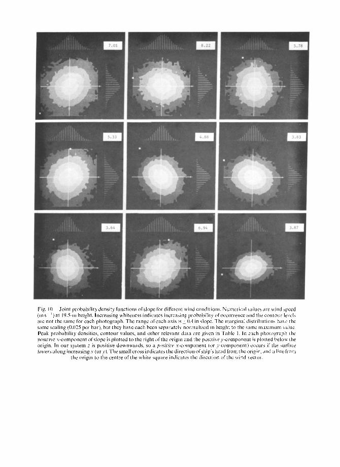
Fig. 10. Joint probability density functions of slope for different wind conditions. Numerical wdues are wind speed [m s ~} at 19.5-m height. Increasing whiteness indicates increasing probability of occurrence and the contour levels are not the same for each photograph. The range o[each axis is _+ 0.4 in slope. The marginal distributions have the same scaling (0.025 per bar), but they have each been separately normalized in height to the same maximum value. Peak probability densities, contour values, and other relevant data are given in Table 1. In each photograph the positive x-component of slope is plotted to the right of the origin and the positive y-component is plotted belov,, tile origin. In our system z is positive downwards, so a pe~sitice x-component lot ) '-component} occurs if the surface lmrers along increasing x (or 3'). The small cross indicates the direction of ship's head from the origin, and a line from

the origin to the centre of the white square indicates the direction of the wind vector.

A fast response surface-wave slope meter and measured wind-wave moments 1213

O PI ICAL E Q U I P M E N T

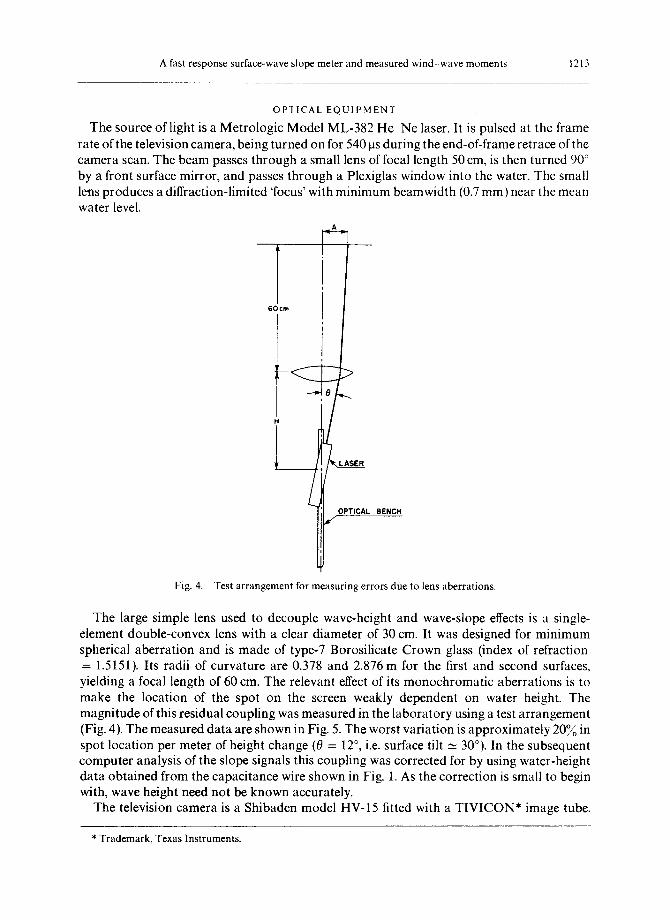
The source of light is a Metrologic Model ML-382 H e - N e laser. It is pulsed at the frame rate of the television camera, being turned on for 540 its during the end-of-frame retrace of the camera scan. The beam passes through a small lens of focal length 50 cm, is then turned 90 ° by a front surface mirror, and passes through a Plexiglas window into the water. The small lens produces a diffraction-limited 'focus' with minimum beamwidth (0.7 mm) near the mean water level.

60 cm

H

~1~ LASER

Z OPTICAL BENCH

7

Fig. 4. Test arrangement for measuring errors due to lens aberrations.

The large simple lens used to decouple wave-height and wave-slope effects is a single- element double-convex lens with a clear diameter of 30 cm. It was designed for minimum spherical aberration and is made of type-7 Borosilicate Crown glass (index of refraction = 1.5151). Its radii of curvature are 0.378 and 2.876m for the first and second surfaces, yielding a focal length of 60 cm. The relevant effect of its monochromatic aberrations is to make the location of the spot on the screen weakly dependent on water height. The magnitude of this residual coupling was measured in the laboratory using a test arrangement (Fig. 4). The measured data are shown in Fig. 5. The worst variation is approximately 20?/0 in spot location per meter of height change (0 = 12 °, i.e. surface tilt ~ 30°). In the subsequent computer analysis of the slope signals this coupling was corrected for by using water-height data obtained from the capacitance wire shown in Fig. 1. As the correction is small to begin with, wave height need not be known accurately.

The television camera is a Shibaden model HV-15 fitted with a T I V I C O N * image tube.

* Trademark, Texas Instruments.

1214 B.A. HUGHES, I . | . L. GRANT and R. W. CHAPPELL

This tube differs from a normal vidicon in that it uses a silicon-diode array rather than a photoconductive film. The principal advantage for this application is that the lag is considerably less than for the usual vidicon. ('Lag' is the percentage of the charge pattern that remains on the target after it is scanned by the electron beam.) The c~tmera was modified to remove the interlace scan, reduce the vertical resolution from 525 lines to l l 1 lines, and increase the frame rate to 112.47 frames s-1. The last number happens to be a convenient sub-multiple of the clock frequency available in the camera. The tube is operated with a

~ig. 5.

I0

o

°. o

w l-- hl Z~ ~o

g o

8=2 °

I I I ,~o o..,o o . .o o.eo , !oo ' ,! , ,o 1.20

H (HETEflS)

The effects of aberrations in the large lens as measured with the test setup of Fig. 4. In the absence of aberrations, A would be independent of H.

target voltage of 40 V (while data are being recorded) and this is four times the maximum value recommended by the manufacturer. Although the lag is significantly reduced by this means, we have had a tube failure, perhaps because of this treatment.

An interference filter, 100 A wide and centred at the laser wavelength, is situated in front of the camera lens. This allows the instrument to be used in the daylight provided that no sun 'glints' are falling on the screen within the field of view of the TV camera. This difficulty is partially overcome by the cloth sunshade around the lens (Fig. 2), but under conditions of low sun and rough water an occasional flash of sunlight gets into the system and such data have to be discarded.


SHIPBOARD SIGNAL PROCESSOR

The purpose of this device is to examine each frame of the output of the TV camera, decide if it contains an acceptable spot, if it does, determine the location of its "centre' according to certain rules, and put out two D.C. voltages representing the x and y coordinates of the centre of the spot, the x direction being parallel to a scan line. The D.C. voltages are derived from the horizontal (x) and vertical (y) sweep signals. There are 1 l 1 lines in each frame and each line is divided into 128 equal segments with lengths equal to the line spacing. This produces equal resolution in x and y. The video signal from each of the 128 × 111 line segments is compared sequentially to a D.C. threshold voltage. The x coordinate of each segment for which the signal exceeds the threshold is fed to an averaging circuit which produces a simple equal- weight average of all such x values over the whole frame. Another averaging circuit computes the equal-weight average of the y coordinate of all lines that contain a signal above the threshold. These two values, which we take as our definition of the "centre' of the spot, are then recorded.

There are two controls on this instrument, the threshold voltage level and a remote control for the television camera f-number. Both need to be adjusted from time to time, primarily to correct for average intensity changes of the beam as the average roughness of the sea surface changes with changing wind conditions. In fact, intensity of the spot on the translucent screen depends instantaneously on the local curvature of the water surface, and thus for a random sea surface it fluctuates considerably. To facilitate proper operation of these controls, automatic monitoring circuits are included to check each frame and provide visual indications (flashing lights) when either of two abnormal conditions exist: no spot is detected, or more than one identifiable spot is detected. The procedure that we use at sea is to adjust each control until (a) neither abnormal condition is indicated (exactly one spot detected per frame), or more usually, (b) both abnormalities occur with approximately equal frequency (both lights flash at the same rate). If the threshold level is set too high, spots will not be detected in some frames. In that case, the output coordinates of the previous frame are held. If the threshold is too low, the lag spot from one or more previous frames will be detected. In this case values from the previous frames will be erroneously included in the average that produces the coordinates for the present frame. The camera stop needs to be opened on windy days when the average curvature is large and the spot intensity tends to approach the noise level of the camera. On calm days the aperture must be reduced to prevent serious overloading of the camera. Only on nearly calm days is it possible to set the controls so that one and only one spot is detected in each frame.

The intensity of the laser beam can vary over a wide range before errors occur in the x and y output values. The camera tube has a transfer characteristic with ~ = 1 [slope of log (intensity) versus log (video signal current)], and a usable intensity range of 18 dB (65:1) between saturation and dark current, for a fixed f-number. By using the video signal only as a simple on-off indicator (when compared with the threshold value), the dynamic range of the instrument is changed somewhat from 18 dB; in fact, the useful intensity range is extended beyond saturation into the region of moderate 'blooming', but, of course, the range at the low-intensity end is reduced. From published curves (The opto-electronics data book, Texas Instruments, First Edition, p. 311 and following) we estimate that the extension at high intensities is 10 to 20 dB ; the loss at the low end depends directly on the threshold value used and thus varies with the encountered operating conditions. The overall effect of non-zero threshold values (and non-fixed f-number) is described in some detail in the next section.


FURTHER CONSIDERATIONS OF ABNORMAL CONDITIONS

The no-spot condit ion has three causes: (a) curvature, which makes the spot too weak to be detected, (b) a slope so large that the beam misses the large lens or the scanned part of the screen, or (c) foam or flotsam on the water surface interfering with or extinguishing the beam. All of these situations result in successive output points with identical pairs of (x, y) values, so that the occurrence of missing spots can be studied by examining data f rom the instrument. We made such an examinat ion of a data set consisting of 50 time series recorded in July 1972 in Bute Inlet and the Strait of Georgia on the west coast of Canada.* Firstly, we determined the fraction of each series that possessed successively identical x-values and simultaneously

Q

t_)

I - - Z O t0 .10 c:a& u--0 t~l ;

) . - - . I i ,-.I o

Z a a

o 0, a o

I ' - Z I .~1o

f r o

o o O o °°l

• ' °

. . . . . . . . . . . . . . cr' . . . . . . . 0 - '

Ta'I'RL MERN-SI]I.IARE 'SLOPE '

Fig. 6. Percentage of data abnormally identical ( ~ °/o no-spot frames) as a function of the mean-square slope. The average value is 9.7~o and there is no significant trend with roughness. The measurements were made in Bute ]inlet

and Georgia Strait in 1972 and each point represents a different wind speed (range. very light to 8 m s- ~ ).

identical y-values. Then we estimated the fraction that would be 'proper ly ' identical in each series, and, by subtract ing this from the measured values, we obtained an estimate of the fraction of each series that was ' abnormal ly ' identical ; i.e. an estimate of the fraction of each series that had no-spot frames. Estimates of the 'proper ly ' identical fraction were based on simple probabilistic arguments applied to r a n d o m Gaussian signals that had variances and autocorrelat ions at a lag of one point equal to the real signals. This simple model predicted accurately the percentage of identical successive values in computer-generated r andom test signals.

For the full fifty-series data set, the estimated fraction of 'no-spot ' frames is illustrated in Fig. 6. The x-axis in this figure represents logari thmic values of total mean-square 'slope', i.e. the sums of variances of the x and y slope signals including those from the 'no-spot ' frames. The percentage of no-spot frames appears to be basically independent of mean-square output (implying perhaps that curvature is statistically independent of slope). Some of the scatter in the ordinate values as illustrated will be due to finite-length statistical variations in the

* For a further description of these time series, see HUGHES and GRANT (tO be published), and HuRriEs (to be puhlished).


'properly' identical fraction. Our simple probabilistic model used infinite sample length arguments. We also believe that this accounts for the one 'impossible' negative percentage. The total range in ordinate values is from - 3 to 23.6% and the average value is 9.7'~o.

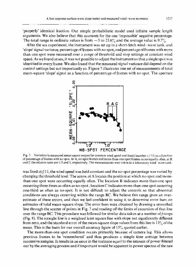
After the sea experiment, the instrument was set up in a short-fetch wind-wave tank, and 'slope' signal variance, percentage of frames with no spot, and percentage of frames with more than one spot were measured over a range of threshold and stop settings at constant wind speed. As we found at sea, it was not possible to adjust the instrument so that a single spot was identified in every frame. We also found that the measured signal variance did depend on the control settings but not importantly so. Figure 7 illustrates one set of measurements of total mean-square 'slope' signal as a function of percentage of frames with no spot. The aperture

.~_ BAC

NO-SPOT FEBCENTFIGE Fig. 7. Variation in measured mean square output for constant wind speed and fixed/~number (.1/11 ) as a function of percentage of frames with no spot. At A, no-spot frames and more-than-one-spot frames occur equally often, at B and C the relative rates are 1/3 and 3, respectively. The measurements were taken in a laboratory wind wave tank.

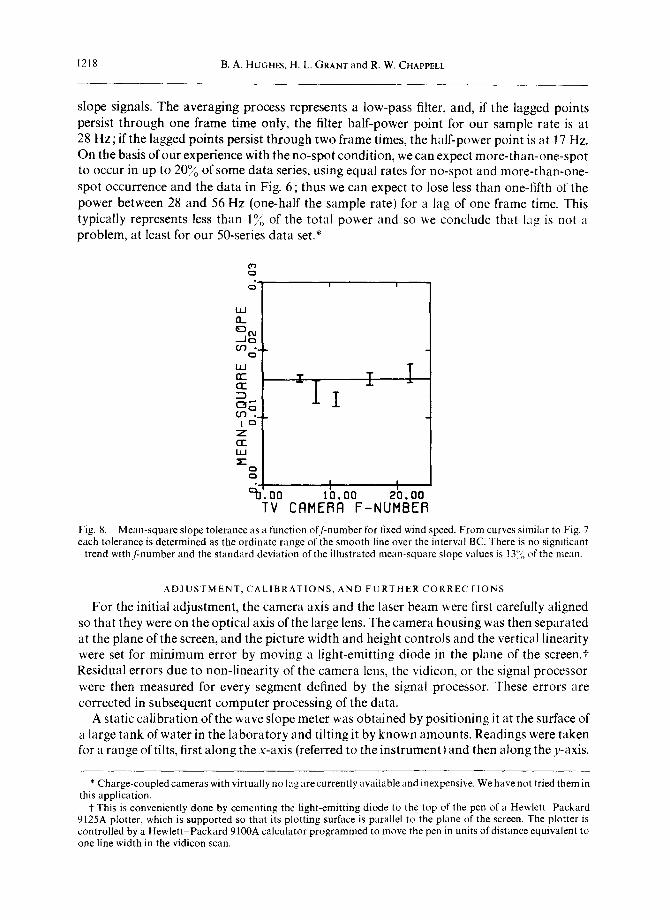
was fixed at f/11, the wind speed was held constant and the no-spot percentage was varied by changing the threshold level. The arrow at A locates the position at which no-spot and more- than-one spot were occurring equally often. The location B indicates more-than-one spot occurring three times as often as no-spot ; location C indicates more-than-one spot occurring one-third as often as no-spot. It is not difficult to adjust the controls so that abnormal conditions are always occurring within the range BC. We believe this range gives an over- estimate of these errors, and thus we feel confident in using it to determine error bars on estimates of total mean-square slope. The error bars were obtained by drawing a smoothed line through the scatter of points in Fig. 7 and reading offthe limits of excursion of that line over the range BC. This procedure was followed for similar data taken at a number o f f stops (Fig. 8). The straight line is a weighted least square line with slope not significantly different from zero, and the standard error of the mean-square slope values from this line is 13~o of the mean. This is the basis for our overall accuracy figure of 15~o quoted earlier.

The more-than-one spot condition occurs primarily because of camera lag. This allows previous frames to be 'remembered' and thus produces a simple time average between successive samples. It results in an error in the variance equal to the amount of power filtered out by the averaging process and if important would be apparent in power spectra of the raw


slope signals. The averaging process represents a low-pass filter, and, if the lagged points persist through one frame time only, the filter half-power point for our sample rate is at 28 Hz ; if the lagged points persist through two frame times, the half-power point is at 17 Hz. On the basis of our experience with the no-spot condition, we can expect more-than-one-spot to occur in up to 20~o of some data series, using equal rates for no-spot and more-than-one- spot occurrence and the data in Fig. 6 ; thus we can expect to lose less than one-fifth of the power between 28 and 56 Hz (one-half the sample rate) for a lag of one frame time. This typically represents less than 1~,, of the total power and so we conclude that lag is not a problem, at least for our 50-series data set.*

C~

c~

LU O_

ooc;- i , i OE C~

Z

CE I , i

C~ C~

.00 TV

i i I I I

I I 10,00 20.00

CAMERA F-NUMBER Fig. 8. Mean-square slope tolerance as a function o f f number for tixed wind speed. From curves similar to Fig. 7 each tolerance is determined as the ordinate range of the smooth line over the interwd BC. There is no significant

trend withJ :number and the s tandard deviation of the illustrated mean-square slope wdues is 13% 0 of the mean

A D J U S T M E N T , C AL IB R AT IONS , AND F U R T H E R C O R R E C T I O N S

For the initial adjustment, the camera axis and the laser beam were tirst carefully aligned so that they were on the optical axis of the large lens. The camera housing was then separated at the plane of the screen, and the picture width and height controls and the vertical linearity were set for minimum error by moving a light-emitting diode in the plane of the screen.+ Residual errors due to non-linearity of the camera lens, the vidicon, or the signal processor were then measured for every segment defined by the signal processor. These errors are corrected in subsequent computer processing of the data.

A static calibration of the wave slope meter was obtained by positioning it at the surface of a large tank of water in the laboratory and tilting it by known amounts. Readings were taken for a range of tilts, first along the x-axis (referred to the instrument) and then along the y-axis.

* Charge-coupled cameras with virtually no lag are currently available and inexpensive. We have not tried them in this application.

t This is conveniently done by cementing the light-emitting diode to the top of the pen of a Hewlett Packard 9125A plotter, which is supported so that its plotting surface is parallel to the plane of the screen. The plotter is controlled by a Hewlet t -Packard 9100A calculator programmed to move the pen in units of distance equivalent to one line width in the vidicon scan.


Two gravity-sensitive accelerometers, clamped to the lens case in perpendicular directions, were used to measure the amount of tilt. Distance from the water surface to the lower lens face was also measured. After making the above corrections and those for lens aberrations, the results shown in Fig. 9 were obtained. Between slope values of _+ 0.4 the x-component values have a correlation of 0.9997 and a regression slope of 0.9952, the y-component values have a correlation of 0.9990 and a slope of 1.003. In analyzing our field data, we have chosen to omit all slope values that occur outside this range because non-linearities become important. The effect of this omission is discussed in the next section.

Fig. 9.

6-30. / / / . / / ' / / d '

;7 /

2

-30* --6

r /

--6 - ' 2 '2 "6 WAVE SLOPE METER OUTPUT

Static calibration results for the wave slope meter. S x and Sy are the x and y components of slope.

Auxiliary measurements of wave height are made, principally to permit a correction for lens aberrations. For this purpose, random height errors of as much as 10cm are not expected to have important effects on the measured slope distribution. The sensor is an anodized tantalum wire 0.635mm in diameter and l m long, with a capacitance of 4.6 ~tF m - ~ to the water. The wire is anodized at 80V in seawater, and the anodizing voltage is maintained during operation so that any damage to the dielectric oxide is self-healing. Superimposed on the D.C. anodizing voltage is a 200-Hz carrier frequency maintained at constant voltage at the input to the cable. At this frequency the capacitive reactance betx~ een the wire and the water is much larger than the resistance of the cable and the resistance of the part of the tantalum wire that is in the air, so the current flowing to the wire is a measure of the capacitance and hence the height of the water. The ground is through the aluminum frame.

This device has at least as many troubles as other capacitance wave gauges, but with the low accuracy and limited frequency response required for this application the performance is adequate. As used, the wire is not quite vertical and its angle with the vertical depends on ship speed. Appropriate corrections are made using mean data obtained from the wave slope meter.

WIND SPEED%

(m/s

@

19.5

m)

FRICTION

std.dav.

VKLOCITY

mea

n (%

of

mea

n)

u,

(am

/s)

7.01

12.2

23.7

8.22

8.9

28.9

5.78

10.5

18

.7

5.33

6.1

16.9

4.~8

7.

8 15

.1

3.83

12.8

11.2

3.64

9.5

10.6

6.94

10.3

23

.4

3.87

10.9

10.7

Tab

le

l.

WIND DIRECTION*

mean

s td

. da

y.

(deg

) (d

eg)

138,

5 7.0

196.3

4.4

247.4

4.9

273.5

4.7

233.8

4.5

210.

9 6.

4

243.7

6.2

287.6

5.4

168.0

8.5

Dam

v¢l

lues

f~m

e~l

ch s

et i

n Fi

~]. 1

0.

DISTRIBUTION

SHIP'S

DIRECTION**

FETCH%%

AVERAGING

SPEED

2 a2

(deg

) (km)

TIME(sec)

(m/s)

~c

u

3.4

4.82

767

.65

.0117

.0157

-8.1

5.99

346

.54

.0123

.0178

~16.1

15.7

417

.68

.0121

.0149

41.3

16.1

826

.67

.0135

.0170

-6.9

7.65

737

.61

.0072

.0108

-11.4

77.5

1187

.62

.0061

.0101

13.2

4.08

498

.46

.0076

,0097

38.5

8.25

439

.57

.0134

.0220

-2.8

7.93

310

.69

.0049

.0092

CONTOUR LEVELS

% of peak probability

de=city

jpdf PEAK PROBABILITY

DENSITY VALUES

marginal

marginal

horiz,

vert

.

15.4

3.76

3.77

14.1

3.89

3.29

15.0

3.54

3.75

12.5

3.45

3.46

21.6

4.50

4.56

24.2

5.24

4.36

22.4

4.32

4.81

ii,3

3.10

3.06

32.2

5.71

4.40

44.1

15.4

3.48

.286

48.0

18.6

4.92

.529

46.8

17.6

4.47

.485

46.6

17.4

4.36

.438

42.5

14.1

3.00

.236

34.6

8,80 1.29

.066

39.6

12.0

2,24

.147

52.5

22.9

7.13

1.00

45.3

16.4

3.94

.404

* D

irec

tion

of

win

d ve

ctor

mea

sure

d c

lock

wis

e fr

om

sh

ip's

hea

d.

* *

Mea

sure

d cl

ockw

ise

from

the

rec

ipro

cal

win

d ve

ctor

. T

hes

e va

lues

are

the

dif

l'ere

nces

in

ori

enta

tio

n a

ngle

bet

wee

n o

ur

refe

renc

e fr

ames

and

the

win

d-o

rien

ted

fram

es d

efin

ed a

nd u

sed

by C

ox

and

MU

NK

(t9

54b)

. )

Win

d sp

eed

was

mea

sure

d at

tw

o he

ight

s, 2

1.7

and

8.9

m.

Win

d sp

eed,

U,

at

19.5

m a

nd

fri

ctio

n ve

loci

ty,

,.,

wer

e ca

lcul

ated

as

sum

ing

the

lo

gar

ith

mic

pro

file

U

=

10.0

5 (u

./0.

4t 4

1:s

+(t

~./O

.4)l

n(z/

lO),

w

her

e z

is h

eigh

t an

d t

he u

nit

s ar

e m

eter

s an

d m

eter

s s-

*. T

his

fo

rmu

la w

as o

bta

ined

fro

m W

u (

1969

) an

d it

sat

isfa

ctor

ily

pred

icts

mea

n w

ind

spee

d at

one

mea

sure

men

t he

ight

in

term

s o

f th

e ot

her.

Fo

r al

l da

ta

sets

tile

di

ffer

ence

bet

wee

n ai

r an

d s

urfa

ce w

ater

tem

per

atu

res

(~,-

tw)

rang

e fr

om +

1 to

+ 1

0"C

. +

+ D

ista

nce

to n

eare

st s

hore

, m

easu

red

upw

ind.

All

bu

t on

e se

t w

ere

mea

sure

d i

n a

nar

row

cha

nnel

wit

h m

ou

nta

ino

us

side

s ty

pica

lly

2000

m h

igh

(But

e In

let)

.

.>

;g

C 22

.r-

>

Z

,-}

>


SEA SLOPE M E A S U R E M E N T S

As an example of oceanographic results obtained with the fully corrected, properly adjusted instrument, we present joint probability densities of wind waves taken from the Bute Inlet-Georgia Strait data set. The original measurement series was designed primarily to determine the effect of internal waves on wind waves ; however, we were able to select nine samples recorded at times when there was little or no internal wave activity. Each of these samples is at least 5 rain long and has an r.m.s, wind fluctuation of less than 15'#0 of the mean wind. We consider these nine, therefore, to be unperturbed wind-wave series and have analyzed them as such.

Our results are in Fig. 10 and 11 and Tables 1 and 2. In Fig. 10 we show joint probability density contours of slope for each of the nine data series. Increasing whiteness represents increasing probability of occurrence, the small + sign indicates the direction of ship's head, the wind is blowing from the origin to the centre of the small square and the separations between bars in the marginal distributions are 0.025 in slope. Further details are given in the caption.

We have calculated second-, third-, and fourth-order moments for each of these pdf wflues. By rotating these an appropriate amount we have determined variances cross-wind (or 2), along wind (a~), total (a~ + a,z), and the Gram-Charl ier coefficients for the third- and

Table 2. Wind dependence of moments compared with Cox and Munk 'clean surjace" results. For each coe[ficient the underlined values are statistically dif[erent between sets with at least 99°~o eonJidence. 7he re qression values were obtained assuminq no error in wind speed and using unwei~.lhed moment values. "lT~e wind speed W refers to 19.5-m hei~tht

and both sets ~( data hat,e been adjusted to this hei~tht.

Present Results

A ~

Cox and Munk (19545) 'clean surface'

2 o c .00080 + .00165 W +.002, r = .79 .0029 + .00182 W ~.002, r = .96

2 o u .0015 + .00229 W ~.002, r = .84 .00084 + .00292 W ~.004, r = .96

Oc+a u 2 2 .0023 + .00394 W _+'004, r = .83 .0037 + .00474 W _+.005, r = .97

C03 .224 - .039 W ~.06, r = -.71 .04 - .032 W ~.12, (r not available)

C12 .016 + .024 0

C21 .0086 + .03 .01 - .0083 W ~.03, (r not available)

C30 .030 + .05 0

C04 .40 + .15 .23 + .41

C13 .008 + .03 0

C22 .15 + .08 .12 + ,06

C31 .031 + .059 0

C40 .51 + .29 .40 + .23


t=~

'-z,~

C~ Z

o

h i 0--

( n O ,, IL l O

. ~ . G~

xX

x

e o x

x

e °

x x

x

X X

x

X

X. X

X

I I O0 S .O0 1 0 . 0 0

W I N D S P E E D M / $ R T 1 9 . !

X •

I P O

Q

0

~ '

!

~o X

WIND

X

X

X

X " X

X

1 5 . 0 0 M

°°

0o I l l o

o

wc~" t ~ Q~

I . Z ~ a~ h i

xx

x

xx x

x Xx x x .

x .:.

• O...:.....i:i::::i:ii!i:.::::!ii:?:::

. . . . . . c~ - - <4.. '

I t OO 5 . 0 0 l O . O 0 1 5 . 0 0

WIN[ SPEED H/5 RT 19.5 M

=;" n- Lid p- X x bJ o

~ a , x

Q,.

. T I K e ' r

oo o

':'o:oo WIN0

x ~ x e X

x ; • x x

# x j xx

• x

• • x x x

• x

,!oo ,k.oo .oo ,!00 " C;.oo , .oo SPEED N/5 RT 19 .5 M SPEED M/S AT 19.5 M

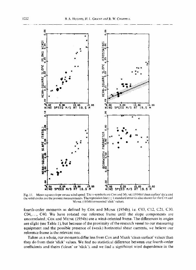
Fig. 11. Mean-square slope versus wind speed. Thex-symbols areCoxand MuNK(1954b)'cteansurface'dataand the solid circles are the present measurements. The regression line ( + I standard error) is also shown for the C( ~x and

MUNK (1954b) crosswind Mick' values.

four th -o rder momen t s as defined by C o x and MUNK (1954b), i.e. C03, C12, C21, C30, C 0 4 , . . . , C40. We have ro ta t ed our reference frame until the s lope c ompone n t s are uncor re la ted ; Cox and MUNK (1954b) use a wind-or ien ted frame. The differences in angles are slight (see Table 1), but because of the p rox imi ty of the research vessel to our measur ing equ ipmen t and the poss ible presence of (weak) hor izon ta l shear currents, we believe our reference frame is the re levant one.

Taken as a whole, our momen t s differ less from Cox and M u n k 'clean surface' values than they do f rom their 's l ick' values. We find no stat is t ical difference between our four th -o rder coefficients and theirs ('clean" or 'slick'), and we find a significant wind dependence in the

A fast response surfitce-wave slope meter and measured wind-wave moments 1223

third-order coefficient C03, as they do for their "clean' surface. We also find a regression slope value for C03 versus wind speed that is statistically the same as theirs, although our intercept value is significantly different (see Table 2). We find no significant wind-speed dependence in C21 (they do for the 'clean' surface), and we find that C12 and C30 are not significantly different from zero (in agreement with their assumption). The second-order coefficients (variances) are shown in Fig. I 1 along with the Cox and Munk 'clean' surhtce values and a single indication of their 'slick" values. We also show the beamwidth parameter a~/a 2. The regression slopes of our variances are not statistically different from their values, but our

2 (with >99~o confidence). In both cases our intercepts are intercepts for a2 and or, 2 + au are nearer to zero than theirs. We do not find any obvious trend in a~/cr z with wind speed.

It should be noted that in all but two of the illustrated jpdf wtlues in Fig. 10 there is a straight-sided part of the lowest depicted contour level. This is evidence that a small percentage of each of these surface wave fields had slopes larger than the (linear) range of the wave slope meter. In calculating high-order statistical moments these large missing points can, of course, be all-important; however, we do not believe their absence has seriously affected the moments presented. It is evident from the probability density functions of Fig. 10 (and the data of Table 2) that excessively large slopes occur with probabilities less than 0.01 of the peak probability. A simple calculation for a Gaussian distribution truncated at

o / " this low level suggests that errors in the fourth-order moments would reach only 15/o, mstead of the recorded scatter of greater than 37~o ('Fable 2).

Frequency spectra have been computed for these data sets (and others), but because the instruments were on a platform moving at about 0.5 m s- ~ there are large Doppler shifts that severely reduce the usefulness of the results. We have succeeded in transforming some of these frequency spectra into wavenumber spectra by using linear dispersion theory and other assumptions. The inversion process, however, is lengthy and complicated and results and methods will not be reported here. [A full account is given by HUGHFS (to be published).]

Acknowledqements It is with great pleasure that we record our thanks to those who contributed to this undertaking, particularly Dr. R. W. STEWART (Institute of Ocean Sciences, Patricia Bay, B.C. ), who provided us with the initial concept for the wave slope meter many years ago, and Dr. E. HARVEY RWHARDSON (Dominion Astrophysical Observatory, Saanich, B.C.t, for designing the large lens. JOHN D. SMITH, A. MOILLIEI, R. S. ANDERSON, and M. C. RASMUSSEN also contributed substantially to one or more of the many phases of the work reported here.

R E F E R E N C E S

Cox C. S. and W. H. MUNK (1954a) Statistics of the sea surface derived from sun glitter. Jourmtl ~?['Marine Reseurch, 13, 198-227.

Cox C. S. and W. H. MUNK (1954b) Measurement of the roughness of the sea surface from photographs of the sun's glitter. Journal ~[the Optical Society ~?f America, 44, 838 -850.

HW;HES B. A. (to be published) The effect of internal waves on surface wind waves. Part II: Theoretical analysis. Journal of Geophysical Research.

HUt;HES B. A. and H. L. GRANT (to be published) The effect of internal waves on surface wind waves. Part 1: Experimental measurements. Journal o['Geophysical Research.

S( OTr J. C. (1974) An optical probe for measuring water wave slopes. Journal (?fPhysics E: Scientific Instruments, 7, 747-749.

STILWELL D., JR. (1969) Directional energy spectra of the sea from photographs. Jaurnul of Geaphysical Research, 74, 1974-1986.

STURM G. V. and F. Y. SORRELL (1973) Optical wave measurement technique and experimental comparison with conventional wave height probes. Applied Optics, 12, 1928-1933.

SUGIMORI Y. (1975) A study of the application of the holographic method to the determination of the directional spectrum of ocean waves. Deep-Sea Research, 22, 339 350.

TOBER G., R. C. ANDERSON and O. H. SHEMDIN (1973) Laser instrument for detecting water ripple slopes. Applied Optics, 12, 788-794.

W u J. (1969) Wind stress and surface roughness at air--sea interface. Journal (?]Geophysical Research. 74, 444--455.

Documents

A fast response surface-wave slope meter and measured wind-wave moments