A fast method for discovering critical edge sequences in e-commerce catalogs

European Journal of Operational Research 181 (2007) 855–871

www.elsevier.com/locate/ejor

Computing, Artificial Intelligence and Information Management

A fast method for discovering critical edge sequencesin e-commerce catalogs q

Kaushik Dutta a,*, Debra VanderMeer a, Anindya Datta b,c,Pinar Keskinocak d,1, Krithi Ramamritham e

a Department of Decision Sciences and Information Systems, Florida International University, Miami, Florida 33199, United Statesb Walking Stick Solutions, 75 Fifth Street NW, Suite 218, Atlanta, Georgia 30308, United States

c School of Information Systems, Singapore Management University, 80 Stamford Rd, Singapore 178902d School of Industrial and Systems Engineering, Georgia Institute of Technology, Atlanta, Georgia 30332, United States

e Department of Computer Science and Engineering, Indian Institute of Technology Bombay, Powai, Mumbai 400076, India

Received 23 July 2005; accepted 30 June 2006Available online 25 October 2006

Abstract

Web sites allow the collection of vast amounts of navigational data – clickstreams of user traversals through the site.These massive data stores offer the tantalizing possibility of uncovering interesting patterns within the dataset. For e-busi-nesses, always looking for an edge in the hyper-competitive online marketplace, the discovery of critical edge sequences

(CESs), which denote frequently traversed sequences in the catalog, is of significant interest. CESs can be used to improvesite performance and site management, increase the effectiveness of advertising on the site, and gather additional knowl-edge of customer behavior patterns on the site.

Using web mining strategies to find CESs turns out to be expensive in both space and time. In this paper, we propose anapproximate algorithm to compute the most popular traversal sequences between node pairs in a catalog, which are thenused to discover CESs. Our method is both fast and space efficient, providing a vast reduction in both the run time andstorage requirements, with minimum impact on accuracy.� 2006 Elsevier B.V. All rights reserved.

Keywords: Data mining; e-Commerce; Graph theory; Applied probability

1. Introduction

Navigational data – clickstreams of user travers-als through web sites – can be used to identify inter-

0377-2217/$ - see front matter � 2006 Elsevier B.V. All rights reserved

doi:10.1016/j.ejor.2006.06.055

q An early version of this work appeared in the ACMConference on Electronic Commerce, 2001.

* Corresponding author. Tel.: +1 305 348 3302.E-mail address: [email protected] (K. Dutta).

1 Pinar Keskinocak is supported by NSF Career Award DMI-0093844.

esting customer behavior. Consider Books.com, afictional online bookseller. Books.com tracks visi-tors as they navigate through the site, and subse-quently analyzes the aggregated data. Assume thatthe analysis reveals the following: (a) if a visitor,in a session, navigates through orchid gardening(OG) and military history (MH), he tends to eventu-ally make a purchase of a music history book; and(b) the shorter the time a user takes to traverse thesite between OG and MH, the higher the likelihood

.

mailto:[email protected]

856 K. Dutta et al. / European Journal of Operational Research 181 (2007) 855–871

of an eventual purchase. Suppose Books.com couldappropriately recognize the popular traversalsequences between OG and MH, and that the anal-ysis of these paths reveals that the most popularsequences are time-consuming to traverse (e.g., ifserver-side delays or large numbers of images leadto large download times, or if the number of clicksrequired is large). This would indicate possible areasof improvement on the site.

Finding popular sequences can be useful in sev-eral other scenarios, for example in predicting tra-versal behavior for caching, or in providingpreferential resource allocation for heavily-tra-versed sequences on the site. For example, if thepath from OG to MH is traversed often, uponnoticing that a user has traversed the OG node,we can prefetch and cache business rules related toMH recommendation content. Then, once the userreaches MH, the relevant recommendations areavailable from cache, removing the need to querythe recommendation engine and reducing the timerequired to serve pages to the user.

Analysis of these sequences can also reveal valu-able patterns that can aid marketing on the site, e.g.,for delivering advertisements, e-coupons, or runningpromotional campaigns [7]. Consider the problemfaced by a marketing manager at an online toy storein developing an adaptive promotional campaignduring the holiday season. During this period, thesite’s sales are greatly impacted by fads and trends– toys become popular virtually overnight [30]. Ifhe can place his targeted advertising and promo-tional material appropriately on the site while thetrend is still growing, he can greatly enhance salesfor a trendy toy. If, however, he must wait severaldays to identify popular traversal sequences, hemay well miss the peak of the trend, leaving signif-icant revenue opportunities on the table.

To motivate the specific problem addressed inthis paper, we return to the example of Books.com.Suppose that an analysis of the popular traversalsequences between OG and MH reveals two distinctsequences:

1. OG! Home Improvement! Anthropology!Medicine!Mythology! Buddhist Literature!MH

2. OG! Computer Science! Anthropology !Medicine!Mythology!Woodworking!MH

It is interesting to note that the most popular tra-versal sequences between OG and MH share a com-

mon subsequence, i.e., anthropology! medicine!mythology, indicating that users frequently traversethis subsequence when navigating from OG toMH (regardless of which exact traversal sequencethey may have followed). We call such edgesequences critical edge sequences (CESs). The focusof this paper is the fast identification of critical tra-

versal patterns at a web site. Our work with a majorclicks-and-mortar, where the extremely rapid dis-covery of such CESs is important, motivated thisresearch. Web-sites need to unearth and react toinformation about CESs rapidly, in matters of min-utes and hours as opposed to days or weeks.

The size of traversal data on web sites is non-triv-ial. Large, high-traffic web sites can generate dailysession logs in the terabyte range. While severalexisting approaches (particularly sequence miningtechniques) can be adapted to find CESs, these algo-rithms require at least one full scan of the log data,resulting in running times on the order of multipledays or weeks, even for computationally efficient(i.e., log-linear or linear) algorithms running onenterprise class servers.

Therefore, we propose efficient and approximate

methods for CES discovery. Our approach to deal-ing with extremely large input datasets is to gathertraversal data in aggregated form (rather than usingweb/application server logs), i.e., we use approxi-mate data and design approximate algorithms forCES discovery, which leads to approximate results.Since the output is approximate, the quality of thesolutions is a concern. To mitigate this concern,we demonstrate that the approximation techniquewe propose allows us to accurately discover mostCESs. Moreover, we provide guidelines for maxi-mizing expected accuracy given a set of inputparameters.

In summary, the contribution of this paper is thepostulation of practical, applicable solutions to theproblem of fast CES discovery. Our case studyresults show accuracy (i.e., number of CESs cor-rectly found as compared to results generated onfull traversal datasets) on the order of 90% obtainedin 15 minute; the corresponding results using fulldata required 18 hour to obtain.

The remainder of this paper is organized as fol-lows. Section 2 describes our model and definesthe CES discovery problem. Section 3 describesour approach to CES discovery and contributions.Section 4 discusses related work. Section 5 presentsour data approximation method, including adescription of how the input is prepared, while Sec-

K. Dutta et al. / European Journal of Operational Research 181 (2007) 855–871 857

tion 6 describes our approximate traversalsequence-finding methods. Section 7 describes CESdiscovery methods, based on the traversal sequencesfound using the methods described in Section 6. Sec-tion 8 presents a case study, demonstrating thereduction in running time and storage requirementsas compared to the full-data case. Section 9 presentsour experimental results, showing the accuracy ofour methods. Section 10 concludes the paper.

2. e-Commerce site model and problem description

We model a site as a graph G = (V,E) similar to[17,13], where each node v 2 V is assigned a uniquenode-id and represents a particular concept in the e-commerce site, e.g., a product or a category of prod-ucts in a hierarchically organized site, and each edgee = (u,v) 2 E represents the links on the site, i.e., thepossible navigation from node u to node v on thesite (where the graph may be cyclic or acyclic). Inthis model, a customer’s traversal through the sitecan be described as a clickstream, i.e., a sequenceof nodes the user visited, and the order in whichhe visited them.

Following [13], our model separates the abstractsite content representation, which corresponds tothe set of nodes and node-ids described above, from

Table 1Summary of notation

Symbol Description

G = (V,E) graph with V vertices and E edgesNi node in the site graph, identified by node-idZ set of possible unique traversal sequences bs 2S subsequence in the set of unique subsequenr 2 R value in the set of traversal frequency valueT threshold frequency, greater than which anf maximum fanout in a site graphl maximum traversal length of a user sessiond depth of previous traversal consideredPV set of vector of probability values associatec cardinality of PV

hNx,Ny,Nzi a traversable edge sequence in G

PðhNi;NjiÞ an element of PV, associated with a particPdðhNi;NjiÞ a vector of traversal probabilities, where jPPðhNi;NjijhNp;Nq;NiiÞ probability that a user will traverse the edg

hNp,Nq,Niik number of MPESs to be foundC count of nodes in a potential CES in N-graqd(hNi,Nji) single value representing the path hNi [ Nj

M the set of k MPESs returnedf the complete set of subsequences in M

m the number of subsequences in M

� the fraction of CESs found in errord the fraction of CESs missed

the concrete page delivered to a user. Essentially, weassume that a user requests content associated witha particular node-id, but may receive additionalcontent associated with multiple other nodes in thesite graph in the delivered page, allowing limitlesscombinations of site content to be generated. Forexample, a user who requests information on thebook ‘‘Gone With The Wind’’ may also receive linksto other historical fiction titles based on resultsretrieved from a recommendation engine. This typeof model reflects the current practice in Web contentdelivery, namely dynamic page generation, wherethe pages served to a user are generated on the fly,based on the site’s business logic and the user’s stateat run-time.

The notation used throughout the remainder ofthe paper is summarized in Table 1.

Having discussed our model, we now formallydescribe the problem of discovering CESs.

Consider a Web site graph G = (V,E). Supposewe are given a start node Na 2 V, and an end nodeNb 2 V, such that Nb is reachable from Na. Let Zdenote the set of (possibly partially overlapping)unique traversal sequences (paths) in G from Na toNb. Let J denote the binary relation ðS;RÞ, whereS denotes the set of unique subsequences comput-able from any element in Z, R is a set of frequency

i

etween a start node and an end nodeces computable from Z

s for edge subsequences in S

edge sequence is deemed critical

d with traversed edges in G

ular traversed edge hNi,Nji in G

dðhNi;NjiÞj is the number of d-length paths leading to Ni

e hNi,Nji, given that he arrives at Ni by traversing the sequence

m analysisi

Table 2Subsequences and traversal frequencies in example CES analysis

Traversalfrequency f

Subsequence s

20 hOG,HI,ANi, hHI,AN,MEi, hME,MY,WOi,hMY,WO,MHi

40 hOG,CS,ANi, hCS,AN,MEi, hME,MY,BLi,hMY,BL,MHi

60 hAN,ME,MYi


values, and (si, ri) (si 2 S and ri 2F) denotes thatthe sequence si was traversed ri times. We refer tosi as an ‘‘edge sequence’’ in G and ri as the ‘‘fre-quency of traversal’’ of edge sequence si. A CESof Na and Nb in G is any edge sequence si 2S suchthat ri P T, where T is a configurable, pre-deter-mined threshold frequency.

The goal of our approach is to identify the longest

possible CESs that satisfy the frequency criteria T.By definition, each subsequence of a CES is itselfa CES. In our result set, however, we do not needto enumerate each subsequence-based CES. Forexample, if the sequences hN1,N2,N3i andhN3,N4,N5i both meet the frequency criteria T,our algorithm would return the sequencehN1,N2,N3,N4,N5i, rather than the two shortersequences.

Example: In Fig. 1, the sequences marked Ma,Mb, and Mc represent frequently traversed pathsbetween OG and MH. In this example, each pathhas been traversed 20 times. We consider subse-quences – potential CESs – of three nodes each tokeep the discussion brief, yet still provide insightinto the CES definition.

From Fig. 1, we can find Z:

Z ¼ fhOG;HI;AN;ME;MY;BL;MHi;hOG;CS;AN;ME;MY;BL;MHi;hOG;CS;AN;ME;MY;WO;MHig¼ fMa;Mb;Mcg

In S, there are nine edge sequences consisting ofthree nodes as shown in Table 2. For T P 60, onlythe sequence hAN,ME,MYi qualifies as a CES. ForT P 40, sequences hOG,CS, ANi, hCS,AN,MEi,hME,MY,BLi, and hMY, BL,MHi would qualifyas well.

The CES discovery problem can be formally sta-ted: given a web site graph G and a mechanism for

observing navigation over G, design algorithms to

Fig. 1. Example traversal graph from the Books.com site graph.

rapidly, efficiently, and accurately discover CESs,

given specific start and end nodes. Our approachcan easily be extended to find all CESs in the e-com-merce catalog irrespective of specific start and endpoints.

3. An overview of our approach to finding

critical edge sequences

To discover CESs between the node pair (Na,Nb)we follow a three-step approach: (1) observe user

traversals between Na and Nb and accumulate tra-

versal data; (2) based on the data collected in step

(1), discover the most popular edge (traversal)

sequences (MPESs) between Na and Nb; and (3)based on the MPESs discovered in step (2), identify

CESs.

3.1. Accumulating traversal data

Due to the prohibitively large data volumes inweb logs, analyzing the full log data and applyingexisting web mining algorithms to exactly identifythe MPESs on a site is impractical. Consider theclicks-and-mortar site where we tested our methods.On average, this site experiences 10 million uniqueuser sessions in a day. Each user requests, on aver-age, 10 pages on the site. A log entry on this siteconsists of some 300 bytes of data, and each userclick, on average, generates 15 log entries (sinceeach embedded object requested from the site, e.g.,image files, is logged separately). In this case, thesize of the log file generated per day is10,000,000 · 10 · 300 · 15 bytes or 0.45 TB. Overthe course of a single year, the data volume growsto almost 164 TB. There exist techniques, such asthose described in [14], by which it is possible tostore only the meaningful clickstreams (by deletingthe web log records of embedded objects and by rep-resenting each page by a unique id corresponding tothe e-catalog). Typically, such filtering will reducethe daily log file size to 5% of the original size


[14], resulting in a daily log size of 22.5 GB andyearly log size of at least 8 TB for this site. Manysites (e.g., Yahoo! [31], which serves more than600 million pages per day), produce log sizes ordersof magnitude larger than those of our clicks-and-mortar site.

These data sets are still too large for rapid anal-ysis. Therefore, we aggregate traversal data as wegather it. Our proposed data-gathering techniquedoes not maintain a record of each traversal ofinterest, but rather maintains counts of such travers-als aggregated across all users, which significantlyreduces the overall data size over filtering tech-niques. For example, the aggregated data for theoptimal setting for our algorithm produces areduced size of 45.4 MB as compared to the corre-sponding filtered log size of 4 GB for 3 hour tra-versal data. Due to aggregation, this percentagedrops further over time. In the case of large sites likeYahoo, the aggregated data size for a year wouldlikely be in the low-GB range. For the e-catalog sitethat motivated this paper, the aggregated data sizefor a year’s worth of data would be a few hundredMB.

To aggregate the traversal data, we store multiple

counts of traversals through each node, based on a

limited number of nodes traversed to reach it (see Sec-tion 5 for details). This results in approximated tra-versal data, with significant reductions in storagerequirements over the full-storage case (see the casestudy in Section 8).

3.2. Finding the most popular edge sequences

Based on the data accumulated using our data-gathering strategy, we next seek to identify theMPESs – the most frequently traversed sequencesbetween a pair of nodes. (With reference to ourexample in Section 5, the traversal paths Ma, Mb,and Mc represent MPESs between the nodes OGand MH.) We propose algorithms for this purpose(see Section 6 for details), inspired by known pathtraversal algorithms, designed to provide accurate

solutions quickly. The output is a set of k MPESs,where k is a configurable number of most popularedge sequences to be found.

3.3. Finding critical edge sequences from MPESs

Based on the MPESs found, we need to find theactual CESs, which are the subsequences of MPESs(and, potentially, actual MPESs) that meet the fre-

quency threshold criteria T. To find the CESs, weneed to consider the overlapping subsequencesacross the set of MPESs (see Section 7 for details).Though we specifically concentrate on finding CESsbetween two nodes, our approach can easily beextended to find CESs between multiple nodes.

4. Related work

The problem of finding the MPESs, the most dif-ficult part of the CES discovery process, maps nicelyto sequence mining discovery [5,11,8,22,24] which isa standard approach for finding sequential patternsin a dataset. Web usage mining (e.g., [8,22,26,18,23])is a sub-area within the area of sequence miningparticularly applicable to the MPES-discoveryproblem. Much work on algorithms for web usagemining (e.g., [15,21,14,27,26,32]) is based on datamining [1,2,4,19] and sequential mining in particular[3,29]. Virtually all approaches in area take filteredweb logs (i.e., full traversal data) as input, andoutput exact sequential patterns matching some cri-teria. For example, [18] finds all repeating subse-quences meeting a minimum frequency threshold,while [23] suggests a document prefetching schemebased on a user’s next predicted action on a site.

There exists other research that applies sequencemining techniques in mining web logs, some exploit-ing multi-threaded and multi-processor systems. Allthese approaches require at least one full scan of thelog data, resulting in long run times for large logdatasets. For example, SPADE [21] requires threefull scans of the log data. Both webSPADE [14]and ASIPATH [15] are parallel-algorithm varia-tions of SPADE developed for web logs, and requireone full scan of the log data and multi-processorservers. As we demonstrate in Section 8, comparedto these algorithms, our approach gives near real-time performance on a standard single processorserver.

In [20], Kum et al., propose an approximatemethod for sequence mining. However, theirapproach considers a different, ‘‘looser’’, definitionof a sequence than we do. Specifically, if there existsa sequence hN1,N2,N3,N4,N5i, [20] will considerhN1,N3,N4i and hN1,N2,N4i as valid subsequences.By this definition of a subsequence, most of the sub-sequences used in analysis will likely not haveoccurred consecutively in the original sequences.In contrast, mining critical edge sequences requiressuch consecutiveness, otherwise the results mayyield non-existent paths on the web. For this reason,


we cannot directly apply their work. The difficulty of

applying existing methods to our problem was the pri-

mary motivator in designing an approximate solution

for MPES discovery.

5. Gathering approximate data

For efficient CES analysis, it is impractical tostore and manipulate large volumes of data. There-fore we develop a data approximation strategywhich results in a significantly smaller input dataset.

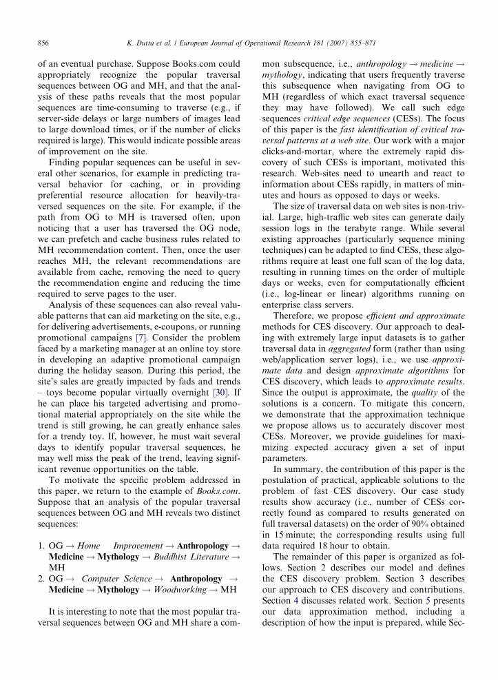
One simple approach to approximate data stor-age is to store only the edges in the graph (i.e., pathswith two nodes, or 2-length paths). However, thespecific path a customer follows before coming toa particular node usually impacts which path he willfollow leaving the node. Storing only 2-length pathsdoes not allow us to capture such information. Anintermediate solution is to store information aboutd-length paths (i.e., paths with d edges and d + 1nodes) that lead to a particular node, and their fre-quencies. For example, in Fig. 2 we have a total of 7paths that pass through node N2 and 3 3-lengthpaths arriving at node N2. We have the followingcount on the traversals of these 3-length paths: 3customers traversed hN3,N1,N2i, 3 customers tra-versed hN4,N1,N2i, and 1 customer traversedhN5,N1,N2i.

We want to store the probability that a customerwill traverse a particular edge after arriving at nodeN2, given that the customer came to N2 following aparticular 3-length path. For example, the probabil-ity that a customer will traverse hN2,N11i given that

6

7

10

49

8

5

1 2 11

312

13

UaUbUcUdUe

UgUf

Fig. 2. Example traversal graph.

he arrived at N2 through hN3,N1,N2i is PðhN 2;N 11ijhN 3;N 1;N 2iÞ ¼ 0:67, since two out of three pathsthat arrive at N2 through hN3,N1,N2i continue toN11. Similarly, the probability that a customer willtraverse hN2,N11i given that he arrived at N2

through hN4,N1,N2i is PðhN 2;N 11ijhN 4;N 1;N 2iÞ ¼0:67. Finally, the probability that a customer willtraverse hN2,N11i given that he arrived at N2

through hN5,N1,N2i is 0.More formally, our approximate input data, in

this context, may be thought of as a binary relationðE;PVÞ, with tuples of the form (ei,pvi) where ei is atraversed edge in G, i.e., ei 2 E and pvi is a probabil-ity vector hp1,p2, . . .,pci, pi 2 PV. The cardinalityof PV, i.e., the value of c, is the number of possibled-length traversal paths in G leading into ei, and pj

denotes the probability that a visitor in G will tra-verse the edge ei, given that he has arrived at thestart node of ei by traversing the jth d-length pathincident on this start node.

Gathering and aggregating input data consists oftwo distinct steps: (a) session information is accu-mulated while visitors are traversing the site(described in detail in the Appendix); and (b) prob-ability vectors are computed in batch mode from thecollected session information obtained in step (a).New clickstreams are periodically integrated viabatch mode processing into the aggregated traversaldataset, i.e., the pre-processing step takes place in

small increments over time; the algorithm never con-

siders the full traversal data as input.In general, for some d > 1, say, d = 3, we con-

sider dependence up to 3 nodes (2 edges), i.e., wehave information about sequences of length 3, andassume that the probability of traversing an edgeis dependent on only the three most recently tra-versed nodes; all previous traversals are assumedto be independent. When d = l, where l is the max-imum user session length, we have complete infor-mation about the sessions. Another way oflooking at depth d is to model a user’s future tra-versal behavior as a Markov chain, where d = 1 cor-responds to a first-order Markov model, and d = i

corresponds to an (i)th order Markov model.Clearly, the cost and accuracy of the result is a

function of d: larger d values correspond to moredetailed information about sessions, larger storagerequirements and more accurate results. We areinterested in exploring the cost/accuracy tradeoffof varying d (the only tunable parameter in ourapproach). We address two questions: (a) to what

degree does this independence assumption affect accu-


racy? (b) how does accuracy scale, i.e., does increas-

ing depth provide marginal returns? We explore thesequestions in detail in Section 9.2.2, in the context ofour experimental results.

6. Algorithmic approximation

We present the configurable-depth algorithm

(CDA) for finding MPESs, given varying degreesof information (varying values of d) about user tra-versals and hence varying dependence assumptionsregarding prior traversal. CDA is a variant of Dijk-stra’s single-source shortest-path (SSSP) algorithm,2

Shier’s single-source k shortest-paths algorithm [25]or Eppstein’s k shortest-paths algorithm [16]. Thesimilarities between the problems underlying bothSSSP and CDA are clear: both consider pathsthrough a graph and seek to find the ‘‘best’’ paths– SSSP considers ‘‘best’’ to be the least sum ofedge-weights, while ‘‘best’’ for CDA is the path withthe highest probability of traversal.

The differences between CDA and Shier’s k-SSSPlie in the values and functions used in finding the‘‘best’’ paths. Specifically, CDA varies from Shier’sk-SSSP in the following ways: (a) the meaning ofthe edge weights; (b) the fitness function for a path;and (c) the function used to compare paths to oneanother. We discuss each of these differences in turn.

6.1. Edge weight in CDA

Shier’s k-SSSP uses a positive integer value, rep-resenting the length (weight) of the edge, whereasCDA uses the probability of traversal of an edge(see Section 5) as the weight of the edge. Ford = 1, this probability is a scalar value, whereasfor d > 1, we have a vector of probabilities for tra-versing a particular edge, one probability value foreach unique path of length d leading up to thesource node of the edge.

6.2. Path weight function in CDA

In Shier’s k-SSSP, the weight of a path isdescribed as the sum of edge weights of that path,whereas in CDA, the path weight is the product ofthe probabilities of the edge weights in the path.

2 We also considered Floyd’s all-pairs shortest path algorithm,but found that it would compute many more sets of MPESs thanneeded, since most Web sites have only a small set of high-frequency start nodes.

For d = 1, we can use scalar multiplication. Ford > 1, we define a path weight function, CDA-MULT, which handles vectors of probability valuesfor each edge.

We define a path probability PðhN 1;N 2; . . . ;N kiÞfor path hN1,N2, . . ., Nki in terms of the edge prob-abilities PdðhN i;NjiÞ, for edges (Ni,Nj) 2 E as thevector multiplication of probabilities of edges on apath. Specifically, we define the multiplication ofedge probability vectors PdðhN i;N jiÞ ¼ PdðhNi;NqiÞ �PdðhN q;NjiÞ, where Nq is an intermediatenode for path Ni [ Nj, as follows, given that thepath hN 01;N 02; . . . ;N 0ðd�1Þi is on the path hN1,N2, . . .,N(d�1),Ni [ Nqi and N 0ðd�1Þ is the node just beforenode Nq on the path Ni [ Nqi:

if PðhN i;NjijhN 1;N 2; . . . ;N ðd�1Þ;NiiÞ2 PðhNi;NjiÞ

and PðhN i;NqijhN 1;N 2; . . . ;N ðd�1Þ;N iiÞ2 PdðhN i;NqiÞ

and PðhN q;NjijhN 01;N 02; . . . ;N 0ðd�1Þ;NqiÞ2 PdðhN q;NjiÞ

then PðhN i;NjijhN 1;N 2; . . . ;N ðd�1Þ;NiiÞ¼ hPðhN i;NqijhN 1;N 2; . . . ;N ðd�1Þ;NiiÞ�PðhNq;N jijhN 01;N 02; . . . ;N 0ðd�1Þ;N qiÞi

ð1Þ

To clarify these notions, we consider the exampleof finding the probabilities of paths ending athN2,N11i in Fig. 2 with depth d = 3. Before calculat-ing path probabilities, we need to first find the edgeprobabilities for P3ðhN 2;N 11iÞ, P3ðhN 1;N 2iÞ, andP3ðhN 1;N 11iÞ. For example, the edge probabilityvector for P3ðhN 2;N 11iÞ is as follows:

P3ðhN 2;N 11iÞ ¼ hPðhN 2;N 11ijhN 3;N 1;N 2iÞ;

PðhN 2;N 11ijhN 4;N 1;N 2iÞ;

PðhN 2;N 11ijhN 5;N 1;N 2iÞi

The edge probability vectors for P3ðhN 1;N 2iÞ,and P3ðhN 1;N 11iÞ are generated similarly.

Using these edge probabilities and vector multi-plication, we can find path probabilities. For exam-ple, we find the path probability:

PðhN 1;N 11ijhN 7;N 3;N 1iÞ¼ PðhN 1;N 2ijhN 7;N 3;N 1iÞ�PðhN 2;N 11ijhN 3;N 1;N 2iÞ ð2Þ

Path probabilities for PðhN 1;N 11ijhN 6;N 3;N 1iÞ,PðhN 1;N 11ijhN 8;N 4;N 1iÞ, PðhN 1;N 11ijhN 9;N 4;N 1iÞ,

<Nd>

<Nd,Na,Ne>

<Ne><Nc>

<Nc,Na>

<Nc,Na,Ne>

<Nd,Na>

<Na>

<Na,Nb> <Na,Ne>

<Na,Nb,Nc> <Na,Nb,Nd>

<Na,Nb,Nc,Na>

<Na,Nb,Nc,Na,Ne>

<Na,Nb,Nd,Na>

<Na,Nb,Nd,Na,Ne>

<Nb>

<Nb,Nd>

<Nb,Nd,Na,Ne>

<Nb,Nc,Na,Ne>

<Nb,Nd,Na>

<Nb,Nc>

<Nb,Nc,Na>

C=4

C=2

<empty>

C=2

C=1

C=1

C=1 C=1

C=1

C=1

C=1

C=1

C=1

C=1

C=1

C=1

C=1 C=1 C=1

C=1C=1

C=1 C=1

C=2

Fig. 3. Example tree representation for CES data.


and PðhN 1;N 11ijhN 10;N 5;N 1iÞ are computed in asimilar fashion.

6.3. Path comparison function in CDA

In order to find the k most-traversed paths, weneed a means of comparing paths to one another.In CDA, instead of the minimization functionfound in shortest paths algorithms, we use a maxi-mization function. In order to do this, we define afunction for path comparison, CDA-MAX. If wehave two probability vectors P0 and P00, then wecan define the CDA-MAXðP0;P00Þ as follows:

CDA-MAXðP0;P00Þ ¼P0 if

P8p02P0

p0 PP8p002P00

P00

P00 otherwise

8<:

That is, between two paths for Ni [ Nj with theircorresponding probability vectors P0 and P00 wechoose the path which has the highest sum of prob-ability values in the probability vector.

In order to use CDA-MAX, we must be able torepresent a path as a single value, rather than as avector of values. To achieve this, we defineqd(hNi,Nji) as the sum over the d-depth probabilitiesin the path Ni [ Nj: qdðhNi;N jiÞ ¼

P8p2PðhNi ;NjiÞp.

3 We note here that other sub-string matching algorithms, e.g.,those described in [10], can also be applied.

7. Finding critical edge sequences

We next describe how to actually derive CESsfrom a set of k MPESs (the output of the CDA algo-rithm described in Section 6). Given a set of k

unique paths with at most l nodes, our goal is to findall matching edge sequences across those k paths,where the length of a matching sequence can range

from 1 to l � 1 (a matching sequence of length l

would indicate a non-unique set of k paths).Fortunately, existing work in pattern matching

can be applied to this problem. Specifically, wemake use of work in N-gram analysis [9,6] fromthe areas of natural language processing (NLP)and information retrieval (IR).3 N-gram analysis isused in NLP to find the Markovian probability ofthe nth phoneme (i.e., sound) following a sequenceof n � 1 phonemes – one application of this is inspeech recognition. IR uses a similar approach withwords instead of characters to support text-retrievalapplications.

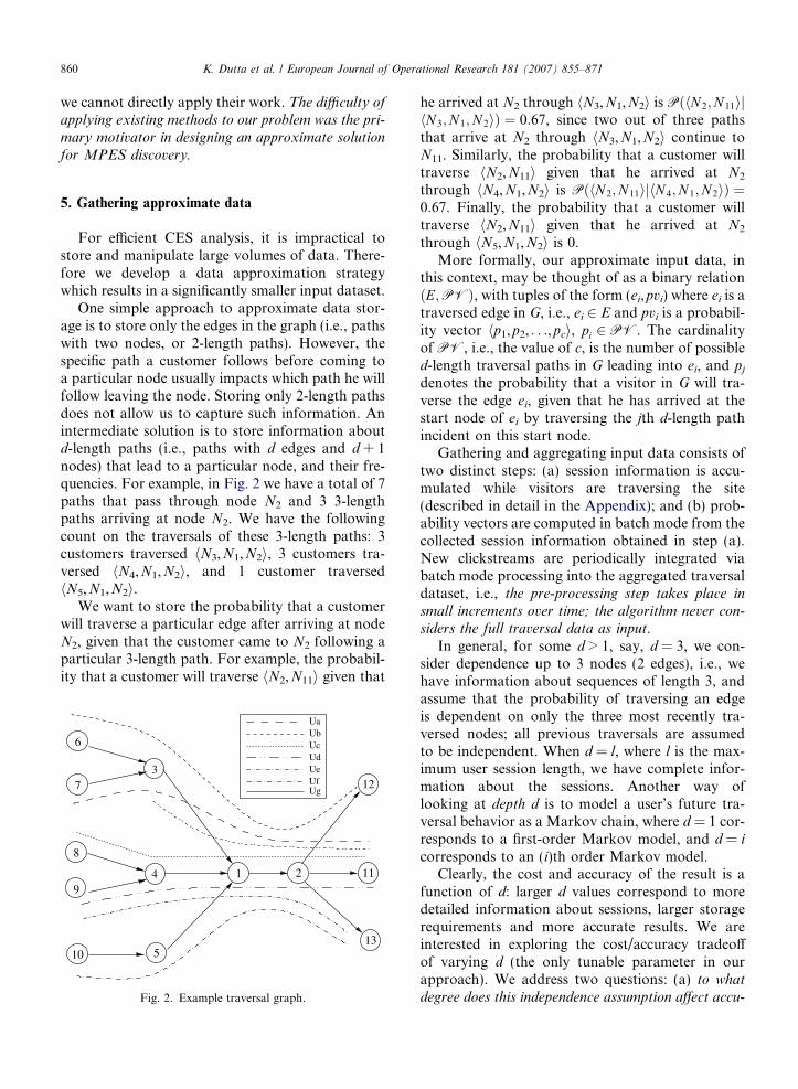
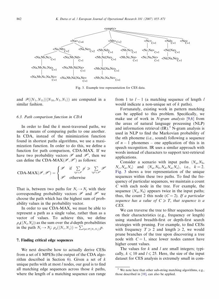
Consider a scenario with input paths hNa,Nb,Nc,Na,Nei and hNa,Nb,Nd,Na,Nei, i.e., k = 2.Fig. 3 shows a tree representation of the uniquesequences within these two paths. To find the fre-quency of particular sequences, we maintain a countC with each node in the tree. For example, thesequence hNa,Nbi appears twice in the input paths;thus, the count 2 this node (C = 2). If a particular

sequence has a value of C P T, that sequence is a

CES.

We can traverse the tree to filter sequences basedon their characteristics (e.g., frequency or length)using standard breadth-first or depth-first searchstrategies with pruning. For example, to find CESswith frequency T P 2 and length P 2, we wouldprune branches of the tree upon discovering a treenode with C = 1, since lower nodes cannot havehigher count values.

The values for k and l are small integers; typi-cally, k 6 10 and l 6 25. Here, the size of the inputdataset for CES analysis is extremely small in com-


parison to the input dataset for finding the k mosttraversed paths. Thus, rather than discussing thetime and space complexity of N-gram analysis indepth, we refer the reader to [9].

8. CDA case study

We present a case study, based on data gatheredfrom traversal logs over a 150,000-product e-com-merce site, demonstrating the space and runningtime savings of CDA over full-data analysis.

For each of four time periods, we collected a full-

traversal dataset and two approximate data sets,resulting in 12 sets of data. The full-data set storescomplete traversal sequences, while the other twodata sets store approximate data for d = 3 andd = 4. We analyzed each data set for k = 3 using aDell PowerEdge server with a single 3.0 GHzCPU, 2 GB RAM, and 120 GB of hard disk space.

To perform the full-data analysis, we chose theWeb Utilization Miner (WUM) tool [27] because itincorporates a query processor, allowing the specifi-cation of arbitrary patterns of interest (e.g., arbi-trary start and end points) in the query languageMINT [28], and is known to implement efficientalgorithms and provide fast running times [27]. InSection 9, we use WUM as a benchmark, comparingits performance to that of our approach in terms ofaccuracy.

To use WUM to find the MPESs between twospecified nodes, Na and Nb, on a web site, we pro-vided web log data and the following MINT queryto the WUM tool:

• select t from node as a b, template a * b as t where

a.url = ‘‘Na’’ and b.url = ‘‘Nb’’ and (b.support/

a.support) > 0.1

Table 3Case study comparing space and running times for CDA and full-data

Time period Data type

50 minute Full50 minute Approximate, d = 350 minute Approximate, d = 41.5 hour Full1.5 hour Approximate, d = 31.5 hour Approximate, d = 42.5 hour Full2.5 hour Approximate, d = 32.5 hour Approximate, d = 43 hour Full3 hour Approximate, d = 33 hour Approximate, d = 4

In this query, a * b represents a regular expres-sion pattern to be matched, where a is the start nodeand b the end node, while the * matches anysequence of zero or more nodes between the startand end points. The restriction b.support/a.sup-

port > 0.1 restricts the number of MPESs from Na

to Nb, retaining only those sequences where at least10% of the users who arrived at Na traversed to Nb.Once we have the results from the MINT query, wecan easily sort on the support restriction to find thek MPESs.

Table 3 shows the time period each dataset repre-sents, as well as the storage and running times.Clearly, the approximated datasets result in signifi-cantly less storage and lower running times thanthe full-data set (at least two, in some cases threeorders of magnitude improvement). We find thatincrementing d from 3 to 4 has adds roughly a 3·increase in running time and storage requirements.We describe the variation in accuracy between thesetwo cases in Section 9.2.

9. Accuracy evaluation

To evaluate the accuracy of our algorithms, wecompare the quality of the output CDA to that ofWUM (where WUM produces fully accurate resultsbecause it considers the full data as input). Wewould like to determine to what extent varying theindependence assumption (as encoded by d) affectsaccuracy. Next, we describe our accuracy metricsand the results of our experiments.

9.1. Accuracy metrics

To measure the performance of our algorithms,we first describe how one can compare the two sets

analysis

Space required Running time

1 GB 2 hour10.1 MB 4.2 minute34 MB 12 minute2 GB 6 hour17.3 MB 5.3 minute54.2 MB 18.2 minute3 GB 18 hour31.9 MB 9.2 minute99.3 MB 33 minute4 GB 38 hour45.4 MB 15 minute112.5 MB 45 minute

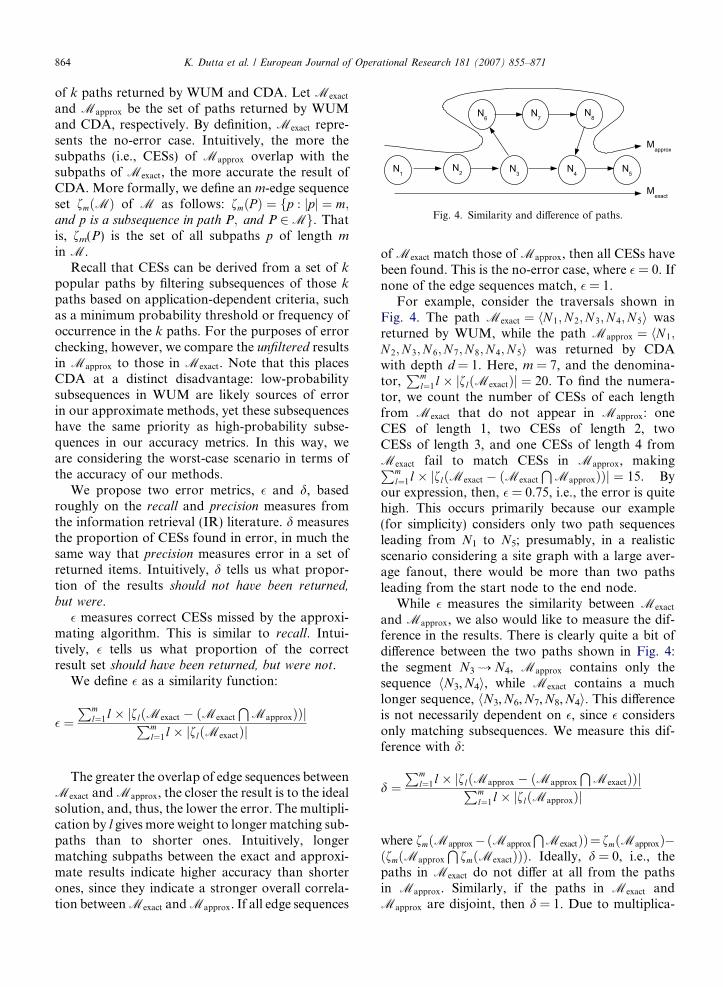
Fig. 4. Similarity and difference of paths.


of k paths returned by WUM and CDA. Let Mexact

and Mapprox be the set of paths returned by WUMand CDA, respectively. By definition, Mexact repre-sents the no-error case. Intuitively, the more thesubpaths (i.e., CESs) of Mapprox overlap with thesubpaths of Mexact, the more accurate the result ofCDA. More formally, we define an m-edge sequenceset fmðMÞ of M as follows: fmðP Þ ¼ fp : jpj ¼ m;and p is a subsequence in path P; and P 2Mg. Thatis, fm(P) is the set of all subpaths p of length m

in M.Recall that CESs can be derived from a set of k

popular paths by filtering subsequences of those k

paths based on application-dependent criteria, suchas a minimum probability threshold or frequency ofoccurrence in the k paths. For the purposes of errorchecking, however, we compare the unfiltered resultsin Mapprox to those in Mexact. Note that this placesCDA at a distinct disadvantage: low-probabilitysubsequences in WUM are likely sources of errorin our approximate methods, yet these subsequenceshave the same priority as high-probability subse-quences in our accuracy metrics. In this way, weare considering the worst-case scenario in terms ofthe accuracy of our methods.

We propose two error metrics, � and d, basedroughly on the recall and precision measures fromthe information retrieval (IR) literature. d measuresthe proportion of CESs found in error, in much thesame way that precision measures error in a set ofreturned items. Intuitively, d tells us what propor-tion of the results should not have been returned,

but were.� measures correct CESs missed by the approxi-

mating algorithm. This is similar to recall. Intui-tively, � tells us what proportion of the correctresult set should have been returned, but were not.

We define � as a similarity function:

� ¼Pm

l¼1l� jflðMexact � ðMexact

TMapproxÞÞjPm

l¼1l� jflðMexactÞj

The greater the overlap of edge sequences betweenMexact and Mapprox, the closer the result is to the idealsolution, and, thus, the lower the error. The multipli-cation by l gives more weight to longer matching sub-paths than to shorter ones. Intuitively, longermatching subpaths between the exact and approxi-mate results indicate higher accuracy than shorterones, since they indicate a stronger overall correla-tion between Mexact and Mapprox. If all edge sequences

of Mexact match those of Mapprox, then all CESs havebeen found. This is the no-error case, where � = 0. Ifnone of the edge sequences match, � = 1.

For example, consider the traversals shown inFig. 4. The path Mexact ¼ hN 1;N 2;N 3;N 4;N 5i wasreturned by WUM, while the path Mapprox ¼ hN 1;N 2;N 3;N 6;N 7;N 8;N 4;N 5i was returned by CDAwith depth d = 1. Here, m = 7, and the denomina-tor,

Pml¼1l� jflðMexactÞj ¼ 20. To find the numera-

tor, we count the number of CESs of each lengthfrom Mexact that do not appear in Mapprox: oneCES of length 1, two CESs of length 2, twoCESs of length 3, and one CESs of length 4 fromMexact fail to match CESs in Mapprox, makingPm

l¼1l� jflðMexact � ðMexact

TMapproxÞÞj ¼ 15. By

our expression, then, � = 0.75, i.e., the error is quitehigh. This occurs primarily because our example(for simplicity) considers only two path sequencesleading from N1 to N5; presumably, in a realisticscenario considering a site graph with a large aver-age fanout, there would be more than two pathsleading from the start node to the end node.

While � measures the similarity between Mexact

and Mapprox, we also would like to measure the dif-ference in the results. There is clearly quite a bit ofdifference between the two paths shown in Fig. 4:the segment N3 [ N4, Mapprox contains only thesequence hN3,N4i, while Mexact contains a muchlonger sequence, hN3,N6,N7,N8,N4i. This differenceis not necessarily dependent on �, since � considersonly matching subsequences. We measure this dif-ference with d:

d ¼Pm

l¼1l� jflðMapprox � ðMapprox

TMexactÞÞjPm

l¼1l� jflðMapproxÞj

where fmðMapprox�ðMapprox

TMexactÞÞ¼ fmðMapproxÞ�

ðfmðMapprox

TfmðMexactÞÞÞ. Ideally, d = 0, i.e., the

paths in Mexact do not differ at all from the pathsin Mapprox. Similarly, if the paths in Mexact andMapprox are disjoint, then d = 1. Due to multiplica-

0

0.2

0.4

0.6

0.8

1

1 2 3 4 5

Eps

ilon

k

WUMDepth=4Depth=3Depth=2Depth=1

Fig. 5. Accuracy � as d varies over a synthetic dataset.


tion by l, the longer the non-matching subpath, thegreater the error, and the higher the d value.

In the example in Fig. 4, m = 7, andPm

l¼1l�jflðMapprox � ðMexact

TMexactÞÞj ¼ 79, since there

are 4 CESs of length one in Mapprox but notMexact, as well as 5 CESs of length two, 5 CESs oflength three, 4 CESs of length four, 3 CESsof length five, 2 CESs of length six, and 1 CESof length seven. The denominator,

Pml¼1l�

jflðMapproxÞj ¼ 84, since there are 84 possible CESmatches. Thus, d = 0.94 in this example, which isquite high. This occurs for the same reasons as inthe case of � – the small number of paths compared.

9.2. Experimental results

In this section, we report the results of our exper-iments. In particular, we are interested in how wellthe algorithms find the CESs given varying assump-tions of dependence (depth d), as well as the CDAalgorithm’s sensitivity to fanout in the graph andtraversal locality.

9.2.1. Baseline experimental results

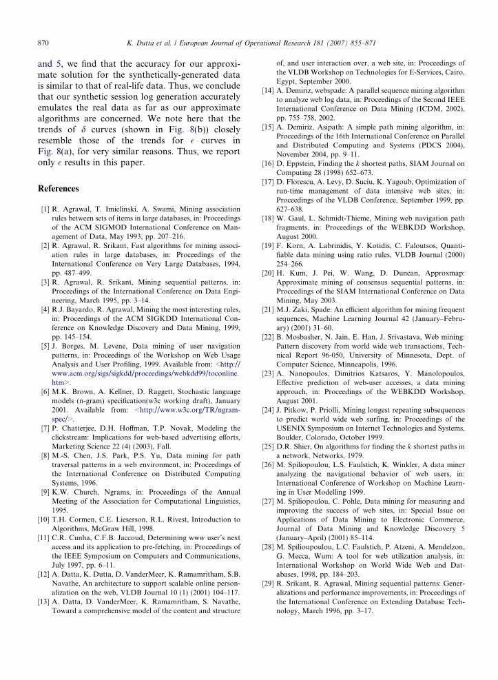
Our baseline experiment considers the effect ofthe depth d on the accuracy of the results. While itis possible to show results for our baseline experi-ments using real data (as described in our case studyin Section 8), we cannot easily modify the character-istics of a live site graph, as is needed for our sensi-tivity experiments. Thus, we generate a syntheticdataset closely resembling our real dataset for thepurposes of our sensitivity experiments. The detailsof how we generated the synthetic dataset are pre-sented in the Appendix.

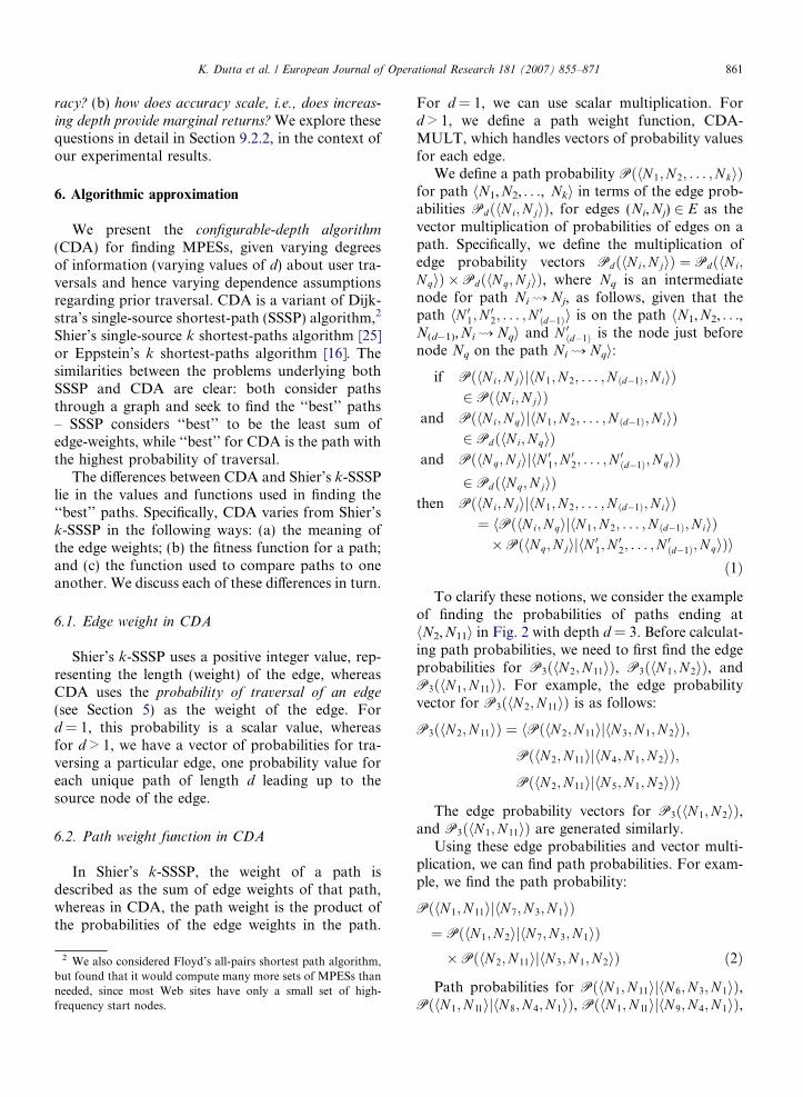
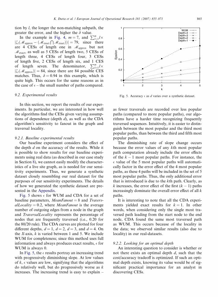
Fig. 5 shows � for WUM and CDA for a set ofbaseline parameters, MeanFanout = 8 and Travers-

alLocality = 0.2, where MeanFanout is the averagenumber of outgoing edges from a node in the graphand TraversalLocality represents the percentage ofnodes that are frequently traversed (i.e., 0.20 forthe 80/20 rule). The CDA curves are plotted for fourdifferent depths, d = 1, d = 2, d = 3, and d = 4. Onthe X-axis, k is varied between 1 and 5. We includeWUM for completeness; since this method uses fullinformation and always produces exact results, � forWUM is always 0.

In Fig. 5, the � results portray an increasing trendwith progressively diminishing slope. At low valuesof k, � values are low, signifying that the algorithmsdo relatively well, but do progressively worse as k

increases. The increasing trend is easy to explain –

as fewer traversals are recorded over less popularpaths (compared to more popular paths), our algo-rithms have a harder time recognizing frequentlytraversed sequences. Intuitively, it is easier to distin-guish between the most popular and the third mostpopular paths, than between the third and fifth mostpopular paths.

The diminishing rate of slope change occursbecause the error values of any kth most popularpath computation already include the error effectsof the k � 1 most popular paths. For instance, the� value of the 5 most popular paths will automati-cally factor in the error effect of the 4 most popularpaths, as these 4 paths will be included in the set of 5most popular paths. Thus, the only additional errorthat is introduced is due to the kth path. Clearly, ask increases, the error effect of the first (k � 1) pathsincreasingly dominate the overall error effect of all k

paths.It is interesting to note that all the CDA experi-

ments yielded exact results for k = 1. In otherwords, when considering only the single most tra-versed path leading from the start node to the endnode, CDA found the same most traversed pathas WUM. This occurs because of the locality inthe data; we observed similar results (also due tolocality) in our real-datasets.

9.2.2. Looking for an optimal depth

An interesting question to consider is whether ornot there exists an optimal depth d, such that thecost/accuracy tradeoff is optimized. If such an opti-mal depth exists, knowing its value would be of sig-nificant practical importance for an analyst indiscovering CESs.

0

0.2

0.4

0.6

0.8

1

1 2 3 4 5 6

Nor

mal

ized

Tim

e/S

tora

ge/E

psilo

n

Depth (d)

Normalized Storage SizeNormalized Time

Normalized Epsilon

Fig. 6. Cost of accuracy.

Table 4Parameters of synthetic data

Parameter Baseline Minimum Maximum

Average Fanout 8 3 15Locality 0.2 0.1 0.3


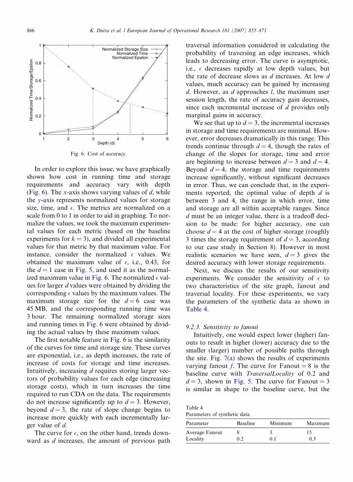
In order to explore this issue, we have graphicallyshown how cost in running time and storagerequirements and accuracy vary with depth(Fig. 6). The x-axis shows varying values of d, whilethe y-axis represents normalized values for storagesize, time, and �. The metrics are normalized on ascale from 0 to 1 in order to aid in graphing. To nor-malize the values, we took the maximum experimen-tal values for each metric (based on the baselineexperiments for k = 3), and divided all experimentalvalues for that metric by that maximum value. Forinstance, consider the normalized � values. Weobtained the maximum value of �, i.e., 0.43, forthe d = 1 case in Fig. 5, and used it as the normal-ized maximum value in Fig. 6. The normalized � val-ues for larger d values were obtained by dividing thecorresponding � values by the maximum values. Themaximum storage size for the d = 6 case was45 MB, and the corresponding running time was3 hour. The remaining normalized storage sizesand running times in Fig. 6 were obtained by divid-ing the actual values by these maximum values.

The first notable feature in Fig. 6 is the similarityof the curves for time and storage size. These curvesare exponential, i.e., as depth increases, the rate ofincrease of costs for storage and time increases.Intuitively, increasing d requires storing larger vec-tors of probability values for each edge (increasingstorage costs), which in turn increases the timerequired to run CDA on the data. The requirementsdo not increase significantly up to d = 3. However,beyond d = 3, the rate of slope change begins toincrease more quickly with each incrementally lar-ger value of d.

The curve for �, on the other hand, trends down-ward as d increases, the amount of previous path

traversal information considered in calculating theprobability of traversing an edge increases, whichleads to decreasing error. The curve is asymptotic,i.e., � decreases rapidly at low depth values, butthe rate of decrease slows as d increases. At low d

values, much accuracy can be gained by increasingd. However, as d approaches l, the maximum usersession length, the rate of accuracy gain decreases,since each incremental increase of d provides onlymarginal gains in accuracy.

We see that up to d = 3, the incremental increasesin storage and time requirements are minimal. How-ever, error decreases dramatically in this range. Thistrends continue through d = 4, though the rates ofchange of the slopes for storage, time and errorare beginning to increase between d = 3 and d = 4.Beyond d = 4, the storage and time requirementsincrease significantly, without significant decreasesin error. Thus, we can conclude that, in the experi-ments reported, the optimal value of depth d isbetween 3 and 4, the range in which error, timeand storage are all within acceptable ranges. Sinced must be an integer value, there is a tradeoff deci-sion to be made: for higher accuracy, one canchoose d = 4 at the cost of higher storage (roughly3 times the storage requirement of d = 3, accordingto our case study in Section 8). However in mostrealistic scenarios we have seen, d = 3 gives thedesired accuracy with lower storage requirements.

Next, we discuss the results of our sensitivityexperiments. We consider the sensitivity of � totwo characteristics of the site graph, fanout andtraversal locality. For these experiments, we varythe parameters of the synthetic data as shown inTable 4.

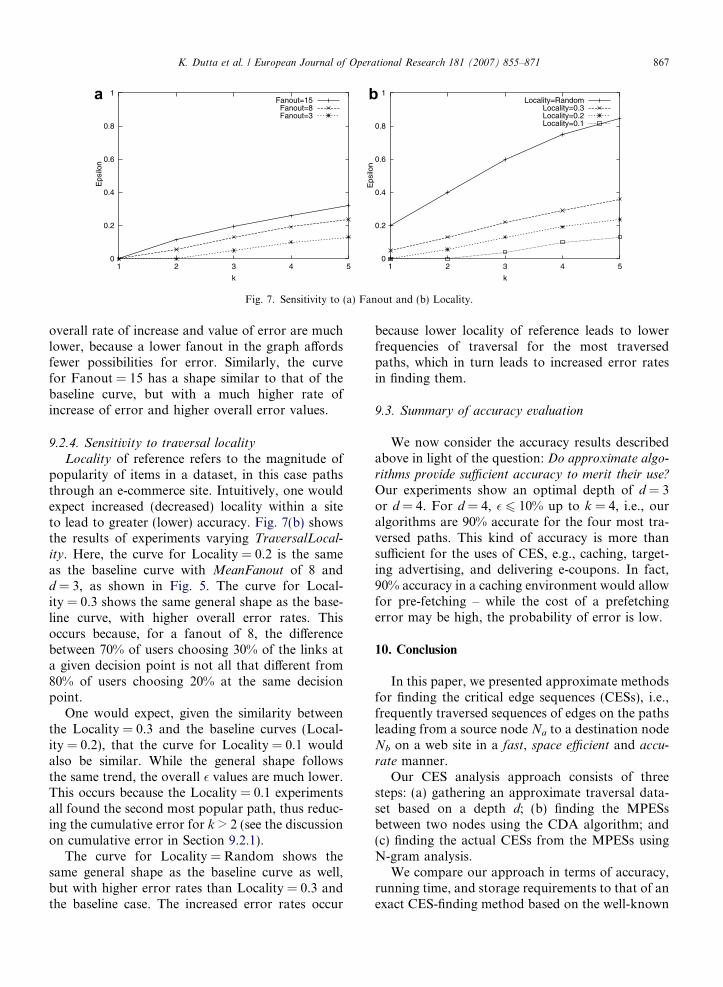
9.2.3. Sensitivity to fanout

Intuitively, one would expect lower (higher) fan-outs to result in higher (lower) accuracy due to thesmaller (larger) number of possible paths throughthe site. Fig. 7(a) shows the results of experimentsvarying fanout f. The curve for Fanout = 8 is thebaseline curve with TraversalLocality of 0.2 andd = 3, shown in Fig. 5. The curve for Fanout = 3is similar in shape to the baseline curve, but the

0

0.2

0.4

0.6

0.8

1

1 2 3 4 5

Eps

ilon

k

Fanout=15Fanout=8Fanout=3

0

0.2

0.4

0.6

0.8

1

1 2 3 4 5

Eps

ilon

k

Locality=RandomLocality=0.3Locality=0.2Locality=0.1

Fig. 7. Sensitivity to (a) Fanout and (b) Locality.


overall rate of increase and value of error are muchlower, because a lower fanout in the graph affordsfewer possibilities for error. Similarly, the curvefor Fanout = 15 has a shape similar to that of thebaseline curve, but with a much higher rate ofincrease of error and higher overall error values.

9.2.4. Sensitivity to traversal locality

Locality of reference refers to the magnitude ofpopularity of items in a dataset, in this case pathsthrough an e-commerce site. Intuitively, one wouldexpect increased (decreased) locality within a siteto lead to greater (lower) accuracy. Fig. 7(b) showsthe results of experiments varying TraversalLocal-

ity. Here, the curve for Locality = 0.2 is the sameas the baseline curve with MeanFanout of 8 andd = 3, as shown in Fig. 5. The curve for Local-ity = 0.3 shows the same general shape as the base-line curve, with higher overall error rates. Thisoccurs because, for a fanout of 8, the differencebetween 70% of users choosing 30% of the links ata given decision point is not all that different from80% of users choosing 20% at the same decisionpoint.

One would expect, given the similarity betweenthe Locality = 0.3 and the baseline curves (Local-ity = 0.2), that the curve for Locality = 0.1 wouldalso be similar. While the general shape followsthe same trend, the overall � values are much lower.This occurs because the Locality = 0.1 experimentsall found the second most popular path, thus reduc-ing the cumulative error for k > 2 (see the discussionon cumulative error in Section 9.2.1).

The curve for Locality = Random shows thesame general shape as the baseline curve as well,but with higher error rates than Locality = 0.3 andthe baseline case. The increased error rates occur

because lower locality of reference leads to lowerfrequencies of traversal for the most traversedpaths, which in turn leads to increased error ratesin finding them.

9.3. Summary of accuracy evaluation

We now consider the accuracy results describedabove in light of the question: Do approximate algo-

rithms provide sufficient accuracy to merit their use?

Our experiments show an optimal depth of d = 3or d = 4. For d = 4, � 6 10% up to k = 4, i.e., ouralgorithms are 90% accurate for the four most tra-versed paths. This kind of accuracy is more thansufficient for the uses of CES, e.g., caching, target-ing advertising, and delivering e-coupons. In fact,90% accuracy in a caching environment would allowfor pre-fetching – while the cost of a prefetchingerror may be high, the probability of error is low.

10. Conclusion

In this paper, we presented approximate methodsfor finding the critical edge sequences (CESs), i.e.,frequently traversed sequences of edges on the pathsleading from a source node Na to a destination nodeNb on a web site in a fast, space efficient and accu-

rate manner.Our CES analysis approach consists of three

steps: (a) gathering an approximate traversal data-set based on a depth d; (b) finding the MPESsbetween two nodes using the CDA algorithm; and(c) finding the actual CESs from the MPESs usingN-gram analysis.

We compare our approach in terms of accuracy,running time, and storage requirements to that of anexact CES-finding method based on the well-known


sequential mining tool, WUM. We find that CDAprovides multiple orders of magnitude improve-ments in runtime and storage requirements overthe full-data approach.

We explore the accuracy of the CDA algorithmusing synthetic datasets, using metrics based onthe familiar IR notions of precision and recall. Inparticular, we are interested in how varying theindependence assumption affects the accuracy ofCDA, as well as CDA’s sensitivity to fanout in thegraph, traversal locality, and depth of conditionalprobability.

Based on our results, we gain the followinginsights: (a) as the value of k increases, the errorin the ith (i <= k) path in the result increases as well,i.e., the error for k = 1 is less than the error fork = 2, and so on; (b) as the depth d of conditionalprobability increases, the error in the resultdecreases; (c) there exists an optimal depth d, withthe best possible tradeoff between cost and accuracy– in our tests, the optimal depth was between d = 3and d = 4, at which we obtained results with accu-racy up to 90%; (d) as the fanout f in the graphincreases, the error in the result increases; and (e)as the locality of reference increases, the error inthe result decreases. Our future plans include mod-ifying our algorithms to support user-defined goalsof frequency/rarity, path properties and the possi-bility of considering traversal sequences spanningmultiple sites.

Appendix

Collecting session information

We gather traversal information for each usertraversal on the site directly, without utilizing theweb server log. For each user click, we store a

Table 5Traversal table

Node 1 Node 2 Node d Node (d + 1

N6 N3 N1 N2

N7 N3 N1 N2

N8 N4 N1 N2

N9 N4 N1 N2

N10 N5 N1 N2

N3 N1 N2 N11

N3 N1 N2 N12

N4 N1 N2 N11

N4 N1 N2 N13

N5 N1 N2 N13

node-id within the user’s session state on the website’s application server infrastructure. We concate-nate node-ids clicks from each user session togetherto form a clickstream of node-ids associated with aparticular session (as described in [12]). For exam-ple, in Fig. 2, user Ua visits nodes N7, N3, N1, N2,and N11. Thus, the session for Ua’s visit can be rep-resented as hN7,N3,N1,N2,N11i.

When a session ends (this point is typically con-figurable on the Web site or can be explicitly identi-fied by user logoff for registered users), the session’sclickstream is stored temporarily in a file, whereeach line of the file represents the traversal informa-tion from a single session (each line representing adifferent user). This representation is significantly

smaller than the web log representation of site activ-

ity. For instance, in the web log representation, eachclick on any given node, e.g., N3, would be an inde-pendent and full entry, containing a timestamp,URL, and the IP address of the request origination,among other information.

From the data in the temporary clickstream file,we extract the edge probability vectors by a simpletwo-step method: (a) we first extract all (d + 1)-length traversal sequences; (b) we then load thesesubsequences and the frequency of traversal overthese subsequences into an AGGREGATE_TRA-VERSAL table. A fragment of this table is shownin Table 5 for depth d = 3, based on traversalsshown in the graph fragment in Fig. 2.

In each tuple of the AGGREGATE_TRA-VERSAL table, we store a (d + 1)-length sequence,as well as two counts associated with each (d + 1)-length edge subsequence, and a probability value.Countd represents the number of traversals of thefirst d nodes in the sequence, while Count(d+1) repre-sents the number of traversals of the entire (d + 1)-length sequence. The Probability field denotes the

) Countd Count(d+1) Probability

1 1 1.01 1 1.01 1 1.02 2 1.01 1 1.03 2 0.673 1 0.333 2 0.673 1 0.331 1 1.0


probability that a user will traverse the edge repre-sented by the values in the Node d and Node(d + 1) fields, given that he has arrived at the nodestored in Node d by traversing the nodes stored inNode 1 and Node 2. We can calculate this probabil-ity by dividing Count(d+1) by Countd. For example,consider the first record in the AGGRE-GATE_TABLE fragment, shown in Table 5. Thistuple indicates the following three facts:

1. a single user has traversed the path hN6,N3,N1i(shown by a Countd value of 1);

2. a single user has traversed the pathhN6,N3,N1,N2i (shown by a Count(d+1) value of1); and

3. if a user traverses the path hN6,N3,N1i, thenhe will navigate to N2 next, with probability1.0 (shown as a probability value of 1.0 inTable 5).

Table 6Characteristics of our dataset

Parameter Average Minimum Maximum

Fanout 8 2 10SessionLength 15 4 20Number of users 300,000 – –Number of nodes 150,000 – –Traversal locality 0.2 – –

Generating the experimental synthetic dataset

We model a web site as a graph G = (V,E). Inour experiments, G consists of jVj nodes and Mean-

Fanout · jVj edges, where MeanFanout is the aver-age number of outgoing edges from a node in thegraph. NumUsers users traverse G, each starting ata node chosen from a uniform distribution acrossall nodes in G. Note that this confers a significantdisadvantage to our algorithms – in the real world,users begin traversing the site at a limited number ofstart nodes (e.g., the home page, and perhaps thefirst-level category pages). Had we used a limitedset of starting nodes in these experiments, our accu-racy results would be significantly better than thosereported here.

0

0.2

0.4

0.6

0.8

1

1 2 3 4 5

Eps

ilon

k


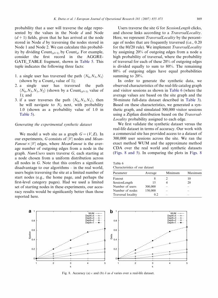
Fig. 8. Accuracy (a) � and (b) d as d

Users traverse the site G for SessionLength clicks,and choose links according to a TraversalLocality.Here, we represent TraversalLocality by the percent-age of nodes that are frequently traversed (i.e., 0.20for the 80/20 rule). We implement TraversalLocality

by assigning 20% of outgoing edges from a node ahigh probability of traversal, where the probabilityof traversal for each of these 20% of outgoing edgesis divided equally to sum to 80%. The remaining80% of outgoing edges have equal probabilitiessumming to 20%.

In order to generate the synthetic data, weobserved characteristics of the real-life catalog graphand visitor sessions as shown in Table 6 (where theaverage values are based on the site graph and the50-minute full-data dataset described in Table 3).Based on these characteristics, we generated a syn-thetic graph, and simulated 300,000 visitor sessionsusing a Zipfian distribution based on the Traversal-

Locality probability assigned to each edge.We first validate the synthetic dataset versus the

real-life dataset in terms of accuracy. Our work witha commercial site has provided access to a dataset of300,000 user sessions across the site. We ran theexact method WUM and the approximate methodCDA over the real world and synthetic datasets(Figs. 8 and 5). In comparing the plots in Figs. 8

0

0.2

0.4

0.6

0.8

1

1 2 3 4 5

Del

ta

k


varies over a real-life dataset.


and 5, we find that the accuracy for our approxi-mate solution for the synthetically-generated datais similar to that of real-life data. Thus, we concludethat our synthetic session log generation accuratelyemulates the real data as far as our approximatealgorithms are concerned. We note here that thetrends of d curves (shown in Fig. 8(b)) closelyresemble those of the trends for � curves inFig. 8(a), for very similar reasons. Thus, we reportonly � results in this paper.

References

[1] R. Agrawal, T. Imielinski, A. Swami, Mining associationrules between sets of items in large databases, in: Proceedingsof the ACM SIGMOD International Conference on Man-agement of Data, May 1993, pp. 207–216.

[2] R. Agrawal, R. Srikant, Fast algorithms for mining associ-ation rules in large databases, in: Proceedings of theInternational Conference on Very Large Databases, 1994,pp. 487–499.

[3] R. Agrawal, R. Srikant, Mining sequential patterns, in:Proceedings of the International Conference on Data Engi-neering, March 1995, pp. 3–14.

[4] R.J. Bayardo, R. Agrawal, Mining the most interesting rules,in: Proceedings of the ACM SIGKDD International Con-ference on Knowledge Discovery and Data Mining, 1999,pp. 145–154.

[5] J. Borges, M. Levene, Data mining of user navigationpatterns, in: Proceedings of the Workshop on Web UsageAnalysis and User Profiling, 1999. Available from: <http://www.acm.org/sigs/sigkdd/proceedings/webkdd99/toconline.htm>.

[6] M.K. Brown, A. Kellner, D. Raggett, Stochastic languagemodels (n-gram) specification(w3c working draft), January2001. Available from: <http://www.w3c.org/TR/ngram-spec/>.

[7] P. Chatterjee, D.H. Hoffman, T.P. Novak, Modeling theclickstream: Implications for web-based advertising efforts,Marketing Science 22 (4) (2003), Fall.

[8] M.-S. Chen, J.S. Park, P.S. Yu, Data mining for pathtraversal patterns in a web environment, in: Proceedings ofthe International Conference on Distributed ComputingSystems, 1996.

[9] K.W. Church, Ngrams, in: Proceedings of the AnnualMeeting of the Association for Computational Linguistics,1995.

[10] T.H. Cormen, C.E. Lieserson, R.L. Rivest, Introduction toAlgorithms, McGraw Hill, 1998.

[11] C.R. Cunha, C.F.B. Jaccoud, Determining www user’s nextaccess and its application to pre-fetching, in: Proceedings ofthe IEEE Symposium on Computers and Communications,July 1997, pp. 6–11.

[12] A. Datta, K. Dutta, D. VanderMeer, K. Ramamritham, S.B.Navathe, An architecture to support scalable online person-alization on the web, VLDB Journal 10 (1) (2001) 104–117.

[13] A. Datta, D. VanderMeer, K. Ramamritham, S. Navathe,Toward a comprehensive model of the content and structure

of, and user interaction over, a web site, in: Proceedings ofthe VLDB Workshop on Technologies for E-Services, Cairo,Egypt, September 2000.

[14] A. Demiriz, webspade: A parallel sequence mining algorithmto analyze web log data, in: Proceedings of the Second IEEEInternational Conference on Data Mining (ICDM, 2002),pp. 755–758, 2002.

[15] A. Demiriz, Asipath: A simple path mining algorithm, in:Proceedings of the 16th International Conference on Paralleland Distributed Computing and Systems (PDCS 2004),November 2004, pp. 9–11.

[16] D. Eppstein, Finding the k shortest paths, SIAM Journal onComputing 28 (1998) 652–673.

[17] D. Florescu, A. Levy, D. Suciu, K. Yagoub, Optimization ofrun-time management of data intensive web sites, in:Proceedings of the VLDB Conference, September 1999, pp.627–638.

[18] W. Gaul, L. Schmidt-Thieme, Mining web navigation pathfragments, in: Proceedings of the WEBKDD Workshop,August 2000.

[19] F. Korn, A. Labrinidis, Y. Kotidis, C. Faloutsos, Quanti-fiable data mining using ratio rules, VLDB Journal (2000)254–266.

[20] H. Kum, J. Pei, W. Wang, D. Duncan, Approxmap:Approximate mining of consensus sequential patterns, in:Proceedings of the SIAM International Conference on DataMining, May 2003.

[21] M.J. Zaki, Spade: An efficient algorithm for mining frequentsequences, Machine Learning Journal 42 (January–Febru-ary) (2001) 31–60.

[22] B. Mosbasher, N. Jain, E. Han, J. Srivastava, Web mining:Pattern discovery from world wide web transactions, Tech-nical Report 96-050, University of Minnesota, Dept. ofComputer Science, Minneapolis, 1996.

[23] A. Nanopoulos, Dimitrios Katsaros, Y. Manolopoulos,Effective prediction of web-user accesses, a data miningapproach, in: Proceedings of the WEBKDD Workshop,August 2001.

[24] J. Pitkow, P. Priolli, Mining longest repeating subsequencesto predict world wide web surfing, in: Proceedings of theUSENIX Symposium on Internet Technologies and Systems,Boulder, Colorado, October 1999.

[25] D.R. Shier, On algorithms for finding the k shortest paths ina network, Networks, 1979.

[26] M. Spiliopoulou, L.S. Faulstich, K. Winkler, A data mineranalyzing the navigational behavior of web users, in:International Conference of Workshop on Machine Learn-ing in User Modelling 1999.

[27] M. Spiliopoulou, C. Pohle, Data mining for measuring andimproving the success of web sites, in: Special Issue onApplications of Data Mining to Electronic Commerce,Journal of Data Mining and Knowledge Discovery 5(January–April) (2001) 85–114.

[28] M. Spilioupoulou, L.C. Faulstich, P. Atzeni, A. Mendelzon,G. Mecca, Wum: A tool for web utilization analysis, in:International Workshop on World Wide Web and Dat-abases, 1998, pp. 184–203.

[29] R. Srikant, R. Agrawal, Mining sequential patterns: Gener-alizations and performance improvements, in: Proceedings ofthe International Conference on Extending Database Tech-nology, March 1996, pp. 3–17.

http://www.acm.org/sigs/sigkdd/proceedings/webkdd99/toconline.htm



http://www.w3c.org/TR/ngram-spec/

http://www.w3c.org/TR/ngram-spec/


[30] A. Throne, Why he who dies with the hottest toy wins,March 2002. Available from: <http://www.brandera.com/features/01/03/14/trendset.html>.

[31] Yahoo! Yahoo media relations: General corporate faq,March 2006. Available from: <http://docs.yahoo.com/docs/info/faq.html>.

[32] M.J. Zaki, N. Lesh, M. Ogihara, Planmine: Sequence miningfor plan failures, in: Proceedings of the InternationalConference on Knowledge Discovery and Data Mining,1998, pp. 369–373.

http://www.brandera.com/features/01/03/14/trendset.html

http://www.brandera.com/features/01/03/14/trendset.html

http://docs.yahoo.com/docs/info/faq.html

http://docs.yahoo.com/docs/info/faq.html

Documents

A fast method for discovering critical edge sequences in e-commerce catalogs