A Fast Gradient Method for Nonnegative SparseRegression with Self Dictionary

Nicolas Gillis∗ Robert Luce†

Abstract

Nonnegative matrix factorization (NMF) can be computed efficiently under the sep-arability assumption, which asserts that all the columns of the input data matrix belongto the convex cone generated by only a few of its columns. The provably most robustmethods to identify these basis columns are based on nonnegative sparse regression andself dictionary, and require the solution of large-scale convex optimization problems. Inthis paper we study a particular nonnegative sparse regression model with self dictio-nary. As opposed to previously proposed models, it is a smooth optimization problemwhere sparsity is enforced through appropriate linear constraints. We show that theEuclidean projection on the set defined by these constraints can be computed efficiently,and propose a fast gradient method to solve our model. We show the effectiveness ofthe approach compared to state-of-the-art methods on several synthetic data sets andreal-world hyperspectral images.

Keywords Nonnegative matrix factorization, separability, sparse regression, self dictio-nary, fast gradient, hyperspectral imaging, pure-pixel assumption.

1 IntroductionGiven a matrix M ∈ Rm,n where each column of M represents a point in a data set, weassume in this paper that each data point can be well approximated using a nonnegativelinear combination of a small subset of the data points. More precisely, we assume thatthere exists a small subset K ⊂ 1, 2, . . . , n of r column indices and a nonnegative matrixH ∈ Rr,n+ such that

M ≈M(:,K)H.

If M is nonnegative, this problem is closely related to nonnegative matrix factorization(NMF) which aims at decomposing M as the product of two nonnegative matrices W ∈ Rm,r+and H ∈ Rr,n+ with r min(m,n) such that M ≈ WH [20]. In the NMF literature, theassumption above is referred to as the separability assumption [3], and the aim is thereforeto finding a particular NMF with W = M(:,K).

There are several applications to solving near-separable NMF, e.g., blind hyperspectralunmixing [4, 23], topic modeling and document classification [19, 2], video summarizationand image classification [8], and blind source separation [6, 7, 22].∗Department of Mathematics and Operational Research, Faculte Polytechnique, Universite de Mons, Rue

de Houdain 9, 7000 Mons, Belgium, (nicolas.gillis@umons.ac.be). NG acknowledges the support of theF.R.S.-FNRS (incentive grant for scientific research no F.4501.16) and of the ERC (starting grant no 679515).†Ecole Polytechnique Federale de Lausanne, Station 8, 1015 Lausanne, Switzerland

(robert.luce@epfl.ch)

1

1.1 Self Dictionary and Sparse Regression based ApproachesMany algorithms have been proposed recently to solve the near-separable NMF problem;see [13] and the references therein. In hyperspectral unmixing, the most widely used al-gorithms sequentially identify important columns of M , such as vertex component analysis(VCA) [24] or the successive projection algorithm (SPA) [1, 17]; see section 4 for more de-tails. Another important class of algorithms for identifying a good subset K of the columnsof M is based on sparse regression and self dictionaries. These algorithms are computation-ally more expensive but have the advantage to consider the selection of the indices in K atonce leading to the most robust algorithms; see the discussion [13].

An exact model for nonnegative sparse regression with self dictionary [9, 8] is

minX≥0

‖X‖row,0 such that ‖M −MX‖ ≤ ε, (1)

where ‖X‖row,0 equals to the number of nonzero rows of X, and ε denotes the noise levelof the data M . Here, the norm in which the residual M − MX is measured should bechosen in dependence of the noise model. It is easy to see that there exists a nonnegativematrix X with r nonzero rows such that M = MX if and only if there exists an index setK of cardinality r and a nonnegative matrix H such that M = M(:,K)H: The index set Kcorresponds to the indices of the nonzero rows of X, and hence we have H = X(K, :).

In [9, 8], the difficult problem (1) is relaxed to the convex optimization problem

minX≥0

‖X‖1,q s.t. ‖M −MX‖ ≤ ε, (2)

where ‖X‖1,q :=∑ni=1‖X(i, :)‖q. In [9], q = +∞ is used while, in [8], q = 2 is used. The

quantity ‖X‖1,q is the `1-norm of the vector containing the `q norms of the rows of X.Because the `1 norm promotes sparsity, this model is expected to generate a matrix X withonly a few nonzero rows. The reason is that the `1 norm is a good surrogate for the `0 normon the `∞ ball. In fact, the `1 norm is the convex envelope of the `0 norm on the `∞ ball,that is, the `1 norm is the largest convex function smaller than the `0 norm on the `∞ ball;see [26]. Hence for q = +∞ and X ≤ 1, we have ‖X‖1,∞ ≤ ‖X‖row,0 so that (2) provides alower bound for (1).

The model (2) was originally proved to be robust to noise, but only at the limit, that is,only for ε → 0, and assuming no columns of M(:,K) are repeated in the data set [9]. If acolumn of M(:,K) is present twice in the data set, the (convex) models cannot discriminatebetween them and might assign a weights on both columns. (The situation is worsened inthe presence of more duplicates and near-duplicates, which is typical in hyperspectral imagedata, for example). More recently, Xu and Ma [10] improved the robustness analysis ofthe model for q = +∞. However, their robustness result is restricted to the case when thecolumns of M(:,K) are not duplicated.

If the input matrix is nonnegative, it can be normalized so that the entries of the columnsof matrix H (hence X) are at most one, as suggested for example in [9]. This can be achievedby normalizing each column of M so that its entries sum to one. After such a normalization,we have for all j

1 = ‖M(:, j)‖1 = ‖MX(:, j)‖1 = ‖∑k

M(:, k)X(k, j)‖1

=∑k∈K

X(k, j)‖M(:, k)‖1 = ‖X(:, j)‖1,

since M and X are nonnegative. If M is normalized, another sparse regression modelproposed in [5] and later improved in [16] is the following:

minX∈Rn,n

+

trace(X) s.t.‖M −MX‖ ≤ εX(i, j) ≤ X(i, i) ≤ 1 ∀i, j.

(3)

2

(The model can easily be generalized for non-normalized M ; see model (5)). Here sparsityis enforced by minimizing the `1 norm of the diagonal of X as trace(X) = ‖diag(X)‖1 forX ≥ 0, while no off-diagonal entry of X can be larger than the diagonal entry in its row.Hence diag(X) is sparse if and only if X is row sparse.

The model (3) is, to the best of our knowledge, the provably most robust for near-separable NMF [16]. In particular, as opposed to most near-separable NMF algorithms thatrequire M(:,K) to be full column rank, it only requires the necessary condition that nocolumn of M(:,K) is contained in the convex hull of the other columns. More precisely, letus define the conical robustness of a matrix W ∈ Rm,r as

κ = min1≤k≤r

minx∈Rr−1

+

‖W (:, k)−W (:, 1, . . . , r \ k)x‖1.

We then say that W is κ-robustly conical, and the following recovery result can be obtained:

Theorem 1 ([16], Th. 7). Let M = M(:,K)H be a separable matrix with M(:,K) beingκ-robustly conical and the entries of each column of H summing to at most one, and letM = M +N . If ε := max1≤j≤n‖N(:, j)‖1 ≤ O

(κr

), then the model (3) allows to recover the

columns of M(:,K) up to error O(r εκ).

This result is stronger than Xu and Ma [10] because it allows duplicated columns; seesection 2 for a discussion.

1.2 Contribution and Outline of the PaperOur contribution is three fold:

• In section 2, we prove that both sparse regression models (2) and (3) are equivalent,provided that X ≤ 1. This significantly improves the theoretical robustness analysisof (2), as the results for (3) directly apply to (2).

• In section 3, we introduce a new model, very similar to (3) (using the Frobeniusnorm, and not assuming normalization of the input data), for which we propose anoptimal first-order method: the key contribution is a very effective and non-trivialprojection onto the feasible set. Although our approach still requires O(n2) operationsper iteration, it can solve larger instances of (3) than commercial solvers, with n ∼1000. We show the effectiveness of our approach on synthetic data sets in section 4.1.

• In section 4.2, we preselect a subset of the columns of the input matrix and scale themappropriately (depending on their importance in the data set) so that we can applyour method meaningfully to real-world hyperspectral images when n ∼ 106. We showthat our approach outperforms state-of-the-art pure pixel search algorithms.

2 Equivalence between Sparse Regression Models (2)and (3)

If we assume that the entries of the matrix X in the model (2) are bounded above by one,which is the case for example in hyperspectral imaging, or if we normalize the columns onthe input matrix M (see section 1), then we can consider the following natural variant ofthe model (2) with an upper bound constraint on X:

min0≤X≤1

‖X‖1,∞ s.t. ‖M −MX‖ ≤ ε. (4)

Theorem 2. Let ‖·‖ be a column wise matrix norm, that is, ‖A‖ =∑i αi‖A(:, i)‖c for some

αi > 0 and some vector norm ‖·‖c. Then (4) is equivalent to (3) in the following sense:

3

• At optimality, both objective functions coincide,

• any optimal solution of (3) is an optimal solution of (4), and

• any optimal solution of (4) can be trivially transformed into an optimal solution of (3).

Proof. Observe that

• Any feasible solution of (3) is a feasible solution of (4): in fact, the only differencebetween the feasible domains are the additional constraints Xij ≤ Xii for all i, j.

• The objective function of (4) is larger than the one of (3): in fact, by definition,trace(X) ≤ ||X||1,∞. Moreover, the two objective functions coincide if and only ifXii = maxj Xij for all i.

These observations imply that the optimal objective function value of (3) is larger thanthe one of (4) (since any feasible solution X of (3) is feasible for (4) and satisfies trace(X) =‖X‖1,∞).

Therefore, if we can transform any optimal solution X∗ of (4) into a feasible solution X†of (3) with the same objective function value, X† will be an optimal solution of (3) and theproof will be complete.

Let X∗ be any optimal solution of (4). If X∗ = 0, then X∗ is trivially feasible for (3)and the proof is complete.

So assume X∗ 6= 0. We will show by contradiction that ‖M −MX∗‖ = ε, so assumeassume that ‖M − MX∗‖ < ε. By continuity of norms there exists 0 < δ < 1 so that‖M −M(δX∗)‖ < ε. The matrix δX∗ is a feasible solution for (4) since 0 ≤ δX∗ ≤ X∗ ≤ 1while ‖δX∗‖1,∞ = δ‖X∗‖1,∞ < ‖X∗‖1,∞, a contradiction to the optimality of X∗.

Assume that X∗ii < X∗ij ≤ 1 for some j. Let us show this is only possible if M(:, i) =MX∗(:, i): assume M(:, i) 6= MX∗(:, i), we have

M(:, i)−MX∗(:, i) = (1−X∗ii)M(:, i)−MX∗(I, i),

where I = 1, . . . , n \ i. Increasing X∗ii to X∗ij while decreasing the entries of X∗(I, i) bythe factor β = X∗ii

X∗ij< 1 decreases ‖M(:, i) −MX(:, i)‖c by a factor (1 −X∗ii) which would

be a contradiction since ‖M −MX‖ would be reduced (see above).Finally, let us construct another optimal solution X†: we take X† = X∗, and for all j

such that X∗ii < X∗ij ≤ 1, X†ii is replaced with X†ij and X†(I, i) is multiplied by the factorβ = X∗ii

X∗ij< 1. The error ‖M −MX‖ remains unchanged while the objective function might

have only decreased: X† is an optimal solution of (4) satisfying X†ii = maxj X†ij hence isalso an optimal solution of (3).

It is interesting to note that the (weaker) robustness result for (2) of Fu and Ma [10,Th. 2] without duplicates is closely related to the robustness result for (3) of [16, Th. 2]where that case is also analyzed separately. We recall the result here for completeness:

Theorem 3 ([16], Th. 2). Let M = M(:,K)H where M(:,K) is κ-robustly conical and wherethe entries of each column of H are at most one. Let also M = M +N and H(i, j) ≤ β < 1for all 1 ≤ i ≤ m and j /∈ K (this is the condition that there is no duplicates of the columnsof M(:,K)). If ε := max1≤j≤n ||N(:, j)||2 < κ(1−β)

20 , then the model (3) allows to recover thecolumns of M(:,K) up to error ε.

The advantage of the formulation (3) is that the objective function is smooth. Moreover,as we will show in Section 3.3, projecting onto the feasible set can be made efficiently (evenwhen the model is generalized to the case where the columns of the input matrix are notnormalized). Hence, we will be able to apply an optimal first order method of smooth convexoptimization with faster convergence rate to this problem.

4

3 Convex Model without Normalization and Fast Gra-dient Method

The model (3) can be generalized in case the entries of each column of H do not necessarilysum to one, where M = M(: K)H, without column normalization of M . The advantage istwofold: column normalization (i) is only possible for nonnegative input matrix, and (ii) mayintroduce distortion in the data set as it would be equivalent to consider that the noise addedto each data point (that is, each column of M) is proportional to it [19]. If one wants toconsider absolute error (the norm of each column of the noise is independent on the normof the input data), then the input matrix should not be normalized and the following modelshould be considered [16]:

minX∈Ω

trace(X) such that ||M −MX||F ≤ ε. (5)

The set Ω is defined as

Ω := X ∈ Rn,n+ | Xii ≤ 1, wiXij ≤ wjXii∀i, j, (6)

where the vector w ∈ Rn+ are the column `1 norms of M , that is, wj = ‖M(:, j)‖1 for all j.The upper bounds Xij ≤ wj

wiXii come from the fact that each weight used to reconstruct a

data point inside the convex cone generated by some extreme rays cannot exceed the ratioof the `1 norm of that data point to each individual extreme ray.

Note that the optimization problem (5) is convex, and it can be solved as a second orderconic program (SOCP) in n2 variables. This large number of variables even for moderatevalues of n rules out the use of off-the-shelf SOCP optimization software. In this section,we describe an optimal first-order method to solve (5). A main contribution is in the (non-trivial) projection onto the feasible set Ω.

3.1 Related WorkTo solve a model similar to (3), Bittorf et al. [5] used a stochastic subgradient descentmethod, with a non-smooth objective function (they were using the component-wise `1norm of M −MX). Although the cost per iteration is relatively low with O(n2) operationsper iterations, the convergence is quite slow.

To solve (2) with q = +∞ in [9] and q = 2 in [8], authors propose an alternating directionmethod of multipliers (ADMM). However, ADMM is not an optimal first-order method asthe objective function converges at rate O(1/k) vs. O(1/k2) for optimal first-order methods,where k is the iteration number. Moreover, the cost per iteration of ADMM is larger asit requires the introduction of new variables (one variable Y of the same dimension as X,Lagrangian multipliers and a parameter which is not always easy to tune).

Another optimal first-order method was proposed in [21]. However, it solves a ratherdifferent optimization problem, namely

minX,Q

pT diag(X) + β‖MX −M −Q‖2F + λ‖Q‖1,

where two regularization parameters have to be tuned while the objective function is non-smooth, so that authors use a local linear approximation approach to smooth the objectivefunction. They also require column normalization while our approach does not. Also, theypoint out that it would be good to incorporate the constraints from (3), which we do in thispaper by developing an effective projection on the feasible set.

3.2 Fast Gradient Method for (5)It is possible to solve (5) using commercial solvers that are usually based on interior-pointmethods, such as GuRoBi. However, it is computationally rather expensive as there areO(n2) variables, where n is the number of columns of M .

5

Moreover, it has to be noted that in the separable NMF case, it is not important toobtain high accuracy solutions: the main information one wants to obtain is which columnsof M are the important ones. Hence it is particularly meaningful in this context to usefirst-order methods (slower convergence but much lower computational cost per iteration).

The additional constraints that allows to take into account the fact that the columns ofM are not normalized makes the feasible set more complicated, but we develop an efficientprojection method, that allows us to design an optimal first-order method (namely, a fastgradient method).

The function we propose to minimize is

minX∈Ω

F (X) = 12‖M −MX‖2F + µpT diag(X), (7)

where M ∈ Rm,n is the input data matrix, X ∈ Ω are the basis reconstruction coefficientsand p ∈ Rn is a randomly chosen vector that discriminates between (approximate) duplicatebasis vectors present in the data. The parameter µ ∈ R+ acts as a Lagrangean multiplier.

Our goal is to derive computationally efficient schemes to minimize the function F (X)over Ω using first-order optimization approaches. Algorithm 1 describes an optimal first-order method to solve this problem.

Algorithm 1 Fast Gradient Method for Nonnegative Sparse Regression with Self Dictionary(FGNSR)Require: A matrix M ∈ Rm,n, number r of columns to extract, a vector p ∈ Rn++ whose en-

tries are close to 1, a penalty parameter µ, and maximum number of iterations maxiter.Ensure: An set K ⊂ 1, . . . , n of column indices such that minH≥0 ||M −M(:,K)X||F is

small.1: Initialization2: α0 ← 0.05; Y ← 0n,n; X ← Y ; L← σmax(M)2;3: for k = 1 : maxiter do4: Yp ← Y ;5: ∇F (X)←MTMX −MTM + µdiag(p);6: Projection on Ω; see Section 3.37: Y ← PΩ

(X − 1

L∇F (X));

8: X ← Y + βk(Y − Yp), where βk = αk−1(1−αk−1)α2

k−1+αksuch that αk ≥ 0 and α2

k =(1− αk)α2

k−1;9: end for

10: K ← postprocess(X,r); The simplest way is to pick the r largest entries of diag(X) asdone in [5]. In the presence of (near-)duplicated columns of M , one should use moresophisticated strategies [16].

Note that, because M is not necessarily full rank (in particular rank(M) ≤ r when M isa r-separable matrix without noise), the objective function of (7) is not necessarily stronglyconvex. However, its gradient is Lipschitz continuous with constant L = λmax(MTM) =σmax(M)2 and Algorithm 1 is an optimal first-order method for this class of problems,referred to as a fast gradient method, or Nesterov’s method. These methods guarantee thatthe difference between the objective function value at the kth iteration and the optimalobjective function value converges to zero in O

( 1k2

); see [25] and the references therein.

The parameter µ in (7) is crucial as it balances the importance between the approxi-mation error ‖M −MX‖2F and the fact that we want the diagonal of X to be as sparse aspossible. On one hand, if µ is too large, then the term ‖M −MX‖2F will not have muchimportance in the objective function leading to a poor approximation. On the other hand,if µ is too small, then ‖M −MX‖2F will have to be very small and X will be close to theidentity matrix. However, in practice, it seems that the output of Algorithm 1 is not too

6

sensitive to this scaling. The main a reason is that only the largest entries of (the diago-nal of) X will be extracted by the post-processing procedure while the most representativecolumns of M remains the same independently of the value of µ. In other words, increasingµ will have the effect of increasing in average the entries of X but the rows corresponding tothe important columns of M will keep having larger entries. Therefore, the extracted indexset K will remain the same.

To set the value of µ, we propose the following heuristic which appears to work very wellin practice:

• Extract a subset K of r columns of M with the fast algorithm proposed in [17] (otherfast separable NMF algorithms would also be possible);

• Compute the corresponding optimal weight H:

H = argminZ≥0 ||M −M(:,K)Z||2F .

A few iterations of a coordinate descent method were used; see, e.g., [14].

• Define X0(K, :) = H and X0(i, :) = 0 for all i /∈ K.

• Set µ = ‖M−MX0‖2F

pT diag(X0) , to balance the importance of both terms in the objective function.

Note that if the noise level ε, or an estimate thereof, is given as an input, µ can be easilyupdated in the course of the gradient iteration so that ‖M −MX‖F ≈ ε.

3.3 Euclidean Projection on ΩIn Algorithm 1, we need to compute the Euclidean projection of a point X ∈ Rn,n on the setΩ from Equation (6), denoted PΩ. Recall that for a convex subset C ∈ Rn of an Euclideanvector space, a function φ : Rn → C is an Euclidean projection on C if for all x ∈ Rn

‖x− φ(x)‖ = minz∈C‖x− z‖.

We describe in the Appendix how to compute this projection efficiently. More precisely, weshow how to solve the problem minZ∈Ω‖X − F‖F in O(n2 logn) operations. When usingappropriate data structures, the actual computational work can be much less than thisbound suggests, see Remark 2 in the Appendix. For the unweighted case, that is, wj = 1for all 1 ≤ j ≤ n, the projection is similar to the one described in [5], but the inclusion ofnon-unit weights makes the details very much different.

3.4 Computational CostIf the input data matrix M is dense and m ≥ max(r, logn), the computational cost ofAlgorithm 1 is O

(mn2) operations. In fact, analyzing the main steps of Algorithm 1, we

have

Line 2: The maximum singular value of an m-by-n matrix can be well approximated witha few steps of the power method, requiring O (mn) operations.

Line 5: The matrix MTM should be computed only once at a cost of O(mn2) operations.

If m ≥ 2n, then computing (MTM)X requires O(n3) operations. Otherwise, one

should first compute MX at a cost of O(mn2) operations and then MT (MX) at a

cost of O(mn2) operations (the total being smaller than n3 if m ≤ 2n).

Line 7: The projection onto Ω of an n-by-n matrix X requires O(n2 logn

)operations (the

logn factor comes from the fact that we need to sort the entries of each row of X); seeSection 3.3 for the details about the projection step. Note that each row of X can beprojected independently hence this step is easily parallelizable. Moreover, many rowsof X are expected to be all-zeros and their projection is trivial.

7

4 Numerical ExperimentsWe now study the noise robustness of Algorithm 1 numerically, and compare it to severalother state-of-the-art methods for near-separable NMF problems on a number of hyperspec-tral image data sets. We briefly summarize the different algorithms under consideration asfollows.

Successive projection algorithm (SPA). SPA extracts recursively r columns of theinput matrix M . At each step, it selects the column with the largest `2 norm, and projectsall the columns of M on the orthogonal complement of the extracted column [1]. SPA wasshown to be robust to noise [17]. SPA can also be interpreted as a greedy method to solvethe sparse regression model with self dictionary [11].

XRAY. It recursively extracts columns of the input unnormalized matrix M corre-sponding to an extreme ray of the cone generated by the columns of M , and then projectsall the columns of M on the cone generated by the extracted columns. We used the variantreferred to as “max” [19].

Successive nonnegative projection algorithm (SNPA). A variant of SPA usingthe nonnegativity constraints in the projection step [12]. To the best of our knowledge,it is the provably most robust sequential algorithm for separable NMF (in particular, it doesnot need M(: K) to be full rank).

Exact SOCP solution. We solve the exact model (5) using the SOCP solver of GuRoBi1,an interior point method. The obtained solution will serve as a “reference solution”.

FGNSR. An Matlab/C implementation of Algorithm 1, which is publicly available2.In all our experiments with FGNSR and the exact SOCP solution to (5) we use the

simplest postprocessing to extract the sought for index set K from the solution matrix Xin (5): We always pick the indices of the r largest diagonal values of X (see final step inAlgorithm 1).

Table 1 summarizes the following information for the different algorithms: computa-tional cost, memory requirement, parameters, and whether the H is required to be columnnormalized. The FLOP count and memory requirement for the exact soltution of the SOCPvia an interior point method depends on the actual SOCP formulation used, as well as onthe sparsity of the resulting problem. In any case, they are orders of magnitudes greaterthan for the other algorithms.

FLOPs Memory Parameters NormalizationSPA 2mnr + O(mr2) O(mnt) r Yes

XRAY O(mnrt) O(mn) r NoSNPA O(mnrt) O(mn) r Yes

SOCP (GuRoBi, IPM) O(n6) O(n4) ‖N‖F NoFGNSR O(mn2) O(mn+ n2) r or ‖N‖F No

Table 1: Comparison of robust algorithms for near-separable NMF for a dense m-by-n inputmatrix.

In the following section 4.1 we study numerically the noise robustness of the model 5 onan artificial datas et, and in section 4.2 we compare the methods from above to real-worldhyperspectral image data sets.

4.1 Robustness Study on Synthetic DatasetsThe data set we consider is specifically designed to test algorithms for their robustnessagainst noise. We set m = 50, n = 55 and r = 10. Given the noise level ε, a noisy

1https://www.gurobi.com2https://github.com/rluce/FGNSR

8

r-separable matrixM = WH +N ∈ Rm,n (8)

is generated as follows:

• Each entry of the matrix W is generated uniformly at random in the interval [0, 1](using the rand function of Matlab), and each column of W is then normalized sothat it sums to one.

• The first r columns of H are always taken as the identity matrix to satisfy the sep-arability assumption. The remaining r(r−1)

2 = 45 columns of H contain all possiblecombinations of two nonzero entries equal to 0.5 at different positions. Geometrically,this means that these 45 columns of M are the middle points of all the pairs from thecolumns of W .

• No noise is added to the first r columns of M , that is, N(:, j) = 0 for all 1 ≤ j ≤ r,while all the other columns corresponding to the middle points are moved towards theexterior of the convex hull of the columns of W . Specifically, we set

N(:, j) = M(:, j)− w, for r + 1 ≤ j ≤ n,

where w is the average of the columns of W (geometrically, this is the vertex centroidof the convex hull of the columns of W ). Finally, the noise matrix N is scaled so thatit matches the given noise level ‖N‖F = ε.

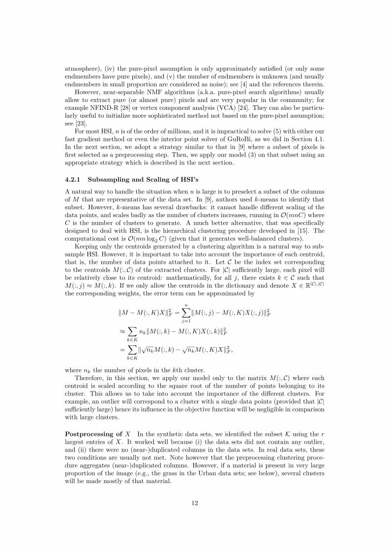
Finally, in order to prevent an artificial bias due to the ordering in which H is constructed,the columns of M are randomly permuted. We give the following illustration of this type ofdata set (with m = r = 3):

0

The shaded area shows the convex hull of W , and the arrow attached to the middle pointsindicate the direction of the noise added to them. With increasing noise level ε, any algorithmfor recovering the conic basis W will eventually be forced to select some displaced middlepoints, and hence will fail to identify W , which makes this data set useful for studying thenoise robustness of such algorithms.

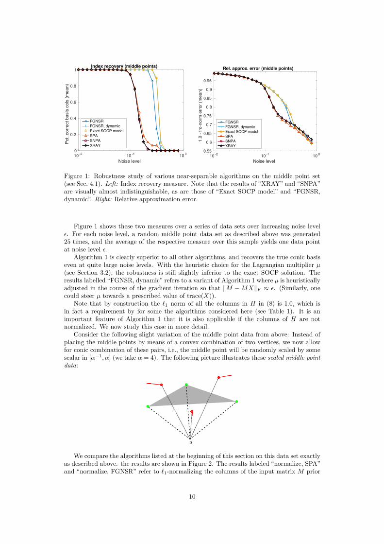
In order to compare the algorithms listed at the beginning of the section, two measuresbetween zero and one will be used, one being the best possible value and zero the worst:given a set of indices K extracted by an algorithm, the measures are as follows:

• Index Recovery. Percentage of entries in K corresponding to columns of W , the originalbasic columns of M .

• Relative approximation error. It is defined as

1.0− minH≥0‖M −M(:,K)H‖F‖M‖F

.

(Taking H = 0 gives a measure of zero).

9

10-2

10-1

100

Noise level

0

0.2

0.4

0.6

0.8

1P

ct. c

orr

ect basis

cols

(m

ean)

Index recovery (middle points)

FGNSR

FGNSR, dynamic

Exact SOCP model

SPA

SNPA

XRAY

10-2

10-1

100

Noise level

0.55

0.6

0.65

0.7

0.75

0.8

0.85

0.9

0.95

1.0

- f

ro-n

orm

err

or

(me

an

)

Rel. approx. error (middle points)

FGNSR

FGNSR, dynamic

Exact SOCP model

SPA

SNPA

XRAY

Figure 1: Robustness study of various near-separable algorithms on the middle point set(see Sec. 4.1). Left: Index recovery measure. Note that the results of “XRAY” and “SNPA”are visually almost indistinguishable, as are those of “Exact SOCP model” and “FGNSR,dynamic”. Right: Relative approximation error.

Figure 1 shows these two measures over a series of data sets over increasing noise levelε. For each noise level, a random middle point data set as described above was generated25 times, and the average of the respective measure over this sample yields one data pointat noise level ε.

Algorithm 1 is clearly superior to all other algorithms, and recovers the true conic basiseven at quite large noise levels. With the heuristic choice for the Lagrangian multiplier µ(see Section 3.2), the robustness is still slightly inferior to the exact SOCP solution. Theresults labelled “FGNSR, dynamic” refers to a variant of Algorithm 1 where µ is heuristicallyadjusted in the course of the gradient iteration so that ‖M −MX‖F ≈ ε. (Similarly, onecould steer µ towards a prescribed value of trace(X)).

Note that by construction the `1 norm of all the columns in H in (8) is 1.0, which isin fact a requirement by for some the algorithms considered here (see Table 1). It is animportant feature of Algorithm 1 that it is also applicable if the columns of H are notnormalized. We now study this case in more detail.

Consider the following slight variation of the middle point data from above: Instead ofplacing the middle points by means of a convex combination of two vertices, we now allowfor conic combination of these pairs, i.e., the middle point will be randomly scaled by somescalar in [α−1, α] (we take α = 4). The following picture illustrates these scaled middle pointdata:

0

We compare the algorithms listed at the beginning of this section on this data set exactlyas described above. the results are shown in Figure 2. The results labeled “normalize, SPA”and “normalize, FGNSR” refer to `1-normalizing the columns of the input matrix M prior

10

10-2

10-1

100

Noise level

0

0.2

0.4

0.6

0.8

1P

ct. c

orr

ect basis

cols

(m

ean)

Index recovery (scaled middle points)

normalize, FGNSR

FGNSR

Exact SOCP model

normalize, SPA

SPA

XRAY

10-2

10-1

100

Noise level

0.65

0.7

0.75

0.8

0.85

0.9

0.95

1

1.0

- f

ro-n

orm

err

or

(me

an

)

Rel. approx. error (scaled middle points)

normalize, FGNSR

FGNSR

Exact SOCP model

normalize, SPA

SPA

XRAY

Figure 2: Robustness study of various near-separable algorithms on the scaled middle pointset (see Sec. 4.1). The show data is analogous to the data in Figure 1. The results for SNPAare not shown here to allow for a cleaner presentation; they are very similar to the ones forSPA.

to applying SPA and FGNSR, respectively. From the results it is clear that FGNSR is byfar the most robust algorithm in this setting.

4.2 Blind Hyperspectral UnmixingA hyperspectral image (HSI) measures the fraction of light reflected (the reflectance) bythe pixels at many different wavelengths, usually between 100 and 200. For example, mostairborne hyperspectral systems measure reflectance for wavelengths between 400nm and2500nm, while regular RGB images contain the reflectance for three visible wavelengths:red at 650nm, green at 550nm and blue at 450nm. Hence, HSI provide much more detailedimages with information invisible to our naked eyes. A HSI can be represented as a nonneg-ative m-by-n matrix where the entry (i, j) of matrix M is the reflectance of the jth pixel atthe ith wavelength, so that each column of M is the so-called spectral signature of a givenpixel. Assuming the linear mixing model, the spectral signature of each pixel equals the lin-ear combination of the spectral signatures of the constitutive materials it contains, referredto as endmembers, where the weights correspond to the abundance of each endmember inthat pixel. This is a simple but natural model widely used in the literature. For example,if a pixel contains 60% of grass and 40% of water, its spectral signature will be 0.6 timesthe spectral signature of the grass plus 0.4 times the spectral signature of water, as 60% isreflected by the grass and 40% by the water. Therefore, we have

M(:, j) =r∑

k=1W (:, k)H(k, j) +N(:, j),

where M(:, j) is the spectral signature of the jth pixel, r is the number of endmembers,W (:, k) is the spectral signature of the kth endmember, H(k, j) is the abundance of thekth endmember in the jth pixel, and N represents the noise (and modeling errors). In thiscontext, the separability assumption is equivalent to the so-called pure-pixel assumptionthat requires that for each endmember there exists a pixel containing only that endmember,that is, for all k, there exists j such that M(:, j) ≈W (:, k).

The theoretical robustness results of near-separable NMF algorithms do not apply inmost cases, the reasons being that (i) the noise level is usually rather high, (ii) imagescontain outliers, (iii) the linear mixing model itself is incorrect (in particular because ofmultiple interactions of the light with the surface, or because of its interaction with the

11

atmosphere), (iv) the pure-pixel assumption is only approximately satisfied (or only someendmembers have pure pixels), and (v) the number of endmembers is unknown (and usuallyendmembers in small proportion are considered as noise); see [4] and the references therein.

However, near-separable NMF algorithms (a.k.a. pure-pixel search algorithms) usuallyallow to extract pure (or almost pure) pixels and are very popular in the community; forexample NFIND-R [28] or vertex component analysis (VCA) [24]. They can also be particu-larly useful to initialize more sophisticated method not based on the pure-pixel assumption;see [23].

For most HSI, n is of the order of millions, and it is impractical to solve (5) with either ourfast gradient method or even the interior point solver of GuRoBi, as we did in Section 4.1.In the next section, we adopt a strategy similar to that in [9] where a subset of pixels isfirst selected as a preprocessing step. Then, we apply our model (3) on that subset using anappropriate strategy which is described in the next section.

4.2.1 Subsampling and Scaling of HSI’s

A natural way to handle the situation when n is large is to preselect a subset of the columnsof M that are representative of the data set. In [9], authors used k-means to identify thatsubset. However, k-means has several drawbacks: it cannot handle different scaling of thedata points, and scales badly as the number of clusters increases, running in O(mnC) whereC is the number of clusters to generate. A much better alternative, that was specificallydesigned to deal with HSI, is the hierarchical clustering procedure developed in [15]. Thecomputational cost is O(mn log2 C) (given that it generates well-balanced clusters).

Keeping only the centroids generated by a clustering algorithm is a natural way to sub-sample HSI. However, it is important to take into account the importance of each centroid,that is, the number of data points attached to it. Let C be the index set correspondingto the centroids M(:, C) of the extracted clusters. For |C| sufficiently large, each pixel willbe relatively close to its centroid: mathematically, for all j, there exists k ∈ C such thatM(:, j) ≈ M(:, k). If we only allow the centroids in the dictionary and denote X ∈ R|C|,|C|the corresponding weights, the error term can be approximated by

‖M −M(:,K)X‖2F =n∑j=1‖M(:, j)−M(:,K)X(:, j)‖2F

≈∑k∈K

nk‖M(:, k)−M(:,K)X(:, k)‖2F

=∑k∈K

‖√nkM(:, k)−

√nkM(:,K)X‖2F ,

where nk the number of pixels in the kth cluster.Therefore, in this section, we apply our model only to the matrix M(:, C) where each

centroid is scaled according to the square root of the number of points belonging to itscluster. This allows us to take into account the importance of the different clusters. Forexample, an outlier will correspond to a cluster with a single data points (provided that |C|sufficiently large) hence its influence in the objective function will be negligible in comparisonwith large clusters.

Postprocessing of X In the synthetic data sets, we identified the subset K using the rlargest entries of X. It worked well because (i) the data sets did not contain any outlier,and (ii) there were no (near-)duplicated columns in the data sets. In real data sets, thesetwo conditions are usually not met. Note however that the preprocessing clustering proce-dure aggregates (near-)duplicated columns. However, if a material is present in very largeproportion of the image (e.g., the grass in the Urban data sets; see below), several clusterswill be made mostly of that material.

12

Therefore, in order to extract a set of column indices from the solution matrix X (seeAlgorithm 1, line 10), we will use a more sophisticated strategy.

The ith row of matrix X provides the weights necessary to reconstruct each column ofM using the ith column of M (since M ≈ MX), while these entries are bounded by thediagonal entry Xii. From this, we note that

(i) If the ith row corresponds to an outlier, it will in general have its corresponding diagonalentry Xii non-zero but the other entries will be small (that is, Xij j 6= i). Therefore, itis important to also take into account off-diagonal entries of X in the postprocessing:a row with a large norm will correspond to an endmember present in many pixels. (Asimilar idea was already proposed in [17, Section 3].)

(ii) Two rows of X that are close to one another (up to a scaling factor) correspond to twoendmembers that are present in the same pixels in the same proportions. Therefore,it is likely that these two rows correspond to the same endmember. Since we wouldlike to identify columns of M that allow to reconstruct as many pixels as possible, weshould try to identify rows of X that are as different as possible. This will in particularallow us to avoid extracting near-duplicated columns.

Finally, we need to identify rows (i) with large norms (ii) that are as different as oneanother as possible. This can be done using SPA on XT : at each step, identify the rowof X with the largest norm and project the other rows on its orthogonal complement (thisis nothing but a QR-factorization with column pivoting). We observe in practice that thispostprocessing is particularly effective at avoiding outliers and near-duplicated columns(moreover, it is extremely fast).

4.2.2 Experimental Set up

In the following sections, we combine the hierarchical clustering procedure with our near-separable NMF algorithm and compare it with state-of-the-art pure-pixel search algorithms(namely SPA, VCA, SNPA, H2NMF and XRAY) on several HSI’s. We have included vertexcomponent analysis (VCA) [24] because it is extremely popular in the hyperspectral unmix-ing community, although it is not robust to noise [17]. VCA is similar to SPA except that(i) it first performs dimensionality reduction of the data using PCA to reduce the ambientspace to dimension r, and (ii) selects the column maximizing a randomly generated linearfunction.

Because the clustering procedure already does some work to identify candidate purepixels, it could be argued that the comparison between our hybrid approach and plain pure-pixel search algorithms is unfair. Therefore, we will also apply SPA, VCA, XRAY, H2NMFand SNPA on the subsampled data set. We subsample the data set by selecting 100 (resp.500) pixels using H2NMF, and denote the corresponding algorithms SPA-100 (resp. SPA-500), VCA-100 (resp. VCA-500), etc.

Because it is difficult to assess the quality of a solution on a real-world HSI, we use therelative error in percent: given the index set K extracted by an algorithm, we report

100minH≥0‖M −M(:,K)H‖F‖M‖F

,

where M is always the full data set.The Matlab code used in this study is available3, and all computations were carried

out with Matlab-R2015b on a standard Linux/Intel box.

4.2.3 Data Sets and Results

We will compare the different algorithms on the following data sets:3https://sites.google.com/site/nicolasgillis/

13

• The Urban HSI4 is taken from HYper-spectral Digital Imagery Collection Experiment(HYDICE) air-borne sensors, and contains 162 clean spectral bands where each imagehas dimension 307× 307. The corresponding near-separable nonnegative data matrixM therefore has dimension 162 by 94249. The Urban data is mainly composed of 6types of materials: road, dirt, trees, roofs, grass and metal (as reported in [18]).

• The San Diego airport HSI is also from the HYDICE air-borne sensors. It contains158 clean bands, with 400×400 pixels for each spectral image hence M ∈ R160000×158

+ .There are about eight types of materials: three road surfaces, two roof tops, trees,grass and dirt; see, e.g., [15].

• The Terrain HSI data set is constituted of 166 clean bands, each having 500 × 307pixels, and is composed of about 5 different materials: road, tree, bare soil, thin andtick grass5.

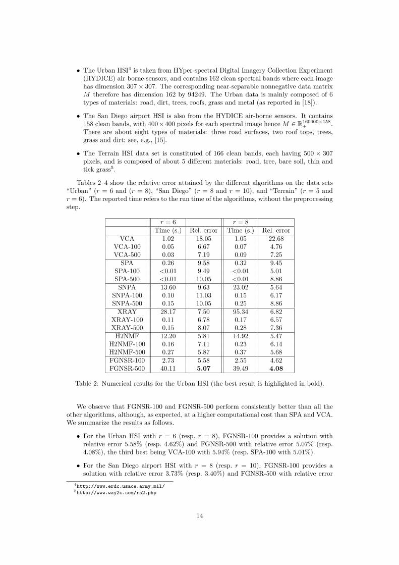
Tables 2–4 show the relative error attained by the different algorithms on the data sets“Urban” (r = 6 and (r = 8), “San Diego” (r = 8 and r = 10), and “Terrain” (r = 5 andr = 6). The reported time refers to the run time of the algorithms, without the preprocessingstep.

r = 6 r = 8Time (s.) Rel. error Time (s.) Rel. error

VCA 1.02 18.05 1.05 22.68VCA-100 0.05 6.67 0.07 4.76VCA-500 0.03 7.19 0.09 7.25

SPA 0.26 9.58 0.32 9.45SPA-100 <0.01 9.49 <0.01 5.01SPA-500 <0.01 10.05 <0.01 8.86SNPA 13.60 9.63 23.02 5.64

SNPA-100 0.10 11.03 0.15 6.17SNPA-500 0.15 10.05 0.25 8.86

XRAY 28.17 7.50 95.34 6.82XRAY-100 0.11 6.78 0.17 6.57XRAY-500 0.15 8.07 0.28 7.36

H2NMF 12.20 5.81 14.92 5.47H2NMF-100 0.16 7.11 0.23 6.14H2NMF-500 0.27 5.87 0.37 5.68FGNSR-100 2.73 5.58 2.55 4.62FGNSR-500 40.11 5.07 39.49 4.08

Table 2: Numerical results for the Urban HSI (the best result is highlighted in bold).

We observe that FGNSR-100 and FGNSR-500 perform consistently better than all theother algorithms, although, as expected, at a higher computational cost than SPA and VCA.We summarize the results as follows.

• For the Urban HSI with r = 6 (resp. r = 8), FGNSR-100 provides a solution withrelative error 5.58% (resp. 4.62%) and FGNSR-500 with relative error 5.07% (resp.4.08%), the third best being VCA-100 with 5.94% (resp. SPA-100 with 5.01%).

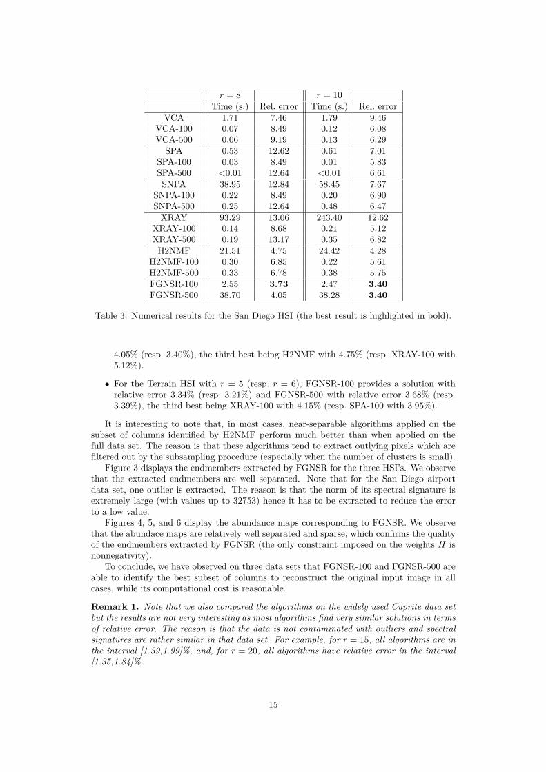
• For the San Diego airport HSI with r = 8 (resp. r = 10), FGNSR-100 provides asolution with relative error 3.73% (resp. 3.40%) and FGNSR-500 with relative error

4http://www.erdc.usace.army.mil/5http://www.way2c.com/rs2.php

14

r = 8 r = 10Time (s.) Rel. error Time (s.) Rel. error

VCA 1.71 7.46 1.79 9.46VCA-100 0.07 8.49 0.12 6.08VCA-500 0.06 9.19 0.13 6.29

SPA 0.53 12.62 0.61 7.01SPA-100 0.03 8.49 0.01 5.83SPA-500 <0.01 12.64 <0.01 6.61SNPA 38.95 12.84 58.45 7.67

SNPA-100 0.22 8.49 0.20 6.90SNPA-500 0.25 12.64 0.48 6.47

XRAY 93.29 13.06 243.40 12.62XRAY-100 0.14 8.68 0.21 5.12XRAY-500 0.19 13.17 0.35 6.82

H2NMF 21.51 4.75 24.42 4.28H2NMF-100 0.30 6.85 0.22 5.61H2NMF-500 0.33 6.78 0.38 5.75FGNSR-100 2.55 3.73 2.47 3.40FGNSR-500 38.70 4.05 38.28 3.40

Table 3: Numerical results for the San Diego HSI (the best result is highlighted in bold).

4.05% (resp. 3.40%), the third best being H2NMF with 4.75% (resp. XRAY-100 with5.12%).

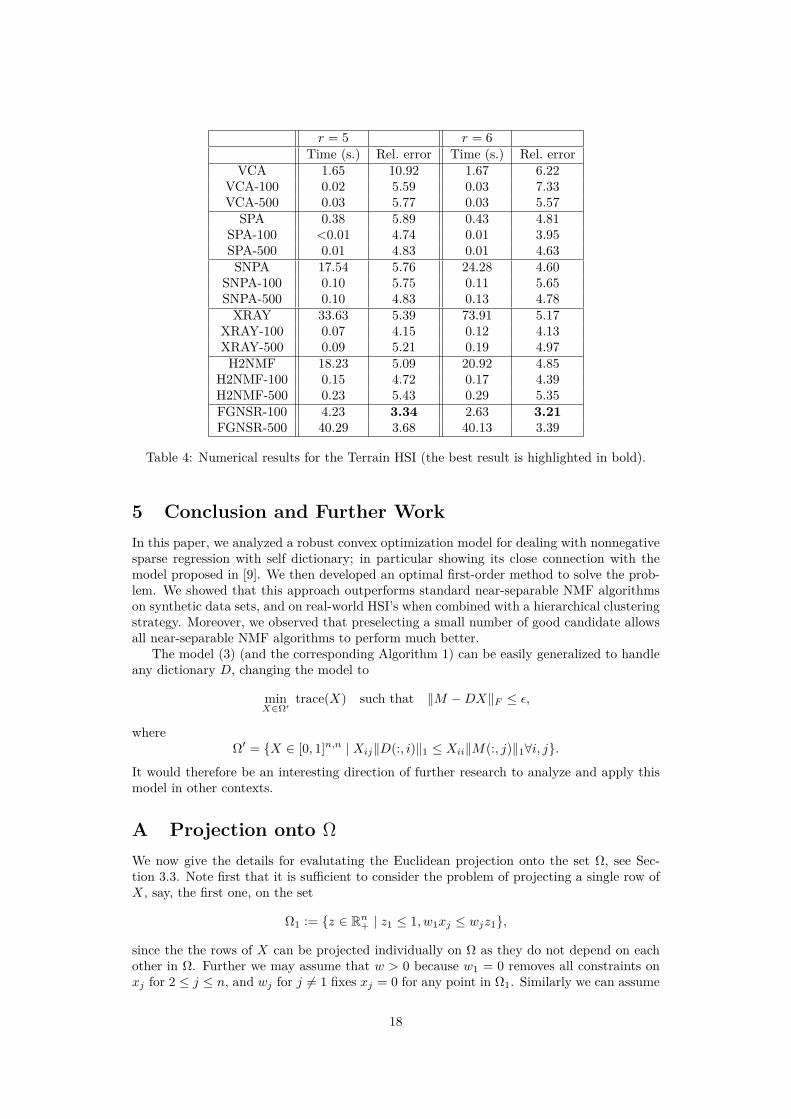
• For the Terrain HSI with r = 5 (resp. r = 6), FGNSR-100 provides a solution withrelative error 3.34% (resp. 3.21%) and FGNSR-500 with relative error 3.68% (resp.3.39%), the third best being XRAY-100 with 4.15% (resp. SPA-100 with 3.95%).

It is interesting to note that, in most cases, near-separable algorithms applied on thesubset of columns identified by H2NMF perform much better than when applied on thefull data set. The reason is that these algorithms tend to extract outlying pixels which arefiltered out by the subsampling procedure (especially when the number of clusters is small).

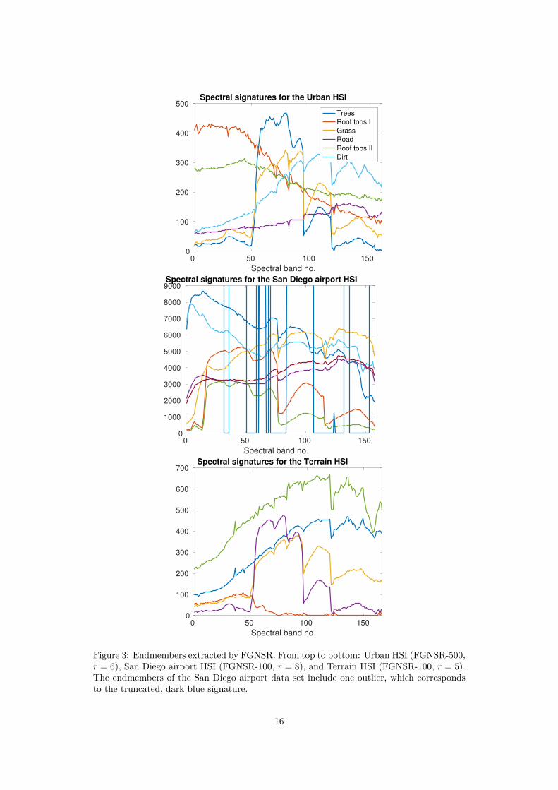
Figure 3 displays the endmembers extracted by FGNSR for the three HSI’s. We observethat the extracted endmembers are well separated. Note that for the San Diego airportdata set, one outlier is extracted. The reason is that the norm of its spectral signature isextremely large (with values up to 32753) hence it has to be extracted to reduce the errorto a low value.

Figures 4, 5, and 6 display the abundance maps corresponding to FGNSR. We observethat the abundace maps are relatively well separated and sparse, which confirms the qualityof the endmembers extracted by FGNSR (the only constraint imposed on the weights H isnonnegativity).

To conclude, we have observed on three data sets that FGNSR-100 and FGNSR-500 areable to identify the best subset of columns to reconstruct the original input image in allcases, while its computational cost is reasonable.

Remark 1. Note that we also compared the algorithms on the widely used Cuprite data setbut the results are not very interesting as most algorithms find very similar solutions in termsof relative error. The reason is that the data is not contaminated with outliers and spectralsignatures are rather similar in that data set. For example, for r = 15, all algorithms are inthe interval [1.39,1.99]%, and, for r = 20, all algorithms have relative error in the interval[1.35,1.84]%.

15

0 50 100 150

Spectral band no.

0

100

200

300

400

500Spectral signatures for the Urban HSI

Trees

Roof tops I

Grass

Road

Roof tops II

Dirt

0 50 100 150

Spectral band no.

0

1000

2000

3000

4000

5000

6000

7000

8000

9000Spectral signatures for the San Diego airport HSI

0 50 100 150

Spectral band no.

0

100

200

300

400

500

600

700Spectral signatures for the Terrain HSI

Figure 3: Endmembers extracted by FGNSR. From top to bottom: Urban HSI (FGNSR-500,r = 6), San Diego airport HSI (FGNSR-100, r = 8), and Terrain HSI (FGNSR-100, r = 5).The endmembers of the San Diego airport data set include one outlier, which correspondsto the truncated, dark blue signature.

16

Figure 4: Abundance maps corresponding to the endmembers extracted by FGNSR-500 forthe Urban HSI (r = 6). From left to right, top to bottom: (i) trees, (ii) roof tops I, (iii) grass,(iv) road, (v) roof tops II, (vi) dirt.

Figure 5: Abundance maps corresponding to the endmembers extracted by FGNSR-100for the San Diego airport HSI (r = 8). From left to right, top to bottom: (i) roof topsI, (ii) grass, (iii) dirt, (iv) road surface I, (v) trees, (vi) roof tops II, (vii) road surface I,(viii) outlier.

17

r = 5 r = 6Time (s.) Rel. error Time (s.) Rel. error

VCA 1.65 10.92 1.67 6.22VCA-100 0.02 5.59 0.03 7.33VCA-500 0.03 5.77 0.03 5.57

SPA 0.38 5.89 0.43 4.81SPA-100 <0.01 4.74 0.01 3.95SPA-500 0.01 4.83 0.01 4.63SNPA 17.54 5.76 24.28 4.60

SNPA-100 0.10 5.75 0.11 5.65SNPA-500 0.10 4.83 0.13 4.78

XRAY 33.63 5.39 73.91 5.17XRAY-100 0.07 4.15 0.12 4.13XRAY-500 0.09 5.21 0.19 4.97

H2NMF 18.23 5.09 20.92 4.85H2NMF-100 0.15 4.72 0.17 4.39H2NMF-500 0.23 5.43 0.29 5.35FGNSR-100 4.23 3.34 2.63 3.21FGNSR-500 40.29 3.68 40.13 3.39

Table 4: Numerical results for the Terrain HSI (the best result is highlighted in bold).

5 Conclusion and Further WorkIn this paper, we analyzed a robust convex optimization model for dealing with nonnegativesparse regression with self dictionary; in particular showing its close connection with themodel proposed in [9]. We then developed an optimal first-order method to solve the prob-lem. We showed that this approach outperforms standard near-separable NMF algorithmson synthetic data sets, and on real-world HSI’s when combined with a hierarchical clusteringstrategy. Moreover, we observed that preselecting a small number of good candidate allowsall near-separable NMF algorithms to perform much better.

The model (3) (and the corresponding Algorithm 1) can be easily generalized to handleany dictionary D, changing the model to

minX∈Ω′

trace(X) such that ‖M −DX‖F ≤ ε,

whereΩ′ = X ∈ [0, 1]n,n | Xij‖D(:, i)‖1 ≤ Xii‖M(:, j)‖1∀i, j.

It would therefore be an interesting direction of further research to analyze and apply thismodel in other contexts.

A Projection onto ΩWe now give the details for evalutating the Euclidean projection onto the set Ω, see Sec-tion 3.3. Note first that it is sufficient to consider the problem of projecting a single row ofX, say, the first one, on the set

Ω1 := z ∈ Rn+ | z1 ≤ 1, w1xj ≤ wjz1,

since the the rows of X can be projected individually on Ω as they do not depend on eachother in Ω. Further we may assume that w > 0 because w1 = 0 removes all constraints onxj for 2 ≤ j ≤ n, and wj for j 6= 1 fixes xj = 0 for any point in Ω1. Similarly we can assume

18

Figure 6: Abundance maps corresponding to the endmembers extracted by FGNSR-100for the Terrain HSI (r = 7). From left to right, top to bottom: (i) roads I, (ii) roads II,(iii) grass, (iv) trees, (v) roads III.

w.l.o.g. that xj > 0 for 2 ≤ j ≤ n, since xj ≤ 0 fixes zj = 0 for any point in Ω1 and doesnot affect the choice of the first coordinate. Note that the norm we wish to minimize nowis given by the standard Euclidean norm ‖x‖ = (

∑j x

2j )

12 .

Let t ∈ R be a parameter and denote by φt : Rn → Rn the mapping

φt(x)j :=

t if j = 1,wj

w1t if j 6= 1 and w1

wjxj ≥ t,

xj else.(9)

From the definition we see that for all x ∈ Rn and all t ∈ [0, 1] we have that φt(x) ∈ Ω1.Unfortunately we cannot simply assume that 0 ≤ x1 ≤ 1. Treating the cases x1 < 0, 0 ≤

x1 ≤ 1 and 1 < x1 homogeneously puts a burden on the notation and slightly obfuscates thearguments used in the following. We set x+

1 := min1,max0, x1 and x−1 := min0, x1.

Lemma 1. Let x ∈ Rn, then

minz∈Ω1‖x− z‖ = min

t∈[x+1 ,1]‖x− φt(x)‖.

In particular, if z∗ = argminz∈Ω1‖x− z‖, we have for 2 ≤ j ≤ n that

w1z∗j < wjz

∗1 if w1xj < wjz

∗1

and

w1z∗j = wjz

∗1 if w1xj ≥ wjz∗1 .

Proof. Let z∗ = argminz∈Ω1 . We will show first that

minz∈Ω1‖x− z‖ = min

t∈[0,1]‖x− φt(x)‖.

If w1xj < wjz∗1 , it follows z∗j = xj , because only in this case the cost contribution of

the j-th coordinate is minimum (zero). Otherwise, if w1xj ≥ wjz∗1 , the projection cost fromthe j-th coordinate is minimized only if xj = wj

w1z∗1 , because all the quantities involved are

positive. It follows that z∗j = φz∗1 (x)j for 2 ≤ j ≤ n. And since z∗1 ∈ [0, 1], it follows thatz∗ = argmint∈[0,1]‖x− φt(x)‖.

To finish the proof, we will now show that z∗1 ≥ x+1 , which is trivial for the case x1 < 0.

In the case x1 ∈ [0, 1], we show z∗1 ≥ x1. In order to obtain a contradiction, assume z∗1 < x1,and define z ∈ Ω1 by

zj =x1 if j = 1z∗j if j 6= 1.

19

We compute

‖x− z‖2 =n∑j=1

(xj − zj)2 =n∑j=2

(xj − z∗j )2 <

n∑j=1

(xj − z∗j )2

= ‖x− z∗‖2,

which contradicts the optimality of z∗.In the case x1 > 1, a similar reasoning shows that z∗1 ≥ 1 (in fact z∗1 = 1).

The previous lemma shows that the optimal projection can be computed by minimizationof a univariate function. We will show next that this can be done quite efficient. For a givenx ∈ Rn we define the function

cx : [x−1 ,∞[→ R, t 7→ ‖x− φt(x)‖2.

By Lemma 1, the (squared) minimum projection cost is given by the minimum of cx|[x+1 ,1],

and our next step is to understand the behavior of cx (see Fig. 7).In order to simplify the notation in the following, we abbreviate bj := w1

wjxj and assume

that the components of x are ordered so that b2 ≤ b3 ≤ · · · ≤ bn, and since xj > 0 for2 ≤ j ≤ n, we have in fact that

x−1 =: b1 ≤ 0 < b2 ≤ b3 ≤ · · · ≤ bn. (10)

Lemma 2. Let x ∈ Rn.(i) The function cx is a piecewise C∞ function with C1 break points bj, and each piece

cx|[bk,bk+1] is strongly convex. In particular, cx is strongly convex and attains its min-imum.

(ii) Let t∗ = argmint∈[x−1 ,∞[ cx(t), the optimal projection of x on Ω1 is

argminz∈Ω1‖x− z‖ =

φx+

1(x) if t∗ < x+

1 ,

φt∗(x) if t∗ ∈ [x+1 , 1] or

φ1(x) if 1 < t∗.

(11)

Proof. We show (i) first. Using the definition (9), we compute for x ∈ Rn and t ∈ [b1,∞[

cx(t) = ‖x− φt(x)‖2 = (x1 − t)2 +∑j∈B(t)

(xj − wj

w1t)2,

whereB(t) := 1 ≤ j ≤ n | t ≤ bj,

from which we see that cx is piecewise smooth and continuously differentiable at the pointsbj . For a point t ∈]bk, bk+1[, we see that c′′x(t) > 0 which shows strong convexity on eachpiece. But c′x is continuous at each bj , so cx is strongly convex on all of [b1,∞[. Finally,since limt→∞ cx(t) = limt→∞(x1 − t)2 =∞, we see see that cx attains its minimum.

The assertions in (ii) follow directly from Lemma 1 and the convexity of cx.

Since cx attains its minimum at t∗ ∈ [b1,∞[, we have that either t∗ ∈ [b1, b2], t∗ ∈]bk, bk+1], for some 2 ≤ k < n, or t∗ ∈]bn,∞[. By the definition of φt, the constraintsw1xj ≤ wjx1 corresponding to break points bj ≥ t∗ are “active” at the point φt∗(x), while allother constraints are not active. More formally, in each of the cases in (12), we can uniquelyassociate a set of optimal active indices B∗ ⊆ 2, . . . , n as follows (here 2 ≤ k ≤ n− 1):

B∗ =

B1 := 2, . . . , n iff t∗ ∈ [b1, b2] =: T1

Bk := k + 1, . . . , n iff t∗ ∈]bk, bk+1] =: TkBn := ∅ iff t∗ ∈]bn,∞[=: Tn.

(12)

20

0 0.2 0.4 0.6 0.8 1

t

0.5

0.6

0.7

0.8

0.9

1

1.1

1.2

1.3

cx(t

)

t6

t5 t

4

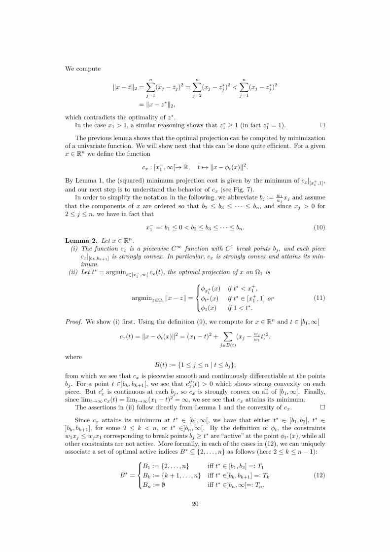
Figure 7: Example for the minimization of cx (n = 6). Black squares indicate the breakpoints and the discs show the location of the trial values tk from (13). The optimal projectionis realized by t4 and the set of optimal active indices are the two break points to the rightof t4.

The preceding observation yields an efficient “dual” algorithm for minimizing cx over[b1,∞[, which we develop in the following lemma.

Lemma 3. Let x ∈ Rn, and t∗ = argmint∈[b1,∞[‖x−φt(x)‖, denote the set of active indicescorresponding to t∗ by B∗ = 1 ≤ j ≤ n | bj ≥ t∗, and set

tk = w1w1x1 +

∑j∈Bk

wjxj

w21 +

∑j∈Bk

w2j

, 1 ≤ k ≤ n. (13)

If tk ∈ Tk, then t∗ = tk (and B∗ = Bk).

Proof. Let 1 ≤ k ≤ n. In order to minimize the strongly convex function

cx(t) = (x1 − t)2 +∑j∈Bk

(xj − wj

w1t)2,

one simply solves c′x(t) = 0 for t, and obtains expression (13). So tk is the minimum of cxunder the hypothesis that Bk is the correct guess for B∗. But by (12) we have that Bk = B∗

if, and only if, tk ∈ Tk, which gives a trivially verifiable criterion for deciding whether theguess for B∗ is correct.

The algorithmic implication of this lemma is as follows. Since we know that one of thesets B1, . . . , Bn must be the optimal active set B∗, we simply compute for each such set Bkthe corresponding optimal point from (13) until we encounter a point tk ∈ Tk, which thenis the sought optimum.

Theorem 4. The Euclidean projection of X ∈ Rn,n on Ω can be computed in O(n2 logn

).

Proof. The projection cost for each row of X amounts to evaluating (13) for each of the setsBk until the optimal set of active indices is identified. If the sets Bk are processed in theordering Bn, Bn−1, . . . , B1, the nominator and denominator in (13) can be updated fromone set to the next, resulting in a computation linear in n. The only non-linear cost per rowis induced by sorting the break points of cx as in (10), which can be done in O (n logn), andresults in the stated worst-case complexity bound.

The function cx is shown in Fig. 7 for a randomly chosen vector x and weights w. Inthis example, the sets B6, B5 and B4 are tested for optimality; the corresponding values tkare indicated in the plot.

21

Remark 2. In an implementation of the outlined algorithm it is not necessary to sort allthe break points of cx for a row x of X as in (10). Only the break points bj ∈ [x+

1 , 1] needto be considered, as all other break points are either never (if bj < x+

1 ) or always (if bj > 1)in the optimal set B∗ of active indices. Denote k1 the number of break points in [x+

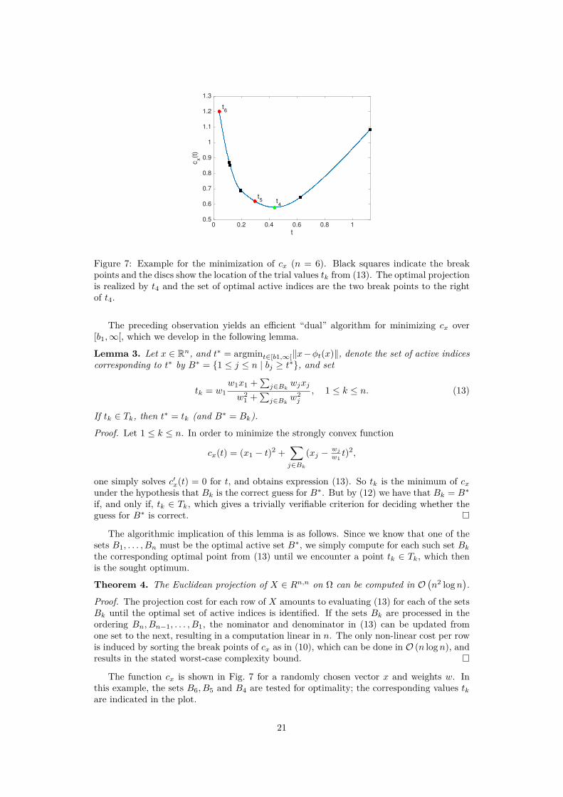
1 , 1] andk2 := |B∗|. If the indices are not sorted but maintained on a heap (see, e.g., [27]), the costoverhead for sorting is reduced to O (k1 log k2). Hence the overall complexity for projectinga single row is O (n+ k1 log k2). The resulting algorithm is sketched in Algorithm 2.

Algorithm 2 Euclidean projection on Ω1Require: x ∈ Rn with x2, . . . , xn > 0, 0 < w ∈ Rn, heap data structure hEnsure: z ∈ Ω1 with ‖x− z‖2 minimal

1: x+1 ← max0, x1

2: B ← 2 ≤ j ≤ n | x+1 ≤ w1

wjxj ≤ 1

3: B∗ ← 2 ≤ j ≤ n | w1wjxj > 1

4: p← w1x1 +∑j∈B∗ wjxj

5: q ← w21 +

∑j∈B∗ w

2j

6: t← w1pq

7: initheap(h, w1wjxj | j ∈ B) % Operation linear in |B|.

8: while h 6= ∅ and t < findmin(h) do9: M ← extractmin(h)

10: Let 2 ≤ j ≤ n such that M corresponds to w1wjxj

11: B∗ ← B∗ ∪ j12: p← p+ wjxj13: q ← q + w2

j

14: t← w1pq

15: end while16: z ← x17: z1 ← min1,max0, t See (11)18: for all j ∈ B∗ do19: zj ← z1

wj

w1See (9)

20: end for

References[1] M. C. U. Araujo, T. C. B. Saldanha, R. K. H. Galvao, T. Yoneyama, H. C.

Chame, and V. Visani, The successive projections algorithm for variable selection inspectroscopic multicomponent analysis, Chemometrics and Intelligent Laboratory Sys-tems, 57 (2001), pp. 65–73, http://dx.doi.org/10.1016/s0169-7439(01)00119-8,http://dx.doi.org/10.1016/s0169-7439(01)00119-8.

[2] S. Arora, R. Ge, Y. Halpern, D. Mimno, A. Moitra, D. Sontag, Y. Wu,and M. Zhu, A practical algorithm for topic modeling with provable guarantees, inInternational Conference on Machine Learning (ICML ’13), vol. 28, 2013, pp. 280–288.

[3] S. Arora, R. Ge, R. Kannan, and A. Moitra, Computing a nonnegative matrixfactorization – provably, in Proceedings of the 44th symposium on Theory of Computing- STOC ’12, Association for Computing Machinery (ACM), 2012, http://dx.doi.org/10.1145/2213977.2213994, http://dx.doi.org/10.1145/2213977.2213994.

[4] J. Bioucas-Dias, A. Plaza, N. Dobigeon, M. Parente, Q. Du, P. Gader,and J. Chanussot, Hyperspectral unmixing overview: Geometrical, statistical, and

22

sparse regression-based approaches, IEEE Journal of Selected Topics in Applied EarthObservations and Remote Sensing, 5 (2012), pp. 354–379.

[5] V. Bittorf, B. Recht, E. Re, and J. Tropp, Factoring nonnegative matrices withlinear programs, in Advances in Neural Information Processing Systems (NIPS ’12),2012, pp. 1223–1231.

[6] T.-H. Chan, W.-K. Ma, C.-Y. Chi, and Y. Wang, A convex analysis frameworkfor blind separation of non-negative sources, IEEE Transactions on Signal Processing,56 (2008), pp. 5120–5134, http://dx.doi.org/10.1109/tsp.2008.928937, http://dx.doi.org/10.1109/tsp.2008.928937.

[7] L. Chen, P. L. Choyke, T.-H. Chan, C.-Y. Chi, G. Wang, and Y. Wang, Tissue-specific compartmental analysis for dynamic contrast-enhanced MR imaging of complextumors, IEEE Transactions on Medical Imaging, 30 (2011), pp. 2044–2058, http://dx.doi.org/10.1109/tmi.2011.2160276, http://dx.doi.org/10.1109/tmi.2011.2160276.

[8] E. Elhamifar, G. Sapiro, and R. Vidal, See all by looking at a few: Sparsemodeling for finding representative objects, in 2012 IEEE Conference on ComputerVision and Pattern Recognition, Institute of Electrical & Electronics Engineers(IEEE), 2012, http://dx.doi.org/10.1109/cvpr.2012.6247852, http://dx.doi.org/10.1109/cvpr.2012.6247852.

[9] E. Esser, M. Moller, S. Osher, G. Sapiro, and J. Xin, A convex model fornonnegative matrix factorization and dimensionality reduction on physical space, IEEETransactions on Image Processing, 21 (2012), pp. 3239–3252, http://dx.doi.org/10.1109/tip.2012.2190081, http://dx.doi.org/10.1109/tip.2012.2190081.

[10] X. Fu and W.-K. Ma, Robustness analysis of structured matrix factorization via self-dictionary mixed-norm optimization, IEEE Signal Processing Letters, 23 (2016), pp. 60–64, http://dx.doi.org/10.1109/lsp.2015.2498523, http://dx.doi.org/10.1109/lsp.2015.2498523.

[11] X. Fu, W.-K. Ma, T.-H. Chan, and J. M. Bioucas-Dias, Self-dictionary sparseregression for hyperspectral unmixing: Greedy pursuit and pure pixel search are related,IEEE J. Sel. Top. Signal Process., 9 (2015), pp. 1128–1141, http://dx.doi.org/10.1109/jstsp.2015.2410763, http://dx.doi.org/10.1109/jstsp.2015.2410763.

[12] N. Gillis, Successive nonnegative projection algorithm for robust nonnegative blindsource separation, SIAM J. Imaging Sci., 7 (2014), pp. 1420–1450, http://dx.doi.org/10.1137/130946782, http://dx.doi.org/10.1137/130946782.

[13] N. Gillis, The Why and How of Nonnegative Matrix Factorization, in Regular-ization, Optimization, Kernels, and Support Vector Machines, J. Suykens, M. Sig-noretto, and A. Argyriou, eds., Chapman & Hall/CRC, Machine Learning and Pat-tern Recognition Series, 2014, pp. 257–291, http://dx.doi.org/10.1201/b17558-13,http://www.crcpress.com/product/isbn/9781482241396.

[14] N. Gillis and F. Glineur, Accelerated multiplicative updates and hierarchicalALS algorithms for nonnegative matrix factorization, Neural Comput., 24 (2012),pp. 1085–1105, http://dx.doi.org/10.1162/NECO_a_00256, http://dx.doi.org/10.1162/NECO_a_00256.

[15] N. Gillis, D. Kuang, and H. Park, Hierarchical clustering of hyperspectral imagesusing rank-two nonnegative matrix factorization, IEEE Trans. Geosci. Remote Sensing,53 (2015), pp. 2066–2078, http://dx.doi.org/10.1109/tgrs.2014.2352857, http://dx.doi.org/10.1109/tgrs.2014.2352857.

23

[16] N. Gillis and R. Luce, Robust near-separable nonnegative matrix factorization usinglinear optimization, J. Mach. Learn. Res., 15 (2014), pp. 1249–1280, http://jmlr.org/papers/v15/gillis14a.html.

[17] N. Gillis and S. A. Vavasis, Fast and robust recursive algorithmsfor separable non-negative matrix factorization, IEEE Transactions on Pattern Analysis and MachineIntelligence, 36 (2014), pp. 698–714, http://dx.doi.org/10.1109/tpami.2013.226,http://dx.doi.org/10.1109/tpami.2013.226.

[18] Z. Guo, T. Wittman, and S. Osher, L1 unmixing and its application to hy-perspectral image enhancement, in Algorithms and Technologies for Multispectral,Hyperspectral, and Ultraspectral Imagery XV, S. S. Shen and P. E. Lewis, eds.,SPIE-Intl Soc Optical Eng, 2009, http://dx.doi.org/10.1117/12.818245, http://dx.doi.org/10.1117/12.818245.

[19] A. Kumar, V. Sindhwani, and P. Kambadur, Fast conical hull algorithms for near-separable non-negative matrix factorization, in Int. Conf. on Machine Learning (ICML’13), vol. 28, 2013, pp. 231–239.

[20] D. D. Lee and H. S. Seung, Learning the parts of objects by non-negative matrixfactorization, Nature, 401 (1999), pp. 788–791, http://dx.doi.org/10.1038/44565,http://dx.doi.org/10.1038/44565.

[21] J. G. Liu and S. Aeron, Robust large-scale non-negative matrix factorizationusing proximal point algorithm, in 2013 IEEE Global Conference on Signal andInformation Processing, Institute of Electrical & Electronics Engineers (IEEE),2013, http://dx.doi.org/10.1109/globalsip.2013.6737093, http://dx.doi.org/10.1109/globalsip.2013.6737093.

[22] R. Luce, P. Hildebrandt, U. Kuhlmann, and J. Liesen, Using separable non-negative matrix factorization techniques for the analysis of time-resolved raman spec-tra, Applied Spectroscopy, 70 (2016), pp. 1464–1475, http://dx.doi.org/10.1177/0003702816662600, http://dx.doi.org/10.1177/0003702816662600.

[23] W. K. Ma, J. M. Bioucas-Dias, T. H. Chan, N. Gillis, P. Gader, A. J. Plaza,A. Ambikapathi, and C. Y. Chi, A signal processing perspective on hyperspectralunmixing: Insights from remote sensing, IEEE Signal Processing Magazine, 31 (2014),pp. 67–81, http://dx.doi.org/10.1109/MSP.2013.2279731.

[24] J. Nascimento and J. Dias, Vertex component analysis: a fast algorithm to unmixhyperspectral data, IEEE Transactions on Geoscience and Remote Sensing, 43 (2005),pp. 898–910, http://dx.doi.org/10.1109/tgrs.2005.844293, http://dx.doi.org/10.1109/tgrs.2005.844293.

[25] Y. Nesterov, Introductory lectures on convex optimization, vol. 87 of Applied Opti-mization, Kluwer Academic Publishers, Boston, MA, 2004, http://dx.doi.org/10.1007/978-1-4419-8853-9, http://dx.doi.org/10.1007/978-1-4419-8853-9. Abasic course.

[26] B. Recht, M. Fazel, and P. A. Parrilo, Guaranteed minimum-rank solu-tions of linear matrix equations via nuclear norm minimization, SIAM Rev., 52(2010), pp. 471–501, http://dx.doi.org/10.1137/070697835, http://dx.doi.org/10.1137/070697835.

[27] R. E. Tarjan, Data structures and network algorithms, vol. 44 of CBMS-NSF Re-gional Conference Series in Applied Mathematics, Society for Industrial and Ap-plied Mathematics (SIAM), Philadelphia, PA, 1983, http://dx.doi.org/10.1137/1.9781611970265, http://dx.doi.org/10.1137/1.9781611970265.

24

[28] M. E. Winter, N-FINDR: an algorithm for fast autonomous spectral end-memberdetermination in hyperspectral data, in Imaging Spectrometry V, M. R. Descour andS. S. Shen, eds., SPIE-Intl Soc Optical Eng, 1999, http://dx.doi.org/10.1117/12.366289, http://dx.doi.org/10.1117/12.366289.

25