Embed Size (px)
Citation preview
“main” — 2011/7/7 — 17:10 — page 315 — #1
Volume 30, N. 2, pp. 315–330, 2011Copyright © 2011 SBMACISSN 0101-8205www.scielo.br/cam
A family of uniformly accurate order
Lobatto-Runge-Kutta collocation methods
D.G. YAKUBU1∗, N.H. MANJAK1, S.S. BUBA2 and A.I. MAKSHA2
1Mathematical Sciences Programme, Abubakar Tafawa Balewa University, Bauchi, Nigeria2Department of Mathematics and Computer Science, Federal Polytechnic, Mubi, Nigeria
E-mail: [email protected]
Abstract. We consider the construction of an interpolant for use with Lobatto-Runge-Kutta
collocation methods. The main aim is to derive single symmetric continuous solution(interpolant)
for uniform accuracy at the step points as well as at the off-step points whose uniform order
six everywhere in the interval of consideration. We evaluate the continuous scheme at different
off-step points to obtain multi-hybrid schemes which if desired can be solved simultaneously for
dense approximations. The multi-hybrid schemes obtained were converted to Lobatto-Runge-
Kutta collocation methods for accurate solution of initial value problems. The unique feature of
the paper is the idea of using all the set of off-step collocation points as additional interpolation
points while symmetry is retained naturally by integration identities as equal areas under the
various segments of the solution graph over the interval of consideration. We show two possible
ways of implementing the interpolant to achieve the aim and compare them on some numerical
examples.
Mathematical subject classification: 65L05.
Key words: Block hybrid scheme, Continuous scheme, Lobatto-Runge-Kutta collocation
method, Symmetric scheme.
#CAM-176/10. Received: 17/I/10. Accepted: 06/XII/10.*The author prepared this paper while on sabbatical leave at the Mathematics Division,
School of Arts and Sciences, American University of Nigeria, Yola.
“main” — 2011/7/7 — 17:10 — page 316 — #2
316 UNIFORMLY ACCURATE ORDER L-R-K COLLOCATION METHODS
1 Introduction
In this paper we consider the construction of Lobatto-Runge-Kutta collocation
methods due to their excellent stability and stiffly accurate characteristic prop-
erties for the direct integration of initial value problem, possibly stiff, of the
form
y′(x) = f (x, y(x)), y(x0) = y0, (x0 ≤ x ≤ b). (1)
Here the unknown function y is a mapping [x0, b] → RN , the right–hand side
function f is [x0, b] × RN → RN and the initial vector y(x0) is given in RN .
For the solution of (1) we seek the following form of a continuous multi-step
collocation approximation formula [5] which was a generalization of [4] defined
for the interval [x0, b] by
y(x) =t−1∑
j=0
α j (x)yn+ j + hs−1∑
j=0
β j (x) fn+ j (2)
where t denotes the number of interpolation points x j , j = 0, 1, . . . , t − 1
and s denotes the distinct collocation points x j ∈ [x0, b], j = 0, 1, 2, . . .,
s − 1, belonging to the given interval. The step size h can be a variable, it is
assumed in this paper as a constant for simplicity, with the given mesh
xn : xn = x0 + nh, n = 0, 1, 2, . . . , N where h = xn+1 − xn, N = (b −
a)/h and a set of equally spaced points on the integration interval given by
x0 < x1 < ∙ ∙ ∙ < xn+1 = b. Also we assumed that (1) has exactly one solution
and α j (x) and hβ j (x) in (2) are to be represented by the polynomials:
α j (x) =t+s−1∑
i=0
α j,i+1xi , hβ j (x) =t+s−1∑
i=0
hβ j,i+1xi , (3)
with constant coefficients α j,i+1 and β j,i+1 to be determined. Proceeding in the
same way as is done for linear multi-step methods, we expand y(x) in (2) using
Taylor series method of expansion about x and collect powers in h to obtain the
methods. This takes the following form:
Comp. Appl. Math., Vol. 30, N. 2, 2011
“main” — 2011/7/7 — 17:10 — page 317 — #3
D.G. YAKUBU, N.H. MANJAK, S.S. BUBA and A.I. MAKSHA 317
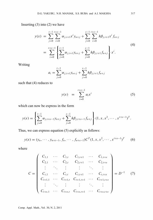
Inserting (3) into (2) we have
y(x) =t−1∑
j=0
t+s−1∑
i=0
α j,i+1xi yn+ j +s−1∑
j=0
t+s−1∑
i=0
hβ j,i+1xi fn+ j
=t+s−1∑
i=0
t−1∑
j=0
α j,i+1 yn+ j +s−1∑
j=0
hβ j,i+1 fn+ j
xi .
(4)
Writing
ai =t−1∑
j=0
α j,i+1 yn+ j +s−1∑
j=0
hβ j,i+1 fn+ j
such that (4) reduces to
y(x) =t+s−1∑
i=0
ai xi (5)
which can now be express in the form
y(x) =
t−1∑
j=0
α j,t+s−1 yn+ j +s−1∑
j=0
hβ j,t+s−1 fn+ j
(1, x, x2, ∙ ∙ ∙ , xt+s−1)T .
Thus, we can express equation (5) explicitly as follows:
y(x) = (yn, ∙ ∙ ∙ , yn+t−1, fn, ∙ ∙ ∙ , fn+s−1)CT (1, x, x2, ∙ ∙ ∙ , xt+s−1)T (6)
where
C =
C1,1 ∙ ∙ ∙ C1,t C1,t+1 ∙ ∙ ∙ C1,t+s
C2,1 ∙ ∙ ∙ C2,t C2,t+1 ∙ ∙ ∙ C2,t+s...
. . ....
.... . .
...
Ct,1 ∙ ∙ ∙ Ct,t Ct,t+1 ∙ ∙ ∙ Ct,t+s
Ct+1,1 ∙ ∙ ∙ Ct+1,t Ct+1,t+1 ∙ ∙ ∙ Ct+1,t+s...
. . ....
.... . .
...
Ct+s,1 ∙ ∙ ∙ Ct+s,t Ct+s,t+1 ∙ ∙ ∙ Ct+s,t+s
= D−1 (7)
Comp. Appl. Math., Vol. 30, N. 2, 2011
“main” — 2011/7/7 — 17:10 — page 318 — #4
318 UNIFORMLY ACCURATE ORDER L-R-K COLLOCATION METHODS
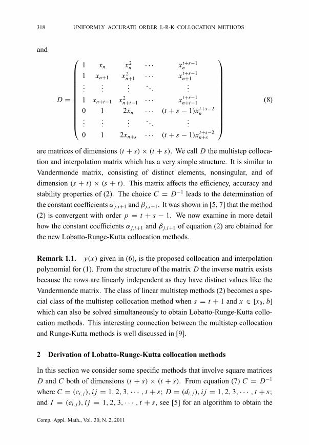
and
D =
1 xn x2n ∙ ∙ ∙ xt+s−1
n
1 xn+1 x2n+1 ∙ ∙ ∙ xt+s−1
n+1...
......
. . ....
1 xn+t−1 x2n+t−1 ∙ ∙ ∙ xt+s−1
n+t−1
0 1 2xn ∙ ∙ ∙ (t + s − 1)xt+s−2n
......
.... . .
...
0 1 2xn+s ∙ ∙ ∙ (t + s − 1)xt+s−2n+s
(8)
are matrices of dimensions (t + s) × (t + s). We call D the multistep colloca-
tion and interpolation matrix which has a very simple structure. It is similar to
Vandermonde matrix, consisting of distinct elements, nonsingular, and of
dimension (s + t) × (s + t). This matrix affects the efficiency, accuracy and
stability properties of (2). The choice C = D−1 leads to the determination of
the constant coefficients α j,i+1 and β j,i+1. It was shown in [5, 7] that the method
(2) is convergent with order p = t + s − 1. We now examine in more detail
how the constant coefficients α j,i+1 and β j,i+1 of equation (2) are obtained for
the new Lobatto-Runge-Kutta collocation methods.
Remark 1.1. y(x) given in (6), is the proposed collocation and interpolation
polynomial for (1). From the structure of the matrix D the inverse matrix exists
because the rows are linearly independent as they have distinct values like the
Vandermonde matrix. The class of linear multistep methods (2) becomes a spe-
cial class of the multistep collocation method when s = t + 1 and x ∈ [x0, b]
which can also be solved simultaneously to obtain Lobatto-Runge-Kutta collo-
cation methods. This interesting connection between the multistep collocation
and Runge-Kutta methods is well discussed in [9].
2 Derivation of Lobatto-Runge-Kutta collocation methods
In this section we consider some specific methods that involve square matrices
D and C both of dimensions (t + s) × (t + s). From equation (7) C = D−1
where C = (ci, j ), i j = 1, 2, 3, ∙ ∙ ∙ , t + s; D = (di, j ), i j = 1, 2, 3, ∙ ∙ ∙ , t + s;
and I = (ei, j ), i j = 1, 2, 3, ∙ ∙ ∙ , t + s, see [5] for an algorithm to obtain the
Comp. Appl. Math., Vol. 30, N. 2, 2011

“main” — 2011/7/7 — 17:10 — page 319 — #5
D.G. YAKUBU, N.H. MANJAK, S.S. BUBA and A.I. MAKSHA 319
elements of the matrices C , D and I . We shall derive multistep collocation
method as continuous single finite difference formula of non-uniform order six
based on Lobatto points see [8]. For s = 4, t = 1 and 2 = (x −xn) convergence
throughout the interval [x0, b], the matrix D of equation (8) takes the form:
D =
1 xn x2n x3
n x4n
0 1 2xn 3x2n 4x3
n
0 1 2xn+1 3x2n+1 4x3
n+1
0 1 2xn+u 3x2n+u 4x3
n+u
0 1 2xn+v 3x2n+v 4x3
n+v
(9)
where u and v are zeros of Lm(x) = 0, Lobatto polynomial [8] of degree m
which after certain transformation, we obtain
x0 = xn+u, u =
(1
2−
√5
10
)
, x1 = xn+v, v =
(1
2+
√5
10
)
(10)
which are valid in the interval [x0, b]. Inverting the matrix D in equation (9)
once, using computer algebra, for example, Maple or Matlab software package
we obtain the continuous scheme as:
y(2+xn
)= α0(x)yn +
[β0(x) fn +β1(x) fn+u +β2(x) fn+v +β3(x) fn+1
], (11)
where
α0(x) = −1
β0(x) =[−324 + 4(v + u + 1)h23 − 6(vu + v + u)h222 + 12vuh32
12vuh3
]
β1(x) =[−324 + 4(v + 1)h23 − 6vh222
12u(v − u)(u − 1)h3
]
β2(x) =[
324 − 4(u + 1)h23 + 6uh222
12v(v − u)(v − 1)h3
]
β3(x) =[
324 − 4(v + u)h23 + 6vuh222
12(v − 1)(u − 1)h3
].
Comp. Appl. Math., Vol. 30, N. 2, 2011

“main” — 2011/7/7 — 17:10 — page 320 — #6
320 UNIFORMLY ACCURATE ORDER L-R-K COLLOCATION METHODS
We evaluate y(x) in (11) at the following point x = xn+1, we recovered the
well known Lobatto IIIA with s = 4 and order p = 6, see [1] page 210, where
D′i s(i = 5, 7) are the error constants.
yn+1 = yn +h
12
[fn + 5 fn+u + 5 fn+v + fn+1
]
order p = 6, D7 = −6.613 × 10⁻⁷
yn+u = yn +h
120
[(11 +
√5) fn + (25 −
√5) fn+u
+(25 − 13√
5) fn+v + (−1 +√
5) fn+1]
order p = 4, D5 = −7.45 × 10⁻⁵
yn+v = yn +h
120
[(11 −
√5) fn + (25 + 13
√5) fn+u
+(25 +√
5) fn+v + (−1 −√
5) fn+1]
order p = 4, D5 = 7.45 × 10⁻⁵.
We converted the block hybrid scheme above to Lobatto-Runge-Kutta collo-
cation method, written as:
yn = yn−1 + h(
1
12
)F1 + h
(5
12
)F2 + h
(5
12
)F3 + h
(1
12
)F4 (12)
The stage values at the nth step are computed as:
Y1 = yn−1
Y2 = yn−1 + h
(11
120+
√5
120
)
F1 + h
(5
24−
√5
120
)
F2 + h
(5
24−
13√
5
120
)
F3 + h
(−1
120+
√5
120
)
F4
Y3 = yn−1 + h
(11
120−
√5
120
)
F1 + h
(5
24+
13√
5
120
)
F2 + h
(5
24+
√5
120
)
F3 + h
(
−1
120−
√5
120
)
F4
Y4 = yn−1 + h(
1
12
)F1 + h
(5
12
)F2 + h
(5
12
)F3 + h
(1
12
)F4
Comp. Appl. Math., Vol. 30, N. 2, 2011
“main” — 2011/7/7 — 17:10 — page 321 — #7
D.G. YAKUBU, N.H. MANJAK, S.S. BUBA and A.I. MAKSHA 321
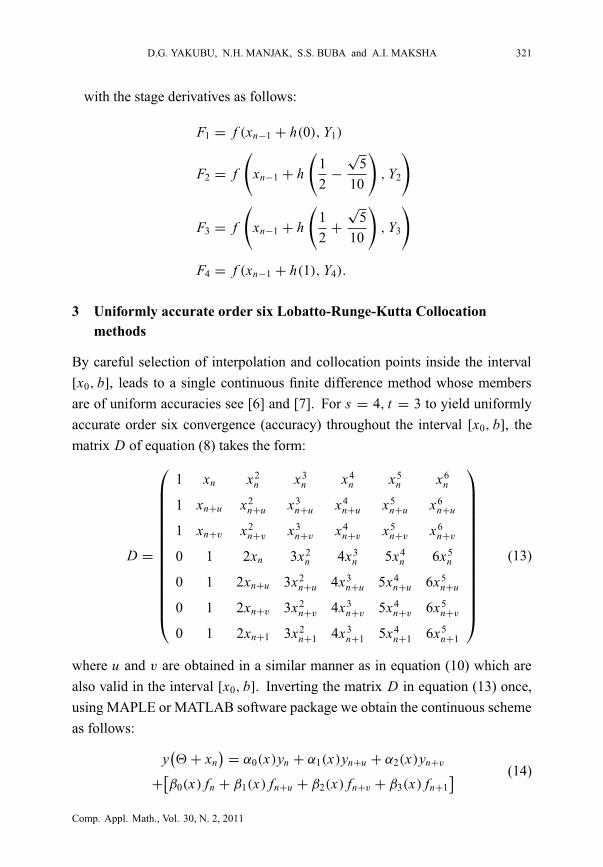
with the stage derivatives as follows:
F1 = f (xn−1 + h(0), Y1)
F2 = f
(
xn−1 + h
(1
2−
√5
10
)
, Y2
)
F3 = f
(
xn−1 + h
(1
2+
√5
10
)
, Y3
)
F4 = f (xn−1 + h(1), Y4).
3 Uniformly accurate order six Lobatto-Runge-Kutta Collocationmethods
By careful selection of interpolation and collocation points inside the interval
[x0, b], leads to a single continuous finite difference method whose members
are of uniform accuracies see [6] and [7]. For s = 4, t = 3 to yield uniformly
accurate order six convergence (accuracy) throughout the interval [x0, b], the
matrix D of equation (8) takes the form:
D =
1 xn x2n x3
n x4n x5
n x6n
1 xn+u x2n+u x3
n+u x4n+u x5
n+u x6n+u
1 xn+v x2n+v x3
n+v x4n+v x5
n+v x6n+v
0 1 2xn 3x2n 4x3
n 5x4n 6x5
n
0 1 2xn+u 3x2n+u 4x3
n+u 5x4n+u 6x5
n+u
0 1 2xn+v 3x2n+v 4x3
n+v 5x4n+v 6x5
n+v
0 1 2xn+1 3x2n+1 4x3
n+1 5x4n+1 6x5
n+1
(13)
where u and v are obtained in a similar manner as in equation (10) which are
also valid in the interval [x0, b]. Inverting the matrix D in equation (13) once,
using MAPLE or MATLAB software package we obtain the continuous scheme
as follows:
y(2 + xn
)= α0(x)yn + α1(x)yn+u + α2(x)yn+v
+[β0(x) fn + β1(x) fn+u + β2(x) fn+v + β3(x) fn+1
] (14)
Comp. Appl. Math., Vol. 30, N. 2, 2011
“main” — 2011/7/7 — 17:10 — page 322 — #8
322 UNIFORMLY ACCURATE ORDER L-R-K COLLOCATION METHODS
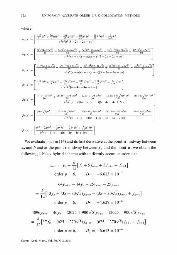
where
α0(x) =
[ −125 26 + 36
5 h25 − 19825 h224 + 96
25 h323 − 1825 h422 + 6
625 h6
u3v3h6[3 − 2v − 2u + vu]
]
α1(x) =
26(24−12
√5)
10 − 6h25(50−26√
5)50 + 3h224(82−46
√5)
50 − 2h323(36−24√
5)50 + 3h422(2−2
√5)
50
u3h6(v − u)(v − u)(u − v)[3 − 2v − 2u + vu]
α2(x) =
−26(24+12
√5)
10 + 6h25(50+26√
5)50 − 3h224(82+46
√5)
50 + 2h323(36+24√
5)50 − 3h422(2+2
√5)
50
v3h6(v − u)(v − u)(u − v)[3 − 2v − 2u + vu]
β0(x) =
[ −115 26 + 34
5 h25 − 19725 h224 + 106
25 h323 − 131125 h422 + 12
125 h52
u2v2h5[6 − 4v − 4u + 2vu]
]
β1(x) =
−(19+
√5)26
10 + 2(125+11√
5)h25
50 − (229+31√
5)h224
50 + 2(215+41√
5)h323
250 − (55+13√
5)h422
250
u2h5(v − u)(u − v)(u − 1)[6 − 4v − 4u + 2vu]
β2(x) =
(19−
√5)26
10 − 2(125−11√
5)h25
50 + (229−31√
5)h224
50 − 2(215−41√
5)h323
250 + (55−13√
5)h422
250
v2h5(v − u)(v − v)(v − 1)[6 − 4v − 4u + 2vu]
β3(x) =
[26 − 2h25 + 7
5 h224 − 25 h323 + 1
25 h422
h5(v − 1)(u − 1)[6 − 4v − 4u + 2vu]
]
.
We evaluate y(x) in (14) and its first derivative at the point w midway between
x0 and b and at the point r midway between xn and the point w, we obtain the
following 4-block hybrid scheme with uniformly accurate order six:
yn+1 = yn +h
12
[fn + 5 fn+u + 5 fn+v + fn+1
]
order p = 6, D7 = −6.613 × 10⁻⁷
64yn+w − 14yn − 25yn+u − 25yn+v
=h
12
[13 fn + (35 + 30
√5) fn+u + (35 − 30
√5) fn+v + fn+1
]
order p = 6, D7 = −4.629 × 10⁻⁶
4096yn+r − 46yn − (2025 + 900√
5)yn+u − (2025 − 900√
5)yn+v
=h
12
[37 fn − (625 + 270
√5) fn+u − (625 − 270
√5) fn+v + fn+1
]
order p = 6, D7 = −6.613 × 10⁻⁶
Comp. Appl. Math., Vol. 30, N. 2, 2011
“main” — 2011/7/7 — 17:10 — page 323 — #9
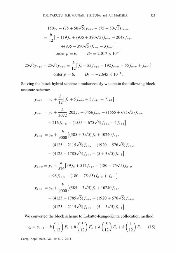
D.G. YAKUBU, N.H. MANJAK, S.S. BUBA and A.I. MAKSHA 323
150yn − (75 + 50√
5)yn+u − (75 − 50√
5)yn+v
=h
12
[− 119 fn + (935 + 390
√5) fn+u − 2048 fn+r
+(935 − 390√
5) fn+v − 3 fn+1]
order p = 6, D7 = 2.017 × 10⁻⁵
25√
5yn+u − 25√
5yn+v =h
12
[fn − 55 fn+u − 192 fn+w − 55 fn+v + fn+1
]
order p = 6, D7 = −2.645 × 10⁻⁶.
Solving the block hybrid scheme simultaneously we obtain the following block
accurate scheme:
yn+1 = yn +h
12
[fn + 5 fn+u + 5 fn+v + fn+1
]
yn+r = yn +h
3072
[202 fn + 3456 fn+r − (1555 + 675
√5) fn+u
+ 216 fn+w − (1555 − 675√
5) fn+v + 4 fn+1]
yn+u = yn +h
9000
[(585 + 3
√5) fn + 10240 fn+r
− (4125 + 2115√
5) fn+u + (1920 − 576√
5) fn+w
− (4125 − 1785√
5) fn+v + (5 + 3√
5) fn+1]
yn+w = yn +h
576
[39 fn + 512 fn+r − (180 + 75
√5) fn+u
+ 96 fn+w − (180 − 75√
5) fn+v + fn+1]
yn+v = yn +h
9000
[(585 − 3
√5) fn + 10240 fn+r
− (4125 + 1785√
5) fn+u + (1920 + 576√
5) fn+w
− (4125 − 2115√
5) fn+v + (5 − 3√
5) fn+1].
We converted the block scheme to Lobatto-Runge-Kutta collocation method:
yn = yn−1 + h(
1
12
)F1 + h
(5
12
)F3 + h
(5
12
)F5 + h
(1
12
)F6 (15)
Comp. Appl. Math., Vol. 30, N. 2, 2011
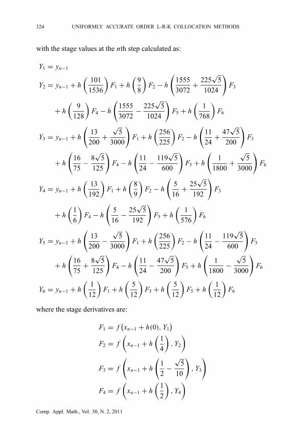
“main” — 2011/7/7 — 17:10 — page 324 — #10
324 UNIFORMLY ACCURATE ORDER L-R-K COLLOCATION METHODS
with the stage values at the nth step calculated as:
Y1 = yn−1
Y2 = yn−1 + h(
101
1536
)F1 + h
(9
8
)F2 − h
(1555
3072+
225√
5
1024
)
F3
+ h(
9
128
)F4 − h
(1555
3072−
225√
5
1024
)
F5 + h(
1
768
)F6
Y3 = yn−1 + h
(13
200+
√5
3000
)
F1 + h(
256
225
)F2 − h
(11
24+
47√
5
200
)
F3
+ h
(16
75−
8√
5
125
)
F4 − h
(11
24−
119√
5
600
)
F5 + h
(1
1800+
√5
3000
)
F6
Y4 = yn−1 + h(
13
192
)F1 + h
(8
9
)F2 − h
(5
16+
25√
5
192
)
F3
+ h(
1
6
)F4 − h
(5
16−
25√
5
192
)
F5 + h(
1
576
)F6
Y5 = yn−1 + h
(13
200−
√5
3000
)
F1 + h(
256
225
)F2 − h
(11
24−
119√
5
600
)
F3
+ h
(16
75+
8√
5
125
)
F4 − h
(11
24−
47√
5
200
)
F5 + h
(1
1800−
√5
3000
)
F6
Y6 = yn−1 + h(
1
12
)F1 + h
(5
12
)F3 + h
(5
12
)F5 + h
(1
12
)F6
where the stage derivatives are:
F1 = f(xn−1 + h(0), Y1
)
F2 = f(
xn−1 + h(
1
4
), Y2
)
F3 = f
(
xn−1 + h
(1
2−
√5
10
)
, Y3
)
F4 = f(
xn−1 + h(
1
2
), Y4
)
Comp. Appl. Math., Vol. 30, N. 2, 2011
“main” — 2011/7/7 — 17:10 — page 325 — #11
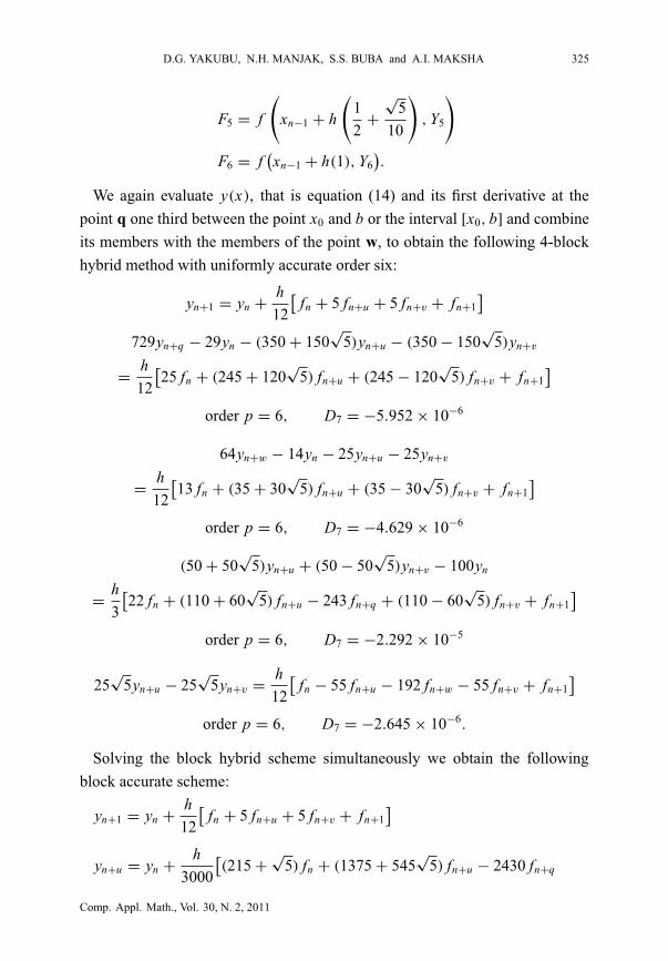
D.G. YAKUBU, N.H. MANJAK, S.S. BUBA and A.I. MAKSHA 325
F5 = f
(
xn−1 + h
(1
2+
√5
10
)
, Y5
)
F6 = f(xn−1 + h(1), Y6
).
We again evaluate y(x), that is equation (14) and its first derivative at the
point q one third between the point x0 and b or the interval [x0, b] and combine
its members with the members of the point w, to obtain the following 4-block
hybrid method with uniformly accurate order six:
yn+1 = yn +h
12
[fn + 5 fn+u + 5 fn+v + fn+1
]
729yn+q − 29yn − (350 + 150√
5)yn+u − (350 − 150√
5)yn+v
=h
12
[25 fn + (245 + 120
√5) fn+u + (245 − 120
√5) fn+v + fn+1
]
order p = 6, D7 = −5.952 × 10⁻⁶
64yn+w − 14yn − 25yn+u − 25yn+v
=h
12
[13 fn + (35 + 30
√5) fn+u + (35 − 30
√5) fn+v + fn+1
]
order p = 6, D7 = −4.629 × 10⁻⁶
(50 + 50√
5)yn+u + (50 − 50√
5)yn+v − 100yn
=h
3
[22 fn + (110 + 60
√5) fn+u − 243 fn+q + (110 − 60
√5) fn+v + fn+1
]
order p = 6, D7 = −2.292 × 10⁻⁵
25√
5yn+u − 25√
5yn+v =h
12
[fn − 55 fn+u − 192 fn+w − 55 fn+v + fn+1
]
order p = 6, D7 = −2.645 × 10⁻⁶.
Solving the block hybrid scheme simultaneously we obtain the following
block accurate scheme:
yn+1 = yn +h
12
[fn + 5 fn+u + 5 fn+v + fn+1
]
yn+u = yn +h
3000
[(215 +
√5) fn + (1375 + 545
√5) fn+u − 2430 fn+q
Comp. Appl. Math., Vol. 30, N. 2, 2011
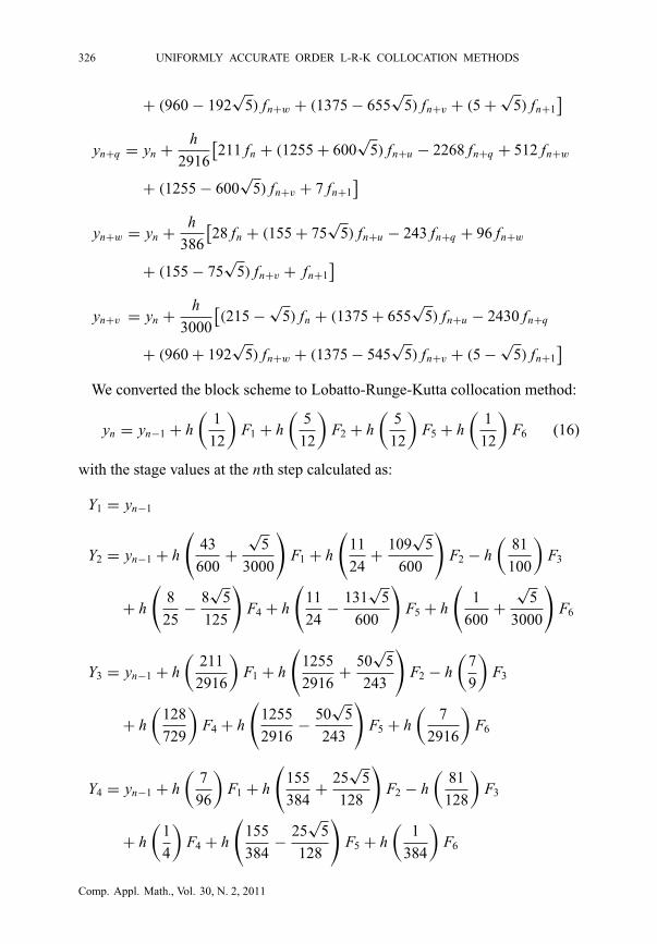
“main” — 2011/7/7 — 17:10 — page 326 — #12
326 UNIFORMLY ACCURATE ORDER L-R-K COLLOCATION METHODS
+ (960 − 192√
5) fn+w + (1375 − 655√
5) fn+v + (5 +√
5) fn+1]
yn+q = yn +h
2916
[211 fn + (1255 + 600
√5) fn+u − 2268 fn+q + 512 fn+w
+ (1255 − 600√
5) fn+v + 7 fn+1]
yn+w = yn +h
386
[28 fn + (155 + 75
√5) fn+u − 243 fn+q + 96 fn+w
+ (155 − 75√
5) fn+v + fn+1]
yn+v = yn +h
3000
[(215 −
√5) fn + (1375 + 655
√5) fn+u − 2430 fn+q
+ (960 + 192√
5) fn+w + (1375 − 545√
5) fn+v + (5 −√
5) fn+1]
We converted the block scheme to Lobatto-Runge-Kutta collocation method:
yn = yn−1 + h(
1
12
)F1 + h
(5
12
)F2 + h
(5
12
)F5 + h
(1
12
)F6 (16)
with the stage values at the nth step calculated as:
Y1 = yn−1
Y2 = yn−1 + h
(43
600+
√5
3000
)
F1 + h
(11
24+
109√
5
600
)
F2 − h(
81
100
)F3
+ h
(8
25−
8√
5
125
)
F4 + h
(11
24−
131√
5
600
)
F5 + h
(1
600+
√5
3000
)
F6
Y3 = yn−1 + h(
211
2916
)F1 + h
(1255
2916+
50√
5
243
)
F2 − h(
7
9
)F3
+ h(
128
729
)F4 + h
(1255
2916−
50√
5
243
)
F5 + h(
7
2916
)F6
Y4 = yn−1 + h(
7
96
)F1 + h
(155
384+
25√
5
128
)
F2 − h(
81
128
)F3
+ h(
1
4
)F4 + h
(155
384−
25√
5
128
)
F5 + h(
1
384
)F6
Comp. Appl. Math., Vol. 30, N. 2, 2011
“main” — 2011/7/7 — 17:10 — page 327 — #13
D.G. YAKUBU, N.H. MANJAK, S.S. BUBA and A.I. MAKSHA 327
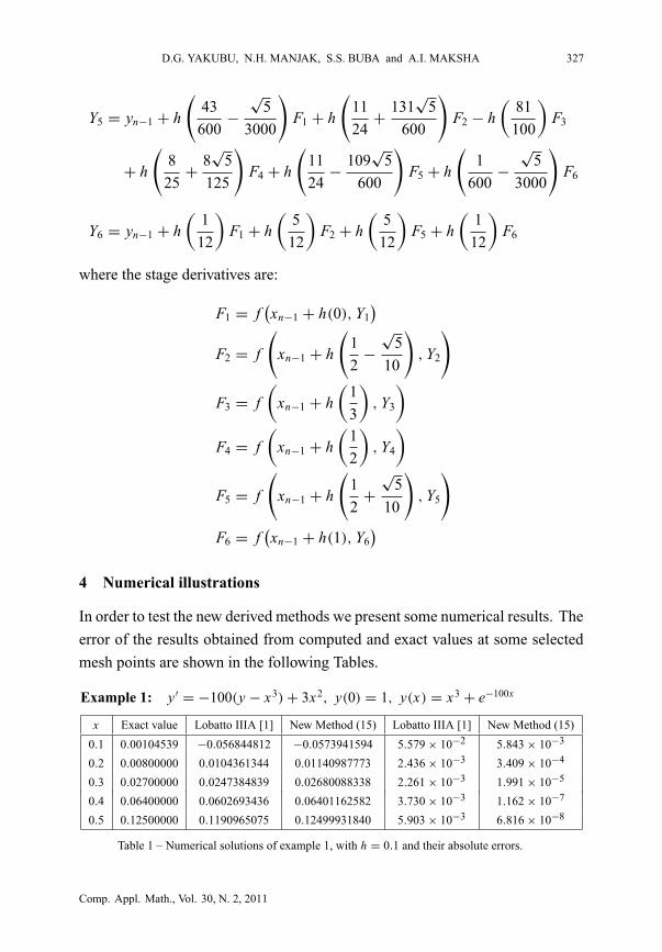
Y5 = yn−1 + h
(43
600−
√5
3000
)
F1 + h
(11
24+
131√
5
600
)
F2 − h(
81
100
)F3
+ h
(8
25+
8√
5
125
)
F4 + h
(11
24−
109√
5
600
)
F5 + h
(1
600−
√5
3000
)
F6
Y6 = yn−1 + h(
1
12
)F1 + h
(5
12
)F2 + h
(5
12
)F5 + h
(1
12
)F6
where the stage derivatives are:
F1 = f(xn−1 + h(0), Y1
)
F2 = f
(
xn−1 + h
(1
2−
√5
10
)
, Y2
)
F3 = f(
xn−1 + h(
1
3
), Y3
)
F4 = f(
xn−1 + h(
1
2
), Y4
)
F5 = f
(
xn−1 + h
(1
2+
√5
10
)
, Y5
)
F6 = f(xn−1 + h(1), Y6
)
4 Numerical illustrations
In order to test the new derived methods we present some numerical results. The
error of the results obtained from computed and exact values at some selected
mesh points are shown in the following Tables.
′ = − ( − ) + , ( ) = , ( ) = + −
. . − . − . . × − . × −
. . . . . × − . × −
. . . . . × − . × −
. . . . . × − . × −
. . . . . × − . × −
= .
Comp. Appl. Math., Vol. 30, N. 2, 2011
“main” — 2011/7/7 — 17:10 — page 328 — #14
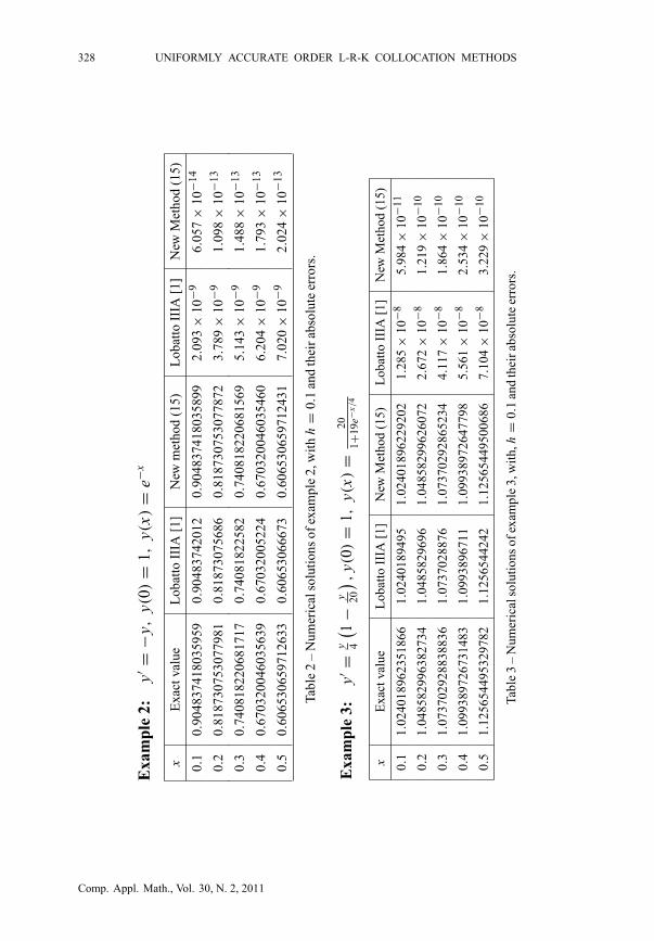
328 UNIFORMLY ACCURATE ORDER L-R-K COLLOCATION METHODS
′=
−,
()=
,(
)=
−
..
..
.×
−.
×−
..
..
.×
−.
×−
..
..
.×
−.
×−
..
..
.×
−.
×−
..
..
.×
−.
×−
=.
′=
(−
),
()=
,(
)=
+−
/
..
..
.×
−.
×−
..
..
.×
−.
×−
..
..
.×
−.
×−
..
..
.×
−.
×−
..
..
.×
−.
×−
=.
Comp. Appl. Math., Vol. 30, N. 2, 2011
“main” — 2011/7/7 — 17:10 — page 329 — #15
D.G. YAKUBU, N.H. MANJAK, S.S. BUBA and A.I. MAKSHA 329
5 Conclusions
Consequently the numerical results of Tables 1, 2 and 3 revealed the novelty
of the uniformly accurate order six methods which in fact give results closer to
the exact solutions at the expense of very low computational cost. Moreover,
as the first row of the matrix A consists of zeros, the first stage of each method
coincides with the initial value. And due to the requirement of stiff accuracy,
the last stage also coincides with the expression for the final point, which implies
that no further function evaluation is necessary to obtain yn+1 in each of the
method, see [3].
Acknowledgement. The first author wishes to express his sincere thanks and
appreciation to the referee for his/her thorough and very fair comments.
REFERENCES
[1] J.C. Butcher, Numerical Methods for Ordinary Differential Equations.
John Wiley (2003).
[2] J.C. Butcher, General linear methods. Compt. Math. Applic., 31(4-5) (1996),
105–112.
[3] J.C. Butcher and D.J.L. Chen, A new type of Singly-implicit Runge-Kutta
method. Applied Numer. Math., 34 (2000), 179–188.
[4] I. Lie and S.P. Nørsett, Super-Convergence for multistep collocation.
Math. Comp., 52 (1989), 65–80.
[5] P. Onumanyi, D.O. Awoyemi, S.N. Jatau and U.W. Sirisena, New linear
multistep methods with continuous coefficients for first order initial value
problems. Journal of the Nigerian Mathematical Society, 13 (1994), 37–51.
[6] D. Sarafyan, New algorithms for continuous approximate solution for
ordinary differential equations and the upgrading of the order of the pro-
cesses. Comp. Math. Applic., 20(1) (1990), 276–278.
[7] U.W. Sirisena, P. Onumanyi and D.G. Yakubu, Towards uniformly accurate
continuous Finite Difference Approximation of ODEs. B. Journal of Pure
and Applied Sciences, 1 (2001), 1–5.
Comp. Appl. Math., Vol. 30, N. 2, 2011
“main” — 2011/7/7 — 17:10 — page 330 — #16
330 UNIFORMLY ACCURATE ORDER L-R-K COLLOCATION METHODS
[8] J. Villadsen and M.L. Michelsen, Solution of Differential Equations models
by polynomial approximations. Prentice-Hall Inc Eaglewood Cliffs, New
Jersey (1987), 112.
[9] D.G. Yakubu, Some new implicit Runge-Kutta methods from collocation
for initial value problem in ordinary differential equations. Ph.D. Thesis
Abubakar Tafawa Balewa University, Bauchi, Nigeria (2003), 65–70.
Comp. Appl. Math., Vol. 30, N. 2, 2011