A EUCLIDEAN FORMULATION OF INTERIOR ORIENTATION COSTRAINTS ...portal.survey.ntua.gr/main/labs/photo/staff/gkarras/Karras_isprs... · A EUCLIDEAN FORMULATION OF INTERIOR ORIENTATION

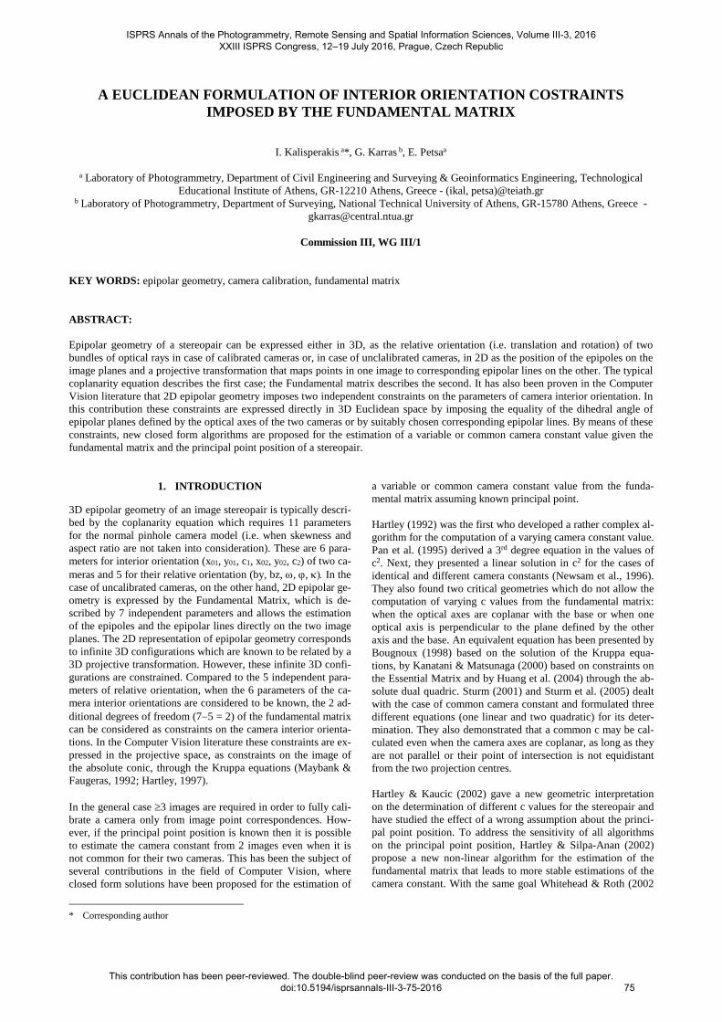
A EUCLIDEAN FORMULATION OF INTERIOR ORIENTATION COSTRAINTS IMPOSED BY THE FUNDAMENTAL MATRIX

I. Kalisperakis a*, G. Karras b, E. Petsaa

a Laboratory of Photogrammetry, Department of Civil Engineering and Surveying & Geoinformatics Engineering, Technological

Educational Institute of Athens, GR-12210 Athens, Greece - (ikal, petsa)@teiath.gr b Laboratory of Photogrammetry, Department of Surveying, National Technical University of Athens, GR-15780 Athens, Greece -

[email protected]

Commission III, WG III/1

KEY WORDS: epipolar geometry, camera calibration, fundamental matrix ABSTRACT: Epipolar geometry of a stereopair can be expressed either in 3D, as the relative orientation (i.e. translation and rotation) of two bundles of optical rays in case of calibrated cameras or, in case of unclalibrated cameras, in 2D as the position of the epipoles on the image planes and a projective transformation that maps points in one image to corresponding epipolar lines on the other. The typical coplanarity equation describes the first case; the Fundamental matrix describes the second. It has also been proven in the Computer Vision literature that 2D epipolar geometry imposes two independent constraints on the parameters of camera interior orientation. In this contribution these constraints are expressed directly in 3D Euclidean space by imposing the equality of the dihedral angle of epipolar planes defined by the optical axes of the two cameras or by suitably chosen corresponding epipolar lines. By means of these constraints, new closed form algorithms are proposed for the estimation of a variable or common camera constant value given the fundamental matrix and the principal point position of a stereopair.

* Corresponding author

1. INTRODUCTION

3D epipolar geometry of an image stereopair is typically descri-bed by the coplanarity equation which requires 11 parameters for the normal pinhole camera model (i.e. when skewness and aspect ratio are not taken into consideration). These are 6 para-meters for interior orientation (x01, y01, c1, x02, y02, c2) of two ca-meras and 5 for their relative orientation (by, bz, ω, ϕ, κ). In the case of uncalibrated cameras, on the other hand, 2D epipolar ge-ometry is expressed by the Fundamental Matrix, which is de-scribed by 7 independent parameters and allows the estimation of the epipoles and the epipolar lines directly on the two image planes. The 2D representation of epipolar geometry corresponds to infinite 3D configurations which are known to be related by a 3D projective transformation. However, these infinite 3D confi-gurations are constrained. Compared to the 5 independent para-meters of relative orientation, when the 6 parameters of the ca-mera interior orientations are considered to be known, the 2 ad-ditional degrees of freedom (7−5 = 2) of the fundamental matrix can be considered as constraints on the camera interior orienta-tions. In the Computer Vision literature these constraints are ex-pressed in the projective space, as constraints on the image of the absolute conic, through the Kruppa equations (Maybank & Faugeras, 1992; Hartley, 1997). In the general case ≥3 images are required in order to fully cali-brate a camera only from image point correspondences. How-ever, if the principal point position is known then it is possible to estimate the camera constant from 2 images even when it is not common for their two cameras. This has been the subject of several contributions in the field of Computer Vision, where closed form solutions have been proposed for the estimation of

a variable or common camera constant value from the funda-mental matrix assuming known principal point. Hartley (1992) was the first who developed a rather complex al-gorithm for the computation of a varying camera constant value. Pan et al. (1995) derived a 3rd degree equation in the values of c2. Next, they presented a linear solution in c2 for the cases of identical and different camera constants (Newsam et al., 1996). They also found two critical geometries which do not allow the computation of varying c values from the fundamental matrix: when the optical axes are coplanar with the base or when one optical axis is perpendicular to the plane defined by the other axis and the base. An equivalent equation has been presented by Bougnoux (1998) based on the solution of the Kruppa equa-tions, by Kanatani & Matsunaga (2000) based on constraints on the Essential Matrix and by Huang et al. (2004) through the ab-solute dual quadric. Sturm (2001) and Sturm et al. (2005) dealt with the case of common camera constant and formulated three different equations (one linear and two quadratic) for its deter-mination. They also demonstrated that a common c may be cal-culated even when the camera axes are coplanar, as long as they are not parallel or their point of intersection is not equidistant from the two projection centres. Hartley & Kaucic (2002) gave a new geometric interpretation on the determination of different c values for the stereopair and have studied the effect of a wrong assumption about the princi-pal point position. To address the sensitivity of all algorithms on the principal point position, Hartley & Silpa-Anan (2002) propose a new non-linear algorithm for the estimation of the fundamental matrix that leads to more stable estimations of the camera constant. With the same goal Whitehead & Roth (2002

ISPRS Annals of the Photogrammetry, Remote Sensing and Spatial Information Sciences, Volume III-3, 2016 XXIII ISPRS Congress, 12–19 July 2016, Prague, Czech Republic

This contribution has been peer-reviewed. The double-blind peer-review was conducted on the basis of the full paper. doi:10.5194/isprsannals-III-3-75-2016

75

and 2004) use the DHC (dynamic hill climbing) method, while Kanatani et al. (2006) compute a new fundamental matrix from fewer point correspondences. Stewénius et al. (2005) dealt first with the simultaneous estima-tion of relative orientation and a single camera constant value from 6 point correspondences through the theory of Gröbner ba-ses, and found the existence of 15, real and imaginary, solu-tions. A more straightforward solution was given by Li (2006) who proposed a 15th degree polynomial using the hidden vari-able method. Finally, Ronda & Valdés (2007) have examined the Kruppa equations in the case of a stereopair and, based on a projective geometry theorem of the French mathematician Pon-celet, propose a parameterization of all possible solutions for camera calibration. In this contribution the constraints that the fundamental matrix imposes on the interior orientation parameters are derived in 3D Euclidean space. The epipoles, the projection centers and the epipolar lines of the principal points allow the estimation, inde-pendently on each image plane, of the dihedral angle formed by the epipolar planes of the optical axes. The equality of the esti-mation of this angle from the two images imposes one geome-tric and algebraic constraint on the interior orientation parame-ters. A second independent constraint is derived in a similar way from the equality of the dihedral angle of the epipolar pla-nes that correspond to two suitably chosen epipolar lines. By means of these constraints four new closed form algorithms are developed for the computation of a common and variable came-ra constant from the fundamental matrix assuming known prin-cipal point.

2. INTERIOR ORIENTATION CONSTRAINTS

2.1 Dihedral angle of the epipolar planes defined by the optical axes of a stereopair

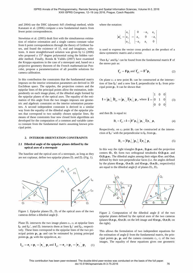
The baseline and the optical axes of a stereopair, as long as they are not coplanar, define two epipolar planes Π1 and Π2 (Fig. 1).

Figure 1. Epipolar planes Π1, Π2 of the optical axes of the two cameras define a dihedral angle β.

Plane Π1 intersects the two image planes ε1, ε2 at epipolar lines lp1 and lp1′, and Π2 intersects them at lines lp2′ and lp2, respecti-vely. These lines correspond to the epipolar lines of the two pri-ncipal points p1, p2 and can be estimated by joining principal points p1, p2 with the epipoles e1, e2:

[ ]p1 1 1 1 1l e p e p×

= × = and [ ]p2 2 2 2 2l e p e p×

= × = (1)

where the notation:

[ ]1 3 2

2 3 1

3 2 1

a 0 a a

a a 0 a

a a a 0×

×

− = = − −

a

is used to express the vector cross product as the product of a skew-symmetric matrix and a vector. Then lp1′ and lp2′ can be found from the fundamental matrix F of the stereo pair as:

p1 1l Fp′ = and Tp2 2l F p′ = (2)

On plane ε1 a new point Β1 can be constructed at the intersec-tion of line lp2′ and a new line l, perpendicular to lp1 from prin-cipal point p1. It can be shown that:

[ ] [ ] [ ]1 p1 1 1 1l p l p e p× × ×

= =ɶ ɶI I , where

1 0 0

0 1 0

0 0 0

=

ɶI (3)

and then Β1 is equal to:

[ ] [ ]T1 p2 2 1 1 1l l F p p e p

× ××

′= × = ɶIΒ (4)

Respectively, on ε2 point Β2 can be constructed at the interse-ction of lp1′ with the perpendicular to lp2 from p2.

[ ] [ ] [ ]2 1 2 2 2Fp p e p× × ×

= ɶIΒ (5)

In this way the right triangles Β1p1e1, Β2p2e2 and the projection centers O1, O2 form two orthogonal tetrahedra O1Β1p1e1 and O2Β2p2e2. The dihedral angles among their edges O1e1 and O2e2 defined by their non-perpendicular faces (i.e. the angles defined by the planes O1e1p1, O1e1Β1 and O2e2p2, O2e2Β2, respectively) are equal to the dihedral angle β of planes Π1, Π2.

Figure 2. Computation of the dihedral angle β of the two epipolar planes defined by the optical axes of the two cameras (planes O1e1p1, O1e1Β1 on the left image and O2e2p2, O2e2Β2 on the right).

This allows the formulation of two independent equations for the estimation of angle β from the fundamental matrix, the prin-cipal points p1, p2 and the camera constants c1, c2 of the two images. The equality of these equations gives one geometric



76

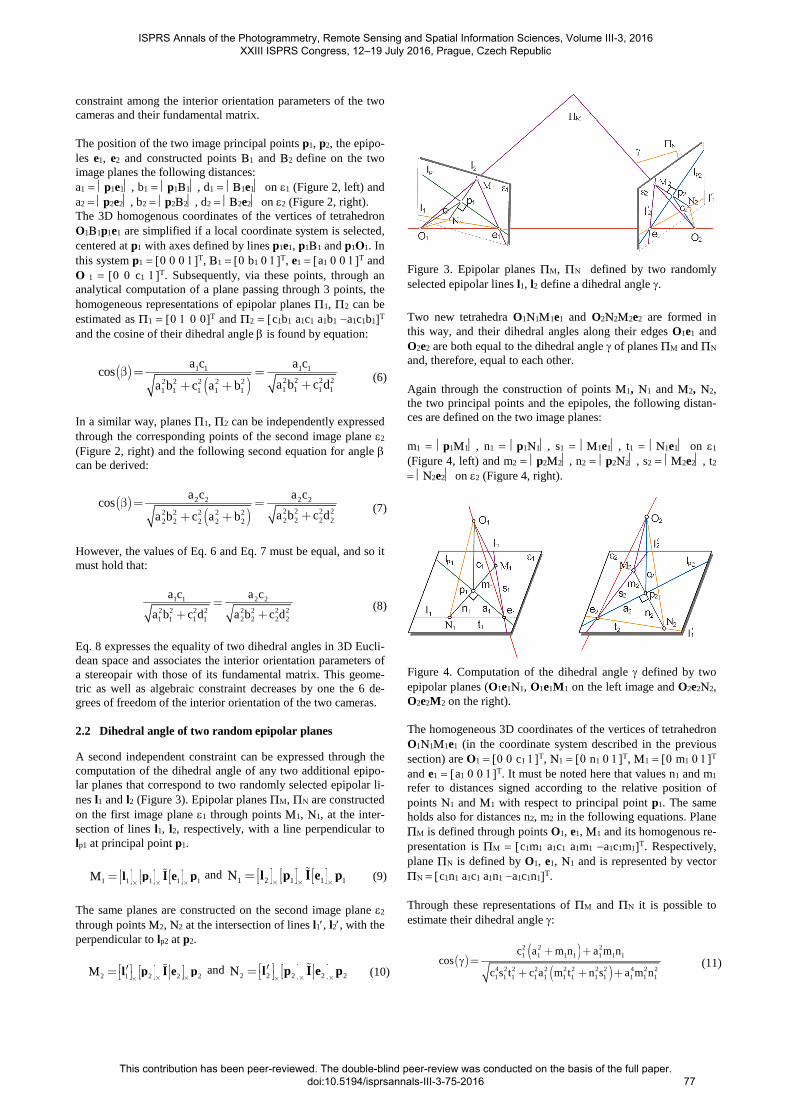
constraint among the interior orientation parameters of the two cameras and their fundamental matrix. The position of the two image principal points p1, p2, the epipo-les e1, e2 and constructed points Β1 and Β2 define on the two image planes the following distances: a1 = p1e1, b1 = p1Β1, d1 = Β1e1 on ε1 (Figure 2, left) and a2 = p2e2, b2 = p2Β2, d2 = Β2e2 on ε2 (Figure 2, right). The 3D homogenous coordinates of the vertices of tetrahedron O1Β1p1e1 are simplified if a local coordinate system is selected, centered at p1 with axes defined by lines p1e1, p1Β1 and p1Ο1. In this system p1 = [0 0 0 1]T, Β1 = [0 b1 0 1]T, e1 = [a1 0 0 1]T and Ο 1 = [0 0 c1 1]T. Subsequently, via these points, through an analytical computation of a plane passing through 3 points, the homogeneous representations of epipolar planes Π1, Π2 can be estimated as Π1 = [0 1 0 0]T and Π2 = [c1b1 a1c1 a1b1 −a1c1b1]T and the cosine of their dihedral angle β is found by equation:

( )( )

1 1 1 1

2 2 2 22 2 2 2 21 1 1 11 1 1 1 1

a c a ccos

a b c da b c a bβ = =

++ +

(6)

In a similar way, planes Π1, Π2 can be independently expressed through the corresponding points of the second image plane ε2 (Figure 2, right) and the following second equation for angle β can be derived:

( )( )

2 2 2 2

2 2 2 22 2 2 2 22 2 2 22 2 2 2 2

a c a ccos

a b c da b c a bβ = =

++ +

(7)

However, the values of Eq. 6 and Eq. 7 must be equal, and so it must hold that:

1 1 2 2

2 2 2 2 2 2 2 21 1 1 1 2 2 2 2

a c a c

a b c d a b c d=

+ +

(8)

Eq. 8 expresses the equality of two dihedral angles in 3D Eucli-dean space and associates the interior orientation parameters of a stereopair with those of its fundamental matrix. This geome-tric as well as algebraic constraint decreases by one the 6 de-grees of freedom of the interior orientation of the two cameras. 2.2 Dihedral angle of two random epipolar planes

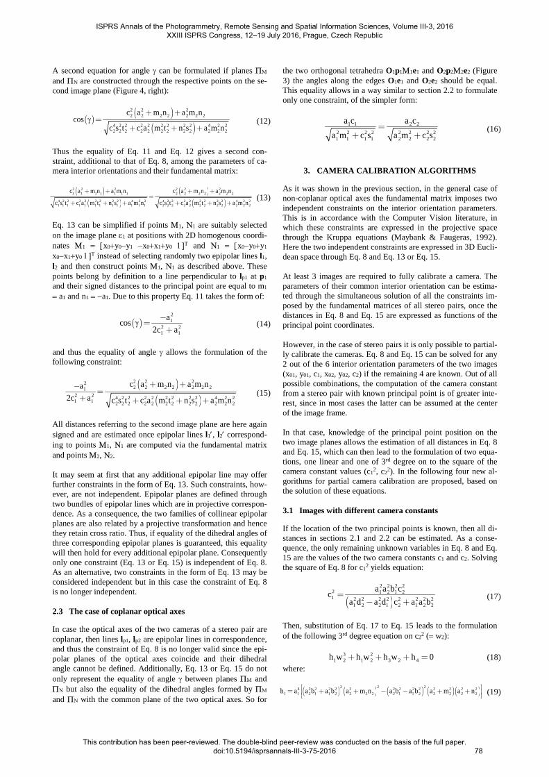
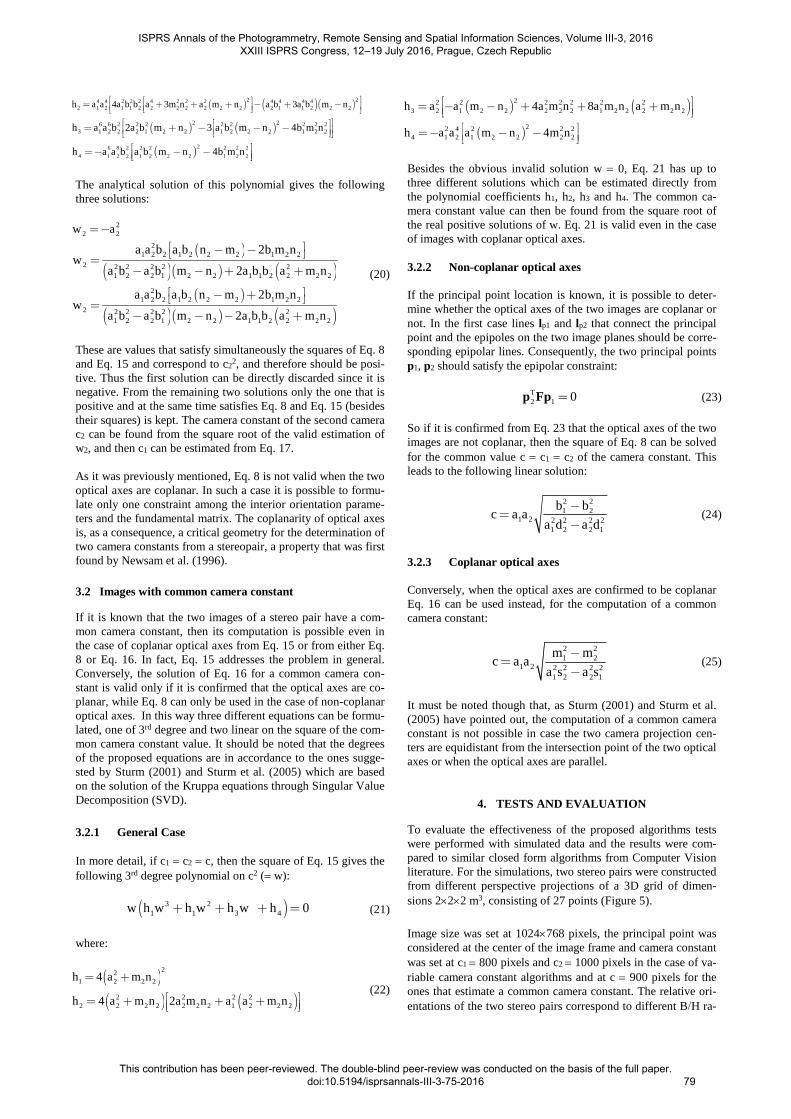
A second independent constraint can be expressed through the computation of the dihedral angle of any two additional epipo-lar planes that correspond to two randomly selected epipolar li-nes l1 and l2 (Figure 3). Epipolar planes ΠΜ, ΠΝ are constructed on the first image plane ε1 through points Μ1, Ν1, at the inter-section of lines l1, l2, respectively, with a line perpendicular to lp1 at principal point p1.

[ ] [ ] [ ]1 1 1 1 1l p e p× × ×

= ɶIΜ and [ ] [ ] [ ]1 2 1 1 1l p e p× × ×

= ɶIΝ (9)

The same planes are constructed on the second image plane ε2 through points Μ2, Ν2 at the intersection of lines l1′, l2′, with the perpendicular to lp2 at p2.

[ ] [ ]2 1 2 2 2l p e p× ××

′= ɶIΜ and [ ] [ ]2 2 2 2 2l p e p

× ×× ′=

ɶIΝ (10)

Figure 3. Epipolar planes ΠΜ, ΠΝ defined by two randomly selected epipolar lines l1, l2 define a dihedral angle γ. Two new tetrahedra O1Ν1Μ1e1 and O2Ν2Μ2e2 are formed in this way, and their dihedral angles along their edges O1e1 and O2e2 are both equal to the dihedral angle γ of planes ΠΜ and ΠΝ and, therefore, equal to each other. Again through the construction of points Μ1, Ν1 and Μ2, Ν2, the two principal points and the epipoles, the following distan-ces are defined on the two image planes: m1 = p1Μ1, n1 = p1Ν1, s1 = Μ1e1, t1 = Ν1e1 on ε1 (Figure 4, left) and m2 = p2Μ2, n2 = p2Ν2, s2 = Μ2e2, t2 = Ν2e2 on ε2 (Figure 4, right).

Figure 4. Computation of the dihedral angle γ defined by two epipolar planes (O1e1Ν1, O1e1M1 on the left image and O2e2Ν2, O2e2M2 on the right). The homogeneous 3D coordinates of the vertices of tetrahedron O1Ν1Μ1e1 (in the coordinate system described in the previous section) are Ο1 = [0 0 c1 1]T, Ν1 = [0 n1 0 1]T, Μ1 = [0 m1 0 1]T and e1 = [a1 0 0 1]T. It must be noted here that values n1 and m1 refer to distances signed according to the relative position of points Ν1 and Μ1 with respect to principal point p1. The same holds also for distances n2, m2 in the following equations. Plane ΠΜ is defined through points O1, e1, Μ1 and its homogenous re-presentation is ΠΜ = [c1m1 a1c1 a1m1 −a1c1m1]T. Respectively, plane ΠΝ is defined by O1, e1, Ν1 and is represented by vector ΠΝ = [c1n1 a1c1 a1n1 −a1c1n1]T. Through these representations of ΠΜ and ΠΝ it is possible to estimate their dihedral angle γ:

( )( )

( )

2 2 21 1 1 1 1 1 1

4 2 2 2 2 2 2 2 2 4 2 21 1 1 1 1 1 1 1 1 1 1 1

c a m n a m ncos

c s t c a m t n s a m nγ

+ +=

+ + +

(11)



77

A second equation for angle γ can be formulated if planes ΠΜ and ΠΝ are constructed through the respective points on the se-cond image plane (Figure 4, right):

( )( )

( )

2 2 22 2 2 2 2 2 2

4 2 2 2 2 2 2 2 2 4 2 22 2 2 2 2 2 2 2 2 2 2 2

c a m n a m ncos

c s t c a m t n s a m nγ

+ +=

+ + +

(12)

Thus the equality of Eq. 11 and Eq. 12 gives a second con-straint, additional to that of Eq. 8, among the parameters of ca-mera interior orientations and their fundamental matrix:

( )

( )

( )

( )

2 2 2 2 2 21 1 1 1 1 1 1 2 2 2 2 2 2 2

4 2 2 2 2 2 2 2 2 4 2 2 4 2 2 2 2 2 2 2 2 4 2 21 1 1 1 1 1 1 1 1 1 1 1 2 2 2 2 2 2 2 2 2 2 2 2

c a m n a m n c a m n a m n

c s t c a m t n s a m n c s t c a m t n s a m n

+ + + +=

+ + + + + +

(13)

Eq. 13 can be simplified if points Μ1, Ν1 are suitably selected on the image plane ε1 at positions with 2D homogenous coordi-nates Μ1 = [x0+y0−y1 −x0+x1+y0 1]T and Ν1 = [x0−y0+y1 x0−x1+y0 1]T instead of selecting randomly two epipolar lines l1, l2 and then construct points Μ1, Ν1 as described above. These points belong by definition to a line perpendicular to lp1 at p1 and their signed distances to the principal point are equal to m1 = a1 and n1 = −a1. Due to this property Eq. 11 takes the form of:

( )21

2 21 1

acos

2c aγ

−=

+ (14)

and thus the equality of angle γ allows the formulation of the following constraint:

( )

( )

2 2 222 2 2 2 2 2 21

2 2 4 2 2 2 2 2 2 2 2 4 2 21 1 2 2 2 2 2 2 2 2 2 2 2 2

c a m n a m na

2c a c s t c a m t n s a m n

+ +−=

+ + + +

(15)

All distances referring to the second image plane are here again signed and are estimated once epipolar lines l1′, l2′ correspond-ing to points Μ1, Ν1 are computed via the fundamental matrix and points Μ2, Ν2. It may seem at first that any additional epipolar line may offer further constraints in the form of Eq. 13. Such constraints, how-ever, are not independent. Epipolar planes are defined through two bundles of epipolar lines which are in projective correspon-dence. As a consequence, the two families of collinear epipolar planes are also related by a projective transformation and hence they retain cross ratio. Thus, if equality of the dihedral angles of three corresponding epipolar planes is guaranteed, this equality will then hold for every additional epipolar plane. Consequently only one constraint (Eq. 13 or Eq. 15) is independent of Eq. 8. As an alternative, two constraints in the form of Eq. 13 may be considered independent but in this case the constraint of Eq. 8 is no longer independent. 2.3 The case of coplanar optical axes

In case the optical axes of the two cameras of a stereo pair are coplanar, then lines lp1, lp2 are epipolar lines in correspondence, and thus the constraint of Eq. 8 is no longer valid since the epi-polar planes of the optical axes coincide and their dihedral angle cannot be defined. Additionally, Eq. 13 or Eq. 15 do not only represent the equality of angle γ between planes ΠΜ and ΠΝ but also the equality of the dihedral angles formed by ΠΜ and ΠΝ with the common plane of the two optical axes. So for

the two orthogonal tetrahedra O1p1Μ1e1 and O2p2Μ2e2 (Figure 3) the angles along the edges O1e1 and O2e2 should be equal. This equality allows in a way similar to section 2.2 to formulate only one constraint, of the simpler form:

1 1 2 2

2 2 2 2 2 2 2 21 1 1 1 2 2 2 2

a c a c

a m c s a m c s=

+ + (16)

3. CAMERA CALIBRATION ALGORITHMS

As it was shown in the previous section, in the general case of non-coplanar optical axes the fundamental matrix imposes two independent constraints on the interior orientation parameters. This is in accordance with the Computer Vision literature, in which these constraints are expressed in the projective space through the Kruppa equations (Maybank & Faugeras, 1992). Here the two independent constraints are expressed in 3D Eucli-dean space through Eq. 8 and Eq. 13 or Eq. 15. At least 3 images are required to fully calibrate a camera. The parameters of their common interior orientation can be estima-ted through the simultaneous solution of all the constraints im-posed by the fundamental matrices of all stereo pairs, once the distances in Eq. 8 and Eq. 15 are expressed as functions of the principal point coordinates. However, in the case of stereo pairs it is only possible to partial-ly calibrate the cameras. Eq. 8 and Eq. 15 can be solved for any 2 out of the 6 interior orientation parameters of the two images (x01, y01, c1, x02, y02, c2) if the remaining 4 are known. Out of all possible combinations, the computation of the camera constant from a stereo pair with known principal point is of greater inte-rest, since in most cases the latter can be assumed at the center of the image frame. In that case, knowledge of the principal point position on the two image planes allows the estimation of all distances in Eq. 8 and Eq. 15, which can then lead to the formulation of two equa-tions, one linear and one of 3rd degree on to the square of the camera constant values (c1

2, c22). In the following four new al-

gorithms for partial camera calibration are proposed, based on the solution of these equations. 3.1 Images with different camera constants

If the location of the two principal points is known, then all di-stances in sections 2.1 and 2.2 can be estimated. As a conse-quence, the only remaining unknown variables in Eq. 8 and Eq. 15 are the values of the two camera constants c1 and c2. Solving the square of Eq. 8 for c1

2 yields equation:

( )

2 2 2 22 1 2 1 21 2 2 2 2 2 2 2 2

1 2 2 1 2 1 2 2

a a b cc

a d a d c a a b=

− + (17)

Then, substitution of Eq. 17 to Eq. 15 leads to the formulation of the following 3rd degree equation on c2

2 (= w2):

3 21 2 1 2 3 2 4h w h w h w h 0+ + + = (18)

where:

( ) ( ) ( ) ( )( )2 2 24 2 2 2 2 2 2 2 2 2 2 2 2 2

1 1 2 1 1 2 2 2 2 2 1 1 2 2 2 2 2h a a b a b a m n a b a b a m a n = + + − − + +

(19)



78

( ) ( )( )2 24 4 2 2 2 4 2 2 2 4 4 4 4

2 1 2 1 1 2 2 2 2 2 2 2 2 1 1 2 2 2h a a 4a b b a 3m n a m n a b 3a b m n = + + + − + −

( ) ( )2 26 6 2 2 2 2 2 2 2 2

3 1 2 2 2 1 2 2 1 2 2 2 1 2 2h a a b 2a b m n 3 a b m n 4b m n = + − − −

( )26 8 2 2 2 2 2 2

4 1 2 2 1 2 2 2 1 2 2h a a b a b m n 4b m n=− − −

The analytical solution of this polynomial gives the following three solutions:

22 2w a=−

( )

( )( ) ( )

21 2 2 1 2 2 2 1 2 2

2 2 2 2 2 21 2 2 1 2 2 1 1 2 2 2 2

a a b a b n m 2b m nw

a b a b m n 2a b b a m n

− − =− − + +

( )

( )( ) ( )

21 2 2 1 2 2 2 1 2 2

2 2 2 2 2 21 2 2 1 2 2 1 1 2 2 2 2

a a b a b n m 2b m nw

a b a b m n 2a b b a m n

− + =− − − +

(20)

These are values that satisfy simultaneously the squares of Eq. 8 and Eq. 15 and correspond to c2

2, and therefore should be posi-tive. Thus the first solution can be directly discarded since it is negative. From the remaining two solutions only the one that is positive and at the same time satisfies Eq. 8 and Eq. 15 (besides their squares) is kept. The camera constant of the second camera c2 can be found from the square root of the valid estimation of w2, and then c1 can be estimated from Eq. 17. As it was previously mentioned, Eq. 8 is not valid when the two optical axes are coplanar. In such a case it is possible to formu-late only one constraint among the interior orientation parame-ters and the fundamental matrix. The coplanarity of optical axes is, as a consequence, a critical geometry for the determination of two camera constants from a stereopair, a property that was first found by Newsam et al. (1996).

3.2 Images with common camera constant

If it is known that the two images of a stereo pair have a com-mon camera constant, then its computation is possible even in the case of coplanar optical axes from Eq. 15 or from either Eq. 8 or Eq. 16. In fact, Eq. 15 addresses the problem in general. Conversely, the solution of Eq. 16 for a common camera con-stant is valid only if it is confirmed that the optical axes are co-planar, while Eq. 8 can only be used in the case of non-coplanar optical axes. In this way three different equations can be formu-lated, one of 3rd degree and two linear on the square of the com-mon camera constant value. It should be noted that the degrees of the proposed equations are in accordance to the ones sugge-sted by Sturm (2001) and Sturm et al. (2005) which are based on the solution of the Kruppa equations through Singular Value Decomposition (SVD).

3.2.1 General Case In more detail, if c1 = c2 = c, then the square of Eq. 15 gives the following 3rd degree polynomial on c2 (= w):

( )3 21 1 3 4w h w h w h w h 0+ + + = (21)

where:

( )22

1 2 2 2h 4 a m n= +

( ) ( )2 2 2 22 2 2 2 2 2 2 1 2 2 2h 4 a m n 2a m n a a m n = + + +

(22)

( ) ( )22 2 2 2 2 2 23 2 1 2 2 2 2 2 1 2 2 2 2 2h a a m n 4a m n 8a m n a m n = − − + + +

( )22 4 2 2 2

4 1 2 1 2 2 2 2h a a a m n 4m n =− − −

Besides the obvious invalid solution w = 0, Eq. 21 has up to three different solutions which can be estimated directly from the polynomial coefficients h1, h2, h3 and h4. The common ca-mera constant value can then be found from the square root of the real positive solutions of w. Eq. 21 is valid even in the case of images with coplanar optical axes. 3.2.2 Non-coplanar optical axes If the principal point location is known, it is possible to deter-mine whether the optical axes of the two images are coplanar or not. In the first case lines lp1 and lp2 that connect the principal point and the epipoles on the two image planes should be corre-sponding epipolar lines. Consequently, the two principal points p1, p2 should satisfy the epipolar constraint:

T2 1 0p Fp = (23)

So if it is confirmed from Eq. 23 that the optical axes of the two images are not coplanar, then the square of Eq. 8 can be solved for the common value c = c1 = c2 of the camera constant. This leads to the following linear solution:

2 21 2

1 2 2 2 2 21 2 2 1

b bc a a

a d a d

−=

− (24)

3.2.3 Coplanar optical axes Conversely, when the optical axes are confirmed to be coplanar Eq. 16 can be used instead, for the computation of a common camera constant:

2 21 2

1 2 2 2 2 21 2 2 1

m mc a a

a s a s

−=

− (25)

It must be noted though that, as Sturm (2001) and Sturm et al. (2005) have pointed out, the computation of a common camera constant is not possible in case the two camera projection cen-ters are equidistant from the intersection point of the two optical axes or when the optical axes are parallel.

4. TESTS AND EVALUATION

To evaluate the effectiveness of the proposed algorithms tests were performed with simulated data and the results were com-pared to similar closed form algorithms from Computer Vision literature. For the simulations, two stereo pairs were constructed from different perspective projections of a 3D grid of dimen-sions 2×2×2 m3, consisting of 27 points (Figure 5).

Image size was set at 1024×768 pixels, the principal point was considered at the center of the image frame and camera constant was set at c1 = 800 pixels and c2 = 1000 pixels in the case of va-riable camera constant algorithms and at c = 900 pixels for the ones that estimate a common camera constant. The relative ori-entations of the two stereo pairs correspond to different B/H ra-



79

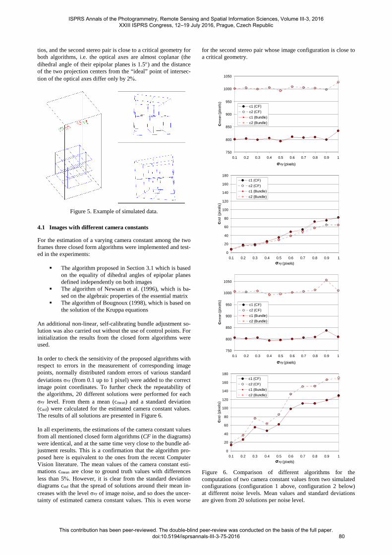
tios, and the second stereo pair is close to a critical geometry for both algorithms, i.e. the optical axes are almost coplanar (the dihedral angle of their epipolar planes is 1.5°) and the distance of the two projection centers from the “ideal” point of intersec-tion of the optical axes differ only by 2%.

Figure 5. Example of simulated data.

4.1 Images with different camera constants

For the estimation of a varying camera constant among the two frames three closed form algorithms were implemented and test-ed in the experiments:

� The algorithm proposed in Section 3.1 which is based on the equality of dihedral angles of epipolar planes defined independently on both images

� The algorithm of Newsam et al. (1996), which is ba-sed on the algebraic properties of the essential matrix

� The algorithm of Bougnoux (1998), which is based on the solution of the Kruppa equations

An additional non-linear, self-calibrating bundle adjustment so-lution was also carried out without the use of control points. For initialization the results from the closed form algorithms were used. In order to check the sensitivity of the proposed algorithms with respect to errors in the measurement of corresponding image points, normally distributed random errors of various standard deviations σxy (from 0.1 up to 1 pixel) were added to the correct image point coordinates. To further check the repeatability of the algorithms, 20 different solutions were performed for each σxy level. From them a mean (cmean) and a standard deviation (cstd) were calculated for the estimated camera constant values. The results of all solutions are presented in Figure 6. In all experiments, the estimations of the camera constant values from all mentioned closed form algorithms (CF in the diagrams) were identical, and at the same time very close to the bundle ad-justment results. This is a confirmation that the algorithm pro-posed here is equivalent to the ones from the recent Computer Vision literature. The mean values of the camera constant esti-mations cmean are close to ground truth values with differences less than 5%. However, it is clear from the standard deviation diagrams cstd that the spread of solutions around their mean in-creases with the level σxy of image noise, and so does the uncer-tainty of estimated camera constant values. This is even worse

for the second stereo pair whose image configuration is close to a critical geometry.

750

800

850

900

950

1000

1050

0.1 0.2 0.3 0.4 0.5 0.6 0.7 0.8 0.9 1

σxy (pixels)

cmea

n (p

ixel

s)

c1 (CF)

c2 (CF)

c1 (Bundle)

c2 (Bundle)

0

20

40

60

80

100

120

140

160

180

0.1 0.2 0.3 0.4 0.5 0.6 0.7 0.8 0.9 1σxy (pixels)

cstd

(pi

xels

)

c1 (CF)

c2 (CF)

c1 (Bundle)

c2 (Bundle)

750

800

850

900

950

1000

1050

0.1 0.2 0.3 0.4 0.5 0.6 0.7 0.8 0.9 1

σxy (pixels)

cmea

n (p

ixel

s)

c1 (CF)

c2 (CF)

c1 (Bundle)

c2 (Bundle)

0

20

40

60

80

100

120

140

160

180

0.1 0.2 0.3 0.4 0.5 0.6 0.7 0.8 0.9 1σxy (pixels)

cstd

(pi

xels

)

c1 (CF)

c2 (CF)

c1 (Bundle)

c2 (Bundle)

Figure 6. Comparison of different algorithms for the computation of two camera constant values from two simulated configurations (configuration 1 above, configuration 2 below) at different noise levels. Mean values and standard deviations are given from 20 solutions per noise level.



80

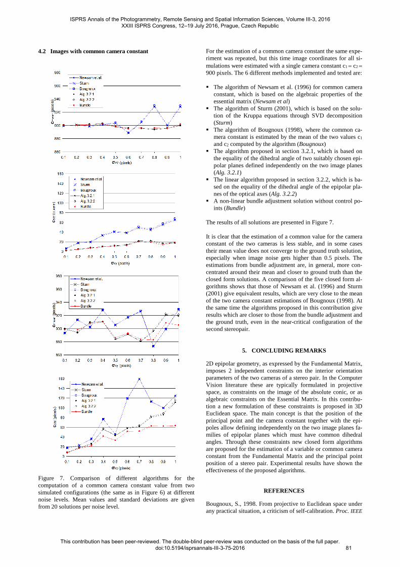
4.2 Images with common camera constant

Figure 7. Comparison of different algorithms for the computation of a common camera constant value from two simulated configurations (the same as in Figure 6) at different noise levels. Mean values and standard deviations are given from 20 solutions per noise level.

For the estimation of a common camera constant the same expe-riment was repeated, but this time image coordinates for all si-mulations were estimated with a single camera constant c1 = c2 = 900 pixels. The 6 different methods implemented and tested are: � The algorithm of Newsam et al. (1996) for common camera

constant, which is based on the algebraic properties of the essential matrix (Newsam et al)

� The algorithm of Sturm (2001), which is based on the solu-tion of the Kruppa equations through SVD decomposition (Sturm)

� The algorithm of Bougnoux (1998), where the common ca-mera constant is estimated by the mean of the two values c1

and c2 computed by the algorithm (Bougnoux) � The algorithm proposed in section 3.2.1, which is based on

the equality of the dihedral angle of two suitably chosen epi-polar planes defined independently on the two image planes (Alg. 3.2.1)

� The linear algorithm proposed in section 3.2.2, which is ba-sed on the equality of the dihedral angle of the epipolar pla-nes of the optical axes (Alg. 3.2.2)

� A non-linear bundle adjustment solution without control po-ints (Bundle)

The results of all solutions are presented in Figure 7. It is clear that the estimation of a common value for the camera constant of the two cameras is less stable, and in some cases their mean value does not converge to the ground truth solution, especially when image noise gets higher than 0.5 pixels. The estimations from bundle adjustment are, in general, more con-centrated around their mean and closer to ground truth than the closed form solutions. A comparison of the five closed form al-gorithms shows that those of Newsam et al. (1996) and Sturm (2001) give equivalent results, which are very close to the mean of the two camera constant estimations of Bougnoux (1998). At the same time the algorithms proposed in this contribution give results which are closer to those from the bundle adjustment and the ground truth, even in the near-critical configuration of the second stereopair.

5. CONCLUDING REMARKS

2D epipolar geometry, as expressed by the Fundamental Matrix, imposes 2 independent constraints on the interior orientation parameters of the two cameras of a stereo pair. In the Computer Vision literature these are typically formulated in projective space, as constraints on the image of the absolute conic, or as algebraic constraints on the Essential Matrix. In this contribu-tion a new formulation of these constraints is proposed in 3D Euclidean space. The main concept is that the position of the principal point and the camera constant together with the epi-poles allow defining independently on the two image planes fa-milies of epipolar planes which must have common dihedral angles. Through these constraints new closed form algorithms are proposed for the estimation of a variable or common camera constant from the Fundamental Matrix and the principal point position of a stereo pair. Experimental results have shown the effectiveness of the proposed algorithms.

REFERENCES

Bougnoux, S., 1998. From projective to Euclidean space under any practical situation, a criticism of self-calibration. Proc. IEEE



81

International Conference on Computer Vision, pp. 790–796.

Hartley, R., 1992. Estimation of relative camera positions for uncalibrated cameras. Proc. European Conference on Computer Vision, Springer, pp. 579-587.

Hartley, R., 1997. Kruppa's equations derived from the funda-mental matrix. IEEE Transactions on Pattern Analysis and Ma-chine Intelligence, 19(2), pp. 133-135

Hartley, R., Kaucic, R., 2002. Sensitivity of calibration to prin-cipal point position. Proc. European Conference on Computer Vision, Springer, vol. 2, pp. 433-446.

Hartley, R., Silpa-Anan, C., 2002. Reconstruction from two views using approximate calibration. Proc. Asian Conference on Computer Vision, vol. 1, pp. 338-343.

Huang, C., Chen, C., Chung, P., 2004. An improved algorithm for two-image camera self-calibration and Euclidean structure recovery using absolute quadric. Pattern Recognition, 37, pp. 1713-1722.

Kanatani, K., Matsunaga, C., 2000. Closed-form expression for focal lengths from the fundamental matrix. Proc. Asian Confe-rence on Computer Vision, vol. 1, pp. 128-133.

Kanatani, K., Nakatsuji, A., Sugaya, Y., 2006. Stabilizing the focal length computation for 3D reconstruction from two unca-librated views. The International Journal of Computer Vision, 66(2), pp. 109-122.

Li, H., 2006. A simple solution to the six-point two-view focal-length problem. Proc. European Conference on Computer Vi-sion, Springer, pp. 200-213.

Maybank S.J., Faugeras, O.D., 1992. A theory of self-calibra-tion of a moving camera. The International Journal of Compu-ter Vision, 8(2), pp. 123-151.

Newsam, G.N., Huynh, D.Q., Brooks M.J., Pan H.P., 1996. Re-covering unknown focal lengths in self-calibration: an essential-ly linear algorithm and degenerate configurations. International Archives of Photogrammetry and Remote Sensing, 31(B3), pp. 575-580.

Pan H.P., Brooks M. J., Newsam G.N., 1995. Image resituation: initial theory. Videometrics IV, Proc. SPIE, vol. 2598, pp. 162-173.

Ronda, J., Valdés, A., 2007. Conic geometry and autocalibra-tion from two images. Journal of Mathematical Imaging and Vision, 28(2), pp. 135-149.

Stewénius, H., Nister, D., Kahl, F., Schaffalitzky, F., 2005. A minimal solution for relative pose with unknown focal length. Proc. IEEE International Conference on Computer Vision and Pattern Recognition, pp. 789-794.

Sturm, P., 2001. On focal length calibration from two views. Proc. IEEE International Conference on Computer Vision and Pattern Recognition, pp. 145-150.

Sturm, P., Cheng, Z.L., Chen, P.C.Y., Poo A.N., 2005. Focal length calibration from two views: method and analysis of sin-gular cases. Computer Vision and Image Understanding, 99(1), pp. 58-95.

Whitehead A., Roth, G., 2002. Evolutionary based autocalibra-tion from the fundamental matrix. Proc. Applications of Evolu-tionary Computing on Evoworkshops. Lecture Notes in Compu-ter Science, vol. 2279, Springer, pp. 292-303.



82

Documents

A EUCLIDEAN FORMULATION OF INTERIOR ORIENTATION COSTRAINTS ...portal.survey.ntua.gr/main/labs/photo/staff/gkarras/Karras_isprs... · A EUCLIDEAN FORMULATION OF INTERIOR ORIENTATION