A DYNAMIC NEWSBOY MODEL FOR OPTIMAL RESERVE …

A DYNAMIC NEWSBOY MODEL FOR OPTIMAL RESERVE

MANAGEMENT IN ELECTRICITY MARKETS

IN-KOO CHO AND SEAN P. MEYN

Abstract. This paper examines a dynamic version of the newsboy problem in whicha decision maker must maintain service capacity from several sources to meet demandfor a perishable good, subject to the cost of providing sufficient capacity, and penaltiesfor not meeting demand. The focus application is the real-time operation of an electricpower network in which there are multiple sources of power that are distinguished bytheir cost, as well as their responsiveness in terms of ‘ramp rate’.

A complete characterization of the optimal outcome is obtained when normalized de-mand is modeled as Brownian motion. The optimal policy is affine: It is characterizedby affine switching curves in the multidimensional state space. The optimal affine pa-rameters are functions of variability in demand, production variables, and the cost ofinsufficient capacity.

Keywords: inventory theory; newsboy model; optimal control; networks; electricitymarkets; reliability.

Acknowledgements Mike Chen allowed us to use the numerical results described in Sec-tion 2.4 which are taken from his thesis [12]. We are grateful to Hungpo Chao, PeterCramton, Ramesh Johari, and Robert Wilson for helpful conversations.

Financial support from the National Science Foundation (SES-0004315, ECS-0217836,and ECS-0523620) is gratefully acknowledged. Any opinions, findings, and conclusionsor recommendations expressed in this material are those of the authors and do notnecessarily reflect the views of the National Science Foundation.

1. Introduction

Power networks throughout the world are managed through a sequence of schedulingdecisions. In various regions of the United States this task is performed by the IndependentService Operator (ISO), which serves as an impartial planner to maintain the reliabilityof the system. In the first stage, generation units are committed to serve the predictedload for the next day. Next, to ensure that power is available despite unforeseen surgesin demand, or breakdown of generation units, real-time scheduling decisions are made ontime-scales ranging from a few minutes to one hour

This paper concerns the latter real-time operation of a power network. Although thisamounts to a relatively small portion of the energy used in a typical region — in somecases less than 10% of the total energy — real-time scheduling is critical for the reliabilityof the grid. It is clear that the importance of real-time scheduling will be even greaterwith increased penetration of volatile resources such as wind, tidal, or solar power [20].

We argue that the scheduling decision problems arising in the electric power industryis the largest, and arguably the best known example of a dynamic newsboy problem. The

Date: August 25, 2010.

1

2 IN-KOO CHO AND SEAN P. MEYN

general newsboy problem concerns managing inventory for perishable goods, subject tocost for production and storage, and uncertainty in sales due to uncertainty in demand.There may also be penalties for not meeting demand. In the dynamic version of thisproblem in the case of electric power, the system operator is continuously facing thechallenge of meeting rapidly changing demand through an array of generators that canramp up rather slowly due to constraints on generation as well as the complex dynamicsof the power grid [39, 19]. Uncertainty arises from unpredictable demand, volatile supply,and failure of generation resources.

Electricity cannot be stored economically in large quantities, yet the cost of not meetingdemand is astronomical. The massive black-out seen in the Northeast on August 14, 2003,which cost $4-6 billion dollars according to the US Department of Energy, reveals thetremendous cost of service disruption [37].

Although the focus application here is electric power, we note that the dynamic newsboyproblem has application in many other settings. Examples are

Workforce management : In a large organization such as a hospital or a call center onemust maintain a large workforce to ensure effective delivery of services (see [41] for a recentacademic treatment, or IBM’s website [38].) To increase capacity of service one must bringnew employees to work. Proper talent is usually identified and trained to be placed inposition, which takes time. Alternatively, the organization can hire an employee througha temporary service agency which can offer talent at short notice, but at a higher pricethan the “usual” hiring process. In an example such as a hospital where the cost of notmeeting demand has high social cost, it is crucial to secure a reliable channel of workersthrough these means, and through on-call staff.

Fashion manufacture and retail. In supplying a seasonal fashion product, the retailermaintains a small inventory which is available at short notice, while maintaining a contractwith the supplier for deliverables in case of an unexpected surge in demand. It is moreeconomical to have such a contract than to maintain inventory, but it takes some timeto deliver the product from the producer to the retailer if demand increases unexpectedly[18].

We examine an idealized model in which a firm produces and delivers a good to theconsumer in continuous time. The good is perishable, in that it must be consumed im-mediately. This is the case in electric power or temporary services, and to a lessor extentfashionable clothing. The firm has access to a number of sources of service that can pro-duce the good. The social value is realized as the good is delivered and consumed. Onthe other hand, if some demand is not met, the social cost is proportional to the size ofthe excess demand.

It is assumed that the mean demand is met by primary service (the cheapest source ofservice capacity) through a prior contract. On-going demand can be met through primaryservice, as well as K ≥ 1 sources of ancillary service. In the case of electric power,primary service will come from coal or nuclear power generators. Gas turbine generatorsare an example of more expensive, yet more responsive sources of power providing ancillaryservice.

Other constraints and costs assumed in the model are,

• Constrained production and free disposal: Service capacity at time t from pri-mary and ancillary services are denoted {Gp(t), Ga1(t), . . . , GaK (t)}. Capacity is rate

OPTIMIZATION IN A DYNAMIC NEWSBOY MODEL 3

constrained: Gp(t) can increase at maximal rate ζp+, and Gak (t) can increase at maximalrate ζak+ < ∞. Increasing capacity takes time, but the decision maker can freely (andinstantaneously) dispose of excess capacity if desired.

• Constant marginal capacity cost: cp is the cost per unit capacity for primaryservice, and cak the cost of building one additional unit of capacity from the kth source ofancillary service. The cost parameters are ordered, cp < ca1 < · · · < caK .

• Constant marginal value of consumption: v is the value per unit capacity foroverall generation. At time t the instantaneous value of available power is v min(D(t), Gp(t)+Ga(t)), where D(t) denotes demand, and Ga(t) :=

∑i Gai(t).

• Constant marginal dis-utility of shortage: The excess capacity at time t (i.e.,the reserves), is denoted

(1.1) R(t) = Gp(t) + Ga(t) − D(t), t ≥ 0 .

The marginal cost of excess demand is denoted cbo > 0, so that the social cost of excessdemand is given by cbo max(−R(t), 0). The larger the shortage, the greater the damage tosociety. It is assumed that cbo > caK > · · · > ca1 > cp.

In practice, in particular in the case of power generation, supply is also subject to afinite downward ramping rate. However, the downward ramping rate is assumed to beconsiderably higher than the upward ramping rate — We regard the assumption of freedisposal as an idealization of a fast downward ramping rate.

The basic control problem amounts to scheduling these resources to minimize averageor discounted cost. When normalized demand is modeled as a driftless Brownian motionthe system is viewed as a (K + 1)-dimensional constrained diffusion model. The optimalpolicy is constructed explicitly through a detailed analysis of the dynamic programmingequations for the multidimensional model, and is found to be of the precise affine formintroduced in [14] (see also [46, p. 194].) The optimal solution clearly reveals how volatilityof demand and the production technology of service influences the size, the composition,and the dynamics of optimal service capacity.

1.1. Background. At the close of the 1950s, Herbert Scarf obtained the optimal policyfor a single period newsboy problem and showed that it is of a threshold form [57, 58],following previous research on inventory models by Arrow et. al. [2] and by Bellman ([8]and [7, Chapter 5].) Scarf points out in [57] that the conclusion that the solution isdefined by a threshold follows from the convexity of the value function with respect tothe decision variables. These structural issues are also developed in [7], and in dozens ofpapers published over the past fifty years (e.g. [8, 63, 31, 32, 1, 60, 61].)

Following these results there was an intense research program concerning the controlof one-dimensional inventory models, e.g. [36, 68, 56, 62, 5, 21, 54]. More recently therehave been efforts in various directions to develop hedging (or safety stocks) in multidimen-sional inventory models to improve performance [34, 27, 28, 60], make the system moreresponsive, [30]), or to obtain approximate optimality [42, 43, 33, 6, 48, 49, 50, 14, 64].

In the single-period newsboy problem, with a single source of service, the determinationof the optimal service capacity based on forecast demand can be computed through astatic calculus exercise. The resulting threshold is dependent upon cost, penalties, andthe distribution of demand (see e.g. the early work of H. Scarf [57].) Wein in [65] considers


the special case in which K = 1, and uses a similar calculation to obtain a formula foroptimal reserves in the diffusion model.

The results on optimal control obtained here are most closely related to results reportedin [14] (and developed further in [51]). It is shown that for a large class of multiclass, multi-dimensional network models, an optimal policy can be approximated in “workload space”by a generalized threshold policy. It is called an affine policy since it is constructed as anaffine translation of the optimal policy for a fluid model. In particular, [14, Theorem 4.4]establishes affine approximations under the discounted cost criterion, and [14, Proposition4.5 and Theorem 4.7] establishes similar results under the average cost criterion for adiffusion model. The method of proof reduces the optimization problem to a static opti-mization calculation based on a one-dimensional reflected Brownian motion (see also thediscussion surrounding the height process (3.35) below.) Consequently, the formula forthe optimal affine parameter obtained in [14, Proposition 4.5 and Theorem 4.7] coincideswith the formula presented in [65, Proposition 3], and is similar to the threshold valuesgiven in Section 2.2.

Some of the structural results reported in Section 2.2 are generalized in [13] to a morecomplex network setting based on an aggregate relaxation, similar to the workload relax-ations employed in the analysis of queueing models [42, 48, 51]. The results of the presentpaper and [15] were presented in part in [16], and are surveyed in the SIAM news article[55].

In all of this prior work, in the case of models of dimension greater than one, onlyapproximations of the optimal policy are obtained. The main contribution of this paperis to obtain a closed-form expression for the optimal policy, and show that it is exactly ofthe affine form that is used as an approximation in prior work.

The remainder of the paper is organized as follows. Section 2 describes the diffusionmodel in which normalized demand is a Brownian motion. The modeling assumptionsand main results of this paper are contained in Section 2: Results for the case of a singlesource of ancillary service are contained in Section 2.2, and these results are generalized tothe general model in Section 2.3. The proofs of the main results are contained in Section 3along with some extensions. Section 4 concludes the paper.

2. Dynamic Newsboy Model and Main Results

This section summarizes the main results of this paper. A diffusion model is consideredin the simplest case in which there is a single customer (also referred to as the consumer)that is served by primary and ancillary services. For the moment it is assumed that theconsumer can access only a single source of ancillary service. It is assumed that the twosources of service are owned by the same firm, simply called the supplier.

The analysis is extended to multiple sources of service in Section 2.3.

2.1. Diffusion Model. Service capacity at time t from primary and ancillary services aredenoted {Gp(t), Ga(t)}. Recall that, in application to electric power, we are consideringreal-time operations, so that the bulk of generation is scheduled in advance. The quantityGp(t) is the deviation in supply from this day-ahead scheduling, and hence it is not sign-constrained. The demand D(t) is in fact the deviation in demand from forecast, so that


it also can take on positive or negative values. However, ancillary service is not scheduledin advance, so we impose the constraint that Ga(t) ≥ 0 for all t.

Reserve at time t is defined by R(t) = Gp(t) + Ga(t) − D(t) as expressed in (1.1). Theevent R(t) < 0 is interpreted as the failure of reliable services. In the application to electricpower this represents black-out since the demand for power exceeds supply.

We sometimes refer to Gp(t)+Ga(t) as the on-line capacity, since the supplier can offerprimary and ancillary services Gp(t) and Ga(t) instantaneously at time t. Capacity issubject to ramping constraints: For finite, positive constants ζp+, ζa+,

Gp(t′) − Gp(t)

t′ − t≤ ζp+ and

Ga(t′) − Ga(t)

t′ − t≤ ζa+ for all t′ > t ≥ 0.

We assume the free disposal of capacity, which means that Gp(t) and Ga(t) can decreaseinfinitely quickly. The ramping constraints can be equivalently expressed through theequations,

(2.2) Gp(t) = Gp(0) − Ip(t) + ζp+t , Ga(t) = Ga(0) − Ia(t) + ζa+t , t ≥ 0,

where the idleness processes {Ip, Ia} are non-decreasing. It is assumed that D(0) is givenas an initial condition, and primary service is initialized using the definition (1.1),

Gp(0) = R(0) + D(0) − Ga(0).

Throughout most of the paper it is assumed that D(0) = 0.It is assumed throughout the paper that D is a driftless Brownian motion, with instan-

taneous variance denoted σ2D > 0. The model (1.1) is then called the controlled Brownian

motion (CBM) model, with two-dimensional state process X := (R,Ga)T. A Gaussianmodel for demand might be justified by considering a Central Limit Theorem scaling of alarge number of individual demand processes. Rather than attempting to justify a limitingmodel, here we choose a Gaussian demand model for the purposes of control design.

Under this assumption, the state process X evolves according to the Ito equation,

(2.3) dX = δX − BdI(t) − dDX(t), t ≥ 0 ,

where X(0) = (r, ga)T ∈ X = R×R+ is given, δX = (ζp++ζa+, ζa+)T, DX(t) = (D(t), 0)T,and the 2 × 2 matrix B is defined by,

(2.4) B =

[1 10 1

].

It is assumed that that the process I = (Ip, Ia)T appearing in (2.2) and (2.3) is adaptedto D, and that the resulting state process X is constrained to the state space X = R×R+.A process I satisfying these constraints is called admissible.

In what follows we restrict to stationary Markov policies defined as a family of admissibleidleness processes {Ix}, parameterized by the initial condition x ∈ X, with the definingproperty that the controlled process X is a strong Markov process on X.

One example of a stationary Markov policy is the affine policy that we define next. Forx ∈ R we denote,

(2.5) x+ = max(x, 0), x− = max(−x, 0) = (−x)+.

Definition 2.1. An affine policy for the CBM model (2.3) is based on a pair of thresholds(rp, ra), satisfying rp > ra > 0:


0

R

Ga

X(t)

ra rp

Figure 1: Trajectory of the two-dimensional model under an affine policy

(i) For the initial condition X(0) = x = (r, ga)T ∈ X,

(2.6) X(0+) =

(rga

)− β

(11

), ga ≥ r − rp

(rp

0

), ga ≤ r − rp

(rga

), else,

where β := min((r − ra)+, ga) ≥ 0.

(ii) For t > 0 the state process X is restricted to the smaller state space given byR(r) := closure (Rp ∪Ra), where

(2.7) Ra = {x ∈ X : x1 < ra, x2 ≥ 0}, Rp = Ra ∪ {x ∈ X : x1 < rp, x2 = 0}.(iii) For any t > 0, if R(t) < rp, then d

dtGp(t) = ζp+, and if R(t) < ra then d

dtGa(t) =

ζa+. Consequently, the following boundary constraints hold with probability one,

(2.8)

∫ ∞

0I{X(t) ∈ Rp} dIp(t) =

∫ ∞

0I{X(t) ∈ Ra} dIa(t) = 0.

⊓⊔

A sketch of a typical sample path of X under an affine policy is shown in Figure 1. Fromthe initial condition shown, the process has mean drift δX , up until the first time thatR(t) reaches the threshold ra. The subsequent downward motion shown is a consequenceof reflection at the boundary of Ra. Since R(t) remains near ra yet primary service isramped up at maximum rate ζp+, it follows that ancillary service capacity has long-runaverage drift of −ζp+ up until the first time that Ga(t) reaches zero. For the fluid modelin which σ2

D = 0 we have ddt

Ga(t) = ζa+ when R(t) < ra; ddt

Ga(t) = −ζp+ wheneverGa(t) > 0 and R(t) = ra.

2.2. Optimization. Recall that {cp, ca} denote the cost for maintaining one additionalunit of capacity for primary and ancillary services. It is assumed that the marginal costof production is higher for ancillary service,

cp < ca.


Welfare functions for the supplier and consumer are defined respectively by,

(2.9)WS(t) := (pp − cp)Gp(t) + (pa − ca)Ga(t)

WD(t) := v min(D(t), Gp(t) + Ga(t)) −(ppGp(t) + paGa(t) + cboR−(t)

).

Recall that R−(t) = max(−R(t), 0) (see (2.5)).The supplier is paid for the “on-line” capacity rather than the services delivered. For

example, in an application to power the generator may have to burn coal in order tomaintain a certain level of on-line capacity. On the other hand, the consumer obtainssurplus only from the power delivered.

The welfare function for the consumer can be simplified,

(2.10) WD(t) = vD(t) −(ppGp(t) + paGa(t) + (cbo + v)R−(t)

),

where we have used the identity,

min(D(t), Gp(t) + Ga(t)) = min(D(t), R(t) + D(t)) = D(t) − R−(t).

The social surplus at time t is given by,

W(t) = WS(t) + WD(t) .

From the identity Gp(t) = R(t)+D(t)−Ga(t), the social surplus is equivalently expressed,

W(t) = vD(t) − [cpGp(t) + caGa(t) + (cbo + v)R−(t)]

= (v − cp)D(t) − [cpR(t) + (ca − cp)Ga(t) + (cbo + v)R−(t)]

= (v − cp)D(t) − C(t),

where the cost defined by,

(2.11) C(t) := c(X(t)) := cpR(t) + (ca − cp)Ga(t) + (cbo + v)R−(t).

The mean demand takes on a constant value E[D(t)] = E[D(0)]. Hence, for a given initialcondition D(0) = d,

(2.12) E[W(t)] = (v − cp)d − E[C(t)], t ≥ 0.

In our optimization calculations we will consider the minimization of mean cost ratherthan maximization of mean welfare; this is justified by (2.12) since demand is assumed tobe exogenous. We consider the two standard optimization criteria,

Average cost: η := lim supT→∞

Ex

[ 1

T

∫ T

0c(X(t)) dt

](2.13)

Discounted cost: Jγ(x) := Ex

[∫ ∞

0e−γtc(X(t)) dt

],(2.14)

where γ > 0 is the discount parameter, and x ∈ X is the initial condition of X. Our goalis to minimize the given criterion over all stationary policies.

The steady-state cost can be computed based on the following result of [13].

Theorem 2.2. For any affine policy, the Markov process X is exponentially ergodic [22].The unique stationary distribution π on X satisfies,


(i) The first marginal of π is given by the distribution function,

Pπ{R(t) ≤ r} =

{e−θp(rp−r) ra ≤ r ≤ rp

e−θp(rp−ra)−θa(ra−r) r ≤ ra,

where

(2.15) θa = 2ζp+ + ζa+

σ2D

, θp = 2ζp+

σ2D

.

(ii) The steady state mean of the cost c : X → R+ defined in (2.11) is explicitly com-putable,

(2.16) η(r) := π(c) = θ−1a

(ζa+

ζp+ca + e−θara

(cbo + v))e−θp(rp−ra) + (rp − θ−1

p )cp.

⊓⊔

Consequently, the steady-state mean welfare functions of the supplier and consumer arecomputable when prices are fixed:

Corollary 2.3. For any affine policy the steady-state mean social surplus is finite. WhenD(0) = 0, we have

limt→∞

E[W(t)] = −η(r),

where η is given in (2.16), and the convergence is exponentially fast. Moreover, if the prices(pp, pa) are fixed, then the individual welfare functions have finite steady-state means,

limt→∞

E[WS(t)] = θ−1a

ζa+

ζp+(pa − ca)e−θp(rp−ra) + (rp − θ−1

p )(pp − cp)

limt→∞

E[WD(t)] = −[θ−1a

(ζa+

ζp+pa + e−θara

(cbo + v))e−θp(rp−ra) + (rp − θ−1

p )pp

].

When D(t) has zero-mean and the prices are fixed with pp ≤ pa ≤ cbo + v, thennecessarily E[WD(t)] < 0: Exactly as in the derivation of (2.12) we have,

E[WD(t)] = −E[ppR(t) + (pa − pp)Ga(t) + (cbo + v)R−(t)], t ≥ 0.

This is the inevitable ‘cost of variability’, i.e. risk, as seen by the consumer. Since we haveassumed that demand is normalized, the consumer sees additional value arising from thecontract purchase of mean-demand at time 0−.

An alternative is that the consumer forgoes the real-time market, trusting the ‘longterm contract’ already secured to meet mean-demand, so that Gp = Ga ≡ 0. Based on(2.9) this leads to WS(t) = 0 and

(2.17) WD(t) = −(vD−(t) + cboD+(t)

).

If D(0) = 0 this then gives,

(2.18) E[WD(t)] = −12(cbo + v)E[|D(t)|] = −1

2(cbo + v)√

tE[|D(1)|].In conclusion, although the residual mean welfare seen by the consumer is always negative,there remains much benefit to engage the supplier for services if the prices are not toohigh. As clearly shown in (2.18), the alternative ‘open-loop’ strategy is not sustainable.


12

34

56

7

1213

14

1617

18

18

20

22

24

12

34

56

7

1213

14

1617

18

18

20

22

24

15 15

CBM ModelCRW Model

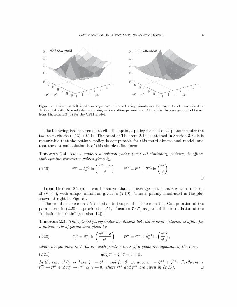
Figure 2: Shown at left is the average cost obtained using simulation for the network considered inSection 2.4 with Bernoulli demand using various affine parameters. At right is the average cost obtainedfrom Theorem 2.2 (ii) for the CBM model.

The following two theorems describe the optimal policy for the social planner under thetwo cost criteria (2.13), (2.14). The proof of Theorem 2.4 is contained in Section 3.3. It isremarkable that the optimal policy is computable for this multi-dimensional model, andthat the optimal solution is of this simple affine form.

Theorem 2.4. The average-cost optimal policy (over all stationary policies) is affine,with specific parameter values given by,

(2.19) ra∗ = θ−1a ln

(cbo + v

ca

)rp∗ = ra∗ + θ−1

p ln

(ca

cp

).

⊓⊔

From Theorem 2.2 (ii) it can be shown that the average cost is convex as a functionof (rp, ra), with unique minimum given in (2.19). This is plainly illustrated in the plotshown at right in Figure 2.

The proof of Theorem 2.5 is similar to the proof of Theorem 2.4. Computation of theparameters in (2.20) is provided in [51, Theorem 7.4.7] as part of the formulation of the“diffusion heuristic” (see also [12]).

Theorem 2.5. The optimal policy under the discounted-cost control criterion is affine fora unique pair of parameters given by

(2.20) ra∗γ = θ−1

a ln

(cbo + v

ca

)rp∗γ = ra∗

γ + θ−1p ln

(ca

cp

),

where the parameters θp, θa are each positive roots of a quadratic equation of the form

(2.21) 12σ2

Dθ2 − ζ+θ − γ = 0 .

In the case of θp we have ζ+ = ζp+, and for θa we have ζ+ = ζa+ + ζp+. Furthermorerp∗γ → rp∗ and ra∗

γ → ra∗ as γ → 0, where rp∗ and ra∗ are given in (2.19). ⊓⊔


2.3. Multiple Levels of Ancillary Service. The extension of the model to multiplesources of ancillary service contains no surprises: Suppose that there are K classes ofancillary service, with reserve capacities at time t denoted {Ga1(t), . . . , GaK (t)}. Thereserve remains defined as (1.1) with Ga(t) :=

∑i G

ai(t). The associated cost parametersand ramping rate constraints are denoted {cai , ζai+ : 1 ≤ i ≤ K} where

Gai(t′) − Gai(t)

t′ − t≤ ζai+ for all t′ > t.

It is assumed that the cost parameters are strictly increasing in the index i, with caK < cbo.The state process for control is X(t):=(R(t), Ga1(t), . . . , GaK (t))T, which is constrained

to X := R × RK+ . An affine policy is defined using the natural extension of the previous

definition: For given parameters {rp > ra1 > · · · raK} we denote

Rai := {x = (r, ga1 , . . . , gaK ) ∈ R × Rm+ : r < rai , gaj = 0 for j > i}.

The affine policy is defined so that X(t) ∈ closure (Rai) whenever Gai(t) > 0 and moreover,for each i, ∫ ∞

0I{X(t) ∈ Rai} dIai(t) = 0.

That is, Gai(t) ramps up at maximal rate when X(t) ∈ Rai .The cost function for the centralized planner is given by,

c(x) := cpr +

K∑

i=1

(cai − cp)gai + (cbo + v)r−.

We present an extension of Theorem 2.4 for the model with K levels of ancillary service.It is found that the average cost optimal policy is again affine. The analogous result inthe case of discounted cost is also valid.

In an optimal solution, capacity can sometimes be sought from a supplier with a highcost, especially if the supplier’s capacity has a high ramping rate. It can be shown thatthe introduction of a new generator will strictly reduce the value of rp∗ obtained in (2.22)whenever ζaj+ > 0.

Theorem 2.6. The average-cost optimal policy for X is affine, with specific parametervalues given in the following modification of (2.19),

(2.22)

rai∗ = rai+1∗ + 12

σ2D

ζ+i

ln

(cai+1

cai

), 1 ≤ i ≤ K,

rp∗ = ra1∗ + 12

σ2D

ζp+ln

(ca1

cp

),

where ζ+i := ζp+ +

∑j≤i ζ

aj+, and we denote cK+1 := cbo and raK+1∗ := 0. ⊓⊔

2.4. Numerical Examples. To conclude this section we present some numerical resultsbased on simulation and dynamic programming experiments. These plots are taken from[12] where the reader can find further numerical results.

Simulation and optimization are performed for a two-dimensional controlled random-walk (CRW) model which evolves in discrete time. The forecasted excess capacity at timet ≥ 1 is again defined by (1.1), where D(t) is the demand at time t, and (Gp(t), Ga(t))


rp* = 9.2

rp

ra

ra* = 2.3

= 9.2

= 2.3

rp* = 27.6

rp

ra

ra* = 6.9

= 26

= 5

rp* = 36.8

rp

ra

ra* = 9.2

= 32

= 8.3CRW model

CBM model

10- 10 0 20- 20 30

10

20

30

40

ga

10- 10 0 20- 20 30

10

20

30

40

ga

rrr

10- 10 0 20- 20 30

10

20

30

40

ga

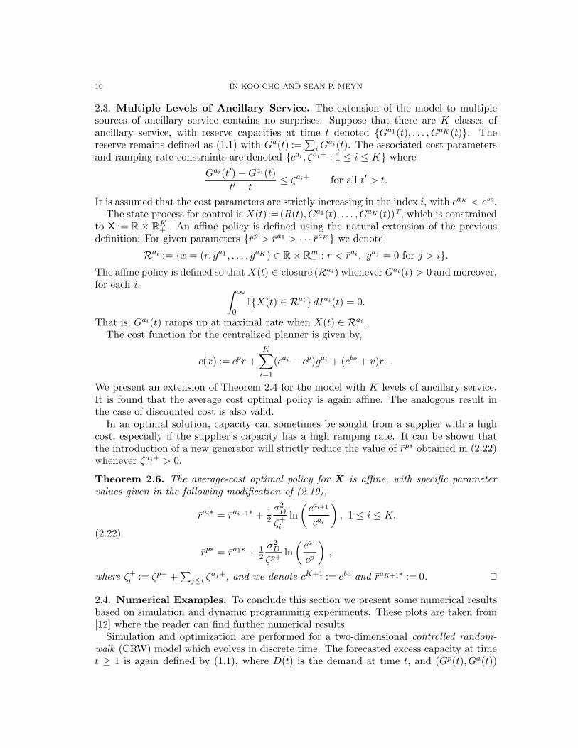
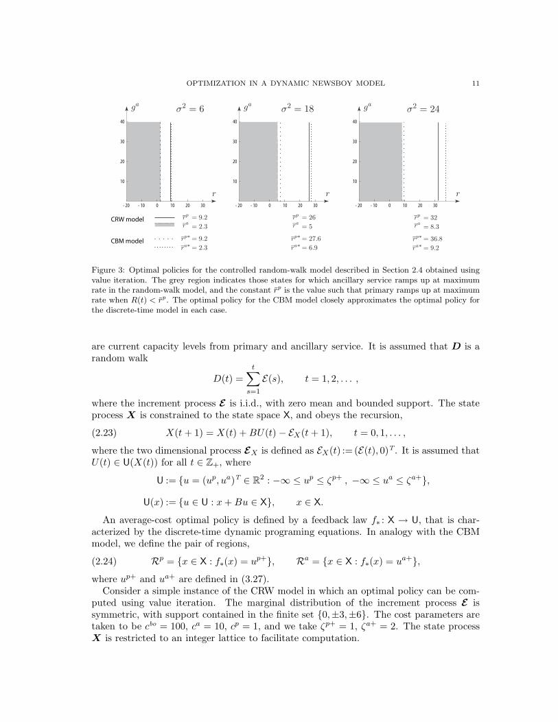
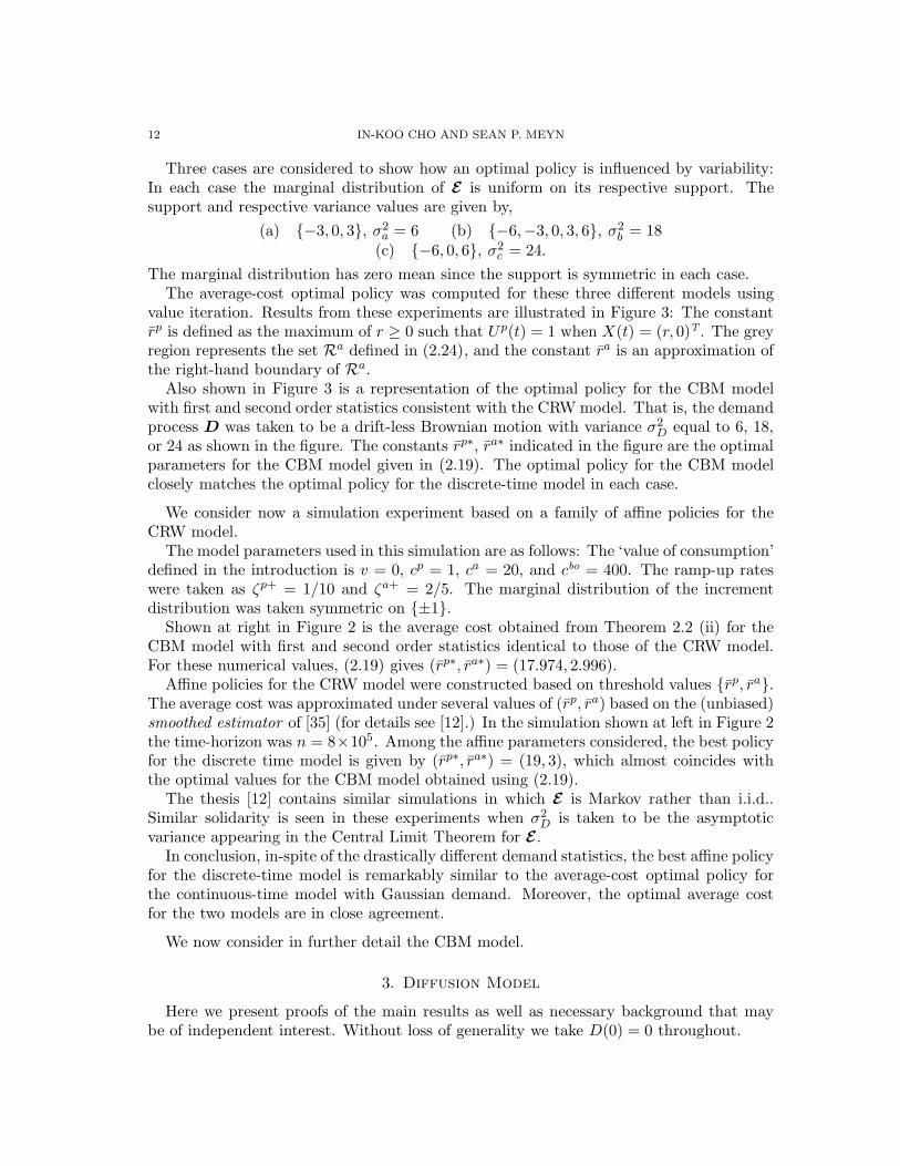
Figure 3: Optimal policies for the controlled random-walk model described in Section 2.4 obtained usingvalue iteration. The grey region indicates those states for which ancillary service ramps up at maximumrate in the random-walk model, and the constant rp is the value such that primary ramps up at maximumrate when R(t) < rp. The optimal policy for the CBM model closely approximates the optimal policy forthe discrete-time model in each case.

are current capacity levels from primary and ancillary service. It is assumed that D is arandom walk

D(t) =

t∑

s=1

E(s), t = 1, 2, . . . ,

where the increment process E is i.i.d., with zero mean and bounded support. The stateprocess X is constrained to the state space X, and obeys the recursion,

(2.23) X(t + 1) = X(t) + BU(t) − EX(t + 1), t = 0, 1, . . . ,

where the two dimensional process EX is defined as EX(t) := (E(t), 0)T. It is assumed thatU(t) ∈ U(X(t)) for all t ∈ Z+, where

U := {u = (up, ua)T ∈ R2 : −∞ ≤ up ≤ ζp+ , −∞ ≤ ua ≤ ζa+},

U(x) := {u ∈ U : x + Bu ∈ X}, x ∈ X.

An average-cost optimal policy is defined by a feedback law f∗ : X → U, that is char-acterized by the discrete-time dynamic programing equations. In analogy with the CBMmodel, we define the pair of regions,

(2.24) Rp = {x ∈ X : f∗(x) = up+}, Ra = {x ∈ X : f∗(x) = ua+},where up+ and ua+ are defined in (3.27).

Consider a simple instance of the CRW model in which an optimal policy can be com-puted using value iteration. The marginal distribution of the increment process E issymmetric, with support contained in the finite set {0,±3,±6}. The cost parameters aretaken to be cbo = 100, ca = 10, cp = 1, and we take ζp+ = 1, ζa+ = 2. The state processX is restricted to an integer lattice to facilitate computation.


Three cases are considered to show how an optimal policy is influenced by variability:In each case the marginal distribution of E is uniform on its respective support. Thesupport and respective variance values are given by,

(a) {−3, 0, 3}, σ2a = 6 (b) {−6,−3, 0, 3, 6}, σ2

b = 18(c) {−6, 0, 6}, σ2

c = 24.

The marginal distribution has zero mean since the support is symmetric in each case.The average-cost optimal policy was computed for these three different models using

value iteration. Results from these experiments are illustrated in Figure 3: The constantrp is defined as the maximum of r ≥ 0 such that Up(t) = 1 when X(t) = (r, 0)T. The greyregion represents the set Ra defined in (2.24), and the constant ra is an approximation ofthe right-hand boundary of Ra.

Also shown in Figure 3 is a representation of the optimal policy for the CBM modelwith first and second order statistics consistent with the CRW model. That is, the demandprocess D was taken to be a drift-less Brownian motion with variance σ2

D equal to 6, 18,or 24 as shown in the figure. The constants rp∗, ra∗ indicated in the figure are the optimalparameters for the CBM model given in (2.19). The optimal policy for the CBM modelclosely matches the optimal policy for the discrete-time model in each case.

We consider now a simulation experiment based on a family of affine policies for theCRW model.

The model parameters used in this simulation are as follows: The ‘value of consumption’defined in the introduction is v = 0, cp = 1, ca = 20, and cbo = 400. The ramp-up rateswere taken as ζp+ = 1/10 and ζa+ = 2/5. The marginal distribution of the incrementdistribution was taken symmetric on {±1}.

Shown at right in Figure 2 is the average cost obtained from Theorem 2.2 (ii) for theCBM model with first and second order statistics identical to those of the CRW model.For these numerical values, (2.19) gives (rp∗, ra∗) = (17.974, 2.996).

Affine policies for the CRW model were constructed based on threshold values {rp, ra}.The average cost was approximated under several values of (rp, ra) based on the (unbiased)smoothed estimator of [35] (for details see [12].) In the simulation shown at left in Figure 2the time-horizon was n = 8×105. Among the affine parameters considered, the best policyfor the discrete time model is given by (rp∗, ra∗) = (19, 3), which almost coincides withthe optimal values for the CBM model obtained using (2.19).

The thesis [12] contains similar simulations in which E is Markov rather than i.i.d..Similar solidarity is seen in these experiments when σ2

D is taken to be the asymptoticvariance appearing in the Central Limit Theorem for E .

In conclusion, in-spite of the drastically different demand statistics, the best affine policyfor the discrete-time model is remarkably similar to the average-cost optimal policy forthe continuous-time model with Gaussian demand. Moreover, the optimal average costfor the two models are in close agreement.

We now consider in further detail the CBM model.

3. Diffusion Model

Here we present proofs of the main results as well as necessary background that maybe of independent interest. Without loss of generality we take D(0) = 0 throughout.


3.1. Poisson’s equation. It is convenient to introduce two “generators” for X under agiven Markov policy. The extended generator, denoted A, is defined as follows: We writeAf = g and say that f is in the domain of A if the stochastic process M f defined belowis a local martingale for each initial condition,

(3.25) Mf (t) := f(X(t)) − f(X(0)) +

∫ t

0g(X(s)) ds, t ≥ 0.

That is, there exists a sequence of stopping times {τn} satisfying τn ↑ ∞, and for each nthe stochastic process {Mn

f (t) = Mf (t ∧ τn) : t ≥ 0} satisfies the martingale property,

E[Mnf (t + s) | Ft] = Mn

f (t), t, s ≥ 0,

where Ft = σ(X(s),D(s) : s ≤ t). See [24, 22] for background.The differential generator is defined on C2 functions f : X → R via,

(3.26) Df := 〈∇f,Bua+〉 + 12σ2

D

∂2

∂r2f,

with

(3.27) up+ = (ζp+, 0)T, ua+ = (ζp+, ζa+)T.

Suppose that X is controlled using an affine policy, and that the C2 function f satisfiesthe boundary conditions,

(3.28) 〈∇f(x), B11〉 = 0, r = rp, ga = 0, 〈∇f(x), B1

2〉 = 0, r = ra, ga ≥ 0.

where {1i} are the standard basis vectors. It then follows from Ito’s formula that f is inthe domain of A with Af = Df .

In (3.28) and throughout the paper the vector 1i denotes the ith basis vector in Eu-

clidean space.Suppose that X is defined by a Markov policy with steady-state cost η := π(c) < ∞,

where c is defined in (2.11). Poisson’s equation is then defined to be the identity,

(3.29) Ah = −c + η

The function h : X → R is known as the relative value function. If (3.29) holds then thestochastic process defined below is a local martingale for each initial condition,

(3.30) Mh(t) = h(X(t)) − h(X(0)) +

∫ t

0

(c(X(s)) − η

)ds, t ≥ 0.

The following result is an extension of results of [13], following [52, 29] and [53, Chapter17].

Define for any policy the two stopping times,

(3.31) τp := inf{t ≥ 0 : Ip(t) > 0}, τa := inf{t ≥ 0 : Ia(t) > 0}.For an affine policy with thresholds ra < rp these stopping times have the equivalentrepresentation,

τp = inf{t ≥ 0 : R(t) ≥ rp}, τa = inf{t ≥ 0 : R(t) ≥ ra}.In this case it is shown that the function h : X → R defined as

(3.32) h(x) = Ex

[∫ τp

0

(c(X(t)) − η

)dt

], x ∈ X ,


solves Poisson’s equation for X, where η(r) is defined in Theorem 2.2.

Proposition 3.1. Suppose that X is controlled using an affine policy. Then,

(i) The following bound holds for each m ≥ 2, some constant bm < ∞, and any stoppingtime τ satisfying τ ≤ τp,

Ex

[‖X(τ)‖m +

∫ τ

0‖X(t)‖m−1 dt

]≤ bm(‖x‖m + 1) x ∈ X .

(ii) One solution to Poisson’s equation is given by (3.32). Moreover, for this solutionthe stochastic process Mh is a martingale.

(iii) The function h given in (3.32) satisfies for some b0 < ∞,

−b0 ≤ h(x) ≤ b0(‖r − ga‖2 + 1), x ∈ X.

Proof. Part (i) is a minor extension of the proof of Proposition A.2 in [13]. Parts (ii) and(iii) are given in [13, Proposition A.2].

Since the proof is short we include a proof of (i): Consider for m ≥ 2 the C2 functionVm(x) := m−1|r − ga − rp|m, x = (r, ga)T ∈ X. Applying the differential generator (3.26)we obtain,

DVm (x) = −ζp+|r − ga − rp|m−1 + σ2D(m − 1)|r − ga − rp|m−2, x ∈ R(r) ,

where R(r) is defined above (2.7). This function also satisfies the boundary conditionsgiven in (3.28) since m ≥ 2, so that Vm is in the domain of A and AVm = DVm (thisfollows from Ito’s formula — See [24, Theorem 2.9, p. 287], [23, 59] and their references).Consequently, one can find a compact set Sm ⊂ X, cm < ∞, and εm > 0 such that,

AVm ≤ −εmVm−1 + cmISm , on R(r).

The bound in (i) then follows from standard arguments (see [13, Proposition A.2] and also[52]). ⊓⊔

3.2. Height process. Proposition 3.1 asserts that the function h defined in (3.32) is asolution to Poisson’s equation. To prove Theorem 2.4 we construct representations for thegradient of h in terms of the stopping times defined in (3.31), and the pair of sensitivityfunctions,

(3.33)λp(x) = 〈∇c(x), B1

1〉 = cp − I{r ≤ 0}cbo,

λa(x) = 〈∇c(x), B12〉 = ca − I{r ≤ 0}cbo .

The analysis is based upon a reduction to a pair of one-dimensional reflected processes:the height processes with respect to each of the thresholds rp, ra,

Hp(t) := rp − R(t) + Ga(t),(3.34)

Ha(t) := ra − R(t), t ≥ 0 .(3.35)

We have Hp(t) ≥ 0 for all t > 0 under the affine policy, and moreover,

dHp (t) = −ζp+dt + dIp(t) + dD(t), t ≥ 0.

Hence Hp is a one-dimensional reflected Brownian motion (RBM), and Ha evolves as anRBM up until the first time that Ga(t) = 0.


To analyze these height processes we first present some results for a standard RBMsatisfying the the Ito equation,

(3.36) dH = −δH dt − dI(t) + dD(t), t ≥ 0 ,

where D is a driftless Brownian motion, and the reflection process I is non-decreasingand satisfies, ∫ ∞

0I{H(t) > 0} dI(t) = 0.

When δH > 0 the Markov process H is positive recurrent, and its unique invariant prob-ability measure is exponential with parameter θH := 2δH/σ2

H [11].For a given constant r0 ≥ 0 define

τr0= min{t ≥ 0 : H(t) = r0}

and consider the convex, C1 function defined by,

(3.37) Ψ(r) =

{eθHr − θHr r < r0

eθHr0 − θHr0 + mH(r − r0) r ≥ r0,

where mH = Ψ′(r0) = θH(eθHr0 − 1).

Proposition 3.2. Suppose that the reflected Brownian motion has negative drift so thatδH > 0. Then for each initial condition H(0) = r ≥ 0,

(i) E[τ0] = δ−1H r.

(ii) For any r0 ≥ r,

P{τr0< τ0} = (eθHr0 − 1)−1(eθHr − 1).

(iii) For any constant r0 > 0,

(3.38) Ex

[∫ τ0

0I{H(t) ≥ r0} dt

]=

(Ψ(r) − 1 + θHr

)(δHθHeθHr0

)−1.

Proof. These formulae can be found in or derived from results in [11]. In particular (ii) isgiven as formula 3.0.4 (b), p. 309, and (iii) follows from formula 3.46 (a), p. 313 of [11].We provide a brief proof based on invariance equations for the differential generator,

DH = −δH∇ + 12σ2

H∇2.

To prove (i) let g(r) = δ−1H r so that DHg = −1. It follows that Mi(t) = t∧τ0+g(H(t∧τ0))

is a martingale,

E[t ∧ τ0 + δ−1H H(t ∧ τ0)] = E[Mi(t)] = E[Mi(0)] = δ−1

H H(0).

Letting r → ∞ and applying the Dominated Convergence Theorem gives (i).The function g : R+ → R+ defined by g(r) := eθHr, r ∈ R, is in the null space of the

differential generator for H , which implies that Mii(t) = eθHH(t∧τ0) is a local martingale.Uniform integrability can be established to conclude that with τ = min(τr0

, τ0),

E[Mii(τ)] = Mii(0), 0 ≤ r ≤ r0.

Rearranging terms gives (ii).To see (iii) we apply the differential generator to Ψ to obtain,

DHΨ = −δH

(−θHIr<r0

+ mHIr≥r0

).


Here we have again used the fact that DHg = 0. Substituting the definition of mH andwriting Ir<r0

+ Ir≥r0= 1 then gives,

DHΨ = δH

(θH − (mH + θH)Ir≥r0

).

The function Ψ satisfies Ψ′(0) = 0, so we can replace DH by AH in the expressionabove, which means that the process defined below is a local martingale,

Miii(t) := Ψ(H(t)) − δH

∫ t

0

(θH − (mH + θH)IH(s)≥r0

)ds, t ≥ 0.

It is in fact a martingale since it is uniformly integrable on any bounded interval. It isalso uniformly integrable on [0, τ0] which implies that,

Ψ(r) = Miii(0) = E[Miii(τ0)] = Ψ(0) − δHE

[∫ τ0

0

(θH − (mH + θH)I{H(s) ≥ r0}

)ds

]

Rearranging terms gives for any r0 > 0,

E

[∫ τ0

0I{H(s) ≥ r0} ds

]=

(δH(mH + θH)

)−1(Ψ(r) − Ψ(0) + δHθHE[τ0]

).

The expression (3.38) then follows. ⊓⊔

Based on the foregoing we now show that the function h defined in (3.32) is smooth.We consider the normalized function h•(x) = h(x) − h(xp), x ∈ X, with xp := (rp, 0)T.We obtain a useful representation for h• through a particular construction of the stateprocesses starting from various initial conditions. Based on a single Brownian motion D,we define on the same probability space the entire family of solutions to (2.3), denoted{X(t;x) : t ≥ 0, x ∈ X}.

The processes X(t;x) and X(t;xp) have corresponding height processes Hp(t;x), Hp(t;xp)satisfying Hp(0;xp) = 0 and Hp(0;x) ≥ 0. Consequently, the two processes couple at timeτp(x) = min{t : Hp(t;x) = 0} = min{t : Hp(t;x) = Hp(t;xp)}. This combined with (3.32)implies the representation,

(3.39)

h•(x) = Ex

[∫ τp(x)

0

(c(X(t;x)) − c(X(t;xp))

)dt

]

= Ex

[∫ ∞

0

(c(X(t;x)) − c(X(t;xp))

)dt

], x ∈ X .

In Proposition 3.3, the function (3.39) is compared to the function obtained when X

is replaced by the fluid model in which σ2D = 0. This deterministic process is denoted

x = (r,ga)T, and satisfies for t > 0,

d

dtx(t;x) =

Bua+ r(t;x) < ra;

Bua− r(t;x) = ra, ga(t;x) > 0;

Bup+ ra ≤ r(t;x) < rp, ga(t;x) = 0;

0 r(t;x) = rp,

where up+ and ua+ are defined in (3.27), and ua− = (ζp+,−ζp+)T. The potential jump attime t = 0 is identical to its stochastic counterpart (see (2.6).)


Proposition 3.3. Suppose that X is controlled using an affine policy and that h• isdefined by (3.39). Denote by h0 the corresponding function when D = 0,

(3.40) h0(x) =

∫ ∞

0

(c(x(t;x)) − c(xp)

)dt x ∈ X .

Then,

(i) The function h0 is C1, and satisfies,

Dh0 = −c + c(xp) + 12σ2

D

∂2

∂r2h0.

(ii) The function h• has the explicit form,

h• = h0 + ℓ + m

where ℓ is a continuous piecewise-linear function of (r, ga)T, and m is a piecewiseexponential function of r. The following identities hold whenever the derivatives aredefined.

Dℓ = −(c(xp) + 1

2σ2D

∂2

∂r2h0

)+ η, Dm = 0.

(iii) h• is C1 and satisfies the boundary conditions,

(3.41)

∂

∂rh• (x) +

∂

∂gah• (x) = 0, when r ≥ ra;

∂

∂rh• (x) = 0, when r + ga ≥ rp.

Proof. The proof of Part (i) is similar to Proposition 4.2 of [50]. We first establish that h0

is smooth. A representation of the derivative is obtained by differentiating the expressionfor h0:

∇h0(x) =

∫ ∞

0∇c(x(t;x)) dt x ∈ X ,

where the derivative is with respect to the initial condition x. Following arguments in[50], it can be shown that this expression is continuous and piecewise-linear on X. Theexpression 〈∇h0 (x), Bua+〉 = −c(x) + c(xp) follows from the Fundamental Theorem ofCalculus and the representation,

h0(x(s;x)) =

∫ ∞

s

(c(x(t;x)) − c(xp)

)dt x ∈ X ,

and this completes the proof of (i).Parts (ii) and (iii) are proved in Appendix A of Chen’s thesis [12]. The explicit formulae

require complex computations, but the qualitative results are straightforward: We havefrom (i),

Dh0 = −c + b0,

where b0 is piecewise constant. Following the proof of (i) we can give an explicit expressionfor ℓ,

ℓ(x) =

∫ τ0p

0

(b0(x(t;x)) − η

)dt x ∈ X ,


where τ0p = Hp(0;x)/ζp+ = (rp − r + ga)/ζp+. This function is piecewise-linear and

continuous, and satisfies,Dℓ = −b0 + η,

whenever ℓ is differentiable. Hence h0 + ℓ satisfies Poisson’s equation for the differen-tial generator. The function m is in the null space of the differential generator, and isconstructed so that h0 + ℓ + m is C1. It is of the specific form,

m(r) =

Ap + Bpe−θpr ra ≤ r ≤ rp;

Aa + Bae−θar 0 ≤ r < ra;

Aa + Ba r < 0,

where the parameters {θa, θp} are defined in (2.15), and (Aa, Ap, Ba, Bp) are constants. ⊓⊔

We can now obtain representations of the derivatives:

Proposition 3.4. Under an affine policy using any thresholds rp, ra, the directionalderivatives of the function h defined in (3.32) can be expressed as follows for x ∈ R(r),

〈∇h(x),12〉 = −Ex

[∫ τp

0λp(X(t)) dt

]

= −cpE[τp] + ca

Ex

[∫ τa

0I{R(t) ≤ ra} dt

](3.42)

〈∇h(x), B12〉 = Ex

[∫ τa

0λa(X(t)) dt

]

= caE[τa] − cbo

Ex

[∫ τa

0I{R(t) ≤ 0} dt

].

(3.43)

Proof. We omit the proof of (3.42) since it is similar (and simpler) than the proof of (3.43).Equation (3.43) is based on the following representation of h,

(3.44) h(x) = Ex

[∫ τa

0

(c(X(t)) − η

)dt + h(X(τa))

], x ∈ X.

This follows from the martingale property for Mh and the bound Proposition 3.1 (i) withm = 3 (which implies that the martingale is uniformly integrable on [0, τa].)

Suppose that X(0) = x lies in the interior of Ra(r) and consider the perturbationXε(0) = xε := x − εB1

2 for small ε > 0. The state processes {Xε : ε ≥ 0} are defined ona common probability space, with common demand process D. We then have,

Xε(t) = X(t) − εB12, 0 ≤ t ≤ τa,

and from (3.44) it follows that for all x ∈ X,

(3.45) h(x)−h(xε) = Ex

[∫ τa

0

(c(X(t))−c(X(t)−εB1

2))dt+h(X(τa))−h(X(τa)−εB1

2)].

Proposition 3.3 and the Mean Value Theorem give,

|h(X(τa)) − h(X(τa) − εB12)| = ε|〈∇h(X), B1

2〉|,where X = X(τa) − εB1

2 for some ε ∈ (0, ε). We have R(τa) = ra, which implies that

|〈∇h(X), B12〉| → 0 with probability one as ε → 0.


An application of Proposition 3.3 (iii) gives the following bound,

sup0≤ε≤1

‖∇h(y − εB12)‖ ≤ b0‖y‖, y = (ra, ga), ga ≥ 0,

where the constant b0 is independent of ga. Proposition 3.1 (i) with m = 3 implies uniformintegrability, so that

limε→0

E[|〈∇h(X), B12〉|] = 0.

Multiplying the identity (3.45) by ε−1 and applying Proposition 3.1 (i) once more gives,

limε→0

ε−1(h(x) − h(xε)) = Ex

[∫ τa

0limε→0

ε−1(c(X(t)) − c(X(t) − εB1

2))dt

], x ∈ Ra(r),

which gives (3.43). ⊓⊔

3.3. Optimization. In this section we apply Proposition 3.1 to show that the affine policydescribed in Theorem 2.4 is average-cost optimal. The treatment of the discounted caseis identical - we omit the details.

The dynamic programing equations for the CBM model are written as follows,

Average cost:(Dh∗ + c − η∗

)∧

(inf

{〈∇h∗(x),−Bu〉 : u ∈ R

2+

})= 0(3.46)

Discounted cost:(DK∗ + c − γK∗

)∧

(inf

{〈∇K∗(x),−Bu〉 : u ∈ R

2+

})= 0(3.47)

where the differential generator D is defined in (3.26) (see [3, 4, 10]). The function h∗ : X →R+ in (3.46) is known as the relative value function, and η∗ is the optimal average cost.For the models considered here, however, we do not know if these value functions are C2

on all of X. Hence the dynamic programing equation (3.46) or (3.47) is interpreted in theviscosity sense [26, 17] (alternatively, one can replace D by A in these definitions.)

The relative value function defines a constraint region for X as follows: Define inanalogy with (2.7),

Rp = {x ∈ X : 〈∇h∗(x), B11〉 < 0}, Ra = {x ∈ X : 〈∇h∗(x), B1

2〉 < 0}.Then, with R∗ :=closure {Ra∪Rp}, the optimal policy maintains for each initial condition,

(3.48) (i) X(t) ∈ R∗ for all t > 0, (ii) With probability one (2.8) holds.

A representation for h∗ can be obtained through a generalization of the “stochasticshortest path” formulation of [25] to the continuous time case (see also [66, 67, 9, 45], andin particular [47, Theorem 1.7] where the extensions to continuous time are spelled-out.)Consider for any x ∈ X,

h◦(x) := inf Ex

[∫ τp

0(c(X(t)) − η∗) dt

],

where the stopping time τp is defined for a general policy in (3.31), and the infimum isover all admissible I. Under the optimal policy, the value function h◦ solves the same


martingale problem as h∗, that is Ah◦ = −c + η∗. It is the unique solution to (3.46) (upto an additive constant) over all functions with quadratic growth.1

Conversely, if a solution to (3.46) can be found with quadratic growth then this definesan optimal policy:

Proposition 3.5. Suppose that (3.46) holds for a function h∗ satisfying for some b0 < ∞,

−b0 ≤ h∗(x) ≤ b0(1 + ‖x‖2), x ∈ X.

Then for any Markov policy that gives rise to a positive recurrent process X with invariantprobability measure π we have

∫c(x)π(dx) ≥ η∗. Moreover, this lower bound is attained

for the process defined in R∗ satisfying (3.48).

Proof. Proposition 3.5 is a minor extension of [45, Theorem 5.2]. We sketch the proofhere.

The essence of the dynamic programming equation (3.46) is that the process defined by

Mh∗(t) = h∗(X(t)) − h∗(X(0)) +

∫ t

0

(c(X(s)) − η∗

)ds, t ≥ 0,

is a local submartingale for any solution X obtained using an admissible idleness processI: There exists a sequence of stopping times {τn} satisfying τn ↑ ∞, and the stochasticprocess defined by Mn

h∗

(t) = Mh∗(t ∧ τn) satisfies the sub-martingale property,

E[Mnh∗

(t + s) | Ft] ≥ Mnh∗

(t), t, s ≥ 0.

We can in fact take τn = min{t ≥ 0 : h∗(X(t)) ≥ n}. From the Monotone ConvergenceTheorem we obtain the bound,

(3.49) Ex

[h∗(X(t)) +

∫ t

0c(X(s)) ds

]≥ tη∗ + h∗(x), t ≥ 0, x ∈ X.

That is, the modifier ‘local’ can be removed: Mh∗is a sub-martingale.

Arguments used in [45, Theorem 5.2] imply that the following limit holds for a.e. x ∈ X

[π] whenever π(c) < ∞,

limt→∞

t−1Ex[h∗(X(t))] = lim

t→∞t−1

Ex[‖X(t)‖2] = 0.

Consequently, letting t → ∞ in (3.49) gives, for a.e. X(0) = x ∈ X,

η = limt→∞

t−1Ex

[∫ t

0c(X(s)) ds

]≥ η∗.

Moreover, if X is defined under the optimal policy then Mh∗is a local martingale since

Poisson’s equation holds,

(3.50) Ah∗ = −c + η∗.

If h∗ has quadratic growth then Mh∗is a martingale (see prior footnote), and hence (3.49)

can be strengthened to an equality,

Ex

[h∗(X(t)) +

∫ t

0c(X(s)) ds

]= tη∗ + h∗(x), t ≥ 0, x ∈ X.

1Uniqueness is established in [45, Theorem A3]. Although stated in discrete time, Section 6 of [45]describes how to translate to continuous time. Related results are obtained for constrained diffusions in[3].


This shows that∫

c(x)π(dx) = η∗ under the policy defined in (3.48). ⊓⊔

We can now state the main result of this section. Recall that the thresholds rp∗ and ra∗

are defined in (2.19).

Proposition 3.6. The following hold for the CBM model under an affine policy:

(i) Suppose that primary service is specified using the threshold rp > ra∗. If ra = ra∗

then the solution to Poisson’s equation (3.32) satisfies,

〈∇h(x), B12〉 < 0, x ∈ Ra.

(ii) If rp = rp∗ and ra = ra∗ then h satisfies in addition,

〈∇h(x), B11〉 < 0, x ∈ Rp.

Consequently, h solves the dynamic programming equation (3.46).

Corollary 3.7. For any given rp > ra∗, the optimal policy over all Ga is the affine policyobtained using the same ra∗.

Proof of Proposition 3.6. Recall that under an affine policy, Hp is a one-dimensionalRBM. For an initial condition x ∈ R(r) satisfying ga = Ga(0) > 0, the height process Hp

evolves as a one-dimensional RBM up to the first time t > 0 that Ga(t) = 0.

Part (i). We begin by considering the right hand side of (3.43). We show that this isstrictly negative on Ra(r) when ra = ra∗ through an analysis of the height process Ha.

The gradient formula (3.43) can be expressed in terms of the height process (3.35) via,

(3.51) 〈∇h(x), B12〉 = ca

E[τa] − cboEx

[∫ τa

0I{Ha(t) ≥ ra} dt

].

The stopping time τa can be interpreted as the first hitting time to the origin for Ha. Thefollowing identities are obtained in Proposition 3.2:

E[τa] = δ−1H r, Ex

[∫ τa

0I{Ha(t) ≥ ra} dt

]=

(Ψ(r) − 1 + θHr

)(δHθHeθH ra

)−1,

where Ψ is defined in (3.37) by

Ψ(r) =

{eθHr − θHr r < r0

eθHr0 − θHr0 + mH(r − r0) r ≥ r0,

with r0 = ra, r = Ha(0) = ra − r ≥ 0, and δH = ζp+ + ζa+. Consequently, (3.51) can beexpressed,

〈∇h(x), B12〉 = Φ(r) := caδ−1

H r − cbo

(Ψ(r) − 1 + θHr

)(δHθHeθH ra

)−1, r ≥ 0.

The function Ψ is convex, with Ψ(0) = 1 and Ψ′(0) = 0. Consequently, the function Φdefined above is concave, strictly concave on [0, ra], with Φ(0) = 0. To show that Φ isnegative on (0,∞) it suffices to show that Φ′(0) ≤ 0.

The derivative at zero is expressed,

Φ′(0) = caδ−1H − cbo

(Ψ′(0) + θH

)(δHθHeθH ra

)−1= δ−1

H

(ca − cboe−θH ra

).

When ra = ra∗ we have e−θH ra

= ca/cbo, so that Φ′(0) = 0.


Part (ii). We next consider 〈∇h,B11〉 for x ∈ Ra when rp∗ and ra∗ are given by (2.19).

Consider the height process relative to rp defined in (3.34). By the foregoing analysiswe have on Ra,

〈∇h, 11 + 12〉 = 〈∇h,B1

2〉 < 0.

Consequently, to show that 〈∇h,B11〉 < 0 it is sufficient to show that 〈∇h, 12〉 ≥ 0. This

derivative is given in (3.42), which can be expressed in terms of the height process,

〈∇h, 12〉 = caE

[∫ τp

0I{Hp(t) ≥ r0} dt

]− cp

E[τp],

where r0 = rp − ra. Proposition 3.2 then gives, with r = Hp(0),

〈∇h, 12〉 = ca(Ψ(r) − 1 + θHr

)(δHθHeθHr0

)−1− cpδ−1

H r.

The drift parameter for Hp is δH = ζp+. The parameter rp∗ is chosen so that eθHr0 = ca/cp,which on substitution gives,

(3.52) 〈∇h, 12〉 = cpδ−1H

(θ−1H

(Ψ(r) − 1 + θHr

)− r

)= cpδ−1

H θ−1H

(Ψ(r) − 1

).

For r ≥ r0 > 0 (equivalently, r < ra), we obtain from the definition of Ψ,

〈∇h, 12〉 ≥ cpδ−1H θ−1

H

(eθHr0 − θHr0 − 1

)> 0.

We conclude that 〈∇h, 11〉 < 0 on Ra.

Finally we demonstrate that 〈∇h,B11〉 < 0 on Rp \Ra. For an initial condition x ∈ Rp

satisfying ra ≤ r < rp we can write,

h(x) = Ex

[∫ τ

0

(c(X(t)) − η

)dt + h(X(τ))

]

where τ = min(τa, τp). Recall that 〈∇h(x), 11〉 = 0 if τ = τp. Consequently, using familiararguments,

〈∇h(x), 11〉 = E[cpτ + 〈∇h(X(τ)), 11〉

]

= E[(

cpτa + 〈∇h(xa), 11〉)I{τa ≤ τp} + cpτpI{τa > τp}

],

where xa = (ra, 0)T. On rearranging terms and applying the strong Markov property weobtain,

〈∇h(x), 11〉 = cpEx[τp] +

(〈∇h(xa), 11〉 − cp

Exa [τp])P{τa > τp} .

Consideration of the height process Hp then gives,

(3.53) 〈∇h(x), 11〉 = cpδ−1H r +

(〈∇h(xa), 11〉 − cpδ−1

H r0

)P

H{τr0> τ0},

where r0 = rp − ra and the probability on the right hand side is with respect to the heightprocess: Proposition 3.2 gives P

H{τr0< τ0} = (eθHr0 − 1)−1(eθHr − 1).

Equation (3.52) provides an expression for the derivative of h at xa,

〈∇h(xa), 11〉 = −〈∇h(xa), 12〉 = −cpδ−1H θ−1

H

(eθHr0 − θHr0 − 1

).

Combining this identity with (3.53) we obtain,

〈∇h, 11〉 = cpδ−1H

(r − θ−1

H

(eθHr0 − 1

)P

H{τr0> τ0}

)

= cpδ−1H

(r − θ−1

H

(eθHr − 1

)), 0 ≤ r ≤ r0.


The right hand side is strictly negative for r > 0. ⊓⊔

The proof of Theorem 2.6 is identical to the simpler setting of Section 3.3. We demon-strate that the solution to Poisson’s equation h under the affine policy solves the dynamicprograming equation,

(Dh∗ (x) + c − η∗

)∧

(inf

{〈∇h∗(x),−Bu〉 : u ∈ R

K+1+

})= 0, x ∈ X,

where here we let B denote the (K +1)×m matrix defined by B(1, i) = 1 = B(i+1, i) = 1for each i, and B(i, j) = 0 for all other indices (i, j).

Proof of Theorem 2.6. The proof that 〈∇h(x), B1i〉 is non-positive for i = 1 and i = K+1

is identical to the proof of Theorem 2.4. To obtain the analogous result for i ∈ {2, . . . ,m}we apply similar reasoning. Exactly as in (3.43), it can be shown that for x ∈ Rai ,

(3.54) 〈∇h(x), B1i+1〉 = caiE[τai

] − cai+1Ex

[∫ τai

0I{R(t) ≤ rai+1} dt

],

where τai:= inf{t ≥ 0 : R(t) = rai}.

To compute the right hand side of (3.54) we again construct a one-dimensional Brownianmotion to represent these expectations. Define for R(0) = q < rai ,

Hai(t) := rai − R(t) +∑

j>i

Gaj (t), t ≥ 0.

This is described by,

dHai(t) = −ζ+i dt + dIai(t) + dD(t), t ≥ 0 while Gai(t) > 0.

Consequently, we can write using (3.54),

(3.55) 〈∇h(x), B1i+1〉 = caiE[τai

] − cai+1Ex

[∫ τai

0I{Hai(t) ≥ (rai − rai+1)} dt

],

and τaicoincides with the first hitting time to the origin for Hai . Consequently, applying

Proposition 3.2,

〈∇h(x), B1i+1〉 = caiδ−1

H r − cai+1

(Ψ(r) − 1 + θHr

)(δHθHeθH(rai−rai+1)

)−1, r ≥ 0,

where θH = 2ζ+i /σ2

D, and the function Ψ is defined in (3.37). The remainder of the proof

is identical to the proof of Proposition 3.6 using the formula e−θH rai = cai/cai+1 . ⊓⊔

4. Conclusions

Theorem 2.4 establishes an explicit formula for reserves in the dynamic newsboy model.Optimal reserves are high whenever there is high variability in demand, or significantramping constraints on production. These conclusions are (qualitatively) consistent withthe substantial reserves maintained in any major power market.

Many conclusions are reasonably robust to modeling assumptions. An investigation ofthe impact of uncertainty of supply is carried out in [44] based on ideas in this paper.Some preliminary numerical studies to investigate the impact of correlation are containedin [12]. In most cases a Brownian model predicts with reasonable accuracy approximatevalues for optimal hedging points, where the variance chosen in the diffusion model is theasymptotic variance for a discrete model (i.e. the Central Limit Theorem variance.)


Our focus in current research is the decentralized market problem, for which Theo-rem 2.4 and Theorem 2.5 have clear implications: If the prices {cp, ca} are the pricescharged to the consumer by the supplier, the supplier will assume that the consumer willoptimize based on what it is charged. The formulae given in these two theorems quantifythe observation: When θp is small, then the fair price for ancillary service may be ex-tremely high. The parameter θp is small if there is significant variability in demand, or ifthe maximum ramp-up rate for primary service is small. This is an important observationcritical for interpreting a market outcome sustaining the optimal allocation [15, 44].

It is a task of fundamental importance to build robust market rules that can withstandconsiderable volatility and possible strategic manipulation by the players. We need to movebeyond a static analysis in order to address issues surrounding reliability and dynamics ina market setting.

References

[1] E. Altman, B. Gaujal, and A. Hordijk. Multimodularity, convexity, and optimization properties. Math.Oper. Res., 25(2):324–347, 2000.

[2] K. J. Arrow, Theodore Harris, and Jacob Marschak. Optimal inventory policy. Econometrica, 19:250–272, 1951.

[3] R. Atar and A. Budhiraja. Singular control with state constraints on unbounded domain. Ann. Probab.,34(5):1864–1909, 2006.

[4] Rami Atar, Amarjit Budhiraja, and Ruth J. Williams. HJB equations for certain singularly controlleddiffusions. Adv. Appl. Probab., 17(5-6):1745–1776, 2007.

[5] C. Bell. Characterization and computation of optimal policies for operating an M/G/1 queuing systemwith removable server. Operations Res., 19:208–218, 1971.

[6] S. L. Bell and R. J. Williams. Dynamic scheduling of a system with two parallel servers in heavy trafficwith complete resource pooling: Asymptotic optimality of a continuous review threshold policy. Ann.Appl. Probab., 11:608–649, 2001.

[7] R. Bellman. Dynamic Programming. Princeton University Press, Princeton, NJ, 1957.[8] R. Bellman, I. Glicksberg, and O. Gross. On the optimal inventory equation. Management Sci., 2:83–

104, 1955.[9] D. P. Bertsekas. A new value iteration method for the average cost dynamic programming problem.

SIAM J. Control Optim., 36(2):742–759 (electronic), 1998.[10] V. Borkar and A. Budhiraja. Ergodic control for constrained diffusions: characterization using HJB

equations. SIAM J. Control Optim., 43(4):1467–1492 (electronic), 2004/05.[11] A. N. Borodin and P. Salminen. Handbook of Brownian motion—facts and formulae. Probability and

its Applications. Birkhauser Verlag, Basel, first (second ed. published 2002) edition, 1996.[12] M. Chen. Modelling and control of complex stochastic networks, with applications to manufacturing

systems and electric power transmission networks. PhD thesis, University of Illinois at Urbana Cham-paign, University of Illinois, Urbana, IL, USA, 2005.

[13] M. Chen, I.-K. Cho, and S.P. Meyn. Reliability by design in a distributed power transmission network.Automatica, 42:1267–1281, August 2006. (invited).

[14] M. Chen, C. Pandit, and S. P. Meyn. In search of sensitivity in network optimization. Queueing Syst.Theory Appl., 44(4):313–363, 2003.

[15] I.-K. Cho and S. P. Meyn. Efficiency and marginal cost pricing in dynamic competitive markets. Toappear in J. Theo. Economics, 2006.

[16] I.-K. Cho and S. P. Meyn. Optimization and the price of anarchy in a dynamic newsboy model.Stochastic Networks, invited session at the INFORMS Annual Meeting, November 13-16, 2005.

[17] M. G. Crandall, H. Ishii, and P.-L. Lions. User’s guide to viscosity solutions of second order partialdifferential equations. Bull. Amer. Math. Soc. (N.S.), 27(1):1–67, 1992.

[18] P. Dasgupta, L. Moser, and P. Melliar-Smith. Dynamic pricing for time-limited goods in a supplier-driven electronic marketplace. Electronic Commerce Research, 5:267–292, 2005.


[19] C. L. DeMarco. Electric power network tutorial: Basic steady state and dynamic models for control,pricing, and optimization. http://www.ima.umn.edu/talks/ workshops/3-7.2004/demarco/IMA Power Tutorial 3 2004.pdf, 2004.

[20] E.A. DeMeo, G.A. Jordan, C. Kalich, J. King, M.R. Milligan, C. Murley, B. Oakleaf, and M.J.Schuerger. Accommodating wind’s natural behavior. Power and Energy Magazine, IEEE, 5(6):59 –67,Nov.-Dec. 2007.

[21] B. T. Doshi. Optimal control of the service rate in an M/G/1 queueing system. Adv. Appl. Probab.,10:682–701, 1978.

[22] D. Down, S. P. Meyn, and R. L. Tweedie. Exponential and uniform ergodicity of Markov processes.Ann. Probab., 23(4):1671–1691, 1995.

[23] P. Dupuis and R. J. Williams. Lyapunov functions for semimartingale reflecting Brownian motions.Ann. Appl. Probab., 22(2):680–702, 1994.

[24] S. N. Ethier and T. G. Kurtz. Markov Processes : Characterization and Convergence. John Wiley &Sons, New York, 1986.

[25] A. Federgruen, A. Hordijk, and H. C. Tijms. Denumerable state semi-Markov decision processes withunbounded costs, average cost criterion unbounded costs, average cost criterion. Stoch. Proc. Applns.,9(2):223–235, 1979.

[26] W. H. Fleming and H. M. Soner. Controlled Markov processes and viscosity solutions, volume 25 ofApplications of Mathematics (New York). Springer-Verlag, New York, 1993.

[27] S. B. Gershwin. Manufacturing Systems Engineering. Prentice–Hall, Englewood Cliffs, NJ, 1993.[28] S.B. Gershwin. Production and subcontracting strategies for manufacturers with limited capacity and

volatile demand. IIE Transactions on Design and Manufacturing, 32(2):891–906, 2000. Special Issueon Decentralized Control of Manufacturing Systems.

[29] P. W. Glynn and S. P. Meyn. A Liapounov bound for solutions of the Poisson equation. Ann. Probab.,24(2):916–931, 1996.

[30] S. C. Graves. Safety stocks in manufacturing systems. J. Manuf. Oper. Management, 1(1):67–101,1988.

[31] B. Hajek. Optimal control of two interacting service stations. IEEE Trans. Automat. Control, AC-29:491–499, 1984.

[32] B. Hajek. Extremal splittings of point processes. Math. Oper. Res., 10(4):543–556, 1985.[33] J. M. Harrison and J. A. Van Mieghem. Dynamic control of Brownian networks: state space collapse

and equivalent workload formulations. Ann. Appl. Probab., 7(3):747–771, 1997.[34] J.M. Harrison. The BIGSTEP approach to flow management in stochastic processing networks, pages

57–90. Stochastic Networks: Theory and Applications. Oxford University Press, Oxford, UK, 1996.[35] S. G. Henderson, S. P. Meyn, and V. B. Tadic. Performance evaluation and policy selection in mul-

ticlass networks. Discrete Event Dynamic Systems: Theory and Applications, 13(1-2):149–189, 2003.Special issue on learning, optimization and decision making (invited).

[36] D.P. Heyman. Optimal operating policies for M/G/1 queueing systems. Operations Res., 16:362–382,1968.

[37] P. Hines, J. Apt, and S. Talukdar. Trends in the history of large blackouts in the united states. InProc. of the 2008 IEEE Power and Energy Society General Meeting - Conversion and Delivery ofElectrical Energy in the 21st Century, pages 1 –8, jul. 2008.

[38] IBM. Call center analytics and optimization.http://domino.research.ibm.com/odis/odis.nsf/pages/micro.01.02.html, 2005.

[39] M. Ilic and J. Zaborszky. Dynamics and Control of Large Electric Power Systems. Wiley-Interscience,New York, 2000.

[40] P. L. Joskow and J. Tirole. Reliability and Competitive Electricity Market. IDEI, University ofToulouse, 2004.

[41] D. L. Kaufman, H.-S. Ahn, and M. E. Lewis. On the introduction of an agile, temporary workforceinto a tandem queueing system. Queueing Syst. Theory Appl., 51:135–171, 2005.

[42] F.P. Kelly and C.N. Laws. Dynamic routing in open queueing networks: Brownian models, cut con-straints and resource pooling. Queueing Syst. Theory Appl., 13:47–86, 1993.

[43] L. F. Martins, S. E. Shreve, and H. M. Soner. Heavy traffic convergence of a controlled, multiclassqueueing system. SIAM J. Control Optim., 34(6):2133–2171, November 1996.


[44] S. Meyn, M. Negrete-Pincetic, G. Wang, A. Kowli, and E. Shafieepoorfard. The value of volatileresources in electricity markets. In Proc. of the 49th Conf. on Dec. and Control, pages 4921–4926,Atlanta, GA, 2010.

[45] S. P. Meyn. The policy iteration algorithm for average reward Markov decision processes with generalstate space. IEEE Trans. Automat. Control, 42(12):1663–1680, 1997.

[46] S. P. Meyn. Stability and optimization of queueing networks and their fluid models. In Mathematicsof stochastic manufacturing systems (Williamsburg, VA, 1996), pages 175–199. Amer. Math. Soc.,Providence, RI, 1997.

[47] S. P. Meyn. Stability, performance evaluation, and optimization. In E. Feinberg and A. Shwartz,editors, Markov Decision Processes: Models, Methods, Directions, and Open Problems, pages 43–82.Kluwer, Holland, 2001.

[48] S. P. Meyn. Sequencing and routing in multiclass queueing networks. Part II: Workload relaxations.SIAM J. Control Optim., 42(1):178–217, 2003.

[49] S. P. Meyn. Dynamic safety-stocks for asymptotic optimality in stochastic networks. Queueing Syst.Theory Appl., 50:255–297, 2005.

[50] S. P. Meyn. Workload models for stochastic networks: Value functions and performance evaluation.IEEE Trans. Automat. Control, 50(8):1106–1122, August 2005.

[51] S. P. Meyn. Control Techniques for Complex Networks. Cambridge University Press, Cambridge, 2007.[52] S. P. Meyn and R. L. Tweedie. Generalized resolvents and Harris recurrence of Markov processes.

Contemporary Mathematics, 149:227–250, 1993.[53] S. P. Meyn and R. L. Tweedie. Markov chains and stochastic stability. Cambridge University Press,

Cambridge, second edition, 2009. Published in the Cambridge Mathematical Library. 1993 editiononline: http://black.csl.uiuc.edu/~meyn/pages/book.html.

[54] B. Mitchell. Optimal service-rate selection in an M/G/1 queue. SIAM J. Appl. Math., 24(1):19–35,1973.

[55] Sara Robinson. Math model explains volatile prices in power markets. SIAM News, Oct. 2005.[56] S. M. Ross. Arbitrary state Markovian decision processes. Ann. Math. Statist., 39(1):2118–2122, 1968.[57] H. E. Scarf. The optimality of (S, s) policies in the dynamic inventory problem. In Mathematical

methods in the social sciences, 1959, pages 196–202. Stanford Univ. Press, Stanford, Calif., 1960.[58] Herbert E. Scarf. Some remarks on Bayes solutions to the inventory problem. Naval Res. Logist.

Quart., 7:591–596, 1960.[59] E. Schwerer. A linear programming approach to the steady-state analysis of reflected Brownian motion.

Stoch. Models, 17(3):341–368, 2001.[60] S. P. Sethi and G. L. Thompson. Optimal Control Theory: Applications to Management Science and

Economics. Kluwer Academic Publishers, Boston, 2000.[61] S.P. Sethi, H. Yan, J.H. Yan, and H. Zhang. An analysis of staged purchases in deregulated time-

sequential electricity markets. Journal of Industrial and Management Optimization, 1:443–463, No-vember 2005.

[62] M. J. Sobel. Optimal average-cost policy for a queue with start-up and shut-down costs. OperationsRes., 17:145–162, 1969.

[63] S. Stidham, Jr. and R. Weber. A survey of Markov decision models for control of networks of queues.Queueing Syst. Theory Appl., 13(1-3):291–314, 1993.

[64] A. L. Stolyar. Maxweight scheduling in a generalized switch: state space collapse and workload mini-mization in heavy traffic. Adv. Appl. Probab., 14(1):1–53, 2004.

[65] L. M. Wein. Dynamic scheduling of a multiclass make-to-stock queue. Operations Res., 40(4):724–735,1992.

[66] P. Whittle. Optimization over time. Vol. I. Wiley Series in Probability and Mathematical Statistics:Applied Probability and Statistics. John Wiley & Sons Ltd., Chichester, 1982. Dynamic programmingand stochastic control.

[67] P. Whittle. Optimization over time. Vol. II. Wiley Series in Probability and Mathematical Statistics:Applied Probability and Statistics. John Wiley & Sons Ltd., Chichester, 1983. Dynamic programmingand stochastic control.

[68] M. Yadin and P. Naor. Queueing systems with a removable service station. Operations ResearchQuarterly, 14(4):393–405, 1963.


Department of Economics, University of Illinois, 1206 S. 6th Street, Champaign, IL 61820

USA

E-mail address: [email protected]

URL: http://www.business.uiuc.edu/inkoocho

Coordinated Science Laboratory and Department of Electrical and Computer Engineer-

ing, University of Illinois, 1308 W. Main Street, Urbana, IL 61801 USA

E-mail address: [email protected]

URL: https://netfiles.uiuc.edu/meyn/www/spm.html

Documents

A DYNAMIC NEWSBOY MODEL FOR OPTIMAL RESERVE …