Embed Size (px)
Citation preview
A Dynamic Model of Network Formation with StrategicInteractions
Michael D. Koniga, Claudio J. Tessonea, Yves Zenoub
aChair of Systems Design, Department of Management, Technology and Economics,ETH Zurich, Kreuzplatz 5, CH-8032 Zurich, Switzerland
bStockholm University and Research Institute of Industrial Economics (IFN). Sweden.
Abstract
In order to understand the different characteristics observed in real-worldnetworks, one needs to analyze how and why networks form, the impactof network structure on agents’ outcomes, and the evolution of networksover time. For this purpose, we combine a network game introduced byBallester et al. [2006], where the Nash equilibrium action of each agent isproportional to her Bonacich centrality [Bonacich, 1987], with an endoge-nous network formation process. Links are formed on the basis of agents’centrality while the network is exposed to a volatile environment introducinginterruptions in the connections between agents. We show that there existsa unique stationary network whose topological properties completely matchfeatures exhibited by real-world networks. We also find that there exists asharp transition in efficiency and network density from highly centralized todecentralized networks.
Key words: Bonacich centrality, network formation, network games,nested split graphsJEL: C63, D83, D85, L22
1. Introduction
Social networks are important in several facets of our lives. For exam-ple, the decision of an agent of whether or not to buy a new product, attenda meeting, commit a crime, find a job is often influenced by the choicesof his or her friends and acquaintances. The emerging empirical evidence
We are greatful for comments from Patrick Groeber, Matthew Jackson, FernandoVega-Redondo, Sanjeev Goyal, Jan Bramoulle, Mateo Marsili, Guido Caldarelli, UlrikBrandes, and participants at the DIME conference in Paris 2009 and the Summer Schoolon Innovation and Networks in Trento 2009, where earlier versions of this paper have beenpresented.
Email addresses: [email protected] (Michael D. Konig), [email protected] (ClaudioJ. Tessone), [email protected] (Yves Zenou)
September 11, 2009
on these issues motivates the theoretical study of network effects. For ex-ample, job offers can be obtained from direct, and indirect, acquaintancesthrough word-of-mouth communication. Also, risk-sharing devices and co-operation usually rely on family and friendship ties. Spread of diseases, suchas AIDS infection, also strongly depends on the geometry of social contacts.If the web of connections is dense, we can expect higher infection rates. Interms of structure, real-life networks are characterized by low diameter (theso-called “small world” property), high clustering, and “scale-free” degreedistributions.
To fathom these different aspects and to match the observed structureof real-life networks, one needs to analyze how and why networks form,the impact of network structure on agents’ outcomes, and the evolution ofnetworks over time. The aim of the present paper is to propose a theoreticalmodel that has all these features.
The literature on network formation is basically divided in two strandsthat are not communicating very much with each other. In the randomnetwork approach (mainly developed by mathematicians and physicists),1
which is mainly dynamic, the reason why a link formed is pure chance.Indeed, this literature builds networks either through a purely stochasticprocess where links appear at random according to some distribution, or elsethrough some algorithm for building links. In the other approach (developedby economists), which is mainly static, the reason for the formation of a linkis strategic interactions. Individuals carefully decide with whom to interactand this decision entails some consent by both parts in a given relationship.2
As Jackson [2007, 2008] pointed out, the random approach gives us a greatdeal of insight into how networks form (i.e. matches the characteristics ofreal-life networks) while the deterministic approach performs better on whynetworks form.3
There is also another strand of literature (called “games on networks”)which takes the network as given and study how the network structure im-pacts on outcomes and individual decisions. A prominent paper of this liter-ature is Ballester et al. [2006].4 They mainly show that if agents’ payoffs are
1See Albert and Barabasi [2002].2See Jackson [2007, 2008] for a complete overview of these two approaches.3Most of models of strategic network formation are static. Two prominent exceptions
include Jackson and Watts [2002b] and Dutta et al. [2005]. Jackson and Watts [2002b]model network formation as an intertemporal process with myopic individuals breakingand forming links as the network evolves dynamically. Individuals are myopic in the sensethat their decisions are guided completely by current payoffs, although the process ofnetwork formation takes place over real time. Dutta et al. [2005] relax this assumption andassume that agents behave in a farsighted manner by taking into account the intertemporalrepercussions of their own decisions.
4 Bramoulle and Kranton [2007] and Galeotti et al. [2009] are also important papers inthis literature. The former focuses on local substitutabilities between agents connected in
2

linear-quadratic, then the unique interior Nash equilibrium of an n−playergame in which agents are embedded in a network is such that each individ-ual effort is proportional to her Bonacich centrality measure. The latter isa well-known centrality measure introduced by Bonacich [1987].5 In otherwords, it is mainly the centrality of an agent in a network that explains heroutcome.6
To the best of our knowledge, there are very few papers that combine theliterature on network formation and games on networks.7 This is the aimof the present paper and, as we will show, combining these two approacheswill allow us to match the characteristics of most real-life networks.
To be more precise, we develop a two-stage game where, in the firststage, as in Ballester et al. [2006], agents play their equilibrium contribu-tions proportional to their Bonacich centrality while, in the second stage, arandomly chosen agent can update her linking strategy by creating a newlink as a local best response to the current network. Furthermore, agentsare embedded in a volatile environment which requires them to continuallyadapt to changing conditions. We assume that a link of a randomly selectedagent decays, i.e. can be severed.
As a result, the formation of social networks can be regarded as a tensionbetween the search for new linking opportunities and volatility that leadsto the decay of existing links. Let us be more precise about each of the twomechanisms: (i) link creation and (ii) link decay.
(i) We assume that a randomly selected agent in the network creates alink with the agent with the highest centrality among the neighbors ofher neighbors (the second order neighbors). This means that the valueof each link is not an exogenous parameter but rather depends on the
a network while the latter provides a model where agents do not have perfect informationabout the network. As in the present paper, Ballester et al. [2006] analyze a network gameof local complementarities under perfect information
5Centrality is a fundamental measure of the importance of actors in social networks,dating back to early works such as Bavelas [1948]. See Wasserman and Faust [1994] foran introduction and survey.
6In the empirical literature, it has been shown that centrality is important in explainingexchange networks [Cook et al., 1983], peer effects [Calvo-Armengol et al., 2009; Durlauf,2004; Haynie, 2001], creativity of workers [Perry-Smith and Shalley, 2003], workers’ per-formance [Mehra et al., 2001], power in organizations [Brass, 1984], the flow of information[Borgatti, 2005; Stephenson and Zelen, 1989], the formation and performance of R&D col-laborating firms and inter-organizational networks [Boje and Whetten, 1981; Powell et al.,1996; Uzzi, 1997] as well as the success of open-source projects [Grewal et al., 2006].
7Notable exceptions are Bramoulle et al. [2004], Cabrales et al. [2009],Calvo-Armengol and Zenou [2004], Galeotti and Goyal [2009], Goyal and Vega-Redondo[2005], Jackson and Watts [2002a]. Contrary to our approach, all these models are static,and are unable to reproduce the main characteristics of real-world networks. Also, thenetwork formation process is very different.
3
structure of the social network given by the centrality of an agent.8
(ii) The volatility of the environment is an essential feature of our model.It may affect the value of a connection and, in turn, make it unprof-itable. Moreover, volatility expresses the fact that there exist con-straints on the number of links an agent can maintain. Similar toother authors (e.g. Ehrhardt et al. [2008, 2006b], Marsili et al. [2004],Vega-Redondo [2006]), we therefore assume that a link of a randomlyselected agent decays. However, differently to these works, we do notassume that links decay at an exogenously given rate that is constantfor all links connecting agents. Instead, we assume that agents viewthe links to the most central agents in their neighborhood as morevaluable than the links to agents with low centrality. Under these con-ditions, agents use more valuable links more frequently. On the otherhand, less frequently used links are exposed to stochastic link decay.As a result, less frequently used links decay before more frequentlyused links are disrupted.9
As in Jackson and Rogers [2007], we then proceed by showing that ourmodel reproduces the main empirical observations of social networks. In-deed, we show that the stationary networks emerging in our link formationprocess are characterized by short path length with high clustering (so called“small worlds”, see Watts and Strogatz [1998]), exponential degree distribu-tions with power law tails and negative degree-clustering correlation. Thesenetworks also show a clear core-periphery structure. Moreover, we showthat, if agents have no “budget constraints”and can form any number oflinks then stationary networks are dissortative. However, if one takes intoaccount capacity constraints in the number of links an agent can maintain,and allows for random global attachment between agents, we keep all theabove mentioned network statistics while, at the same time, yielding assor-tative stationary networks.
Apart from reproducing empirically observed patterns, we demonstrateunder which conditions these networks emerge and that there exists a sharptransition between hierarchical and flat network structures. Instead of re-lying on a mean-field approximation of the degree distribution and related
8 We further show that among all the possible links to second order neighbors the linkto the one with the highest centrality increases the centrality (and thus the utility) ofboth agents (the initiator and the target of the link) the most. Thus agents do not onlyconnect to agents with high centrality but they also strive to maximize their own centrality(and thus their own utility). In this broader sense we can view the link formation processas a competition for high centrality. Finally, we incorporate congestion and capacityconstraints in the number of links an agent can maintain. This leads to the fact thatagents with many links who have been identified as a linking source or target can refuseto create or accept a link.
9Thus, we assume that the link of an agent i to the neighbor with the lowest centralitydecays with a rate qi.
4

measures as all these models do, we are able to derive explicit solutionsfor all network statistics of the stationary network (by computing the ad-jacency matrix) in the absence of capacity constraints in the number oflinks an agent can maintain. We also observe that the network architectureadapts to changes in the volatility of the environment. We also find that,by altering the rate at which linking opportunities arrive and links decay,a sharp transition takes place in the network density. In line with previousworks [Arenas et al., 2008; Guimera et al., 2002; Visser, 2000], this transi-tion entails a crossover from highly centralized networks when the linkingopportunities are rare and the link decay is high to highly decentralizednetworks when many linking opportunities arrive and only few links are re-moved. From the efficiency perspective such sharp transition can also beobserved in aggregate payoffs in stationary networks.
The paper is organized as follows. In Section 2, we introduce the modeland discuss the basic properties of the network formation process. In par-ticular, Section 2.1 discusses the first stage of the game. In Section 2.2,we introduce the second stage of the game, where the network formation isexplained. Next, Section 3 shows that stationary networks exist and can becomputed analytically. After deriving the stationary networks, in Section4, we analyze their properties in terms of topology and centralization. InSection 5, we study efficiency from the point of view of maximizing totalefforts and aggregate payoff in the stationary network. We investigate theefficiency of different stationary networks as a function of the volatility ofthe environment. Section 6 discusses our results and their robustness, es-pecially when we consider very general utility functions. Appendix A givesall the necessary definitions and characterizations of general networks. InAppendix B, we focus on a class of networks (nested split graphs) that areimportant in our analysis and provide a general discussion in terms of theirtopology properties and centralization measures. We extend our analysisin Appendix C by including capacity constraints in the number of links anagent can maintain and a global search mechanism for new linking partners.Finally, all proofs can be found in Appendix D.
2. The model
In this section, we develop a two-stage game. In the first stage, fol-lowing Ballester et al. [2006], all agents simultaneously choose their effortlevel in a fixed network structure. It is a game with local complementaritieswhere players have linear-quadratic payoff functions. In the second stage, arandomly chosen agent decides with whom she wants to form a link whilea volatile environment forces the least frequently used link of a randomlyselected agent to decay. This introduces two different time scales, one inwhich agents are choosing their efforts in a simultaneous move game andthe second in which an agent forms a link as a best response to the current
5
network. in which each agent chooses an effort level. We assume that thetime in which agents are forming new links evolves much slower than therate at which the stage game is repeated (see Vega-Redondo [2006], for asimilar approach).
2.1. Nash Equilibrium and Bonacich CentralityConsider a static network G in which the nodes represent a set of agents/players
N = 1, 2, ..., n. Following Ballester et al. [2006], each agent i = 1, ..., n inthe network G selects an effort level xi ≥ 0, x ∈ R
n+, and receives a payoff
πi(x1, ..., xn) of the following form
πi(x1, ..., xn) = xi −1
2x2
i + λn∑
j=1
aijxixj . (1)
This utility function is additively separable in the idiosyncratic effort compo-nent (xi− 1
2x2i ) and the peer effect contribution (λ
∑nj=1 aijxixj). Payoffs dis-
play strategic complementarities in effort levels, i.e., ∂2πi(x1, ..., xn)/∂xi∂xj =λaij ≥ 0. In order to find the Nash equilibrium solution associated with theabove payoff function, we define a network centrality measure introducedby Bonacich [1987]. Let A be the symmetric n× n adjacency matrix of thenetwork G and λPF its largest real eigenvalue. We have:
Definition 1. The matrix B(G, λ) = (I−λA)−1 exists and is non-negativeif and only if λ < 1/λPF.10 Then
B(G, λ) =∞∑
k=0
λkAk.
The Bonacich centrality vector is given by
b(G, λ) = B(G, λ) · u, (2)
where u = (1, ..., 1)T .
We can write the Bonacich centrality vector as
b(G, λ) =∞∑
k=0
λkAk · u = (I − λA)−1 · u.
For the components bi(G, λ), i = 1, ..., n, we get
bi(G, λ) =∞∑
k=0
λk(Ak · u)i =∞∑
k=0
λkn∑
j=1
a[k]ij , (3)
10The proof can be found e.g. in Debreu and Herstein [1953].
6
where a[k]ij is the ij-th entry of Ak. Because
∑nj=1 a
[k]ij is the number of all
walks of length k in G starting from i, bi(G, λ) is the number of all walksin G starting from i, where the walks of length k are weighted by theirgeometrically decaying factor λk.
Now we can turn to the equilibrium analysis of the game.
Theorem 1 (Ballester et al. [2006]). Let b(G, λ) be the Bonacich net-work centrality of parameter λ. For λ < λPF, the unique interior Nashequilibrium solution of the simultaneous n–player move game with payoffsgiven by (1) and strategy space R
n+ is given by
x∗i = bi(G, λ), (4)
for all i = 1, ..., n.
Moreover, the payoff of agent i in the equilibrium is given by
πi(x∗, G) =
1
2(x∗
i )2 =
1
2b2i (G, λ). (5)
The parameter λ measures the effect on agent i of agent j’s contribution,if they are connected. If we assume that we have strong network externali-ties so that λ approaches its highest possible value 1/λPF then the Bonacichcentrality becomes proportional to the standard eigenvector measure of cen-trality [Wasserman and Faust, 1994]. The latter result has been shown byBonacich [1987] and Bonacich and Lloyd [2001].
Furthermore, Ballester et al. [2006] have shown that the equilibrium out-come and the payoff for each player increases with the number of links in G(because the number of network walks increases in this way).11 This impliesthat, if an agent is given the opportunity to change her links, she will add asmany links as possible. On the other hand, if she is only allowed to form onelink at a time, she will form the link to the agent that increases her payoffthe most. In both cases, eventually, the network will then become complete,i.e. each agent is connected to every other agent. However, to avoid thislatter unrealistic situation, we assume that the agents are living in a volatileenvironment that causes links to decay such that the complete network cannever be reached. Instead the architecture of the network adapts to thevolatile environment. We will treat these issues more formally in the nextsection.
2.2. The Network Formation Game
We now introduce a network formation process that incorporates theidea that agents with high Bonacich centrality (their equilibrium effort lev-els) are more likely to connect to each other [Gulati and Gargiulo, 1999;
11See their Theorem 2.
7
Nerkar and Paruchuri, 2005] and that the presence of common neighborsenhances the likelihood of agents to form a new link between them [Gulati,1995].
Let time be measured at countable dates t = 0, 1, 2, .... The timing is asfollows. At t = 0, we start with the empty network G(0). Then every agentoptimally chooses her effort, which is x∗
i = 1, for all i = 1, ..., n since there isno link. Then, an agent i is chosen at random and with probability pi formsa link with agent j that gives her the highest utility (or equivalently herhighest Bonacich centrality). We obtain the network G(1). Then, again, aplayer i is chosen at random and with probability pi decides with whom shewants to form a link. For that, she has to calculate all the possible networkconfigurations and chooses the one that gives her the highest utility. An soforth.
Let us now explain the game in more detail and, in particular, the for-mation of links between agents. Let Ni = k ∈ N : ik ∈ L(t) be the set
of neighbors of agent i ∈ N and N (2)i =
⋃
j∈NiNj\ (Ni ∪ i) denote the
second-order neighbors of agent i in the current network G(t) = (N, L(t)).We assume that agents form links only with the neighbors of their neigh-bors. Quite naturally, if an agent has no links, then she will search amongall agents for the best links. We make this assumption because agents knowmainly their friends and the friends of their friends. In the friendship exam-ple, individuals connect to friends of friends because they trust their ownfriends who can recommend them to their acquaintances. Also, each indi-vidual is likely to meet a friend of friend and thus decides to create a linkor not. More generally, it seems reasonable that the formation of links islimited to agents that someone is aware of. This should be even more true inlarge networks where players’ information may be limited to their immediate“neighborhood”.12
The key question is how individuals choose among their second-orderneighbors (i.e. friends of friends). Let us explain the way someone is selectedto form a link. At every t, an agent i, selected uniformly at random fromthe set N , enjoys an updating opportunity of her current links at a ratepi ∈ (0, 1). If an agent receives such an opportunity, then she initiates a linkto agent j which increases her equilibrium payoff the most in her second-
order neighborhood N (2)i . Agent j is said to be the local best response of
agent i given the network G(t). Agent j accepts the link if i has also thehighest centrality in her second-order neighborhood. That is, agent i isalso a local best response of agent j. The underlying assumption for thisis that individuals carefully decide with whom to interact and this decisionentails some consent by both parts in a given relationship. Note, that the
12In Appendix C, we allow agents to create links with agents further away in the network,i.e. at length greater than two.
8
connectivity relation is symmetric such that j is a second-order neighbor ofi if i is a second order neighbor of j. Moreover, as we will see below, agenti is always a local best response of agent j if agent j is a local best responseof agent i.
Observe that when agents decide to create a link, they do it in a myopicway, that is they only look at the second-order neighbor that gives themthe current highest utility. There is literature on farsighted networks whereagents calculate their lifetime-expected utility when they want to create alink (see, e.g. Konishi and Ray [2003]). We adopt here a myopic approachbecause of its tractability and because our model also incorporates effortdecision.13
Let us give a formal definition of the local best responses of an agentgiven the prevailing network G(t).14
Definition 2. Consider the current network G(t) with agents N = 1, ..., n.Let G(t) + ij be the graph obtained from G(t) by the addition of the edgeij /∈ G(t) between agents i ∈ N and j ∈ N . Further, let π∗(G(t)) =(π∗
1(G(t)), ..., π∗n(G(t))) denote the profile of Nash equilibrium payoffs of the
agents in G(t) following from the payoff function (1) with parameter λ <1/λPF(G(t)). Then agent j is a local best response of agent i if π∗
i (G(t) +
ij) ≥ π∗i (G(t) + ik) for all j, k ∈ N (2)
i . Agent j may not be unique. The setof agent i’s local best responses is denoted by BRi(G(t)). If agent i does not
have any second-order neighbors, N (2)i = ∅, then agent j is a local best re-
sponse of agent i if π∗i (G(t)+ij) ≥ π∗
i (G(t)+ik) for all j, k ∈ N\ (Ni ∪ i).
Note that the best response strategies for the network games introduced inBala and Goyal [2000]; Haller et al. [2007]; Haller and Sarangi [2005] allowan agent to remove or create an arbitrary number of links while we restrictthe link formation (strategy space) of an agent to one additional link only.We omit the removal of links since agents payoffs are monotonic increasingin the number of links in the network. Since the removal of a link wouldalways decrease an agent’s payoffs, link removal is strictly dominated by linkcreation.
We assume that during the time interval from t to t + 1 an agent i isselected and either has the possibility to create a link (with probability pi)or to severe a link (with probability qi). Note that taking into account thepossibility of an agent remaining quiescent only modifies the time-scale of
13Jackson and Watts [2002b] argue that this form of myopic behavior makes sense ifplayers discount heavily the future.
14In order to guarantee an interior solution of the Nash equilibrium efforts correspondingto the payoff functions in (1) we assume that the parameter λ is smaller than the inverse ofthe largest real eigenvalue of G(t) for any t. Testing the impact of the Bonacich centralitymeasure on educational outcomes in the United States, Calvo-Armengol et al. [2009] foundthat only 18 out of 199 networks (i.e. 9 percent) do not satisfy this eigenvalue condition.
9
the process discussed, thus yielding identical results to the model proposed.This implies that, without any loss of generality, it is possible to assumepi + qi = 1. For simplicity, we also assume that these probabilities are thesame across agents. Accordingly, we will use one parameter α and 1 − α todenote the probabilities at which links are formed and removed respectively.
Definition 3. We define the network formation process (G(t))∞t=0 as a se-quence of networks G(0), G(1), G(2), ... in which at every step t = 0, 1, 2, ...,an agent i is uniformly selected at random, i ∼ U1, ..., n. Then one of thefollowing two events occurs:
(i) With probability α ∈ (0, 1) agent i initiates a link to a local bestresponse agent j ∈ BRi(G(t)). Then the link ij is created if i ∈BRj(G(t)) is a local best response of j, given the current network G(t).If BRi(G(t)) = ∅ or BRj(G(t)) = ∅ nothing happens. If BRi(G(t)) isnot unique, then i selects randomly one agent in BRi(G(t)).
(ii) With probability 1−α the link ij ∈ G(t) is removed such that π∗i (G(t)−
ij) ≤ π∗i (G(t) − ik) for all j, k ∈ Ni. If agent i does not have any link
then nothing happens.
In words, with probability α, the selected agent will create a link with hersecond-order neighbor who increases the most her utility, while with proba-bility 1−α, the selected agent will delete a link with her direct neighbor whoreduces the least her utility. This link is for the selected agent the least im-portant and thus the least frequently used. Note that the newly establishedlink also affects the overall network structure and therewith the centralitiesand payoffs of all other agents (in the same connected component). Theformation of links thus can introduce large, unintended and uncompensatedexternalities.
2.3. Network Formation and Nested Split Graphs
An essential property of the link formation process (G(t))t∈Nintroduced
in Definition 3 is that it produces a well defined class of graphs denotedby “nested split graphs ” [Aouchiche et al., 2006].15 We will give a formaldefinition of these graphs and discuss an example in this section. Nestedsplit graphs include many common networks such as the star or the completenetwork. Moreover, as their name already indicates, they have a nestedneighborhood structure. This means that the set of neighbors of each agentis contained in the set of neighbors of each higher degree agent. Nested splitgraphs have particular topological properties and an associated adjacencymatrix with a well defined structure.
15Nested split graphs are also called “threshold networks ” [Hagberg et al., 2006;Mahadev and Peled, 1995].
10
In order to characterize nested split graphs, it will be necessary to con-sider the degree partition of a graph, which is defined as follows:
Definition 4 (Mahadev and Peled [1995]). Let G = (N, L) be a graphwhose distinct positive degrees are d(1) < d(2) < ... < d(k), and let d0 = 0(even if no agent with degree 0 exists in G). Further, define Di = v ∈ N :dv = d(i) for i = 0, ..., k. Then the vector D = (D0, D1, ..., Dk) is called thedegree partition of G.
With the definition of a degree partition, we can now give a more formaldefinition of a nested split graph.16,17
Definition 5 (Mahadev and Peled [1995]). Consider a nested split graphG = (N, L) and let D = (D0, D1, ..., Dk) be its degree partition. Then thenodes N can be partitioned in independent sets Di, i = 1, ...,
⌊
k2
⌋
and domi-
nating sets Di, i =⌊
k2
⌋
+ 1, ..., k. Moreover, the neighborhoods of the nodesare nested. In particular, for each node v ∈ Di, i = 1, ..., k,
Nv =
⋃ij=1 Dk+1−j if i = 1, ...,
⌊
k2
⌋
,⋃i
j=1 Dk+1−j \ v if i =⌊
k2
⌋
+ 1, ..., k.(6)
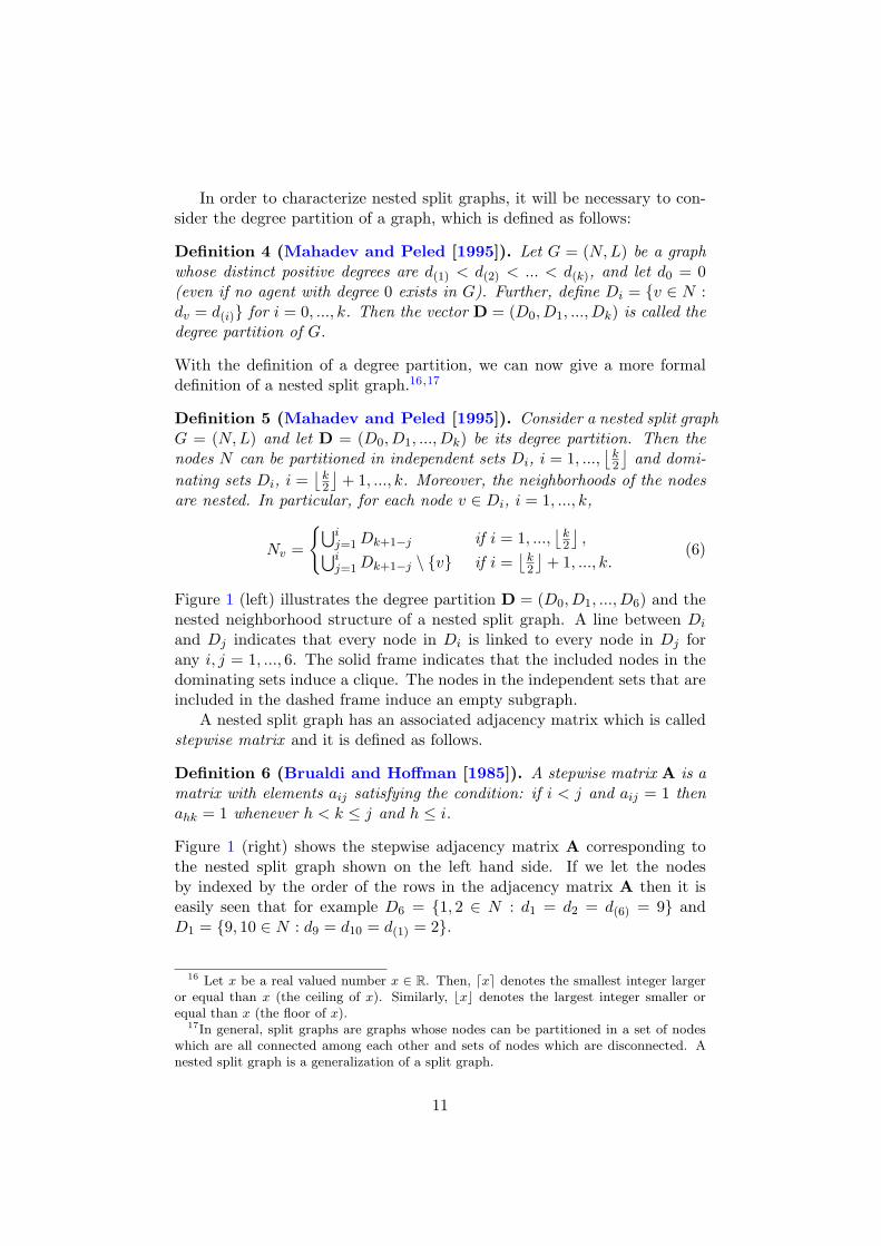
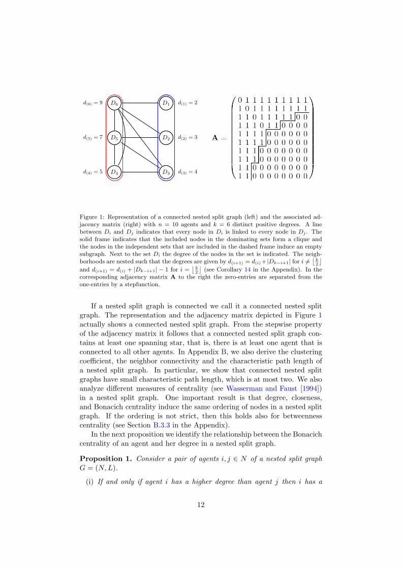
Figure 1 (left) illustrates the degree partition D = (D0, D1, ..., D6) and thenested neighborhood structure of a nested split graph. A line between Di
and Dj indicates that every node in Di is linked to every node in Dj forany i, j = 1, ..., 6. The solid frame indicates that the included nodes in thedominating sets induce a clique. The nodes in the independent sets that areincluded in the dashed frame induce an empty subgraph.
A nested split graph has an associated adjacency matrix which is calledstepwise matrix and it is defined as follows.
Definition 6 (Brualdi and Hoffman [1985]). A stepwise matrix A is amatrix with elements aij satisfying the condition: if i < j and aij = 1 thenahk = 1 whenever h < k ≤ j and h ≤ i.
Figure 1 (right) shows the stepwise adjacency matrix A corresponding tothe nested split graph shown on the left hand side. If we let the nodesby indexed by the order of the rows in the adjacency matrix A then it iseasily seen that for example D6 = 1, 2 ∈ N : d1 = d2 = d(6) = 9 andD1 = 9, 10 ∈ N : d9 = d10 = d(1) = 2.
16 Let x be a real valued number x ∈ R. Then, ⌈x⌉ denotes the smallest integer largeror equal than x (the ceiling of x). Similarly, ⌊x⌋ denotes the largest integer smaller orequal than x (the floor of x).
17In general, split graphs are graphs whose nodes can be partitioned in a set of nodeswhich are all connected among each other and sets of nodes which are disconnected. Anested split graph is a generalization of a split graph.
11
D1
D2
D3D4
D5
D6 D1 d(1) = 2
D2 d(2) = 3
D3 d(3) = 4D4d(4) = 5
D5d(5) = 7
D6d(6) = 9
Figure 1: Representation of a connected nested split graph (left) and the associated ad-jacency matrix (right) with n = 10 agents and k = 6 distinct positive degrees. A linebetween Di and Dj indicates that every node in Di is linked to every node in Dj . Thesolid frame indicates that the included nodes in the dominating sets form a clique andthe nodes in the independent sets that are included in the dashed frame induce an emptysubgraph. Next to the set Di the degree of the nodes in the set is indicated. The neigh-borhoods are nested such that the degrees are given by d(i+1) = d(i)+ |Dk−i+1| for i 6=
⌊
k2
⌋
and d(i+1) = d(i) + |Dk−i+1| − 1 for i =⌊
k2
⌋
(see Corollary 14 in the Appendix). In thecorresponding adjacency matrix A to the right the zero-entries are separated from theone-entries by a stepfunction.
If a nested split graph is connected we call it a connected nested splitgraph. The representation and the adjacency matrix depicted in Figure 1actually shows a connected nested split graph. From the stepwise propertyof the adjacency matrix it follows that a connected nested split graph con-tains at least one spanning star, that is, there is at least one agent that isconnected to all other agents. In Appendix B, we also derive the clusteringcoefficient, the neighbor connectivity and the characteristic path length ofa nested split graph. In particular, we show that connected nested splitgraphs have small characteristic path length, which is at most two. We alsoanalyze different measures of centrality (see Wasserman and Faust [1994])in a nested split graph. One important result is that degree, closeness,and Bonacich centrality induce the same ordering of nodes in a nested splitgraph. If the ordering is not strict, then this holds also for betweennesscentrality (see Section B.3.3 in the Appendix).
In the next proposition we identify the relationship between the Bonacichcentrality of an agent and her degree in a nested split graph.
Proposition 1. Consider a pair of agents i, j ∈ N of a nested split graphG = (N, L).
(i) If and only if agent i has a higher degree than agent j then i has a
12
higher Bonacich centrality than j, i.e.
di > dj ⇔ bi(G, λ) > bj(G, λ).
(ii) Assume that neither the links ik nor ij are in G, ij /∈ L and ik /∈ L.Further assume that agent k has a higher degree than agent j, dk > dj.Then adding the link ik to G increases the Bonacich centrality of agenti more than adding the link ij to G, i.e.
dk > dj ⇔ bi(G + ik, λ) > bi(G + ij, λ).
From part (ii) of Proposition 1 we find that when agent i has to decide tocreate a link either to agents k or j, with dk > dj , in the link formationprocess (G(t))∞t=0 then i will always connect to agent k because this linkgives i a higher Bonacich than the other link to agent j. We can make useof this property in order to show that the networks emerging from the linkformation process defined in the previous section actually are nested splitgraphs. This result is stated in the next proposition.
Proposition 2. Consider the network formation process (G(t))∞t=0 intro-duced in Definition 3. Then, at any time t, a network G(t) generated by(G(t))∞t=0 is a nested split graph.
This result is due to the fact that agents, when they have the possibilityof creating a new link, always connect to the agent who has the highestBonacich centrality (and by Proposition 1 the highest degree) among hersecond-order neighbors. This creates a nested neighborhood structure whichcan always be represented by a stepwise adjacency matrix after a possiblerelabeling of the agents.18 The same applies for link removal.
From the fact that G(t) is a nested split graph with an associated step-wise adjacency matrix it further follows that at any time t in the networkevolution, G(t) consists of a single connected component and possibly iso-lated agents.
Corollary 1. The network G(t), t = 0, 1, 2, ... generated by the network for-mation process (G(t))∞t=0 introduced in Definition 3 consists of one connectedcomponent and possibly isolated agents.
Nested split graphs are not only prominent in the literature on spectral graphtheory [Cvetkovic et al., 1997] but they have also appeared in the recent lit-erature on economic networks. Nested split graphs are so called “inter-linked
18Two graphs G = (N, L) and G′ = (N ′, L′) are the same unlabeled graph when theyare isomorphic, i.e., when there exists a permutation π of N such that ij ∈ L if and onlyif π(i)π(j) ∈ L′. Two states x, y ∈ Ω of the Markov process (G(t))∞
t=0 are identical, x = y,if they correspond to the same unlabeled graph.
13
stars” found in Goyal and Joshi [2003].19 Subsequently, Goyal et al. [2006]identified inter-linked stars in the network of scientific collaborations amongeconomists. It is important to note that nested split graphs are characterizedby a distinctive core-periphery structure. Core-periphery structures havebeen found in several empirical studies of interfirm collaborations networks[Baker et al., 2008; Gulati and Gargiulo, 1999]. The wider applicability ofnested split graphs suggests that a network formation process that gener-ates these graphs as it is defined in Definition 3 are of general relevance forunderstanding economic and social networks.
3. Stationary Networks: Characterization
In this section we show that the network formation process (G(t))∞t=0
defined in the previous section induces an ergodic Markov chain and we an-alyze the asymptotic states of this process as the number of agents becomeslarge. In particular, we can give the following proposition.
Proposition 3. The network formation process (G(t))∞t=0 introduced in Def-inition 3 induces an ergodic Markov chain on the state space Ω with a uniquestationary distribution µ. In particular, the state space Ω is finite and con-sists of all possible unlabeled nested split graphs on n nodes where the numberof possible states is given by |Ω| = 2n−1.
The symmetry of the network formation process (G(t))∞t=0 with respect tothe link formation probability α and the link removal probability 1−α allowsus to state the following proposition.
Proposition 4. Consider the network formation process (G(t))∞t=0 with linkcreation probability α and the network formation process (G′(t))∞t=0 with linkcreation probability 1 − α. Let µ be the stationary distribution of (G(t))∞t=0
and µ′ the stationary distribution of (G′(t))∞t=0. Then for each network G inthe stationary distribution µ with probability µG the complement of G, G,has the same probability µG in µ′, i.e. µ′
G= µG.
Proposition 4 allows us to derive the stationary distribution for any valueof 1/2 ≤ α ≤ 1 if we know the corresponding distribution for 1 − α. Thisfollows from the fact that the complement G of a nested split graph G isa nested split graph as well [Mahadev and Peled, 1995]. In particular, thenetworks G are nested split graphs in which the number of nodes in thedominating sets corresponds to the number of nodes in the independent sets
19Nested split graphs are inter-linked stars but an inter-linked star is not necessarilya nested split graph. Nested split graphs have a nested neighborhood structure for alldegrees while in an inter-linked star this holds only for the nodes with the lowest andhighest degrees.
14
in G and, conversely, the number of nodes in the independent sets in Gcorresponds to the number of nodes in the dominating sets in G.
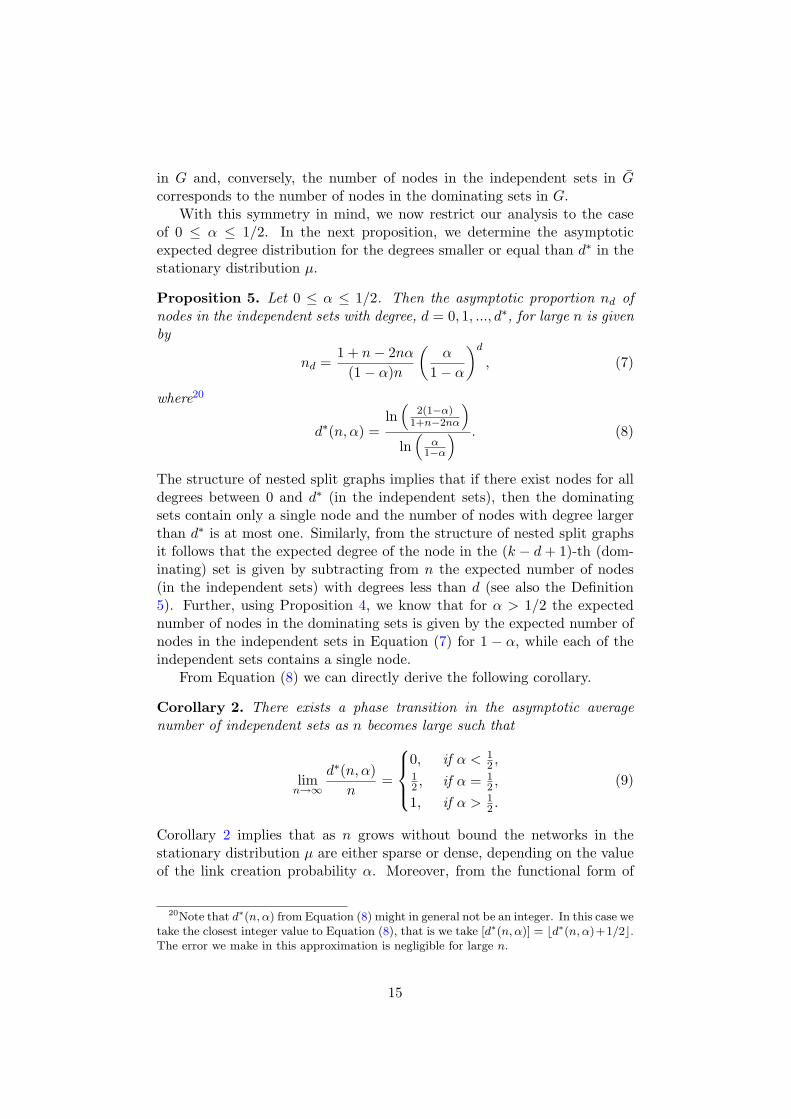
With this symmetry in mind, we now restrict our analysis to the caseof 0 ≤ α ≤ 1/2. In the next proposition, we determine the asymptoticexpected degree distribution for the degrees smaller or equal than d∗ in thestationary distribution µ.
Proposition 5. Let 0 ≤ α ≤ 1/2. Then the asymptotic proportion nd ofnodes in the independent sets with degree, d = 0, 1, ..., d∗, for large n is givenby
nd =1 + n − 2nα
(1 − α)n
(
α
1 − α
)d
, (7)
where20
d∗(n, α) =ln(
2(1−α)1+n−2nα
)
ln(
α1−α
) . (8)
The structure of nested split graphs implies that if there exist nodes for alldegrees between 0 and d∗ (in the independent sets), then the dominatingsets contain only a single node and the number of nodes with degree largerthan d∗ is at most one. Similarly, from the structure of nested split graphsit follows that the expected degree of the node in the (k − d + 1)-th (dom-inating) set is given by subtracting from n the expected number of nodes(in the independent sets) with degrees less than d (see also the Definition5). Further, using Proposition 4, we know that for α > 1/2 the expectednumber of nodes in the dominating sets is given by the expected number ofnodes in the independent sets in Equation (7) for 1 − α, while each of theindependent sets contains a single node.
From Equation (8) we can directly derive the following corollary.
Corollary 2. There exists a phase transition in the asymptotic averagenumber of independent sets as n becomes large such that
limn→∞
d∗(n, α)
n=
0, if α < 12 ,
12 , if α = 1
2 ,
1, if α > 12 .
(9)
Corollary 2 implies that as n grows without bound the networks in thestationary distribution µ are either sparse or dense, depending on the valueof the link creation probability α. Moreover, from the functional form of
20Note that d∗(n, α) from Equation (8) might in general not be an integer. In this case wetake the closest integer value to Equation (8), that is we take [d∗(n, α)] = ⌊d∗(n, α)+1/2⌋.The error we make in this approximation is negligible for large n.
15
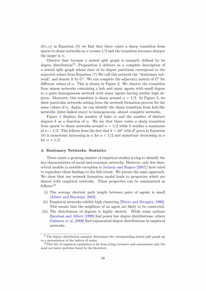
d(n, α) in Equation (8) we find that there exists a sharp transition fromsparse to dense networks as α crosses 1/2 and the transition becomes sharperthe larger is n.
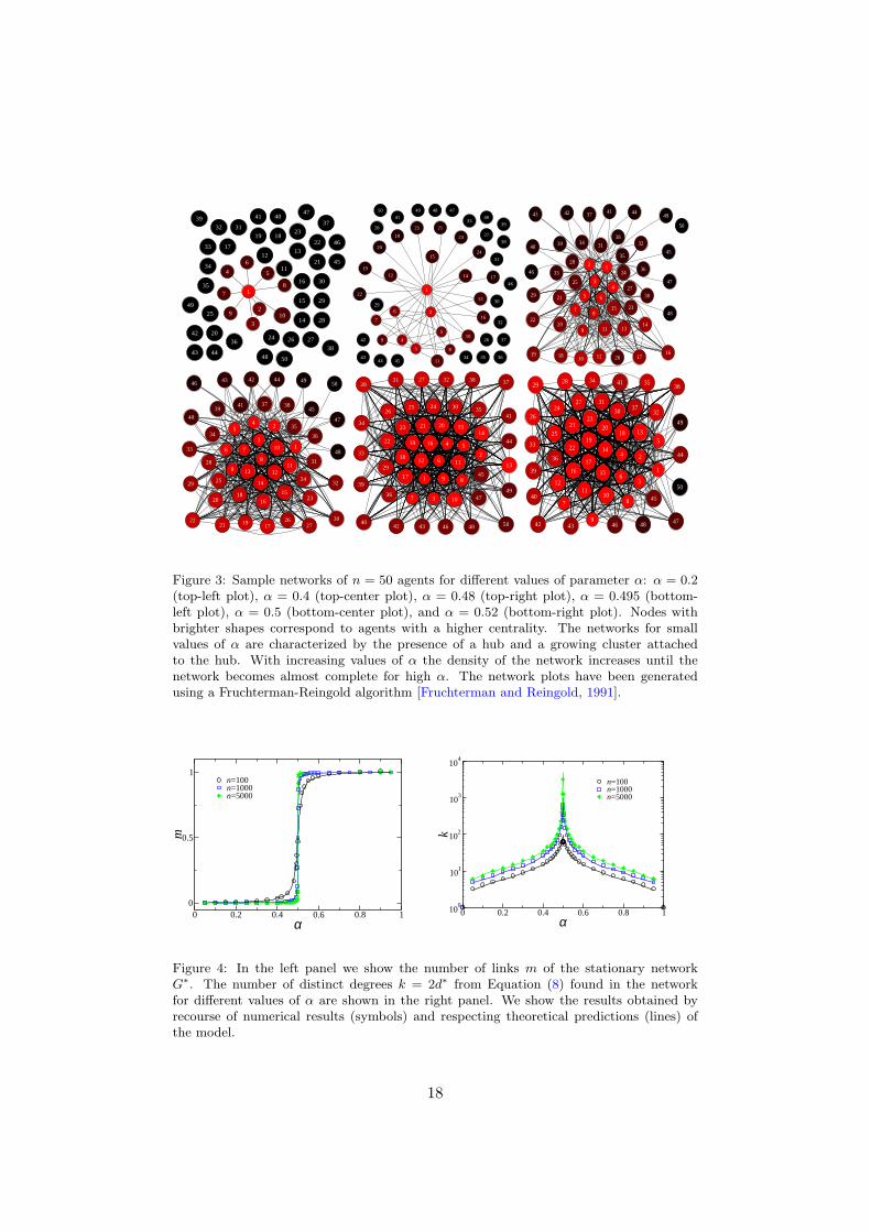
Observe that because a nested split graph is uniquely defined by itsdegree distribution21, Proposition 5 delivers us a complete description ofa nested split graph whose sizes of its degree partitions correspond to theexpected values from Equation (7).We call this network the “stationary net-work” and denote it by G∗. We can compute the adjacency matrix of G∗ fordifferent values of α. This is shown in Figure 2. We observe the transitionfrom sparse networks containing a hub and many agents with small degreeto a quite homogeneous network with many agents having similar high de-grees. Moreover, this transition is sharp around α = 1/2. In Figure 3, weshow particular networks arising from the network formation process for thesame values of α. Again, we can identify the sharp transition from hub-likenetworks (inter-linked stars) to homogeneous, almost complete networks.
Figure 4 displays the number of links m and the number of distinctdegrees k as a function of α. We see that there exists a sharp transitionfrom sparse to dense networks around α = 1/2 while k reaches a maximumat α = 1/2. This follows from the fact that k = 2d∗ with d∗ given in Equation(8) is monotonic increasing in α for α < 1/2 and monotonic decreasing in αfor α > 1/2.
4. Stationary Networks: Statistics
There exists a growing number of empirical studies trying to identify thekey characteristics of social and economic networks. However, only few theo-retical models (a notable exception is Jackson and Rogers [2007]) have triedto reproduce these findings to the full extent. We pursue the same approach.We show that our network formation model leads to properties which areshared with empirical networks. These properties can be summarized asfollows:22
(i) The average shortest path length between pairs of agents is small[Albert and Barabasi, 2002].
(ii) Empirical networks exhibit high clustering [Watts and Strogatz, 1998].This means that the neighbors of an agent are likely to be connected.
(iii) The distribution of degrees is highly skewed. While some authorsBarabasi and Albert [1999] find power law degree distributions, othersGuimera et al. [2006] find exponential degree distributions in empiricalnetworks.
21The degree distribution uniquely determines the corresponding nested split graph upto a permutation of the indices of nodes.
22This list of empirical regularities is far from being extensive and summarizes only themost pervasive patterns found in the literature.
16
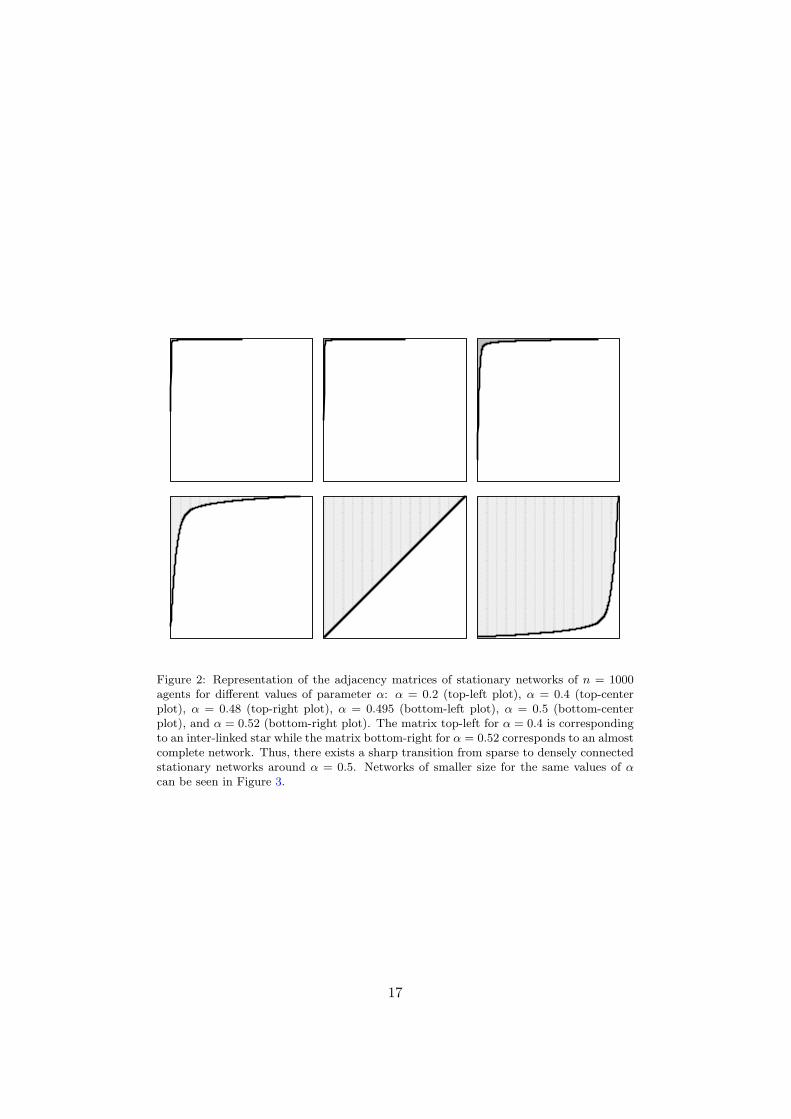
Figure 2: Representation of the adjacency matrices of stationary networks of n = 1000agents for different values of parameter α: α = 0.2 (top-left plot), α = 0.4 (top-centerplot), α = 0.48 (top-right plot), α = 0.495 (bottom-left plot), α = 0.5 (bottom-centerplot), and α = 0.52 (bottom-right plot). The matrix top-left for α = 0.4 is correspondingto an inter-linked star while the matrix bottom-right for α = 0.52 corresponds to an almostcomplete network. Thus, there exists a sharp transition from sparse to densely connectedstationary networks around α = 0.5. Networks of smaller size for the same values of αcan be seen in Figure 3.
17
1
2
3
4 5
6
78
9 10
11
1213
14
15
16
17
1819
20
21
22
23
24
25
26 27
28
29
30
3132
33
34
35
36
37
38
39 4041
42
43 44
45
46
47
48
49
50
1
2
3
4
5
6
7
8
910
11
12
13
14
15
16
17
18
19
20
21
22
23
24
25
26
27
28
2930
31
32
33
34 35 36
37
38
39
4041
42
4344 45
46
47484950
12
34
5 6
78
9
10
11
12
1314
15
16171819
20
21
22
23
24
25
26
27
28
29 30
31 32
33
34
35
36
37
383940
414243 44
45
46
47
48
49
50
1
2
3
45
6 7
8
9
10
111213
14
15
16
17
18
19
20
2122
23
2425
2627
28
29
30
31
32
33
3435
36
37 3839
40
41
4243 44
45
46
47
48
4950
1
2
3
4 5
6
7
89
10
111213
1415
16
17
18
19
2021
22
23
242526
2728
29
30
31 32
33
34
35
36
3738
39
40
41
42 43
44
45
46
47
48
49
50
1
2
3
4
5
6
7 8
9
1011
12
13
14
151617
1819
2021
22
23
24
25
26
27
2829
30
31
32
33
34 35
36
37
38
39
40
41
42 43
44
45
46 4748
49
50
Figure 3: Sample networks of n = 50 agents for different values of parameter α: α = 0.2(top-left plot), α = 0.4 (top-center plot), α = 0.48 (top-right plot), α = 0.495 (bottom-left plot), α = 0.5 (bottom-center plot), and α = 0.52 (bottom-right plot). Nodes withbrighter shapes correspond to agents with a higher centrality. The networks for smallvalues of α are characterized by the presence of a hub and a growing cluster attachedto the hub. With increasing values of α the density of the network increases until thenetwork becomes almost complete for high α. The network plots have been generatedusing a Fruchterman-Reingold algorithm [Fruchterman and Reingold, 1991].
0 0.2 0.4 0.6 0.8 1α
0
0.5
1
m
n=100n=1000n=5000
0 0.2 0.4 0.6 0.8 1α
100
101
102
103
104
k
n=100n=1000n=5000
Figure 4: In the left panel we show the number of links m of the stationary networkG∗. The number of distinct degrees k = 2d∗ from Equation (8) found in the networkfor different values of α are shown in the right panel. We show the results obtained byrecourse of numerical results (symbols) and respecting theoretical predictions (lines) ofthe model.
18
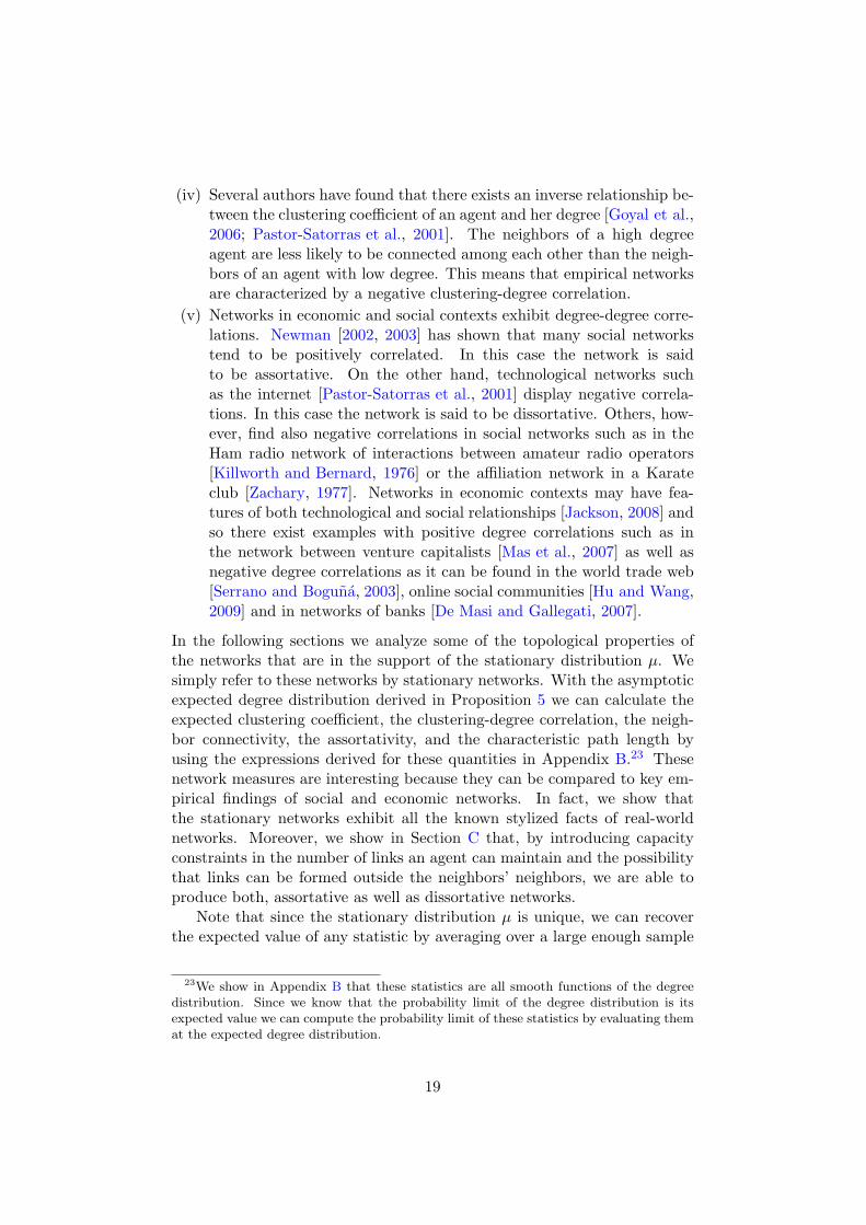
(iv) Several authors have found that there exists an inverse relationship be-tween the clustering coefficient of an agent and her degree [Goyal et al.,2006; Pastor-Satorras et al., 2001]. The neighbors of a high degreeagent are less likely to be connected among each other than the neigh-bors of an agent with low degree. This means that empirical networksare characterized by a negative clustering-degree correlation.
(v) Networks in economic and social contexts exhibit degree-degree corre-lations. Newman [2002, 2003] has shown that many social networkstend to be positively correlated. In this case the network is saidto be assortative. On the other hand, technological networks suchas the internet [Pastor-Satorras et al., 2001] display negative correla-tions. In this case the network is said to be dissortative. Others, how-ever, find also negative correlations in social networks such as in theHam radio network of interactions between amateur radio operators[Killworth and Bernard, 1976] or the affiliation network in a Karateclub [Zachary, 1977]. Networks in economic contexts may have fea-tures of both technological and social relationships [Jackson, 2008] andso there exist examples with positive degree correlations such as inthe network between venture capitalists [Mas et al., 2007] as well asnegative degree correlations as it can be found in the world trade web[Serrano and Boguna, 2003], online social communities [Hu and Wang,2009] and in networks of banks [De Masi and Gallegati, 2007].
In the following sections we analyze some of the topological properties ofthe networks that are in the support of the stationary distribution µ. Wesimply refer to these networks by stationary networks. With the asymptoticexpected degree distribution derived in Proposition 5 we can calculate theexpected clustering coefficient, the clustering-degree correlation, the neigh-bor connectivity, the assortativity, and the characteristic path length byusing the expressions derived for these quantities in Appendix B.23 Thesenetwork measures are interesting because they can be compared to key em-pirical findings of social and economic networks. In fact, we show thatthe stationary networks exhibit all the known stylized facts of real-worldnetworks. Moreover, we show in Section C that, by introducing capacityconstraints in the number of links an agent can maintain and the possibilitythat links can be formed outside the neighbors’ neighbors, we are able toproduce both, assortative as well as dissortative networks.
Note that since the stationary distribution µ is unique, we can recoverthe expected value of any statistic by averaging over a large enough sample
23We show in Appendix B that these statistics are all smooth functions of the degreedistribution. Since we know that the probability limit of the degree distribution is itsexpected value we can compute the probability limit of these statistics by evaluating themat the expected degree distribution.
19
of empirical networks generated by numerical simulations. We then super-impose the analytical predictions of the statistic derived from Proposition 5with the sample averages in order to compare the validity of our theoreticalresults, also for small network sizes n. As we will show, there is a goodagreement of the theory with the empirical results for all system sizes.
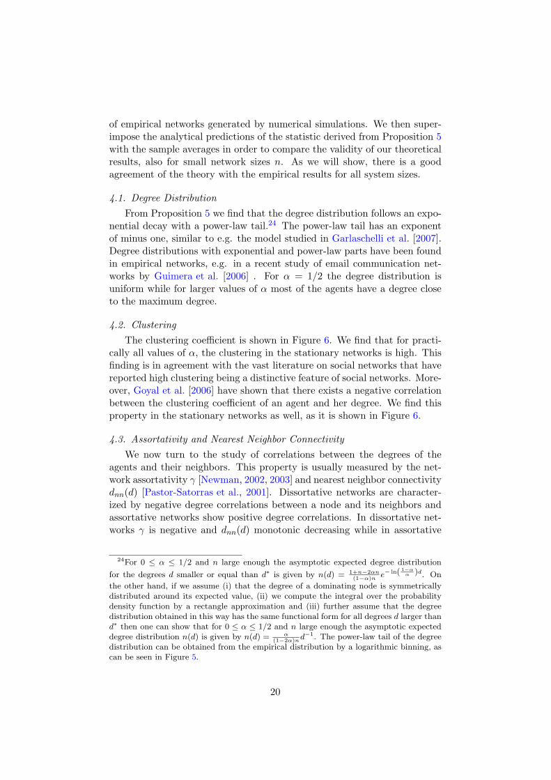
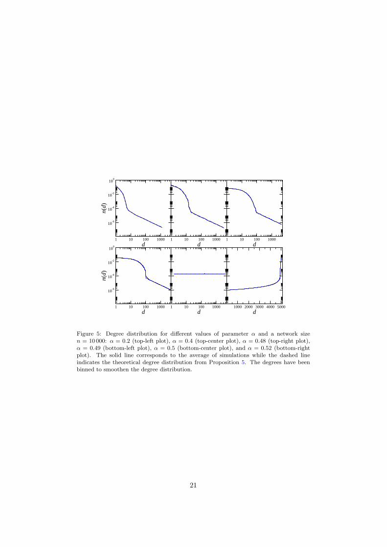
4.1. Degree Distribution
From Proposition 5 we find that the degree distribution follows an expo-nential decay with a power-law tail.24 The power-law tail has an exponentof minus one, similar to e.g. the model studied in Garlaschelli et al. [2007].Degree distributions with exponential and power-law parts have been foundin empirical networks, e.g. in a recent study of email communication net-works by Guimera et al. [2006] . For α = 1/2 the degree distribution isuniform while for larger values of α most of the agents have a degree closeto the maximum degree.
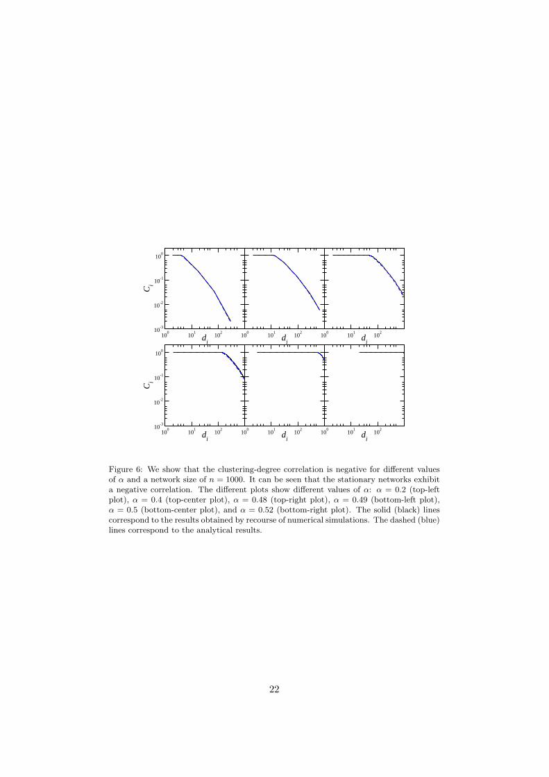
4.2. Clustering
The clustering coefficient is shown in Figure 6. We find that for practi-cally all values of α, the clustering in the stationary networks is high. Thisfinding is in agreement with the vast literature on social networks that havereported high clustering being a distinctive feature of social networks. More-over, Goyal et al. [2006] have shown that there exists a negative correlationbetween the clustering coefficient of an agent and her degree. We find thisproperty in the stationary networks as well, as it is shown in Figure 6.
4.3. Assortativity and Nearest Neighbor Connectivity
We now turn to the study of correlations between the degrees of theagents and their neighbors. This property is usually measured by the net-work assortativity γ [Newman, 2002, 2003] and nearest neighbor connectivitydnn(d) [Pastor-Satorras et al., 2001]. Dissortative networks are character-ized by negative degree correlations between a node and its neighbors andassortative networks show positive degree correlations. In dissortative net-works γ is negative and dnn(d) monotonic decreasing while in assortative
24For 0 ≤ α ≤ 1/2 and n large enough the asymptotic expected degree distribution
for the degrees d smaller or equal than d∗ is given by n(d) = 1+n−2αn(1−α)n
e− ln( 1−αα )d. On
the other hand, if we assume (i) that the degree of a dominating node is symmetricallydistributed around its expected value, (ii) we compute the integral over the probabilitydensity function by a rectangle approximation and (iii) further assume that the degreedistribution obtained in this way has the same functional form for all degrees d larger thand∗ then one can show that for 0 ≤ α ≤ 1/2 and n large enough the asymptotic expecteddegree distribution n(d) is given by n(d) = α
(1−2α)nd−1. The power-law tail of the degree
distribution can be obtained from the empirical distribution by a logarithmic binning, ascan be seen in Figure 5.
20
1 10 100 1000d
10-6
10-4
10-2
100
n(d)
1 10 100 1000d
1 10 100 1000d
1 10 100 1000d
10-6
10-4
10-2
100
n(d)
1 10 100 1000d
1000 2000 3000 4000 5000d
Figure 5: Degree distribution for different values of parameter α and a network sizen = 10 000: α = 0.2 (top-left plot), α = 0.4 (top-center plot), α = 0.48 (top-right plot),α = 0.49 (bottom-left plot), α = 0.5 (bottom-center plot), and α = 0.52 (bottom-rightplot). The solid line corresponds to the average of simulations while the dashed lineindicates the theoretical degree distribution from Proposition 5. The degrees have beenbinned to smoothen the degree distribution.
21
100
101
102
di
10-3
10-2
10-1
100
Ci
100
101
102
di
100
101
102
di
100
101
102
di
10-3
10-2
10-1
100
Ci
100
101
102
di
100
101
102
di
Figure 6: We show that the clustering-degree correlation is negative for different valuesof α and a network size of n = 1000. It can be seen that the stationary networks exhibita negative correlation. The different plots show different values of α: α = 0.2 (top-leftplot), α = 0.4 (top-center plot), α = 0.48 (top-right plot), α = 0.49 (bottom-left plot),α = 0.5 (bottom-center plot), and α = 0.52 (bottom-right plot). The solid (black) linescorrespond to the results obtained by recourse of numerical simulations. The dashed (blue)lines correspond to the analytical results.
22
0 0.2 0.4 0.6 0.8 1
α-1
-0.8
-0.6
-0.4
-0.2
0
0.2
γ
n=100n=1000n=5000
100
101
102
103
104
d
100
101
102
103
<d nm
>
100
101
102
d10
010
110
2
d
100
101
102
d
101
102
103
<d nm
>
100
101
102
d10
010
110
2
d
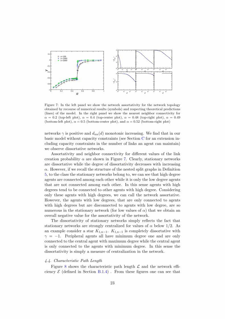
Figure 7: In the left panel we show the network assortativity for the network topologyobtained by recourse of numerical results (symbols) and respecting theoretical predictions(lines) of the model. In the right panel we show the nearest neighbor connectivity forα = 0.2 (top-left plot), α = 0.4 (top-center plot), α = 0.48 (top-right plot), α = 0.49(bottom-left plot), α = 0.5 (bottom-center plot), and α = 0.52 (bottom-right plot)
networks γ is positive and dnn(d) monotonic increasing. We find that in ourbasic model without capacity constraints (see Section C for an extension in-cluding capacity constraints in the number of links an agent can maintain)we observe dissortative networks.
Assortativity and neighbor connectivity for different values of the linkcreation probability α are shown in Figure 7. Clearly, stationary networksare dissortative while the degree of dissortativity decreases with increasingα. However, if we recall the structure of the nested split graphs in Definition5, to the class the stationary networks belong to, we can see that high degreeagents are connected among each other while it is only the low degree agentsthat are not connected among each other. In this sense agents with highdegrees tend to be connected to other agents with high degree. Consideringonly these agents with high degrees, we can call the network assortative.However, the agents with low degrees, that are only connected to agentswith high degrees but are disconnected to agents with low degree, are sonumerous in the stationary network (for low values of α) that we obtain anoverall negative value for the assortativity of the network.
The dissortativity of stationary networks simply reflects the fact thatstationary networks are strongly centralized for values of α below 1/2. Asan example consider a star K1,n−1. K1,n−1 is completely dissortative withγ = −1. Peripheral agents all have minimum degree one and are onlyconnected to the central agent with maximum degree while the central agentis only connected to the agents with minimum degree. In this sense thedissortativity is simply a measure of centralization in the network.
4.4. Characteristic Path Length
Figure 8 shows the characteristic path length L and the network effi-ciency E (defined in Section B.1.4) . From these figures one can see that
23
0 0.2 0.4 0.6 0.8 1
α
1
1.5
2
L
n=100n=1000n=5000
0 0.2 0.4 0.6 0.8 1
α0
0.5
1
ε
n=100n=1000n=5000
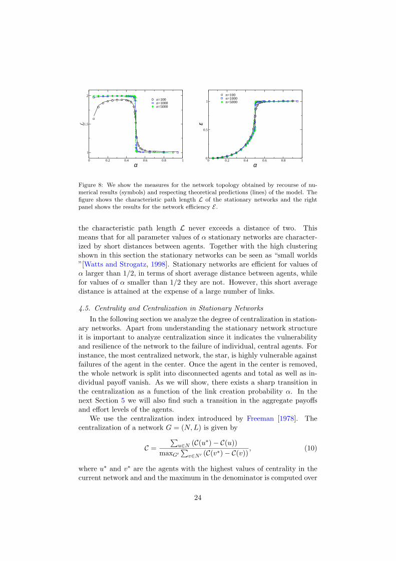
Figure 8: We show the measures for the network topology obtained by recourse of nu-merical results (symbols) and respecting theoretical predictions (lines) of the model. Thefigure shows the characteristic path length L of the stationary networks and the rightpanel shows the results for the network efficiency E .
the characteristic path length L never exceeds a distance of two. Thismeans that for all parameter values of α stationary networks are character-ized by short distances between agents. Together with the high clusteringshown in this section the stationary networks can be seen as “small worlds”[Watts and Strogatz, 1998]. Stationary networks are efficient for values ofα larger than 1/2, in terms of short average distance between agents, whilefor values of α smaller than 1/2 they are not. However, this short averagedistance is attained at the expense of a large number of links.
4.5. Centrality and Centralization in Stationary Networks
In the following section we analyze the degree of centralization in station-ary networks. Apart from understanding the stationary network structureit is important to analyze centralization since it indicates the vulnerabilityand resilience of the network to the failure of individual, central agents. Forinstance, the most centralized network, the star, is highly vulnerable againstfailures of the agent in the center. Once the agent in the center is removed,the whole network is split into disconnected agents and total as well as in-dividual payoff vanish. As we will show, there exists a sharp transition inthe centralization as a function of the link creation probability α. In thenext Section 5 we will also find such a transition in the aggregate payoffsand effort levels of the agents.
We use the centralization index introduced by Freeman [1978]. Thecentralization of a network G = (N, L) is given by
C =
∑
u∈N (C(u∗) − C(u))
maxG′
∑
v∈N ′ (C(v∗) − C(v)), (10)
where u∗ and v∗ are the agents with the highest values of centrality in thecurrent network and and the maximum in the denominator is computed over
24
0 0.2 0.4 0.6 0.8 1
α
0
0.2
0.4
0.6
0.8
1
Cd
n=100n=1000n=5000
0 0.2 0.4 0.6 0.8 1
α
0
0.2
0.4
0.6
0.8
1
Cc
n=100n=1000n=5000
0 0.2 0.4 0.6 0.8 1
α
0
0.2
0.4
0.6
0.8
1
Cb
n=100n=1000n=5000
0 0.2 0.4 0.6 0.8 1
α
0
0.2
0.4
0.6
0.8
1
Cv
n=100n=1000n=5000
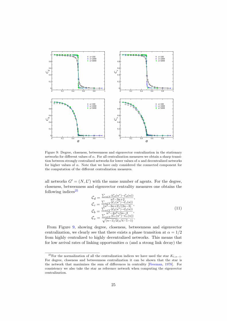
Figure 9: Degree, closeness, betweenness and eigenvector centralization in the stationarynetworks for different values of α. For all centralization measures we obtain a sharp transi-tion between strongly centralized networks for lower values of α and decentralized networksfor higher values of α. Note that we have only considered the connected component forthe computation of the different centralization measures.
all networks G′ = (N, L′) with the same number of agents. For the degree,closeness, betweenness and eigenvector centrality measures one obtains thefollowing indices25
Cd =∑
u∈V (Cd(u∗)−Cd(u))
n2−3n+2,
Cc =∑
u∈V (Cc(u∗)−Cc(u))
(n2−3n+2)/(2n−3),
Cb =∑
u∈V (Cb(u∗)−Cb(u))
n3−4n2+5n−2,
Cv =∑
u∈V (Cv(u∗)−Cv(u))√(n−1)/2(
√n−1−1)
.
(11)
From Figure 9, showing degree, closeness, betweenness and eigenvectorcentralization, we clearly see that there exists a phase transition at α = 1/2from highly centralized to highly decentralized networks. This means thatfor low arrival rates of linking opportunities α (and a strong link decay) the
25For the normalization of all the centralization indices we have used the star K1,n−1.For degree, closeness and betweenness centralization it can be shown that the star isthe network that maximizes the sum of differences in centrality [Freeman, 1978]. Forconsistency we also take the star as reference network when computing the eigenvectorcentralization.
25
stationary network is strongly polarized, composed mainly of a star (or aninter-linked star as in Goyal and Joshi [2003]), while for high arrival ratesof linking opportunities (and a weak link decay) stationary networks arelargely homogeneous. We can also see that the transition between thesestates is sharp.
Our findings are in line with previous works studying the optimal inter-nal communication structure of organizations [Guimera et al., 2002]. Otherworks [Calvo-Armengol and Martı, 2009; Dodds et al., 2003; Dupouet and Yildizoglu,2006; Huberman and Hogg, 1995] have discussed the conditions under whichinformal organizational networks outperform centralized structures in com-plex, changing environments and under which conditions hierarchies aremore efficient. Similar to Arenas et al. [2008] and Ehrhardt et al. [2006a],we find sharp transitions between largely homogeneous and centralized net-works. Moreover, the stationary networks in our model are polarized andstrongly centralized for a low volatility in the environment associated withmany linking opportunities whereas they are homogeneous and largely de-centralized for a highly volatile environment with few linking opportunitiesand a strong link decay. The hierarchical structure of stationary networksand its dependency on the volatility is similar to the findings for optimalnetworks in Arenas et al. [2008].
5. Stationary Networks: Efficiency
We now turn to the investigation of the optimality and efficiency of sta-tionary networks. Following Jackson [2008]; Jackson and Wolinsky [1996],we define social welfare as the sum of the agents’ individual payoffs
Π(x∗, G) =n∑
i=1
πi(x∗, G). (12)
We are interested in the solution of the following social planner’s problem.Let G(n) denote the set of connected graphs having n agents in total. Thesocial planner’s solution is given by
H = argmaxG∈G(n)
Π(x∗, G). (13)
A graph H solving the maximization problem in Equation (13) will be de-noted as “efficient”. The efficient network has been derived in Ballester et al.[2006] and we state their result in the following proposition.
Proposition 6 (Ballester et al. [2006]). Let G(n) denote the set of con-nected graphs having n agents and consider G ∈ G(n). Then the efficientnetwork H maximizing aggregate equilibrium contribution and payoff is thecomplete graph Kn.
26
This proposition is a direct consequence of Theorem 2 in Ballester et al.[2006] where more links is always better. Moreover, Corbo et al. [2006] haveshown that in the case of strong complementarities when λ approaches 1/λPF
maximizing aggregate equilibrium payoffs is equivalent to maximizing thelargest real eigenvalue λPF of the network.26
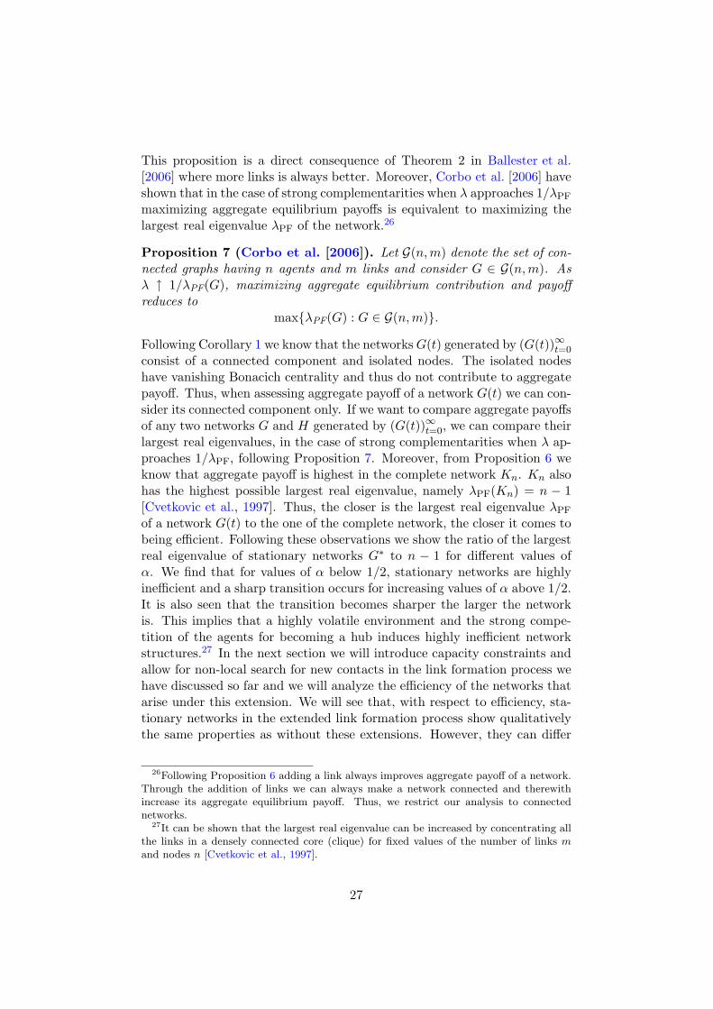
Proposition 7 (Corbo et al. [2006]). Let G(n, m) denote the set of con-nected graphs having n agents and m links and consider G ∈ G(n, m). Asλ ↑ 1/λPF(G), maximizing aggregate equilibrium contribution and payoffreduces to
maxλPF(G) : G ∈ G(n, m).
Following Corollary 1 we know that the networks G(t) generated by (G(t))∞t=0
consist of a connected component and isolated nodes. The isolated nodeshave vanishing Bonacich centrality and thus do not contribute to aggregatepayoff. Thus, when assessing aggregate payoff of a network G(t) we can con-sider its connected component only. If we want to compare aggregate payoffsof any two networks G and H generated by (G(t))∞t=0, we can compare theirlargest real eigenvalues, in the case of strong complementarities when λ ap-proaches 1/λPF, following Proposition 7. Moreover, from Proposition 6 weknow that aggregate payoff is highest in the complete network Kn. Kn alsohas the highest possible largest real eigenvalue, namely λPF(Kn) = n − 1[Cvetkovic et al., 1997]. Thus, the closer is the largest real eigenvalue λPF
of a network G(t) to the one of the complete network, the closer it comes tobeing efficient. Following these observations we show the ratio of the largestreal eigenvalue of stationary networks G∗ to n − 1 for different values ofα. We find that for values of α below 1/2, stationary networks are highlyinefficient and a sharp transition occurs for increasing values of α above 1/2.It is also seen that the transition becomes sharper the larger the networkis. This implies that a highly volatile environment and the strong compe-tition of the agents for becoming a hub induces highly inefficient networkstructures.27 In the next section we will introduce capacity constraints andallow for non-local search for new contacts in the link formation process wehave discussed so far and we will analyze the efficiency of the networks thatarise under this extension. We will see that, with respect to efficiency, sta-tionary networks in the extended link formation process show qualitativelythe same properties as without these extensions. However, they can differ
26Following Proposition 6 adding a link always improves aggregate payoff of a network.Through the addition of links we can always make a network connected and therewithincrease its aggregate equilibrium payoff. Thus, we restrict our analysis to connectednetworks.
27It can be shown that the largest real eigenvalue can be increased by concentrating allthe links in a densely connected core (clique) for fixed values of the number of links mand nodes n [Cvetkovic et al., 1997].
27
0 0.2 0.4 0.6 0.8 1
α
0
0.2
0.4
0.6
0.8
1
λ PF(G
* )/(n
-1)
n=100n=1000n=5000
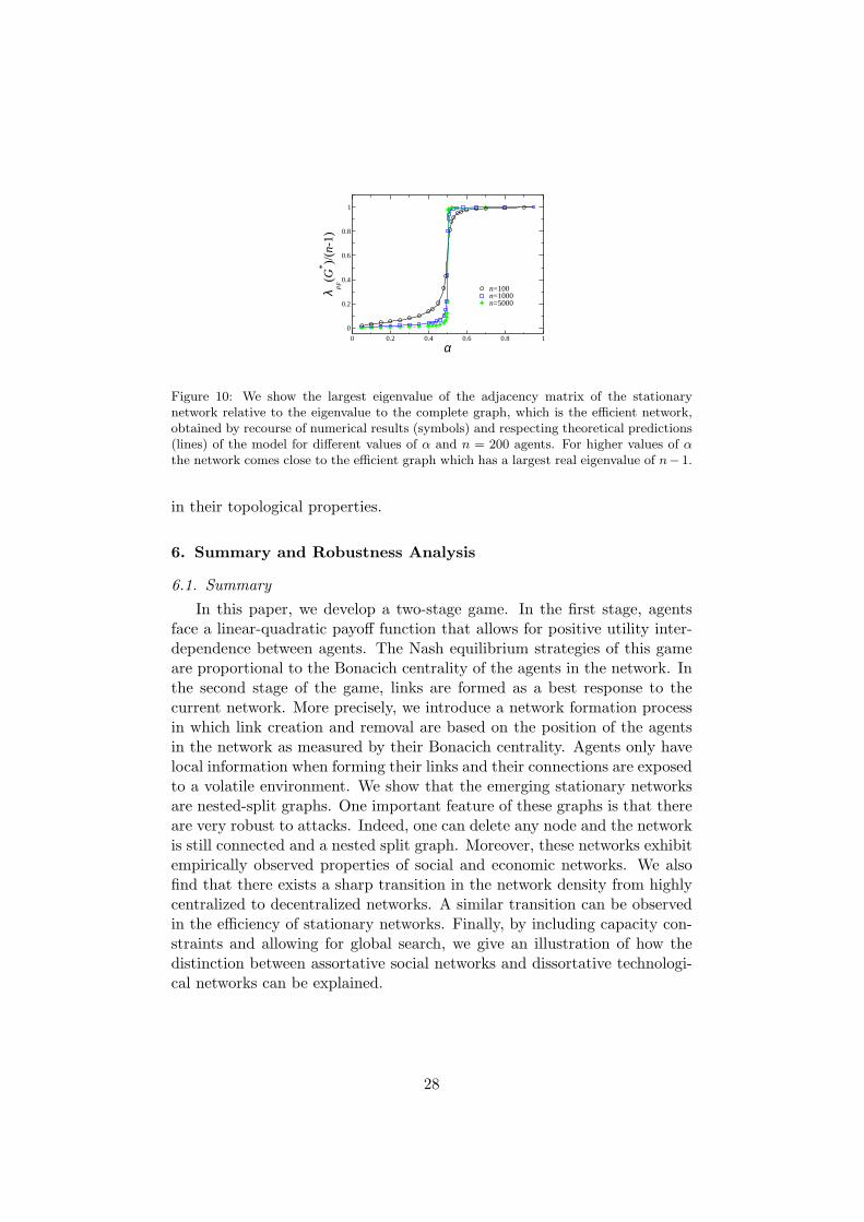
Figure 10: We show the largest eigenvalue of the adjacency matrix of the stationarynetwork relative to the eigenvalue to the complete graph, which is the efficient network,obtained by recourse of numerical results (symbols) and respecting theoretical predictions(lines) of the model for different values of α and n = 200 agents. For higher values of αthe network comes close to the efficient graph which has a largest real eigenvalue of n− 1.
in their topological properties.
6. Summary and Robustness Analysis
6.1. Summary
In this paper, we develop a two-stage game. In the first stage, agentsface a linear-quadratic payoff function that allows for positive utility inter-dependence between agents. The Nash equilibrium strategies of this gameare proportional to the Bonacich centrality of the agents in the network. Inthe second stage of the game, links are formed as a best response to thecurrent network. More precisely, we introduce a network formation processin which link creation and removal are based on the position of the agentsin the network as measured by their Bonacich centrality. Agents only havelocal information when forming their links and their connections are exposedto a volatile environment. We show that the emerging stationary networksare nested-split graphs. One important feature of these graphs is that thereare very robust to attacks. Indeed, one can delete any node and the networkis still connected and a nested split graph. Moreover, these networks exhibitempirically observed properties of social and economic networks. We alsofind that there exists a sharp transition in the network density from highlycentralized to decentralized networks. A similar transition can be observedin the efficiency of stationary networks. Finally, by including capacity con-straints and allowing for global search, we give an illustration of how thedistinction between assortative social networks and dissortative technologi-cal networks can be explained.
28
6.2. Robustness Analysis
We discuss different generalizations of our model. First, our analysisis restricted to linear-quadratic utility function (see Equation (1)), captur-ing linear externalities in players’ efforts. This leads to a Nash-equilibriumpayoff which is a function of the Bonacich centrality of each player (seeEquation (5)). For this equilibrium to be characterized, we also impose thatλ, the size of the interactions, has to be strictly lower than the inverse ofthe largest eigenvalue of the adjacency matrix of the network (see Theorem1). We can generalize our analysis as follows. Consider now a game whereplayers can only form or severe links but do not choose effort levels. In thatcase, if we use as payoffs Equation (5) or any increasing transformation ofthis payoff, then by considering the network formation process defined inDefinition 3, all our results will be the same without, however, relying onany specific form of the utility function. The only requirement is that theutility of each player is increasing in her Bonacich centrality. We can goeven further. Consider again the game where players do not choose efforts,then all our results will be valid if the utility function of each player is anincreasing function of her closeness centrality28 or given by the utility func-tion of the connection model of Jackson and Wolinsky [1996] when costs arezero.29 Furthermore, if the utility function of a player is increasing in thenumber of links of her direct neighbors or any centrality measure30 of herdirect neighbors (see Corollary 11), then all result are valid. Observe thatin all the cases when we do not use the Bonacich centrality in the utilityfunction, then not only we do not rely on any specific form of the utilityfunction but we do not even need the eigenvalue value condition mentionedabove.
Second, in our network-formation game defined in Definitions 2 and 3,we impose that, when forming a link (a) a player i needs to choose onlyamong her second-order neighbors, (b) player i has to be the best-responsefor the chosen second-order neighbor j. Because the networks that emergeare always nested-split graphs, these two assumptions turn out not to benecessary. Indeed, because of the specificity of nested-split graphs, wherethe maximum distance between players is 2, all the possible players arealready contained in the second-order neighbors.So assumption (a) is notnecessary. Also, when player i has the possibility to create a link with j, the
28Observe that for degree centrality, a player is indifferent between creating a link withanybody in the network, because it will increase her degree by one. In that case, we couldimpose some condition to guarantee that she will connect to the player with the highestdegree, and then our results will hold
29Observe that, in our model, there are indirect costs because when a player is chosenwith probability 1 − α, she is obliged to severe a link, which is costly.
30For betweenness centrality, we would need to impose some condition stating that,when indifferent, a player will always connect to the player with the highest degree
29
latter will always accept because it increases her payoff. In other words, idoes not need to be the best response for j to increase her payoff and, as aresult, (b) is not needed. It turns out, however, that in nested-split graphs,i is always the best response for j. This is a result of the network formationgame and not an assumption.
Third, in Section 4.1, for the nodes in the dominating sets, we obtain apower-law degree distribution with exponent minus one. We can extend ourmodel to obtain an arbitrary power law degree distribution by making theprobability of creating a link for player i, i.e. α, depending on, |Di|, the sizeof the degree partition she belongs to.
Finally, with our network formation game we always obtain negativedegree-degree correlation (i.e. our networks are dissortative). In AppendixC, we extend our game by including capacity constraints in the number oflinks an agent can maintain and a global search mechanism for new linkingpartners. We find that by introducing capacity constraints and global search,stationary networks can become assortative. Thus, we are able to repro-duce all topological properties of empirically observed social and economicnetworks. Moreover, the emergence of assortativity and positive degree-correlations respectively can be explained by considering limitations in thenumber of links an agent can maintain. This may be of particular relevancefor social networks and give an explanation for the distinction between as-sortative social networks and dissortative technological networks suggestedin Newman [2002].
References
Albert, R., Barabasi, A.-L., Jan 2002. Statistical mechanics of complex net-works. Rev. Mod. Phys. 74 (1), 47–97.
Aouchiche, M., Bell, F., Cvetkovic, D., Hansen, P., Rowlinson, P., Simic, S.,Stevanovic, D., 2006. Variable neighborhood search for extremal graphs,16. some conjectures related to the largest eigenvalue of a graph. Europ.J. Oper. Res.To appear.
Arenas, A., Cabrales, A., Dıaz-Guilera, A., Guimera, R., Vega-Redondo,F., 2008. Optimal information transmission in organizations: Search andcongestion. Review of Economic Design.
Baker, G., Gibbons, R., Murphy, K., 2008. Strategic Alliances: BridgesBetween “Islands of Conscious Power”? Journal of the Japanese andInternational Economies 22 (2), 146–163.
Bala, V., Goyal, S., 2000. A noncooperative model of network formation.Econometrica 68 (5), 1181–1230.
Ballester, C., Calvo-Armengol, A., Zenou, Y., 2006. Who’s who in networks.wanted: The key player. Econometrica 74 (5), 1403–1417.
Barabasi, A.-L., Albert, R., 1999. Emergence of scaling in random networks.Science 286, 509–512.
Bavelas, A., 1948. A mathematical model for group structures. Human Or-ganization 7, 16–30.
Beauchamp, M. A., 1965. An improved index of centrality. Behavioral Sci-ence 10, 161–163.
30
Bell, F., 1991. On the maximal index of connected graphs. Linear Algebraand its Applications 144, 135–151.
Benaim, M., Weibull, J., 2003. Deterministic approximation of stochasticevolution in games. Econometrica, 873–903.
Boje, D. M., Whetten, D. A., 1981. Effects of organizational strategies andcontextual constraints on centrality and attributions of influence in in-terorganizational networks. Administrative Science Quarterly 26 (March),378–395.
Bollobas, B., 1985. Random Graphs, 2nd Edition. Cambridge UniversityPress.
Bonacich, P., 1987. Power and centrality: A family of measures. AmericanJournal of Sociology 92 (5), 1170.
Bonacich, P., Lloyd, P., 2001. Eigenvector-like measures of centrality forasymmetric relations. Social Networks 23 (3), 191–201.
Borgatti, S., 2005. Centrality and network flow. Social Networks 27 (1),55–71.
Bramoulle, Y., Kranton, R., 2007. Public goods in networks. Journal ofEconomic Theory 135, 478–494.
Bramoulle, Y., Lopez-Pintado, D., Goyal, S., Vega-Redondo, F., 2004. So-cial interaction in anti-coordination games. International Journal of GameTheory 33, 1–20.
Brass, D. J., 1984. Being in the right place: A structural analysis of individ-ual influence in an organization. Administrative Science Quarterly 29 (4),518–539.
Brualdi, R. A., Hoffman, A. J., 1985. On the spectral radius of 0-1 matrices.Linear Algebra and Application 65, 133–146.
Cabrales, A., Calvo-Armengol, A., Zenou, Y., 2009. Social interactions andspillovers, Unpublished manuscript, Stockholm University.
Calvo-Armengol, A., de Martı, J., 2009. Information gathering in organiza-tions: Equilibrium, welfare and optimal network structure. Journal of theEuropean Economic Association 7, 116–161.
Calvo-Armengol, A., Patacchini, E., Zenou, Y., 2009. Peer effects and socialnetworks in education. Review of Economic Studies, forthcoming.
Calvo-Armengol, A., Zenou, Y., 2004. Social networks and crime decisions:The role of social structure in facilitating delinquent behavior. Interna-tional Economic Review 45 (3), 939–958.
Cook, K. S., Emerson, R. M., Gillmore, M. R., Yamagishi, T., 1983. Thedistribution of power in exchange networks: Theory and experimentalresults. The American Journal of Sociology 89 (2), 275–305.
Corbo, J., Calvo-Armengol, A., Parkes, D., 2006. A study of nash equilib-rium in contribution games for peer-to-peer networks. SIGOPS OperationSystems Review 40 (3), 61–66.
Cvetkovic, D., Rowlinson, P., Simic, S., 1997. Eigenspaces of Graphs.Vol. 66. Cambridge University Press, Encyclopedia of Mathematics.
Cvetkovic, D., Rowlinson, P., Simic, S. K., 2007. Eigenvalue bound for thesignless laplacian. Publications de l’institute mathematique, nouvelle serie81 (95), 11–27.
De Masi, G., Gallegati, M., 2007. Econophysics of Markets and BusinessNetworks. Springer Milan, Ch. Debt-credit Economic Networks of Banksand Firms: the Italian Case, pp. 159–171.
Debreu, G., Herstein, I. N., 1953. Nonnegative square matrices. Economet-rica 21 (4), 597–607.
Dodds, P. S., Watts, D. J., Sabel, C. F., 2003. Information exchange and ro-bustness of organizational networks. Proceedings of the National Academyof Sciences 100 (21), 12516–12521.
Dupouet, O., Yildizoglu, M., 2006. Organizational performance in hierar-
31
chies and communities of practice. Journal of Economic Behavior andOrganization 61, 668–690.
Durlauf, S. N., 2004. Handbook of Regional and Urban Economics. Elsevier,Ch. Neighborhood Effects, pp. 2173–2242.
Dutta, B., Ghosal, S., Ray, D., 2005. Farsighted network formation. Journalof Economic Theory 122 (2), 143–164.
Ehrhardt, G., Marsili, M., Vega-Redondo, F., 2006a. Diffusion and growthin an evolving network. International Journal of Game Theory 34 (3).
Ehrhardt, G., Marsili, M., Vega-Redondo, F., 2008. Networks emerging in avolatile world. Economics working papers, European University Institute.
Ehrhardt, G. C. M. A., Marsili, M., Vega-Redondo, F., 2006b. Phenomeno-logical models of socio-economic network dynamics. Physical Review Let-ters E.
Ellison, G., 2000. Basins of attraction, long-run stochastic stability, and thespeed of step-by-step evolution. Review of Economic Studies, 17–45.
Fagiolo, G., January 2005. Endogenous neighborhood formation in a localcoordination model with negative network externalities. Journal of Eco-nomic Dynamics and Control 29 (1-2), 297–319.
Freeman, L. C., 1977. A set of measures of centrality based on betweenness.Sociometry 40, 35–41.
Freeman, L. C., 1978. Centrality in social networks conceptual clarification.Social Networks 1, 215–239.
Fruchterman, T., Reingold, E., 1991. Graph drawing by force-directed place-ment. Software- Practice and Experience.
Galeotti, A., Goyal, S., 2009. The law of the few. Unpublished manuscript,Cambridge University.
Galeotti, A., Goyal, S., Jackson, M.O., Vega-Redondo, F., Yariv, L., 2009.Network games. Review of Economic Studies, forthcoming.
Garlaschelli, D., Capocci, A., Caldarelli, G., 2007. Self-organised networkevolution coupled to extremal dynamics. Nature Physics 3, 813–817.
Goyal, S., Joshi, S., 2003. Networks of collaboration in oligopoly. Games andEconomic Behavior 43, 57–85.
Goyal, S., van der Leij, M., Moraga-Gonzalez, J. L., 2006. Economics: Anemerging small world. Journal of Political Economy 114 (2), 403–412.
Goyal, S., Vega-Redondo, F., 2005. Networks formation and social coordi-nation. Games and Economic Behavior 50, 178–207.
Grassi, R., Stefani, S., Torriero, A., 2007. Some new results on the eigen-vector centrality. The Journal of Mathematical Sociology 31 (3), 237 –248.
Grewal, R., Lilien, G. L., Mallapragada, G., 2006. Location, location, loca-tion: How network embeddedness affects project success in open sourcesystems. Management Science 52 (7), 1043–1056.
Guimera, R., Dıaz-Guilera, A., Giralt, F., Arenas, A., 2006. The real com-munication network behind the formal chart: Community structure inorganizations. Journal of Economic Behavior and Organization 61, 653–667.
Guimera, R., Dıaz-Guilera, A., Vega-Redondo, F., Cabrales, A., Arenas, A.,Nov 2002. Optimal network topologies for local search with congestion.Physical Review Letters 89 (24), 248701.
Gulati, R., 1995. Social Structure and Alliance Formation Patterns: A Lon-gitudinal Analysis. Administrative Science Quarterly 40 (4), 619–652.
Gulati, R., Gargiulo, M., 1999. Where Do Interorganizational NetworksCome From? American Journal of Sociology 104 (5), 1398–1438.
Grimmett, G., Stirzaker, D., 2001. Probability and random processes. Ox-ford University Press.
Hagberg, A., Swart, P., Schult, D., 2006. Designing threshold networks with
32
given structural and dynamical properties. Physical Review E 74 (5),56116.
Haller, H., Kamphorst, J., Sarangi, S., 2007. (non-)existence and scope ofnash networks. Economic Theory 31, 597–604.
Haller, H., Sarangi, S., 2005. Nash networks with heterogeneous links. Math-ematical Social Sciences 50, 181–201.
Haynie, D., 2001. Delinquent peers revisited: Does network structure mat-ter? American Journal of Sociology 106, 1013–1057.
Hong, Y., 1993. Bounds of eigenvalues of graphs. Discrete Mathematics 123,65–74.
Hu, H.-B., Wang, X.-F., 2009. Disassortative mixing in online social net-works. European Physics Letters (86), 18003.
Huberman, Bernardo, A., Hogg, T., 1995. Communities of practice: Per-formance and evolution. Computational and Mathematical OrganizationTheory 1 (1), 73–92.
Jackson, M., 2007. Advances in Economics and Econometrics. Theory andApplications, Ninth World Congress. Vol. I. Cambridge University Press,Ch. The economics of social networks, pp. 1–56.
Jackson, M., 2008. Social and Economic Networks. Princeton UniversityPress.
Jackson, M. O., Rogers, B. W., June 2007. Meeting strangers and friends offriends: How random are social networks? American Economic Review97 (3), 890–915.
Jackson, M. O., Watts, A., 2002a. On the formation of interaction networksin social coordination games. Game and Economic Behavior 41 (2), 265–291.
Jackson, M. O., Watts, A., 2002. The evolution of social and economicnetworks. Journal of Economic Theory 106 (2), 265–295.
Jackson, M. O., Wolinsky, A., 1996. A strategic model of social and economicnetworks. Journal of Economic Theory 71 (1), 44–74.
Kemeny, J., Snell, J., 1960. Finite Markov chains. Princeton: Van NostrandReinhold.
Killworth, P., Bernard, H., 1976. Informant accuracy in social network data.Human Organization 35 (3), 269–286.
Konishi, H., Ray, D., 2003. Coalition formation as a dynamic process. Jour-nal of Economic Theory 110 (1), 1–41.
Latora, V., Marchiori, M., Oct. 2001. Efficient Behavior of Small-WorldNetworks. Physical Review Letters 87 (19), 198701
Mahadev, N., Peled, U., 1995. Threshold Graphs and Related Topics. NorthHolland.
Marsili, M., Vega-Redondo, F., Slanina, F., 2004. The rise and fall of anetworked society: a formal model. Proceedings of the National Academyof Sciences 101, 1439–1442.
Mas, D., Vignes, A., Weisbuch, G., 2007. Networks and syndication strate-gies: Does a venture capitalist need to be in the center?, eRMES-CNRSUniversite Pantheon Assas Paris II, Working Paper No. 07-14.
Mehra, A., Kilduff, M., Brass, D. J., 2001. The social networks of high andlow self-monitors: Implications for workplace performance. Administra-tive Science Quarterly 46 (1), 121–146.
Nerkar, A., Paruchuri, S., 2005. Evolution of R&D Capabilities: The Roleof Knowledge Networks Within a Firm. Management Science 51 (5), 771.
Newman, M. E. J., Oct 2002. Assortative mixing in networks. Physical Re-view Letters 89 (20), 208701.
Newman, M. E. J., Feb 2003. Mixing patterns in networks. Physical ReviewE 67 (2), 026126.
33
Pastor-Satorras, R., Vazquez, A., Vespignani, A., 2001. Dynamical and cor-relation properties of the internet. Physical Review Letters 87, 258701.
Perry-Smith, J., Shalley, C., 2003. The social side of creativity: A staticand dynamic social network perspective. Academy of Management Review28 (1), 89–106.
Powell, W. W., Koput, K. W., Smith-Doerr, L., 1996. Interorganizationalcollaboration and the locus of innovation: Networks of learning in biotech-nology. Administrative Science Quarterly 41 (1), 116–145.
Riccaboni, M., Pammolli, F., 2002. On firm growth in networks. ResearchPolicy 31 (8-9), 1405–1416.
Sabidussi, G., 1966. The centrality index of a graph. Psychometrika 31 (4),581–603.
Seneta, E., 1973. Markov Chains. George Allen & Unwin Ltd.Seneta, E., 2006. Non-Negative Matrices and Markov Chains. Springer.Serrano, M. A., Boguna, M., Jul 2003. Topology of the world trade web.
Phys. Rev. E 68 (1), 015101.Stephenson, K., Zelen, M., 1989. Rethinking centrality: Methods and exam-
ples. Social Networks 11, 1–37.Uzzi, B., 1997. Social structure and competition in interfirm networks: The
paradox of embeddedness. Administrative Science Quarterly 42 (1), 35–67.
Vega-Redondo, F., 2006. Building up social capital in a changing world.Journal of Economic Dynamics and Control 30 (11), 2305–2338.
Visser, B., 2000. Organizational communication structure and performance.Journal of Economic Behavior and Organization 42, 231–252.
Wasserman, S., Faust, K., 1994. Social Network Analysis: Methods andApplications. Cambridge University Press.
Watts, D. J., Strogatz, S. H., 1998. Collective dynamics of small-world net-works. Nature 393, 440–442.
Young, H., 1993. The Evolution of Conventions. Econometrica 61 (1), 57–84.Young, P., 1998. Individual Strategy and Social Structure: An Evolutionary
Theory of Institutions. Princeton University Press.Zachary, W. W., 1977. An information flow model for conflict and fission in
small groups. Journal of Anthropological Research 33 (4), 452–473.
34

Appendix
A. Network Definitions and Characterizations
A network (graph) G is the pair (N, L) consisting of a set of agents (verticesor nodes) N = 1, ..., n and a set of links L (edges) between them. Alink ij is incident with the vertex v ∈ N in the network g whenever i = vor j = v. There exists a link between vertices i and j such that aij = 1if ij ∈ L and aij = 0 if ij /∈ L. The neighborhood of an agent i ∈ Nis the set Ni = j ∈ N : ij ∈ L. The degree di of an agent i ∈ Ngives the number of links incident to agent i. Clearly, di = |Ni|. Let
N (2)i =
⋃
j∈NiNj\ (Ni ∪ i) denote the second-order neighbors of agent i.
Similarly, the k-th order neighborhood of agent i is defined recursively from
N (0)i = i, N (1)
i = Ni and
N (k)i =
⋃
j∈N (k−1)i
Nj\(
k−1⋃
l=0
N (l)i
)
A walk in G of length k from i to j is a sequence p = 〈i0, i1, ..., ik〉 of agentssuch that i0 = i, ik = j, ip 6= ip+1, and ip and ip+1 are directly linked, for all0 ≤ p ≤ k − 1. Agents i and j are said to be indirectly linked in G if thereexists a walk from i to j in G. An agent i ∈ N is isolated in G if aij = 0 forall j. The network G is said to be empty when all its agents are isolated.
A subgraph, G′, of G is the graph of subsets of the agents, N(G′) ⊆ N(G),and links, L(G′) ⊆ L(G). A graph G is connected, if there is a path con-necting every pair of agents. Otherwise G is disconnected. The componentsof a graph G are the maximally connected subgraphs. A component is saidto be minimally connected if the removal of any link makes the componentdisconnected.
A dominating set for a graph G = (N, L) is a subset S of N such thatevery node not in S is connected to at least one member of S by a link.An independent set is a set of nodes in a graph in which no two nodes areadjacent. For example the central node in a star K1,n−1 forms a dominatingset while the peripheral nodes form an independent set.
In a complete graph Kn, every agent is adjacent to every other agent.The graph in which no pair of agents is adjacent is the empty graph Kn. Aclique Kn′ , n′ ≤ n, is a complete subgraph of the network G. A graph isk-regular if every agent i has the same number of links di = k for all i ∈ N .The complete graph Kn is (n − 1)-regular. The cycle Cn is 2-regular. In abipartite graph there exists a partition of the agents in two disjoint sets V1
and V2 such that each link connects an agent in V1 to an agent in V2. V1
and V2 are independent sets with cardinalities n1 and n2, respectively. In acomplete bipartite graph Kn1,n2 each agent in V1 is connected to each other
35
agent in V2. The star K1,n−1 is a complete bipartite graph in which n1 = 1and n2 = n − 1.
The complement of a graph G is a graph G with the same nodes as Gsuch that any two nodes of G are adjacent if and only if they are not adjacentin G. For example the complement of the complete graph Kn is the emptygraph Kn.
Let A be the symmetric n× n adjacency matrix of the network G. Theelement aij ∈ 0, 1 indicates if there exists a link between agents i and jsuch that aij = 1 if ij ∈ L and aij = 0 if ij /∈ L. The k-th power of theadjacency matrix is related to walks of length k in the graph. In particular,(
Ak)
ijgives the number of walks of length k from agent i to agent j. The
eigenvalues of the adjacency matrix A are the numbers λ1, λ2, ..., λn suchthat Avi = λivi has a nonzero solution vector vi, which is an eigenvectorassociated with λi for i = 1, ..., n. Since the adjacency matrix A of anundirected graph G is real and symmetric, the eigenvalues of A are real,λi ∈ R for all i = 1, ..., n. Moreover, if vi and vj are eigenvectors fordifferent eigenvalues, λi 6= λj , then vi and vj are orthogonal, i.e. vT
i vj = 0if i 6= j. In particular, R
n has an orthonormal basis consisting of eigenvectorsof A. Further, there exist matrices S and D such that STS = SST = I andSAST = D, where D is the diagonal matrix of eigenvalues of A and I isthe identity matrix. The Perron-Frobenius eigenvalue λPF is the largest realeigenvalue of A, i.e. all eigenvalues λi of A satisfy |λi| ≤ λPF for i = 1, ..., nand there exists an associated nonnegative eigenvector vPF ≥ 0 such thatAvPF = λPFvPF . For a connected graph G the adjacency matrix A hasa unique largest real eigenvalue λPF and a positive associated eigenvectorvPF > 0. There exists a relation between the number of walks in a graphand its eigenvalues. The number of closed walks of length k from a agenti in G to itself is given by
(
Ak)
iiand the total number of closed walks of
length k in G is tr(
Ak)
=∑n
i=1
(
Ak)
ii=∑n
i=1 λki . We further have that
tr (A) = 0, tr(
A2)
gives twice the number of links in G and tr(
A3)
givessix times the number of triangles in G.
B. Topological Properties of Nested Split Graphs
In this Appendix we will discuss in more detail the topological propertiesof nested split graphs that arise from our network formation process. We willfirst derive several network statistics for nested split graphs. We will derivethe degree distribution, the clustering coefficient, neighbor connectivity andthe characteristic path length in a nested split graph. In particular, wewill show that connected nested split graphs have small characteristic pathlength, which is at most two. We will then analyze different measures ofcentrality (see Wasserman and Faust [1994] for an overview) in a nested splitgraph. The relationship between the Bonacich centrality and the structureof nested split graphs has been derived already in Proposition 1. From
36
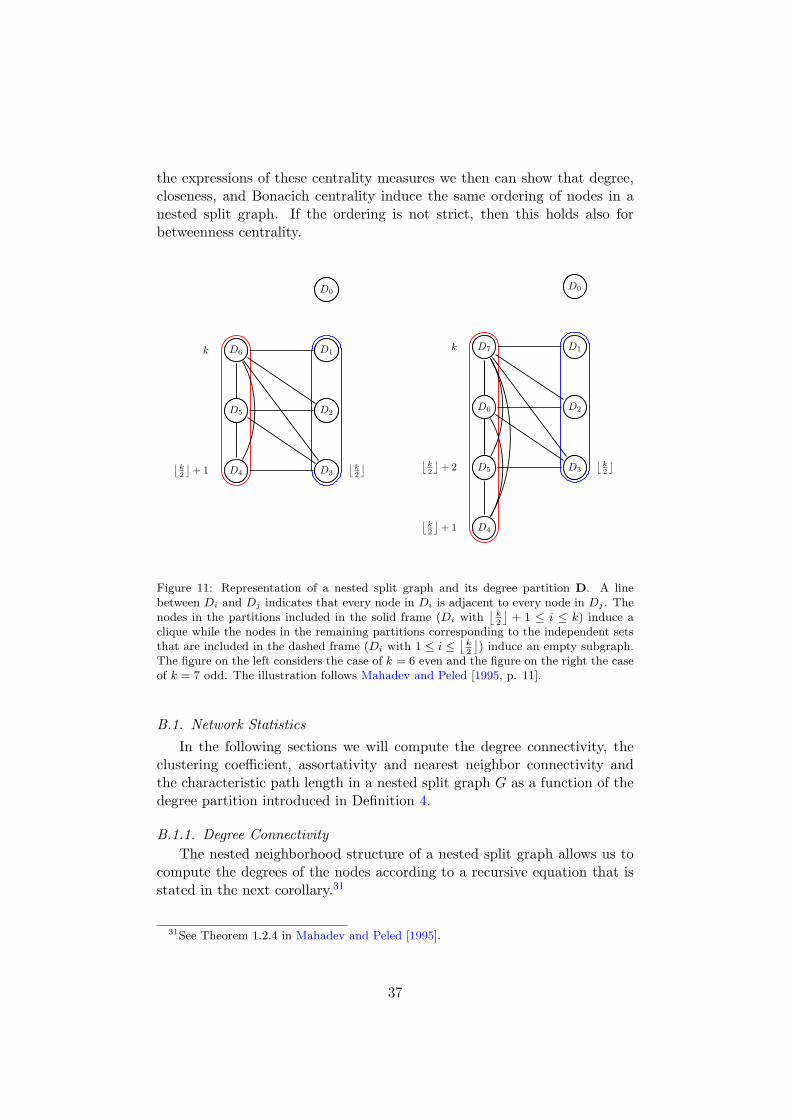
the expressions of these centrality measures we then can show that degree,closeness, and Bonacich centrality induce the same ordering of nodes in anested split graph. If the ordering is not strict, then this holds also forbetweenness centrality.
D0
D1
D2
D3D4
D5
D6
D0
D1
D2
D3
⌊
k2
⌋
D4
⌊
k2
⌋
+ 1
D5
D6k
D0
D1
D2
D3
D4
D5
D6
D7
D0
D1
D2
D3
D4
D5
D6
D7
⌊
k2
⌋⌊
k2
⌋
+ 2
⌊
k2
⌋
+ 1
k
Figure 11: Representation of a nested split graph and its degree partition D. A linebetween Di and Dj indicates that every node in Di is adjacent to every node in Dj . Thenodes in the partitions included in the solid frame (Di with
⌊
k2
⌋
+ 1 ≤ i ≤ k) induce aclique while the nodes in the remaining partitions corresponding to the independent setsthat are included in the dashed frame (Di with 1 ≤ i ≤
⌊
k2
⌋
) induce an empty subgraph.The figure on the left considers the case of k = 6 even and the figure on the right the caseof k = 7 odd. The illustration follows Mahadev and Peled [1995, p. 11].
B.1. Network Statistics
In the following sections we will compute the degree connectivity, theclustering coefficient, assortativity and nearest neighbor connectivity andthe characteristic path length in a nested split graph G as a function of thedegree partition introduced in Definition 4.
B.1.1. Degree Connectivity
The nested neighborhood structure of a nested split graph allows us tocompute the degrees of the nodes according to a recursive equation that isstated in the next corollary.31
31See Theorem 1.2.4 in Mahadev and Peled [1995].
37
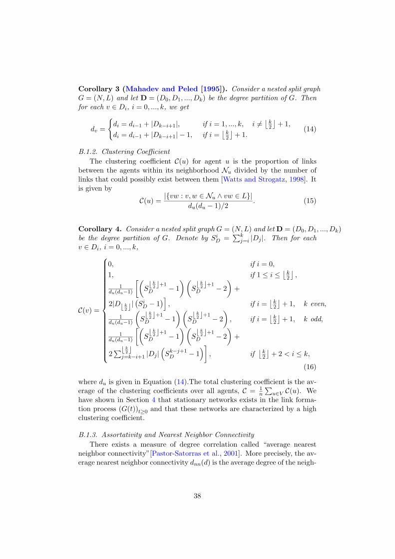
Corollary 3 (Mahadev and Peled [1995]). Consider a nested split graphG = (N, L) and let D = (D0, D1, ..., Dk) be the degree partition of G. Thenfor each v ∈ Di, i = 0, ..., k, we get
dv =
di = di−1 + |Dk−i+1|, if i = 1, ..., k, i 6=⌊
k2
⌋
+ 1,
di = di−1 + |Dk−i+1| − 1, if i =⌊
k2
⌋
+ 1.(14)
B.1.2. Clustering Coefficient
The clustering coefficient C(u) for agent u is the proportion of linksbetween the agents within its neighborhood Nu divided by the number oflinks that could possibly exist between them [Watts and Strogatz, 1998]. Itis given by
C(u) =|vw : v, w ∈ Nu ∧ vw ∈ L|
du(du − 1)/2. (15)
Corollary 4. Consider a nested split graph G = (N, L) and let D = (D0, D1, ..., Dk)be the degree partition of G. Denote by Si
D =∑k
j=i |Dj |. Then for eachv ∈ Di, i = 0, ..., k,
C(v) =
0, if i = 0,
1, if 1 ≤ i ≤⌊
k2
⌋
,
1du(du−1)
[(
S⌊ k
2⌋+1
D − 1
)(
S⌊ k
2⌋+1
D − 2
)
+
2|D⌊ k2⌋|(
SiD − 1
)
]
, if i =⌊
k2
⌋
+ 1, k even,
1du(du−1)
(
S⌊ k
2⌋+1
D − 1
)(
S⌊ k
2⌋+1
D − 2
)
, if i =⌊
k2
⌋
+ 1, k odd,
1du(du−1)
[(
S⌊ k
2⌋+1
D − 1
)(
S⌊ k
2⌋+1
D − 2
)
+
2∑⌊ k
2⌋j=k−i+1 |Dj |
(
Sk−j+1D − 1
)
]
, if⌊
k2
⌋
+ 2 < i ≤ k,
(16)
where du is given in Equation (14).The total clustering coefficient is the av-erage of the clustering coefficients over all agents, C = 1
n
∑
u∈V C(u). Wehave shown in Section 4 that stationary networks exists in the link forma-tion process (G(t))t≥0 and that these networks are characterized by a highclustering coefficient.
B.1.3. Assortativity and Nearest Neighbor Connectivity
There exists a measure of degree correlation called “average nearestneighbor connectivity”[Pastor-Satorras et al., 2001]. More precisely, the av-erage nearest neighbor connectivity dnn(d) is the average degree of the neigh-
38

bors of an agent with degree d. It is defined by
dnn(d) =∑
d′
d′P (d′|d), (17)
where P (d′|d) denotes the probability that an agent with degree d has aneighbor with degree d′.
Corollary 5. Consider a nested split graph G = (N, L) and let D = (D0, D1, ..., Dk)be the degree partition of G. Denote by Si
D =∑i
j=1 |Dk+1−j |. Then for eachv ∈ Di, i = 0, ..., k,
dnn(v) =
1Si
D
∑ij=1 |Dk+1−j |
(
Sk+1−jD − 1
)
, if i = 1, ...,⌊
k2
⌋
1
S⌊ k
2⌋+1
D−1
[
∑kj=⌊ k
2⌋+1|Dj |
(
SjD − 1
)
+|D⌊ k2⌋|S
⌊ k2⌋
D
]
, if i =⌊
k2
⌋
+ 1, k even,
1
S⌊ k
2⌋+1
D−1
[
∑kj=⌊ k
2⌋+1|Dj |
(
SjD − 1
)]
, if i =⌊
k2
⌋
+ 1, k odd,
1Si
D−1
[
∑kj=⌊ k
2⌋+1|Dj |
(
SjD − 1
)
+∑⌊ k
2⌋j=k−i+1 |Dj |Sj
D
]
, if i =⌊
k2
⌋
+ 2, ..., k
(18)
When the nearest neighbor connectivity is a monotonic increasing functionof the degree d, then the network is assortative, while, if it is monotonicdecreasing with d, it is dissortative [Newman, 2002; Pastor-Satorras et al.,2001]. Nested split graphs are dissortative, since for i < j and du ∈ Di <dv ∈ Dj it follows that dnn(u) > dnn(v). The higher is the degree of anagent in the cliques, the more neighbors it has from the independent setswith low degrees which decreases the average nearest neighbor connectivity.
B.1.4. Characteristic Path Length
The characteristic path length is defined as the number of links in theshortest path between two agents, averaged over all pairs of agents [Watts and Strogatz,1998]. This can be written as
L =1
n(n − 1)/2
∑
u 6=v
d(u, v), (19)
where d(u, v) is the geodesic (shortest path) between agent u and agent vin N . We do not consider the isolated agents in the set D0 because thecharacteristic path length is not defined for disconnected networks.
39
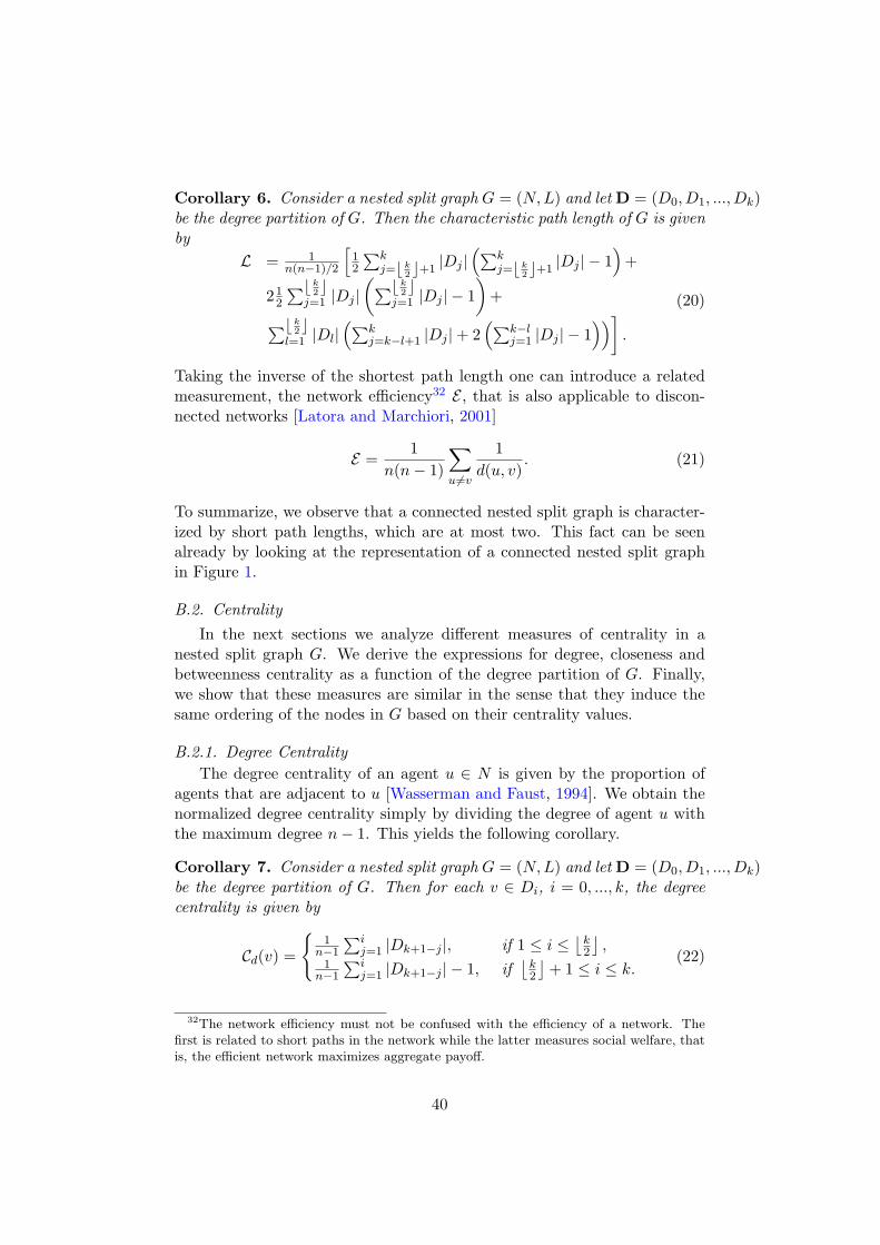
Corollary 6. Consider a nested split graph G = (N, L) and let D = (D0, D1, ..., Dk)be the degree partition of G. Then the characteristic path length of G is givenby
L = 1n(n−1)/2
[
12
∑kj=⌊ k
2⌋+1|Dj |
(
∑kj=⌊ k
2⌋+1|Dj | − 1
)
+
212
∑⌊ k2⌋
j=1 |Dj |(
∑⌊ k2⌋
j=1 |Dj | − 1
)
+
∑⌊ k2⌋
l=1 |Dl|(
∑kj=k−l+1 |Dj | + 2
(
∑k−lj=1 |Dj | − 1
))
]
.
(20)
Taking the inverse of the shortest path length one can introduce a relatedmeasurement, the network efficiency32 E , that is also applicable to discon-nected networks [Latora and Marchiori, 2001]
E =1
n(n − 1)
∑
u 6=v
1
d(u, v). (21)
To summarize, we observe that a connected nested split graph is character-ized by short path lengths, which are at most two. This fact can be seenalready by looking at the representation of a connected nested split graphin Figure 1.
B.2. Centrality
In the next sections we analyze different measures of centrality in anested split graph G. We derive the expressions for degree, closeness andbetweenness centrality as a function of the degree partition of G. Finally,we show that these measures are similar in the sense that they induce thesame ordering of the nodes in G based on their centrality values.
B.2.1. Degree Centrality
The degree centrality of an agent u ∈ N is given by the proportion ofagents that are adjacent to u [Wasserman and Faust, 1994]. We obtain thenormalized degree centrality simply by dividing the degree of agent u withthe maximum degree n − 1. This yields the following corollary.
Corollary 7. Consider a nested split graph G = (N, L) and let D = (D0, D1, ..., Dk)be the degree partition of G. Then for each v ∈ Di, i = 0, ..., k, the degreecentrality is given by
Cd(v) =
1n−1
∑ij=1 |Dk+1−j |, if 1 ≤ i ≤
⌊
k2
⌋
,1
n−1
∑ij=1 |Dk+1−j | − 1, if
⌊
k2
⌋
+ 1 ≤ i ≤ k.(22)
32The network efficiency must not be confused with the efficiency of a network. Thefirst is related to short paths in the network while the latter measures social welfare, thatis, the efficient network maximizes aggregate payoff.
40
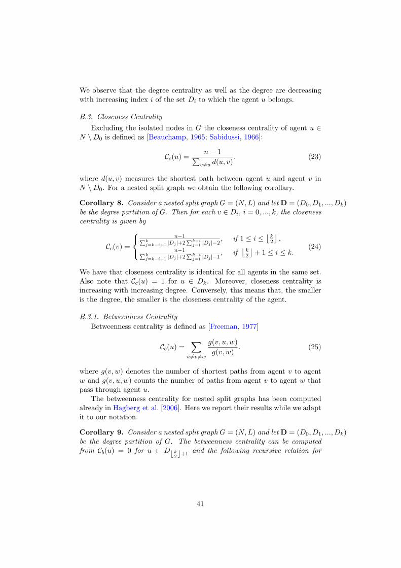
We observe that the degree centrality as well as the degree are decreasingwith increasing index i of the set Di to which the agent u belongs.
B.3. Closeness Centrality
Excluding the isolated nodes in G the closeness centrality of agent u ∈N \ D0 is defined as [Beauchamp, 1965; Sabidussi, 1966]:
Cc(u) =n − 1
∑
v 6=u d(u, v). (23)
where d(u, v) measures the shortest path between agent u and agent v inN \ D0. For a nested split graph we obtain the following corollary.
Corollary 8. Consider a nested split graph G = (N, L) and let D = (D0, D1, ..., Dk)be the degree partition of G. Then for each v ∈ Di, i = 0, ..., k, the closenesscentrality is given by
Cc(v) =
n−1∑k
j=k−i+1 |Dj |+2∑k−i
j=1 |Dj |−2, if 1 ≤ i ≤
⌊
k2
⌋
,
n−1∑k
j=k−i+1 |Dj |+2∑k−i
j=1 |Dj |−1, if
⌊
k2
⌋
+ 1 ≤ i ≤ k.(24)
We have that closeness centrality is identical for all agents in the same set.Also note that Cc(u) = 1 for u ∈ Dk. Moreover, closeness centrality isincreasing with increasing degree. Conversely, this means that, the smalleris the degree, the smaller is the closeness centrality of the agent.
B.3.1. Betweenness Centrality
Betweenness centrality is defined as [Freeman, 1977]
Cb(u) =∑
u 6=v 6=w
g(v, u, w)
g(v, w). (25)
where g(v, w) denotes the number of shortest paths from agent v to agentw and g(v, u, w) counts the number of paths from agent v to agent w thatpass through agent u.
The betweenness centrality for nested split graphs has been computedalready in Hagberg et al. [2006]. Here we report their results while we adaptit to our notation.
Corollary 9. Consider a nested split graph G = (N, L) and let D = (D0, D1, ..., Dk)be the degree partition of G. The betweenness centrality can be computedfrom Cb(u) = 0 for u ∈ D⌊ k
2⌋+1 and the following recursive relation for
41

u ∈ D⌊ k2⌋+1+(l+1) and v ∈ D⌊ k
2⌋+l+1
Cb(u) = Cb(v) +|D
k−(⌊ k2⌋+l+1)+1
|(
|Dk−(⌊ k
2⌋+l+1)+1|−1
)
∑k
j=(⌊ k2⌋+l+1)+1
|Dj |
+2|D
k−(⌊ k2⌋+l+1)+1
|[
∑(⌊ k
2⌋+l+1)−1
j=⌊ k2⌋+1
(|Dj |+|Dk−j+1|)+|D⌊ k2⌋+l+1
|]
∑k
j=(⌊ k2⌋+l+1)+1
|Dj |
(26)
with l = 0, ...,⌊
k2
⌋
− 1 if k is odd and l = 0, ...,⌊
k2
⌋
− 2 if k is even.
From Corollary 9 we find that the agents in the independent sets Di with1 ≤ i ≤
⌊
k2
⌋
have vanishing betweenness centrality. From the above equationwe also observe that the betweenness centrality is increasing with degreesuch that the agents in Dk have the highest betweenness centrality, theagents in Dk−1 the second highest betweenness centrality and so on. Thus,the ordering of betweenness centralities follows the degree ordering for allagents in the cliques while the agents in the independent sets have vanishingbetweenness centrality.
B.3.2. Eigenvector Centrality
There is a central property that holds for nested split graphs in relationto the Bonacich centrality, namely that the agents with higher degree alsohave higher Bonacich centrality. Similar to part (i) of Proposition 1 we cangive the following corollary.
Corollary 10. Let v be the eigenvector associated with the largest real eigen-value λPF of the adjacency matrix A of a nested split graph G = (N, L). Foreach i = 1, ..., n, vi is the eigenvector centrality of agent i. Consider a pairof agents i, j ∈ N . If and only if agent i has a higher degree than agent jthen i has a higher eigenvector centrality than j, i.e.
di > dj ⇔ vi > vj .
B.3.3. Centrality Rankings
We can make the following observation of the rankings of agents fordifferent centrality measures.
Corollary 11. Consider a nested split graph G = (N, L). Let Cd, Cc, Cb,Cv denote the degree, closeness, betweenness and eigenvector centrality in G.Then for any l, m ∈ d, c, v, l 6= m and i, j ∈ N we have that
Cl(i) ≥ Cl(j) ⇔ Cm(i) ≥ Cm(j), (27)
andCl(i) ≥ Cl(j) ⇒ Cb(i) ≥ Cb(j). (28)
42
If and only if an agent i has the k-th highest degree centrality then i isthe agent with the k-th highest closeness and eigenvector centrality. Thisresult also holds for Bonacich centrality (see Proposition 1). Moreover, if anagent i has the k-th highest degree centrality (this also holds for closeness,eigenvector and Bonacich centrality respectively) then it also has the k-thhighest betweenness centrality. The ordering induced by degree, closenesseigenvector and Bonacich centrality coincide and these orderings also applyin a weak sense for the betweenness centrality.
C. Capacity Constraints and Global Search
A natural generalization of the model discussed so far is to allow for thepossibility that agents are not accepting to establish a link from anotheragent that wants to connect to them. The underlying assumption is thatagents face capacity constraints in the number of links they can maintain.Such constraints can arise from a possible information overload and conges-tion [Arenas et al., 2008; Dodds et al., 2003; Fagiolo, 2005; Guimera et al.,2002; Huberman and Hogg, 1995]. In addition, we assume that agents arenot only searching for new contacts among their neighbors’ neighbors butalso among all agents in the network. However, agents preferably connectto their neighbors’ neighbors and only if this fails they search for new con-tacts at random. This means that, if capacity constraints prevent an agentfrom forming a link locally, we assume that she tries to link to an agent outof the whole population of agents at random. This mechanism introducesa global search mechanism in the link formation process (see Marsili et al.[2004]; Vega-Redondo [2006] for a similar approach). We find that by in-troducing capacity constraints and global search, differently to the basicmodel discussed in the previous sections, stationary networks can becomeassortative. Thus, we are able to reproduce all topological properties ofempirically observed social and economic networks. Moreover, the emer-gence of assortativity and positive degree-correlations respectively can beexplained by considering limitations in the number of links an agent canmaintain. This may be of particular relevance for social networks and givean explanation for the distinction between assortative social networks anddissortative technological networks suggested in Newman [2002].
We assume that capacity constraints arise from the fact that an agent canonly interact with one other agent out of her neighborhood at a time. Eachneighbor of an agent requests information with probability β.33 Assumingthat information requests are independent, the probability that an agent j ∈N with dj links does not receive any information requests from her neighborsis given by (1−β)dj . If an agent does not receive such an information request,
33If an agent has to process such a request, she cannot accept an additional link.
43
she can accept an additional link, otherwise not.Moreover, we allow for the formation of links between agents that are
not connected through a common neighbor. This means that agents searchglobally for new contacts if they cannot connect to the agent with highestcentrality among their neighbors’ neighbors. When an agent i is selected, shetries to connect to the agent j with the highest degree in her neighborhood.However, agent j ∈ Ni only accepts the link formation with probability(1 − β)dj , otherwise agent i selects another agent k ∈ N\ (Ni ∪ i, j) outof the whole population of agents (excluding agents i and j) uniformly atrandom, and this link also has the same acceptance probability (1 − β)dk
based on the degree of agent k.In the following we make two rather technical assumptions. First, for
the basic model in the previous sections the Bonacich centrality of an agentincreases the most if she forms a link to the agent with the highest degree.For the current model we will assume that this property is still approxi-mately true. In most cases this approximation can be made albeit thereexist exceptions in which the degree and Bonacich centrality ranking do notcoincide [Grassi et al., 2007].
Second, we further assume that if an agent is not free to accept anadditional link, (or the agent that is the target of the link can not forman additional link) another agent is selected, until a link is formed. In thisway, the values of α in the generalized model are comparable with the basicmodel without capacity constraints in which α is a measure of the networkdensity.
Taking into account the above mentioned capacity constraints in thenumber of links an agent can form and the possibility to form links outsidethe second order neighborhood, we generalize the link formation process(G(t))t≥0 introduced in Section 2.2 as follows:
Definition 7. We define the network formation process (G′(t))∞t=0 as a se-quence of networks, G′(0), G′(1), G′(2), ... in which at every step t = 0, 1, 2, ...,an agent i ∈ N = 1, 2, ..., n is uniformly selected at random, i ∼ U1, ..., n.Then one of the following events occurs:
(i) With probability pi = α agent i receives the opportunity to create an
additional link. Let j be the agent in N (2)i with the highest degree, that
is dj ≥ dk for all j, k ∈ N (2)i . Then with probability (1 − β)dj the link
ij is formed. Otherwise agent i connects to a randomly selected agentk ∈ N\ (Ni ∪ i, j) with probability
(
1 − (1 − β)dj)
(1−β)dk . If agenti is already connected to all other agents then nothing happens.
(ii) With probability qi = 1−pi = 1−α , the link to the agent j in Ni withthe smallest degree dj ≤ dk for all j, k ∈ Ni , decays. If agent i doesnot have any links then nothing happens.
44
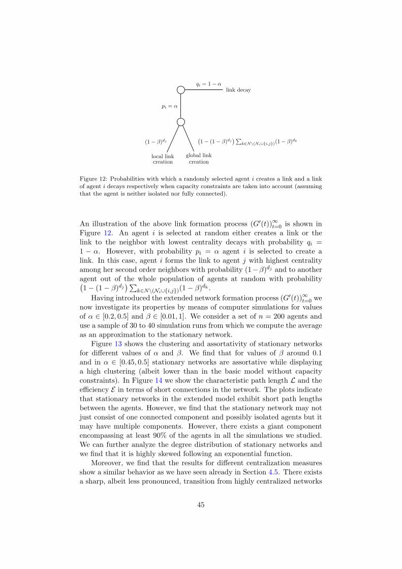
link decayqi = 1 − α
pi = α
local linkcreation
(1 − β)dj
global linkcreation
(
1 − (1 − β)dj)∑
k∈N\(Ni∪i,j)(1 − β)dk
Figure 12: Probabilities with which a randomly selected agent i creates a link and a linkof agent i decays respectively when capacity constraints are taken into account (assumingthat the agent is neither isolated nor fully connected).
An illustration of the above link formation process (G′(t))∞t=0 is shown inFigure 12. An agent i is selected at random either creates a link or thelink to the neighbor with lowest centrality decays with probability qi =1 − α. However, with probability pi = α agent i is selected to create alink. In this case, agent i forms the link to agent j with highest centralityamong her second order neighbors with probability (1−β)dj and to anotheragent out of the whole population of agents at random with probability(
1 − (1 − β)dj)∑
k∈N\(Ni∪i,j)(1 − β)dk .
Having introduced the extended network formation process (G′(t))∞t=0 wenow investigate its properties by means of computer simulations for valuesof α ∈ [0.2, 0.5] and β ∈ [0.01, 1]. We consider a set of n = 200 agents anduse a sample of 30 to 40 simulation runs from which we compute the averageas an approximation to the stationary network.
Figure 13 shows the clustering and assortativity of stationary networksfor different values of α and β. We find that for values of β around 0.1and in α ∈ [0.45, 0.5] stationary networks are assortative while displayinga high clustering (albeit lower than in the basic model without capacityconstraints). In Figure 14 we show the characteristic path length L and theefficiency E in terms of short connections in the network. The plots indicatethat stationary networks in the extended model exhibit short path lengthsbetween the agents. However, we find that the stationary network may notjust consist of one connected component and possibly isolated agents but itmay have multiple components. However, there exists a giant componentencompassing at least 90% of the agents in all the simulations we studied.We can further analyze the degree distribution of stationary networks andwe find that it is highly skewed following an exponential function.
Moreover, we find that the results for different centralization measuresshow a similar behavior as we have seen already in Section 4.5. There existsa sharp, albeit less pronounced, transition from highly centralized networks
45

0.01 0.1 1
β0
0.2
0.4
0.6
0.8
1
C
α=0.20α=0.40α=0.46α=0.47α=0.48α=0.50
0.01 0.1 1
β
-0.6
-0.4
-0.2
0
0.2
γ
α=0.20α=0.40α=0.46α=0.47α=0.48α=0.50
Figure 13: In the left panel we show the clustering coefficient obtained by recourse ofnumerical results of the extended model with capacity constrains for different values of αand β in a system with n = 200 agents. In the right panel we show the correspondingnetwork assortativity. Each different curve corresponds to a different value of α. Onlyagents that are not isolated are considered.
0.01 0.1 1
β0
1
2
3
4
5
6
L
α=0.20α=0.40α=0.46α=0.47α=0.48α=0.50
0.01 0.1 1
β0
0.2
0.4
0.6
0.8
1
ε
α=0.20α=0.40α=0.46α=0.47α=0.48α=0.50
Figure 14: We show the measures for the network topology obtained by recourse of nu-merical results of the model with capacity constrains for different values of α and β in asystem comprised of n = 200 agents. The left panel shows the characteristic path lengthL of the network G∗ and the right panel shows the results for the network efficiency E .
46
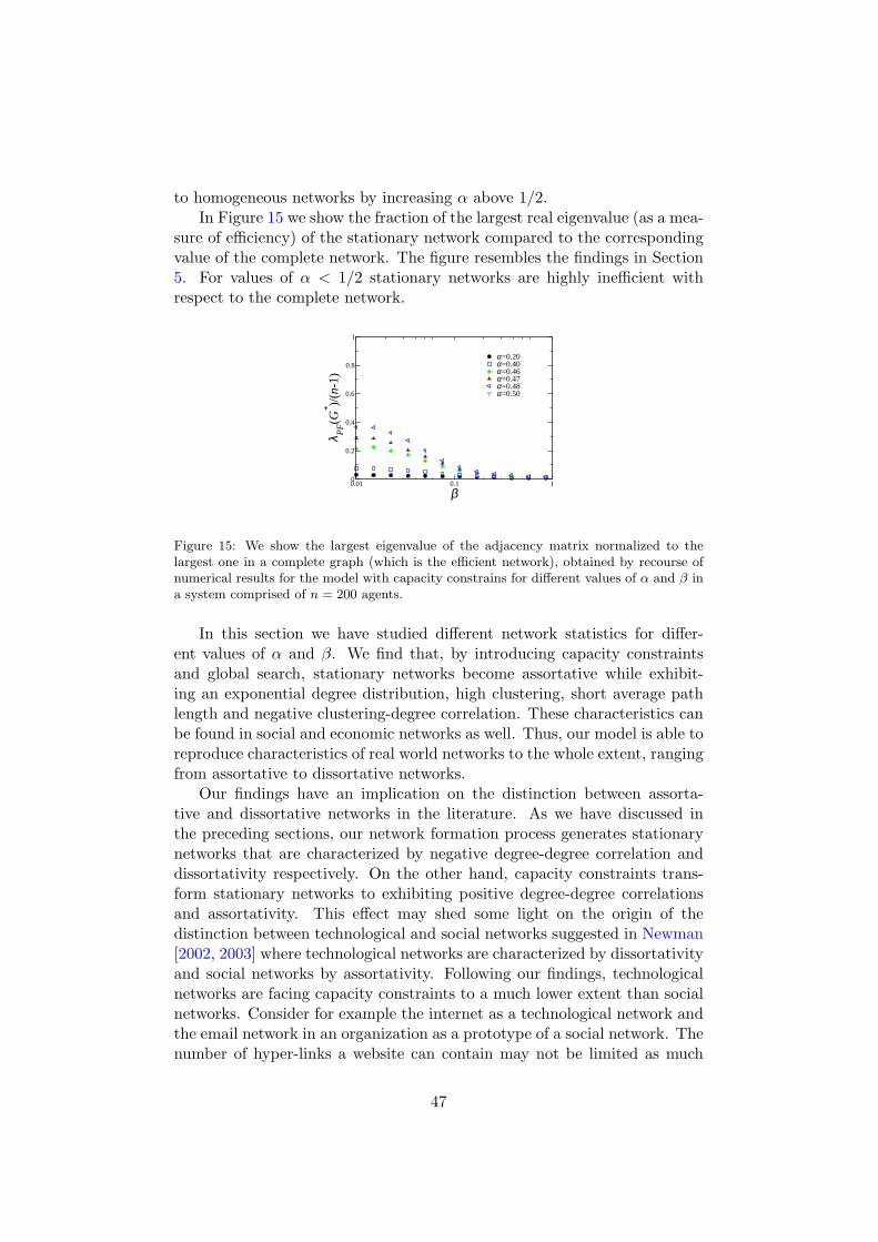
to homogeneous networks by increasing α above 1/2.In Figure 15 we show the fraction of the largest real eigenvalue (as a mea-
sure of efficiency) of the stationary network compared to the correspondingvalue of the complete network. The figure resembles the findings in Section5. For values of α < 1/2 stationary networks are highly inefficient withrespect to the complete network.
0.01 0.1 1
β0
0.2
0.4
0.6
0.8
1λ P
F(G
* )/(n
-1)
α=0.20α=0.40α=0.46α=0.47α=0.48α=0.50
Figure 15: We show the largest eigenvalue of the adjacency matrix normalized to thelargest one in a complete graph (which is the efficient network), obtained by recourse ofnumerical results for the model with capacity constrains for different values of α and β ina system comprised of n = 200 agents.
In this section we have studied different network statistics for differ-ent values of α and β. We find that, by introducing capacity constraintsand global search, stationary networks become assortative while exhibit-ing an exponential degree distribution, high clustering, short average pathlength and negative clustering-degree correlation. These characteristics canbe found in social and economic networks as well. Thus, our model is able toreproduce characteristics of real world networks to the whole extent, rangingfrom assortative to dissortative networks.
Our findings have an implication on the distinction between assorta-tive and dissortative networks in the literature. As we have discussed inthe preceding sections, our network formation process generates stationarynetworks that are characterized by negative degree-degree correlation anddissortativity respectively. On the other hand, capacity constraints trans-form stationary networks to exhibiting positive degree-degree correlationsand assortativity. This effect may shed some light on the origin of thedistinction between technological and social networks suggested in Newman[2002, 2003] where technological networks are characterized by dissortativityand social networks by assortativity. Following our findings, technologicalnetworks are facing capacity constraints to a much lower extent than socialnetworks. Consider for example the internet as a technological network andthe email network in an organization as a prototype of a social network. Thenumber of hyper-links a website can contain may not be limited as much
47

as the number of social contacts (measured e.g. by mutual email exchange)an individual in an organization may keep. Thus, the distinction betweentechnological and social networks and the degree of assortativity and degree-degree correlations can be derived from the severity of capacity constraintsimposed on the number of links an agent can maintain.
D. Proofs of Propositions, Corollaries and Lemmas
In this section we give the proofs of the propositions, corollaries and lemmasstated earlier in the paper.
Proof of Proposition 1.
(i) A graph having a stepwise adjacency matrix is a nested split graphG. A nested split graph has a nested neighborhood structure. Theneighborhood Nj of an agent j is contained in the neighborhood Ni
of the next higher degree agent i with |Ni| = di > |Nj | = dj withNj ⊂ Ni. For a symmetric adjacency matrix the vector of Bonacichcentralities is given by b(G, λ) = λAb + u, u = (1, ..., 1)T . For anagent i = 1, ..., n we get
bi(G, λ) = λn∑
k=1
aikbk(G, λ) + 1 = λ∑
k∈Ni
bk(G, λ) + 1, (29)
and similarly for agent j
bj(G, λ) = λ∑
k∈Nj
bk(G, λ) + 1. (30)
Since Nj ⊂ Ni and dj = |Nj | < |Ni| = di we get
bi(G, λ)
bj(G, λ)=
λ∑
k∈Nibk(G, λ) + 1
λ∑
k∈Njbk(G, λ) + 1
> 1. (31)
The inequality follows from the fact that the Bonacich centrality isnonnegative and the numerator contains the sum over the same posi-tive numbers as the denominator plus some additional values.
Conversely, in a nested split graph we must either have Ni ⊂ Nj orNj ⊂ Ni. Assuming that bi(G, λ) > bj(G, λ) we can conclude fromthe above equation that Nj ⊂ Ni and therefore |Ni| = di > |Nj | = dj .If there are l distinct degrees in G then the ordering of degrees d1 >d2 > ... > dl is equivalent to the ordering of the Bonacich centralitiesb1(G, λ) > b2(G, λ) > ... > bl(G, λ).
(ii) Consider the agents i, j and k in the nested split graph G(t), suchthat dj ≤ dk. Let G′ be the graph obtained from G(t) by adding the
48
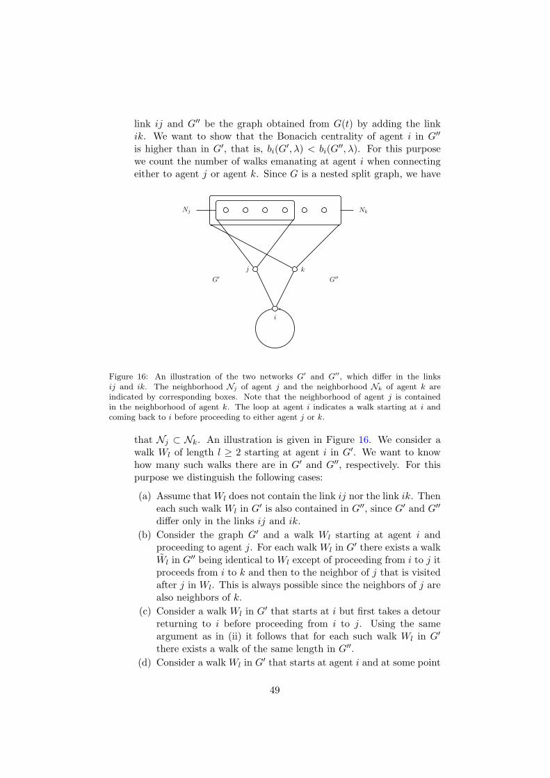
link ij and G′′ be the graph obtained from G(t) by adding the linkik. We want to show that the Bonacich centrality of agent i in G′′
is higher than in G′, that is, bi(G′, λ) < bi(G
′′, λ). For this purposewe count the number of walks emanating at agent i when connectingeither to agent j or agent k. Since G is a nested split graph, we have
i
j k
Nj Nk
G′ G′′
Figure 16: An illustration of the two networks G′ and G′′, which differ in the linksij and ik. The neighborhood Nj of agent j and the neighborhood Nk of agent k areindicated by corresponding boxes. Note that the neighborhood of agent j is containedin the neighborhood of agent k. The loop at agent i indicates a walk starting at i andcoming back to i before proceeding to either agent j or k.
that Nj ⊂ Nk. An illustration is given in Figure 16. We consider awalk Wl of length l ≥ 2 starting at agent i in G′. We want to knowhow many such walks there are in G′ and G′′, respectively. For thispurpose we distinguish the following cases:
(a) Assume that Wl does not contain the link ij nor the link ik. Theneach such walk Wl in G′ is also contained in G′′, since G′ and G′′
differ only in the links ij and ik.
(b) Consider the graph G′ and a walk Wl starting at agent i andproceeding to agent j. For each walk Wl in G′ there exists a walkWl in G′′ being identical to Wl except of proceeding from i to j itproceeds from i to k and then to the neighbor of j that is visitedafter j in Wl. This is always possible since the neighbors of j arealso neighbors of k.
(c) Consider a walk Wl in G′ that starts at i but first takes a detourreturning to i before proceeding from i to j. Using the sameargument as in (ii) it follows that for each such walk Wl in G′
there exists a walk of the same length in G′′.(d) Consider a walk Wl in G′ that starts at agent i and at some point
49
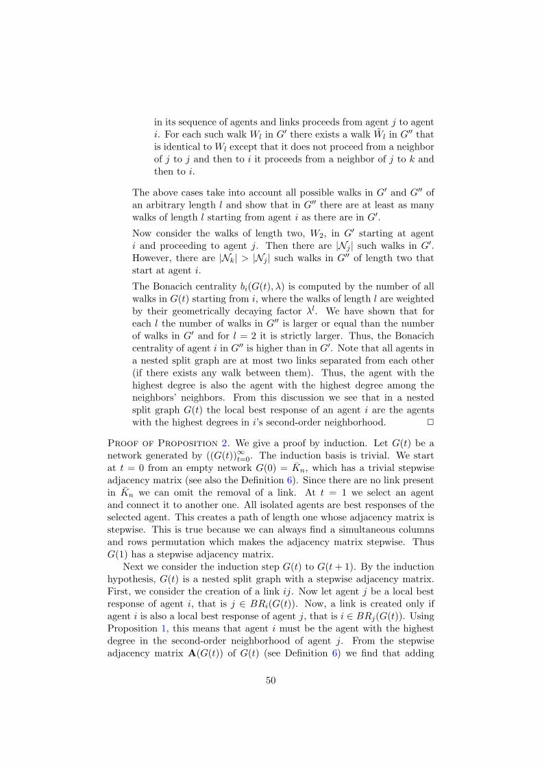
in its sequence of agents and links proceeds from agent j to agenti. For each such walk Wl in G′ there exists a walk Wl in G′′ thatis identical to Wl except that it does not proceed from a neighborof j to j and then to i it proceeds from a neighbor of j to k andthen to i.
The above cases take into account all possible walks in G′ and G′′ ofan arbitrary length l and show that in G′′ there are at least as manywalks of length l starting from agent i as there are in G′.
Now consider the walks of length two, W2, in G′ starting at agenti and proceeding to agent j. Then there are |Nj | such walks in G′.However, there are |Nk| > |Nj | such walks in G′′ of length two thatstart at agent i.
The Bonacich centrality bi(G(t), λ) is computed by the number of allwalks in G(t) starting from i, where the walks of length l are weightedby their geometrically decaying factor λl. We have shown that foreach l the number of walks in G′′ is larger or equal than the numberof walks in G′ and for l = 2 it is strictly larger. Thus, the Bonacichcentrality of agent i in G′′ is higher than in G′. Note that all agents ina nested split graph are at most two links separated from each other(if there exists any walk between them). Thus, the agent with thehighest degree is also the agent with the highest degree among theneighbors’ neighbors. From this discussion we see that in a nestedsplit graph G(t) the local best response of an agent i are the agentswith the highest degrees in i’s second-order neighborhood. 2
Proof of Proposition 2. We give a proof by induction. Let G(t) be anetwork generated by ((G(t))∞t=0. The induction basis is trivial. We startat t = 0 from an empty network G(0) = Kn, which has a trivial stepwiseadjacency matrix (see also the Definition 6). Since there are no link presentin Kn we can omit the removal of a link. At t = 1 we select an agentand connect it to another one. All isolated agents are best responses of theselected agent. This creates a path of length one whose adjacency matrix isstepwise. This is true because we can always find a simultaneous columnsand rows permutation which makes the adjacency matrix stepwise. ThusG(1) has a stepwise adjacency matrix.
Next we consider the induction step G(t) to G(t + 1). By the inductionhypothesis, G(t) is a nested split graph with a stepwise adjacency matrix.First, we consider the creation of a link ij. Now let agent j be a local bestresponse of agent i, that is j ∈ BRi(G(t)). Now, a link is created only ifagent i is also a local best response of agent j, that is i ∈ BRj(G(t)). UsingProposition 1, this means that agent i must be the agent with the highestdegree in the second-order neighborhood of agent j. From the stepwiseadjacency matrix A(G(t)) of G(t) (see Definition 6) we find that adding
50
Figure 17: Two possible positions for the creation of a link from agent 4, either to agent 7or to agent 10, are indicated with boxes. Agent 7 has degree 3 while agent 10 has degree1. Creating a link to an agent with higher degree results in higher equilibrium payoffs.Thus, the best response of agent 4 is agent 7 and not agent 10.
the link ij to the network G(t) such that both agents are the agents withthe highest degrees in their second-order neighborhoods results in a matrixA(G(t) + ij) that is stepwise. Therefore, the network G(t) + ij is a nestedsplit graph.
We give an example in Figure 17. Let the agents be numbered by therows respectively columns of the adjacency matrix. We assume that agent4 is selected to create a link. Two possible positions for the creation of alink from agent 4, either to agent 7 or to agent 10 are indicated with boxes.Since, in a stepwise matrix, the best response agent has the highest degree,agent 7 is a best response of agent 4 while agent 10 is not. We now canturn to the best response of agent 7. The agents not connected to agent 7are indicated by zero entries in the seventh column of the adjacency matrix.There we find that agent 4 is also a best response of agent 7, since agent4 is the agent with the highest degree not already connected to agent 7.Finally, we observe that creating the link 47 preserves the stepwise form ofthe adjacency matrix (see also Definition 6).34
For the removal of a link a similar argument can be applied as in thepreceding discussion. Disconnecting from the agent with the smallest degreedecreases the Bonacich centrality and equilibrium payoffs the least. Fromthe properties of the stepwise matrix A(G(t)) it then follows that the matrixA(G(t) − ij) is stepwise.
Thus, in any step t in the network formation process (G(t))∞t=0, G(t) isa nested split graph with an associated stepwise adjacency matrix A(G(t)).
2
34The adjacency matrix is uniquely defined up to a permutation of its rows and columns.Applying such a permutation, we can always find an adjacency matrix which is stepwise.
51
Proof of Corollary 1. In Proposition 2 we have shown that G(t) gen-erated by (G(t))∞t=0 is a nested split graph for all t. Thus, from the charac-terization of a nested split graph given in Definition 5 we know that G(t) hasa nested neighborhood structure. This implies that for any node with degreed there exists a path to any other node with a (positive) degree smaller thand, and vice versa. This holds for any degree d in a nested split graph. Itfollows that G(t) consists of a connected component and possible isolatednodes. 2
Proof of Proposition 3. We will show that the network formation pro-cess (G(t))∞t=0 introduced in Definition 3 induces a Markov chain on a finitestate space Ω. Ω contains all unlabeled nested split graphs with n nodes.It can be shown that |Ω| = 2n−1 [Mahadev and Peled, 1995]. Therefore,the number of states is finite and the transition between states can be rep-resented with a transition matrix P. In the following we show that thisMarkov chain is irreducible and aperiodic. We then say that (G(t))∞t=0 is er-godic. Further this means that there exists a unique stationary distributionµ satisfying µP = µ [see e.g. Seneta, 1973, 2006].
First we show that (G(t))∞t=0 is a Markov chain. The network G(t+1) ∈ Ωis obtained from G(t) by removing or adding a link to G(t). Thus, theprobability of obtaining G(t + 1) depends only on G(t) and not on theprevious networks for t′ < t, that is
P (G(t + 1) = Gj |G(0) = Gi0 , G(1) = Gi1 , ..., G(t) = Git) =
P (G(t + 1) = Gj |G(t) = Git) . (32)
The number of possible networks G(t) is finite for any time t and the tran-sition probabilities from a network G(t) to G(t + 1) do not depend on t.Therefore, (G(t))∞t=0 is a finite state, discrete time, homogeneous Markovchain.
Next, we show that (G(t))∞t=0 is irreducible. Consider two networksG, G′ ∈ Ω. (G(t))∞t=0 is irreducible if there exists a positive probability topass from any G to any other G′ in Ω. We say that G′ is accessible from G.For any G there exists a positive probability that in all consecutive steps inthe Markov chain links are removed and no links are created until the emptynetwork Kn ∈ Ω is reached. Then there exists a positive probability thatfrom Kn only those links are created that generate exactly the network G′.Therefore, there exists a positive probability to pass from any network G toany other network G′ with positive probability. Similarly, one can show thatG is accessible from G′. States G and G′ are accessible from one-another.We say that they communicate and Ω is a communicating class.
Moreover, the Markov process is aperiodic. Observe that with positiveprobability the empty network Kn can stay empty in the next time step.This happens when an agent is selected for removing a link, which happens
52
with probability 1 − α. Since she has no links, nothing happens. Thus, thestate Kn is aperiodic. The existence of an aperiodic state in the commu-nicating class Ω implies that the Markov process induced by (G(t))∞t=0 isaperiodic.
Since we have shown that (G(t))∞t=0 induces a finite Markov chain that isirreducible and aperiodic, this Markov chain is ergodic. Moreover, it followsthat there exists a unique stationary distribution µ. 2
Proof of Proposition 4. We consider the network formation process (G(t))∞t=0
on Ω introduced in Definition 3. At every step t = 0, 1, 2, ... a link is createdwith probability α and a link is removed with probability 1 − α. Further,we consider the complementary network formation process (G′(t))∞t=0 on Ωwhere in every period t a link is created with probability α′ = 1 − α anda link is removed with probability 1 − α′ = α. This means that a link isremoved in (G′(t))∞t=0 whenever a link is created in (G(t))∞t=0 and a link iscreated whenever a link is removed in (G(t))∞t=0.
35
As an example, consider the network G represented by the adjacencymatrix A in Figure 17. The complement G has an adjacency matrix Aobtained from A by replacing each one element in A by zero and each zeroelement by one, except for the elements on the diagonal. Let H be thenetwork obtained from G by adding the link 47 (setting a47 = a74 = 1 inA). The probability of this link being created and thus the probability ofreaching H after the process was in G is 3α
n , either by selecting one of thetwo nodes with degrees three or the node with degree five to create a link.Observe that this is identical to the probability of reaching the network Hfrom G if either the two nodes with degrees seven or the node with degreefour in G are selected to remove a link (with probability α′ = 1 − α).
In general we can say that, for any G1, G2 ∈ Ω we have that
P (G(t + 1) = G2|G(t) = G1) = P(
G′(t + 1) = G2|G′(t) = G1
)
. (33)
Next consider the stationary distribution µ of (G(t))∞t=0 and the correspond-ing transition matrix P. Similarly, consider the stationary distribution µ′ of(G′(t))∞t=0 and the corresponding transition matrix P′. Consider an order-ing of states G1, G2, ... in Ω and the transition matrix P with elements pij
giving the probability of observing Gj after the Markov process (G(t))∞t=0
35Two nodes of G′(t) are adjacent if and only if they are not adjacent in G(t). Note thatthe complement of a nested split graph is a nested split graph as well [Mahadev and Peled,1995]. In particular, the networks G′(t) are nested split graphs in which the number ofnodes in the dominating sets corresponds to the number of nodes in the independent setsin G(t) and the number of nodes in the independent sets in G′(t) corresponds to thenumber of nodes in the dominating sets in G(t). Thus, (G′(t))
∞
t=0 has the same statespace Ω as (G(t))∞
t=0, namely the space consisting all unlabeled nested split graphs on nnodes.
53
was in Gi. Similarly, consider an ordering of states G1, G2, ... in Ω and thetransition matrix P′ with elements p′ij giving the probability of observing
Gj after the Markov process (G′(t))∞t=0 was in Gi. Equation (33) impliesthat P = P′. Moreover, for the stationary distributions it must hold thatµP = µ and µ′P′ = µ′. Since P is irreducible and aperiodic, P has a uniquepositive eigenvector and therefore µ′ = µ. It follows that for any networkG with probability µG generated by (G(t))∞t=0 we can take the complementG = G′ and assign it the probability µG to get the corresponding probabilityin µ′, i.e. µG = µ′
G′ . 2
Proof of Proposition 5. Before we proceed with the proof of Proposi-tion 5, we give three useful lemmas.
Lemma 1. Let N(t)∞t=0 be the degree distribution with the d-th elementNd(t) in the t-th sequence N(t) = Nd(t)n−1
d=0 . Then for any ǫ > 0 we havethat
P
(∣
∣
∣
∣
Nd(t)
n− E
(
Nd(t)
n
)∣
∣
∣
∣
≥ ǫ
)
≤ 2e−ǫ2n2
8t . (34)
Further, denoting by nd = limt→∞Nd(t)
n the asymptotic proportion of nodeswith degree d and setting t = n, Equation (34) implies that limn→∞ P (nd − E(nd)) =0.
Proof of Lemma 1. N(t)∞t=0 is a Markov chain. Moreover, the changein the number of nodes with degree d per period t is bounded by one, i.e.|Nd(t)−Nd(t− 1)| ≤ 2, since at most one link is added or removed in everyperiod t. Now we define the following random variable
Ys = E (Nd(t)|N(s)) . (35)
Since N(t)∞t=0 is a Markov chain, the sequence Ysts=0 is a Doob’s mar-
tingale with respect to N(t)∞t=0 [see e.g. Grimmett and Stirzaker, 2001].Therefore, we can apply Hoeffding’s inequality [Grimmett and Stirzaker,2001], which states that for any 0 < s ≤ t with |Ys−Ys−1| ≤ c and any ǫ > 0
P (|Yt − Y0| > ǫ) ≤ 2e−ǫ2
2tc2 . (36)
With Yt = E (Nd(t)|N(t)) = Nd(t) and Y0 = E (Nd(t)|N(0)) = E (Nd(t)) itfollows from Equation (36) that
P
(∣
∣
∣
∣
Nd(t)
n− E
(
Nd(t)
n
)∣
∣
∣
∣
≥ ǫ
)
= P (|Nd(t) − E (Nd(t))| ≥ nǫ) ≤ 2e−ǫ2n2
8t .
(37)
This implies that the empirical proportion Nd(t)n of nodes with degree d
converges in probability to its expected value E(
Nd(t)n
)
as n becomes large.
54
Lemma 2. Consider the ergodic Markov chain (G(t))∞t=0 and state space Ωconsisting of all nested split graphs. Let X denote the set of states in Ω inwhich there is exactly one node with degree d + 1 and Y the set of stateswhere there is no node with degree d + 1. Denote by µ(X) the probabilityof the states in X in the stationary distribution µ of (G(t))∞t=0 and by µ(Y )the probability of states in Y . If the number of nodes with degree Nd in Yis O(n) such that limn→∞
Nd
n > 0 then limn→∞ µ(Y ) = 0.36
Proof of Lemma 2. Let N(X, Y, y) be the expected number of times statesin X occur before the process reaches Y (not counting the process as havingimmediately reached Y if y ∈ Y ) when the process starts in y. Then thefollowing relation holds (see Theorem 6.2.3 in Kemeny and Snell [1960] andalso Ellison [2000])
µ(X)
µ(Y )= N(X, Y, y). (38)
Let pY X denote a lower bound on the probability that a state in X occursafter the process is in a state in Y and, conversely, let pXY denote theprobability that a state in Y occurs after the process is in a state in X.This probability is the same for all states in X, since from the properties ofthe Markov chain (G(t))∞t=0, it follows that pXY = 2(1−α)
n (there exist twoways to remove the link of the node with degree d + 1 and the probabilityto select a node for link removal is 1−α
n ). Then we can write
N(X, Y, y) ≥ pY XpXY
+ 2pY X(1 − pXY )pXY
+ 3pY X(1 − pXY )2pXY
+ ...
= pY XpXY
∞∑
i=1
i(1 − pXY )i−1
=pY X
pXY.
The right hand side of the above inequality takes into account the fact thatstates in X can be reached once, twice, etc., before a state in Y is reachedand assigns the corresponding probabilities to compute the expected value.
By assuming that there exists a number Nd of nodes with degree d which
36By f = O(g) we mean that lim supn→∞
∣
∣
∣
f(n)g(n)
∣
∣
∣< ∞.
55
is O(n), say Nd = βn, we have that pY X = αβ > 0.37 It then follows that
µ(X)
µ(Y )= N(X, Y, y) ≥ pY X
pXY=
αβ
2(1 − α)n −−−→
n→∞∞, (39)
and therefore limn→∞ µ(Y ) = 0. 2
Lemma 3. For 0 ≤ α ≤ 1/2 the asymptotic average number of isolatednodes is n0 = n+α−2nα
(1−α)n .
Proof of Lemma 3. We consider the expected change in the number oflinks M(t) = 1
2
∑n−1d=0 Nd(t)d from t to t + 1. The number of links increases
by one if an isolated node is selected for creating a link. This happens withprobability α
n (n − Nn−1(t)), where Nn−1 denotes the number of maximallyconnected nodes with degree n−1. The number of links decreases whenevera node with degree higher than zero (in the connected component) is selectedfor removing a link. This happens with probability 1−α
n (n − N0(t)), whereN0 denotes the number of isolated nodes. Putting the above contributionstogether we can write for the expected change in the total number M(t) oflinks
E (M(t + 1)|N(t)) = M(t) +α
n(n − Nn−1(t)) −
1 − α
n(n − N0(t)) (40)
By means of Lemma 1, we know that in the limit of large n, the empiricaldegree distribution converges to the expected degree distribution in proba-bility. This also applies for the number of links, since M(t) is a continuousfunction of N(t) and N(t) converges in probability to its expected value.Denote by m(t) = E (M(t)). Then the above equation gives a relationshipbetween the asymptotic average number of nodes of degree zero and one,respectively,
(1 − 2α) = (1 − α)n0 − αnn−1. (41)
Next, we consider the process (G′(t))∞t=0 which is constructed from (G(t))∞t=0
by taking the complement of each network G(t) in every period t (see also theproof of Proposition 4). Denote the expected number of links in (G(t))∞t=0
by m and in (G′(t))∞t=0 by m′. By construction, we must have that m =n(n−1)
2 −m′. From Proposition 4 we know that the Markov process (G′(t))∞t=0
has the same stationary distribution µ′ as a process from Definition 3 for alink creation probability of α′ = 1 − α. For α = 1/2 the two processes are
37By assumption the expected value of Nd proportional to n. Thus, a state with finiteNd must be reached with positive probability. Further, in such a state, there exists apositive probability that a transition occurs from Y to X, because we can always selecta node with degree d to create a node with degree d + 1. This happens with probabilitypY X = α
nNd = αβ.
56
identical and we must have that also their expected number of links are thesame. This implies that for α = 1/2, m = m′ = n(n−1)
4 . The only nestedsplit graph with this number of links, for which the complement has the samenumber of links as the original graph, is the one in which each independentset is of size one and also each dominating set has size one (except possiblyfor the set corresponding to the
(⌊
k2
⌋
+ 1)
-th partition). Thus, for α = 1/2it must hold that n0 = nn−1 = 1
n .Moreover, we know that for α < 1/2 the expected number of maximally
connected nodes (with degree n − 1) is at most as large as the expectednumber for α = 1/2, since the probability of links being created strictlydecreases while the probability of links being removed increases for valuesof α below 1/2 (and the probability of a maximally connected node losing alink strictly increases). Thus, for large n we can write
(1 − 2α)n = (1 − α)n0 −α
n. (42)
For α below 1/2 the last term on the right hand side of Equation (42) canbe neglected for large n while it is exact for α = 1/2 (where Equation (42)gives n0 = 1).38 Therefore, Equation (42) holds for any value of α if n islarge enough. From Equation (42) we then obtain
n0 =n + α − 2nα
(1 − α)n, (43)
with the limits limα→0 n0 = 1 and limα→1/2 n0 = 1n . 2
With these three lemmas at hand, we are now able to prove Proposition5. Let N(t)∞t=0 be the degree distribution with the d-th element Nd(t)in the t-th sequence N(t) = Nd(t)n−1
d=0 . Note that from the properties of(G(t))∞t=0 (G(t) is completely determined by N(t) and vice versa) it follows
that N(t)∞t=0 is a Markov chain. Denote by nd(t) = E(
Nd(t)n
)
the expected
proportion of nodes with degree d. Further, denote by nd = limt→∞ nd(t)the asymptotic expected proportion of nodes with degree d. nd is determinedby the invariant distribution µ in the limit of large times t. We show byinduction that, given nd−1 and nd are Θ(1) as n becomes large, also nd+1 isΘ(1) for all 0 ≤ d < d∗, in the limit of large n.39 For this purpose we consider(a) the expected number of isolated nodes E (N0(t + 1)|N(t)) and (b) the
38If α < 1/2 then we can write (1 − 2α) = (1 − α)n0 − α/n ∼ (1 − α)n0 for n large.This also holds for any nn−1 ≤ 1/n. On the other hand, for α = 1/2, also n0 = 1/n andthe term α/n in Equation (42) can no longer be neglected.
39By f = Θ(g) we mean that lim infn→∞
∣
∣
∣
f(n)g(n)
∣
∣
∣≤ lim supn→∞
∣
∣
∣
f(n)g(n)
∣
∣
∣< ∞. In particu-
lar, f = Θ(1) implies that limn→∞f(n) > 0.
57
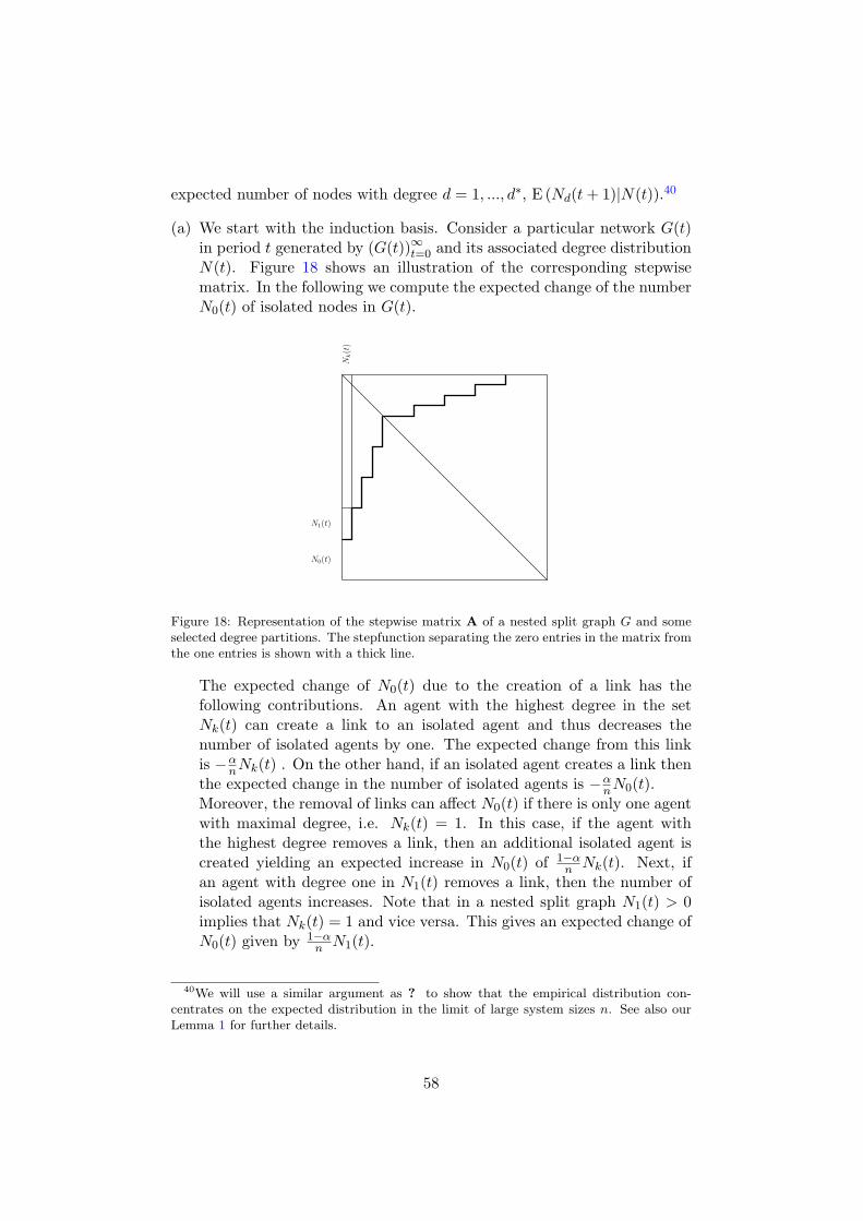
expected number of nodes with degree d = 1, ..., d∗, E (Nd(t + 1)|N(t)).40
(a) We start with the induction basis. Consider a particular network G(t)in period t generated by (G(t))∞t=0 and its associated degree distributionN(t). Figure 18 shows an illustration of the corresponding stepwisematrix. In the following we compute the expected change of the numberN0(t) of isolated nodes in G(t).
N0(t)
N1(t)
Nk(t
)
Figure 18: Representation of the stepwise matrix A of a nested split graph G and someselected degree partitions. The stepfunction separating the zero entries in the matrix fromthe one entries is shown with a thick line.
The expected change of N0(t) due to the creation of a link has thefollowing contributions. An agent with the highest degree in the setNk(t) can create a link to an isolated agent and thus decreases thenumber of isolated agents by one. The expected change from this linkis −α
nNk(t) . On the other hand, if an isolated agent creates a link thenthe expected change in the number of isolated agents is −α
nN0(t).Moreover, the removal of links can affect N0(t) if there is only one agentwith maximal degree, i.e. Nk(t) = 1. In this case, if the agent withthe highest degree removes a link, then an additional isolated agent iscreated yielding an expected increase in N0(t) of 1−α
n Nk(t). Next, ifan agent with degree one in N1(t) removes a link, then the number ofisolated agents increases. Note that in a nested split graph N1(t) > 0implies that Nk(t) = 1 and vice versa. This gives an expected change ofN0(t) given by 1−α
n N1(t).
40We will use a similar argument as ? to show that the empirical distribution con-centrates on the expected distribution in the limit of large system sizes n. See also ourLemma 1 for further details.
58
Putting the above contributions together, the expected number of iso-lated nodes at time t + 1, given N(t), is given by the following expres-sion41
E (N0(t + 1)|N(t)) =
N0(t) −α
n(N0(t) + Nk(t)) +
1 − α
n(N1(t) + 1) δNk(t),1. (44)
By means of Lemma 1, we know that in the limit of large n, the empir-ical degree distribution converges to the expected degree distribution inprobability. Moreover, for large t the expectation is computed on thebasis of the invariant distribution µ. Note that from Lemma 3 we knowthat the asymptotic expected proportion n0 of isolated nodes is Θ(1),for n large. Thus we can apply the result of Lemma 2 which tells usthat the networks in which there does not exist a node with degree onehave vanishing probability in µ for large n. Since the existence of a nodewith degree one implies that Nk(t) = 1, in the limit of large n we canset limt→∞ δNk(t),1 = 1. Then we obtain from Equation (44)
n0 =1 − α
αn1 +
1 − 2α
αn. (45)
Note that since n0 is Θ(1) (see Lemma 3) we also have that n1 is Θ(1)as n grows.
(b) We give a proof by induction on the number Nd(t) of nodes with de-gree 0 < d < d∗ in a network G(t) in the support of the stationarydistribution µ. We give an illustration in Figure 19. In the following,we compute the expected change in Nd(t) due to the creation or theremoval of a link.Let us investigate the creation of a link. With probability α
n a link iscreated from the agent in Nk−d to an agent in Nd(t). This yields acontribution to the expected change of Nd(t) of −α
nNk−d. If a link iscreated from an agent in Nk−d+1 to an agent in Nd(t) then the expectedchange is α
n , if Nk−d+1 contains only a single agent . Similarly, if a link iscreated from an agent in Nd−1(t) to the agent in Nd(t) then the expectedchange of Nd(t) is α
nNd−1(t), if Nk−d+1 = 1. Moreover, if an agent inNd(t) is selected for link creation, then we get an expected decrease of−α
nNd(t).Now we consider the removal of a link. If a link is removed from theagent in Nk−d+1 to an agent in Nd then the expected change of Nd(t)is −1−α
n Nk−d+1. If a link is removed from an agent in Nk−d to an agentin Nd+1(t) then the expected increase of Nd(t) is 1−α
n , if Nk−d = 1.
41δi,j denotes the usual Kronecker delta which is 1 if i = j and 0 otherwise.
59
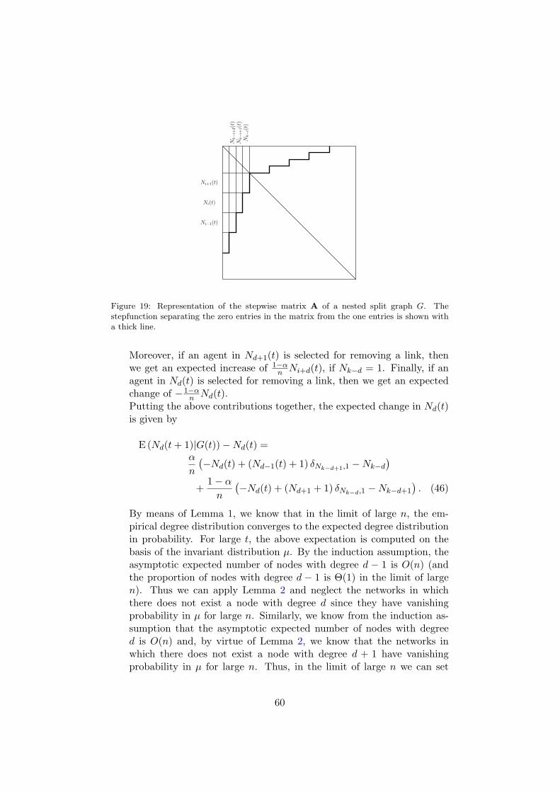
Ni−1(t)
Ni(t)
Ni+1(t)
Nk−
i+2(t
)N
k−
i+1(t
)N
k−
i(t)
Figure 19: Representation of the stepwise matrix A of a nested split graph G. Thestepfunction separating the zero entries in the matrix from the one entries is shown witha thick line.
Moreover, if an agent in Nd+1(t) is selected for removing a link, thenwe get an expected increase of 1−α
n Ni+d(t), if Nk−d = 1. Finally, if anagent in Nd(t) is selected for removing a link, then we get an expectedchange of −1−α
n Nd(t).Putting the above contributions together, the expected change in Nd(t)is given by
E (Nd(t + 1)|G(t)) − Nd(t) =α
n
(
−Nd(t) + (Nd−1(t) + 1) δNk−d+1,1 − Nk−d
)
+1 − α
n
(
−Nd(t) + (Nd+1 + 1) δNk−d,1 − Nk−d+1
)
. (46)
By means of Lemma 1, we know that in the limit of large n, the em-pirical degree distribution converges to the expected degree distributionin probability. For large t, the above expectation is computed on thebasis of the invariant distribution µ. By the induction assumption, theasymptotic expected number of nodes with degree d − 1 is O(n) (andthe proportion of nodes with degree d − 1 is Θ(1) in the limit of largen). Thus we can apply Lemma 2 and neglect the networks in whichthere does not exist a node with degree d since they have vanishingprobability in µ for large n. Similarly, we know from the induction as-sumption that the asymptotic expected number of nodes with degreed is O(n) and, by virtue of Lemma 2, we know that the networks inwhich there does not exist a node with degree d + 1 have vanishingprobability in µ for large n. Thus, in the limit of large n we can set
60
limt→∞ δNk−d+1(t),1 = limt→∞ δNk−d(t),1 = 1, since the existence of nodeswith degrees d and d + 1 imply that Nk−d+1 = Nk−d = 1. Denoting bynd the asymptotic expected proportion of nodes with degree d , we getfrom Equation (46) the following relationship
nd = αnd−1 + (1 − α)nd+1. (47)
Since by assumption nd−1 and nd are Θ(1) for increasing n, Equation(47) shows that this also holds for nd+1. This proves the inductionstep.42
The above discussion allows us to derive a recursive relationship for theexpected degree distribution in the limit of large n and t. From Equations(47) and (45) we get
nd =1 − α
αnd+1 +
1 − 2α
αn, (48)
for all 0 ≤ d < d∗. From Lemma 3 we know that n0 = n+α−2nα(1−α)n . The
solution of the recurrence Equation (48) is then given by
nd =1 + n − 2nα
(1 − α)n
(
1 − α
α
)d
. (49)
Moreover, we have that the sum of the sizes of the sets must be equal tothe total number of agents, n. We know that the number of agents in thedominating sets with degrees larger than d∗ is d∗ (since each set containsonly one node and there are d∗ such sets).43 Adding this to the number ofagents in the independent sets with degree d = 0, ..., d∗ yields
d∗∑
d=0
nd = n − d∗
n. (50)
Further, inserting Equation (49) in Equation (50) we can derive the numberd∗ of independent sets as a function of n and α
d∗(n, α) =ln(
2(1−α)1+n−2nα
)
ln(
α1−α
) . (51)
42Note that for the degrees larger than d∗ this iterative procedure does not hold anymore since the number of nodes with a degree larger than d∗ is at most one.
43Note that since those networks in which there does not exist a node with degree0 ≤ d ≤ d∗ in the corresponding independent set can be neglected, the structure of nestedsplit graphs implies that all dominating sets have size one.
61
d∗ is a monotonic decreasing function of nd∗ with the limits limα→0 d∗ = 0and limα→1/2 d∗ = n−1
2 . This completes the proof. 2
Proof of Corollary 4. Note that for all agents in the independent sets,u ∈ Di with 1 ≤ i ≤
⌊
k2
⌋
, the clustering coefficient is one, since theirneighbors are all connected among each other. Next, we consider the agentsu ∈ Di with
⌊
k2
⌋
+ 1 ≤ i ≤ k and degree du =∑i
j=1 |Dk+1−j | − 1. Theneighbors of agent u that form a clique are all connected among each other
with a total of 12
(
∑kj=⌊ k
2⌋+1|Dj | − 1
)(
∑kj=⌊ k
2⌋+1|Dj | − 2
)
links, excluding
agent u from the clique. The neighbors of u in the independent sets are notconnected. Finally, we consider the links between neighbors for which oneneighbor is in a clique and one neighbor is in an independent set. If k is
even we get∑⌊ k
2⌋j=k−i+1 |Dj |
(
∑kl=k−j+1 |Dl| − 1
)
links, excluding agent u in
the clique (see Figure 11 (left)). If k is odd there is no such contributionfor the agents in the set D⌊ k
2⌋+1 (see Figure 11 (right)). Putting these
contributions together we obtain the clustering coefficient if an agent u ∈ Di
for all i = 1, ..., k. 2
Proof of Corollary 5. First, consider an agent u ∈ Di with i = 1, ...,⌊
k2
⌋
corresponding to the independent sets. We know that the number of neigh-bors (degree) of agent u is given by
∑ij=1 |Dk+1−j |. The neighbors of
agent u are the agents in the cliques with degrees given in Equation (14).Thus, the number of neighbors of the neighbors of u in the sets Dk+1−j is∑k+1−j
l=1 |Dk+1−l| − 1. Putting the above results together, we obtain for thenearest neighbor connectivity of agent u the following expression.
dnn(u) =1
∑ij=1 |Dk+1−j |
i∑
j=1
|Dk+1−j |(
k+1−j∑
l=1
|Dk+1−l| − 1
)
(52)
for u ∈ Di, i = 1, ...,⌊
k2
⌋
.
Next we consider an agent u in the set Di with⌊
k2
⌋
+ 1 ≤ i ≤ k cor-responding to the cliques. The number of neighbors of agent u is givenby∑i
j=1 |Dk+1−j | − 1. The number of neighbors of an agent v ∈ Dj ,⌊
k2
⌋
+ 1 ≤ j ≤ k in the cliques is given by∑j
l=1 |Dk+1−l| − 1. Since agent uis connected to all agents in the cliques we can sum over all their neighbor-
hoods with a total of∑k
j=⌊ k2⌋+1
|Dj |(
∑jl=1 |Dk+1−l| − 1
)
neighbors. The
number of neighbors of agent w ∈ Dj , 1 ≤ j ≤⌊
k2
⌋
in the independent sets is
given by∑j
l=1 |Dk+1−l|. If k is even then agent u is connected to all agentsin the independent sets from the level k − i + 1 to
⌊
k2
⌋
yielding a total of∑⌊ k
2⌋j=k−i+1 |Dj |
∑jl=1 |Dk+1−l| neighbors (see Figure 11). Thus, the nearest
62
neighbor connectivity of agent u is given by
dnn(u) = 1∑i
j=1 |Dk+1−j |−1
[
∑kj=⌊ k
2⌋+1|Dj |
(
∑jl=1 |Dk+1−l| − 1
)
+∑⌊ k
2⌋j=k−i+1 |Dj |
∑jl=1 |Dk+1−l|
] (53)
for u ∈ Di with 1 ≤ i ≤⌊
k2
⌋
. If k is odd, then the agents in the independentsets to not contribute to the neighbors of the agents in the set D⌊ k
2⌋+1 (see
Figure 11) and we can neglect the second term in the above equation. 2
Proof of Corollary 6. We first consider all pairs of agents in the cliques.All theses agents are adjacent to each other and thus the shortest path be-
tween them has length one. Moreover, there are 12
∑kj=⌊ k
2⌋+1|Dj |
(
∑kj=⌊ k
2⌋+1|Dj | − 1
)
pairs of agents in the cliques.Next, we consider all pairs of agents in the independent sets. From Equa-
tion (56) we know that all of them are at a distance of two links separated
from each other. Moreover, there are 12
∑⌊ k2⌋
j=1 |Dj |(
∑⌊ k2⌋
j=1 |Dj | − 1
)
pairs
of agents in which both agents stem from an independent set.Now we consider the pairs of agents in which one agent is in the in-
dependent set D1. Then there are |D1||Dk| pairs of agents with short-
est path 1 and |D1|(
∑k−1j=1 |Dj | − 1
)
pairs of agents with shortest path 2.
Similarly, we can consider the pairs in which one agent is in the set D2.Then we have |D2|(|Dk| + |Dk−1|) pairs of agents with shortest path 1 and
|D2|(
∑k−2j=1 |Dj | − 1
)
pairs of agents with shortest path 2. Finally, if one
agent is in the set D⌊ k2⌋ then we have |D⌊ k
2⌋|∑k
j=⌊ k2⌋+1
|Dj | pairs of agents
with distance 1 and |D⌊ k2⌋|(
∑⌊ k2⌋
j=1 |Dj | − 1
)
pairs with distance 2, if k is
even (see Figure 11 (left)). If k is odd (see Figure 11 (right)), we have andone agent is in the set D⌊ k
2⌋ then we have |D⌊ k2⌋|∑k
j=⌊ k2⌋+2
|Dj | pairs of
agents with distance 1 and |D⌊ k2⌋|(
∑⌊ k2⌋+1
j=1 |Dj | − 1
)
pairs with distance
2 (see Figure 11). Similarly, all agents in the independent sets Di with1 ≤ i ≤
⌊
k2
⌋
can be considered.Therefore, assuming that k is even, the average path length L defined in
63
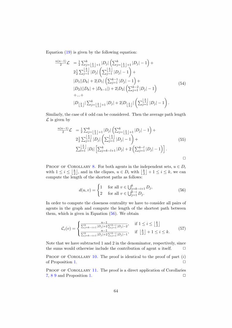
Equation (19) is given by the following equation:
n(n−1)2 L = 1
2
∑kj=⌊ k
2⌋+1|Dj |
(
∑kj=⌊ k
2⌋+1|Dj | − 1
)
+
212
∑⌊ k2⌋
j=1 |Dj |(
∑⌊ k2⌋
j=1 |Dj | − 1
)
+
|D1||Dk| + 2|D1|(
∑k−1j=1 |Dj | − 1
)
+
|D2|(|Dk| + |Dk−1|) + 2|D2|(
∑k−2j=1 |Dj | − 1
)
+...+
|D⌊ k2⌋|∑k
j=⌊ k2⌋+1
|Dj | + 2|D⌊ k2⌋|(
∑⌊ k2⌋
j=1 |Dj | − 1
)
.
(54)
Similarly, the case of k odd can be considered. Then the average path lengthL is given by
n(n−1)2 L = 1
2
∑kj=⌊ k
2⌋+1|Dj |
(
∑kj=⌊ k
2⌋+1|Dj | − 1
)
+
212
∑⌊ k2⌋
j=1 |Dj |(
∑⌊ k2⌋
j=1 |Dj | − 1
)
+
∑⌊ k2⌋
l=1 |Dl|[
∑kj=k−l+1 |Dj | + 2
(
∑k−lj=1 |Dj | − 1
)]
.
(55)
2
Proof of Corollary 8. For both agents in the independent sets, u ∈ Di
with 1 ≤ i ≤⌊
k2
⌋
, and in the cliques, u ∈ Di with⌊
k2
⌋
+ 1 ≤ i ≤ k, we cancompute the length of the shortest paths as follows:
d(u, v) =
1 for all v ∈ ⋃kj=k−i+1 Dj ,
2 for all v ∈ ⋃k−ij=1 Dj .
(56)
In order to compute the closeness centrality we have to consider all pairs ofagents in the graph and compute the length of the shortest path betweenthem, which is given in Equation (56). We obtain
Cc(v) =
n−1∑k
j=k−i+1 |Dj |+2∑k−i
j=1 |Dj |−2, if 1 ≤ i ≤
⌊
k2
⌋
n−1∑k
j=k−i+1 |Dj |+2∑k−i
j=1 |Dj |−1, if
⌊
k2
⌋
+ 1 ≤ i ≤ k.(57)
Note that we have subtracted 1 and 2 in the denominator, respectively, sincethe sums would otherwise include the contribution of agent u itself. 2
Proof of Corollary 10. The proof is identical to the proof of part (i)of Proposition 1. 2
Proof of Corollary 11. The proof is a direct application of Corollaries7, 8 9 and Proposition 1. 2
64


![Introducing Serendipity in a Social Network Model of ... · model the process of learning in an agent-based network. In Gale and Kariv model of social learning [14], the process of](https://img.pdfslide.us/doc/110x75/60378725b25d0e35617f6e61/introducing-serendipity-in-a-social-network-model-of-model-the-process-of-learning.jpg)