Embed Size (px)
Citation preview
A Dynamic Framework for Intelligent Control of River Flooding -A Case Study
Arturo S. Leon, P.E., M.ASCE1, Elizabeth A. Kanashiro2,Rachelle Valverde3 and Venkataramana Sridhar, P.E., M.ASCE4
ABSTRACT
This paper presents a case study on the application of a dynamic framework for the intelli-
gent control of flooding in the Boise River system in Idaho. This framework couples a robust
and numerically efficient hydraulic routing approach with the popular multi-objective Non-
dominated Sorting Genetic Algorithm II (NSGA-II). The novelty of this framework is that it
allows for controlled flooding when the conveyance capacity of the river system is exceeded
or is about to exceed. Controlled flooding is based on weight factors assigned to each reach of
the system depending on the amount of damage that would occur, should a flood occur. For
example, an urban setting would receive a higher weight factor than a rural or agricultural area.
The weight factor for a reach doesn’t need to be constant as it can be made a function of the
flooding volume (or water stage) in the reach. The optimization algorithm minimizes flood
damage by favoring low weighted floodplain areas (e.g., rural areas) rather than high weighted
areas (e.g., urban areas) for the overbank flows. The proposed framework has the potential to
1Assistant Professor, School of Civil and Construction Engineering, Oregon State University, 220Owen Hall, Corvallis, OR 97331-3212, USA. E-mail: [email protected] (Correspondingauthor)
2Hydraulic Engineer, Ausenco-Vector, Calle Esquilache 371, San Isidro, Lima - Peru. E-mail:[email protected]
3Graduate Research Assistant, School of Civil and Construction Engineering, Oregon State Univer-sity, 220 Owen Hall, Corvallis, OR 97331, USA. E-mail: [email protected]
4Assistant Professor, Civil Engineering, Boise State University, 1910 University Drive, Boise, ID83725-2060, USA. E-mail: [email protected]
1
improve water management and use of flood-prone areas in river systems, especially of those
systems subjected to frequent flooding. This work is part of a long term project which aims
at developing a reservoir operation model that combines short-term objectives (e.g., flooding)
and long-term objectives (e.g., hydropower, irrigation, water supply). The scope of this first
paper is limited to the application of the proposed framework to flood control. Results for the
Boise River system show a promising outcome in the application of this framework for flood
control.
Keywords: Flooding; Genetic Algorithms; Hydraulic routing; Multi-objective Opti-
mization; Real-time control; Regulated river systems; River management; River oper-
ation
List of Figures
1 Flow chart of OSU Rivers . . . . . . . . . . . . . . . . . . . . . . . . 25
2 Cross-section schematic for definition of left and right flooding volumes. 26
3 An example of a Flooding Performance Graph (FPG) . . . . . . . . . 27
4 An example of a Rating performance Graph (RPG) . . . . . . . . . . 28
5 Schematic of a river reach . . . . . . . . . . . . . . . . . . . . . . . 29
6 Schematic of a node . . . . . . . . . . . . . . . . . . . . . . . . . . . 30
7 Schematic of the Boise River’s Plan View . . . . . . . . . . . . . . . 31
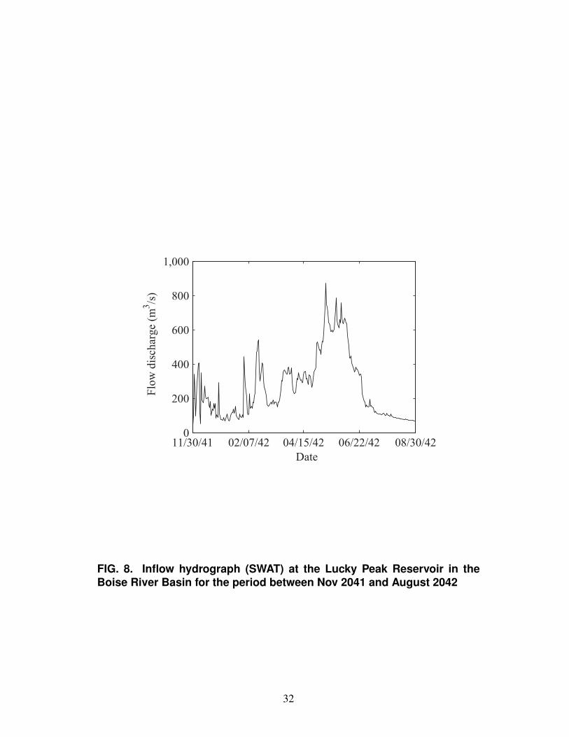
8 Inflow hydrograph (SWAT) at the Lucky Peak Reservoir in the Boise
River Basin for the period between Nov 2041 and August 2042 . . . . 32
9 Plan view of major storage reservoirs in the Boise River basin. . . . . 33
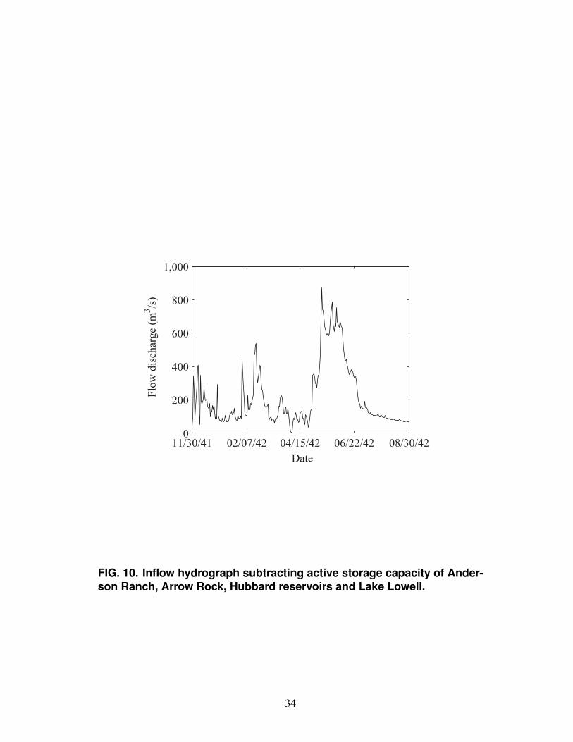
10 Inflow hydrograph subtracting active storage capacity of Anderson Ranch,
Arrow Rock, Hubbard reservoirs and Lake Lowell. . . . . . . . . . . 34
11 Stage-storage relationship of Lucky Peak reservoir. . . . . . . . . . . 35
12 Aerial view of Lucky Peak reservoir and associated structures (source:
http://commons.wikimedia.org) . . . . . . . . . . . . . . . . . . . . . 36
2

13 Rating curve at most downstream end of river system (node J26). . . . 37
14 Flow hydrographs at downstream end of reach R1 for simulated sce-
narios. . . . . . . . . . . . . . . . . . . . . . . . . . . . . . . . . . . 38
15 Flow hydrographs at downstream end of reach R10 for simulated sce-
narios. . . . . . . . . . . . . . . . . . . . . . . . . . . . . . . . . . . 39
16 Detail A in Figure 15. . . . . . . . . . . . . . . . . . . . . . . . . . . 40
17 Flow hydrographs at downstream end of reach R22 for simulated sce-
narios. . . . . . . . . . . . . . . . . . . . . . . . . . . . . . . . . . . 41
18 Stage hydrographs at downstream end of reach R1 for simulated sce-
narios. . . . . . . . . . . . . . . . . . . . . . . . . . . . . . . . . . . 42
19 Stage hydrographs at downstream end of reach R10 for simulated sce-
narios. . . . . . . . . . . . . . . . . . . . . . . . . . . . . . . . . . . 43
20 Detail B in Figure 19. . . . . . . . . . . . . . . . . . . . . . . . . . . 44
21 Stage hydrographs at downstream end of reach R22 for simulated sce-
narios. . . . . . . . . . . . . . . . . . . . . . . . . . . . . . . . . . . 45
22 Peak flow at downstream end of reaches R1, R10 and R22 for the sec-
ond scenario. . . . . . . . . . . . . . . . . . . . . . . . . . . . . . . 46
23 Flooding objective (Eq. 1) for simulated scenarios. . . . . . . . . . . 47
24 Inflow, outflow and water stage hydrographs at the Lucky Peak reservoir. 48
25 Gate operation traces (six gates) at the Lucky Peak reservoir according
to OSU Rivers . . . . . . . . . . . . . . . . . . . . . . . . . . . . . . 49
INTRODUCTION
River flooding is a recurrent threat that normally ensues a huge cost, both in terms
of human suffering and economic losses associated with damage to infrastructure, loss
of business, and the cost of insurance claims. From 2005 to 2009 the National Weather
Service (2009) estimated 63 billion dollars in losses in the U.S. associated with flood-
3
ing. The catastrophic disasters associated with river flooding urge the re-evaluation of
current strategies for flood control for most appropriate frameworks.
Recent studies on flood mitigation indicate that major emphasis must be given to
flood control projects under the greater framework of basin-wide ecosystem rehabil-
itation (e.g., United Nations Environment Programme 2003, De Bruijn et al. 2008).
These studies also aim for improving structural measures for minimizing the impact of
floods while emphasizing the importance of risk management in flood control projects.
A review of common structural measures used for flood control (e.g., levees, dams)
reveals most of these measures are passive (static), with dams being the most impor-
tant structural measure for flood control (e.g., Wei and Hsu 2008). Most dams built for
flood control have gates that are operated based on rule curves, which are determined
based on annual estimates of system loads, reservoir storages and resources provided
by stakeholders. Rule curves neglect the flow dynamics in the entire river system,
which makes this approach a “slow-response” method for flood control. This is partic-
ularly true in complex river systems when parts of the river system may have enough
in-line storage capacity, while other portions of the system may be overflowing.
A flooding process may be highly dynamic and may start from anywhere in the
river system (Leon and Kanashiro 2010). It may start from upstream (e.g., large in-
flows), downstream (i.e., high water levels at downstream), or laterally from the con-
necting reaches (e.g., water levels at river junctions near the reach banks). It may
change for the same river system depending on inflows to the river system and an-
tecedent boundary conditions. Accounting for system flow dynamics is also important
because flow conveyance from one reservoir to another is not instantaneous but de-
pends on the capacity of the connecting reaches, the capacity of associated gates, outlet
structures and the dynamic hydraulic gradients. Clearly, rule curves are insufficient for
making system-wide operational decisions.
4

Various models for reservoir operation are available. These include optimiza-
tion models, simulation models, and combined simulation-optimization models. For
achieving an optimal system-wide operational decision for flood control, it was rec-
ognized that optimization and simulation components must be combined (e.g., Hydro-
logic Engineering Center 2003). Within the category of models that combine simula-
tion and optimization, there are various models intended for reservoir operation includ-
ing flood control. One of these models is the “Generalized Real-Time Flood Control
System Model” (Eichert and Pabst 1998) that was developed by the Hydrologic En-
gineering Center (HEC). Currently, HEC supports three individual reservoir modeling
tools for the simulation and optimization of reservoir system operations (Hydrologic
Engineering Center 1996, 2003). The tools include: 1) Reservoir Simulation (HEC-
ResSim), 2) Multi-Objective Reservoir Optimization (Prescriptive Reservoir Model,
HEC-PRM), and 3) Reservoir Flood Control Optimization (HECFloodOpt). HEC-
ResSim is a reservoir simulation model that makes operation decisions following the
user specified operating rules or guidelines. HEC-PRM and HEC-FloodOpt are op-
timization models that make operation decisions to maximize system objectives and
values as defined by the user. HEC combines these three modeling tools into one
package, the Reservoir Evaluation System (HEC-RES). The simulation component of
HEC-RES, ResSim, is used extensively in real-time water control as part of the Corps
Water Management System (CWMS). The RIBASIM (RIver BAsin SIMulation) [Delft
Hydraulics 2000] model is another comprehensive and flexible tool for reservoir oper-
ation.
Recently, many more combined simulation-optimization models were formulated
for reservoir operation including flood control. Ngo et al. (2007) proposed to optimize
the control strategies for the Hoa Binh reservoir operation. The control strategies were
set up in the MIKE 11 simulation model to guide the releases of the reservoir system
5

according to the current storage level, the hydro-meteorological conditions, and the
time of the year. Lee et al. (2009) refined an existing optimization/simulation proce-
dure for rebalancing flood control and refill objectives for the Columbia River Basin for
anticipated global warming. To calibrate the optimization model for the 20th century
flow, the objective function was tuned to reproduce the current reliability of reservoir
refill, while providing comparable levels of flood control to those produced by current
flood control practices. After the optimization model was calibrated using the 20th
century flow the same objective function was used to develop flood control curves for
a global warming scenario.
Even though there is a wide array of models for reservoir operation, the authors
are not aware of any framework intended for the operation of a river system when its
capacity has exceeded or is about to exceed. Therefore, it would be desirable to have
a framework that allows controlled flooding, where areas with the lowest amount of
damage would be allowed to flood first and areas with the highest amount of damage
would be allowed to flood last to minimize damage accordingly.
This paper presents a case study on the application of a dynamic framework for
the intelligent control of flooding in the Boise River system in Idaho. This framework
that is under ongoing development was named OSU Rivers as an acronym for Oregon
State University coupled optimization-simulation model for the operation of regulated
river systems. The OSU Rivers framework couples a robust and numerically efficient
hydraulic routing approach with the popular multi-objective Non-dominated Sorting
Genetic Algorithm II (NSGA-II). The novelty of this framework is that it allows for
controlled flooding when the conveyance capacity of the river system is exceeded or is
about to exceed. Controlled flooding is based on weight factors assigned to each reach
of the system depending on the amount of damage that would occur, should a flood
occur. For example an urban setting would receive a higher weight factor than a rural
6
or agricultural area. The weight factor for a reach doesn’t need to be constant as it
can be made a function of the flooding volume (or water stage) in the reach. The opti-
mization algorithm minimizes flood damage by favoring low weighted floodplain areas
(e.g., rural areas) rather than high weighted areas (e.g., urban areas) for the overbank
flows. In an actual river system, presumably, rural areas are already more prone to
flooding (flood more frequently), because of existing planning and land management
practices. However, the proposed framework has the potential to refine and improve
water management and use of flood-prone areas in river systems, especially of those
systems subjected to frequent flooding.
The work presented here is part of a long term project, which overarching goal is
the development of a reservoir operation model that combines short-term objectives
(e.g., flooding) and long-term objectives (e.g., hydropower, irrigation, water supply).
The scope of this first paper is limited to the application of OSU Rivers to flood con-
trol (short-term objective). The treatment of long-term objectives will be described
in a subsequent paper. This paper is organized as follows: (1) the optimization and
simulation components of OSU Rivers are briefly described; (2) a concise description
of the river system routing of OSU Rivers is presented; (3) the model is applied to the
Boise River system in Idaho. Finally, the results are summarized in the conclusion.
COMPONENTS OF THE PROPOSED FRAMEWORK
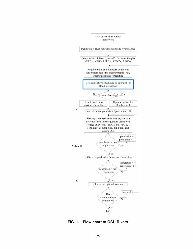
The proposed framework, the flow chart of which is presented in Figure 1, is es-
sentially a real-time operational model that links two components: optimization and
river system routing (simulation).
Optimization component: The Non-dominated Sorting Genetic Algorithm-II (NSGA-
II)
The optimization component of the OSU Rivers framework uses the popular Non-
dominated Sorting Genetic Algorithm-II (NSGA-II), which has been chosen based on
7
its recent successful implementation in reservoir optimization analysis (e.g., Kim et al.
2006). The NSGA-II algorithm has been shown to be one of the most efficient algo-
rithms for multi-objective optimization on a number of benchmark problems, including
water resources engineering problems (e.g., Bekele and Nicklow 2007). Some of the
recent applications to water resources engineering include multi-reservoir system opti-
mization (e.g., Kim et al. 2006), optimal design of water distribution networks (Atiquz-
zaman et al. 2006), long-term groundwater monitoring design (Reed and Minsker
2004), and watershed water quality management (Dorn and Ranji-Ranjithan 2003).
The main features of these algorithms are the implementation of a fast non-dominated
sorting procedure and its ability to handle multiple objectives simultaneously without
weight factors.
The reason for choosing a multi-objective optimization technique (i.e., NSGA-II) is
that, under non-flooding conditions, the OSU Rivers framework maximizes the benefits
of the river system that may be multi-objective such as hydropower production, irriga-
tion and water supply. Under flooding conditions, the OSU Rivers framework uses a
single-objective (minimize flooding), however to avoid using different algorithms, the
multi-objective NSGA-II technique is used for both flooding and non-flooding condi-
tions.
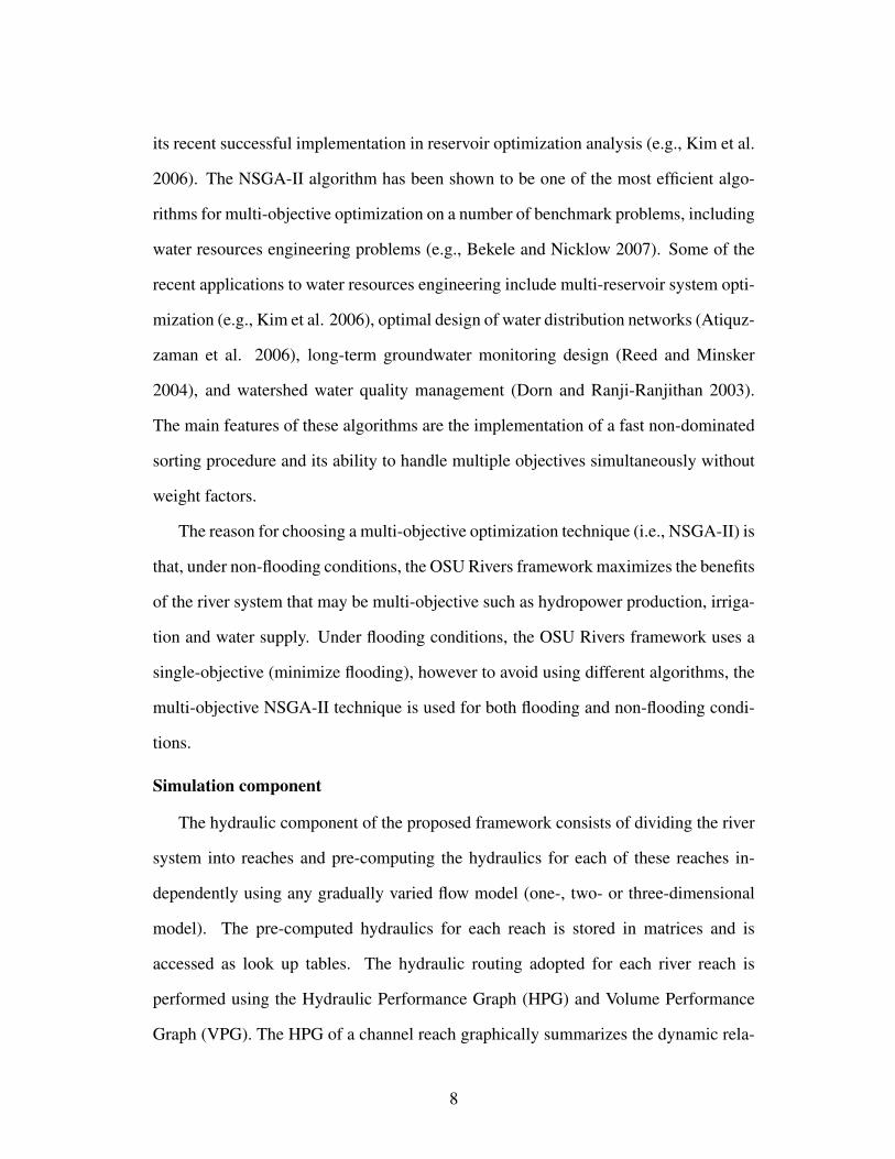
Simulation component
The hydraulic component of the proposed framework consists of dividing the river
system into reaches and pre-computing the hydraulics for each of these reaches in-
dependently using any gradually varied flow model (one-, two- or three-dimensional
model). The pre-computed hydraulics for each reach is stored in matrices and is
accessed as look up tables. The hydraulic routing adopted for each river reach is
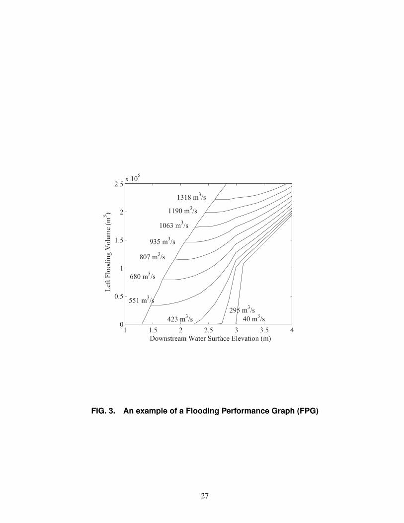
performed using the Hydraulic Performance Graph (HPG) and Volume Performance
Graph (VPG). The HPG of a channel reach graphically summarizes the dynamic rela-
8

tion between the flow through and the stages at the ends of the reach under gradually
varied flow (GVF) conditions, while the VPG summarizes the corresponding storage.
The storage volumes from VPGs are divided into left, right and main channel storages
volumes. The left and right inundation volumes are summarized into Left Flooding
Performance Graphs (LFPGs) and Right Flooding Performance Graphs (RFPGs), re-
spectively. The LFPGs and RFPGs represent volumes of water outside of levee limits,
channel banks or topographic thresholds that were used to define the limits of inunda-
tion (See Figure 2). An example of an LFPG is shown in Figure 3.
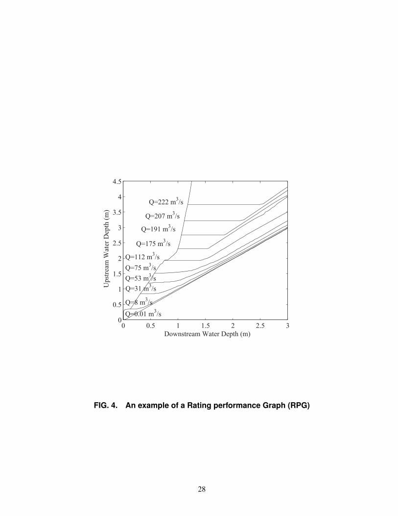
At the location of in-line structures (controlled and uncontrolled), the proposed
framework makes use of Rating Performance Graphs (RPGs). An RPG graphically
summarizes the dynamic relation between the flow through and the stages upstream
and downstream of an in-line structure under GVF conditions. Figure 4 depicts a typ-
ical graph of an RPG. Physical measurements of flow discharge and water stages or
numerical simulations using one-, two- or three-dimensional numerical models can be
used for constructing RPGs. In OSU Rivers, all internal nodes (uncontrolled and con-
trolled in-line structures and channel junctions) are assumed to have no storage. The
water depth immediately upstream of the in-line structure is computed using the RPG
constructed for the structure. For a detailed description of the hydraulic component of
the proposed framework the reader is referred to Leon et al. (2012).
Description of the proposed framework
For facilitating the description of OSU Rivers, this model can be divided into five
modules. These are:
Module I: Representation of a river network
In the proposed model, a river system is represented by river reaches and nodes.
A river reach is defined by its upstream and downstream nodes and must have more
or less uniform properties along the reach (e.g., cross-section, bed slope). The flow
9
direction in a river reach is assumed to be from its upstream node to its downstream
node as shown in Figure 5. A negative flow discharge in a river reach indicates that
reverse flow occurs in that river reach. In Figure 5, the subscript j and superscript
n represent the river reach index and the discrete-time index, respectively. Also, y is
water depth, Q is flow discharge and the subscripts u and d denote the upstream and
downstream ends of a river reach, respectively.
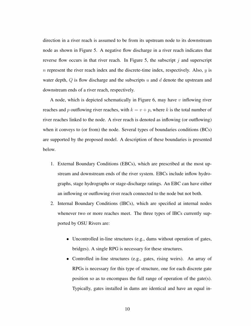
A node, which is depicted schematically in Figure 6, may have v inflowing river
reaches and p outflowing river reaches, with k = v + p, where k is the total number of
river reaches linked to the node. A river reach is denoted as inflowing (or outflowing)
when it conveys to (or from) the node. Several types of boundaries conditions (BCs)
are supported by the proposed model. A description of these boundaries is presented
below.
1. External Boundary Conditions (EBCs), which are prescribed at the most up-
stream and downstream ends of the river system. EBCs include inflow hydro-
graphs, stage hydrographs or stage-discharge ratings. An EBC can have either
an inflowing or outflowing river reach connected to the node but not both.
2. Internal Boundary Conditions (IBCs), which are specified at internal nodes
whenever two or more reaches meet. The three types of IBCs currently sup-
ported by OSU Rivers are:
• Uncontrolled in-line structures (e.g., dams without operation of gates,
bridges). A single RPG is necessary for these structures.
• Controlled in-line structures (e.g., gates, rising weirs). An array of
RPGs is necessary for this type of structure, one for each discrete gate
position so as to encompass the full range of operation of the gate(s).
Typically, gates installed in dams are identical and have an equal in-
10
vert elevation. For instance, if a dam has 10 identical gates that have
the same invert elevation, all gates have the same RPG, which reduces
drastically the number of RPGs needed for simulations.
• Junctions, which are schematically depicted in Figure 6, represent nodes
without presence of hydraulic structures. A junction node is assumed
not to have storage and may connect two or more river reaches.
Module II: Computation of HPGs, VPGs, LFPGs, RFPGs and RPGs
HPGs, VPGs, LFPGs, RFPGs are needed for all reaches of the river system, while
RPGs are needed for all uncontrolled and controlled in-line structures. The flow dis-
charges used for constructing the performance graphs should range from near dry-bed
states to high water stages (e.g., inundation) using appropriate intervals between flow
discharges. These intervals are set according to the desired precision by a trial and
error process.
Module III: Initial and Boundary Conditions
The initial conditions are downstream water depths and flow discharges at upstream
Qu and downstream Qd ends of each river reach. To check the consistency of initial
conditions, continuity equations and compatibility conditions of water stages are ver-
ified for all internal nodes. The boundary conditions are basically the inflows to the
river system and rating curves at the downstream ends of a river system. In OSU
Rivers, initial and boundary conditions can be continuously updated by real-time mea-
surements in the river system (e.g., water stages). The latter means that any error in
inflow discharge predictions at a previous time step will be minimized by real-time
measurements of water stages at the next time step (e.g., mass balance will be con-
served).
11
Module IV: Optimization objective under flooding conditions
Under flooding conditions, the following optimization objective is proposed
Minimize f =RR∑j=1
(wLjFVLj
+ wRjFVRj
) (1)
Where j denotes a river reach, RR is the total number of river reaches, and FVLj
and FVRjare left and right flooding volume, respectively (see Figure 2). FVLj
and
FVRjare obtained from the corresponding LFPG and RFPG, respectively. wL (or wR)
is a weight factor assigned to the left (or right) of each reach of the system depending
on the amount of damage that would occur, should the left (or right) of the reach
flood. In an actual application, weight factors should be determined from a social and
economic study based on a hierarchy of losses that would be incurred as a result of
flooding. It is worth mentioning that the weight factor for a reach doesn’t need to be
constant as it can be made a function of the flooding volume (or water stage) in the
reach.
Module V: River system hydraulic routing
This module assembles and solves a non-linear system of equations to perform the
hydraulic routing of the river system. These equations are assembled based on infor-
mation summarized in the systems’ HPGs, VPGs and RPGs, the reach-wise equation
of conservation of mass, continuity and compatibility conditions of water stages at the
union of reaches (nodes), and the system boundary conditions. For a detailed descrip-
tion of this hydraulic routing, the reader is referred to Leon et al. (2012).
APPLICATION OF THE PROPOSED MODEL TO THE BOISE RIVER
SYSTEM
For demonstration purposes, this model was applied to the Boise River system in
12
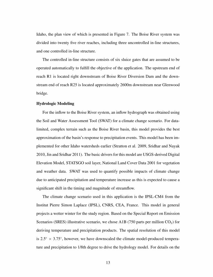
Idaho, the plan view of which is presented in Figure 7. The Boise River system was
divided into twenty five river reaches, including three uncontrolled in-line structures,
and one controlled in-line structure.
The controlled in-line structure consists of six sluice gates that are assumed to be
operated automatically to fulfill the objective of the application. The upstream end of
reach R1 is located right downstream of Boise River Diversion Dam and the down-
stream end of reach R25 is located approximately 2600m downstream near Glenwood
bridge.
Hydrologic Modeling
For the inflow to the Boise River system, an inflow hydrograph was obtained using
the Soil and Water Assessment Tool (SWAT) for a climate change scenario. For data-
limited, complex terrain such as the Boise River basin, this model provides the best
approximation of the basin’s response to precipitation events. This model has been im-
plemented for other Idaho watersheds earlier (Stratton et al. 2009, Sridhar and Nayak
2010, Jin and Sridhar 2011). The basic drivers for this model are USGS-derived Digital
Elevation Model, STATSGO soil layer, National Land Cover Data 2001 for vegetation
and weather data. SWAT was used to quantify possible impacts of climate change
due to anticipated precipitation and temperature increase as this is expected to cause a
significant shift in the timing and magnitude of streamflow.
The climate change scenario used in this application is the IPSL-CM4 from the
Institut Pierre Simon Laplace (IPSL), CNRS, CEA, France. This model in general
projects a wetter winter for the study region. Based on the Special Report on Emission
Scenarios (SRES) illustrative scenario, we chose A1B (750 parts per million CO2) for
deriving temperature and precipitation products. The spatial resolution of this model
is 2.5◦ × 3.75◦, however, we have downscaled the climate model-produced tempera-
ture and precipitation to 1/8th degree to drive the hydrology model. For details on the
13
downscaling and SWAT model simulation the readers are referred to Jin and Sridhar
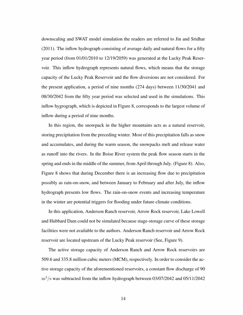
(2011). The inflow hydrograph consisting of average daily and natural flows for a fifty
year period (from 01/01/2010 to 12/19/2059) was generated at the Lucky Peak Reser-
voir. This inflow hydrograph represents natural flows, which means that the storage
capacity of the Lucky Peak Reservoir and the flow diversions are not considered. For
the present application, a period of nine months (274 days) between 11/30/2041 and
08/30/2042 from the fifty year period was selected and used in the simulations. This
inflow hygrograph, which is depicted in Figure 8, corresponds to the largest volume of
inflow during a period of nine months.
In this region, the snowpack in the higher mountains acts as a natural reservoir,
storing precipitation from the preceding winter. Most of this precipitation falls as snow
and accumulates, and during the warm season, the snowpacks melt and release water
as runoff into the rivers. In the Boise River system the peak flow season starts in the
spring and ends in the middle of the summer, from April through July. (Figure 8). Also,
Figure 8 shows that during December there is an increasing flow due to precipitation
possibly as rain-on-snow, and between January to February and after July, the inflow
hydrograph presents low flows. The rain-on-snow events and increasing temperature
in the winter are potential triggers for flooding under future climate conditions.
In this application, Anderson Ranch reservoir, Arrow Rock reservoir, Lake Lowell
and Hubbard Dam could not be simulated because stage-storage curve of these storage
facilities were not available to the authors. Anderson Ranch reservoir and Arrow Rock
reservoir are located upstream of the Lucky Peak reservoir (See, Figure 9).
The active storage capacity of Anderson Ranch and Arrow Rock reservoirs are
509.6 and 335.8 million cubic meters (MCM), respectively. In order to consider the ac-
tive storage capacity of the aforementioned reservoirs, a constant flow discharge of 90
m3/s was subtracted from the inflow hydrograph between 03/07/2042 and 05/11/2042
14
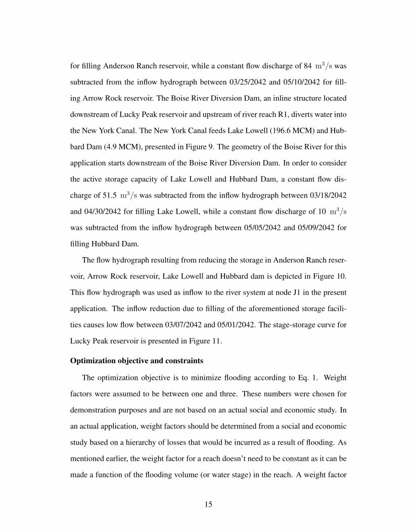
for filling Anderson Ranch reservoir, while a constant flow discharge of 84 m3/s was
subtracted from the inflow hydrograph between 03/25/2042 and 05/10/2042 for fill-
ing Arrow Rock reservoir. The Boise River Diversion Dam, an inline structure located
downstream of Lucky Peak reservoir and upstream of river reach R1, diverts water into
the New York Canal. The New York Canal feeds Lake Lowell (196.6 MCM) and Hub-
bard Dam (4.9 MCM), presented in Figure 9. The geometry of the Boise River for this
application starts downstream of the Boise River Diversion Dam. In order to consider
the active storage capacity of Lake Lowell and Hubbard Dam, a constant flow dis-
charge of 51.5 m3/s was subtracted from the inflow hydrograph between 03/18/2042
and 04/30/2042 for filling Lake Lowell, while a constant flow discharge of 10 m3/s
was subtracted from the inflow hydrograph between 05/05/2042 and 05/09/2042 for
filling Hubbard Dam.
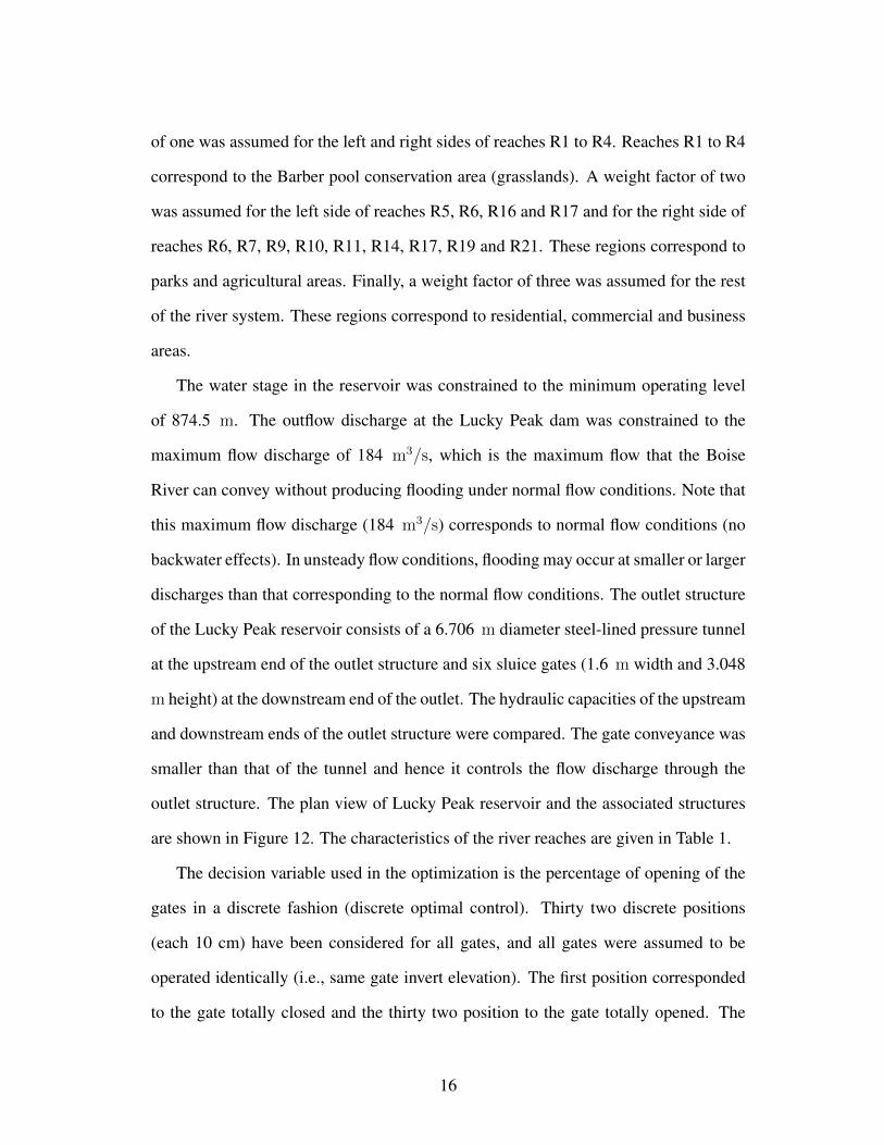
The flow hydrograph resulting from reducing the storage in Anderson Ranch reser-
voir, Arrow Rock reservoir, Lake Lowell and Hubbard dam is depicted in Figure 10.
This flow hydrograph was used as inflow to the river system at node J1 in the present
application. The inflow reduction due to filling of the aforementioned storage facili-
ties causes low flow between 03/07/2042 and 05/01/2042. The stage-storage curve for
Lucky Peak reservoir is presented in Figure 11.
Optimization objective and constraints
The optimization objective is to minimize flooding according to Eq. 1. Weight
factors were assumed to be between one and three. These numbers were chosen for
demonstration purposes and are not based on an actual social and economic study. In
an actual application, weight factors should be determined from a social and economic
study based on a hierarchy of losses that would be incurred as a result of flooding. As
mentioned earlier, the weight factor for a reach doesn’t need to be constant as it can be
made a function of the flooding volume (or water stage) in the reach. A weight factor
15
of one was assumed for the left and right sides of reaches R1 to R4. Reaches R1 to R4
correspond to the Barber pool conservation area (grasslands). A weight factor of two
was assumed for the left side of reaches R5, R6, R16 and R17 and for the right side of
reaches R6, R7, R9, R10, R11, R14, R17, R19 and R21. These regions correspond to
parks and agricultural areas. Finally, a weight factor of three was assumed for the rest
of the river system. These regions correspond to residential, commercial and business
areas.
The water stage in the reservoir was constrained to the minimum operating level
of 874.5 m. The outflow discharge at the Lucky Peak dam was constrained to the
maximum flow discharge of 184 m3/s, which is the maximum flow that the Boise
River can convey without producing flooding under normal flow conditions. Note that
this maximum flow discharge (184 m3/s) corresponds to normal flow conditions (no
backwater effects). In unsteady flow conditions, flooding may occur at smaller or larger
discharges than that corresponding to the normal flow conditions. The outlet structure
of the Lucky Peak reservoir consists of a 6.706 m diameter steel-lined pressure tunnel
at the upstream end of the outlet structure and six sluice gates (1.6 m width and 3.048
m height) at the downstream end of the outlet. The hydraulic capacities of the upstream
and downstream ends of the outlet structure were compared. The gate conveyance was
smaller than that of the tunnel and hence it controls the flow discharge through the
outlet structure. The plan view of Lucky Peak reservoir and the associated structures
are shown in Figure 12. The characteristics of the river reaches are given in Table 1.
The decision variable used in the optimization is the percentage of opening of the
gates in a discrete fashion (discrete optimal control). Thirty two discrete positions
(each 10 cm) have been considered for all gates, and all gates were assumed to be
operated identically (i.e., same gate invert elevation). The first position corresponded
to the gate totally closed and the thirty two position to the gate totally opened. The
16
use of the opening of the gates as decision variable can be justified in this application
because all gates were identical and they were assumed to be operated identically.
However, when the inline structure has different controlled hydraulic structures (e.g.,
gates having different invert elevations), the total flow discharge at the inline structure
rather than the percentage of opening of the gates should be used as decision variable.
Once the optimized value of the flow discharge at the inline structure is determined,
the RPG at the inline structure can be used for determining a combination of gates
that satisfy this optimized flow discharge. Clearly, multiple combinations of gates may
provide the same flow discharge
Initial and boundary conditions
The system under consideration has two external boundary conditions (EBCs): the
first BC is an inflow hydrograph at the upstream end of the Lucky Peak reservoir (see
Figure 10) and the second BC is a flow-stage relation at the downstream end of the last
river reach (see Figure 13). This flow-stage relation was built assuming critical flow
conditions. The initial conditions are a constant flow discharge in the system of 166.7
m3/s and a water stage in the Lucky Peak reservoir of 879.84 m. The simulation time
step and the operational decision time used were one hour.
Three scenarios were simulated. The first scenario is with no gate operation, i.e.
the gates are closed. The second scenario assumes that the Lucky Peak reservoir does
not exist. The third scenario operates the gates according to the results of the proposed
framework (minimizing the objective function presented in Eq. 1).
Results and analysis of scenarios
The simulated results for flow and stage hydrographs for the three scenarios under
consideration are presented in Figures 14 to 17 and 18 to 21, respectively. Reaches
R1, R10 and R22 are located at upstream, downstream and midway of the system (see
Figure 7), respectively. In the first scenario the gates remain closed and hence the
17
reservoir is rapidly filled. As expected, when the reservoir is full, the flow hydrograph
downstream of the reservoir (flow over the spillway) is similar to that of the second
scenario (no reservoir). The third scenario provides a better control of flooding, how-
ever flooding is not entirely avoided due to storage limitations. Figures 16 and 20 show
a zoom-in of regions A and B in Figures 15 and 19 (reach R10), respectively.
To estimate the flood attenuation by the Boise River downstream of Lucky peak
reservoir, an enlarged view of peak flows at the downstream ends of reaches R1, R10
and R22 for the second scenario (no reservoir) is presented in Figure 22. The inflow
hydrograph is also shown in Figure 22. As can be observed, the peak flow arrives to the
downstream end of reaches R1, R10 and R22 after one, three and seven hours, respec-
tively. The attenuation of the peak inflow hydrograph was calculated to be 2.41 m3/s
(0.28%), 3.87 m3/s (0.44%) and 6.35 m3/s (0.73%) when the peak flow arrives at the
downstream end of reaches R1, R10 and R22, respectively (see Figure 22). This small
attenuation is because the storage capacity of the Boise River system downstream of
Lucky peak reservoir is very small. The storage capacity of Boise River downstream of
the reservoir is about 0.7% of the maximum storage capacity of Lucky peak reservoir.
The simulated results of the flooding objective (Eq. 1) are shown in Figure 23.
Results of flooding volume and objective function 1 show that the river starts to flood
at day 16 for the first scenario, at day 2 for the second scenario and at day 165 for the
third scenario. Note that for the simulated inflow hydrograph, the Boise River would
flood for all scenarios. The operation of gates according to the proposed framework
(third scenario) attenuates and delays the flood but does not avoid flooding due to
lack of sufficient storage capacity. The storage capacity needed to avoid flooding for
the inflow hydrograph under consideration is 1,323 MCM. This means that another
reservoir with a capacity similar to that of Lucky peak reservoir (about 600 MCM)
would be necessary to avoid flooding in this case.
18
Results for optimized outflow discharges and water stages at the Lucky Peak reser-
voir according to the proposed framework (third scenario) are presented in Figure 24.
Figure 25 shows the corresponding trace of gate openings.
For the third scenario, before the reservoir is full, operated gates release a flow dis-
charge lower than 184 m3/s, which is the maximum flow discharge without flooding
under normal flow conditions. When the reservoir is full, the flow hydrograph is simi-
lar to the inflow hydrograph. The third scenario delayed and better controlled flooding;
however, flooding is not entirely avoided due to storage limitations.
CONCLUSIONS
This paper presents a dynamic framework for the intelligent control of river flood-
ing. The novelty of this framework is that it allows for controlled flooding when
the conveyance capacity of the river system is exceeded or is about to exceed. The
proposed approach links two components: river system routing (simulation) and op-
timization. The river system routing (simulation) component builds upon the appli-
cation of Performance Graphs, while the optimization component uses the popular
second generation multi-objective evolutionary algorithm Non-dominated Sorting Ge-
netic Algorithm-II (NSGA-II). For illustration purposes, the proposed framework was
applied to the Boise River system in Idaho. The key findings are as follows:
1. Results show that the Boise River would flood for all scenarios for the simu-
lated inflow hydrograph. The operation of controlled in-line structures accord-
ing to the results of the proposed framework delays the occurrence of flooding,
but does not avoid it due to lack of sufficient storage capacity in the reservoir.
2. The use of performance graphs for river system routing results in a robust and
numerically efficient model as most of the computations for the system routing
only involves interpolation steps.
19
3. Overall, the results show a promising outcome in the application of this model
for flood control.
ACKNOWLEDGMENTS
The authors gratefully acknowledge the financial support of NSF Idaho EPSCoR
Program and the National Science Foundation under award number EPS-0814387. The
first author would like to thank the financial support of the School of Civil and Con-
struction Engineering at Oregon State University. The first author would also like to
thank Mrs. Carmen Bernedo of MWH Americas for providing insightful comments
during the preparation of the manuscript. The last author would also like to acknowl-
edge the partial support that came from NOAA via the Pacific Northwest Climate Im-
pacts Research Consortium under award number NA10OAR4310218. Last but not
least, the authors are indebted to the anonymous reviewers for their insight, construc-
tive criticisms and suggestions on an earlier version of the manuscript.
REFERENCES
Atiquzzaman, M., Liong, S., and Yu, X. (2006). “Alternative decision making in wa-
ter distribution network with NSGA-II.” Journal of Water Resources Planning and
Management, 132(2), 122–126.
Bekele, E. G. and Nicklow, J. W. (2007). “Multi-objective automatic calibration of
SWAT using NSGA-II.” Journal of Hydrology, 341(3-4), 165 – 176.
De Bruijn, K. and Klijn, F. and Mcgahey, C. and Mens, M. and Wolfert, H. (2008).
“Long-term strategies for flood risk management: scenario definition and strategic
alternative design.” FLOODsite report T14-07-02 Deltares, Delft Hydraulics, Delft,
The Netherlands.
Delft Hydraulics (2000). RIBASIM user’s manual and technical reference manual.
Delft Hydraulics, Delft, The Netherlands.
20
Dorn, J. L. and Ranji-Ranjithan, S. (2003). “Evolutionary multi-objective optimization
in watershed water quality management.” EMO, 692–706.
Eichert, B. S. and Pabst, A. F. (1998). Generalized Real-Time Flood Control System
Model. U.S. Army Corps of Engineers, Davis, California.
Hydrologic Engineering Center (1996). “Developing seasonal and long-term reservoir
system operation plans using HEC-PRM.” Report RD-40, U.S. Army Corps of En-
gineers, Davis, California, USA.
Hydrologic Engineering Center (2003). Hydrologic Engineering Center’s Prescriptive
Reservoir Model, Program Description. U.S. Army Corps of Engineers, Davis, Cal-
ifornia, USA.
Jin, X. and Sridhar, V. (2011). “Impacts of climate change on hydrology and water
resources in the Boise and Spokane River Basins.” Journal of American Water Re-
sources Association, (in press).
Kim, T., Heo, J.-H., and Jeong, C.-S. (2006). “Multireservoir system optimization in
the Han River basin using multi-objective genetic algorithms.” Hydrol. Process., 20,
2057 – 2075.
Lee, S.-Y., Hamlet, A. F., Fitzgerald, C. J., and Burges, S. J. (2009). “Optimized Flood
Control in the Columbia River Basin for a Global Warming Scenario.” Journal of
Water Resources Planning and Management, 135(6), 440–450.
Leon, A. S. and Kanashiro, E. (2010). “A new coupled optimization-hydraulic routing
model for real-time operation of highly complex regulated river systems.” Presented
in the 2010 Watershed Management Conference: Innovations in Watershed Man-
agement Under Land Use and Climate Change.
Leon, A. S., Kanashiro, E. A., and Gonzalez-Castro, J. A. (2012). “A fast approach for
unsteady flow routing in complex river networks.” J. Hydraul. Eng., Under review.
National Weather Service (2009). “Flood losses: Compilation of flood loss statistics”,
21

<http://www.weather.gov/hic/flood stats/Flood loss time series.shtml>.
Ngo, L. L., Madsen, H., and Rosbjerg, D. (2007). “Simulation and optimization mod-
elling approach for operation of the Hoa Binh reservoir, Vietnam.” Journal of Hy-
drology, 336(34), 269 – 281.
Reed, P. M. and Minsker, B. S. (2004). “Striking the balance: Long-term groundwater
monitoring design for conflicting objectives.” Journal of Water Resources Planning
and Management, 130(2), 140–149.
Sridhar, V. and Nayak, A. (2010). “Implications of climate-driven variability and
trends for the hydrologic assessment of the Reynolds Creek Experimental Water-
shed, Idaho.” Journal of Hydrology, 385(1-4), 183 – 202.
Stratton, B. T., Sridhar, V., Gribb, M. M., McNamara, J. P., and Narasimhan, B. (2009).
“Modeling the spatially varying water balance processes in a semiarid mountain-
ous watershed of Idaho.” Journal of the American Water Resources Association, 45,
1390–1408 10.1111/j.1752-1688.2009.00371.x.
United Nations Environment Programme (2003). “Taking it at the flood”,
<http://www.unep.org/ourplanet/imgversn/141/shu.html>.
Wei, C.-C. and Hsu, N.-S. (2008). “Multireservoir flood-control optimization with
neural-based linear channel level routing under tidal effects.” Water Resources Man-
agement, 22, 1625–1647 10.1007/s11269-008-9246-8.
22
NOTATION
The following symbols are used in this paper:
EBC = external boundary condition;
c = average gravity wave celerity;
HPG = hydraulic performance graph;
I = inflow;
∀i = for all i;
N = set of nodes;
NB = set of downstream boundary nodes;
NS = set of source nodes;
O = outflow;
Qdj = flow discharge at downstream end of reach j;
Quj= flow discharge at upstream end of reach j;
S = storage;
u = average reach velocity;
VPG = volume performance graph;
∆x = length of river reach;
ydj = water depth at downstream end of reach j;
yuj= water depth at upstream end of reach j;
zdj = channel bottom elevation at downstream end of reach j;
zuj= channel bottom elevation at upstream end of reach j;
∆t = time stepSubscripts
d = downstream end index;
i = node index;
j = river reach index;
u = upstream end index
23

Superscripts
n = discrete-time index
24
Acquire initial and boundaryrr conditions(BCs) frff om real-time measurements (e.g.,
water stages) and foff recasting
Acquire initial and boundary conditions(BCs) from real-time measurements (e.g.,
water stages) and forecasting
population =population + 1population =population + 1
NSGA-II reprodudd ction / crossover / mutationNSGA-II reproduction / crossover / mutation
iver system hydraulic routing: solve asystem of non-linear equations assembled
based on systems’ HPG’s and VPG’s,continuity, compatibility conditions and
system BCs.
River system hydraulic routing: solve asystem of non-linear equations assembled
based on systems’ HPG’s and VPG’s,continuity, compatibility conditions and
system BCs.
EndEnd
generation =generation +1generation =generation +1
n = n +1n = n +1
population > maxpopulation
population > maxpopulation
generation > maxgeneration
generation > maxgeneration
Hassimulation beencompleted?
Hassimulation beencompleted?
Generate initial population (generation = 0)Generate initial population (generation = 0)
No
No
No
Yes
Choose the optimal solutionChoose the optimal solution
Yes
Yes
NSGA-II
Start of real-time controlfrff amework
Start of real-time controlframework
Defiff nition of river network: nodes and river reachesDefinition of river network: nodes and river reaches
Computation of River System Perfoff rmance Grapaa hs(HPG’s, VPG’s, LFPG’s, RFPG’s, RPG’s)
Computation of River System Performance Graphs(HPG’s, VPG’s, LFPG’s, RFPG’s, RPG’s)
Determine if system should be operated foff rflff ood foff recasting
Determine if system should be operated forflood forecasting
Prone to flff ooding?P g?Prone to flooding?
Operate system foff rflff ood control
Operate system forflood control
Operate system tomaximize benefiff tsOperate system tomaximize benefits
No Yes
FIG. 1. Flow chart of OSU Rivers
25
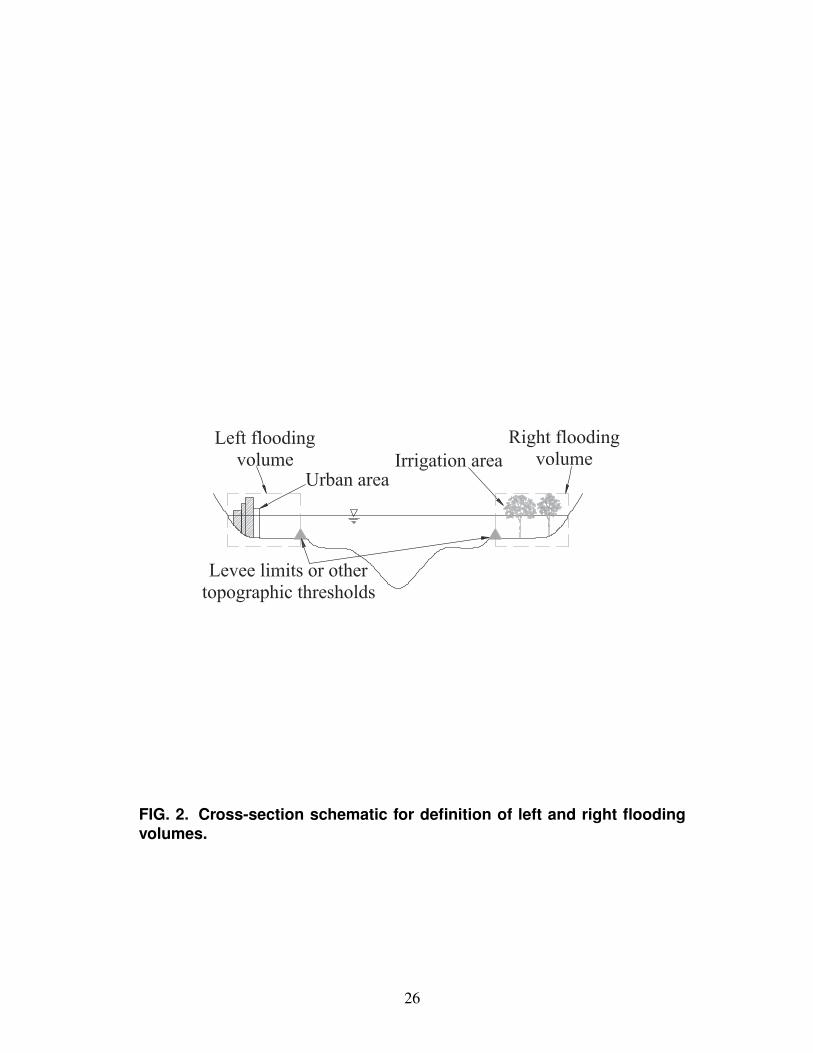
FIG. 2. Cross-section schematic for definition of left and right floodingvolumes.
26
1 1.5 2 2.5 3 3.5 40
0.5
1
1.5
2
2.5x 10⁵
Downstream Water Surface Elevation (m)
Lef
t Flo
odin
g V
olum
e (m
3 )
295 m3/s
680 m3/s
551 m3/s
40 m3/s
807 m3/s
935 m3/s
1063 m3/s
1190 m3/s
1318 m3/s
423 m3/s
FIG. 3. An example of a Flooding Performance Graph (FPG)
27
0 0.5 1 1.5 2 2.5 30
0.5
1
1.5
2
2.5
3
3.5
4
4.5
Downstream Water Depth (m)
Ups
tream
Wat
er D
epth
(m)
Q=0.01 m3/sQ=8 m3/s
Q=31 m3/sQ=53 m3/sQ=75 m3/sQ=112 m3/s
Q=191 m3/s
Q=175 m3/s
Q=207 m3/s
Q=222 m3/s
FIG. 4. An example of a Rating performance Graph (RPG)
28
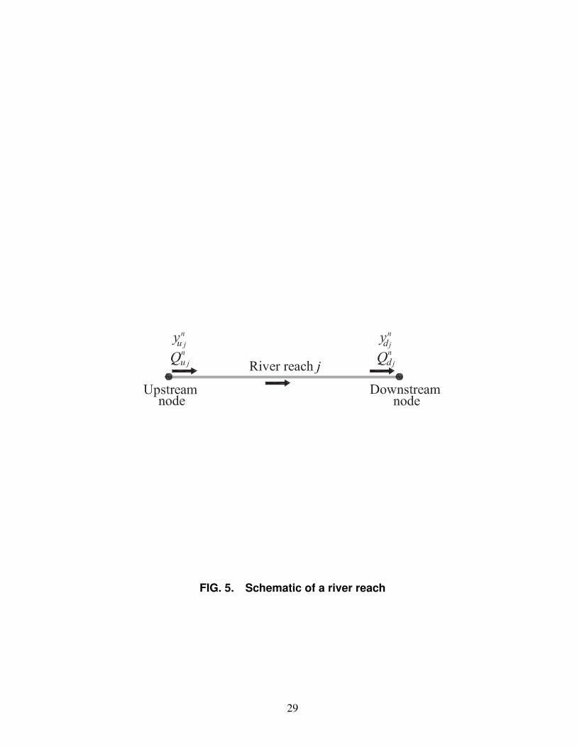
FIG. 5. Schematic of a river reach
29

FIG. 6. Schematic of a node
30
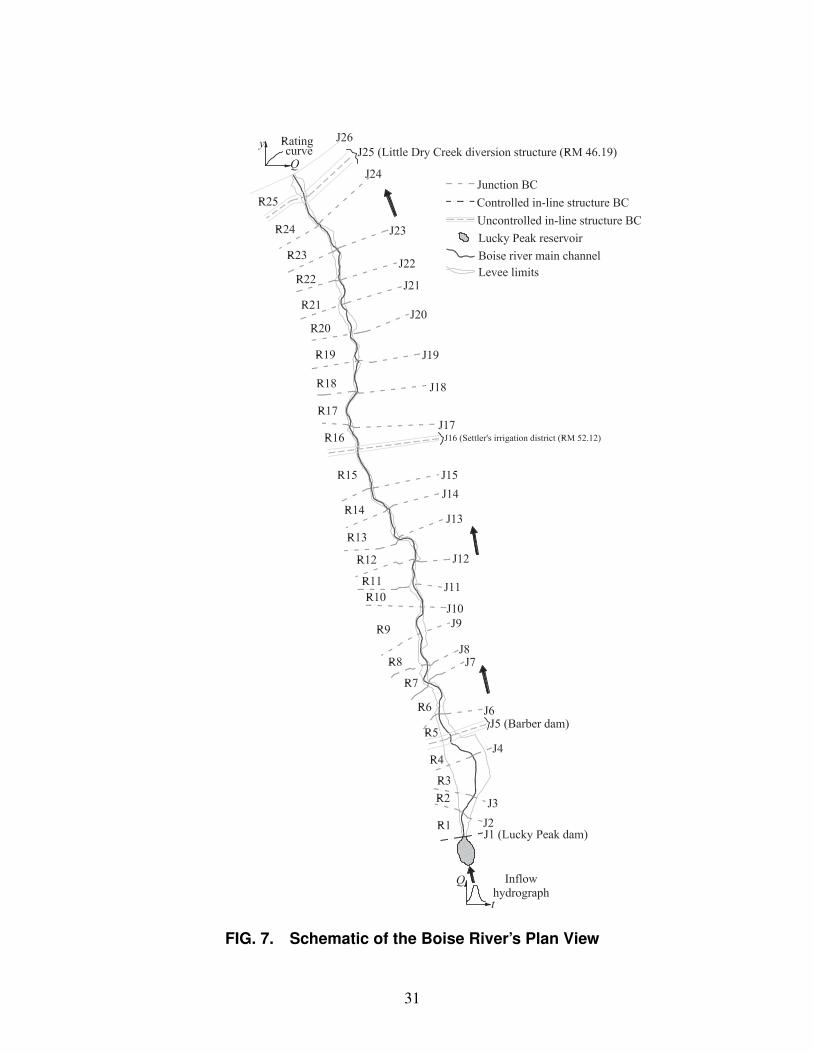
FIG. 7. Schematic of the Boise River’s Plan View
31
11/30/41 02/07/42 04/15/42 06/22/42 08/30/420
200
400
600
800
1,000
Date
Flo
w d
isch
arge
(m3 /s
)
FIG. 8. Inflow hydrograph (SWAT) at the Lucky Peak Reservoir in theBoise River Basin for the period between Nov 2041 and August 2042
32
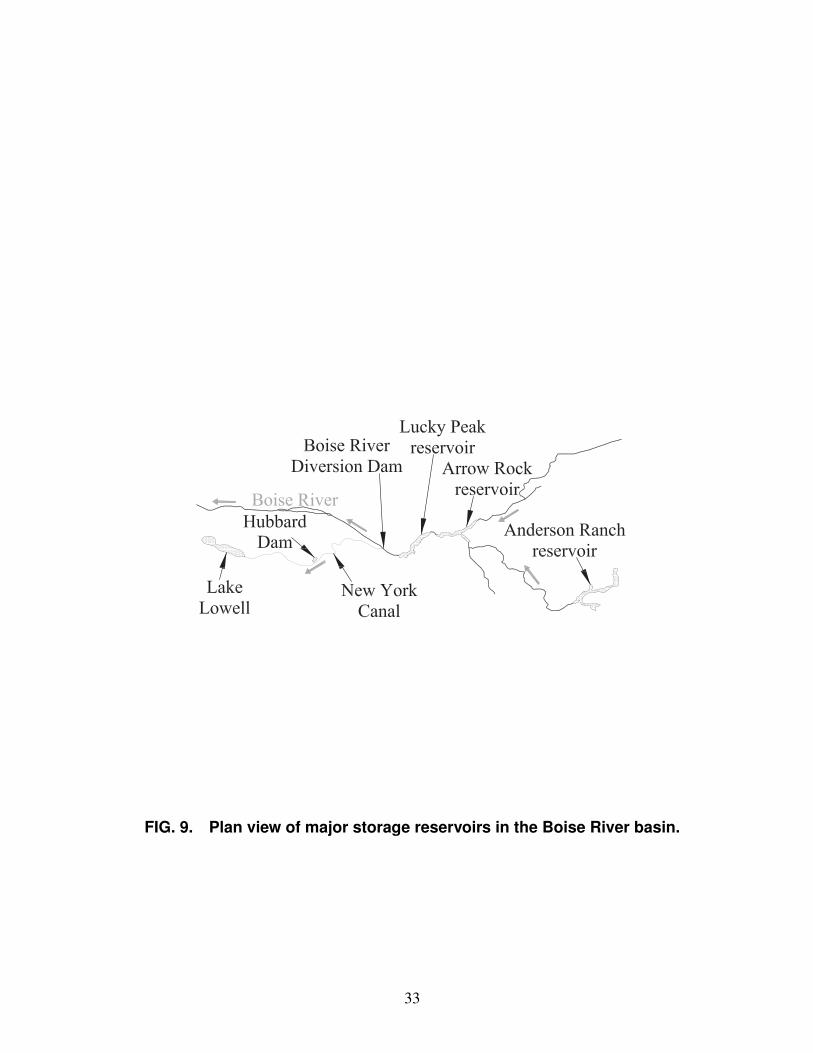
FIG. 9. Plan view of major storage reservoirs in the Boise River basin.
33
11/30/41 02/07/42 04/15/42 06/22/42 08/30/420
200
400
600
800
1,000
Date
Flo
w d
isch
arge
(m3 /s
)
FIG. 10. Inflow hydrograph subtracting active storage capacity of Ander-son Ranch, Arrow Rock, Hubbard reservoirs and Lake Lowell.
34
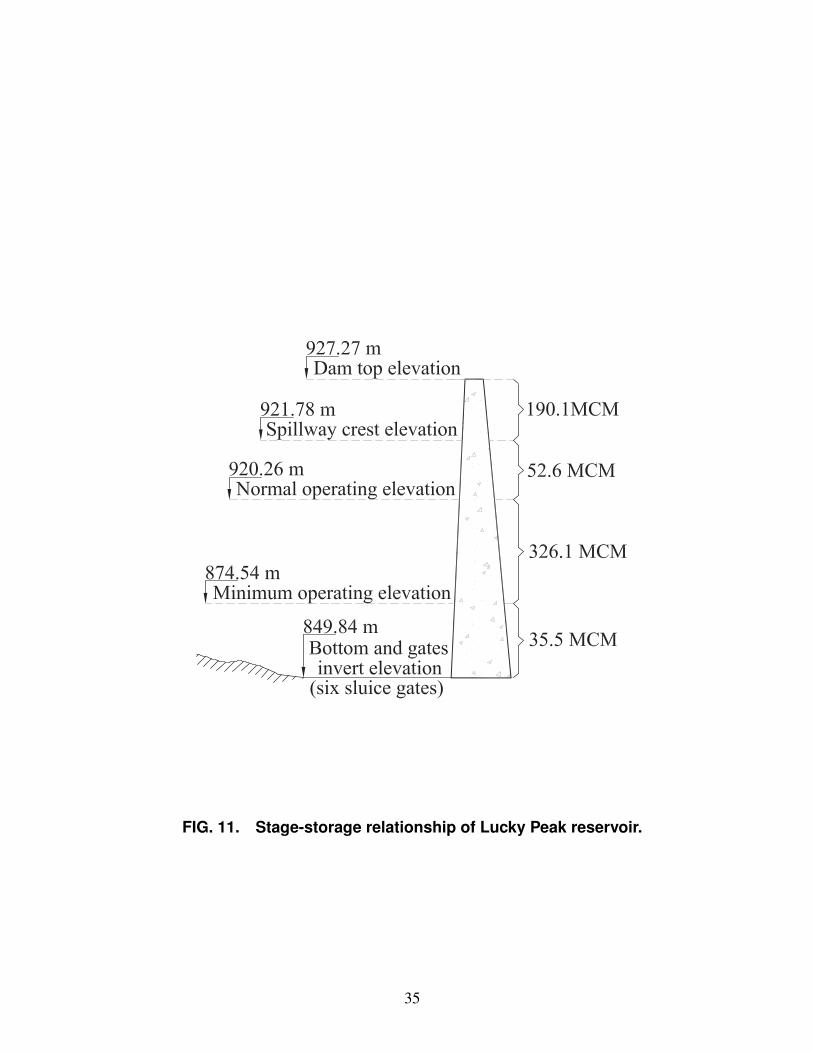
FIG. 11. Stage-storage relationship of Lucky Peak reservoir.
35
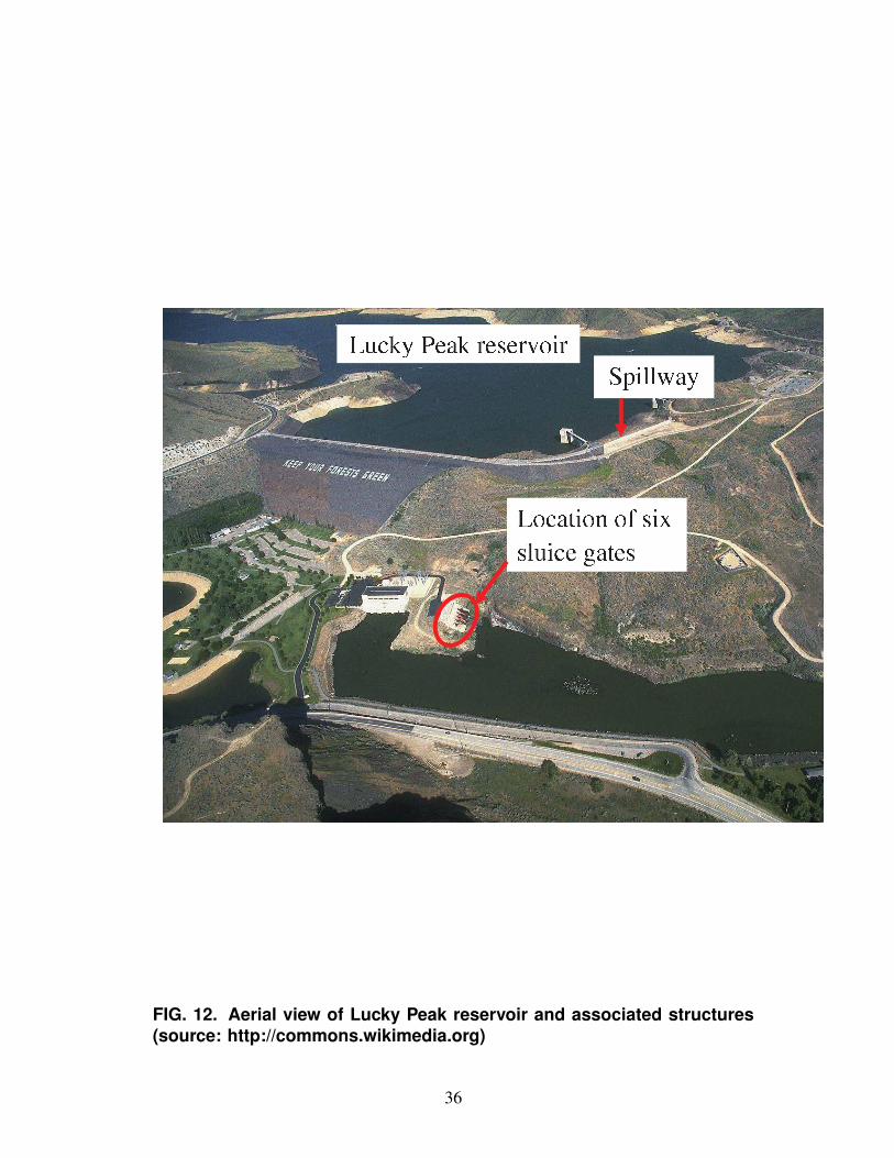
FIG. 12. Aerial view of Lucky Peak reservoir and associated structures(source: http://commons.wikimedia.org)
36
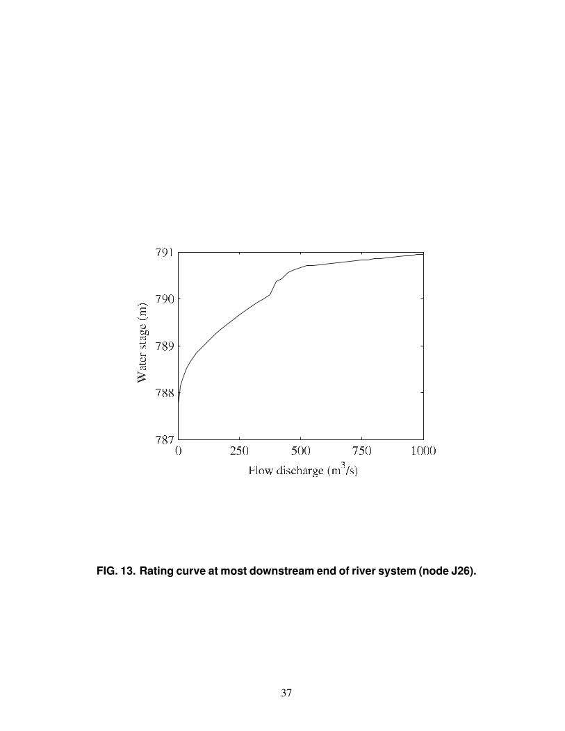
FIG. 13. Rating curve at most downstream end of river system (node J26).
37
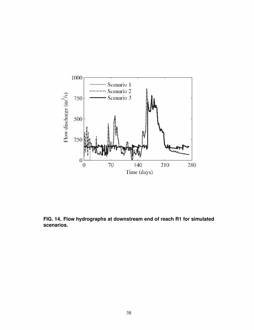
FIG. 14. Flow hydrographs at downstream end of reach R1 for simulatedscenarios.
38
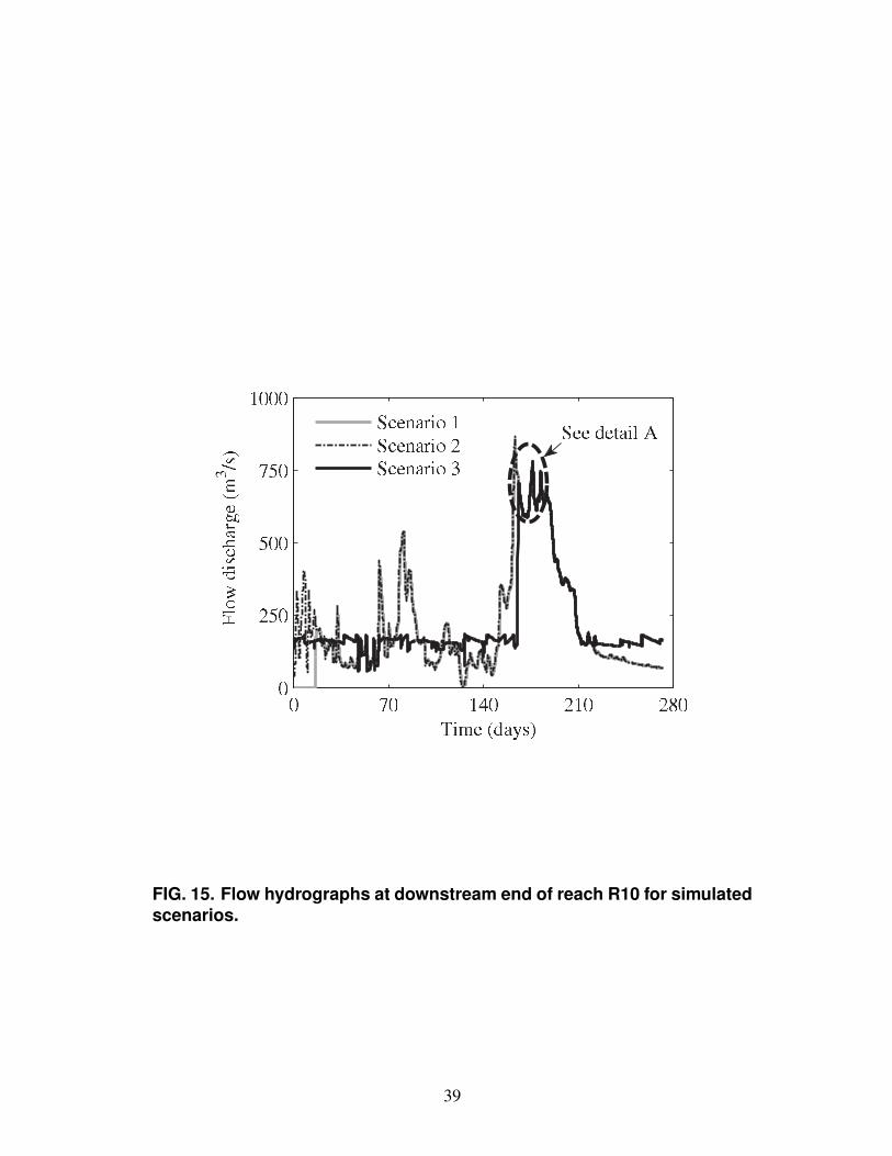
FIG. 15. Flow hydrographs at downstream end of reach R10 for simulatedscenarios.
39
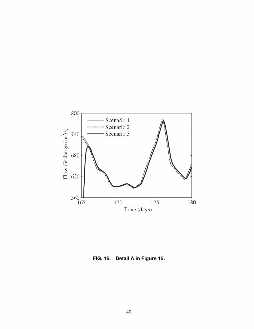
FIG. 16. Detail A in Figure 15.
40
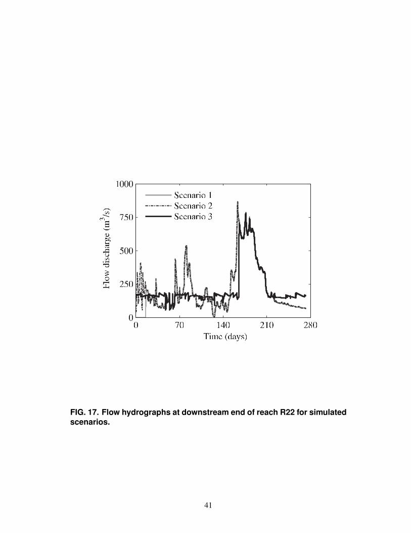
FIG. 17. Flow hydrographs at downstream end of reach R22 for simulatedscenarios.
41
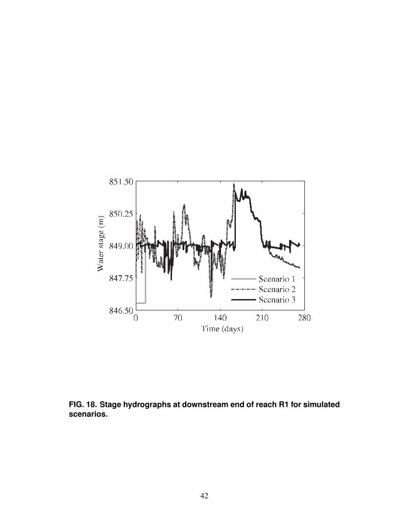
FIG. 18. Stage hydrographs at downstream end of reach R1 for simulatedscenarios.
42
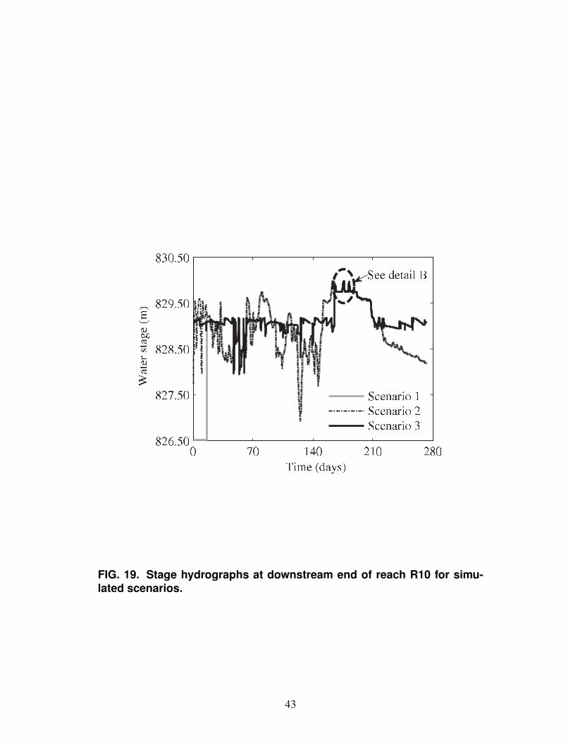
FIG. 19. Stage hydrographs at downstream end of reach R10 for simu-lated scenarios.
43
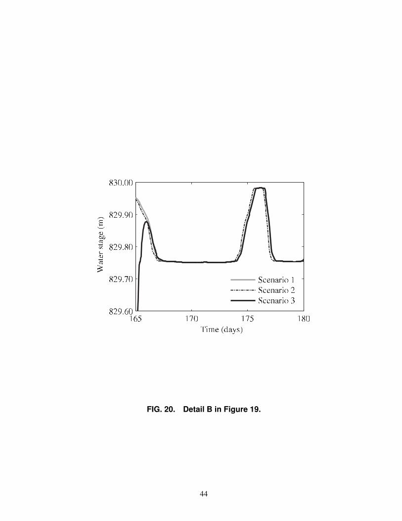
FIG. 20. Detail B in Figure 19.
44
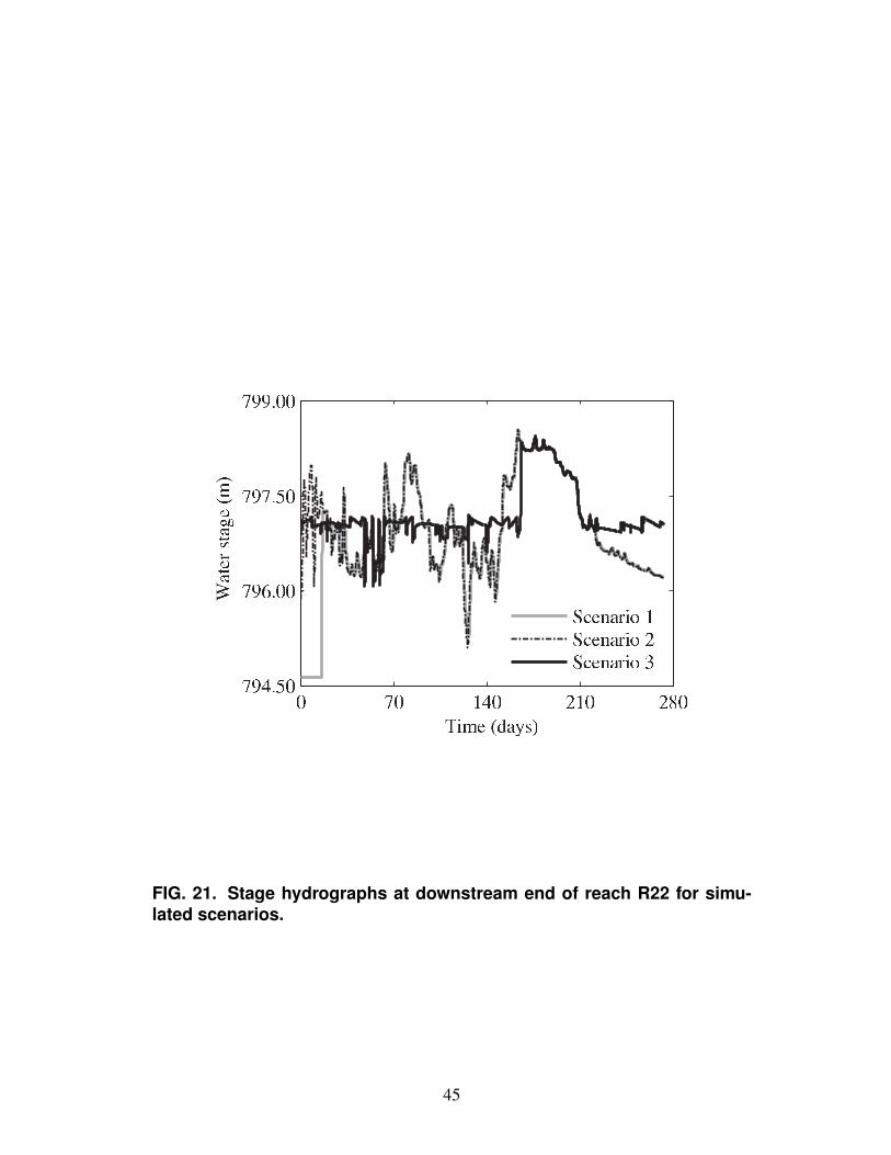
FIG. 21. Stage hydrographs at downstream end of reach R22 for simu-lated scenarios.
45
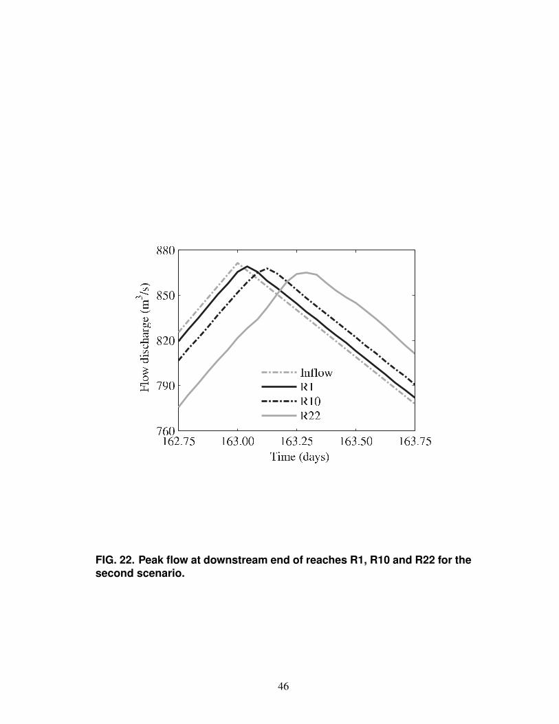
FIG. 22. Peak flow at downstream end of reaches R1, R10 and R22 for thesecond scenario.
46
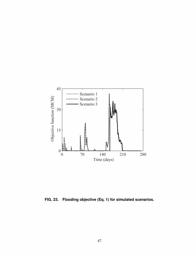
0 70 140 210 2800
15
30
45
Time (days)
Obj
ectiv
e fu
nctio
n (M
CM
) Scenario 1Scenario 2Scenario 3
FIG. 23. Flooding objective (Eq. 1) for simulated scenarios.
47
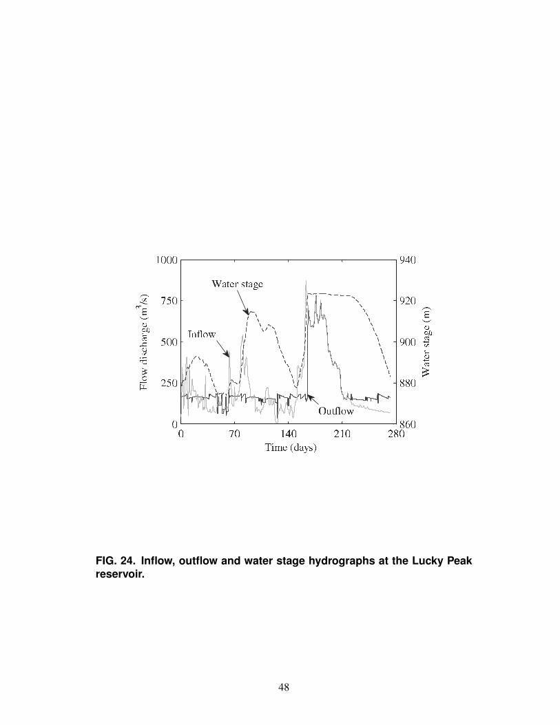
FIG. 24. Inflow, outflow and water stage hydrographs at the Lucky Peakreservoir.
48
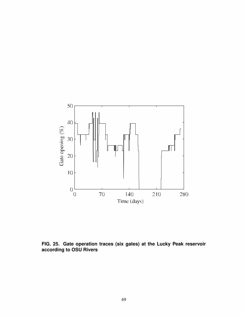
FIG. 25. Gate operation traces (six gates) at the Lucky Peak reservoiraccording to OSU Rivers
49
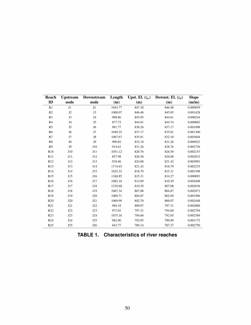
Reach Upstream Downstream Length Upst. El. (zu) Downst. El. (zd) SlopeID node node (m) (m) (m) (m/m)R1 J1 J2 1043.77 847.38 846.48 0.000859R2 J2 J3 1000.07 846.48 845.05 0.001428R3 J3 J4 998.86 845.05 844.81 0.000244R4 J4 J5 877.72 844.81 844.74 0.000082R5 J5 J6 991.77 838.26 837.17 0.001098R6 J6 J7 1049.35 837.17 835.81 0.001300R7 J7 J8 1007.67 835.81 832.18 0.003604R8 J8 J9 990.85 832.18 831.26 0.000922R9 J9 J10 914.63 831.26 828.76 0.002736
R10 J10 J11 1051.12 828.76 826.50 0.002153R11 J11 J12 857.98 826.50 824.08 0.002815R12 J12 J13 918.46 824.08 821.42 0.002901R13 J13 J14 1174.63 821.42 818.79 0.002235R14 J14 J15 1025.32 818.79 815.31 0.003398R15 J15 J16 1160.85 815.31 814.27 0.000893R16 J16 J17 1082.18 812.89 810.29 0.002408R17 J17 J18 1218.60 810.29 807.08 0.002636R18 J18 J19 1067.34 807.08 804.87 0.002071R19 J19 J20 1089.71 804.87 802.69 0.001996R20 J20 J21 1069.99 802.70 800.07 0.002448R21 J21 J22 984.18 800.07 797.31 0.002806R22 J22 J23 971.03 797.31 794.60 0.002794R23 J23 J24 1075.16 794.60 792.05 0.002369R24 J24 J25 982.00 792.05 790.90 0.001172R25 J25 J26 643.77 789.14 787.37 0.002750
TABLE 1. Characteristics of river reaches
50