To appear in the Journal of Computerized Medical Imaging and Graphics, 1994.

A Dynamic Finite Element Surface Model

for Segmentation and Tracking in

Multidimensional Medical Images with

Application to Cardiac 4D Image Analysis

Tim McInerney and Demetri Terzopoulos

Department of Computer Science, University of Toronto, Toronto, ON, Canada M5S 1A4

Abstract

This paper presents a physics-based approach to anatomical surface segmentation,reconstruction, and tracking in multidimensional medical images. The approach makesuse of a dynamic \balloon" model|a spherical thin-plate under tension surface splinewhich deforms elastically to �t the image data. The �tting process is mediated byinternal forces stemming from the elastic properties of the spline and external forceswhich are produced from the data. The forces interact in accordance with Lagrangianequations of motion that adjust the model's deformational degrees of freedom to �tthe data. We employ the �nite element method to represent the continuous surfacein the form of weighted sums of local polynomial basis functions. We use a quintictriangular �nite element whose nodal variables include positions as well as the �rstand second partial derivatives of the surface. We describe a system, implemented ona high performance graphics workstation, which applies the model �tting technique tothe segmentation of the cardiac LV surface in volume (3D) CT images and LV trackingin dynamic volume (4D) CT images to estimate its nonrigid motion over the cardiaccycle. The system features a graphical user interface which minimizes error by a�ord-ing specialist users interactive control over the dynamic model �tting process.

Keywords: 3D/4D Medical Image Analysis, Deformable Models, Finite Elements,Dynamics, Cardiac LV Segmentation, Nonrigid Motion Tracking, Visualization, Inter-action.

1 Introduction

CT, MRI, PET and other noninvasive medical imaging technologies can provide exceptionalviews of internal anatomical structures, but the computer aided visualization, manipula-tion, and quantitative analysis of the multidimensional image data they produce is still

1

limited. State-of-the-art medical imagers generate massive databases of static volume (3D)and dynamic volume (4D) images. These data sets, which usually su�er from samplingartifacts, spatial aliasing, and noise, are essentially \blocks of granite" with meaningful em-bedded structures. An important problem is to extract the surface elements belonging to ananatomical structure (the segmentation step) and to integrate these surface elements intoa globally coherent surface model of the structure (the reconstruction step). Certain diag-nostic procedures also require the tracking and deformation analysis of nonrigidly movinganatomical surfaces; e.g., the stretching of the left ventricle (LV) during the cardiac cycleis directly related to heart condition. The ease and accuracy of such procedures can becritically dependent upon the model used. Dynamic models are needed which are robustagainst noise-corrupted data and which are capable of accurately representing the complexgeometries of anatomical surfaces while permitting the quantitative measurement of highlynonrigid tissue kinematics.

This paper describes a physics-based modeling approach that addresses the surface seg-mentation and reconstruction problems, as well as the geometric analysis and nonrigid mo-tion estimation problems. We develop a dynamic, elastically deformable surface model whosedeformation is governed by basic laws of nonrigid motion. The formulation of the motionequations includes a strain energy, simulated forces, and other physical quantities. The sur-face strain energy stems from a thin-plate under tension variational spline. Deformationresults from the action of internal spline forces which impose surface continuity constraintsand external forces which �t the surface to the image data. The inherently dynamic formu-lation of the model makes it suitable both for static anatomical surface reconstruction andfor problems involving the reconstruction and tracking of nonrigidly moving organs.

To deal with closed anatomical surfaces, we formulate a deformable \balloon" model thatis topologically isomorphic to a sphere. We employ the �nite element method to spatiallydiscretize the balloon, uniformly tessellating it into a set of connected triangular elementdomains. The �nite element method provides an analytic, piecewise polynomial surfacerepresentation that is (C1) continuous across triangles. We use a quintic �nite element whosenodal variables include not only the nodal positions, but also the �rst and second parametricpartial derivatives of the surface. The element is naturally suited to the surface energyfunctional because these same partial derivatives occur in the thin-plate under tension energyexpression. The existence of parametric derivative nodal variables facilitates the computationof the di�erential properties of the modeled surface. In particular, the nodal variables andtheir time derivatives can be useful for computing the surface curvature, enclosed volume,and motion properties of anatomical surfaces.

We have implemented a system on a high performance graphics workstation which appliesthe dynamic model �tting technique to the segmentation of the LV surface in cardiac volume(3D) CT images and LV tracking in dynamic volume (4D) CT images in order to estimatenonrigid LV motion over the cardiac cycle. The system includes a graphical user interfacewhich provides interactive visualization and a�ords control over the model �tting process.The interface allows a user to select the initial size and location of the model and to exertinteractive forces on the model as it deforms to �t the data. This type of interactive control isdesirable in medical image analysis applications where there is low tolerance for inaccuracy,because it allows specialist users to exploit their knowledge to correct model �tting errors.

2

2 Background

The literature on segmentation and surface reconstruction in 3D medical images includesboth manual and automatic techniques. The dominant manual method is slice-editing. Inmanual slice-editing a skilled operator, using a computer mouse, pen, or trackball traces theregion of interest on each slice of the volume. This labor intensive method su�ers from manydrawbacks, such as di�culties in achieving reproducible segmentation results, di�culties incomparing measurements from di�erent operators, and di�culties deducing 3D structurefrom 2D slices. The technique can be speeded up and made more reproducible, however,through the use of contour extraction methods such as interactive snakes [1, 2].

The traditional automatic segmentation methods, such as density thresholding and theapplication of (2D or 3D) edge operators, have many well-known problems. Edge detectionand the more recent marching cube [3] technique reduce volume data into something thatis more readily displayed through 3D graphics, such as surface elements. However, theyemploy only the local properties of the image data; hence, they raise the di�cult problem ofestablishing the connectivity of surface trace elements in order to assemble sensible globalsurface structures [4]. These di�culties have prompted some researchers to settle for merelyvisualizing the volume data in its original form using morphology [5] or volume renderingtechniques [6]. Unlike global surface models, however, these voxel-display representations donot attempt to capture the geometric structure of anatomical structures; hence, they do nottreat the data in a manner consistent with the physical properties of the imaged objects.

Deformable surface models are a promising approach to extracting anatomically mean-ingful structures from volume data. The dynamic form of the deformable model �ttingtechnique described in this paper was �rst introduced by Terzopoulos, Witkin, and Kass [7].They proposed a dynamic deformable cylinder model constructed from generalized splines,along with force �eld techniques to �t the model to image data. This dynamic approach isbeing pursued by several researchers in computational vision [8, 9, 10, 11, 12, 13, 14]. Theuse of �nite element representations for variational problems in vision were �rst exploredin [15]. Our formulation applies the �nite element method to the thin-plate under tensionspline proposed in [16] in order to derive discrete nonrigid dynamics equations. The �niteelement representation yields piecewise continuous deformable surface models that generallyrequire fewer variables for similar accuracy compared to �nite di�erence approaches.

Our work is related to that of Young [17][18] and Cohen and Cohen [19, 20] who alsodevelop 3D deformable surface models which are based on the thin-plate under tension spline.Young �ts an open bicubic Hermitian �nite element based surface to the 3D locations of thecoronary arteries at diastasis. The parameters of the time{varying displacement �eld werethen �tted to the tracked displacements of the bifurcation points of the coronary arteries.Cohen and Cohen �t a cylindrical, bicubic Hermitian �nite element based surface to MRIimages of the LV. Another relevant deformable model is the discrete model developed byMiller et al. [21], which is subdivided and �tted to CT volume images by a relaxationprocess that minimizes a set of constraints such as the distance to the data or the localcurvature of the model.

In our work we develop a closed 3D surface model based on a quintic triangular �niteelement with position and derivative nodal variables. The model begins as a uniformly tessel-lated icosahedron which may subdivide repeatedly to attain the desired geometric resolution.Our model is dynamic in the sense that it undergoes deformations that are governed by non-

3

(a) (b) (c)

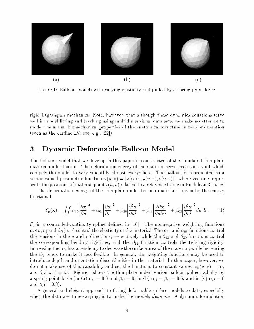
Figure 1: Balloon models with varying elasticity and pulled by a spring point force.

rigid Lagrangian mechanics. Note, however, that although these dynamics equations servewell in model �tting and tracking using multidimensional data sets, we make no attempt tomodel the actual biomechanical properties of the anatomical structure under consideration(such as the cardiac LV; see, e.g., [22]).

3 Dynamic Deformable Balloon Model

The balloon model that we develop in this paper is constructed of the simulated thin-platematerial under tension. The deformation energy of the material serves as a constraint whichcompels the model to vary smoothly almost everywhere. The balloon is represented as avector-valued parametric function x(u; v) = [x(u; v); y(u; v); z(u; v)]> where vector x repre-sents the positions of material points (u; v) relative to a reference frame in Euclidean 3-space.

The deformation energy of the thin-plate under tension material is given by the energyfunctional

Ep(x) =Z Z

�10

�����@x@u�����2

+ �01

�����@x@v�����2

+ �20

�����@2x

@u2

�����2

+ �11

����� @2x

@u@v

�����2

+ �02

�����@2x

@v2

�����2

du dv: (1)

Ep is a controlled-continuity spline de�ned in [16]. The nonnegative weighting functions�ij(u; v) and �ij(u; v) control the elasticity of the material. The �10 and �01 functions controlthe tensions in the u and v directions, respectively, while the �02 and �20 functions controlthe corresponding bending rigidities, and the �11 function controls the twisting rigidity.Increasing the �ij has a tendency to decrease the surface area of the material, while increasingthe �ij tends to make it less exible. In general, the weighting functions may be used tointroduce depth and orientation discontinuities in the material. In this paper, however, wedo not make use of this capability and set the functions to constant values �ij(u; v) = �ij

and �ij(u; v) = �ij. Figure 1 shows the thin plate under tension balloon pulled radially bya spring point force (in (a) �ij = 0:8 and �ij = 0, in (b) �ij = �ij = 0:5, and in (c) �ij = 0and �ij = 0:8):

A general and elegant approach to �tting deformable surface models to data, especiallywhen the data are time-varying, is to make the models dynamic. A dynamic formulation

4

imposes a natural temporal continuity on the model, thereby permitting a smoothly animateddisplay of the data �tting process. It also allows a user to interact with the model by applyingconstraint forces to pull it out of local minima towards the correct solution.

In a Lagrangian dynamics formulation, the positions of material points becomes a time-dependent function x(u; v; t) and we imbue the simulated material with mass and dampingdensities. The deformation energy yields internal elastic forces, and Ep(x) is minimizedwhen these forces equilibrate against externally applied forces and the model stabilizes:@x=@t = @2x=@t2 = 0.

The dynamic behavior of the balloon model during the �tting process is governed by thesecond-order partial di�erential equations

�@2x

@t2+

@x

@t+ �xEp = f ; (2)

where the �rst term represents the inertial forces due to the mass density �(u; v), the secondterm represents the damping forces due to the damping density (u; v), the third termrepresents the elastic force which resist deformation, and �nally f(u; v; t) represents theexternal forces derived from the image data. The (generally nonlinear) data forces may beformalized as stemming from a data functional

Ed(x) = �Z Z

x>f du dv: (3)

4 Finite Element Representation

The �nite di�erence method or the �nite element method are applicable to computing nu-merical solutions to the function x(u; v; t). Finite di�erence solutions approximate the con-tinuous function x as a set of discrete nodes in space. A disadvantage of the �nite di�erenceapproach is that the continuity of the solution between nodes is not made explicit. The�nite element method, on the other hand, provides continuous surface approximations; thatis, the method approximates the unknown function x in terms of combinations of local basisfunctions [23].

To apply the �nite element method to our models, we tessellate the continuous materialdomain (u; v) into a mesh of M element subdomains Ej. We approximate x as a weightedsum of piecewise polynomial basis functions Ni:

x(u; v; t) � x̂(u; v; t) =nXi=1

Ni(u; v)qi(t); (4)

where qi is a vector of nodal variables associated with mesh node i.Substituting (4) into (2) yields the discrete equations of motion

M�q+C _q+Kq = fq; (5)

with q = [q>1 ; : : : ;q>

i ; : : : ;q>

n ]>, where the mass matrixM, damping matrix C, and sti�ness

matrix K are sparse, symmetric matrices and vector fq are nodal data forces. These global

matrices may be assembled from their associated local element matrices by expanding each

5

element matrix appropriately into a q � q matrix and then summing:

M =MXj=1

Mjq�q; C =

MXj=1

Cjq�q; K =

MXj=1

Kjq�q; fq =

MXj=1

f jq; (6)

where Mj , Cj , Kj, and f jq are element mass, damping, and sti�ness matrices, and nodaldata forces associated with element Ej; j = 1; : : : ;M .

We now derive expressions for Mj, Cj , Kj, and f jq from element kinetic and potentialenergy functionals. Let xj(u; v; t) be the position of material point (u; v) within Ej , and letqj denote the concatenation of nodal variables for all the nodes of Ej. Following (4), wewrite the element trial function

x̂j(u; v; t) =Nj(u; v)qj(t) � xj(u; v; t); (7)

where Nj are the element shape functions. Recall that the basis functions Ni are obtainedby superposing the shape functions associated with node i. The element velocity is @x̂j=@t =Nj _qj, where _qj(t) is the rate of change of the nodal variables.

The kinetic energy associated with element Ej is

1

2

Z ZEj

�@x̂j

>

@t

@x̂j

@tdu dv =

1

2_qj>

�Z ZEj

�Nj>Nj du dv�_qj =

1

2_qj>Mj _qj; (8)

where the element mass matrix is given by

Mj =Z ZEj

�Nj>Nj du dv: (9)

We introduce a simple velocity-proportional kinetic energy dissipation according to the(Raleigh) dissipation functional

1

2

Z ZEj

@x̂j>

@t

@x̂j

@tdu dv =

1

2_qj>Cj _qj: (10)

The element damping matrix is proportional to the mass matrix and is given by

Cj =Z ZEj

Nj>Nj du dv: (11)

According to (1) the element deformation matrix may be expressed as

Ejp(x) =Z ZEj

���j>

���j du dv; (12)

6

where the strain vector is

���j =

24@xj>

@u;@xj

>

@v;@2xj

>

@u2;@2xj

>

@u@v;@2xj

>

@v2

35>

= Lxj (13)

and the stress vector is

���j =

2664�j10I 0 0 0 00 �j

01I 0 0 00 0 �j

20I 0 00 0 0 �j

11I 00 0 0 0 �j

02I

3775 ���j = Dj���j ; (14)

with I a 3� 3 unit matrix. Using (7), we can write

���j = LNjqj = Bjqj; (15)

where Bj is the element strain matrix. Inserting the expressions for ���j and ���j into (12) yields

Ejp(x) = qj>

Kjqj; (16)

where the element sti�ness matrix is given by

Kj =Z ZEj

Bj>DjBj du dv: (17)

Finally, according to (3), the potential energy in element Ej due to data forces f j(u; v; t)is

�Z ZEj

x̂j>f j du dv = �qj>

Z ZEj

Nj>f j du dv = �qj>

f jq ; (18)

where the nodal data forces are given by

f jq =Z ZEj

Nj>f j du dv: (19)

5 Model Structure

The balloon model is a closed surface in Euclidean 3-space which is topologically isomorphicto a sphere. We initially discretize the balloon in the material coordinates (u; v) by tessellat-ing it into a set of 20 triangular elements to form an icosahedron. We chose the icosahedronbecause it has a simple representation in material coordinates and it has a regular structurein Euclidean 3-space, with each of its 12 nodes connected to �ve neighboring nodes.

The parametric equation which initially maps the material (ui; vi) coordinates of the 12icosahedron nodes into 3-space is given by

x(ui; vi) = a

0B@

cosui cos vicosui sin visinui

1CA ; (20)

7

where ��=2 � v � �=2 and �� � u < � and a � 0 is a radius parameter.

5.1 Triangular C1 Finite Element

(u ,v )3 3

(u ,v )2 2

(u ,v )1 1

ξ=0 1−ξ−η=0

(1,0)(0,0)

(0,1)

v

u

ξ

ηη

ξ

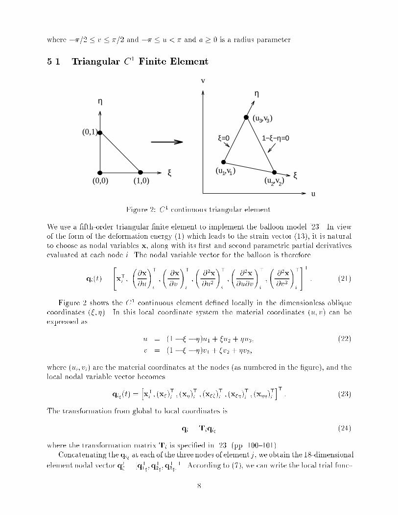
Figure 2: C1 continuous triangular element.

We use a �fth-order triangular �nite element to implement the balloon model [23]. In viewof the form of the deformation energy (1) which leads to the strain vector (13), it is naturalto choose as nodal variables x, along with its �rst and second parametric partial derivativesevaluated at each node i. The nodal variable vector for the balloon is therefore

qi(t) =

24x>i ;

@x

@u

!>

i

;

@x

@v

!>

i

;

@2x

@u2

!>

i

;

@2x

@u@v

!>

i

;

@2x

@v2

!>

i

35>

: (21)

Figure 2 shows the C1 continuous element de�ned locally in the dimensionless obliquecoordinates (�; �). In this local coordinate system the material coordinates (u; v) can beexpressed as

u = (1� � � �)u1 + �u2 + �u3; (22)

v = (1� � � �)v1 + �v2 + �v3;

where (ui; vi) are the material coordinates at the nodes (as numbered in the �gure), and thelocal nodal variable vector becomes

qi�(t) =hx>i ; (x�)

>

i; (x�)

>

i; (x��)

>

i; (x��)

>

i; (x��)

>

i

i>: (23)

The transformation from global to local coordinates is

qi = Tiqi� (24)

where the transformation matrix Ti is speci�ed in [23] (pp. 100{101).Concatenating the qi� at each of the three nodes of element j, we obtain the 18-dimensional

element nodal vector qj� = [q>1�;q>

2�;q>3�]

>. According to (7), we can write the local trial func-

8

tion asx̂j(�; �; t) = Nj(�; �)qj�(t): (25)

The nodal shape functions Ni(�; �) which are contained in the 18 � 18 matrix Nj are, fornode 1

N1 = �2(10�� 15�2 + 6�3 + 30��(� + �)); N2 = ��2(3� 2�� 3�2 + 6��)N3 = ��2(3 � 2�� 3�2 + 6��); N4 = 1

2�2�2(1� � + 2�)

N5 = ���2; N6 = 1

2�2�2(1 + 2� � �);

for node 2,

N7 = �2(10� � 15�2 + 6�3 + 15�2�); N8 = �2

2(�8� + 14�2 � 6�3 � 15�2�)

N9 = �2�

2(6� 4� � 3� � 3�2 + 3��); N10 = �2

4(2�(1� �)2 + 5�2�)

N11 = �2�

2(�2 + 2� + � + �2 � ��); N12 = �2�2�

4+ �3�2

2;

and for node 3,

N13 = �2(10� � 15�2 + 6�3 + 15�2�); N14 = ��2

2(6� 3� � 4� � 3�2 + 3��)

N15 = �2

2(�8� + 14�2 � 6�3 � 15�2�); N16 = �2�2�

4+ �2�3

2

N17 = ��2

2(�2 + � + 2� + �2 � ��); N18 = �

2

4(2�(1 � �)2 + 5�2�);

where � = 1� � � �.Note that the polynomial basis of the element is complete up to fourth-order terms and

contains three �fth-order terms [23]. The trial functions are C1 within elements and theyensure C1 continuity between elements. Since (1) contains up to second order derivatives,the element is conforming.

The shape functions are expressed in terms of the local coordinates (�; �) and it is conve-nient to work with these coordinates. Thus, the required derivatives of the shape functionsin the strain matrix B are computed using repeated applications of the chain rule and equa-tion (23). Also, a function f(u; v) may be integrated over Ej by transforming to the localcoordinate system as follows:

Z ZEj

f(u; v) du dv =Z ZEj

f(u(�; �); v(�; �)) detJ d� d�; (26)

where

J =

"@u@�

@v@�

@u

@�

@v

@�

#(27)

is the Jacobian matrix. These integrals are approximated using Gauss-Legendre quadraturerules [23].

5.2 Model Re�nement

Our implementation allows the balloon model to be re�ned during the �tting process bysubdividing the triangular elements. Each element spawns 4 child elements by connectingthe midpoints of its 3 edges (Fig. 3). This process may be applied recursively to each childelement. The connectivity of all new vertices formed in this fashion is six, while the original12 vertices of the icosahedron remain �ve-connected. Thus a low resolution model may be

9

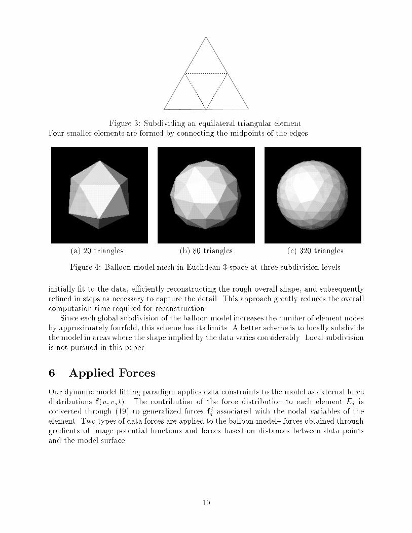
Figure 3: Subdividing an equilateral triangular element.Four smaller elements are formed by connecting the midpoints of the edges.

(a) 20 triangles (b) 80 triangles (c) 320 triangles

Figure 4: Balloon model mesh in Euclidean 3-space at three subdivision levels.

initially �t to the data, e�ciently reconstructing the rough overall shape, and subsequentlyre�ned in steps as necessary to capture the detail. This approach greatly reduces the overallcomputation time required for reconstruction.

Since each global subdivision of the balloon model increases the number of element nodesby approximately fourfold, this scheme has its limits. A better scheme is to locally subdividethe model in areas where the shape implied by the data varies considerably. Local subdivisionis not pursued in this paper.

6 Applied Forces

Our dynamic model �tting paradigm applies data constraints to the model as external forcedistributions f(u; v; t). The contribution of the force distribution to each element Ej isconverted through (19) to generalized forces f jq associated with the nodal variables of theelement. Two types of data forces are applied to the balloon model{ forces obtained throughgradients of image potential functions and forces based on distances between data pointsand the model surface.

10

6.1 3D Image Forces

When extracting and reconstructing surfaces from 3D image data, we design forces thatlocalize salient image features. For example, to attract our model towards signi�cant 3Dintensity edges (gradients) in some region of an image function I(x; y; z) we construct a 3Dpotential function

P (x; y; z) = �1 kr(G� � I)k+ �2 kOMD � Ik (28)

whose potential valleys (minima) coincide with the object surface [7]. In the �rst term on theright hand side of (28), G� denotes a 3D Gaussian smoothing �lter of characteristic width �.This �lter broadens or narrows the potential valleys of this term thus determining the extentof the region of attraction of the intensity gradient. Typically, the attraction has a relativelyshort range. In the second term, a 3D edge detector, the 3D Monga-Deriche (MD) operator[24], is applied to the image data to produce a 3D intensity edge �eld. The potential valleysof this term tend to be narrow and deep, complementing (and coinciding with) the widerbut more shallow valleys produced by the �rst term. A weighted combination of these termsis formed so the model will \slide down" the shallow valleys and then drop into the deepervalleys thus locking onto image edges.

The potential function produces a force distribution

f(x) = �rP (x)

krP (x)k(29)

on the model, where � controls the strength of the force. We normalize the image force as forbetter numerical stability [10]. Consequently, all signi�cant edge voxels, including spuriousedges, will attract the model equally. However, once the model converges towards the true3D edges of the object, the smoothing e�ect of the model will give it a tendency to ignorespurious 3D edges.

Note that to compute rP at any model point x(u; v) from a discrete 3D image data setI(i; j; k), we tri-linearly interpolate I(x) using values at the eight surrounding pixels.

6.2 Balloon In ation Force

When extracting object surfaces from 3D image data, the balloon model must �rst be ini-tialized within the object. If the model is not close enough to the surface of the object, theshort-range image forces de�ned previously may not attract it. For this reason, an internalpressure force is used to \in ate" the balloon model towards the object surface [7] [10]. Theforce takes the form

f = �1n(u; v); (30)

where n(u; v) is the unit normal vector to the model surface at the point x(u; v), and �1 isthe amplitude of this force. If �1 is negative, the force will de ate the balloon. We usuallyset the image force scale parameter � and �1 to be of the same order, with � slightly largerthan �1 so that a signi�cant 3D edge will stop the in ation, but with �1 large enough forthe model to pass through weak or spurious edges.

11

6.3 User and Constraint Forces

Accurate measurement of medical image structures is important in a clinical setting. For thisand other reasons, visualization and manual interaction are likely to remain essential in 3Dbiomedical image scenarios. Our dynamic modeling approach provides a facile interface tothe models through the use of force interaction tools. For example, as the model is deforming,the user may use the mouse to specify spring forces which pull the model towards signi�cantimage features, or to specify \pins" which constrain the model to interpolate �ducial featuresin the data that a specialist can identify.

Both the mouse and pin forces are implemented as long-range spring-like point forces

f(u; v) = � kp� x(up; vp)k (31)

proportional to the separation between the mouse or pin point p in space and the point ofin uence (up; vp) of the force on the model's surface.

We approximate (up; vp) as the model node with minimal distance to the point p, usinga heuristic local neighborhood search to �nd the nearest model node.

6.4 Parallel Numerical Integration

Our dynamic surface model is easiest to manipulate interactively during the �tting processif its motion is critically damped to minimize vibrations. Critical damping can be achievedby appropriately balancing the mass and damping distributions. Another way of eliminatingvibration while preserving useful dynamics is to set the mass density �(u; v) to zero, thusreducing (5) to

C _q+Kq = fq: (32)

This �rst-order dynamical system governs a model which has no inertia and comes to restas soon as all the forces equilibrate. Although (32) is simpler to implement and numericallymore e�cient, a model lacking inertia can experience di�culty tracking moving objects if ex-ternal forces are not persistently reliable due to weak, noisy, or missing data. Nonetheless, wehave successfully employed the �rst-order dynamic model (32) in our cardiac reconstructionand tracking system which is presented in the next section.

We integrate equation (32) forward through time using an explicit �rst-order Eulermethod. This method approximates the temporal derivatives with forward �nite di�er-ences. It updates the degrees of freedom q of the model from time t to time t+�t accordingto the formula

q(t+�t) = q(t) +�t(C(t))�1�f (t)q �Kq(t)

�: (33)

In our implementation, we do not explicitly assemble and factorize a global sti�nessmatrix K as is common practice in applied �nite element analysis. Instead, we update thenodal vectors q(t+�t)

i iteratively by computing the product Kjqj on an element-by-elementbasis using the element sti�ness matricesKj. This approach makes the model �tting processeasily parallelizable.

The deformable model is implemented as a list of �nite element data structures and a listof node data structures. The element structures contain pointers to their associated nodestructures. The following actions are repeated at each time step of the model �tting process:

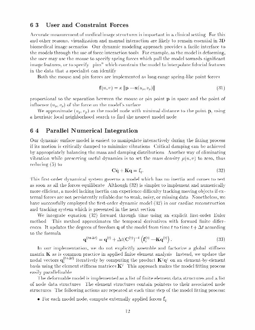
� For each model node, compute externally applied forces fq.

12

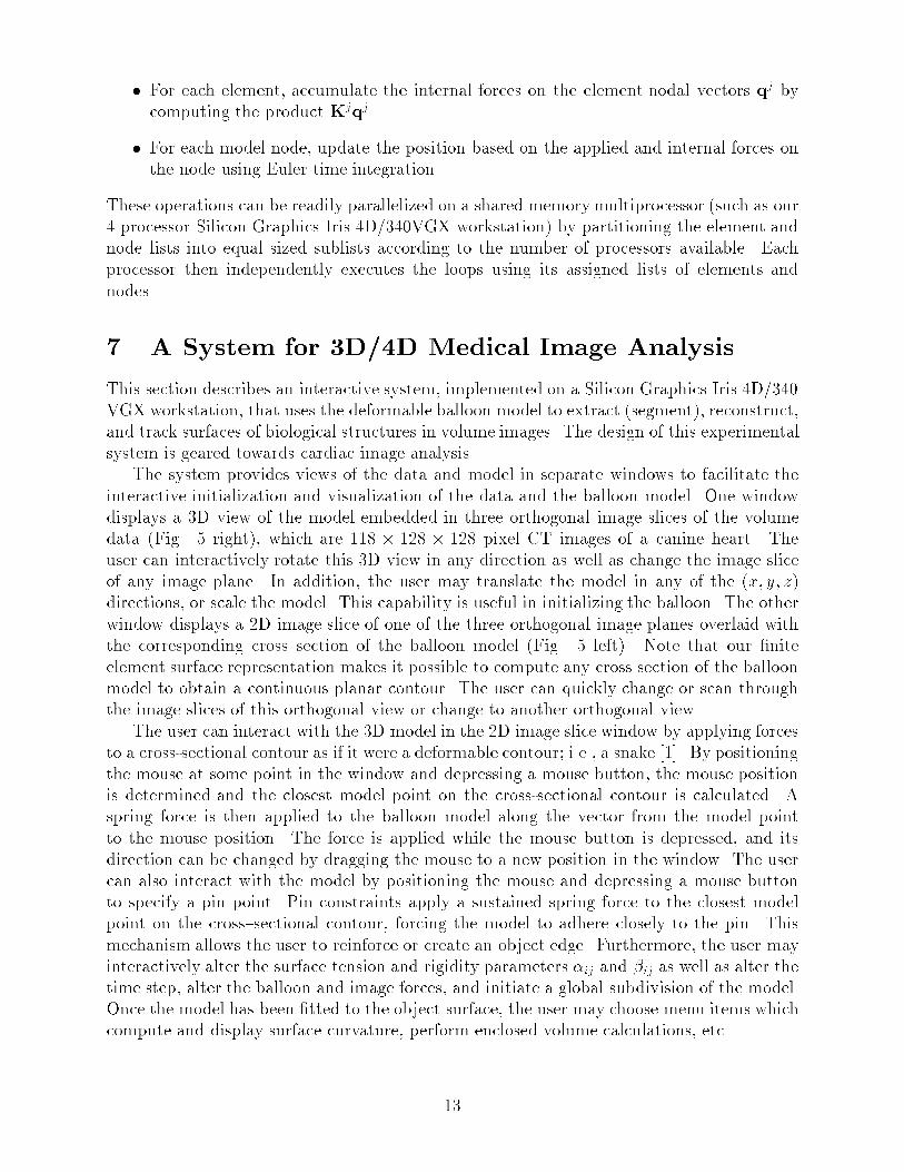
� For each element, accumulate the internal forces on the element nodal vectors qj bycomputing the product Kjqj.

� For each model node, update the position based on the applied and internal forces onthe node using Euler time integration.

These operations can be readily parallelized on a shared memorymultiprocessor (such as our4 processor Silicon Graphics Iris 4D/340VGX workstation) by partitioning the element andnode lists into equal sized sublists according to the number of processors available. Eachprocessor then independently executes the loops using its assigned lists of elements andnodes.

7 A System for 3D/4D Medical Image Analysis

This section describes an interactive system, implemented on a Silicon Graphics Iris 4D/340VGX workstation, that uses the deformable balloon model to extract (segment), reconstruct,and track surfaces of biological structures in volume images. The design of this experimentalsystem is geared towards cardiac image analysis.

The system provides views of the data and model in separate windows to facilitate theinteractive initialization and visualization of the data and the balloon model. One windowdisplays a 3D view of the model embedded in three orthogonal image slices of the volumedata (Fig. 5 right), which are 118 � 128 � 128 pixel CT images of a canine heart. Theuser can interactively rotate this 3D view in any direction as well as change the image sliceof any image plane. In addition, the user may translate the model in any of the (x; y; z)directions, or scale the model. This capability is useful in initializing the balloon. The otherwindow displays a 2D image slice of one of the three orthogonal image planes overlaid withthe corresponding cross section of the balloon model (Fig. 5 left). Note that our �niteelement surface representation makes it possible to compute any cross section of the balloonmodel to obtain a continuous planar contour. The user can quickly change or scan throughthe image slices of this orthogonal view or change to another orthogonal view.

The user can interact with the 3D model in the 2D image slice window by applying forcesto a cross-sectional contour as if it were a deformable contour; i.e., a snake [1]. By positioningthe mouse at some point in the window and depressing a mouse button, the mouse positionis determined and the closest model point on the cross-sectional contour is calculated. Aspring force is then applied to the balloon model along the vector from the model pointto the mouse position. The force is applied while the mouse button is depressed, and itsdirection can be changed by dragging the mouse to a new position in the window. The usercan also interact with the model by positioning the mouse and depressing a mouse buttonto specify a pin point. Pin constraints apply a sustained spring force to the closest modelpoint on the cross{sectional contour, forcing the model to adhere closely to the pin. Thismechanism allows the user to reinforce or create an object edge. Furthermore, the user mayinteractively alter the surface tension and rigidity parameters �ij and �ij as well as alter thetime step, alter the balloon and image forces, and initiate a global subdivision of the model.Once the model has been �tted to the object surface, the user may choose menu items whichcompute and display surface curvature, perform enclosed volume calculations, etc.

13

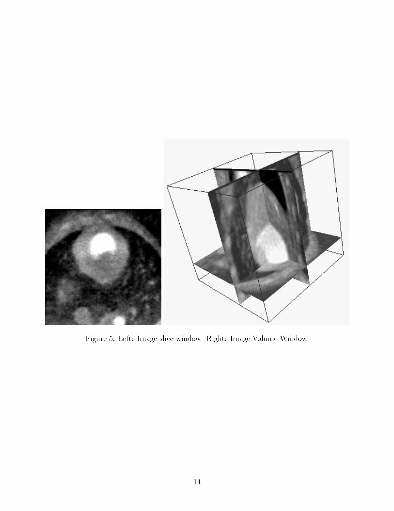
Figure 5: Left: Image slice window. Right: Image Volume Window.

14

(a) (b)

Figure 6: YZ and XY view edge detected image slices showing initial cross sections of theballoon model.The edge maps are generated by the application of the 3D Monga-Deriche (MD) operator.

7.1 The Segmentation/Reconstruction Process

To initiate the surface extraction/reconstruction process, the user scans through the imageslices in the 2D image window to locate the approximate center of the object to be extracted.This process is repeated for the two other orthogonal views. The user can observe the 3Dvolume view window during this procedure to aid in determining the object center. The userthen uses the mouse to specify the initial size and location of the model in the 2D imagewindow (Fig. 6). The initial model will then be constructed and will appear embedded inthe image slices in the 3D window. The user can further adjust the size and location of themodel in either of the windows.

The user may specify an initial model resolution level. Typically we begin with a lowresolution model and then use the mouse to globally subdivide the model. It is also useful toinitially set the tension parameters �ij to be signi�cantly smaller than the rigidity parameters�ij. This allows an initially coarse balloon model to stretch more easily and quickly towardsthe edges of the heart. Once the model reaches the edges and the model has been subdivided,�ij is then increased to smooth the �ner resolution model.

Once the initial model has been speci�ed, the user may begin the model �tting (Fig.7). Before or during the model �tting procedure the user may specify any number of pinconstraints on the model. We determine by visual inspection when the �tting process iscompleted. The user can quickly scan the image slices in the 2D window to ascertain howwell the cross sections of the model �t the object edges. A possible automatic stoppingcriterion might monitor the average position change of the model nodes at each iteration toassess whether the model has achieved equilibrium.

7.2 Experiments

We used the interactive system to extract and reconstruct the left-ventricular chamber from3D CT images of a canine heart. The data set was acquired by the dynamic spatial re-

15

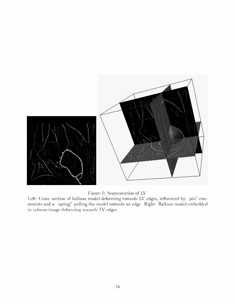
Figure 7: Segmentation of LV.Left: Cross{section of balloon model deforming towards LV edges, in uenced by \pin" con-straints and a \spring" pulling the model towards an edge. Right: Balloon model embeddedin volume image deforming towards LV edges.

16

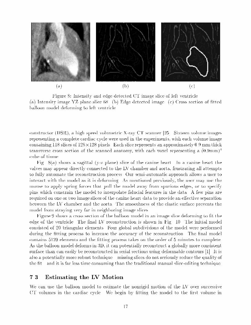
(a) (b) (c)

Figure 8: Intensity and edge detected CT image slice of left ventricle.(a) Intensity image YZ plane slice 68. (b) Edge detected image. (c) Cross section of �ttedballoon model deforming to left ventricle.

constructor (DSR), a high speed volumetric X-ray CT scanner [25]. Sixteen volume imagesrepresenting a complete cardiac cycle were used in the experiments, with each volume imagecontaining 118 slices of 128�128 pixels. Each slice represents an approximately 0.9 mm thicktransverse cross section of the scanned anatomy, with each voxel representing a (0:9mm)3

cube of tissue.Fig. 8(a) shows a sagittal (y-z plane) slice of the canine heart. In a canine heart the

valves may appear directly connected to the LV chamber and aorta, frustrating all attemptsto fully automate the reconstruction process. Our semi-automatic approach allows a user tointeract with the model as it is deforming. As mentioned previously, the user may use themouse to apply spring forces that pull the model away from spurious edges, or to specifypins which constrain the model to interpolate �ducial features in the data. A few pins arerequired on one or two image slices of the canine heart data to provide an e�ective separationbetween the LV chamber and the aorta. The smoothness of the elastic surface prevents themodel from straying very far in neighboring image slices.

Figure 9 shows a cross section of the balloon model in an image slice deforming to �t theedge of the ventricle. The �nal LV reconstruction is shown in Fig. 10. The initial modelconsisted of 20 triangular elements. Four global subdivisions of the model were performedduring the �tting process to increase the accuracy of the reconstruction. The �nal modelcontains 5120 elements and the �tting process takes on the order of 5 minutes to complete.As the balloon model deforms in 3D, it can potentially reconstruct a globally more consistentsurface than can easily be reconstructed in serial sections using deformable contours [1]. It isalso a potentially more robust technique|missing slices do not seriously reduce the quality ofthe �t|and it is far less time consuming than the traditional manual slice-editing technique.

7.3 Estimating the LV Motion

We can use the balloon model to estimate the nonrigid motion of the LV over successiveCT volumes in the cardiac cycle. We begin by �tting the model to the �rst volume in

17

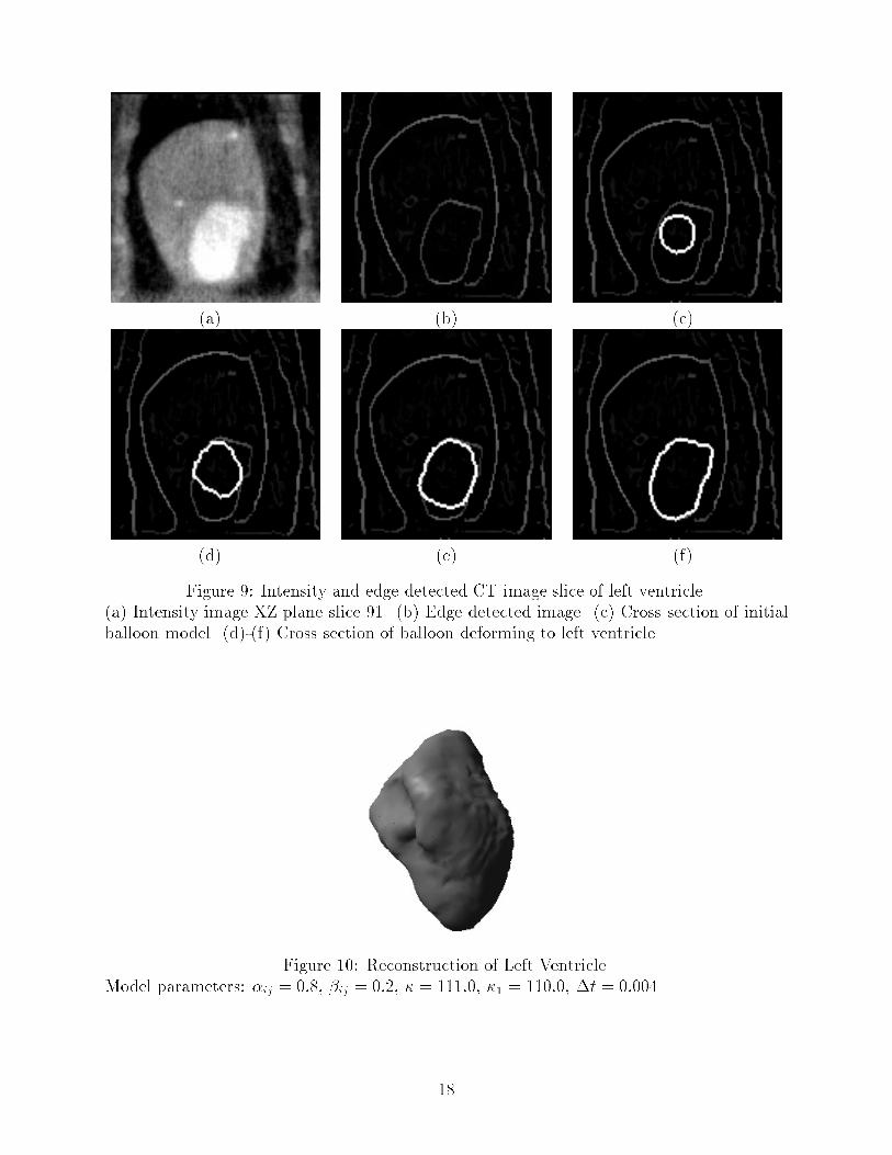
(a) (b) (c)

(d) (e) (f)

Figure 9: Intensity and edge detected CT image slice of left ventricle.(a) Intensity image XZ plane slice 91. (b) Edge detected image. (c) Cross section of initialballoon model. (d)-(f) Cross section of balloon deforming to left ventricle.

Figure 10: Reconstruction of Left Ventricle.Model parameters: �ij = 0:8, �ij = 0:2, � = 111:0, �1 = 110:0, �t = 0:004.

18

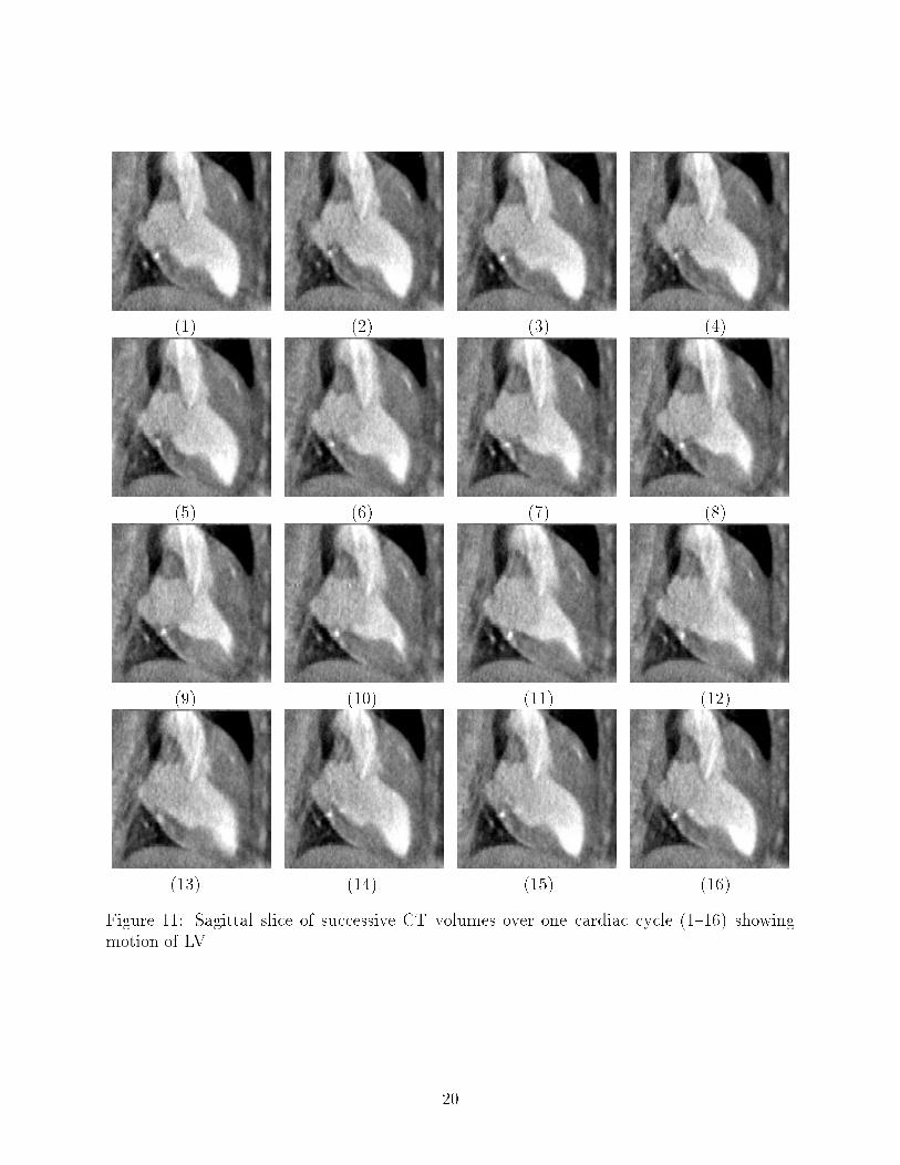
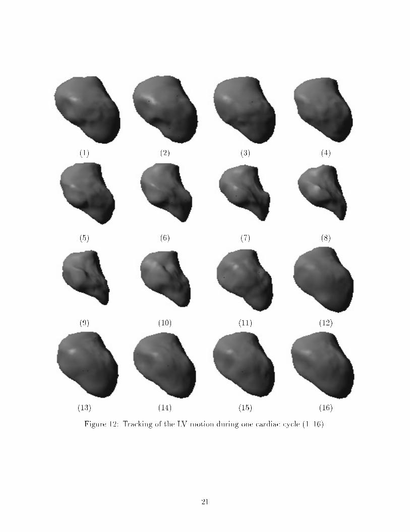
the sequence and use this �tted model as the starting point for the reconstruction of theLV in the next volume. We continue this process for all 16 volumes in the cardiac cycle.The tracking process allows the model to be \continuously" deformed by the time-varyingexternal data forces induced by the stream of volume images. The continuous �nite elementrepresentation enables us to track the approximate motion of any point of the LV surfacethrough the cardiac cycle (not just the nodal points).

Figure (11) shows sagittal slice 67 through the 16 successive CT volumes over one cardiaccycle. Figure (12) shows the reconstructed LV sequence. Each �tted model contains 1280elements and the entire �tting process, including the time required to input the 4D DSRdataset, takes only about 100 minutes to complete. This demonstrates the enormous poten-tial advantage of the dynamic deformable model approach compared with the time requiredto manually segment the LV. Once the initial 3D model has been �tted to the �rst volume,relatively small deformations are needed to �t subsequent volumes; consequently very littleuser intervention (i.e., application of pin constraints or spring forces) is necessary. Moreover,the �tting time per volume image should decrease as images are acquired at higher ratesbecause the interframe motion will be smaller. This should lead to proportionally greaterreductions in e�ort when the technique is applied to future image scanners capable of greatertemporal resolution.

8 Discussion

The 3D deformable model provides an e�cient, semi-automatic segmentation techniquewhich reconstructs a globally coherent surface between image slices that does not su�erfrom the banding artifacts often seen in surfaces reconstructed by independently contouringeach serial tomographic image. The surface model approximates the data across all the slices;hence, it is much less sensitive to noise than locally interpolatory segmentation schemes [3].

An extracted surface model with the aforementioned properties provides many optionsfor quantitative analysis of the anatomic object. In cardiology, for instance, volumetricparameters (end-diastolic and end-systolic volumes, stroke volume, and ejection ratio) arediagnostically signi�cant, while surface curvature extrema often have anatomical signi�cance.

We know from di�erential geometry that smooth 3D surfaces are uniquely characterized(up to rigid-body transformations) by their �rst and second fundamental forms [26]. Theparametric form of our surface model (i.e., x(u; v) = [x(u; v); y(u; v); z(u; v)]>) and, in partic-ular, the nodal variables (21) of its �nite element representation contain all the informationneeded to compute the �rst and second fundamental forms of the �tted model surface. Theintrinsic di�erential characteristics of the surface, such as the unit normal and the principalcurvatures, can be conveniently computed from this information, as can mean and Gaussiancurvatures. Furthermore, to compute the volume of the �tted balloon we can make use ofGauss's theorem which reduces a volume calculation problem to a surface integral of theform

=Z ZS

F (x) d�: (34)

The balloon model is composed of M surface elements de�ned parametrically within anelement in (25). Consequently, we can rewrite (34) as the sum of integrals over the surface

19

(1) (2) (3) (4)

(5) (6) (7) (8)

(9) (10) (11) (12)

(13) (14) (15) (16)

Figure 11: Sagittal slice of successive CT volumes over one cardiac cycle (1{16) showingmotion of LV.

20

(1) (2) (3) (4)

(5) (6) (7) (8)

(9) (10) (11) (12)

(13) (14) (15) (16)

Figure 12: Tracking of the LV motion during one cardiac cycle (1{16).

21

Figure 13: End-diastolic and end-systolic surfaces of LV during cardiac cycle.

elements as follows:

=MXi=1

Z ZSi

F (x) d� =Z ZSi

F (x(�; �)) detJ d� d�; (35)

where detJ = @x@�(�; �) � @x

@�(�; �)

is the Jacobian of transformation.By tracking a parametric surface over time, the dynamic deformable model technique

permits a direct analysis of the estimated nonrigid motion. For instance, the variation in theGaussian curvature of the �tted model over time can be used to estimate the local stretchingand shrinking of the LV surface during the cardiac cycle. It should be noted, however, thatfor the relatively smooth LV surface, the simple tracking scheme employed in this paperestimates the tangential component of the surface velocity �eld much less reliably than thenormal component. A more accurate estimation of the tangential component would requireadditional data or a priori information. For example, SPAMM images [27] depict transientmagnetic tags within the heart wall whose motion can be followed over several subsequentimages, providing both orthogonal components of the local velocity in the image plane [28].Our model can readily assimilate this type of information and that available from othersources. For instance,

� a priori information about nonrigidity could be included so that the model not onlydeforms to �t the data but also preserves some basic nonrigid constraints such asisometry or conformality [29].

� �ducial points can be extracted from the model surface and used as a guide when�tting the model to subsequent volumes in the sequence.

� the model can be generalized so that it subdivides elements in areas undergoing stretch-ing or bending or merge elements in areas that are less curved (cf. adaptive meshes

22

[29, 30, 31]). This would enable the elements to better follow the motion of the datapoints and allow for correspondence recovery.

Obviously, it is di�cult to assess the accuracy of our LV reconstruction and tracking re-sults from a single 4D dataset. A complete error analysis would also require quantitativecomparisons against images segmented manually by experts and is beyond the scope of thispaper.

9 Summary

We proposed a 3D elastically deformable balloon model for segmentation, reconstruction, andtracking of anatomical structures in multidimensional images. The surface of the model iscomposed of C1 triangular �nite elementswhose nodal variables include position and �rst andsecond parametric partial derivatives of the surface. Lagrangian equations of motion makethe dynamic model responsive to forces, derived from the 3D data, which deform its surface to�t the data in an elegant and intuitive manner. The �tting is carried out through numericaltime-integration of the motion equations. An iterative integration method is used thatexploits the parallelism of shared-memory multiprocessor architectures. This low-latencymethod supports real-time 3D display of the model as it extracts and tracks an anatomicalsurface. Furthermore, the model features a recursive, global subdivision capability whichcan �t a high resolution surface at low overall computational cost.

We described an experimental interactive system that demonstrates some of the capa-bilities of our model by applying it to 4D cardiac CT data. The system semi-automaticallysegments, reconstructs, and tracks the LV, allowing the user to initialize the model in theregion of interest, dynamically manipulate it during the data analysis, and alter the view-point, shading mode, and other visualization parameters at any time. The e�ective e�ciencygains that can accrue from a system of this sort should be even more dramatic with dynamicimaging at higher spatial and temporal resolution. Additional re�nements will increase themodel's potential to support reliable quantitative analysis of volume, form, and nonrigidmotion for diagnostic and other medical purposes. This is a promising direction for furtherwork.

Acknowledgements

DT is a Fellow of the Canadian Institute for Advanced Research. We thank the followingpeople for their cooperation: The cardiac CT images were made available by Eric Ho�manof the University of Pennsylvania Medical School and were redistributed to us courtesyof Dmitry Goldgof, University of South Florida. The Monga-Deriche edge detector wasprovided courtesy of Nicholas Ayache and Gregoire Malandain of INRIA, Paris, France.This research was supported by the Natural Sciences and Engineering Research Council ofCanada and the Information Technologies Research Center of Ontario.

References

[1] I. Carlbom, D. Terzopoulos, and K.M. Harris. Reconstructing and visualizing models of neu-

23

ronal dendrites. In N.M. Patrikalakis, editor, Scienti�c Visualization of Physical Phenomena,pages 623{638. Springer{Verlag, New York, 1991.

[2] A. Singh, L. von Kurowski, and M.-Y. Chiu. Cardiac MRI Segmentation Using DeformableModels. In Proc. IEEE Conf. on Computers and Cardiology, London, Sept. 1993.

[3] W.E. Lorenson and H.E. Cline. Marching Cubes, A High Resolution 3D Surface ConstructionAlgorithm. Computer Graphics, 21(4):163{169, 1987.

[4] P. Sander and S. Zucker. Inferring surface trace and di�erential structure from 3-D images.IEEE Trans. Pattern Analysis and Machine Intelligence, 12(9):833{854, 1990.

[5] S.R. Sternberg. Grayscale Morphology. Computer Vision, Graphics, and Image Processing,35:333{355, 1986.

[6] R.A. Drebin, L. Carpenter, and P. Hanrahan. Volume Rendering. Computer Graphics,22(4):65{74, 1988.

[7] D. Terzopoulos, A. Witkin, and M. Kass. Constraints on Deformable Models: Recovering 3DShape and Nonrigid motion. Arti�cial Intelligence, 36(1):91{123, 1988.

[8] D. Terzopoulos and D. Metaxas. Dynamic 3DModels with Local and Global Deformations: De-formable Superquadrics. IEEE Trans. Pattern Analysis and Machine Intelligence, 13(7):703{714, 1991.

[9] A. Pentland and B. Horowitz. Recovery of Nonrigid Motion and Structure. IEEE Trans.Pattern Analysis and Machine Intelligence, 13(7):730{742, July 1991.

[10] L.D. Cohen. On Active Contour Models and Balloons. In CVGIP: Image Understanding,volume 53(2), pages 211{218, March 1991.

[11] H. Delingette, M. Hebert, and K. Ikeuchi. Shape Representation and Image SegmentationUsing Deformable Surfaces. In Proc. IEEE Conf. Comp. Vision and Pattern Recognition,pages 467{472, June 1991.

[12] Y.F. Wang and J.F. Wang. Surface Reconstruction using Deformable Models with Interior andBoundary Constraints. IEEE Trans. Pattern Analysis and Machine Intelligence, 14(5):572{579, May 1992.

[13] T. McInerney. Finite Element Techniques for Fitting Deformable Models to 3D Data. Master'sthesis, Dept. of Computer Science, University of Toronto, Toronto, ON, Canada, 1992.

[14] D. Metaxas and D. Terzopoulos. Shape and nonrigid motion estimation through physics-basedsynthesis. IEEE Transactions on Pattern Analysis and Machine Intelligence, 15(6):580{591,1993.

[15] D. Terzopoulos. Multilevel computational processes for visual surface reconstruction. Com-puter Vision, Graphics, and Image Processing, 24:52{96, 1983.

[16] D. Terzopoulos. Regularization of Inverse Visual Problems Involving Discontinuities. IEEETrans. Pattern Analysis and Machine Intelligence, 8(4):413{424, 1986.

[17] A.A. Young. Epicardial Surface Estimation from Coronary Cineangiograms. Computer Vision,Graphics, and Image Processing, 47:11{127, 1989.

24

[18] A. Young. Epicardial deformation from coronary cineangiograms. In L. Glass, P. Hunter, andA. McCulloch, editors, in Theory of Heart, pages 175{207. Springer{Verlag, Heidelberg, 1991.

[19] I. Cohen, L.D. Cohen, and N. Ayache. Introducing New Deformable Surfaces to Segment 3DImages. In Proc. IEEE Conf. Comp. Vision and Pattern Recognition, pages 738{739, June1991.

[20] L.D. Cohen and I. Cohen. Deformable Models for 3D Medical Images Using Finite Elementsand Balloons. In Proc. IEEE Conf. Comp. Vision and Pattern Recognition, pages 592{598,June 1992.

[21] J.V. Miller, D.E. Breen, W.E. Lorensen, R.M. O'Bara, and M.J. Wozny. Geometrically De-formed Models. In Computer Graphics(SIGGRAPH'91), volume 25(4), pages 217{226, July1991.

[22] L. Glass, P. Hunter, and A. McCulloch, editors. Theory of Heart. Springer{Verlag, New York,1991.

[23] G. Dhatt and G. Touzot. The Finite Element Method Displayed. Wiley, New York, 1984.

[24] O. Monga and R. Deriche. 3D Edge Detection Using Recursive Filtering. In Proc. IEEE Conf.Comp. Vision and Pattern Recognition, June 1989.

[25] E.L. Ritman, R.A. Robb, and L.D. Harris. Imaging Physiological Functions: Experience withthe Dynamic Spatial Reconstruction. Praeger, New York, 1985.

[26] P. M. do Carmo. Di�erential Geometry of Curves and Surfaces. Prentice Hall, EnglewoodCli�s, New Jersey, 1976.

[27] L. Axel and L. Dougherty. Heart Wall Motion: Improved Method of Spatial Modulation ofMagnetization for MR Imaging. Radiology, 172:349{350, 1989.

[28] A. Young and L. Axel. Non-rigid Wall Motion Using MR Tagging. In Proc. IEEE Conf. Comp.Vision and Pattern Recognition, pages 399{404, June 1992.

[29] W.C. Huang and D.B. Goldgof. Left Ventricle Motion and Analysis by Adaptive-SizePhysically-based Models. In SPIE Proceedings, volume 1660{30, pages 299{310, Feb. 1992.

[30] W.-C. Huang and D. B. Goldgof. Adaptive-size meshes for rigid and nonrigid shape analysisand synthesis. IEEE Transactions on Pattern Analysis and Machine Intelligence, 15(6):611{616, 1993.

[31] M. Vasilescu and D. Terzopoulos. Adaptive meshes and shells: Irregular triangulation, discon-tinuities, and hierarchical subdivision. In IEEE Computer Society Conference on ComputerVision and Pattern Recognition (CVPR'92), pages 829{832, Champaign, IL, June 1992. IEEEComputer Society Press.

25