Embed Size (px)
Citation preview

A dynamic approach to short run economic fluctuations. The DAD/DAS
model.
Part 2.
The demand side of the model – the dynamic aggregate demand (DAD)
Macroeconomics II

Inflation and dynamics in the short run
• So far, to analyze the short run we have used – the IS-LM model (shows just the demand side) and
– Static AS/AD model
• Both theories are silent about – Inflation, and
– Dynamics
• Last week, we started to develop a dynamic aggregate demand and dynamic aggregate supply (DAD-DAS)
• The DAD-DAS model presents a dynamic short-run theory of output, inflation, and interest rates.

Introduction
• The dynamic model of aggregate demand and aggregate supply (DAD-DAS) determines both
– real GDP (Y), and
– the inflation rate (π)
• This theory is dynamic in the sense that the outcome in one period affects the outcome in the next period

• Instead of representing monetary policy by an exogenous money supply, the central bank will now be seen as following a monetary policy rule
– The central bank’s monetary policy rule adjusts interest rates automatically when output or inflation are not where they should be.
Introduction

Introduction
• The DAD-DAS model is built on the following concepts: – The Phillips Curve
– Adaptive expectations
• Which together built the supply side of the model - - we have done that last week – The IS curve (a negative relationship between the real
interest rate and aggregate demand)
– The Fisher effect
– The monetary policy rule of the central bank
• Which together built the demand side of the model (our job for today)
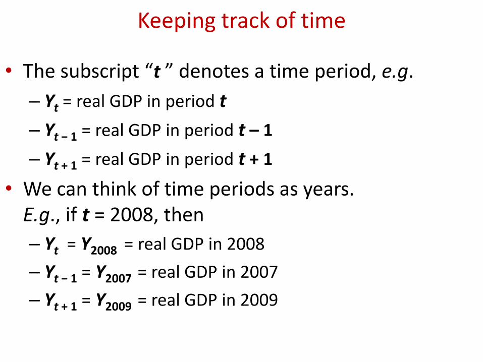
Keeping track of time
• The subscript “t ” denotes a time period, e.g.
– Yt = real GDP in period t
– Yt − 1 = real GDP in period t – 1
– Yt + 1 = real GDP in period t + 1
• We can think of time periods as years. E.g., if t = 2008, then
– Yt = Y2008 = real GDP in 2008
– Yt − 1 = Y2007 = real GDP in 2007
– Yt + 1 = Y2009 = real GDP in 2009

The model’s elements
• The DAD/DAS model has five equations and five endogenous variables:
– output, inflation, the real interest rate, the nominal interest rate, and expected inflation.
• We already know the supply side equation – the Phillips curve

Inflation: The Phillips Curve
tNttttuuE
)(
1
• Recall the Phillips Curve:
• Use the Okun’s Law to get the relationship bewteen inflation and output :
1 ( )t t t t t tE Y Y
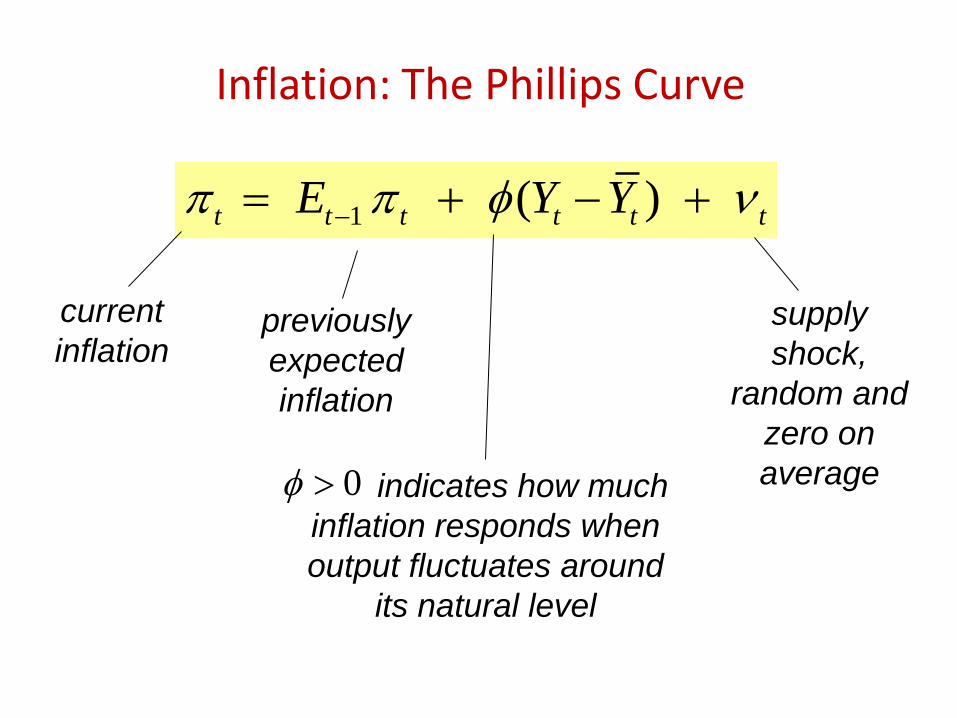
Inflation: The Phillips Curve
1 ( )t t t t t tE Y Y
previously
expected
inflation
current
inflation supply
shock,
random and
zero on
average indicates how much
inflation responds when
output fluctuates around
its natural level
0

Expected Inflation: Adaptive Expectations
1t t tE
Assumption: people expect
prices to continue rising at the
current inflation rate.
Examples: E2000π2001 = π2000; E2013π2014 = π2013; etc.

Phillips Curve
• At any particular time, inflation would be high if – people in the past were expecting it to be high
– current demand is high (relative to natural GDP)
– there is a high inflation shock. That is, if prices are rising rapidly for some exogenous reason such as scarcity of imported oil or drought-caused scarcity of food
tttttt YYE 1

Dynamic Aggregate Supply
ttt
tttttt
E
YYE
1
1Phillips Curve
Adaptive Expectations
ttttt YY 1DAS Curve
11 tttE
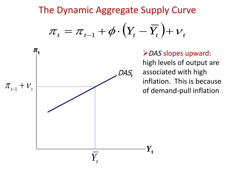
The Dynamic Aggregate Supply Curve
DAS slopes upward: high levels of output are associated with high inflation. This is because of demand-pull inflation
Yt
πt
DASt
tY
tt
1
ttttt YY 1

The Dynamic Aggregate Supply Curve
A change in previous period’s inflation shifts the DAS curve
Yt
π
DASt=2
tY
1t
ttttt
YY 1
0t
Assume
DASt=3
2t
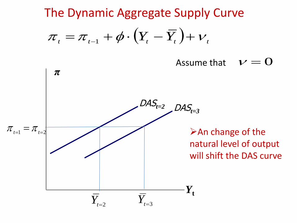
The Dynamic Aggregate Supply Curve
An change of the natural level of output will shift the DAS curve
Yt
π
DASt=2
2tY
21
tt
ttttt
YY 1
0
DASt=3
Assume that
3tY

The Dynamic Aggregate Supply Curve
A supply shock will shift the DAS curve
Yt
π
DASt=2
tY
1t
ttttt
YY 1
0312
tttand
DASt=3
32
tt
Assume that
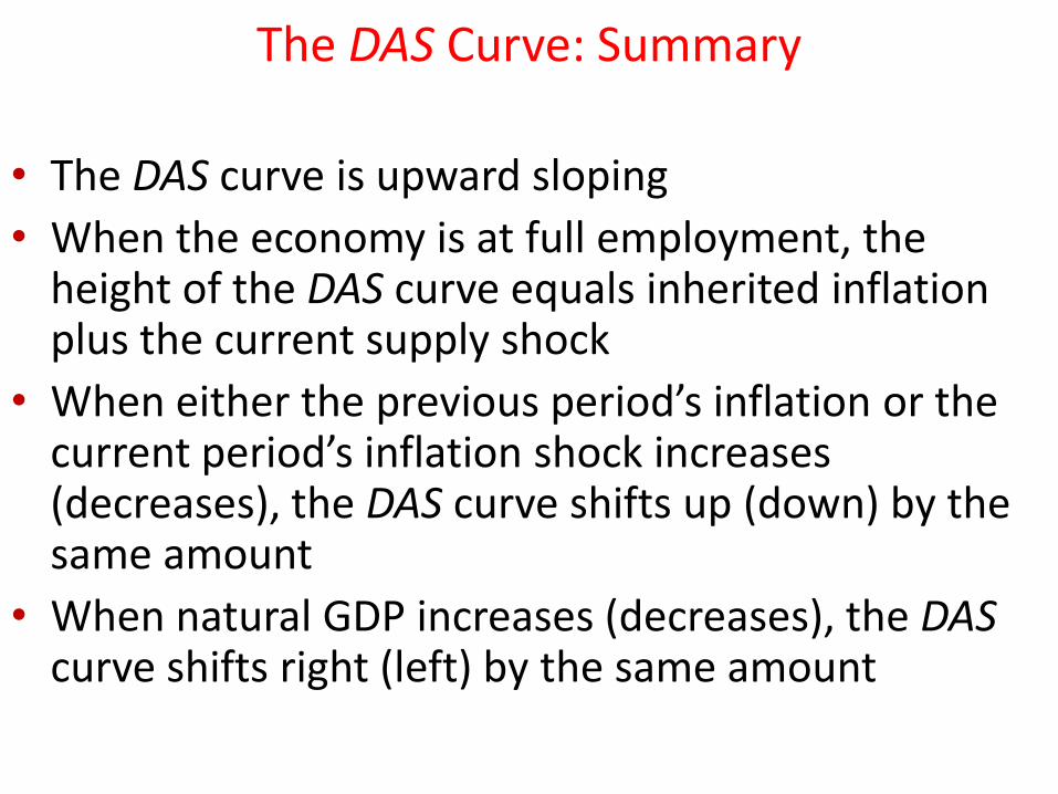
The DAS Curve: Summary
• The DAS curve is upward sloping
• When the economy is at full employment, the height of the DAS curve equals inherited inflation plus the current supply shock
• When either the previous period’s inflation or the current period’s inflation shock increases (decreases), the DAS curve shifts up (down) by the same amount
• When natural GDP increases (decreases), the DAS curve shifts right (left) by the same amount
DAD-DAS: 5 Equations
• The supply side - DONE
– 1. Phillips Curve
– 2. Adaptive Expectations
• The Demand Side
– 3. The Demand Equation
– 4. Fisher Equation
– 5. Monetary Policy Rule

IS Curve = Demand Equation
• The IS curve can simply be renamed the Demand Equation curve
rt
Yt
rt
Yt
IS
ttttrYY )(
ε

The Demand Equation
tttt rYY )(
Real GDP
Natural (or long-run or potential) Real GDP
Parameter representing the
response of demand to the real
interest rates
Real interest
rate
Natural (or long-run)
Real interest rate
Demand shock, represents
changes in G, T, C0, and I0

The Demand Equation
tttt rYY )(
α > 0
Assumption: ρ > 0; although the real interest rate can be negative, in the long run people will not lend their
resources to others without a positive return.
Positive when C0, I0, or G is higher than usual or T is lower than usual.
Assumption: There is a negative relation between output (Yt) and interest rate (rt). The justification is the same as for the IS curve

DAD-DAS: 5 Equations
• Phillips Curve
• Adaptive Expectations
• Demand Equation
• Fisher Equation
• Monetary Policy Rule

The Real Interest Rate: The Fisher Equation
1t t t tr i E
nominal
interest
rate
expected
inflation rate
ex ante
(i.e. expected)
real interest
rate
The real interest rate is the inflation-adjusted interest rate. To adjust the nominal interest rate for inflation, one must simply subtract the expected inflation rate during the duration of the loan (the true future inflation is not known )

The Real Interest Rate: The Fisher Equation
• Using adaptive expectations:
• We get the following relationship:
tttE
1
tttir
DAD-DAS: 5 Equations
• Phillips Curve
• Adaptive Expectations
• Demand Equation
• Fisher Equation
• Monetary Policy Rule

Monetary Policy Rule
• The fifth and final main assumption of the DAD-DAS theory is that
– The central bank sets the nominal interest rate
– and, in setting the nominal interest rate, the central bank is guided by a very specific formula called the monetary policy rule

The Nominal Interest Rate: The Monetary-Policy Rule
*
tttti
Nominal interest rate, set each period by the central bank
Current inflation rate
Natural real interest rate
Parameter that measures how strongly the central bank responds to the inflation gap
Inflation Gap: The excess of current inflation over the central bank’s inflation target

The Nominal Interest Rate: The Monetary-Policy Rule
• The Central Bank has a desired (target) inflation rate
• It adjusts the interest rate in such a way, as to reach this target
• When current inflation is equal to the target inflation, nominal interest rate is equal to:
tt
i *

The Dynamic Aggregate Demand Curve
( )t t t tY Y r
Fisher equation with adaptive expectations
tttir
( ) t t t t tY Y i
Start with the Demand Equation:
*
tttti
monetary policy rule
ttttt
YY
*)(

The Dynamic Aggregate Demand Curve
ttt
ttt
AYY
YY
*)(
*)(

The Dynamic Aggregate Demand Curve
DAD slopes downward: When inflation rises, the central bank raises the real interest rate, reducing the demand for goods and services.
Y
π
DADt Note that the DAD equation has no dynamics in it: it only shows how simultaneously measured variables are related to each other
tttAYY *)(

The Dynamic Aggregate Demand Curve
Y
π
DADt=1
*
1t
tY
When the central bank’s target inflation rate increases (decreases) the DAD curve moves up (down) by the exact same amount.
DADt=2
Note how monetary policy is described in terms of the target inflation rate in the DAD-DAS model
tttAYY *)(
*
2t
Assume: ε=0

The Dynamic Aggregate Demand Curve
Y
π
DADt=1
*
t
1tY
When the natural rate of output increases (decreases) the DAD curve moves right (left) by the exact same amount.
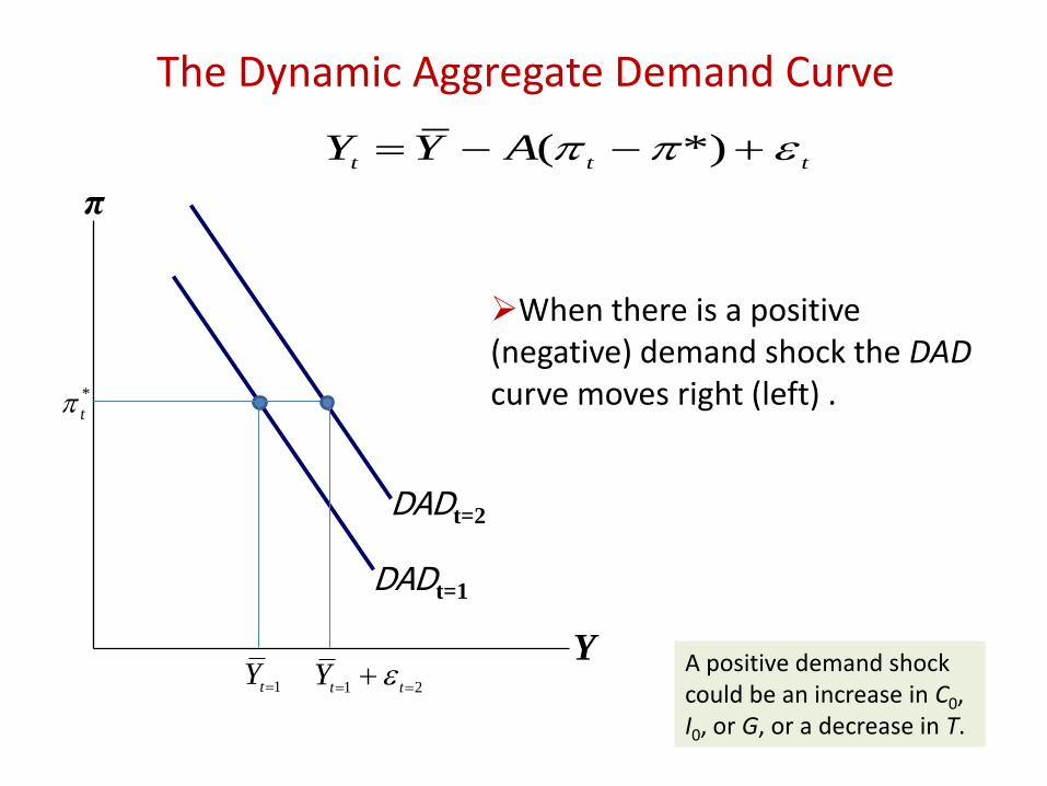
When there is a positive (negative) demand shock the DAD curve moves right (left) .
A positive demand shock could be an increase in C0, I0, or G, or a decrease in T.
DADt=2
2tY
tttAYY *)(
The Dynamic Aggregate Demand Curve
Y
π
DADt=1
*
t
1tY
When there is a positive (negative) demand shock the DAD curve moves right (left) .
A positive demand shock could be an increase in C0, I0, or G, or a decrease in T.
DADt=2
21
ttY
tttAYY *)(

The Dynamic Aggregate Demand Curve
Y
π
The DAD curve shifts right (or up) if: 1. the central bank’s target
inflation rate goes up, 2. there is a positive demand
shock, or 3. the natural rate of output
increases. DADt1
DADt2
tttAYY *)(

The DAD Curve: Summary
• The DAD curve is downward sloping
• When the central bank’s target inflation rate increases (decreases), the DAD curve shifts up (down) by the same amount
• When natural GDP increases (decreases), the DAD curve shifts right (left) by the same amount
• When the demand shock increases (decreases), the DAD curve shifts right (left)

DAS and DAD Equations
• Note that there are two endogenous variables—Yt and πt—in these two equations
• Therefore, we can solve for the equilibrium values of Yt and πt
ttttt
YY 1
DAS
DAD ttt
AYY *)(

Solution
ttttt
ttttt
tttttt
tttttt
AA
AYY
AYYA
AAYYAAYY
YYAYY
)1(*)(
)1(
*)()1(
*
*)(
1
1
1
1

The model’s variables and parameters
• Endogenous variables:
tY
tr
t
1t tE
ti
Output
Inflation
Real interest rate
Nominal interest rate
Expected inflation

The model’s variables and parameters
• Exogenous variables:
• Predetermined variable:
tY
*
t
t
t
1t
Natural level of output
Central bank’s target inflation rate
Demand shock
Supply shock
Previous period’s inflation

The model’s variables and parameters
• Parameters:
Responsiveness of demand to
the real interest rate
Natural rate of interest
Responsiveness of inflation to
output in the Phillips Curve
Responsiveness of i to inflation
in the monetary-policy rule

Long-Run Equilibrium
π*
Y
π
DAS
Y
DAD
A
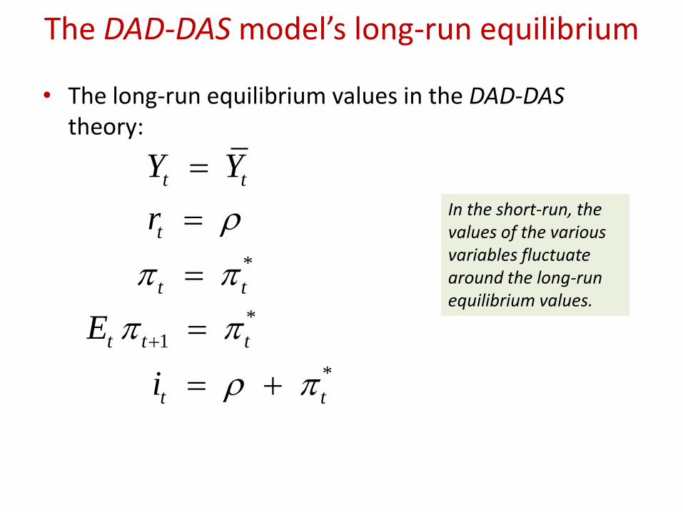
The DAD-DAS model’s long-run equilibrium
• The long-run equilibrium values in the DAD-DAS theory:
t tY Y
tr
*
t t *
1t t tE
*
t ti
In the short-run, the values of the various variables fluctuate around the long-run equilibrium values.