A DSGE Model on Unemployment in the Philippines: Assessing the Impact of Fiscal and Monetary Policies Academic Year 2015, Summer Semester

Submitted by: Tatum Blaise Pua Tan Advisers: Professor Hiroaki Miyamoto, Professor Kenichi Ueda, and Professor Takeki Sunakawa Graduate School of Public Policy The University of Tokyo

ABSTRACT

This paper is an antecedent application of the DSGE framework that incorporates labor search theory to the Philippines, in an effort to examine and analyze the impact of expansionary fiscal and monetary shocks on output and unemployment. Results of the calibrated baseline model show that both fiscal and monetary shocks cause output expansion and an increase in vacancies, leading to a decline in the unemployment rate. A fiscal shock leads to a rise in the hours worked and a fall in investment, consumption, and wage rates, while a monetary shock results in a rise in all listed variables. It is also noted that the fiscal shock exhibits more persistent effects on the economy and labor market than a monetary one. The simulations are also able to identify the potential areas for enhancement in the calibrated model, in order to better capture the impact of shocks on output and unemployment in the future. Overall, the current model allows us to advance our understanding of unemployment dynamics in the Philippines, and assess the effectiveness of policies in stimulating growth and addressing unemployment in the country.

Keywords: DSGE, Labor Search, Unemployment in the Philippines

ACKNOWLEDGEMENTS

I

I would like to express my utmost gratitude to Professor Hiroaki Miyamoto, for generously imparting his knowledge and extending ceaseless support during the making of this research paper, until its conclusion. I further extend my most sincere thanks to my supervisor, Professor Kenichi Ueda, for providing his expertise and views on the subject. My gratitude also goes to Professor Takeki Sunakawa for his keen guidance and valuable insights, which really helped improve my work during the process. My heartfelt appreciation goes out to friends, colleagues, and classmates, who were my proofreaders, data and technical support providers, and my cheerleaders! I also want to say thank you to my family for their unwavering support and encouragement. Lastly, I am grateful to the Almighty for all the divine intervention that has given me the will and strength to complete this coursework.

TABLE OF CONTENTS

1 Introduction ...................................................................................................................... 1

2 Review of Related Literature ...................................................................................... 4

3 The Model .......................................................................................................................... 7 3.1 The Labor Market ................................................................................................................. 7 3.2 Households ............................................................................................................................. 8 3.3 Intermediate Goods Firm ................................................................................................10 3.4 Retailers and Price Setting ..............................................................................................11 3.4 Wage and Hours Bargaining ...........................................................................................13 3.5 Monetary/Fiscal Policies and Closing the Model ....................................................13

4 Calibration ...................................................................................................................... 15

5 Impulse Response Functions and Analysis ......................................................... 17 5.1 Fiscal Shock ..........................................................................................................................17 5.2 Monetary Shock ...................................................................................................................18

6 Conclusion ...................................................................................................................... 20

References .......................................................................................................................... 25

Tables Table 1: Policy Rate Reductions by the BSP during the Crisis ............................... 3

Table 2: Calibration of Parameters ................................................................................... 15

Figures Figure 1: Cross-country GDP Growth .................................................................................. 1

Figure 2: Cross-country Unemployment Rate ................................................................ 1

Figure 3: Impulse Responses to a Fiscal Shock.......................................................... 18

Figure 4: Impulse Responses to a Monetary Shock .................................................. 19

Figure 5: Cross-country Labor Force Expansion ........................................................ 20

Figure 6: Real Minimum Wage, NCR ................................................................................. 20

Appendices Appendix 1: Steady State Conditions ............................................................................... 22

Appendix 2: Log-linear Equilibrium Conditions ........................................................ 23

1

1 Introduction The Philippines has displayed a remarkable economic performance in recent years, exhibiting resilience amid a series of global economic downturns, as seen in Figure 1. This is mainly on account of the country’s sound macroeconomic fundamentals, supported by expansionary fiscal and monetary policies undertaken by the authorities to keep the economy afloat during these crisis periods. However, robust economic growth has not progressed as swiftly as expected in terms of making a definite impact on the labor market. This has prompted some economists to dub it, a “jobless growth.” It may be noted that the Philippines has registered the highest unemployment rate relative to its peers in the region, hovering at seven to eight percent for almost a decade, as shown in Figure 2. Hence, the persistently high rate of unemployment continues to be one of the core issues confronting the nation, and a significant challenge for policy makers. After redeeming itself from being the region’s economic laggard, the Philippines now faces rising pressure to successfully translate “growth” into a measurably lower rate of unemployment. Despite the central role unemployment plays in the Philippine economy, its inclusion remains limited in academic papers employing contemporary empirical models. Thus, the motivation of this research is twofold. First, this research intends to set the stage for the use of Dynamic Stochastic General Equilibrium (DSGE) models that integrate labor search theory to study unemployment, which to my knowledge is the first of such undertaking based on the Philippines. Labor search theory is

0

2

4

6

8

10

12

2005 2006 2007 2008 2009 2010 2011 2012 2013

Figure2:Cross-CountryUnemploymentRate

Indonesia Korea,Republicof Malaysia

Philippines Thailand VietNam

Figure 2: Cross-country GDP Growth

-2

0

2

4

6

8

10

2005 2006 2007 2008 2009 2010 2011 2012 2013

Figure1:Cross-CountryGDPGrowth

Indonesia Korea,Republicof Malaysia

Philippines Thailand VietNamFigure 1: Cross-country Unemployment Rate

Note: In 2005, the National Statistical Coordination Board (NSCB) implemented the inclusion of a third criterion that is the person must also be available for work—in paid or self-employment—during the basic survey reference period. In addition, a six-month cut-off period for the job search of the discouraged workers was imposed. Source: www.adb.org

2

a popular model in evaluating structural unemployment due to the mismatch between heterogeneous workers and jobs. According to Rocheteau (2006), the theory of unemployment has three key components: wage setting, posting job vacancies, and the matching of jobs and workers. In order to better analyze unemployment, it is essential to assimilate these elements into the framework. This research adopts a highly stylized model by combining papers by Kato and Miyamoto (2012) and Kuo and Miyamoto (forthcoming). However, the fairly prefatory nature of this work warrants the adoption of a relatively simplified calibrated model. I believe that this study can serve as a sound groundwork for future development of more powerful models encompassing unemployment dynamics. To shed light on the dynamics involved in the theory of unemployment, Rocheteau (2006) provides the following explanation of the key elements. First, firms and their employees undergo a bargaining process to determine the wages, wherein the party with more leverage gains the bigger fraction of the surplus. Second, posting job vacancies and hiring new workers not only takes time, but also entails costs like advertising and evaluating applicants. Therefore, firms will only hire employees if the benefits outweigh the costs. Lastly, the matching function depicts the relationship between the number of unemployed, the number of vacancies, and the number of jobs created. As the pool of unemployed people expands, job seekers will experience a congestion effect that adversely affects their probability of finding a job successfully. This shows that the matching mechanism is neither smooth nor instantaneous. The second motivation of this research is to broaden the analysis of the impact of expansionary fiscal and monetary policies not only on growth, but also on unemployment. Like many other countries during the recent global crisis, the Philippine government launched its own stimulus package—the Emergency Resiliency Plan (ERP) amounting to P330 billion pesos (4.1 percent of GDP)— in an effort to stimulate the economy (Doraisami, 2011). 1 Although the specific channels where these funds were directed substantially influenced the stimulus’ effectiveness, this study takes a more macroeconomic approach by examining the broader impact of fiscal expansion on the economy and the labor market. While some DSGE papers in the Philippines have already examined the effect of fiscal spending using New Keynesian models, the analysis on the labor market have been limited to labor demand and hours worked (see McNelis, Glindro, Co, and Dakila, 2009 and Majuca, 2011). Therefore, to provide the link that will enable the current analysis to extend to unemployment, this research incorporates the Mortensen-Pissarides (1994, as in Kato and Miyamoto, 2012) search and matching model into the existing framework. Furthermore, I have extended my assessment to include the impact of a negative monetary shock on the economy and unemployment. It may be noted that unlike

1 Doraisami (2001) details the ERP package as follows: P160 billion of national spending on community-level infrastructure projects and social protection measures; P100 billion to finance extra-budgetary infrastructure projects and large infrastructure projects; P30 billion for new and temporary additional benefits to SSS, GSIS and PhilHealth; and P40 billion in income tax cuts.

3

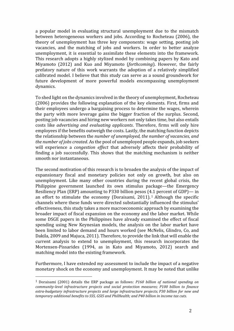
the US Federal Reserve Bank which has the statutory objectives to not only ensure stable prices but also facilitate maximum employment, the Bangko Sentral ng Pilipinas’ (BSP) sole objective in conducting monetary policy under an inflation-targeting framework is price stability. It should be noted however, that during the recent global downturn the BSP implemented a series of policy rate reductions to aid the weakening economy, as shown in Table 1. This brought the overnight reverse repurchase rate (RRP) and the repurchase rate (RP) down to 4.0 and 6.0 percent, respectively (Guinigundo, 2009). While the move was directly intended to stave off economic slowdown by stimulating business and household activities, such an expansion could have a spillover effect into the labor market. Employing the same calibrated DSGE model, this study examines the effect of a one standard deviation monetary shock to the economy and the unemployment rate. The results of the study show that a shock on fiscal spending leads to a decline of the unemployment rate attributable to the expansion of output and increase in vacancies posted by firms. A fiscal shock also leads to a rise in hours worked but at the same time, results in a fall in investment, consumption, and wage rates. Similarly, an expansionary monetary policy shock lowers the unemployment rate. However, the impact of the shock on some variables, particularly the rise in output, investment, hours worked, and vacancies, appear to be transitory. In addition, the simulations in the calibrated baseline model enable the identification of key areas for improvement in the framework to better capture the effect of monetary and fiscal shocks on the economy. Overall, a fiscal shock exhibits more persistent effects on the economy and the labor market than a monetary shock. The rest of the paper is organized as follows: Section II provides a review of the related literature; Section III presents the estimated DSGE model, providing details of the functions used for the labor market, households, firms, and authorities; Section IV covers the calibration; Section V presents and analyzes the impulse response functions; and Section VI concludes.

Table 1: Policy Rate Reductions by the BSP during the Crisis

Source: Guinigundo, Diwa C. (2009). The Impact of the Global Financial Crisis on the Philippine Financial System – An Assessment. Bank for International Settlements (BIS) Papers No. 54, 332.

4

2 Review of Related Literature There are already a number of research papers employing DSGE in the Philippines, including the work by McNelis, et al. (2009), which develops a small open economy DSGE model for the Philippines to assess the impact of fiscal and monetary policies in the economy. Their results indicate that a 25bps reduction in the RRP rate leads to higher prices and inflation as well as an initial exchange rate depreciation, translating to a modest output growth. This is fuelled by the increased production in the tradable sector, which raises labor demand. However, the rise in price level prevails over the depreciation, causing a real exchange rate appreciation, which in turn causes a bigger output contraction later on. Meanwhile, a fiscal stimulus amounting to one percent of GDP initially raises output, mainly propelled by the non-tradable sector, translating to higher labor demand. Likewise, nominal wages and prices increase, feeding into inflation, which in turn provides an impetus to raise interest rates. This eventually leads to a real exchange rate appreciation and a deterioration of the current account balance, thereby lowering output and inflation. Overall, the research finds that the effect of monetary policy is more pronounced on the tradable sector, while the effect of fiscal policy is more prominent on the non-tradable sector. Although their research covers the impact of both policy actions, it does not delve into the specifics of the labor market reasonably. Hence, my study will focus on this untapped area. Similarly, Majuca (2011) develops a medium-scale closed economy DSGE model for the Philippines using a multi-period sample (pre- and post-IT) to evaluate credibility gains from inflation targeting, which the BSP adopted in 2002. The paper includes a significantly more comprehensive set of frictions, namely: investment adjustment costs, habit formation, price and wage rigidities, variable indexation, fixed costs, as well as price and wage indexation. Empirical results of the model find that an increase in the BSP’s policy decreases output, consumption, investment, wages, and inflation, while increasing the interest rate. The study also simulates an exogenous spending shock, corresponding to a demand shock, which covers shocks to both government spending and net exports. An increase in this exogenous spending raises output, hours worked, wages, and inflation, but causes consumption, investment, and BSP policy rates to fall. In addition, the research concludes that the Philippine economy is more stable with lower risk aversion in the post-IT era. Among the relatively early works that incorporate elements of labor market matching functions in DSGE models is that of Walsh (2003), which examines the role of labor market matching function and price stickiness in influencing the impact of monetary shocks, in the form of money growth, to the economy. The representative household in his model consists of workers and shoppers facing a utility maximization problem with two constraints—the resource constraint and a cash-in-advance constraint (i.e. income in period t cannot be used for consumption until t+1). This allows the nominal interest rate to influence the discounted value current production, and subsequently output and employment as well. The labor search dynamics and price stickiness are integrated through the inclusion of a wholesale sector, where matched firms and workers generate

5

output, and a monopolistically competitive retail sector facing sticky prices. The study finds that under sticky prices, the expansionary monetary shock increases output, employment, and job creation while at the same time, decreases job destruction reducing the number of job seekers. In tackling a relatively similar issue to the above research, Galí (2010) simulates the impact of a contractionary monetary policy shock to the US economy, using a Taylor-type interest rate rule with an exogenous policy shifter. The paper extends the New Keynesian model to distinctly incorporate labor market frictions and unemployment, as well as highlights the effect of the presence of price and wage stickiness on the impact of the shocks. The model offers two alternative wage settings—employing Nash bargaining to represent the case of flexible wages and incorporating staggered nominal wage setting à la Calvo (1983) for sticky wages. Results in Galí’s calibrated model show that a monetary policy shock with price and wage stickiness leads to a fall in output, inflation, and employment as well as an increase in unemployment. Although, the decline in inflation is more muted in the case of sticky wages. Galí also finds that the effect of labor market frictions to the response of the economy’s equilibrium dynamics, in the context of an economy with rigidities and Taylor-rule monetary policy to shocks, is quite limited. Lastly, the study covers comparisons on the optimal monetary policy design with simulated technology shocks. However, this is outside the scope of my research. Faccini, Millard, and Zanetti (2011) likewise employ a model that integrates matching frictions as well as á la calvo price and wage rigidities to the New Keynesian framework using UK data. They reckon that the introduction of these frictions enhanced the robustness of their model, facilitating a better fit with the data. Sans wage stickiness, they find that a one standard deviation monetary policy shock results in a decline in output, consumption, investment, price inflation, employment, hours worked, unit labor costs, and vacancies. While the trend of the variables appears to be generally the same in the case of sticky wages, except for wage inflation and unit labor costs, the magnitude varies. The model also offers an estimate on vital structural variables, which helps shed light on the transmission mechanism of shocks in light of wage rigidities, and the key economic factors driving the economic fluctuations in the country. However, their study shows that wage rigidities are extraneous in the inflation dynamics due to the offsetting effect of unit labor costs and search costs. It may also be noted that unlike my study which employs a Nash wage bargaining system, their study employs a sharing rule wherein the fraction of the total surplus owing to the workers corresponds to their bargaining power, following Thomas (2008, as in Faccini, et al., 2011). Mixed conclusions can be drawn from the different literature on the impact of fiscal shocks on unemployment. On one hand, Kato and Miyamoto (2012) find that fiscal expansion improves labor market condition in Japan. Their research is related to that of Monacelli, Perotti and Trigari (2010, as cited in Kato Miyamoto, 2012), which studies the impact of fiscal policy in the US, but differs as it allows adjustment in in the intensive margin of labor. Kato and Miyamoto (2012) use both a structural VAR (SVAR) model and a dynamic general equilibrium model with search and matching frictions akin to Mortensen and Pissarides (1994, as

6

cited in Kato and Miyamoto, 2012). Using the SVAR model, they find that fiscal expansion decreases unemployment and increases employment, and correspondingly improves the job finding rate while easing the job separation rate. Although the DSGE model finds similar patterns on the effect of government spending on labor market variables (i.e. increases in output, hours worked per worker and vacancies, as well as decline in unemployment rate), the magnitude of the impact differs. While this is one of the materials that this paper draws from, my research employs an expanded resource constraint faced by the household to include government bond holdings, at the same time extends the analysis to include the monetary sector. On the other hand, Mayer, Moyen, and Stähler (2010) find that a fiscal shock could increase unemployment, contingent upon the persistence of the fiscal shock and the kind of household. They reckon that a transitory fiscal expansion is likely to be ineffective if the firms’ hiring decisions are more forward looking. In other words, firms could benefit from creating jobs as the marginal profit of a worker rises during the period, but the new matches are unlikely to survive. Moreover, their model differs from the previously cited research as it differentiates between optimizing households that save and liquidity constrained households that consume all their labor income, whose consumption behavior run in opposite directions following an augmented fiscal spending. They infer that incentive for the latter to put in more hours diminishes because the marginal utility of consumption declines relative to the marginal disutility of hours working. Therefore if liquidity constrained households dominate the market, fiscal expansion results in an increase in unemployment notwithstanding the persistence of the shock.

7

3 The Model This research offers a precursor application of a DSGE framework incorporating labor search theory in the New Keynesian model to the Philippines, in order to examine and analyze the impact of fiscal and monetary shocks on output and unemployment. The inclusion of labor search theory enables the model to better capture unemployment dynamics by accounting for the fact that hiring and job seeking both entail costs and time, rather than the idea of workers seamlessly flowing in and out of the market (Mortensen and Pissarides, 1994 and Pissarides, 2000, as cited in Walsh, 2003). The methodology fundamentally combines the models by Kato and Miyamoto (2012) and Kuo and Miyamoto (forthcoming) to develop a more straightforward model. The economy in this study consists of the households, competitive intermediate firms, monopolistically competitive retailers, and both monetary and fiscal authorities. Using this mix of market agents allows policy analysis to extend to cover the impact of monetary and fiscal policies on output and unemployment.

3.1 The Labor Market As mentioned earlier, firms and workers undergo a laborious search process compelled by the frictions inherent in the market, which otherwise would allow perfect movements in the labor flow. This paper integrates this condition in the general model by utilizing the following standard matching function of the Cobb-Douglas form

𝑚𝑡 = 𝑀𝑡𝑢𝑡𝜉

𝑣𝑡1−𝜉

. where 𝑚𝑡 is the number of matches, 𝑢𝑡 is the number of job-seekers, 𝑣𝑡 is the number of vacancies posted by the intermediate firms, and 0 < 𝜉 < 1 denotes the elasticity of the matching function with respect to unemployment. Moreover, the time-varying matching efficiency, 𝑀𝑡, follows the stochastic process

log 𝑀𝑡 = (1 − 𝜌𝑀) log 𝑀 + 𝜌𝑀 log 𝑀𝑡−1 + 휀𝑀,𝑡, 휀𝑀,𝑡~𝑁(0, 𝜎𝑀2 ).

During each period, the probability that a vacancy is filled is represented by 𝑞𝑡 =

𝑚𝑡

𝑣𝑡⁄ = 𝑀𝑡휃𝑡

−𝜉 , while the probability that a job seeker is employed is

represented by 𝑝𝑡 = 𝑚𝑡

𝑢𝑡⁄ = 𝑀𝑡휃𝑡

1−𝜉 . The labor market tightness is then

denoted by 휃𝑡 =𝑣𝑡

𝑢𝑡⁄ .

At the beginning of a period t, intermediate firms search for new hires by posting vacancies 𝑣𝑡 , at the same time, 𝑢𝑡unemployed workers look for jobs. This process results in new matches 𝑚𝑡. New hires are assumed to start working and become productive immediately within the same period. Consequently, a constant fraction of workers loses their job at the end of each period and will not be able to search for a new one until the following period t +1. Thus, the evolution of employment is as follows

𝑛𝑡 = (1 − 𝑠)𝑛𝑡−1 + 𝑚𝑡 = (1 − 𝑠)𝑛𝑡−1 + 𝑝𝑡𝑢𝑡 = (1 − 𝑠)𝑛𝑡−1 + 𝑞𝑡𝑣𝑡 . (1)

8

Meanwhile, the number of job seekers is represented by

𝑢𝑡 = 1 − 𝑛𝑡−1 + 𝑠𝑛𝑡−1.

Hence, at time t, the number of employed workers is the sum of last period’s workers who were able to retain their jobs and the new hires/newly filled vacancies, while the corresponding number of unemployed workers is given by

𝑈𝑡 = 1 − 𝑛𝑡.

3.2 Households As in Kuo and Miyamoto (forthcoming), the representative household consists of a continuum of infinitely lived workers of measure one. A household member is either employed or unemployed. Employed members provide labor and earn wages, while the unemployed look for jobs. Every household consumes final goods, accumulates capital, acquires government bonds, and acts as shareholders of the intermediate goods firms. It is likewise assumed that the households decides on a utilitarian basis and thus, consumption is identical for each member regardless of employment status. Following Merz (1995, as in Kuo and Miyamoto, forthcoming), members of the representative household are provided perfect consumption insurance by one another against unemployment risks or income variability. The representative household’s lifetime utility function is akin to Kato and

Miyamoto (2012) and incorporates 𝛾𝑡 and 𝜒𝑡 , which denotes the preference and labor supply shocks, respectively. It is characterized by

𝔼0 ∑ 𝛽𝑡∞𝑡=0 [𝛾𝑡

𝐶𝑡1−𝜎

1−𝜎− 𝜒𝑡Φ𝑛𝑡

ℎ𝑡1+𝜇

1+𝜇] , (2)

where 𝛽 is the household’s subjective discount factor, 𝐶𝑡 is private consumption, ℎ𝑡 is the individual hours of work, Φ > 0 measures the disutility of labor supply, 𝜎 governs the degree of risk aversion or the inverse of the intertemporal elasticity of substitution, and 휇 is the inverse of Frisch elasticity of labor supply. The habit persistence perimeter is excluded selectively from the equation for simplicity.2 Note that the added preference shock 𝛾𝑡 and labor supply shock 𝜒𝑡follow a first-order autoregressive process with i.i.d.-normal error term

log 𝛾𝑡 = 𝜌𝛾 log 𝛾𝑡−1 + 휀𝛾,𝑡, 휀𝛾,𝑡~𝑁(0, 𝜎𝛾2),

log 𝜒𝑡 = 𝜌𝜒 log 𝜒𝑡−1 + 휀𝜒,𝑡, 휀𝜒,𝑡~𝑁(0, 𝜎𝛾

2).

2 McNelis, et al. (2009) assigns a lower value of habit persistence in their DSGE model for the Philippines vis-à-vis in the values used US studies, citing the Filipino consumers’ less habitual characteristic due to a higher degree of income uncertainty.

9

Moreover, given the capital stock 𝐾𝑡 in period t and depreciation rate 𝛿 , the household accumulates capital and achieves the desired level of capital 𝐾𝑡+1 in the following period by investing 𝐼𝑡. Employing evolution of capital by Faccini, et al. (2011), capital accumulation takes the form

𝐾𝑡+1 = (1 − 𝛿)𝐾𝑡 + Ψ𝑡𝐼𝑡, (3)

where Ψ𝑡is an investment shock, which follows a stochastic process

log Ψ𝑡 = 𝜌Ψ log Ψ𝑡−1 + 휀Ψ,𝑡, 휀Ψ,𝑡~𝑁(0, 𝜎𝛾2).

The representative household’s budget constraint is characterized by

𝐶𝑡 + 𝐼𝑡 + 𝑏𝑡+1 = 𝑛𝑡𝑤𝑡ℎ𝑡 + (1 − 𝑛𝑡)𝑧 + 𝑟𝑡𝐾𝐾𝑡 +

𝑅𝑡−1𝑏𝑡

𝜋𝑡+ 𝐷𝑡 − 𝜏𝑡, (4)

where 𝑏𝑡 is acquisition of government bond, 𝑛𝑡𝑤𝑡ℎ𝑡 is the total labor income earned by all employed workers, z is the unemployment benefits, 𝑟𝑡

𝐾is the rental rate of capital, 𝑅𝑡 is the nominal interest rate, 𝜋𝑡 is the price ratio, 𝐷𝑡 is the dividend receive by the households from the firms, and 𝜏𝑡 represents the lump-sum taxes paid to the government. Note that unemployment benefits do not necessarily refer to unemployment insurance from the government, rather it accounts for the outside opportunities available to the member who is not working (e.g. engaging in home production). The household maximizes its lifetime utility (2) subject to the employment constraint (1), capital accumulation equation (3), and the budget constraint (4), by choosing the optimal levels of 𝐶𝑡, 𝐼𝑡 , 𝐾𝑡+1, 𝑏𝑡+1, and 𝑛𝑡 . This yields the following first-order conditions:

휆𝑡 = 𝛾𝑡𝐶𝑡−𝜎;

휆𝑡 = 휆𝑡

𝐾Ψ𝑡 ;

휆𝑡𝐾 = 𝛽 [휆𝑡+1𝑟𝑡+1

𝐾 + 휆𝑡+1𝐾 (1 − 𝛿)] ; and

휆𝑡 = 𝛽 (휆𝑡+1

𝑅𝑡+1

𝜋𝑡+1 ),

where 휆𝑡 and 휆𝑡𝐾 are the Lagrange multipliers associated with the budget

constraint and the capital accumulation equation, respectively. To derive the marginal value of an employed worker to the household 𝒲𝑡, the

10

first-order derivative with respect to employment is taken

𝒲𝑡 = 𝑤𝑡ℎ𝑡 − 𝑧 − Φ𝜒𝑡

𝜆𝑡

ℎ𝑡1+𝜇

1+𝜇+ 𝛽 𝔼𝑡 [(1 − 𝑠)(1 − 𝑝𝑡+1)

𝜆𝑡+1

𝜆𝑡𝒲𝑡+1] , (5)

where 𝒲𝑡 = 𝜆𝑡

𝑛

𝜆𝑡 and 휆𝑡

𝑛 is the Lagrange multiplier associated with the constraint

pertaining to the evolution of employment. The equation implies that the marginal value of a job to an employed worker is equal to the wage net of unemployment benefits and the disutility of work plus the expected discounted value of being employed next period.

3.3 Intermediate Goods Firm The representative intermediate goods firm hires labor and rents capital from the households and produces homogeneous intermediate goods, which are then sold to the final goods firms in a competitive market. As in Kuo and Miyamoto (forthcoming), the intermediate goods firm produce output according to the following production function, which assumes a constant returns to scale production, whereby capital-labor ratio across all firms is the same,

𝑦𝑡 = 𝐴𝑡𝑘𝑡𝛼(𝑛𝑡ℎ𝑡)1−𝛼 (6)

where 0 < 𝛼 < 1 is the capital share and 𝐴𝑡 is an exogenous stochastic variable that captures neutral technology shocks

log 𝐴𝑡 = 𝜌A log 𝐴𝑡−1 + 휀A,𝑡, 휀A,𝑡~𝑁(0, 𝜎𝛾2).

The intermediate good firm maximizes the present value of its lifetime profit by choosing the optimal number of employees 𝑛𝑡 , number of vacancies 𝑣𝑡 , and level of capital 𝑘𝑡

𝔼0 ∑ [𝛽𝑡휆𝑡

휆0 (𝑥𝑡𝑦𝑡 − 𝑤𝑡𝑛𝑡ℎ𝑡 − 𝑟𝑡

𝐾𝑘𝑡 − 휅𝑣𝑡) ]

∞

𝑡=0

subject to the employment constraint (1) and production function (6). Since the households hold the equities of intermediate goods firms, said profits are estimated using the household’s discount factor in terms of marginal utility 휆𝑡. The

competitive price of intermediate goods is given by 𝑥𝑡, while the wage 𝑤𝑡 is set

through a bargaining process. The cost of posting a vacancy is denoted by 휅. The representative intermediate firm’s optimal decision with respect to capital

and employment, with a Lagrange multiplier 휆𝑡�� assigned to the latter, results in

the following first-order conditions

11

𝑟𝑡𝐾 = 𝛼

𝑥𝑡𝑦𝑡

𝑘𝑡 and

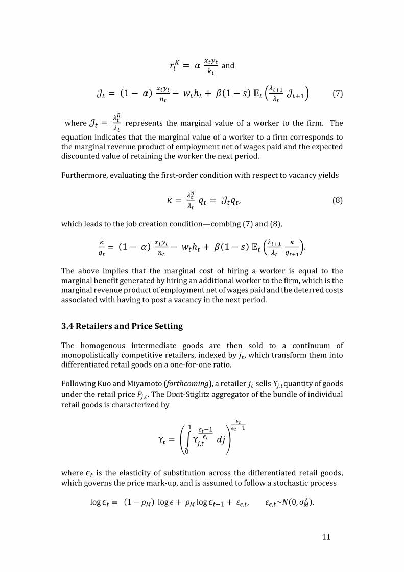
𝒥𝑡 = (1 − 𝛼) 𝑥𝑡𝑦𝑡

𝑛𝑡− 𝑤𝑡ℎ𝑡 + 𝛽(1 − 𝑠) 𝔼𝑡 (

𝜆𝑡+1

𝜆𝑡 𝒥𝑡+1) (7)

where 𝒥𝑡 = 𝜆𝑡

��

𝜆𝑡 represents the marginal value of a worker to the firm. The

equation indicates that the marginal value of a worker to a firm corresponds to the marginal revenue product of employment net of wages paid and the expected discounted value of retaining the worker the next period. Furthermore, evaluating the first-order condition with respect to vacancy yields

휅 = 𝜆𝑡

��

𝜆𝑡 𝑞𝑡 = 𝒥𝑡𝑞𝑡 , (8)

which leads to the job creation condition—combing (7) and (8),

𝜅

𝑞𝑡= (1 − 𝛼)

𝑥𝑡𝑦𝑡

𝑛𝑡− 𝑤𝑡ℎ𝑡 + 𝛽(1 − 𝑠) 𝔼𝑡 (

𝜆𝑡+1

𝜆𝑡

𝜅

𝑞𝑡+1).

The above implies that the marginal cost of hiring a worker is equal to the marginal benefit generated by hiring an additional worker to the firm, which is the marginal revenue product of employment net of wages paid and the deterred costs associated with having to post a vacancy in the next period.

3.4 Retailers and Price Setting The homogenous intermediate goods are then sold to a continuum of monopolistically competitive retailers, indexed by 𝑗𝑡, which transform them into differentiated retail goods on a one-for-one ratio. Following Kuo and Miyamoto (forthcoming), a retailer 𝑗𝑡 sells Υ𝑗,𝑡quantity of goods

under the retail price 𝑃𝑗,𝑡. The Dixit-Stiglitz aggregator of the bundle of individual

retail goods is characterized by

Υ𝑡 = (∫ Υ𝑗,𝑡

𝜖𝑡−1𝜖𝑡

1

0

𝑑𝑗)

𝜖𝑡𝜖𝑡−1

where 𝜖𝑡 is the elasticity of substitution across the differentiated retail goods, which governs the price mark-up, and is assumed to follow a stochastic process

log 𝜖𝑡 = (1 − 𝜌𝑀) log 𝜖 + 𝜌𝑀 log 𝜖𝑡−1 + 휀𝜖,𝑡, 휀𝜖,𝑡~𝑁(0, 𝜎𝑀2 ).

12

Each retailer 𝑗𝑡faces the following demand for its product

Υ𝑗,𝑡 = (𝑃𝑗,𝑡

𝑃𝑡)

𝜖𝑡

Υ𝑡 ,

where the cost minimizing aggregate price index 𝑃𝑡 is

𝑃𝑡 = (∫ 𝑃𝑗,𝑡1−𝜖𝑡1

0 𝑑𝑗)

1

1−𝜖𝑡 .

Á la Calvo (1983), it is assumed that only a fraction (1 − 𝜑)of retailers are able to re-optimize their prices each period. On one hand, for the jth retailer who is unable to re-optimize, its product price 𝑃𝑗,𝑡 conforms to the following partial indexation

scheme

𝑃𝑗,𝑡 = 𝜋𝑡−1

𝜄𝑝 𝜋1−𝜄𝑝𝑃𝑗,𝑡−1,

where 휄𝑝 represents the backward-looking parameter governing inflation,

𝜋𝑡−1 = 𝑃𝑡

𝑃𝑡−1 indicates the gross inflation rate in period 𝑡 − 1, and 𝜋 denotes the

steady-state inflation. On the other hand, the retailer who is able to re-optimize at time t chooses the optimal price ��𝑡 by evaluating the following profit maximization function subject to the subsequent aggregate demand function faced by each retailer 𝑗𝑡 under monopolistic competition

max��𝑡

𝔼𝑡 {∑(𝛽𝜑)𝑘 휆𝑡+𝑘

휆𝑡 [

(��𝑡ℱ𝑡,𝑘 − 𝑃𝑡+𝑘𝑥𝑡+𝑘)

𝑃𝑡+𝑘 Υ𝑡+𝑘]

∞

𝑘=0

}

Υ𝑡+𝑘 = ( ��𝑡ℱ𝑡,𝑘

𝑃𝑡+𝑘)

−𝜖𝑡

Υ𝑡+𝑘 .

The compound effect of partial indexation is described by ℱ𝑡,𝑘, wherein

ℱ𝑡,𝑘 = {∏𝑘=1𝑘 𝜋

𝑡+𝑘−1

𝜄𝑝 𝜋1−𝜄𝑝 𝑘 ≥ 1

1 𝑘 = 0.

The resulting first-order condition with respect to ��𝑡

𝔼𝑡 [∑(𝛽𝜑)𝑘 휆𝑡+𝑘(1 − 𝜖𝑡+𝑘) Υ𝑡+𝑘 (��𝑡ℱ𝑡,𝑘 − 𝜖𝑡+𝑘

𝜖𝑡+𝑘 − 1∏𝑡,𝑘𝑥𝑡+𝑘)

∞

𝑘=0

] = 0

13

where ��𝑡 = ��𝑡

𝑃𝑡 and ∏𝑡,𝑘 = {∏𝑘=1

𝑘 𝜋𝑡+𝑘

𝜄𝑝 𝑘 ≥ 1

1 𝑘 = 0. The equation

indicates that accounting for partial inflation indexation and the possibility of being stuck with this price in the succeeding periods, the optimal price selected by forward-looking re-negotiating firms should equal to the time-varying mark-up

𝜖𝑡+𝑘

𝜖𝑡+𝑘−1 (Christiano, Trabandt, and Walentin, 2010 and Faccini, et al., 2011).

3.4 Wage and Hours Bargaining Due to the presence of labor market frictions, the wage rate 𝑤𝑡 and hours of work per employee ℎ𝑡 are negotiated in a bilateral bargaining process between the workers and the intermediate firm so as to divide the surplus accordingly given the existing employment relations. Both variables are determined through Nash bargaining which aims to maximize the weighted average of the worker’s and the firm’s surplus

max𝑤𝑡ℎ𝑡

𝒲𝑡𝜂

𝒥𝑡1−𝜂

where 휂 ∈ (0,1) governs the worker’s bargaining power. Evaluating the first order conditions with respect to both wage and hours result in the following wage and hours supply equations

𝑤𝑡ℎ𝑡 = 휂 [(1 − 𝛼)𝑥𝑡𝑦𝑡

𝑛𝑡+ 𝛽 (1 − 𝑠)𝔼𝑡 (

휆𝑡+1

휆𝑡 휅휃𝑡+1)]

+ (1 − 휂) (𝑧 + Φ

1 + 휇

𝑥𝑡ℎ𝑡1+𝜇

휆𝑡)

(1 − 𝛼)2 𝑥𝑡𝑦𝑡

𝑛𝑡ℎ𝑡= Φ

ℎ𝑡𝜇

𝜆𝑡 𝜒𝑡 .

Kuo and Miyamoto (forthcoming) explains that the wage equation connotes that the wage rate is equal to the weighted sum of the firm’s gains, in terms of marginal revenue product and the continuation value of the worker, and the worker’s opportunity cost, consist of the unemployment benefits and the disutility of labor. Furthermore, the hours supply equation implies that the hours of work is established through the equalization of the marginal product of hours and the marginal rate of substitution between leisure and consumption.

3.5 Monetary/Fiscal Policies and Closing the Model The Central Bank employs a Taylor rule framework where the nominal interest rate is a function of the past interest rate 𝑅𝑡−1and deviations of inflation 𝜋𝑡 and

14

output Υ𝑡 from their respective steady state values—sans the subscript t. It is represented by

𝑅𝑡

𝑅= (

𝑅𝑡−1

𝑅)

𝜌𝑅

[(𝜋𝑡

𝜋)

𝜙𝜋

(Υ𝑡

Υ)

𝜙Υ

]1−𝜌𝑅

휁𝑚𝑝,𝑡−1,

where the parameter 𝜌𝑅 denotes the interest rate smoothing while 𝜙𝜋 and 𝜙Υ govern the response of the Central Bank to deviations of inflation and output from their steady-state values. Moreover, monetary policy shocks 휁𝑚𝑝,𝑡 are i.i.d and is

raised to negative one to generate an expansionary shock. Meanwhile, the spending aspect in the fiscal equation consists government consumption 𝐺𝑡, bond interest payments, and unemployment benefits, while the financing side includes lump-sum taxes and bond issuances.

𝜏𝑡 + 𝑏𝑡+1 = 𝐺𝑡 +𝑅𝑡

𝜋𝑡𝑏𝑡 + (1 − 𝑛𝑡)𝑧.

Note that 𝐺𝑡 follows a stochastic process characterized as

log ��𝑡 = 𝜌𝐺 log ��𝑡−1 + 휀𝐺,𝑡, 휀𝐺,𝑡~𝑁(0, 𝜎𝐺2),

where ��𝑡 ≡ (𝐺𝑡− 𝐺)

Υ is the percentage deviation of government spending from

the steady state output level and 𝜌𝐺 is the persistency of government consumption. Moving ahead, in the market clearing condition, the demand for capital goods by the intermediate firms must equal the capital supplied by the households, i.e., 𝑘𝑡 =𝐾𝑡. To close the model, the resource constraint of the economy is given by

Υ𝑡 = 𝐶𝑡 + 𝐼𝑡 + 𝐺𝑡 + 휅𝑣𝑡 .

15

4 Calibration Calibration is a commonly used method in DSGE literature in estimating parameters. It provides a good indication of the model’s capability and allows the assessment of the implications of different policy scenarios (Mutschler, 2014). This section explains the calibration of parameters for the baseline model in order to match certain elements of the Philippine economy, presented in Table 2. Following Kuo and Miyamoto (forthcoming), the elasticity of matching function 𝜉 is set at 0.6, a little higher than the conventional 0.5 in some literature. The exogenous separation rate s approximated at 7.87 percent is derived using the average of the data on separation rate for the Metro Manila/National Capital Region from the Labor Turnover Statistics of the Bureau of Labor and Employment Statistics covering the period 2003:Q1-2014:Q4. Similarly, the steady state unemployment rate u at 7.32 percent is a simple average of the unemployment rate from 2005:Q1-2014:Q4 from the Labor Force Survey published by the National Statistics Office (NSO).

Table 2: Calibration of Parameters

Parameter Notation Value Elasticity of matching function 𝜉 0.6 Exogenous separation rate s 0.0787 Steady state unemployment rate u 0.0732 Discount factor 𝛽 0.99

Degree of risk aversion 𝜎 2 Inverse of Frisch elasticity 휇 0.25 Unemployment benefits z 0.15 Depreciation rate 𝛿 0.05 Capital input elasticity of output in the Cobb-Douglas production function

𝛼 0.36

Cost of posting a vacancy 휅 0.05 Calvo Parameter 𝜑 2/3 Steady state gross inflation rate 𝜋 1 Backward-looking parameter governing inflation

휄𝑝 0.5

Elasticity of demand to market share 𝜖 11 Bargaining power 휂 0.6 Steady state hours h 1/3 Steady state government spending to output ratio

g/y 0.116

Taylor Rule Parameters 𝜌𝑅 , 𝜙𝜋 and 𝜙Υ 0.9, 1.5, 0.1 Autoregressive parameter 𝜌𝐺 0.8

Standard deviations 𝜎𝐺 , 𝜎�� 0.1

16

The discount factor 𝛽 is set at 0.99, as in most literature, implying an annual real interest rate of 4.0 percent. The degree of risk aversion is fixed at two, following the DSGE literature on emerging market economies (EMEs) (see Boz, Durdu, and Li, 2012 and Epstein and Shapiro, 2014). Similarly, McNelis, et al. (2009) reckon that the parameter is usually greater than 1.5 for EMEs. Consistent with McNelis, et al. (2009), labor supply elasticity is placed at 0.25, implying a Frisch elasticity of four. Since, there is no available data/literature to evaluate the value of unemployment benefits and considering the absence of unemployment insurance from the government in the Philippines, the study sets the parameter z at 0.15, which is lower than that of Kato and Miyamoto (2012) at 0.20. The depreciation rate 𝛿 is set at 0.05 percent, since developing countries are supposed to have higher depreciation rate because of the relatively modest maintenance capability (Bu, 2006 as cited in Majuca, 2011). With reference to Majuca’s (2011) paper, the selected depreciation rate lies between the Majuca’s calculated implied depreciation using firm-level data at 0.0575 percent per quarter and the estimate used in his research at 0.04 percent per quarter. Following Boz, et al. (2012), whose study examines the role of labor market frictions in the business cycles experienced by EMEs, the capital input elasticity of output in the Cobb-Douglas production function 𝛼 is estimated at 0.36. As in Kuo and Miyamoto (forthcoming), the cost of posting a vacancy, the Calvo parameter, and the elasticity of demand to market share are set at 0.05, 2/3, and 11, respectively. The latter translates to a steady state profit margin of 10 percent for the retailers. The steady state gross inflation rate is set at one, implying a zero inflation rate. Consistent with Majuca (2011) the backward-looking parameter governing inflation 휄𝑝 is estimated at 0.5.

Employing Kuo and Miyamoto’s (forthcoming) estimates for the worker’s bargaining power and steady state hours of work per worker, 휂 and h are set at 0.6 and 1/3, respectively. The wage bargaining arrangement between the relevant countries could share a common feature in a sense the workers’ bargaining power is relatively constrained. Brooks (2002) explains that the minimum wage in the Philippines is set by the Regional Tripartite Wages and Productivity Boards and representatives from the government, businesses, and labor unions and then reviewed by the National Wages and Productivity Commission to ascertain that the criteria for setting the minimum wage are met. The said study asserts that while the government advocates an enterprise level collective bargaining for wage setting, the coverage remains limited. In addition, the research mentions that union representatives deem that some employers do not regard them as collaborators in the pursuit of improving labor productivity and working conditions. Meanwhile, the Taylor Rule parameters 𝜌𝑅 , 𝜙𝜋 and 𝜙Υ follow that of Kuo and Miyamoto (2009) at 0.9, 1.5, 0.1, respectively. These values are also close to Majuca’s (2011) conjecture of the Central Bank’s monetary reaction function during post inflation targeting period and his prior on the interest rate feedback from changes in the output gap. Lastly, the first order autoregressive parameter of the exogenous disturbances on government spending is set equal to 0.8 while the standard deviations for both shocks are set equal to 0.1.

17

5 Impulse Response Functions and Analysis

5.1 Fiscal Shock This section analyzes the impulse responses of selected variables to a single period one standard deviation expansionary fiscal policy shock, especially unemployment, as shown in Figure 3. In the calibrated model, the fiscal shock results in higher output and expansion in the intensive margin. The maximal effect on output and hours worked are observed immediately on impact and eases in the following periods until they return to their steady state. This increase in spending is of course financed by higher taxes. The combined effect of higher taxes and lower wages generate a negative wealth effect, while the higher interest rate prompts a substitution effect. These factors compel the household to reduce consumption and increase labor supply. Similarly, the augmented fiscal spending pushes the interest rate up crowding out investments, which hits its trough in the second quarter.

The augmented government expenditure also causes a decline in the wages—the weighted sum of the firm’s marginal value of production (i.e. marginal product of employment and expected costs saved associated with not having to post a vacancy the next period) as well as the worker’s outside opportunities (i.e. unemployment benefits and disutility of work). While the shock supposedly puts an upward pressure on wages as it enhances the production value and intensifies the disutility of work from the increased work hours, the rise in government spending likewise boosts the shadow value of wealth, which mitigates the disutility of labor (Kuo and Miyamoto, 2015). This model finds that the impact of the latter is more pronounced.

The increase in interest rate follows the central bank’s reaction function as output and inflation deviate from their steady state.3 The rise in interest rate not only affects investments but also the firm’s hiring decisions through the lower stochastic discount factor. There are two opposing factors at work here. On one hand, the reduction in the discount factor diminishes the value of hiring a worker thereby discouraging vacancy postings. On the other hand, the higher work hours from the boost in government spending translates to enhanced labor productivity thereby raising the value of the worker. (Kuo and Miyamoto, 2012) The outcome depends on which of these countervailing factors will dominate. In this case, the benefits from the enhanced value of a worker and the gains from pure economic rent encourage firms to post vacancies. However in the longer term, firms seem to opt for expansion in the intensive margin vis-à-vis hiring new workers.

3 The relatively low financial depth in the Philippines, the competition between the government and the private sector for the available funds puts pressure on the interest rate to increase (Tang, Liu, and Cheung, 2010).

18

In summation, the model suggests that a fiscal expenditure shock leads to output expansion, decrease in consumption, increase in vacancies, and fall in wage rates. These factors contribute to the decline of the unemployment rate, which exhibits a lagged response to the improvement in output and marks its lowest rate in the second quarter.4

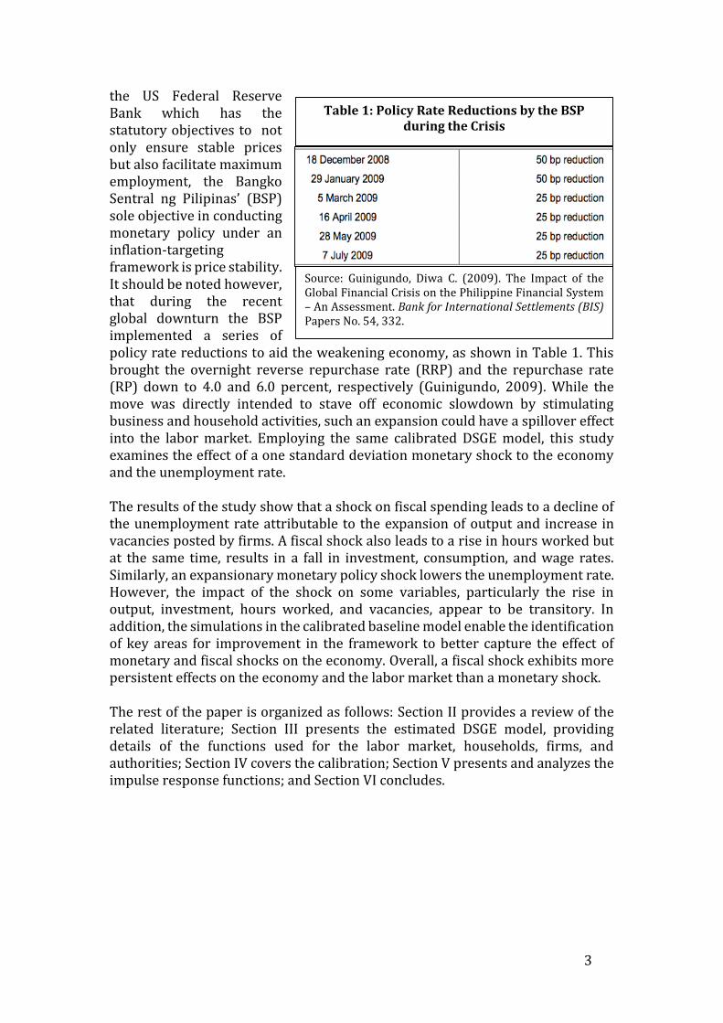
5.2 Monetary Shock Employing the same framework, this section simulates a one-period one standard deviation negative monetary policy shock to analyze the impulse responses of selected variables, especially unemployment, as shown in Figure 4. Following the expansionary shock, the households increase their hours worked resulting in output expansion, both variables peak on impact. The same is observed for consumption and investment. However, unlike the usual hump-shape response of output and investments in most literature, both variables experience a sharp decline in the next period. This pattern suggests the lack of persistence likely on

4 Brooks (2002) examines the high unemployment in the Philippines using regression and cointegration analysis and finds a parallel conclusion that unemployment rate and real GDP growth are negatively correlated.

Figure 3: Impulse Responses to a Fiscal Shock

Legend: Y is output, C is consumption, I is investment, ur is unemployment rate, h is hours worked, v is vacancy, w is wage, pii is gross inflation and R is nominal interest rate

19

account of the absence of some frictions. 5 It appears that since there are no adjustment costs on capital, investment is able to instantaneously undertake the necessary adjustment right after the shock to meet the higher future demand (Bouakez, Cardia, and Ruge-Murcia, 2002 and Christiano, Eichenbaum, and Evans, 2005).

As expected, the monetary shock lowers the nominal interest rates raising the stochastic discount factor thereby enhancing the marginal value of a worker to the firms. The firms are encouraged to post vacancies today as the expected cumulative benefit from the precluded hiring costs increases. Put in a different way, the cost of hiring now is lower than the cost of posting vacancies in the future. Hence, the expected lifetime profit for the firms rises providing the firms more incentive to post vacancies at the current period, not to mention the improvement in the marginal revenue product following the output expansion. The increase in vacancies means that more unemployed household members could get jobs,

5 Using Laplace’s method, Majuca (2011) concludes that the frictions critical to capturing the dynamics of Philippine data are investment adjustment costs, habit formation, as well as price and wage rigidities.

Figure 4: Impulse Responses to a Monetary Shock

Legend: Y is output, C is consumption, I is investment, ur is unemployment rate, h is hours worked, v is vacancy, w is wage, pii is gross inflation and R is nominal interest rate

10 20 30-2

0

2

4

6

8Y

10 20 300

0.1

0.2

0.3

0.4

0.5C

10 20 30-10

0

10

20

30I

10 20 30-5

0

5

10

15h

10 20 30-10

0

10

20

30v

10 20 30-4

-3

-2

-1

0ur

10 20 300

0.2

0.4

0.6

0.8w

10 20 30-0.5

0

0.5

1

1.5pii

10 20 30-0.1

-0.08

-0.06

-0.04

-0.02

0R

20

hence, unemployment rate falls. Following a one period lag response from the improvement in output, the unemployment rate dips the lowest in the second quarter.

The improvement in the marginal productivity and the rise in work hours translating to heightened disutility from working drive the wage rates up. However, a sharp rise could be unlikely in the Philippine setting. According to Cacnio (2012), wages in the country appear to have become relatively unreceptive to output growth because of the oversupply of labor and the wage structure of the country resulting in substantial wage stickiness. The average annual labor force growth rate from 2005 to 2013 averaged at 1.89 percent, as in Figure 5. Pitterle and Zhang (2014) characterize the country’s labor force expansion as among the fastest in East Asia. Figure 6 plots the year-on-year growth rate of real minimum wage in the National Capital Region (NCR). This hints that the model is unable to fully capture the wage condition in the country, probably due to the lack of wage friction in the framework. The overall results of the calibrated model indicate that expansionary monetary policy can potentially contribute to lowering the unemployment rate.

6 Conclusion This paper is an antecedent application of the DSGE framework that incorporates labor search theory to the Philippines to examine and analyze the impact of fiscal and monetary shocks on output and unemployment. Unemployment in the Philippines remains a challenge for policymakers as it stubbornly hovers at seven percent despite the remarkable economic performance in the recent years. Results from the calibrated baseline model show that both expansionary fiscal and monetary shocks lead to an expansion in output and an increase in vacancies, translating to a decline in the unemployment rate. Moreover, a fiscal shock leads to an increase in the hours worked but a fall in investment, consumption, and wage

Source: www.adb.org

0

2

4

6

8

10

12

2005 2006 2007 2008 2009 2010 2011 2012 2013

Figure3:Cross-CountryLaborForceExpansionRate

Indonesia Korea,Republicof Malaysia

Philippines Thailand VietNam

Figure 5: Cross-country Labor Force Expansion

Source: National Wages and Productivity Commission, Author’s calculations

-10%

0%

10%

20%

30%

40%

50%

60%

Q1Q3Q1Q3Q1Q3Q1Q3Q1Q3Q1Q3Q1Q3Q1Q3Q1Q3Q1Q3Q1Q3

2004 2005 2006 2007 2008 2009 2010 2011 2012 2013 2014

Figure7:RealMinimumWage,NationalCapitalRegion

Year-on-YearGrowthRate

Non-Agrculture Agriculture

Figure 6: Real Minimum Wage, NCR Year-on-Year Growth Rate

21

rates. On the contrary, a negative monetary shock results in a rise in consumption, investment, hours worked, and wage rates. Overall, the fiscal shock exhibits more persistent effects on the economy and the labor market compared to the monetary shock. Based on the study, a number of drawbacks in the simplified model can be identified. First, the need to incorporate more frictions to improve the overall performance of the model, specifically, habit persistence, adjustment costs of investment, and wage rigidity. This would generate more persistence in the impulse response functions, especially in the monetary shock. Second, employ actual data instead of stochastic simulation methods in generating the impulse response functions. This enhancement would provide more insights on the country’s unemployment condition. The nation’s unemployment is characterized by a structural setback stemming from the disparity between the job requirements set by businesses and the skills possessed by the available talent pool.6 Employing Bayesian estimation will determine matching efficiency of the labor market and help shed light on the structural unemployment in the country. Furthermore, since the model is primarily designed for formal sector employment, the use of actual data from the NCR instead of the whole Philippines would offer a more precise assessment (i.e., relatively more standardized unemployment opportunities). Lastly, the concurrent application of vector autoregression (VAR) analysis will better assess the fit of the impulse response functions.

Nevertheless, the present model allows us to advance our understanding of the Philippine unemployment dynamics and the effectiveness of policies in stimulating growth and addressing the unemployment in the country. It paves the way for the exploration of related research on the area. Moreover, in light of the findings of this paper on the positive impact of an expansionary monetary policy shock on unemployment, the Central Bank could undertake further empirical studies on how its policies affect labor market conditions. The Central Bank may find reason to reassess its conduct of monetary policy towards pursuing a more active policy stance on supporting the general government in addressing the country’s unemployment condition. 7,8

5 The identified contributing factors include: 1) the cultural mindset of parents on particular professions, regardless of whether there is a demand for it in the economy; (2) the passing trends of in demand professions; (3) the misperception of what is in demand coupled with herd mentality among the market agents; and (4) the schools basing their course offerings on what they believe the parents/students are keen on, thereby reinforcing the possibly misplaced expectations. (Lorenciana, 2014, Habito, 2013, and Orillaza, 2014) 7 Lim (2006) similarly raises the issue of a more employment-sensitive monetary policy to help ease labor market conditions. Among the components of an alternative monetary policy that he recommends is the inclusion output and employment goals as part of the objectives of monetary policy, citing the US Fed’s monetary policy approach wherein the Fed adjusts its policy rates to veering the economy to the direction it wants taking into account its multiple objectives. 8 Cacnio (2012) surmises that there is flattening of the Phillips curve in the country in the recent decade. This implies that policy changes geared towards ameliorating unemployment will not translate to substantial upward pressure on inflation.

22

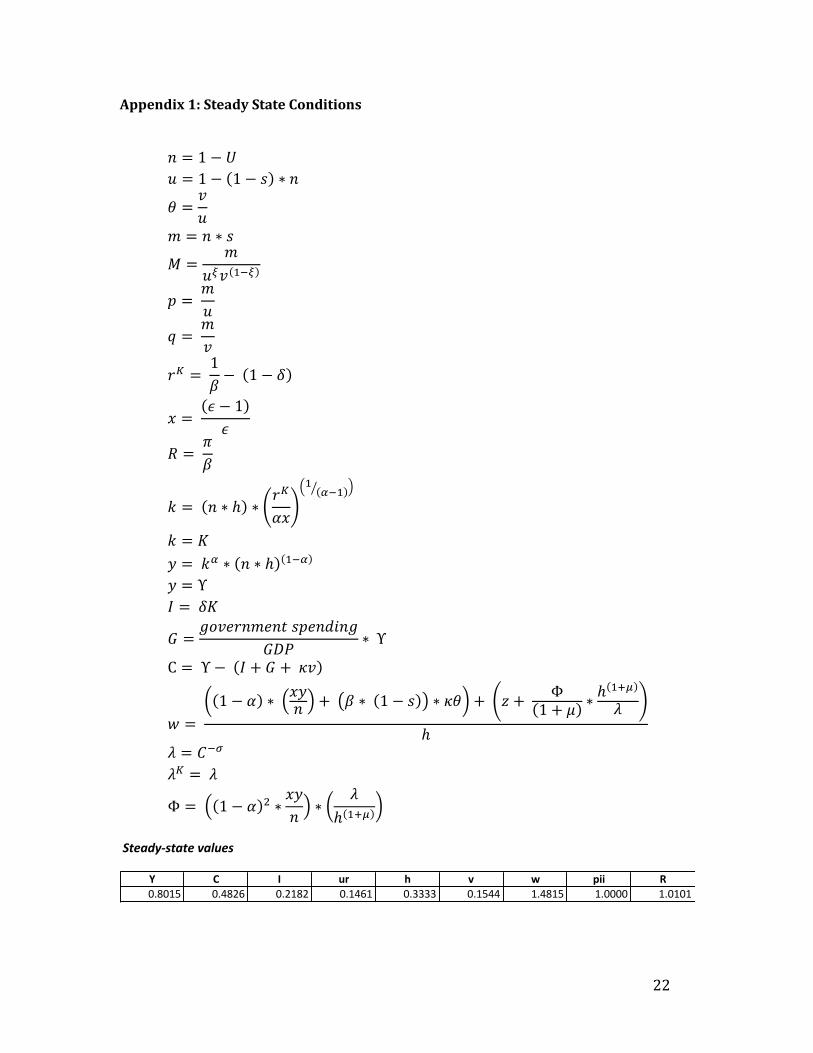
Appendix 1: Steady State Conditions

𝑛 = 1 − 𝑈

𝑢 = 1 − (1 − 𝑠) ∗ 𝑛

휃 =𝑣

𝑢

𝑚 = 𝑛 ∗ 𝑠

𝑀 =𝑚

𝑢𝜉𝑣(1−𝜉)

𝑝 = 𝑚

𝑢

𝑞 = 𝑚

𝑣

𝑟𝐾 = 1

𝛽− (1 − 𝛿)

𝑥 = (𝜖 − 1)

𝜖

𝑅 = 𝜋

𝛽

𝑘 = (𝑛 ∗ ℎ) ∗ (𝑟𝐾

𝛼𝑥)

(1(𝛼−1)⁄ )

𝑘 = 𝐾

𝑦 = 𝑘𝛼 ∗ (𝑛 ∗ ℎ)(1−𝛼)

𝑦 = Υ

𝐼 = 𝛿𝐾

𝐺 =𝑔𝑜𝑣𝑒𝑟𝑛𝑚𝑒𝑛𝑡 𝑠𝑝𝑒𝑛𝑑𝑖𝑛𝑔

𝐺𝐷𝑃∗ Υ

C = Υ − (𝐼 + 𝐺 + 휅𝑣)

𝑤 =

((1 − 𝛼) ∗ (𝑥𝑦𝑛 ) + (𝛽 ∗ (1 − 𝑠)) ∗ 휅휃) + (𝑧 +

Φ(1 + 휇)

∗ℎ(1+𝜇)

휆)

ℎ

휆 = 𝐶−𝜎

휆𝐾 = 휆

Φ = ((1 − 𝛼)2 ∗𝑥𝑦

𝑛) ∗ (

휆

ℎ(1+𝜇))

Steady-statevalues

Y C I ur h v w pii R

0.8015 0.4826 0.2182 0.1461 0.3333 0.1544 1.4815 1.0000 1.0101

23

Appendix 2: Log-linear Equilibrium Conditions

Labor Market

��𝑡 = (1 − 𝑠)��𝑡−1 + 𝑚

𝑛��𝑡

𝑈 ��𝑡 + 𝑛 ��𝑡 = 0 ��𝑡 = ��𝑡 + 𝜉��𝑡 + (1 − 𝜉) ��𝑡

𝑢 ��𝑡 = (𝑠 − 1) 𝑛 ��𝑡−1 휃𝑡 = 𝑣𝑡 + ��𝑡 ��𝑡 = ��𝑡 − 𝑣𝑡 ��𝑡 = ��𝑡 − ��𝑡

Households

휆𝑡 = 𝛾𝑡 − 𝜎 ��𝑡

��𝑡 = (1 − 𝛿) ��𝑡−1 + 𝐼

𝐾 (𝐼𝑡 + ��𝑡)

휆𝑡 = 휆𝑡𝐾 + ��𝑡

휆𝑡 = 휆𝑡+1 + ��𝑡+1 − ��𝑡+1

휆𝑡𝐾 = 𝛽𝑟𝐾(휆𝑡+1 + ��𝑡+1

𝐾 ) + 𝛽(1 − 𝛿)휆𝑡+1𝐾

Intermediate Goods Firms

��𝑡 = ��𝑡 + 𝛼��𝑡 + (1 − 𝛼)��𝑡 ℎ𝑡

��𝑡𝐾 = ��𝑡 + ��𝑡 − ��𝑡

−휅

𝑞 ��𝑡 = (1 − 𝛼)

𝑥𝑦

𝑛(��𝑡 + ��𝑡 − ��𝑡) + 𝑤ℎ (��𝑡 + ℎ𝑡) +

𝛽 (1 − 𝑠)𝜅

𝑞 (휆𝑡+1 − 휆𝑡

+ ��𝑡+1)

Retailers

24

��𝑡 = 𝜄

(1+ 𝛽𝜄)��𝑡−1 +

𝛽

(1+ 𝛽𝜄)��𝑡+1 +

(1−𝛽𝜑)(1−𝜑)

𝜑(1+ 𝛽𝜄)��𝑡 + 𝜖��

Wages and Hours Bargaining

𝑤ℎ (��𝑡 + ℎ𝑡) = 휂 [(1 − 𝛼)

𝑥𝑦

𝑛(��𝑡 + ��𝑡 − ��𝑡) + 𝛽(1 − 𝑠)휅휃

(휆𝑡+1 − 휆𝑡 + 휃𝑡+1)

]

+ (1 − 휂 )Φ𝜒

1 + 휇

ℎ(1+𝜇)

휆 [��𝑡 + (1 + 휇)ℎ𝑡 − 휆𝑡

]

��𝑡 + ��𝑡 − ��𝑡 − ℎ𝑡 = ��𝑡 + 휇 ℎ𝑡 − 휆𝑡

Monetary Policy

��𝑡 = 𝜌𝑅��𝑡−1 + (1 − 𝜌𝑅) (𝜙𝜋��𝑡 + 𝜙ΥΥ𝑡) − 휁𝑚𝑝,𝑡

Closing the Model ��𝑡 = Υ𝑡

��𝑡 = K𝑡

ΥΥ𝑡 = 𝐶��𝑡 + 𝐼𝐼𝑡 + 𝐺��𝑡 + 휅𝑣𝑣𝑡

Shocks

휁𝑚𝑝,𝑡 = 휀��,𝑡

��𝑡 = 𝜌𝐺��𝑡−1 + 휀��,𝑡

25

References 1. Adjemian, Stéphane, Bastani, Houtan, Karamé, Frédéric, Juillard, Michel, Maih,

Junior, Mihoubi, Ferhat, Perendia, George, Pfeifer, Johannes, Ratto, Marco, and Villemot, Sébastien (2011). Dynare Reference Manual, version 4. Dynare Working Papers 1, CEPREMAP. Accessed on 6 February 2015 at http://www.dynare.org/wp-repo/dynarewp001.pdf

2. Albert, Jose Ramon G. (August 2014). Is Growth Really Jobless? Philippine Institute for Development Studies (PIDS), Policy Notes No. 2014-16. Accessed on 28 March 2015 at http://dirp4.pids.gov.ph/webportal/CDN/PUBLICATIONS/pidspn1416.pdf

3. Alegado, Siegfrid O. (24 January 2014). PHL unemployment: A Problem Runs Deep. GMA News. Accessed 20 April 2015, at http://www.gmanetwork.com/news/story/345344/economy/business/phl-unemployment-a-problem-runs-deep

4. Bouakez, Hafedh, Cardia, Emanuela, and Ruge-Murcia, Francisco J. (2002). Habit Formation and the Persistence of Monetary Shocks. Bank of Canada, Working Paper 2002-27. Accessed on 29 April 2015 at http://www.bankofcanada.ca/2002/10/working-paper-2002-27/

5. Boz, Emine, Durdu, Bora, and Li, Nan (October, 2012). Emerging Market Business Cycles: The Role of Labor Market Frictions. International Monetary Fund (IMF) Working Paper 12/237. Accessed on 26 April 2015 at https://www.imf.org/external/pubs/ft/wp/2012/wp12237.pdf

6. Brooks, Ray (February 2002). Why Unemployment is High in the Philippines? International Monetary Fund (IMF). IMF Working Paper 02/23. Accessed on 16 March 2015 at http://www.imf.org/external/pubs/ft/wp/2002/wp0223.pdf

7. Bu, Yisheng (2006). Fixed Capital Stock Depreciation in Developing Countries: Some Evidence From Firm Level Data. Journal of Development Studies, 42(5), 881-901. Accessed on 8 May 2015 at https://ideas.repec.org/a/taf/jdevst/v42y2006i5p881-901.html

8. Cacnio, Faith Christian Q. (Mar-Apr 2012). Inflation Dynamics and Unemployment Rate in the Philippines. Bangko Sentral ng Pilipinas (BSP) Economic Newsletter No. 12-02. Accessed 29 March 2015 at http://www.bsp.gov.ph/downloads/EcoNews/EN12-02.pdf.

9. Calvo, Guillermo A. (September 1983). Staggered Prices in a Utility-Maximizing Framework. Journal of Monetary Economics 12, 383-98. Accessed on 18 April 2015 at http://isites.harvard.edu/fs/docs/icb.topic500592.files/calvo.pdf

10. Chandran, Rina and Chen, Sharon (30 January 2015), “Move Over Thailand, the Philippines is Southeast Asia's Strong Man,” Bloomberg News. Accessed on 16 April 2015 at http://www.bloomberg.com/news/articles/2015-01-30/move-over-thailand-the-philippines-is-southeast-asia-s-strong-man

11. Christiano, Lawrence J., Eichenbaum, Martin, and Evans, Charles L. (2005). Nominal Rigidities and the Dynamic Effects of a Shock to Monetary Policy. Journal of Political Economy, 113(1). Accessed 1 May 2015 at https://ideas.repec.org/a/ucp/jpolec/v113y2005i1p1-45.html

26

12. Christiano, Lawrence, Trabarndt, Mathias, and Walentin, Karl (June 2010), “DSGE Models for Monetary Policy Analysis,” National Bureau of Economic Research (NBER), Working Paper No. 16074. Accessed 15 April 2015 at http://www.nber.org/papers/w16074

13. Dacuycuy, Lawrence and Majuca, Ruperto (14 November 2014). An Open-Economy DSGE Model with Nontradables and Remittances. Presentation during the Philippine Economic Society (PES), 52nd Annual Meeting, Intercontinental Hotel, Makati. Accessed on 28 April 2015 at https://phileconsoc.files.wordpress.com/.../dsge-majuca_dacuycuy.pptx

14. Doppelhofer, Gernot (May 2009). Intertemporal Macroeconomics. Cambridge Essays in Applied Economics, Cambridge UP. Accessed on 1 May 2015 at https://www.nhh.no/Files/Filer/institutter/sam/cv/papers/Intertemporal_Macroeconomics.pdf

15. Doraisami, Anita (June 2011). The Global Financial Crisis: Countercyclical Fiscal Policy Issues and Challenges in Malaysia, Indonesia, the Philippines, and Singapore. Asian Development Bank Institute (ADBI) Working Paper Series No. 288. Accessed 9 May 2015 at http://www.adbi.org/files/2011.06.07.wp288.gfc.countercyclical.fiscal.policy.issues.challenges.pdf

16. Epstein, Brendan and Shapiro, Alan Finkelstein (August, 2014). Employment and Firm Heterogeneity, Capital Allocation, and Countercyclical Labor Market Policies. Board of Governors of the Federal Reserve System, International Finance Discussion Papers No. 1115. . Accessed on 27 April 2015 at www.federalreserve.gov/pubs/ifdp/2014/1115/ifdp1115.pdf

17. Faccini, Renato, Millard, Stephen, and Zanetti, Francesco (February 2011). Wage Rigidities in an Estimated DSGE Model of the UK Labour Market. Bank of England Working Paper No. 408. Accessed on 18 February 2015 at http://papers.ssrn.com/sol3/papers.cfm?abstract_id=1765841

18. Galí, Jordi (April 2010). Monetary Policy and Unemployment. National Bureau Of Economic Research (NBER) Working Paper Series, Working Paper 15871. Accessed on 20 April 2015 at http://www.nber.org/papers/w15871

19. Gertler, Mark, Sala, Luca, and Trigari, Antonella (December 2008). An Estimated Monetary DSGE Model with Unemployment and Staggered Nominal Wage Bargaining. Journal of Money, Credit and Banking, 40(8), 1713-1764. Accessed on 16 April 2015 https://ideas.repec.org/a/mcb/jmoncb/v40y2008i8p1713-1764.html

20. Griffoli, Tommaso Mancini (2007). Dynare User Guide: An Introduction to the Solution & Estimation of DSGE Models. Unpublished Manuscript. Accessed on 6 February 2015 at http://www.dynare.org/documentation-and-support/user-guide/Dynare-UserGuide-WebBeta.pdf

21. Guillaume, Rocheteau (2006). Understanding Unemployment. Federal Reserve Bank of Cleveland. As cited in Thoma, Mark (October 2006). The Search-Matching Theory of Unemployment. Economist’s View. Accessed on 28 April 2015 http://economistsview.typepad.com/economistsview/2006/10/the_searchmatch.html

27

22. Guinigundo, Diwa C. (2009). The Impact of the Global Financial Crisis on the Philippine Financial System – An Assessment. Bank for International Settlements (BIS) Papers No. 54, 317-342. Accessed on 9 May 2015 at http://www.bis.org/publ/bppdf/bispap54s.pdf

23. Habito, Cielito F. (5 August 2013). Addressing the Jobs Mismatch. No Free Lunch Column, Philippine Daily Inquirer. Accessed 29 April 2015 at http://opinion.inquirer.net/58177/addressing-the-jobs-mismatch

24. Jawan, Sarwar, Mahmud, Ahmed Saber, and Papageorgiou, Chris (September 2014). What Is Keynesian Economics? Finance and Development, 51(3). Accessed 10 April 2015 at http://www.imf.org/external/pubs/ft/fandd/2014/09/basics.htm

25. Kato, Ryuta Ray and Miyamoto, Hiroaki (November 2012). Fiscal Stimulus and Labor Market Dynamics in Japan. Economics & Management Series, 2012-19. Accessed 14 March 2015 at http://nirr.lib.niigata-u.ac.jp/bitstream/10623/38299/1/EMS_2012_19.pdf

26. Kritz, Ben D. (3 September 2014). Redefining ‘jobless growth’. The Manila Times. Accessed 4 April 2015 at http://www.manilatimes.net/redefining-jobless-growth/123860/

27. Kuo, Chun-Hung and Miyamoto, Hiroaki (forthcoming). An Estimated DSGE Model with Fiscal Policy and Unemployment.

28. Kuo Chun-Hung and Miyamoto, Hiroaki (2015). Fiscal Stimuli in the Form of Job Creation Subsidies. Elsevier Inc. Journal of Macroeconomics 43. Accessed on 26 April 2015 at https://ideas.repec.org/p/iuj/wpaper/ems_2014_06.html

29. Lim, Joseph (September 2006). Philippine Monetary Policy: A Critical Assessment and Search for Alternatives. Political Economy and Research. University of Massachusetts Amherst. Accessed on 4 May 2015 at http://www.peri.umass.edu/fileadmin/pdf/inflation/lim_paper10.pdf

30. Lorenciana, Carlo S. (12 August 2014). Jobs Mismatch Keeps Unemployment High. The Freeman, The Philippine Star. Accessed 29 April 2015 at http://www.philstar.com/cebu-business/2014/08/12/1356737/jobs-mismatch-keeps-unemployment-high

31. Majuca, Ruperto P. (March 2011). An Estimated (Closed Economy) Dynamic Stochastic General Equilibrium Model for the Philippines: Are There Credibility Gains from Committing to an Inflation Targeting Rule?. Philippine Institute for Development Studies, Discussion Paper Series No. 2011-04. Accessed on 26 April 2015 at http://serp-p.pids.gov.ph/details.php?pid=4924&param=Majuca%2C+Ruperto+P.

32. Mandelman, Federico S. and Zanetti, Francesco (October 2008). Estimating General Equilibrium Models: An Application with Labour Market Frictions. Bank of England, Centre for Central Banking Studies Technical Handbook No. 1. Accessed on 10 February 2015 at http://www.bankofengland.co.uk/education/Pages/ccbs/technical_handbooks/techbook1.aspx

33. Mankiw, N. Gregory (2010). Macroeconomics, 7th Edition. Worth Publishers. 34. Mayer, Eric, Moyen, Stéphane, and Stähler, Nikolai (2010). Government

Expenditures and Unemployment: A DSGE Perspective. Deutsche Bundesbank,

28

Discussion Paper Series 1: Economic Studies No 18/2010. Accessed on 1 May 2015 at https://ideas.repec.org/p/zbw/bubdp1/201018.html

35. McNelis, Paul D., Glindro, Eloisa T., Co, Ferdinand S., and Dakila, Francisco G. Jr. (2009). Macroeconomic Model for Policy Analysis and Insight (A Dynamic Stochastic General Equilibrium Model for the Bangko Sentral ng Pilipinas). Bangko Sentral ng Pilipinas (BSP) Working Paper Series 2009-01. Accessed 20 February 2015 at www.bsp.gov.ph/downloads/publications/2009/wps200901.pdf

36. McNelis, Paul D. and Staff of the Center for Monetary and Financial Policy, BSP. A Bayesian DSGE Prototype for BSP. Technical Report, USAID. Accessed 20 February 2015 at http://pdf.usaid.gov/pdf_docs/Pnadj582.pdf

37. Merz, Monika (1995). Search in the Labor Market and the Real Business Cycle. Journal of Monetary Economics 36, 269-300. Accessed on 18 April 2015 at https://ideas.repec.org/a/eee/moneco/v36y1995i2p269-300.html Mutschler, Willi (2014). DSGE Methods: Calibration of DSGE Models. Institute of Econometrics and Economic Statistics University of Munster. Accessed on 28 April 2015 at http://www.wiwi.uni-muenster.de/05/download/studium/dsgemodels/ss2014/slide_12.pdf

38. Monacelli, Tommaso, Perotti, Roberto, and Trigari, Antonella (2010). Unemployment Fiscal Multipliers. Journal of Monetary Economics, 57(5), 531–553. Accessed on 8 May 2015 at http://www.rperotti.com/doc/MonacelliPerottiTrigariJME2010.pdf

39. Mortensen, Dale T. and Pissarides, Christopher A. (July 1994). Job Creation and Job Destruction in the Theory of Unemployment. Review of Economic Studies 61(3), 397-415. Accessed on 8 May 2015 at http://www.iab.de/UserFiles/File/downloads/gradab/Dokumente%20Garloff/Mortensen_Pissarides_1994_Job%20creation%20and%20job%20destruction%20in%20the%20theory%20of%20unemployment_RES_pp_397_415.pdf

40. Orillaza, Jennifer M. (1 May 2014). Labor Mismatch, or What Ails the PHL Jobs Market. GMA News. Accessed 29 April 2015 at http://www.gmanetwork.com/news/story/359201/economy/companies/labor-mismatch-or-what-ails-the-phl-jobs-market

41. Philipp Engler (November 2011). Monetary Policy and Unemployment in Open Economies. National Centre of Econometric Research (NCER) Working Paper Series, Working Paper No. 77. Accessed 30 April 2015 at http://www.ncer.edu.au/papers/documents/WPNo77.pdf

42. Pissarides, Christopher A. (2000). Equilibrium Unemployment Theory, Second Edition. MIT Press, Cambridge, MA.

43. Pitterle, Ingo and Zhang, Rui (19 March 2014). The Philippines: A Case of Jobless Growth. World Economic Situation and Prospects, Weekly Highlight, World Bank. Accessed on 17 April 2015 at http://www.un.org/en/development/desa/policy/wesp/wesp_wh/wesp_wh49.pdf

44. Smets, Frank and Wouters, Raf (August 2002). An Estimated Dynamic Stochastic General Equilibrium Model of the Euro Area. European Central Bank

29

(ECB), ECB Working Paper Series, Working Paper No. 171. Accessed on 5 February 2015 at https://www.ecb.europa.eu/pub/pdf/scpwps/ecbwp171.pdf

45. Tang, Hsiao Chink, Liu, Philip, and Cheung, Eddie C. (December 2010). Changing Impact of Fiscal Policy on Selected ASEAN Countries. Asian Development Bank (ADB) Working Paper Series on Regional Economic Integration No. 70. Accessed on 9 May 2015 at http://www.adb.org/publications/changing-impact-fiscal-policy-selected-asean-countries

46. Thomas, Carlos (2008). Search and Matching Frictions and Optimal Monetary Policy. Journal of Monetary Economics, 55, 936-56. Accessed on 8 May 2015 at https://ideas.repec.org/a/eee/moneco/v55y2008i5p936-956.html

47. Tovar, Camilo E. (September 2008). DSGE Models and Central Banks. Bank for International Settlements, Working Papers No 258. Accessed on 25 April 2015 at http://www.bis.org/publ/work258.htm

48. Walsh, Carl E. (2003). Labor Market Search and Monetary Shocks. Elements of Dynamic Macroeconomic Analysis, 451-486. Accessed on 25 March 2015 at http://people.ucsc.edu/~walshc/MyPapers/DynamicMacroVol_chapter_p451-486.pdf

49. Ubac, Michael Lim (12 February 2014). Aquino on rise in joblessness: What went Wrong? Philippine Daily Inquirer. Accessed 4 April 2015 at http://newsinfo.inquirer.net/577058/aquino-on-rise-in-joblessness-what-went-wrong