A drifting impact oscillator with periodic impulsive loading: Application topercussive drilling

A. Depouhona,b, V. Denoela, E. Detournayb,c,∗

aStructural Engineering, ArGEnCo, Department of Applied Sciences, Universite de Liege, BelgiumbDepartment of Civil Engineering, University of Minnesota, MN, USA

cCSIRO Earth Science and Resource Engineering, Australia

Abstract

Percussive drilling is extensively used to drill hard rocks in the earth resource industry, where it performs best compared

to other drilling technologies. In this paper, we propose a novel model of the process that consists of a drifting oscillator

under impulsive loading coupled with a bilinear force/penetration interface law, together with a kinetic energy threshold

for continuous bit penetration. Following the formulation of the model, we analyze its steady-state response and show

that there exists a parallel between theoretical and experimental predictions, as both exhibit a maximum of the average

penetration rate with respect to the vertical load on bit. In addition, existence of complex long-term dynamics with the

coexistence of periodic solutions in certain parameter ranges is demonstrated.

Keywords: Percussive drilling, Periodic orbit, Drifting oscillator, Impact system, Piecewise-linear system, Hybrid

system

1. Introduction

Many industrial processes rely on the impulsive loading

of a first body in contact with a second one to achieve the

penetration of the former in the latter. Among these, we

find nail hammering [1, 2] or pile driving [3–5]. Another

such process is down-the-hole percussive drilling, where

penetration is achieved by repeated application of a large

impulsive force to a rock drill bit [6–8]. The impulsive force

is generated by the impact of a pneumatically-operated

piston (hammer) on a shank adapter (anvil). The kinetic

energy conveyed by the piston is transformed into com-

pressive stress waves upon contact with the adapter, waves

that propagate through the drill bit down to the rock,

leading to rock destruction by indentation, crushing and

chipping [9].

∗Corresponding author at: Department of Civil Engineering, Uni-

versity of Minnesota, MN, USA.

Email address: detou001@umn.edu (E. Detournay)

Several authors have addressed the issue of modeling

this process and have contributed to various aspects of the

problem. Two foci of interest can be identified in the lit-

erature: (i) the bit/rock interaction, i.e. the interface law

that captures the force/penetration behavior, and (ii) the

bit dynamics, that is, the prediction of bit motion under

specific loading and interface conditions. While the for-

mer topic has been addressed experimentally [10–13] and

numerically based on a continuum approach [14, 15] or

a discrete one [16], the study of bit dynamics has led to

design considerations to maximize the process efficiency

[9, 17], the development of numerical algorithms to simu-

late the process [7, 18], as well as the representation of the

process as a drifting oscillator [19–21].

The phenomena taking place at the bit/rock interface

are of very complex nature as several failure mechanisms

result from the dynamic indentation of rock in the pres-

ence of debris remaining from former impacts. While some

Preprint submitted to Physica D March 10, 2013

2

authors have proposed physics-based arguments to the de-

velopment of interaction laws, based notably on the cavity

expansion model [22], scaling arguments [23] or numeri-

cal evidence [14, 16], percussion drilling experiments have

highlighted two common trends: (i) the force/penetration

law consists of two successive phases, one associated with

the loading and the other with the unloading of the inter-

face [9, 11, 13, 24], and (ii) this law is rate-independent,

i.e. it does not depend on the penetration velocity of the

indenter [10, 24]. Furthermore, the idealization of this law

by a history-dependent bilinear model, i.e. a linear spring

with larger unloading stiffness than loading one, has been

shown to capture the essential response observed in single

impact indentation experiments as confirmed by measure-

ments [13] and by the matching of numerical results to

experimental ones in the analysis of stress waves traveling

in drill steels [25].

Percussive drilling systems are known to exhibit an op-

timal functioning configuration, in the sense that a proper

choice of the control parameters maximizes the bit aver-

age rate of penetration in the rock medium, as was evi-

denced from field measurements by [26] and conceptually

presented in [27]. Works on bit dynamics have recovered

this trend by modeling the drill bit as a drifting impact

oscillator. In these models, a superposition of harmonic

and static loadings was considered, at first, in combination

with unilateral viscoelastic or perfectly rigid contact mod-

els serially connected to a constant-force threshold slider

[19–21, 28] and, more recently, in combination with an in-

terface law based on the elasto-plastic response of a rigid

indenter in a semi-infinite medium [29]. Due to the unilat-

eral nature of the contact, these models are non-smooth

dynamical systems and belong to the class of piecewise-

smooth systems; see the monograph by di Bernardo et al.

[30] as well as the works by Leine et al. [31, 32] for an

introduction to this category of systems.

In this paper, we introduce a model for the bit dynam-

ics that also belongs to the family of drifting oscillators

but differs in two key aspects from those proposed in [19–

21, 28]. First, we consider the variable load on bit to be

periodic impulsive rather than harmonic, a specificity that

we presume more appropriate to model the activation re-

lated to repeated hammer blows. Second, we model the

force/penetration behavior at the bit/rock interface by a

modified bilinear law, partly tying up with the proposi-

tion of Ajibose [24, 29] to model the bit/rock interaction

using power laws for the loading and unloading phases. A

particularity of this second element is the introduction in

the bit/rock interaction law of a kinetic energy barrier to

dissociate static loadings from dynamic ones.

As we detail next, the model is deliberately kept as sim-

ple as possible in order to highlight the richness brought by

these two features. Given the impulsive nature of the load-

ing, the evolution of bit motion is ruled by continuous and

discrete dynamics. As such, the proposed model belongs

to the class of hybrid systems [30] that comprises, among

others, models with impacting bodies, e.g. vibro-impact

oscillators [33] or particle avalanche models [34].

Section 2 is the object of a detailed description of the

model, with the introduction of its building blocks and

governing equations. In Section 3, we present the results

of the model analysis; in particular, we focus on its steady-

state and long-term response. The paper then concludes

with a discussion of the results in Section 4.

2. Mathematical modeling

The model is a 1 degree-of-freedom drifting oscillator

subject to a combination of periodic impulsive and static

loadings with a bilinear interface law coupled to a ki-

netic energy barrier describing the force/penetration char-

acteristics. This formulation relies on several assumptions:

(i) the existence of a timescale separation between the per-

cussive activation on the one hand, and the bit motion as

well as the bit/rock interaction on the other hand, allowing

us to ignore wave propagation in the modeling of percus-

sive drilling; (ii) the modeling of the bit/rock interaction

2.2 Bit/rock interaction law 3

by a bilinear law that is essentially rate-independent, ex-

cept for the existence of a kinetic energy threshold for the

bit penetration; (iii) the reduction of the bit dynamics to

the axial motion; and (iv) the neglect of debris cleaning.

Despite these strong simplifying assumptions, this model

captures the essence of the process response, and we be-

lieve it could be a proper springboard for the development

of future more refined models of the process.

Figure 1: Free body diagram of the drill bit.

2.1. Governing equations

The bit free body diagram is shown in Figure 1. We

denote the oscillator mass by M . Its vertical displacement

y is positively defined in the downward direction. We refer

to the static force and impulsive loading by FS and δFT ,

while the bit/rock interaction force is named FR. The

action of gravity is considered. The equation governing

the bit dynamics is obtained by application of Newton’s

law

My = Mg + FS + δFT − FR. (1)

The impulsive loading δFT , resulting from the percus-

sive activation, chosen to be of period T and of constant

impulse I at each pulse, reads

δFT (t) = I∑i∈N

δ (t− iT − ts) , (2)

with δ (·) Dirac’s delta function and 0 ≤ ts < T an arbi-

trary time shift. It is thus zero everywhere but at specific

time instants spaced by a duration T , at which it increases

the momentum of the bit. The equation of motion thus

reduces to

My = Mg + FS − FR, (3)

Figure 2: Bilinear bit/rock interaction law.

everywhere but at the instants of impact, ti = iT + ts, at

which the bit velocity experiences an instantaneous jump

y(t+i ) = y(t−i ) +ηI

M, i ∈ N, (4)

where 0 ≤ η ≤ 1 is an efficiency coefficient that accounts

for the momentum transfer to the rock if the bit is in con-

tact with the rock at the time of impact. This momen-

tum transfer, which involves generation and propagation

of waves in the rock medium, is assumed to take place

instantaneously when viewed at the timescale of the bit

motion; it can therefore be embodied in the coefficient η.

For this preliminary study, however, we assume that η = 1,

whether the bit is contacting the rock or not at the moment

of application of the impulsive load. This approximation is

in accordance with numerical simulations indicating that

the maximum amount of dissipated energy is at most 5% of

the impact energy of the piston when the bit is in contact

with the rock [35].

2.2. Bit/rock interaction law

The rate-independent bilinear bit/rock interaction law,

which relates the force on bit, FR, to the penetration while

drilling, p, follows from single impact dynamic indentation

experiments. This law depends on two parameters: the

loading stiffness KR and the unloading one γKR > KR.

Figure 2 illustrates this relation and indicates along the

drilling cycle three non-smooth locations with respect to

the interaction law: the points of lower, peak and upper

penetration. While penetration and bit position are equiv-

alent in the frame of single impact experiments, this is no

longer the case when considering repeated impacts. To

2.2 Bit/rock interaction law 4

A

B

C+ = C-

E

D FA D

C-C+

BE

F

12

Figure 3: Bit/rock interaction model with force as a function of the

bit penetration (left) and bit displacement (right).

relate the force on bit to the bit position, we define the

penetration while drilling during the nth drilling cycle as

the advance of the bit with respect to the final contact po-

sition of the bit/rock interface during the previous drilling

cycle plus the residual penetration, has the cycle not been

completed

p(n) (t) = y (t)− y(n)` +F

(n)R,`

KR. (5)

Specific to this definition is the introduction of the his-

tory variables y(n)` and F

(n)R,` . These are defined as the bit

position and the force on bit at the beginning of the nth

drilling cycle, the lower point of this cycle, hence index `.

Correspondences with the peak and upper drilling cycle

locations, (y(n)p , FR,p) and (y

(n)u , FR,u), can also be estab-

lished when representing the bit/rock interaction law in

the (y, FR)-space. Figure 3 illustrates this match for two

consecutive drilling cycles. Points A, C and F define the

lower characteristics of drilling cycles while B and E are

located at their peaks. The upper locations are denoted

by D and F.

It is important to note that history variables do depend

on the past trajectory of the system in a discrete manner.

They capture the state of the bit/rock interaction law at

a specific instant and, as such, evolve in a stepwise man-

ner. Their update takes place at the instant the system

goes through the corresponding non-smooth point of the

interface law.

Following the definition of the penetration while drilling

and those of the history variables, the bit/rock interaction

law, in terms of the axial position, reads

F(n)R (y) =

F

(n)R,` +KR

[y (t)− y(n)`

]if loading,

F(n)R,p + γKR

[y (t)− y(n)p

]if unloading,

0 if no contact.

(6)

While experimental results do support the assumption of

rate-independence embedded in the above interaction law,

this independence must nonetheless be bounded above and

below. The upper bound reflects the limit at which the

indentation velocity cannot be neglected compared to the

wave speed in the rock medium. The lower bound needs

to be considered to account for cases when the bit is close

to be at rest, to differentiate static and dynamic loadings.

The upper bound is, in practice, never encountered but the

lower one is and requires an adjustment of the interaction

law. In that perspective, we complement the bilinear law

with an energy barrier; that is, a new drilling cycle can

only start provided the bit kinetic energy is larger than a

given energy threshold Ek`

1

2My2` ≥ Ek` . (7)

This barrier dissociates the static indentation of rock from

the dynamic one and is instantaneous at the timescale of

bit motion. It implies that continuous penetration, i.e.

over more than one drilling cycle, can only take place if

the bit kinetic energy is larger than a threshold. This

barrier leads to a direct loss of kinetic energy of the bit

when a new drilling cycle is started. Equations (6) are

thus complemented by the velocity update

y+` =

√y−`

2 − 2Ek

`

M if y−` ≥√

2Ek` /M,

0 otherwise,

(8)

which drives the bit to a standstill should its kinetic energy

be below the barrier. The symbols y−` and y+` refer to the

velocities just before and after the beginning of the drilling

cycle.

2.4 Dimensionless formulation 5

2.3. Drilling Phases

The conditional, in fact sequential, nature of the con-

tact model conducts us to define four drilling phases.

(i) Forward Contact (FC): the bit motion is downwards

while there is contact between the bit and the rock.

(ii) Backward Contact (BC): contact is established but

the bit is moving upwards.

(iii) Free Flight (FF): the bit is flying off the hole bottom;

the force exerted by the rock is zero.

(iv) Standstill (SS): the bit is at rest and in contact with

the rock; the reaction force from the rock exactly

compensates the vertical force on the bit.

With each regime, we then associate a specific expression

of the equation of motion that we write in terms of the pen-

etration while drilling rather than the bit position, given

that p(t) = y(t). Dropping the drilling cycle number for

legibility, they read

FC : Mp+KRp = Mg + FS ,

BC : Mp+ γKRp = Mg + FS + (γ − 1)KRpp,

FF : Mp = Mg + FS ,

SS : p = p = 0.

(9)

They are completed by the velocity jump conditions of

equations (4) and (8) where we set y(t) = p(t) and η = 1.

It is worth mentioning that our choice of representing the

bit motion by the penetration while drilling rather than

the position aims at preventing the drift of the system in

the phase plane and ensures the boundedness of the state-

space when studying the motion of the bit.

To complete the definition of the system dynamics, we

introduce the conditions that govern the transition from

one drilling phase to the other. Ten cases have to be con-

sidered. References to points in Figure 3 are made to illus-

trate their occurrence on the force/displacement response

curve of the interface model.

• FC → BC: The drilling cycle reaches its peak, i.e.

the bit velocity becomes zero, p = 0; see points B

and E.

• BC → FF: The drilling cycle completes at its upper

point, i.e. the force on bit vanishes, p = pp (γ−1)/γ;

point F represents this transition.

• FF → FC: A new drilling cycle begins, i.e. the bit

reconnects with the hole bottom after a period of

free flight, p = pu, and has sufficient energy p` ≥√2Ek` /M . This occurs at point F, where the pene-

tration is reset to zero at the beginning of the next

drilling cycle, p` = 0.

• BC → ∆θ′i → FC: A new drilling cycle begins due

to the percussive activation, i.e. the bit velocity

changes sign before the current drilling cycle has

completed, p+i · p−i < 0, and the activation increases

the bit energy above the barrier; with this transi-

tion, a residual penetration exists at the beginning

of the next drilling cycle, and (p`, FR,`) > 0. This

corresponds to point C.

In case the energy of the bit is insufficient at the beginning

of a drilling cycle, i.e. at a transition to forward contact,

the bit motion is switched to standstill, in accordance with

equation (8), and remains in that phase until the next

activation takes place. Three transitions are thus possible:

FF→ SS, BC→ SS and SS→ ∆θ′i → FC. The transitions

due to activation that do not lead to a change of drilling

phase then complete the list: FC → ∆θ′i → FC, BC →

∆θ′i → BC and FF→ ∆θ′i → FF.

2.4. Dimensionless formulation

For the ensuing analysis, it is convenient to reformulate

the governing equations in dimensionless form. Choosing

the timescale proportional to the resonant period of the

spring/mass system associated with the bit/rock interface

at loading, and the reference length scale as the peak pen-

etration engendered by the only action of an activation on

a bit at rest and in contact with the rock in the absence

of energy barrier

t∗ =

√M

KRand `∗ =

I√MKR

, (10)

6

we define the dimensionless time and penetration while

drilling

τ =t

t∗and θ =

p

`∗. (11)

Inserting these in the governing equations, we obtain

FC : θ′′ + θ = λS ,

BC : θ′′ + γθ = λS + (γ − 1) θp,

FF : θ′′ = λS ,

SS : θ′′ = θ′ = 0,

(12)

with λS = (Mg + FS)t∗/I the scaled total vertical dead

load and θp the peak dimensionless penetration. Differen-

tiation with respect to the dimensionless time is denoted

by a prime symbol. The velocity jump ∆θ′i = θ′i+ − θ′i−

at impact times τi is equal to 1 and the impact times are

given by

τi = τ − iψ − τs, i ∈ N0, (13)

where

ψ =T

t∗, τs =

tst∗.

The dimensionless transition conditions are obtained by

replacing the dimensional penetration while drilling by its

scaled counterpart in their expressions

FC→ BC : θ′ (τ) = 0,

BC→ FF : θ (τ) =γ − 1

γθp,

FF→ FC :

θ (τ) = θu,

θ′(τ) ≥ κ0,

FF→ SS :

θ (τ) = θu,

θ′(τ) < κ0,

BC→ ∆θ′i → SS :

θ′i+ · θ′i− < 0,

θ′i+ < κ0,

BC→ ∆θ′i → FC :

θ′i+ · θ′i− < 0,

θ′i+ ≥ κ0,

SS→ ∆θ′i → FC :

τ = τi,

κ0 < 1,

XX→ ∆θ′i → XX : τ = τi

(14)

Figure 4: Sequential nature of the governing equations and autho-

rized mode switches.

where κ0 =√

2Ek`M/I and XX ∈ {FC,BC,FF}.

While Table 1 provides typical orders of magnitude for

the dimensionless parameters, Figure 4 illustrates the se-

quential nature of the system by showing the possible tran-

sitions between the modes; these are represented by gray

arrows. Transitions within the base of the pyramid are

state-dependent, e.g. FC → BC, whereas those requiring

percussive activation are time-related and transit through

the apex of the pyramid, e.g. SS→ ∆θ′i → FC.

Parameter γ λS ∆θ′i ψ κ0

Range (1,∞) [0.01, 1] 1 [10, 100] [0, 1)

Table 1: Typical ranges of the system parameters.

3. Limit-cycling behavior

Field and lab results have revealed the existence of

an optimal control configuration of percussive drilling sys-

tems. In particular, these results have evidenced the exis-

tence of a feed force, i.e. the vertical load on bit, maximiz-

ing the average steady-state penetration rate [26, 27], as

depicted in Figure 5. Our analysis therefore concentrates

on the characterization of the steady-state response of the

presented model and the identification of such a maximum

for a given parametric configuration.

3.2 Characterization of periodic solutions 7

1 2 3 4 5Feed force [klbs]

5

10

Averagepenetration

rate[in/hr]

Sweet spot

Field experiment

Figure 5: Existence of an optimal drilling configuration – Feed force

influence on drilling performance. Experimental results from field

measurements at Little Stobie Mine, Ontario, Canada. Adapted

from Amjad [26].

3.1. Steady-state response computation

Given the hybrid nature of the governing equations,

their time integration requires the implementation of a

specific procedure. In the present case, we resort to a semi-

analytical event-driven integration scheme. It consists of

the standard three-stage strategy described by Acary and

Brogliato [36]: (i) integrate the smooth vector field up to

the next non-smooth event, (ii) accurately locate the time

of this transition, and (iii) identify the next drilling phase

and accordingly reinitialize the system at the event time.

While stages (i) and (ii) are commonly performed numeri-

cally, we prefer to exploit the linear nature of the governing

equations and the existence of a closed-form solution for

the parametric equations of the trajectory, enabling these

stages to be carried out analytically.

The computation of the steady-state response is per-

formed via a shooting procedure [37, 38] enforcing a pe-

riodicity condition on the system trajectory in the phase

plane. The convergence of this iterative procedure is con-

tingent on two conditions: (i) the existence of a peri-

odic response for the chosen limit cycle period, an inte-

ger multiple of the activation period since the system is

non-autonomous [31], and (ii) the choice of a proper ini-

tial guess. Knowledge of the steady-state response directly

yields that of the corresponding average penetration rate

υ =1

nψ

ˆ nψ

0

θ′ (s) ds =1

nψ

M∑m=1

θ(τ−m)− θ(τ+m−1), (15)

with nψ the period of the limit cycle and the τm’s denoting

the times at which the M − 1 phase transitions occur,

τ0 = 0 and τM = nψ. In the sequel, we refer to variable n

as the period multiplicity, i.e. the ratio of the limit cycle

period to the excitation or fundamental period.

To assess the influence of the system parameters (γ,λS ,ψ,κ0)

on the average steady-state penetration rate, the shoot-

ing procedure has been embedded in an arclength-para-

meterized continuation one [37–39]. This predictor/cor-

rector-based procedure allows the computation of solution

branches upon variation of one parameter of the governing

equations.

The determination of the stability of the limit cycles

obtained via the shooting procedure is performed by com-

puting the Floquet multipliers from the numerically eval-

uated monodromy matrix using finite differences [31, 38].

Specific care has been taken to handle the non-smooth and

hybrid nature of the limit cycle by defining its origin at the

peak location, a point that belongs to any limit cycle and

at which the fundamental solution matrix is continuous.

Also, a consistent initialization of the history variables was

used to ensure the non-violation of the causality embed-

ded in these variables. This procedure has been validated

by analytical developments involving the calculation of

saltation matrices at the discontinuity or non-smoothness

points of the vector field, as detailed in [30, 31, 40]. Fur-

ther details about the stability assessment procedure can

be found in [41].

3.2. Characterization of periodic solutions

Periodic solutions, or limit cycles, can be character-

ized in several ways. To illustrate different descriptors, we

consider two limit cycles that correspond to configuration

(γ,λS ,ψ) = (10, 0.1, 15) with period multiplicity n = 1,

and κ0 = 0.09 (Figure 6) or κ0 = 0.24 (Figure 7). These

3.2 Characterization of periodic solutions 8

1

Auxiliary variable evolution

0

2 4 60

1 3 5 0Periodic

sequence

1.21

0.00

1.49

0.00

FCBCFF

State evolution

0

2 4 60

1 3 5Periodic

sequence

1.21

0.00

1.11

-0.35

0.10

FCBCFF

0

1.210.00

1.11

-0.35-

0.10

Phase plane

2-

4

6-

1

5-

0

2+

6+

5+

FCBCFF

3

Figure 6: Example of period-1 (n = 1) limit cycle with two drilling

cycles (m = 2), (γ, λS , ψ, κ0) = (10, 0.1, 15, 0.09) – Phase portrait

and time evolutions of the (auxiliary) state variables. The periodic

sequence is given by ((FC → BC → FF)2 → FC → ∆θ′i).

white text to enforce alignement

white text to enforce alignement

1

Auxiliary variable evolution

0

2 4 60

1 3 5 0Periodic

sequence

1.08

0.00

1.25

0.00

FCBCFFSS

State evolution

0

Periodicsequence

0.97

-0.31

0.08

1.08

0.00FCBCFFSS

1 3 5 0

2 4 60

1.080.00

0.97

-0.31

0.08

Phase plane

2-

4

1

5-

3 0

2+

FCBCFFSS

6+

6-=5+

Figure 7: Example of period-1 (n = 1) limit cycle with two drilling

cycles (m = 2), (γ, λS , ψ, κ0) = (10, 0.1, 15, 0.24) – Phase portrait

and time evolutions of the (auxiliary) state variables. The periodic

sequence is given by ((FC → BC → FF)2 → SS → ∆θ′i). Once

the bit enters the standstill phase, it remains at rest until the next

activation.

3.3 Preliminary analytical results 9

examples illustrate typical periodic solutions of the model

and show the influence of the energy barrier on the re-

sponse of the system, with the larger value trimming the

sequence of drilling cycles once the energy injected by the

percussive activation has been dissipated by the penetra-

tion process. To facilitate the understanding of the re-

sponses depicted in Figures 6 and 7, the phase portraits

are annotated following the sequence of drilling phases ex-

perienced by the system along the limit cycle and state

discontinuities are indicated by arrows. State jumps cor-

respond to either a reset of the penetration while drilling

at the initiation of a new drilling cycle combined with a

decrease of the bit velocity (oblique), a transition to stand-

still (oblique), or an impulsive activation (vertical). Com-

plementary to the phase portraits, the time evolutions of

the state variables (penetration while drilling θ and pen-

etration rate θ′) and those of the auxiliary variables (cu-

mulative penetration´ τ0θ′(s)ds and contact force ϕR) are

also shown. Additionally, the average response is shown,

underscoring the oscillatory motion of the bit around its

average penetration during periodic or stationary drilling.

The first descriptor is inspired by the works on impact

oscillators by Peterka et al. [42, 43], who have introduced

the notion of average number of impacts to characterize

the periodic response of these systems. We define the av-

erage number of drilling cycles per loading period as the

ratio m/n between the number of drilling cycles m and

the period multiplicity n, where we define a drilling cycle

as a succession of forward and backward contact drilling

phases. This measure provides a rough idea of the phase

portrait topology while incorporating the period multiplic-

ity at the same time. For both example limit cycles, the

ratio is given by m/n = 2/1.

The second descriptor is richer but less readable. It

corresponds to the explicit stipulation of the periodic se-

quence of drilling phases: (BC→ FF→ FC→ BC→ FF→

FC → ∆θ′i → FC) and (BC → FF → FC → BC → FF →

SS→ ∆θ′i → FC), for examples one and two respectively.

Accounting for the inner-periodicity of the sequence, they

also synthetically read ((FC→ BC→ FF)2 → FC→ ∆θ′i)

and ((FC → BC → FF)2 → SS → ∆θ′i). Although not

complete, this descriptor provides a fair inspiration as to

the qualitative outline of the limit cycle phase portrait. It

also enables recovery of the first one (m/n = 2/1), as two

FC→ BC transitions and one velocity jump appear in the

periodic sequence.

The most complete descriptors are the phase portraits

of the limit cycles themselves from which the previous de-

scriptors are easily recovered. They contain all informa-

tion about the limit cycles, but their time components.

In particular, the projective nature of the phase portrait

is visible in the degeneracy of the standstill phase into a

single point, see Figure 7.

3.3. Preliminary analytical results

In dimensionless coordinates, the modified bilinear bit/rock

interaction model depends on two parameters, namely γ ∈

(1,∞) and 0 ≤ κ0 < 1. On the one hand, γ controls the

dissipation associated with the bit/rock interaction on the

timescale of bit motion, and we note that the interaction

process degenerates into a conservative or a fully dissipa-

tive one as γ → 1 and κ0 = 0 or γ → ∞, respectively.

On the other hand, κ0 represents the energy dissipation

on the timescale of wave propagation in the rock medium

and acts as an energy barrier to prevent indefinite pene-

tration of the bit under a constant static load.

We now state some partial results from the analysis

of the bit/rock interaction that illustrate the influence of

both parameters and the expected behaviors of the system

in specific conditions.

Consider the drilling cycle resulting from an initial ve-

locity θ′` ≥ κ0 at the beginning of a forward contact phase

in the absence of percussive activation, i.e. from initial

conditions (θ0, θ′0) = (0, θ′`). This corresponds to the se-

quence ABC depicted in the penetration/force (θ, ϕR)-plane

of Figure 8. The energy consumed by the bit/rock inter-

3.3 Preliminary analytical results 10

A

B

C

Figure 8: The energy dissipated by the bit penetration into the rock

medium is given by the area delimited by the drilling cycle in the

(θ, ϕR)-plane.

action process is given by the work done by the contact

force plus the energy radiated in the rock medium κ20/2.

It is thus defined as the area of triangle ABC plus κ20/2

WABCϕR

=

ˆ θp

0

ϕR(s)ds+

ˆ θu

θp

ϕR(s)ds+κ202,

=θuθp

2+κ202. (16)

From the balance of energy along the drilling cycle and

the transition conditions (14), the peak and upper pene-

trations can be related to the initial conditions

θp = λS +√λ2S + θ

′`2 − κ20, (17)

θu =γ − 1

γ

(λS +

√λ2S + θ

′`2 − κ20

), (18)

and the rebound velocity is given by

θ′u = − 1√γ

√θ′`2 − κ20. (19)

These results are very instructive about the behavior of

the system.

(i) In the absence of an energy barrier, κ0 = 0, the sys-

tem experiences unbounded penetration under the

sole action of the vertical dead load. Indeed, consid-

ering the application of the static loading from rest

conditions, (θ`, θ′`) = (0, 0), the state upon comple-

tion of the drilling cycle reads

(θu, θ′u) = (2λS , 0), (20)

that is, the bit achieves non-zero penetration and

exits the drilling cycle with zero velocity. Given the

absence of an energy barrier, the system begins a new

drilling cycle with zero velocity after the penetration

and force on bit are reset to zero, i.e. it starts a new

drilling cycle with initial conditions (θ`, θ′`) = (0, 0)

identical to those of the original problem. The bit

therefore achieves unbounded penetration under the

static load through repetition of the drilling cycle.

The energy barrier, in making a distinction between

static and dynamic indentations, prevents such un-

physical behaviors.

(ii) The energy consumed by the penetration process fol-

lowing a single percussive activation in the absence

of dead load is given by

WABCϕR

=1

2γ

(γ − 1 + κ20

). (21)

A convenient parametrization of the energy barrier

κ0 is then

κ0 = ε√γ − 1 (22)

so that

WABCϕR

=γ − 1

2γ

(1 + ε2

). (23)

(iii) Should the bit have a positive velocity θ′` > κ0 at

the beginning of a drilling cycle during which no

percussive activation takes place, then it will neces-

sarily exit the drilling cycle with a negative velocity

and enter a free flight phase, leading to a sequence

(FC→ BC→ FF).

(iv) In the absence of percussive activation, the system

entering the drilling cycle with initial conditions (0, θ′`)

with θ′` ≥ κ0 experiences a succession of m sequences

(FC→ BC→ FF) until the energy barrier is reached,

with

m =

⌈ln(θ′`

2/ε2 + 1)

ln γ

⌉− 1, (24)

the brackets d·e denoting rounding operation to the

nearest larger integer number. The m drilling cycles

3.4 Parametric analysis 11

complete after a duration

ψm =

m∑i=1

(

1 +1√γ

)π − · · ·

· · · acosλS√

λ2S +(θ′`,(i)

)2+

2θ′`,(i)√γλS

,

(25)

with

θ′`,(i) =

√θ′`

2

γi−1− κ20

1− γ−i1− γ−1

. (26)

These two results follow from energy balance and the

analytical solutions of the equations of motion.

(v) Setting θ′` = 1 in the above equations, namely post-

activation conditions from standstill phase, provides

a means to track period-1 solutions with a standstill

phase. For a given set of parameters, m and ψm can

be computed. The inequality ψ ≥ ψm then consti-

tutes the existence condition of a limit cycle with

periodic sequence ((FC→BC→FF)m → SS→ ∆θ′i).

(vi) In the limit γ → 1 and for κ0 = 0, the rebound ve-

locity has the same magnitude as the initial velocity

but with opposite sign. This is the translation of

the conservative nature of the degenerated bit/rock

interaction, for it degenerates into a linear spring in

unilateral contact with the bit. In the limit γ → 1

and for κ0 > 0, the energy barrier will dissipate en-

ergy at each closure of the contact interface and the

rebound velocity is lower than the impact one, ulti-

mately leading to a state of rest. In either case, no

penetration is achieved on average.

(vii) In the limit γ → ∞, the rebound velocity vanishes

whatever the magnitude of the initial velocity. This

corresponds to a fully dissipative interaction law, i.e.

(θu, θ′u) = (θp, 0). System motion is then given by

(FC→ SS→ ∆θ′i) provided ψ ≥ π and the average

rate of penetration reads

υ =λS +

√λ2S + 1− κ20ψ

. (27)

Backward contact and free flight phases become in-

accessible.

(viii) The standstill phase is an absorbant mode for the

dynamical system. Two consequences follow:

(a) Any trajectory that enters a standstill phase is

stuck in this phase until the next activation. As

such, the standstill phase acts as a reset of the

system initial conditions to (θ`, θ′`) = (0, 1) at

the time of next activation.

(b) The zero vector field associated with the stand-

still phase leads to a zero fundamental solution

matrix during that arch of trajectory. Accord-

ingly, limit cycles containing a standstill phase

are super-stable in the sense that both Floquet

multipliers are zero, i.e. the trajectory exactly

returns on the limit cycle after one period pro-

vided perturbations do not preclude the pres-

ence of the standstill phase in the perturbed

motion sequence.

3.4. Parametric analysis

To evaluate the influence of the feed force on the steady-

state response of the system, we have subjected the solu-

tion of the governing equations to the continuation proce-

dure described in Section 3.1, for parameters (γ, ψ, κ0) =

(10, 10, 0.09). The bifurcation diagram of Figure 9 is the

result of this investigation. The upper plot shows the av-

erage penetration rate, as computed from the steady-state

limit cycle, while the lower one represents the number m

of drilling cycles the periodic response comprises. Super-

posed is a color code relative to the stability of the periodic

response: blue markers denote asymptotically stable solu-

tions while red ones pertain to unstable responses. The

bottom plot is also annotated with the average number

of drilling cycles, for this is the simplest and most legible

descriptor of the phase portrait outline.

Analysis of the plots of Figure 9 leads to the following

observations.

(i) The model response shows clues of the experimentally-

observed optimal configuration reproduced in Fig-

3.4 Parametric analysis 12

0.36

0.07525

19

7

11

17

13

0.01 0.1 1

Periodic response: feed force influence

10/4

6/37/33/12/11/1

4/2

246

10121416

22

9 9/412/511/5

14/617/7 16/7

19/822/9

25/10

Figure 9: Periodic response, (γ, ψ, κ0) = (10, 10, 0.09). Unstable (red

markers) and stable (blue markers) configurations.

ure 5. There exists local maxima of the average

penetration rate with respect to the vertical load in

the simulated response. To the knowledge of the

authors, the physical cause of the optimum experi-

enced in field conditions is unknown. These results

plead, however, in favor of the optimum being the

consequence of the process dynamics rather than be-

ing due to an intrinsic change of the nature of the

bit/rock interaction such as the ductile to brittle fail-

ure transition that can be observed in conventional

rotary drilling [23, 44].

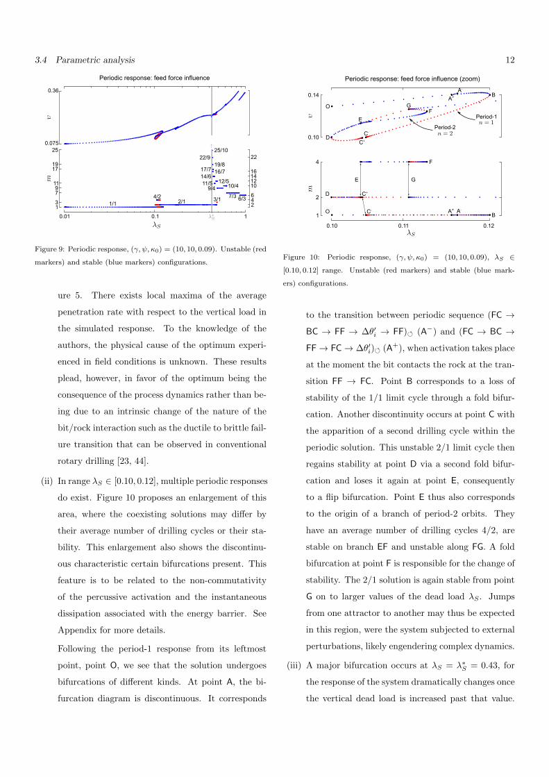
(ii) In range λS ∈ [0.10, 0.12], multiple periodic responses

do exist. Figure 10 proposes an enlargement of this

area, where the coexisting solutions may differ by

their average number of drilling cycles or their sta-

bility. This enlargement also shows the discontinu-

ous characteristic certain bifurcations present. This

feature is to be related to the non-commutativity

of the percussive activation and the instantaneous

dissipation associated with the energy barrier. See

Appendix for more details.

Following the period-1 response from its leftmost

point, point O, we see that the solution undergoes

bifurcations of different kinds. At point A, the bi-

furcation diagram is discontinuous. It corresponds

0.10 0.12

4

2

1

Periodic response: feed force influence (zoom)

F

D

E

A-

A+ B

C+

C-

G

B

E

C+

C-

D

G

F

A-A+

0.11

0.14

0.10

Period-2

Period-1

O

O

Figure 10: Periodic response, (γ, ψ, κ0) = (10, 10, 0.09), λS ∈

[0.10, 0.12] range. Unstable (red markers) and stable (blue mark-

ers) configurations.

to the transition between periodic sequence (FC →

BC → FF → ∆θ′i → FF) (A−) and (FC → BC →

FF→ FC→ ∆θ′i) (A+), when activation takes place

at the moment the bit contacts the rock at the tran-

sition FF → FC. Point B corresponds to a loss of

stability of the 1/1 limit cycle through a fold bifur-

cation. Another discontinuity occurs at point C with

the apparition of a second drilling cycle within the

periodic solution. This unstable 2/1 limit cycle then

regains stability at point D via a second fold bifur-

cation and loses it again at point E, consequently

to a flip bifurcation. Point E thus also corresponds

to the origin of a branch of period-2 orbits. They

have an average number of drilling cycles 4/2, are

stable on branch EF and unstable along FG. A fold

bifurcation at point F is responsible for the change of

stability. The 2/1 solution is again stable from point

G on to larger values of the dead load λS . Jumps

from one attractor to another may thus be expected

in this region, were the system subjected to external

perturbations, likely engendering complex dynamics.

(iii) A major bifurcation occurs at λS = λ∗S = 0.43, for

the response of the system dramatically changes once

the vertical dead load is increased past that value.

13

This bifurcation corresponds to the appearance of a

standstill phase in the periodic sequence. Confirma-

tion of this abrupt change of behavior is given by the

stroboscopic Poincare map of the system (Figure 11)

that depicts the state of the system prior to impact.

On the map is also visible the change of periodicity

of the limit cycle as λS varies.

Stroboscopic Poincaré Map

1.95

0.00

-0.66

0.01 0.1 1

0.72

0.00

-0.22

Figure 11: Stroboscopic Poincare map at τ = τ−i , (γ, ψ, κ0) =

(10, 10, 0.09). The map displays 500 points that were sampled af-

ter removal of a transient of 500 periods. The system was initialized

in standstill phase.

At the bifurcation point, the number of drilling cy-

cles increases dramatically. Numerics nonetheless

show that this increase verifies a bounded average

number of drilling cycles as it remains in the range

[2, 3] observed on the nearby branches correspond-

ing to periodic solutions without standstill. Past the

bifurcation, for λS ∈ [λ∗S , 1], discontinuities of the

average rate of penetration follow from changes in

the periodic sequence.

4. Conclusion

In this paper, we have presented a low dimension model

for the study of the process of percussive drilling. This

novel model combines elements previously studied in the

literature but that, to the knowledge of the authors, had

not been assembled before: a drifting oscillator impulsively

loaded coupled with a bilinear bit/rock interaction law,

together with an energy barrier. The assembly of these

building blocks has resulted in a hybrid dynamical sys-

tem governed by four drilling phases and associated mode

transition conditions.

A preliminary analysis of the model has shown the

necessity of complementing the bilinear force/penetration

law by an energy barrier to differentiate the cases of static

and dynamic indentations and prevent unbounded pene-

tration under static loading. Consequent to the energy

barrier is an instantaneous dissipation of kinetic energy at

the moment the bit contacts the rock. This analysis has

also shed light on some expected behaviors of the system.

In particular, the standstill phase has been shown to be

an absorbant element of the dynamical system, acting as

a reset of the initial conditions.

Results of numerical simulations by use of techniques

tailored to hybrid systems have revealed three main facts.

First, the model appears to recover an experimentally-

observed trend; that is, the existence of local maxima of

the average steady-state penetration rate with respect to

the vertical load on bit. Second, for given ranges of the ver-

tical load, the studied configurations exhibit coexistence

of stable and unstable limit cycles. Complex responses are

likely to be observed in these regions. Third, at larger

loads, periodic solutions comprise a standstill phase; that

is, the bit performs a certain number of drilling cycles un-

der the percussive activation before coming to rest until

the next activation takes place.

Similarly to the results obtained by Ajibose et al. [29],

our analysis also shows evidence of the existence of an

optimum drilling configuration. There are, however, fun-

damental differences between the two drifting oscillator

models of the drilling process. First, our model relies on

an impulsive activation while theirs is based on a harmonic

one; second, the bilinear interface law we propose incorpo-

rates an energy barrier, while the polynomial laws they use

do not. These choices limit the applicability of the models

to certain parameter ranges, ranges that may be related to

14

the technology the model is associated with. In particular,

our model attempts at representing percussive drilling (im-

pulsive activation at frequencies O(10) Hz) whereas theirs

is aimed at describing ultrasonic drilling and machining

(high frequency harmonic activation at a frequencies O(1)

kHz).

Further investigations are required to deeper under-

stand the dynamics of the process described by the pro-

posed model, in addition to the comprehension of the bi-

furcations taking place in the system when parameters are

swept. More specifically, we expect the understanding of

the dynamics to lead to the identification of the conditions

related to optimal drilling.

Acknowledgments

This research was supported by the Commonwealth

Scientific and Industrial Research Organisation (CSIRO)

and by Itasca International Inc. These supports are grate-

fully acknowledged.

References

[1] P.A. Bartelt, W. Ammann, and E. Anderheggen. The numerical

simulation of the impact phenomena in nail penetration. Nucl.

Eng. Des., 150:431–440, 1994.

[2] P. Villaggio. Hammering of Nails and Pitons. Math. Mech.

Solids, 10(4):461–468, August 2005.

[3] P. Kettil, G. Engstrom, and N. Wiberg. Coupled simulation of

wave propagation and water pumping phenomenon in driven

concrete piles. Comput. Struct., 85(3-4):170–178, February

2007.

[4] U.V. Le. A general mathematical model for the collision be-

tween a free-fall hammer of a pile-driver and an elastic pile:

Continuous dependence and low-frequency asymptotic expan-

sion. Nonlinear Anal.-Real., 12(1):702–722, February 2011.

[5] L. Zhou, J. Chen, and W. Lao. Construction Control and Pile

Body Tensile Stresses Distribution Pattern during Driving. J.

Geotech. Geoenviron., 133(9):1102–1109, 2007.

[6] G.L. Cavanough, M. Kochanek, J.B. Cunningham, and I.D.

Gipps. A Self-Optimizing Control System for Hard Rock Per-

cussive Drilling. IEEE-ASME T. Mech., 13(2):153–157, April

2008.

[7] L.E. Chiang and D.A. Elias. Modeling impact in down-the-hole

rock drilling. Int. J. Rock Mech. Min., 37(4):599–613, June

2000.

[8] E. Nordlund. The Effect of Thrust on the Performance of Per-

cussive Rock Drills. Int. J. of Rock Mech. Min. Sci. Geomech.

Abstr., 26(I):51–59, 1989.

[9] W.A. Hustrulid and C.E. Fairhurst. Theoretical and Experi-

mental Study of Percussive Drilling of Rock - Part I - Theory

of Percussive Drilling. Int. J. Rock Mech. Min., 8(4):311–333,

July 1971.

[10] B.R. Stephenson. Measurement of Dynamic Force-Penetration

Characteristics in Indiana Limestone. Master’s thesis, Univer-

sity of Minnesota, 1963.

[11] B. Haimson. High Velocity, Low Velocity and Static Penetration

Characteristics in Tennessee Marble. Master’s thesis, Univer-

sity of Minnesota, 1965.

[12] W.A. Hustrulid and C.E. Fairhurst. Theoretical and Ex-

perimental Study of Percussive Drilling of Rock - Part II -

Force-Penetration and Specific Energy Determinations. Int.

J. Rock Mech. Min., 8(4):335–356, July 1971. doi: 10.1016/

0148-9062(71)90046-5.

[13] L.G. Karlsson, B. Lundberg, and K.G. Sundin. Experimental

study of a percussive process for rock fragmentation. Int. J.

Rock Mech. Min. Sci. Geomech. Abstr., 26(1):45–50, January

1989.

[14] S. Y. Wang, S. W. Sloan, H. Y. Liu, and C. A. Tang. Numerical

simulation of the rock fragmentation process induced by two

drill bits subjected to static and dynamic (impact) loading. Rock

Mech. Rock Eng., 44(3):317–332, November 2010.

[15] T. Saksala. Numerical modelling of bit–rock fracture mecha-

nisms in percussive drilling with a continuum approach. Int. J.

Numer. Anal. Meth. Geomech., 35:1483–1505, 2011.

[16] F. Zhang and H. Huang. Discrete Element Modeling of Sphere

Indentation in Rocks. In 45th US Rock Mechanics / Geome-

chanics Symposium, San Francisco, CA, U.S.A., 2011. American

Rock Mechanics Association.

[17] X. Li, G. Rupert, and D.A. Summers. Energy transmission

of down-hole hammer tool and its conditionality. T. Nonferr.

Metal Soc., 10(1):109–113, 2000.

[18] B. Lundberg. Microcomputer simulation of percussive drilling.

Int. J. Rock Mech. Min. Sci., 22(4):237–249, August 1985.

[19] A.M. Krivtsov and M. Wiercigroch. Dry friction model of per-

cussive drilling. Meccanica, 34(6):425–435, December 1999.

[20] A.M. Krivtsov and M. Wiercigroch. Penetration rate prediction

for percussive drilling via dry friction model. Chaos Soliton.

Fract., 11(15):2479–2485, December 2000.

[21] E. Pavlovskaia, M. Wiercigroch, and C. Grebogi. Modeling of

an impact system with a drift. Phys. Rev. E, 64:56224–56229,

15

November 2001.

[22] H. Alehossein, E. Detournay, and H. Huang. An Analytical

Model for the Indentation of Rocks by Blunt Tools. Rock Mech.

and Rock Eng., 33(4):267–284, 2000.

[23] H. Huang and E. Detournay. Intrinsic Length Scales in Tool-

Rock Interaction. Int. J. Geomech., 8(1):39–44, 2008.

[24] O.K. Ajibose. Nonlinear Dynamics and Contact Fracture Me-

chanics of High Frequency Percussive Drilling. Ph.D. thesis,

University of Aberdeen, 2009.

[25] W. Changming. An analytical study of percussive energy trans-

fer in hydraulic rock drills. Min. Sci. Technol., 13(1):57–68,

July 1991.

[26] M. Amjad. Control of ITH Percussive Longhole Driling in

Hard Rock. Ph.D. thesis, McGill University, Montreal, Quebec,

Canada, 1996.

[27] G. Pearse. Hydraulic rock drills. Min. Mag., pages 220–231,

March 1985.

[28] O.K. Ajibose, M. Wiercigroch, E. Pavlovskaia, and A.R. Ak-

isanya. Contact force models and the dynamics of drifting im-

pact oscillator. In V Denoel and E Detournay, editors, First

International Colloquium on Non-Linear Dynamics of Deep

Drilling Systems, pages 33–38, 2009.

[29] O. K. Ajibose, M. Wiercigroch, E. Pavlovskaia, A. R. Akisanya,

and G Karolyi. Drifting Impact Oscillator With a New Model

of the Progression Phase. J. Appl. Mech., 79(6):061007–1–9,

November 2012.

[30] M. di Bernardo, C.J. Budd, A.R. Champneys, and P. Kowal-

czyk. Piecewise-smooth Dynamical Systems - Theory and Ap-

plications, volume 163. Springer-Verlag London Ltd., 2008.

[31] R.I. Leine and H. Nijmeijer. Dynamics and Bifurcations of Non-

Smooth Mechanical Systems. Springer-Verlag Berlin Heidelberg,

2004.

[32] R.I. Leine. Bifurcations of equilibria in non-smooth continuous

systems. Physica D, 223(1):121–137, November 2006.

[33] G. Luo and J. Xie. Bifurcations and chaos in a system with

impacts. Physica D, 148(3-4):183–200, January 2001.

[34] J.J.P. Veermana, D. Daescua, M.J. Romero-Vallesb, and P.J.

Torres. A single particle impact model for motion in avalanches.

Physica D, 238(19):1897–1908, 2009.

[35] B. Lundberg and M. Okrouhlik. Efficiency of a percussive rock

drilling process with consideration of wave energy radiation into

the rock. International Journal of Impact Engineering, 32:

1573–1583, 2006.

[36] V. Acary and B. Brogliato. Numerical Methods for Nonsmooth

Dynamical Systems. Applications in Mechanics and Electron-

ics. Springer Verlag Berlin Heidelberg, 2008.

[37] A.H. Nayfeh and B. Balachandran. Applied Nonlinear Dy-

namics: Analytical, Computational and Experimental Methods.

Wiley-VCH Verlag GmbH and Co. KGaA, Weinheim, 1995.

[38] R. Seydel. Practical bifurcation and stability analysis. Springer

New York Dordrecht Heidelberg London, 2009.

[39] A.M.P. Valli, R.N. Elias, G.F. Carey, and A.L.G.A. Coutinho.

PID adaptive control of incremental and arclength continuation

in nonlinear applications. Int. J. Numer. Meth. Fl., 61:1181–

1200, 2009.

[40] J. Awrejcewicz and C.-H. Lamarque. Bifurcation And Chaos

In Nonsmooth Mechanical Systems. World Scientific Publishing

Co., 2003.

[41] A. Depouhon, E. Detournay, and V. Denoel. Limit Cycling Be-

havior of a Hybrid System: Application to Percussive Drilling.

In N. van de Wouw and E. Detournay, editors, Second Inter-

national Colloquium on Non-Linear Dynamics and Control of

Deep Drilling Systems, pages 77–86, 2012.

[42] F. Peterka and J. Vacik. Transition to chaotic motion in me-

chanical systems with impacts. Journal of Sound and Vibration,

154(1):95–115, 1992.

[43] F. Peterka. Dynamics of Double Impact Oscillators. Facta Univ.

Ser. Mech. Automat. Control Robot., 2(10):1177–1190, 2000.

[44] T. Richard. Determination of rock strength from cutting tests.

M.S. thesis, University of Minnesota, 1999.

A. Non-commutativity of the percussive activation

and energy barrier

To illustrate the reason underlying the discontinuities

of the bifurcation diagram along the branches correspond-

ing to periodic orbits without standstill phase, we con-

sider the one occurring at point A of Figure 9. Left of

it (λS < λS |A− , branch OA−), the periodic sequence is

given by (FC → BC → FF → ∆θ′i → FF). Right of it

(λS > λS |A+ , branch A+B), it is (FC → BC → FF →

FC → ∆θ′i). Thus, the limiting case corresponds to the

periodic sequence (FC→ BC→ FF→ ∆θ′i) and must be

considered for a vanishing FF (A−) or FC (A+) phase.

Starting with the A− case, we write the periodicity

conditions of the orbit by following its periodic sequence,

from initial conditions (0, θ′`) in FC phase, i.e. before the

energy barrier is applied. It reads

θ′` =

√θ′`

2 − κ20γ

+ 1, (28)

16

and

ψ =

(1 +

1√γ

)(π − acos

λS√λ2S + θ′`

2 − κ20

)· · ·

· · ·+ 2

λS

√θ′`

2 − κ20γ

. (29)

While the former equation has a closed-form solution

θ′` =

√γ

γ − 1

(√γ +

√1− γ − 1

γκ20

), (30)

the latter requires a numerical resolution. Considering the

numerical parameters of the bifurcation analysis, namely

(γ, ψ, κ0) = (10, 10, 0.09), we find

(λS , θ′`) = (0.1178, 1.4610). (31)

Then we write the periodicity conditions assuming the

activation no longer takes place during the FF phase but

during the FC one. They read

θ′` =1√γ

(√θ′`

2 − κ20 + 1

), (32)

ψ =

(1 +

1√γ

)π − acos

λS√λ2S +

(√θ′`

2 − κ20 + 1)2

+2

λS

√θ′`

2 − κ20 + 1√γ

. (33)

Again, the first condition can be solved analytically for the

velocity

θ′` =1

γ − 1

(√γ +

√1− (γ − 1)κ20

)(34)

but the second requires a numerical procedure to be solved

for λS . Using the numerical parameters of the bifurcation

analysis, we obtain

(λS , θ′`) = (0.1170, 0.4579) (35)

which is different from result (31). The limiting behaviors

from the left and from the right are thus different, and

this difference stems from the non-commutativity of the

percussive activation and the energy barrier with respect

to periodic responses of the system.

Discontinuities of the bifurcation diagram are therefore

expected whenever the activation passes from a FF phase

to a FC one, and when a new drilling cycle appears in the

periodic sequence, through a BC → ∆θi → FC transition.

Should κ0 = 0, the bifurcation diagram of Figure 10 would

then be continuous at points A and C.