A double-layered nonlinear model predictive control based

Wang et al. / Front Inform Technol Electron Eng 2020 21(7):1059-1073 1059

A double-layered nonlinear model predictive control based control algorithm for local trajectory planning for automated trucks under

uncertain road adhesion coefficient conditions*

Hong-chao WANG1, Wei-wei ZHANG‡1, Xun-cheng WU1, Hao-tian CAO2, Qiao-ming GAO3, Su-yun LUO1

1College of Mechanical and Automotive Engineering, Shanghai University of Engineering Science, Shanghai 201620, China 2State Key Laboratory of Advanced Design and Manufacturing for Vehicle Body, Hunan University, Changsha 410082, China

3College of Automobile and Transportation, Guangxi University of Science and Technology, Liuzhou 545006, China E-mail: [email protected]; [email protected]; [email protected];

[email protected]; [email protected]; [email protected] Received Apr. 8, 2019; Revision accepted Sept. 16, 2019; Crosschecked June 3, 2020

Abstract: We present a double-layered control algorithm to plan the local trajectory for automated trucks equipped with four hub motors. The main layer of the proposed control algorithm consists of a main layer nonlinear model predictive control (MLN-MPC) controller and a secondary layer nonlinear MPC (SLN-MPC) controller. The MLN-MPC controller is applied to plan a dynami-cally feasible trajectory, and the SLN-MPC controller is designed to limit the longitudinal slip of wheels within a stable zone to avoid the tire excessively slipping during traction. Overall, this is a closed-loop control system. Under the off-line co-simulation environments of AMESim, Simulink, dSPACE, and TruckSim, a dynamically feasible trajectory with collision avoidance opera-tion can be generated using the proposed method, and the longitudinal wheel slip can be constrained within a stable zone so that the driving safety of the truck can be ensured under uncertain road surface conditions. In addition, the stability and robustness of the method are verified by adding a driver model to evaluate the application in the real world. Furthermore, simulation results show that there is lower computational cost compared with the conventional PID-based control method. Key words: Automated truck; Trajectory planning; Nonlinear model predictive control; Longitudinal slip https://doi.org/10.1631/FITEE.1900185 CLC number: TP273

1 Introduction

As an emerging technology, autonomous trucks (ATs) have the potential to improve the efficiency of land transportation. In the USA, the first autonomous cargo truck made by Uber was officially launched in 2016, reported by Wired (https://www.wired. com/2016/10/ubers-self-driving-truck-makes-first- delivery-50000-beers/). Furthermore, in recent years, the surge in trade has an increasing demand for trucking and truck drivers (Mittal et al., 2018). Therefore, the development of ATs is an urgent and reasonable project. In addition, the research on bat-tery technology has made electric trucks technically

Frontiers of Information Technology & Electronic Engineering www.jzus.zju.edu.cn; engineering.cae.cn; www.springerlink.com ISSN 2095-9184 (print); ISSN 2095-9230 (online) E-mail: [email protected]

‡ Corresponding author * Project supported by the National Fund for Fundamental Research, China (No. 282017Y-5303), the National Natural Science Foundation of China (Nos. 51805312 and 51675324), the Shanghai Sailing Pro-gram, China (No. 18YF1409400), the Training and Funding Program of Shanghai College Young Teachers, China (No. ZZGCD15102), the Scientific Research Project of Shanghai University of Engineering Science, China (No. 2016-19), the Shanghai University of Engineering Science Innovation Fund for Graduate Students, China (No. 18KY0610), and the Technology and Innovation Projects of Guangxi Province, China (No. 2017-393)

ORCID: Hong-chao WANG, https://orcid.org/0000-0002-9190- 179X; Wei-wei ZHANG, https://orcid.org/0000-0002-9768-2620 © Zhejiang University and Springer-Verlag GmbH Germany, part of Springer Nature 2020

Administrator

新建图章

http://crossmark.crossref.org/dialog/?doi=10.1631/FITEE.1900185&domain=pdf


and commercially feasible (Mareev et al., 2018), so truck electrification is an interesting research area.

Many algorithms have been presented for con-trolling vehicle wheel slip (Amodeo et al., 2010). An adaptive wheel control algorithm based on slip opti-mization was developed by Kim J and Lee (2018) to trade off the conflict between maximizing traction and minimizing energy consumption. A control algo-rithm was developed with a wheel slip controller based on the sliding mode framework to improve the electric vehicle safety (de Castro et al., 2013). In addition, to optimize energy efficiency and dynamic performance, the braking torques among two actua-tors can be distributed by the algorithm proposed by de Castro et al. (2012), which relies on a wheel torque allocator and a robust adaptive wheel slip controller.

As in autonomous cars, trajectory planning ca-pability is a key for ATs. Local trajectory planning for ATs requires an accurate and difficult decision in real time based on ATs’ kinematically and dynamically feasible limits and lane boundaries (Katrakazas et al., 2015). Many local trajectory planning methods adopt mainly one of the following noted techniques: poten-tial fields, cell decomposition, and optimal control (Dixit et al., 2018).

Glaser et al. (2010) proposed that the potential field algorithms assign repulsive forces to obstacles and attractive forces to a safe region of the vehicle and compute trajectories along the steepest gradient in the resulting potential field, including artificial potential fields (Barraquand et al., 1992) and vector field his-tograms (Borenstein and Koren, 1991). The algorithm proposed by Kitazawa and Kaneko (2017) was ex-perimentally verified for only low-speed maneuvers, because it depends seriously on the accuracy of the generated potential field. Additionally, kinematic constraints of the vehicle cannot be handled perfectly, which may cause safety issues during high-speed traveling scenarios (Shim et al., 2012). Cell decom-position algorithms such as rapidly exploring random tree (RRT) are applied to plan collision-free paths. However, the computational complexity of the methodology may increase traffic density. Further-more, on-board computing on busy roads is increas-ingly jeopardized (Ma et al., 2014). An optimal con-trol algorithm minimizing mainly a performance in-dex such as kinetic energy change (Shamir, 2004), jerk (Chu et al., 2012), or lateral acceleration (Shim

et al. 2012) is applied to obtain a feasible trajectory to execute the overtaking maneuver. Experimental re-sults in Chu et al. (2012) and Shim et al. (2012) demonstrated that the algorithm can generate collision-free trajectories with low computational requirements.

The model predictive control (MPC) method, an algorithm that can address system constraints and nonlinearities, has been used for local trajectory planning in many state-of-the-art vehicles. Re-searchers have tried to reduce the computational complexity using a point mass vehicle model (Kim B et al., 2016) and a linear kinematic bicycle vehicle model (Gao YQ et al., 2014). Researchers have pro-posed many solutions to address this problem such as translating the problem from a time-dependent system to a position-dependent system (Gao Y et al., 2012), relaxing collision avoidance constraints (Nilsson et al., 2014), and approximate linearization (Carvalho et al., 2013). However, these solutions require accu-rate knowledge of the states (such as obstacles and computing platform performance). Cesari et al. (2017) demonstrated that the computing constraint problem can be addressed with a real-time prototyping system, but it is still difficult to generate a dynamically fea-sible trajectory in the real world.

Note that all algorithms mentioned above were executed under the assumption that the exact knowledge of the environment is known in the tra-jectory planning system. However, in the real world, the system may be disturbed by information errors such as road surface conditions and weather condi-tions (Dixit et al., 2018). These errors may impact ego vehicle’s dynamic limits and even its safety. The system constraint, especially for road surface condi-tion, is a key influence factor affecting the dynamic and safety performance of the vehicle in the path- planner system. Researchers always consider it an accurately known constant when considering the constraint of road surface adhesion conditions, but the road adhesion coefficients between the right and left sides of the vehicle may be different in a real envi-ronment. So, the generated trajectory may not be able to satisfy vehicle’s dynamics and safety requirements. Therefore, uncertain road conditions, especially in rainy or snowy weather, may cause a vehicle to slip longitudinally or laterally, and should be considered in the trajectory planning system. To present the


properties of longitudinal or lateral tire forces, a three-directional coupled vehicle-road system was developed by Li and Yang (2015). To obtain more realistic vehicle trajectories for estimating vehicle safety measures, a vehicle dynamics model-integrated simulation was developed by CarSim (So et al., 2014). A framework for designing and operating a global production network was introduced by Lanza et al. (2019), which is a useful application in the intelligent transportation industry.

Therefore, to limit the longitudinal slip of wheels within a stable zone to avoid the tire excessively slipping during traction and to generate a dynamically feasible trajectory, a double-layered nonlinear MPC algorithm is proposed, consisting of a main layer nonlinear MPC (MLN-MPC) controller and a sec-ondary layer nonlinear MPC (SLN-MPC) controller. The MLN-MPC controller is applied to plan the tra-jectory features of two system inputs: one is the yaw rate of the truck and the other is truck acceleration. The real-time information of the yaw rate can be eas-ily obtained by sensors, and the acceleration is de-termined by the hub motor torque. This torque is one of the system inputs of the SLN-MPC controller be-cause the ego truck is driven by four hub motors. Considering an uncertain road adhesion coefficient, the SLN-MPC controller is designed to limit the lon-gitudinal slip of four wheels within a stable zone to ensure truck safety, making these control issues time-domain constraints of a nonlinear MPC problem. The trajectories generated from the double-layered nonlinear MPC algorithm have been verified with respect to the effectiveness of the truck longitudinal slip and lateral acceleration by a co-simulation using AMESim, Simulink, dSPACE, and TruckSim soft-ware. Furthermore, to verify the stability and ro-bustness of the proposed method, a driver model has been added to evaluate the application in the real world. To evaluate the computational complexity and efficiency of the algorithm, the computational time of these methods is addressed in simulation. 2 Determination of the output torque for hub motors in the SLN-MPC controller

For vehicles driven by hub motors, the actual hub motor output torque is a direct factor in deter-mining the magnitude of a truck’s acceleration.

Therefore, it is necessary to control the output torque of the hub motors before designing the MLN-MPC controller. In this section, we focus mainly on con-trolling motor’s torque by constraining the longitu-dinal slip of the truck within a stable zone as a control target. Therefore, before designing the motor output torque controller, it is necessary to describe the lon-gitudinal slip model of the vehicle.

2.1 Vehicle longitudinal slip control model

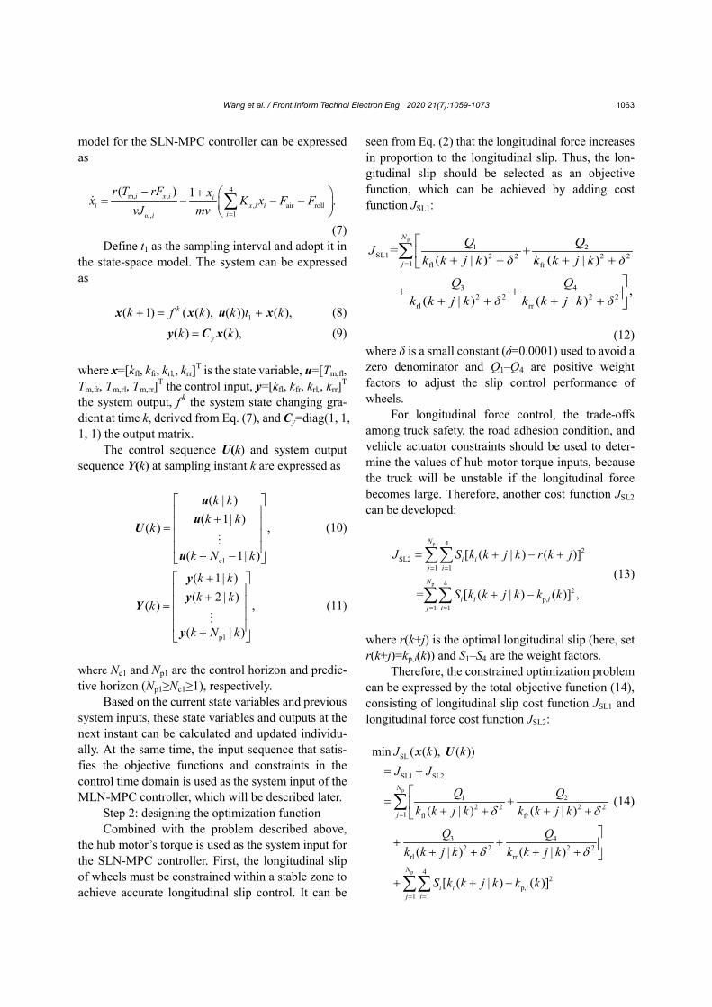
Because real-time road surface condition in-formation is a key factor affecting the dynamics and safety performance of the vehicle in the path-planner system, it cannot be ignored in real-world applica-tions. However, the real-time road adhesion coeffi-cient is usually hard to accurately detect. To address this problem, a longitudinal slip control model is built into the path-planner system. Furthermore, the tire slip level can influence the force, and can be ex-pressed by the wheel angular velocity (ω), vehicle velocity (v), and tire rolling radius (r), denoted as

, fl, fr, rl, rr,max( , )

−= =i

iv ω r

k iv η

(1)

where η is a small constant which is set to 0.15 m/s (after simulation comparison), avoiding a zero de-nominator and other numerical problems such as the fact that ki→∞ is incompatible with the tire charac-teristics, and fl, fr, rl, and rr represent the front left, front right, rear left, and rear right wheels, respectively.

Considering that the value of the slip ki should be kept small (approximately, ki=0−0.03) to improve tire durability and ensure vehicle safety, and that the tire model is approximately linear when ki is small, the tire model can be formulated as a linear approxima-tion based on the slip limitation and tire magic for-mula model. After linear approximation, the longitu-dinal force can be expressed as

, , , , fl, fr, rl, rr,x i x i x iF K k i= = (2)

where Fx is the longitudinal force, Kx the longitudinal slip stiffness, and kx the longitudinal tire slip.

The direct permanent magnet synchronous mo-tor (PMSM) is selected as the hub motor model in this study, because it has a good power factor, slightly


high efficiency, and low torque ripple or noise (Las-karis and Kladas, 2010). The motor’s maximum power is 75 kW and its maximum torque is 1000 N∙m. To provide the required torque to the torque controller, the desired motor’s closed-loop dynamics can be denoted as

m c1 ,

1T T

τs=

+ (3)

where τ=20 s is the close-loop response time, s the time function, and Tc the motor command torque.

Constraints of the actuators in the truck should be considered, especially the physical constraints of the hub motors. As a significant factor in determining the magnitude of truck acceleration, the motor com-mand torque Tc should be limited by the maximum torque of the motor, expressed as

m,max c m,max .T T T− ≤ ≤ (4)

Therefore, the wheel longitudinal slip ratio dy-

namics can be expressed as

m, ,

,

,fl ,fr ,rl ,rr air roll

( ) 1

( ),

i x i ii

i

x x x x

r T rF kkvJ mv

F F F F F Fω

− += −

⋅ + + + − −

(5)

where m is the total mass of the vehicle, Jω,i the mo-ment of inertia of the four wheels, Fair the force of air resistance, and Froll the force of rolling resistance.

In addition, the road adhesion coefficient be-tween the tire and road surface is closely related to the longitudinal slip of the wheels (Mutoh, 2012). Fig. 1 depicts the relationship between the road adhesion coefficient and the longitudinal slip of the wheels. It can be seen from Fig. 1 that the longitudinal slip is in the nonlinear region and that it is difficult to achieve precise control of an unstable tire (|k|>kp) in the real world. Thus, the longitudinal slip of each wheel should be limited to a stable zone to ensure that the tire is within a linear region and to avoid the wheel spinning out under slippery road conditions, ex-pressed as

max max max p, .k k k k k− ≤ ≤ = (6)

2.2 Design of the SLN-MPC longitudinal slip controller

Nonlinear MPC is an algorithm that uses a model to predict the future dynamics of a controlled plant. At each sampling time, based on the current measure-ment information, a finite time-domain open-loop optimization problem is solved online, and the first element of the obtained control sequence is applied to the controlled object. At the next sampling instant, the optimization problem is refreshed with the newly measured value and is resolved (Chen, 2013). Three steps can be included to briefly describe the algo-rithm’s principle, i.e., predicting the future states of a system, solving the optimization problem, and ap-plying the first element of the optimized solution to the system.

Note that these steps are executed repeatedly at each sampling time. Furthermore, the measurements obtained at each sampling instant will be used as the initial conditions for predicting future states regard-less of the model that is used.

Therefore, before designing the SLN-MPC con-troller, the control requirements that the control sys-tem must meet include limiting the longitudinal slip within the stable zone (Fig. 1) and limiting the motor torque according to constraint (4), so the design of the SLN-MPC controller can be implemented mainly in two steps:

Step 1: establishing a time-based discretized model

To obtain a finite-dimensional optimization control problem, the Euler method is used to discre-tize the system’s state-space model, so the state-space

Fig. 1 Relationship between the road adhesion coefficient and the longitudinal slip

Longitudinal adhesion coefficient μx

Stable Unstable

Lateral adhesion coefficient μy

Longitudinal slip k

Adh

esio

n co

effic

ient

kp

μx,max


model for the SLN-MPC controller can be expressed as

4m, ,

, air roll1,

( ) 1.i x i i

i x i iiω i

r T rF xx K x F FvJ mv =

− + = − − −

∑

(7) Define t1 as the sampling interval and adopt it in

the state-space model. The system can be expressed as

1( 1) ( ( ), ( )) ( ),kk f k k t k+ = +x x u x (8)

( ) ( ),yk k=y C x (9)

where x=[kfl, kfr, krl,, krr]T is the state variable, u=[Tm,fl, Tm,fr, Tm,rl, Tm,rr]T the control input, y=[kfl, kfr, krl,, krr]T the system output, f

k the system state changing gra-dient at time k, derived from Eq. (7), and Cy=diag(1, 1, 1, 1) the output matrix.

The control sequence U(k) and system output sequence Y(k) at sampling instant k are expressed as

c1

( | )( 1| )

( ) ,

( 1| )

k kk k

k

k N k

+ = + −

uu

U

u

(10)

p1

( 1| )( 2 | )

( ) ,

( | )

k kk k

k

k N k

+ + = +

yy

Y

y

(11)

where Nc1 and Np1 are the control horizon and predic-tive horizon (Np1≥Nc1≥1), respectively.

Based on the current state variables and previous system inputs, these state variables and outputs at the next instant can be calculated and updated individu-ally. At the same time, the input sequence that satis-fies the objective functions and constraints in the control time domain is used as the system input of the MLN-MPC controller, which will be described later.

Step 2: designing the optimization function Combined with the problem described above,

the hub motor’s torque is used as the system input for the SLN-MPC controller. First, the longitudinal slip of wheels must be constrained within a stable zone to achieve accurate longitudinal slip control. It can be

seen from Eq. (2) that the longitudinal force increases in proportion to the longitudinal slip. Thus, the lon-gitudinal slip should be selected as an objective function, which can be achieved by adding cost function JSL1:

p

1 2SL1 2 2 2 2

1 fl fr

3 42 2 2 2

rl rr

=( | ) ( | )

,( | ) ( | )

N

j

Q QJk k j k δ k k j k δ

Q Qk k j k δ k k j k δ

=

+ + + + +

+ + + + + +

∑

(12)

where δ is a small constant (δ=0.0001) used to avoid a zero denominator and Q1–Q4 are positive weight factors to adjust the slip control performance of wheels.

For longitudinal force control, the trade-offs among truck safety, the road adhesion condition, and vehicle actuator constraints should be used to deter-mine the values of hub motor torque inputs, because the truck will be unstable if the longitudinal force becomes large. Therefore, another cost function JSL2 can be developed:

p

p

42

SL21 1

42

p,1 1

[ ( | ) ( )]

= [ ( | ) ( )] ,

N

i ij i

N

i i ij i

J S k k j k r k j

S k k j k k k

= =

= =

= + − +

+ −

∑∑

∑∑ (13)

where r(k+j) is the optimal longitudinal slip (here, set r(k+j)=kp,i(k)) and S1–S4 are the weight factors.

Therefore, the constrained optimization problem can be expressed by the total objective function (14), consisting of longitudinal slip cost function JSL1 and longitudinal force cost function JSL2:

p

p

SL

SL1 SL2

1 22 2 2 2

1 fl fr

3 42 2 2 2

rl rr

42

p,1 1

min ( ( ), ( ))

( | ) ( | )

( | ) ( | )

[ ( | ) ( )]

N

j

N

i i ij i

J k kJ J

Q Qk k j k k k j k

Q Qk k j k k k j k

S k k j k k k

δ δ

δ δ

=

= =

= +

= + + + + +

+ + + + + +

+ + −

∑

∑∑

x U

(14)


c, m,max ps.t. ( | ) , 1, 2, ..., ,iT k j k T j N+ ≤ = (15)

where i∈{fl, fr, rl, rr}.

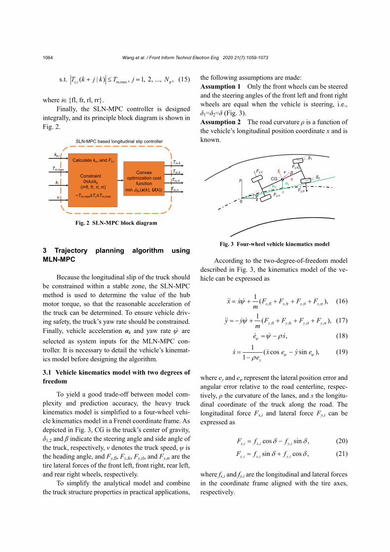
Finally, the SLN-MPC controller is designed integrally, and its principle block diagram is shown in Fig. 2.

3 Trajectory planning algorithm using MLN-MPC

Because the longitudinal slip of the truck should be constrained within a stable zone, the SLN-MPC method is used to determine the value of the hub motor torque, so that the reasonable acceleration of the truck can be determined. To ensure vehicle driv-ing safety, the truck’s yaw rate should be constrained. Finally, vehicle acceleration αk and yaw rate ψ are selected as system inputs for the MLN-MPC con-troller. It is necessary to detail the vehicle’s kinemat-ics model before designing the algorithm.

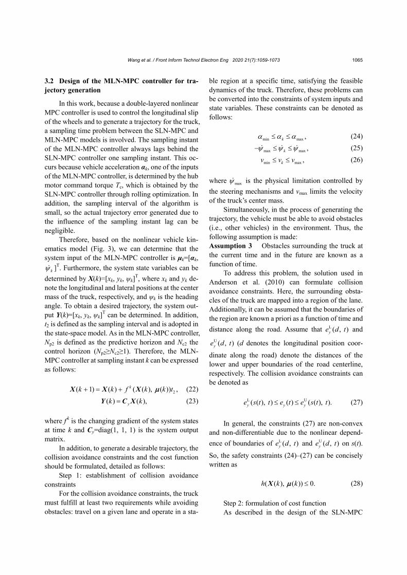
3.1 Vehicle kinematics model with two degrees of freedom

To yield a good trade-off between model com-plexity and prediction accuracy, the heavy truck kinematics model is simplified to a four-wheel vehi-cle kinematics model in a Frenét coordinate frame. As depicted in Fig. 3, CG is the truck’s center of gravity, δ1,2 and β indicate the steering angle and side angle of the truck, respectively, ν denotes the truck speed, ψ is the heading angle, and Fy,fl, Fy,fr, Fy,rl, and Fy,rr are the tire lateral forces of the front left, front right, rear left, and rear right wheels, respectively.

To simplify the analytical model and combine the truck structure properties in practical applications,

the following assumptions are made: Assumption 1 Only the front wheels can be steered and the steering angles of the front left and front right wheels are equal when the vehicle is steering, i.e., δ1=δ2=δ (Fig. 3). Assumption 2 The road curvature ρ is a function of the vehicle’s longitudinal position coordinate x and is known.

According to the two-degree-of-freedom model

described in Fig. 3, the kinematics model of the ve-hicle can be expressed as

,fl ,fr ,rl ,rr1 ( ),x x x xx x F F F Fm

ψ= + + + + (16)

,fl ,fr ,rl ,rr1 ( ),y y y yy y F F F Fm

ψ= − + + + + (17)

,e s= − ψ ψ ρ (18)

1 ( cos sin ),1 y

s x e y ee ψ ψρ

= −−

(19)

where ey and eψ represent the lateral position error and angular error relative to the road centerline, respec-tively, ρ the curvature of the lanes, and s the longitu-dinal coordinate of the truck along the road. The longitudinal force Fx,i and lateral force Fy,i can be expressed as

, , ,cos sin ,x i x i y iF f fδ δ= − (20)

, , ,sin cos ,y i x i y iF f fδ δ= + (21)

where fx,i and fy,i are the longitudinal and lateral forces in the coordinate frame aligned with the tire axes, respectively.

Fig. 2 SLN-MPC block diagram

SLN-MPC based longitudinal slip controller

Calculate kx,i and Fx,i

Constraint0≤ki≤kp

Convex optimization cost

function

−Tm,max≤Tc≤Tm,max

(i=fl, fr, rl, rr) min JSL(x(k), U(k))

kp,i

Tm,max

ki

v

Tm,fl

Tm,fr

Tm,rl

Tm,rr Fy,frFy,rr

Fy,rl

Fy,fl

x

y

0ψ

eψey

s

x

yδ2

δ1

CGv β

Fig. 3 Four-wheel vehicle kinematics model


3.2 Design of the MLN-MPC controller for tra-jectory generation

In this work, because a double-layered nonlinear MPC controller is used to control the longitudinal slip of the wheels and to generate a trajectory for the truck, a sampling time problem between the SLN-MPC and MLN-MPC models is involved. The sampling instant of the MLN-MPC controller always lags behind the SLN-MPC controller one sampling instant. This oc-curs because vehicle acceleration αk, one of the inputs of the MLN-MPC controller, is determined by the hub motor command torque Tc, which is obtained by the SLN-MPC controller through rolling optimization. In addition, the sampling interval of the algorithm is small, so the actual trajectory error generated due to the influence of the sampling instant lag can be negligible.

Therefore, based on the nonlinear vehicle kin-ematics model (Fig. 3), we can determine that the system input of the MLN-MPC controller is μk=[αk,

kψ ]T. Furthermore, the system state variables can be determined by X(k)=[xk, yk, ψk]T, where xk and yk de-note the longitudinal and lateral positions at the center mass of the truck, respectively, and ψk is the heading angle. To obtain a desired trajectory, the system out-put Y(k)=[xk, yk, ψk]T can be determined. In addition, t2 is defined as the sampling interval and is adopted in the state-space model. As in the MLN-MPC controller, Np2 is defined as the predictive horizon and Nc2 the control horizon (Np2≥Nc2≥1). Therefore, the MLN- MPC controller at sampling instant k can be expressed as follows:

2( 1) ( ) ( ( ), ( )) ,kk k f k k t+ = +X X X µ (22)

( ) ( ),yk k=Y C X (23) where f

k is the changing gradient of the system states at time k and Cy=diag(1, 1, 1) is the system output matrix.

In addition, to generate a desirable trajectory, the collision avoidance constraints and the cost function should be formulated, detailed as follows:

Step 1: establishment of collision avoidance constraints

For the collision avoidance constraints, the truck must fulfill at least two requirements while avoiding obstacles: travel on a given lane and operate in a sta-

ble region at a specific time, satisfying the feasible dynamics of the truck. Therefore, these problems can be converted into the constraints of system inputs and state variables. These constraints can be denoted as follows:

min max ,k≤ ≤a a a (24)

max max ,k− ≤ ≤ ψ ψ ψ (25) min max ,kv v v≤ ≤ (26)

where maxψ is the physical limitation controlled by the steering mechanisms and νmax limits the velocity of the truck’s center mass.

Simultaneously, in the process of generating the trajectory, the vehicle must be able to avoid obstacles (i.e., other vehicles) in the environment. Thus, the following assumption is made: Assumption 3 Obstacles surrounding the truck at the current time and in the future are known as a function of time.

To address this problem, the solution used in Anderson et al. (2010) can formulate collision avoidance constraints. Here, the surrounding obsta-cles of the truck are mapped into a region of the lane. Additionally, it can be assumed that the boundaries of the region are known a priori as a function of time and distance along the road. Assume that L ( , )ye d t and

U ( , )ye d t (d denotes the longitudinal position coor-

dinate along the road) denote the distances of the lower and upper boundaries of the road centerline, respectively. The collision avoidance constraints can be denoted as

L U( ( ), ) ( ) ( ( ), ).y y ye s t t e t e s t t≤ ≤ (27)

In general, the constraints (27) are non-convex

and non-differentiable due to the nonlinear depend-ence of boundaries of L ( , )ye d t and U ( , )ye d t on s(t).

So, the safety constraints (24)–(27) can be concisely written as

( ( ), ( )) 0.h k k ≤X µ (28)

Step 2: formulation of cost function As described in the design of the SLN-MPC


controller in Section 2, the nonlinear MPC problem can incorporate all objectives in one formula. The constrained optimization problem can be defined as follows:

p

FL

2 2d

0

2 2 21

min ( ( ), ( ))

( || || || ||

|| || || || )

N

v k α kk

j k k y k c y

J k k

ω ω

ω ω ψ ω=

−

= − +

+ − + +

∑

X U

v v α

α α e

(29)

2s.t. ( 1) ( ) ( ( ), ( )) ,kk k f k k t+ = +X X X µ (30)

p( ( ), ( )) 0, 0, 1,..., ,h k k k N≤ =X µ (31)

where ||νd−νk||2 adjusts the difference between the truck’s actual and desired velocities, ||αk||2 and ||αk−αk−1||2 are used to penalize the large control input and improve the truck’s dynamic stability, respec-tively, 2

kψ can avoid sharp increase in the yaw rate of the vehicle, ||ey||2 is used to penalize the large lateral position error, and ωi (i=ν, α, j, y, c) are the weighting factors.

Thus, the control principle of the MLN-MPC based controller block is designed (Fig. 4). The flowchart of the main steps of the mathematical ap-proach to the double-layer nonlinear MPC problem is shown in Fig. 5.

4 Simulation

4.1 Simulation environment

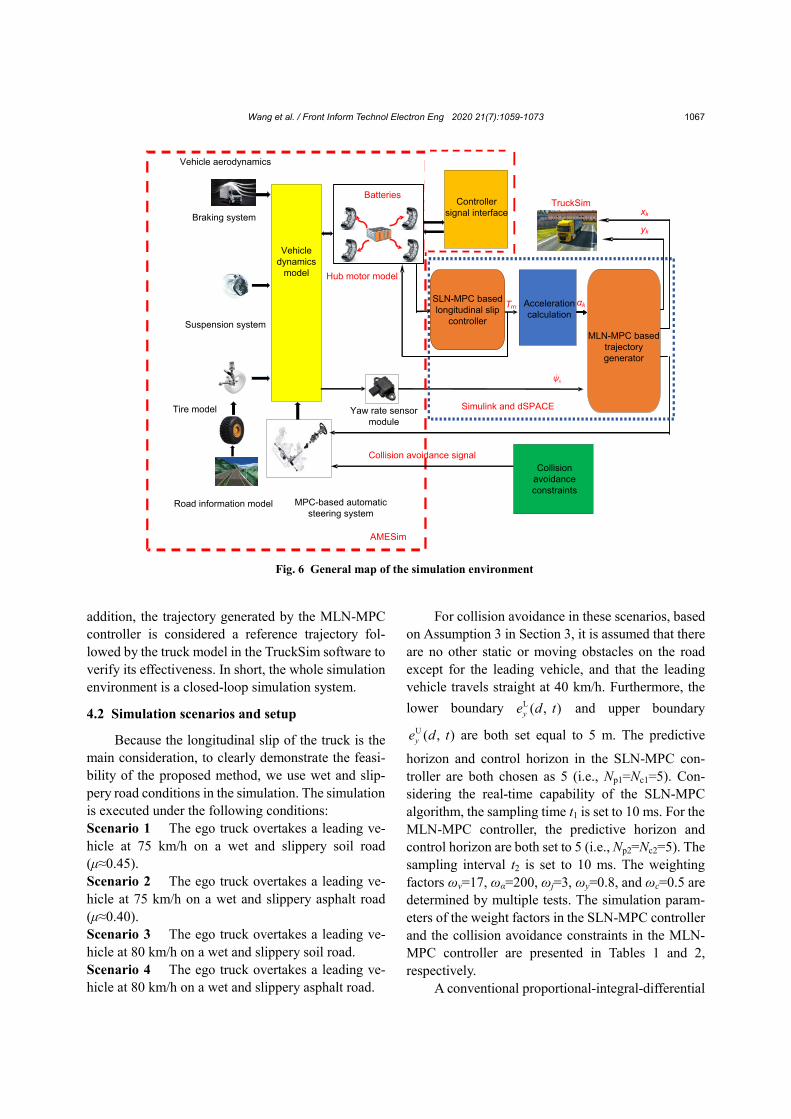
In this subsection, the effectiveness of the pro-posed control algorithm is verified in an off-line co-simulation environment, consisting of AMESim, Simulink, TruckSim, and dSPACE (rapid control prototyping). The general map of the simulation en-vironment is presented in Fig. 6. In the AMESim

system, to make the vehicle dynamics model more like a real vehicle, fully integrated sub-models are built, including vehicle aerodynamics, a braking system, a suspension system, a tire model, road in formation, and a steering system model.

The Simulink simulation environment includes mainly an SLN-MPC based longitudinal slip con-troller, a calculation model for acceleration, and an MLN-MPC based trajectory generator. To solve the nonlinear optimization function of constraints (14) and (15) in the SLN-MPC controller, the optimized routine e04wd is used. This routine is one of the solvers in the Numerical Algorithms Group (NAG) toolbox, and its function is to solve the sequence quadratic program (SQP) problem. In this study, the nonlinear optimization function of constraints (14) and (15) is implemented by the SQP method in this solver. Furthermore, the MLN-MPC problem in Eqs. (29)–(31) is solved with the Ipopt nonlinear programming solver via the YALMIP toolbox in Simulink. Because the YALMIP toolbox can solve several problems such as linear programming (LP), quadratic programming (QP), and second-order cone programming (SOCP), this problem (Eqs. (29)–(31)) can be solved by converting it into a QP problem. In

Fig. 4 MLN-MPC block diagram

MLN-MPC based trajectory generator

Calculate αk and αy,k

αmin≤αk≤αmax

Convex optimization cost function

min JFL(X(k), U(k))

αk

xk

yk

Ψk

vk

kψ

−αy,max≤αy,k≤αy,max

max maxkψ ψ ψ− ≤ ≤

Fig. 5 Implementation flowchart of the double-layer non-linear MPC problem

Initialization

Obtain measured values y(k)/y(t) and set the

reference output sequence r(k+j)/r(t)

Obtain the state estimated values x(k)/x(t)

Solve the sequence quadratic program (SQP)

problem

Solve the differential equations

If the SQP has a feasible solution

U*(k)/U*(t)?

Failure to control and

process separately

No

Apply these control variablesto the system

Yes

+( | ) / ( )k j k tu u

+( | ) / ( )k j k tu x+( | ) / ( )k j k tu y

= *( ) [1, 0, , 0] ( )k U ku

= *( ) [1, 0, ,0] ( )t U tu


addition, the trajectory generated by the MLN-MPC controller is considered a reference trajectory fol-lowed by the truck model in the TruckSim software to verify its effectiveness. In short, the whole simulation environment is a closed-loop simulation system.

4.2 Simulation scenarios and setup

Because the longitudinal slip of the truck is the main consideration, to clearly demonstrate the feasi-bility of the proposed method, we use wet and slip-pery road conditions in the simulation. The simulation is executed under the following conditions: Scenario 1 The ego truck overtakes a leading ve-hicle at 75 km/h on a wet and slippery soil road (μ≈0.45). Scenario 2 The ego truck overtakes a leading ve-hicle at 75 km/h on a wet and slippery asphalt road (μ≈0.40). Scenario 3 The ego truck overtakes a leading ve-hicle at 80 km/h on a wet and slippery soil road. Scenario 4 The ego truck overtakes a leading ve-hicle at 80 km/h on a wet and slippery asphalt road.

For collision avoidance in these scenarios, based on Assumption 3 in Section 3, it is assumed that there are no other static or moving obstacles on the road except for the leading vehicle, and that the leading vehicle travels straight at 40 km/h. Furthermore, the lower boundary L ( , )ye d t and upper boundary

U ( , )ye d t are both set equal to 5 m. The predictive

horizon and control horizon in the SLN-MPC con-troller are both chosen as 5 (i.e., Np1=Nc1=5). Con-sidering the real-time capability of the SLN-MPC algorithm, the sampling time t1 is set to 10 ms. For the MLN-MPC controller, the predictive horizon and control horizon are both set to 5 (i.e., Np2=Nc2=5). The sampling interval t2 is set to 10 ms. The weighting factors ων=17, ωα=200, ωj=3, ωy=0.8, and ωc=0.5 are determined by multiple tests. The simulation param-eters of the weight factors in the SLN-MPC controller and the collision avoidance constraints in the MLN- MPC controller are presented in Tables 1 and 2, respectively.

A conventional proportional-integral-differential

Fig. 6 General map of the simulation environment

TruckSim

Simulink and dSPACE

Vehicledynamics

model

Vehicle aerodynamics

Braking system

Suspension system

Tire model

Road information model

Batteries

Hub motor model

MPC-based automatic steering system

AMESim

Collision avoidance signal

Yaw rate sensor module

Controller signal interface

Collision avoidance constraints

Acceleration calculation

MLN-MPC based trajectory generator

SLN-MPC based longitudinal slip

controller

Tm αk

kψ

xk

yk


(PID) based control algorithm is executed to control the longitudinal slip within a stable zone to obtain contrasting simulation results. Simulation parameter settings and the road surface conditions in different scenarios are consistent with those of the proposed SLN-MPC based control algorithm, so that rationality in the comparison of the simulation can be ensured.

4.3 Simulation results and discussion

Fig. 7 indicates the trajectories generated by the MLN-MPC controller in different simulation sce-narios. Here, the red fields indicate the obstacles, including the lane boundaries and the leading vehicle. Assuming that there is only one obstacle vehicle, these three red boxes denote the positions of the ob-stacle vehicle at three simulation moments. The black dotted line is the road centerline, and these curves represent the trajectories generated by the MLN-MPC controller under four different simulation conditions.

In these simulation scenarios, to present the real- time position relationship between the ego vehicle and the obstacle vehicle during overtaking maneuver, the corresponding positions of the two vehicles at time instants t1–t6 have been marked. It can be seen from Figs. 8–11 that the ego vehicle can safely and

quickly overtake the obstacle vehicle, because the initial speed of the ego vehicle is greater than that of the obstacle vehicle. Furthermore, it can be concluded that the ego truck running with a higher initial speed starts earlier to execute a lane change than the ego truck running with a lower initial speed. However, for the truck running with a higher initial speed, it is time to return to the original lane after overtaking. Simi-larly, when the initial speed of the ego truck is invar-iable, the ego truck in the better road conditions starts earlier to execute lane change than the ego truck on the worse road conditions and returns to the original lane later after overtaking.

Table 1 Simulation parameters of weight factors in the SLN-MPC controller

Weight factor Value Q1 0.30 Q2 0.78 Q3 0.97 Q4 0.12 S1 0.04 S2 0.66 S3 0.93 S4 0.52

Table 2 Simulation parameters of collision avoidance constraints

Collision avoidance constraint Value

αmin 0 αmax 3.5 m/s2

maxψ 0.7 rad/s2 vmin 0 vmax 40 m/s

0 50 100 150 200x (m)

0−2−4−6

246

y (m

)

Obstacle

Lane boundaryPlanned trajectory on wet and slippery soil road at 75 km/hPlanned trajectory on wet and slippery asphalt road at 75 km/hPlanned trajectory on wet and slippery soil road at 80 km/hPlanned trajectory on wet and slippery asphalt road at 80 km/h

Road centerline

Fig. 7 Generated trajectories under different initial speeds and road conditions References to color refer to the online version of this figure

0−2−4−6

246

y (m

)

0 50 100 150 200x (m)

t1 t2

t3 t4

t5t6t1 t2 t3 t4 t5t6

Obstacle Ego truck

Lane boundaryRoad centerlinePlanned trajectory on wet and slippery soil road at 75 km/h

Fig. 8 Positions of the ego truck with an initial speed of 75 km/h and the leading vehicle moving at 40 km/h at time instants t1–t6 on a wet and slippery soil road

0−2−4−6

246

y (m

)

0 50 100 150 200x (m)

t1 t2

t3 t4

t5t6

t1 t2 t3 t4t5

t6

Obstacle Ego truck

Lane boundaryRoad centerlinePlanned trajectory on wet and slippery asphalt road at 75 km/h

Fig. 9 Positions of the ego truck with an initial speed of 75 km/h and the leading vehicle moving at 40 km/h at time instants t1–t6 on a wet and slippery asphalt road


To present the relative distance between the two

vehicles in these scenarios, the real-time trends of the relative distance from the simulation results are shown in Fig. 12. A denotes the relative distance between the points at which the ego truck starts lane change in these four scenarios. B indicates the relative distance between the points where the ego truck ends the initial lane change. C presents the relative distance between the points where the ego truck overtakes the leading vehicle. D shows the relative distance be-tween the points where the ego truck starts returning to the original lane. E denotes the relative distance between the points where the ego truck returns to the original lane. It can be seen from Fig. 12 that the time to reach the critical points (A, B, C, D, and E) of the vehicle in Scenario 1 is always the earliest. However, the time to reach these critical points in Scenario 4 is always the latest. This phenomenon can be explained by the fact that the ego truck in Scenario 1 has a lower initial speed and the road condition is poorer. It can also be known from Fig. 12 that the smallest relative distance is approximately 5 m, and that this distance can satisfy a safe distance in an overtaking maneuver in the real world.

Because the longitudinal slip of the wheels is used as a system constraint in the proposed algorithm,

the longitudinal slip during overtaking is tested in this simulation to further verify the feasibility of this method. The simulation results are presented in Figs. 13–16. To distinguish the longitudinal slip gen-erated by the SLN-MPC controller from the slip generated by the conventional PID-based control algorithm, ki-MPC and ki-PID are used to present their slip values, separately. When the ego truck starts to travel, the slip ki (i=fl-MPC, fr-MPC, rl-MPC, rr-MPC) increases dramatically because of the large driving torque generated by the motor. However, the stability of the truck is not jeopardized due to the role of cost functions JSL1 and JSL2. Note that there are two significant increases near 3.5 and 7.5 s in the entire simulation. This phenomenon is caused by the fact that the ego truck performs lane change before over-taking and returns to the original lane after overtaking during these two periods. However, it can be seen from the peaks of these two periods that no maximum longitudinal slip ratio exceeds 0.05 (within the stable zone). In addition, from Figs. 13–16, it can be sum-marized that there is a largest and a smallest longitu-dinal slip rate of the ego truck in Scenario 3 (Fig. 15) and Scenario 2 (Fig. 14), respectively. This is because there is a higher initial speed of the truck and a poorer road condition in Scenario 3, whereas in Scenario 2, there is a lower initial speed and a better road condition.

For the results of comparative simulation with the PID-based method, when the ego truck starts to travel, the slip ki (i=fl-PID, fr-PID, rl-PID, rr-PID) increases rapidly and significantly, exceeding the

0−2−4−6

246

y (m

)

0 50x (m)100 150 200

t1 t2

t3t4

t5t6

t1 t2 t3 t4t5

t6

Obstacle Ego truck

Lane boundaryRoad centerlinePlanned trajectory on wet and slippery soil road at 80 km/h

Fig. 10 Positions of the ego truck with an initial speed of 80 km/h and the leading vehicle moving at 40 km/h at time instants t1–t6 on a wet and slippery soil road

0−2−4−6

246

y (m

)

t1

t2t3

t4

t5t6

t1 t2 t3 t4 t5t6

0 50 100 150 200x (m)

Obstacle Ego truck

Lane boundaryRoad centerlinePlanned trajectory on wet and slippery asphalt road at 80 km/h

Fig. 11 Positions of the ego truck with an initial speed of 80 km/h and the leading vehicle moving at 40 km/h at time instants t1–t6 on a wet and slippery asphalt road

Fig. 12 Relative distance trends between the ego truck and the leading vehicle in the overtaking maneuver Relative distance corresponding to starting the lane change (A), ending the lane change (B), overtaking the leading vehicle (C), starting returning the original lane (D), and ending the return (E)

B

C

D

EA

Scenario 3 Scenario 4

60

0

10

20

30

50

40

0 1 2 3 4 5 6 7 8 9 10t (s)

Rel

ativ

e di

stan

ce (m

)

Scenario 1 Scenario 2


desired slip zone at t=1 s. Like the trends of ki-MPC, there are two large increases near t=3 and t=7 s in the four simulation scenarios. This is caused by the fact that the ego truck performs lane change before

overtaking and returns to the original lane after overtaking during the two periods. Furthermore, the change in ki-PID has a larger fluctuation than the change in ki-MPC in the whole simulation because of error compensation in the PID-based method.

To verify the computational cost of these meth-ods, the computational time in simulation is presented in Fig. 17. The orange and red areas denote the elapsed time to control the longitudinal slip by the PID-based (t=1.437 s) and SLN-MPC algorithms (t=0.821 s), respectively. The green and purple fields indicate the total time to control the longitudinal slip and generated trajectories by the PID+MLN-MPC (t=1.753 s) and SLN-MPC+MLN-MPC (t=1.137 s) algorithms, respectively. It can be concluded that the proposed algorithm SLN-MPC+MLN-MPC requires less time and is more efficient.

This method should provide the truck with a safe driving guarantee based on its safe driving

Fig. 17 Comparison of the elapsed time for the two algorithms References to color refer to the online version of this figure

1.437

1.753

0.821

PID PID+MLN-MPC

SLN-MPC SLN-MPC+MLN-MPC

Met

hod

Elapsed time (s)0 0.2 0.4 0.6 0.8 1.0 1.2 1.4 1.6 1.8

1.137

Fig. 13 Ego truck slip rate with the initial speed of 75 km/h during overtaking on a wet and slippery soil road

0 1 2 3 4 5 6 7 8 90

0.01

0.02

0.03

0.04

0.05

0.06

0.07

Slip

rate

t (s)

krr-MPCkrl-MPC

krr-PIDkrl-PIDkfl-PID kfr-PID

kfl-MPC kfr-MPC

Fig. 14 Ego truck slip rate with the initial speed of 75 km/h during overtaking on a wet and slippery asphalt road

0 1 2 3 4 5 6 7 8 90

0.01

0.02

0.03

0.04

0.05

0.06

0.07

Slip

rate

t (s)

krr-MPCkrl-MPC


kfl-MPC kfr-MPC

Fig. 15 Ego truck slip rate with the initial speed of 80 km/h during overtaking on a wet and slippery soil road

0 1 2 3 4 5 6 7 8 90

0.01

0.02

0.03

0.04

0.05

0.06

0.07

Slip

rate

t (s)

krr-MPCkrl-MPC


kfl-MPC kfr-MPC

Fig. 16 Ego truck slip rate with the initial speed of 80 km/h during overtaking on a wet and slippery asphalt road

0 1 2 3 4 5 6 7 8 90

0.01

0.02

0.03

0.04

0.05

0.06

0.07

Slip

rate

t (s)

krr-MPCkrl-MPC


kfl-MPC kfr-MPC


requirements. Here, the lateral acceleration of the truck during overtaking maneuver should be limited to a safe range. Therefore, in this simulation, the lat-eral acceleration trend is verified in four simulation scenarios. It can be seen from Fig. 18 that the lateral acceleration of the truck does not exceed the safety threshold (αy<0.4g, g is the gravity acceleration) during the lane change. Based on all the simulation results above, the proposed method can accurately control the longitudinal slip within a stable zone and satisfy the safety requirements of the truck during overtaking.

In addition, because the hub motor torque in this

model is constrained by the maximum output torque and the optimal longitudinal slip, the motor torque is usually maintained within a smooth working range, but the optimal longitudinal slip may not be achieved in some extreme driving conditions. Therefore, we verify that the proposed algorithm is feasible for ap-plications in the real world or future research. A driver model is shown in Fig. 19, which provides an external signal input of the motor torque. This model is con-nected to the simulation system to verify the stability and robustness of the control algorithm when the motor torque is determined by driver’s behaviors. Sub-modules under the AMESim environment are not changed. In this test, two drivers provide the signal input of the motor torque based on the accelerator pedal action; the trends are shown in Fig. 20. Note that other pedals in the equipment have no signal input. Test results with these inputs are shown in Fig. 21.

Overall, it can be seen from Fig. 21 that the ki-driver j (i=fl, fr, rl, rr, j=1, 2) generated by these two

drivers’ behaviors is changed with pedal’s opening. Furthermore, under the two extreme test conditions at 1.83 and 4.51 s, the maximum slip values of ki-driver 1 and ki-driver 2 are 0.042 and 0.039, respectively. The fluctuation of slip ki-driver j can be kept within a desired range (0–0.05) during the whole test. Therefore, we conclude that the control algorithm can protect the truck against external irregular disturbances from humans or environments.

On wet slippery soil road at 80 km/hOn wet slippery asphalt road at 75 km/hOn wet slippery soil road at 75 km/h

On wet slippery asphalt road at 80 km/h

4

0

−2

−4−3

23

Late

ral a

ccel

erat

ion

(m/s

2 )

1

−1

0 1 2 3 4 5 6 7 8t (s)

9

Fig. 18 Lateral acceleration changes of the truck during the overtaking maneuver

Fig. 20 Trends of the accelerator pedal controlled by drivers

Driver 1Driver 2

0 1 2 3 4 5 6 7 8t (s)

90

10

20

30

40

50

60

Ped

al a

ngle

(°)

Fig. 21 Ego truck slip rate produced by the driver model

0 1 2 3 4 5 6 7 8t (s)

90

0.01

0.02

0.03

0.04

0.05

Slip

rate

krr-driver 1krl-driver 1kfl-driver 1 kfr-driver 1

krr-driver 2krl-driver 2kfl-driver 2 kfr-driver 2

Fig. 19 Test platform of the driver model


5 Conclusions

A double-layered control algorithm has been developed to plan the local trajectory for autonomous trucks equipped with four hub motors. The results showed that this proposed algorithm makes it possible to generate a dynamically feasible and customizable trajectory. The longitudinal wheel slip controlled by the SLN-MPC controller in uncertain road conditions can be accurately controlled within a stable zone. This slip had a smaller maximum and smoother fluctuation than that of the conventional PID-based control method. In overtaking maneuver, the lateral acceler-ation of the truck is limited to a safety range to avoid truck side slipping. Thus, the ego truck can complete overtaking maneuver safely under the formulated avoidance constraints. Co-simulation results showed that this method guarantees that the truck will operate safely, satisfy its driving requirements, and provide a feasible reference basis for applications in the real world.

There are still some issues that need to be ex-plored in the future. On the one hand, the collision avoidance system in this study needs to be improved, because it is assumed that there is only one leading obstacle vehicle and no other static or moving obsta-cle around the ego truck. On the other hand, to verify the real-time performance, a hardware-in-the-loop simulation (HILS) needs to be developed in the pro-posed double-layered nonlinear MPC controller. High-efficiency energy-saving measures in practical commercial motor applications need to be further studied. Contributors

Hong-chao WANG designed the research. Hong-chao WANG, Wei-wei ZHANG, Hao-tian CAO, and Xun-cheng WU designed the algorithms and processed the data. Hong-chao WANG, Wei-wei ZHANG, Qiao-ming GAO, and Su-yun LUO drafted the manuscript. Hong-chao WANG and Wei-wei ZHANG revised and finalized the paper. Compliance with ethics guidelines

Hong-chao WANG, Wei-wei ZHANG, Xun-cheng WU, Hao-tian CAO, Qiao-ming GAO, and Su-yun LUO declare that they have no conflict of interest. References Amodeo M, Ferrara A, Terzaghi R, et al., 2010. Wheel slip

control via second-order sliding-mode generation. IEEE

Trans Intell Transp Syst, 11(1):122-131. https://doi.org/10.1109/TITS.2009.2035438

Anderson SJ, Peters SC, Pilutti TE, et al., 2010. An optimal- control-based framework for trajectory planning, threat assessment, and semi-autonomous control of passenger vehicles in hazard avoidance scenarios. Int J Veh Auton Syst, 8(2-4):190-216.

https://doi.org/10.1504/IJVAS.2010.035796 Barraquand J, Langlois B, Latombe JC, 1992. Numerical

potential field techniques for robot path planning. IEEE Trans Syst Man Cybern, 22(2):224-241.

https://doi.org/10.1109/21.148426 Borenstein J, Koren Y, 1991. The vector field histogram—fast

obstacle avoidance for mobile robots. IEEE Trans Robot Autom, 7(3):278-288. https://doi.org/10.1109/70.88137

Carvalho A, Gao YQ, Gray A, et al., 2013. Predictive control of an autonomous ground vehicle using an iterative line-arization approach. Proc 16th Int IEEE Conf on Intelligent Transportation Systems, p.2335-2340.

https://doi.org/10.1109/ITSC.2013.6728576 Cesari G, Schildbach G, Carvalho A, et al., 2017. Scenario

model predictive control for lane change assistance and autonomous driving on highways. IEEE Intell Trans Syst Mag, 9(3):23-35. https://doi.org/10.1109/MITS.2017.2709782

Chen H, 2013. Model Predictive Control. Science Press, Bei-jing, China (in Chinese).

Chu K, Lee M, Sunwoo M, 2012. Local path planning for off- road autonomous driving with avoidance of static obsta-cles. IEEE Trans Intell Trans Syst, 13(4):1599-1616.

https://doi.org/10.1109/TITS.2012.2198214 de Castro R, Araújo RE, Tanelli M, et al., 2012. Torque

blending and wheel slip control in EVs with in-wheel motors. Veh Syst Dynam, 20(1):71-94.

https://doi.org/10.1080/00423114.2012.666357 de Castro R, Araújo RE, Freitas D, 2013. Wheel slip control of

EVs based on sliding mode technique with conditional integrators. IEEE Trans Ind Electron, 60(8):3256-3271. https://doi.org/10.1109/TIE.2012.2202357

Dixit S, Fallah S, Montanaro U, et al., 2018. Trajectory plan-ning and tracking for autonomous overtaking: state-of- the-art and future prospects. Ann Rev Contr, 45:76-86.

https://doi.org/10.1016/j.arcontrol.2018.02.001 Gao Y, Gray A, Frasch J, et al., 2012. Spatial predictive control

for agile semi-autonomous ground vehicles. Proc 11th Int Symp on Advanced Vehicle Control, p.1-6.

Gao YQ, Gray A, Tseng HE, et al., 2014. A tube-based robust nonlinear predictive control approach to semiautonomous ground vehicles. Veh Syst Dynam, 52(6):802-823.

https://doi.org/10.1080/00423114.2014.902537 Glaser S, Vanholme B, Mammar S, et al., 2010. Maneuver-

based trajectory planning for highly autonomous vehicles on real road with traffic and driver interaction. IEEE Trans Intell Trans Syst, 11(3):589-606. https://doi.org/10.1109/TITS.2010.2046037

Katrakazas C, Quddus M, Chen WH, et al., 2015. Real-time


motion planning methods for autonomous on-road driv-ing: state-of-the-art and future research directions. Trans Res Part C, 60:416-442. https://doi.org/10.1016/j.trc.2015.09.011

Kim B, Kim D, Park S, et al., 2016. Automated complex urban driving based on enhanced environment representation with GPS/map, radar, lidar and vision. IFAC- PapersOnLine, 49(11):190-195. https://doi.org/10.1016/j.ifacol.2016.08.029

Kim J, Lee J, 2018. Traction-energy balancing adaptive control with slip optimization for wheeled robots on rough terrain. Cogn Syst Res, 49:142-156.

https://doi.org/10.1016/j.cogsys.2018.01.007 Kitazawa S, Kaneko T, 2017. Control target algorithm for

direction control of autonomous vehicles in consideration of mutual accordance in mixed traffic conditions. Int Symp on Advanced Vehicle Control, p.151-156.

Lanza G, Ferdows K, Kara S, et al., 2019. Global production networks: design and operation. CIRP Ann, 68:823-841.

https://doi.org/10.1016/j.cirp.2019.05.008 Laskaris KI, Kladas AG, 2010. Internal permanent magnet

motor design for electric vehicle drive. IEEE Trans Ind Electron, 57(1):138-145.

https://doi.org/10.1109/TIE.2009.2033086 Li SH, Yang SP, 2015. Investigation on dynamics of a three-

directional coupled vehicle-road system. J Vibroeng, 17(7):3887-3908.

Ma L, Xue JR, Kawabata K, et al., 2014. A fast RRT algorithm for motion planning of autonomous road vehicles. Proc 17th Int IEEE Conf on Intelligent Transportation Systems, p.1033-1038. https://doi.org/10.1109/ITSC.2014.6957824

Mareev I, Becker J, Sauer DU, 2018. Battery dimensioning and life cycle costs analysis for a heavy-duty truck con-sidering the requirements of long-haul transportation. Energies, 11(1):55. https://doi.org/10.3390/en11010055

Mittal N, Udayakumar PD, Raghuram G, et al., 2018. The endemic issue of truck driver shortage—a comparative study between India and the United States. Res Trans Econ, 71:76-84. https://doi.org/10.1016/j.retrec.2018.06.005

Mutoh N, 2012. Driving and braking torque distribution methods for front- and rear-wheel-independent drive-type electric vehicles on roads with low friction coefficient. IEEE Trans Ind Electron, 59(10):3919-3933.

https://doi.org/10.1109/TIE.2012.2186772 Nilsson J, Gao YQ, Carvalho A, et al., 2014. Manoeuvre gen-

eration and control for automated highway driving. IFAC Proc Vol, 47(3):6301-6306.

https://doi.org/10.3182/20140824-6-ZA-1003.00619 Shamir T, 2004. How should an autonomous vehicle overtake a

slower moving vehicle: design and analysis of an optimal trajectory. IEEE Trans Autom Contr, 49(4):607-610.

https://doi.org/10.1109/TAC.2004.825632 Shim T, Adireddy G, Yuan HL, 2012. Autonomous vehicle

collision avoidance system using path planning and model-predictive-control-based active front steering and wheel torque control. Proc Inst Mech Eng Part D, 226(6): 767-778. https://doi.org/10.1177/0954407011430275

So J, Park B, Wolfe SM, et al., 2014. Development and vali-dation of a vehicle dynamics integrated traffic simulation environment assessing surrogate safety. J Comput Civ Eng, 29(5):04014080.

https://doi.org/10.1061/(ASCE)CP.1943-5487.0000403

Documents

A double-layered nonlinear model predictive control based