A Double Homotopy Approach for Decentralized ∞ Control of Civil Structures

Chunxu Qu 1,2

, Linsheng Huo 1,,†

, Hongnan Li 1, Yang Wang

2

1 Faculty of Infrastructure Engineering, Dalian University of Technology, Dalian 116024,

China 2 School of Civil and Environmental Engineering, Georgia Institute of Technology,

Atlanta, GA 30332, USA

ABSTRACT

This paper presents a decentralized ∞ controller design for the vibration control of

civil structures. The formulation through double homotopy is proposed in discrete time

domain and considers feedback time delay. It is well known that through bounded real

lemma, ∞ controller design can be transformed to an optimization problem with bilinear

matrix inequality (BMI) constraints. To obtain a decentralized ∞ controller constrained

by special block-diagonal patterns on controller matrices, there is generally no off-the-

shelf package or numerical algorithm to solve the BMI problem. This paper proposes a

double homotopy method to solve the BMI problem in discrete time domain. The method

approximates the BMI problem to a series of linear matrix inequality (LMI) problems

along two homotopic paths, and gradually deforms a centralized controller to a

decentralized controller. The proposed method is first studied numerically with a six-

story building example, and then validated experimentally through shaking table tests of

a two-story frame with active mass dampers.

KEY WORDS: structural control; decentralized control; bilinear matrix inequality;

double homotopy; time delay; civil structures

INTRODUCTION

Excessive dynamic excitations upon civil structures, such as earthquakes and wind

load, can cause significant structural vibrations and result in damage to structural

components. Structural control is a promising method to protect structures from damage.

A great amount of research efforts have been devoted to active or semi-active feedback

control [1-4]. Such a feedback control system contains sensors, controllers, and control

devices. Sensors measure structural vibration data caused by external excitations. Sensor

data is then transmitted to controllers, which make control decisions accordingly, and

command the control devices to generate desired forces for vibration reduction.

Traditional structural feedback control adopts centralized control schemes, where a

centralized controller requires data from all sensors in the structure and delivers

Correspondence to: Linsheng Huo, of Infrastructure Engineering, Dalian University of Technology,

Dalian 116024, China.

†E-mail: lshuo@dlut.edu.cn

command to all structural control devices. Particularly for large-scale civil structures, a

centralized feedback control scheme places high requirements on real-time

communication range and data transmission rate, which result in economical and

technical difficulties in practical implementation.

As an alternative, decentralized control architectures can be employed. A

decentralized architecture allows control decisions to be made using sensor data only in

the neighborhood of a control device [5, 6]. As a result, communication range and data

transmission rate are reduced. Feedback latency of the control system is also shortened.

Decentralized control has been investigated in applications such as power transmission

networks, economic systems, and space systems [7]. However, decentralized structural

control has only been studied in recent years. For example, Lynch and Law [8] discussed

modified decentralized LQR control and decentralized market-based control for large-

scale civil structures. Xu et al. [9] proposed a decentralized tendon control algorithm for

a cable-stayed bridge with neural networks. Swartz and Lynch [10] employed the

redundant Kalman state-estimators for distributed structural control system. Rofooei and

S.Monajemi-Nezhad [11] investigated decentralized schemes in which instantaneous

optimal control schemes are used with different control feedbacks. Lu et al. [12]

described the fully decentralized sliding mode control algorithms, which make control

decision based on the stroke velocity and displacement measured on a control device. Ma

et al. [13] studied decentralized robust control of building structures by treating the

interconnections between adjacent subsystems as bounded disturbances. Loh and Chang

[14] compared four groups of centralized/decentralized control algorithms, including

fully centralized, fully decentralized, half centralized, and partially decentralized control.

More recently, feedback time delay, such as due to communication and computing, is

taken into consideration for decentralized dynamic output feedback control [15, 16]. In

general, the more sensor data each control device requires, the larger the time delay is.

Time delay can be measured and calculated as part of the system performance, such as

for a wireless feedback control system [17]. Considering feedback time delay in the

control formulation, this paper presented a new ∞ structural control design for

decentralized dynamic output feedback control in discrete time domain.

Bounded real lemma [18] can be used to provide an effective method to calculate

the ∞ controller matrices. The controller matrices are constrained by bilinear matrix

inequality (BMI) [19]. When no special patterns are required on controller matrices, the

matrices can be solved by projection lemma [18]. On the other hand, when a

decentralized controller is desired, block-diagonal patterns are required on the controller

matrices. The pattern requirement makes the decentralized controller design a non-

convex and NP-hard problem. There is no general off-the-shelf package or numerical

algorithm for this decentralized control problem. For example, when the PENNON

(PENalty methods for NONlinear optimization) package was attempted for solving non-

convex optimization problems, it was realized the idea was not yet mature and further

tuning was needed [20]. Wang [16] modified a continuous-time homotopy method for

discrete-time decentralized ∞ controller design with feedback time delay. Along the

homotopy path, the centralized controller is gradually transformed to a decentralized

controller. Only linear matrix inequality (LMI) problems are involved at each homotopy

step, which avoids directly solving the BMI problem. As an alternative method to deal

with BMI constraints, Mehendale and Grigoriadis [21] proposed a double homotopy

approach for decentralized ∞ control in continuous time domain without time delay.

This paper modifies the double homotopy method for decentralized control design in

discrete time domain and considering feedback time delay. Along one homotopy path,

the centralized controller is slowly deformed to a decentralized controller. Along the

other homotopy path, the solution to the BMI problem is gradually improved by local

linearization. In a previous discrete-time homotopy approach described by Wang [16], at

every homotopy step, the controller matrix or the Lyapunov matrix is held constant in

turn while solving the other. In comparison, the double homotopy approach updates the

controller matrix and Lyapunov matrix simultaneously by local linearization to the

original BMI problem. In addition, minimization of closed-loop ∞ norm is performed

at every double homotopy step, in order to avoid resulting in a decentralized controller

with a very large ∞ norm. Both numerical simulations and laboratory experiments

were performed to validate the proposed discrete-time decentralized control design

through double homotopy.

The paper first introduces the problem formulation for decentralized structural

control considering time delay. The decentralized ∞ control through double homotopy

transformation in discrete time domain is then presented. A six-story numerical example

is described to illustrate the decentralized ∞ control performance. Finally, the paper

describes experimental validation through shaking table tests of a two-story frame with

active mass dampers.

PROBLEM FORMULATION

Consider a second-order differential equation describing the dynamics of an n

degree-of-freedom (DOF) shear-frame structure:

1 1w uMq Cq Kq T w T u (1)

where , , n nM C K are the mass, damping, and stiffness matrices, respectively; 1 1

1wn

w

is the external excitation vector; 1unu

is the control force vector; Tw1 and

Tu are the location matrices for excitation w1 and control force u, respectively. When the

excitation w1 is the unidirectional earthquake acceleration gq , the excitation location

matrix can be found as 1 1{1}w nT M . The relative displacement vector q1n is

defined as:

T

1 2 nq q q q (2)

where qi denotes the relative displacement (with respect to the ground) of the i-th floor.

To suppress excessive structural vibration excited by w1, appropriate control force u

should be imposed on the structure. In an optimal feedback control system, a controller is

pre-designed. During system operation, according to available sensor measurements, the

controller decides in real time the optimal control force to be applied by each control

device. In practice, sensor measurements are usually contaminated by noises. In addition,

transmission of measurement data to controller, as well as controller computation, causes

time delay in the feedback loop.

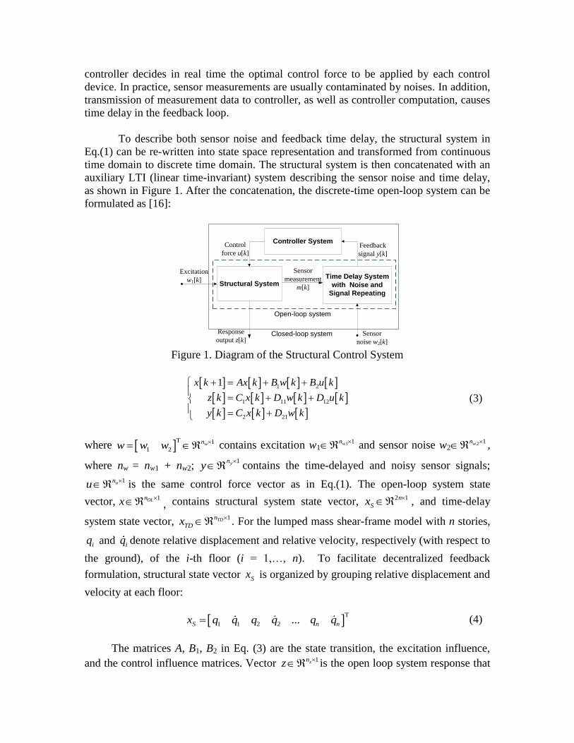
To describe both sensor noise and feedback time delay, the structural system in

Eq.(1) can be re-written into state space representation and transformed from continuous

time domain to discrete time domain. The structural system is then concatenated with an

auxiliary LTI (linear time-invariant) system describing the sensor noise and time delay,

as shown in Figure 1. After the concatenation, the discrete-time open-loop system can be

formulated as [16]:

Excitation

w1[k]

Response

output z[k]

Sensor

measurement

m[k]

Time Delay System

with Noise and

Signal Repeating

Sensor

noise w2[k]

Controller SystemFeedback

signal y[k]

Control

force u[k]

Open-loop system

Closed-loop system

Structural System

Figure 1. Diagram of the Structural Control System

1 2

1 11 12

2 21

1x k Ax k B w k B u k

z k C x k D w k D u k

y k C x k D w k

(3)

where T 1

1 2wn

w w w

contains excitation w11 1wn

and sensor noise w22 1wn

,

where nw = nw1 + nw2; 1yn

y

contains the time-delayed and noisy sensor signals;

1unu

is the same control force vector as in Eq.(1). The open-loop system state

vector, 1OLnx

, contains structural system state vector,

2 1n

Sx , and time-delay

system state vector, 1TDn

TDx . For the lumped mass shear-frame model with n stories,

iq and iq denote relative displacement and relative velocity, respectively (with respect to

the ground), of the i-th floor (i = 1,…, n). To facilitate decentralized feedback

formulation, structural state vector Sx is organized by grouping relative displacement and

velocity at each floor:

T

1 1 2 2 ...S n nx q q q q q q (4)

The matrices A, B1, B2 in Eq. (3) are the state transition, the excitation influence,

and the control influence matrices. Vector 1znz is the open loop system response that

the system aims to control, and 1yn

y

is the sensor measurement with time delay and

noise. To complete a feedback loop, vector y also serves as the input to the controller

system to be designed, which is described as:

1G G G G

G G G

x k A x k B y k

u k C x k D y k

(5)

where xG1Gn

is the controller state vector; AG, BG, CG, DG are constant matrices of the

LTI dynamic controller and are to be determined through an optimal control design.

DECENTRALIZED CONTROLLER DESIGN IN DISCRETE TIME THROUGH

DOUBLE HOMOTOPY APPROACH

Decentralized Controller Design

For decentralized controller design, the decentralization is represented through

block-diagonal patterns in the controller matrices:

1 2

1 2

1 2

1 2

diag , ,

diag , ,

diag , ,

diag , ,

N

N

N

N

G G G G

G G G G

G G G G

G G G G

A A A A

B B B B

C C C C

D D D D

(6)

With the block-diagonal patterns, the controller system in Eq. (5) is equivalent to

multiple sub-controllers that are independent from each other. Every sub-controller

needs only part of sensor measurement data as input and determines only part of the

control forces as output:

1 1 1 1

1 1 1

1

1 1

1

G G G G

G G G

x k A x k B y k

u k C x k D y k

…,

1i i i i

i i i

G G G G i

i G G G i

x k A x k B y k

u k C x k D y k

…,

1N N N N

N N N

G G G G N

N G G G N

x k A x k B y k

u k C x k D y k

(7)

where , , ,i i i iG G G GA B C D are matrices of the i-th sub-controller, i=1…N); yi is the sensor

measurement data required by the i-th sub-controller; ui is the control force determined

by the i-th sub-controller. As a result, the overall sensor measurement and control force

vectors are partitioned by sub-controllers:

T

1 i Ny y y y

(8a)

T

1 i Nu u u u

(8b)

For convenience in later derivation, the following notations should be defined first

based on parametric matrices of the open-loop system in Eq.(3):

1 2

1 2

1 11 12 1 11 12

2 21

2 21

0 0

0 0 0 0

0 0

0 0

0

G

G

n

n

A B B

IA B B

C D D C D D

C D I

C D

(9)

where nG is the order of decentralized controller. Combining the open-loop system and

the controller system in Eq. (5), the closed-loop system is formulated as:

1CL CL CL CL

CL CL CL

x k A x k B w k

z k C x k D w k

(10a)

2 2CLA A B GC

(10b)

1 2 21CLB B B GD

(10c)

1 12 2CLC C D GC

(10d)

11 12 21CLD D D GD

(10e)

where CLx is the state vector of the closed-loop system; G is the overall controller matrix

that contains all four parametric matrices in the controller system:

G G

G G

A BG

C D

(11)

An ∞ controller design aims to determine a proper controller matrix G so that ∞

norm of the closed-loop system is minimized. As a result, dynamic response of the

structural system is reduced. According to bounded real lemma in discrete time, an ∞

controller can be designed to make the closed-loop system stable and its ∞ norm smaller

than a given scalar γ, if and only if, there exists a symmetric positive definite matrix P >

0 such that the following matrix inequality holds:

T

T

0

* 00

* *

* * *

CL CL

CL

CL

P PA PB

P C

I D

I

(12)

where denotes the terms induced by symmetry. Substituting Eq.(10b) - (10e) into

Eq.(12), the matrix inequality now contains the controller matrix G and other constant

parametric matrices defined in Eq. (9):

2 2 1 2 21

T

1 12 2

T

11 12 21

0

* 00

* *

* * *

P P A B GC P B B GD

P C D GC

I D D GD

I

(13)

Linear Matrix Inequality and Bilinear Matrix Inequality

A linear matrix inequality (LMI) has the form as the following [19]:

0

1

0m

i i

i

F x F x F

(14)

where mx is the vector variable and the symmetric matrices T n n

i iF F , i =

0,…,m, are given. The inequality symbol in Eq.(14) means that F(x) is positive definite.

An important property of LMI is that the set | 0x F x is convex, which can serve as

constraint of a convex optimization problem. On the other hand, the bilinear matrix

inequality (BMI) is of the form:

0

1 1 1 1

, 0m n m n

i i j j i j ij

i j i j

F x y F x F y G x y H

(15)

where Gj and Hij are symmetric matrices, and mx and ny are vector variables. A

BMI is an LMI in x for fixed y, or an LMI in y for fixed x. However, the BMI constraint

doesn’t provide a convex set on x and y simultaneously.

Double Homotopy Approach

Eq. (13) has terms of matrix product that involves both unknown variables P and G,

which results in a bilinear matrix inequality (BMI). When there is no special pattern

requirement on G, such as in a traditional centralized controller design, the BMI problem

can be solved by projection lemma [18]. However, with a block-diagonal pattern

constraint to the matrix variable G, as required by a decentralized design, the problem

becomes NP-hard. There is no general off-the-shelf numerical package or algorithm for

such a non-convex decentralized control problem. For example, algorithm in the

PENNON package is modified for finding local minima or stationary points in a

nonconvex problem, but the idea is found to be not yet mature and needs further tuning

[20]. More recently, Mehendale and Grigoriadis [21] proposed a heuristic double

homotopy algorithm to solve the decentralized ∞ controller in continuous time domain.

In this paper, the double homotopy concept is adopted to design a decentralized ∞

controller in discrete time domain.

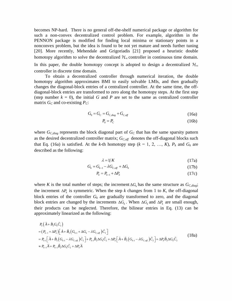
To obtain a decentralized controller through numerical iteration, the double

homotopy algorithm approximates BMI to easily solvable LMIs, and then gradually

changes the diagonal-block entries of a centralized controller. At the same time, the off-

diagonal-block entries are transformed to zero along the homotopy steps. At the first step

(step number k = 0), the initial G and P are set to the same as centralized controller

matrix GC and co-existing PC:

0 , ,C C diag C offG G G G (16a)

0 CP P

(16b)

where GC,diag represents the block diagonal part of GC that has the same sparsity pattern

as the desired decentralized controller matrix; GC,off denotes the off-diagonal blocks such

that Eq. (16a) is satisfied. At the k-th homotopy step (k = 1, 2, …, K), Pk and Gk are

described as the following:

1 K (17a)

1 ,k k C off kG G G G (17b)

1k k kP P P

(17c)

where K is the total number of steps; the increment kG has the same structure as GC,diag;

the increment kP is symmetric. When the step k changes from 1 to K, the off-diagonal

block entries of the controller Gk are gradually transformed to zero, and the diagonal

block entries are changed by the increments kG . When kG and kP are small enough,

their products can be neglected. Therefore, the bilinear entries in Eq. (13) can be

approximately linearized as the following:

2 2

1 2 -1 , 2

-1 2 -1 , 2 -1 2 2 2 -1 , 2 2 2

1 1 2 2

k k

k k k k C off

k k C off k k k k C off k k

k k k k

P A B G C

P P A B G G G C

P A B G G C P B G C P A B G G C P B G C

P A P B G C P A

(18a)

1 2 21

-1 1 2 -1 , 21

-1 1 2 -1 , 21 -1 2 21 1 2 -1 , 21 2 21

1 1 2 21

k k

k k k k C off

k k C off k k k k C off k k

k k k k

P B B G D

P P B B G G G D

P B B G G D P B G D P B B G G D P B G D

P B P B G D P B

(18b)

As a result, the BMI problem is converted to an LMI problem where there is no

matrix product simultaneously involving kG and

kP . Substituting Gk in Eq.(17b) into

other entries in Eq.(13), the following equation can be derived:

1 12 2 1 12 -1 , 2

1 12 -1 , 2 12 2

12 2

k k k C off

k C off k

k

C D G C C D G G G C

C D G G C D G C

C D G C

(19a)

11 12 21 11 12 -1 , 21

11 12 -1 , 21 12 21

12 21

k k k C off

k C off k

k

D D G D D D G G G D

D D G G D D G D

D D G D

(19b)

where

2 -1 , 2k C offA A B G G C (20a)

1 2 -1 , 21k C offB B B G G D

(20b)

1 12 -1 , 2k C offC C D G G C

(20c)

11 12 -1 , 21k C offD D D G G D

(20d)

Finally, the LMI after linearizing BMI in Eq. (13) can be re-written with variables

kG and kP :

1 1 1 2 2 1 1 2 21

1 12 2

12 21

,

0

* 00

* *

* * *

k k

k k k k k k k k k k

T

k k k

T

k

V G P

P P P A P B G C P A P B P B G D P B

P P C D G C

I D D G D

I

(21)

The double homotopy process for searching a decentralized controller is described

as below:

Step 1: Compute a centralized ∞ controller GC, as well as co-existing PC and γC, and

then separate GC,diag and GC,off according to Eq. (16a).

Step 2: Set the upper limit Kmax for K, e.g. 213

, and γmax for γ, e.g. 28γC. Initialize K, e.g.

26, k←1, P0←PC, G0 ←GC, γ0← γC.

Step 3: At step k, calculate the symmetric increment variable matrix kP , the structured

increment variable matrixkG , and scale variable γk in the following LMI problem.

Minimize γk

Subject to ,k kV G P <0, 1 0k kP P , 1k kP P , k CG G ,

1k k .

(22)

Step 4: Set Gk← 1 ,k C off kG G G and Pk← 1k kP P . Check that the triplet (Gk, Pk, γk)

satisfies the inequality Eq. (13). If they do, recalculate Pk by fixing Gk and γk in Eq.

(13) to improve the condition number of Pk, and then go to Step 5. If not, set K←2K.

If K<Kmax, repeat Step 3 with the initial value P0, G0, γ0; otherwise set γ0←2γC under

the constraint γ0 ≤ γmax, and go to Step 3 with the initial value P0, G0, K, k. If γ0

grows larger than the pre-set limit γmax, it is concluded that the algorithm does not

converge.

Step 5: If k = K, the desired decentralized ∞ controller is given by Gk. If not, set k←k+1,

and repeat Step 3 with the updated Pk, Gk, and γk.

It should be noted that this double homotopy method is heuristic and cannot

guarantee convergence. Even if the process converges, the solution may still be a local

optimum due to the non-convex nature of the decentralized control problem. On the

other hand, non-convergence does not imply the non-existence of a decentralized ∞

controller.

NUMERICAL EXAMPLE

This section studies performance comparison between the proposed decentralized

controller design and centralized design, using a six-story model structure. The six-story

structure is shown in Figure 2(a). Lumped mass parameters are provided in Figure 2(b)

and other parameters are described in [12]. Three ideal actuators are installed on the 1st,

3rd

and 5th

floor, respectively. Through a V-brace, every actuator can apply control force

between two neighboring floors.

(a) deployment of three

actuators

(b) lumped masses

of the structure

(c) communication architecture

for different DC

Figure 2. A six-story model structure centralization (DC)

The measurement output m[k] are denoted as the inter-story drifts described in Eq.

(23a). Sensor noise can influence the measurement results, and worsen the control

performance. In this simulation, the sensor noise level is set as 0.1% of the sensor signal.

Considering the time delay and sensor noise, the feedback signal y[k] is formed as in Eq.

(3). Eq. (23b) defines the response output z[k] as the combination of inter-story drifts and

control force with different weightings .

T

1 2 1 6 5m k q k q k q k q k q k (23a)

T

4 9

1 2 1 6 5 1 2 310 , 10z k q k q k q k q k q k u u u

(23b)

As shown in Figure 2(c), four different feedback cases are studied, representing

different degrees of centralization (DC). In each DC, there exist one or more

communication subnets (as denoted by channels Ch1, Ch2, etc). A larger number of DC

represents a higher level of centralization. For example, DC means each subnet or

channel covers only one story and there are three subnets totally. Each subnet in DC

covers two stories and a total of three subnets exist, without overlapping between two

channels. For case DC , each subnet covers four stories and the two communication

channels overlap at 3rd

and 4th

stories. For DC , only one subnet exists and covers all six

stories, representing centralized control.

In practical implementation, the sampling period for different control architecture is

determined by the network communication time and computation time of the embedded

controllers. For a particular control system, values of the time delays can be measured

according to sensor and controller deployment. As commonly encountered, the time

delay in this study equals one sampling time step, i.e. the time delay equals one sampling

period. Due to the least amount of communication and computation required, case

DC entails shortest sampling period and least time delay. A larger number of DC

usually indicates more time is required for communication and computation. Case DC

thus has the longest sampling period and time delay. Using a prototype wireless

feedback control system as an example [17], the sampling period and time delay from

DC to DC adopted in this simulation are displayed in Table 1.

Table 1. Feedback time delay and sampling period for four different DCs (unit: ms)

DC DC DC DC

15 20 25 52

The controllers for different DC cases are designed using the proposed double

homotopy method for discrete time domain. The 1940 El Centro NS earthquake record is

adopted as the ground excitation. The peak ground acceleration is scaled to 1 m/s2.

Classical Newmark integration is performed to compute time histories of structural

response during the earthquake. For all cases with control and without control, the

structure response is evaluated by peak inter-story drifts shown in Figure 3(a).

Theoretically, the system should still be stable for all cases, even with ideal actuators that

are capable of producing any desired forces. However, it is found that DC and DC

demonstrate unstable structural response in the Newmark integration, which means that

the marginally low stability of these two cases is easily disturbed in the numerical

integration. Figure 3(b) shows that due to instability, DC and DC have prohibitively

high requirements on actuator force. The low stability of DC is likely because not

enough measurement feedback is available, even though this case has the fastest response,

i.e. least time delay. Meanwhile, the low stability of DC is due to its long time delay.

For the three stable cases (DC , DC , and without control), Figure 3(c) and

Figure 3(d) illustrate peaks and RMS (root-mean-square) values of inter-story drifts. At

the 2nd

story, the structure without control has highest peak inter-story drift of 8×10-3

m

and highest RMS inter-story drift of nearly 2.5×10-3

m. Both DC and DC reduce

peak and RMS of inter-story drifts, particularly for the 2nd

story. In this example, DC

performance is better than DC , likely because DC has more measurement

information available while not much longer time delay.

For DC and DC , the peak force and RMS force are shown in Figure 3(e) and

Figure 3(f). Both cases required reasonable actuator capacities that can be generated in

practice. Overall, it is observed that with reasonable time delay, the more measurement

data available for each sub-controller, the better performance can be achieved in

decentralized control.

(a) peak inter-story drifts for all cases

(b) peak actuator forces for all control

cases

(c) peak inter-story drifts for DC ,

DC , and no control

(d) RMS inter-story drifts for DC and

DC

(e) peak actuator forces for DC and

DC

(f) RMS actuator forces for DC and

DC

Figure 3. Simulation results for decentralized and centralized control with ideal actuators:

SHAKE TABLE EXPERIMENTS

To further study the decentralized ∞ structural control, shake table experiments on

a two-story frame with two active mass dampers (AMD) are conducted. The two-story

frame model is obtained through Lagrange’s method with the setup parameters.

Decentralized ∞ controllers are designed with time delay through the double homotopy

approach, and tested in the shake table experiments.

(a) photo of experimental

setup

Mf1

Mf2

Mc

Mc

Computer

Controller

VoltPAQ

DAQ

UPM

Accelerometer 1

Accelerometer 2

xc2

xc1

1fx

2fx

,g gx xShake Table

Electrical

signal for shake

table motor

Driving shake

table motor

Floor accelerations, shake table

acceleration and position feedback

Electrical

signal for AMD

motors

Fc2

Fc1

Driving cart

motor

Cart1

Cart2

(b) diagram of experimental

setup

DC

Ch1

Ch2

Ch1

DC

xc1

xc2

xc1

xc2

2fx

1fx 1fx

2fx

(c) communication

architecture for

different DC

Figure 4. Two-story frame with two AMDs

Experimental Setup

The experimental setup is made by Quanser Inc. The setup consists of a shake table,

a Universal Power Module (UPM), a two-story frame with two AMDs, a VoltPAQ power

amplifier for the AMDs, a data-acquisition (DAQ) card, and a PC running the QUARC

control software. The QUARC software is integrated with MATLAB Simulink, and can

be called inside a Simulink window.

As illustrated in Figure 4, according to input earthquake record, the computer

calculates the current to drive the shake table, and then transmits the signals through

DAQ to UPM. The DAQ is interface with other devices and collects data at 500Hz

sampling frequency. UPM amplifies the current signals, and then drives the electric

motor of the shake table. At each sampling step, the shake table sends its acceleration

(detected by an accelerometer) and position (detected by an encoder) data back to DAQ

through UPM. At the same time, the shake table movement excites the 2-story frame to

vibrate. Each floor of the structure is equipped with a capacitive single-chip

accelerometer with full scale range of 5 g and sensitivity of (9.81 m/s2)/V. The AMD

cart position on each floor is measured by an encoder with a high resolution of 4096

counts per revolution. The floor acceleration signals 1fx and 2fx are sent to DAQ

through UPM. The position signals of the moving carts, xc1 and xc2, are detected by

AMD encoders and also collected by DAQ. Computer makes optimal control decision

according to DAQ sampling data, and sends required voltage to VoltPAQ. VoltPAQ then

drives the cart motors of AMDs to generate control force Fc1 and Fc2. Through this

feedback control loop, the structural response can be suppressed by the control forces.

Modeling and Control Strategies

Following the experimental setup, a dynamic model of the two-story frame with

two-AMDs is obtained by Lagrange’s method. The dynamic model can be transformed

following Eq. (1). The vector q in Eq. (2) can be described as:

TT

1 2 3 4 1 1 1 2 2 2c f g f g c f g f gq q q q q x x x x x x x x x x (24)

As shown in Figure 4, xc1 (or xc2) denotes the 1st (or 2

nd) AMD cart displacement with

respect to the 1st floor (or 2

nd floor); xf1 (or xf2) denotes the 1

st (or 2

nd) floor absolute

displacement; xg is the ground displacement. As a result, the four entries in Eq. (24) are

the relative displacements of 1st AMD cart, 1

st floor, 2

nd AMD cart and 2

nd floor (with

respect to ground). The sensor measurement consists of two floor accelerations and two

AMD cart positions, as defined in Eq. (25a). The structural response output contains the

inter-story drift and weighted voltages for driving cart motors, as shown in Eq. (25b).

T

1 1 2 2c f c fm k x x x x (25a)

T

2

1 2 1 1 2, 4ef g f f m mz k x x x x V V

(25b)

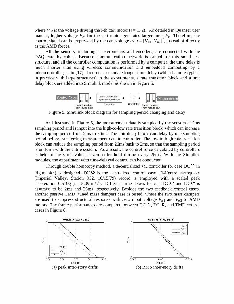
where Vmi is the voltage driving the i-th cart motor (i = 1, 2). As detailed in Quanser user

manual, higher voltage Vmi for the cart motor generates larger force Fci. Therefore, the

control signal can be expressed by the cart voltage as u = [Vm1, Vm2]T, instead of directly

as the AMD forces.

All the sensors, including accelerometers and encoders, are connected with the

DAQ card by cables. Because communication network is cabled for this small test

structure, and all the controller computation is performed by a computer, the time delay is

much shorter than using wireless communication and embedded computing by a

microcontroller, as in [17]. In order to emulate longer time delay (which is more typical

in practice with large structures) in the experiments, a rate transition block and a unit

delay block are added into Simulink model as shown in Figure 5.

Figure 5. Simulink block diagram for sampling period changing and delay

As illustrated in Figure 5, the measurement data is sampled by the sensors at 2ms

sampling period and is input into the high-to-low rate transition block, which can increase

the sampling period from 2ms to 26ms. The unit delay block can delay by one sampling

period before transferring measurement data to controller. The low-to-high rate transition

block can reduce the sampling period from 26ms back to 2ms, so that the sampling period

is uniform with the entire system. As a result, the control force calculated by controllers

is held at the same value as zero-order hold during every 26ms. With the Simulink

modules, the experiment with time-delayed control can be conducted.

Through double homotopy method, a decentralized ∞ controller for case DC in

Figure 4(c) is designed. DC is the centralized control case. El-Centro earthquake

(Imperial Valley, Station 952, 10/15/79) record is employed with a scaled peak

acceleration 0.519g (i.e. 5.09 m/s2). Different time delays for case DC and DC is

assumed to be 2ms and 26ms, respectively. Besides the two feedback control cases,

another passive TMD (tuned mass damper) case is tested, where the two mass dampers

are used to suppress structural response with zero input voltage Vm1 and Vm2 to AMD

motors. The frame performances are compared between DC , DC , and TMD control

cases in Figure 6.

(a) peak inter-story drifts

(b) RMS inter-story drifts

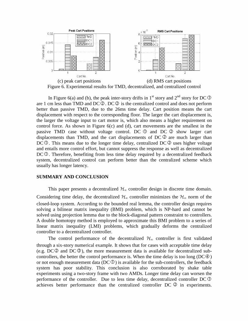
(c) peak cart positions

(d) RMS cart positions

Figure 6. Experimental results for TMD, decentralized, and centralized control

In Figure 6(a) and (b), the peak inter-story drifts in 1st story and 2

nd story for DC

are 1 cm less than TMD and DC . DC is the centralized control and does not perform

better than passive TMD, due to the 26ms time delay. Cart position means the cart

displacement with respect to the corresponding floor. The larger the cart displacement is,

the larger the voltage input to cart motor is, which also means a higher requirement on

control force. As shown in Figure 6(c) and (d), cart movements are the smallest in the

passive TMD case without voltage control. DC and DC show larger cart

displacements than TMD, and the cart displacements of DC are much larger than

DC . This means due to the longer time delay, centralized DC uses higher voltage

and entails more control effort, but cannot suppress the response as well as decentralized

DC . Therefore, benefiting from less time delay required by a decentralized feedback

system, decentralized control can perform better than the centralized scheme which

usually has longer latency.

SUMMARY AND CONCLUSION

This paper presents a decentralized ∞ controller design in discrete time domain.

Considering time delay, the decentralized ∞ controller minimizes the ∞ norm of the

closed-loop system. According to the bounded real lemma, the controller design requires

solving a bilinear matrix inequality (BMI) problem, which is NP-hard and cannot be

solved using projection lemma due to the block-diagonal pattern constraint to controllers.

A double homotopy method is employed to approximate this BMI problem to a series of

linear matrix inequality (LMI) problems, which gradually deforms the centralized

controller to a decentralized controller.

The control performance of the decentralized ∞ controller is first validated

through a six-story numerical example. It shows that for cases with acceptable time delay

(e.g. DC and DC ), the more measurement data is available for decentralized sub-

controllers, the better the control performance is. When the time delay is too long (DC )

or not enough measurement data (DC ) is available for the sub-controllers, the feedback

system has poor stability. This conclusion is also corroborated by shake table

experiments using a two-story frame with two AMDs. Longer time delay can worsen the

performance of the controller. Due to less time delay, decentralized controller DC

achieves better performance than the centralized controller DC in experiments.

Because the proposed double homotopy method is heuristic, significant amount of future

studies are needed to compare its performance with other existing methods for

decentralized control design.

ACKNOWLEDGEMENT

The authors are grateful for the support National Natural Science Foundation of

China (grant number 51121005 and 50708016) and National Earthquake Special

Founding of China (grant number 200808074), and also appreciate the experiment device

supported by Structural Health Monitoring and Control Lab in Faculty of Infrastructure

Engineering, Dalian University of Technology. Dr. Yang Wang is supported by the U.S.

National Science Foundation CAREER Award CMMI-1150700. Any opinions, findings,

and conclusions or recommendations expressed in this publication are those of the

authors and do not necessarily reflect the view of the sponsors. In addition, The authors

would like to thank Prof. Chin-Hsiung Loh and Dr. Kung-Chun Lu of the National

Taiwan University, as well as Dr. Pei-Yang Lin of NCREE, for generously providing the

numerical model of the six-story example structure.

REFERENCES

1. Adeli H. Wavelet-Hybrid Feedback-Least Mean Square Algorithm for Robust Control of

Structures. Journal of Structural Engineering 2004; 130(1):128-137.

2. Kim Y., Hurlebaus S.,Langari R. Model-Based Multi-input, Multi-output Supervisory Semi-

active Nonlinear Fuzzy Controller. Computer-Aided Civil and Infrastructure Engineering

2010; 25(5):387-393.

3. Lin C. C., Chen C. L.,Wang J. F. Vibration Control of Structures with Initially Accelerated

Passive Tuned Mass Dampers under Near-Fault Earthquake Excitation. Computer-Aided Civil

and Infrastructure Engineering 2010; 25(1):69-75.

4. Spencer B. F., Jr.,Nagarajaiah S. State of the Art of Structural Control. Journal of Structural

Engineering 2003; 129(7):845-856.

5. Sandell N., Jr., Varaiya P., Athans M.,Safonov M. Survey of decentralized control methods for

large scale systems. Automatic Control, IEEE Transactions on 1978; 23(2):108-128.

6. Siljak D. D. Decentralized Control of Complex Systems. Academic Press: Boston, 1991.

7. Siljak D. D. Decentralizedcontrol and computations: status and prospects. Annual Reviews in

Control 1996; 20:131-141.

8. Lynch J. P.,Law K. H. Decentralized control techniques for large scale civil structural systems.

Proceedings of the 20th International Modal Analysis Conference, Los Angeles, CA, 2002.

9. Xu B., Wu Z. S.,Yokoyama K. Neural networks for decentralized control of cable-stayed

bridge. Journal of Bridge Engineering 2003; 8(4):229-236.

10. Swartz R. A.,Lynch J. P. Redundant Kalman Estimation for a Distributed Wireless Structural

Control System. Proceedings of the US-Korea Workshop on Smart Structures Technology for

Steel Structures, Seoul, Korea, 2006.

11. Rofooei F. R.,Monajemi-Nezhad S. Decentralized control of tall buildings. The Structural

Design of Tall and Special Buildings 2006; 15(2):153-170.

12. Lu K. C., Loh C. H., Yang J. N.,Lin P. Y. Decentralized sliding mode control of a building

using MR dampers. Smart Materials and Structures 2008; 17(5):055006.

13. Ma T. W., Xu N. S.,Tang Y. Decentralized robust control of building structures under seismic

excitations. Earthquake Engineering & Structural Dynamics 2008; 37(1):121-140.

14. Loh C. H.,Chang C. M. Application of centralized and decentralized control to building

structure: analytical study. Journal of Engineering Mechanics 2008; 134(11):970-982.

15. Wang Y., Law K. H.,Lall S. Time-delayed decentralized H∞ controller design for civil

structures: a homotopy method through linear matrix inequalities. Proceedings of the 2009

American Control Conference (ACC 2009), St. Louis, MO, USA, 2009.

16. Wang Y. Time-delayed dynamic output feedback H∞ controller design for civil structures: a

decentralized approach through homotopic transformation. Structural Control and Health

Monitoring 2011; 18(2):121-139.

17. Wang Y., Swartz R. A., Lynch J. P., Law K. H., Lu K.-C.,Loh C.-H. Decentralized civil

structural control using real-time wireless sensing and embedded computing. Smart Structures

and Systems 2007; 3(3):321-340.

18. Gahinet P.,Apkarian P. A linear matrix inequality approach to H∞ control. International

Journal of Robust and Nonlinear Control 1994; 4(4):421-448.

19. VanAntwerp J. G.,Braatz R. D. A tutorial on linear and bilinear matrix inequalities. Journal of

Process Control 2000; 10(4):363-385.

20. Kocvara M.,Stingl M. PENNON - A Code for Convex Nonlinear and Semidenite

Programming. Optimization Methods and Software 2003; 18(3):317-333.

21. Mehendale C. S.,Grigoriadis K. M. A double homotopy method for decentralised control

design. International Journal of Control 2008; 81(10):1600 - 1608.