Embed Size (px)
Citation preview
NONABELIANIZATION, SPECTRAL DATA AND CAMERAL DATA
Benedict John Roland Morrissey
A DISSERTATION
in
Mathematics
Presented to the Faculties of the University of Pennsylvania in Partial Fulfillmentof the Requirements for the Degree of Doctor of Philosophy
2020
Supervisor of Dissertation
Ron DonagiProfessor of Mathematics
Co-Supervisor of Dissertation
Tony PantevClass of 1939 Professor of Mathematics
Graduate Group Chairperson
Julia Hartmann, Professor of Mathematics
Dissertation Committee:Ron Donagi, Professor of MathematicsTony Pantev, Class of 1939 Professor of MathematicsJustin Hilburn, Postdoctoral Fellow, University of Waterloo and Perimeter Institutefor Theoretical Physics
Acknowledgments
I would like to thank Ron Donagi for support, many discussions of mathematics, and in
particular for making sure I had thought through examples during my time at UPenn.
I would also like to thank Tony Pantev for support, and discussions of mathematics,
particularly as related to recent work on Stokes structures.
From prior to my PhD I would like to thank Masoud Kamgarpour, Peter Bouwknegt,
Jarod Alper, Tim Trudgian, and the NZMOC, for help and support in my matheamtics
career prior to me coming to UPenn.
I would like to thank the many people I have had discussions with on both the math-
ematics in this thesis, and the mathematics that has not made it into this thesis. A sadly
incomplete list of people who are not mentioned elsewhere would include M. Abouzaid,
J. Block, A. Fenyes, D. Gaiotto, B. Gammage, J. Lurie, T. Mochizuki, A. Neitzke, and
Ngo B.-C.
I would like to thank Mauro Porta and Justin Hilburn for running the derived geometry
and geometric representation learning seminars, and many discussions since then.
I would like to thank my friends Hadleigh Frost, Trang Nguyen, Minh–Tam Trinh,
and Yifei Zhao, for long running mathematics discussions. I would like to thank my
ii

friends Sukjoo Lee and Matei Ionita for innumerable conversations on mathematics and
otherwise, and for being part of many learning seminars with me over the past five years.
I would also like to thank Matei for the long term collaboration [23] on which this thesis
is based, and feedback on a draft of this thesis. I would also like to thank everyone who
came to and talked at the various learning seminars I’ve been involved with at UPenn.
I would like to thank Simon and Nan for hosting me over several winter breaks. Finally
I would like to thank my mother Janet for her long term support.
iii
ABSTRACT
NONABELIANIZATION, SPECTRAL DATA AND CAMERAL DATA
Benedict John Roland Morrissey
Ron Donagi
Tony Pantev
This thesis surveys parts of the forthcoming joint work [23] in which the non-abelianization
map of [16] was extended from the case of G = SL(n) and G = GL(n) to the case of
arbitrary reductive algebraic groups. The non-abelianization map is an algebraic map
from a moduli space of certain N -local systems on the complement of a divisor P in a
punctured Riemann surface X, to the moduli space of G-local systems on X.
iv
Contents
1 Introduction 1
1.1 Outline . . . . . . . . . . . . . . . . . . . . . . . . . . . . . . . . . . . . . 6
2 Local Systems, Hitchin base, and Lie Algebras 8
2.1 Local Systems and Their Moduli . . . . . . . . . . . . . . . . . . . . . . . 8
2.2 The Hitchin Base . . . . . . . . . . . . . . . . . . . . . . . . . . . . . . . . 10
2.3 Algebraic Groups . . . . . . . . . . . . . . . . . . . . . . . . . . . . . . . . 12
3 Spectral and Cameral Networks 15
3.1 Abstract Cameral Networks . . . . . . . . . . . . . . . . . . . . . . . . . . 16
3.2 Spectral Networks . . . . . . . . . . . . . . . . . . . . . . . . . . . . . . . 18
3.3 WKB Cameral Networks . . . . . . . . . . . . . . . . . . . . . . . . . . . . 20
3.3.1 The Hitchin Base and Differentials . . . . . . . . . . . . . . . . . . 21
3.3.2 Behaviour of Differentials near D ⊂ Xc . . . . . . . . . . . . . . . 24
4 Nonabelianization 28
4.1 Moduli Spaces of N and T Local Systems . . . . . . . . . . . . . . . . . . 28
4.2 The S-monodromy Condition . . . . . . . . . . . . . . . . . . . . . . . . . 31
v
4.3 The Nonabelianization Map . . . . . . . . . . . . . . . . . . . . . . . . . . 34
4.3.1 Stokes Factors for Initial Stokes Lines . . . . . . . . . . . . . . . . 37
4.3.2 Stokes Factors for New Stokes Lines . . . . . . . . . . . . . . . . . 39
4.3.3 Reglue Map . . . . . . . . . . . . . . . . . . . . . . . . . . . . . . . 42
5 Spectral Descriptions of Nonabelianization 44
5.1 Spectral and Cameral Covers . . . . . . . . . . . . . . . . . . . . . . . . . 44
5.1.1 Constructing Spectral Covers from Cameral Covers . . . . . . . . . 45
5.1.2 Local systems on Spectral covers from N -local systems . . . . . . . 46
5.2 Path Detour Rules and Miniscule Representations . . . . . . . . . . . . . 48
5.3 Spectral Description of N -Local Systems For Classical Groups . . . . . . 52
5.3.1 The Case of GL(n), and SL(n) . . . . . . . . . . . . . . . . . . . . 53
5.3.2 The Case of Sp(2n) . . . . . . . . . . . . . . . . . . . . . . . . . . 58
5.3.3 The case of SO(2n) . . . . . . . . . . . . . . . . . . . . . . . . . . 62
5.3.4 The case of SO(2n+ 1) . . . . . . . . . . . . . . . . . . . . . . . . 68
vi
Chapter 1
Introduction
Non-abelianization refers to the “co-ordinate charts” in the form of maps from the moduli
of certain Gm-local systems on a curve X\R (for a divisor R ⊂ X) to the moduli of GL(n)
or SL(n) local systems on X, where X → X is an n : 1 cover, and X is a punctured
Riemann surface. These are referred to as coordinate charts because complex analytically
one can describe the moduli space of Gm-local systems via it’s monodromy as (Gm)a/Gm
for some number a, with the action of Gm being trivial1. These co-ordinate charts are
conjectured to be hyperkahler [16, 13, 17] when restricted to holomorphic symplectic
leaves of the Poisson moduli spaces of local systems, and allow one to describe wall
crossing phenomena in the BPS spectrum of a 4d N = 2 field theories of class S with
gauge group SL(n). These wall crossing phenomena were related to coordinate charts
in the series of papers [18, 17, 16, 14, 13, 15]. This thesis surveys the extension of the
non-abelianization construction to the setting of reductive algebraic groups, as developed
in the joint work [23].
1We consider the stacky quotient, so this is not simply equivalent to (Gm)a
1
In the case where we consider non-abelianization for the group SL(2), subject to a
modification that involves working on the unit tangent bundle of a punctured Riemann
surface, these coordinates correspond [11, 21, 17] to the Fock–Goncharov coordinates [12]
on the complexification of Teichmuller space. An extension of these methods to compact
surfaces for G = SL(2),R) in [11] recovers Thurston’s shear-bend coordinates [35].
The covers X → X are spectral covers in the sense of [20], and are constructed from
points in the Hitchin base for the group GL(n) or SL(n). Fibers of the Hitchin moduli
space are described in terms of Gm-bundles (line bundles) on the spectral curve in this
setting. This was generalized in the series of works [8, 32, 10, 9]. The paper [9] describes
fibers of the Hitchin system in terms of N -shifted, weakly W -equivariant T -bundles on a
curve called the cameral cover X → X in the case where X is smooth. The curve X is
constructed from a point in the Hitchin base.
Analogously to the case of the description of Hitchin fibers, we can extend the non-
abelianization map of [16] to the setting of arbitrary reductive algebraic groups G by
replacing the moduli space of certain Gm-local systems on2 X\Rρ to the moduli space
of N -shifted weakly W -equivariant T -local systems on X\R (for R ⊂ X the ramification
divisor of X → X). We have to reduce to a subset of such T -local systems that satisfy a
condition which we call the S-monodromy condition introduced in 4.2.
We will now describe briefly how the non-abelianization construction works. The
rough idea of non-abelianization is that we modify a local system on what is topologically
a two dimensional surface by “cutting and regluing” along a series of one dimensional loci,
that together form a piece of data called a spectral network. The following is a simplified
2Rρ is here the ramificarion divisor of X → X
2
example
Example 1.0.1 (Non-abelianization by “cutting and regluing” on S1.). Suppose we have a
G-local system E → S1. Let [0, 1]p−→ S1 be the surjective map such that p(0) = p(1), and
the preimage of every point other than p(1) consists of a single element. Informally words
p identifies [0, 1] with the circle S1 being “cut” at the point p(0). We can then consider
p∗E as being the G-local system E “cut” at p(0).
If we have an isomorphism ofG-torsors a : p∗E|0∼=−→ p∗E|1, then p∗E/{p∗E|0 a−→ p∗E|1} is
a G-local system on S1. Informally we refer to this procedure of gaining a new local system
on S1 as regluing. Note that if the automorphism we reglue by is the monodromy around
the circle, and the direction we glue by is the opposite to the direction with respect to
which we described the monodromy, we will get a G-local system with trivial monodromy,
which can hence be extended to a G-local system on the disc D with boundary ∂D = S1.
In the construction of non-abelianization, the types of G-local system we consider will
be those that have been induced from N -local systems.
When we do this construction on the topological space underlying a punctured Rie-
mann surface X the locus on which we “cut and reglue” can be more complicated. The
locus we use is a spectral network, which [16] described how to construct from certain
points in the Hitchin base for G = GL(n) or G = SL(n), and [27] described how to con-
struct in the case of groups of type ADE, with the exception of E8. The cases of GL(n)
and SL(n) spectral networks had already appeared in the setting of exact WKB analysis
under the name of Stokes graphs, see e.g. [25, 24, 5, 34, 1, 2, 22, 3]. Unfortunately it
is not entirely clear for G �= SL2, PGL2, GL(2) for which points in the Hitchin base
the construction of a spectral network works. We do not resolve this point. We define
3
spectral networks for arbitrary reductive algebraic groups G, starting from appropriate
points in the Hitchin base in chapter 3 following [23].
Our main result follows:
Construction–Theorem 1.0.2 (See Construction–Theorem 5.15 of [23], and Construc-
tions 4.3.9, Equation 4.3.1 and Theorem 4.3.10 of this document.). To an abstract spectral
network (see definition 3.2.1) on a punctured Riemann surface X with cameral cover X,
the maps sWKB defined in equation 4.3.1, and the reglue map of Construction 4.3.9 pro-
vide a map
LocX\R,SN (X\P ) → LocG(X),
where LocX,SN (X\P ) refers to the moduli of N -local systems on X\P corresponding to
the W -bundle X\R → X\P , satisfying a restriction on the monodromy called the S-
monodromy condition defined in 4.2.2. Note that P and R are the branch and ramification
divisors of the map X → X, where X is smooth.
The moduli of N -local systems used in Theorem 1.0.2 can instead be described in
terms of T -local systems on the cameral cover X\R, as the following theorem shows. We
reference chapter 4 for precise definitions of the moduli spaces involved.
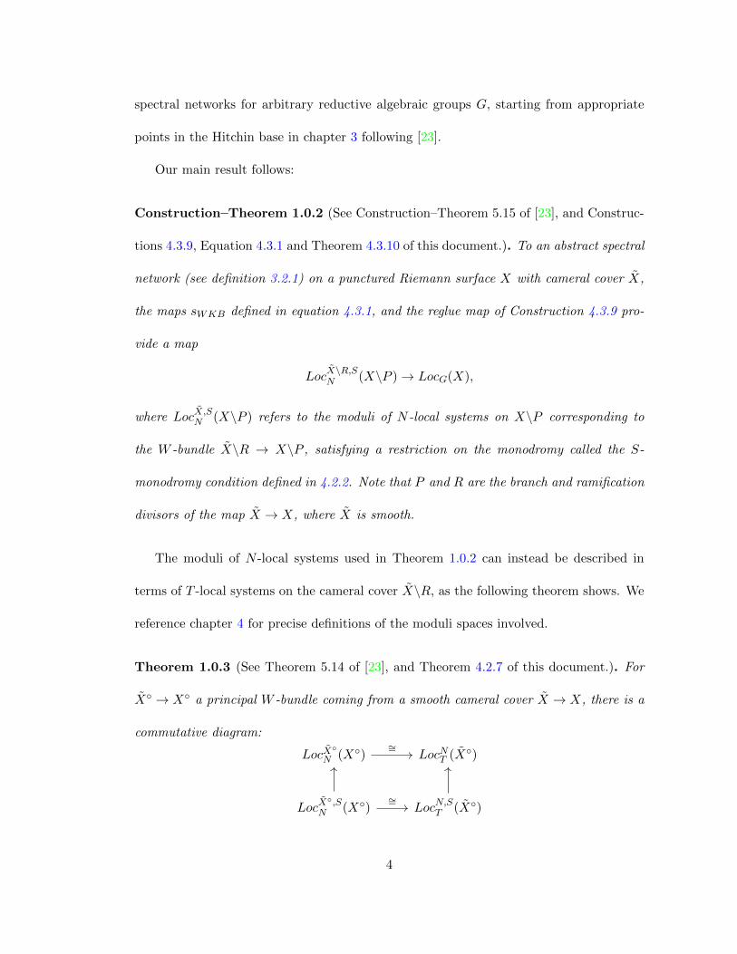
Theorem 1.0.3 (See Theorem 5.14 of [23], and Theorem 4.2.7 of this document.). For
X◦ → X◦ a principal W -bundle coming from a smooth cameral cover X → X, there is a
commutative diagram:
LocX◦
N (X◦) LocNT (X◦)
LocX◦,S
N (X◦) LocN,ST (X◦)
∼=
∼=
4
Here LocX◦
N (X◦) is the moduli space of N -local systems on X◦ which correspond to the W -
bundle X◦, LocX◦,S
N (X◦) is the moduli space of such N -local systems which also satisfy the
S-monodromy condition. The space LocNT (X◦) is the moduli space of N -shifted, weakly
W -equivariant T -local systems on X◦, and LocN,ST (X◦) is the moduli space of T -local
systems which also satisfy the S-monodromy condition.
Finally in chapter 5 we consider how to describe these moduli spaces in spectral terms.
One of the results is the compatibility between the non-abelianization construction
of Construction–Theorem 1.0.2, and the path detour non-abelianization construction of
[16, 27], described here in construction 5.2.2, given by the following commutative diagram.
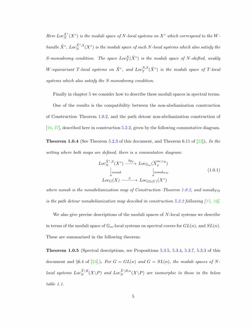
Theorem 1.0.4 (See Theorem 5.2.3 of this document, and Theorem 6.11 of [23]). In the
setting where both maps are defined, there is a commutative diagram:
LocX◦,S
N (X◦) LocGm(Xne,◦Rρ )
LocG(X) LocGL(V )(X◦)
Spρ
nonab nonabPD
ρ
(1.0.1)
where nonab is the nonabelianization map of Construction–Theorem 1.0.2, and nonabPD
is the path detour nonabelianization map descibed in construction 5.2.2 following [27, 16].
We also give precise descriptions of the moduli spaces of N -local systems we describe
in terms of the moduli space of Gm-local systems on spectral covers for GL(n), and SL(n).
These are summarized in the following theorem:
Theorem 1.0.5 (Spectral descriptions, see Propositions 5.3.5, 5.3.4, 5.3.7, 5.3.3 of this
document and §6.4 of [23].). For G = GL(n) and G = SL(n), the moduli spaces of N -
local systems LocX\RN (X\P ) and Loc
X\R,αN (X\P ) are isomorphic to those in the below
table 1.1.
5
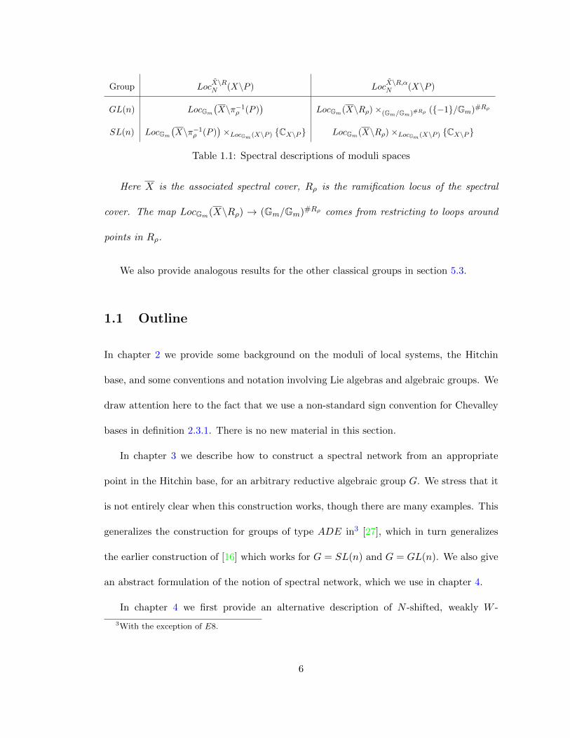
Group LocX\RN (X\P ) Loc
X\R,αN (X\P )
GL(n) LocGm
�X\π−1
ρ (P )�
LocGm(X\Rρ)×(Gm/Gm)#Rρ ({−1}/Gm)#Rρ
SL(n) LocGm
�X\π−1
ρ (P )�×LocGm (X\P ) {CX\P } LocGm(X\Rρ)×LocGm (X\P ) {CX\P }
Table 1.1: Spectral descriptions of moduli spaces
Here X is the associated spectral cover, Rρ is the ramification locus of the spectral
cover. The map LocGm(X\Rρ) → (Gm/Gm)#Rρ comes from restricting to loops around
points in Rρ.
We also provide analogous results for the other classical groups in section 5.3.
1.1 Outline
In chapter 2 we provide some background on the moduli of local systems, the Hitchin
base, and some conventions and notation involving Lie algebras and algebraic groups. We
draw attention here to the fact that we use a non-standard sign convention for Chevalley
bases in definition 2.3.1. There is no new material in this section.
In chapter 3 we describe how to construct a spectral network from an appropriate
point in the Hitchin base, for an arbitrary reductive algebraic group G. We stress that it
is not entirely clear when this construction works, though there are many examples. This
generalizes the construction for groups of type ADE in3 [27], which in turn generalizes
the earlier construction of [16] which works for G = SL(n) and G = GL(n). We also give
an abstract formulation of the notion of spectral network, which we use in chapter 4.
In chapter 4 we first provide an alternative description of N -shifted, weakly W -
3With the exception of E8.
6
equivariant T -local systems on X\R in terms of N -local systems on X\P (where P is
the branch locus), which correspond to the given cameral cover X\R. We also describe a
condition that we call the S-monodromy condition, that we also have to apply. We then
describe the construction of the non-abelianization map using the data of an (abstract)
spectral network.
In chapter 5 we describe the moduli spaces of N -shifted, weakly W -equivariant T -local
systems on X\R satisfying the S-monodromy condition in terms of Gm-local systems
on spectral covers for the classical groups. We also describe the relation between the
non-abelianization map we construct here and the path detour rule construction of non-
abelianization given in [16] for SL(n) and GL(n), and proposed for simply laced groups
in [27], in section 5.2. .
7
Chapter 2
Local Systems, Hitchin base, and
Lie Algebras
The purpose of this chapter is to recall some well known theory about local systems and
their moduli, the Hitchin base, and Lie algebras that will be used in the sequel.
2.1 Local Systems and Their Moduli
Let X = Xc\D be a punctured Riemann surface, where Xc is a compact Riemann surface,
and D ⊂ Xc is a non-zero reduced divisor.
Definition 2.1.1. A G-local system on X is a locally constant sheaf E of sets with right
G-action on X, such that for all x ∈ X, Ex is a G-torsor.
Associated to such a local system, a choice of x ∈ X, and a choice of trivialization
x� ∈ Ex, we can construct a representation ρ : π1(X,x) → G, defined by ρ(γ) = g, where
g ∈ G is the unique element such that x�g is the parallel transport of x� along γ.
8
Changing the choice of x ∈ X, and changing the choice of trivialization of Ex has the
affect of conjugating the representation ρ constructed above.
Conversely given a representation ρ : π1(X) → G, we can construct a G-local system
on X, by taking the quotient Xun ×G/π1(X), where Xun → X is the universal cover of
X, and π1(X) acts diagonally by deck transformations and by the representation ρ.
Definition 2.1.2 (Classical Moduli stack of Local systems). We define the lassical1 mod-
uli space of G-local systems as
LocG(X)cl := HomGrp(π1(X), G)/G,
where we are taking the stacky quotient.
Remark 2.1.3. We note thatHomGrp(π1(X), G) is an affine scheme. This is because we re-
call that there is a choice of generators (called the canonical cycles) α1,β1, ...,αg,βg, γ1, ..., γd
(g is the genus of X, and d = deg(D)) of π1(X), such that we have an isomorphism:
π1(X) =
�α1,β1, ...,αg,βg, γ1, ..., γd
�����
g�
i=1
[αi,βi]
d�
i=1
γi = Id
�. (2.1.1)
We hence can write
HomGrp(π1(X), G) �→ G2g+d � (xα1 , xβ1 , ..., xαg , xβg , xγ1 , ..., xγd)
as being cut out by the equation�g
i=1[xαi , xβi]�d
j=1 xγj = Id.
We want to consider the (derived) moduli space of G-local systems on X. Note that
the role of derived geometry in this thesis is very small, and can be ignored if desired,
see remark 2.10 of [23] for a precise statement about when use of derived geometry is
necessary.
1We use classical here in the sense that we are not referring to the derived moduli space.
9
Definition 2.1.4 (Betti Stack). The derived stack XB is the constant functor dSchop →
Top, from the opposite category2 of derived schemes to the category of topological spaces,
such that it maps all derived schemes to the topological space underlying the punctured
Riemann surface X.
For � a topological space we denote �B the constant functor dSchop → Top, which
maps all derived schemes to the topological space �.
Definition 2.1.5 (Moduli of G-local systems). We define the moduli space of G-local
systems as the (derived) mapping stack
LocG(X) := HomdSt(X,BG).
See e.g. §19.1 of [28] for an overview of derived mapping stacks.
In [36] it is shown that t0(LocG(X)) = LocG(X)cl, where t0 is the truncation functor
from derived stacks to stacks in the ordinary sense.
2.2 The Hitchin Base
The Hitchin base associated to Xc and the line bundle KXc(D), for D a non-zero reduced
divisor is the space A := Γ(Xc, tKXc (D)/W ), where tKXc (D) := Tot(KXc(D))×Gm t.
Definition 2.2.1. Given a point a ∈ A we define the associated cameral cover Xc → Xc
as the pullback:
Xca tL
Xc tL/W
a
π
a
(2.2.1)
2Here category should be understood to mean (∞, 1)-category in the sense of [29].
10
We will often simply denote a cameral cover as Xc if we do not want to emphasize
the point of the Hitchin base it is associated to. We also denote X := Xc ×Xc X. We
also refer to X as a cameral cover. In the case where X is reduced, we let R ⊂ X and
P ⊂ X be the ramification and branch divisors of X. We let X◦ := ReBlR(X), and
X◦ := ReBlP (X) be the real blow ups at these divisors3. We will also refer to X◦ → X◦
as a cameral cover.
The cameral cover X has an action of W induced by the action of W on t. If X is
reduced, and the map X → X is unramified, then X → X is a principal W -bundle. In
particular X◦ → X◦ is a principal W -bundle.
Definition 2.2.2. We define the Zariski openA♦ ⊂ A as the subset ofA = Γ(Xc, tKXc (D)/W ),
where X intersects�∪α∈Φ (Hα)KXc (D)
�/W ⊂ tKXc (D)/W transversely.
Here (Hα)KXc (D) denotes Tot(KXc(D))×Gm Hα.
Lemma 2.2.3 (See [10, 30]). For a ∈ A♦, the cameral cover Xa is smooth. Furthermore
around the ramification points the map is locally modelled on A1z → A1
w, w �→ z2.
Proof. The transversality condition implies that X does not intersect the singular part
of�∪α∈Φ (Hα)KXc (D)
�, that is to say it does not intersect (Hα)KXc (D) ∩ (Hβ)KXc (D) for
any pair of roots α �= β. Then as each intersection with some (Hα)KXc (D) is transveral,
it is smooth, and the quotient by sα ∈ W is locally modelled on A1z/{±1} = A1
w, where
w = z2.
Lemma 2.2.4. The set A♦ ⊂ A is non-empty for the genus of Xc satisfying g ≥ 1 (recall
3To take the real blow up we consider the complex analytic manifold associated to the Riemann surface,
and consider the underlying real analytic space.
11
we assumed deg(D) ≥ 1). For X = P1 nonemptyness of A♦ holds if deg(D) ≥ 2.
Proof. We modify the proof of Proposition 4.6.1 of [30]. To adapt this proof to our
situation we need only show that KXc(D) is ample. This is the case under the conditions
imposed the lemma.
2.3 Algebraic Groups
Let G be a reductive algebraic group with maximal torus T ⊂ G. We denote by Φ the
root system, and N = NG(T ) the normalizer of T , and W = NG(T )/T the Weyl group.
We denote by
q : N → W (2.3.1)
the quotient map.
We now wish to introduce a version of Chevalley basis with a non-standard choice of
signs, which is more convenient for our purposes.
Definition 2.3.1 (Chevalley basis). Let g be a semisimple Lie algebra with root space
decomposition g = t⊕α∈Φ gα. A Chevalley basis is a set of elements:
• {hα}α a simple root. forming a basis of t.
• An element eα ∈ gα for each α ∈ Φ.
Furthermore for γ =�
i aiαi, with αi a simple root, we define hγ :=�
i aihi.
These elements are required to satisfy:
12
[hα, eγ ] = 2(α, γ)
(α,α)eγ , (2.3.2)
[eα, e−α] = −hα, (2.3.3)
[eα, eγ ] =
0 if α+ γ not a root,
±(pα,γ + 1)eα+γ if α+ γ is a root.
(2.3.4)
The number pα,γ in equation 2.3.4, denotes the largest integer with the property that
α− pα,γγ is a root.
Choose a Chevalley basis (see [7]) of the semisimple part of g – the Lie algebra of G.
For each root α ∈ Φ, we denote by
Iα : SL2 → G (2.3.5)
be the map of group corresponding to the map of Lie algebras
iα : sl2 → g
specified by the Chevalley basis, with iα(sl2) = span(eα, hα, e−α).
We now introduce some subgroups and elements that will be used in the sequel.
Definition 2.3.2. For a root α ∈ Φ, we define the abelian subgroup: Tα := Iα(TSL2) ⊂ T .
We denote by tα it’s Lie algebra.
Definition 2.3.3. We define nα ∈ N , for a root α ∈ Φ, as
nα := Iα
0 1
−1 0
.
13
Definition 2.3.4. We define TKer(α) to be the subgroup of T corresponding to the sub
Lie algebra
tKer(α) �→ tαα−→ C
which is the kernel of α.
14
Chapter 3
Spectral and Cameral Networks
We fix a reductive algebraic group G with chosen maximal torus T ⊂ G. We also fix a
Riemann surface with punctures X = Xc\D (where D �= ∅ is a reduced divisor on the
compact Riemann surface Xc). Spectral networks are a topological object consisting of a
union of oriented lines1 � ⊂ X. These lines are labelled by additional data. The networks
and the data are most easily described using cameral networks, which are topological
objects on a cameral cover X → X, labelled by roots, which are compatible with the
action of W on X, and the root system. In this chapter we introduce this construction
following [23].
We also describe how these abstract topological objects can be constructed using
certain points of the Hitchin base associated to the group G, and the line bundle KXc(D).
In the case where G = SL(2) we essentially recover the trajectories of a quadratic
differential. For groups of type ADE, we recover the definitions of [27], and that of [16]
1By lines we mean one dimensional submanifolds. We are here considering the two dimensional real
analytic manifold underlying the complex analytic manifold/scheme X.
15
in the case of G = GL(n) or G = SL(n).
3.1 Abstract Cameral Networks
We firstly introduce the notion of 2d scattering diagrams which provide a local description
of cameral networks when multiple lines in the cameral network intersect.
We first introduce some additional terminology.
Definition 3.1.1. A set of roots C ⊂ Φ is convex if the cone Cone(C) := {a =
�αi∈C aiαi|ai ∈ R, ai ≥ 0}, does not contain any non-trivial vector subspace of t∨.
Definition 3.1.2. Let C ⊂ Φ be a set of roots, we define
ConvN(C) := {β ∈ Φ|β =�
i
aiαi, ai ∈ Z, ai ≥ 0}.
Definition 3.1.3. To each root α we let Uα denote the unipotent subgroup of G, with
Lie algebra being the weight space uα �→ g of the adjoint representation corresponding to
α.
Definition 3.1.4. A 2d scattering diagram is a set of oriented rays in the plane2, either
starting or ending at the origin, together with:
• A bijection between the set of incoming rays, and a convex set of roots C ⊂ Φ.
• A bijection between the set of outgoing rays and roots in ConvN(C).
Definition 3.1.5 (Abstract Cameral Networks, Essentially definition 4.4 of [23]). We
fix a smooth cameral cover X → X associated to a ∈ A♦, and denote its branch and
2Considered as an oriented manifold.
16
ramification divisors by P and R respectively. We denote by X◦ π−→ X◦ the principal W
bundle defined in definition 2.2.1, and also refer to this as the cameral cover.
An abstract cameral network W on X◦, is the data of
• A subspace X◦� �→ X◦, preserved under the action of W , such that the inclusion is
a homotopy equivalence.
• A union of a finite set of smooth oriented lines with single boundary {�i}i with
�i �→ X◦� �→ X◦, each labelled by a root αi ⊂ Φ. By a single boundary we
mean that the subset �i ⊂ X◦� can be described by i([0, 1)), for some smooth
i : [0, 1) → X◦� . These are required to have the following property: The closure
of � inside the closure�X◦�
�⊂ ReBlR∪π−1(D)(X
c) of X◦� in the real blow up of
Xc along both R and π−1(D), has to consist of � ∪ pt, where pt is a single point in
�X◦�
�\X◦� .
These are required to satisfy the following properties:
• Equivariance: Let � ⊂ W be a line in W labelled by α, then w(�) is in W, and has
the label w(α), for any w ∈ W .
• Behaviour at ramification points : For p ∈ P , and S1r ⊂ X◦ be a connected com-
ponent of the preimage of S1p , corresponding to a ramification point r ∈ X. There
are 6 lines of the cameral network that intersect S1r . The labels of these alternate
between α and −α, where these are the two roots such that at the ramification point
r, X intersects the root hyperplane (Hα)KXc(D). The orientation of these lines is
coming out of the circle S1r .
17
• Joints We call the intersection points of any pair of lines �i and �j , for i �= j, joints.
The set J of joints is finite. Furthermore at each joint the half of the tangent space
to incoming and outgoing lines that corresponds to the direction the line is either
coming in from or going out towards, together with the labels of their lines form a
2d scattering diagram in the sense of 3.1.4.
• Acyclicity Consider the directed graph, with vertices being the joints J the ramifi-
cation points R and the points d ∈ π−1(D), and edges being connected components
of W\J , with the orientation of the line providing the direction of the edge. We
require that this directed graph is acyclic.
• Non-denseness Let f : [0, 1] → X◦� intersect �i transversely at f(1/2) for all lines
�i � f(1/2). Then there is an open set 1/2 ∈ U ⊂ [0, 1], such that f(U)∩ W ⊂ 1/2.
We often abuse notation and write W to denote the topological space ∪i�i. We also
sometimes refer to the lines �i as Stokes lines. We hope this does not cause confusion.
Definition 3.1.6. For X◦� as above we can define X◦� := X◦�/W , this gives us a principal
W -bundle X◦� → X◦� . Furthermore it is clear that the inclusion X◦� �→ X◦ is a homotopy
equivalece.
3.2 Spectral Networks
Definition 3.2.1 (Abstract Spectral Network). An abstract spectral network W is the
set π∗W ⊂ X◦� , for W ⊂ X◦� �→ X◦ an abstract cameral network.
Note that we can still write W = ∪i�i for some lines �i �→ X◦� . These lines inherit
orientations from their preimages on X.
18
We can view these line segments �i as being labelled by a W -equivariant section of
Hom(X◦� |�i ,Φ).
We denote J = π∗J and call it the set of joints of the spectral network.
Remark 3.2.2. Picking a trivialization of the cameral cover away from a series of branch
cuts, gives labels of the lines by roots by precomposing the homomorphismHom(X◦� |�i ,Φ)
with the section trivializing the cameral cover. This recovers the labelling of lines of the
spectral network by roots, given such a choice of trivializations found in earlier work, in
particular in [27, 16].
Lemma 3.2.3 (Acyclicity). The directed graph with vertices being points of J ∪ P ∪D
and, and edges being connected components of W, with orientations inherited from the
orientations of lines of the spectral network. Then this graph is acyclic.
Proof. Suppose otherwise. Then we can lift a cycle in this graph, which includes a point
x ∈ (J ∪ P ∪D) ⊂ X to a cycle in the analogous graph (which we will call the cameral
graph) defined using the cameral network. This gives a path in the cameral graph between
the vertices correpsonding to two preimages x1 and x2 of x. We can commpose this
with the lift of the cycle starting at x2. Iterating this process as there are finitely many
preimages of x we will obtain a cycle contradicting the acyclicity requirement of definition
3.1.5.
Lemma 3.2.4. Consider the directed graph, with vertices being the union of joints J and
branch points P , and edges being connected components of W\J , with the orientation of
the line providing the direction of the edge.
19
There is a filtration F•(J ∪P ) on J ∪P (the vertices of this graph), with the property
that F0(J ∪ P ) = P , and the property that any edge ending at a vertex in Fm(J ∪ P )
starts at a vertex in Fm−1(J ∪ P ).
Proof. Lemma 3.2.3 shows that the graph with vertices being the joints and the circles S1p
(p ∈ P ) and edges being the connected components of W\J is an acyclic directed graph.
The local behaviour of the cameral network around ramification points shows that
there are no incoming edges to the vertices associated to the branch points p ∈ P .
It is well known that in this situation there is a filtration on the edges of the graph
which has the desired properties, in particular a proof can be found in lemma 4.5 of
[23].
Definition 3.2.5. We use the filtration F•J on joints to define a filtration F•W on
connected components of W\J as follows:
We define FiW to consist of all connected components of W\J that start (using the
orientation of the line) at a joint in FiJ .
Note that as there are finitely many joints, and finitely many lines, this filtration is
eventually constant, that is there is N >> 0, such that ∀m ≥ N , we have FmW = FNW.
3.3 WKB Cameral Networks
In this section an iterative procedure to define lines �i ⊂ X◦, starting from a point in the
Hitchin base. In good situations, after restricting to X◦� �→ X◦, this will give an abstract
cameral network in the sense of definition 3.1.5.
20
3.3.1 The Hitchin Base and Differentials
Construction 3.3.1. Let α ∈ Φ be a root, we construct a differential form χα on Xa.
Consider the map:
Xca
a−→ tKXc(D)
α−→ Tot(KcX(D))
This provides a map Xca → π∗KXc(D) → KXc(π∗(D)). We denote this differential, and its
restriction to X, by χa.
Associated to the differential χa is a real projective vector field Vα ∈ Γ(X, T X/R+),
defined as follows:
v ∈ [Vα] ⊂ TX (3.3.1)
if χα(v) ∈ R+.
We now provide what we will call the WKB construction of an abstract cameral
network, starting at certain points a ∈ A♦. We stress that this will not work starting at
an arbitrary point, and for G �= SL(2), PGL(2) the precise nature of the locus of points
where this construction does not work is unclear. However there is a wealth of examples
in e.g. [16, 27] of cases where this construction works for simply laced groups. More
examples can be produced by the software [26] which draws spectral networks for simply
laced groups.
We break this construction into two parts (constructions 3.3.2 and 3.3.7). The first
consists of drawing lines on X◦, and the second consists of restricting to a specified subset
X◦� ⊂ X◦.
Construction 3.3.2 (Part 1 of the WKB Construction). We start with a point a ∈ A♦,
and construct the associated smooth cameral cover X. We then construct the modified
21
version X◦ → X◦, which is a principal W -bundle.
This part is a two step construction, firstly we draw what we call the“initial” Stokes
lines, which start at the preimages of S1p , for p ∈ P . We then iteratively draw what we
call “new” Stokes lines which start where Stokes lines intersect.
This part of the construction does not work for arbitrary a ∈ A♦, and we end with a
list of points that can stop the iteration, or in which the produced result is unsuccessful.
• Firstly we take the closure in X◦, of for each r ∈ R ⊂ X the trajectories of the
projective vector field χα (as oriented, unparameterized lines), where α is a root
such that a(r) ∈ (Hα)KXc(D). We label such a line by the root α.
• We then iterate the following step, assuming that none of the phenomena in the list
below occur. For each intersection J (which we again call a joint), where one of the
lines produced in the previous step intersects another line, we draw new trajectories
of the projective vector field Vα starting at J for each α ∈ ConvNC , where C is the
set of lines passing through the joint J , assuming that these trajectories have not
already been drawn.
The behaviours that can cause the procedure to fail at one of the iterative steps follow:
• A loop forms, that is there is a non-contractible map of oriented manifolds S1 → ∪i�i
to the union of all lines so far produced.
• One of the lines drawn intersects one of the preimages of S1p , p ∈ P , or equivalently
if considering the line on X, contains a ramification point.
22
• A line drawn violates the non-denseness requirement of definition 3.1.5, with X◦�
replaced by X◦.
• At an intersection point the labels of the incoming roots do not form a convex set
in the sense of 3.1.1, or the tangent spaces of multiple incoming or outgoing lines
are equal so that the joints condition of definition 3.1.5 is violated.
We take the union of all labelled oriented lines produced in (possibly countably in-
finitely many) steps of the iterative process above.
Furthermore the construction can fail if after taking the union of the lines produced
at all steps of the iteration one of the following phenomena happens:
• The set of joints J has a limit point in X◦ (we allow it to have a limit point in Xc).
Lemma 3.3.3. The set of labelled, oriented curves produced in Construction 3.3.2 (if the
construction does not fail) is W -equivariant in the sense of the equivariance condition of
definition 3.1.5.
Proof. Immediate from the W -equivariance of the map Xc → tKXc (D), which means that
w∗χα = χwα, and hence w∗Vα = Vwα.
Lemma 3.3.4. The set of labelled, oriented curves produced in Construction 3.3.2 (as-
suming the construction does not fail) satisfies the “behaviour at ramification points”
condition of definition 3.1.5.
Proof. This is partly due to the requirement of terminating the construction if one of the
trajectories on X intersects a ramification point, and partly as a direct computation of
23
the local behaviour of the initial Stokes lines shows that this behaviour holds, as shown
in lemma 4.20 of [23].
We furthermore note that the acyclicity condition holds by assumption, if the con-
struction is successful. The finiteness condition on both joints, and on lines does not
necessarily hold, and if there are infinitely many lines the non-denseness condition does
not necessarily hold. Examples of cases where these do not hold are found in §5.5 of [16],
and are the reason for restricting to X◦� .
The idea of the second step of the WKB construction of an abstract cameral network
(construction 3.3.7 see also construction 3.3.2) is to pick a (W -equivariant) subspace
X◦� �→ X◦, such that the inclusion is a homotopy equivalence, and restrict the lines in
construction 3.3.2 to this subset. Before we do this, we prove some more results about
the behaviour of trajectories of Vα for some α near π−1(D) ⊂ Xc.
3.3.2 Behaviour of Differentials near D ⊂ Xc
Following the case of the Quadratic differential considered in, for example, [33, 6], we find
a condition (which we call condition R) under which we can appropriately restrict the
lines produced in construction 3.3.2 to a subspace X◦� �→ X◦.
Definition 3.3.5 (Condition R). We say that a ∈ A = Γ(Xc, tKXc (D)/W ) satisfies con-
dition R if for each d ∈ D using a local coordinate x, at d we can write
a(x) =
�W • (rd
dx
x)
�/W,
for rd ∈ t\�∪α∈Φα−1(iR)
�.
24
Note that as the subset�∪α∈Φα−1(iR)
�of t is W -equivariant, it does not matter which
lift rd of an element in t/W we use.
Proposition 3.3.6. Let a ∈ A♦ such that a satisfies condition R, and that construction
3.3.2 applied to a is successful. Then for any d ∈ D, there exists an open set d ∈ Bd ⊂ Xc
such that for any line � produced in construction 3.3.2 entering π−1(Bd) does not leave,
and furthermore any new Stokes line starting at a joint inside π−1(Bd) does not leave
π−1(Bd).
Proof. Note that by condition R, the covering Xc π−→ Xc is locally trivial around d ∈ D.
We will restrict to such a neighbourhood.
We will first outline how the trajectories of the Vα relate to quadratic differentials.
We note that for α ∈ Φ we factor π as
Xc → Xc/sαπα−→ Xc,
the differential form χα corresponds to a quadratic differential on Xc/sα:
Xc/sα → t/sα ⊗ π∗α(KXc(D)) → KXc/sα
(π−1α (D))/{±1}.
which corresponds to a section
qα ∈ Γ(Xc/sα, (KXc/sα(π−1(D)))⊗2)
To a quadratic differential q on a Riemann surface Y , we can associate a foliation of
Y by the curves γ : Rt → X such that:
d
ds
� s
t=t0
±√q(γ(t)) ∈ R. (3.3.2)
25
Note that this does not depend on parametrization, and furthermore the lines of this
foliation starting at ramification points correspond to lines of the SL(2) spectral network
associated to (Y, q).
The trajectories labelled by α on X are then, forgetting the orientation, given by the
pullback of sections of the folitation on X/sα determined by the quadratic differential qα.
Then by the analysis of the case of quadratic differentials found in [33] or section 3
of [6], for each α there is an open set Bd,α for which every line of the cameral network
labelled by α in π−1(Bd,α) either has tangent direction pointed towards a point in π−1(d)
or away from it3. Taking Bd := ∩αBd,αthe result follows up to the question of orientation
– we need to show that the tangent directions are always oriented towards d ∈ D. This
statement follows by induction on construction 3.3.2, and using lemma 4.14 of [23]. Firstly
note that any line entering the circle will has tangent direction towards d. Secondly lemma
4.14 of [23] says that any line starting at J ∈ Bd has tangent vector between the tangent
vectors of the incoming lines at J which by the induction hypothesis are oriented towards
d, and hence the tangent vector of the new Stokes line is oriented towards d.
See example 4.25 and proposition 4.32 in [23] for more details.
Construction 3.3.7 (Part II of the WKB construction). Starting at a point a ∈ A♦
satisfying condition R, firstly apply construction 3.3.2. Assuming this construction is
successful we then restrict to the lines intersecting X◦� := X◦\ ∪d∈D π−1(Bd), where Bd
is determined in proposition 3.3.6. We take the restrictions of the lines we keep to the
subset X◦� .3The uncertainty in the direction comes from the fact that the trajectories of a quadratic differential
are unoriented.
26
Theorem 3.3.8 (This is Proposition 4.19 in [23]). Apply constructions 3.3.2 and 3.3.7
to a point a ∈ A♦ satisfying condition R. Assume that this is successful, then we have
produced an abstract cameral network in the sense of definition 3.1.5.
Proof. Note that it is clear that X◦� �→ X◦ is preserved under the action of W , and is a
homotopy equivalence.
Furthermore by the assumption in construction 3.3.2 the joints J had no accumulation
point in X◦, hence there are only finitely many in X◦� . Hence there are only finitely many
lines.
We now need to prove the five conditions in definition 3.1.5. Note that the equivariance
and behaviour at ramification points conditions were proved in lemmas 3.3.3 and 3.3.4.
The joints condition follows by construction, and by the assumption about accumulation
points noted above. The acyclicity condition was required for success of construction
3.3.2. The non-denseness condition follows from the fact that there are finitely many
lines, and the non-denseness condition for the success of construction 3.3.2. The result
follows.
27
Chapter 4
Nonabelianization
4.1 Moduli Spaces of N and T Local Systems
Consider the short exact sequence
1 → T → N → W → 1
The morphism N → W induces a map LocN (X◦) → LocW (X◦), this allows us to
define the moduli of N -local systems that correspond to a given cameral cover as follows:
Definition 4.1.1 (Moduli N local systems corresponding to a cameral cover LocX◦
N (T )).
Let X◦ → X◦ be a principal W -bundle, we define
LocX◦
N (X◦) := LocN (X◦)×LocW (X◦) {X◦}.
Consider EN → X◦B×Y an N -bundle, equipped with an isomorphism EN/T ∼= X◦
B×Y .
This gives the map EN → EN/T × Y∼=−→ X◦ × Y the structure of a T -local system (using
the fact T is abelian). Letting Y = LocX◦
N (X◦), and EN be the universal object provides,
28
by the universal property, a map
LocX◦
N (X◦) → LocT (X◦). (4.1.1)
Clearly this is not an equivalence. We now follow [9] which considers the analogous
case in the setting of principal bundles rather than local systems to describe how to
upgrade the map in equation 4.1.1 to an isomorphism.
Firstly we make the following definition to be used in the sequel:
Definition 4.1.2. Let ET be a T -local system on X◦, we define the local system
AutX◦(ET ) := {(w, ρ)|w ∈ W, ρ : ET∼=−→ w∗ET },
where we are considering the action of w on X◦ given by the fact that X◦ → X◦ is a
principal W -bundle.
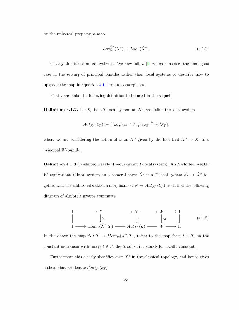
Definition 4.1.3 (N -shifted weaklyW -equivariant T -local system). AnN -shifted, weakly
W equivariant T -local system on a cameral cover X◦ is a T -local system ET → X◦ to-
gether with the additional data of a morphism γ : N → AutX◦(ET ), such that the following
diagram of algebraic groups commutes:
1 T N W 1
1 Homlc(X◦, T ) AutX◦(L) W 1.
Δ γ Id (4.1.2)
In the above the map Δ : T → Homlc(X◦, T ), refers to the map from t ∈ T , to the
constant morphism with image t ∈ T , the lc subscript stands for locally constant.
Furthermore this clearly sheafifies over X◦ in the classical topology, and hence gives
a sheaf that we denote AutX◦(ET )
29
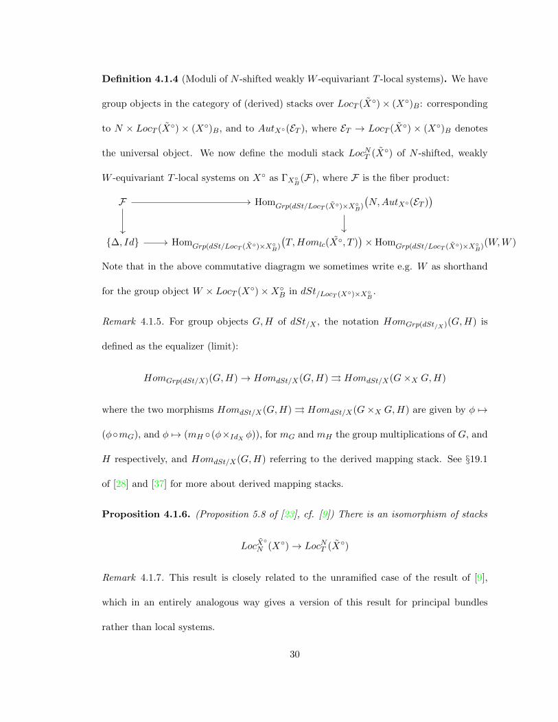
Definition 4.1.4 (Moduli of N -shifted weakly W -equivariant T -local systems). We have
group objects in the category of (derived) stacks over LocT (X◦)× (X◦)B: corresponding
to N × LocT (X◦) × (X◦)B, and to AutX◦(ET ), where ET → LocT (X
◦) × (X◦)B denotes
the universal object. We now define the moduli stack LocNT (X◦) of N -shifted, weakly
W -equivariant T -local systems on X◦ as ΓX◦B(F), where F is the fiber product:
F HomGrp(dSt/LocT (X◦)×X◦B)
�N,AutX◦(ET )
�
{Δ, Id} HomGrp(dSt/LocT (X◦)×X◦B)
�T,Homlc(X◦, T )
�×HomGrp(dSt/LocT (X◦)×X◦
B)(W,W )
Note that in the above commutative diagragm we sometimes write e.g. W as shorthand
for the group object W × LocT (X◦)×X◦
B in dSt/LocT (X◦)×X◦B.
Remark 4.1.5. For group objects G,H of dSt/X , the notation HomGrp(dSt/X)(G,H) is
defined as the equalizer (limit):
HomGrp(dSt/X)(G,H) → HomdSt/X(G,H) ⇒ HomdSt/X(G×X G,H)
where the two morphisms HomdSt/X(G,H) ⇒ HomdSt/X(G×X G,H) are given by φ �→
(φ◦mG), and φ �→ (mH ◦ (φ×IdX φ)), for mG and mH the group multiplications of G, and
H respectively, and HomdSt/X(G,H) referring to the derived mapping stack. See §19.1
of [28] and [37] for more about derived mapping stacks.
Proposition 4.1.6. (Proposition 5.8 of [23], cf. [9]) There is an isomorphism of stacks
LocX◦
N (X◦) → LocNT (X◦)
Remark 4.1.7. This result is closely related to the unramified case of the result of [9],
which in an entirely analogous way gives a version of this result for principal bundles
rather than local systems.
30
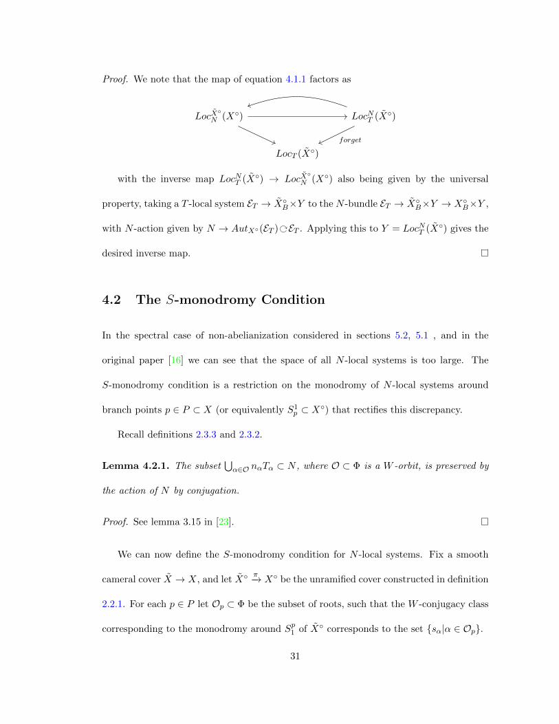
Proof. We note that the map of equation 4.1.1 factors as
LocX◦
N (X◦) LocNT (X◦)
LocT (X◦)
forget
with the inverse map LocNT (X◦) → LocX◦
N (X◦) also being given by the universal
property, taking a T -local system ET → X◦B×Y to the N -bundle ET → X◦
B×Y → X◦B×Y ,
with N -action given by N → AutX◦(ET )
� ET . Applying this to Y = LocNT (X◦) gives the
desired inverse map.
4.2 The S-monodromy Condition
In the spectral case of non-abelianization considered in sections 5.2, 5.1 , and in the
original paper [16] we can see that the space of all N -local systems is too large. The
S-monodromy condition is a restriction on the monodromy of N -local systems around
branch points p ∈ P ⊂ X (or equivalently S1p ⊂ X◦) that rectifies this discrepancy.
Recall definitions 2.3.3 and 2.3.2.
Lemma 4.2.1. The subset�
α∈O nαTα ⊂ N , where O ⊂ Φ is a W -orbit, is preserved by
the action of N by conjugation.
Proof. See lemma 3.15 in [23].
We can now define the S-monodromy condition for N -local systems. Fix a smooth
cameral cover X → X, and let X◦ π−→ X◦ be the unramified cover constructed in definition
2.2.1. For each p ∈ P let Op ⊂ Φ be the subset of roots, such that the W -conjugacy class
corresponding to the monodromy around Sp1 of X◦ corresponds to the set {sα|α ∈ Op}.
31
We then define:
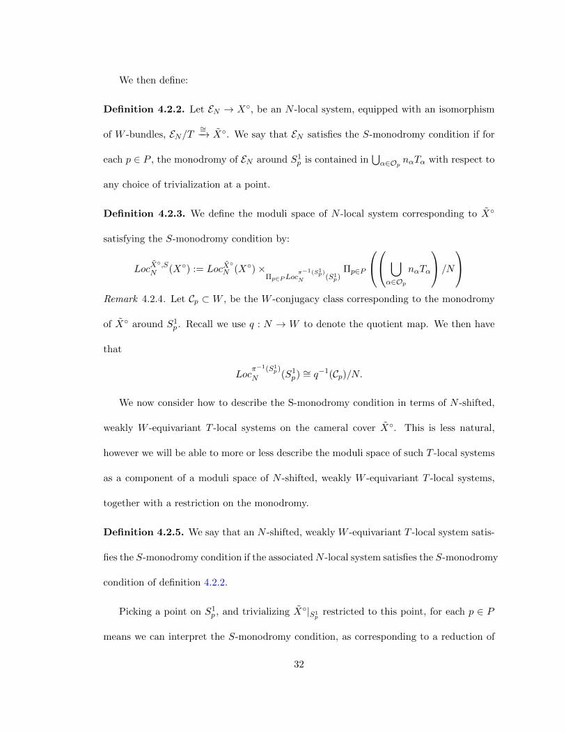
Definition 4.2.2. Let EN → X◦, be an N -local system, equipped with an isomorphism
of W -bundles, EN/T∼=−→ X◦. We say that EN satisfies the S-monodromy condition if for
each p ∈ P , the monodromy of EN around S1p is contained in
�α∈Op
nαTα with respect to
any choice of trivialization at a point.
Definition 4.2.3. We define the moduli space of N -local system corresponding to X◦
satisfying the S-monodromy condition by:
LocX◦,S
N (X◦) := LocX◦
N (X◦)×Πp∈PLoc
π−1(S1p)
N (S1p)Πp∈P
�
α∈Op
nαTα
/N
Remark 4.2.4. Let Cp ⊂ W , be the W -conjugacy class corresponding to the monodromy
of X◦ around S1p . Recall we use q : N → W to denote the quotient map. We then have
that
Locπ−1(S1
p)
N (S1p)
∼= q−1(Cp)/N.
We now consider how to describe the S-monodromy condition in terms of N -shifted,
weakly W -equivariant T -local systems on the cameral cover X◦. This is less natural,
however we will be able to more or less describe the moduli space of such T -local systems
as a component of a moduli space of N -shifted, weakly W -equivariant T -local systems,
together with a restriction on the monodromy.
Definition 4.2.5. We say that an N -shifted, weakly W -equivariant T -local system satis-
fies the S-monodromy condition if the associatedN -local system satisfies the S-monodromy
condition of definition 4.2.2.
Picking a point on S1p , and trivializing X◦|S1
prestricted to this point, for each p ∈ P
means we can interpret the S-monodromy condition, as corresponding to a reduction of
32
structure of theN -local system on S1p to SL2, with respect to the morphism Iα : SL2 → G,
where α is the root, such that sα is the monodromy of X◦|S1p.
For SL2, noting that W ∼= {1, s}, and that for any n ∈ q−1(s), we have n2 = −Id, we
have that in the caseG = SL(2), anN -local system satisfying the S-monodromy condition
is mapped under the map of proposition 4.1.6 to an N -shifted, weakly W -equivariant T -
local system with the property that the monodromy around S1r is Iα(r)(−Id) for each
r ∈ R, where α(r) is one of the two roots such that X intersects the hyperplane Hα at r.
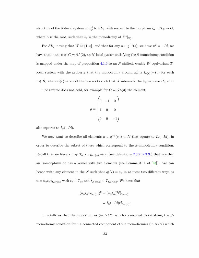
The reverse does not hold, for example for G = GL(3) the element
g =
0 −1 0
1 0 0
0 0 −1
also squares to Iα(−Id).
We now want to describe all elements n ∈ q−1(sα) ⊂ N that square to Iα(−Id), in
order to describe the subset of these which correspond to the S-monodromy condition.
Recall that we have a map Tα × TKer(α) → T (see definitions 2.3.2, 2.3.3 ) that is either
an isomorphism or has a kernel with two elements (see Lemma 3.11 of [23]). We can
hence write any element in the N such that q(N) = sα in at most two different ways as
n = nαtαtKer(α) with tα ∈ Tα, and tKer(α) ∈ TKer(α). We have that
(nαtαtKer(α))2 = (nαtα)
2t2Ker(α)
= Iα(−Id)t2Ker(α).
This tells us that the monodromies (in N/N) which correspond to satisfying the S-
monodromy condition form a connected component of the monodromies (in N/N) which
33
upon choosing a trivialization of the cameral cover to reduce from N/N to N/T square
to an element Iα(−Id) for α ∈ Op.
Note that for deg(D) > 0 we have that LocXN (X) is connected (as the character variety
is connected because D is non-zero). Furthermore it is clear that LocX,SN (X) is connected.
We can hence make the following definition:
Definition 4.2.6. We define the moduli stack of N -shifted, weakly W -equivariant T -
bundles on X◦ as the connected component of
LocNT (X◦)×LocT (�
r∈R(S1r ))
Πr∈R{−Id},
containing the image of LocX,SN (X).
Because nαTα is a connected component of the stack q−1(sα) ×T {−Id}, where the
map q−1(sα) → T is n �→ n2, we gain the following theorem.
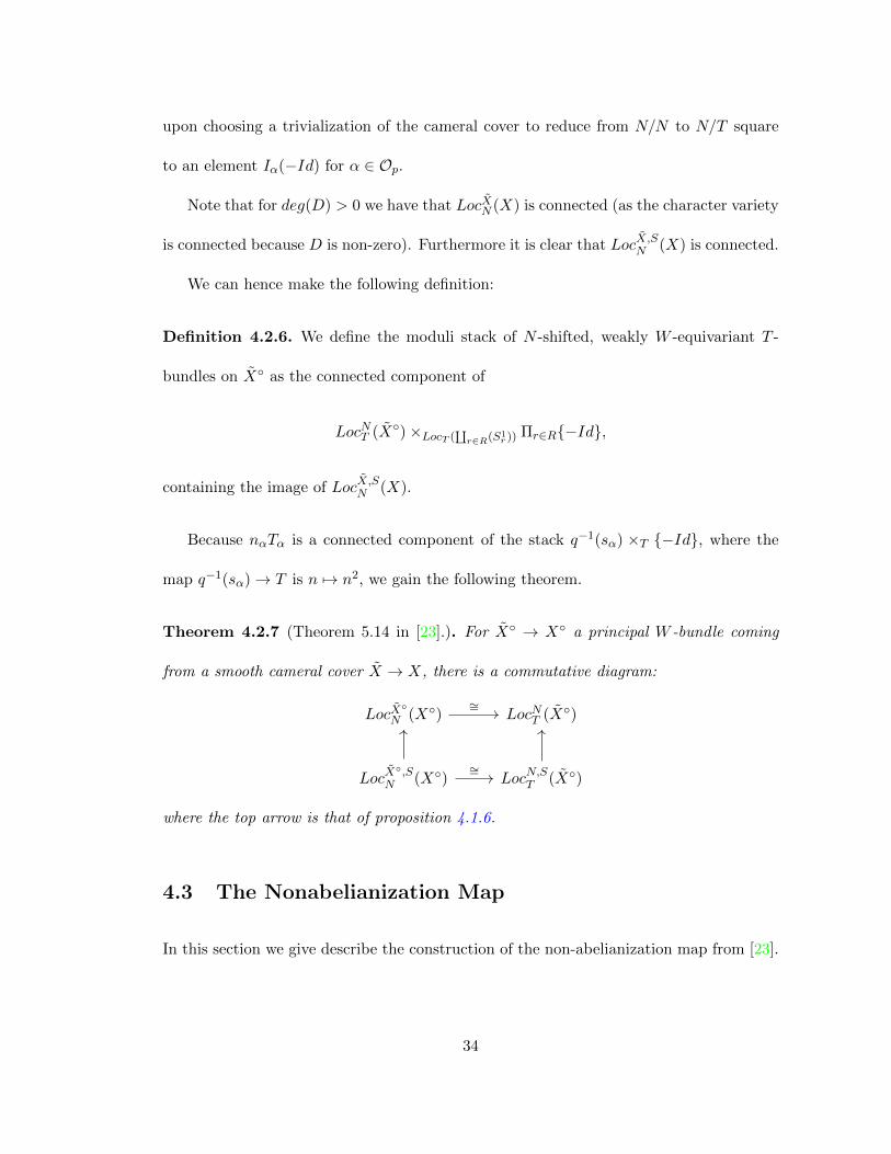
Theorem 4.2.7 (Theorem 5.14 in [23].). For X◦ → X◦ a principal W -bundle coming
from a smooth cameral cover X → X, there is a commutative diagram:
LocX◦
N (X◦) LocNT (X◦)
LocX◦,S
N (X◦) LocN,ST (X◦)
∼=
∼=
where the top arrow is that of proposition 4.1.6.
4.3 The Nonabelianization Map
In this section we give describe the construction of the non-abelianization map from [23].
34
By definition 3.2.5 we have a filtration FiW of the connected components ofW\J , with
the property that F0W is the union of the lines emerging from branch points p ∈ P ⊂ X
(or strictly speaking from the associated boundary circles S1p) as shown in lemma 3.2.4.
The large scale structure of the non-abelianization construction can be seen as fol-
lows. We are going to “cut and reglue” a G local system induced from any given N -local
system, corresponding to X◦ satisfying the S-monodromy condition, along the locus W.
To do this we need to produce automorphisms of the G local system restricted to each
connected component of W\J . We will call these automorphisms Stokes factors. We
do this inductively using the filtration F•W. We then define the reglue map (for speci-
fied automorphisms) in construction 4.3.9, which describes “cutting” along W and then
“regluing” by specified automorphisms.
We first define some moduli stacks that parameterize appropriate N -local systems EN ,
together with certain automorphisms of the induced G-local system EG := EN ×N G. Note
that inducing a G-local system provides a map LocN (X◦) → LocG(X◦), which given the
mapping stack description LocN (X◦) = Map(X◦, BN), corresponds to postcomposing a
map with the map BN → BG induced from the inclusion N �→ G.
We first give a definition of the moduli of G-local systems on X◦ equipped with
automorphisms of the local system restricted to a set of lines1. Firstly note that the
universal bundle pt → BG has the sheaf of automorphisms G/G → BG. Hence we make
the following definition:
1By lines we mean one dimensional topological submanifolds of the topological manifold X◦.
35
Definition 4.3.1. For FiW\J =�
j �j for disjoint line segments �j we define
AutFiWG (X◦�) := LocG(X
◦�)×LocG(�
j �j)Hom(
�
j
(�j)B, G/G).
Similarly for W\J =�
j �j for disjoint line segments �j we define
AutWG (X◦�) := LocG(X◦�)×LocG(
�j �j)
Hom(�
j
(�j)B, G/G).
Definition 4.3.2. We define
AutFiW,X◦�(X◦�) := LocX
◦� ,SN (X◦�)×LocG(X◦� ) Aut
FiWG (X◦�),
where the map LocX◦� ,S
N (X◦�) → LocG(X◦�) is the composition of the forgetful map, with
the map coming from inducing from N -local systems to G-local systems;
LocX◦� ,S
N (X◦�)forget−−−−→ LocN (X◦�) → LocG(X
◦�).
Definition 4.3.3. Similarly we define
AutW,X◦�(X◦�) := LocX
◦� ,SN (X◦�)×LocG(X◦� ) Aut
WG (X◦�).
Note that for N sufficiently large we have AutFNW,X◦�(X◦�) = AutW,X◦�
(X◦�).
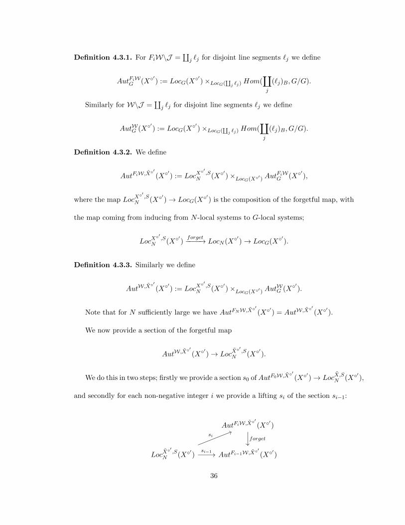
We now provide a section of the forgetful map
AutW,X◦�(X◦�) → LocX
◦� ,SN (X◦�).
We do this in two steps; firstly we provide a section s0 ofAutF0W,X◦�
(X◦�) → LocX,SN (X◦�),
and secondly for each non-negative integer i we provide a lifting si of the section si−1:
AutFiW,X◦�(X◦�)
LocX◦� ,S
N (X◦�) AutFi−1W,X◦�(X◦�)
forgetsi
si−1
36
Noting that for N sufficiently large we have AutFNW,X◦�(X◦�) = AutW,X◦�
(X◦�), com-
posing the sections obtained above gives a section we denote sWKB of the forgetful map
AutW,X◦�(X◦�) LocX
◦� ,SN (X◦�).
forget
sWKB
(4.3.1)
4.3.1 Stokes Factors for Initial Stokes Lines
We will being by giving a very explicit calculation for G = SL2. We note that for simply
laced groups with a faithful miniscule representation, the path detour rules explained in
section 5.2 provide an alternative construction.
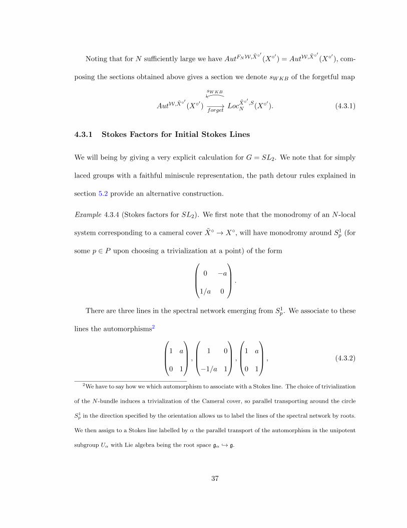
Example 4.3.4 (Stokes factors for SL2). We first note that the monodromy of an N -local
system corresponding to a cameral cover X◦ → X◦, will have monodromy around S1p (for
some p ∈ P upon choosing a trivialization at a point) of the form
0 −a
1/a 0
.
There are three lines in the spectral network emerging from S1p . We associate to these
lines the automorphisms2
1 a
0 1
,
1 0
−1/a 1
,
1 a
0 1
, (4.3.2)
2We have to say how we which automorphism to associate with a Stokes line. The choice of trivialization
of the N -bundle induces a trivialization of the Cameral cover, so parallel transporting around the circle
S1p in the direction specified by the orientation allows us to label the lines of the spectral network by roots.
We then assign to a Stokes line labelled by α the parallel transport of the automorphism in the unipotent
subgroup Uα with Lie algebra being the root space gα �→ g.
37
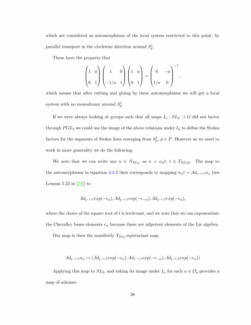
which are considered as automorphisms of the local system restricted to this point, by
parallel transport in the clockwise direction around S1p .
These have the property that
1 a
0 1
1 0
−1/a 1
1 a
0 1
=
0 −a
1/a 0
−1
,
which means that after cutting and gluing by these automorphisms we will get a local
system with no monodromy around S1p .
If we were always looking at groups such that all maps Iα : SL2 → G did not factor
through PGL2 we could use the image of the above relations under Iα to define the Stokes
factors for the segments of Stokes lines emerging from S1p , p ∈ P . However as we need to
work in more generality we do the following:
We note that we can write any n ∈ NSL2 , as n = nαt, t ∈ TSL(2). The map to
the automorphisms in equation 4.3.2 then corresponds to mapping nαt = Adt−1/2nα (see
Lemma 5.22 in [23]) to
Adt−1/2exp(−eα), Adt−1/2exp(−e−α), Adt−1/2exp(−eα),
where the choice of the square root of t is irrelevant, and we note that we can exponentiate
the Chevalley bases elements eα because these are nilpotent elements of the Lie algebra.
Our map is then the manifestly TSL2-equivariant map
Adt−1/2nα �→ (Adt−1/2exp(−eα), Adt−1/2exp(−e−α), Adt−1/2exp(−eα))
Applying this map to SL2, and taking its image under Iα for each α ∈ Op provides a
map of schemes
38
�
α∈Op
nαTα →�
α∈Op
Uα × U−α × Uα.
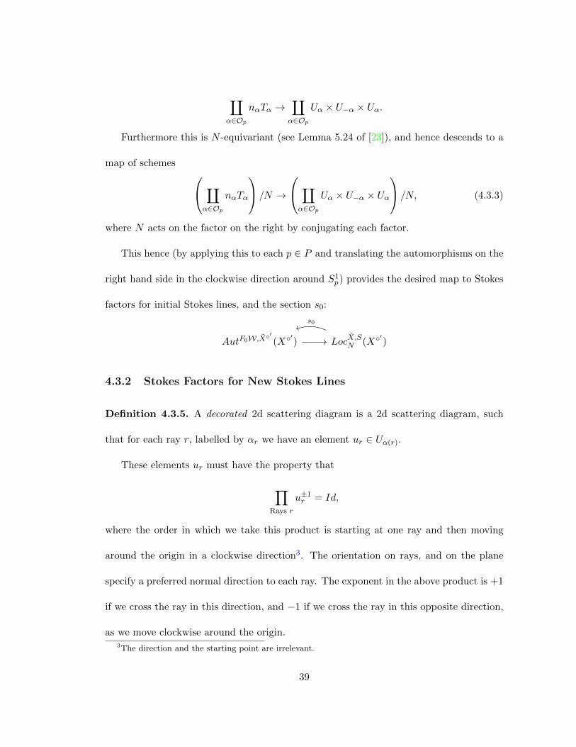
Furthermore this is N -equivariant (see Lemma 5.24 of [23]), and hence descends to a
map of schemes �
α∈Op
nαTα
/N →
�
α∈Op
Uα × U−α × Uα
/N, (4.3.3)
where N acts on the factor on the right by conjugating each factor.
This hence (by applying this to each p ∈ P and translating the automorphisms on the
right hand side in the clockwise direction around S1p) provides the desired map to Stokes
factors for initial Stokes lines, and the section s0:
AutF0W,X◦�(X◦�) LocX,S
N (X◦�)
s0
4.3.2 Stokes Factors for New Stokes Lines
Definition 4.3.5. A decorated 2d scattering diagram is a 2d scattering diagram, such
that for each ray r, labelled by αr we have an element ur ∈ Uα(r).
These elements ur must have the property that
�
Rays r
u±1r = Id,
where the order in which we take this product is starting at one ray and then moving
around the origin in a clockwise direction3. The orientation on rays, and on the plane
specify a preferred normal direction to each ray. The exponent in the above product is +1
if we cross the ray in this direction, and −1 if we cross the ray in this opposite direction,
as we move clockwise around the origin.3The direction and the starting point are irrelevant.
39
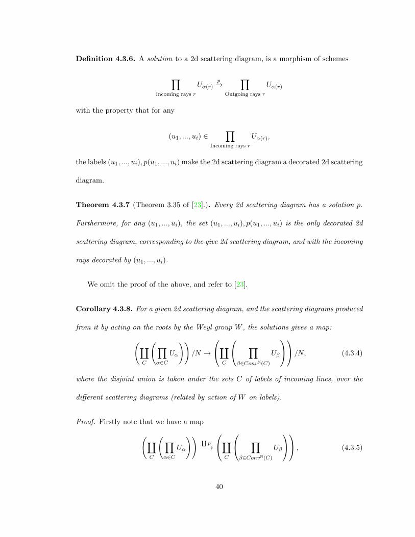
Definition 4.3.6. A solution to a 2d scattering diagram, is a morphism of schemes
�
Incoming rays r
Uα(r)p−→
�
Outgoing rays r
Uα(r)
with the property that for any
(u1, ..., ui) ∈�
Incoming rays r
Uα(r),
the labels (u1, ..., ui), p(u1, ..., ui) make the 2d scattering diagram a decorated 2d scattering
diagram.
Theorem 4.3.7 (Theorem 3.35 of [23].). Every 2d scattering diagram has a solution p.
Furthermore, for any (u1, ..., ui), the set (u1, ..., ui), p(u1, ..., ui) is the only decorated 2d
scattering diagram, corresponding to the give 2d scattering diagram, and with the incoming
rays decorated by (u1, ..., ui).
We omit the proof of the above, and refer to [23].
Corollary 4.3.8. For a given 2d scattering diagram, and the scattering diagrams produced
from it by acting on the roots by the Weyl group W , the solutions gives a map:
��
C
��
α∈CUα
��/N →
�
C
�
β∈ConvN(C)
Uβ
/N, (4.3.4)
where the disjoint union is taken under the sets C of labels of incoming lines, over the
different scattering diagrams (related by action of W on labels).
Proof. Firstly note that we have a map
��
C
��
α∈CUα
�� �p−−→
�
C
�
β∈ConvN(C)
Uβ
, (4.3.5)
40
given by the solutions to the 2d scattering diagrams. The N -equivariance follows from
the uniqueness statement of Theorem 4.3.7, because if n ∈ N with q(n) = w ∈ W , and
(u1, ..., ui, ui+1, ..., ui+j) is a decoration of a scattering diagram, then
(nu1n−1, ..., nuin
−1, nui+1n−1, ..., nui+jn
−1)
is a decoration of the scattering diagram obtained by acting on all labels of rays by w.
Hence if we denote p1 the solution to the first scattering diagram, and p2 the solution
to the second, we have that
np1(u1, ..., ui)n−1 = p2(nu1n
−1, ..., nuin−1),
where by np1(u1, ..., ui)n−1 we mean acting by conjugation on each of the factors Uβ ,
β ∈ ConvN(C).
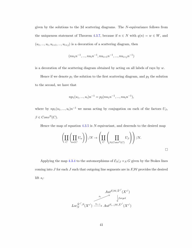
Hence the map of equation 4.3.5 is N -equivariant, and descends to the desired map
��
C
��
α∈CUα
��/N →
�
C
�
β∈ConvN(C)
Uβ
/N.
Applying the map 4.3.4 to the automorphisms of EN |J ×N G given by the Stokes lines
coming into J for each J such that outgoing line segments are in FiW provides the desired
lift si:
AutFiW,X◦�(X◦�)
LocX◦� ,S
N (X◦�) AutFi−1W,X◦�(X◦�)
forgetsi
si−1
41
4.3.3 Reglue Map
We now describe the regluing map, which corresponds to “cutting and regluing” a given
G-local system along certain lines, using specified automorphisms of the G-local system.
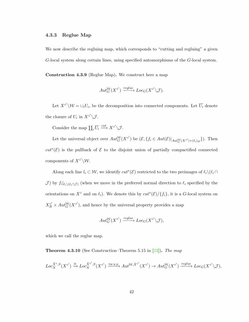
Construction 4.3.9 (Reglue Map). We construct here a map
AutWG (X◦�)reglue−−−−→ LocG(X
◦�\J ).
Let X◦�\W = ∪iUi, be the decomposition into connected components. Let Ui denote
the closure of Ui in X◦�\J .
Consider the map�
i Uicut−−→ X◦�\J .
Let the universal object over AutWG (X◦�) be (E , {fi ∈ Aut(E)|AutWG (X◦� )×(�i)B}). Then
cut∗(E) is the pullback of E to the disjoint union of partially compactified connected
components of X◦�\W.
Along each line li ⊂ W, we identify cut∗(E) restricted to the two preimages of �i\(�i ∩
J ) by fi|�i\(�i∩J ) (when we move in the preferred normal direction to �i specified by the
orientations on X◦ and on �i). We denote this by cut∗(E)/{fi}, it is a G-local system on
X◦�B ×AutWG (X◦�), and hence by the universal property provides a map
AutWG (X◦�)reglue−−−−→ LocG(X
◦�\J ),
which we call the reglue map.
Theorem 4.3.10 (See Construction–Theorem 5.15 in [23]). The map
LocX◦,S
N (X◦�)∼=−→ LocX
◦� ,SN (X◦�)
sWKB−−−−→ AutW,X◦�(X◦�) → AutWG (X◦�)
reglue−−−−→ LocG(X◦�\J ),
42
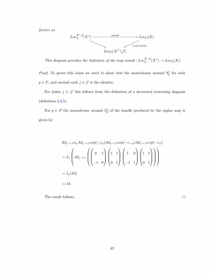
factors as
LocX◦,S
N (X◦) LocG(X)
LocG(X◦�\J )
nonab
restriction
This diagram provides the definition of the map nonab : LocX◦,S
N (X◦) → LocG(X).
Proof. To prove this claim we need to show that the monodromy around S1p for each
p ∈ P , and around each j ∈ J is the identity.
For joints j ∈ J this follows from the definition of a decorated scattering diagram
(definition 4.3.5).
For p ∈ P the monodromy around S1p of the bundle produced by the reglue map is
given by
Adt−1/2nαAdt−1/2exp(−eα)Adt−1/2exp(−e−α)Adt−1/2exp(−eα)
= Iα
Adt−1/2
0 1
−1 0
1 1
0 1
1 0
−1 1
1 1
0 1
= Iα(Id)
= Id.
The result follows.
43
Chapter 5
Spectral Descriptions of
Nonabelianization
5.1 Spectral and Cameral Covers
Let X → X be a cameral cover. We will give alternative descriptions of the data provided
by these, and of the N -bundles corresponding to these in terms of spectral covers, and local
systems of vector spaces on these. This is the ahistorical direction: Spectral covers were
introduced in [20] to describe fibers of the Hitchin moduli space for classical groups. See
[4, 31] for further results in this direction for G = GL(n). Cameral covers were introduced
in [10, 32, 8] as a replacement of spectral covers for arbitrary reductive algebraic groups
G. In [9] the Hitchin fiber for a smooth cameral cover is described in terms of N -shifted,
weakly W -equivariant T -bundles on the cameral cover. Some results on the relation
between descriptions of Hitchin fibers using cameral and spectral covers are found in [8],
and for GL(n) the precise relation for the regular part of Hitchin fibers is found in [9]. In
44
this section we are using the unramified cameral cover X◦ → X◦, and as such don’t need
to engage with the difficult question of what happens at ramification points, and instead
only need to provide a description of the S-monodromy condition in terms of the local
systems on the spectral covers.
5.1.1 Constructing Spectral Covers from Cameral Covers
Construction 5.1.1 (Spectral covers from unramified Cameral covers.). We work with
a fixed reductive algebraic group G with maximal torus T , and with a cameral cover
X → X.
Let ρ : G → GL(V ) be a representation, with weights Ωρ.
We define the non-embedded spectral cover associated to ρ as
Xneρ := X ×W Ωρ. (5.1.1)
Note that this is equipped with a map π : Xneρ → X
We denote by Rρ ⊂ Xneρ the ramification divisor. We retain P to denote the branch
locus of X → X. Note that the branch locus of Xneρ is a subdivisor of P .
We also define the real blow up
Xne,◦Pρ := ReBlπ−1(P )(X
neρ ). (5.1.2)
Note that Xne,◦Pρ
∼= X ×W Ωρ.
Finally we define
Xne,◦Rρ := ReBlπ−1(Rρ)(X
neρ ). (5.1.3)
We also introduce the following variant:
45
Pick decomposition of the induced representation of the normalizer N �→ T , as ρ|N =
⊕iρi where the weight spaces of each ρi are one dimensional. Let Ωρi be the weights of ρi.
Note that there always exists such a decomposition; one can be constructed by taking the
weight space decomposition of ρ, and then for one weight in each W -orbit of the weights,
we pick a basis of the weight space. We then take the ρi to be the representation of N
corresponding to the vector subspace of V spanned by the N -orbit of one of the basis
elements.
Definition 5.1.2. Let G, T , X → X, ρ, ρ|N = ⊕iρi be as above.
We then define:
Xne,rρ :=
�
i
X ×W Ωρi .
We again use Rρ ⊂ Xne,rρ to denote the ramification divisor, we hope this does not
cause confusion.
As in the preceding case we also define the real blow ups:
Xne,r,◦Pρ := ReBlπ−1(P )(X
ne,rρ ), (5.1.4)
and
Xne,r,◦Rρ := ReBlπ−1(Rρ)(X
ne,rρ ). (5.1.5)
5.1.2 Local systems on Spectral covers from N-local systems
In this section we describe how to construct local systems of vector spaces on spectral
covers from N -local systems corresponding to a given cameral cover. We also consider
how imposing the S-monodromy condition affects which local systems we produce.
46
Construction 5.1.3. We fix T , G, X → X, and ρ as before.
Let EN → X◦ be an N -bundle on X◦, equipped with an isomorphism EN/T∼=−→ X◦ as
W -bundles.
Let V = ⊕ω∈ΩρVω be the decomposition of V as a direct sum of weight spaces Vω of
T .
Define
L := EN ×N
�
ω∈Ωρ
Vω
.
Note that the map��
ω∈ΩρVω
�→ Ωρ, which maps the weight space Vω to the point
ω provides a map
L → Xne,◦Pρ .
This realizes L as a local system of vector spaces on Xne,◦Pρ .
Applying this to the universal bundle, and applying the universal property this pro-
vides a map:
LocX◦
N (X◦) → LocV ect(Xne,◦Pρ ),
where LocV ect(Xne,◦Pρ ) is the indstack of local systems of vector bundles on X
ne,◦Pρ .
We provide also the following variant:
Construction 5.1.4. We fix T , G, X → X, and ρ as before, together with a decompo-
sition ρ|N = ⊕iρi as in section 5.1.1.
Applying construction 5.1.3 to each representation ρi, noting that we actually only
require an N -representation rather than a G representation in this construction, provides
a map which we denote Spρ:
47
LocX◦
N (X◦)Spρ−−→ LocGm(X
ne,r,◦Pρ ),
where we are using the equivalence between local systems of one dimensional vector spaces
and Gm local systems.
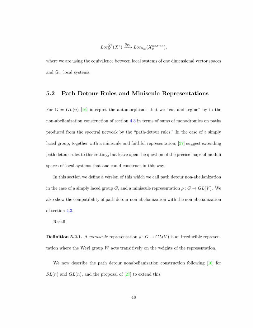
5.2 Path Detour Rules and Miniscule Representations
For G = GL(n) [16] interpret the automorphisms that we “cut and reglue” by in the
non-abelianization construction of section 4.3 in terms of sums of monodromies on paths
produced from the spectral network by the “path-detour rules.” In the case of a simply
laced group, together with a miniscule and faithful representation, [27] suggest extending
path detour rules to this setting, but leave open the question of the precise maps of moduli
spaces of local systems that one could construct in this way.
In this section we define a version of this which we call path detour non-abelianization
in the case of a simply laced group G, and a miniscule representation ρ : G → GL(V ). We
also show the compatibility of path detour non-abelianization with the non-abelianization
of section 4.3.
Recall:
Definition 5.2.1. A miniscule representation ρ : G → GL(V ) is an irreducible represen-
tation where the Weyl group W acts transitively on the weights of the representation.
We now describe the path detour nonabelianization construction following [16] for
SL(n) and GL(n), and the proposal of [27] to extend this.
48
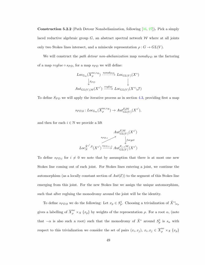
Construction 5.2.2 (Path Detour Nonabelianization, following [16, 27]). Pick a simply
laced reductive algebraic group G, an abstract spectral network W where at all joints
only two Stokes lines intersect, and a miniscule representation ρ : G → GL(V ).
We will construct the path detour non-abelianization map nonabPD as the factoring
of a map reglue ◦ sPD, for a map sPD we will define:
LocGm(Xne,◦Rρ ) LocGL(V )(X
◦)
AutGL(V ),W(X◦�) LocGL(V )(X◦\J )
SPD
nonabPD
reglue
To define SPD we will apply the iterative process as in section 4.3, providing first a map
sPD,0 : LocGm(Xne,◦Rρ ) → AutF0W
GL(V )(X◦�),
and then for each i ∈ N we provide a lift
AutFiWGL(V )(X
◦�)
LocX◦� ,S
N (X◦�) AutFi−1WGL(V ) (X
◦�)
forgetsPD,i
sPD,i−1
To define sPD,i for i �= 0 we note that by assumption that there is at most one new
Stokes line coming out of each joint. For Stokes lines entering a joint, we continue the
automorphism (as a locally constant section of Aut(E)) to the segment of this Stokes line
emerging from this joint. For the new Stokes line we assign the unique automorphism,
such that after regluing the monodromy around the joint will be the identity.
To define sPD,0 we do the following: Let xp ∈ S1p . Choosing a trivialization of X◦|xp
gives a labelling of Xneρ ×X {xp} by weights of the representation ρ. For a root α, (note
that −α is also such a root) such that the monodromy of X◦ around S1p is sα with
respect to this trivialization we consider the set of pairs (xi, xj), xi, xj ∈ Xneρ ×X {xp}
49
with the property that l(xi) − l(xj) = α, where l(xm) refers to the weight labelling the
branch xm is on, with respect to the chosen trivialization. Note that the set of pairs of
Xneρ ×X {xp} is independent of the choice of trivialization because if l(xi) − l(xj) = α,
then w(l(xi))− w(l(xj)) = w(α).
To a line bundle L on Xne,◦Rρ , we define E := π∗L. We define dxi,xj to be the parallel
transport in L attached to the lift starting at xi of the path γp going around p in the
opposition orientation to that of S1p .
To a Stokes line emitted from S1p , which is labelled by α with respect to the choice of
trivialization of X◦, we let
Sdetour := exp��
dxi,xj
�∈ GL(E|xs),
(using dxi,xj for the choice of root α).
Doing this in families, for each initial Stokes line provides the section
sPD,0 : LocGm(Xne,◦Rρ ) → AutF0W
GL(V )(X◦�),
together with the specified lifts sPD,i this specifies the map sPD as the composition:
LocGm(Xne,◦Rρ ) AutFNW
GL(V )(X◦�) AutWGL(V )(X
◦�).
sPD
sPD,N ∼=
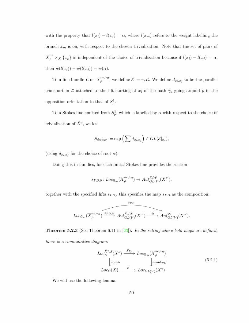
Theorem 5.2.3 (See Theorem 6.11 in [23]). In the setting where both maps are defined,
there is a commutative diagram:
LocX◦,S
N (X◦) LocGm(Xne,◦Rρ )
LocG(X) LocGL(V )(X◦)
Spρ
nonab nonabPD
ρ
(5.2.1)
We will use the following lemma:
50
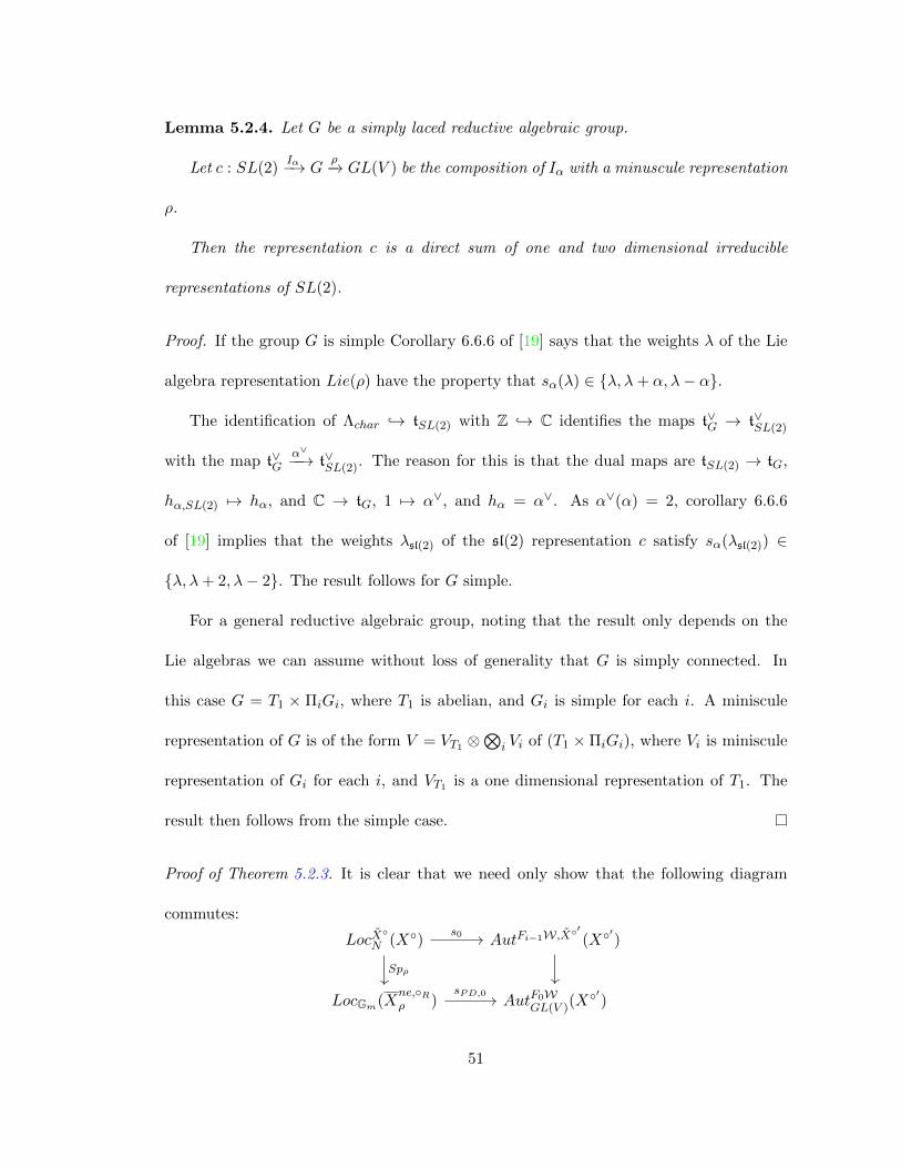
Lemma 5.2.4. Let G be a simply laced reductive algebraic group.
Let c : SL(2)Iα−→ G
ρ−→ GL(V ) be the composition of Iα with a minuscule representation
ρ.
Then the representation c is a direct sum of one and two dimensional irreducible
representations of SL(2).
Proof. If the group G is simple Corollary 6.6.6 of [19] says that the weights λ of the Lie
algebra representation Lie(ρ) have the property that sα(λ) ∈ {λ,λ+ α,λ− α}.
The identification of Λchar �→ tSL(2) with Z �→ C identifies the maps t∨G → t∨SL(2)
with the map t∨Gα∨−−→ t∨SL(2). The reason for this is that the dual maps are tSL(2) → tG,
hα,SL(2) �→ hα, and C → tG, 1 �→ α∨, and hα = α∨. As α∨(α) = 2, corollary 6.6.6
of [19] implies that the weights λsl(2) of the sl(2) representation c satisfy sα(λsl(2)) ∈
{λ,λ+ 2,λ− 2}. The result follows for G simple.
For a general reductive algebraic group, noting that the result only depends on the
Lie algebras we can assume without loss of generality that G is simply connected. In
this case G = T1 × ΠiGi, where T1 is abelian, and Gi is simple for each i. A miniscule
representation of G is of the form V = VT1 ⊗�
i Vi of (T1 ×ΠiGi), where Vi is miniscule
representation of Gi for each i, and VT1 is a one dimensional representation of T1. The
result then follows from the simple case.
Proof of Theorem 5.2.3. It is clear that we need only show that the following diagram
commutes:
LocX◦
N (X◦) AutFi−1W,X◦�(X◦�)
LocGm(Xne,◦Rρ ) AutF0W
GL(V )(X◦�)
s0
Spρ
sPD,0
51
where the map on the right hand side of the above commutative square is the composition
AutFi−1W,X◦�(X◦�) → AutF0W
G (X◦�) → AutF0WGL(V )(X
◦�).
We pick a trivialization of the an N -bundle corresponding to X◦� at xp ∈ S1p ⊂ X◦� ,
such that the monodromy around S1p (in the direction specified by the orientation of S1
p)
is nα. We then have that the monodromy around the path γp in construction 5.2.2 is
ρ(n−1α ). By lemma 5.2.4 we have that
ρ(n−1α ) = ρ(−eα) + ρ(−e−α) + Id⊕ω|ω(α)=0Vω ,
which gives the identification ρ(−eα) =�
di,j .
We hence have that the Stokes factor assigned by sPD,0 to a line labelled by α with
respect to the chosen trivialization at xp is given by sPD = exp(�
di,j) = exp(ρ(−eα)) =
ρ(exp(−eα)). The case of lines labelled by −α is analogous.
5.3 Spectral Description of N-Local Systems For Classical
Groups
In this section we describe the relation between the moduli of N -local systems correspond-
ing to a given cameral cover (satisfying the S-monodromy condition) and certain moduli
spaces of Gm-local systems on spectral covers. These results appear in §6.4 of [23].
52
5.3.1 The Case of GL(n), and SL(n)
Firstly we note that for GL(n) we can describe the Hitchin base, associated to Xc and
the line bundle KXc(D) as
⊕ni=1Γ(X, (KXc(D))⊗i) ∼= Γ(Xc, tGL(n),KXc (D)/W ),
by using the basis of C[t]W given by the elementary symmetric polynomials. Specifically
the ith elementary symmetric polynomial gives a map tKXc (D)/W → K⊗iXc(D).
For G = SL(n) we have a basis of C[t]W , corresponding under the inclusion tSL(n) →
tGL(n) to the elementary symmetric polynomials with the exception of the trace.
We hence have an isomorphism
⊕ni=2Γ(X, (KXc(D))⊗i) ∼= Γ(Xc, tSL(n),KXc (D)/W ).
Given a point in the GL(n) Hitchin base, potentially one corresponding to a point in
the SL(n) Hitchin base we can define the spectral curve as follows:
Definition 5.3.1. The spectral cover Xcassociated to (a1, ..., an) ∈ ⊕n
i=1Γ(X, (KXc(D))⊗i)
is the locus in Tot(KXc(D)) where the section
Σni=0(−1)n−iλn−iai
(which we call the characteristic polynomial) of p∗(KXc(D))⊗n intersects the zero section.
Here p denotes the map p : Tot(KXc(D)) → Xc, and λ is the tautological section of
p∗(KXc(D)).
This is equipped with the map π = p|Xc : Xc → Xc.
We denote X := Xc ×Xc X. We denote X
◦R := ReBlR(X) the real blow up along
the ramification locus R ⊂ X of X → X. We denote by X◦P := ReBlP (X) the real blow
53
of X up along the preimage π−1(P ) of the branch locus P of X → X along the map
π : X → X.
Proposition 5.3.2. For G = GL(n) or G = SL(n), and a ∈ A♦ there is an isomor-
phism of schemes Xneρ
∼= X between the non-embedded spectral cover for ρ the defining
representation, and the spectral cover.
Proof. Choose an identification t ∼= Cn, that identifies W with Sn acting by permuting
the copies of C. A projection t ∼= Cn → C to one of these copies of C provides a map
tKXc (D) → Tot(KXc(D)) that maps X → X. This factors through the map Xneρ , giving
an isomorphism Xneρ
∼= X.
Proposition 5.3.3 (Spectral and Cameral descriptions of local systems for Gl(n) without
S-monodromy condition, cf. [9]). For G = GL(n) there is an isomorphism of stacks
LocGm(X◦P ) → LocX
◦N (X◦P )
Proof. Note that for each i ∈ {1, ..., n} we have an inclusion Sn−1 �→ Sn. Let πi : X → X
be the map coming from quotienting by Sn−1, or equivalently in the proof of 5.3.2 comes
from projecting onto the ith copy of C.
Let L ∈ LocGm(X◦P ), and ET ∈ LocX
◦N (X◦P ). We have inverse maps given by
L �→ ⊕ni=1π
∗iL,
and construction 5.1.4.
Note that to realize ⊕π∗iL as an N -local system we are using proposition 4.1.6, and
that as for GL(n) the sequence 1 → T → N → W → 1 splits, an N -shifted weakly
54
W -equivariant T -bundle on X◦ is equivalent to a W -equivariant T bundle on X◦, which
is what ⊕π∗iL is.
Proposition 5.3.4 (Spectral and Cameral descriptions of local systems for SL(n), with-
out S-monodromy condition. cf. [8]). We have an isomorphism of stacks:
LocX◦
NSL(n)(X◦)
∼=−→ LocGm
�X
◦P �×LocGm (X◦) {CX |X◦}. (5.3.1)
The map LocGm(X◦P ) → LocGm(X
◦) is given by L �→ det(π∗L) = (π∗L)∧n. The local
system CX is the constant local system on X.
Proof. Firstly note that it is clear that the map of construction 5.1.4 factors through the
map in the above proposition.
We apply the map L �→ ⊕ni=1π
∗iL to a Gm-local system on the spectral curve. We
have the additional data of an isomorphism ⊗ni=1π
∗iL ∼= CX◦ .
Note that TSL(n) can be described as the kernel in the short exact sequence
1 → TSL(n) → TGL(n)det−−→ Gm → 1.
Hence the data of this isomorphism is a reduction of structure of the TGL(n)-local
system to a TSL(n)-local system ETSL(n).
This inclusionNSL(n) → NGL(n)γ−→ AutX(⊕n
i=1Li) factors through AutX(ET ) as shown
in the diagram:
NSL(n) NGL(n)
AutX◦(ETSL(n)) AutX◦(⊕n
i=1Li).
This provides an inverse to the map of equation 5.3.1.
55
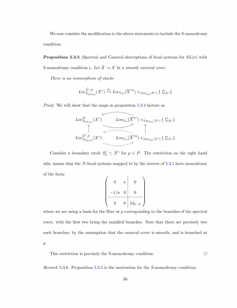
We now consider the modification to the above statements to include the S-monodromy
condition:
Proposition 5.3.5 (Spectral and Cameral descriptions of local systems for SL(n) with
S-monodromy condition.). Let X → X be a smooth cameral cover.
There is an isomorphism of stacks
LocX◦,S
NSL(n)(X◦)
∼=−→ LocGm(X◦R)×LocGm (X◦) { CX◦}
Proof. We will show that the maps in proposition 5.3.4 factors as
LocX◦
NSL(n)(X◦) LocGm(X
◦P )×LocGm (X◦) { CX◦}
LocX◦,S
NSL(n)(X◦) LocGm(X
◦R)×LocGm (X◦) { CX◦}
Consider a boundary circle S1p ⊂ X◦ for p ∈ P . The restriction on the right hand
side, means that the N -local systems mapped to by the inverse of 5.3.1 have monodromy
of the form:
0 a 0
−1/a 0 0
0 0 Idn−2
where we are using a basis for the fiber at p corresponding to the branches of the spectral
cover, with the first two being the ramified branches. Note that there are precisely two
such branches, by the assumption that the cameral cover is smooth, and is branched at
p.
This restriction is precisely the S-monodromy condition.
Remark 5.3.6. Proposition 5.3.5 is the motivation for the S-monodromy condition.
56
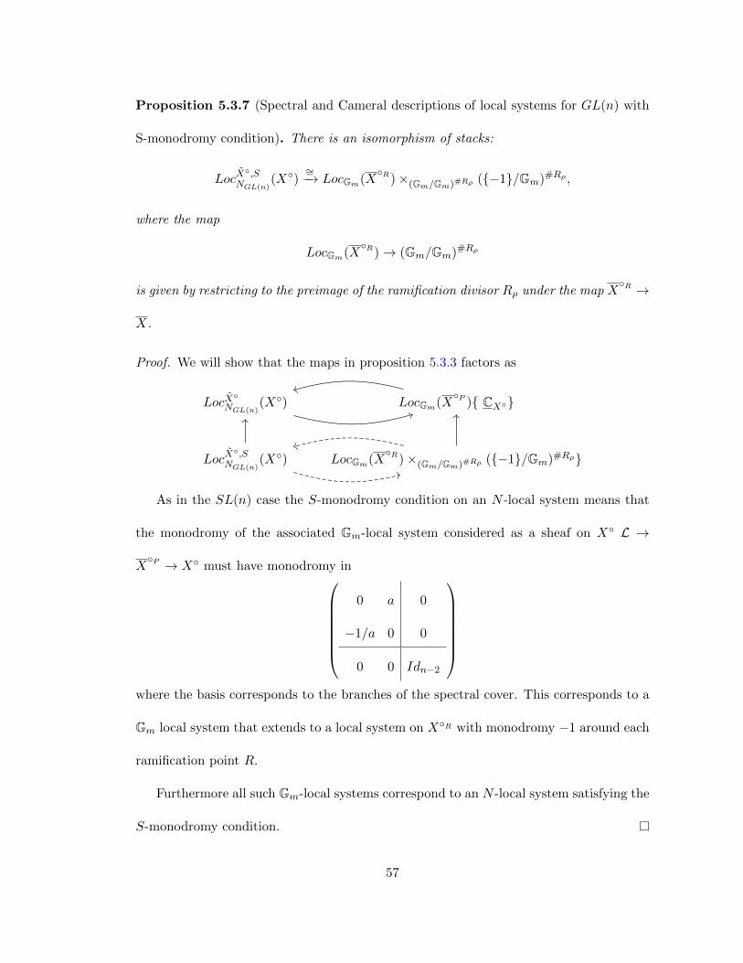
Proposition 5.3.7 (Spectral and Cameral descriptions of local systems for GL(n) with
S-monodromy condition). There is an isomorphism of stacks:
LocX◦,S
NGL(n)(X◦)
∼=−→ LocGm(X◦R)×(Gm/Gm)#Rρ ({−1}/Gm)#Rρ ,
where the map
LocGm(X◦R) → (Gm/Gm)#Rρ
is given by restricting to the preimage of the ramification divisor Rρ under the map X◦R →
X.
Proof. We will show that the maps in proposition 5.3.3 factors as
LocX◦
NGL(n)(X◦) LocGm(X
◦P ){ CX◦}
LocX◦,S
NGL(n)(X◦) LocGm(X
◦R)×(Gm/Gm)#Rρ ({−1}/Gm)#Rρ}
As in the SL(n) case the S-monodromy condition on an N -local system means that
the monodromy of the associated Gm-local system considered as a sheaf on X◦ L →
X◦P → X◦ must have monodromy in
0 a 0
−1/a 0 0
0 0 Idn−2
where the basis corresponds to the branches of the spectral cover. This corresponds to a
Gm local system that extends to a local system on X◦R with monodromy −1 around each
ramification point R.
Furthermore all such Gm-local systems correspond to an N -local system satisfying the
S-monodromy condition.
57
5.3.2 The Case of Sp(2n)
We have that T ∼= Gnm, and W ∼= Sn � {±1}n.
The defining representation Sp(2n)ρ−→ GL(2n) induces a map tSp(2n) → tGL(2n), which
induces a map of the Hitchin bases. By the spectral curve associated to a point in the
Sp(2n) Hitchin base we mean the spectral curve associated to the image of this point
in the GL(2n) Hitchin base. The weights of the defining representation form a single
W -orbit, and we can identify X ∼= Xneρ the non-embedded spectral cover and the spectral
cover in this case.
Proposition 5.3.8 (Non-embedded and embedded spectral covers for Sp(2n), [8]). There
is an isomorphism Xneρ
∼= X.
Proof. Identify t ∼= Cn in a way that intertwines W
�
t with Sn � {±1}n � Cn. Projecting
onto one copy of C gives a map tKXc(D)→ Tot(KXc(D)) that gives rise to the desired
identification.
The involution i : Tot(KXc(D)) → Tot(KXc(D)) coming from the action of−1 preserves
the spectral curve, and hence descends to an involution of X. We also denote the induced
involutions of X◦P and X
◦R by i.
We denote the quotient map by pi: X◦P pi−→ X
◦P /i.
Proposition 5.3.9 (Spectral and Cameral Descriptions for Sp(2n) without S-monodromy
condition. Cf. [20, 8]). There is an isomorphism of stacks
LocX◦
N (X◦)
LocGm
�X
◦P �×LocGm ( X◦P /i) {CX
◦P /i},
∼= (5.3.2)
58
where the map
LocGm(X◦P ) → LocGm(X
◦P /i)
corresponds to the map L �→ det((pi)∗L) (on one dimensional local systems, which are
equivalent to Gm local systems).
Proof. Consider X◦ → X◦P /i as an Stab({α,−α})-bundle, where Stab({α,−α}) ⊂ W is
the stabilizer of the unordered set of the pair of weights {α,−α}.
There is an isomorphism X◦×Stab({α,−α}) (Vα∧V−α) ∼= CX |X◦ because Stab({α,−α}),
acts trivially on Vα ∧ V−α.
Construction 5.1.4 factors through a map as in equation 5.3.2. We will construct an
inverse.
Let L → X◦P be a locally constant line bundle on X
◦P together with a trivialization
of det((pi)∗L).
Let A :=�
−n≤i≤n,i�=0Ci be the disjoint union of 2n copies of C. Consider invertible
homomorphisms from A → A that consist of:
• A permutation σ of {−n, ...,−1, 1, ..., n},
• A linear map Ci → Cσ(i) for each i ∈ {−n, ...,−1, 1, ..., n}.
These can be identified with NGL(2n). We will now describe a subset that can be identified
with NSp(2n) �→ NGL(2n).
For each i ∈ {1, ..., n} define the isomorphism Ci ∧C−i∼=−→ C that sends 1 ∧ 1 to 1 for
i > 0 (and hence 1 ∧ 1 �→ −1 for i < 0).
Define the subset of invertible homomorphisms A → A such that:
59
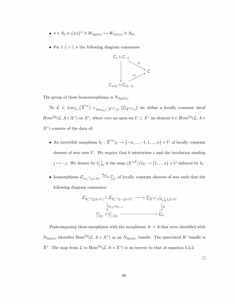
• σ ∈ Sn � {±1}n ∼= WSp(2n) �→ WGL(n)∼= S2n.
• For 1 ≤ i ≤ n the following diagram commutes:
Ci ∧ C−i
C
Cσ(i) ∧ Cσ(−i)
∼=
∼=
The group of these homomorphisms is NSp(2n).
To L ∈ LocGm
�X
◦P � ×LocGm ( X◦P /i) {CX
◦P /i} we define a locally constant sheaf
HomSp(L, A×X◦) on X◦, where over an open set U ⊂ X◦ an element b ∈ HomSp(L, A×
X◦) consists of the data of:
• An invertible morphism b1 : X◦P |U → {−n, ...,−1, 1, ..., n} × U of locally constant
sheaves of sets over U . We require that b intertwines i and the involution sending
j �→ −j. We denote by b−11,K is the map (X◦,P /i)|U → {1, ..., n} × U induced by b1
• Isomorphisms L|w−11 (j×X)
b2,j−−→ Cj , of locally constant sheaves of sets such that the
following diagram commutes:
L|b−11 ({j}×U) ∧ L|b−1
1 ({−j}×U) CX◦P /i|b−1
1,K{j}×U
CjU∧ C−j
UCU
b2,j∧b2,−j ∼=
Postcomposing these morphisms with the morphisms A → A that were identified with
NSp(2n) identifies HomSp(L, A ×X◦) as an NSp(2n) bundle. The associated W bundle is
X◦. The map from L to HomSp(L, A×X◦) is an inverse to that of equation 5.3.2.
60
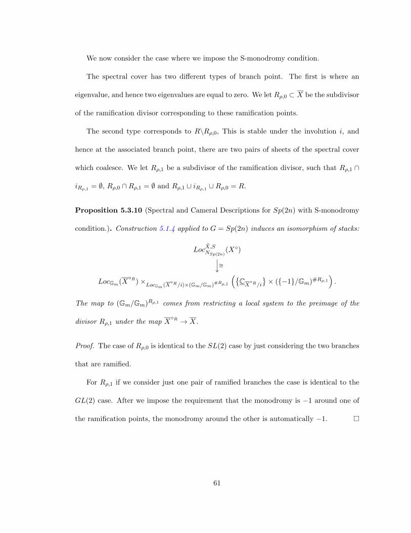
We now consider the case where we impose the S-monodromy condition.
The spectral cover has two different types of branch point. The first is where an
eigenvalue, and hence two eigenvalues are equal to zero. We let Rρ,0 ⊂ X be the subdivisor
of the ramification divisor corresponding to these ramification points.
The second type corresponds to R\Rρ,0, This is stable under the involution i, and
hence at the associated branch point, there are two pairs of sheets of the spectral cover
which coalesce. We let Rρ,1 be a subdivisor of the ramification divisor, such that Rρ,1 ∩
iRρ,1 = ∅, Rρ,0 ∩Rρ,1 = ∅ and Rρ,1 ∪ iRρ,1 ∪Rρ,0 = R.
Proposition 5.3.10 (Spectral and Cameral Descriptions for Sp(2n) with S-monodromy
condition.). Construction 5.1.4 applied to G = Sp(2n) induces an isomorphism of stacks:
LocX,SNSp(2n)
(X◦)
LocGm(X◦R)×
LocGm (X◦R/i)×(Gm/Gm)#Rρ,1
��CX
◦R/i
�× ({−1}/Gm)#Rρ,1
�.
∼=
The map to (Gm/Gm)Rρ,1 comes from restricting a local system to the preimage of the
divisor Rρ,1 under the map X◦R → X.
Proof. The case of Rρ,0 is identical to the SL(2) case by just considering the two branches
that are ramified.
For Rρ,1 if we consider just one pair of ramified branches the case is identical to the
GL(2) case. After we impose the requirement that the monodromy is −1 around one of
the ramification points, the monodromy around the other is automatically −1.
61
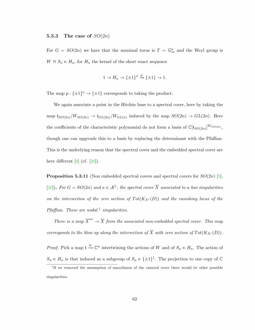
5.3.3 The case of SO(2n)
For G = SO(2n) we have that the maximal torus is T = Gnm and the Weyl group is
W ∼= Sn �Hn, for Hn the kernel of the short exact sequence
1 → Hn → {±1}n p−→ {±1} → 1.
The map p : {±1}n → {±1} corresponds to taking the product.
We again associate a point in the Hitchin base to a spectral cover, here by taking the
map tSO(2n)/WSO(2n) → tGL(2n)/WGL(n) induced by the map SO(2n) → GL(2n). Here
the coefficients of the characteristic polynomial do not form a basis of C[tSO(2n)]WSO(2n) ,
though one can upgrrade this to a basis by replacing the determinant with the Pfaffian.
This is the underlying reason that the spectral cover and the embedded spectral cover are
here different [8] (cf. [20]).
Proposition 5.3.11 (Non embedded spectral covers and spectral covers for SO(2n) [8],
[20]). For G = SO(2n) and a ∈ A♦, the spectral cover X associated to a has singularities
on the intersection of the zero section of Tot(KXc(D)) and the vanishing locus of the
Pfaffian. These are nodal 1 singularities.
There is a map Xne → X from the associated non-embedded spectral cover. This map
corresponds to the blow up along the intersection of X with zero section of Tot(KXc(D)).
Proof. Pick a map t∼=−→ Cn intertwining the actions of W and of Sn �Hn. The action of
Sn �Hn is that induced as a subgroup of Sn � {±1}1. The projection to one copy of C1If we removed the assumption of smoothness of the cameral cover there would be other possible
singularities.
62
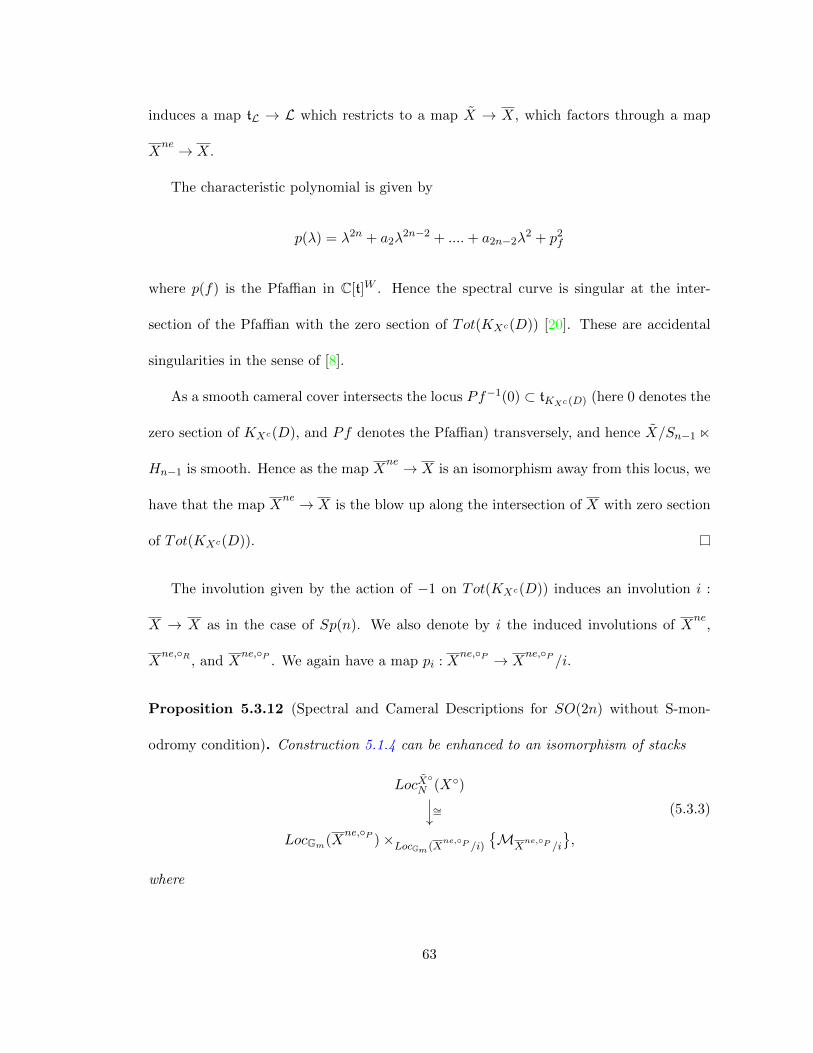
induces a map tL → L which restricts to a map X → X, which factors through a map
Xne → X.
The characteristic polynomial is given by
p(λ) = λ2n + a2λ2n−2 + ....+ a2n−2λ
2 + p2f
where p(f) is the Pfaffian in C[t]W . Hence the spectral curve is singular at the inter-
section of the Pfaffian with the zero section of Tot(KXc(D)) [20]. These are accidental
singularities in the sense of [8].
As a smooth cameral cover intersects the locus Pf−1(0) ⊂ tKXc (D) (here 0 denotes the
zero section of KXc(D), and Pf denotes the Pfaffian) transversely, and hence X/Sn−1 �
Hn−1 is smooth. Hence as the map Xne → X is an isomorphism away from this locus, we
have that the map Xne → X is the blow up along the intersection of X with zero section
of Tot(KXc(D)).
The involution given by the action of −1 on Tot(KXc(D)) induces an involution i :
X → X as in the case of Sp(n). We also denote by i the induced involutions of Xne,
Xne,◦R , and X
ne,◦P . We again have a map pi : Xne,◦P → X
ne,◦P /i.
Proposition 5.3.12 (Spectral and Cameral Descriptions for SO(2n) without S-mon-
odromy condition). Construction 5.1.4 can be enhanced to an isomorphism of stacks
LocX◦
N (X◦)
LocGm(Xne,◦P )×LocGm (X
ne,◦P /i)
�MX
ne,◦P /i
�,
∼= (5.3.3)
where
63
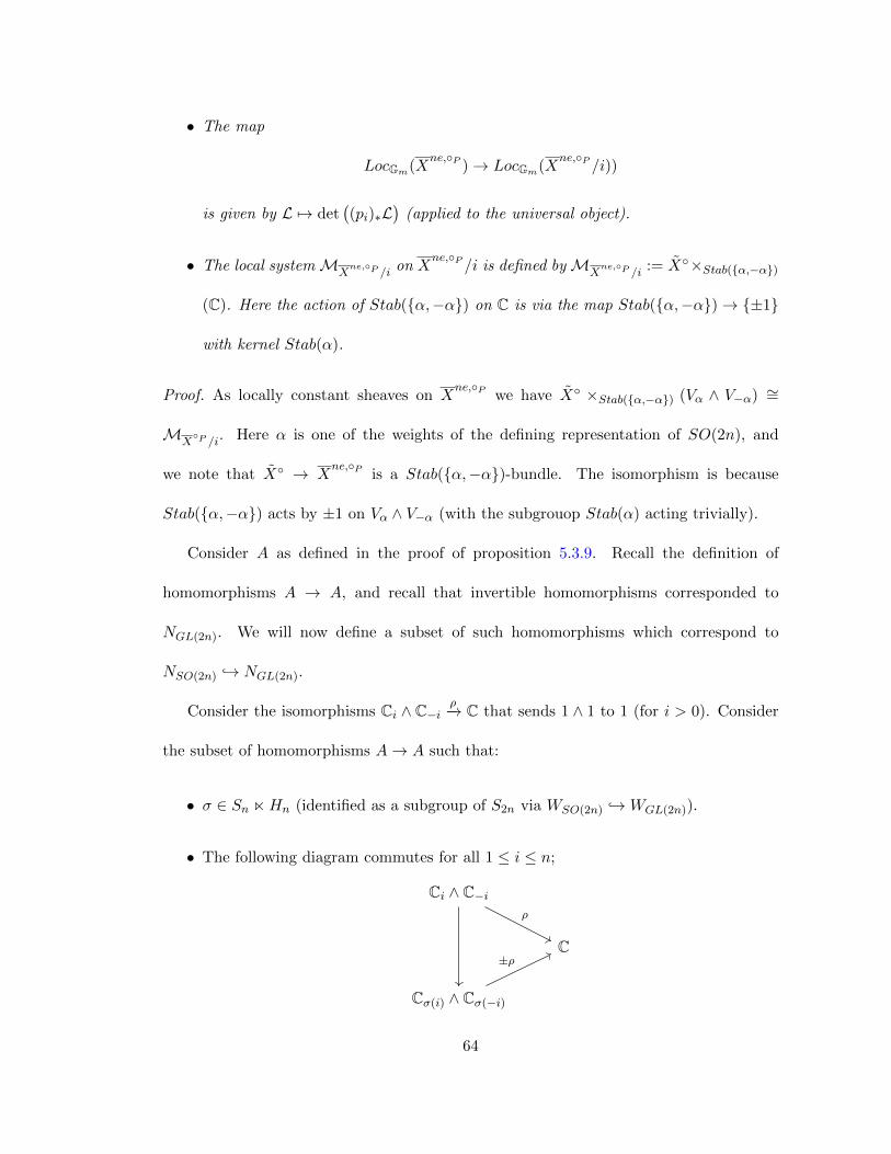
• The map
LocGm(Xne,◦P ) → LocGm(X
ne,◦P /i))
is given by L �→ det�(pi)∗L
�(applied to the universal object).
• The local system MXne,◦P /i on X
ne,◦P /i is defined by MXne,◦P /i := X◦×Stab({α,−α})
(C). Here the action of Stab({α,−α}) on C is via the map Stab({α,−α}) → {±1}
with kernel Stab(α).
Proof. As locally constant sheaves on Xne,◦P we have X◦ ×Stab({α,−α}) (Vα ∧ V−α) ∼=
MX◦P /i. Here α is one of the weights of the defining representation of SO(2n), and
we note that X◦ → Xne,◦P is a Stab({α,−α})-bundle. The isomorphism is because
Stab({α,−α}) acts by ±1 on Vα ∧ V−α (with the subgrouop Stab(α) acting trivially).
Consider A as defined in the proof of proposition 5.3.9. Recall the definition of
homomorphisms A → A, and recall that invertible homomorphisms corresponded to
NGL(2n). We will now define a subset of such homomorphisms which correspond to
NSO(2n) �→ NGL(2n).
Consider the isomorphisms Ci ∧ C−iρ−→ C that sends 1 ∧ 1 to 1 (for i > 0). Consider
the subset of homomorphisms A → A such that:
• σ ∈ Sn �Hn (identified as a subgroup of S2n via WSO(2n) �→ WGL(2n)).
• The following diagram commutes for all 1 ≤ i ≤ n;
Ci ∧ C−i
C
Cσ(i) ∧ Cσ(−i)
ρ
±ρ
64
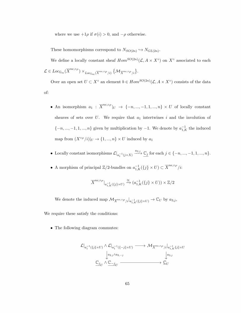
where we use +1ρ if σ(i) > 0, and −ρ otherwise.
These homomorphisms correspond to NSO(2n) �→ NGL(2n).
We define a locally constant sheaf HomSO(2n)(L, A × X◦) on X◦ associated to each
L ∈ LocGm(Xne,◦P )×LocGm (X
ne,◦P /i)
�MX
ne,◦P /i
�.
Over an open set U ⊂ X◦ an element b ∈ HomSO(2n)(L, A×X◦) consists of the data
of:
• An isomorphism a1 : Xne,◦P |U → {−n, ...,−1, 1, ..., n} × U of locally constant
sheaves of sets over U . We require that a1 intertwines i and the involution of
{−n, ...,−1, 1, ..., n} given by multiplication by −1. We denote by a−11,K the induced
map from (X◦P /i)|U → {1, ..., n} × U induced by a1
• Locally constant isomorphisms L|a−11 (j×X)
a2,j−−→ Cj for each j ∈ {−n, ...,−1, 1, ..., n}.
• A morphism of principal Z/2-bundles on a−11,K({j} × U) ⊂ X
ne,◦P /i:
Xne,◦P |a−1
1,K({j}×U)
∼=−→ (a−11,K({j} × U))× Z/2
We denote the induced map MXne,◦P /i|a−1
1,K({j}×U) → CU by a3,j ,
We require these satisfy the conditions:
• The following diagram commutes:
L|a−11 ({j}×U) ∧ L|a−1
1 ({−j}×U) MXne,◦P /i|a−1
1,K{j}×U
CjU∧ C−j
UCU
a2,j∧a2,−j a3,j
65
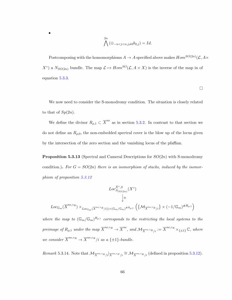
•2n�
(⊕−n<j<n,j �=0b2,j) = Id.
Postcomposing with the homomorphismsA → A specified above makesHomSO(2n)(L, A×
X◦) a NSO(2n) bundle. The map L �→ HomSO(L, A×X) is the inverse of the map in of
equation 5.3.3.
We now need to consider the S-monodromy condition. The situation is closely related
to that of Sp(2n).
We define the divisor Rρ,1 ⊂ Xne
as in section 5.3.2. In contrast to that section we
do not define an Rρ,0, the non-embedded spectral cover is the blow up of the locus given
by the intersection of the zero section and the vanishing locus of the pfaffian.
Proposition 5.3.13 (Spectral and Cameral Descriptions for SO(2n) with S-monodromy
condition.). For G = SO(2n) there is an isomorphism of stacks, induced by the isomor-
phism of proposition 5.3.12
LocX◦,S
NSO(2n)(X◦)
LocGm(Xne,◦R)×
LocGm (Xne,◦R/i))×(Gm/Gm)#Rρ,1
��MX
ne,◦R/i
�× (−1/Gm)#Rρ,1
�∼=
where the map to (Gm/Gm)Rρ,1 corresponds to the restricting the local systems to the
preimage of Rρ,1 under the map Xne,◦R → X
ne, and MX
ne,◦R/i := Xne,◦R ×{±1}C, where
we consider Xne,◦R → X
ne,◦R/i as a {±1}-bundle.
Remark 5.3.14. Note thatMXne,◦R/i|Xne,◦P /i
∼= MXne,◦R/i (defined in proposition 5.3.12).
66
Proof. The analysis is identical to that of Proposition 5.3.10, with the exception of the
fact we do not need to consider Rρ,0 as mentioned above.
67
5.3.4 The case of SO(2n+ 1)
For G = SO(2n + 1), the maximal torus is T ∼= Gnm, and the Weyl group is W ∼=
Sn � {±1}n.
The weights of the defining representations consist of two W -orbits, one consisting of
the single weight 0, and one of all the other weights of this representation
We again associate a spectral cover X to a point in the Hitchin base, by considering
the induced map tSO(2n+1)/WSO(2n+1) → tGL(2n+1)/WGL(2n+1) from the map of groups
SO(2n + 1) → GL(2n + 1). For a ∈ A♦ the associated spectral cover has a partial nor-
malization X0�
X1 → X, where X0 corresponds to the zero weight, and X1 corresponds
to the other W -orbit. Note that this map is an isomorphism when restricted away from
the locus where X1 → Tot(KXc(D)) intersects the zero section, because X0 corresponds
to the zero section of Tot(KXc(D)).
We can identify this disjoint union with the non-embedded spectral cover:
Proposition 5.3.15. There is an isomorphism
X1
�X0
∼= Xneρ .
Proof. We use the decomposition of the non-embedded spectral cover coming from de-
composing Ωρ into W -orbits in equation 5.1.1. Denote the orbits by 0, and 1 and write
Xne,0
and Xne,1
to denote the corresponding subschemes of the non-embedded spectral
cover Xneρ . Then X
ne,0 ∼= X ∼= X0. The identification of Xne,1 ∼= X1 is identical to the
identification in proposition 5.3.8.
As in the case of Sp(2n) and SO(2n) we have an involution i : Xρ → Xρ coming from
the action of −1 on Tot(KXc(D)).
68

This involution fixes X0 pointwise. This involution maps X1 to X1.
We decompose the ramification locus as Rρ = Ra�
Rb where Ra ⊂ X1, and Rb ⊂ X0
be the ramification locus of the map Xneρ → X. We denote by X
◦R1 and X
◦R0 the oriented
real blow ups of X1 and X0 at Ra and Rb respectively. The analysis of the ramification
points is closely related to that of Sp(2n); we have two types of branch points, the first is
where X1 intersects the zero section. We note that by the symmetry of X at such a point
X1 → X is ramified. The second is points in R\(R ∩X0). As in the Sp(2n) these come
in pairs, and so as in the Sp(2n) case we decompose Ra = Rρ,0�
Rρ,1�
i(Rρ,1), where
Rρ,0, Rρ,1, i(Rρ,1) are effective divisors corresponding to disjoint sets of points.
Proposition 5.3.16 (Spectral and Cameral Descriptions for SO(2n + 1) with S-mon-
odromy condition. Cf. [20, 8]). For G = SO(2n + 1) construction 5.1.4 induces an
isomorphism:
LocX◦,S
NSO(2n+1)(X◦)
LocGm(Xne,◦R)×
LocGm (Xne,◦R/i)×(Gm/Gm)#Rρ,1
�{M} × (−1/Gm)#Rρ,1
�,
∼=
where the map
LocGm(Xne,◦R) → LocGm(X
ne,◦R/i)
corresponds to the map L �→ det((pi)∗L), and the map to (Gm/Gm)#Rρ,1 corresponds to
taking the monodromy around each point in Rρ,1.
The Gm-local system M is defined on X◦R0 /i by M|X◦R
0:= X◦×W V0, where V0 is the
representation of W coming from the N -action on the zero weight space of the defining
69
representation of SO(2n+1). On X◦R1 /i it is defined by M|X◦R
1 /i := X◦×Stab({α,−α}) (C),
where Stab({α,−α}) acts on C via the map Stab({α,−α}) → {±1} with kernel Stab(α).
Proof. We first note that the map of 5.1.4 does induce such a map. The argument the
induced line bundle on X◦R1 /i is M|X◦R
1 /i is identical to that in the SO(2n) case of
propositions 5.3.12, 5.3.13.
The local system induced on X◦R0
∼= X◦ is then given by:
X◦ ×W V0,
where V0 is the representation ofW on the zero-weight space of the defining representation
of SO(2n+ 1). Note that this is the representation
Sn � {±1}n → {±1} � C,
where the map corresponds to taking the product of the ±1 factors, and the action on C
is by multiplication.
Consider A as defined in the proof of proposition 5.3.9. Recall the definition of ho-
momorphisms A → A. We will define a subset of the invertible homomorphisms that we
identify with NSO(2n+1.
Consider the isomorphisms Ci ∧C−iρ−→ C sending 1∧ 1 to 1 (for i > 0) that were also
defined previously.
Consider the subset of invertible homommorphisms A → A such that.
• σ ∈ Sn � {±1}n (identified as a subgroup of S2n via the map WSO(2n+1) �→
WGL(2n+1) factoring through WGL(2n)).
70
• The following diagram commutes for all 1 ≤ i ≤ n;
Ci ∧ C−i
C
Cσ(i) ∧ Cσ(−i)
ρ
±ρ
where we use +1ρ if σ(i) > 0, and −ρ otherwise.
We can identify the homomorphisms satisfying these conditions with NSO(2n+1).
Consider the locally constant sheaf on X◦ associated to
L ∈ LocGm(X◦P1 )×LocGm (X
ne,◦P /i) {M}
denoted by HomSO(2n+1)(L|Xne,◦P1
, A×X◦), where over an open set U ⊂ X◦ an element
a ∈ HomSO(2n)(L, C ×X◦) consists of the data of;
• An isomorphism a1 : Xne,◦P |U → {−n, ...,−1, 1, ..., n} × U of locally constant
sheaves of sets over U . We require that a1 intertwines i and the involution of
{−n, ...,−1, 1, ..., n} given by multiplication by −1. We denote by a−11,K the induced
map from (X◦P /i)|U → {1, ..., n} × U induced by a1
• Locally constant isomorphisms L|a−11 (j×X)
a2,j−−→ Cj for each j ∈ {−n, ...,−1, 1, ..., n}.
• Morphisms of principal Z/2-bundles on b−11,K({j}×U) ⊂ X
◦P /i fromX◦P |b−1
1,K({j}×U)
∼=−→
(b−11,K({j} × U)) × Z/2. We denote by a3,j : MX
◦P /i|b−11,K({j}×U) → CU the induced
map of locally constant sheaves of vector bundles.
We require that;
71
• The following diagram commutes:
L|a−11 ({j}×U) ∧ L|a−1
1 ({−j}×U) MX◦P /i|a−1
1,K{j}×U
CjU∧ C−j
UCU
a2,j∧a2,−j a3,j
Postcomposing withA → A corresponding to n ∈ NSO(2n+1) givesHomSO(2n+1)(L|Xne,◦R1
, A×
X◦) the structure of a NSO(2n+1) bundle. The map L �→ HomSO(2n+1)(L, A×X) is then
the inverse to the map in proposition 5.3.16.
We now consider the S-monodromy. Considering the effect on the monodromy around
Rρ,1 is analogous to the SO(2n) and Sp(2n) cases in the proof of propositions 5.3.10 and
5.3.13. The effect at Rρ,0 is analogous to that of Sp(2n) in proposition 5.3.10, As the
monodromy of the local system on X0 then restricts the monodromy to be −1, we have
to restrict the monodromy of the system on X1 around r ∈ Rρ,0 to be −1. The result
follows.
72
Bibliography
[1] Takashi Aoki, Naofumi Honda, Takahiro Kawai, Tatsuya Koike, Yukihiro Nishikawa,
Shunsuke Sasaki, Akira Shudo, and Yoshitsugu Takei, Virtual turning points—a gift
of microlocal analysis to the exact WKB analysis, Algebraic Analysis of Differential
Equations, Springer, 2008, pp. 29–43.
[2] Takashi Aoki, Takahiro Kawai, Shunsuke Sasaki, Akira Shudo, and Yoshitsugu Takei,
Virtual turning points and bifurcation of Stokes curves for higher order ordinary
differential equations, Journal of Physics A: Mathematical and General 38 (2005),
no. 15, 3317.
[3] Takashi Aoki, Takahiro Kawai, and Yoshitsugu Takei, On the exact steepest descent
method: a new method for the description of Stokes curves, Journal of Mathematical
Physics 42 (2001), no. 8, 3691–3713.
[4] Arnaud Beauville, MS a Narasimhan, and S Ramanan, Spectral curves and the gen-
eralised theta divisor, J. reine angew. Math 398 (1989), 169–179.
[5] H. L. Berk, William McCay Nevins, and K. V. Roberts, New Stokes’ line in WKB
theory, Journal of Mathematical Physics 23 (1982), no. 6, 988–1002.
73
[6] Tom Bridgeland and Ivan Smith, Quadratic differentials as stability conditions, Pub-
lications mathematiques de l’IHES 121 (2015), no. 1, 155–278.
[7] C. Chevalley, Sur certains groupes simples, Tohoku Math. J. (2) 7 (1955), no. 1-2,
14–66.
[8] Ron Donagi, Decomposition of spectral covers, Asterisque 218 (1993), 145–175.
[9] Ron Donagi and Dennis Gaitsgory, The gerbe of Higgs bundles, Transformation
groups 7 (2002), no. 2, 109–153.
[10] Gerd Faltings, Stable G-bundles and projective connections, J. Algebraic Geom 2
(1993), no. 3, 507–568.
[11] Aaron Fenyes, A dynamical perspective on shear-bend coordinates, arXiv preprint
arXiv:1510.05757 (2015).
[12] Vladimir Fock and Alexander Goncharov, Moduli spaces of local systems and higher
Teichmuller theory, Publications Mathematiques de l’Institut des Hautes Etudes
Scientifiques 103 (2006), no. 1, 1–211.
[13] Davide Gaiotto, Gregory W Moore, and Andrew Neitzke, Four-dimensional wall-
crossing via three-dimensional field theory, Communications in Mathematical Physics
299 (2010), no. 1, 163–224.
[14] , Wall-crossing in coupled 2d-4d systems, Journal of High Energy Physics
2012 (2012), no. 12, 82.
74
[15] , Framed BPS states, Advances in Theoretical and Mathematical Physics 17
(2013), no. 2, 241–397.
[16] , Spectral networks, Annales Henri Poincare, vol. 14, Springer, 2013, pp. 1643–
1731.
[17] , Wall-crossing, Hitchin systems, and the WKB approximation, Advances in
Mathematics 234 (2013), 239–403.
[18] , Spectral networks and snakes, Annales Henri Poincare, vol. 15, Springer,
2014, pp. 61–141.
[19] Richard M Green, Combinatorics of minuscule representations, vol. 199, Cambridge
University Press, 2013.
[20] Nigel J. Hitchin, Stable bundles and integrable systems, Duke mathematical journal
54 (1987), no. 1, 91–114.
[21] Lotte Hollands and Andrew Neitzke, Spectral networks and Fenchel–Nielsen coordi-
nates, Letters in Mathematical Physics 106 (2016), no. 6, 811–877.
[22] Naofumi Honda, Takahiro Kawai, and Yoshitsugu Takei, Virtual turning points,
Springer, 2015.
[23] Matei Ionita and Benedict Morrissey, Spectral Networks and Non-abelianization,
Preprint, 14th April, 2020.
[24] Kohei Iwaki and Tomoki Nakanishi, Exact WKB analysis and cluster algebras, Jour-
nal of Physics A: Mathematical and Theoretical 47 (2014), no. 47, 474009.
75
[25] , Exact WKB analysis and cluster algebras II: Simple poles, orbifold points,
and generalized cluster algebras, International Mathematics Research Notices 2016
(2015), no. 14, 4375–4417.
[26] Pietro Longhi, Andrew Neitzke, and Chan Y Park, Loom, https://github.com/
chan-y-park/loom.
[27] Pietro Longhi and Chan Y Park, ADE spectral networks, Journal of High Energy
Physics 2016 (2016), no. 8, 87.
[28] Jacob Lurie, Spectral algebraic geometry.
[29] , Higher topos theory, Princeton University Press, 2009.
[30] Bao Chau Ngo, Le lemme fondamental pour les algebres de Lie, Publications
mathematiques de l’IHES 111 (2010), no. 1, 1–169.
[31] Daniel Schaub, Courbes spectrales et compactifications de jacobiennes, Mathematis-
che Zeitschrift 227 (1998), no. 2, 295–312.
[32] Renata Scognamillo, An elememtary approach to the abelianization of the Hitchin
system for arbitrary reductive groups, Compositio Mathematica 110 (1998), no. 1,
17–37.
[33] Kurt Strebel, Quadratic differentials, vol. 5, Springer Science & Business Media,
1984.
76
[34] Yoshitsugu Takei, WKB analysis and Stokes geometry of differential equations, An-
alytic, algebraic and geometric aspects of differential equations, Springer, 2017,
pp. 263–304.
[35] William P Thurston, Minimal stretch maps between hyperbolic surfaces, arXiv
preprint math/9801039 (1998).
[36] Bertrand Toen and Gabriele Vezzosi, From HAG to DAG: derived moduli stacks,
Axiomatic, enriched and motivic homotopy theory, Springer, 2004, pp. 173–216.
[37] , Homotopical Algebraic Geometry II: Geometric Stacks and Applications,
vol. 2, American Mathematical Soc., 2008.
77