A Discriminative Model for Semi-Supervised Learningninamf/papers/ssl-2009.pdf · A Discriminative Model for Semi-Supervised Learning ∗ Maria-Florina Balcan School of Computer Science,

A Discriminative Model for Semi-Supervised

Learning ∗

Maria-Florina Balcan

School of Computer Science, Georgia Institute of Technology

Avrim Blum

Computer Science Department, Carnegie Mellon University

Supervised learning — that is, learning from labeled examples — is an area of Machine Learningthat has reached substantial maturity. It has generated general-purpose and practically-successfulalgorithms and the foundations are quite well understood and captured by theoretical frameworkssuch as the PAC-learning model and the Statistical Learning theory framework. However, for manycontemporary practical problems such as classifying web pages or detecting spam, there is oftenadditional information available in the form of unlabeled data, which is often much cheaper andmore plentiful than labeled data. As a consequence, there has recently been substantial interestin semi-supervised learning — using unlabeled data together with labeled data — since any usefulinformation that reduces the amount of labeled data needed can be a significant benefit. Severaltechniques have been developed for doing this, along with experimental results on a variety ofdifferent learning problems. Unfortunately, the standard learning frameworks for reasoning aboutsupervised learning do not capture the key aspects and the assumptions underlying these semi-supervised learning methods.

In this paper we describe an augmented version of the PAC model designed for semi-supervised

learning, that can be used to reason about many of the different approaches taken over the pastdecade in the Machine Learning community. This model provides a unified framework for ana-lyzing when and why unlabeled data can help, in which one can analyze both sample-complexityand algorithmic issues. The model can be viewed as an extension of the standard PAC modelwhere, in addition to a concept class C, one also proposes a compatibility notion: a type of com-patibility that one believes the target concept should have with the underlying distribution ofdata. Unlabeled data is then potentially helpful in this setting because it allows one to estimatecompatibility over the space of hypotheses, and to reduce the size of the search space from thewhole set of hypotheses C down to those that, according to one’s assumptions, are a-priori reason-able with respect to the distribution. As we show, many of the assumptions underlying existingsemi-supervised learning algorithms can be formulated in this framework.

After proposing the model, we then analyze sample-complexity issues in this setting: that is,how much of each type of data one should expect to need in order to learn well, and what the keyquantities are that these numbers depend on. We also consider the algorithmic question of how toefficiently optimize for natural classes and compatibility notions, and provide several algorithmicresults including an improved bound for Co-Training with linear separators when the distributionsatisfies independence given the label.

∗ A preliminary version of this paper appears as “A PAC-style Model for Learning from Labeledand Unlabeled Data”, Proc. 18th Annual Conference on Learning Theory (COLT), pp. 111−1264,

2005, and portions appear as Chapter 22 of the book Semi-Supervised Learning [Chapelle et al.2006]. This work was supported in part by NSF grants IIS-0312814 and CCR-0105488 and byan IBM Graduate Fellowship. This work was done in part while the first author was at CarnegieMellon University.Permission to make digital/hard copy of all or part of this material without fee for personalor classroom use provided that the copies are not made or distributed for profit or commercialadvantage, the ACM copyright/server notice, the title of the publication, and its date appear, andnotice is given that copying is by permission of the ACM, Inc. To copy otherwise, to republish,to post on servers, or to redistribute to lists requires prior specific permission and/or a fee.c© 20YY ACM 0000-0000/20YY/0000-0001 $5.00

ACM Journal Name, Vol. V, No. N, Month 20YY, Pages 1–0??.

Categories and Subject Descriptors: I.5.1 [ Pattern Recognition]: Models; F.2.0 [Analysis

of Algorithms and Problem Complexity]: General; G.3 [Probability and Statistics]:Correlation and regression analysis

General Terms: Algorithms, Theory.

Additional Key Words and Phrases: Machine Learning, Semi-Supervised Learning, Value of Un-labeled Data, Sample Complexity, Cover Bounds, Uniform Convergence Bounds, Structural RiskMinimization (SRM), Data Dependent SRM, Efficient Learning Algorithms, Multi-view Classifi-cation, Co-training.

1. INTRODUCTION

In recent years there has been substantial and growing interest in using unlabeleddata together with labeled data in machine learning. The motivation is clear: inmany applications, unlabeled data can be much cheaper and much more plentifulthan labeled data. If useful information can be extracted from unlabeled exam-ples that allows for learning from fewer labeled examples, this can be a substantialbenefit. A number of Semi-Supervised learning techniques have been developed fordoing this, along with experimental results on a variety of different learning prob-lems. These include label propagation for word-sense disambiguation [Yarowsky1995], co-training for classifying web pages [Blum and Mitchell 1998] and improv-ing visual detectors [Levin et al. 2003], transductive SVM [Joachims 1999] andEM [Nigam et al. 2000] for text classification, graph-based methods [Zhu et al.2003c], and others. The problem of learning from labeled and unlabeled data hasbeen the topic of several ICML workshops [Ghani et al. 2003; Amini et al. 2005] aswell as a recent book [Chapelle et al. 2006] and survey article [Zhu 2006].

What makes unlabeled data so useful and what many of these methods exploit, isthat for a wide variety of learning problems, the natural regularities of the probleminvolve not only the form of the function being learned by also how this functionrelates to the distribution of data. For example, in many problems one might expectthe target function should cut through low density regions of the space, a propertyused by the transductive SVM algorithm [Joachims 1999]. In other problems onemight expect the target to be self-consistent in some way, a property used by Co-training [Blum and Mitchell 1998]. Unlabeled data is potentially useful in thesesettings because it then allows one to reduce the search space to a set which isa-priori reasonable with respect to the underlying distribution.

Unfortunately, however, the underlying assumptions of these semi-supervisedlearning methods are not captured well by standard theoretical models. The maingoal of this work is to propose a unified theoretical framework for semi-supervisedlearning, in which one can analyze when and why unlabeled data can help, and inwhich one can discuss both sample-complexity and algorithmic issues in a discrim-inative (PAC-model style) framework.

One difficulty from a theoretical point of view is that standard discriminativelearning models do not allow one to specify relations that one believes the tar-get should have with the underlying distribution. In particular, both in the PACmodel [Valiant 1984; Blumer et al. 1989; Kearns and Vazirani 1994] and the Sta-tistical Learning Theory framework [Vapnik 1998] there is intentionally a complete

2

· 3

disconnect between the data distribution D and the target function f being learned.The only prior belief is that f belongs to some class C: even if the data distributionD is known fully, any function f ∈ C is still possible. For instance, in the PACmodel, it is perfectly natural (and common) to talk about the problem of learning aconcept class such as DNF formulas [Linial et al. 1989; Verbeurgt 1990] or an inter-section of halfspaces [Baum 1990; Blum and Kannan 1997; Vempala 1997; Klivanset al. 2002] over the uniform distribution; but clearly in this case unlabeled data isuseless — you can just generate it yourself. For learning over an unknown distribu-tion, unlabeled data can help somewhat in the standard models (e.g., by allowingone to use distribution-specific algorithms and sample-complexity bounds [Benedekand Itai 1991; Kaariainen 2005]), but this does not seem to capture the power ofunlabeled data in practical semi-supervised learning methods. In fact, a recentresult of Simon [2009] shows that the information-theoretic advantage provided byknowing the distribution in the standard PAC model is extremely limited.

In generative models, one can easily talk theoretically about the use of unlabeleddata, e.g., [Castelli and Cover 1995; 1996]. However, these results typically makestrong assumptions that essentially imply that there is only one natural distinc-tion to be made for a given (unlabeled) data distribution. For instance, a typicalgenerative model would be that we assume positive examples are generated by oneGaussian, and negative examples are generated by another Gaussian. In this case,given enough unlabeled data, we could in principle recover the Gaussians and wouldneed labeled data only to tell us which Gaussian is the positive one and which isthe negative one.1 However, this is too strong an assumption for most real-worldsettings. Instead, we would like our model to allow for a distribution over data (e.g.,documents we want to classify) where there are a number of plausible distinctionswe might want to make. In addition, we would like a general framework that canbe used to model many different uses of unlabeled data.

1.1 Overview of Our Model

In this paper, we present a PAC-style framework that bridges between these posi-tions and can be used to help think about and analyze many of the ways unlabeleddata is typically used. This framework extends the PAC learning model in a waythat allows one to express not only the form of target function one is considering,but also relationships that one hopes the target function and underlying distribu-tion will possess. We then analyze both sample-complexity issues—that is, howmuch of each type of data one should expect to need in order to learn well—aswell as algorithmic results in this model. We derive bounds for both the realizable(PAC) and agnostic (statistical learning framework) settings.

We focus for most of this paper on inductive binary classification. In this setting,we assume that our data comes according to a fixed unknown distribution D over aninstance space X , and is labeled by some unknown target function c∗ : X → 0, 1.As in the standard PAC model, in the “realizable case”, we make the assumptionthat the target is in a given class concept class C, whereas in the “agnostic case”we do not make this assumption and instead aim to compete with the best function

1[Castelli and Cover 1995; 1996] do not assume Gaussians in particular, but they do assume thedistributions are distinguishable, which from this perspective has the same issue.

ACM Journal Name, Vol. V, No. N, Month 20YY.

4 ·in the given class C. A learning algorithm is given a set of labeled examples drawni.i.d. from D and labeled by c∗ as well as a (usually larger) set of unlabeled examplesfrom D. The goal is to perform some optimization over these samples and to outputa hypothesis that agrees with the target or with the best approximation of the targetin C over most of the distribution.

We now describe how we extend the PAC model to capture the kinds of beliefsand assumptions used in semi-supervised learning. The main idea is to augment thePAC notion of a concept class, which is a set of functions (such as linear separatorsor decision trees), with a notion of compatibility between a function and the datadistribution that we hope the target function will satisfy. Rather than talking of“learning a concept class C,” we will talk of “learning a concept class C undercompatibility notion χ.” For example, suppose we believe there should exist a low-error linear separator, and that furthermore, if the data happens to cluster, thenthis separator does not slice through the middle of any such clusters. Then wewould want a compatibility notion that penalizes functions that do, in fact, slicethrough clusters. In this framework, the ability of unlabeled data to help dependson two quantities: first, the extent to which the target function indeed satisfiesthe given assumptions, and second, the extent to which the distribution allows thisassumption to rule out alternative hypotheses. For instance, if the data does notcluster at all (say the underlying distribution is uniform in a ball), then all functionswould equally satisfy this compatibility notion and the assumption is not useful.From a Bayesian perspective, one can think of this as a PAC model for a settingin which one’s prior is not just over functions, but also over how the function andunderlying distribution relate to each other.

To make our model formal, we will need to ensure that the degree of compatibilitybe something that can be estimated from a finite sample. To do this, we will requirethat the compatibility notion χ in fact be a function from C ×X to [0, 1], where thecompatibility of a hypothesis h with the data distribution D is then Ex∼D[χ(h, x)].That is, we require that the degree of incompatibility be a kind of unlabeled lossfunction, and the incompatibility of a hypothesis h with a data distribution D is aquantity we can think of as an “unlabeled error rate” that measures how a-prioriunreasonable we believe some proposed hypothesis to be. For instance, in theexample above of a “margin-style” compatibility, we could define χ(f, x) to be anincreasing function of the distance of x to the separator f . In this case, the unlabelederror rate, 1 − χ(f, D), is a measure of the probability mass close to the proposedseparator. In co-training, where each example x has two “views” (x = 〈x1, x2〉),the underlying belief is that the true target c∗ can be decomposed into functions〈c∗1, c∗2〉 over each view such that for most examples, c∗1(x1) = c∗2(x2). In this case,we can define χ(〈f1, f2〉, 〈x1, x2〉) = 1 if f1(x1) = f2(x2), and 0 if f1(x1) 6= f2(x2).Then the compatibility of a hypothesis 〈f1, f2〉 with an underlying distribution Dis Pr〈x1,x2〉∼D[f1(x1) = f2(x2)].

This framework allows us to analyze the ability of a finite unlabeled sample toreduce our dependence on labeled examples, as a function of (a) the compatibilityof the target function (i.e., how correct we were in our assumption) and (b) variousmeasures of the “helpfulness” of the distribution. In particular, in our model, wefind that unlabeled data can help in several distinct ways.


· 5

(1) If the target function is highly compatible with D and belongs to C, then if wehave enough unlabeled data to estimate compatibility over all f ∈ C, we can inprinciple reduce the size of the search space from C down to just those f ∈ Cwhose estimated compatibility is high. For instance, if D is “helpful”, then theset of such functions will be much smaller than the entire set C and we thusneed many fewer labeled examples to learn well. In the agnostic case, or evenin realizable case if the number of labeled examples is severely limited, we cando (unlabeled)-data-dependent structural risk minimization to trade off labelederror and incompatibility.

(2) By providing an estimate of D, unlabeled data can allow us to use a morerefined distribution-specific notion of “hypothesis space size” such as AnnealedVC-entropy [Devroye et al. 1996], Rademacher complexities [Koltchinskii 2001;Bartlett and Mendelson 2002; Boucheron et al. 2005] or the size of the smallestǫ-cover [Benedek and Itai 1991], rather than VC-dimension [Blumer et al. 1989;Kearns and Vazirani 1994]. In fact, for many natural notions of compatibilitywe find that the sense in which unlabeled data reduces the “size” of the searchspace is best described in these distribution-specific measures.

(3) Finally, if the distribution is especially helpful, we may find that not only doesthe set of compatible f ∈ C have a small ǫ-cover, but also the elements ofthe cover are far apart. In that case, if we assume the target function is fullycompatible, we may be able to learn from even fewer labeled examples than theΩ(1/ǫ) needed just to verify a good hypothesis. For instance, as one applicationof this, we show that under the assumption of independence given the label, onecan efficiently perform Co-Training of linear separators from a single labeledexample!

A key feature of our framework is that it allows us to address the issue of howmuch unlabeled data we should expect to need. Roughly, the “VCdim/ǫ2” formof standard sample complexity bounds now becomes a bound on the number ofunlabeled examples we need to uniformly estimate compatibilities. However, tech-nically, the set whose VC-dimension we now care about is not C but rather a setdefined by both C and χ: that is, the overall complexity depends both on the com-plexity of C and the complexity of the notion of compatibility (see Section 3.1.2).One consequence of our model is that if the target function and data distributionare both well behaved with respect to the compatibility notion, then the sample-size bounds we get for labeled data can substantially beat what one could hope toachieve through pure labeled-data bounds, and we illustrate this with a number ofexamples through the paper.

We can also talk about a transductive analog of our inductive model where oneis given a fixed set S of examples, of which some small random subset is labeled,and the goal is to predict well over S. In this case we again express the relationshipwe hope the target function has with the data through a compatibility notion χ.However, since in this case the compatibility of a given hypothesis is completelydetermined by S (which is known), we will not need to require that compatibilitybe an expectation over unlabeled examples. In this case unlabeled data can helpin the ways (1) and (3) described above.


6 ·1.2 Summary of Main Results

The primary contributions of this paper are three-fold.

(1) As described above, we develop a new discriminative (PAC-style) model forsemi-supervised learning, that can be used to analyze when unlabeled data canhelp and how much unlabeled data is needed in order to gain its benefits, aswell as the algorithmic problems involved.

(2) We present a number of fundamental sample complexity bounds illustratingimportant and subtle issues in this framework. We present both uniform-convergence results—which apply to any algorithm that is able to find rulesof low error and high compatibility—as well as ǫ-cover-based bounds that ap-ply to a more restricted class of algorithms but can be substantially tighter.Our main uniform convergence result (Theorem 11) applies to the fully-agnosticsetting and shows how an algorithm that minimizes the sum of empirical errorplus a regularization term that is a function of the compatibility structure, willachieve a near-optimal tradeoff and strong generalization guarantees. Our mainǫ-cover bound (Theorem 13) then gives even tighter guarantees for algorithmsthat first use the unlabeled data to select a small subclass of hypotheses andthen optimize over them. We also describe several natural, interesting caseswhere the set of highly compatible hypotheses is large but it has a small ep-silon cover; in these cases, the ǫ-cover-based bounds can apply even though withhigh probability there still exist high-error hypotheses in the class consistentwith the labeled and unlabeled examples.

(3) We present several algorithmic results in this model matching the various sam-ple complexity bounds we provide. As a warmup we first present a simplealgorithm for learning disjunctions in the fully realizable case for a simple com-patibility notion (Theorem 17). Next, more interestingly we show how we canefficiently perform a near-optimal data dependent structural risk minimizationin a natural transductive graph-based learning setting (Theorem 18). Finally,we present a new algorithm for Co-Training with linear separators (Theorems20 and 21) that, if the distribution satisfies independence given the label as-sumption, requires only a single labeled example to learn to any desired errorrate ǫ and is computationally efficient (i.e., achieves PAC guarantees). Thissubstantially improves on the results of [Blum and Mitchell 1998] which re-quired enough labeled examples to produce an initial weak hypothesis, and inthe process we get also a simplification to the noisy halfspace learning algorithmof [Blum et al. 1998].

Our framework has helped analyze many existing semi-supervised learning methodsused in practice and has guided the development of new semi-supervised learningalgorithms and analyses. We discuss this further in Section 6.1.

1.3 Structure of this Paper

We begin by describing the general setting in which our results apply as well asseveral examples to illustrate our framework in Section 2. We then give resultsboth for sample complexity (in principle, how much data is needed to learn) andefficient algorithms. In terms of sample-complexity, we start by discussing uniform


· 7

convergence results in Section 3.1. For clarity we begin with the case of finitehypothesis spaces in Section 3.1.1, and then discuss infinite hypothesis spaces inSection 3.1.2. We present results for the agnostic case, where one must trade offlabeled error and incompatibility, in Section 3.1.3. In Section 3.2 we give resultsbased on the notion of ǫ-cover size, which can be substantially tighter though theyrequire algorithms of a specific type (that first use the unlabeled data to choose asmall set of “representative” hypotheses and then choose among the representativesbased on the labeled data).

In Section 4, we give our algorithmic results. Our main results here are an efficientalgorithm for graph-based structural risk minimization, nearly matching the samplecomplexity bounds in Section 3.1.3, and an efficient algorithm for Co-Training withlinear separators, nearly matching the bounds of Section 3.2. In Section 5 we discusstransductive learning, connections with generative models and with other ways ofusing unlabeled data in machine learning, as well as the relationship between ourmodel and the Luckiness Framework [Shawe-Taylor et al. 1998] developed in thecontext of supervised learning. Finally, in Section 6 we discuss some implicationsof our model and present our conclusions, as well a number of open problems.

2. A FORMAL FRAMEWORK

In this section we introduce general notation and terminology we use throughoutthe paper, and describe our model for semi-supervised learning. In particular, weformally define what we mean by a notion of compatibility and we illustrate itthrough a number of examples including margins and co-training.

We will focus on binary classification problems. We assume that our data comesaccording to a fixed unknown distribution D over an instance space X , and islabeled by some unknown target function c∗ : X → 0, 1. A learning algorithm isgiven a set SL of labeled examples drawn i.i.d. from D and labeled by c∗ as wellas a (usually larger) set SU of unlabeled examples from D. The goal is to performsome optimization over the samples SL and SU and to output a hypothesis thatagrees with the target over most of the distribution. In particular, the error rate(also called “0 − 1 loss”) of a given hypothesis f is defined as

err(f) = errD(f) = Prx∼D[f(x) 6= c∗(x)].

For any two hypotheses f1, f2, the distance with respect to D between f1 and f2 isdefined as

d(f1, f2) = dD(f1, f2) = Prx∼D[f1(x) 6= f2(x)].

We will use err(f) to denote the empirical error rate of f on a given labeled sample

(i.e., the fraction of mistakes on the sample) and d(f1, f2) to denote the empiricaldistance between f1 and f2 on a given unlabeled sample (the fraction of the sam-ple on which they disagree). As in the standard PAC model, a concept class orhypothesis space is a set of functions over the instance space X . In the “realizablecase”, we make the assumption that the target is in a given class C, whereas in the“agnostic case” we do not make this assumption and instead aim to compete withthe best function in the given class C.

We now formally describe what we mean by a notion of compatibility. A notionof compatibility is a mapping from a hypothesis f and a distribution D to [0, 1]


8 ·indicating how “compatible” f is with D. In order for this to be estimable froma finite sample, we require that compatibility be an expectation over individualexamples.2 Specifically, we define:

Definition 1. A legal notion of compatibility is a function χ : C × X → [0, 1]where we (overloading notation) define χ(f, D) = Ex∼D[χ(f, x)]. Given a sampleS, we define χ(f, S) to be the empirical average of χ over the sample.

Note: One could also allow compatibility functions over k-tuples of examples, inwhich case our (unlabeled) sample-complexity bounds would simply increase by afactor of k.3

Definition 2. Given compatibility notion χ, the incompatibility of f with D is1 − χ(f, D). We will also call this its unlabeled error rate, errunl(f), when χ andD are clear from context. For a given sample S, we use errunl(f) = 1 − χ(f, S) todenote the empirical average over S.

Finally, we need a notation for the set of functions whose incompatibility is atmost some given value τ .

Definition 3. Given value τ , we define CD,χ(τ) = f ∈ C : errunl(f) ≤ τ.So, e.g., CD,χ(1) = C. Similarly, for a sample S, we define CS,χ(τ) = f ∈ C :errunl(f) ≤ τ.

The transductive case: In transductive learning, one is given a fixed set S ofexamples, of which some small random subset is labeled, and the goal is to predictwell over S. That is, we know which examples we will be tested on up front, andso we can view this as a case of learning from a known distribution (the uniformdistribution over S). Since in this case the compatibility of a given hypothesis iscompletely determined by S (which is known), we will not need to require thatcompatibility be an expectation over unlabeled examples. For this setting or forthe setting in which D is actually known in advance, we can drop this requiremententirely and allow any notion of compatibility χ(f, D) to be legal.

For convenience, we summarize the notation used throughout the paper in Ap-pendix A. We now give several examples to illustrate this framework:

Example 1. Suppose examples are points in Rd and C is the class of linear sep-arators. A natural belief in this setting is that data should be “well-separated”:not only should the target function separate the positive and negative examples,but it should do so by some reasonable margin γ. This is the assumption used byTransductive SVM, also called Semi-Supervised SVM (S3VM) [Joachims 1999; Bie

2One could imagine more general notions of compatibility with the property that they can beestimated from a finite sample and all our results would go through in that case as well. Weconsider the special case where the compatibility is an expectation over individual examples forsimplicity of notation, and because most existing semi-supervised learning algorithms used inpractice do satisfy it.3In other words, in this case χ(f, D) = E(x1,...,xk)∼Dk [χ(f, (x1, ..., xk))]. In order to estimatethis quantity, we simply draw a sample of size n from D, and partition it into n/k groups of size k,namely (xi

1, ..., xik) for i = 1, . . . , n/k; our estimate is then simply the average over those groups,

i.e.,Pn/k

i=1 χ(f, (xi1, ..., xi

k)).


· 9

and Cristianini 2003; Chapelle and Zien 2005]. In this case, if we are given γ upfront, we could define χ(f, x) = 1 if x is farther than distance γ from the hyperplanedefined by f , and χ(f, x) = 0 otherwise. So, the incompatibility of f with D isthe probability mass within distance γ of the hyperplane f · x = 0. Alternatively,if we do not want to commit to a specific γ in advance, we could define χ(f, x) tobe a smooth function of the distance of x to the separator, as done in [Chapelleand Zien 2005]. Note that in contrast, defining compatibility of a hypothesis basedon the largest γ such that D has probability mass exactly zero within distance γof the separator would not fit our model: it cannot be written as an expectationover individual examples and indeed would not be a good definition since one can-not distinguish “zero” from “exponentially close to zero” from a small sample ofunlabeled data.

Example 2. In co-training [Blum and Mitchell 1998], we assume examples x eachcontain two “views”: x = 〈x1, x2〉, and our goal is to learn a pair of functions〈f1, f2〉, one on each view. For instance, if our goal is to classify web pages, wemight use x1 to represent the words on the page itself and x2 to represent thewords attached to links pointing to this page from other pages. The hope underly-ing co-training is that the two parts of the example are generally consistent, whichthen allows the algorithm to bootstrap from unlabeled data. For example, iterativeco-training uses a small amount of labeled data to learn some initial information(e.g., if a link with the words “my advisor” points to a page then that page isprobably a faculty member’s home page). Then, when it finds an unlabeled exam-ple where one side is confident (e.g., the link says “my advisor”), it uses that tolabel the example for training over the other view. In regularized co-training, oneattempts to directly optimize a weighted combination of accuracy on labeled dataand agreement over unlabeled data. These approaches have been used for a vari-ety of learning problems, including named entity classification [Collins and Singer1999], text classification [Nigam and Ghani 2000; Ghani 2001], natural languageprocessing [Pierce and Cardie 2001], large scale document classification [Park andZhang 2003], and visual detectors [Levin et al. 2003]. As mentioned in Section 1,the assumptions underlying this method fit naturally into our framework. In partic-ular, we can define the incompatibility of some hypothesis 〈f1, f2〉 with distributionD as Pr〈x1,x2〉∼D[f1(x1) 6= f2(x2)]. Similar notions are given in subsequent workof [Rosenberg and Bartlett 2007; Sridharan and Kakade 2008] for other types oflearning problems (e.g. regression) and for other loss functions.

Example 3. In transductive graph-based methods, we are given a set of unlabeledexamples connected in a graph G, where the interpretation of an edge is that webelieve the two endpoints of the edge should have the same label. Given a fewlabeled vertices, various graph-based methods then attempt to use them to inferlabels for the remaining points. If we are willing to view D as a distribution overedges (a uniform distribution if G is unweighted), then as in co-training we candefine the incompatibility of some hypothesis f as the probability mass of edgesthat are cut by f , which then motivates various cut-based algorithms. For instance,if we require f to be boolean, then the mincut method of [Blum and Chawla 2001]finds the most-compatible hypothesis consistent with the labeled data; if we allow fto be fractional and define 1−χ(f, 〈x1, x2〉) = (f(x1)−f(x2))

2, then the algorithm


10 ·of [Zhu et al. 2003c] finds the most-compatible consistent hypothesis. If we do notwish to view D as a distribution over edges, we could have D be a distributionover vertices and broaden Definition 1 to allow for χ to be a function over pairsof examples. In fact, as mentioned in section 2 (right after definition 1), sincewe have perfect knowledge of D in this setting we can allow any compatibilityfunction χ(f, D) to be legal. We discuss connections to other graph-based methodsin Section 5.1.

Example 4. As a special case of co-training, suppose examples are pairs of pointsin Rd, C is the class of linear separators, and we believe the two points in eachpair should both be on the same side of the target function. (So, this is a versionof co-training where we require f1 = f2.) The motivation is that we want to usepairwise information as in Example 3, but we also want to use the features of eachdata point. For instance, in the word-sense disambiguation problem studied by[Yarowsky 1995], the goal is to determine which of several dictionary definitionsis intended for some target word in a piece of text (e.g., is “plant” being used toindicate a tree or a factory?). The local context around each word can be viewedas placing it into Rd, but the edges correspond to a completely different type ofinformation: the belief that if a word appears twice in the same document, it isprobably being used in the same sense both times. In this setting, we could use thesame compatibility function as in Example 3, but rather than having the conceptclass C be all possible functions, we restrict C to just linear separators.

Example 5. In a related setting to co-training considered by [Leskes 2005], ex-amples are single points in X but we have a pair of hypothesis spaces 〈C1, C2〉 (ormore generally a k-tuple 〈C1, . . . , Ck〉), and the goal is to find a pair of hypotheses〈f1, f2〉 ∈ C1 ×C2 with low error over labeled data and that agree over the distribu-tion. For instance, if data is sufficiently “well-separated”, one might expect thereto exist both a good linear separator and a good decision tree, and one would liketo use this assumption to reduce the need for labeled data. In this case one coulddefine compatibility of 〈f1, f2〉 with D as Prx∼D[f1(x) = f2(x)], or the similarnotions given in [Leskes 2005; Shawe-Taylor 2006].

3. SAMPLE COMPLEXITY RESULTS

We now present several sample-complexity bounds that can be derived in this frame-work, showing how unlabeled data, together with a suitable compatibility notion,can reduce the need for labeled examples. Our key focus is to understand thefundamental quantities that determine these bounds, in order to better understandwhat it is about the learning problem one can hope to leverage from unlabeled data.

The high-level structure of all of these results is as follows. First, given enoughunlabeled data (where “enough” will be a function of some measure of the com-plexity of C and possibly of χ as well), we can uniformly estimate the true compat-ibilities of all functions in C using their empirical compatibilities over the sample.Then, by using this quantity to give a preference ordering over the functions inC, in the realizable case we can reduce “C” down to “the set of functions in Cwhose compatibility is not much larger than the true target function” in boundsfor the number of labeled examples needed for learning. We also show how we cando (unlabeled)-data-dependent structural risk minimization to trade off labeled er-


· 11

ror and incompatibility – this is extremely useful both in the agnostic case and inthe realizable case when the number of labeled examples is severely limited. Thespecific bounds differ in terms of the exact complexity measures used (and a fewother issues) and we provide examples illustrating when and how certain complexitymeasures can be significantly more powerful than others. Moreover, one can provefallback properties of these procedures — the number of labeled examples requiredis never much worse than the number of labeled examples required by a standardsupervised learning algorithm4. However, if the assumptions happen to be right,one can significantly benefit by using the unlabeled data.

Since it is immediate to derive their analogues in the simpler transductive set-ting, we write all our generic bounds in the inductive setting, though some of theexamples we consider are transductive.

3.1 Uniform Convergence Bounds

We begin with uniform convergence bounds (later in Section 3.2 we give tighterǫ-cover bounds that apply to algorithms of a particular form). For clarity, webegin with the case of finite hypothesis spaces where we measure the “size” ofa set of functions by just the number of functions in the set. We then discussseveral issues that arise when considering infinite hypothesis spaces, such as whatis an appropriate measure for the “size” of the set of compatible functions, and theneed to account for the complexity of the compatibility notion itself. Note that inthe standard PAC model, one typically talks of either the realizable case, wherewe assume that the target function c∗ belongs to C, or the agnostic case where weallow any target function c∗ [Kearns and Vazirani 1994]. In our setting, we have theadditional issue of unlabeled error rate, and can either make an a-priori assumptionthat the target function’s unlabeled error is low, or else provide a bound in whichour sample size (or error rate) depends on whatever its unlabeled error happens tobe. We begin in Sections 3.1.1 and 3.1.2 with bounds for the the setting in whichwe assume c∗ ∈ C, and then in Section 3.1.3 we consider the agnostic case wherewe remove this assumption.

3.1.1 Finite hypothesis spaces. We first give a bound for the “doubly realizable”case where we assume c∗ ∈ C and errunl(c

∗) = 0.

Theorem 4. If c∗ ∈ C and errunl(c∗) = 0, then mu unlabeled examples and ml

labeled examples are sufficient to learn to error ǫ with probability 1 − δ, where

mu =1

ǫ

[ln |C| + ln

2

δ

]and ml =

1

ǫ

[ln |CD,χ(ǫ)| + ln

2

δ

].

In particular, with probability at least 1 − δ, all f ∈ C with err(f) = 0 anderrunl(f) = 0 have err(f) ≤ ǫ.

Proof. The probability that a given hypothesis f with errunl(f) > ǫ haserrunl(f) = 0 is at most (1 − ǫ)mu < δ

2|C| for the given value of mu. Therefore, by

the union bound, the number of unlabeled examples is sufficient to ensure that withprobability 1 − δ

2 , only hypotheses in CD,χ(ǫ) have errunl(f) = 0. The number of

4See for example Corollary 12 and the discussion following Corollary 6.


12 ·labeled examples then similarly ensures that with probability 1 − δ

2 , none of thosewhose true error is at least ǫ have an empirical error of 0, yielding the theorem.

Interpretation: If the target function indeed is perfectly correct and compatible,then Theorem 4 gives sufficient conditions on the number of examples needed toensure that an algorithm that optimizes both quantities over the observed data will,in fact, achieve a PAC guarantee. In section 4.1 we describe an efficient algorithm forlearning disjunctions under a natural notion of compatibility matching the boundsin this theorem.

We can think of Theorem 4 as bounding the number of labeled examples weneed as a function of the “helpfulness” of the distribution D with respect to ournotion of compatibility. That is, in our context, a helpful distribution is one inwhich CD,χ(ǫ) is small, and so we do not need much labeled data to identify a goodfunction among them. We can get a similar bound in the situation when the targetfunction is not fully compatible:

Theorem 5. If c∗ ∈ C and errunl(c∗) = t, then mu unlabeled examples and ml

labeled examples are sufficient to learn to error ǫ with probability 1 − δ, for

mu =2

ǫ2

[ln |C| + ln

4

δ

]and ml =

1

ǫ

[ln |CD,χ(t + 2ǫ)| + ln

2

δ

].

In particular, with probability at least 1 − δ, the f ∈ C that optimizes errunl(f)subject to err(f) = 0 has err(f) ≤ ǫ.

Alternatively, given the above number of unlabeled examples mu, for any numberof labeled examples ml, with probability at least 1 − δ, the f ∈ C that optimizeserrunl(f) subject to err(f) = 0 has

err(f) ≤ 1

ml

[ln |CD,χ(errunl(c

∗) + 2ǫ)| + ln2

δ

]. (1)

Proof. By Hoeffding bounds, mu is sufficiently large so that with probabilityat least 1 − δ/2, all f ∈ C have |errunl(f) − errunl(f)| ≤ ǫ. Thus we have:

f ∈ C : errunl(f) ≤ t + ǫ ⊆ CD,χ(t + 2ǫ).

For the first implication, the given bound on ml is sufficient so that with probabilityat least 1 − δ, all f ∈ C with err(f) = 0 and errunl(f) ≤ t + ǫ have err(f) ≤ǫ; furthermore, errunl(c

∗) ≤ t + ǫ, so such a function f exists. Therefore, withprobability at least 1− δ, the f ∈ C that optimizes errunl(f) subject to err(f) = 0has err(f) ≤ ǫ, as desired. For the second implication, inequality (1) followsimmediately by solving for the labeled estimation-error as a function of ml.

Interpretation: Theorem 5 has several implications. Specifically:

(1) If we can optimize the (empirical) unlabeled error rate subject to having zeroempirical labeled error, then to achieve low true error it suffices to draw anumber of labeled examples that depends logarithmically on the number offunctions in C whose unlabeled error rate is at most 2ǫ greater than that of thetarget c∗.


· 13

(2) Alternatively, for any given number of labeled examples ml, we can provide abound (given in equation 1) on our error rate that again depends logarithmicallyon the number of such functions.

(3) If we have a desired maximum error rate ǫ and do not know the value oferrunl(c

∗) but have the ability to draw additional labeled examples as needed,then we can simply do a standard “doubling trick” on ml. On each round, wecheck if the hypothesis f found indeed has sufficiently low empirical unlabelederror rate, and we spread the “δ” parameter across the different runs. See, e.g.,Corollary 9 in Section 3.1.2.

Finally, before going to infinite hypothesis spaces, we give a simple Occam-styleversion of the above bounds for this setting. Given a sample S, let us definedescS(f) = ln |CS,χ(errunl(f))|. That is, descS(f) is the description length of f(in “nats”) if we sort hypotheses by their empirical compatibility and output theindex of f in this ordering. Similarly, define ǫ-descD(f) = ln |CD,χ(errunl(f) + ǫ)|.This is an upper-bound on the description length of f if we sort hypotheses by anǫ-approximation to the their true compatibility. Then we immediately get a boundas follows:

Corollary 6. For any set S of unlabeled data, given ml labeled examples, withprobability at least 1−δ, all f ∈ C satisfying err(f) = 0 and descS(f) ≤ ǫml−ln(1/δ)have err(f) ≤ ǫ. Furthermore, if |S| ≥ 2

ǫ2 [ln |C|+ln 2δ ], then with probability at least

1 − δ, all f ∈ C satisfy descS(f) ≤ ǫ-descD(f).

Interpretation: The point of this bound is that an algorithm can use observablequantities (the “empirical description length” of the hypothesis produced) to deter-mine if it can be confident that its true error rate is low. Furthermore, if we haveenough unlabeled data, the observable quantities will be no worse than if we werelearning a slightly less compatible function using an infinite-size unlabeled sample.

Note that if we begin with a non-distribution-dependent ordering of hypotheses,inducing some description length desc(f), and our compatibility assumptions turnout to be wrong, then it could well be that descD(c∗) > desc(c∗). In this case ouruse of unlabeled data would end up hurting rather than helping. However, noticethat by merely interleaving the initial ordering and the ordering produced by S, weget a new description length descnew(f) such that

descnew(f) ≤ 1 + min(desc(f), descS(f)).

Thus, up to an additive constant, we can get the best of both orderings.Also, if we have the ability to purchase additional labeled examples until the

function produced is sufficiently “short” compared to the amount of data, then wecan perform the usual stratification and be confident whenever we find a consistentfunction f such that

descS(f) ≤ ǫml − ln(ml(ml + 1)

δ),

where ml is the number of labeled examples seen so far.

3.1.2 Infinite hypothesis spaces. To reduce notation, we will assume in the restof this paper that χ(f, x) ∈ 0, 1 so that χ(f, D) = Prx∼D[χ(f, x) = 1]. However,


14 ·all our sample complexity results can be easily extended to the general case. Beforegiving our main theorems, we first discuss some subtle issues that come up whendealing with infinite hypothesis spaces.

The first issue that arises is that in order to achieve uniform convergence ofunlabeled error rates, the set whose complexity we care about is not C but ratherthe potentially more complex set χ(C) = χf : f ∈ C where

χf : X → 0, 1 is defined as χf (x) = χ(f, x).

For instance, suppose examples are just points on the line, and C = fa(x) : fa(x) =1 iff x ≤ a. In this case, VCdim(C) = 1. However, we could imagine a compatibil-ity function such that χ(fa, x) depends on some complicated relationship betweenthe real numbers a and x. In this case, VCdim(χ(C)) is much larger, and we wouldneed many more unlabeled examples to estimate compatibility over all of C. Ofcourse, with VCdim(C) = 1 we do not need to uniformly estimate compatibilities inorder to learn from a small number of labeled examples.5 However in Appendix Bwe present an explicit lower bound where indeed having an unlabeled sample sizedepending only on VCdim(C) and 1/ǫ results in a substantially larger number oflabeled examples needed for uniform convergence of labeled error rates. See Theo-rem 22 in Appendix B.

A second issue is that we need an appropriate measure for the “size” of the setof surviving functions. VC-dimension tends not to be a good choice: for instance,if we consider the case of Example 1 (margins), then even if data is concentratedin two well-separated “blobs”, the set of compatible separators still has as large aVC-dimension as the entire class even though they are all very similar with respectto D (see, e.g., Figure 1 after Theorem 8 below). Instead, it is better to considerdistribution dependent complexity measures such as annealed VC-entropy [Devroyeet al. 1996] or Rademacher averages [Koltchinskii 2001; Bartlett and Mendelson2002; Boucheron et al. 2005]. For this we introduce some notation. Specifically,for any C, we denote by C[m, D] the expected number of splits of m points (drawni.i.d.) from D using concepts in C. Also, for a given (fixed) S ⊆ X , we will denoteby S the uniform distribution over S, and by C[m, S] the expected number of splitsof m points from S using concepts in C. The following is the analog of Theorem 5for the infinite case.

Theorem 7. If c∗ ∈ C and errunl(c∗) = t, then mu unlabeled examples and ml

labeled examples are sufficient to learn to error ǫ with probability 1 − δ, for

mu = O(

V Cdim (χ(C))

ǫ2ln

1

ǫ+

1

ǫ2ln

2

δ

)

and

ml =2

ǫ

[ln

(2CD,χ(t + 2ǫ)[2ml, D]

)+ ln

4

δ

],

where recall CD,χ(t+2ǫ)[2ml, D] is the expected number of splits of 2ml points drawnfrom D using concepts in C of unlabeled error rate ≤ t + 2ǫ. In particular, with

5If by “small” we mean O(1/ǫ). Later, in Section 3.2, we present results where unlabeled examplescan reduce the labeled sample size below even this level.


· 15

probability at least 1 − δ, the f ∈ C that optimizes errunl(f) subject to err(f) = 0has err(f) ≤ ǫ.

Proof. Let S be the set of mu unlabeled examples. By standard VC-dimensionbounds (e.g., see Theorem 24 in Appendix D) the number of unlabeled examplesgiven is sufficient to ensure that with probability at least 1 − δ

2 we have

|Prx∼S [χf (x) = 1] − Prx∼D[χf (x) = 1]| ≤ ǫ for all χf ∈ χ(C).

Since χf (x) = χ(f, x), this implies that we have

|errunl(f) − errunl(f)| ≤ ǫ for all f ∈ C.

So, the set of hypotheses with errunl(f) ≤ t + ǫ is contained in CD,χ(t + 2ǫ).The bound on the number of labeled examples now follows directly from known

concentration results using the expected number of partitions instead of the maxi-mum in the standard VC-dimension bounds (e.g., see Theorem 25 in Appendix D).This bound ensures that with probability 1− δ

2 , none of the functions f ∈ CD,χ(t+2ǫ)with err(f) ≥ ǫ have err(f) = 0.

The above two arguments together imply that with probability 1 − δ, all f ∈ Cwith err(f) = 0 and errunl(f) ≤ t + ǫ have err(f) ≤ ǫ, and furthermore c∗ haserrunl(c

∗) ≤ t + ǫ. This in turn implies that with probability at least 1 − δ, thef ∈ C that optimizes errunl(f) subject to err(f) = 0 has err(f) ≤ ǫ as desired.

We can also give a bound where we specify the number of labeled examples as afunction of the unlabeled sample; this is useful because we can imagine our learningalgorithm performing some calculations over the unlabeled data and then decidinghow many labeled examples to purchase.

Theorem 8. If c∗ ∈ C and errunl(c∗) = t, then an unlabeled sample S of size

O(

max[V Cdim(C), V Cdim(χ(C))]

ǫ2ln

1

ǫ+

1

ǫ2ln

2

δ

)

is sufficient so that if we label ml examples drawn uniformly at random from S,where

ml >4

ǫ

[ln(2CS,χ(t + ǫ)

[2ml, S

]) + ln

4

δ

]

then with probability at least 1 − δ, the f ∈ C that optimizes errunl(f) subject toerr(f) = 0 has err(f) ≤ ǫ.

Proof. Standard VC-bounds (in the same form as for Theorem 7) imply thatthe number of labeled examples ml is sufficient to guarantee the conclusion of thetheorem with “err(f)” replaced by “errS(f)” (the error with respect to S) and “ǫ”replaced with “ǫ/2”. The number of unlabeled examples is enough to ensure that,with probability ≥ 1 − δ

2 , for all f ∈ C, |err(f) − errS(f)| ≤ ǫ/2. Combining thesetwo statements yields the theorem.

Note that if we assume errunl(c∗) = 0, then we can use the set CS,χ(0) instead

of CS,χ(t + ǫ) in the formula giving the number of labeled examples in Theorem 8.

Note: Notice that for the setting of Example 1, in the worst case (over distribu-tions D) this will essentially recover the standard margin sample-complexity bounds


16 ·for the number of labeled examples. In particular, CS,χ(0) contains only those sep-arators that split S with margin ≥ γ, and therefore, s =

∣∣CS,χ(0)[2ml, S]∣∣ is no

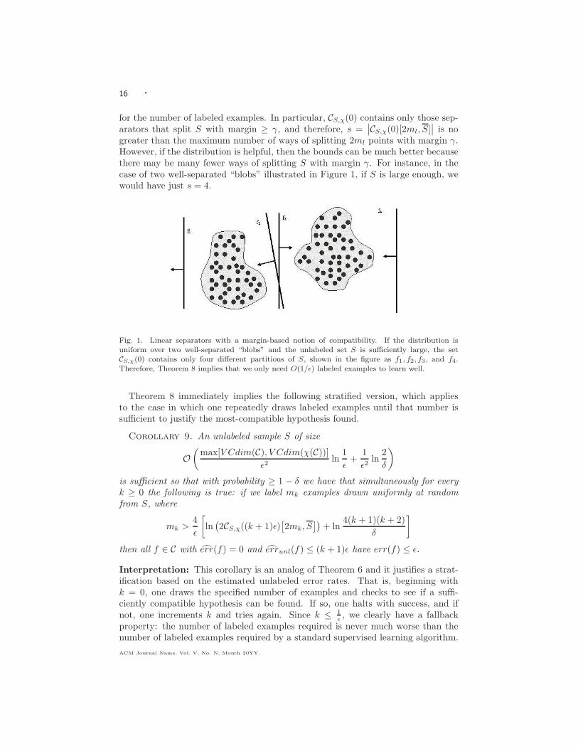
greater than the maximum number of ways of splitting 2ml points with margin γ.However, if the distribution is helpful, then the bounds can be much better becausethere may be many fewer ways of splitting S with margin γ. For instance, in thecase of two well-separated “blobs” illustrated in Figure 1, if S is large enough, wewould have just s = 4.

Fig. 1. Linear separators with a margin-based notion of compatibility. If the distribution isuniform over two well-separated “blobs” and the unlabeled set S is sufficiently large, the setCS,χ(0) contains only four different partitions of S, shown in the figure as f1, f2, f3, and f4.Therefore, Theorem 8 implies that we only need O(1/ǫ) labeled examples to learn well.

Theorem 8 immediately implies the following stratified version, which appliesto the case in which one repeatedly draws labeled examples until that number issufficient to justify the most-compatible hypothesis found.

Corollary 9. An unlabeled sample S of size

O(


ǫ2ln

1

ǫ+

1

ǫ2ln

2

δ

)

is sufficient so that with probability ≥ 1 − δ we have that simultaneously for everyk ≥ 0 the following is true: if we label mk examples drawn uniformly at randomfrom S, where

mk >4

ǫ

[ln

(2CS,χ((k + 1)ǫ)

[2mk, S

])+ ln

4(k + 1)(k + 2)

δ

]

then all f ∈ C with err(f) = 0 and errunl(f) ≤ (k + 1)ǫ have err(f) ≤ ǫ.

Interpretation: This corollary is an analog of Theorem 6 and it justifies a strat-ification based on the estimated unlabeled error rates. That is, beginning withk = 0, one draws the specified number of examples and checks to see if a suffi-ciently compatible hypothesis can be found. If so, one halts with success, and ifnot, one increments k and tries again. Since k ≤ 1

ǫ , we clearly have a fallbackproperty: the number of labeled examples required is never much worse than thenumber of labeled examples required by a standard supervised learning algorithm.


· 17

If one does not have the ability to draw additional labeled examples, then we canfix ml and instead stratify over estimation error as in [Bartlett et al. 1999]. Wediscuss this further in our agnostic bounds in Section 3.1.3 below.

3.1.3 The agnostic case. The bounds given so far have been based on the as-sumption that the target function belongs to C (so that we can assume there willexist f ∈ C with err(f) = 0). One can also derive analogous results for the agnostic(unrealizable) case, where we do not make that assumption. We first present oneimmediate bound of this form, and then show how we can use it in order to tradeoff labeled and unlabeled error in a near-optimal way. We also discuss the relationof this to a common regularization technique used in semi-supervised learning. Aswe will see, the differences between these two point to certain potential pitfalls inthe standard regularization approach.

Theorem 10. Let f∗t = argminf∈C [err(f)|errunl(f) ≤ t]. Then an unlabeled

sample S of size

O(


ǫ2ln

1

ǫ+

1

ǫ2ln

1

δ

)

and a labeled sample of size

ml ≥8

ǫ2

[ln

(CD,χ(t + 2ǫ)[2ml, D]

)+ ln

8

δ

]

is sufficient so that with probability ≥ 1− δ, the f ∈ C that optimizes err(f) subjectto errunl(f) ≤ t + ǫ has

err(f) ≤ err(f∗t ) + ǫ +

√ln(4/δ)/(2ml) ≤ err(f∗

t ) + 2ǫ.

Proof. The given unlabeled sample size implies that with probability 1 − δ/4,all f ∈ C have |errunl(f) − errunl(f)| ≤ ǫ, which also implies that errunl(f

∗t ) ≤

t + ǫ. The labeled sample size, using standard VC bounds (e.g, Theorem 26 in theAppendix D) imply that with probability at least 1− δ/2, all f ∈ CD,χ(t+2ǫ) haveerr(f)− err(f) ≤ ǫ. Finally, by Hoeffding bounds, with probability at least 1− δ/4we have

err(f∗t ) ≤ err(f∗

t ) +√

ln(4/δ)/(2ml).

Therefore, with probability at least 1 − δ, the f ∈ C that optimizes err(f) subjectto errunl(f) ≤ t + ǫ has

err(f) ≤ err(f) + ǫ ≤ err(f∗t ) + ǫ ≤ err(f∗

t ) + ǫ +√

ln(4/δ)/(2ml) ≤ err(f∗t ) + 2ǫ,

as desired.

Interpretation: Given a value t, Theorem 10 bounds the number of labeled ex-amples needed to achieve error at most ǫ larger than that of the best function f∗

t ofunlabeled error rate at most t. Alternatively, one can also state Theorem 10 in theform more commonly used in statistical learning theory: given any number of la-beled examples ml and given t > 0, Theorem 10 implies that with high probability,


18 ·the function f that optimizes err(f) subject to errunl(f) ≤ t + ǫ satisfies

err(f) ≤ err(f) + ǫt ≤ err(f∗t ) + ǫt +

√ln(4/δ)

2ml

where

ǫt =

√8

mlln

(8CD,χ(t + 2ǫ)[2ml, D]/δ

).

Note that as usual, there is an inherent tradeoff here between the quality of thecomparison function f∗

t , which improves as t increases, and the estimation error ǫt,which gets worse as t increases. Ideally, one would like to achieve a bound of

mint

[err(f∗t ) + ǫt] +

√ln(4/δ)/(2ml);

i.e., as if the optimal value of t were known in advance. We can perform nearlyas well as this bound by (1) performing a stratification over t (so that the boundholds simultaneously for all values of t) and (2) using an estimate ǫt of ǫt thatwe can calculate from the unlabeled sample and therefore use in the optimization.In particular, letting ft = argminf ′∈C[err(f ′) : errunl(f

′) ≤ t], we will outputf = argminft

[err(ft) + ǫt].Specifically, given a set S of unlabeled examples and ml labeled examples, let

ǫt = ǫt(S, ml) =

√24

mlln (8CS,χ(t)[ml, S]),

where we define CS,χ(t)[ml, S] to be the number of different partitions of the firstml points in S using functions in CS,χ(t), i.e., using functions of empirical unlabelederror at most t (we assume |S| ≥ ml). Then we have the following theorem.

Theorem 11. Let f∗t = argminf ′∈C [err(f ′)|errunl(f

′) ≤ t] and define ǫ(f ′) =ǫt′ for t′ = errunl(f

′). Then, given ml labeled examples, with probability at least1 − δ, the function

f = argminf ′ [err(f ′) + ǫ(f ′)]

satisfies the guarantee that

err(f) ≤ mint

[err(f∗t ) + ǫ(f∗

t )] + 5

√ln(8/δ)

ml.

Proof. First we argue that with probability at least 1 − δ/2, for all f ′ ∈ C wehave

err(f ′) ≤ err(f ′) + ǫ(f ′) + 4

√ln(8/δ)

ml.

In particular, define C0 = CS,χ(0) and inductively for k > 0 define Ck = CS,χ(tk) fortk such that Ck[ml, S] = 8Ck−1[ml, S]. (If necessary, arbitrarily order the functionswith empirical unlabeled error exactly tk and choose a prefix such that the sizecondition holds.) Also, we may assume without loss of generality that C0[ml, S] ≥ 1.


· 19

Then, using bounds of [Boucheron et al. 2000] (see also Appendix D), we have thatwith probability at least 1 − δ/2k+2, all f ′ ∈ Ck \ Ck−1 satisfy:

err(f ′) ≤ err(f ′) +

√6

mlln(Ck[ml, S]) + 4

√1

mlln(2k+3/δ)

≤ err(f ′) +

√6

mlln(Ck[ml, S]) + 4

√1

mlln(2k) + 4

√1

mlln(8/δ)

≤ err(f ′) +

√6

mlln(Ck[ml, S]) +

√6

mlln(8k) + 4

√1

mlln(8/δ)

≤ err(f ′) + 2

√6

mlln(Ck[ml, S]) + 4

√1

mlln(8/δ)

≤ err(f ′) + ǫ(f ′) + 4

√1

mlln(8/δ).

Now, let f∗ = argminf∗

t[err(f∗

t )+ ǫ(f∗t )]. By Hoeffding bounds, with probability at

least 1 − δ/2 we have err(f∗) ≤ err(f∗) +√

ln(2/δ)/(2ml). Also, by constructionwe have err(f) + ǫ(f) ≤ err(f∗) + ǫ(f∗). Therefore with probability at least 1− δwe have:

err(f) ≤ err(f) + ǫ(f) + 4√

ln(8/δ)/ml

≤ err(f∗) + ǫ(f∗) + 4√

ln(8/δ)/ml

≤ err(f∗) + ǫ(f∗) + 5√

ln(8/δ)/ml

as desired.

The above result bounds the error of the function f produced in terms of thequantity ǫ(f∗) which depends on the empirical unlabeled error rate of f∗. If ourunlabeled sample S is sufficiently large to estimate all unlabeled error rates to±ǫ, then with high probability we have errunl(f

∗t ) ≤ t + ǫ, so ǫ(f∗

t ) ≤ ǫt+ǫ,and moreover CS,χ(t + ǫ) ⊆ CD,χ(t + 2ǫ). So, our error term ǫ(f∗

t ) is at most√24ml

ln (8CD,χ(t + 2ǫ)[ml, S]). Recall that our ideal error term ǫt for the case that

t was given to the algorithm in advance, factoring out the dependence on δ, was√8

mlln

(8CD,χ(t + 2ǫ)[2ml, D]

). [Boucheron et al. 2000] show that for any class

C, the quantity ln(C[m, S]) is tightly concentrated about ln(C[m, D]) (see also The-orem 29 in the Appendix E), so up to multiplicative constants, these two boundsare quite close.

Interpretation and use of unlabeled error rate as a regularizer: The abovetheorem suggests to optimize the sum of the empirical labeled error rate plus anestimation-error bound (regularization function) based on the unlabeled error rate.A common related approach used in practice in machine learning (e.g., [Chapelleet al. 2006]) is to just directly optimize the sum of the two kinds of error: i.e.,to find argminf [err(f) + errunl(f)]. However, this is not generically justified inour framework, because the labeled and unlabeled error rates are really of different“types”. In particular, depending on the concept class and notion of compatibility,a small change in unlabeled error rate could substantially change the size of the


20 ·compatible set.6 For example, suppose all functions in C have unlabeled errorrate 0.6, except for two: function f0 has unlabeled error rate 0 and labeled errorrate 1/2, and function f0.5 has unlabeled error rate 0.5 and labeled error rate1/10. Suppose also that C is sufficiently large that with high probability it containssome functions f that drastically overfit, giving err(f) = 0 even though their trueerror is close to 1/2. In this case, we would like our algorithm to pick out f0.5

(since its labeled error rate is fairly low, and we cannot trust the functions ofunlabeled error 0.6). However, even if we use a regularization parameter λ, thereis no way to make f0.5 = argminf [err(f) + λerrunl(f)]: in particular, one cannothave 1/10 + 0.5λ ≤ min[1/2 + 0λ, 0 + 0.6λ]. So, in this case, this approach will nothave the desired behavior.

Application: A natural setting where we can efficiently apply the bounds of Theo-rem 11 is that of learning linear separators in a constant-dimensional space under amargin-based notion of compatibility. Given an unlabeled sample S, there are onlya polynomial number of partitions of S induced by the class C of linear separators,and for each one we can efficiently find the separator of highest compatibility. Thisin turn implies that by sampling, we can efficiently estimate the penalty term ǫt

for any given t, and therefore (again because C induces only a polynomial numberof distinct partitions of S) we can efficiently perform the argmin computation inTheorem 11. In Section 4.2 we demonstrate a more involved use of the boundsof Theorem 11 in a natural graph-based learning setting, where C induces an ex-ponential number of partitions of the dataset. Here, we are able to find a goodupper bound on the penalty term ǫ(f) which can be easily computed and has anice functional form. Moreover, because of this form, we can efficiently performthe argmin computation solving for the hypothesis of smallest empirical error pluspenalty, without needing to use a surrogate loss for the empirical error term as isoften done in cases of large hypothesis spaces. See Section 4.2.

Fallback Guarantees: We end this section with a corollary pointing out that ifwe have a purely supervised regularization function, we can combine that with thecompatibility-based bound of Theorem 11 to perform nearly as well as the best ofthe two.

Corollary 12. Suppose λ(f) is a regularization function such that given ml

labeled examples, with probability at least 1 − δ the hypothesis

f = argminf ′ [err(f ′) + λ(f ′)]

satisfies

err(f) ≤ minf ′

[err(f ′) + λ(f ′)] + g(ml, δ)

for some function g. Also let h(m, δ) = 5√

ln(8/δ)/m. Then with probability atleast 1 − 2δ, the hypothesis

f = argminf ′ [ err(f ′) + min[ǫ(f ′) + h(ml, δ), λ(f ′) + g(ml, δ)] ]

satisfies err(f) ≤ minf ′ [err(f ′) + min[ǫ(f ′) + h(ml, δ), λ(f ′) + g(ml, δ)]].

6On the other hand, for certain compatibility notions and under certain natural assumptions, onecan use unlabeled error rate directly, e.g., see e.g., [Sridharan and Kakade 2008].


· 21

Note that one could also derive bounds based on other distribution dependentcomplexity measures and using other concentration results (see e.g. [Boucheronet al. 2005]).

3.2 ǫ-Cover-based Bounds

The results in the previous section are uniform convergence bounds: they provideguarantees for any algorithm that optimizes over the observed data. In this section,we consider stronger bounds based on ǫ-covers that apply to algorithms that behavein a specific way: they first use the unlabeled examples to choose a “representative”set of compatible hypotheses, and then use the labeled sample to choose amongthese. Bounds based on ǫ-covers exist in the classical PAC setting, but in ourframework these bounds and algorithms of this type are especially natural, and thebounds are often much lower than what can be achieved via uniform convergence.For simplicity, we restrict ourselves in this section to the realizable case. Howeverone can combine ideas in Section 3.1.3 with ideas in this section in order to derivebounds in the agnostic case as well. We first present our generic bounds. InSection 3.2.1 we discuss natural settings in which they can be especially useful, andin then Section 3.2.2 we present even tighter bounds for co-training.

Recall that a set Cǫ ⊆ 2X is an ǫ-cover for C with respect to D if for every f ∈ Cthere is a f ′ ∈ Cǫ which is ǫ-close to f . That is, Prx∼D(f(x) 6= f ′(x)) ≤ ǫ.

Theorem 13. Assume c∗ ∈ C and let p be the size of a minimum ǫ-cover forCD,χ(errunl(c

∗) + 2ǫ). Then using mu unlabeled examples and ml labeled examplesfor

mu = O(


ǫ2ln

1

ǫ+

1

ǫ2ln

2

δ

)and ml = O

(1

ǫln

p

δ

),

we can with probability 1 − δ identify a hypothesis f ∈ C with err(f) ≤ 6ǫ.

Proof. Let t = errunl(c∗). Now, given the unlabeled sample SU , define C′ ⊆ C

as follows: for every labeling of SU that is consistent with some f in C, choose a hy-pothesis in C for which errunl(f) is smallest among all the hypotheses correspondingto that labeling. Next, we obtain Cǫ by eliminating from C′ those hypotheses fwith the property that errunl(f) > t + ǫ. We then apply a greedy procedure on Cǫ

to obtain Gǫ = g1, · · · , gs, as follows:Initialize C1

ǫ = Cǫ and i = 1.

(1) Let gi = argminf∈Ci

ǫ

errunl(f).

(2) Using the unlabeled sample SU , determine Ci+1ǫ by deleting from Ci

ǫ those

hypotheses f with the property that d(gi, f) < 3ǫ.

(3) If Ci+1ǫ = ∅ then set s = i and stop; else, increase i by 1 and goto 1.

We now show that with high probability, Gǫ is a 5ǫ-cover of CD,χ(t) with respectto D and has size at most p. First, our bound on mu is sufficient to ensure thatwith probability ≥ 1 − δ

2 , we have (a) |d(f, g) − d(f, g)| ≤ ǫ for all f, g ∈ C and (b)|errunl(f) − errunl(f)| ≤ ǫ for all f ∈ C. Let us assume in the remainder that this(a) and (b) are indeed satisfied. Now, (a) implies that any two functions in C thatagree on SU have distance at most ǫ, and therefore C′ is an ǫ-cover of C. Using


22 ·(b), this in turn implies that Cǫ is an ǫ-cover for CD,χ(t). By construction, Gǫ is a3ǫ-cover of Cǫ with respect to distribution SU , and thus (using (a)) Gǫ is a 4ǫ-coverof Cǫ with respect to D, which implies that Gǫ is a 5ǫ-cover of CD,χ(t) with respectto D.

We now argue that Gǫ has size at most p. Fix some optimal ǫ-cover f1, . . . , fpof CD,χ(errunl(c

∗) + 2ǫ). Consider function gi and suppose that gi is covered byfσ(i). Then the set of functions deleted in step (2) of the procedure include thosefunctions f satisfying d(gi, f) < 2ǫ which by triangle inequality includes thosesatisfying d(fσ(i), f) ≤ ǫ. Therefore, the set of functions deleted include thosecovered by fσ(i) and so for all j > i, σ(j) 6= σ(i); in particular, σ is 1-1. Thisimplies that Gǫ has size at most p.

Finally, to learn c∗ we simply output the function f ∈ Gǫ of lowest empirical errorover the labeled sample. By Chernoff bounds, the number of labeled examples isenough to ensure that with probability ≥ 1 − δ

2 the empirical optimum hypothesisin Gǫ has true error at most 6ǫ. This implies that overall, with probability ≥ 1− δ,we find a hypothesis of error at most 6ǫ.

Note that Theorem 13 relies on knowing a good upper bound on errunl(c∗). If

we do not have such an upper bound, then one can perform a stratification asin Sections 3.1.2 and 3.1.3. For example, if we have a desired maximum errorrate ǫ and we do not know a good upper bound for errunl(c

∗) but we have theability to draw additional labeled examples as needed, then we can simply run theprocedure in Theorem 13 for various values of p, testing on each round to see ifthe hypothesis f found indeed has zero empirical labeled error rate. One can showthat ml = O

(1ǫ ln p

δ

)labeled examples are sufficient in total for all the “validation”

steps.7 If the number of labeled examples ml is fixed, then one can also perform astratification over the target error ǫ.

3.2.1 Some illustrative examples. To illustrate the power of ǫ-cover bounds, wenow present two examples where these bounds allow for learning from significantlyfewer labeled examples than is possible using uniform convergence.

Graph-based learning: Consider the setting of graph-based algorithms (e.g.,Example 3). In particular, the input is a graph G where each node is an exampleand C is the class of all boolean functions over the nodes of G. Let us define theincompatibility of a hypothesis to be the fraction of edges in G cut by it. Supposenow that the graph G consists of two cliques of n/2 vertices, connected together byǫn2/4 edges. Suppose the target function c∗ labels one of the cliques as positiveand one as negative, so the target function indeed has unlabeled error rate less thanǫ. Now, given any set SL of ml < ǫn/4 labeled examples, there is always a highly-compatible hypothesis consistent with SL that just separates the positive pointsin SL from the entire rest of the graph: the number of edges cut will be at mostnml < ǫn2/4. However, such a hypothesis has true error nearly 1/2 since it has

7Specifically, note that as we increase t (our current estimate for the unlabeled error rate of thetarget function), the associated p (which is an integer) increases in discrete jumps, p1, p2, . . .. Wecan then simply spread the “δ” parameter across the different runs, in particular run i would useδ/i(i + 1). Since pi ≥ i, this implies that ml = O

`

1ǫ

ln pδ

´

labeled examples are sufficient for allthe “validation” steps.


· 23

less than ǫn/4 positive examples. So, we do not yet have uniform convergence overthe space of highly compatible hypotheses, since this hypothesis has zero empiricalerror but high true error. Indeed, this illustrates an overfitting problem that canoccur with a direct minimum-cut approach to learning [Blum and Chawla 2001;Joachims 2003; Blum et al. 2004]. On the other hand, the set of functions ofunlabeled error rate less than ǫ has a small ǫ-cover: in particular, any partition ofG that cuts less than ǫn2/4 edges must be ǫ-close to (a) the all-positive function,(b) the all-negative function, (c) the target function c∗, or (d) the complement ofthe target function 1− c∗. So, ǫ-cover bounds act as if the concept class had only 4functions and so by Theorem 13 we need only O(1

ǫ ln 1δ ) labeled examples to learn

well.8 (In fact, since the functions in the cover are all far from each other, we reallyneed only O(ln 1

δ ) examples. This issue is explored further in Theorem 15).

Simple co-training: For another case where ǫ-cover bounds can beat uniform-convergence bounds, imagine examples are pairs of points in 0, 1d, C is the classof linear separators, and compatibility is determined by whether both points areon the same side of the separator (i.e., the case of Example 4). Now suppose forsimplicity that the target function just splits the hypercube on the first coordinate,and the distribution is uniform over pairs having the same first coordinate (so thetarget is fully compatible). We then have the following.

Theorem 14. Given poly(d) unlabeled examples SU and 14 log2 d labeled exam-

ples SL, with high probability there will exist functions of true error 1/2 − 2−12

√d

that are consistent with SL and compatible with SU .

Proof. Let V be the set of all variables (not including x1) that (a) appear inevery positive example of SL and (b) appear in no negative example of SL. In otherwords, these are variables xi such that the function f(x) = xi correctly classifiesall examples in SL. Over the draw of SL, each variable has a (1/2)2|SL| = 1/

√d

chance of belonging to V , so the expected size of V is (d−1)/√

d and so by Chernoffbounds, with high probability V has size at least 1

2

√d. Now, consider the hypothesis

corresponding to the conjunction of all variables in V . This correctly classifies theexamples in SL, and with probability at least 1−2|SU |2−|V | it classifies every otherexample in SU negative because each example in SU has only a 1/2|V | chance ofsatisfying every variable in V . Since |SU | = poly(d), this means that with highprobability this conjunction is compatible with SU and consistent with SL, even

though its true error is at least 1/2 − 2−12

√d.

So, given only a set SU of poly(d) unlabeled examples and a set SL of 14 log2 d

labeled examples we would not want to use a uniform convergence based algorithmsince we do not yet have uniform convergence. In contrast, the cover-size of the setof functions compatible with SU is constant, so ǫ-cover based bounds again allowlearning from just only O(1

ǫ ln 1δ ) labeled examples (Theorem 13). In fact as we

show in Theorem 15 we only need O(log 1

ǫ

1δ

)labeled examples in this case.

8Effectively, ǫ-cover bounds allow one to rule out a hypothesis that, say, just separates the positivepoints in SL from the rest of the graph by noting that this hypothesis is very close (with respectto D) to the all-negative hypothesis, and that hypothesis has a high labeled-error rate.


24 ·3.2.2 Learning from even fewer labeled examples. In some cases, unlabeled data

can allow us to learn from even fewer labeled examples than given by Theorem 13.In particular, consider a co-training setting where the target c∗ is fully compatibleand D satisfies the property that the two views x1 and x2 are conditionally inde-pendent given the label c∗(〈x1, x2〉). As shown by [Blum and Mitchell 1998], onecan boost any weak hypothesis from unlabeled data in this setting (assuming onehas enough labeled data to produce a weak hypothesis). Related sample complexityresults are given in [Dasgupta et al. 2001]. In fact, we can use the notion of ǫ-coversto show that we can learn from just a single labeled example. Specifically, for anyconcept classes C1 and C2, we have:

Theorem 15. Assume that err(c∗) = errunl(c∗) = 0 and D satisfies indepen-

dence given the label. Then for any τ ≤ ǫ/4, using mu unlabeled examples and ml

labeled examples we can find a hypothesis that with probability 1 − δ has error atmost ǫ, for

mu = O(

1

τ

[(V Cdim(C1) + V Cdim(C2)) ln

1

τ+ ln

2

δ

])and ml = O

(log 1

τ

1

δ

).

Proof. We will assume for simplicity the setting of Example 3, where c∗ = c∗1 =c∗2 and also D1 = D2 = D (the general case is handled similarly, but just requiresmore notation).

We start by characterizing the hypotheses with low unlabeled error rate. Recallthat χ(f, D) = Pr〈x1,x2〉∼D[f(x1) = f(x2)], and for concreteness assume f predictsusing x1 if f(x1) 6= f(x2). Consider f ∈ C with errunl(f) ≤ τ and let us definep− = Prx∈D [c∗(x) = 0], p+ = Prx∈D [c∗(x) = 1] and for i, j ∈ 0, 1 define pij =Prx∈D [f(x) = i, c∗(x) = j]. We clearly have err (f) = p10 +p01. From errunl(f) =Pr(x1,x2)∼D [f (x1) 6= f (x2)] ≤ τ , using the independence given the label of D, weget

2p10p00

p10 + p00+

2p01p11

p01 + p11≤ τ.

In particular, the fact that 2p10p00

p10+p00≤ τ implies that we cannot have both p10 > τ

and p00 > τ , and the fact that 2p01p11

p01+p11≤ τ implies that we cannot have both

p01 > τ and p11 > τ . Therefore, any hypothesis f with errunl(f) ≤ τ falls in oneof the following categories:

(1) f is “close to c∗”: p10 ≤ τ and p01 ≤ τ ; so err(f) ≤ 2τ .

(2) f is “close to c∗”: p00 ≤ τ and p11 ≤ τ ; so err(f) ≥ 1 − 2τ .

(3) f “almost always predicts negative”: for p10 ≤ τ and p11 ≤ τ ; so Pr[f(x) =0] ≥ 1 − 2τ .

(4) f “almost always predicts positive”: for p00 ≤ τ and p01 ≤ τ ; so Pr[f(x) =0] ≤ 2τ .

Let f1 be the constant positive function and f0 be the constant negative function.Now note that our bound on mu is sufficient to ensure that with probability ≥ 1− δ

2 ,

we have (a) |d(f, g)−d(f, g)| ≤ τ for all f, g ∈ C and (b) all f ∈ C with errunl(f) = 0satisfy errunl(f) ≤ τ . Let us assume in the remainder that this (a) and (b) areindeed satisfied. By our previous analysis, there are at most four kinds of hypotheses


· 25

consistent with unlabeled data: those close to c∗, those close to its complementc∗, those close to f0, and those close to f1. Furthermore, c∗, c∗, f0, and f1 arecompatible with the unlabeled data.

So, algorithmically, we first check to see if there exists a hypothesis g ∈ C witherrunl(g) = 0 such that d(f1, g) ≥ 3τ and d(f0, g) ≥ 3τ . If such a hypothesis gexists, then it must satisfy either case (1) or (2) above. Therefore, we know thatone of g, g is 2τ -close to c∗. If not, we must have p+ ≤ 4τ or p− ≤ 4τ , in whichcase we know that one of f0, f1 is 4τ -close to c∗. So, either way we have a set oftwo functions, opposite to each other, one of which is at least 4τ -close to c∗. Wefinally use O(log 1

τ

1δ ) labeled examples to pick one of these to output, namely the

one with lowest empirical labeled error. Lemma 16 below then implies that withprobability 1 − δ the function we output has error at most 4τ ≤ ǫ.

Lemma 16. Consider τ < 18 . Let Cτ =

f, f

be a subset of C containing two

opposite hypotheses with the property that one of them is τ-close to c∗. Then,ml > 6 log( 1

τ )(

1δ

)labeled examples are sufficient so that with probability ≥ 1 − δ,

the concept in Cτ that is τ-close to c∗ in fact has lower empirical error.

Proof. See Appendix E.

In particular, by reducing τ to poly(δ) in Theorem 15, we can reduce the numberof labeled examples needed ml to one. Note however that we will need polynomiallymore unlabeled examples.

In fact, the result in Theorem 15 can be extended to the case that D+ and D−

merely satisfy constant expansion rather than full independence given the label, see[Balcan et al. 2004].

Note: Theorem 15 illustrates that if data is especially well behaved with respect tothe compatibility notion, then our bounds on labeled data can be extremely good.In Section 4.3, we show for the case of linear separators and independence given thelabel, we can give efficient algorithms, achieving the bounds in Theorem 15 in termsof labeled examples by a polynomial time algorithm. Note, however, that both thesebounds rely heavily on the assumption that the target is fully compatible. If theassumption is more of a “hope” than a belief, then one would need an additionalsample of 1/ǫ labeled examples just to validate the hypothesis produced.

4. ALGORITHMIC RESULTS

In this section we give several examples of efficient algorithms in our model thatare able to take advantage of unlabeled data and learn using sample sizes com-parable to those described in Section 3. We begin in Section 4.1 by consideringthe problem of learning disjunctions in the doubly realizable case for a simplecompatibility notion, presenting an algorithm achieving the sample-size bounds inSection 3.1.1. Next in Section 4.2 we give a more interesting example showing howwe can efficiently perform data dependent structural risk minimization in a naturaltransductive graph-based learning setting, illustrating the bounds of Section 3.1.3.Finally, in section 4.3 we present a new efficient algorithm for Co-Training withlinear separators that, if the distribution satisfies independence given the label, re-quires only a single labeled example to learn to any desired error rate ǫ, matchingthe ǫ-cover labeled sample bounds in Section 3.2.


26 ·Note that our focus is on achieving a low-error hypothesis (also called minimizing

0-1 loss). Another common practice in machine learning (both for supervised andsemi-supervised learning) is to instead try to minimize a surrogate convex lossthat is easier to optimize [Chapelle et al. 2006]. While this does simplify thecomputational problem, it does not in general solve the true goal of achieving lowerror since in general the minimizer of the surrogate loss can have a large 0-1 loss.

4.1 An efficient semi-supervised algorithm for disjunctions

We give here a simple example to illustrate the bounds in Section 3.1.1, and forwhich we can give a polynomial-time algorithm that takes advantage of them. Letthe instance space X = 0, 1d, and for x ∈ X , let vars(x) be the set of variablesset to 1 by x. Let C be the class of monotone disjunctions (e.g., x1 ∨ x3 ∨ x6),and for f ∈ C, let vars(f) be the set of variables disjoined by f . Now, suppose wesay an example x is compatible with function f if either vars(x) ⊆ vars(f) or elsevars(x) ∩ vars(f) = φ. This is a very strong notion of “margin”: it says, in essence,that every variable is either a positive indicator or a negative indicator, and noexample should contain both positive and negative indicators.

We assume the “doubly realizable” case where we assume c∗ ∈ C and errunl(c∗) =

0. Given this setup, we can give a simple learning algorithm for this pair (C, χ)with sample size bounds matching those in Theorem 4. Specifically, we prove:

Theorem 17. The class C of monotone disjunctions is learnable in polynomialtime under the compatibility notion defined above with sample size bounds matchingthose in Theorem 4.

Proof. We begin by using our unlabeled data to construct a graph on d vertices(one per variable), putting an edge between two vertices i and j if there is anyexample x in our unlabeled sample with i, j ∈ vars(x). We now use our labeleddata to label the components. If the target function is fully compatible, then nocomponent will get multiple labels (if some component does get multiple labels,we halt with failure). Finally, we produce the hypothesis f such that vars(f) isthe union of the positively-labeled components. This is fully compatible with theunlabeled data and has zero error on the labeled data, so by Theorem 4, if the sizesof the data sets are as given in the bounds, with high probability the hypothesisproduced will have error at most ǫ.

Notice that if we want to view the algorithm as “purchasing” labeled data, thenwe can simply examine the graph, count the number of connected components k,and then request 1

ǫ [k ln 2 + ln 2δ ] labeled examples. (Here, 2k = |CS,χ(0)|.) By the

proof of Theorem 4, with high probability 2k ≤ |CD,χ(ǫ)|, so we are purchasing nomore than the number of labeled examples in the theorem statement.

Also, it is interesting to see the difference between a “helpful” and “non-helpful”distribution for this problem. An especially non-helpful distribution would be theuniform distribution over all examples x with |vars(x)| = 1, in which there are dcomponents. In this case, unlabeled data does not help at all, and one still needsΩ(d) labeled examples (or, even Ω

(dǫ

)if the distribution is non-uniform as in the

lower bounds of [Ehrenfeucht et al. 1989]). On the other hand, a helpful distributionis one such that with high probability the number of components is small, such asthe case of features appearing independently given the label.


· 27

For the semi-agnostic case, where c∗ ∈ C but errunl(c∗) > 0, the natural approach

would be to solve for the consistent hypothesis of minimum unlabeled error over S.Unfortunately, as shown in Appendix C, this problem is NP-hard. A different prob-lem where one can efficiently solve for the most-compatible consistent hypothesisis graph-based learning with a cut-size compatibility notion. Indeed, this is whatis done by the min-cut learning algorithm of [Blum and Chawla 2001]. In fact, forthis problem one can even do a full data-dependent structural risk minimization,and we describe this in Section 4.2 below.

4.2 Efficient structural risk minimization for graph-based learning

We show here how we can apply the bounds of Theorem 11 in a natural graph-basedlearning setting to yield an efficient algorithm for structural risk minimization. In-terestingly, in this setting not only do we have a good upper bound on the penaltyterm ǫ(f) with a nice functional form, but also because of this form, we can ef-ficiently solve for the hypothesis of smallest empirical error plus penalty, withoutneeding to use a surrogate loss for the empirical error term. This allows us to effi-ciently achieve an agnostic PAC guarantee, getting error nearly as good as the bestfunction of any given compatibility level, with a gap that degrades gracefully withthe degree of incompatibility and the number of labeled examples.

We assume our input is an unweighted graph G over the dataset S. This is atransductive problem (see also Section 5.1): S is fixed and our goal is to do well withrespect to the uniform distribution over S. Our hypothesis class C consists of all2|S| labelings of S, and we consider a cut-size notion of compatibility. Specifically,we define errunl(f) to be the fraction of edges in G whose endpoints are assigneddifferent labels by f (i.e., the fraction of edges cut by f). For ease of discussion,we assume that G is connected, so the only hypotheses of perfect compatibility arethe all-positive and all-negative labelings. Given a random labeled subset of S, ourgoal in applying Theorem 11 is to identify the hypothesis f minimizing the sumof its empirical labeled error err(f) and the regularization term ǫ(f). We showhere how for this problem we can produce a good bound on ǫ(f), and moreover wecan identify the desired hypothesis efficiently, yielding an efficient well-motivatedregularized semi-supervised learning algorithm. Specifically, we use Theorem 11 toprove the following result. Let tmin be the fraction of edges cut by the minimumnontrivial cut in G.

Theorem 18. If G has a partition of true error α and cutting a t fraction ofedges, then there exists an efficient algorithm that with probability at least 1 − δ

produces a hypothesis f of error at most α + O

(√(1+t/tmin) ln(ml/δ)

ml

).

Proof. Algorithmically, to use Theorem 11 we have two tasks. The first is tocalculate or determine a good upper bound on the regularization term ǫ(f), andthe second is to efficiently find argminf [err(f) + ǫ(f)], where ǫ(f) is our computedupper-bound on ǫ(f). (Note that if we required err(f) = 0, i.e. perfect behavioron the given labeled data, we could easily compute the hypothesis minimizingǫ(f) by collapsing the labeled positive and negative examples into a source andsink respectively and solving for the minimum cut. However, we instead want toperform a tradeoff.)


28 ·For the first task, we can use results of Kleinberg et al. [Kleinberg 2000; Kleinberg

et al. 2004] showing that for any connected graph G, the VC-dimension of the setof partitions of unlabeled error rate at most t is O(1 + t/tmin) where tmin is thefraction of edges cut by the minimum nontrivial cut in G.9 Therefore, by Sauer’slemma this implies that

ln (CS,χ(t)[ml, S]) = ln(mO(1+t/tmin)l ) = O((1 + t/tmin) lnml).

Notice that this is a graph-dependent quantity since tmin is a function of the graph

G. We define ǫ(f) = O(√

(1 + t/tmin) ln(ml)/ml

)to be the quantity ǫ(f) pro-

duced using this upper bound.For the second task, we need to compute the function f minimizing empirical

error plus our estimation error bound. For this we can use the following approach.First, connect a source vs to all labeled positive examples via edges of weight 1, asink vt to all labeled negative examples via edges of weight 1, and assign each edgein G a weight of λ. If we now find the minimum vs-vt cut, this will produce thefunction fλ minimizing the number of labeled mistakes plus λ times the numberof unlabeled mistakes (edges cut in G). Unfortunately, our estimation error boundǫ(f) is not a linear function of the number of unlabeled mistakes so we cannotdirectly convert it to a scalar λ. However, it is a concave function, which meansthat the argmin of err(f) + ǫ(f) must be the minimizer of err(f) + λ∗errunl(f)for some value λ∗ (see Lemma 19 below). Therefore, we can scan through valuesof λ to determine all distinct functions fλ produced (there are at most ml + 1 suchfunctions since each will have at least one more labeled mistake than the previous)and then output the argmin among these.

Thus, we can use this approach to efficiently solve for our desired hypothesis.This completes the proof.

Lemma 19. Let S = (x1, y1), . . . , (xn, yn) ⊂ R2, and let g(y) be a concaveincreasing function. Then the point (xi, yi) ∈ S minimizing x + g(y) must be thepoint in S minimizing x + λy for some λ > 0.

Proof. Let S′ ⊆ S be the set of points in S that minimize x + λy for someλ > 0. Then S′ is exactly the points (xk, yk) on the convex hull of S such that for allj 6= k, either xj > xk or yj > yk. Now, suppose (xi, yi) is the point in S minimizingx + g(y). Then clearly there cannot be (xj , yj) 6= (xi, yi) such that xj ≤ xi andyj ≤ yi because then xj + g(yj) < xi + g(yi) since g is an increasing function.Furthermore, (xi, yi) must be on the convex hull of S. In particular, suppose not.Then there must be some (xj , yj), (xk, yk) ∈ S with xi = αxj + (1 − α)xk forα ∈ [0, 1] but yi > αyj + (1 − α)yk. In that case we have

xi + g(yi) > αxj + (1 − α)xk + g(αyj + (1 − α)yk)

≥ αxj + (1 − α)xk + αg(yj) + (1 − α)g(yk)

≥ min(xj + g(yj), xk + g(yk)),

9Typically one would state this using t and tmin as the number of edges cut rather than thefraction, but we will normalize both here (which doesn’t affect their ratio) to be consistent withthe terminology used throughout this paper.


· 29

where the first “≥” follows from concavity of g. This in turn contradiction thedefinition of (xi, yi). Therefore, (xi, yi) must minimize x + λy for some λ > 0.

4.3 Co-training with linear separators: an efficient cover based algorithm

In this section we consider the problem of learning the class C of linear separa-tors under the Co-training compatibility notion, in the doubly-realizable case. Forsimplicity we focus first on the case of Example 4: the target function is a linearseparator in Rd and each example is a pair of points, both of which are assumed tobe on the same side of the separator (i.e., an example is a line-segment that doesnot cross the target hyperplane). We then show how our results can be extendedto the more general setting.

Unfortunately, unlike the previous examples, the consistency problem here evenwith double realizability is NP-hard: given a graph G embedded in Rd with twodistinguished points s and t, it is NP-hard to find the linear separator with s onone side and t on the other that cuts the minimum number of edges, even if theminimum is zero [Flaxman 2003]. For this reason, we will make an additional as-sumption, that the two points in an example are each drawn independently giventhe label. That is, there is a single distribution D over Rd, and with some proba-bility p+, two points are drawn i.i.d. from D+ (D restricted to the positive side ofthe target function) and with probability 1 − p+, the two are drawn i.i.d from D−(D restricted to the negative side of the target function). Note that our samplecomplexity results in Section 3.2 extend to weaker assumptions such as distribu-tional expansion introduced by [Balcan et al. 2004], but we need true independencefor our algorithmic results. [Blum and Mitchell 1998] also give positive algorithmicresults for co-training when (a) the two views of an example are drawn indepen-dently given the label (which we are assuming now), (b) the underlying functionis learnable via Statistical Query algorithms10 (which is true for linear separators[Blum et al. 1998]), and (c) we have enough labeled data to produce a weakly-usefulhypothesis (defined below) on one of the views to begin with. We give here an im-provement over that result by showing how we can run the algorithm in [Blumand Mitchell 1998] with only a single labeled example, thus obtaining an efficientalgorithm in our model. It is worth noticing that in the process, we also somewhatsimplify the results of [Blum et al. 1998] on efficiently learning linear separatorswith noise without a margin assumption.

For the analysis below, we need the following definition. A weakly-useful predictoris a function f such that for some β that is at least inverse polynomial in the inputsize we have:

Pr[f(x) = 1|c∗(x) = 1] > Pr[f(x) = 1|c∗(x) = 0] + β. (2)

It is equivalent to the usual notion of a “weak hypothesis” [Kearns and Vazirani1994] when the target function is balanced, but requires the hypothesis give moreinformation when the target function is unbalanced [Blum and Mitchell 1998]. Also,we will assume for convenience that the target separator passes through the origin,and let us denote the separator by c∗ · x = 0.

10For a detailed description of the Statistical Query model see [Kearns 1998] and [Kearns andVazirani 1994].


30 ·We now describe an efficient algorithm to learn to any desired error rate ǫ in

this setting from just a single labeled example. For clarity, we first describe analgorithm whose running time depends polynomially on both the dimension d and1/γ, where γ is a soft margin of separation between positive and negative examples.Formally, in this case we assume that at least some non-negligible probability massof examples x satisfy

|x · c∗||x||c∗| ≥ γ.

I.e., they have distance at least γ to the separating hyperplane x · c∗ = 0 afternormalization. This is a common type of assumption in machine learning (in fact,often one makes the much stronger assumption that nearly all probability mass ison examples x satisfying this condition). We then show how one can replace thedependence on 1/γ with instead a polynomial dependence on the number of bitsof precision b in the data, using the Outlier Removal Lemma of [Blum et al. 1998]and [Dunagan and Vempala 2001].

Algorithm 1 Co-training with Linear Separators. The Soft Margin Case.

Input: ǫ, δ, T , a set SL of ml labeled examples drawn i.i.d from D, a set SU

of mu unlabeled examples drawn i.i.d from D.

Let hp be the all-positive function. Let hn be the all-negative function.Let τ = ǫ/6, ǫ1 = τ/4.

(1) For i = 1, . . . , T do- Choose a random halfspace fi going through the origin.- Feed fi, SU , the error parameters ǫ1, and the confidence parameter δ/6

into the bootstrapping procedure of [Blum and Mitchell 1998] to producehypothesis hi.

(2) Let h be argminhi

errunl(hi)|d(h, hp) ≥ 3τ, d(h, hn) ≥ 3τ

.

If errunl(hi) ≥ 3ǫ1, then let h = hp.

(3) Use SL to output either h or h: output the hypothesis with lowest empiricalerror on the set SL.

Theorem 20. Assume that at least an α probability mass of examples x have

margin |x·c∗||x||c∗| ≥ γ with respect to the target separator c∗. There is a polynomial-

time algorithm (polynomial in d, 1/γ, 1/α, 1/ǫ, and 1/δ) to learn a linear separatorunder the above assumptions to error rate ǫ with probability 1−δ, from a polynomialnumber of unlabeled examples and a single labeled example.

Proof. Let ǫ and δ be the desired accuracy and confidence parameters. Let T =

O(

1α·γ ln

(1δ

)), mu = poly(1/γ, 1/α, 1/ǫ, 1/δ, d), and ml = 1. We run Algorithm 1

with the inputs ǫ, δ, T SL, SU , and ml = 1. Let τ = ǫ/6, ǫ1 = τ/4.In order to prove the desired result, we start with a few facts.


· 31

We first note that our bound on mu is sufficient to ensure that with probability≥ 1 − δ

3 , we have (a) |d(f, g) − d(f, g)| ≤ τ for all f, g ∈ C and (b) all f ∈ C have|errunl(f) − errunl(f)| ≤ ǫ1.

We now argue that if at least an α probability mass of examples x have margin|x·c∗||x||c∗| ≥ γ with respect to the target separator c∗, then a random halfspace has at

least a poly(α, γ) probability of being a weakly-useful predictor. (Note that [Blumet al. 1998] uses the Perceptron algorithm to get weak learning; here, we needsomething simpler since we need to save our labeled example to the very end.)Specifically, consider a point x of margin γx ≥ γ. By definition, the margin is thecosine of the angle between x and c∗, and therefore the angle between x and c∗ is

π/2 − cos−1(γx) ≤ π/2 − γ.

Now, imagine that we draw f at random subject to f · c∗ ≥ 0 (half of the f ’s willhave this property) and define f(x) = sign(f · x). Then,

Prf (f(x) 6= c∗(x)|f · c∗ ≥ 0) ≤ (π/2 − γ)/π = 1/2 − γ/π.

Moreover, if x does not have margin γ then at the very least we have Prf (f(x) 6=c∗(x)|f · c∗ ≥ 0) ≤ 1/2.

Now define distribution D∗ = 12D+ + 1

2D−; that is D∗ is the distribution D butbalanced to 50% positive and 50% negative. With respect to D∗ at least an α/2probability mass of the examples have margin at least γ, and therefore:

Ef [errD∗(f)|f · c∗ ≥ 0] ≤ 1/2 − (α/2)(γ/π).

Since err(f) is a bounded quantity, by Markov inequality this means that at leastan Ω(αγ) probability mass of functions f must satisfy

errD∗(f) ≤ 1

2− αγ

4π

which in turn implies that they must be useful weakly predictors with respect toD as defined in Equation (2) with β = αγ

4π .The second part of the argument is as follows. Note that in Step(1) of our algo-

rithm we repeat the following process for T iterations: pick a random fi, and plugit into the bootstrapping theorem of [Blum and Mitchell 1998] (which, given a dis-tribution over unlabeled pairs 〈xj

1, xj2〉, will use fi(x

j1) as a noisy label of xj

2, feeding

the result into a Statistical Query algorithm). Since T = O(

1α·γ ln

(1δ

)), using the

above observation about random halfspaces being weak predictors, we obtain thatwith high probability at least 1 − δ/6, at least one of the random hypothesis fi

was a weakly-useful predictor; and since mu = poly(1/γ, 1/α, 1/ǫ, 1/δ, d) we alsohave the associated hypothesis hi output by the bootstrapping procedure of [Blumand Mitchell 1998] will with probability at least 1 − δ/6 satisfy err(hi) ≤ ǫ1. Thisimplies that with high probability at least 1 − 2δ/3, at least one of the hypothesishi we find in Step 1 has true labeled error at most ǫ1. For the rest of the hypotheseswe find in Step 1, we have no guarantees.

We now observe the following. First of all, any function f with small err(f) musthave small errunl(f); in particular,

errunl(f) = Pr(f(x1) 6= f(x2)) ≤ 2err(f).


32 ·This implies that with high probability at least 1−2δ/3, at least one of the hypothe-sis hi we find in Step 1 has true unlabeled error at most 2ǫ1, and therefore empiricalunlabeled error at most 3ǫ1. Secondly, because of the assumption of independencegiven the label, as shown in Theorem 15, with high probability the only functionswith unlabeled error at most τ are functions 2τ -close to c∗, 2τ -close to ¬c∗, 2τ -closeto the “all positive” function, or 2τ -close to the “all negative” function.

In Step (2) we first examine all the hypotheses produced in Step 1, and we pickthe hypothesis h with the smallest empirical unlabeled error rate subject to beingempirically at least 3τ -far from the “all-positive” or “all-negative” functions. If thethe empirical error rate of this hypothesis h is at most 3ǫ1 we know that its trueunlabeled error rate is at most 4ǫ1 ≤ τ , which further implies that either h or ¬his 2τ close to c∗. However, if the empirical unlabeled error rate of h is greater than3ǫ1, then we know that the target must be 4τ -close to the all-positive or all-negativefunction so we simply choose h = “all positive” (this is true since the unlabeled

sample was large enough so that |d(f, g) − d(f, g)| ≤ τ).So, we have argued that with probability at least 1 − 2δ/3 either h or ¬h is

4τ -close to c∗. We can now just use O(log( 1

τ )(

1δ

))labeled examples to determine

which case is which (Lemma 16). This quantity is at most 1 and our error rate isat most ǫ if we set τ ≤ ǫ/4 and τ sufficiently small compared to δ. This completesthe proof.

The above algorithm assumes one can efficiently pick a random unit-length vectorin Rd, but the argument easily goes through even if we do this to only O(ln 1/γ)bits of precision.

We now extend the result to the case that we make no margin assumption.

Theorem 21. There is a polynomial-time algorithm (in d, b, 1/ǫ, and 1/δ,where d is the dimension of the space and b is the number of bits per example)to learn a linear separator under the agreement notion of compatibility if the dis-tribution D satisfies independence given the label, from a polynomial number ofunlabeled examples and a single labeled example.

Proof. We begin by drawing a large unlabeled sample S (of size polynomialin d and b). We then compute a linear transformation T that when applied to Shas the property that for any hyperplane w · x = 0, at least a 1/poly(d, b) fractionof T (S) has margin at least 1/poly(d, b). We can do this via the Outlier RemovalLemma of [Blum et al. 1998] and [Dunagan and Vempala 2001]. Specifically, theOutlier Removal Lemma states that given a set of points S, one can algorithmicallyremove an ǫ′ fraction of S and ensure that for the remaining set S′, for any vectorw, we have

maxx∈S′

(w · x)2 ≤ poly(d, b, 1/ǫ′)Ex∈S′ [(w · x)2, ]

where b is the number of bits needed to describe the input points. Given such a setS′, one can then use its eigenvectors to compute a standard linear transformation(also described in [Blum et al. 1998]) T : Rd → Rd′

, where d′ ≤ d is the dimension ofthe subspace spanned by S′, such that in the transformed space, for all unit-lengthw, we have Ex∈T (S′)[(w · x)2] = 1. In particular, since the maximum of (w · x)2 is


· 33

bounded, this implies that for any vector w ∈ Rd′

, at least an α fraction of pointsx ∈ T (S′) have margin at least α for some α ≥ 1/poly(b, d, 1/ǫ′).

Now, choose ǫ′ = ǫ/4, and let D′ be the distribution D restricted to the spacespanned by S′. By VC-dimension bounds, |S| = O(d/α) is sufficient so that withhigh probability, (a) D′ has probability mass at least 1 − ǫ/2, and (b) the vectorT (c∗) has at least an α/2 probability mass of T (D′) at margin ≥ α. Thus, the lineartransformation T converts the distribution D′ into one satisfying the conditionsneeded for Theorem 20, and any hypothesis produced with error ≤ ǫ/2 on D′ willhave error at most ǫ on D. So, we simply apply T to D′ and run the algorithm forTheorem 20 to produce a low-error linear separator.

Note: We can easily extend our algorithm to the standard co-training setting(where c∗1 can be different from c∗2) as follows: we repeat the procedure in a sym-metric fashion, and then just try all combinations of pairs of functions returned tofind one of small unlabeled error rate, not close to “all positive”, or “all negative”.

Finally we use O(log( 1

ǫ )(

1δ

))labeled examples to produce a low error hypothesis

(and here we use only one part of the example and only one of the functions in thepair).

5. RELATED MODELS

In this section we further discuss how to incorporate several existing transductivesemi-supervised learning approaches in our model, describe connections with gen-erative models and other ways of using unlabeled data in Machine Learning, anddiscuss the relationship between our model and the luckiness framework of [Shawe-Taylor et al. 1998].

5.1 Transductive Semi-Supervised Learning

We show how a number of existing transductive graph-based learning algorithmscan be modeled in our framework. In the following we assume that there is weightedgraph G defined over S, which is given a-priori and encodes the prior knowledge.We denote by W the weighted adjacency matrix of G and by C the set of all binaryfunctions over S.

Minimum Cut Suppose for f ∈ C we define the incompatibility of f to be theweight of the cut in G determined by f . This is the implicit notion of compati-bility considered in [Blum and Chawla 2001], and as discussed in Section 4.2, theminimum-cut algorithm used by [Blum and Chawla 2001] finds the most compat-ible hypothesis that is correct on the labeled data, solving the problem in thesemi-agnostic case.

Normalized Cut For f ∈ C define size(f) to be the weight of the cut in G deter-mined by f , and let neg(f) and pos(f) be the number of points in S on which f pre-dicts negative and positive, respectively. For the normalized cut setting of [Joachims

2003] we can define the incompatibility of f ∈ CS to be size(f)neg(f)·pos(f) . This is the

penalty function used in [Joachims 2003], and again, in the semi-realizable case,algorithmically the goal would be to find a highly compatible hypothesis that is cor-rect on the labeled data. Unfortunately, the corresponding optimization problem isin this case is NP-hard. Still, several approximate solutions have been considered,


34 ·leading to different semi-supervised learning algorithms. For instance, Joachims[2003] considers a spectral relaxation that leads to the “SGT algorithm”; anotherrelaxation based on semidefinite programming is considered in [Bie and Cristianini2004].

Harmonic Function We can also model the algorithms introduced in [Zhu et al.2003c; 2003a] as follows. If we consider f to be a probabilistic prediction functiondefined over S, then we can define the incompatibility of f to be

∑

i,j

wi,j (f(i) − f(j))2

= fT Lf,

where L is the un-normalized Laplacian of G. Similarly we can model the algorithmintroduced by Zhao et al. [Zhou et al. 2004] by using an incompatibility of f givenby fTLf where L is the normalized Laplacian of G. More generally, all the GraphKernel methods can be viewed in our framework if we consider that the incompat-ibility of f is given by ||f ||K = fT Kf where K is a kernel derived from the graph(see for instance [Zhu et al. 2003b]).

5.2 Connections to Generative Models

It is also interesting to consider how generative models can be fit into our model.As mentioned in Section 1, a typical assumption in a generative setting is that Dis a mixture with the probability density function

p(x|θ) = p0 · p0(x|θ0) + p1 · p1(x|θ1)

(see for instance [Ratsaby and Venkatesh 1995; Castelli and Cover 1995; 1996]).In other words, the labeled examples are generated according to the followingmechanism: a label y ∈ 0, 1 is drawn according to the distribution of classesp0, p1 and then a corresponding random feature vector is drawn according tothe class-conditional density py. The assumption typically used is that the mix-ture is identifiable. Identifiability ensures that the Bayes optimal decision borderx : p0 · p0(x|θ0) = p1 · p1(x|θ1) can be deduced if p(x|θ) is known, and there-

fore one can construct an estimate of the Bayes border by using p(x|θ) instead ofp(x|θ). Essentially once the decision border is estimated, a small labeled samplesuffices to learn (with high confidence and small error) the appropriate class labelsassociated with the two disjoint regions generated by the estimate of the Bayesdecision border. To see how we can incorporate this setting in our model, considerfor illustration the setting in [Ratsaby and Venkatesh 1995]; there they assume thatp0 = p1, and that the class conditional densities are d-dimensional Gaussians withunit covariance and unknown mean vectors θi ∈ Rd. The algorithm used is thefollowing: the unknown parameter vector θ = (θ0, θ1) is estimated from unlabeleddata using a maximum likelihood estimate; this determines a hypothesis which is alinear separator that passes through the point (θ0 + θ1)/2 and is orthogonal to the

vector θ1 − θ0; finally each of the two decision regions separated by the hyperplaneis labeled according to the majority of the labeled examples in the region. Giventhis setting, a natural notion of compatibility we can consider is the expected log-likelihood function (where the expectation is taken with respect to the unknowndistribution specified by θ). Specifically, we can identify a legal hypothesis fθ with


· 35

the set of parameters θ = (θ0, θ1) that determine it, and then we can define

χ(fθ, D) = Ex∈D[log(p(x|θ))].

[Ratsaby and Venkatesh 1995] show that if the unlabeled sample is large enough,then all hypotheses specified by parameters θ which are close enough to θ, willhave the property that their empirical compatibilities will be close enough to theirtrue compatibilities. This then implies (together with other observations aboutGaussian mixtures) that the maximum likelihood estimate will be close enough toθ, up to permutations. (This actually motivates χ as a good compatibility functionin our model.)

More generally, we can deal with other parametric families using the same com-patibility notion; however, we will need to impose constraints on the distributionsallowed in order to ensure that the compatibility is actually well defined (the ex-pected log-likelihood is bounded).

As mentioned in Section 1, this kind of generative setting is really at the extremeof our model. The assumption that the distribution that generates the data is trulya mixture implies that if we knew the distribution, then there are only two possibleconcepts left (and this makes the unlabeled data extremely useful).

5.3 Connections to the Luckiness Framework

It is worth noticing that there is a strong connection between our approach andthe luckiness framework [Shawe-Taylor et al. 1998; Mendelson and Philips 2003].In both cases, the idea is to define an ordering of hypotheses that depends on thedata, in the hope that we will be “lucky” and find that the target function ap-pears early in the ordering. There are two main differences, however. The firstis that the luckiness framework (because it was designed for supervised learningonly) uses labeled data both for estimating compatibility and for learning: this is amore difficult task, and as a result our bounds on labeled data can be significantlybetter. For instance, in Example 4 described in Section 2, for any non-degeneratedistribution, a dataset of d

2 pairs can with probability 1 be completely shattered byfully-compatible hypotheses, so the luckiness framework does not help. In contrast,with a larger (unlabeled) sample, one can potentially reduce the space of compatiblefunctions quite significantly, and learn from o(d) or even O(1) labeled examples de-pending on the distribution – see Section 3.2 and Section 4. Secondly, the luckinessframework talks about compatibility between a hypothesis and a sample, whereaswe define compatibility with respect to a distribution. This allows us to talk aboutthe amount of unlabeled data needed to estimate true compatibility. There are alsoa number of differences at the technical level of the definitions.

5.4 Relationship to Other Ways of Using Unlabeled Data for Learning

It is well known that when learning under an unknown distribution, unlabeled datamight help somewhat even in the standard discriminative models by allowing oneto use both distribution-specific algorithms [Benedek and Itai 1991], [Kaariainen2005], [Sokolovska et al. 2008] and/or tighter data dependent sample-complexitybounds [Bartlett and Mendelson 2002; Koltchinskii 2001]. However in many of thesemethods one chooses a class of functions or a prior over functions before performingthe inference. This does not capture the power of unlabeled data in many practical


36 ·semi-supervised learning methods, where typically one has some idea about whatthe structure of the data tells about the target function, and where the choice ofprior can be made more precise after seeing the unlabeled data [Blum and Mitchell1998; Joachims 1999; Leskes 2005; Rosenberg and Bartlett 2007]. Our focus in thiswork has been to provide a unified discriminative framework for reasoning aboutusefulness of unlabeled data in such settings in which one can analyze both samplecomplexity and algorithmic results.

Another use of unlabeled data that has been studied is for model selection [Schu-urmans and Southey 2002]. Here, unlabeled data is used to measure the distancebetween hypotheses produced at different complexity levels, and serves as a form of“sanity check” to indicate when clear overfitting has occurred. Note that as opposedto our model, in this setting again, the hierarchy (or sequence of nested subclasses)is fixed before the inference and it does not adjust based on the unlabeled data,and in this sense the use of unlabeled data is weaker.

Finally, one other extremely popular setting studied for using unlabeled datain concept learning is that of active learning. As in semi-supervised learning, inactive learning the algorithm initially sees only the unlabeled portion of a pool ofexamples drawn from some underlying distribution. However, in active learning,the algorithm then gets to choose which examples in the pool to have labeled for itrather than just getting labels for a random subset of examples. There have recentlybeen a number of papers on algorithmic results (both theoretical and empirical)and analysis frameworks for active learning – see e.g. [Freund et al. 1993; Tongand Koller. 2001; Dasgupta 2005; Kaariainen 2006; Balcan et al. 2007; Balcanet al. 2008; Balcan et al. 2009; Dasgupta et al. 2007]. It is worth noting thatas opposed to the semi-supervised learning setting, and similarly to the classicalsupervised learning discriminative settings (PAC and Statistical Learning Theory)the only prior belief about the learning problem in the existing active learningframeworks is that the target function (or a good approximation of it) belongs to agiven concept class. For simple concept classes such as linear separators on the lineone can achieve an exponential improvement (over the usual supervised learningsetting) in the labeled data sample complexity, under no additional assumptionsabout the learning problem [Cohen et al. 1994; Dasgupta 2005; Balcan et al. 2009];in general, however, for more complicated concept classes, the speed-ups achievablein the active learning setting depend on the match between the distribution overexample-label pairs and the hypothesis class, and often on the target hypothesisin the class [Balcan et al. 2009; Hanneke 2007; Balcan et al. 2008; Friedman 2009;Koltchinskii 2009]. In terms of labeled data savings, in the active learning literaturethe focus has been in reducing the 1/ǫ term while for most of this paper, with a fewexceptions (Theorem 15 and Theorem 20) we have focused on reducing the capacityterm.

6. CONCLUSIONS

The formulation of the PAC learning model by Valiant [1984] and the StatisticalLearning Theory framework by Vapnik [1982] were instrumental in the developmentof machine learning and the design and analysis of algorithms for supervised learn-ing. Many modern learning problems, however, call for semi-supervised methods


· 37

that can take advantage of large quantities of unlabeled data that are often avail-able, and while a large number of algorithms have been explored, there has been nounifying theoretical framework. In this paper, we develop such a framework thatcaptures many of the ways unlabeled data is typically used, and the fundamentalassumptions underlying these approaches. This framework allows one to analyzewhen and why unlabeled data can help and what the basic quantities are that thesedata bounds depend on. The high level implication of our analysis is that unla-beled data is useful if (a) we have a good notion of compatibility so that the targetfunction indeed has a low unlabeled error rate, (b) the distribution D is helpful inthe sense that not too many other hypotheses also have a low unlabeled error rate,and (c) we have enough unlabeled data to estimate unlabeled error rates well. Wethen make these statements precise through a series of sample-complexity results,giving bounds as well as identifying the key quantities of interest. In addition, wegive several efficient algorithms for learning in this framework. One consequence ofour model is that if the target function and data distribution are both well behavedwith respect to the compatibility notion, then the sample-size bounds we get cansubstantially beat what one could hope to achieve using labeled data alone, and wehave illustrated this with a number of examples through the paper.

6.1 Subsequent Work

Following the conference version of this paper, several authors have used our frame-work for reasoning about semi-supervised learning, as well as for developing newalgorithms and analyses of semi-supervised learning. For example [Shawe-Taylor2006; Rosenberg and Bartlett 2007; Ganchev et al. 2008] use it in the context ofagreement-based multi-view learning for either classification with specific convexloss functions (e.g., hinge loss) or for regression. Sridharan and Kakade [2008] useour framework in order to provide a general analysis of multi-view learning for avariety of loss functions and learning tasks (classification and regression) along withcharacterizations of suitable notions of compatibility functions. Parts of this workappear as a book chapter in [Chapelle et al. 2006] and as stated in the introductionof that book, our framework can be used to obtain bounds for a number of thesemi-supervised learning methods used in the other chapters.

6.2 Open Problems and Future Directions

Our framework sets up the foundations for a broad range of theoretically funda-mental and practically relevant questions, both specific and high-level.

One broad category of such questions is for what natural classes C and compatibil-ity notions χ can one provide an efficient algorithm that learns the pair (C, χ) withrunning time and sample sizes polynomial in the bounds of Theorem 4? For exam-ple, a natural question of this form is: can one generalize the algorithm of Section4.1 to allow for irrelevant variables that are neither positive nor negative indicators?That is, suppose we define a “two-sided disjunction” h to be a pair of disjunctions(h+, h−) where h is compatible with D iff for all examples x, h+(x) = −h−(x)(and let us define h(x) = h+(x)). Can we efficiently learn the class of two-sideddisjunctions under this notion of compatibility?

Alternatively, as a different generalization of the problem analyzed in Section 4.1,suppose that again every variable is either a positive or negative indicator, but we


38 ·relax the “margin” condition. In particular, suppose we require that every examplex either contain at least 60% of the positive indicators and at most 40% of thenegative indicators (for positive examples) or vice versa (for negative examples).Can this class be learned efficiently with bounds comparable to those from Theorem4? Along somewhat different lines, can one generalize the cover-based algorithmgiven for Co-Training with linear separators, to assume some condition weaker thanindependence given the label, while maintaining computational efficiency?11 Morebroadly, it would be interesting to further extend the development of efficient cover-based algorithms for other interesting concept classes and notions of compatibility.

A particularly interesting consequence of this sample complexity analysis in Sec-tion 3.1.3 is that it suggests a new broad class of semi-supervised learning pro-cedures which could greatly improve on the existing (more heuristically justified)regularization based semi-supervised learning procedures. We have exemplified theuse of this analysis in the context of graph-based learning algorithms with a cut-sizecompatibility notion, but the question remains open for other learning problems.An interesting open question here is to design computationally efficient algorithmsfor learning using theoretically-justified regularization terms for other natural no-tions of compatibility.

It would also be interesting to analyze an active semi-supervised learning setting.As mentioned in Section 5.4, in the active learning model the only prior typicallyused is that the target function (or a good approximation to it) belong to a certainconcept class, but the algorithm is allowed to query unlabeled examples of its ownchoice. It would be interesting to combine this interactive capability with the typeof assumptions employed by semi-supervised learning, and derive a general theorythat captures improvements in labeled data sample complexity both in terms of the1/ǫ and of the capacity term.

More broadly, our framework can also be viewed as falling under the general areaof learning with data-dependent hypothesis spaces, and it would be interesting toanalyze this for settings such as learning with weakly-labeled data or additionalinformation from world knowledge as in [Gabrilovich and Markovitch 2005].

Acknowledgments

We would like to thank Tom Mitchell, Santosh Vempala, and the anonymous ref-erees for their helpful comments and suggestions.

REFERENCES

Amini, M.-R., Chapelle, O., and Ghani, R., Eds. 2005. Learning with Partially ClassifiedTraining Data. Workshop, ICML’05.

Balcan, M.-F., Beygelzimer, A., and Langford, J. 2009. Agnostic active learning. Journalof Computer and System Sciences 75, 1, 78 – 89. Special Issue on Learning Theory. An earlierversion appeared in International Conference on Machine Learning 2006.

Balcan, M.-F., Blum, A., and Yang, K. 2004. Co-training and expansion: Towards bridgingtheory and practice. In Proceedings of the Eighteenth Annual Conference on Neural InformationProcessing Systems.

Balcan, M.-F., Broder, A., and Zhang, T. 2007. Margin based active learning. In Proceedings

of the 20th Annual Conference on Computational Learning Theory (COLT).

11Note that a number of weaker conditions are known to produce good sample bounds if compu-tational considerations are ignored [Balcan et al. 2004].


· 39

Balcan, M.-F., Hanneke, S., and Wortman, J. 2008. The true sample complexity of active

learning. In Proceedings of the 21st Annual Conference on Computational Learning Theory(COLT).

Bartlett, P., Boucheron, S., and Lugosi, G. 1999. Model selection and error estimation. InProceedings of the 13th Annual Conference on Computational Learning Theory.

Bartlett, P. and Mendelson, S. 2002. Rademacher and gaussian complexities risk bounds andstructural results. Journal of Machine Learning Research, 463–482.

Baum, E. B. 1990. Polynomial time algorithms for learning neural nets. In Proceedings of theThird Annual Workshop on Computational Learning Theory. 258 – 272.

Benedek, G. and Itai, A. 1991. Learnability with respect to a fixed distribution. TheoreticalComputer Science 86, 377–389.

Bie, T. D. and Cristianini, N. 2003. Convex methods for transduction. In Proceedings of theSeventeenth Annual Conference on Neural Information Processing Systems. Vol. 16.

Bie, T. D. and Cristianini, N. 2004. Convex transduction with the normalized cut. InternalReport 04-128, ESAT-SISTA, K.U.Leuven.

Blum, A. and Chawla, S. 2001. Learning from labeled and unlabeled data using graph mincuts.In Proceedings of the Eighteenth International Conference on Machine Learning.

Blum, A., Frieze, A., Kannan, R., and Vempala, S. 1998. A polynomial-time algorithm forlearning noisy linear threshold functions. Algorithmica 22, 35–52.

Blum, A. and Kannan, R. 1997. Learning an intersection of k halfspaces over a uniform distri-bution. Journal of Computer and Systems Sciences 54, 2, 371–380.

Blum, A., Lafferty, J., Reddy, R., and Rwebangira, M. R. 2004. Semi-supervised learningusing randomized mincuts. In Proceedings of the Twenty-First International Conference onMachine Learning.

Blum, A. and Mitchell, T. M. 1998. Combining labeled and unlabeled data with co-training.In Proceedings of the Eleventh Annual Conference on Computational Learning Theory. 92–100.

Blumer, A., Ehrenfeucht, A., Haussler, D., and Warmuth, M. K. 1989. Learnability andthe Vapnik Chervonenkis dimension. Journal of the ACM 36(4), 929–965.

Boucheron, S., Bousquet, O., and Lugosi, G. 2005. Theory of classification: a survey of recentadvances. ESAIM: Probability and Statistics 9, 9:323–375.

Boucheron, S., Lugosi, G., and Massart, P. 2000. A sharp concentration inequality withapplications. Random Structures and Algorithms 16, 277–292.

Castelli, V. and Cover, T. 1995. On the exponential value of labeled samples. Pattern Recog-nition Letters 16, 105–111.

Castelli, V. and Cover, T. 1996. The relative value of labeled and unlabeled samples inpattern recognition with an unknown mixing parameter. IEEE Transactions on InformationTheory 42(6), 2102–2117.

Chapelle, O., Scholkopf, B., and Zien, A., Eds. 2006. Semi-Supervised Learning. MIT Press,Cambridge, MA.

Chapelle, O. and Zien, A. 2005. Semi-supervised classification by low density separation. InTenth International Workshop on Artificial Intelligence and Statistics.

Cohen, D., Atlas, L., and Ladner, R. 1994. Improving generalzation with active learning.Machine Learning 15(2), 201–221.

Collins, M. and Singer, Y. 1999. Unsupervised models for named entity classification. InProceedings of the Joint SIGDAT Conference on Empirical Methods in Natural Language Pro-cessing and Very Large Corpora. 189–196.

Dasgupta, S. 2005. Coarse sample complexity bounds for active learning. In Proceedings of theNineteenth Annual Conference on Neural Information Processing Systems.

Dasgupta, S., Hsu, D., and Monteleoni, C. 2007. A general agnostic active learning algorithm.In Proceedings of the Twenty-First Annual Conference on Neural Information Processing Sys-tems.

Dasgupta, S., Littman, M. L., and McAllester, D. 2001. Pac generalization bounds forco-training. In Advances in Neural Information Processing Systems 14.


40 ·Devroye, L., Gyorfi, L., and Lugosi, G. 1996. A Probabilistic Theory of Pattern Recognition.

Springer-Verlag.

Dunagan, J. and Vempala, S. 2001. Optimal outlier removal in high-dimensional spaces. InProceedings of the 33rd ACM Symposium on Theory of Computing.

Ehrenfeucht, A., Haussler, D., Kearns, M., and Valiant, L. 1989. A general lower boundon the number of examples needed for learning. Information and Computation 82, 246–261.

Flaxman, A. 2003. Personal communication.

Freund, Y., Seung, H. S., Shamir, E., and Tishby, N. 1993. Information, prediction, and queryby comittee. In Advances in Neural Information Processing Systems.

Friedman, E. 2009. Active learning for smooth problems. In Proceedings of the 22nd AnnualConference on Computational Learning Theory (COLT).

Gabrilovich, E. and Markovitch, S. 2005. Feature generation for text categorization usingworld knowledge. In Proceedings of the Nineteenth International Joint Conference on ArtificialIntelligence. 1048–1053.

Ganchev, K., Graca, J., Blitzer, J., and Taskar, B. 2008. Multi-view learning over structuredand non-identical outputs. In Proceedings of The 24th Conference on Uncertainty in ArtificialIntelligence.

Ghani, R. 2001. Combining labeled and unlabeled data for text classification with a large numberof categories. In Proceedings of the IEEE International Conference on Data Mining.

Ghani, R., Jones, R., and Rosenberg, C., Eds. 2003. The Continuum from Labeled to UnlabeledData in Machine Learning and Data Mining. Workshop, ICML’03.

Hanneke, S. 2007. A bound on the label complexity of agnostic active learning. In Proceedingsof the 24th Annual International Conference on Machine Learning (ICML).

Joachims, T. 1999. Transductive inference for text classification using support vector machines.In Proceedings of the Sixteenth International Conference on Machine Learning. 200–209.

Joachims, T. 2003. Transductive learning via spectral graph partitioning. In Proceedings of theInternational Conference on Machine Learning.

Kaariainen, M. 2005. Generalization error bounds using unlabeled data. In Proceedings of the18th Annual Conference on Learning Theory. 127–142.

Kaariainen, M. 2006. On active learning in the non-realizable case. In Proceedings of 17thInternational Conference on Algorithmic Learning Theory (ALT). Lecture Notes in ComputerScience, vol. 4264. 63–77.

Kearns, M. 1998. Efficient noise-tolerant learning from statistical queries. In Journal of theACM (JACM). 983 – 1006.

Kearns, M. and Vazirani, U. 1994. An Introduction to Computational Learning Theory. MITPress.

Kleinberg, J. 2000. Detecting a network failure. In Proceedings of the 41st IEEE Symposiumon Foundations of Computer Science. 231–239.

Kleinberg, J., Sandler, M., and Slivkins, A. 2004. Network failure detection and graphconnectivity. In Proceedings of the 41st IEEE Symposium on Foundations of Computer Science.231–239.

Klivans, A. R., O’Donnell, R., and Servedio, R. 2002. Learning intersections and thresholdsof halfspaces. In Proceedings of the 43rd Symposium on Foundations of Computer Science.177–186.

Koltchinskii, V. 2001. Rademacher penalties and structural risk minimization. IEEE Transac-tions on Information Theory 47, 5, 1902–1914.

Koltchinskii, V. 2009. Rademacher Complexities and Bounding the Excess Risk in ActiveLearning. Manuscript.

Leskes, B. 2005. The value of agreement, a new boosting algorithm. In Proceedings of theEighteenth Annual Conference on Learning Theory. 51 – 56.

Levin, A., Viola, P., and Freund, Y. 2003. Unsupervised improvement of visual detectors usingco-training. In Proceedings of the Nineth IEEE International Conference on Computer Vision.626–633.


· 41

Linial, N., Mansour, Y., and Nisan, N. 1989. Constant depth circuits, fourier transform, and

learnability. In Proceedings of the Thirtieth Annual Symposium on Foundations of ComputerScience. 574–579.

Mendelson, S. and Philips, P. 2003. Random subclass bounds. In Proceedings of the 16th

Annual Conference on Computational Learning Theory (COLT).

Nigam, K. and Ghani, R. 2000. Analyzing the effectiveness and applicability of co-training. In

Proc. ACM CIKM Int. Conf. on Information and Knowledge Management. 86–93.

Nigam, K., McCallum, A., Thrun, S., and Mitchell, T. M. 2000. Text classification fromlabeled and unlabeled documents using EM. Machine Learning 39(2/3), 103–134.

Park, S. and Zhang, B. 2003. Large scale unstructured document classification using unlabeleddata and syntactic information. In PAKDD 2003. LNCS vol. 2637. Springer, 88–99.

Pierce, D. and Cardie, C. 2001. Limitations of Co-Training for natural language learning fromlarge datasets. In Proceedings of the Conference on Empirical Methods in Natural LanguageProcessing. 1–9.

Ratsaby, J. and Venkatesh, S. 1995. Learning from a mixture of labeled and unlabeled ex-amples with parametric side information. In Proceedings of the Eighth Annual Conference onComputational Learning Theory. 412–417.

Rosenberg, D. and Bartlett, P. 2007. The Rademacher Complexity of Co-Regularized KernelClasses. In Proceedings of Artificial Intelligence & Statistics.

Schuurmans, D. and Southey, F. 2002. Metric-based methods for adaptive model selection andregularization. Machine Learning 48, 1-3, 51–84.

Shawe-Taylor, J. 2006. Rademacher Analysis and Multi-View Classification.http://www.gla.ac.uk/external/RSS/RSScomp/shawe-taylor.pdf.

Shawe-Taylor, J., Bartlett, P. L., Williamson, R. C., and Anthony, M. 1998. Structuralrisk minimization over data-dependent hierarchies. IEEE Transactions on Information The-ory 44(5), 1926–1940.

Simon, H.-U. 2009. Smart pac-learners. In Proceedings of 20th International Conference onAlgorithmic Learning Theory (ALT)”.

Sokolovska, N., Capp, O., and Yvon, F. 2008. The asymptotics of semi-supervised learningin discriminative probabilistic models. In Proceedings of the 25th International Conference onMachine Learning.

Sridharan, K. and Kakade, S. M. 2008. An information theoretic framework for multi-viewlearning. In Proceedings of the 21st Annual Conference on Learning Theory.

Tong, S. and Koller., D. 2001. Support vector machine active learning with applications totext classification. Journal of Machine Learning Research 4, 45–66.

Valiant, L. 1984. A theory of the learnable. Communications of the ACM 27(11), 1134–1142.

Vapnik, V. N. 1982. Estimation of Dependences Based on Empirical Data. Springer-Verlag, NewYork.

Vapnik, V. N. 1998. Statistical Learning Theory. John Wiley and Sons Inc.

Vempala, S. 1997. A random sampling based algorithm for learning the intersection of half-spaces.In Proceedings of the 38th Symposium on Foundations of Computer Science. 508–513.

Verbeurgt, K. A. 1990. Learning dnf under the uniform distribution in quasi-polynomial time.In Proceedings of the Third Annual Workshop on Computational Learning Theory. 314–326.

Yarowsky, D. 1995. Unsupervised word sense disambiguation rivaling supervised methods. InMeeting of the Association for Computational Linguistics. 189–196.

Zhou, D., Bousquet, O., Lal, T. N., Weston, J., and Schlkopf, B. 2004. Learning withlocal and global consistency. In Proceedings of the Eighteenth Annual Conference on NeuralInformation Processing Systems.

Zhu, X. 2006. Semi-Supervised Learning Literature Survey. Computer Sciences TR 1530 Univer-sity of Wisconsin - Madison.

Zhu, X., Ghahramani, Z., and Lafferty, J. 2003a. Combinig active learning and semi-supervised learning using gaussian fields and harmonic functions. In ICML-2003 Workshop


42 ·on The Continuum from Labeled to Unlabeled Data in Machine Learning. Washington, DC,

USA, 912–912.

Zhu, X., Ghahramani, Z., and Lafferty, J. 2003b. Semi-supervised learning: From gaussianfields to gaussian processes. Tech. rep., Carnegie Mellon University.

Zhu, X., Ghahramani, Z., and Lafferty, J. 2003c. Semi-supervised learning using gaussianfields and harmonic functions. In Proceedings of The Twentieth International Conference onMachine Learning. 912–912.

A. DIRECTORY OF NOTATION

For convenience, we summarize here the notation used throughout the paper.

Notation Definition and interpretation

C concept classD distribution over unlabeled examplesS a sample, assumed drawn i.i.d. from D

S for a sample S, S is the uniform distribution over Sc∗ the target functionerr(f) the zero-one error of f , err(f) = Prx∼D[f(x) 6= c∗(x)]err(f) the empirical zero-one error of fχ compatibility notion, χ : C × X → [0, 1]χ(f, D) the compatibility of f w.r.t. the underlying distribution D

χ(f, S) the compatibility of f w.r.t Serrunl(f) the unlabeled error rate of f , i.e., errunl(f) = 1 − χ(f, D)errunl(f) the empirical unlabeled error rate of f ,

i.e., errunl(f) = 1 − χ(f, S)CD,χ(τ) the subset of functions in C whose incompatibility

is at most τ ; i.e., CD,χ(τ) = f ∈ C : errunl(f) ≤ τCS,χ(τ) the subset of functions in C whose empirical incompatibility

is at most τ ; i.e., CS,χ(τ) = f ∈ C : errunl(f) ≤ τχ(C) the class of functions induced by both C and χ

i.e., χ(C) = χf : f ∈ C where we define χf (x) = χ(f, x)C[m, D] the expected number of splits of m points (drawn i.i.d.)

from D using concepts in CC[m, S] the expected number of splits of m points from S

using concepts in CC[m, S] the number of different partitions of the first m points in S

using concepts in CCD,χ(τ)[m, D] the expected number of splits of m points drawn i.i.d.

from D using concepts in CD,χ(τ)

CS,χ(τ)[m, S

]the expected number of splits of m points drawn i.i.d.from S using concepts in CS,χ(τ)

CS,χ(τ)[m, S] the number of different partitions of the first m points in Susing functions in CS,χ(τ)

B. UNIFORM CONVERGENCE OF UNLABELED ERROR RATES: A LOWER BOUND

As mentioned in Section 3.1.2, in order to achieve uniform convergence of unlabelederror rates, we need to consider the complexity of the set χ(C) and not just the set


· 43

C. In this section we present an explicit lower bound giving a class C, compatibilitynotion χ and distribution D where this lack of uniform convergence of unlabelederror rates indeed results in a substantially larger number of labeled examplesbeing needed for uniform convergence of labeled error rates. Specifically, we provethe following theorem.

Theorem 22. There exists a class C, compatibility notion χ, distribution D andtarget c∗ ∈ CD,χ(0) such that given only poly(VCdim(C), 1/ǫ) unlabeled examplesand o(VCdim(C)/ǫ) labeled examples, with high probability there exist hypothesesin C of zero empirical labeled error and zero empirical unlabeled error and yet withtrue error ≥ 2ǫ. On the other hand, CD,χ(ǫ)[m, D] = 1, so given sufficient unlabeledexamples as in Theorem 7, with high probability all hypotheses in C of zero empiricalunlabeled error have true error 0.

Proof. We will present a class C, a compatibility notion χ, and a distribution Dsuch that (a) the target function belongs to CD,χ(0), (b) VCdim(χ(C)) is arbitrarilyhigher than VCdim(C), which itself is arbitrarily higher than ln(CD,χ(ǫ)[m, D]), and(c) given only poly(VCdim(C), 1/ǫ) unlabeled examples and o(VCdim(C)/ǫ) labeledexamples, with high probability there exist hypotheses in C of zero empirical labelederror and zero empirical unlabeled error and yet with high true error.

We first need a few preliminaries. Let A1, A2, . . . , AN be a collection of subsetsof (0, 1) with the following properties: (1) every point z ∈ (0, 1) belongs to halfof the sets Aj , and (2) with high probability, the union of a random collection of

o(√

N) of the sets Aj does not cover all of (0, 1). For example, we can do thisby defining Aj to be the set of points in z ∈ (0, 1) such that bit ⌈j/2⌉ in thebinary representation of z is equal to j − 1 mod 2; that is, A1 = (0, 1/2), A2 =[1/2, 1), A3 = (0, 1/4) ∪ [1/2, 3/4), A4 = [1/4, 1/2) ∪ [3/4, 1), and so on. Note thatthis satisfies property (2) since with high probability a random collection of o(

√N)

of the sets will not include two sets for the same bit ⌈j/2⌉.Now, let C be the class of homogeneous linear separators in Rd (i.e., of the form

w · x > 0) where wi ∈ (−1, 1) for all i. We define D to be the distribution thatputs 1−4ǫ probability mass on the origin and spreads the remaining 4ǫ probabilitymass equally over all points x such that all coordinates of x are equal to 0 exceptfor one xi ∈ (1, 2); for example, points such as (0, 0, 1.27, 0). This is much likethe typical example used for VC-dimension lower bounds, but with the non-originpoints spread out a bit. Finally, we define our compatibility notion as follows:

—If all wi ≤ 0 or if x is the origin, then χ(w, x) = 1.

—Else, let xk be the first non-zero coordinate of x (for x in the support of Dthere is only one) and let wi be the first positive coordinate of w. So, xk ∈(1 + (j − 1)/N, 1 + j/N ] for some 1 ≤ j ≤ N . If wi ∈ Aj then χ(w, x) = 0, elseχ(w, x) = 1.

In other words, if not all coordinates in w are negative, then a random non-originexample x will index a random set Aj and thereby have a 50% chance of causingw to make an unlabeled mistake.

The target function has all wi ≤ 0 (i.e., is all-negative over the support of D),which is perfectly compatible. We now show that this C, χ, and D satisfy theconditions of the theorem.


44 ·Let us fix ǫ and d = VCdim(C). First, for any given polynomial p we can set

N sufficiently large so that p(VCdim(C), 1/ǫ) = o(√

N). Now notice that in theabove example, any hypothesis that is not all negative over the support of D (andtherefore has some wi ∈ (0, 1)) has incompatibility exactly 2ǫ since there is 4ǫprobability mass on examples x that are not the origin, and given that x is not theorigin, all sets Aj are equally likely (so, by property (1) of the sets Aj , there is a50% chance that wi ∈ Aj). Thus, given sufficiently many unlabeled examples as inTheorem 7, we can with high probability reduce C down to a single compatible wayof labeling the support of D. On the other hand, by property (2) of the sets Aj ,

if we have o(√

N/ǫ) unlabeled examples, then with high probability there is somepoint z ∈ (0, 1) which is not in the union of the sets Aj chosen so far. This meansthat, by setting any desired positive weight to z, the set CS,χ(0) contains all ways oflabeling the d line segments in the support of D. Thus, given o(VCdim(C)/ǫ) labeledexamples, with high probability there remains a hypothesis of zero empirical labelederror and zero empirical unlabeled error and yet with true error ≥ (4ǫ)/2 = 2ǫ.

C. HARDNESS OF COMPATIBILITY OPTIMIZATION

We show here that for the setting of Section 4.1, finding the hypothesis f ∈ C ofminimum empirical unlabeled error subject to having zero empirical labeled error isNP-hard. Recall that here C is the class of disjunctions over 0, 1d, and an examplex is compatible with hypothesis f if vars(x) ⊆ vars(f) or vars(x) ∩ vars(f) = φ.

Theorem 23. For the compatibility notion as given in Section 4.1, it is NP-hardto find the disjunction of minimum empirical unlabeled error subject to having zeroempirical labeled error.

Proof. We reduce from vertex cover. Given an instance G = (V, E) of vertexcover on n = d − 1 vertices, create the following instance of the learning problem.Make one variable for each vertex in G plus one new variable d. For each edge(i, j) ∈ E, create a labeled positive example with ones in positions i and j. Foreach i ∈ V , create n2 identical unlabeled examples with ones in positions i and d.Finally create a single labeled negative example with a single one in position d.

Any disjunction consistent with all the labeled examples must be a vertex coverof G because it has to correctly classify all the positive labeled examples, and itcannot contain variable d since otherwise it would make a mistake on the negativeexample. Considering now the unlabeled error, each variable in the disjunctioncreates n2 unlabeled mistakes on the examples with ones in positions i and d,plus it makes some number (at most |E| < n2 total) of unlabeled mistakes onthe examples corresponding to edges in G. Therefore, compatibility is optimizedwhen the disjunction is as small as possible, and so the most-compatible disjunctionconsistent with the labeled examples is exactly the minimum vertex cover of G.

D. STANDARD RESULTS

We state here a few known generalization bounds and concentration results usedin our proofs. We start with several classic results. See, e.g., [Devroye et al. 1996].

Theorem 24. Suppose that C is a set of functions from X to 0, 1 with finiteVC-dimension V ≥ 1. For any distribution D over X, any target function (not


· 45

necessarily in C), and any ǫ, δ > 0, if we draw a sample from D of size

m(ǫ, δ, V ) =64

ǫ2

(2V ln

(12

ǫ

)+ ln

(4

δ

)),

then with probability at least 1 − δ, we have |err(h) − err(h)| ≤ ǫ for all f ∈ C.

Theorem 25. Suppose that C is a set of functions from X to 0, 1 with fi-nite VC-dimension V ≥ 1. For any probability distribution D over X, any targetfunction c∗, we have

PrS

[sup

f∈C,derr(f)=0

|err(f) − err(f)| ≥ ǫ

]≤ 2C[2m, D]e−mǫ/2.

So, for any ǫ, δ > 0, if we draw a sample from D of size

m ≥ 2

ǫ

(2 ln (C[2m, D]) + ln

(2

δ

)),

then with probability at least 1−δ, we have that all functions with err(f) = 0 satisfyerr(f) ≤ ǫ.

Theorem 26. Suppose that C is a set of functions from X to 0, 1 with fi-nite VC-dimension V ≥ 1. For any probability distribution D over X, any targetfunction c∗, we have

PrS

[supf∈C

(err(f) − err(f)) ≥ ǫ

]≤ 4C[2m, D]e−mǫ2/8.

So, for any ǫ, δ > 0, if we draw from D a sample satisfying

m ≥ 8

ǫ2

(ln (C[m, D]) + ln

(4

δ

)),

then with probability at least 1 − δ all functions f satisfy err(f) − err(f) ≤ ǫ.

We now state a result from [Boucheron et al. 2000]. Let C[S] denote the numberof ways of labeling set S using functions in C.

Theorem 27. Suppose that C is a set of functions from X to 0, 1. Let D bean arbitrary, but fixed probability distribution over X. For any target function andfor any i.i.d. sample of S of size m from D, let fm be the function that minimizesthe empirical error over S. Then for any δ > 0, the probability that

err(fm) ≤ err(fm) +

√6 lnC[S]

m+ 4

√ln(2/δ)

m

is greater than 1 − δ.

In fact the above statement is true even if in the right-hand side we use C[S′]instead of C[S] where S′ is another i.i.d sample of size m drawn from D. Using thenotation introduced in section 3.1.3, since |S| = m, we can also use C[m, S] insteadof C[S] in the above statement.


46 ·Theorem 28. For any class of functions we have:

PrS [ln(C[S]) ≥ E[ln(C[S])] + α] ≤ exp

[− α2

2E[ln(C[S])] + 2α/3

]. (3)

Also,

E[ln C[S]] ≤ lnE[C[S]] ≤ (e − 1)E[ln C[S]]. (4)

E. ADDITIONAL PROOFS

With the notations from Appendix D and in section 3.1.3 we have:

Theorem 29. For any class of functions we have:

PrS [ln(C[m, S]) ≥ 2 ln C[m, D] + α] ≤ e−α. (5)

Proof. Inequality (3) implies that:

PrS [ln(C[S]) ≥ 2E[ln(C[S])] + α] ≤ exp

[− (α + E[ln(C[S])])2

2E[ln(C[S])] + 2(E[ln(C[S])] + α)/3

].

Since (α+a)2

2a+2(a+α)/3 ≥ α for any a ≥ 0 we get

PrS [ln(C[S]) ≥ 2E[ln(C[S])] + α] ≤ e−α.

Combining this together with the following fact (implied by Inequality (4))

PrS [ln(C[S]) ≥ 2 lnE[C[S]] + α] ≤ PrS [ln(C[S]) ≥ 2E[ln(C[S])] + α],

we get

PrS [ln(C[S]) ≥ 2 lnE[C[S]] + α] ≤ e−α.

Using the facts that for S of size m, C[m, S] = C[S] and ES [C[m, S]] = C[m, D], weget the desired result.

We finally prove here a lemma used in Section 3.2.2.

Lemma 16. Consider τ < 18 . Let Cτ =

f, f

be a subset of C containing two

opposite hypotheses with the property that one of them is τ -close to c∗. Then,ml > 6 log( 1

τ )(

1δ

)labeled examples are sufficient so that with probability ≥ 1 − δ,

the concept in Cτ that is τ -close to c∗ in fact has lower empirical error.

Proof. We need to show that if ml > 6 log 1τ

(1δ

), then

⌊ml

2⌋∑

k=0

(ml

k

)τ (ml−k) (1 − τ)k ≤ δ.

Since τ < 18 we have:

⌊ml

2⌋∑

k=0

(ml

k

)τ (ml−k) (1 − τ)

k ≤⌊ml

2⌋∑

k=0

(ml

k

)τ (ml−k) = τ⌊ml

2⌋⌊ml

2⌋∑

k=0

(ml

k

)τ⌈ ml

2⌉−k

and so S ≤ (√

τ · 2)ml . For τ < 1

8 and ml > 6log2 ( 1

δ )log2 ( 1

τ )= 6 log( 1

τ )(

1δ

)it’s easy to

see that (√

τ · 2)ml < δ, which implies the desired result.


Documents

A Discriminative Model for Semi-Supervised Learningninamf/papers/ssl-2009.pdf · A Discriminative Model for Semi-Supervised Learning ∗ Maria-Florina Balcan School of Computer Science,