Embed Size (px)
Citation preview
A DISCRETE MODEL FOR THE ANALYSIS OF
SHORT PIER FOUNDATIONS IN CLAYS
by
FARIBORZ ALIKHANLOU B.S. in C.E.
A THESIS
IN
CIVIL ENGINEERING
Submitted to the Graduate Faculty of Texas Tech University in
Partial Fulfillment of the Requirements for
the Degree of
MASTER OF SCIENCE
IN
CIVIL ENGINEERING
Approved
\y August 1981
Ac kn o w le ' l g nie n t s
The a u t h o r w i s h e s t o e x p r e s s h i s s i n c e r e a p p r e c i a t i o n
t o h i s a d v i s o r . Dr. C.V,G, V a l l a b h a n , for h i s v a l u a b l e
a d v i c e , e n c o u r a g e m e n t and g u i d a n c e t h r o u g h o u t t h i s
r e s e a r c h . S p e c i a l t h a n k s a r e a l s o e x p r e s s e d t o Dr. ^ a r r e n
K Wray, and Dr. Kishor C. ."iehta for their helpful
suggestions and constructive criticism.
In addition, the author would like to express his
deepest gratitude to his wife and parents for their
patience, understanding and encouragement during the period
or his research.
11
Table of Contents
Page No.
Acknowledgments - ii
List of Tables , v
List of Figures , vi
Chapter 1. Introduction 1
1-1. The Problem 1
1-2. Methods used i n P r e v i o u s R e s e a r c h
of t h e Problem . . . . . . . . . . . . . . . . . . . . . . . . . . . 3
C h a p t e r 2 . The P roposed D i s c r e t e Model f o r
R i g i d P i e r s , 8
2 - 1 . R i g i d P i e r - 8
2 - 2 . S o i l S p r i n g s . . . . . . . — . . . 10
2 - 3 - Development of t h e System E q u a t i o n s
f o r t h e Model , . . . . . . . ^ , 12
2 - 4 . P r o c e d u r e f o r D e t e r m i n i n g D e f l e c t i o n s . . . . 19
C h a p t e r 3 . F o r m u l a t i o n of S p r i n g c o n s t a n t s . . . . . . . . . . 22
3 - 1 . The L a t e r a l Sp r ing C o n s t a n t s . . . . . . . . . . . . . 22
3 - 2 - The Bottom V e r t i c a l Spr ing C o n s t a n t - 30
3 - 3 . The Bottom Moment S p r i n g C o n s t a n t . . . . . . . . 34
3 - 4 . The Bottom F r i c t i o n Spr ing C o n s t a n t 38
3 - 5 . The Skin F r i c t i o n S p r i n g C o n s t a n t s 41
C h a p t e r 4 . B e h a v i o r of t h e Model 44
4 - 1 . I n f l u e n c e of S p r i n g s 44
• • • 1 1 1
4 - 2 . Comparison of ?lodel Resu l t s with
F i e ld Tes t Data ^6
Chapter 5, Conc lus ions and Reconmendations - . 7 1
Peferf^nces 75
1 V
Lis t of Tables
Page No.
4-1 Soil Properties for Piers # 1 and 2 48
4-2 Soil Properties for Piers # 3,4,5,and 6 ,. .... 49
4-3 Soil properties for pier # 1 53
4-4 Soil properties for pier # 3 58
4-5 Soil properties for pier # 5 63
4-6 Soil properties for Ontario test 69
List of Figures
Page No.
1-1 Single Lateral Spring :iodel .- 6
2-1 The Discrete Multi Spring Model .- 9
2-2 Forces acting on the pier 11
2-3 Rotation of a rigid pier 13
2-4 Movements of a rigid pier 16
3-1 Illustration of Lateral Load Transfer 24
3-2a Family of p-y curves 26
3-2b Illustration of Secant Modulus 26
3-3 Parametric Study (J = 2.83, n = 1/2) ..... .... 31
3-4 Parametric Study (C. = 2.0, n = 1/2) 32
3-5 Parametric Study (C-i = 2.0, J = 2.83) 33
3-6 Variations of Moment with Angle of Rotation ..... 36
3-7 Relation between the frictional force and
sliding of the pier , 39
3-8 Side Friction on the Pier 42
4-1 Illustration of influence of springs 45
4-2 Shear strength of soil vs depth used
for piers # 1 and 2 50
4-3 Shear strength of soil vs depth used
for piers # 3,4,5, and 6 51
4-4 Load-Deflection Diagram for Pier # 1 54
4-5 Load-Deflection Diagram for Pier # 2 5b
vi
4-6 L o a d - D e f l e c t i o n Diagram f o r P i e r = 3 - ^^
4-7 L o a d - D e f l e c t i o n Diagram f o r P i e r * 4 61
4 -3 L o a d - D e f l e c t i o n Diagram f o r P i e r # 5 64
4 -9 L o a d - D e f l e c t i o n Diagram f o r P i e r # 6 66
4 -10 S o i l p r o p e r t i e s f o r t h e O n t a r i o Hydro
R e s e a r c h t e s t , 60
4-11 Load-Deflection Diagram for the
O n t a r i o Hydro R e s e a r c h t e s t 70
V I 1

chapter 1
Introduction
1-1. The Problem
Rigid piers have been used as foundations fcr
bui ldings , bridges , highway interchanges , and a number cf
other applications when there e x i s t s strong s o i l s trata at
r e l a t i v e l y shallow depths. Recently they have increas ingly
been used as foundations for power transmission poles .
Current design techniques for pier foundations fcr
transmission poles generally overcompensate for foundation
movements which r e s u l t s in larger piers than necessary
in f la t ing construction c o s t s . Designs may be overly
conservative by a factor that ranges from three to f ive
[ 1 0 ] .
The design of pier foundations for transmission poles
i s very different from the design of foundations fcr
s tructures , such as bridges and buildings ,because the
design of the former i s predominantly controlled by a
moment at the top of the pier and the design of the l a t t e r
i s primarily control led by vert ica l and horizontal forces .
Transmission pole foundations must be able to r e s i s t
environmental loads such as wind, i c e , service load cf
tension in cables , and dead load of weight of mater ia ls .
The design of transmission pole foundations i s control led
1
more by environmental and service loads rather than dead
loads. This is in contrast to the foundations of buildings
and bridges that must support very large dead loads as well
as live loads.
Additionally, design techniques for pier foundations
for transmission poles subject to high-moments are not as
advanced and as well understood as are techniques fcr
designing foundations subject to vertical compressive
loads. Unlike buildings and other structures that are
designed for the particular soil conditions at each site,
transmission lines extend several miles over a variety cf
soil types and have to be designed for many different soil
conditions. This emphasizes the need for a simple , fast,
and economical method of analysis and design of pier
foundations for transmission poles. A discrete model has
been developed and presented herein for the analysis cf
pier foundations of transmission poles in clayey soils.
This model is discussed in chapter 2 of this study.
When a transmission pole is subjected to lateral loads
at the top (wind or tension of cables), it transfers the
loads to its pier foundation as a bending moment, a
vertical load and a lateral load. The moment is usually
large due to the height of the pole, which typically ranges
from 75 to 120 feet. The above loads, together with the
weight of the pole and cables, act on the top of the pier
foundation. The pier , in turn, transfers the loads to the
surrounding s o i l . As a r e s u l t , the pier foundaticn
undergoes a trans lat ion and a rotation in the s o i l .
Since the l a t e r a l def lect ion of the pier foundaticn
i s very important from the design point of view, i t i s
des irable to predict these def lect ions from working to the
maximum loading conditions in a way that i s acceptable to
the design engineers . This needs to be done with
reasonable accuracy so that the foundation i s not grossly
overdesigned. Several methods have been previously
proposed for predicting the def lect ions of a l a t e r a l l y
loaded pier. In th i s study a new approach to the problem is
used. The model that i s developed for r igid piers r e l a t e s
the s o i l res i s tance to the movements of a l a t e r a l l y loaded
pier more ra t iona l ly and accurately than ex is t ing models.
Before discussing t h i s new model, a brief d iscuss ion cf
previous research on t h i s subject i s presented.
1-2- Methods Used in Previous Research of The Problem
Methods used for predicting latera l de f l ec t ions of a
l a t e r a l l y loaded pier can be c l a s s i f i e d into three
di f ferent categories :
i - The Ultimate Strength Method
This method as proposed by Broms [ 5 ] was used for the
ana lys i s of p i l e s in homogeneous s o i l s ( i . e . , no
s t r a t i f i c a t i o n ) . In t h i s method the s o i l i s assumed to
reach an u l t imate capac i ty of 95 B at depths below 1-1/2 I,
where S i s the shear strength of s o i l and B i s the p ier
diameter. S i a i l a r methods have a l so been used by Hansen
[ 8 ] , and a number of other i n v e s t i g a t o r s -
i i - The e l a s t i c method of a n a l y s i s .
The e l a s t i c method i s based on the concept of the
l i n e a r l a t e r a l subgrade r e a c t i o n theory [ 5 ] or on l i n e a r
e l a s t i c c o n s i d e r a t i o n s . In t h i s method , i t i s assumed
tha t the p i e r i s embedded in an e l a s t i c continuum
having a constant modulus of e l a s t i c i t y , E, o r , t h a t the
modulus of e l a s t i c i t y E increases l i n e a r l y with depth.
Examples of such analyses based on purely e l a s t i c
c o n s i d e r a t i o n s were presented by Douglas and Davis [ 6 ] acd
extended by Poulos [ 1 5 , 1 6 ] for s ing le p i l e s .
Purely e l a s t i c s o l u t i o n s do not o f f e r much
advantage over the l i n e a r subgrade reac t ion theory
because both are based on l i n e a r r e l a t i o n s h i p s . Both
methods require reasonably accurate va lues for e i t h e r the
modulus of e l a s t i c i t y or the c o e f f i c i e n t of subgrade
r e a c t i o n of the s o i l . In addi t ion they require i t e r a t i o n if
the s o i l i s s t r a t i f i e d . F i n a l l y , the e l a s t i c methods do
not take i n t o account the non l inear i ty of the s o i l response
and l ead to conservat ive p r e d i c t i o n s i n variance with
actua l behavior as demonstrated by f u l l - s c a l e t e s t
r e s u l t s [ 1 , 1 7 ] .
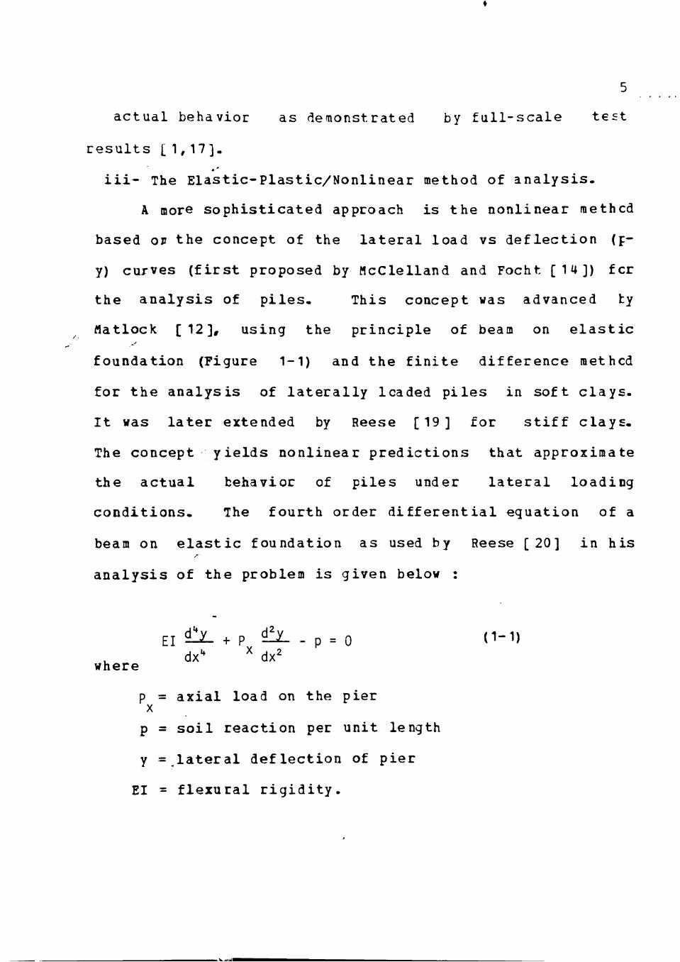
i i i - The E l a s t i c - P l a s t i c / N o n l i n e a r method of a n a l y s i s .
A more s o p h i s t i c a t e d approach i s the nonlinear method
based or the concept of the l a t e r a l load vs d e f l e c t i o n (p-
y) curves ( f i r s t proposed by McClelland and Focht [ 1 4 ] ) fcr
the a n a l y s i s of p i l e s . This concept was advanced ty
Matlock [ 1 2 ] , using the pr inc ip l e of beam on e l a s t i c
foundation (Figure 1-1) and the f i n i t e d i f f erence methcd
for the a n a l y s i s of l a t e r a l l y leaded p i l e s in s o f t c l a y s .
I t was l a t e r extended by Reese [ 1 9 ] for s t i f f c l a y s .
The concept y i e l d s nonlinear p r e d i c t i o n s that approximate
the ac tua l behavior of p i l e s under l a t e r a l loading
c o n d i t i o n s . The fourth order d i f f e r e n t i a l equation of a
beam on e l a s t i c foundation as used by Reese [ 20] in h i s
a n a l y s i s of the problem i s given below :
EI d!iL + p df^ . p = 0 (1-1)
where dx"* ^ dx^
p = a x i a l load on the pier X
p = soil reaction per unit length
y = lateral deflection of pier
EI = flexural rigidity.
Lateral Resistance
77?3 v77=55C
9 I
p .
•> ^
\ I I
. • • •
• «
I
< V
«»,
• V
'>
—AMAA—^
; - ^ V V W - ^
Figure 1-1. Single Lateral Spring Model
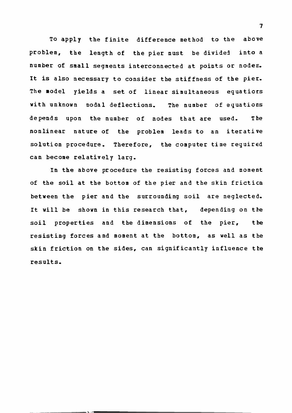
To apply the finite difference method to the above
problem, the length of the pier must be divided into a
number of small segments interconnected at points or nodes.
It is also necessary to consider the stiffness of the pier.
The model yields a set of linear simultaneous eguatiots
with unknown nodal deflections. The number of equations
depends upon the number of nodes that are used. The
nonlinear nature of the problem leads to an iterative
solution procedure. Therefore, the computer time required
can become relatively larg.
In the above procedure the resisting forces and moment
of the soil at the bottom of the pier and the skin fricticn
between the pier and the surrounding soil are neglected.
It will be shown in this research that, depending on the
soil properties and the dimensions of the pier, the
resisting forces and moment at the bottom, as well as the
skin friction on the sides, can significantly influence the
results.
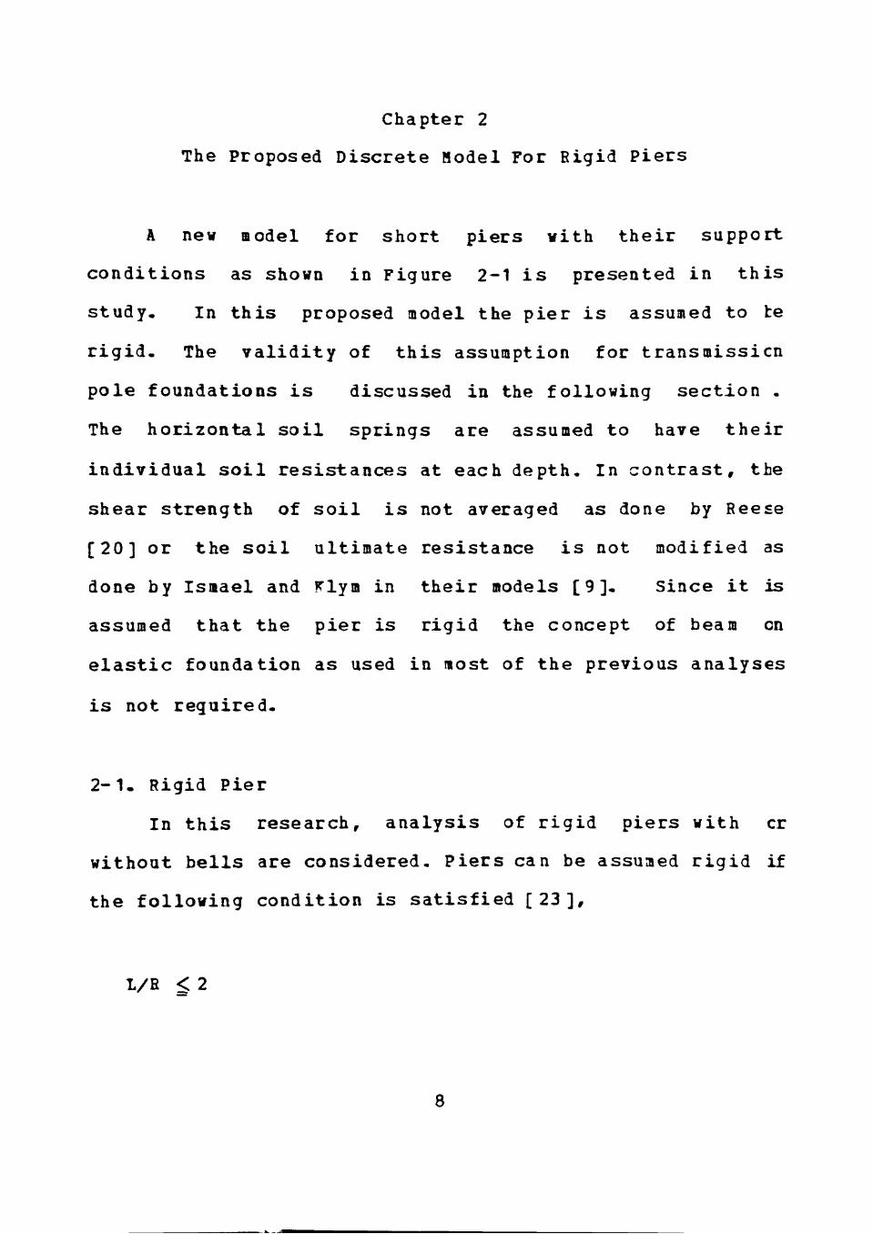
Chapter 2
The Proposed Discrete Model For Rigid Piers
A new model for short piers with their support
conditions as shown in Figure 2-1 is presented in this
study. In this proposed model the pier is assumed to te
rigid. The validity of this assumption for transmission
pole foundations is discussed in the following section .
The horizontal soil springs are assumed to have their
individual soil resistances at each depth. In contrast, the
shear strength of soil is not averaged as done by Reese
[20] or the soil ultimate resistance is not modified as
done by Isaael and jrlym in their models [9]. Since it is
assumed that the pier is rigid the concept of beam on
elastic foundation as used in most of the previous analyses
is not required.
2-1- Rigid Pier
In this research, analysis of rigid piers with cr
without bells are considered. Piers can be assumed rigid if
the following condition is satisfied [23],
I/E < 2
8
Bottom Friction
Bottom Vertical Resistance
Lateral Resistance
Side Fricti on
Bottom Moment
Figure 2-1. The Discrete Multi Spring Model
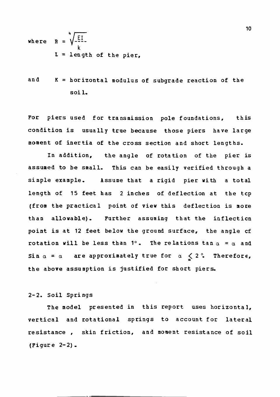
where R k
I = l ength of the p i e r .
10
and K = horizontal modulus of subgrade reaction of the
soil.
For piers used for transmission pole foundations, this
condition is usually true because those piers have large
moment of inertia of the cross section and short lengths.
In addition, the angle of rotation of the pier is
assumed to be small. This can be easily verified through a
simple example. Assume that a rigid pier with a total
length of 15 feet has 2 inches of deflection at the tcp
(from the practical point of view this deflection is more
than allowable). Further assuming that the inflection
point is at 12 feet below the ground surface, the angle cf
rotation will be less than 1°. The relations tana = a and
Sin a = a are approximately true for a < 2 °. Therefore,
the above assumption is justified for short piers.
2-2. Soil Springs
The model presented in this report uses horizontal,
vertical and rotational springs to account for lateral
resistance , skin friction, and moment resistance of soil
(Figure 2-2).
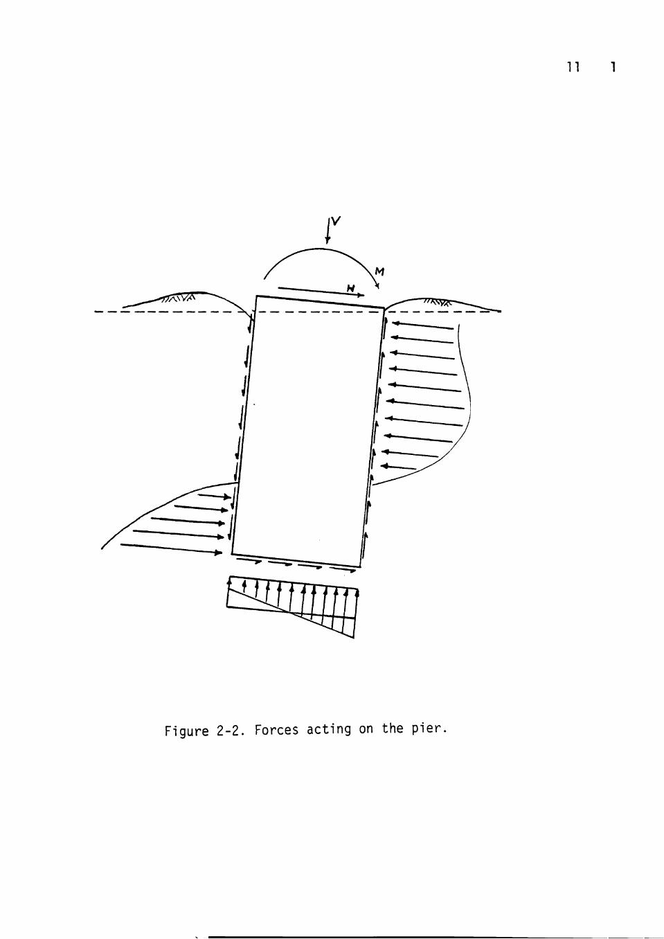
n
Figure 2-2. Forces acting on the pier,
12
Spec i f ic springs, their function and the ir constants
are termed as fol lows : a set of horizontal springs , with
spring constant K , representing the l a t e r a l re s i s tance cf
s o i l . Figure 2-1, , a rotat ional spring, with a spring
constant K. , representing the r e s i s t i n g moment of the
s o i l at the bottom of the pier, a horizontal spring, with a
spring constant K. , representing the fr ic t ion at the
bottom of the p ier , a ver t i ca l spring, with a spring
constant K r representing the vert ica l res istance of s o i l bu
at the bottom of the pier, and a set of vertical springs
representing the skin friction between the pier and the
surrounding soil, with spring constant KJ for the right
side of the pier, and spring constant K for the left side
of the pier.
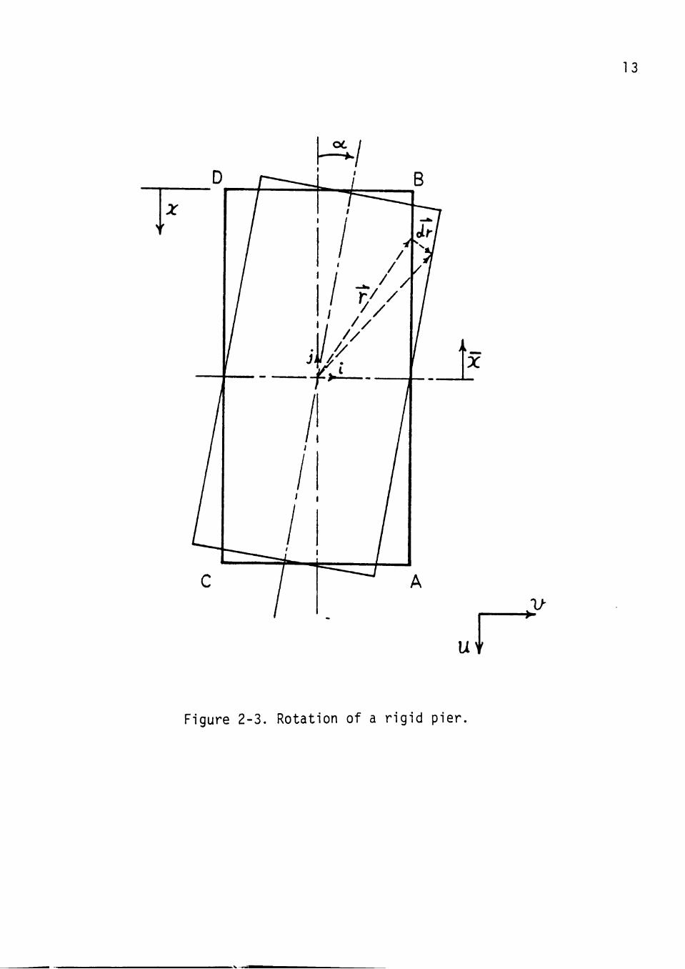
2-3. Development of The System Equations For The Model
To develop the system equations, the geometrical
relationships between the nodal displacements and rigid
body motions of the pier must be established. Assumirg
that the pier experiences a pure rotation. Figure 2-3, the
change in the coordinates of a point on the pier is
determined as follows :
13
V
ul
Figure 2-3. Rotation of a r i g i d p ier .
14
r = R t + X J , 2 . , ^ ,
cir = a X r (2-lb)
"^^ ' ^^ (2-lc)
Where R = radius of the pier
r = p o s i t i o n vector of any node on the pier
a = angle of r o t a t i o n of the p i e r
(c lockwise d i rec t ion)
i , j , k = the c a r t e s i a n unit vectors , a s shown in
Figure 2-3
S u b s t i t u t i n g Equations (2-1a) and (2-1c) i n t o Equation
(2- lb) r e s u l t s in :
dr = - R a j " + y a t (2-2)
using Y = L/2 - X in Equation (2-2) for transformation cf
coordinates
dr = - R a J + (4" - ^ ) ^ " (2-3)
Therefore,
u = R a (2-4) V = (-L. . X) a
where u and v are the vertical and horizontal movements cf
any node along the pier when it has rotated an angle a . If
15
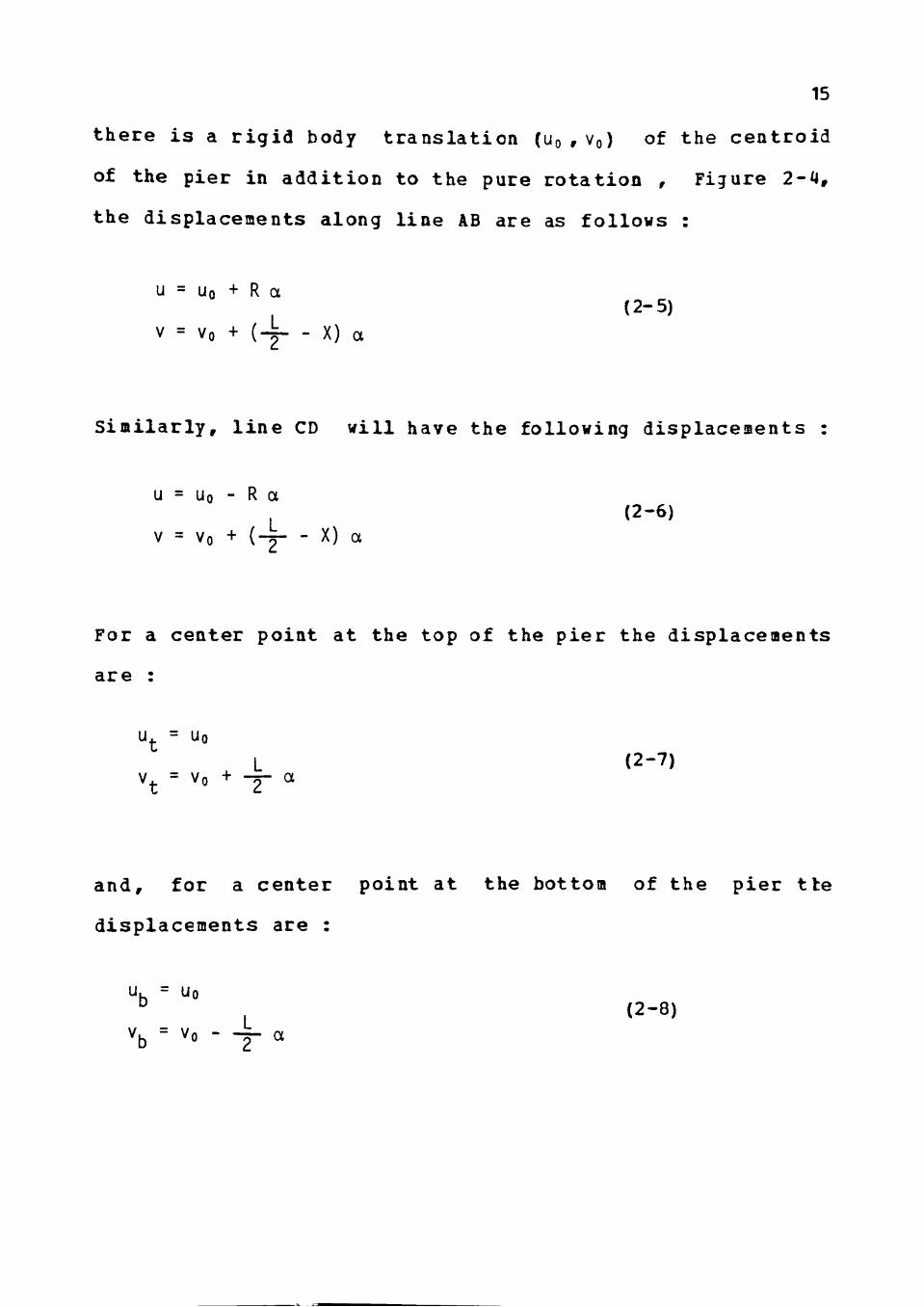
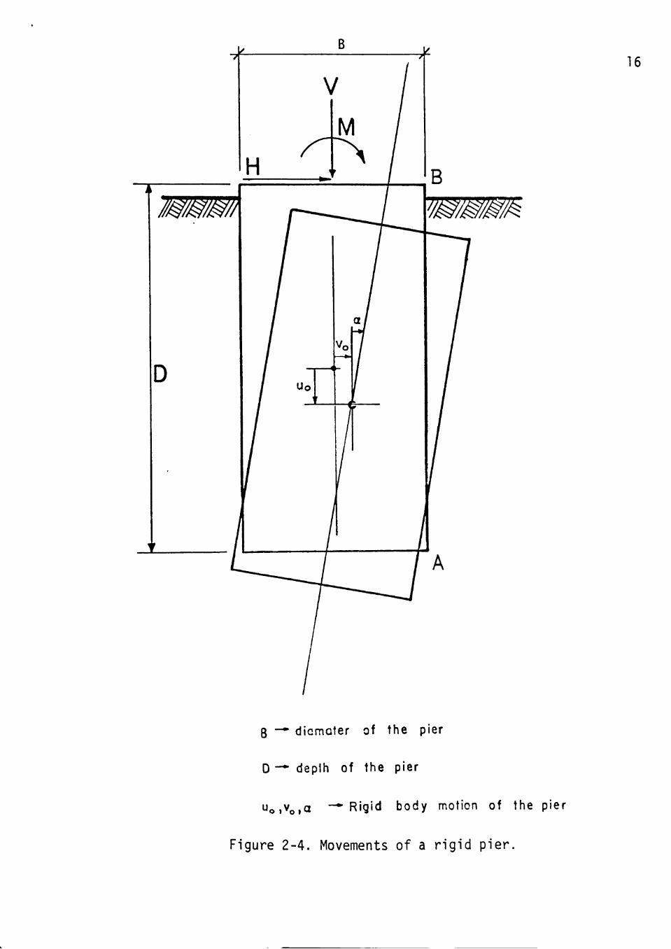
there i s a r i g i d body t r a n s l a t i o n (UQ , VQ) of the c e n t r o i d
of the pier in a d d i t i o n to the pure r o t a t i o n , Figure 2 - 4 ,
the displacements along l i n e AB are as f o l l o w s :
u = Uo + R a (2 -5)
V = Vo + (-— - X) a
S i m i l a r l y , l i n e CD w i l l have the fol lowing displacements
u = Uo - R a (2 -6 )
V = Vo + {-J- - X) a
For a center point at the top of the p i e r the displacements
are :
t = "° L (2-7)
V^ = Vo + - o - ot
and, for a center point at the bottom of the p i er t t e
d i sp lacements are :
U. = Uo
^ (2-8) Vb = Vo - - ^ a
16
B — diamater of the pier
D — deplh of the pier
"o.Vo.a - * Rigid body motion of the pier
Figure 2-4. Movements of a r ig id pier
17
The above equat ions show that i f the r i g i d body
motions of the cen tro id (UQ, VQ) and the angle of r o t a t i o n
a f are known , then the movements of every node on the
p i e r can be determined-
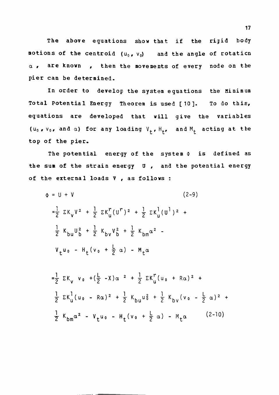
In order to develop the system equat ions the Hinimum
Total P o t e n t i a l Energy Theorem i s used [ 1 0 ] . To do t h i s ,
equat ions are developed that w i l l g i v e the v a r i a b l e s
(Uo,Vor and a) for any loading V. , H., and M. ac t ing a t the
top of the p i e r .
The p o t e n t i a l energy of the system $ i s def ined as
the sum of the s t r a i n energy 0 , and the p o t e n t i a l energy
of the ex terna l loads V , as f o l l o w s :
$ = U + V (2-9)
4 2K^V^ + i Z K ; ; ( U ^ ) ^ + i ZK^(U^)^ +
V^uo - H^(vo + ^ a ) - M^a
=]- ZK^ Vo + ( ^ - X ) a ^ + \ EK[^(UO + Ra)^ +
\ E K J ( U O - R a ) ^ + \ Kj^^u§ + \ K^^(vo - ^ a ) ^ +
\ S m ^ ' - Vt^o - H^(vo ^ ^ a ) - M^a (2 -10)
18
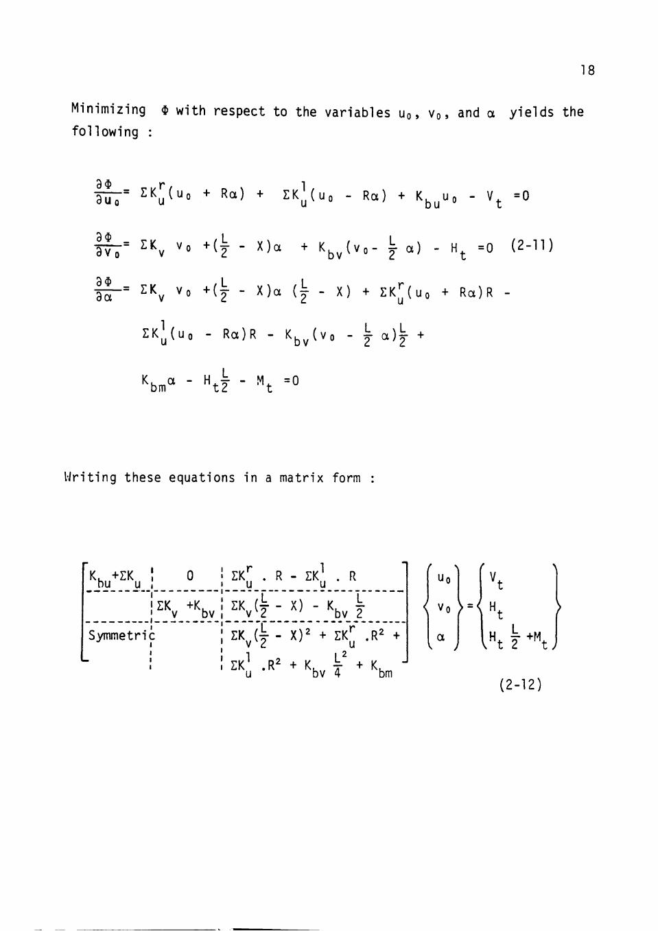
Minimizing $ with respect to the variables UQ, VQ, and a yields the
following :
j ^ - 2:K;J(UO + Ra) + ZK^(uo - Ra) + K ^ ^ U Q - V^ =0
av
9a
•= ZK^ Vo + ( ^ - X)a + K^^(vo- j a) - H^ =0 (2-11)
•= ZK^ Vo +{j - X)a (t . X) + ZK|^(UO + Ra)R -
S K ) (uo - Ra)R - K. (vo - T a)T +
•^Km^ - H.y - M. =0 bm t2 t
Writing these equations in a matrix form :
K. +ZK bu u I
IZK +K. V bv
Symmetric
ZK"^ . R - ZK|J| . R
^ (F- ) -hA ZK^(j - X)^ + ZK[| .R2 +
ZK .R2 + K. X + Kt, u bv 4 bm
r \
< Vo > = <
a V J
V.
H
K\ I '\
(2-12)
19
I t can be concluded from the above analys is that due to the
assumption of a r ig id pier , only three quant i t ies are
required to represent the r ig id body motion of the p ier .
Therefore, the computation time of th i s procedure is
considerably reduced.
As mentioned before, the s o i l spring constants used in
the above s t i f f n e s s matrix vary nonlinearly with the
displacements. The procedures for determining the spring
constants are discussed in chapter 3. In th i s study an
incremental procedure i s used for obtaining the load-
def l ec t ion response of the pier. This procedure is
discussed below.
2 -4 . Procedure for Determining Deflections
The steps involved in solving the nonlinear force-
def lect ion charac ter i s t i c s of a l a t e r a l l y loaded pier are
as fol lows :
Step 1 : The length of the pier i s divided into n
equal segments (generally 10 to 15). Also the load vectcr
i s developed in increments.
Step 2 : A small i n i t i a l value i s assumed for the
angle a equal to 0.0001 radians and the i n i t i a l values cf
UQ and Vo are set to be equal to zero.
20
Step 3 : Using UQ , VQ , and a in equat ions ( 2 - 5 ) , the
v e r t i c a l and hor i zonta l displacements of every node along
the p i e r are c a l c u l a t e d .
u . = Uo + R a
^i = Vo + ( -^ - X) a
Step 4 : Using the s o i l propert i e s ( S , £50. Y ) , the
p-y curves (equations) are developed for each node at i t s
p a r t i c u l a r depth using the procedure in chapter 3 , s e c t i o n
3 - 1 . This s t e p i s executed only once.
Step 5 : The value of v. from s t e p 3 i s s u b s t i t u t e d
i n t o the s tep U equat ions t o obtain the corresponding
f o r c e , and the spr ing constant ( K ) of each s p r i n g .
These values of spring constants w i l l be l a t e r used to
determine the s t i f f n e s s matrix.
Step 6 : The spring c o n s t a n t s , K , found in s t e p 5
t o g e t h e r with the spring cons tant s K^ , K^ , K ^ , and \
determined from the procedure described in chapter 3 cf
t h i s report are s u b s t i t u t e d i n t o Equation ( 2 - 1 2 ) . This
system of equat ions i s then so lved to f ind the new va lues
of Un # Vn # and a -
21
Step 7 : The new values of UQ, VQ , and ^ are
s u b s t i t u t e d in to Equations (2-5) to f ind the new v a l u e s cf
u and v . The d i f f e r e n c e . De l ta , between the new and the
old va lues of v for a point at the top of the p ier i s
determined as f o l l o w s :
Delta = | ( v - V , . ) / v T , I ' * new old ' ^ old '
I f Delta i s l e s s than a prescr ibed to l erance then cont inue
with the next s t e p ; otherwise return to s t ep 3 and
i t e r a t e . The value of the to lerance i s chosen to be 10
in t h i s re search , because t h i s wi l l a l low the system cf
s p r i n g s t o become s u f f i c i e n t l y c l o s e to the s t a t i c
equi l ibr ium from a p r a c t i c a l point of view.
Step 8 : The load vector i s increased by another
increment and the whole process i s repeated. This i s
repeated u n t i l the maximum load i s reached.
Chapter 3
Formulation of Spring Constants
As described in previous chapters, when a tranmissicn
pole i s subjected to la tera l loads (wind or tension cf
cables) i t transfers these loads to i t s pier foundation as
a l a t e r a l load, a ver t i ca l load, and a bending moment.
Therefore, the pier trans lates and rotates in the s o i l as
shown in Figure 2-4. This motion of the pier causes
d i f ferent react ions in the s o i l (Figure 2-2) , including:
l a t e r a l re s i s tance , ver t i ca l res is tanceat at the bo t to i ,
moment at the bottom, f r i c t i on at the bottom, and f r i c t i c n
along the s ides of the pier . The p i e r - s o i l interact ion
c h a r a c t e r i s t i c s due t o these reactions are modeled with
equivalant s o i l spring constants . The development of these
spring constants are discussed below.
3 -1 - The Lateral Spring Constants
The s o i l response to the movements of a l a t e r a l l y
loaded pier i s characterized as a set of discrete springs
s imi lar to the Winkler e l a s t i c foundation concept (1867).
Bat these springs can have nonlinear load-deformaticn
responses , and the response at a point i s independent cf
p ier def lec t ion elsewhere. Obviously t h i s equivalant spring
constant assumption i s not s t r i c t l y valid for s o i l
22
23
continua, but the errors involved in i t s use are assumed to
be small.
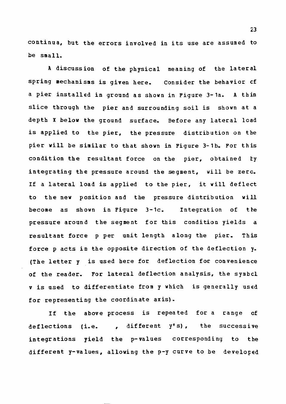
A discussion of the physical meaning of the l a t e r a l
spring mechanisms i s given here. Consider the behavior cf
a pier i n s t a l l e d in ground as shown in Figure 3 - la . A thin
s l i c e through the pier and surrounding s o i l i s shown at a
depth X below the ground surface. Before any l a t era l load
i s applied to the p ier , the pressure dis tr ibut ion on the
pier wi l l be s imilar to that shown in Figure 3 - lb . For t h i s
condit ion the resultant force on the pier , obtained ty
in tegrat ing the pressure around the segment, wi l l be zero.
If a l a t e r a l load i s applied to the p i e r , i t wi l l de f l ec t
to the new pos i t ion and the pressure d is tr ibut ion wi l l
become as shown in Figure 3-1c. Integration of the
pressure around the segment for this condition y i e l d s a
resul tant force p per unit length along the pier . This
force p acts in the opposite direct ion of the def l ec t ion y.
(The l e t t e r y i s used here for def lect ion for convenience
of the reader. For la tera l deflection analys i s , the symbcl
V i s used to d i f f erent ia te from y which i s generally used
for representing the coordinate ax i s ) .
I f the above process i s repeated for a range of
d e f l e c t i o n s ( i . e . , d i f ferent y ' s ) , the success ive
in tegrat ions y ie ld the p-values corresponding to the
d i f ferent y-values , allowing the p-y curve to be developed
24
^ ^
\
V/////.
'/m//^ Ground Surface
A
" \
Xi
View A-A
b- Pressure Distribution
Before Loading
a- Pier Segment
c- Pressure Distribution after Loading
After Reese and Cox (1969)
Figure 3-1. Illustration of Lateral Load Transfer
25
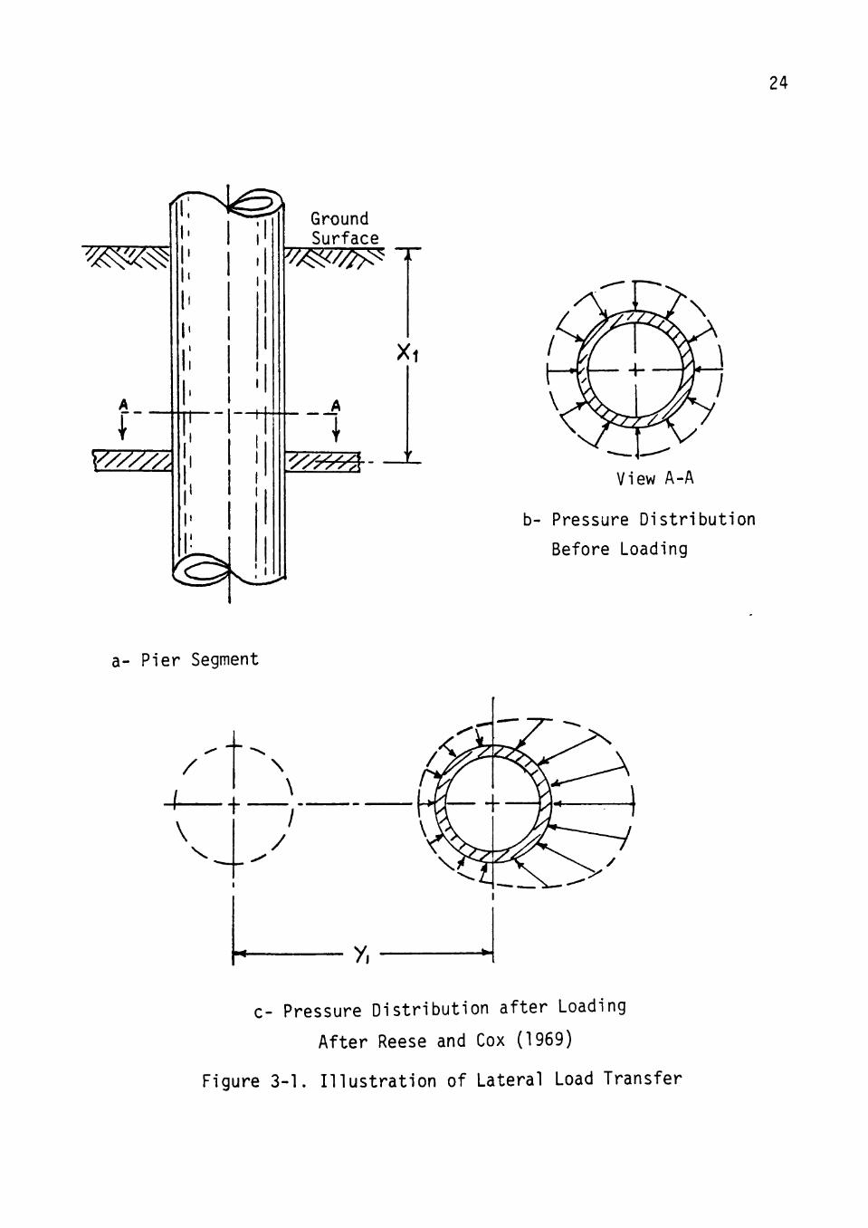
f o r t h e d e p t h X. By a p p l y i n g t h e above p r o c e d u r e t o o t h e r
d e p t h s , a f a m i l y of p-y c u r v e s can be d e v e l o p e d a s in
F i g u r e 3-2a . C u r v e s of F i g u r e 3 -2a r e p r e s e n t t h e
c h a r a c t e r i s t i c s of p-y c u r v e s a t v a r i o u s d e p t h s . The
a b i l i t y t o p r e d i c t t h e b e h a v i o r of p i e r s s u b j e c t e d to
f o r c e s and moments a t t h e t o p i s d i r e c t l y d e p e n d e n t on t h e
a b i l i t y t o d e r i v e t h e p-y c u r v e s g i v i n g t h e s o i l r e s p o n s e
w i th t o l e r a b l e a c c u r a c y .
The d e v e l o p m e n t of P-Y c u r v e s f o r c o h e s i v e s o i l s . As
d e s c r i b e d a b o v e , t h e s o i l r e s p o n s e t o l a t e r a l l o a d s i s
g i v e n by a f a m i l y of c u r v e s g i v i n g s o i l r e s i s t a n c e a s a
f u n c t i o n of p i e r d e f l e c t i o n . The s o i l modul i a r e s e c a n t s to
t h e p - y c u r v e s and can vary i n any a r b i t r a r y manner wi th
d e p t h (and w i t h d e f l e c t i o n of p i e r a s w e l l a s w i t h t h e s o i l
p r o p e r t i e s ) . T h i s i s shown in F i g u r e 3-2b-
A number of i n v e s t i g a t o r s (McCle l land and Foch t [ 1 3 ^ ,
Reese [ 1 8 ] r Mat lock [ 1 2 ] , G i l l and Denars [ 7 ] and R e e s e and
Welch [ 1 9 ] ) have s u g g e s t e d p r o c e d u r e s f o r o b t a i n i n g t h e
r e l a t i o n s h i p be tween t h e s o i l r e a c t i o n p , and p i e r
d e f l e c t i o n y , a t v a r i o u s d e p t h s . The g e n e r a l p r o c e d u r e
f o r o b t a i n i n g a s e t of p-y c u r v e s a t v a r i o u s d e p t h s a l o n g a
p i e r i n c l a y s a s p r o p o s e d by Matlock [ 1 2 ] and R e e s e a rd
Welch [ 1 9 ] i s : T,
26
-»-y
X = X1
Figure 3-2a. Family of p-y curves
X = X2
X = X3
X = X4
Figure 3-2b. Illustration of Secant Modulus
27
1. Determine the variat ions (values) of undrained shear
strength determined from t r i a x i a l compression t e s t s
(CO), e f f e c t i v e unit weight of the s o i l , and £50
the s train corresponding to one-half the maximum
principal s t r e s s di f ference, i . e . ( QI-GS ) max/2,
with depth. In the absence of t r i a x i a l compression
t e s t r e s u l t s , use unconfined compression t e s t
r e s u l t s .
2. Osing the £50 values , compute def lect ion Vso at
one-half the ultimate s o i l reaction by
yso = Ci B £50 ( 3 - 1 )
where
yso = def lec t ion at one-half the ultimate s o i l
react ion;
C, = a constant re lat ing pier def lect ion to the
labratory s tra in ;
B = pier diameter .
3. For a given depth , X , compute the ultimate s o i l
res is tance per unit length of p i e r , P , by
P, = ( 3 + ^ + J - f - ) S^ B 9 S B (3-2)
28
where
S|j = average undrained shear strength of s o i l
from ground surface to depth X;
J = a constant which controls the depth at which
Pu reaches 9cB for cohesive s o i l s ;
B = pier diameter;
Y = average e f f e c t i v e unit weight of s o i l
within the depth X.
U. Compute points describing the p-y curve at depth X
by
^ = 0.5 ( JL )n (3-3)
where
p = s o i l resistance per unit length of p i er ;
y = def lect ion corresponding to p;
n = a constant re lat ing s o i l resistance to pier
de f l ec t ion . 1/n
Note that p = p at y = 2 .yso (3-4)
5. Compute the secant modulus of the s o i l for any value
of y
K = - £ - = ^i! , (3-5) ' ' 2 ySo y'-'
29
Note that i n the computation of the spring
constant K , Eg, (3-5) g ive s i n f i n i t e modulus fcr
y=0 : t h e r e f o r e , in order to prevent the c r e a t i o n cf
such very large spring c o n s t a n t s at small
d e f l e c t i o n s , an a d d i t i o n a l c r i t e r i a i s used here.
For d e f l e c t i o n s l e s s than a d e f l e c t i o n of 0 .5 yso
which corresponds to a s t r a i n equal to 0 .5 £50 in the
s o i l , the spring constant K i s held cons tant at
that p a r t i c u l a r depth. Subs t i tu t ing i n equat icn
(3-5) for y , the i n i t i a l s o i l modulus can te
determined as fo l l ows :
P l/T - ^U
\ - 'TZ^ 7?Pl (3-6) ^ • Yso
Values of the cons tant s C-j , j , and n are based en
empir i ca l c o n s i d e r a t i o n s and t a l l y i n g with a n a l y s i s of load
t e s t r e s u l t s . The proposed va lues of C-j for c l a y s range
from 0.5 (McClelland and Focht [13]) t o 2.5 (Matlock [ 1 2 ]
and Reese and Welch [ 1 9 ] ) . The genera l ly recommended value
of C, =2.0 [ 1 2 , 1 9 ] i s based on Sicempton's e l a s t i c - a n a l y s i s
[ 2 1 ] of a uniformly-loaded area with a l eng th - to -w id th
r a t i o of 10.
For the constant J , va lues in the range of 0.5
(Matlock [12] ) to 2 .83 (Reese [18]) have been sugges ted .
30
The t h e o r e t i c a l e v a l u a t i o n s [ 1 8 ] , load t e s t data [ 1 4 ] , and
b e a r i n g c a p a c i t y t h e o r y [ 2 1 ] i n d i c a t e t h a t the l i m i t i n g
v a l u e of u l t i m a t e l a t e r a l s o i l r e a c t i o n should be o b t a i n e d
a t depths o f about two t o four t imes the p i e r d iameter
c o r r e s p o n d i n g to v a l u e s of parameter J of about 1.5 t o 2 . 8 -
The recommended v a l u e s of exponent n range from 1/3
(Matlock [ 1 2 ] ) t o 1/a (Reese and Welch [ 1 9 ] ) . However, use
of a c t u a l l a b o r a t o r y s t r e s s - s t r a i n c u r v e s , c o r r e s p o n d i n g to
a p p r o x i m a t e l y a v a l u e of n=1/2 , has a l s o been s u g g e s t e d
[ 1 0 ] t o d e f i n e l o a d - d e f l e c t i o n behavior of p i e r s .
A p a r a m e t r i c s tudy was made of the e f f e c t cf
v a r i a t i o n s of C, , J , and n on the computed g r o u n d l i n e
d e f l e c t i o n of a t y p i c a l p i e r ( p i e r # 3 , s e e chapter 4 ) . The
r e s u l t s o f t h i s a n a l y s i s are shown i n F i g u r e ' s ( 3 - 3 to
3 - 5 ) . A s i m i l a r s t u d y was repor ted by Bhushan, Haley , and
Fong [ 2 ] . From t h e t h e o r e t i c a l c o n s i d e r a t i o n s and the
r e s u l t s of t h e above parametr ic s tudy , v a l u e s of C, = 2 . 0 ,
J = 2 . 8 3 , and n=0 .5 were s e l e c t e d f o r computing p-y
c u r v e s .
3-2. The Bottom Vertical Spring Constant
The vertical reaction at the bottom is replaced by a
linear spring placed vertically at the bottom of the pier,
as shown in Fig.2-1.
31
500
400
to Q .
- a
o
ns u
4->
300
200
100
0
-
/ 1
1 1
1 1 / 1 / 1 / /
/ / /
/ /
/ /
/
/ / / /
/ / /
•
y
y y
y y
^y ^
y
**• y
,y
<^
^ ^ -—
1.0 I
,J*^
'7'
^
"^ ' '
-2 .0
0 1 .0 2 .0 3 .0 4 . 0 5 .0
G r o u n d l i n e D e f l e c t i o n ( i n . )
Figure 3-3. Parametric Study (J=2.83, n= l /2 ) .
32
500
400
- 300
-a o
200
03
100
0
.
/ ^ >
II
r
/ /
f /y / y
• ^
y y
y
y y
y y
^ ^ ^
y
y
^ ^ ^ ^
^
- - • ^
^ ^ ^ • * •
^ * ' f
2.ij3
""^T (
1.5
J=0.5
0 1 .0 2 . 0 3 .0 4 .0 5.0
G r o u n d l i n e D e f l e c t i o n ( i n . )
Figure 3-4. Parametric Study (C^=2.0, n= l /2 ) .
33
500
400
to
- 300
• a
o
^ 200 (T3 S-<U
4->
100
0
•
II
yy' < * - •
^ - . - ' • '
^ » ^
•*.
,'^'
\ )
rY=l/4
1/3
0 1 .0 2 .0 3.0 4 .0 5.0
G r o u n d l i n e D e f l e c t i o n ( i n . )
Figure 3-5. Parametric Study (C,=2.0, 0=2.83)
34
the value of the spring constant i s obtained from the
f o l l o w i n g equation for the se t t l ement of a c i r c u l a r f o o t i r g
which i s based on the theory of e l a s t i c i t y [ 3 ]
S = q B ( L I - H ! ) I^ (3.7)
where
S = s e t t l e m e n t , f t
q = i n t e n s i t y of contact pressure, psf
B = l e a s t l a t e r a l dimension of f o o t i n g , f t
y= Poisson's ra t io
E= modulus of e l a s t i c i t y of s o i l , p s f
I = influence factor, equal to 0.88 [31
Therefore, the spring constant of an equivalent spring to
replace t h i s s o i l reaction i s
'''" '- B (1 - ,n I„ '^-^'
3 - 3 . The Bottom Moment Spring Constant
When a l a t e r a l force or a moment i s applied on the top
of a r ig id p i er , the pier tends to ro ta te , and a r e s i s t i r g
moment i s developed at the bottom of the pier, as shown in
Figure 2-2. This react ion of the s o i l at the bottom is
replaced by the rotat ional spring shown in Figure 2 -1 . The
35
spr ing constant i s determined from the fo l lowing equat icn
which was developed by Lee £3 ] for the rotat ion of r i g i d
f o o t i n g s subjected t o a moment M ;
Tan a = J ^ -Lu^ I B3 r m T3 — : % <3-9)
where
a =rotation of footing (radians)
I =shape factor, equal to 6.0 [3]
Note that for small a , tan a = a
Hence
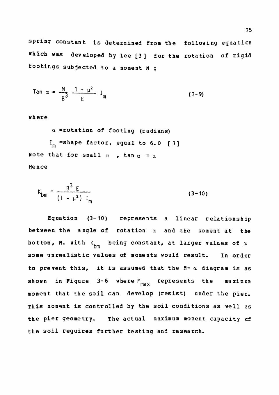
Equation (3-10) represents a linear relationship
between the angle of rotation a and the moment at the
bottom, n. With K. being constant, at larger values of a bm
some u n r e a l i s t i c v a l u e s of moments would r e s u l t . In order
to prevent t h i s , i t i s assumed that the M- a diagram i s as
shown in Figure 3-6 where M represents the maximum ^ max
moment that the soil can develop (resist) under the pier.
This moment is controlled by the soil conditions as well as
the pier geometry. The actual maximum moment capacity cf
the soil requires further testing and research.
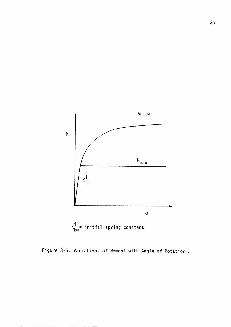
36
M
Actual
a
bm initial spring constant
Figure 3-6. Variations of Moment with Angle of Rotation .
37
In the absence of data on this subject it is assumed
that the maximum allowable stress between the bottom cf
pier and the soil is a function of the shear strength cf
soil S and the vertical stress due to the total vertical
load at the bottom of the pier, P/A , thus:
^ = - -f (3-11)
M max
or "max = S(S^^-£-) ,3.,2,
where
S = sec t ion modulus of the pier cross sect ion
equal to -^—
P = t o t a l v e r t i c a l force at the bottom of the
pier which includes the weight of the pier
L = t o t a l length of the pier
Equation (3-12) s impl i f i e s to the following
M = 4 - ^ ( s + - ^ ) (3-13) max 32 ' u A
The M obtained above i s very conservative because of the max "*
38
s i m p l i f i c a t i o n t h a t i s made t o the M-° diagram (Figure
2 - 9 ) . By knowing the maximum moment t h a t t h e s o i l can
t o l e r a t e and the i n i t i a l v a l u e of \m ' ^^^ M-a
r e l a t i o n s h i p i s deve loped- Then by knowing t h e v a l u e cf
t h e r o t a t i o n a f o r each l oad ing c o n d i t i o n , the
c o r r e s p o n d i n g va lue of K, can be determined . To accompl i sh bm
this, an initial value of K. is determined first and then
the moment M is calculated as ^ = 'bm ° • ^^^' ^^ ^^^
new calculated moment is more than \g^x ' ^ ® secant spring
constant is calculated by the following equation :
M K = ^^^ (3-14) bm a
3-4- The Bottom Frict ion Spring Constant
The behavior due to the fr ic t ion at the bottom is
represented by a horizontal spring at the bottom (Figure
2 - 1 ) . In the absence of experimental data, the
re la t ionsh ip between the f r i c t i o n a l force and the l a t e r a l
movement of the bottom of pier i s assumed as shown in
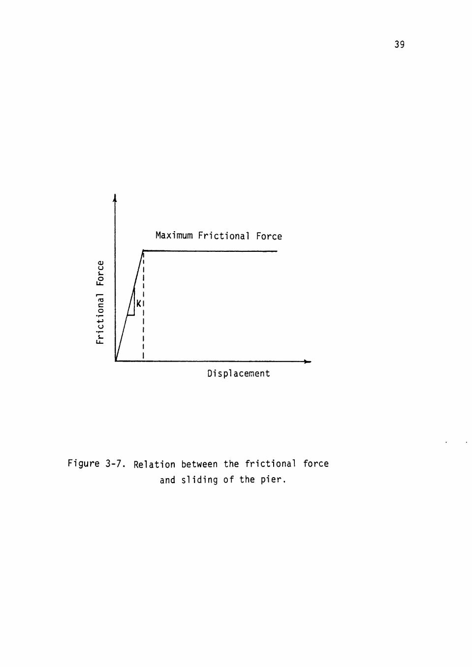
Figure 3-7. The f r i c t i o n a l force w i l l reach a constant
maximum value after a prescribed displacement. I t i s
further assumed that the value of the prescribed
dislplacement i s about 0.01 f t . This assumption i s based on
experiments conducted by other inves t igators [ 2 2 ] .
39
u i-o
C
o •r-
o
Maximum Frictional Force
Displacement
Figure 3-7. Relation between the frictional force
and sliding of the pier.
The maximum frictional stress at the bottom is given
by:
a = Sj + -^ Tan 4) (3-15)
where S = shear s trength of s o i l
P = load a t the bottom of the p ier
A = area at the bottom (be l l )
L = length of the pier
Therefore , the maximum f r i c t i o n a l force w i l l be
F = (S + 4 - Tan (J) ) A (3-16) rmax ^ u A
Hence, i n i t i a l l y ,
>/i ^rmax. (3-17) • bv " 0.01
where i t i s assumed that the F ^ ^ i s reached when t t e
d i f f e r e n t i a l displacement between the p ier and the s o i l i s
0.01 f t .
I f the displacement at the bottom of the p ier i s found
to be more than 0.01 f t . then the new spring constant w i l l
be a secant modulus determined from the f o l l o w i n g
r e l a t i o n :
F K = rmax (3-18) bv V
41
where v i s the l a t e r a l d e f l e c t i o n of the bottom of the
p i e r .
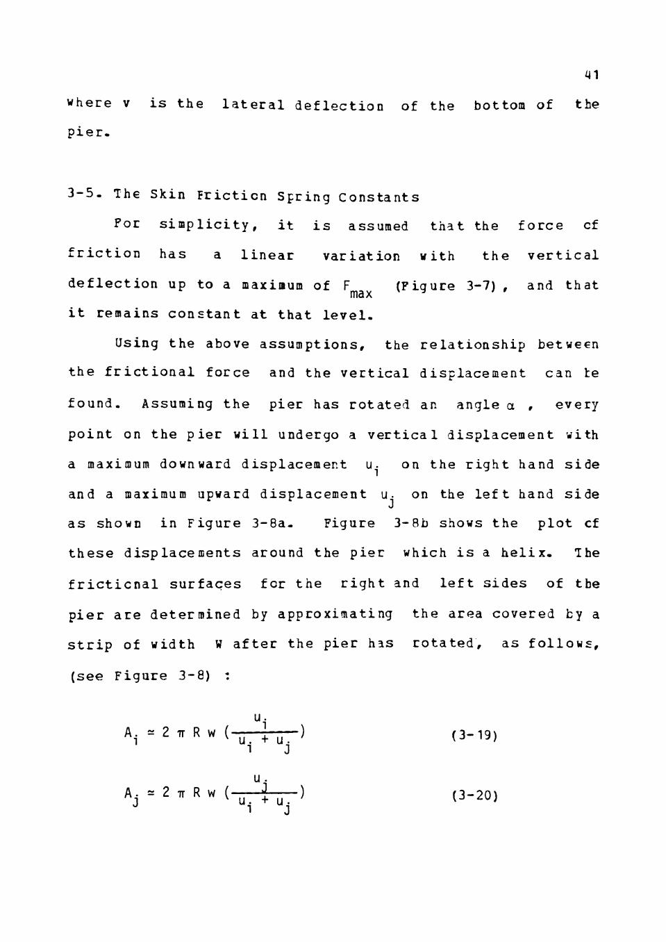
3 - 5 . The Skin F r i c t i c n Spring Constants
For s i m p l i c i t y , i t i s assumed that the force cf
f r i c t i o n has a l i n e a r var iat ion with the v e r t i c a l
d e f l e c t i o n up to a maximum of F (Figure 3-7) , and that max ^ ^ ' '
it remains constant at that level.
Using the above assumptions, the relationship between
the frictional force and the vertical displacement can te
found. Assuming the pier has rotated an angle a , every
point on the pier will undergo a vertical displacement with
a maximum downward displacement u. on the right hand side
and a maximum upward displacement u- on the left hand side
as shown in Figure 3-8a- Figure 3-8b shows the plot cf
these displacements around the pier which is a helix. The
frictional surfaces for the right and left sides of the
pier are determined by approximating the area covered by a
strip of width W after the pier has rotated, as follows,
(see Figure 3-8) :
i i " 2 TT R w ( .H ,. ) (3-19)
u.
^ " " u. i u. ' t3-20)
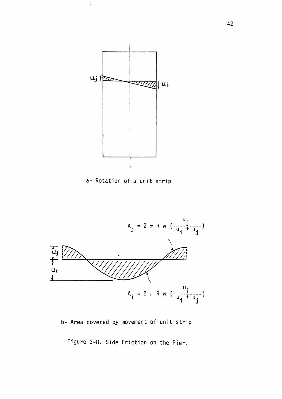
42
Ui 4^77>>.^ 1 -^^^.iV^ luc
a- Rotation of a unit strip
u. A.. = 2 , R w (--"i--")
u. A. ^ 2 TT R w ( 1 - — )
u. + u. ' 1 J
b- Area covered by movement of unit strip
Figure 3-8. Side Friction on the Pier.
43
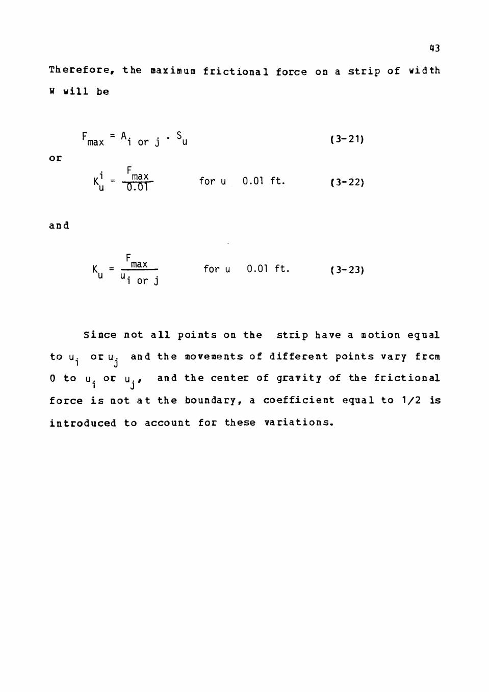
T h e r e f o r e , t h e maximum f r i c t i o n a l f o r c e on a s t r i p of width
W w i l l be
or
and
F = A. . . S. max 1 or J u
(3-21)
F K. = -TTTTr ^Or ^ 0-01 f t - (3-22) u inrr
F K = "^^^ fo r u 0.01 f t . (3-23) ^ ^ i or j
Since not a l l points on the s tr ip have a motion equal
to u. o r u . and the movements of dif ferent points vary frcra
0 to u. or u.# and the center of gravity of the f r i c t i o n a l
force i s not at the boundary, a coe f f i c i ent equal to 1/2 i s
introduced to account for these variat ions .
Chapter 4
Behavior Of The Model
TO assess the behavior of the a n a l y t i c a l model, t*io
types of study a re conducted, (1) s tudy of inf luence cf
va r ious s o i l sp r ings on load -de f l ec t ion response foe a
t y p i c a l p i e r , and (2) comparison of the a n a l y t i c a l l y
obta ined l o a d - d e f l e c t i o n responses with f i e ld t e s t data fcr
seven d i f f e r e n t p i e r s . These s t u d i e s a re presented below.
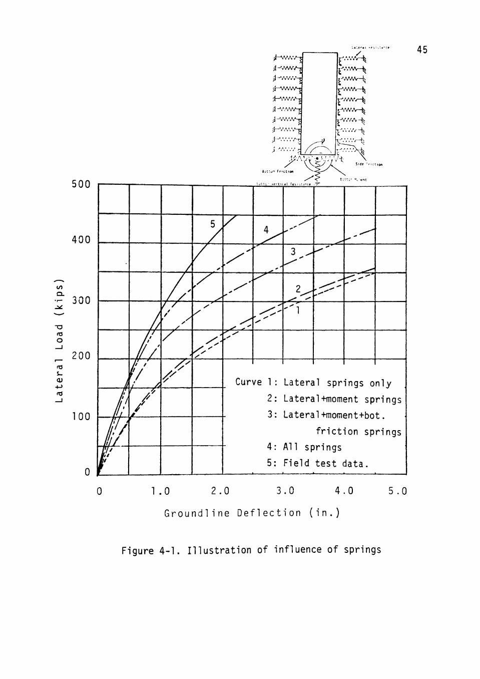
4 - 1 . Inf luence Of Soi l Springs
As discussed prev ious ly in chapter 2 (Ref. Figure
2 - 1 ) , the a n a l y t i c a l model incorpora tes s o i l sp r ings for
s i d e f r i c t i o n , bottom f r i c t i o n , bottom v e r t i c a l r e s i s t a n c e ,
and bottom moment i n addi t ion to the l a t e r a l r e s i s t a n c e
s p r i n g s . To assess the inf luence of these var ious s o i l
s p r i n g s , a p i e r of dimensions 4 f t . diameter and 15 f t .
long for which f i e ld t e s t data are a v a i l a b l e i s analyzed to
ob ta in l o a d - d e f l e c t i o n response. s o i l p r o p e r t i e s ard
r e l a t e d p i e r data are given in Example 1 in the next
s e c t i o n . The l oad -de f l ec t i on response for t h i s p i e r i s
f i r s t determined using only the l a t e r a l s o i l sp r ings (curve
1, Figure 4 - 1 ) . Then other spr ings are added one a t a t i n e
to t h i s t y p i c a l p i e r model and the corresponding load-
d e f l e c t i o n responses a re determined.
44
LA'.er^ I - f . : •. l^-CP
500
400
to
- 300
-a
o
200 03 S-
100
0
45
Curve 1 : Lateral springs only
2: Lateral+moment springs
3: Lateral+moment+bot.
friction springs
4: All springs
5: Field test data.
0 1 .0 2.0 3.0 4.0 5.0
Ground l ine D e f l e c t i o n ( i n . )
Figure 4 -1 . I l lus t ra t ion of influence of springs
46
In t h i s particular example the e f f e c t of the bottom
r e s i s t i n g moment (curve 2) , Figure 4-1 , on reducicg
de f l ec t i ons i s not very s igni f icant due to the small
diameter of the b e l l . This feature can become more
e f f e c t i v e for a pier with a larger b e l l , or i f the s o i l
strength at the bottom i s much higher than at the top. The
addit ion of the bottom f r i c t i o n spring (curve 3), Figure
4 - 1 , and also the s ide f r i c t i on springs (curve 4 ) , Figure
4 - 1 , seem to have s ign i f i cant e f f ec t s on reducing the pier
d e f l e c t i o n s . As a resu l t of a l l the features that have been
added, the f i n a l r e s u l t s are reasonably c lose to the f i e ld
t e s t data up to a load of about 250 kips (Ref. Figure 4-1) .
4 -2 . Comparison Of Bodel Results With Field Test Data
Bhushan, Haley, and Fong [ 2 ] have reported f i e l d t e s t
data on twelve pier foundations. Of these , s ix piers were
on sloping ground or they were r e l a t i v e l y f l ex ib le p iers .
The remaining s ix piers could be c l a s s i f i e d as r ig id piers
(L/R varies from 1.5 to 1 .9) . These s i x piers are used fcr
the comparison of model r e s u l t s with f i e l d t e s t data. An
addit ional pier foundation was chosen from a f i e l d t e s t
reported by Ismael and Klym [ 9 ] . This could a l so te
regarded as a r ig id pier (L/R=1.3).
47
The actual properties of the soil as presented ty
Bhushan, Haley, and Fong [2] are reproduced in Tables 4-1
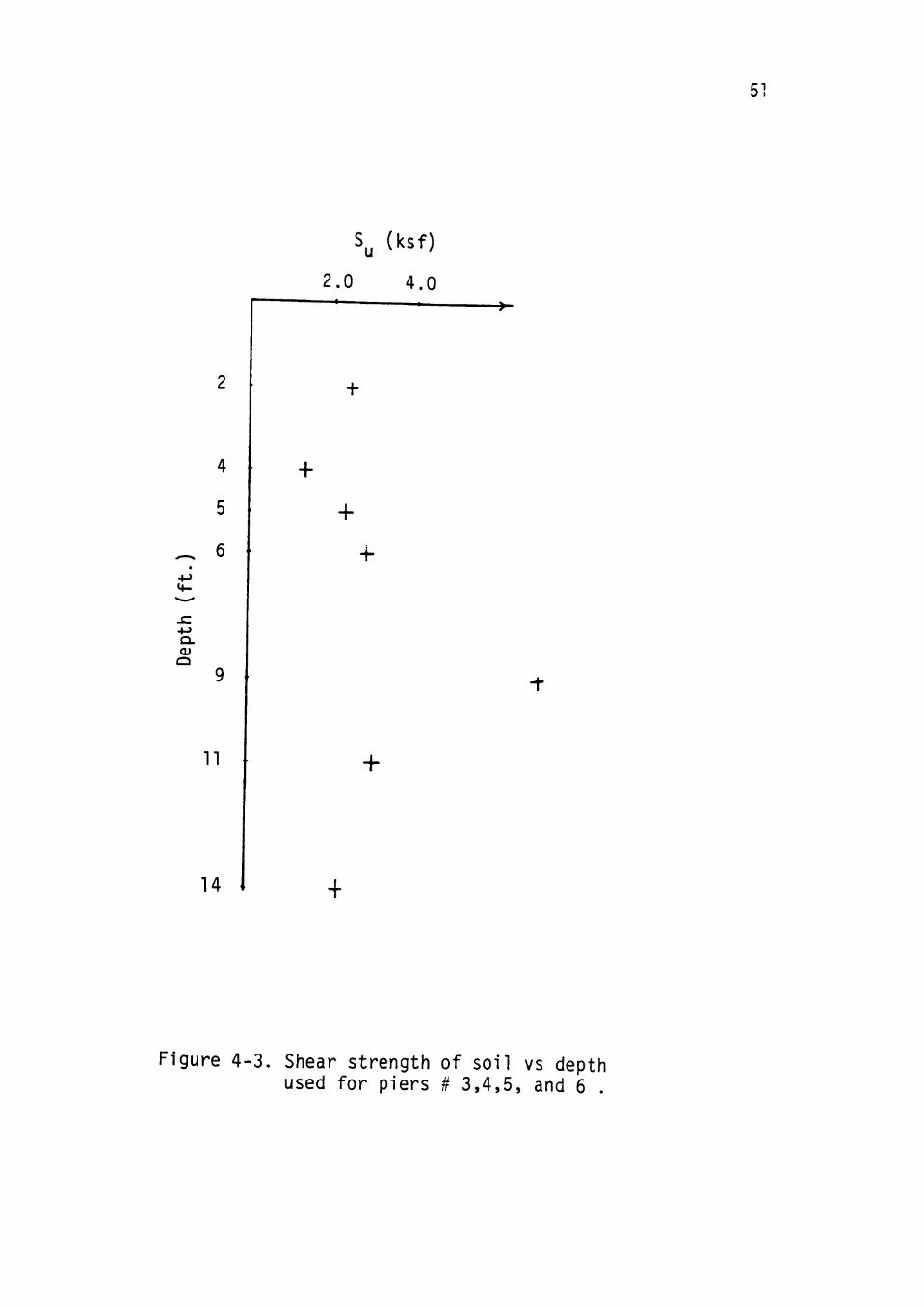
and 4-2 for convenience. Figure 4-2 and 4-3 (data fcr
ploting these Figures are obtained from Tables 4-1 and 4-2)
are also presented here as a convenient way fcr
interpolating the shear strength of soil for the depths at
which the soil data are not given in Tables 4-1 and 4-2.
In the absence of the value of cohesion and angle cf
internal friction of the soil, the Standard Penetration
Test results are used to predict the average strength
parameters. In order to relate the SPT blow counts N, to
the shear strength of soil an approximate equation c = N/8
ksf is used [ 4 ].
Results of analysis using the model are compared with
field test data for following seven piers. In each case
pier dimensions and soil properties are given, and lateral
load-deflection results are compared.
48
Table 4 - 1 . S o i l P r o p e r t i e s for P i e r s * 1 and 2
Depth
f t .
2
4
6
9
11
14
SPT^
N
19
34
—
-
35
44
20
20
0.'
ksf
-
0 . 7 2
1 . 4 4
2 . 8 8
—
0
-
0
cu s
uu
ksf
—
10.8
11.2
12.3
>
8.8
-
3.6
a c
ksf
3,8 17°
a £^50
%
—
0 . 7
0 . 9
1 .0
-
1 . 7
—
0 . 8
used
S u
ksf
2 . 4
4 . 0
4 . 4
4 . 4
2 . 5
1 .8
used
%
0 . 9 4
0 . 9 4
0 . 9 4
0 . 9 4 1
0 . 9 4
0 . 9 4
a. From t e s t s by Bhushan, Haley, and Fong [ 2 ]
^9
Table 4 - 2 . S o i l P r o p e r t i e s for P i e r s # 3 , 4 , 5 , and 6
D e p t h
f t .
2
4
5
6
9
11
14
SPT^
N
19
30
-
—
32
22
43
24
31 r 1 _
—
—
a 03
k s f
—
0 . 7 2
1 .44
2 . 8 8
0
-
0
-
0
0 . 7 2
1 .44
2 . 8 8
CO 5^
00
k s f
-
6 . 6
9 . 6 J>
14 .6
4 . 6
-
1 4 . 0
-
3 .9 \
7 . 7
1 1 . 8 >
c^
k s f
0.9
1.0
* ^
1
41°
35°
a £ 5 0
%
—
0 -6
0 . 8
0 . 8
0 . 7 6
-
—
-
—
0 .6
0 . 7
1 . 1
used
S
k s f
2 . 4
1.3
2 . 3
2 . 8
7 . 0
3 . 0
2 . 2
u s e d
£ 5 0
^
0 . 7 2
0 . 7 2
0 . 7 2
0 . 7 2
0 . 7 2
0 . 7 2
0 . 7 2
a . From t e s t s by Bhushan, Haley, and Fong [ 2 ]
50
2.0
S, (ksf)
4.0
^ 6
+
+
4-> Q. CU O
+
+
11
14
+
+
Figure 4-2. Shear strength of soil vs depth used for piers # 1 and 2.
51
4
5
6
Q.
O
11
14 I
2.0
\ (ksf)
4.0
+
+ -h
+
+
•f
Figure 4-3. Shear strength of soil vs depth used for piers # 3,4,5, and 6 .
52
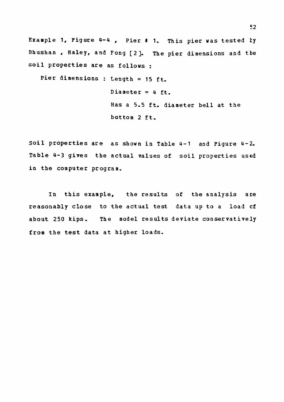
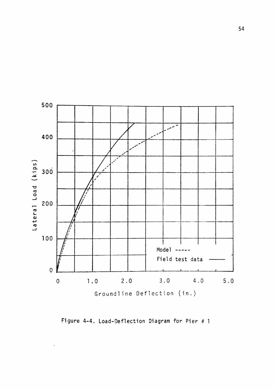
Example 1, F i g u r e 4-4 , P i e r # 1. This p i e r was t e s t e d ty
Bhushan , Ha ley , and Fong [ 2 ] . The p i e r dimensions and the
s o i l p r o p e r t i e s are as f o l l o w s :
P i e r d i m e n s i o n s : Length = 15 f t .
Diameter = 4 f t .
Has a 5 .5 f t . d iameter b e l l at t h e
bottom 2 f t .
S o i l p r o p e r t i e s are a s shown i n Table 4 -1 and Figure 4 - 2 .
Tab le 4-3 g i v e s t h e a c t u a l v a l u e s of s o i l p r o p e r t i e s used
i n t h e computer program.
In t h i s example , t h e r e s u l t s of the a n a l y s i s are
r e a s o n a b l y c l o s e to t h e a c t u a l t e s t data up t o a l oad cf
about 250 k i p s . The model r e s u l t s d e v i a t e c o n s e r v a t i v e l y
from t h e t e s t data a t h igher l o a d s .
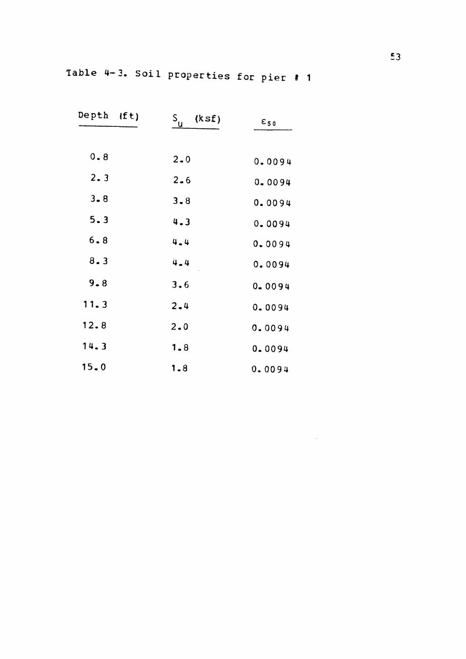
Table 4-3. Soil properties for pier # 1
53
D e p t h
0 . 8
2 . 3
3 . 8
5 . 3
6 . 8
8 . 3
9 . 8
1 1 . 3
1 2 . 8
1 4 . 3
1 5 . 0
<ft) S^ (ks f )
2 . 0
2 . 6
3 . 8
4 . 3
4 . 4
4 . 4
3 . 6
2 . 4
2 . 0
1.8
1.8
^ 5 0
0 . 0 0 9 4
0 . 0094
0 . 0094
0. 0094
0 . 0094
0. 0094
0. 0094
0. 0094
0 . 0094
0 . 0 0 9 4
0 . 0094
54
500
400
to
- 30() .1^
O
200 <0
TOO
0
•
i
h fi 11
II ii
It ji ii
II
II ji II
If
i 1 11
11
/ /
/ /
/ X / y / /
/ f
•
0
y 0
•
Mo
^ . ' ^
^
del — F i p l ^ ^a.e-¥ ^ a ^ r 1 C 1 VJ 1<C
0 1 .0 2.0 3.0 4.0 5.0
Groundline Deflection (in.)
Figure 4-4. Load-Deflection Diagram for Pier # 1
55
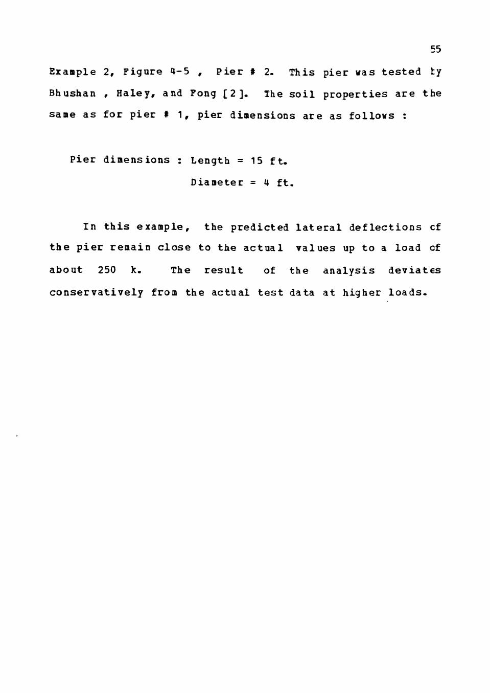
Example 2, Figure 4-5 , P i e r # 2- This pier was t e s t e d ty
Bhushan , Haley, and Fong [ 2 ] . The s o i l propert ies are the
same as for p ier # 1 , pier dimensions are as fo l l ows :
Pier dimensions : Length = 15 f t .
Diameter = 4 ft ,
In t h i s example, the predicted l a t e r a l d e f l e c t i o n s cf
the p i e r remain c l o s e to the ac tua l va lues up to a load cf
about 250 k. The r e s u l t of the a n a l y s i s d e v i a t e s
c o n s e r v a t i v e l y from the actual t e s t data at higher l o a d s .
'>r ::-,_ Ai--:^ry? .•
55
;; uu
400
- 300
• o f8 O
200
tera
l
1
100
0
-
/ / /
/ / / /
/ / r
11 If 11
/ / / /
/ / / / / /
7 1
y
/ ^
> y'
y
1
/ y
y y
Mo
Fi 1
y y
del --'
eld te'^''' ' ^^ 1 1 <
1,0 2.0 3.0 4.0 5.0
Groundline Deflection (in.)
Figure 4-5. Load-Deflection Diagram for Pier # 2
r i
57
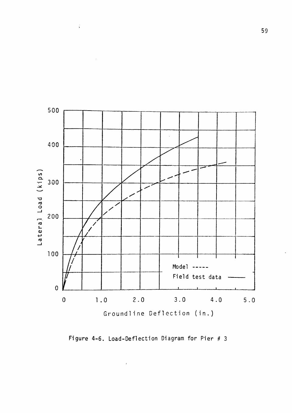
Example 3, Figure 4-6 , P i er # 3. This p ier was t e s t e d ty
Bhushan , Haley, and Fong [ 2 ] . The pier dimensions and the
s o i l p r o p e r t i e s are as fo l l ows :
P ier dimensions : Length = 12.5 f t .
Diameter = 4 f t .
Has a 5.5 f t . diameter b e l l at the
bottom 2 f t .
S o i l p r o p e r t i e s are a s shown in Table 4-2 and Figure 4 -3 .
Table 4-4 g i v e s the ac tua l values of s o i l proper t i e s used
in the computer program.
In t h i s example the r e s u l t of the a n a l y s i s i s c l o s e to
the a c t u a l t e s t data up to an ul t imate load of about 200 k.
However, they d e v i a t e conserva t ive ly from the actua l t e s t
data a t higher l o a d s .

Table 4-4. Soil properties for pier # 3
58
D e p t h
0 . 6
1.9
3 . 1
4 . 4
5 . 6
6 . 9
8 . 1
9 . 4
1 0 . 6
1 1 . 9
1 2 . 5
( f t ) S u
2 . 0
2 . 4
1.9
1.8
2 . 6
4 . 0
6 . 0
6 . 0
3 .5
2 . 7
2 . 7
i^-s f ) £ 5 0
0 . 0 0 7 2
0. 0072
0 . 0 0 7 2
0 . 0 0 7 2
0 . 0 0 7 2
0 . 0 0 7 2
0 . 0 0 7 2
0. 0072
0 . 0 0 7 2
0 . 0 0 7 2
0 . 0 0 7 2
59
500
400
to
- 300
-a o
200 rt3 s .
(T3
100
0
0 1.0 2 . 0 3 .0 4 .0 5 .0
Groundline Deflection (in.)
Figure 4-6. Load-Deflection Diagram for Pier # 3
60
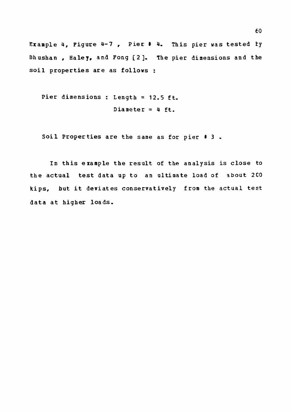
Example 4, Figure 4-7 , P i e r » 4. This pier was t e s t e d ty
Bhushan , Haley, and Fong [ 2 ] . The pier dimensions and the
s o i l p r o p e r t i e s are as fo l l ows :
Pier dimensions : Length = 12.5 ft.
Diameter = 4 ft.
S o i l Properties are the same as for pier # 3 .
In t h i s example the resul t of the analysis i s c l o s e to
the actual t e s t data up to an ultimate load of about 2C0
k ips , but i t deviates conservatively from the actual t e s t
data at higher loads .
61
500
400
to Q.
o
+-> (T3
300
200
100
0 L 0 1.0 2.0 3.0 4.0 5.0
Groundline Deflection (in.)
Figure 4-7. Load-Deflection Diagram for Pier # 4
62
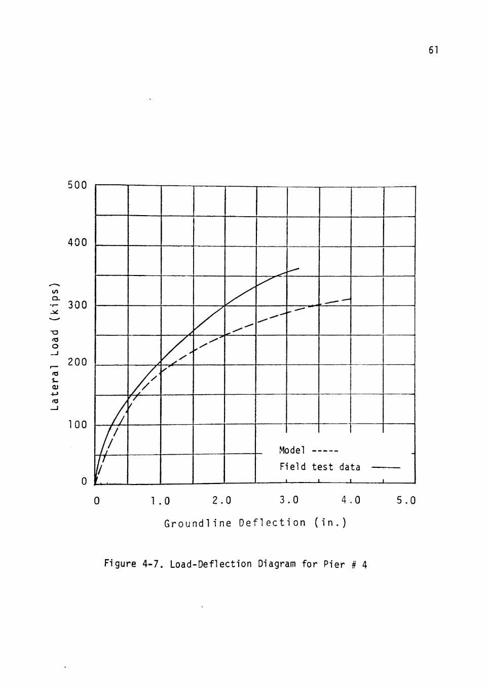
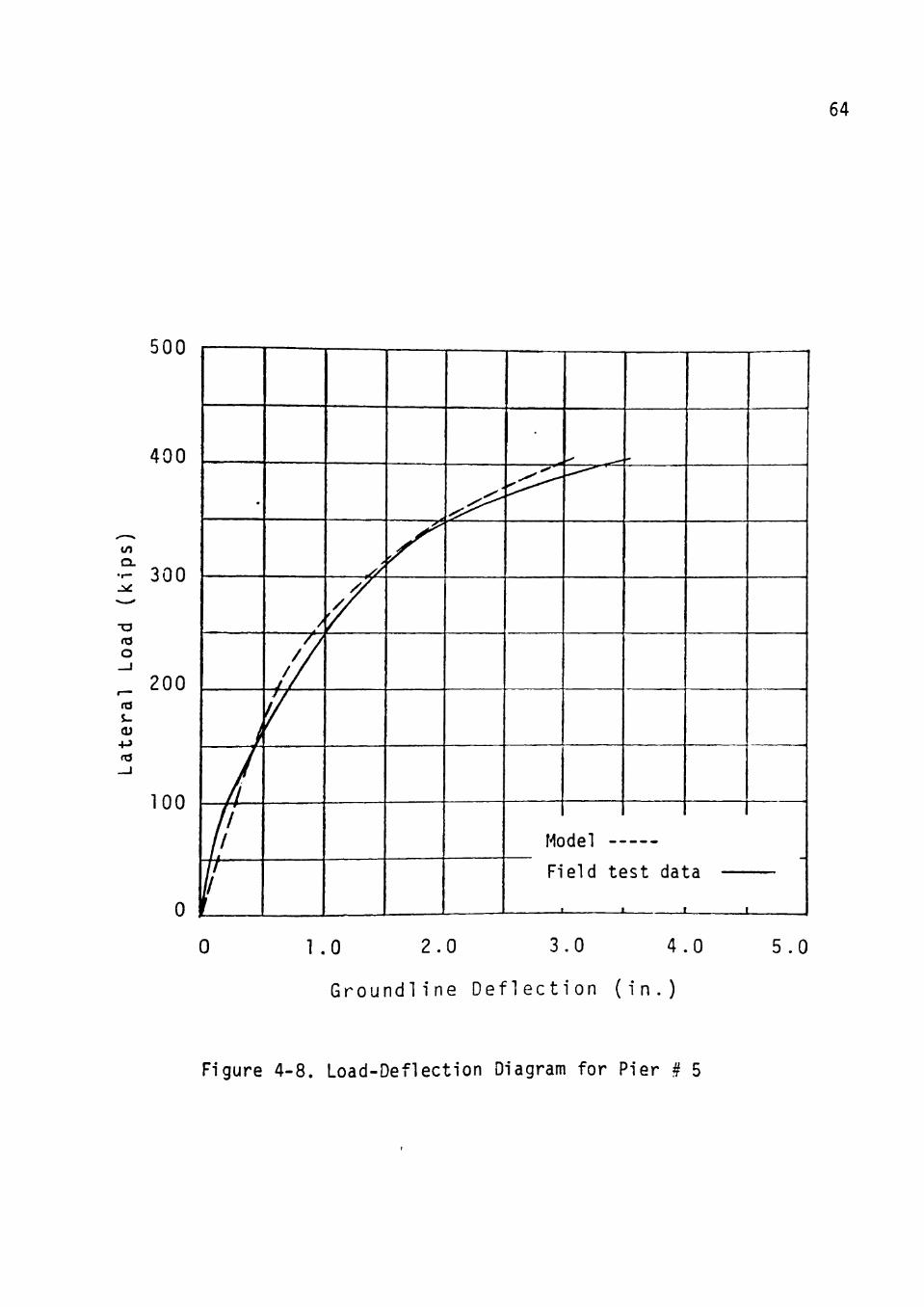
Example 5, Figure 4-8 , Pier # 5. This pier was tested ty
Bhushan r Haley, and Fong [2]. The pier dimensions and the
soil properties are as follows :
Pier dimensions : Length = 15.5 ft
Diameter = 4 ft.
Has a 5.5 ft. diameter bell at the
bottom 2 ft.
Soil properties are as shown in Table 4-2 and Figure 4-3.
Table 4-5 gives the actual values of soil properties used
in the computer program-
In this example the result of the analysis is very
close to the actual test data up to the maximum load of
400 k.
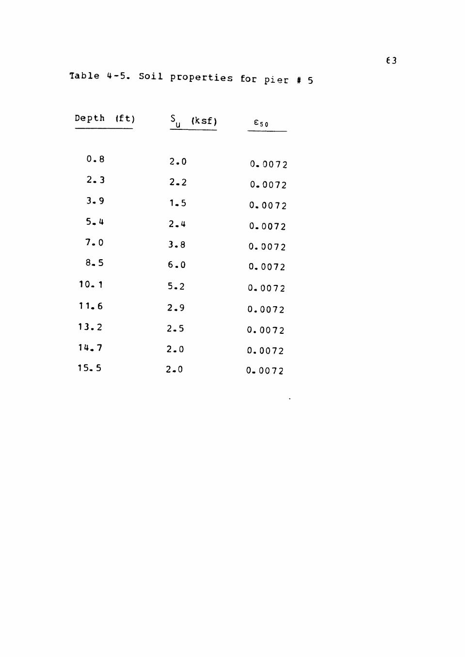
Table 4-5. Soil properties for pier # 5
€3
Depth
0.8
2.3
3.9
5.4
7.0
8.5
10. 1
11.6
13.2
14.7
15.5
(ft) S u
2.0
2.2
1.5
2.4
3.8
6.0
5.2
2.9
2.5
2.0
2.0
(ksf) ^50
0. 0072
0.0072
0.0072
0.0072
0. 0072
0. 0072
0. 0072
0.0072
0. 0072
0.0072
0. 0072
64
500
400
to
- 300
o
200
i.
«T3
100
0
•
/
/ /
/ /
/ /
^ //
/ / / /
/ / / /
^
/ / / /
'/
.,yy^
"^ 7 5 ^
- — — — -
1
Model
Field test data
— 1 _ _ J. I 1
0 1.0 2.0 3.0 4.0 5.0
Groundline Deflection (in.)
Figure 4-8. Load-Deflection Diagram for Pier # 5
65
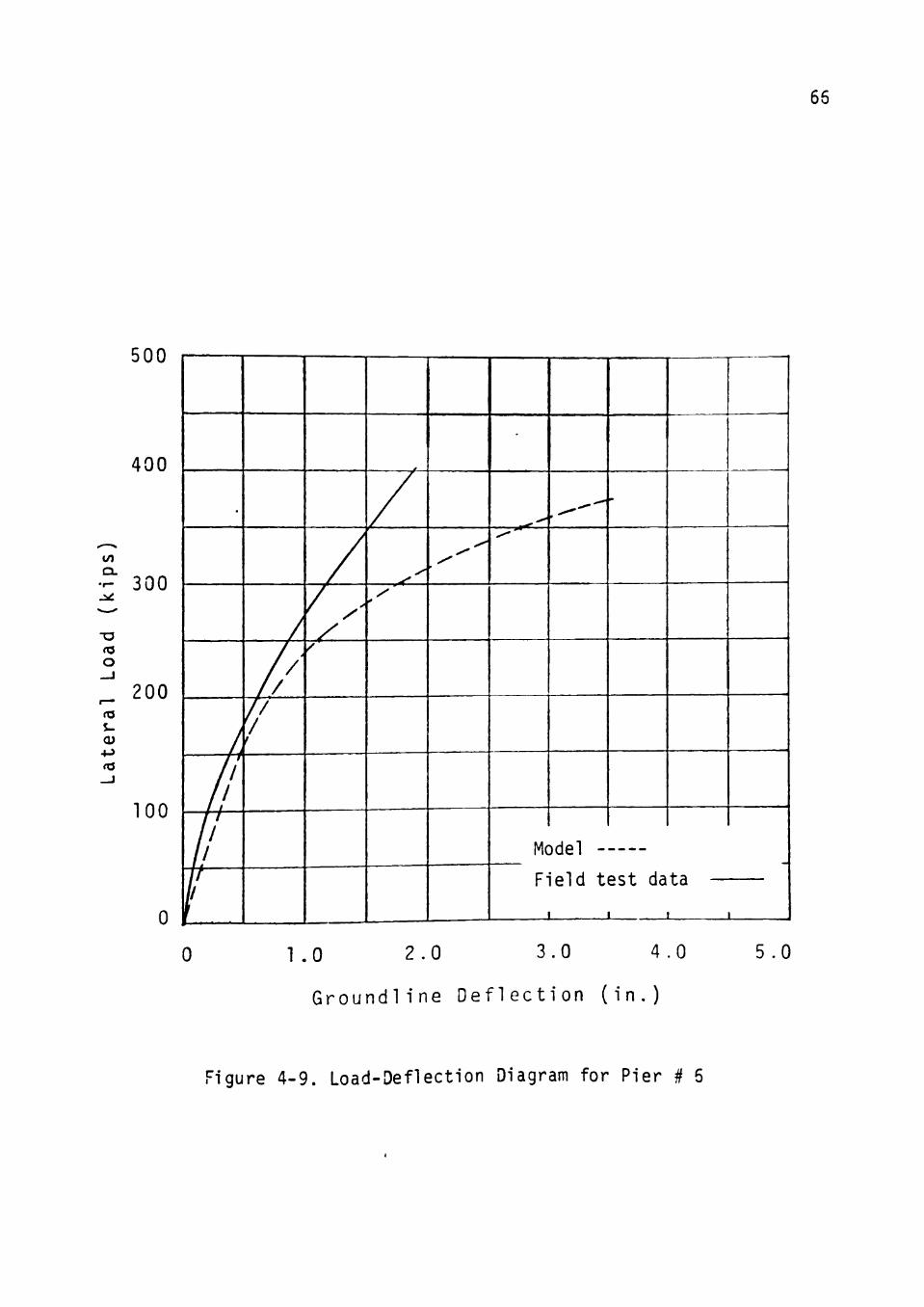
Example 6, Figure 4-9 , P i er # 6. This pier was t e s t e d ty
Bhushan , Haley, and Fong [ 2 ] - The pier dimensions and the
s o i l p r o p e r t i e s are as fo l l ows :
Pier dimensions : Length = 15.5 f t .
Diameter = 4 f t .
soil Properties are the same as for pier • 5 .
In this example, the predicted deflections are very
close to the actual deflections up to a load of about 250
k. At higher loads the results of the analysis deviate
from the actual test data conservatively.
66
500
400
to
- 300
-o O
200 CO S-(U
«o
100
0
.
—'h 1 1 1
/ / / /
/ / / /
/
/ / /
//
7
/ X
/^
y y*
y
y y
•
^ ^^
M(
F-
•
)del -
le 1 u c CO c u a
1
•l-T C U
r 1
0 1.0 2.0 3.0 4.0 5.0
Groundline Deflection (in.)
Figure 4-9. Load-Deflection Diagram for Pier # 6
67
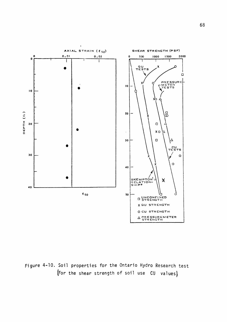
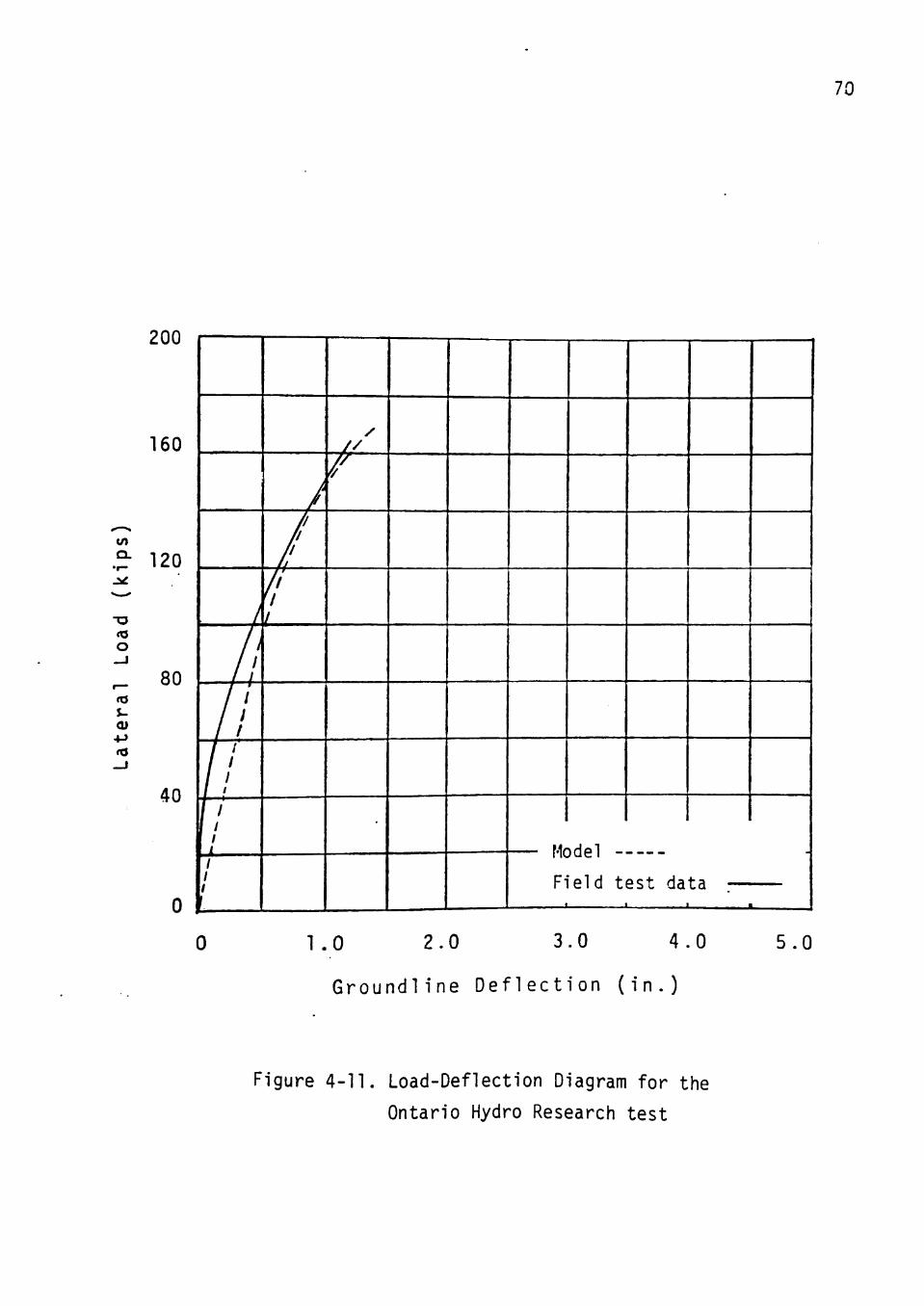
Example 7, Figure 4-11, the Ontario Hydro Research Tests
[9], the pier dimensions and the soil properties for this
test are as follows :
Pier dimensions : Length = 17 ft.
Diameter = 5 ft-
Has a 10 f t . diamter b e l l a t the
bottom 5 f t .
The a c t u a l s o i l propert i e s as published by Ismael and
Klym [ 9 ] are presented in Figure 4-10. Table 4-6 g i v e s the
a c t u a l v a l u e s of s o i l proper t i e s used in the computer
program.
In t h i s example, the e f f e c t of the bottom r e s i s t i n g
moment i s more than other examples which are s tud ied in
t h i s a n a l y s i s . The predicted d e f l e c t i o n s in t h i s c a s e are
very c l o s e to the ac tua l d e f l e c t i o n s up to the maximum load
of 160 k.
68
A X I A L . S T R A I N ( ( 5 0 )
0 . 0 1 0 . 0 2
S H E A R S T R E N G T H (P S F)
0 500 1000 1500 2000
I , « —
Q. U C
50 50
S K E M P T O N fi E L - A T I O N -SHI P *
-^ U N C O N F l N E D 'J S T R E N G T H
X Q U STI7 E N G T H
O CU S T R E N G T H
A P R E S S U R E M E T E R STR E N G T H
Figure 4-10. Soil properties for the Ontario Hydro Research test
[For the shear strength of soil use CU values)
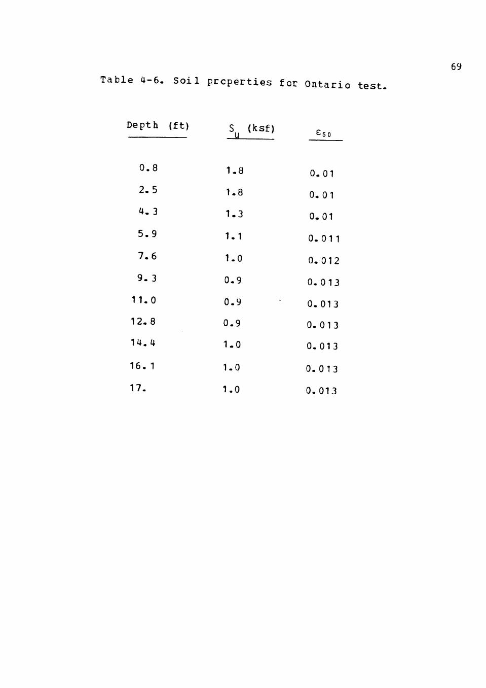
Table 4-6. Soil properties for Ontario test.
69
Depth (ft)
0.8
2.5
4. 3
5.9
7.6
9.3
11.0
12-8
14.4
16. 1
17.
s
1.8
1.8
1.3
1.1
1.0
0.9
0.9
0.9
1.0
1.0
1.0
(ksf)
•
^50
0.01
0.01
0.01
0.01 1
0.012
0. 013
0.013
0. 013
0.013
0. 0 13
0.013
200
160
Q. ? 120
T3 ea O
^ 80
40
1.0 2.0 3.0 4 .0
Ground l ine D e f l e c t i o n ( i n . )
70
/ / / /
/ / / /
/ / / / / / / / / /
/ / / / i / / / 1
A
// //
//
fi / /
7 /
/ /
ML Hol _
F I Q I / H +QC-t- /^a 1
1 •
w o o u a
— 1
¥~i . . _ .
•
5.0
Figure 4-11. Load-Deflection Diagram for the
Ontario Hydro Research test
Chapter 5
Conclusions and Recommendations
In t h i s s t u d y , a d i s c r e t e model for the a n a l y s i s cf
short p ier foundat ions i s developed. The fol lowing are the
b a s i c d i f f e r e n c e s between t h i s a n a l y s i s and previous
a n a l y s e s done by other i n v e s t i g a t o r s :
1. The p i e r i s assumed to be i n f i n i t e l y r i g i d .
2 . The concept of beam on e l a s t i c foundation i s not
used.
3 . Springs represent ing the bottom r e s i s t i n g moment,
bottom f r i c t i o n , bottom v e r t i c a l r e a c t i o n , and skin
f r i c t i o n are included in the model.
4 . The shear s t rength of s o i l ' i s not averaged over the
d i s tance from the ground surface to a depth X as was
done by Reese [ 2 0 ] .
5. The s o i l u l t i m a t e strength i s not modified as was
done by Ismael and Klym [ 9 ] .
71
72
The f o l l o w i n g c o n c l u s i o n s are der ived from t h i s s tudy :
1. The d i s c r e t e model p r e s e n t e d here has t h r e e d e g r e e s
of freedom, but i t r e p r e s e n t s t h e o v e r a l l behav ior
of t h e s o i l - s t r u c t u r e i n t e r a c t i o n .
2 . The l o a d - d i s p l a c e m e n t re sponse of the p i e r o b t a i n e d
us ing o n l y t h e l a t e r a l s p r i n g s n e g l e c t i n g t h e s k i n
f r i c t i o n and t h e bottom r e s i s t a n c e s , showed very
poor agreement with f i e l d t e s t d a t a .
3. The addit ion of the res i s t ing forces at the bottom
and on the s ides of the pier resulted in a more
r e a l i s t i c model, and the resu l t s of the analys i s
compared f a i r l y well with the f i e l d t e s t data fcr
most of the example problems.
4. The addition of b e l l to the pier increases the
e f f ec t of the bottom res is t ing moment and the bottom
f r i c t i o n a l force substant ia l ly , depending on the
s i z e of the be l l and the s o i l strength d i r e c t l y
below the b e l l .
5. In a few c a s e s , the predicted def lect ions of the
l a t e r a l l y loaded piers were not as c lose to the
•?3
ac tua l measured d e f l e c t i o n s as was des i r ed . This
may be because of pos s ib l e e r ro r in the measuremett
of the shear s t r eng th of so i l or the assumpt icrs
made in developing p-y curves and spring c o n s t a n t s .
6. The s i z e of the s t i f f n e s s matrix for t h i s model i s
only 3x3, no matter how many nodes on the p i e r are
chosen. This i s in con t r a s t to the prev ious ly
repor ted ana lyses where the s i z e of the s t i f f n e s s
matrix depended on the number of nodes which were
used as in the case of the team on e l a s t i c
foundat ion. Consequently , consider ing the non
l i n e a r nature of t h i s problem , the computer t i n e
requ i red to so lve the above system of equat ions over
and over u n t i l convergence is achieved i s reduced
cons iderably because in each i t e r a t i o n only a system
of th ree equat ions needs to be solved for the
unknowns.
^Recommendations for future s t ud i e s :
1. Ihe model can be programed on a oiinicomputer very
e a s i l y .
2. As more experimental data become a v a i l a b l e , the
74
model should be checked and spring constants revised
for obtaining better comparisons. For example, the
p-y curves need to be improved in order to be able
to determine the initial spring constants more
accurately and to represent its behavior at loads
close to its ultimate capacity.
3. A better knowledge and understanding of the soil
reactions (the bottom resisting moment, bottom
friction, and skin friction) through a series cf
tests and studies would be helpful to improve the
model.
5. The ana lys i s should be extended for sands and sandy
s o i l s .

R e f e r e n c e :
1 . Adams, v7. I . , and R a d h a k r i s h na, H . S . , "The L a t e r a l C a p a c i t y of Deep Augered F o o t i n g s , " P r o c e e d i n g s of t h e 8 th I n t e r n a t i o n a l C o n f e r e n c e of S o i l Mechanics a rd F o u n d a t i o n Engineering:! , V o l . 2 . 1 , Moscow, U . S . S . E . , 1973 , p p . 1-8-
2 . Bnushan , K . , H a l e y , S . C . , and Fong, P . T . , " L a t e r a l Load T e s t s on D r i l l e d P i e r s i n s t i f f C l a y s , " Tournal o r t h e G e o t e c h n i c a l E n g i n e e r i n g D i v i s i o n , Vo l . 105, NO. GTf, AUG., 1979 , P P . 9 6 9 - 9 6 5 .
3 . B o w l e s , J o s e p h E . , F o u n d a t i c n A n a l y s i s and D e s i g r , Second E d i t i o n , 1977, p p . 157-159 .
4 . Bowles , J o s e p h E . , F o u n d a t i o n A n a l y s i s and Des ign , Second E d i t i o n , 1977, p p . 8 2 - 8 7 .
5 . Broms, B. B. , " L a t e r a l R e s i s t a n c e of P i l e s in C o h e s i v e S o i l s , " jQurna 1 of t h e S o i l "1 ec ha n i c s ?.nd F o u n d a t i o n s D i v i s i o n , ASCE, Vol . 90 , No. SM2, P r o c . Paper 3825, M a r . , 19 6 4 , p p . 2 7 - 6 3 .
6» D o u g l a s , D . J . , and D a v i s , E . H . , "The Movement or Bur ied F o o t i n g s Due t o Moment and H o r i z o n t a l Load and t h e Movement o f Anchor P l a t e s , " G e o t e c h n i q u e , Vo l . 14, London, E n g l a n d , 1964, p p . 11 5-132.
7 . G i l l , H. L. ^ and Deraars, K. R. , " D i s p l a c e m e n t cf L a t e r a l l y Loaded S t r u c t u r e s i n N o n l i n e a r l y R e s p o n s i v e S o i l s , " T e c h n i c a l Report R670, Naval C i v i l E n g i n e e r i r g L a b o r a t o r y , P o r t Hueneume, C a l i f - , 1970 , pp. 1-59.
8 . Hansen , J . B . , "The U l t i m a t e R e s i s t a n c e of R ig id P i l e s A g a i n s t T r a n s v e r s F o r c e s . " Danish G e o t e c h n i c a l I n s t . , B u l l . 12 ( 1 9 6 1 ) .
9 . I s m a e l , N-F. , and ' lym, T. W., " B e h a v i o r of R i g i d P i e r s i n Layered C o h e s i v e S o i l s , " J o u r n a l of t h e G e o t e c h n i c a l E n g i n e e r i n g D i v i s i o n , ASCE, Vol . 104, No. GTS,Aug. , 1978 , p p . 1061-1074-
10. L a n d e r s , P h i l l i p , " R e s e a r c h on F o u n i a t i o n S y s t e m s , " J o u r n a l of t h e E l e c t r i c Power R e s e a r c h I n s t i t u t e , V o l . "4, No. 6 , J u l y / A u g u s t , 1979, pp. 3 3 - 3 4 .
75

75
11 .
12.
18.
L a n g h a a r , Henry L - , Energy Methods i n Appl ied Mechan ics . Viiley 5 S o n s , VJ62, pp - 1 - 3 3 .
M d t l o c k , H-, " C o r r e l a t i o n s for Design of L a t e r a l l y Loaded F i l e s in S o f t C l a y , " ^ r e p r i n t s , Second Annual O f f s h o r e Techno logy C o n f e r e n c e , ' l o u s t o n , T e x a s , V o l . No. OTC 1204, 1970 , p p . 1 - 5 7 7 - 5 8 8 .
I ,
13 . M c C l e l l a n d , B. , and F o c h t , J . A . , J r . , " S o i l Modulus f c r L a t e r a l l y Loaded P i l e s , " J o u r n a l of t h e S o i l ^ . echan ic s
20.
and Foundation Division, ASCE, Vol. 82, No. Paper 1081, Oct., 1956, pp.1-22.
S'fi'4 Proc-
14. McClelland, B., and Focht, J.A., Jr., discussion cf "Soil Modulus for Laterally Loaded Piles," ty McCelland, B. , and Focht, J.A-, Jr-, Transactions, ASCE. vol. 123, Paper No. 2954, 1950, p. 104:»-1086.
15. Poulos, H.G., "Behavior of Laterally Loaded Piles; I-single Piles," Journal of the Soil Mechanics and Foundations Division, ASCF, Vol. 97, Paper 8092, May, 1971, pp.71 1-731.
No. S M 5 , P r o c .
16» P o u l o s , H. G., "Behav io r of L a t e r a l l y Loaded P i l e s - I I I s o c k e t e d P i l e s , " J o u r n a l of t h e S o i l Mechanics ard F o u n d a t i o n s D i v i s i o n . ASCE, Vol. 9 8 , No. SM4, P r o c . P a p e r 8 8 3 7 , A p r . , 1972, pp . 341-360 .
17. R a d h a k r i s h n a , R . S . , "Highbury J e t t o London N o r t h e a s t TS , p r o p o s e d 230-KV 2 c c t S t e e l P o l e T r a n s m i s s i o n Line F u l l - s c a l e Founda t ion T e s t s , " O n t a r i o Hvdro R e s e a r c h D i v i s i o n P e £ o r t lo_. 71-4C9-K, T o r o n t o , Canada , 1971 ,
R e e s e , L . C - , d i s c u s s i o n of " S o i l Modulus f o r L a t e r a l l y Loaded P i l e s , " by B- McCle l l and , and J . A, F o c h t , J r . , T r a n s a c t i o n s . ASCE. Vol . 1 2 3 , Paper No. 2954 , 1 9 5 8 , pp . 1071-1074 .
19. R e e s e , L . C - , and Welch, R - C , " L a t e r a l Loading of '^eep " ~ "• "^ ^ ' - ' ^ e o t e c h n i c a l
GT7, P r o c . F o u n d a t i o n s i n s t i f f C l a y , " J o u r n a l of_ t h e E n g i n e e r i n g D i v i s i o n , H C E , Vol. 10 1 . No. p a p e r 11456, J u l y , 1975, pp
101 , 6 3 3 - 6 4 9 .
R e e s e , L. C. , Documenta t ion , " E n g i n e e r i r g Pi v i s i o n , ASCE, Vol-Paper 12862, A p r . , 1977, p p . 2 8 7 - 3 0 5 .
" L a t e r a l l y Loaded P i l e s : Program J o u r n a 1 of t h e G e o t e c h n i c a l
10 3 , No. G r 4 , P r c c .
77
21. Skeropton, A-l-J-, "The Bearing Capacity of Clays," Proceedings, Building Research Congress. Division 1, London,' England, 1951, pp. 180-188.
22. Stott, J. p.
23
H T e s t s on M a t e r i a l s f o r Use in S l i d i r g L a y e r s Under C o n c r e t e Road S l a b s , " c i v i l and P u b l i c Works R e v i e w , V o l . 5 6 , Nos . 1961 , p p . 1 2 9 7 , 1 2 9 9 , 1 3 0 1 , 1 4 6 6 , 1 6 0 3 , 1 6 0 5 .
E n g i n e e r inq 6 6 3 , 6 6 4 , 6 6 5 ,
Woodward , R i c h a r d J , , G a r d n e r , W i l l i a m S. , G r e e r , D a v i i M. , D r i l l e d P i e r F o u n d a t i o n s , M c G r a w - H i l l , I r . c . , 1972 , p p . 6 4 - 6 7 -