Embed Size (px)
Citation preview

A
Dirac’s delta Function
The 1-d delta function, δ(x), is defined through a limiting procedure so that
δ(x) = 0 for x = 0 (A.1a)
and δ(0) = ∞. The meaning of this last relation, taking into account (A.1a),is that ∫ b
a
dxf(x)δ(x) = f(0) (A.1b)
for any well-behaved function f(x) and for any pair a, b such that a < 0 < b.Some functions producing in the limit the delta function, as defined by
(A.1a, A.1b), are given below:
δ(x) =
⎧⎪⎪⎪⎪⎪⎪⎪⎪⎪⎪⎪⎪⎨⎪⎪⎪⎪⎪⎪⎪⎪⎪⎪⎪⎪⎩
limε→0+
1π
ε
x2 + ε2, Lorentzian, (A.2a)
limσ→0+
1σ√
2πexp
(− x2
2σ2
), Gaussian, (A.2b)
limε→0+
sin(x/ε)πx
, Dirichlet, (A.2c)
limL→∞
12π
∫ |L|
−|L|eikxdk , Fourier. (A.2d)
From the definition of the delta function it follows that
δ(g(x)) =∑
n
δ (x − xn)|g′ (xn)| , (A.3)
where g(x) is a well-behaved function of x, the sum runs over the real roots,xn, of g(x) = 0, and g′ (xn) ≡ (dg/dx)x=xn
= 0 for all xn.The derivative of the delta function is properly defined as
δ′(x) = 0 , x = 0 (A.4a)
338 A Dirac’s delta Function
and ∫ b
a
dxf(x)δ′(x) = −f ′(0) (A.4b)
for any well-behaved function f(x) and for any pair a, b such that a < 0 < b.The integral of the delta function is the so-called theta function
δ(x) =dθ(x)dx
, (A.5a)
where
θ(x) ≡
1 , for x > 0 ,
0 , for x < 0 . (A.5b)
The definition of the delta function is generalized to more than one inde-pendent cartesian variable:
δ (r) = δ (x1) δ (x2) . . . δ (xn) (A.6)
in an n-dimensional space. More explicitly we have
δ (r − r′) = δ (x − x′) δ (y − y′) =1r
δ (r − r′) δ (φ − φ′) , 2-d , (A.7)
δ (r − r′) = δ (x − x′) δ (y − y′) δ (z − z′)
=1r2
δ (r − r′) δ (cos θ − cos θ′) δ (φ − φ′)
=1
r2 sin θδ (r − r′) δ (θ − θ′) δ (φ − φ′) , 3-d . (A.8)
The completeness relation (1.4) of Chap. 1 allows us to obtain many seriesor integral representations of the delta function. For example, the Fourierrepresentation of the d-dimensional delta function is, according to (1.4) andthe footnote on p. 3,
δ (r − r′) =∑
k
φk (r)φ∗k (r′) =
1Ω
∑k
eik · (r−r′) −→Ω→∞
=1Ω
Ω
(2π)d
∫dkeik · (r−r′) =
1(2π)d
∫dkeik · (r−r′) . (A.9)
Equation (A.9) generalizes in d-dimensions (A.2d).Similarly, the delta function over the spherical angles θ and φ can be
expressed as a sum over spherical harmonics, Ym(θ, φ), according to (1.4):
δ (cos θ − cos θ′) δ (φ − φ′) =1
sin θδ (θ − θ′) δ (φ − φ′)
=∞∑
=0
∑m=−
Ym(θ, φ)Y ∗m (θ′, φ′) , (A.10)

A Dirac’s delta Function 339
where the spherical harmonics are given in terms of the associated Legendrepolynomials, P
|m| , by the following expression:
Ym(θ, φ) = i(−1)(|m|+m)/2
√(2 + 1)( − |m|)!
4π( + |m|)! P|m| (cos θ)eimφ . (A.11)
Equation (A.10) is valid because the set Ym(θ, φ) is orthonormal∫ π
0
sin θdθ
∫ 2π
0
dφY ∗m(θ, φ)Y′m′(θ, φ) = δ′δmm′ .
B
Dirac’s bra and ket Notation
In quantum mechanics, the states of a particle are described by eigenfunctions,φn (r), of any hermitian operator,L, corresponding to a physical quantity suchas its momentum, its Hamiltonian, etc. The same physical states can equallywell be described by the Fourier transforms, φn (k), of φn (r) or by any otherrepresentation of φn (r) such as the set an, of the expansion
φn (r) =∑
an,ψ (r) (B.1)
in terms of a complete orthonormal set of functions ψ.It is very convenient to introduce for a physical state a single symbol that
will be independent of any particular representation and such that the variousrepresentations, φn (r), φn (k), and an,, can be reproduced easily wheneverthey are needed. This symbol is denoted by |n〉 or by |φn〉 and is called a ket.Thus
State of a particle characterized by quantum number(s) n ⇐⇒ |φn〉 or |n〉To each ket |φn〉 corresponds one and only one conjugate entity denoted
by 〈φn| and called a bra. We define also the inner product of two kets, |φ〉 and|ψ〉, (in that order) as a complex quantity denoted by 〈φ |ψ〉 and such that
〈φ |ψ〉∗ = 〈ψ |φ〉 . (B.2)
In particular, for an orthonormal set we have
〈φn |φm〉 = δnm . (B.3)
Physically, the inner product 〈φ |ψ〉 gives the probability amplitude for a par-ticle being in state |ψ〉 to be observed in state |φ〉.
A complete set of kets, |φn〉, defines an abstract Hilbert space. Someusual complete sets of kets for a spinless particle are the following:
(a) The position kets |r〉, where r runs over all positions in the domain Ω;|r〉 corresponds to the state where the particle is completely localized atthe point r.

342 B Dirac’s bra and ket Notation
(b) The momentum kets |k〉; |k〉 corresponds to the state where the particlehas momentum k.
(c) The Bloch kets |k, n〉; |k, n〉 corresponds to the state where the particlehas crystal momentum k and belongs to the nth band.
(d) The kets |φ〉; |φ〉 is an eigenstate of the Hamiltonian. The indexesfully characterize this eigenstate.
According to the above, the inner product 〈r |ψ〉 gives the probability ampli-tude for a particle being in the state |ψ〉 to be observed at the point r; butthis probability amplitude is nothing other than ψ (r). Hence
ψ (r) = 〈r |ψ〉 . (B.4)
Similarly,ψ (k) = 〈k |ψ〉 . (B.5)
If in (B.4) we choose |ψ〉 = |k〉, then we obtain
〈r |k〉 =1√Ω
eik · r . (B.6)
The rhs is the r-representation of a normalized plane wave; if in (B.4) wechoose |ψ〉 = |r′〉, then we have
〈r | r′〉 = δ (r − r′) . (B.7)
Equation (B.7) follows from the orthonormality of the set |r〉.From (B.4) and (B.7) we obtain
ψ (r) = 〈r |ψ〉 =∫
dr′δ (r − r′) 〈r′ |ψ〉 =∫
dr′ 〈r | r′〉 〈r′ |ψ〉
= 〈r|∫
dr′ |r′〉 〈r′ |ψ〉 . (B.8)
Since (B.8) is valid for every 〈r| and every |ψ〉, we end up with the complete-ness relation for the set |r′〉:∫
dr′ |r′〉 〈r′| = 1 . (B.9)
Similarly, we obtain the relation
1 =∑
k
|k〉 〈k| −→Ω→∞
Ω
(2π)d
∫dk |k〉 〈k| . (B.10)
Using (B.9) and (B.10) we can easily transform from ψ(r) to ψ (k) and viceversa
ψ (k) = 〈k |ψ〉 =∫
dr 〈k |r〉 〈r |ψ〉 =∫
dr1√Ω
e−ik · rψ (r)
=1√Ω
∫dre−ik · rψ (r) , (B.11)

B Dirac’s bra and ket Notation 343
ψ (r) = 〈r |ψ〉 =∑
k
〈r |k〉 〈k |ψ〉 =1√Ω
∑k
eik · rψ (k)
=√
Ω
(2π)d
∫dkeik · rψ (k) . (B.12)
Notice that the definition of the inner product coincides with the usual defi-nition in the r-representation:
〈φ |ψ〉 =∫
dr 〈φ | r〉 〈r |ψ〉 =∫
drφ∗ (r)ψ (r) . (B.13)
The form of any operator in the Dirac notation follows by calculating itsmatrix elements. For example, taking into account that the position opera-tor, r, satisfies by definition the relation 〈r| r = 〈r| r and that the momentumoperator, p, satisfies the relation 〈k| p = 〈k|k, we have
〈r | r |ψ〉 = r 〈r |ψ〉 = rψ (r) , (B.14)
〈k | p |ψ〉 = k 〈k |ψ〉 = kψ (k) . (B.15)
Using (B.10) and (B.15) we obtain the matrix element 〈r | p |ψ〉:
〈r | p |ψ〉 =∑
k
〈r |k〉 〈k | p |ψ〉 =∑
k
1√Ω
eik · rkψ (k)
=∑
k
−i∂
∂reik · r 1√
Ωψ (k) = −i
∂
∂r
∑k
1√Ω
eik · rψ (k)
= −i∂
∂rψ (r) . (B.16)
The last relation follows from (B.12). In a similar way one can show that
〈k | r |ψ〉 = i∂
∂kψ (k) . (B.17)
The relations (B.14)–(B.17) can be generalized for operators that are func-tions of r or p. Since by definition the function f
(A)
of any operator A is
an operator with the same eigenstates as A and eigenvalues f (Ai), where Ai
are the eigenvalues of A, we have
〈r | f (r) |ψ〉 = f∗ (r)ψ (r) , (B.18)
〈k | g (p) |ψ〉 = g∗ (k) ψ (k) , (B.19)
〈r | g (p) |ψ〉 = g∗(−i
∂
∂r
)ψ (r) , (B.20)
〈k | f (r) |ψ〉 = f∗(
i∂
∂k
)ψ (k) . (B.21)

344 B Dirac’s bra and ket Notation
For hermitian operators f∗ (r) = f (r) and g∗ (k) = g (k). As an applicationof (B.18) and (B.20) we have⟨
r
∣∣∣∣∣ p2
2m+ V (r)
∣∣∣∣∣ψ⟩
=[−
2
2m∇2
r + V (r)]
ψ (r) . (B.22)
For particles with spin 1/2 we have to specify whether the spin is up (↑) ordown (↓). Thus a complete set is |r, ↑〉 , |r, ↓〉 or |k, ↑〉 , |k, ↓〉. Assumingthat the spin quantization axis is the z-axis, we have for the spin operators = x0sx + y0sy + z0sz:
sz |r, σ〉 =12σ |r, σ〉 ,
σ = +1 for spin up ,σ = −1 for spin down , (B.23)
∣∣∣∣ 〈r, ↑ | s |ψ〉〈r, ↓ | s |ψ〉
∣∣∣∣ =12σ
∣∣∣∣ 〈r, ↑ |ψ〉〈r, ↓ |ψ〉
∣∣∣∣ , (B.24)
where σ is the vector defined by the three Pauli matrices
σ =(
0 11 0
)x0 +
(0 −ii 0
)y0 +
(1 00 −1
)z0 . (B.25)

C
Solutions of Laplace and Helmholtz Equations
in Various Coordinate Systems1
C.1 Helmholtz Equation (∇2 + k2) ψ (r) = 0
C.1.1 Cartesian Coordinates x, y, z
ψ (r) =∑m
Am [sin (x1) + b cos (x1)]
×[sinh
(√2 + m2x2
)+ cm cosh
(√2 + m2x2
)]×[sin
(√m2 + k2x3
)+ dm cos
(√m2 + k2x3
)]. (C.1)
The set x1, x2, x3 represents any permutation of the set x, y, z. Bound-ary conditions (BCs) and normalization may fully determine the variouseigensolutions and eigenvalues. Instead of sin (x1) + b cos (x1), one can useexp (ix1)+ b′ exp (−ix1); similar replacements can be employed in the otherfactors of (C.1).
The solution of the Laplace equation ∇2φ = 0 is obtained immediately bysetting k = 0 in (C.1).
C.1.2 Cylindrical Coordinates z, φ,
ψ (r) =∑m,n
Amn [sinh(mz) + bm cosh(mz)] [sin(nφ) + cn cos(nφ)]
×[Jn
(√m2 + k2
)+ dnmYn
(√m2 + k2
)]. (C.2)
In the first factor of the rhs of (C.2) one can use instead of sinh(mz) +bm cosh(mz) the sum emz + b′me−mz. Similarly, in the second factor one canuse einφ + c′ne−inφ. Finally, in the last factor one may use
H(1)n (w) = Jn(w) + iYn(w)
1 For the definition and properties of the most common special functions see [1].

346 C Laplace and Helmholtz Equations
and/orH(2)
n (w) = Jn(w) − iYn(w)
instead of Jn and Yn, where w =√
m2 + k2. Recall that
Jn(w) → (w/2)n
Γ (n + 1), w → 0 , n = −1,−2, . . . , (C.3a)
Yn(w) → − 1π
Γ (n)(w/2)−n , w → 0 , Re n > 0 , (C.3b)
Y0(w) → 2π
lnw + const. , w → 0 , (C.3c)
H(1)n (w) →
√2
πwei(w−nπ/2−π/4) , w → ∞ , (C.3d)
H(2)n (w) →
√2
πwe−i(w−nπ/2−π/4) , w → ∞ . (C.3e)
Thus, Yn(w) blows up for w → 0; H(1)n (w) and H
(2)n (w) represent for w → ∞
outgoing and ingoing waves, respectively, while for Im w > 0, H(1)n (w) and
H(2)n (w) blow up as w → 0.The solution of the Laplace equation, ∇2φ = 0, is obtained by setting k = 0
in (C.2). The solutions of the Helmholtz equation in 2-d polar coordinates, φand , are produced by setting m = 0 in (C.2). Finally, for the solution of theLaplace equation in 2-d polar coordinates, we must take m = 0 and k → 0 sothat
φ (r) =∑n=0
An [sin(nφ) + cn cos(nφ)](n + dn−n
)+A0 (1 + d0 ln ) . (C.4)
C.1.3 Spherical coordinates r, θ, φ
ψ (r) =∑m
Am
(eimφ + bme−imφ
)[Pm
(cos θ) + cmQm (cos θ)]
× [j(kr) + dy(kr)] . (C.5)
Qm (cos θ) is singular for θ = 0 and θ = π; similarly, Pm
(cos θ) is singular forθ = 0 and θ = π unless is a nonnegative integer. Thus, cm must be zeroand must a nonnegative integer if θ = 0 or π is included in the problem.
The spherical Bessel functions, j(w) and y(w), are defined by the rela-tions
j(w) =√
π
2wJ+ 1
2(w)
→ w
1 × 3 × · · · × (2 + 1)as w → 0 , (C.6a)

C.2 Vector Derivatives 347
y(w) =√
π
2wY+ 1
2(w)
→ −1 × 3 × · · · × (2 − 1)w+1
as w → 0 . (C.7a)
In a similar way we define the spherical Hankel functions h(1) (w) = j(w)+
iy(w) and h(2) (w) = j(w) − iy(w), which represent outgoing and ingoing
spherical waves, respectively.For problems covering the full range of values of φ (0 ≤ φ ≤ 2π) and
θ (0 ≤ θ ≤ π), cm must be set equal to zero, must be a nonnegative integerfor the reasons explained above, m must be an integer running from − to +,and the first two factors in brackets on the rhs of (C.5) are then represented bythe spherical harmonic Ym(θ, φ) [not to be confused with the Bessel functionYn(w)] given by (A.11) in Appendix A. The set Ym(θ, φ) is an orthonormalcomplete set of functions over the whole surface of the 3-d unit sphere.
The solution of the Laplace equation, ∇2φ = 0, is obtained by taking thelimit k → 0 in (C.5) and using (C.6a) and (C.7a):
φ (r) =∑m
Am
[eimφ + bme−imφ
]× [Pm
(cos θ) + cmQm (cos θ)]
(r + d′/r+1
). (C.8)
If φ and θ cover the full range of their values, then the first two factors inbrackets on the rhs of (C.8) must be replaced by Ym(θ, φ), as given by (A.11).
C.2 Vector Derivatives
We shall conclude this Appendix by giving the formulae for some vector deriva-tives in spherical and cylindrical coordinates.
C.2.1 Spherical Coordinates r, θ, φ
gradψ (r) ≡ ∇ψ (r) =∂ψ
∂θir +
1r
∂ψ
∂θiθ +
1r sin θ
∂ψ
∂φiφ . (C.9)
divA (r) ≡ ∇ ·A (r)
=1r2
∂
∂r
(r2Ar
)+
1r sin θ
∂
∂θ(sin θAθ) +
1r sin θ
∂Aφ
∂φ. (C.10)
∇2ψ (r) =1r2
∂
∂r
(r2 ∂ψ
∂r
)+
1r2 sin θ
∂
∂θ
(sin θ
∂ψ
∂θ
)+
1r2 sin2 θ
∂2ψ
∂φ2. (C.11)

348 C Laplace and Helmholtz Equations
C.2.2 Cylindrical Coordinates z, , φ
gradψ (r) ≡ ∇ψ (r) =∂ψ
∂ziz +
∂ψ
∂i +
1
∂ψ
∂φiφ . (C.12)
divA (r) ≡ ∇ ·A (r) =∂Az
∂z+
1
∂
∂(A) +
1
∂Aφ
∂φ. (C.13)
∇2ψ (r) =∂2ψ
∂z2+
1
∂
∂
(∂ψ
∂
)+
12
∂2ψ
∂φ2. (C.14)
C.3 Schrodinger Equation in Centrally Symmetric3- and 2-Dimensional Potential V
− 2
2m∇2ψ + V ψ = Eψ . (C.15)
For the 3-d case we write
ψ (r) =u(r)
rYm(θ, φ), (C.16)
and we obtain
− 2
2m
d2u
dr2+[V (r) +
2( + 1)2mr2
]u = Eu , (C.17a)
(r × p)2 = −2 (r ×∇)2
= −2
[1
sin2 θ
∂2
∂φ2+
1sin θ
∂
∂θ
(sin θ
∂
∂θ
)], (C.17b)
(r × p)2 Ym (θ, φ) = 2( + 1)Ym(θ, φ) , (C.17c)
where Ym(θ, φ) is given by (A.11); in particular,
Y0(θ, φ) = i√
2 + 14π
P(cos θ) . (C.17d)
Equation (C.17a) is a 1-d Schrodinger equation with an effective potentialconsisting of the actual potential V (r) plus the centrifugal part; the latterequals the eigenvalue,
2( + 1), of the square of the angular momentum,r × p, over twice the “moment of inertia” mr2.
For the 2-d polar coordinates we write
ψ (r) = R()Φ(φ) , (C.18)
and we obtainΦ(φ) = einφ + bne−inφ (C.19a)

C.3 Schrodinger Equation 349
and
2 d2R
d2+
dR
d+ R
[(2mE
2− 2mV ()
2
)2 − n2
]= 0 . (C.19b)
If V () is a constant such that E − V > 0, we define k2 = 2m(E − V )/2
and (C.19b) becomes the ordinary Bessel equation with solutions Jn(k) andYn(k) [see (C.2) for m = 0].
If V () is a constant such that E − V < 0, then we define −k2 =2m(E −V )/
2, and (C.19b) becomes the modified Bessel equation with solu-tions In(k) and Kn(k) satisfying the following relations:
In(w) =
e−inπ/2Jn(iw), −π < argw ≤ π/2 ,e3inπ/2Jn(iw), π/2 < arg w ≤ π ; (C.20)
Kn(w) =
⎧⎪⎨⎪⎩iπ2
einπ/2H(1)n (iw), −π < argw ≤ π/2 ,
− iπ2
e−inπ/2H(2)n (−iw), π/2 < arg w ≤ π . (C.21)
Other useful properties of In(w) and Kn(w) are given in [1].
D
Analytic Behavior of G(z) Near a Band Edge
The Green’s function G(z) can be expressed in terms of the discontinuityG(E) ≡ G+(E) − G−(E) as follows:
G(z) =i
2π
∫ ∞
−∞dE
G(E)z − E
. (D.1)
The derivative of G(z) is obtained by differentiation under the integral. Inte-grating by parts we obtain
G′(z) =i
2π
∫ ∞
−∞dE
G′(E)z − E
, (D.2)
where the prime denotes differentiation with respect to the argument. In ob-taining (D.2) we have assumed that G′(E) exists and is integrable and thatG(E)/E → 0 as |E| → ∞. By taking the limits Im z → 0± and using (1.20)we obtain
G±(E) =i
2πP∫ ∞
−∞dE′ G(E′)
E − E′ ±12G(E) , (D.3)
ddE
G±(E) =i
2πP∫ ∞
−∞dE′ G
′(E′)E − E′ ±
12G′(E) , (D.4)
where one can show under the above assumptions that
G′(z) −→Imz→0±
ddE
G±(E) .
We would like to connect the behavior of G(z) and G′(z) as z → E0 withthe behavior of G(E) around E0. One can prove the following theorems [15]about F (z) given by
F (z) =i
2π
∫ ∞
−∞dx
f(x)z − x
=1
2πi
∫ ∞
−∞
f(x)x − z
dx . (D.5)

352 D Analytic Behavior of G(z) Near a Band Edge
Theorem 1. If f(x) satisfies the condition
|f (x1) − f (x2)| ≤ A |x1 − x2|µ (D.6)
for all x1 and x2 in the neighborhood of x0, where A and µ are positive con-stants, then
|F (z1) − F (z2)| ≤ A′ |z1 − z2|µ when µ < 1 , (D.7)
and|F (z1) − F (z2)| ≤ A′ |z1 − z2|1−ε when µ = 1 , (D.8)
for all z1 and z2 in the neighborhood of x0 and Im z1 Im z2 > 0; A′ isa positive constant and ε is an arbitrary positive number.
Inequalities (D.7) and (D.8) are valid as one or both of z1 and z2 reach thereal axis either from above or from below. Thus, e.g.,∣∣F+ (x1) − F+ (x2)
∣∣ ≤ A′ |x1 − x2|µ when µ < 1 , (D.9)
with a similar relation for F−(x1) − F−(x2).
Theorem 2. If f(x) is discontinuous at x = x0, i.e.,
f(x+
0
)− f(x−
0
)= D = 0 , (D.10)
but otherwise f(x) satisfies condition (D.6) for both x1 and x2 being either tothe left or to the right of x0, then
F (z) =D
2πiln(
1x0 − z
)+ F0(z) , (D.11)
where F0(z) satisfies (D.7) or (D.8).
Theorem 3. If f(x) behaves around x0 as
f(x) = f0(x) + f1(x)θ (±x ∓ x0) [±x ∓ x0]−γ
, (D.12)
where f0(x) and f1(x) satisfy condition (D.6) and 0 < γ < 1, then
F (z) = ± e±γπi
2i sin(γπ)f1(x0)
(±z ∓ x0)γ + F0(z) , (D.13)
where (±z ∓ x0)−γ is the branch that coincides with the branch (±x ∓ x0)
−γ
in (D.12) as z approaches x from the upper half-plane and
|F0(z)| <C
|z − x0|γ0 , (D.14)
where C and γ0 are positive constants such that γ0 < γ.

D Analytic Behavior of G(z) Near a Band Edge 353
The above theorems allow us to obtain the analytic behavior of G(z) neara band edge. Thus:
(a) When G(E) goes to zero as (E − EB)µ (µ > 0) near the band edge EB ,then, according to Theorem 1 above, G(z) and G±(E) are bounded in theneighborhood of EB. The derivatives G′(z) and G±′
(E) can be obtainedusing (D.2). Since G′(E) behaves as (E − EB)µ−1 inside the band andnear the band edge, then, according to Theorem 3 above, the quantitiesG′(z) and G±′
(E) behave as (z − EB)µ−1 and (E − EB)µ−1 as z and Eapproach EB. For a free particle in 3-d, µ = 1/2.
(b) When G(E) goes to zero in a discontinuous way at the band edge (as inthe 2-d free-particle case), one can apply Theorem 2 above. Consequently,G(z) and G±(E) exhibit a logarithmic singularity as shown in (D.11).
(c) When G(E) behaves as |E − EB|−γ with 0 < γ < 1 in the interior of theband and near the band edge EB, then, according to Theorem 3 above,G(z) and G±(E) behave as (z−EB)−γ and (E−EB)−γ , respectively. Fora free particle in 1-d, γ = 1/2.

E
Wannier Functions
For many purposes it is useful to introduce the Wannier functions. The Wan-nier function associated with the band index n and the lattice site is definedas [27, 28, 30]
wn (r − ) =1√N
∑k
e−ik · ψnk (r) , (E.1)
where ψnk (r) are the Bloch eigenfunctions given by (5.2). The Wannier func-tions wn (r − ) are localized around the lattice site .
The functions wn (r − ) for all n and form a complete orthonormalset; thus any operator, e.g., the Hamiltonian, can be expressed in a Wannierrepresentation. It may happen that the eigenenergies associated with a par-ticular band index n0 are well separated from all the other eigenenergies. Inthis case the matrix elements of the Hamiltonian H between wn0 (r − ) andwn (r − m), where n = n0, may be much smaller than |εn − εn0 |. Then thesesmall matrix elements to a first approximation can be omitted, and the sub-space spanned by the states wn0 (r − ), where runs over all lattice vectors,becomes decoupled from the rest. Let us assume that the band n0 is associatedwith a single atomic orbital φ (r − ) per atom; then, the set wn0 (r − ) isnothing other than an orthonormalized version of the set φ (r − ). If thelatter is assumed to be orthonormal, then the Wannier functions wn0 (r − )and the atomic orbitals φ (r − ) coincide. However, in general, the Wannierfunctions are hybridized atomiclike orbitals that possess two important fea-tures: completeness and orthonormality.

F
Renormalized Perturbation Expansion (RPE)
Consider the tight-binding Hamiltonian H = H0 + H1, where
H0 =∑
|〉 ε 〈| , (F.1)
H1 = V∑m
′ |〉 〈m| , (F.2)
and the summation in (F.2) extends over nearest-neighbor sites only. If weconsider H0 as the unperturbed Hamiltonian and H1 as a perturbation, we canapply the formalism developed in Chap. 4. Thus we have for G(z) ≡ (z−H)−1
G = G0 + G0H1G0 + G0H1G0H1G0 + · · ·or
G (, m) = G0 (, m) +∑
n1n2
G0 (, n1) 〈n1 | H1 |n2〉G0 (n2, m)
+∑
n1...n4
G0 (, n1) 〈n1 | H1 |n2〉G0 (n2, n3)
× 〈n3 | H1 |n4〉G0 (n4, m)+ · · · . (F.3)
It is clear from (F.1) that G0 (n1, n2) = δn1n2G0 (n1), where G0 (n) is
G0 (n) =1
z − εn. (F.4)
Similarly, 〈n1 | H1 |n2〉 is different from zero only when n1 and n2 are nearestneighbors. Hence (F.3) can be simplified as follows:
G (, m) = δ,mG0 () + G0()V G0 (m) δ,m+1
+∑n1
G0 ()V G0 (n1)V G0 (m) + · · · . (F.5)
358 F Renormalized Perturbation Expansion (RPE)
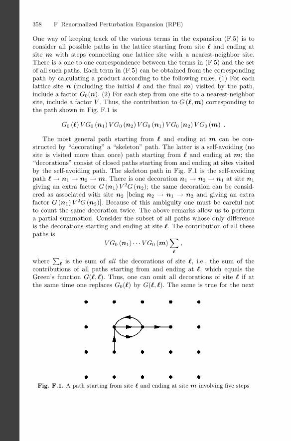
One way of keeping track of the various terms in the expansion (F.5) is toconsider all possible paths in the lattice starting from site and ending atsite m with steps connecting one lattice site with a nearest-neighbor site.There is a one-to-one correspondence between the terms in (F.5) and the setof all such paths. Each term in (F.5) can be obtained from the correspondingpath by calculating a product according to the following rules. (1) For eachlattice site n (including the initial and the final m) visited by the path,include a factor G0(n). (2) For each step from one site to a nearest-neighborsite, include a factor V . Thus, the contribution to G (, m) corresponding tothe path shown in Fig. F.1 is
G0 () V G0 (n1)V G0 (n2)V G0 (n1)V G0 (n2)V G0 (m) .
The most general path starting from and ending at m can be con-structed by “decorating” a “skeleton” path. The latter is a self-avoiding (nosite is visited more than once) path starting from and ending at m; the“decorations” consist of closed paths starting from and ending at sites visitedby the self-avoiding path. The skeleton path in Fig. F.1 is the self-avoidingpath → n1 → n2 → m. There is one decoration n1 → n2 → n1 at site n1
giving an extra factor G (n1)V 2G (n2); the same decoration can be consid-ered as associated with site n2 [being n2 → n1 → n2 and giving an extrafactor G (n1)V 2G (n2)]. Because of this ambiguity one must be careful notto count the same decoration twice. The above remarks allow us to performa partial summation. Consider the subset of all paths whose only differenceis the decorations starting and ending at site . The contribution of all thesepaths is
V G0 (n1) · · ·V G0 (m)∑
,
where∑
is the sum of all the decorations of site , i.e., the sum of thecontributions of all paths starting from and ending at , which equals theGreen’s function G(, ). Thus, one can omit all decorations of site if atthe same time one replaces G0() by G(, ). The same is true for the next
Fig. F.1. A path starting from site and ending at site m involving five steps

F Renormalized Perturbation Expansion (RPE) 359
site n1, but with one difference: decorations of site n1 that visit site must beomitted because these decorations have been included already as decorationsassociated with site . The decorations at site n1 can be omitted if G0(n1)is replaced by G (n1, n1 []), where the symbol [] denotes that in evaluatingG (n1, n1 []) the paths visiting site must be excluded. This exclusion isobtained automatically if one assumes that ε = ∞ [because then G0() = 0].Hence, G (n1, n1 []) is the n1, n1 matrix element of H with ε = ∞. Similarly,all the decorations at site n2 can be omitted if at the same time one replacesG0(n2) by G (n2, n2 [, n1]), where the symbol [, n1] denotes that both ε
and εn1 are infinite. This way one avoids double counting decorations passingthrough n2 that have been already counted as decorations associated withsite or site n1. As a result of these partial summations one can write forG (, m)
G (, m) =∑
G(, )V G (n1, n1 [])V
× G (n2, n2 [, n1]) V · · ·V G (m, m [, n1, n2, . . .]) , (F.6)
where the summation is over all self-avoiding paths starting from and endingat m, → n1 → n2 → · · · → m. In particular, for the diagonal matrixelements G(, ) we have
G(, ) = G0 () +∑
G(, )V G (n1, n1 [])V · · ·G0 () , (F.7)
where again the summation extends over all closed self-avoiding paths startingfrom and ending at . The last factor is G0 () because all decorations of thefinal site have already been counted as decorations of the initial site .Equation (F.7) can be rewritten as
G(, ) = G0 () + G(, )∆ ()G0 () , (F.8)
where ∆ () is called the self-energy1 and is given by
∆ () =∑
V G (n1, n1 [])V · · ·V . (F.9)
Equation (F.8) can be solved for G(, ) to give
G(, ; z) =G0 ()
1 − G0 ()∆ (; z)=
1z − ε − ∆ (; z)
. (F.10)
The last step follows from (F.4). Equation (F.10) justifies the name self-energy for ∆ (). The expansions (F.6), (F.7), and (F.9) for G (, m), G(, ),and ∆ (), respectively, are called the renormalized perturbation expansions(RPEs), [388,445,446]. Their characteristic property is that they involve sum-mation over terms that are in one-to-one correspondence with the self-avoiding1 The name self-energy is used in the literature for different quantities depending
on the forms of H0 and H1.

360 F Renormalized Perturbation Expansion (RPE)
paths in the lattice. The price for the simplification of having self-avoidingpaths is that the factors associated with lattice sites are complicated Green’sfunctions of the type G (n, n [, n1, . . .]). These Green’s functions can be eval-uated by using again the RPE. One can iterate this procedure. Note that fora system involving only a finite number of sites, the summations associatedwith the RPE involve only a finite number of terms. The iteration procedureterminates also, since with every new step in the iteration at least one ad-ditional site is excluded. Thus, the RPE iterated as indicated above gives aclosed expression for the Green’s functions of a system involving a finite num-ber of sites. For a system having an infinite number of sites the terms in eachsummation and the steps in the iteration procedure are infinite; thus for aninfinite system the question of the convergence of the RPE arises.
The RPE can be used very successfully to calculate Green’s functions forBethe lattices. For the double periodic case shown in Fig. 5.11, we have forthe self-energy ∆()
∆() = (K + 1)V 2G( + 1, + 1[]) , (F.11)
since there are only K + 1 self-avoiding paths starting from and ending atsite (each one visiting a nearest neighbor). The quantity G( + 1, + 1[])can be written according to (F.10) as
G( + 1, + 1[]) =1
z − ε+1 − ∆( + 1[]). (F.12)
Using the RPE, the self-energy ∆( + 1[]) can be written as
∆( + 1[]) = KV 2G( + 2, + 2[ + 1]) . (F.13)
We use K and not (K + 1) since the self-avoiding path involving site isexcluded. By combining (F.12) and (F.13), we have
G( + 1, + 1[]) =1
z − ε+1 − KV 2G( + 2, + 2[ + 1]). (F.14)
Similarly,
G( + 2, + 2[ + 1]) =1
z − ε+2 − KV 2G( + 3, + 3[ + 2]). (F.15)
Because of the periodicity shown in Fig. 5.11, G( + 3, + 3[ + 2]) = G( +1, + 1[]). Thus (F.14) and (F.15) become a set of two equations for the twounknown quantities G(+1, +1[]) and G(+2, +2[+1]) = G(, [+1]).By solving this system we obtain
G( + 1, + 1[])
=(z − ε1) (z − ε2) −
√(z − ε1) (z − ε2) [(z − ε1) (z − ε2) − 4KV 2]
2K (z − ε+1)V 2, (F.16)
G(, [ + 1])
=(z − ε1) (z − ε2) −
√(z − ε1) (z − ε2) [(z − ε1) (z − ε2) − 4KV 2]
2K (z − ε)V 2. (F.17)

F Renormalized Perturbation Expansion (RPE) 361
Substituting in (F.11) and (F.10) we obtain for G(, ) the expression givenin (5.57) and (5.58).
For the calculation of the off-diagonal matrix element, G(, m), one canapply (F.6). For a Bethe lattice there is just one self-avoiding diagram con-necting site with site m; G( + 1, + 1[]) has already been calculated, andG( + 2, + 2[, + 1]) equals G( + 2, + 2[ + 1]), which has been evaluated.These two quantities alternate as we proceed along the sites of the uniquepath connecting with m. Thus one obtains the expressions (5.59a), (5.59b),and (5.60) for G(, m).
We mention without proof two theorems concerning products of the form
P = G(, , z)G (n1, n1 [] ; z)×G (n2, n2 [, n1] ; z) · · ·G (m, m [, n1, n2 . . .] ; z) .
The first states that
P =
∏i
(z − Eai )∏
j
(z − Ej), (F.18)
where Eai is the eigenenergies of H with sites , n1, n2, . . . ,m removed, i.e.,
ε = εn1 = εn2 = · · · = εm = ∞, and Ej is the eigenenergies of H. Thesecond theorem states that
P = detG , (F.19)
where G is a matrix with matrix elements G(s, r, z), where both s and rbelong to the set , n1, n2, . . .m.

G
Boltzmann’s Equation
The function to be determined by employing Boltzmann’s equation (BE) isthe density, f (r, k; t), of particles in phase space, defined by the relation
dN ≡ (2s + 1)ddr ddk
(2π)df (r, k; t) ,
where dN is the number of particles in the phase space volume element ddr ddkaround the point r, k at time t. In what follows, we shall assume that the spins = 1/2. Since we specify both the position, r, and the (crystal) momen-tum, k, it is clear that we work within the framework of the semiclassicalapproximation.
If there were no interactions among the particles or collisions with defectsand other departures from periodicity, the total time derivative, df/dt, wouldbe equal to zero according to Liouville’s theorem
df
dt≡ ∂f
∂t+
∂f
∂r· dr
dt+
∂f
∂k· dk
dt= 0 . (G.1)
However, because of collisions with defects and particle interactions, the rhsof (G.1) is not zero but equal to (∂f/∂t)c, where the subscript c indicates anykind of collision or interaction.
The simplest expression of (∂f/∂t)c is through the introduction of a phe-nomenological relaxation time τ :(
∂f
∂t
)c
−f − f0
τ≡ −f1
τ, (G.2)
where f0 is the form of f in a state of thermodynamic equilibrium,
f0 (εk) =1
exp [β (εk − µ)] + 1, (G.3)

364 G Boltzmann’s Equation
the chemical potential µ is determined by the condition
2∫
dr dkf0 (εk)(2π)d
= N ,
and f1 ≡ f − f0. More realistic choices for (∂f/∂t)c do exist. For example, ifthe particles are fermions and if the only collisions are elastic scatterings bystatic short-range defect potentials, then we have(
∂f (r, k; t)∂t
)c
= Ω
∫dk′
(2π)d
×f (r, k′; t) [1 − f (r, k; t)] − f (r, k; t) [1 − f (r, k′; t)]Q (k, k′) , (G.4)
where Q (k, k′) is the probability per unit time that a particle of initialwavevector k will find itself with a wavevector k′ after a collision. We as-sume that Q (k, k′) = Q (k′, k) as a result of time reversal. According to(4.48)
Q (k, k′) = NimpWk,k′ = Ωnimp (2π/) |〈k |T |k′〉|2 δ (εk − ε′k) ,
where nimp ≡ Nimp/Ω is the concentration of the scattering centers and T isthe t-matrix for each of those centers. The rate for the process k′ → k is alsoproportional to the occupation, f ′, of the state k′ and to the availability, 1−f ,of the state k; the same is true for the rate of the inverse process, k → k′,which enters with a minus sign since it reduces the magnitude of f (r, k; t).
In (G.1), dr/dt = v and dk/dt = −1q (E + v × B/c), where E and B
are the imposed electric and magnetic fields, respectively, and q is the chargeof the carrier (−e for electrons). Hence
∂f
∂k· dk
dt=(
∂f0
∂k+
∂f1
∂k
)·(E +
v
c× B
)−1q
=(
∂f0
∂εk
∂εk
∂k+
∂f1
∂k
)·(E +
v
c× B
)−1q
= q∂f0
∂εkvk ·E +
q
c
∂f1
∂k· (v × B) . (G.5)
In the last relation we have used the fact that (∂εk/∂k) · (v × B) = 0, since∂εk/∂k = v, and we have omitted the term (∂f1/∂k) ·E
−1q, since it isof second order in E (taking into account that f1 is of first order in E). Incalculating quantities as the conductivity that represent linear response to E,there is no need to keep terms of higher order than the first in E.
If we take into account that εk = ε′k (since the collisions are elastic) and,consequently, f0 (εk) = f0 (εk′), (G.4) becomes(
∂f (r, k; t)∂t
)c
= Ω
∫dk′
(2π)d[f1 (r, k′; t) − f1 (r, k; t)] Q (k, k′) . (G.6)

G Boltzmann’s Equation 365
If the fields E and B are taken as constant, the density f(r, k; t) does notdepend on r and t and the linearized BE takes the form
q
c
∂f1
∂k· (vk × B) +
f1
τ= −q
∂f0
∂εkvk ·E (G.7)
[if we make the simplest assumption (G.2) for the collision term], and theform
q
c
∂f1
∂k· (v × B) + Ω
∫dk′
(2π)d[f1 (k) − f1 (k′)] Q (k, k′)
= −q∂f0
∂εkvk ·E (G.8)
if we use the more realistic expression (G.6).We examine first the case of no magnetic field, B = 0. Equation (G.7)
gives immediately the solution
f1 (k) = −qτ∂f0
∂εkvk ·E , (G.9)
while the more realistic case (G.8) may again admit a solution of the form(G.9) [in view of the rhs of (G.8)] with an energy-dependent τ , τ (εk), whichcan be obtained in terms of Q (k, k′). Indeed, taking into account the form off1 (k) and that the direction of E is arbitrary, we find
τ(εk)Ω
vk
∫dk′
(2π)dQ (k, k′) −
∫dk′
(2π)dQ (k, k′)vk′
= vk . (G.10)
Since two of the three terms in (G.10) are proportional to vk, the third term,∫ (dk′/(2π)d
)Q (k, k′)vk′ , must be proportional to vk. Hence, by analyzing
vk′ to vk′‖ = (vk/vk) vk′ cos θ and to vk′⊥, we see that only vk′‖ makesa contribution to the third term; the angle θ is between k and k′. Furthermore,if εk is isotropic, then vk = vk′ and
τ (εk)Ω
∫dk′
(2π)dQ (k, k′) (1 − cos θ) = 1 . (G.11)
Taking into account the expression for Q (k, k′) and the fact that
dk′
(2π)3=
dεk (ε′k) dO4π
,
we find
1τ (εk)
=2π
(εk)
nimpΩ2
4π
∫dO |〈k |T (εk) |k′〉|2 (1 − cos θ) , (G.12)
which coincides with (8.22) by setting εk = EF and T ′ = ΩT .
366 G Boltzmann’s Equation
Assuming that ε(k) = 2k2/2m∗, we have that
(εk) =m∗2v2π23
and
|〈k |T ′ (εk) |k′〉|2 =4π2
4
m∗2dσ
dO .
Substituting these expressions into (G.12) we can recast it as follows:
1τtr
= vnimpσtr
or1tr
= nimpσtr , (G.12′)
where v = ∂ε(k)/∂k and tr = vτtr.We return now to the case where there is a nonzero magnetic field, B,
whose direction is taken as the z-axis. We assume further that the collisionterm is given by (G.2) and (G.12). Instead of the triad kx, ky, kz, we shalluse the triad φ, εk, kz, where the phase φ = φ(t) + φ0 is given by the formula
φ = φ(t) + φ0 = ωct + φ0 ,
and ωc is the cyclotron frequency, ωc = |q|B/m∗c (in SI ωc = |q|B/m∗).In the new variables only φ changes with B:
∂f
∂k·(
dk
dt
)B
=∂f1
∂φ
(∂φ
∂t
)B
= ωc∂f1
∂φ. (G.13)
Substituting (G.13) into (G.7) we have
ωc∂f1
∂φ+
f1
τtr= −q
∂f0
∂εkv ·E . (G.14)
This equation can be solved by employing Green’s function techniques (Prob-lem 8.8). The solution is
f1 (φ, εk, kz) =q
ωc
(− ∂f0
∂εk
)∫ φ
−∞dφ′ exp
(φ′ − φ
ωcτtr
)v (φ′, εk, kz) ·E . (G.15)
Assuming that εk = 2k2/2m∗, we have that
d3k =(
m∗
2
)dφdεkdkz .
Substituting this last relation into the expression for the current density,
j = 2q
∫d3k
(2π)3vkf1 (k) ,

G Boltzmann’s Equation 367
and taking into account (G.15), we find for the conductivity tensor in thepresence of magnetic field the following expression:
σij =q2
4π32
∫dεk
(− ∂f0
∂εk
)∫dkz
m∗
ωc
×∫ 2π
0
dφ
∫ 0
−∞dφ′vi(φ)vj(φ′) exp
(φ′ − φ
ωcτ
). (G.16)
Notice that both vi(φ) and vj(φ′) depend also on εk and kz . For metals, where−∂f0/∂εk = δ (εk − EF ), (G.16) becomes
σij =q2
4π32
∫dkz
m∗
ωc
∫ 2π
0
dφ
∫ 0
−∞dφ′vi(φ)vj(φ+φ′) exp (φ′/ωcτ) , (G.17)
where q = −e for electrons.Equations (G.16) and (G.17) are known as Shockley’s tube-integral formu-
lae and constitute the basis for calculating the magnetoresistance tensor.

H
Transfer Matrix, S-Matrix, etc.
We shall consider first a 1-d model described by the hermitian HamiltonianH = H0 + H1, where
H0 = − 2
2m
d2
dx2(H.1a)
and
H1 =
⎧⎨⎩0 , x < 0 ,V (x) , 0 < x < L , (H.1b)V0 , L < x ,
with V0 being constant and V (x) an arbitrary real function of x.The eigenfunction(s) corresponding to the eigenenergy E (where E > 0
and E > V0) is (are) of the form
ψ(x) =
A1 exp (ik1x) + B1 exp (−ik1x) , x < 0 , (H.2a)A2 exp (ik2x) + B2 exp (−ik2x) , L < x , (H.2b)
where k1 > 0, k2 > 0, E = 2k1/2m, and E = V0 +
2k22/2m.
If we know the solution in the region x < 0, we can obtain, in principle,the solution everywhere (since ψ obeys Schrodinger equation). Hence, both A2
and B2 are linear functions of A1 and B1:
A2 = αA1 + βB1 , (H.3)
where the coefficients α and β are functions of E, V0, and L and functionalsof V (x).
Since the Hamiltonian is hermitian, there is time-reversal symmetry, whichmeans that ψ∗(x) is also an eigensolution with the same eigenenergy as thatof ψ(x):
ψ∗(x) =
A∗1 exp (−ik1x) + B∗
1 exp (ik1x) , x < 0 , (H.4a)A∗
2 exp (−ik2x) + B∗2 exp (ik2x) , L < x . (H.4b)
370 H Transfer Matrix, S-Matrix, etc.
Comparing (H.4) with (H.2) we see that the former results from the latter bythe substitutions A1 → B∗
1 , B1 → A∗1, A2 → B∗
2 , and B2 → A∗2. Hence, (H.3)
with these substitutions is transformed into
B∗2 = αB∗
1 + βA∗1 (H.5)
orB2 = α∗B1 + β∗A1 . (H.5′)
Combining (H.3) and (H.5′) we can write in matrix form(A2
B2
)= M
(A1
B1
), (H.6)
where
M =(
α ββ∗ α∗
); (H.7)
M is the so-called transfer matrix. The advantage of this matrix is that itallows us to transfer our knowledge of the solution from the region x < 0 tothe region x > L.
Furthermore, in the case of more complicated Hamiltonians consisting ofalternating regions of constant and varying potentials, we can propagate thesolution by repeated applications of relation (H.6), which is equivalent to themultiplication of consecutive transfer matrices.
The coefficients α and β of the transfer matrix are related to the transmis-sion and reflection amplitudes. Indeed, if B2 = 0, then we have an incomingwave coming from the left; then the transmission amplitude, t21 ≡ t2←1, equalsthe ratio A2/A1 and the reflection amplitude, r11 = B1/A1. From (H.5′) wehave that
r11 =(
B1
A1
)=
B2=0−β∗
α∗ , (H.8)
since B2 = 0. Using (H.8) and (H.3) we find that
t21 =(
A2
A1
)=
B2=0
|α|2 − |β|2α∗ . (H.9)
Similarly, if the wave is coming from the right, we have that A1 = 0, and thenthe reflection amplitude is r22 = A2/B2, while the transmission amplitudet12 ≡ t1←2 = B1/B2.
From (H.5′) we have
t12 =(
B1
B2
)=
A1=0
1α∗ . (H.10)
Combining (H.10) and (H.3) we find
r22 =(
A2
B2
)A1=0
=β
α∗ . (H.11)

H Transfer Matrix, S-Matrix, etc. 371
We can express α and β in terms of the transmission and reflection am-plitudes by employing (H.8), (H.9), (H.10), and (H.11):
α =1
t∗12=
t21
1 − |r11|2, (H.12)
β =r22
t12= − t21r
∗11
1 − |r11|2. (H.13)
Conservation of probability, i.e., conservation of the number of parti-cles, provides another relation between α and β, since the flux in the left,k1
(|A1|2 − |B1|2
), must be the same as the flux in the right, k2
(|A2|2 −
|B2|2). By setting B2 or A1 equal to zero we have, respectively,
k1
(1 − |r11|2
)= k2 |t21|2 , (H.14)
k2
(1 − |r22|2
)= k1 |t12|2 . (H.15)
We have
|r11|2 = R11 ,
|r22|2 = R22 ,(k2
k1
)|t21|2 = T21 ,
and (k1
k2
)|t12|2 = T12 ,
where R11 and R22 are the reflection coefficients from the left and the right,respectively, and T21 and T12 are the transmission coefficients from the left andthe right, respectively. Thus (H.14) is equivalent to R11 + T21 = 1 and (H.15)to R22 + T12 = 1. Comparing (H.8) with (H.11) we find that |r22| = |r11|.Hence
R11 = R22 and T21 = T12 . (H.16)
Dividing (H.14) by (H.15) we find that
|t21|2|t12|2
=k21
k22
,
which, in view of (H.9) and (H.10), leads to
|α|2 − |β|2 =k1
k2. (H.17)

372 H Transfer Matrix, S-Matrix, etc.
To simplify the notation, we introduce current amplitudes Ai, Bi, (i =1, 2), related to the corresponding wavefunction amplitudes Ai and Bi by therelations
Ai =√
viAi and Bi =√
viBi, (i = 1, 2) ,
where vi, (i = 1, 2) is the velocity ki/m in segment i. Then, the currentreflection and transmission amplitudes are defined by ratios of Bs and As,analogous to (H.8), (H.9), (H.10), and (H.11). As a result, rii = rii, but
tij =√
vi
vjtij and tij =
√vj
vitij . (H.18)
In terms of the tij , the transmission coefficient Tij is given by
Tij =∣∣tij ∣∣2 . (H.19)
Similarly, (H.14) and (H.15) simplify to
1 − |rii|2 =∣∣tji
∣∣2 . (H.14′)
Furthermore, (H.6) becomes(A2
B2
)= M
(A1
B1
), (H.6′)
where
M =(
α β
β∗ α∗
)=√
v2
v1
(α ββ∗ α∗
), (H.20)
i.e.,
α =√
v2
v1α , β =
√v2
v1β . (H.20′)
Then, in terms of the hatted quantities, (H.8)–(H.11) remain valid. Finally,matrix M is unitary, MM † = 1, which implies that
|α|2 −∣∣∣β∣∣∣2 = 1 . (H.17′)
We shall define another matrix, called the S-matrix, which relates theoutgoing waves to the incoming waves. As we shall see, the S-matrix is the1-d analog of the S-matrix we defined in Chap. 4:(
B1
A2
)≡ S
(A1
B2
). (H.21)

H Transfer Matrix, S-Matrix, etc. 373
It follows immediately (by setting either B2 or A1 equal to zero) that
S =(
r11 t12t21 r22
)(H.22a)
=1α∗
⎛⎝ −β∗ 1(|α|2 −
∣∣∣β∣∣∣2) β
⎞⎠ . (H.22b)
Of special interest is the case where V0 = 0; then the ratios of current am-plitudes and wavefunction amplitudes are identical. Since the perturbation H1
is confined within the finite region (0, L), the reflection and transmission am-plitudes can be found by employing (4.31)
〈x |ψ〉 = 〈x | k〉 +⟨x∣∣G+
0 T +∣∣ k⟩
=1√L
eikx +∑k′
⟨x∣∣G+
0
∣∣ k′⟩ ⟨k′ ∣∣T +∣∣ k⟩ , k > 0 , (H.23)
where, taking into account (3.32), we have⟨x∣∣G+
0
∣∣ k′⟩ =∫
dx′ ⟨x ∣∣G+0
∣∣x′⟩ 〈x′ | k′〉 =1√L
∫dx′G+
0 (x, x′) exp (ik′x′)
=1√L
−im2k
∫dx′ exp (ik |x − x′|) exp (ik′x′) . (H.24)
For the transmission amplitude, we must choose x > L, which impliesx > x′. Then, substituting (H.24) into (H.23), multiplying by
√L, and per-
forming the integration over x′ [which gives 2πδ (k − k′)], we find
√Lψ(x) = eikx
(1 +
−im2k
⟨k∣∣T ′+ ∣∣ k⟩) , T ′ = LT . (H.25)
Hencet21 = 1 + G+
0 (x, x)⟨k∣∣T ′+ ∣∣ k⟩ , (H.26)
where G+0 (x, x) = −im/
2k = −i/vk (vk is the velocity) and⟨k∣∣T ′+ ∣∣ k⟩ =
∫dx′dx′′ exp [ik (x′ − x′′)]
⟨x′′ ∣∣T +
∣∣ x′⟩ . (H.27)
Choosing x < 0, which implies |x − x′| = x′ − x, we find for the reflectionamplitude, r11, the following expression:
r11 = G+0 (x, x)
⟨−k∣∣T ′+ ∣∣ k⟩ , (H.28)
where ⟨−k∣∣T ′+ ∣∣ k⟩ =
∫dx′dx′′ exp [ik (x′ + x′′)]
⟨x′′ ∣∣T +
∣∣ x′⟩ . (H.29)

374 H Transfer Matrix, S-Matrix, etc.
Similarly, we find
t12 = 1 + G+0 (x, x)
⟨−k∣∣T ′+ ∣∣−k
⟩, k > 0 , (H.30)
r22 = G+0 (x, x)
⟨k∣∣T ′+ ∣∣−k
⟩, k > 0 . (H.31)
Equations (H.26), (H.28), (H.30), and (H.31) are the 1-d analog of (4.46).Quite similar expressions to those in (H.26)–(H.31) for t21, r11, t12, r22,
and S are valid for a 1-d TBM with
〈 | H0 |m〉 = ε0δm + V (1 − δm)
and
H1 =0∑
=1
|〉 ε 〈|
(0a being equal to the length L). Combining (5.31) and (5.17), and takinginto account that vk = ∂Ek/∂k, instead of
G+0 (x, x) = − im
2k= − i
vk,
we must setG+
0 (, ) = − iB |sin(ka)| = − i
vk.
In the limit k → 0, vk → k/m∗, where m∗ = 2/Ba2, B = 2 |V |. Further-
more, we have⟨k∣∣T ′+ ∣∣ k⟩ =
∑,m
eika(−m)⟨m∣∣T +
∣∣ ⟩ , k > 0 , (H.32)
⟨−k∣∣T ′+ ∣∣ k⟩ =
∑,m
eika(+m)⟨m∣∣T +
∣∣ ⟩ , k > 0 , (H.33)
⟨−k∣∣T ′+ ∣∣−k
⟩=∑,m
e−ika(−m)⟨m∣∣T +
∣∣ ⟩ , k > 0 , (H.34)
⟨k∣∣T ′+ ∣∣−k
⟩=∑,m
e−ika(+m)⟨m∣∣T +
∣∣ ⟩ , k > 0 . (H.35)
The transfer matrix for V0 = 0,
M = M = M(0) =(
α ββ∗ α∗
),
was associated with the potential V (x) placed between 0 and L. If the samepotential is rigidly transposed by a length L0 so as to be located between L0
and L0 + L, then the transfer matrix would be M (L0). To find the relationbetween M (L0) and M(0), it is sufficient to introduce a new coordinate x′ =

H Transfer Matrix, S-Matrix, etc. 375
x − L0; then A1eikx would become A1 exp (ikL0) exp (ikx′), B1e−ikx wouldbecome B1 exp (−ikL0) exp (−ikx′), and so on.
The potential between L0 and L0 + L expressed in terms of x′ is exactlyequivalent to the potential between 0 and L expressed in terms of x. Hence, thequantities A2 exp (ikL0), B2 exp (−ikL0) and A1 exp (ikL0), B1 exp (−ikL0)are connected through M(0):(
A2 exp (ikL0)B2 exp (−ikL0)
)= M(0)
(A1 exp (ikL0)
B1 exp (−ikL0)
). (H.36)
By introducing the V = 0 transfer matrix for length L0:
M0 (L0) =(
exp (ikL0) 00 exp (−ikL0)
), (H.37)
(H.36) becomes (A2
B2
)= M (L0)
(A1
B1
),
withM (L0) = M∗
0 (L0)M(0)M0 (L0) . (H.38)
Equation (H.38) allows us to propagate easily the solution along a linear chainconsisting of alternating segments of V = 0 and V (x) = 0 as shown in Fig. H.1.Indeed, we have the recursive relation that, by repeated application, connectsAn+1, Bn+1 to A1, B1:(
An+1
Bn+1
)= M∗
0 (Ln) Mn(0)M0 (Ln)(
An
Bn
)≡ Mn (Ln)
(An
Bn
)= Mn (Ln)Mn−1 (Ln−1) · · ·M1(0)
(A1
B1
)
Fig. H.1. A 1-d potential of alternating segments where V (x) = 0 and V (x) = 0

376 H Transfer Matrix, S-Matrix, etc.
= M∗0 (Ln)Mn(0)M0 (Ln)M∗
0 (Ln−1)Mn−1(0)M0 (Ln−1) · · ·· · ·M∗
0 (L2)M2(0)M0 (L2)M1(0)(
A1
B1
)= M∗
0 (Ln)Mn(0)M0 (Ln − Ln−1)Mn−1(0)M0 (Ln−1 − Ln−2) · · ·· · ·M0 (L3 − L2)M2(0)M0 (L2 − L1)M1(0)
(A1
B1
). (H.39)
If the system is periodic with period a, the result is(An+1
Bn+1
)= M∗
0 ((n − 1)a)[M]n−1
M(0)(
A1
B1
), (H.40)
where
M =(
eika 00 e−ika
)M(0) =
(eikaα eikaβ
e−ikaβ∗ e−ikaα∗
). (H.41)
For piecewise constant potentials it is more convenient to define and em-ploy an alternative transfer matrix connecting ψ(x) and ψ′(x) at the arbitrarypoint x to ψ(0) and ψ′(0). Indeed, if between xn and xn+1 (n = 1, 2, . . .) thepotential is constant, equal to Vn, we have(
ψ(x)ψ′(x)
)=(
cos [kn (x − xn)] sin [kn (x − xn)] /kn
−kn sin [kn (x − xn)] cos [kn (x − xn)]
)(ψ (xn)ψ′ (xn)
), (H.42)
where xn ≤ x ≤ xn+1 and 2k2
n/2m = E − Vn.The continuity of ψ(x) and ψ′(x) and application of (H.42) give(
ψ(x)ψ′(x)
)= Nn (x − xn)Nn−1 (xn − xn−1) × · · ·
· · · × N1 (x2 − x1)(
ψ (x1)ψ′ (x1)
), (H.43)
where
N (x+1 − x)
=(
cos [k (x+1 − x)] sin [k (x+1 − x)] /k
−k sin [k (x+1 − x)] cos [k (x+1 − x)]
),
= 1, . . . , n − 1 , (H.44)
and xn ≤ x ≤ xn+1.We can easily connect matrix N(L) with matrix M defined in (H.6), as-
suming that V (x) is a constant, V (x) = V . Indeed, since
A2 exp (ik2L) + B2 exp (−ik2L) = ψ(L) ,
ik2A2 exp (ik2L) − ik2B2 exp (−ik2L) = ψ′(L)A1 + B1 = ψ(0) ,

H Transfer Matrix, S-Matrix, etc. 377
andik1A1 − ik1B1 = ψ′(0) ,
we have (A2 exp (ik2L) + B2 exp (−ik2L)
ik2A2 exp (ik2L) − ik2B2 exp (−ik2L)
)=(
exp (ik2L) exp (−ik2L)ik2 exp (ik2L) −ik2 exp (−ik2L)
)(A2
B2
)=(
cos(qL) sin(qL)/q−q sin(qL) cos(qL)
)(1 1
ik1 −ik1
)(A1
B1
),
where
E =
2k21
2m=
2k2
2
2m+ V0 =
2q2
2m+ V .
Hence
M =i
2k2
(−ik2 exp (−ik2L) − exp (−ik2L)−ik2 exp (ik2L) exp (ik2L)
)N(L)
(1 1
ik1 −ik1
). (H.45)
In electromagnetism, a transfer matrix analogous to that in (H.42) is quitewidespread (see, e.g., the book by Born and Wolf [447], pp. 5–70). For a wavepropagating in the x-direction normal to consecutive films each of constantpermittivity ε and permeability µ, the role of ψ(x) is played by Ey(x) (as-suming that the EM wave is linearly polarized with the y-axis chosen in thedirection of the electric field) and the role of ψ′(x) by Hz(x), since
∂Ey
∂x=
iµω
cHz
and∂Hz
∂x=
iωε
cEy .
Then, the electromagnetic analog of (H.42) is(Ey(x)Hz(x)
)= N (x − xn)
(Ey (xn)Hz (xn)
), (H.46)
where
N (x − xn) =
⎛⎝ cos [kn (x − xn)] izn sin [kn (x − xn)]i
znsin [kn (x − xn)] cos [kn (x − xn)]
⎞⎠ . (H.47)
In (H.46) and (H.47) xn ≤ x ≤ xn+1, zn =√
µn/εn is the surface impedanceof a film of constant permittivity and permeability bounded by the planesx = xn and x = xn+1, and kn = ω
√εnµn/c.
378 H Transfer Matrix, S-Matrix, etc.
Equation (H.47) can be easily generalized to the case where the angle ofincidence is θ and not zero as in (H.47). Then for a TE wave (i.e., one withEz = Ex = 0), (H.47) is still valid if kn is replaced by qn = kn cos θ and zn
by tn = zn/ cos θ; for a TM wave (i.e., one with Hz = Hx = 0), the relationbetween Hy(x), −Ez(x) and Hy (xn), −Ez (xn) is still given by (H.47) withthe replacements kn → qn = kn cos θ and zn → sn = 1/zn cos θ (see the bookby Born and Wolf [447], pp. 51–70).
Further Reading
Because of its wide applicability, the subject of transfer matrix is treatedin several books, starting from an elementary level and extending to variousgeneralizations. For an introduction similar to the one presented here see thebooks by Landau and Lifshitz [12], Merzbacher [13], and Born and Wolf [447].
For a more advanced level see the review paper by Kramer and MacKinnon[376] and the recent book edited by Brandes and Kettermann [381], especiallypp. 21–30.

I
Second Quantization
There are several ways to introduce the formalism of second quantization. Herewe shall follow a field-theoretical approach that unifies both the Schrodingerand the classical wave case. For the latter case, second quantization is ofcritical importance, since it introduces the particle aspect of the wave/particleduality; for both cases this formalism is very convenient for treating systemsof many interacting or noninteracting wave-particles, because it incorporatesnaturally, among other advantages, the generalized Pauli principle.
We consider first the Schrodinger equation describing the motion of a singleparticle in an external potential,(
i∂
∂t+
2
2m∇2 − V
)ψ (r, t) = 0 , (I.1)
and the wave equation (∇2 − 1
c2
∂2
∂t2
)u (r, t) = 0 , (I.2)
where u (r, t) is a real field.Equations (I.1) and (I.2) can be derived, respectively, from the Lagrangian
densities [19, 29]
= iψ∗ψ − 2
2m∇ψ∗ · ∇ψ − V ψ∗ψ , (I.3)
=1
2c2u2 − 1
2(∇u)2 , (I.4)
by applying the principle of least action, which leads to the basic equation
∂
∂φ− ∂
∂t
∂
∂φ−
3∑ν=1
∂
∂xν
∂
∂ (∂φ/∂xν)= 0 , (I.5)
where the dot denotes differentiation with respect to t and φ stands for ψ, ψ∗
or for u; x1, x2, and x3 are the three cartesian coordinates of r.
380 I Second Quantization
Substituting (I.3) and (I.4) into (I.5) we obtain (I.1) (or its complex con-jugate) and (I.2), respectively.
The field momentum conjugate to the field variable φ (φ = ψ, ψ∗ or u) isobtained from the general relation
π =∂
∂φ. (I.6)
We obtain for the field momenta conjugate to ψ and u, respectively,
π = iψ∗ , (I.7)
π =u
c2. (I.8)
The Hamiltonian densities are obtained from the general relation
h =∑
πφ − ; (I.9)
the summation in (I.9) is over all independent fields φ [ψ, ψ∗ in case (I.3),or u in case (I.4)]. We obtain by substituting in (I.9) from (I.7), (I.8) and(I.3), (I.4), respectively,
h = − i2m
(∇π) · (∇ψ) − iV πψ , (I.10)
h =12c2π2 +
12
(∇u)2 . (I.11)
The most general solution of (I.1) and (I.2) can be written as a linearsuperposition of the corresponding eigensolutions. Thus we have
ψ (r, t) =∑
n
anψn (r) exp (−iEnt/) , (I.12)
u (r, t) =1√Ω
∑k
Pk exp [i (ωkt − k · r)]
+Nk exp [−i (ωkt − k · r)] , (I.13)
where (−
2
2m∇2 + V
)ψn = Enψn
and ωk = ck. For V = 0, ψ = eik · r/√
Ω and En = 2k2/2m. Note that
in (I.13), in contrast to (I.12), there are two terms for each k, one associatedwith the positive frequency ωk and the other with the negative frequency −ωk.This feature is a consequence of the second-order (in time) nature of the waveequation. Note also that as a consequence of u being real, we have the relation
Pk = N∗k . (I.14)
I Second Quantization 381
Substituting (I.12) and (I.13) into (I.10) and (I.11), taking into account (I.7)and (I.8), and integrating over the whole volume Ω, we obtain the total energyof the system in terms of the coefficients an or Pk, and Nk, respectively. Wehave explicitly
H =∑
n
a∗nanEn , (I.15)
H =∑
k
ω2k
c2(N∗
kNk + NkN∗k) . (I.16)
We can rewrite (I.16) by introducing the quantities
bk =
√2ωk
c2Nk (I.17)
as follows:H =
12
∑k
ωk (b∗kbk + bkb∗k) . (I.18)
A general way to quantize a field φ is to replace φ(r, t) by an operatorφ(r, t) that satisfies the commutation relation
φ(r, t)π(r′, t) ∓ π(r′, t)φ(r, t) = iδ(r − r′) , (I.19)
where the upper sign corresponds to the case where φ describes bosons (i.e.,particles with integer spin) and the lower sign corresponds to the case where φdescribes fermions (i.e., particles with integer plus 1/2 spin).
The field u, being a classical field, corresponds to integer spin and assuch is associated with the upper sign in (I.19). The field ψ may describeeither fermions (e.g., electrons) or bosons (e.g., He4 atoms). The operatorφ(r, t) commutes (anticommutes) with φ(r′, t); similarly, π(r, t) commutes(anticommutes) with π(r′, t). Combining this last statement with (I.19) andexpressing everything in terms of ψ or u, we have the equal time commutation(anticommutation) relation
ψ(r, t)ψ†(r′, t) ∓ ψ†(r′, t)ψ(r, t) = δ (r − r′) ,
ψ(r, t)ψ(r′, t) ∓ ψ(r′, t)ψ(r, t) = 0 ,
ψ†(r, t)ψ†(r′, t) ∓ ψ†(r′, t)ψ†(r, t) = 0 , (I.20)
u(r, t)u(r′, t) − u(r′, t)u(r, t) = ic2δ (r − r′) ,
u(r, t)u(r′, t) − u(r′, t)u(r, t) = 0 ,
u(r, t)u(r′, t) − u(r′, t)u(r, t) = 0 , (I.21)
where the quantity ψ∗, which is the complex conjugate of ψ, has been re-placed by the operator ψ†, which is the adjoint of the operator ψ. Since ψ

382 I Second Quantization
and u became operators, the coefficients an and bk are operators obeying cer-tain commutation (or anticommutation) relations. To find these relations wesubstitute (I.12), (I.13), and (I.17) into (I.20) and (I.21). After some straight-forward algebra we obtain
ana†n′ ∓ a†
n′an = δnn′ ,
anan′ ∓ an′an = 0 ,
a†na†
n′ ∓ a†n′a
†n = 0 , (I.22)
bkb†q − b†qbk = δkq ,
bkbq − bqbk = 0 ,
b†kb†q − b†qb†k = 0 . (I.23)
By right-multiplying the first of equations (I.22) by an, setting n′ = n, andtaking into account that the operators a†
nan are nonnegative, we find that a†nan
has the eigenvalues 0, 1, 2,. . . if the upper sign is taken and the eigenvalues 0, 1if the lower sign is taken. Similarly, the operator b†kbk takes the eigenvalues 0, 1,2,. . . . For this reason the operator a†
nan or b†kbk is called the number operatorand is symbolized by nn or nk; its eigenvalues show how many particles wehave in the state ψn(r) or how many quanta have been excited in the mode k.The previous proof implies that the operator an or bk annihilates a particle orquantum from the state |ψn〉 or |k〉; similarly, we can show that a†
n or b†k createsa particle in this state. These operators can be used to create a complete setof states starting from the vacuum state |0〉, i.e., from the state that has noparticle or quanta. Obviously,
an |0〉 = 0 , (I.24)bk |0〉 = 0 . (I.25)
All the one-particle states can be obtained by applying the operator a†n (or b†k)
to |0〉, i.e., a†n |0〉 (or b†k |0〉), where the index n (or k) takes all possible values.
By applying two creation operators we can construct the two-particle states,and so on. Note that the correct symmetry or antisymmetry of the state isautomatically included in this formalism.
We can define different sets of operators an and a†n depending on
which complete set of one-particle states ψn we choose. Let us have anothercomplete orthonormal set ψm to which a different set of operators amand a†
m corresponds. Taking into account that
|m〉 =∑
n
〈n |m〉 |n〉 ,
and that |m〉 = a†m |0〉 and |n〉 = a†
n |0〉, we obtain
a†m =
∑n
〈n |m〉 a†n , (I.26)

I Second Quantization 383
from which it follows that
am =∑
n
〈m |n〉 an . (I.27)
Usually, the set ψn is: (1) The position eigenstates |r〉; (2) The momentumeigenstates |k〉; (3) The eigenstates of the Hamiltonian −
2∇2/2m + V . Ofcourse, when V = 0, set (2) is identical to (3). Let us apply (I.27) when theset |m〉 is the set |r〉 and the set |n〉 is set (3) above. We obtain
ar =∑
n
〈r |n〉an =∑
n
ψn (r) an ;
comparing with (I.12), we see that ar = ψ(r, 0), i.e., ψ(r, 0) [ψ†(r, 0)] is anannihilation (creation) operator annihilating (creating) a particle at point r.Similarly, ψ†(r, 0)ψ(r, 0) is the number operator at point r, i.e., the numberdensity operator (or concentration) (r)
(r) = ψ†(r, 0)ψ(r, 0) . (I.28)
The relation between the operators ψ(r), ψ†(r) and ak, a†k is, according to
(I.26) and (I.27),
ψ(r) =∑
k
〈r |k〉 ak =1√Ω
∑k
eik · rak , (I.29)
ak =∫
d3r 〈k | r〉ψ (r) =1√Ω
∫d3r e−ik · rψ (r) . (I.30)
All the operators can be expressed in terms of creation and annihilation op-erators. We have already seen that
(r) = ψ† (r)ψ (r) .
Hence, the total number operator is
N =∫
d3rψ† (r)ψ (r) =∑
k
a†kak . (I.31)
The last relation follows with the help of (I.29). The kinetic energy operatoris obtained by setting V = 0 in (I.10) and integrating over r:
T =
2
2m
∫∇ψ†∇ψd3r = −
2
2m
∫d3rψ†∇2ψ =
∑k
2k2
2ma†
kak . (I.32)
The second step follows by integrating by parts the first expression; the lastexpression is obtained with the help of (I.29).
The potential energy in the presence of an external potential V (r) is ob-tained by integrating over r the second term on the rhs of (I.10). We have
Ve =∫
V (r)ψ† (r)ψ (r) d3r =∫
V (r) (r) d3r , (I.33)

384 I Second Quantization
as was expected. The operators , N , T , and Ve involve the product of onecreation and one annihilation operator. This is a general feature for operatorsthat correspond to additive quantities. On the other hand, operators involvingsummation over pairs of particles (such as the Coulomb interaction energy ofa system of particles) contain a product of two creation and two annihilationoperators. For example, we consider the interaction energy
Vi =12
∑ij
v (ri, rj) .
This expression can be written in terms of the density as follows:
Vi =12
∫(r)v(r, r′)(r′)d3rd3r′ ; (I.34)
using (I.28) we obtain
Vi =12
∫d3rd3r′ψ† (r)ψ† (r′) v (r, r′)ψ (r′)ψ (r) . (I.35)
Note that in our derivation of (I.35) there is an uncertainty in the ordering ofthe four creation and annihilation operators. One can verify that the orderingin (I.35) is the correct one by evaluating the matrix elements of Vi amongstates with a fixed total number of particles [20, 448].
The total Hamiltonian of a system of particles interacting with each othervia the pairwise potential v(r, r′) and placed in an external potential V (r) isgiven by
H = T + Ve + Vi , (I.36)
where the quantities T , Ve, and Vi are given by (I.32), (I.33), and (I.35),respectively.
Note that the Hamiltonian (I.36) cannot be brought to the form (I.15)because of the presence of the interaction term Vi. Furthermore, the fieldoperator ψ(r, t) does not satisfy the simple equation (I.1). There are twoways to find the equation obeyed by ψ: (1) by applying the general equation(I.5) with containing an extra term −Vi or (2) using the general equation
i∂ψ
∂t= [ψ,H] ,
which leads to [i
∂
∂t+
2∇2
2m− V (r)
]ψ (r, t)
=∫
d3r′v (r, r′)ψ† (r′, t)ψ (r′, t)ψ (r, t) , (I.37)
with a similar equation for ψ†(r, t). For the particular but important caseof a system of electrons moving in a positive background (to ensure overall

I Second Quantization 385
electrical neutrality) and repelling each other through v(r, r′) = e2/ |r − r′|,the total Hamiltonian H can be expressed in terms of a†
k, ak as follows:
H =∑
k
2k2
2ma†
kak +e2
2Ω
∑k,p,q =0
4π
q2a†
k+qa†p−qapak . (I.38)
We can also express various operators associated with the field u(r, t) in termsof the field operator u(r, t) or in terms of the operators bk and b†k. To be morespecific, we consider the particular case of the longitudinal vibrations of anisotropic continuous solid. In this case, each operator b†k creates a quantumof a plane wave longitudinal oscillation that carries a momentum equal to kand an energy equal to ωk. This quantum is called a longitudinal acoustic(LA) phonon.
The theory we have presented for the field u(r, t) requires some modifica-tions to be applicable to the longitudinal vibrations of a continuum; the reasonis that the latter are described by a vector field, namely, the displacement,d(r, t), from the equilibrium position; since we are dealing with longitudi-nal vibrations, it follows that ∇ × d = 0. The various quantities of physicalinterest can be expressed in terms of LA phonon creation and annihilationoperators as follows (for detailed derivations see [20]). The displacement op-erator, d(r, t), is
d(r, t) = −i∑
k
√
2ωkΩ
k
k
[bke−i(ωkt−k · r) − b†kei(ωkt−k · r)
], (I.39)
where is the constant equilibrium mass density. The conjugate momentum,π(r, t), is
π (r, t) = ∂d
∂t= −
∑k
√ωk
2Ω
k
k
×(bk exp [−i (ωkt − k · r)] + b†k exp [i (ωkt − k · r)]
). (I.40)
The Lagrangian and Hamiltonian densities are
=12d2 − 1
2B (∇·d)2 , (I.41)
h =12
π2 +12B (∇·d)2 , (I.42)
whereB = c2 (I.43)
is the adiabatic bulk modulus, B = −Ω(∂P/∂Ω)S , and c is the speed of soundin the medium. The Hamiltonian expressed in terms of b†k, bk has exactly theform (I.18), which can be rewritten as
H =∑
k
ωk
(b†kbk +
12
)(I.44)

386 I Second Quantization
by taking into account (I.23). Equation (I.44) means that the phonons are non-interacting. If the harmonic approximation is relaxed, the Lagrangian (I.41)will contain extra terms involving powers of ∇·d higher than the second.Since d is a linear combination of b†k and bk, these third- and higher-orderterms will add to the Hamiltonian (I.44) an Hi that will involve terms ofthe form bkbqbp, b†kbqbp, b†kb†qbp, and b†kb†qb†p and terms involving four, five,etc. creation and annihilation operators. Thus the term Hi represents compli-cated interactions among the phonons, and as a result the equation of motion(I.2) is modified; the new equation can be found from (I.5) with containingwhatever anharmonic terms are present.
In a solid there are interactions between the electrons [which are describedby the field ψ(r, t)] and the longitudinal phonons [which are described bythe field d(r, t)]. It is customary and convenient to describe the longitudinalphonons through the scalar field φ(r, t), which is defined as
φ(r, t) = c√
∇·d . (I.45)
Substituting in (I.45) from (I.39), we obtain for the phonon field φ(r, 0) thefollowing expression:
φ(r, 0) =∑
k
√ωk
2Ω
(b†ke−ik · r + bkeik · r) ; (I.46)
the summation over k is restricted by the condition k ≤ kD, where kD is theDebye wave number : kD = (6π2Na/Ω)1/3, where Na is the total number ofatoms. This restriction ensures that the degrees of freedom in our isotropiccontinuum are equal to the vibrational degrees of freedom of a real solid. Interms of the fields ψ(r) and φ(r) the electron–phonon interaction Hamiltonianis [20]
He−p = γ
∫d3rψ† (r) ψ (r)φ (r) , (I.47)
where
γ =π2
2z
mkF M√
B; (I.48)
z is the valence and M is the mass of each ion, m is the mass of the electron,and kF is the Fermi momentum of the electron gas. If the various interactionsdiscussed up to now are included, the total Hamiltonian Ht of an electron–phonon system can be written as follows:
Ht = He + Hp + He−e + Hp−p + He−p , (I.49)
where He, Hp, He−e, and He−p are given by (I.15), (I.44), (I.35), and (I.47), re-spectively; Hp−p contains terms involving the product of at least three phononcreation and annihilation operators, as was discussed above; He can be writ-ten also as the sum of (I.32) and (I.33). The time dependence of the operatorsψ(r, t) and φ(r, t) can be obtained from the general relation

I Second Quantization 387
i∂ψ (r, t)
∂t= [ψ (r, t) ,Ht] , (I.50)
i∂φ (r, t)
∂t= [φ (r, t) ,Ht] . (I.51)
If the interaction terms were absent, (I.50) would give (I.12) and (I.51) wouldgive
φ (r, t) =∑
k
√ωk
2Ω
(b†k exp [i (ωkt − k · r)]
+ bk exp [−i (ωkt − k · r)])
. (I.52)
We shall conclude by expressing some common electronic and phononicoperators in second quantization language.
Electronic Hamiltonian Including the Spin Variable σ(σ = ±1)
He + He−e =∑
σ
∫drψ†
σ (r)[−
2
2m∇2 + V (r)
]ψσ (r)
+12
∑σσ′
∫dr
∫dr′ψ†
σ (r)ψ†σ′ (r′) v (r, r′)ψσ′ (r′)ψσ (r) . (I.53)
Total Electronic Momentum
P =∑
σ
∫drψσ (r) (−i∇)ψ†
σ (r) =∑σk
ka†kσakσ . (I.54)
Electronic Current Density
j (r) =
2mi
∑σ
[ψ†σ (r)∇ψσ (r) − (∇ψ†
σ (r))ψσ (r)] (I.55a)
=
Ωm
∑k,q,σ
eiq · r(k +
q
2
)a†
k,σak+q,σ . (I.55b)
Total Electronic Spin Density
S(r) =12
∑σσ′
ψ†σ(r)(σ)σσ′ψσ′(r) (I.56a)
=1
2Ω
∑k,q,σ,σ′
eiq · ra†kσ(σ)σσ′ak+q,σ′ , (I.56b)
where σ is the vector whose cartesian components are the three Pauli matrices.

388 I Second Quantization
In a discrete periodic lattice, the atomic (or ionic) displacement vector,dR,ν(t), is characterized by the index R (which determines the primitive cellin which the atom is located) and the index ν (which specifies the atomwithin the primitive cell R). The eigenmodes are characterized by the crystalmomentum q and the branch index s (s = 1, 2, 3, . . . , 3p), where p is thenumber of atoms in each primitive cell. By introducing the abbreviations Q ≡q, s and x ≡ R, ν, i (where i = 1, 2, 3 denote the three cartesian coordinatesof dR,νt), we have
d(x, t) =1√N
∑Q
√
2MωQ
[wQ(x)e−iωQtbQ + w∗
Q(x)eiωQtb†Q]
, (I.57)
p(x, t) =−i√N
∑Q
√M2
ν ωQ
2M
[wQ(x)e−iωQtbQ − w∗
Q(x)eiωQtb†Q]
, (I.58)
bQ =1√N
∑x
[√M2
ν ωQ
2Md(x, 0) + i
√1
2MωQp(x, 0)
]w∗
Q(x) , (I.59)
b†Q =1√N
∑x
[√M2
ν ωQ
2Md(x, 0) − i
√1
2MωQp(x, 0)
]wQ(x) ; (I.60)
Hp =∑Q
ωQ
(b†QbQ +
12
),
where Mν is the mass of the νth atom, N is the total number of atoms in thesolid, M =
∑pν=1 Mν/p, wQ(x) = ενi,Q eiq ·R satisfies the equation
Mνω2q,swqs (R, ν, i) =
∑ν′i′
Dνi,ν′i′ (q)wqs (R, ν′, i′) , (I.61)
and p(x, t) = Mν d(x, t) is the ith cartesian component of the momentum ofthe atom ν located at the R primitive cell. The harmonic potential energy, U ,in terms of the displacement dR,ν,i, is given by
U = U0 +12
∑R,R′
∑ν,ν′
∑ii′
dR,ν,iDνi,ν′i′ (R − R′) dR′,ν′,i′ (I.62)
andDνi,ν′i′ (q) =
∑R
Dνi,ν′i′ (R) e−iq ·R . (I.63)
The eigenmodes wQ(x) are orthonormal in the following sense:∑x
Mνw∗Q(x)wQ′ (x) = M0δQQ′ , (I.64)

I Second Quantization 389
where M0 = NM is the total mass of the solid; they satisfy also the complete-ness relation
Mν
M0
∑Q
wQ(x)wQ(x′) = δxx′ . (I.65)
If there is only one atom per primitive cell, equation (I.57) simplifies to
d (R, t) =1√N
∑qs
√
2Mωqs[εqs exp[i (q ·R − ωqst)]bqs
+ε∗qs exp[−i (q ·R − ωqst)]b†qs
], (I.66)
which reduces to (I.39) by setting q = k, s =longitudinal only, εq = −ik/ |k|,and NM = Ω.
Solutions of Selected Problems
Chapter 1
1.1s. We start with the relations
Lφn = λnφn , (1)Lφm = λmφm , (2)
where λn = λm. We multiply (1) by φ∗m and (2) by φ∗
n, and we integrate∫Ω
φ∗mLφndr = λn
∫Ω
φ∗mφndr , (3)∫
Ω
φ∗nLφmdr = λm
∫Ω
φ∗nφmdr . (4)
By taking the complex conjugate of (4) and employing the hermitian natureof L we find[∫
Ω
φ∗nLφmdr
]∗=∫
Ω
φ∗mLφndr = λm
∫Ω
φ∗mφndr . (5)
In (5) we have used the fact that the eigenvalues of a hermitian operator arereal [for a proof set n = m in (3) and then take its complex conjugate].
Subtracting (5) from (3) we have
(λn − λm)∫
Ω
φ∗mφndr = 0 . (6)
Thus, if λn = λm, then φm and φn are orthogonal. By incorporating anappropriate constant multiplying factor in the definition of φn, φm, we canalways have that ∫
Ω
φ∗nφndr = 1 (7)
for every n.

392 Solutions of Selected Problems
Now, if λn = λm, while φn = φm with∫
Ωφ∗
nφmdr = 0, we can alwayschoose a new eigenfunction φ′
m = α1φn + α2φm associated with the sameeigenvalue λm = λn, such that∫
Ω
φ∗nφ′
mdr = α1 + α2
∫Ω
φ∗nφmdr = 0 , (8)
and∫Ω
φ′∗mφ′
mdr = |α1|2 + |α2|2 +α∗1α2
∫Ω
φ∗nφmdr+α∗
2α1
∫Ω
φ∗mφndr = 1 . (9)
Thus, by appropriate selection of α1 and α2, we can impose orthonormalityeven in the case of degenerate eigenvalues. 1.2s. By definition, a set of functions φn is complete if any well-behavedfunction ψ defined on Ω and satisfying proper boundary conditions can bewritten as a linear combination of φns:
ψ (r) =∑
n
cnφn (r) . (1)
By multiplying by φ∗m, integrating over r, and taking into account the or-
thonormality of the set φn, we determine the coefficients cm:∫Ω
φ∗mψdr′ =
∑n
cn
∫Ω
φ∗mφndr′ = cm . (2)
Substituting (2) into (1) we have
ψ (r) =∫
Ω
∑m
φ∗m (r′)φm (r)
ψ (r′) dr′ . (3)
For (3) to be true for any function ψ, the kernel∑m
φ∗m (r′)φm (r)
must be equal to δ (r − r′). 1.3s. The true meaning of (1.20) is the following:
limy→0+
∫ B
A
f(x)x ± iy
dx
= limα→0+
[∫ −α
A
f(x)x
dx +∫ B
α
f(x)x
dx
]∓ iπ
∫dxf(x)δ(x) , (1)
where A < 0 < B, and f(x) is any function well behaved in the interval [A, B].The limit of the expression in brackets on the rhs of (1) is denoted by

Solutions of Selected Problems 393
P∫ B
A
f(x)x
dx or by −∫ B
A
f(x)x
dx
and is called the principal value of the integral.The lhs of (1), before taking the limit y → 0+, can be written as follows
by multiplying the numerator and the denominator of the integrand by x∓ iy:∫ B
A
f(x)x ± iy
dx =∫ B
A
xf(x)x2 + y2
dx ∓ i∫ B
A
yf(x)x2 + y2
dx . (2)
According to (A.2a) of Appendix A, the limit of y/(x2 + y2
)as y → 0+ equals
πδ(x). Hence the imaginary part of the lhs of (1) equals the imaginary partof the rhs of (1). Let us examine now the real part of the lhs of (1). We have∫ B
A
dxI(x, y) =∫ −α
A
dxI(x, y) +∫ α
−α
dxI(x, y) +∫ B
α
dxI(x, y) , (3)
where I(x, y) = xf(x)/(x2 + y2
). In the first and third integral of the rhs of
(3) we can take the limit y → 0+ and thus recover the expression in brackets onthe rhs of (1). In the second integral of the rhs of (3) and in the limit α → 0+,I(x, y) can be replaced by xf(0)/
(x2 + y2
)since f(x) is well behaved in the
whole interval (A, B). Hence, we have
limα→0+
∫ α
−α
dxI(x, y) = f(0) limα→0+
∫ α
−α
dxx
x2 + y2= 0 . (4)
Thus the real parts of the two sides of (1) are equal to each other as well. 1.5s. The state of a classical point particle moving in a d-dimensional realspace is fully determined by fixing the d-component position vector r andthe d-component momentum vector p, i.e., by giving the corresponding pointin phase space (the latter is the combined r, p space). Thus, the number ofstates associated with a region of phase space, although classically infinite,is proportional to the volume of that region (the dimension of this volumeis action to the dth power). Quantum mechanics, because of Heisenberg’suncertainty relation, δxδpx ≥ /2, sets an absolute minimum, (c)d, to thevolume of phase space (c is a numerical constant). Hence, to the elementaryvolume (c)d corresponds just one state and to the volume drdp correspond
drdp
(c)d(1)
states. To determine the numerical constant c, it is enough to consider a freeparticle in a 1-d real space of total length L as L → ∞. Without loss ofgenerality we can impose periodic boundary conditions:
ψ(0) = ψ(L) , (2)

394 Solutions of Selected Problems
where ψ is the eigenfunction,
ψ(x) =1√L
eikx , (3)
of momentum p = k. Because of (2) we have
eikL = 1 ⇒ kL = 2π , = integer. (4)
Thus, the allowed values of k are
k =2π
L ,
with a spacing between consecutive eigenvalues equal to 2π/L. As a result,the number of states in an interval δk equals
δk
2π/L=
L
2πδk =
Lδp
2π. (5)
Hence the constant c in (1) equals 2π, and the final formula for the numberof states in the phase space volume element drdp =
ddrdk is the following:
drdp
hd=
drdk
(2π)d. (6)
For a uniform |ψ (r)|2, integration over dr gives
Ωdk
(2π)d(7)
for the number of states associated with the k-space volume element dk andthe whole real space volume, Ω.
Notice that (6) and (7) are valid not only for plane waves but for Blochwaves as well, i.e., for wavefunctions ψ(x) of the form
ψ(x) = u(x)eikx , (8)
where u(x) is a periodic function with the same period as the potential actingon the particle. For these wavefunctions, (4) is valid, which implies (5), (6),and (7). 1.6s. The normalized eigenfunctions of the operator, −d2/dx2, in the domain(0, 1) with BC φn(0) = φn(1) = 0 are obviously
φn(x) =√
2 sin(nπx) , n = 1, 2, 3, . . . . (1)
Hence, according to (1.13), the Green’s function G(x, x′; z) is given by thefollowing sum:
G(x, x′; z) = 2∞∑
n=1
sin(nπx) sin(nπx′)z − n2π2
. (2)
The second method of calculation gives G as the sum G∞, the Green’sfunction satisfying the same inhomogeneous equation in the infinite domain

Solutions of Selected Problems 395
(−∞, +∞), plus the general solution, φ, of the corresponding homogeneousequation (
z +d2
dx2
)φ(x) = 0 . (3)
Equation (3) gives for φ(x)
φ(x) = Aei√
zx + Be−i√
zx . (4)
Taking into account (1.55) and the BC for G(x, x′; z) = G∞(x, x′; z) + φ(x),we obtain two linear algebraic equations for A and B:
G(0, x′; z) = 0 ⇒ ei√
zx′
2i√
z+ A + B = 0 , (5)
G(1, x′; z) = 0 ⇒ ei√
z(1−x′)
2i√
z+ Aei
√z + Be−i
√z = 0 . (6)
Solving the set of (5) and (6) we find
A = isin [
√z(1 − x′)]
2√
z sin√
z, B = iei
√z sin(
√zx′)
2√
z sin√
z. (7)
Substituting A and B from (7) into (4) and adding φ(x) to G∞ we obtainafter some algebra
G(x, x′; z) =
⎧⎪⎪⎨⎪⎪⎩− sin [
√z(1 − x′)] sin (
√zx)√
z sin√
z−→z→0
−(1 − x′)x , x < x′ , (8a)
− sin [√
z(1 − x)] sin (√
zx′)√z sin
√z
−→z→0
−(1 − x)x′ , x′ < x . (8b)
The reader can easily prove that expression (8) satisfies (3) for 0 ≤ x < x′ andfor x′ < x ≤ 1, exhibits a discontinuity equal to 1 in the derivative (dG/dx)at x = x′ [which is equivalent to d2G/dx2 = δ(x−x′)], and satisfies the BC atx, x′ = 0, and x, x′ = 1. Thus (8) gives indeed the requested Green’s functionin closed form.
According to the third method of calculation, we find the Green’s functionseparately in the regions 0 ≤ x < x′ and x′ < x ≤ 1 together with thecorresponding BC. In these regions the Green’s function satisfies (3), whichtogether with the BC gives
G(x, x′; z) =
C(x′) sin
(√zx)
, x < x′ , (9a)
D(x′) sin[√
z(1 − x)]
, x′ < x . (9b)
The unknown quantities C(x′) and D(x′) are determined by the continuity ofG at x = x′, which implies
C(x′) sin(√
zx′) = D(x′) sin[√
z(1 − x′)]
(10)

396 Solutions of Selected Problems
and the relation (dG
dx
)x=x′+
−(
dG
dx
)x=x′−
= 1 . (11)
Equation (11) is obtained by integrating (1.1) over x,(z +
ddx2
)G(x, x′; z) = δ(x − x′) , (12)
once from x′−α to x′+α as α → 0+; one more integration of (11) leads to (10).Taking into account that G(x, x′; z) remains invariant under interchanging xand x′, we conclude that (10) implies that
C(x′) = A sin[√
z(1 − x′)]
(13a)
andD(x′) = A sin
(√zx′) . (13b)
Substituting (13a) and (13b) into (11) we determine the constant A:
A = − 1√z sin
√z
. (14)
Combining (14), (13a, 13b), and (9), we end up again with (8) for G(x, x′; z).To find the sum
∑∞n=1
(α2 + n2
)−1, we equate the two expressions forG(x, x′; z) [(2) and (8)], set x = x′, and then integrate over x from 0 to 1. Wethen find
12√
zcot
√z − 1
2z=
∞∑n=1
1z − n2π2
. (15)
Setting z = −π2α2 in (15) we have
∞∑n=1
1α2 + n2
=1
2α2[−1 + απ coth(απ)] −→
α→0
π2
6. (16)
If we choose x = x′ = 1/2 in both (2) and (8), we obtain
− sin2 (√
z/2)√z sin
√z
= 2∞∑
n=1
′ 1z − n2π2
, (17)
where the prime in the sum indicates that only odd values of n are involved.Taking the limit z → 0 in (17) we have
∞∑n=1
′ 1n2
=π2
8. (18)

Solutions of Selected Problems 397
1.7s. The solutions of the 2-dimensional Helmholtz equation,(z + ∇2
)φ = 0,
in polar coordinates are given by setting m = 0 in (C.2) of Appendix C:
ψ () = AneinφJ|n|(√
z)
, (1)
where n is an integer, since φ covers the whole range [0, 2π]. The BC ofψ (), being finite at the origin, excludes the presence of the other Besselfunction, Yn. The BC at = a, ψ(a, φ) = 0 implies that
J|n|(√
za)
= 0 . (2)
Let us call the roots of J|n|(x) = 0, λnm, m = 1, 2, 3, . . .. It then followsfrom (2) that
z =λ2
nm
a2.
Hence the eigenfunctions we are looking for are of the form
ψnm () = AnmeinφJ|n| (λnm/a) , (3)
where the constant Anm is determined from the normalization condition,∫ψ∗
nm () ψnm () d dφ = 1 ,
which, in connection with the relation1
∫ 1
0
dxxJ|n|(αx)J|n|(βx) =12
δαβ
[J|n|+1(α)
]2, if J|n|(α) = J|n|(β) = 0 ,
(4)gives
Anm =
√1π
1a Jn+1 (λnm)
. (5)
Taking into account (3) and (5) and combining the ± |n| terms, we have[according to the basic formula (1.13)]:
G (, ′; z)
=2
πa2
∞∑n=1
∞∑m=1
Jn (λnm/a)Jn(λnm′/a) cos[n(φ − φ′)]
J2n+1 (λnm)
[z − (λnm/a)2
] (6)
+1
πa2
∞∑m=1
J0 (λ0m/a)J0 (λ0m′/a)
J21 (λ0m)
[z − (λ0m/a)2
]1 See the GR table of integrals on p. 672 of [11].

398 Solutions of Selected Problems
Combination of the Fourth and Third methods
In 2-dimensional polar coordinates the delta function δ ( − ′) can be writtenas
δ ( − ′) =1
δ ( − ′) δ(φ − φ′) =12π
∞∑m=−∞
1
δ ( − ′) eim(φ−φ′) . (7)
We shall express the Green’s function we are trying to determine as
G (, ′; z) =12π
∞∑m=−∞
gm (, ′; z) eim(φ−φ′) . (8)
In the regions 0 ≤ ≤ ′ and ′ < ≤ a, G satisfies the homogeneousequation
(z + ∇2
)G = 0, and consequently gm is given by Bessel functions:
gm (, ′; z) =
Am (′, z)Jm
(√z)
, 0 ≤ < ′ (9a)
Bm (′, z)Lm
(√z)
, ′ < ≤ a (9b)
whereLm
(√z)
= Jm
(√z)− cmYm
(√z)
, (9c)
such that Lm (√
za) = 0, which implies
cm = Jm
(√za)/Ym
(√za)
. (9d)
In (9a) we have excluded Ym (√
z) because it blows up for = 0. The invari-ance under interchanging and ′ and the continuity of G (, ′; z) at = ′
lead to the relations
Am (′, z) = DmLm
(√z′
), (10a)
Bm (′, z) = DmJm
(√z′
), (10b)
where Dm is a constant depending only on m. By integrating the singularityδ ( − ′) / from ′ − α to ′ + α in the limit α → 0+, we transform it toa discontinuity 1/ at the point = ′. Thus(
dgm
d
)=′+
−(
dgm
d
)=′−
=1
. (11)
Substituting (9a), (9b), (9c), (9d), (10a), and (10b) into (11), we determineDm:
Dm =1
[(dLm/d)Jm − (dJm/d)Lm]=′
=1
cm√
z [J ′mYm − JmY ′
m]=′=
1
cm√
z
( −2π
√z
)= − π
2cm, (12)
Solutions of Selected Problems 399
where
J ′m =
[dJm
d (√
z)
]=′
, Y ′m =
[dYm
d (√
z)
]=′
;
use was made of the fact that the Wronskian
WJm(
√z), Ym(
√z)
≡ JmY ′m − J ′
mYm =2
π√
z.
Thus
gm (, ′; z) =
Jm
(√z)Km
(√z′
), < ′, (13a)
Jm
(√z′
)Km
(√z)
, ′ < , (13b)
where
Km(x) =π
2
[Ym(x) − Ym (
√za)
Jm (√
za)Jm(x)
]. (13c)
The case a = ∞ (meaning that the BC at infinity is such that the Green’sfunction describes an outgoing wave) is obtained by replacing Km(x) by−(iπ/2)H(1)
m (x). Notice that the case a = ∞ cannot be obtained from (13c) bytaking the limit a → ∞ since the BC G (, ′; z) = 0 implies the existence ofa reflected ingoing wave in addition to the outgoing. Formally the Km(x) canbe transformed to − (iπ/2)H
(1)m (x) by replacing Ym (
√za) /Jm (
√za) by i. The
case a = ∞ has already been obtained in closed form in (1.48). Comparing thetwo expressions (1.48) and (8) combined with (13a) and Km → (−iπ/2)H(1)
m
we have
− i
4H
(1)0
(√z | − ′|) =
− i4
∞∑m=−∞
eim(φ−φ′) ×
Jm (√
z)H(1)m (
√z′) , < ′
Jm (√
z′)H(1)m (
√z) , ′ <
. (14)
Knowing (14) allows us to use the second method for the calculation ofG, i.e., G = G∞ + ψ, where ψ is the general solution of the homogeneousequation
(z + ∇2
)ψ = 0; ψ according to (1) has the following general form:
ψ =i4
∞∑m=−∞
Ameim(φ−φ′)Jm
(√z)
. (15)
Hence the Green’s function G is given by [taking into account (14)]
G =i4
∑m
eim(φ−φ′)
×
⎧⎪⎨⎪⎩AmJm (
√z) − Jm (
√z)H
(1)m (
√z′) , < ′ ,
AmJm (√
z) − Jm (√
z′)H(1)m (
√z) , ′ < .
(16)

400 Solutions of Selected Problems
To satisfy the BC G = 0 for = a, we must have
Am = Jm
(√z′
) H(1)m (
√za)
Jm (√
za). (17)
We substitute (17) into (16) and find, taking into account that H(1)m = Jm +
iYm,
AmJm
(√z) − Jm
(√z)H(1)
(√z′
)= −i
[Ym
(√z′
)− Ym (√
za)Jm (
√za)
Jm
(√z′
)]Jm
(√z)
= −2iπ
Km
(√z′
)Jm
(√z)
, < ′ ; (18)
AmJm
(√z) − Jm
(√z′
)H(1)
m
(√z)
= −2iπ
Km
(√z)Jm
(√z′
), ′ < . (19)
Substituting (18) and (19) into (16) we find the same expression as the oneobtained by combining (8) with (13a).
The reader may verify, by taking the limit z → 0 in (13a, 13b, 13c) andusing (C.3a-C.3c) of Appendix C, that the Green’s function satisfying therelation ∇2G = δ ( − ′) and the BC G = 0 for = a is given by
G =12π
⎧⎪⎪⎪⎪⎨⎪⎪⎪⎪⎩ln(
′
a
)+
∞∑m=1
cos [m (φ − φ′)]m
[(′
a2
)m
−(
′
)m], < ′ ,
ln(
a
)+
∞∑m=1
cos [m (φ − φ′)]m
[(′
a2
)m
−(
′
)m], ′ < .
The above function, multiplied by −4π, gives the electrostatic potential, ψ,of a line unit charge located at the point (′,φ′) inside a hollow groundedmetallic circular cylindrical shell of radius a. 1.8s.
First method by employing the eigenfunctions of −∇2
The eigenfunctions of −∇2 satisfying the BC at r = 0 and r = a are of theform
fnm = AnmYm (θ, φ) j
(√z′r
), (1)
where√
z′a = λn and j (λn) = 0, i.e., z′ = λ2n/a2.
The coefficients Anm are determined from the normalization condition∫f∗
nmfnmdr = 1 , (2a)

Solutions of Selected Problems 401
or
A2nm
∫ a
0
dr r2[j
(√z′r)]2
= A2nma3
∫ 1
0
dxx2 [j (λnx)]2 = A2nm
a3
2[j+1 (λn)]2 = 1 . (2b)
Hence, according to (1.13), the Green’s function is given by
G (r, r′; z)
=2a3
∞∑n=1
∞∑=0
∑m=−
Ym(θ, φ)Y ∗m (θ′, φ′) j (λnr/a) j (λnr′/a)
[j+1 (λn)]2 [z − (λ2n/a2)]
. (3)
Combining the Third and Fourth methods
Following the corresponding approach in 1.7s and taking into account that
δ (r − r′) =δ (r − r′)
r2
∑m
Ym(θ, φ)Y ∗m (θ′, φ′) , (4)
we expect G (r, r′; z) to be of the form
G (r, r′; z) =∑m
Ym(θ, φ)Y ∗m (θ′, φ′)
j
(√zr)k
(√zr′
), r < r′, (5a)
j
(√zr′
)k
(√zr)
, r′ < r, (5b)
wherek(x) = d [j(x) − cy(x)] (6a)
andk
(√za)
= 0 . (6b)
Equation (6b) implies that
c =j (
√za)
y (√
za). (7)
Using (C.11) with G in the place of ψ in connection with (C.17b) and (C.17c)we find(
z + ∇2)G =
1r2
∂
∂r
(r2 ∂G
∂r
)+ [zr2 − ( + 1)]
1r2
G = δ (r − r′) . (8a)
Substituting in (8a) from (4) and (5) and integrating over r from r′ − s tor′ + s as s → 0+ we find
√z [j(x)k′
(x) − j′(x)k(x)] =1r2
, x =√
zr . (8b)

402 Solutions of Selected Problems
The Wronskian in brackets equals
−dcW (j, y) = −dc
x2= −dc
zr2.
Thus
d = −√
z
c, (9)
and
k(x) =√
z
[y(x) − 1
cj(x)
]. (10)
The case a = ∞ with no ingoing reflected wave is obtained by replacing 1/c
by i so thatk(x) → −i
√zh
(1) (x) . (11)
Equating (5), in conjunction with (11), with expression (1.39) for G (r, r′; z),we have the following relation:
− ei√
z|r−r′|4π |r − r′|
= −i√
z∑m
Ym(θ, φ)Y ∗m (θ′, φ′)
j (
√zr) h
(1) (
√zr′) , r < r′
j (√
zr′)h(1) (
√zr) , r′ < r
= −i√
z
∞∑=0
∑m=0
(2 − δm0)2 + 1
4π
( − m)!( + m)!
Pm (cos θ)Pm
(cos θ′)
× cos [m (φ − φ′)]
j (
√zr) h
(1) (
√zr′) , r < r′
j (√
zr′)h(1) (
√zr) , r′ < r
. (12)
If we choose the z-axis to coincide with the direction θ′, φ′ and we call γ theangle between θ, φ, and the new z-axis, then the above expression simplifiesbecause it is symmetric around the new z-axis and consequently m = 0;furthermore, P(cos 0) = P(1) = 1. Thus comparing the two expressions forG (r, r′; z) in the old and the new z-axis we obtain
P(cos γ) = P (n ·n′)
=∑
m=0
(2 − δm0)( − m)!( + m)!
Pm (cos θ)Pm
(cos θ′) cos [m (φ − φ′)] (13a)
=4π
2 + 1
∑m=−
Ym (n)Y ∗m (n′) , (13b)
where n, n′ are the unit vectors along the directions (θ, φ) and (θ′, φ′), re-spectively. To obtain (12) and (13a), we used (A.11) in Appendix A.
Solutions of Selected Problems 403
Taking the limit z → 0 in (12) we have
1|r − r′| =
∑m
4π
2 + 1Ym(θ, φ)Y ∗
m (θ′, φ′)
r/r′+1 , r < r′
r′/r+1 , r′ < r(14a)
=∞∑
=0
P (n ·n′)
r/r′+1 , r < r′
r′/r+1 , r′ < r(14b)
=∞∑
=0
∑m=0
(2 − δm0)( − m)!( + m)!
Pm (cos θ)Pm
(cos θ′)
× cos [m (φ − φ′)]
r/r′+1 , r < r′
r′/r+1 , r′ < r. (14c)
Equations (14a), (14b), and (14c) are the basis for the multipole expansionsin electrostatics.
We quote here for completeness the expansion of a plane wave in sphericalharmonics:
eik · r = 4π
∞∑=0
∑m=−
iY ∗m (k0)Ym (r0) j(kr) (15a)
=∞∑
=0
i(2 + 1)P (k0 · r0) j(kr) , (15b)
where k0 and r0 are the unit vectors along the directions of k and r, respec-tively. 1.9s. We wish to calculate the integral
G(z) =1π
∫ B
−B
dE
(z − E)√
(B2 − E2), B = 2 |V | . (1)
We change variables by introducing φ through
E = B cosφ (2)
so that
G(z) =1π
∫ 0
−π
−B sinφdφ
(z − B cosφ)B sin φ= − 1
π
∫ 0
−π
dφ
z − B cosφ. (3)
We put w = eiφ so that dw = iwdφ and cosφ =(w + w−1
)/2 =
(w2 + 1
)/2w.
Hence
G(z) =iπ
∫ 1
−1
dw
zw − B2 (w2 + 1)
= − iπ
2B
∫ 1
−1
dw
w2 − (2z/B)w + 1(4)
= − 2iπB
∫ 1
−1
dw
(w − w1) (w − w2)= − i
πB
∮dw
(w − w1) (w − w2),

404 Solutions of Selected Problems
where w1, w2 are the roots of the polynomial w2 − (2z/B)w + 1. Obviously,w1w2 = 1, w1 + w2 = 2z/B, and w2 − w1 = 2
√(z/B)2 − 1. The last integral
is over the unit circle; it was obtained by adding to (3) the integral
− 1π
∫ π
0
dφ
z − B cosφ= G(z)
and dividing by 2.
Case 1: |w1| = |w2|; then one of the two roots, e.g., |w1|, is less than one(since w1w2 = 1). By the residue theorem we then have
G(z) =2
B (w2 − w1)=
1√z2 − B2
, (5)
where the square root is the one that has the same sign of the imaginarypart as the sign of Im z. Thus Im z×Im G(z) < 0, unless Im z = 0;in this case G(z) is negative for z < −B and positive for B < z.
Case 2: |w1| = |w2|; this occurs only when z = cosφ, i.e., only when z isreal and in the interval (−B, B). To prove that, take into account that,since |w1| = |w2| = 1 and w1w2 = 1, w1 = eiφ and w2 = e−iφ; hencew1 + w2 = 2z/B = 2 cosφ. Thus in this case we must follow a limitingprocedure by setting z = B cosφ+iε and take the limit ε → 0±. Using (5)and the relation εIm G(cos φ + iε) < 0, we obtain, remembering thatE = B cosφ,
G±(B cosφ) = limε→0±
G(E + iε) =∓i√
B2 − E2=
∓iB |sin φ| . (6)
The density of states (DOS) is
(E) = − 1π
ImG+(E)
=
1π√
B2 − E2, (7)
which coincides, as it should, with the original DOS. 1.11s. We have that
ψ () =∫
Ω
u (r)G (r, ) dr +∫
Ω
ψ (r)LrG (r, ) dr
−∫
Ω
G (r, )Lrψ (r) dr . (1)
Equation (1) is valid because the third term cancels the first since Lrψ (r) =u (r) and the second term is equal to ψ (r) in view of the fact that LrG (r, ) =δ (r − ). The last two terms in (1) can be transformed as follows, taking intoaccount that Lr = ∇r (f (r)∇r) + g (r):

Solutions of Selected Problems 405∫Ω
[ψ (r)LrG (r, ) − G (r, )Lrψ (r)] dr
=∫
Ω
ψ (r)∇r [f (r)∇rG (r, )] dr +∫
Ω
ψ (r) g (r)G (r, ) dr
−∫
Ω
G (r, )∇r [f (r)∇rψ (r)] dr −∫
Ω
G (r, ) g (r)ψ (r) dr ; (2)
the second and fourth terms on the rhs of (2) cancel each other; the remainingtwo terms can be written as follows:∫
Ω
ψ (r)∇r [f (r)∇rG (r, )] − G (r, )∇r [f (r)∇rψ (r)]dr
=∫
Ω
∇r [ψ (r) f (r)∇rG (r, ) − G (r, ) f (r)∇rψ (r)] dr
=∫
S
[ψ (r) f (r)∇rG (r, ) − G (r, ) f (r)∇rψ (r)] ·dS . (3)
Substituting (3) into (1) we have
ψ () =∫
Ω
G (r, ) u (r) dr
+∫
S
[ψ (r) f (r)∇rG (r, ) − G (r, ) f (r)∇rψ (r)] · dS . (4)
Thus, if we know that ψ (r) satisfies the BC ψ (r) = u1 (r) for r on thebounding surface S, we can choose the BC for G (r, ) = 0 on S. Then
ψ () =∫
Ω
G (r, )u (r) dr +∫
S
u1 (r) f (r)∇rG (r, ) · dS . (4a)
If, on the other hand, ∇rψ (r) is given for r on S [∇rψ = u2 (r)], we canchoose ∇rG (r, ) = 0 on S; then we have
ψ () =∫
Ω
G (r, )u (r) dr −∫
S
G (r, ) f (r)u2 (r) · dS . (4b)
Equations (4a) and (4b) show that the unknown function ψ can be expressedin terms of a volume and a surface integral involving the Green’s functionsand known functions. If u1∇rG or Gu2 in (4a) and (4b), respectively, is zeroon the surface S, then only the volume integral survives.
In the special case f (r) = 1 and g (r) = z, we have
ψ() =∫
Ω
G (r, )u (r) dr +∫
S
u1 (r)∇rG (r, ) · dS (4a′)
orψ() =
∫Ω
G (r, ) u (r) dr −∫
S
G (r, )u2 (r) · dS . (4b′)
Notice that, in this case, G (r, ) = G (, r).

406 Solutions of Selected Problems
Chapter 2
2.2s. Taking into account that
ddk
(2π)d=
dk1
2π× · · · × dkd
2π(1)
and
exp(ik · − ick2τ
)= exp
[i
d∑ν=1
(kνν − ck2
ντ)]
= exp[i(k11 − ck2
1τ)]× · · · × exp
[i(kdd − ck2
dτ)]
,
we obtain that
g (r, r′; τ) = −ic∫ ∞
−∞
dk1
2πexp
[i(k11 − ck2
1τ)]
× · · · ×∫ ∞
−∞
dkd
2πexp
[i(kdd − ck2
dτ)]
. (2)
Each of the quantities
kνν − ck2ντ = −cτ
(k2
ν − ν
cτkν
)can be transformed to a perfect square by adding and subtracting 2
ν/4cτ .Indeed
−cτ(k2
ν − ν
cτkν
)= −
[(kν − ν
2cτ
)2
− 2ν
4c2τ2
]cτ . (3)
In each of the integrands in (2) we take into account (3), and we changevariables by the substitution xν = kν − (ν/2cτ). Then each integral becomes∫ ∞
−∞
dxν
2πexp
[−icτx2
ν + i2
ν
4cτ
]=
12π
exp(
i2
ν
4cτ
)∫ ∞
−∞dxν exp
(−icτx2ν
)=
√1
4πicτexp
(i2
ν
4cτ
). (4)
Substituting (4) into (2) and taking into account that
exp(
i21
4cτ
)× · · · × exp
(i2
d
4cτ
)= exp
[i
4cτ
(21 + · · · + 2
d
)]= exp
(i2
4cτ
),
we obtain (2.24).

Solutions of Selected Problems 407
Chapter 3
3.1s. Consider a point r far from the boundaries of the cube of volume Ld
within which the particle is confined. Eventually we shall let L → ∞. Thelocal DOS is according to (1.25)
(r, E) =∑
n
δ (E − En)ψ∗n (r − rn)ψn (r − rn) . (1)
We can separate the eigenstates ψn (r − rn) (located around rn) into twogroups: the first contains those centered away from the boundary by at leasta length of the order Lc; the second contains those centered close to theboundary within a distance of the order Lc. The number, N1, of eigenstatesin the first group is proportional to (L − αLc)
d → Ld as L → ∞, while thenumber, N2, in the second group is proportional to LcL
d−1. Thus, in the limitL → ∞, N2/N1 ∼ Lc/L → 0. Since each of the eigenstates of the first groupis essentially confined within a volume Ld
c around rn, it is not in contactwith the boundary; thus the quantities ψ∗
nψn and En converge as L → ∞ tononzero finite values. The average separation between two consecutive levels,δE, is of the order L−d, while the coefficients ψ∗
nψn in front of the δ functionsremain finite (for the first group), although most of them are quite small. Letus integrate (1) from E = −∞ to E = E:
R (r, E) =∑
n
θ (E − En)ψ∗n (r − rn)ψn (r − rn) . (2)
The function R(r, E) has almost everywhere steps (since their average separa-tion L−d → 0 as L → ∞) of finite size. Obviously, neither R(r, E) nor (r, E)converges to a well-defined function at any point E as L → ∞. Neither of theside limits
lims→0±
limL→∞
∑n
s/π
(E − En)2 + s2ψ∗
n (r − rn)ψn (r − rn) (3)
exists.On the other hand, if the eigenstates were extended over the whole volume
Ld, the quantity ψnψn would be on the average equal to L−d, while the averageseparation of two consecutive levels would be of the order of L−d. Thus, (2)would look as in Fig. 1, where both b and b′ → 0 as L → ∞ with b′/b finite.It is clear that taking the limits as in (3), a smooth, differentiable (except atsome isolated singular points) function will be produced. 3.2s. From (3.13′) and (3.20) we have, for d = 1,
ψ(x, t) = i∫ ∞
−∞g (x, x′; t)ψ (x′, 0) dx
=√
m
2πit
1√δx(2π)1/4
×∫ ∞
−∞dx′ exp
[im (x − x′)2
2t+ i
p0x′
− x′2
4δx2
]. (1)

408 Solutions of Selected Problems
E
R(r, E)
b′
b
Fig. 1. The number of states per unit volume for a finite system
The integral in (1) can be written as
exp(
imx2
2t
)∫ ∞
−∞dx′ exp
(−a x′2 + bx′) , (2)
wherea =
14δx2
− im2t
(3a)
andb = − im
t(x − v0t) , v0 =
p0
m. (3b)
The quantity −a x′2 + bx′ can be written as
−a
(x′ − b
2a
)2
+b2
, 4a
and hence the integral in (2) is given by∫ ∞
−∞dx′ exp
(−ax′2 + bx′) =√
π
aexp
(b2
4a
), Re a > 0 . (4)
Substituting (4) into (2) and taking into account (3a) and (3b) we find
√π
aexp
(imx2
2t
)exp
⎡⎢⎢⎣− m2
2t2(x − v0t)
2 1
4(− im
2t
)[1 + i
t
2mδx2
]⎤⎥⎥⎦
=√
π
aexp
⎡⎢⎢⎣ imx2
2t− im(x − v0t)2
2t
(1 + i
t
2mδx2
)⎤⎥⎥⎦
Solutions of Selected Problems 409
=√
π
aexp
⎡⎢⎣ im2t
⎛⎜⎝x2 − (x − v0t)2
1 + it
2mδx2
⎞⎟⎠⎤⎥⎦
=√
π
aexp
⎡⎢⎢⎣− x2
4δx2+ i
mv0
x − i
mv20t
2
1 + it
2mδx2
⎤⎥⎥⎦ .
Substituting the last expression for the integral into (1) we obtain finally
ψ(x, t) =(2πδx2
)−1/4
[1 +
it
2mδx2
]−1/2
× exp
⎛⎜⎜⎝− x2
4δx2+ i
mv0
x − i
mv20t
2
1 + it
2mδx2
⎞⎟⎟⎠ . (5)
The absolute value of the square of ψ(x, t) is
|ψ(x, t)|2 =1
δx(t)√
2πexp
[− (x − v0t)
2
2 [δx(t)]2
], (6)
where
[δx(t)]2 = δx2 +
2t2
4m2δx2(7)
is the variance of x that increases with time as shown in (7).Thus, the free particle with an initial average velocity v0 = p0/m and an
initial Gaussian probability distribution propagates with the same average ve-locity v0 and preserves its Gaussian probability distribution, but centered nowat x(t) = v0t and with monotonically increasing width δx(t). It is worthwhileto point out that the coefficient of t2 in (7) is inversely proportional to δx2.Can you provide a physical explanation of this inverse dependence on δx2?
We define ψ(p, t) as the Fourier transform of ψ(x, t):
ψ(p, t) ≡∫ ∞
−∞dxe−ipx/ψ(x, t) . (8)
It suffices to calculate ψ(p, t) for t = 0, since H |p〉 = εp |p〉, where εp = p2/2m,and consequently
ψ(p, t) = 〈p |ψ(t)〉 =⟨p∣∣∣ eiHt/
∣∣∣ψ(0)⟩
= exp(−i
εpt
)〈p |ψ(0)〉
= exp(−i
εpt
)ψ(p, 0) . (9)

410 Solutions of Selected Problems
To obtain ψ(p, 0), we use (4) and find
ψ(p, 0) =√
2δx (2π)1/4 exp
[− (p − p0)
2 δx2
2
], (10a)
ψ(p, t) =√
2δx (2π)1/4 exp[−δx2
2(p − p0)
2 − iεpt
], (10b)
∣∣∣ψ(p, t)∣∣∣2 = 2δx
√2π exp
[−2δx2
2(p − p0)
2
]. (11)
From the last relation, (11), we see that the variance δp2(t) is given by2
δp2(t) =
2
4δx2, (12)
i.e., it does not change with time.Notice that at t = 0
δxδp =
2, (13)
which means that the initial state, ψ(x, 0), is a minimum uncertainty wavepacket no matter what the value of δx is. However, because of (7), this prop-erty is not preserved for t = 0 since
δx(t)δp(t) =
2
√1 +
2t2
4m2δx4. (14)
It is worthwhile to compare the increase with time of [δx(t)]2 for the diffusioncase (see the solution of Problem 2.3) and the Schrodinger case (7). Can youprovide a physical explanation for the differences? 3.4s.
a. For E < ∆,R(E)Ωr
=1
(2π)34π
3k3 =
16π2
E3
3c3.
b. For E = ∆ + δE (δE ∆),
R(E)Ωr
=1
6π2
E3
3c3+
1(2π)3
4π
3(k3+ − k3
−)
,
2 Keep in mind that the normalization condition for˛ eψ(p, t)
˛2is
Z ∞
−∞
dp
2π
˛ eψ(p, t)˛2
= 1 .

Solutions of Selected Problems 411
where(k± − k0)
2 =2m0δE
2
or
k± = k0 ±√
2m0δE
2
and
k3± ≈ k3
0 ± 3k20
√2m0δE
2.
Thus,
k3+ − k3
− = 6k20
√2m0δE
2
and
R(E)Ωr
=1
6π2
E3
3c3+
66π2
k20
√2m0
2(E − ∆)
=1
6π2
E3
3c3+
k20
π2
√2m0
2(E − ∆) .
c. For E = ∆′ − δE′ (0 < δE′ ∆′)
R(E)Ωr
=1
6π2k3 − 1
6π2
(k′+
3 − k′−
3)
=1
6π2
(2mE
2
)3/2
− 16π2
(k′+
3 − k′−
3)
,
∆′ − 2
2m′0
(k′± − k1
)2 = ∆′ − δE′ ⇒ k′± = k1 ±
√2m′
0
2δE′ ,
k′3± = k3
1 ± 3k21
√2m′
0δE′
2⇒ k′3
+ − k′3−
= 6k21
√2m′
0δE′
2.
Hence,R(E)Ωr
=1
6π2
(2mE
2
)3/2
− k21
π2
√2m′
0
2(∆′ − E) .
d. For E > ∆′
R(E)Ωr
=1
6π2
(2mE
2
)3/2
.
Thus, the number of states per volume and the DOS per volume are as shownschematically in Fig. 2a,b respectively.

412 Solutions of Selected Problems
Fig. 2. a The number of states per unit volume, R(E), and b the DOS per unitvolume for E(k) as in Fig. 3.3
Chapter 4
4.3s. According to (4.46) we have⟨n∣∣S† ∣∣m⟩
= δnm + 2πiδ (En − Em)⟨φn
∣∣T− (En)∣∣φm
⟩(1)
and〈m |S | 〉 = δm − 2πiδ (E − Em)
⟨φm
∣∣T + (E)∣∣φ
⟩. (2)
Multiplying (1) by (2) and summing over m (summation over repeated indicesis implied) we have to show that⟨n∣∣S† ∣∣m⟩ 〈m |S | 〉 =
⟨n∣∣S†S
∣∣ ⟩ = δn
= δnmδm + 2πi[δmδ (En − Em)
⟨φn
∣∣T− (En)∣∣φm
⟩−δnmδ (E − Em)
⟨φm
∣∣T + (E)∣∣φ
⟩]−(2πi)2δ (En − Em) δ (E − Em)
× ⟨φn
∣∣T− (En)∣∣φm
⟩ ⟨φm
∣∣T + (E)∣∣φ
⟩. (3)
Now,∑
m δnmδm = δn, which cancels the δn on the lhs of (3). Because ofthe term δm we have Em = E; because of δnm we have that Em = En;furthermore, in the last term
δ (En − Em) δ (E − Em) = δ (E − En) δ (Em − En) .

Solutions of Selected Problems 413
Hence (3) gives⟨φn
∣∣T + (En)∣∣φ
⟩− ⟨φn
∣∣T− (En)∣∣φ
⟩= −2πi
∑m
δ (Em − En)⟨φn
∣∣T− (En)∣∣φm
⟩ ⟨φm
∣∣T + (En)∣∣φ
⟩, (4)
which is (4.50).If we start from the relation T = H1 + H1GH1, we have
T + − T− = −2πiH1δ (E −H)H1 . (5)
Choosing E = En and taking the 〈φn|, |φ〉 matrix element of (5) we have⟨φn
∣∣T + (En)∣∣φ
⟩− ⟨φn
∣∣T− (En)∣∣φ
⟩= −2πi 〈φn | H1δ (En −H)H1 |φ〉 . (6)
Introducing the unit operator∑
m |ψ−m〉 〈ψ−
m|, we have for the rhs of (6)
−2πi∑m
⟨φn
∣∣H1δ (En −H)∣∣ψ−
m
⟩ ⟨ψ−
m
∣∣H1
∣∣φ
⟩= −2πi
∑m
δ (En − Em)⟨φn
∣∣H1
∣∣ψ−m
⟩ ⟨ψ−
m
∣∣H1
∣∣φ
⟩= −2πi
∑m
δ (En − Em)⟨φn
∣∣T− (En)∣∣φm
⟩ ⟨φm
∣∣T + (En)∣∣φ
⟩. (7)
Substituting in (6) we obtain (4.50). The last relation follows from (4.34). 4.6s. Consider a particle of mass m acted upon by a d-dimensional potentialwell of depth −V0, and radius a (d = 1, 2, 3). Assume that the ground stateis a smooth function of total linear extent L. Then, the kinetic energy, Ek, ofthe particle is
Ek = c1
2
2mL2, (1)
where c1 is a numerical constant. The potential energy, Ep, is
Ep = −c2V0
( a
L
)d
, a < L , (2)
assuming that a < L. Hence the total energy, Et, is
Et = c1
2
2mL2− c2V0
ad
Ld, a < L . (3)
By introducing the natural unit of kinetic energy, K0 = 2/2ma2, we have
Et
K0= c1
a2
L2− c2
V0
K0
ad
Ld. (4)

414 Solutions of Selected Problems
Assuming that V0 K0, we plot in Fig. 3 Et/K0 vs. L/a for d < 2 and d > 2.We see from the plot that for d < 2 there is always a minimum at a finiteL/a 1 no matter how small the ratio V0/K0 is. On the other hand, ford > 2 and for a very shallow potential well (V0 K0) there is no minimumfor L/a and hence no bound state unless c2V0/c1K0 becomes comparable tounity. Actually, the critical value of V0/K0 is π2/4. (See Problem 4.7s; in thatproblem, the critical dimension, d = 2, is also examined).
-0.2
-0.1
0
0.1
0.2
0 2 4 6 8 10
L/a
Et/K0
d = 1
d = 3
Fig. 3. Plot of dimensionless energy, Et/K0, vs. linear extent, L/a, of wavefunctionfor d-dimensional system (d = 1, 3)
4.7s.
1-dimensional case In Fig. 4 we plot the potential V (x) vs. x: The groundstate is an even function of x without nodes. Thus it is enough to consideronly positive values of x. For 0 ≤ x ≤ a, the solution is of the form
ψ(x) = A cos(λx), 0 ≤ x ≤ a , (1a)
while for a ≤ xψ(x) = Be−kx, a ≤ x . (1b)
Substituting in the Schrodinger equation we find that
λ2 =2mV0
2− 2mEd
2, d = 1 , (2a)
k2 =2mEd
2, d = 1 . (2b)

Solutions of Selected Problems 415
−V0
V (x)
xa−a
−Ed
Fig. 4. A 1-d potential well
The continuity of ψ′(x)/ψ(x) at x = a gives
aλ tan(aλ) = ak , (3a)
or √b − z tan
(√b − z
)=
√z , (3b)
where b and z are the dimensionless quantities
z ≡ Ed
2/2ma2, d = 1 , (4a)
b ≡ V0
2/2ma2. (4b)
From (3b) it follows that
z → b2 or E1 → V 20
2/2ma2as V0 → 0 , (5a)
z → b − π2
4or E1 → V0 − π2
2
8ma2as V0 → ∞ . (5b)
The decay length, 1/k, divided by the radius a is directly related to z:
1ka
=1√z→
⎧⎪⎪⎪⎨⎪⎪⎪⎩1b
=
2/2ma2
V0as V0 → 0 , (6a)
1√b
=
√2/2ma2
V0as V0 → ∞ . (6b)
2-dimensional case The general solution of the Schrodinger equation for < a has the form [see (C.18–C.19b)]
An [Jn(λ) + bnYn(λ)](einφ + cne−inφ
), < a , (7a)

416 Solutions of Selected Problems
where λ is given by (2a). For > a, the general solution, according to(C.18–C.21), is of the form
Bn [Kn(k) + b′nIn(k)](einφ + cne−inφ
), > a , (7b)
where k is given by (2b).Since ψ() is finite at the origin, we must exclude Yn(λ) by setting bn = 0.Similarly, b′n = 0 since In(k) blows up at infinity. Furthermore, since weare looking for the ground state, we must take n = 0 (an n = 0 adds tothe Hamiltonian a positive term proportional to
2n2/2m2).The continuity of the solution and its derivative at = a gives
λJ ′0(λa)
J0(λa)=
kK ′0(ka)
K0(ka), (8)
where the prime denotes differentiation with respect to λa or ka, respec-tively. In the limit b ≡ V0/
(
2/2ma2) → 0, we have that both λa and
ka → 0, and consequently
J0(λa) → 1 − 14(λa)2 + O
(λ4a4
), (9a)
J ′0(λa) → −1
2λa + O
(λ3a3
), (9b)
K0(ka) → −[ln(
ka
2
)+ γ
] [1 +
(ka)2
4
]+
(ka)2
4+ O
(ln(
ka
2
)k4a4
)(9c)
K ′0(ka) → − 1
ka+ O(ka ln(ka)) . (9d)
Thus (8) in the limit b → 0 becomes
−λ2a
2= − 1/a
− ln(
eγ
2ka
) as b → 0 (10)
or
ln(
eγ
2ka
)= − 2
λ2a2 −2
b
orka =
2eγ
e−2/b . (11)
Taking into account (2b) we find
E2
2/2ma2=
4e2γ
exp[− 4
2
2ma2V0
]=
4e2γ
exp[− 2
2
ma2V0
],

Solutions of Selected Problems 417
or, by introducing the area, Ω0 = πa2, of the potential well,
E2 =2π
e2γ
2
mΩ0exp
[− 2π
2
V0mΩ0
], b → 0 . (12)
The dimensionless decay length, 1/ka, is given by inverting (11):
1ka
=eγ
2e2/b =
eγ
2exp
[π
2
V0mΩ0
], b → 0 . (13)
Notice the nonanalytic behavior of E2 and (ka)−1 as b = V0/(
2/
2ma2) → 0.
3-dimensional case Taking into account that the ground state correspondsto = 0, we have from (C.17a)
du2
dr2− 2m
2(V − E)u = 0 (14)
with BC u = 0 for r = 0 [because u(r)/r must be finite at r = 0] andu → 0 as r → ∞.By introducing λ2 and k2 from (2a) and (2b), respectively, we obtain foru(r)
u(r) =
A sin(λr) , r < a , (15a)Be−kr , r > a . (15b)
The continuity of u(r) and du/dr at r = a gives
aλ cos(aλ)sin(aλ)
= −ka (16)
or √b − z cot
√b − z = −√
z . (16′)
For (16′) to have any solution, the quantity cot√
b − z must be negative,which means that
√b − z must exceed π/2. Thus b = π/2 is the critical
value for the first bound state to appear; then√
b − z → (π/2)+ as√
z →0+. Hence, in order to have a bound state, the following must hold:
b > bc =π2
4(17)
or
V0 > V0c =π2
8
2
ma2. (17′)
We write b = bc + δb. As δb → 0 we have
√b − z →
√bc + δb − z →
√bc + δb →
√bc +
δb
2√
bc
, (18)
cot√
b − z → − δb
2√
bc
. (19)

418 Solutions of Selected Problems
In (18) we took into account that z ∼ δb2 as δb → 0. In view of (18) and(19), (16′) becomes in the limit δb → 0
√z =
δb
2, δb → 0+ (20a)
or
z =14
(b − bc)2 =
14
(b − π2
4
)2
, b →(
π2
4
)+
(20b)
orE3 =
142/2ma2
(V0 − V0c)2 , V0 → V +
0c . (20c)
The dimensionless decay length, (ka)−1, is obtained by inverting (20a):
1ka
=2
b − (π2/4)=
2/ma2
V0 − V0c. (21)
In the opposite limit of V0 → ∞ we obtain
E3 = V0 − π2
2
2ma2= V0 − 4V0c, V0 → ∞ , (22)
and (ka)−1 → 0 as V0 → ∞.
In Fig. 5 we plot z as a function of b2, according to (16′), (8), and (3b) for3-d, 2-d, and 1-d, respectively (λa =
√b − z and ka =
√z).
0
0.2
0.4
0.6
0.8
1
0 1 2 3 4 5 6
z
b2
1-d
2-d
3-d
Fig. 5. Plot of dimensionless binding energy z ≡ Ed/K0, where K0 = 2/2ma2, vs.
b2, where b ≡ V0/K0 and d = 1, 2, 3

Solutions of Selected Problems 419
Chapter 5
5.1s. Since 12 = 1 we can write 1 = r1eiθ and 2 = r2e−iθ with r1r2 = 1,where r1 = |1| and r2 = |2|. The equality |1| = |2| implies that 1 + 2 =2 cos θ. But 1 + 2 = −2x. Hence |1| = |2| is equivalent to −x = cos θ,or −1 ≤ x ≤ 1. Given the definition of
√x2 − 1, we have that the sign of
Im 2 = −r2 sin θ is the same as the sign of −Im x; but the sign of −Im xis the same as the sign of Im 1+Im 2 = r1 sin θ−r2 sin θ = (r1 − r2) sin θ,since 1 + 2 = −2x. Hence, the sign of (r1 − r2) sin θ is the same as the signof −r2 sin θ. For sin θ = 0 this implies that r2 > r1. 5.2s. We know that
E (k) = ε0 + 2V (cosφ1 + cosφ2) = ε0 − 2 |V | (cosφ1 + cosφ2) , (1)
where φ1 = kxa, φ2 = kya.
limG (R; z) = G+ (R; E) = lima2
(2π)2
∫1BZ
d2keik ·R
z − E (k), (2)
as Im z → 0+, where R = ma = m1ai + m2aj.Equation (2) can be rewritten as follows:
G+ (R; E) =−ia2
(2π)2
∫ ∞
0
dt
∫d2k exp i [k ·R + (E − E(k)) t] . (3)
We shall follow the method of stationary phase for the evaluation of integral(3) for R a. For this purpose we expand the exponent in (3) up to thesecond order around the points k0 and t0 to be determined shortly:
k = k0 + q, t = t0 + τ ; (4)
we have then
A ≡ k ·R + (E − E (k)) t
= k0 ·R + q ·R + (E − E0) t0 + (E − E0) τ
− ∂E
∂k
∣∣∣∣0
· qt0 − ∂E
∂k
∣∣∣∣0
· qτ − 12
∑ij
∂2E
∂ki∂kj
∣∣∣∣0
qiqjt0 . (5)
To get rid of the first-order terms (so as to make the phase stationary), wechoose
∂E
∂k
∣∣∣∣0
t0 = R , (6a)
E0 ≡ E (k0) = E . (6b)
Then
A = k0 ·R − ∂E
∂k
∣∣∣∣0
· qτ − 12
∑ij
∂2E
∂ki∂kj
∣∣∣∣0
qiqjt0 . (7)

420 Solutions of Selected Problems
Using (1) we have
∂E
∂kx
∣∣∣∣0
≡ β1 = 2 |V | a sin (k0xa) , (8a)
∂E
∂ky
∣∣∣∣0
≡ β2 = 2 |V | a sin (k0ya) , (8b)
∂2E
∂k2x
∣∣∣∣0
≡ α1 = 2 |V | a2 cos (k0xa) , (8c)
∂2E
∂k2y
∣∣∣∣0
≡ α2 = 2 |V | a2 cos (k0ya) . (8d)
Then
A = k0 ·R −2∑
i=1
βiqiτ − 12
2∑i=1
αiq2i t0 . (9)
We substitute (9) into (3) and perform the integrations first over qi (i = 1, 2)and then over τ , keeping in mind that only small values of qi and τ contribute,since for larger values the strong phase oscillations (due to the very largevalue of R) would render the integral zero. Thus we can extend the limits ofintegrations to ∓∞ without appreciable error:
Ii ≡∫ ∞
−∞dqi exp
[−i
(∑i
βiqiτ +12
∑i
αiq2i t0
)]
=√
π
|αi| t0 (1 ± i) exp[iβ2
i τ2
2t0αi
]; (10)
the upper sign is for negative αi and the lower for positive αi. We define
λ ≡ β21
2t0α1+
β22
2t0α2=
β21α2 + β2
2α1
2t0α1α2. (11)
Substituting (10) and (11) into (3) we find
G+ (R; E) =−ia2
(2π)2
∫ ∞
−∞dτ
π√|α1α2|t0(1 ± i)(1 ± i)eiλt2eik0 ·R
=−ia2
4π
(1 ± i)(1 ± i)√|α1α2|t0
∫ ∞
−∞dτeiλτ2
eik ·R
=−i(1 ± i)(1 ± i)(1 ± i)a2
√π
4π√
2 |λ|√|α1α2|t0eik ·R ; (12)
in the last (1 ± i) factor the upper sign is for positive λ and the lower fornegative λ. Substituting (6a) and (11) into (12) we have
G+ (R; E) =−i(1 ± i)(1 ± i)(1 ± i)a2
4√
π
(β2
1 + β22
)1/4√|β21α2 + β2
2α1|eik0 ·R
√R
. (13)

Solutions of Selected Problems 421
For α1 > 0 and α2 > 0 the first fraction is equal to −(1 + i)a2/2√
π, whilefor a1 < 0 and a2 < 0 the first fraction is equal to (1− i)a2/2
√π. Finally, for
α1α2 < 0 the first fraction is equal to (±1− i)a2/2√
π with the upper sign forλ > 0 and the lower for λ < 0. The second fraction becomes [by employing(8a–8d)]: √
2 |V | a (sin2 φ01 + sin2 φ02
)1/4√2 |V |2 |V | a2
√∣∣sin2 φ01 cosφ02 + sin2 φ02 cosφ01
∣∣=
√a(sin2 φ01 + sin2 φ02
)1/4
2 |V | a2√|(cosφ01 + cosφ02) (1 − cosφ01 cosφ02)|
=√
a(sin2 φ01 + sin2 φ02
)1/4
2 |V | a2∣∣∣ε0−E
2|V | (1 − cosφ01 cosφ02)∣∣∣1/2
. (14)
Substituting in (13) we have finally
G+ (R; E) =(±1 − i)
2√
π
√a(sin2 φ01 + sin2 φ02
)1/4
2 |V |∣∣∣ε0−E
2|V | (1 − cosφ01 cosφ02)∣∣∣1/2
eik0 ·R
√R
. (15)
Equation (15) must be reduced to the free electron Green’s function, as R →∞, times a2 by taking the limits ε0 = 4 |V |, |E| / |V | → 0, φ01, φ02 → 0, and|V | =
2/2ma2. We have then (taking into account that, in these limits, k0 isparallel to R)
G+ (R; E) =−(1 + i)
2√
π
√a(k20a
2)1/4
(2/ma2)√
2√
k20a
2/2eik0R
√R
=−(1 + i)
2√
π
ma2
2
eik0R
√k0R
. (16)
Now the free electron G+(R; E) in the limit R → ∞ is
G+(R; E) = limR→∞
−im22
H(1)0 (k0R) , E > 0 ,
=−im22
√2
k0Rπeik0Re−iπ/4
=−im(1 − i)√
222
√2
πk0Reik0R =
−(1 + i)2√
π
m
2
eik0R
√k0R
. (17)
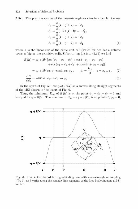
422 Solutions of Selected Problems
5.5s. The position vectors of the nearest-neighbor sites in a bcc lattice are:
1 =a
2(i + j + k) = −
′1 ,
2 =a
2(−i + j + k) = −
′2 ,
3 =a
2(i − j + k) = −
′3 ,
4 =a
2(i + j − k) = −
′4 , (1)
where a is the linear size of the cubic unit cell (which for bcc has a volumetwice as big as the primitive cell). Substituting (1) into (5.15) we find
E (k) = ε0 + 2V [cos (φ1 + φ2 + φ3) + cos (−φ1 + φ2 + φ3)+ cos (φ1 − φ2 + φ3) + cos (φ1 + φ2 − φ3)]
= ε0 + 8V cosφ1 cosφ2 cosφ3 , φi =kia
2, i = x, y, z , (2)
∂E
∂φi= −8V sin φi cosφj cosφk . (3)
In the spirit of Fig. 5.3, we plot E (k) as k moves along straight segmentsof the 1BZ shown in the insert of Fig. 6.
Thus, the minimum, Em, of E (k) is at the point φ1 = φ2 = φ3 = 0 andis equal to ε0 − 8 |V |. The maximum, Em = ε0 + 8 |V |, is at point H , φ1 = 0,
ε0 − 8|V |
ε0
ε0 + 8|V |
ΓNHPNΓ
E(k
)
ε0 − 8|V |
ε0
ε0 + 8|V |
ΓNHPNΓ
E(k
)
ε0 − 8|V |
ε0
ε0 + 8|V |
ΓNHPNΓ
E(k
)
ε0 − 8|V |
ε0
ε0 + 8|V |
ΓNHPNΓ
E(k
)
ε0 − 8|V |
ε0
ε0 + 8|V |
ΓNHPNΓ
E(k
)
ε0 − 8|V |
ε0
ε0 + 8|V |
ΓNHPNΓ
E(k
)
ε0 − 8|V |
ε0
ε0 + 8|V |
ΓNHPNΓ
E(k
)
ε0 − 8|V |
ε0
ε0 + 8|V |
ΓNHPNΓ
E(k
)
ε0 − 8|V |
ε0
ε0 + 8|V |
ΓNHPNΓ
E(k
)
ε0 − 8|V |
ε0
ε0 + 8|V |
ΓNHPNΓ
E(k
)
ε0 − 8|V |
ε0
ε0 + 8|V |
ΓNHPNΓ
E(k
)
ε0 − 8|V |
ε0
ε0 + 8|V |
ΓNHPNΓ
E(k
)
ε0 − 8|V |
ε0
ε0 + 8|V |
ΓNHPNΓ
E(k
)
ε0 − 8|V |
ε0
ε0 + 8|V |
ΓNHPNΓ
E(k
)
kxky
kz
HD
NG
PΔ
ΛΓ
Σ
N: 2
P: 2
Fig. 6. E vs. k for the 3-d bcc tight-binding case with nearest-neighbor couplingV (< 0), as k varies along the straight-line segments of the first Brillouin zone (1BZ)for bcc

Solutions of Selected Problems 423
φ2 = π, φ3 = 0 (plus two others resulting from cyclic permutations). Alongthe line segment PNP′ (φ1 = π/2, φ2 = π/2, −π/2 ≤ φ3 ≤ π/2) (plus 11 moreresulting from cyclic permutations and changing the signs to ±π/2) E(k) = ε0
and ∂E/∂φi = 0 for all i = x, y, z. Hence the DOS must exhibit a logarithmicsingularity at E = ε0 and be of the form depicted in Fig. 7.
The position vectors for nearest neighbors in an fcc lattice are:
1± =a
2(i ± j) = −′1± ,
2± =a
2(j ± k) = −′2± ,
3± =a
2(k ± i) = −′3± .
Substituting (4) into (5.15) we find after some algebra
E = ε0 − 4 |V | (cosφ1 cosφ2 + cosφ2 cosφ3 + cosφ3 cosφ1) , (4)
where φi = kia/2 and a is the linear size of the cubic unit cell (which for fcchas a volume four times the volume of the primitive cell).
In Fig. 8 we plot E vs. k in the spirit of Fig. 5.3.Thus the minimum value, Em = ε0 − 12 |V |, of E (k) is obtained at the
point Γ (φ1 = φ2 = φ3 = 0) and the maximum, EM , along line segment XW(−π/2 ≤ φ1 ≤ π/2, φ2 = π, φ3 = 0) and five more resulting from symmetryconsiderations. The derivatives
∂E
∂φi= 4 |V | sin φi (cosφj + cosφk) , i = j = k = i , for all i
indeed vanish along XW (and symmetric lines) as well as on the isolated pointL (and points symmetric to it). Point L is a saddle point with two positive As
ε0ε0 − 8 |V | ε0 + 8 |V |
E
DOS
Fig. 7. Schematic plot of DOS for bcc TBM (see text)

424 Solutions of Selected Problems
ε0 − 12|V |
ε0
ε0 + 4|V |
XU≡KΓLWXΓ
E(k
)
ε0 − 12|V |
ε0
ε0 + 4|V |
XU≡KΓLWXΓ
E(k
)
ε0 − 12|V |
ε0
ε0 + 4|V |
XU≡KΓLWXΓ
E(k
)
ε0 − 12|V |
ε0
ε0 + 4|V |
XU≡KΓLWXΓ
E(k
)
ε0 − 12|V |
ε0
ε0 + 4|V |
XU≡KΓLWXΓ
E(k
)
ε0 − 12|V |
ε0
ε0 + 4|V |
XU≡KΓLWXΓ
E(k
)
ε0 − 12|V |
ε0
ε0 + 4|V |
XU≡KΓLWXΓ
E(k
)
ε0 − 12|V |
ε0
ε0 + 4|V |
XU≡KΓLWXΓ
E(k
)
ε0 − 12|V |
ε0
ε0 + 4|V |
XU≡KΓLWXΓ
E(k
)
ε0 − 12|V |
ε0
ε0 + 4|V |
XU≡KΓLWXΓ
E(k
)
ε0 − 12|V |
ε0
ε0 + 4|V |
XU≡KΓLWXΓ
E(k
)
ε0 − 12|V |
ε0
ε0 + 4|V |
XU≡KΓLWXΓ
E(k
)
ε0 − 12|V |
ε0
ε0 + 4|V |
XU≡KΓLWXΓ
E(k
)
ε0 − 12|V |
ε0
ε0 + 4|V |
XU≡KΓLWXΓ
E(k
)
ε0 − 12|V |
ε0
ε0 + 4|V |
XU≡KΓLWXΓ
E(k
)
Fig. 8. E vs. k for 3-d fcc tight-binding case with nearest-neighbor coupling V (< 0),as k varies along straight-line segments of first Brillouin zone (1BZ) for fcc
along directions perpendicular to (1, 1, 1) and one negative along the direction(1, 1, 1). Thus the DOS for the fcc resembles that in the sketch in Fig. 9. 5.7s. Let us call G1, G1, and G2 the quantities G(1, 1), G(1, 1[2]), andG(2, 2[1]), respectively. Combining (F.10) and (F.11) we have
1G1
= z − ε1 − ∆ = z − ε1 − (K + 1)V 2G2 . (1)
From (F.12) and (F.13) we find
fcc
Eε0 + 4 |V |ε0 − 12 |V | ε0
DOS
Fig. 9. Schematic plot of DOS for fcc TBM (see text)

Solutions of Selected Problems 425
1G1
= z − ε1 − KV 2G2 . (2)
We multiply (1) by K and (2) by K + 1, and we subtract
K + 1G1
− K
G1= (K + 1) (z − ε1) − K (z − ε1) = z − ε1 ,
orG1 =
K + 1z − ε1 + KG−1
1
. (3)
Chapter 6
6.3s.
0
0.5
1
1.5
2
2.5
3
3.5
-1 -0.5 0 0.5 1
(E
)
E
ε/B−0.6−0.8−0.9
Fig. 10. Plot of DOS for simple cubic TBM at site of impurity
426 Solutions of Selected Problems
6.4s. We start from (6.25). The quantity⟨n∣∣G+
0
∣∣ ⟩, according to (5.28), isgiven by ⟨
n∣∣G+
0
∣∣ ⟩ = G+0 (, )||1 , (1)
where
1 = −z − ε0
B+ i
√1 −
(z − ε0
B
)2
= cos(ka) + i√
1 − cos2(ka)= cos(ka) + i sin(ka) = eik (2)
sincez = E(k) = ε0 − B cos(ka) . (3)
We then have, by substituting (2) into (6.25),
〈n|ψE) = 〈n|k) +εG+(, ; E)eik|−n|eik
√N[1 − εG+
0 (, ; E)] . (4)
• For n > , i.e., for transmission, we have
√N 〈n|ψE) = eikn +
εG+0 (, ; E)
1 − εG+0 (, ; E)
eikn
=1
1 − εG+0 (, ; E)
eikn, n > . (5)
• For n < , i.e., for reflection, we have
√N 〈n|ψE) = eikn +
εG+0 (, ; E)e2ike−ikn
1 − εG+0 (, ; E)
= eikn + e−ikne2ik εG+0 (, ; E)
1 − εG+0 (, ; E)
(6)
=1
e−ik
×[eik(n−) + e−ik(n−) εG+
0 (, ; E)1 − εG+
0 (, ; E)
], n < . (7)
Thust =
11 − εG+
0 (, ; E)(8)
and
r =εG+
0 (, ; E)1 − εG+
0 (, ; E). (9)

Solutions of Selected Problems 427
−1.118
−0.5
0.5 ε/B0
0.5
1.118
E/B
−0.5
Fig. 11. Plot of the bound states eigenenergy(ies) vs. the local perturbation fora two-band (shaded areas) model shown in Fig. 5.12
6.5s. Schematic plot of the bound-state eigenenergies, Ep, vs. the localperturbation |1〉 ε 〈1| for the double spacing periodic Cayley tree with K = 3,ε1 = −ε2 = B/2. The upper and lower edges of the two subbands are alsoshown. Notice that for ε < −0.539B there are two bound eigenenergies (onein the gap and the other below the lower band); for 0 < ε < 0.206B there isno bound state; finally, for 0.206B < ε there is only one bound state abovethe upper band. 6.6s. We introduce the center of mass, K, and the relative, k, by the relationsK = k1 + k2 and k = (k1 − k2) /2 so that
k1 =12K + k , (1a)
k2 =12K − k . (1b)
We have the inequalities
k21 =
K2
4+ k2 + K ·k > k2
F , (2a)
k22 =
K2
4+ k2 − K ·k > k2
F . (2b)
Furthermore,
E =
2
2m
(k21 + k2
2
)=
2
m
(K2
4+ k2
)(3)
or

428 Solutions of Selected Problems
k =
√mE
2− K2
4. (4)
From (2a) and (2b) in combination with (3) we have
−(
mE
2− k2
F
)< K ·k <
mE
2− k2
F , (5)
which, in view of (4), becomes
|cos θ| <mE2 − k2
F
K√
mE2 − K2
4
. (6)
The DOS per unit volume, (E; K), equals (2π)−3dΩk/dE, where dΩk is theelementary available volume in phase space between E and E + dE. Thus
(E; K) =1
(2π)3
∫dφdθ sin θk2dk
δ
(k −
√mE2 − K2
4
)dE
× θ (E − 2EF ) , (7)
where, according to (3), dE/dk = 22k/m. If we denote by A the maximum
value of |cos θ| [taking into account (6)] and perform the integrations in (7),we find
0(E; K) =A
4π2
m
2
√mE
2− K2
4θ (E − 2EF ) , (8)
where
A = min
⎡⎣1,mE2 − k2
F
K√
mE2 − K2
4
⎤⎦ . (8′)
For K = 0 we obtain
0(E; 0) =1
4π2
(m
2
)3/2 √Eθ (E − 2EF )
=1
2√
2π2
(m
2
)3/2√
E
2θ (E − 2EF )
=12
(E
2
)θ (E − 2EF ) , (9)
where (E) is the DOS for a single free particle of mass m. For K = 0,E → 2EF , and taking into account (3), we have for the quantity A
A → E − 2EF
2Kk/m,
and consequently
0(E; K) → 14π2
(m
2
)2 E − 2EF
Kθ (E − 2EF ) , K = 0, E → 2EF .
(10)

Solutions of Selected Problems 429
6.7s. The DOS is given by
0(E) = F12
[1 − 2f
(E
2
)]=
F
2eβ(E/2−EF ) − 1eβ(E/2−EF ) + 1
=F
2tanhx , (1)
where x ≡ β2
(E2 − EF
)and dE = 4
β dx and the integration limits are x =−βωD/2 and βωD/2. Thus we have for G0(E)
G0(z) =∫ βωD/2
−βωD/2
dxF
24β
tanhx
z − (4x/β) − 2EF, (2)
and the value of G0(z) for z = 2EF is
G0 (2EF ) = −F
2
∫ βωD/2
−βωD/2
dx tanhx
x= −F
∫ βωD/2
0
dx tanhx
x. (3)
Integrating by parts we have
G0 (2EF ) = −F
(lnx tanh x|βωD/2
0 −∫ βωD/2
0
dxlnx
cosh2 x
)
= −F
(ln
βωD
2tanh
βωD
2−∫ βωD/2
0
dx lnx
cosh2 x
). (4)
In the limit βωD 2 or kBT ωD/2 we have approximately
G0 (2EF ) = −F
(ln
βωD
2−∫ ∞
0
dxlnx
cosh2 x
). (5)
The integral in (5) equals lnπ−ln 4−γ, where γ = 0.577215 . . . is the so-calledEuler’s constant. We can write (5) as follows:
G0 (2EF ) = −F ln2eγ
ωD
πkBT, kBT ωD . (6)
Chapter 7
7.1s. Following a procedure similar to that of Problem 6.4s (and takinginto account that 1 = eika = eiφ) we obtain the following expressions for thetransmission, t, and the reflection, r, amplitudes:
t = 1 + G0Tf , (1a)r = G0Tb , (1b)

430 Solutions of Selected Problems
where G0 is the diagonal matrix element of the unperturbed Green’s functionG0 = G0(, ), and Tf and Tb are the forward and backward matrix elementsof T , respectively, given by
Tf = T + Tmm + Tmeika + Tme−ika , (2a)
Tb = e2ikaT + e2ikamTmm + eika(+m)Tm + eika(+m)Tm . (2b)
More generally, if we have impurities at the sites 1,. . . ,p (which are notnecessarily consecutive), the expressions for Tf and Tb are
Tf =∑ij
exp [ika (i − j)] 〈j |T | i〉 , (3a)
Tb =∑ij
exp [ika (i + j)] 〈j |T | i〉 . (3b)
The matrix elements T, Tmm, Tm, Tm in (2a) and (2b) are given by em-ploying (7.12) and (7.13). The result is the following:
Tf = fm [t + tm + 2ttmG0(, m) cos(ka)] (4a)= fm
[t + tm + 2ttmG0eika cos(ka)
], (4b)
where G0 ≡ Go(, ) and
fm =[1 − ttmG2
0e2ika
]−1. (5)
The reader may calculate numerically and plot |t|2 = |1 + G0Tf |2 vs. x ≡E/B = − cos(ka) for various values of ε and ε′ (especially for those close tothe boundaries in Fig. 7.3a). 7.2s. In matrix notation the unperturbed Hamiltonian, H0, satisfies therelations
〈 |H0 | 〉 =∣∣∣∣ εs 00 εp
∣∣∣∣ , (1)
〈 |H0 | ± 1〉 =∣∣∣∣Vss ±Vsp
∓Vsp Vpp
∣∣∣∣ =∣∣∣∣V2 ±V ′′
2
∓V ′′2 V ′
2
∣∣∣∣ . (2)
We define the matrix state |k) = [|ks) , |kp)] by
|k) =1√N
∑
eika |〉 . (3)
The |k) states are orthonormal in the sense that
(k|k′) = δkk′1 , (4)
where 1 is the 2 × 2 unit matrix.

Solutions of Selected Problems 431
Let us calculate the matrix elements of H0 in the |k) basis
(k| H0 |k′) =1N
∑m
eik′ma−ika 〈 | H0 |m〉 =
=1N
∑m
[ei(k′−k)ma
∣∣∣∣ εs 00 εp
∣∣∣∣+ ei(k′−k)mae−ika
∣∣∣∣V2 −V ′′2
V ′′2 V ′
2
∣∣∣∣+ ei(k′−k)maeika
∣∣∣∣V2 V ′′2
−V ′′2 V ′
2
∣∣∣∣] ,
or (taking into account that∑
m ei(k′−k)ma = Nδkk′ )
(k| H0 |k′) = δkk′
∣∣∣∣ εs + 2V2 cos(ka) 2iV ′′2 sin(ka)
−2iV ′′2 sin(ka) εp + 2V ′
2 cos(ka)
∣∣∣∣ . (5)
Now the matrix elements of the Green’s function G0 in the initial |〉 basisis ⟨
∣∣ (z −H0)−1
∣∣m⟩=∑kk′
〈|k) (k| (z −H0)−1 |k′) (k′|m〉
=1N
∑k
eik(−m)a [z1− E2(k)]−1, (6)
where E2(k) is the matrix in (5) and 1 is the unit 2× 2 matrix. Thus we haveto find the inverse of the matrix
z1− E2(k) =∣∣∣∣ z − εs − 2V2 cos(ka) −2iV ′′
2 sin(ka)2iV ′′
2 sin(ka) z − εp − 2V ′2 cos(ka)
∣∣∣∣ . (7)
We have
[z1− E2(k)]−1 =1
D(k)
∣∣∣∣ z − εp − 2V ′2 cosφ 2iV ′′
2 sin φ−2iV ′′
2 sinφ z − εs − 2V2 cosφ
∣∣∣∣ , (8)
where φ = ka and
D(k) = (z − εs − 2V2 cosφ) (z − εp − 2V ′2 cosφ) − 4V ′′
22 sin2 φ .
The summation over k from −π/a to π/a and the division by N would betransformed to an integration over φ from −π to π (over 2π). The off-diagonalmatrix elements in (8) are odd functions of k or φ, and consequently the = mmatrix element would be diagonal:
(| (z −H0)−1 |) =
∣∣∣∣G0ss(z) 00 G0pp(z)
∣∣∣∣ , (9)
where
G0ss(z) =∫ π
−π
dφ
2π
z − εp − 2V ′2 cosφ
D(φ), (9a)
G0pp(z) =∫ π
−π
dφ
2π
z − εs − 2V2 cosφ
D(φ). (9b)

432 Solutions of Selected Problems
The perturbing Hamiltonian corresponding to the impurity at the n-site,|n〉 ε′ 〈n|, where ε′ is a 2 × 2 diagonal matrix with ε′s and ε′p, shall modifythe Green’s function as in (6.8) and (6.10):
G(, m) − G0(, m) = G0(, n)ε′ [1 − G0(n, n)ε′]−1G0(n, m)
= G0(, n) [1 − ε′G0(n, n)]−1ε′G0(n, m) , (10)
where G0(n, n) is a 2× 2 matrix given by (9), (9a), and (9b). Since in generalboth ε′ and G0(, m) are matrices, the ordering is important [not in the presentcase since the matrices ε′ and G0(n, n) are both diagonal]. We have for them
[1 − ε′G0(n, n)]−1 = [1 − G0(n, n)ε′]−1
=
∣∣∣∣∣ [1 − ε′sG0ss]−1 0
0[1 − ε′pG0pp
]−1
∣∣∣∣∣ . (11)
Thus, the bound states would appear as solutions to the equations
1ε′s
= G0ss(E) , (12a)
1ε′p
= G0pp(E) . (12b)
In particular, for a vacancy (for which ε′s = ε′p = ∞) we have
G0ss(E) = 0 , (13a)G0pp(E) = 0 . (13b)
The reader may calculate G0ss(E) and G0pp(E) numerically for εs, εp, V2, V ′2 ,
and V ′′2 appropriate for Si as given in Problem 5.6. He can compare his result
with those of a more realistic model for Si in [52]. 7.5s. We introduce the dimensionless quantities z = E/B, σ = Σ+/B,a = ε/B, and g = BG+ = BG+
0 (E − Σ+). Then (7.59a) becomes
σ =12
[a
1 − (a − σ)g− a
1 + (a + σ)g
], (1)
where for the Hubbard Green’s function we have
g = 2(z − σ −
√(z − σ)2 − 1
). (2)
Keep in mind that Im z → 0+, Im σ ≤ 0, Im g ≤ 0.Iterate (1) for each value of a and z until you obtain convergence, which
is facilitated by starting with a nonnegligible value of Im z and large valuesof Re z (Re z = 1 + a). Sometimes, convergence is accelerated if, in eachstep n, you employ as a starting value of σ half the sum of the input plus theoutput value of σ.

Solutions of Selected Problems 433
The results are shown in Fig. 12. Note that as ε is increasing, a deepdevelops at the center of the band that becomes deeper and deeper, andeventually the band splits into two subbands separated by a gap. 7.6s. The CPA obtains Σ from (7.59a), which can be recast as
Σ(E) =∫
dεp(ε)ε
1 − (ε − Σ)G, G = 〈n |G0 (E − Σ) |n〉 . (1)
We shall examine the case of weak disorder, i.e., (w/ |V |) ≤ 1, and we shalldistinguish two subcases (a) |ε| ≤ w, (b) |ε| w, where w is the standarddeviation of the Gaussian probability function, p(ε).
In subcase (a) we can expand the denominator in (1) in powers of (ε − Σ)Gand keep terms up to third order. We find
Σ w2G − (2w4 − µ4
)G3 + O
(w6
), (2)
where µ4 ≡ ⟨ε4⟩
= 3w4.In subcase (b), the main contribution to the integral in (1) comes from
the pole of the denominator. Thus
Σ −iπ
G20(E)
p(G−1
0
), (3)
since |Σ| |ε| in this case. Hence, in subcase (b) the DOS per unit volume is
(E) =1ad
G′0(E)
G20(E)
p(G−1
0 (E))
. (4)
0
0.1
0.2
0.3
0.4
0.5
0.6
0.7
-2 -1.5 -1 -0.5 0 0.5 1 1.5 2
=
−1 πIm
g(E
)
E/B
ε/B0.20.40.60.81.0
Fig. 12. Density of states for a random binary alloy AxB1−x (x = 0.5) with εA +εB = 0 and εA − εB = 2ε. The unperturbed bandwidth is 2B; B has been taken asthe unit of energy

434 Solutions of Selected Problems
The reader may verify, by using Table 5.2, that for a simple cubic lattice
G−20 (E) 18.6V 2 − 15.76 |V |E , 3V ≤ E ≤ 0.1V , (5)
where E = 0 coincides with the unperturbed lower band edge, and V < 0.Substituting (5) into (4) we obtain the DOS at the tail, which over the
range shown in (5) is exponential in E
tail ∼ exp(−|E|
E0
), E0 =
w2
7.88 |V | . (6)
This exponential tailing in the DOS leads to exponential subgap optical ab-sorption in crystalline and amorphous semiconductors (Urbach tails) withan E0 of the form E0 = E0s + E0T , where E0s is due to static disorder andE0T ∼ kBT is due to thermal disorder.
Returning now to subcase (a) and taking into account that G0(E) =G0(0) + α
√−E as E → 0− with α = 1/4π |V |3/2 and G0(0) = −0.2527/ |V |,we have from (2)
Σ = w2G0(0) + αw2√
Σ − E + w4G30(0) . (7)
This is a quadratic equation for Σ. The CPA band “edge,” ECPA, is deter-mined when Im Σ = 0, where Σ is the solution of (7). This condition leadsto
ECPA = G0(0)w2 +[α2
4+ G3
0(0)]
w4
= −0.2527w2
|V | +[
164π2
− (0.2527)3]
w4
|V |3 . (8)
The quantity w2G0(0)+w4G30(0) in (7) can be replaced by ECPA−(
α2w4/4),
in view of (8), so that (7) becomes
Σ − E = αw2√
Σ − E − (E − ECPA) − α2w4
4. (9)
By introducing the unit of energy
ε0 =α2w4
4=
w4
4(4π)2 |V |3 ,
(9) is reduced to a dimensionless universal form
Σ − E = 2√
Σ − E − x − 1 , (10)
where Σ = Σ/ε0, E = E/ε0, and x = (E − ECPA) /ε0. The solution of (10)is Σ − E = 1 − x + 2
√−x.

Solutions of Selected Problems 435
7.9s. We introduce the notation
q0 = ω/c0 , c0 =√
B0/0 , c =√
B/ ,q = ω/c , ∆ = 0/ , M = c0/c .
The incident wave, φi, is
φi = exp (iq0z) =∞∑
=0
i(2 + 1)j (q0r) P(cos θ) . (1)
The scattered wave, φs, and the wave inside the sphere, φins, are of the form
φs = −∞∑
=0
i(2 + 1)rh (q0r) P(cos θ) , h ≡ h(1) , (2a)
φins =∞∑
=0
i(2 + 1)Ij(qr)P(cos θ) . (2b)
The coefficients r and I are determined from the BC
j0 − r0h0 =1∆
Ij , (3a)
q0j′0 − rq0h
′0 = Iqj
′ , (3b)
where the argument of j0 and h0 is q0a, while that of j is qa; prime denotesdifferentiation with respect to q0r or qr.
The result for r is
r =j′0j − xj0j
′
h′0j − xh0j′
, x =q0
q0. (4)
The equation for the energy flux can be written
j = − 20
B0 + B∗0
ReB∗
0 φ∇φ∗
. (5)
Substituting φ = φi + φs into (5) we find that
j = ji + js + jis , (6)
wherejis = − 20
B0 + B∗0
Re
B∗φi∇φ∗s + B∗φs∇φ∗
i
. (7)
From energy conservation, ∫r≤a
d3r∇· j + Q = 0 ,

436 Solutions of Selected Problems
where Q is the energy dissipation within the sphere; taking into account (6),we have
−∫
jis · dS =∫
ji · dS +∫
js · dS + Q . (8)
The first integral on the rhs of (8) is zero, the second one gives the scatteringcross section (times |ji|), while Q gives the absorption cross section (due todissipation inside the sphere) times |ji|. Thus, the total cross section (TCS),which is also called the extinction cross section, is given by minus the integralof jis over the surface of the sphere divided by |ji|.
Performing the integral of jis over the surface of the sphere we find, aftera lengthy but straightforward calculation, that
TCS = 4πIm C
Re B0q0 , (9)
where
C = B0q0a2
∞∑=0
(2 + 1) (j∗0h′0r + j′0h
∗0r
∗ ) , (10)
and the subscript zero indicates that the argument of the Bessel and theHankel functions is q0a.
It is left to the reader to show that in the absence of losses in the hostmaterial (i.e., when Im B0 = 0), (9) and (10) reduce to the usual formulaefor the total scattering section
TCS =4π
q0Im f(0) =
4π
q20
∞∑=0
(2 + 1)Re r . (11)
8.1s. In the presence of an electric potential φ, the chemical potential, µ,becomes
µ = µ0 + qφ , (1)
where µ0 is its expression in the absence of φ and q is the charge of eachparticle. Equilibrium demands that µ must be a constant throughout thesystem. If this is not the case, a particle current is set up proportional to−∇µ (for not-so-large values of |∇µ|):
jp = −c∇µ = −cδµ0
δn∇n − cq∇φ . (2)
By definition, the diffusion coefficient is the coefficient of −∇n:
D = cδµ0
δn; (3)
the coefficient of −∇φ = E is by definition the conductivity divided by q:
σ = cq2 . (4)
Solutions of Selected Problems 437
Substituting the linear coefficient c from (3) into (4) we have
σ = q2Dδn
δµ0. (5)
By making explicit the spatial nonlocal dependencies of σ, D, and δn/δµ0 weobtain (8.10).
For kBT EF the relation
n =∫
dε(ε)1
eβ(ε−µ) + 1
reduces ton =
∫dε(ε)e−β(ε−µ) .
Hence∂n
∂µ= βn ,
from which (8.11b) follows. 9.1s. The conductance, G, of a wire of cross section A and length L is givenby
G =σA
L, (1)
where σ is the conductivity of the material in the limits L → ∞ and A =L2 → ∞.
Generalizing (9.42) and (9.43) to a wire we have
G =e2
2π
cλA
L− e2
2π, (2)
where in the place of ξ (the localization length of a 1-d system) we havesubstituted cλA; λA is the localization length of the wire given by λA =A/4.82ξ′ and c is a numerical factor which, by the method of §9.6.1, turns outto be about 2. Combining (1) and (2) and the expression for λA we obtain
σ =c
4.82 × 2π
e2
1ξ′
for L → ∞ . (3)
When L−1 > 0 we have to add to (3) a term proportional to L−1, which,according to (9.2c), is equal to
12√
2π2
e2
1LM
=√
c1
2√
2π2
e2
1L
. (4)
In (4) we took into account (9.5) and assumed that L−1φ = L−1
ω = L−1β = 0.
Combining (3) and (4) we obtain
σ =e2
(0.066
ξ′+
0.036√
c1
L
). (5)

438 Solutions of Selected Problems
According to the potential well analogy, ξ′ blows up at a critical value(S2
tr
)c
[see (9.30)] with a critical exponent s = 1 (keep in mind that the correctcritical exponent is larger, s 1.54). Thus
ξ′ =C
S2tr − (S2
tr)c
;
from (9.2c), the critical value turns out to be 12c′1, where c′1 = tr/Lm. Thequantity C is determined by going to the weak scattering case, where S2
tr (S2
tr
)c
and σ =(e2/12π3
)Str. Equating this value of σ with the value
0.066e2/ξ′, where ξ′ = C/S2tr, we find
C = 12π3 × 0.066 24.56 .
9.5s. We shall employ (9.106a) and (9.106b) [for a discrete system √
vpvq
must be divided by the lattice spacing a as in (9.111)]. The Green’s functionwill be calculated by the same trick as in Problem 9.9 below, i.e., we shallintroduce a 2 × 2 Hamiltonian of the form
H ≡( H0 H01
H01 H1
), (1)
where H0 describes an infinite periodic 1-d TBM, H1 a semi-infinite periodicTBM terminated at point 1d (i.e., the perpendicular leg of T ) and H01 =V ′ (|0〉 〈1d| + |1d〉 〈0|). Corresponding to H is a 2 × 2 Green’s function thatsatisfies the matrix equation(
E −H0 −H01
−H01 E −H1
)( G0 G01
G10 G1
)=(
1 00 1
). (2)
More explicitly, (2) is equivalent to the following four equations:
(E −H0)G0 −H01G10 = 1 , (2a)−H01G0 + (E −H1)G10 = 0 , (2b)−H01G1 + (E −H0)G01 = 0 , (2c)
(E −H1)G1 −H01G01 = 1 . (2d)
Combining (2a) and (2b) we obtain
G0 = G0 + G0H01G1H01G0 , (3)
whereG0 = (E −H0)
−1 and G1 = (E −H1)−1
. (4)
Similarly, from (2c) and (2d) we have
G1 = G1 + G1H01G0H01G1 . (5)

Solutions of Selected Problems 439
Let us calculate first 〈0 | G0 |m〉 = G0(0, m) from (3):
G0(0, m) = G0(0, m) + G0(0, 0)V ′G1 (1d, 1d)V ′G0(0, m) , (6)
orG0(0, m) =
G0(0, m)1 − V ′2G0(0, 0)G1 (1d, 1d)
. (6′)
We remind the reader that
G0(n, m) =−i
2 |V | sin φei|n−m|φ , φ = ka . (7)
From (3), (6′), and (7) we can easily show that
G0(n, m) = G0(n, m) + G0(n, 0)G1 (1d, 1d) V ′2G0(0, m) . (8)
To find the current transmission amplitude from left to right we have from(9.106a)
tr = ive−iφ(|n|+|m|)G0(n, m)a
. (9)
Taking into account that v = −2V a sinφ, and substituting in (9) from (8),(7), and (6′) we obtain
tr =[1 + i
V ′2
2 |V | sin φG1 (1d, 1d)
]−1
. (10)
It remains to calculate G1 (1d, 1d); this corresponds to a Hamiltonian wheresite 0 is a vacancy. Hence
G1 = G0 − G0|0〉 〈0|
G0 (1d, 1d)G0
or
G1 (1d, 1d) = G0 (1d, 1d) − G0 (1d, 1d) e2iφ =−i
2 |V | sin φ
(1 − e2iφ
). (11)
Substituting in (10) we have
tr =(
1 +V ′2
V 2
1 − e2iφ
4 sin2 φ
)−1
=1 − e−2iφ
1 + x2 − e−2iφ, x2 =
V ′2
V 2. (12)
The reader may obtain the remaining matrix elements of s by the same ap-proach. 9.6s. Because of the one-parameter scaling assumption we have that
Q = f (L/ξ′) , (1)

440 Solutions of Selected Problems
where ξ′ is a function of Q such that ξ′ = c (Q − Qc)−s, as Q → Q+
c . Differ-entiating this last relation we have
d
dQ
(1ξ′
)=
s
c(Q − Qc)
s−1. (2)
By definition of β we obtain from (1)
β =L
Q
dQ
dL=
L
Qf
1ξ′
, (3)
where the dot over f denotes differentiation with respect to the argumentL/ξ′. Now, using the relation
ddQ
(L
ξ′
)=[
dQ
d (L/ξ′)
]−1
=1f
, (4)
and keeping L constant, we have that
ddQ
(1ξ′
)=
1L
1f
=1L
L
Q
1ξ′
1β
=1
Qξ′β. (5)
In (5) we have replaced f from (3). Substituting in (5) ξ′ by c (Q − Qc)−s,
d (1/ξ′) /dQ from (2), and setting β = (dβ/dQ)c (Q − Qc) as Q → Qc [sinceby definition β (Qc) = 0], we find that
s =1
Qc (dβ/dQ)c
. (6)
9.7s. We have from (9.72)
ξ−1 =12
∫ ∞
−∞dεp(ε)
∫ ∞
−∞dxf0(x) ln
∣∣∣1 +ε
x
∣∣∣=
14
∫ ∞
−∞dεp(ε)
∫ ∞
−∞dxf0(x) ln
∣∣∣∣1 − ε2
x2
∣∣∣∣=
12
∫ ∞
−∞dεp(ε)
∫ ∞
0
dxf0(x) ln∣∣∣∣1 − ε2
x2
∣∣∣∣ . (1)
Taking into account that f0(x) = C/√
1 + x4, we have for the integral
I ≡∫ ∞
0
dx1√
1 + x4ln∣∣∣∣1 − ε2
x2
∣∣∣∣=∫ ∞
0
dx
(1√
1 + x4− 1
)ln∣∣∣∣1 − ε2
x2
∣∣∣∣ , (2)
since ∫ µ
0
dx ln∣∣∣∣1 − ε2
x2
∣∣∣∣ −→µ→∞
ε2
µ→ 0 . (3)

Solutions of Selected Problems 441
We split integral (2) from 0 to ε and from ε to ∞. In the first integral wewrite
1√1 + x4
≈ 1 − 12x4
since ε → 0, while in the second we expand the logarithm
ln∣∣∣∣1 − ε2
x2
∣∣∣∣ = −∞∑
n=1
1n
( ε
x
)2n
. (4)
ThusI = I1 + I2 ,
where
I1 =∫ ε
0
dx
(−x4
2
)ln∣∣∣∣1 − ε2
x2
∣∣∣∣ → O(ε5)
for ε → 0 , (5)
I2 =∞∑
n=1
ε2n
n
∫ ∞
ε
dx
(1 − 1√
1 + x4
)1
x2n. (6)
Each term in the series (6) is of order higher than ε2, except for the n = 1,for which we have
I(1)2 = ε2
∫ ∞
ε
(1 − 1√
1 + x4
)1x2
. (7)
This integral can be expressed in terms of elliptic functions (see [11], p. 261):
I(1)2 = −ε2
2[F(α, r) − 2E(α, r)] + O
(ε3)
, (8)
where
α = arccos(
ε2 − 1ε2 + 1
)→ π as ε → 0 ,
r =1√2
.
ButF(π, r) = 2K(r) and E(π, r) ≡ 2E(r) . (9)
Thus finally
I = I(1)2 + O
(ε3)
= −ε2 [K(r) − 2E(r)] + O(ε3)
. (10)
Hence the inverse localization length to order σ2 is given by
ξ−1 =C
2
∫ ∞
−∞dεp(ε)I(1)
2 , where C =1
2K(r)(11)

442 Solutions of Selected Problems
according to (9.77). Thus finally
ξ−1 =2E(r) −K(r)
4K(r)σ2 ,
where σ is the standard deviation of p(ε). 9.10s. From (8.75) we have
s 〈G (0, 0; E + is)G (0, 0; E − is)〉 =s
N
∑q
A (q)1 − uA (q)
, (1)
where, according to (8.82),
u (z, z′)A (q; z, z′) → 1 + a1 (z − z′) − a2q2 (2)
as z → z′ and q → 0; a1 = i/2 |Σ2| and a2 = D(0)/2 |Σ2| according to (8.83)and (8.85), respectively. In the present case, z − z′ = 2is.
Substituting in (1) we have
s⟨G+G−⟩ = c
s
N
Ω
(2π)d
∫dq
(1/u) |Σ2|s +
(D(0)/2
)q2
=c
(2π)d
Ω
Ns
∫dq
π′
s + (D0/2) q2, (3)
where we have taken into account that u = |Σ2| /π′ and we have introduceda numerical factor c to correct for the fact that expansion (2) is valid for smallvalues of q.
For d = 3 the q2 term in the denominator (in the limit s → 0+) is cancelledby a q2 phase space factor in the numerator (coming from dq ∼ q2dq), andhence (3) approaches zero linearly in s, indicating thus the validity of theperturbation expansion. In contrast, for d = 2 or d = 1 the phase spacefactor is q or 1, respectively, and the integral blows up. Although the integralblows up as s → 0, the quantity s 〈G+G−〉 still approaches zero: as
√s/D(0)
in one dimension and as(s/D(0)
)ln∣∣s/D(0)
∣∣ in two dimensions. If thisresult is accepted, one must conclude that the eigenstates are neither extendednor normalizable; instead, they decay very slowly to zero. However, we knowthat, at least in one dimension, the states are exponentially localized. Hence,we must conclude that the singularities of the vertex part obtained throughthe CPA or the post-CPA, although indicative of localization effects, are notcapable of fully describing the situation at all length scales. It is assumedthat at short length scales, when one does not sample the extreme tails of theeigenfunctions, the CPA and the post-CPA vertex corrections are satisfactory.
One way of improving the present method is to replace in (3) D(0) by D,the corrected diffusion coefficient, which in general is ω and q dependent. SinceD(ω) is proportional to iω, then s 〈G+G−〉 goes to a nonzero limit as ω → 0first and then s → 0+, and thus regular localization is recovered.

Solutions of Selected Problems 443
10.6s. Since the particles do not interact, their Hamiltonian has the form
H =∑
i
εia†iai . (1)
The quantity⟨a†
iai
⟩to be calculated is by definition
⟨a†
iai
⟩=
Tra†
iaie−β(H−µN)
Tre−β(H−µN)
. (2)
We have thatai exp
(−xa†
iai
)= e−x exp
(−xa†
iai
)ai . (3)
Equation (3) can be proved by acting on any eigenfunction of a†iai (a†
iai |φ〉 =
ni |φ〉) and taking into account that f(a†
iai
)ai |φ〉 = f (ni − 1) ai |φ〉. Then
we writeH− µN = (εi − µ) a†
iai +∑j =i
(εj − µ) a†jaj ,
and we have
Tra†
iaie−β(H−µN)
= Tr
⎧⎨⎩a†iai exp
[−β (εi − µ) a†
iai
]exp
⎡⎣−β∑j =i
(εj − µ) a†jaj
⎤⎦⎫⎬⎭= Tr
⎧⎨⎩a†i exp [−β (εi − µ)] exp
⎡⎣−β∑
j
(εj − µ) a†jaj
⎤⎦ ai
⎫⎬⎭= exp [−β (εi − µ)] Tr
⎧⎨⎩aia†i exp
⎡⎣−β∑
j
(εj − µ) a†iai
⎤⎦⎫⎬⎭= exp [−β (εi − µ)]
Tr
[e−β(H−µN)
]± Tr
[a†
iaie−β(H−µN)]
. (4)
From (4) and definition (2) we obtain the desired result⟨a†
iai
⟩=
1exp [β (εi − µ)] ∓ 1
. (5)
11.4s. From (11.36) we have
∂
∂a(lnZGa) = −β 〈Vi〉 = −β
1a〈Via〉 . (1)
We integrate (1) from a = 0 to a = 1:
lnZG = lnZG0 − β
∫ 1
0
da
a〈Via〉 . (2)

444 Solutions of Selected Problems
The quantity 〈Via〉 is given by (11.29):
〈Via〉 =∑
k
∫dω
2π
12
(ω − k2
2m
)Aa (k, ω) f∓(ω) . (3)
Substituting (3) into (2) we obtain (11.37). The integration over ω can betransformed to a sum over zν according to (11.47) and (11.53). We have
βPΩ = βP0Ω ±∫ 1
0
da
a
∑k
∑ν
12
(zν − k2
2m
)Ga (k, zν) . (4)
12.4s. From Figs. 12.11) and (12.8, and rules I′ to VII′ on p. 299, we havefor the proper self-energy Σ∗
Σ∗ (k, zν) = ∓ 1β
∑ν′
∫d3k′
(2π)3v(0)G (k′, z′ν) exp (−z′νσ)
− 1β
∑ν′
∫d3k′
(2π)3v (k − k′)G (k′, z′ν) exp (−z′νσ) , (1)
where the first term on the rhs corresponds to the loop diagram in Fig. 12.11and the last term in the last diagram.
Now, by employing (11.47) and (11.53) we can rewrite (1) as follows:
Σ∗ (k) =∫
dω′
2π
∫d3k′
(2π)3v(0)A (k′, ω′) f∓ (ω′)
±∫
dω′
2π
∫d3k′
(2π)3v (k − k′)A (k′, ω′) f∓ (ω′)
= v(0)n0 ±∫
d3k′
(2π)3v (k − k′) 〈n (k′)〉 . (2)
The bottom line in (2) was obtained from (11.24) and (11.25) by taking intoaccount that the particle density, 〈n (k′)〉, is independent of r and equal ton0.
SinceG (k, ω) =
[ω − ε0
k − Σ∗(k, ω)]−1
,
we have that the quantity εk in (12.19) equals
εk = ε0k + v(0)n0 ±
∫d3k′
(2π)3v (k − k′) 〈n (k′)〉 , (3)
which coincides with (12.20) since ε0k = k2/2m.

Solutions of Selected Problems 445
13.5s. We shall outline here the proof:(a) We first do the integral over the angles, and we have
δ (r) = −Z |e|2π2r
∫ ∞
0
dqq sin(qr)F (q) , (1)
where
F (q) =q2TF f (q/kF )
q2 + q2TF f (q/kF )
. (2)
We integrate (1) twice by parts
δ (r) =Z |e|2π2r3
∫ ∞
0
dq sin(qr)d2
dq2[qF (q)]
=Z |e|(2π)2i
1r3
∫ ∞
−∞dqeiqr d2
dq2[qF (q)] . (3)
The function qF (q) has a singularity at q = ±2kF of the form(q ∓ 2kF ) ln (|q ∓ 2kF |). Thus, the second derivative of qF (q) would producetwo poles, (q ∓ 2kF )−1, which would dominate the integral as r → ∞.

References
Chapter 1[1] M. Abramowitz and I. A. Stegun, editors. Handbook of Mathematical Func-
tions. Dover, London, 1974.[2] J. Mathews and R. L. Walker. Mathematical Method of Physics. Addison-
Wesley, Reading, MA, second edition, 1970.[3] F. W. Byron and R. W. Fuller. Mathematics of Classical and Quantum
Physics. Dover, reprint edition, 1992. Two volumes in one.[4] D. G. Duffy. Green’s Functions with Applications. Chapman and Hall/CRC,
Boca Raton, FL, 2001.[5] G. Barton. Elements of Green’s Functions and Propagation: Potentials, Dif-
fusion and Waves. Clarendon, Oxford, 1989.[6] G. F. Roach. Green’s Functions. Cambridge University Press, Cambridge,
second edition, 1982.[7] I. Stakgold. Green’s Functions and Boundary Value Problems. Wiley, New
York, second edition, 1998.[8] P. M. Morse and H. Feshbach. Methods of Theoretical Physics, volume I&II.
McGraw-Hill, New York, 1953.[9] W. R. Smythe. Static and Dynamic Electricity. McGraw-Hill, New York, 1968.[10] J. D. Jackson. Classical Electrodynamics. Wiley, New York, third edition,
1998.[11] I. S. Gradshteyn and I. M. Ryzhik. Table of Integrals, Series, and Products.
Academic, New York, sixth edition, 2000.
Chapter 2[12] L. D. Landau and E. M. Lifshitz. Quantum Mechanics. Pergamon, Oxford,
third edition, 1977.[13] E. Merzbacher. Quantum Mechanics. Wiley, New York, third edition, 1998.[14] N. N. Bogoliubov and D. V. Shirkov. Introduction to the Theory of Quantized
Fields. Wiley-Interscience, New York, 1959.

448 References
Chapter 3[15] N. I. Muskhelishvili. Singular Integral Equations: Boundary Problems of Func-
tion Theory and Their Applications to Mathematical Physics. Dover, secondedition, 1992. Corrected reprint of the Noordhoff translation (1953) of theRussian original of 1946.
[16] J. J. Sakurai. Modern Quantum Mechanics. Addison-Wesley, Reading, MA,1994.
[17] H. A. Bethe. Intermediate Quantum Mechanics. Benjamin, New York, 1964.[18] S. Flugge. Practical Quantum Mechanics. Springer, Heidelberg, 1974.[19] L. I. Schiff. Quantum Mechanics. McGraw-Hill, New York, second edition,
1955.
Chapter 4[20] A. L. Fetter and J. D. Walecka. Quantum Theory of Many-Particle Systems.
McGraw-Hill, New York, 1971.[21] P. Sheng. Introduction to Wave Scattering, Localization and Mesoscopic Phe-
nomena. Academic, San Diego, 1995.
Chapter 5[22] C. Kittel. Introduction to Solid State Physics. Wiley, New York, seventh
edition, 1996.[23] H. Ibach and H. Luth. Solid State Physics: An Introduction to Theory and
Experiment. Springer, Berlin, 1991.[24] G. Burns. Solid State Physics. Academic, London, 1985.[25] W. A. Harrison. Electronic Structure and the Properties of Solids. W. H.
Freeman, San Francisco, 1980. Reprinted by Dover, New York, 1989.[26] W. A. Harrison. Elementary Electronic Structure. World Scientific, Singapore,
1999.[27] J. M. Ziman. Principles of the Theory of Solids. Cambridge University Press,
London, 1964.[28] N. W. Ashcroft and N. D. Mermin. Solid State Physics. Holt, Rinehart &
Winston, London, 1976.[29] C. Kittel. Quantum Theory of Solids. Wiley, New York, 1973.[30] M. P. Marder. Condensed Matter Physics. Wiley-Interscience, New York,
2000.[31] W. A. Harrison. Pseudopotentials in the Theory of Metals. Benjamin, New
York, 1966.[32] V. Heine and D. Weaire. In H. Ehrenreich, F. Seitz, and D. Turnbull, editors,
Solid State Physics, volume 24, page 249. Academic, New York, 1970.[33] J. C. Phillips and L. Kleinman. Phys. Rev., 116:287, 1959.[34] M. L. Cohen and V. Heine. Phys. Rev., 122(6):1821–1826, 1961.[35] M. L. Cohen and V. Heine. In H. Ehrenreich, F. Seitz, and D. Turnbull,
editors, Solid State Physics, volume 24, page 37. Academic, New York, 1970.[36] J. Hafner and H. Nowotny. Phys. Status Solidi B, 51:107, 1972.[37] J. R. Chelikowsky and M. L. Cohen. Phys. Rev. Lett., 36:229, 1976. See
also [38].

References 449
[38] J. R. Chelikowsky and M. L. Cohen. Phys. Rev. B, 14:556, 1976.[39] D. J. Chadi and M. L. Cohen. Phys. Status Solidi B, 68:405, 1975.[40] J. C. Phillips. Rev. Mod. Phys., 42:317, 1970.[41] S. T. Pantelides and W. A. Harrison. Phys. Rev. B, 11(8):3006–3021, 1975.[42] W. A. Harrison. Phys. Rev. B, 8(10):4487–4498, 1973.[43] S. Froyen and W. A. Harrison. Phys. Rev. B, 20(6):2420–2422, 1979.[44] W. A. Harrison. Phys. Rev. B, 24(10):5835–5843, 1981.[45] J. C. Slater and G. F. Koster. Phys. Rev., 94(6):1498–1524, 1954.[46] E. O. Kane and A. B. Kane. Phys. Rev. B, 17(6):2691–2704, 1978.[47] J. D. Joannopoulos, M. Schluter, and M. L. Cohen. The Density of States of
Amorphous and Trigonal Se and Te. In M. Pilkuhn, editor, in Proceedings ofthe 12th International Conference on Semiconductors, page 1304, Stuttgart,1974. Teubner.
[48] R. M. Martin, G. Lucovsky, and K. Helliwell. Phys. Rev. B, 4(13):1383–1395,1976.
[49] D. J. Chadi. Phys. Rev. B, 16(2):790–796, 1977.[50] D. J. Chadi. Phys. Rev. B, 16(8):3572–3578, 1977.[51] K. C. Pandey and J. C. Phillips. Phys. Rev. B, 13(2):750–760, 1976.[52] D. A. Papaconstantopoulos and E. N. Economou. Phys. Rev. B, 22(6):2903–
2907, 1980.[53] S. T. Pantelides. Phys. Rev. B, 11(12):5082–5093, 1975.[54] J. R. Smith and J. G. Gay. Phys. Rev. B, 12(10):4238, 1975.[55] L. Hodges and H. Ehrenreich. Phys. Lett., 16:203, 1965.[56] F. M. Mueller. Phys. Rev., 153(3):659–669, 1967.[57] J. Rath and J. Callaway. Phys. Rev. B, 8:5398–5403, 1973.[58] L. F. Mattheiss. Phys. Rev. B, 5(2):290–306, 1972. See also [59].[59] L. F. Mattheiss. Phys. Rev. B, 5(2):306–315, 1972.[60] L. F. Mattheiss. Phys. Rev. B, 6(12):4718–4740, 1972.[61] L. F. Mattheiss. Phys. Rev. B, 13(6):2433–2450, 1972.[62] L. F. Mattheiss. Phys. Rev. B, 12(6):2161–2180, 1975.[63] B. M. Klein, L. L. Boyer, D. A. Papaconstantopoulos, and L. F. Mattheiss.
Phys. Rev. B, 18(12):6411–6438, 1978.[64] W. A. Harrison. Phys. Rev. B, 38:270, 1988.[65] T. Morita. J. Math. Phys., 12:1744, 1971.[66] L. van Hove. Phys. Rev., 89(6):1189, 1953.[67] H. B. Rosenstock. Phys. Rev., 97(2):290–303, 1955.[68] J. Callaway. J. Math. Phys., 5:783, 1964.[69] S. Katsura and S. Inawashiro. J. Math. Phys., 12(1622), 1971.[70] T. Horiguchi. J. Math. Phys., 13:1411, 1972.[71] T. Horiguchi and C. C. Chen. J. Math. Phys., 15:659, 1974.[72] T. Morita and T. Horiguchi. J. Math. Phys., 12:981, 1971.[73] T. Horiguchi. J. Phys. Soc. Jpn., 30:1261, 1971.[74] G. S. Joyce. Philos. Trans. R. Soc. Lond. Ser. A, 273:583, 1973.[75] T. Morita. J. Phys. A, 8:478–489, 1975.[76] T. Horiguchi and T. Morita. J. Phys. C, 8(11):L232–L235, 1975.[77] D. J. Austen and P. D. Loly. J. Comput. Phys, 11:315, 1973.[78] F. T. Hioe. J. Math. Phys., 19:1065, 1978.[79] M. A. Rashid. J. Math. Phys., 21:2549, 1980.[80] S. Inawashiro, S. Katsura, and Y. Abe. J. Math. Phys., 14:560, 1973.

450 References
[81] S. Katsura, S. Inawashiro, and Y. Abe. J. Math. Phys., 12:895, 1971.[82] G. S. Joyce. J. Phys. A, 5:L65, 1972.[83] S. Katsura, T. Morita, S. Inawashiro, T. Horiguchi, and Y. Abe. J. Math.
Phys., 12:892, 1971.[84] T. Morita and T. Horiguchi. J. Math. Phys., 12:986, 1971.[85] K. Mano. J. Math. Phys., 15(12):2175–2176, 1974.[86] K. Mano. J. Math. Phys., 16:1726, 1975.[87] G. S. Joyce. J. Math. Phys., 12:1390, 1971.[88] M. Inoue. J. Math. Phys., 15:704, 1974.[89] J. D. Joannopoulos and F. Yndurain. Phys. Rev. B, 10:5164, 1974. See also
[90].[90] F. Yndurain and J. D. Joannopoulos. Phys. Rev. B, 11:2957, 1975.[91] D. C. Allan and J. D. Joannopoulos. Phys. Rev. Lett., 44:43, 1980. See also [92].[92] J. D. Joannopoulos. J. Non-Cryst. Solids, 35–36:781, 1980.[93] M. F. Thorpe. In M. F. Thorpe, editor, Excitations in Disordered Systems,
volume B78 of NATO Advanced Study Institute Series, pages 85–107. Plenum,New York, 1981.
Chapter 6[94] G. F. Koster and J. C. Slater. Phys. Rev., 95:1167, 1954.[95] G. F. Koster and J. C. Slater. Phys. Rev., 96:1208, 1954.[96] J. Callaway. Phys. Rev., 154:515, 1967.[97] J. Callaway and A. Hughes. Phys. Rev., 156:860, 1967.[98] J. Callaway and A. Hughes. Phys. Rev., 164:1043, 1967.[99] J. Bernholc and S. T. Pantelides. Phys. Rev. B, 18:1780, 1978.[100] J. Bernholc, N. O. Lipari, and S. T. Pantelides. Phys. Rev. B, 21:3545, 1980.[101] M. Lannoo and J. Bourgoin. Point Defects in Semiconductors I, volume 22 of
Solid-State Sci. Springer, Berlin Heidelberg New York, 1981.[102] G. A. Baraff and M. Schluter. Phys. Rev. B, 19:4965, 1979.[103] G. A. Baraff, E. O. Kane, and M. Schluter. Phys. Rev. Lett., 43:956, 1979.[104] N. O. Lipari, J. Bernholc, and S. T. Pantelides. Phys. Rev. Lett., 43:1354,
1979.[105] L. N. Cooper. Phys. Rev., 104:1189, 1956.[106] L. D. Landau and E. M. Lifshitz. Statistical Physics, pages 202–206. Perga-
mon, London, first edition, 1958.[107] E. M. Lifshitz and L. P. Pitaevskii. Statistical Physics, volume 2, pages 88–93.
Pergamon, London, 1980.[108] J. Bardeen, L. N. Cooper, and J. R. Schrieffer. Phys. Rev., 106:162, 1957.[109] J. Bardeen, L. N. Cooper, and J. R. Schrieffer. Phys. Rev., 108:1175, 1957.[110] J. R. Schrieffer. Theory of Superconductivity. Benjamin, Reading, MA, 1964.[111] G. Rickayzen. Theory of Superconductivity. Wiley, New York, 1964.[112] R. D. Parks, editor. Superconductivity. Dekker, New York, 1969.[113] A. A. Abrikosov, L. P. Gorkov, and I. E. Dzyaloshinski. Methods of Quantum
Field Theory in Statistical Physics. Prentice-Hall, Englewood Cliffs, NJ, 1963.[114] G. D. Mahan. Many-Particle Physics. Plenum, New York, second edition,
1990.[115] E. N. Economou. In G. Bambakidis, editor, Metal Hydrides, pages 1–19.
Plenum, New York, 1981.[116] G. Grimvall. Phys. Scripta, 14:63, 1976.

References 451
[117] W. L. McMillan. Phys. Rev., 167:331, 1968.[118] P. B. Allen and R. C. Dynes. Phys. Rev. B, 12:905, 1975.[119] J. Kondo. Progr. Theor. Phys., 37:32, 1964.[120] A. A. Abrikosov. Physics, 2:5, 1965.[121] H. Suhl. Phys. Rev. A, 138:515, 1965.[122] Y. Nagaoka. Phys. Rev. A, 138:1112, 1965.[123] Y. Nagaoka. Progr. Theor. Phys., 37:13, 1967.[124] J. Kondo. In H. Ehrenreich, F. Seitz, and D. Turnbull, editors, Solid State
Physics, volume 23, page 183. Academic, New York, 1969.[125] P. W. Anderson and G. Yuval. Phys. Rev. B, 1:1522, 1970.[126] P. W. Anderson and G. Yuval. J. Phys. C, 4:607, 1971.[127] M. Fowler and A. Zawadowski. Solid State Commun., 9:471, 1971.[128] G. T. Rado and H. Suhl, editors. Magnetism, volume 5. Academic, New York,
1973.[129] K. G. Wilson. Rev. Mod. Phys., 67:773, 1975.[130] Philippe Nozieres. In M. Krusius and M. Vuorio, editors, Proc. 14th Int. Conf.
Low Temperature Physics, page 339, Amsterdam, 1975. North–Holland.[131] N. Andrei. Phys. Rev. Lett., 45:379, 1980.[132] P. B. Wiegmann. Pis’ma Zh. Eksp. Teor. Fiz., 31:392, 1980. [JETP Lett. 31,
364 (1980)].[133] P. L. Taylor and O. Heinonen. Condensed Matter Physics. Cambridge Uni-
versity Press, Cambridge, 2002.[134] C. P. Enz. A Course on Many-Body Theory Applied to Solid State Physics.
World Scientific, Singapore, 1992.[135] S. Doniach and E. H. Sondheimer. Green’s Functions for Solid State Physicists.
Imperial College Press, London, 1998. Reedition.
Chapter 7[136] P. Lloyd. J. Phys. C, 2:1717, 1969.[137] J. M. Ziman. Models of Disorder. Cambridge University Press, London, 1979.[138] R. J. Elliott, J. A. Krumhansl, and P. L. Leath. Rev. Mod. Phys., 46:465,
1974.[139] H. Ehrenreich and L. M. Schwartz. In H. Ehrenreich, F. Seitz, and D. Turnbull,
editors, Solid State Physics, volume 31, page 150. Academic, New York, 1976.[140] L. M. Schwartz. In M. F. Thorpe, editor, Excitations in Disordered Systems,
volume B78 of NATO Advanced Study Institute Series, pages 177–224. Plenum,New York, 1981.
[141] A. Bansil. In M. F. Thorpe, editor, Excitations in Disordered Systems, volumeB78 of NATO Advanced Study Institute Series, pages 225–240. Plenum, NewYork, 1981.
[142] A. Bansil, L. Schwartz, and H. Ehrenreich. Phys. Rev. B, 12:2893, 1975.[143] P. E. Mijnarends and A. Bansil. Phys. Rev. B, 13:2381, 1976.[144] P. E. Mijnarends and A. Bansil. Phys. Rev. B, 19:2912, 1979.[145] A. Bansil, R. S. Rao, P. E. Mijnarends, and L. Schwartz. Phys. Rev. B, 23:3608,
1981.[146] A. Bansil. Phys. Rev. B, 20:4025, 1979.[147] A. Bansil. Phys. Rev. B, 20:4035, 1979.

452 References
[148] P. N. Sen. In M. F. Thorpe, editor, Excitations in Disordered Systems, volumeB78 of NATO Advanced Study Institute Series, pages 647–659. Plenum, NewYork, 1981.
[149] S. C. Maxwell. A treatise on Electricity and Magnetism (1873). Dover, NewYork, 1945.
[150] J. Hubbard. Proc. R. Soc. A, 281:401, 1964.[151] D. W. Taylor. Phys. Rev., 156:1017, 1967.[152] P. Soven. Phys. Rev., 156:809, 1967.[153] P. L. Leath. Phys. Rev., 171:725, 1968.[154] P. L. Leath. Phys. Rev. B, 5:1643, 1972.[155] R. N. Aiyer, R. J. Elliott, J. A. Krumhansl, and P. L. Leath. Phys. Rev.,
181:1006, 1969.[156] B. G. Nickel and J. A. Krumhansl. Phys. Rev. B, 4:4354, 1971.[157] S. F. Edwards. Philos. Mag., 3:1020, 1958.[158] J. S. Langer. Phys. Rev., 120:714, 1960.[159] R. Klauder. Ann. Phys., 14:43, 1961.[160] T. Matsubara and Y. Toyozawa. Progr. Theor. Phys., 26:739, 1961.[161] P. L. Leath and B. Goodman. Phys. Rev., 148:968, 1966.[162] P. L. Leath and B. Goodman. Phys. Rev., 175:963, 1968.[163] F. Yonezawa and T. Matsubara. Progr. Theor. Phys., 35:357, 1966.[164] F. Yonezawa and T. Matsubara. Progr. Theor. Phys., 35:759, 1966.[165] F. Yonezawa and T. Matsubara. Progr. Theor. Phys., 37:1346, 1967.[166] P. L. Leath. Phys. Rev. B, 2:3078, 1970.[167] T. Matsubara and T. Kaneyoshi. Progr. Theor. Phys., 36:695, 1966.[168] B. Velicky, S. Kirkpatrick, and H. Ehrenreich. Phys. Rev., 175:747, 1968.[169] B. Velicky, S. Kirkpatrick, and H. Ehrenreich. Phys. Rev. B, 1:3250, 1970.[170] Y. Onodera and Y. Toyozawa. J. Phys. Soc. Jpn., 24:341, 1968.[171] F. Yonezawa. Progr. Theor. Phys., 39:1076, 1968.[172] F. Yonezawa. Progr. Theor. Phys., 40:734, 1968.[173] W. H. Butler. Phys. Lett. A, 39:203, 1972.[174] F. Brouers, M. Cyrot, and F. Cyrot-Lackmann. Phys. Rev. B, 7:4370, 1973.[175] F. Yonezawa and K. Morigaki. Progr. Theor. Phys. Suppl., 53:1, 1973.[176] J. A. Stratton. Electromagnetic Theory. McGraw-Hill, New York, 1941.[177] Craig F. Bohren and Donald R. Huffman. Absorption and Scattering of Light
by Small Particles. Wiley Science Paperback. Wiley-Interscience, New York,1998.
[178] M. Kafesaki and E. N. Economou. Phys. Rev. B, 52:13317–13331, 1995.[179] M. Kafesaki and E. N. Economou. Phys. Rev. B, 60:11993, 1999.[180] R. S. Penciu, H. Kriegs, G. Petekidis, G. Fytas, and E. N. Economou. J. Chem.
Phys., 118(11):5224–5240, 2003.[181] E. N. Economou and C. M. Soukoulis. Phys. Rev. B, 40:7977–7980, 1989.[182] C. M. Soukoulis, S. Datta, and E. N. Economou. Phys. Rev. B, 49(6):3800–
3810, 1994.[183] K. Busch, C. M. Soukoulis, and E. N. Economou. Phys. Rev. B, 50(1):93–98,
1994.[184] K. Busch, C. M. Soukoulis, and E. N. Economou. Phys. Rev. B, 52(15):10834–
10840, 1995.[185] X. Jing, P. Sheng, and M. Zhou. Phys. Rev. Lett., 66(9):1240–1243, 1991.[186] X. J., P. Sheng, and M. Zhou. Phys. Rev. A, 46(10):6531–6534, 1992.

References 453
[187] P. Sheng, X. Jing, and M. Zhou. Physica A, 207(1–3):37–45, 1994.[188] M. Kafesaki and E. N. Economou. Ann. Physik (Leipzig), 7:383, 1998.[189] F. Yonezawa and T. Odagaki. Solid State Commun., 27:1199 and 1203, 1978.[190] F. Yonezawa and T. Odagaki. J. Phys. Soc. Jpn., 47:388, 1979.[191] J. S. Faulkner. Phys. Rev. B, 13:2391, 1976.[192] J. S. Faulkner and G. M. Stocks. Phys. Rev. B, 23:5628, 1981.[193] J. S. Faulkner and G. M. Stocks. Phys. Rev. B, 21:3222, 1980.[194] D. A. Papaconstantopoulos, B. M. Klein, J. S. Faulkner, and L. L. Boyer.
Phys. Rev. B, 18:2784, 1978.[195] D. A. Papaconstantopoulos and E. N. Economou. Phys. Rev. B, 24:7233, 1981.[196] B. L. Gyorffy and G. M. Stocks. In P. Phariseau, B. L. Gyorffy, and L. Scheire,
editors, Electrons in Disordered Metals and at Metallic Surfaces. Plenum, NewYork, 1979.
[197] J. S. Faulkner. Progr. Mat. Sci., 27:1, 1982.[198] G. M. Stocks, W. M. Temmerman, and B. L. Gyorffy. Phys. Rev. Lett., 41:339,
1978.[199] J. Korringa and R. L. Mills. Phys. Rev. B, 5:1654, 1972.[200] L. Roth. Phys. Rev. B, 9:2476, 1974.[201] E. Balanovski. Phys. Rev. B, 20:5094, 1979.[202] L. Schwartz, H. Krakauer, and H. Fukuyama. Phys. Rev. Lett., 30:746, 1973.[203] T. Kaplan and M. Mostoller. Phys. Rev. B, 9:1983, 1974.[204] A. B. Harris, P. L. Leath, B. G. Nickel, and R. J. Elliott. J. Phys. C, 7:1693,
1974.[205] R. A. Tahir-Kheli. Phys. Rev. B, 6:2808, 1972.[206] R. A. Tahir-Kheli. Phys. Rev. B, 6:2826, 1972.[207] R. A. Tahir-Kheli, T. Fujuwara, and R. J. Elliott. J. Phys. C, 11:497, 1978.[208] R. J. Elliott. In M. F. Thorpe, editor, Excitations in Disordered Systems,
volume B78 of NATO Advanced Study Institute Series, pages 3–25. Plenum,New York, 1981.
[209] H. Shiba. Progr. Theor. Phys., 46:77, 1971.[210] E-Ni Foo, A. Amar, and M. Austloos. Phys. Rev. B, 4:3350, 1971.[211] J. A. Blackman, D. M. Esterling, and N. F. Berk. Phys. Rev. B, 4:2412, 1971.[212] D. J. Whitelaw. J. Phys. C, 14:2871, 1981.[213] P. L. Leath. In M. F. Thorpe, editor, Excitations in Disordered Systems,
volume B78 of NATO Advanced Study Institute Series, pages 109–127. Plenum,New York, 1981.
[214] E. Muller-Hartmann. Solid State Commun., 12:1269, 1973.[215] F. Ducastelle. J. Phys. C, 4:L75, 1971.[216] F. Ducastelle. J. Phys. C, 7:1795, 1974.[217] W. H. Butler and B. G. Nickel. Phys. Rev. Lett., 30:373, 1973.[218] V. Capek. Phys. Status Solidi B, 43:61, 1971.[219] P. L. Leath. J. Phys. C, 6:1559, 1973.[220] A. Gonis and J. W. Garland. Phys. Rev. B, 16:1495, 1977.[221] A. Gonis and J. W. Garland. Phys. Rev. B, 16:2424, 1977.[222] L. M. Falicov and F. Yndurain. Phys. Rev. B, 12:5664, 1975.[223] R. Haydock. In M. F. Thorpe, editor, Excitations in Disordered Systems,
volume B78 of NATO Advanced Study Institute Series, pages 29–57. Plenum,New York, 1981.

454 References
[224] F. Cyrot-Lackmann and S. N. Khanna. In M. F. Thorpe, editor, Excitationsin Disordered Systems, volume B78 of NATO Advanced Study Institute Series,pages 59–83. Plenum, New York, 1981.
[225] K. F. Freed and M. H. Cohen. Phys. Rev. B, 3:3400, 1971.[226] C. T. White and E. N. Economou. Phys. Rev. B, 15:3742, 1977.[227] K. Aoi. Solid State Commun., 14:929, 1974.[228] T. Miwa. Progr. Theor. Phys., 52:1, 1974.[229] F. Brouers and F. Ducastelle. J. Phys. F, 5:45, 1975.[230] A. R. Bishop and A. Mookerjee. J. Phys. C, 7:2165, 1974.[231] P. R. Best and P. Lloyd. J. Phys. C, 8:2219, 1975.[232] I. Takahashi and M. Shimizu. Progr. Theor. Phys., 51:1678, 1973.[233] S. Wu and M. Chao. Phys. Status Solidi B, 68:349, 1975.[234] A. R. McGurn and R. A. Tahir-Kheli. J. Phys. C, 10:4385, 1977.[235] H. Schmidt. Phys. Rev., 105:425, 1957.[236] R. Mills and P. Ratanavararaksa. Phys. Rev. B, 18:5291, 1978.[237] A. Mookerjee. J. Phys. C, 6:L205, 1973.[238] A. Mookerjee. J. Phys. C, 6:1340, 1973.[239] T. Kaplan, P. L. Leath, L. J. Gray, and H. W. Diehl. Phys. Rev. B, 21:4230,
1980.[240] L. J. Gray and T. Kaplan. Phys. Rev. B, 24:1872, 1981.[241] T. Kaplan and L. J. Gray. In M. F. Thorpe, editor, Excitations in Disordered
Systems, volume B78 of NATO Advanced Study Institute Series, pages 129–143. Plenum, New York, 1981.
[242] Antonios Gonis. Green Functions for Ordered and Disordered Systems, vol-ume 4 of Studies in Mathematical Physics. North–Holland, Amsterdam, 1992.
[243] P. Sheng. Scattering and Localization of Classical Waves in Random Me-dia, volume 8 of World Scientific Series on Directions in Condensed MatterPhysics. World Scientific, Singapore, 1990.
[244] E. M. Lifshitz, S. A. Gretescul, and L. A. Pastur. Introduction to the Theoryof Disordered Systems. Wiley, New York, 1988.
Chapter 8[245] M. H. Cohen, E. N. Economou, and C. M. Soukoulis. Phys. Rev. B, 30:4493,
1984.[246] J. M. Ziman. Electrons and Phonons. Oxford University Press, London, 1960.[247] B. R. Nag. Electron Transport in Compound Semiconductors, volume 11 of
Solid State Sci. Springer, Berlin Heidelberg New York, 1980.[248] N. F. Mott and E. A. Davis. Electronic Processes in Non-Crystalline Materials.
Clarendon, Oxford, second edition, 1979.[249] J. Callaway. Quantum Theory of the Solid State. Academic, New York, second
edition, 1991.[250] Y. Imry. Introduction to mesoscopic physics. Oxford University Press, Oxford,
second edition, 2002.[251] D. J. Thouless. In R. Balian, R. Maynard, and G. Toulouse, editors, Ill-
Condensed Matter, pages 1–62. North–Holland, Amsterdam, 1979.[252] R. Kubo. Can. J. Phys., 34:1274, 1956.[253] R. Kubo. J. Phys. Soc. Jpn., 12:570, 1957.[254] A. D. Greenwood. Proc. Phys. Soc., 71:585, 1958.

References 455
[255] E. N. Economou and C. M. Soukoulis. Phys. Rev. Lett., 46:618, 1981.[256] B. S. Andereck and E. Abrahams. J. Phys. C, 13:L383, 1980.[257] P. W. Anderson, D. J. Thouless, E. Abrahams, and D. S. Fisher. Phys. Rev.
B, 22:3519, 1980.[258] A. A. Abrikosov. Solid State Commun., 37:997, 1981.[259] S. F. Edwards. Philos. Mag., 4:1171, 1959.[260] B. Velicky. Phys. Rev., 184:614, 1969.[261] M. Janssen. Fluctuations and Localization in Mesoscopic Electron Systems.
World Scientific, Singapore, 2001.
Chapter 9[262] M. Kaveh. Can. J. Phys., 60:746, 1982.[263] D. C. Licciardello and E. N. Economou. Phys. Rev. B, 11:3697, 1975.[264] A. Kawabata. J. Phys. Soc. Jpn., 53:3540, 1984.[265] S. Hikami, A. I. Larkin, and Y. Nagaoka. Progr. Theor. Phys., 63:707, 1980.[266] B. L. Altshuler, A. G. Aronov, B. Z. Spivak, D. Yu. Sharvin, and Yu. V.
Sharvin. JEPT Lett., 35:588, 1982.[267] G. Bergman. Phys. Rep., 107:1, 1984.[268] P. A. Lee and T. V. Ramakrishnan. Rev. Mod. Phys., 57:287, 1985.[269] A. G. Aronov and Yu. V. Sharvin. Rev. Mod. Phys., 59:755, 1987.[270] S. Hikami. Phys. Rev. B, 29:3726–3729, 1984.[271] D. Vollhardt and P. Wolfle. Phys. Rev. B, 22:4666, 1980.[272] W. Gotze. Solid State Commun., 27:1392, 1978.[273] W. Gotze. J. Phys. C, 12:1279, 1979.[274] A. Kawabata. Solid State Commun., 38:823, 1981.[275] A. Kawabata. J. Phys. Soc. Jpn., 49:628, 1980.[276] E. N. Economou and C. M. Soukoulis. Phys. Rev. B, 28:1093, 1983.[277] E. N. Economou, C. M. Soukoulis, and A. D. Zdetsis. Phys. Rev. B, 30:1686,
1984.[278] E. N. Economou. Phys. Rev. B, 31:7710, 1985.[279] A. D. Zdetsis, C. M. Soukoulis, and E. N. Economou. Phys. Rev. B, 33:4936,
1986.[280] S. N. Evangelou and E. N. Economou. Phys. Lett. A, 345:151, 1990.[281] Elihu Abrahams, Sergey V. Kravchenko, and Myriam P. Sarachik. Rev. Mod.
Phys., 73(2):251–266, 2001.[282] R. Landauer and J. C. Helland. J. Chem. Phys., 22:1655, 1954.[283] N. F. Mott and W. D. Twose. Adv. Phys., 10:107, 1961.[284] R. E. Borland. Proc. Phys. Soc., 77:705, 1961.[285] R. E. Borland. Proc. Phys. Soc., 78:926, 1961.[286] R. E. Borland. Proc. R. Soc. A, 274:529, 1963.[287] R. E. Borland. Proc. Phys. Soc., 83:1027, 1964.[288] F. J. Wegner. Z. Phys. B, 22:273, 1975.[289] B. I. Halperin. Adv. Chem. Phys., 13:123, 1967.[290] J. Hori. Spectral Properties of Disordered Chains and Lattices. Pergamon,
London, 1968.[291] E. H. Lieb and D. C. Mattis. Mathematical Physics in One Dimension. Aca-
demic, New York, 1966.[292] K. Ishii. Progr. Theor. Phys. Suppl., 53:77, 1973.[293] H. Furstenberg. Trans. Amer. Math. Soc., 108:377–428, 1963.

456 References
[294] J. Sak and B. Kramer. Phys. Rev. B, 24:1761, 1981.[295] C. M. Soukoulis and E. N. Economou. Phys. Rev. B, 24:5698, 1981.[296] A. Douglas Stone and J. D. Joannopoulos. Phys. Rev. B, 24:3592, 1981.[297] A. Douglas Stone and J. D. Joannopoulos. Phys. Rev. B, 25:1431, 1982.[298] P. W. Anderson. Phys. Rev. B, 23:4828, 1981.[299] V. L. Berezinskii. Zh. Eksp. Teor. Fiz., 65:1251, 1973. [ Sov. Phys. JETP 38,
630 (1974) ].[300] A. A. Gogolin. Sov. Phys. JETP, 50:827, 1979.[301] A. A. Abrikosov and I. A. Ryzhkin. Adv. Phys., 27:147, 1978.[302] P. Erdos and R. C. Herndon. Adv. Phys., 31:65, 1982.[303] G. Theodorou and M. H. Cohen. Phys. Rev. B, 13:4597, 1976.[304] L. Fleishman and D. Licciardello. J. Phys. C, 10:L125, 1977.[305] B. Y. Tong. Phys. Rev. A, 1:52, 1970.[306] R. Landauer. Philos. Mag., 21:863, 1970.[307] S. Datta. Electronic Transport in Mesoscopic Systems. Cambridge University
Press, Cambridge, 1995.[308] D. S. Fisher and P. A. Lee. Phys. Rev. B, 23:6851, 1981.[309] E. N. Economou and C. M. Soukoulis. Phys. Rev. Lett., 47:973, 1981.[310] R. Landauer. Phys. Lett. A, 85:91, 1981.[311] D. J. Thouless. Phys. Rev. Lett., 47:972, 1981.[312] D. J. Thouless and S. Kirkpatrick. J. Phys. C, 14:235, 1981.[313] V. I. Mel’nikov. Fiz. Tverd. Tela, 22:2404, 1980. [ Sov. Phys. Sol. St. 22, 1398
(1980)].[314] M. Ya. Azbel. Phys. Rev. B, 22:4045, 1980.[315] D. Lenstra and W. van Haeringen. J. Phys. C, 14:L819, 1981.[316] Y. Imry, G. Grinstein, and G. Mazenko. Directions in Condensed Matter
Physics. World Scientific, Singapore, 1986.[317] M. Buttiker, Y. Imry, R. Landauer, and S. Pinhas. Phys. Rev. B, 31:6207,
1985.[318] M. Buttiker. IBM I. Res. Dev., 32:317, 1988.[319] E. Abrahams, P. W. Anderson, D. C. Licciardello, and T. V. Ramakrishnan.
Phys. Rev. Lett., 42:673, 1979.[320] D. C. Licciardello and D. J. Thouless. J. Phys. C, 11:925, 1978.[321] S. Sarker and E. Domany. Phys. Rev. B, 23:6018, 1981.[322] N. F. Mott. Philos. Mag. B., 44(2):265, 1981.[323] F. J. Wegner. Z. Phys. B, 25:327, 1976.[324] F. J. Wegner. J. Phys. B, 35:207, 1979.[325] L. Schafer and F. J. Wegner. J. Phys. B., 38:113, 1980.[326] A. Houghton, A. Jevicki, R. D. Kenway, and A. M. M. Pruisken. Phys. Rev.
Lett., 45:394, 1980.[327] K. B. Efetov, A. I. Larkin, and D. E. Kheml’nitskii. Zh. Eksp. Teor. Fiz.,
79:1120, 1980. [ Sov. Phys. JETP 52(3), 568 (1981)].[328] G. A. Thomas, Y. Ootuka, S. Katsumoto, S. Kobayashi, and W. Sasaki. Phys.
Rev. B, 25:4288, 1982.[329] G. A. Thomas, Y. Ootuka, S. Kobayashi, and W. Sasaki. Phys. Rev. B,
24:4886, 1981.[330] Y. Imry. Phys. Rev. Lett., 44:469, 1980.[331] W. L. McMillan. Phys. Rev. B, 24:2739, 1981.[332] S. Hikami. Phys. Rev. B, 24:2671, 1981.

References 457
[333] T. F. Rosenbaum, K. Andres, G. A. Thomas, and R. N. Bhatt. Phys. Rev.Lett., 45:1723, 1980.
[334] T. F. Rosenbaum, K. Andres, G. A. Thomas, and P. Lee. Phys. Rev. Lett.,46:568, 1981.
[335] R. A. Romer and M. Schreiber. In T. Brandes and S. Kettermann, editors,Anderson Localization and its Ramifications. Springer, Heidelberg, 2003.
[336] T. Ohtsuki and K. Slevin. In T. Brandes and S. Kettermann, editors, AndersonLocalization and its Ramifications. Springer, Heidelberg, 2003.
[337] A. Kawabata. In T. Brandes and S. Kettermann, editors, Anderson Localiza-tion and its Ramifications. Springer, Heidelberg, 2003.
[338] M. J. Vren, R. A. Davis, M. Kaveh, and M. Pepper. J. Phys. C, 14:5737, 1981.[339] G. J. Dolan and D. D. Osheroff. Phys. Rev. Lett., 43:721, 1979.[340] L. Van den Dries, C. Van Haesendonck, Y. Bruynseraede, and G. Deutscher.
Phys. Rev. Lett., 46:565, 1981.[341] L. Van den Dries, C. Van Haesendonck, Y. Bruynseraede, and G. Deutscher.
Physica B+C, 107:7, 1981.[342] D. J. Bishop, D. C. Tsui, and R. C. Dynes. Phys. Rev. Lett., 44:1153, 1980.[343] D. J. Bishop, D. C. Tsui, and R. C. Dynes. Phys. Rev. Lett., 46:360, 1981.[344] Y. Kawaguchi and S. Kawaji. J. Phys. Soc. Jpn., 48:699, 1980.[345] G. Bergmann. Phys. Rev. Lett., 49:162, 1982.[346] G. Bergmann. Phys. Rev. B, 25:2937, 1982.[347] G. Bergmann. Solid State Commun., 42:815, 1982.[348] N. Giordano, W. Gilson, and D. E. Prober. Phys. Rev. Lett., 43:725, 1979.[349] N. Giordano. Phys. Rev. B, 22:5635, 1980.[350] J. T. Masden and N. Giordano. Physica B+C, 107:3, 1981.[351] P. Chaudhari and H. V. Hebermeier. Solid State Commun., 34:687, 1980.[352] P. Chaudhari, A. N. Broers, C. C. Chi, R. Laibowitz, E. Spiller, and J. Vig-
giano. Phys. Rev. Lett., 45:930, 1980.[353] A. E. White, M. Tinkham, W. J. Skocpol, and D. C. Flanders. Phys. Rev.
Lett., 48:1752, 1982.[354] T. F. Rosenbaum, R. F. Milligan, G. A. Thomas, P. A. Lee, T. V. Ramakr-
ishnan, R. N. Bhatt, K. DeConde, H. Hess, and T. Perry. Phys. Rev. Lett.,47:1758, 1981.
[355] S. Maekawa and H. Fukuyama. J. Phys. Soc. Jpn., 50:2516, 1981.[356] S. Yoshino and M. Okazaki. J. Phys. Soc. Jpn., 43:415, 1977.[357] F. Yonezawa. J. Noncrystall. Solids, 35 and 36:29, 1980.[358] J. Stein and U. Krey. Solid State Commun., 27:797, 1978.[359] J. Stein and U. Krey. Solid State Commun., 27:1405, 1978.[360] D. Weaire and V. Srivastava. J. Phys. C, 10:4309, 1977.[361] P. Prelovsek. Phys. Rev. B, 18:3657, 1978.[362] P. Prelovsek. Solid State Commun., 31:179, 1979.[363] P. Lee. Phys. Rev. Lett., 42:1492, 1978.[364] P. Lee. J. Noncrystall. Solids, 35 and 36:21, 1980.[365] P. B. Allen. J. Phys. C, 13:L667, 1980.[366] M. Kaveh and N. F. Mott. J. Phys. C, 14:L177, 1981.[367] N. F. Mott and M. Kaveh. J. Phys. C, 14:L659, 1981.[368] H. G. Schuster. Z. Phys. B., 31:99, 1978.[369] J. L. Pichard and G. Sarma. J. Phys. C, 14:L127, 1981.[370] J. L. Pichard and G. Sarma. J. Phys. C, 14:L617, 1981.

458 References
[371] A. MacKinnon and B. Kramer. Phys. Rev. Lett., 47:1546, 1981.[372] C. M. Soukoulis, I. Webman, G. S. Crest, and E. N. Economou. Phys. Rev.
B, 26:1838, 1982.[373] R. Haydock. In M. F. Thorpe, editor, Excitations in Disordered Systems,
volume B78 of NATO Advanced Study Institute Series, pages 553–563. Plenum,New York, 1981.
[374] R. Haydock. J. Phys. C, 14:229, 1981.[375] R. Haydock. Philos. Mag. B., 43:203, 1981.[376] B. Kramer and A. MacKinnon. Reports on Progress in Physics, 56:1469, 1993.[377] E. N. Economou, C. M. Soukoulis, M. H. Cohen, and A. D. Zdetsis. Phys.
Rev. B, 31:6172, 1985.[378] E. N. Economou, C. M. Soukoulis, and A. D. Zdetsis. Phys. Rev. B, 31:6483,
1985.[379] I. Zambetaki, Q. Li, E. N. Economou, and C. M. Soukoulis. Phys. Rev. Lett.,
76:3614, 1996.[380] Q. Li, S. Katsoprinakis, E. N. Economou, and C. M. Soukoulis. Phys. Rev. B,
56(8):R4297–R4300, 1997.[381] T. Brandes and S. Kettermann, editors. Springer, Heidelberg, 2003.[382] D. J. Thouless. J. Phys. C, 5:77, 1972.[383] M. Kappus and F. Wegner. Z. Phys. B., 45:15, 1981.[384] S. Sarker. Phys. Rev. B, 25:4304, 1982.[385] E. N. Economou and C. T. Papatriantafillou. Phys. Rev. Lett., 32:1130, 1974.[386] C. Papatriantafillou, E. N. Economou, and T. P. Eggarter. Phys. Rev. B,
13:910, 1976.[387] C. Papatriantafillou and E. N. Economou. Phys. Rev. B, 13:920, 1976.[388] P. W. Anderson. Phys. Rev., 109:1492, 1958.[389] J. M. Ziman. J. Phys. C, 2:1230, 1969.[390] M. Kikuchi. J. Phys. Soc. Jpn., 29:296, 1970.[391] D. C. Herbert and R. Jones. J. Phys. C, 4:1145, 1971.[392] D. J. Thouless. J. Phys. C, 3:1559, 1970.[393] E. N. Economou and M. H. Cohen. Phys. Rev. Lett., 25:1445, 1970.[394] E. N. Economou and M. H. Cohen. Phys. Rev. B, 5:2931, 1972.[395] R Abou-Chacra, P. W. Anderson, and D. J. Thouless. J. Phys. C, 6:1734,
1973.[396] C. M. Soukoulis and E. N. Economou. Phys. Rev. Lett., 45:1590, 1980.[397] J. Bernasconi and T. Schneider, editors. Physics in One Dimension, volume 23
of Springer Ser. Solid-State Sci. Springer, Berlin Heidelberg New York, 1981.[398] Gert R. Strobl. The Physics of Polymers: Concepts for Understanding Their
Structures and Behavior. Springer, second edition, 1997.[399] F. Yonezawa, editor. Fundamental Physics of Amorphous Semiconductors,
volume 25 of Springer Ser. Solid-State Sci. Springer, Berlin Heidelberg NewYork, 1980.
[400] N. E. Cusack. The Physics of Structurally Disordered Matter: An Introduction.Graduate Student Series in Physics. Institute of Physics Publishing, Bristol,1987.
[401] W. A. Phillips, editor. Amorphous Solids, volume 24 of Topics in CurrentPhysics. Springer, Berlin Heidelberg New York, 1980.
[402] C. M. Soukoulis, editor. Photonic Crystals and Light Localization in the 21stCentury. Kluwer, Dordrecht, 2001.

References 459
[403] J. D. Joannopoulos, R. D. Meade, and J. N. Winn. Photonic Crystals. Prince-ton University Press, Princeton, 1995.
[404] D. S. Wiersma, P. Bartolini, A. Lagendijk, and R. Righini. Nature, 390:671–673, 1997.
[405] A. Lagendijk. In C. M. Soukoulis, editor, Photonic Crystals and Light Local-ization in the 21st Century, page 447. Kluwer, Dordrecht, 2001.
[406] S. John. Nature, 390:661, 1997.[407] M. S. Kushwaha. Recent Res. Dev. Applied Phys., 2:743, 1999.[408] M. Kafesaki, R. S. Penciu, and E. N. Economou. Air Bubbles in Water: a
Strongly Multiple Scattering Medium for Acoustic Waves. Phys. Rev. Lett.,84:6050, 2000.
[409] F. Scheffold, R. Lenke, R. Tweer, and G. Maret. Nature, 398(6724):206, 1999.[410] R. Martel, T. Schmidt, H. R. Shea, T. Hertel, and Ph. Avouris. Single -
and multi - wall carbon nanotube field-effect transistors. Appl. Phys. Lett.,73:2447, 1998.
[411] H. R. Shea, R. Martel, and Ph. Avouris. Electrical transport in rings of single-wall nanotubes. Phys. Rev. Lett., 84:4441, 2000.
[412] S. Heinze, J. Tersoff, R. Martel, V. Derycke, J. Appenzeller, and Ph. Avouris.Carbon nanotubes as schottky barrier transistors. Phys. Rev. Lett., 89:106801,2002.
[413] Y. M. Lin, J. Appenzeller, and Ph. Avouris. Ambipolar-to-unipolar conversionof carbon nanotube transistors by gate structure engineering. Nanoletters,4:947, 2004.
[414] A. N. Andriotis and M. Menon. Green’s function embedding approach to quan-tum conductivity of single wall carbon nanotubes. J. Chem. Phys., 115:2737,2001.
[415] A. N. Andriotis, M. Menon, D. Srivastava, and L. Chernozatonskii. Transportproperties of sinlge wall carbon nanotube y-junctions. Phys. Rev. B, 65:165416,2002.
[416] A. N. Andriotis, M. Menon, and D. Srivastava. Transfer matrix approach toquantum conductivity calculations in single wall carbon nanotubes. J. Chem.Phys., 117:2836, 2002.
[417] D. K. Ferry and St. M. Goodnick. Transport in Nanostructures. CambridgeUniversity Press, Cambridge, 1997.
Chapter 10[418] G. Rickayzen. Green’s Functions and Condensed Matter. Academic, London,
1980.[419] N. N. Bogoliubov and S. V. Tyablikov. Retarded and advanced green’s func-
tions in statistical physics. Dokl. Akad. Nauk SSSR, 126:53, 1959.[420] L. P. Kadanoff and G. Baym. Quantum Statistical Mechanics. Benjamin, New
York, 1962.
Chapter 11[421] R. D. Mattuck. A Guide to Feynman Diagrams in the Many-Body Problem.
McGraw-Hill, New York, second edition, 1976.[422] L. D. Landau and E. M. Lifshitz. Statistical Physics, pages 39,70. Pergamon,
London, first edition, 1959.

460 References
[423] Philippe Nozieres. Theory of Interacting Fermi Systems. Benjamin, New York,1964.
Chapter 12[424] D. N. Zubarev. Double Time Green’s Functions in Statistical Physics. Uspekhi
Fiz. Nauk, 21:71, 1960. English translation, Sov. Phys. Uspekhi 3, 320 (1960).
Chapter 13[425] J. M. Luttinger. Phys. Rev., 121:942, 1961.[426] L. D. Landau. Sov. Phys. JETP, 3:920, 1956.[427] L. D. Landau. Sov. Phys. JETP, 5:101, 1957.[428] J. Friedel. Philos. Mag., 43:153, 1952.[429] J. Friedel. Nuovo Cimento, 7:287, 1958.[430] V. M. Galitskii. Sov. Phys. JETP, 7:104, 1958.[431] S. T. Beliaev. Sov. Phys. JETP, 7:299, 1958.[432] M. Marder, N. Papanicolaou, and G. C. Psaltakis. Phys. Rev. B, 41:6920–6932,
1990.[433] V. J. Emery, S. A. Kivelson, and H. Q. Lin. Phys. Rev. Lett., 64(4):475–478,
1990.[434] E. N. Economou, C. T. White, and R. R. DeMarco. Phys. Rev. B, 18:3946–
3958, 1978.[435] A. N. Andriotis, E. N. Economou, Q. Li, and C. M. Soukoulis. Phys. Rev. B,
47:9208, 1993.[436] M. Cyrot and C. Lyon-Caen. Le Journal de Physique, 36:253, 1975.[437] R. Strack and D. Vollhardt. Phys. Rev. Lett., 70:2637, 1993.[438] Shun-Qing Shen, Zhao-Ming Qiu, and Guang-Shan Tian. Phys. Rev. Lett.,
72(8):1280–1282, 1994.[439] E. N. Economou and P. Mihas. J. Phys. C, 10:5017, 1977.[440] R. R. DeMarco, E. N. Economou, and C. T. White. Phys. Rev. B, 18:3968–
3975, 1978.[441] D. C. Mattis. The Theory of Magnetism, volume I and II. Springer, 1988.[442] N. Mott. Metal-insulator Transitions. Taylor and Francis, London, 1974.[443] A. Auerbach. Interacting Electrons and Quantum Magnetism. Springer,
Berlin, 1994.[444] A. Montorsi. The Hubbard Model. World Scientific, Singapore, 1992. A Reprint
Volume.
Appendix F[445] E. Feenberg. Phys. Rev., 74:206, 1948.[446] K. M. Watson. Phys. Rev., 105:1388, 1957.
Appendix H[447] M. Born and E. Wolf. Principles of Optics. Cambridge University Press,
Cambridge, sixth edition, 1997.
Appendix I[448] G. Baym. Lectures on Quantum Mechanics. Benjamin, New York, 1969.

Index
S-matrix, 61, 73, 74, 235, 244, 372σ-model
nonlinear, 224δ-function singularity, 114k-representation, 5, 65r-representation, 4, 43, 64t-matrix, 57, 63, 65, 72, 75, 115, 134,
139, 142, 144, 149, 152, 159, 161,168, 171, 177, 178, 186, 322, 364
average, 1531BZ (first Brillouin zone), 85–87
A15 compound, 80absorption, 162, 171, 239
cross section, 162, 171optical, 100, 210
acceleration, 120Aharonov–Bohm effect, 207, 208, 241amplitude, 83, 115
current, 372exponential decay, 230fluctuation, 240reflection, 217, 237, 370, 373, 429
current, 372scattering, 46, 65, 67, 73, 159, 161,
171, 319, 320forward, 66
transmission, 217, 237, 370, 373, 429current, 372
transmission current, 217, 218analytic
behavior, 353continuation, 9, 117, 276–278, 283
Anderson
localization, 240, 243model, 201transition, 212, 212
annihilation operator, 250, 252, 255,383
phonon, 258anti-ferromagnetic
ordering, 328anticommutation relation, 252, 381anticommutator, 35, 36antiferromagnetic
coupling, 134phase, 329, 330
approximationBorn, 65, 75, 131Hartree, 285, 288, 328–331Hartree–Fock, 289, 303, 307, 334independent-particle, 183ladder, 319, 321, 322
ATA (average t-matrix approximation),152, 153, 154, 163, 164, 168
atomic orbital, 79hybrid, 79, 104
attractionphonon mediated, 131, 132
average, 150t-matrix, 153energy, 289, 330thermal, 324
average t-matrix approximation (ATA),152
ballistic motion, 205band, 78, 80, 91, 94, 96, 101, 104, 145

462 Index
conduction, 126, 210tail, 210
edge, 46, 69, 78, 84, 89, 91, 96, 97,99, 104, 119, 121, 122, 124, 136,137, 170, 210, 353
index, 78, 104tail, 157valence, 126, 210
tail, 210bandwidth, 84, 85, 89, 96, 101BC (boundary condition), 345bcc (body-centered cubic), 103BCS, 130, 139BE (Boltzmann’s equation), 363Bessel
equation, 349function, 12, 45
modified, 45, 349spherical, 346
Bessel function, 118Bethe lattice, 98–102, 145, 147, 360, 361
double spacing periodic case, 98Bethe–Salpeter equation, 320binary
alloy, 150, 164, 170case, 157distribution, 165–167, 201
binding energy, 128, 129, 135, 139Bloch
eigenfunction, 355function, 78, 138ket, 342wave, 115, 394
Bloch’stheorem, 70
body-centered cubic (bcc) lattice, 103Bohr radius, 313Boltzmann’s equation, 177, 196, 197,
363linearized, 365
bond, 164Born approximation, 65, 75, 131Bose
condensation, 258, 265, 300function, 257thermal equilibrium distribution, 263
Bose–Einstein distribution, 262boson, 252, 254, 381bosonic density operator, 306
bound, 137bound pair, 128, 130bound state, 74, 75boundary
natural, 6, 15, 233boundary condition, 3, 11, 15, 41, 345branch cut, 6, 9, 15, 22, 42, 44, 57, 72,
117, 232Brillouin zone
first, 78, 84–87, 90, 94, 102, 105bulk modulus, 85, 158, 159, 171, 385
canonical transformation, 276, 306capacitance, 239cartesian coordinate, 25, 173Cauchy’s theorem, 114causality, 174Cayley tree, 98, 99, 126, 140
double spacing periodic case, 98center of mass, 127cermet topology, 158channel, 217, 218characteristic length, 225charge density, 8chemical potential, 175, 219, 242, 364,
436chronological product, 298classical wave, 238cluster, 157, 165, 168
scattering, 165cluster–Bethe–lattice, 101coefficient
diffusion, 25, 193, 197, 204, 208, 220,240
Lame, 158reflection, 125, 170, 215, 371transmission, 125, 170, 215–217, 371,
372coherent potential approximation
(CPA), 141, 153, 169collective (plasma) oscillation, 318commutation relation, 252, 381commutator, 35, 36
current–current, 273completeness, 355
of a set, 4relation, 338, 342, 389
complex propagation constant, 155concentration, 37, 175, 177

Index 463
condensate, 128conductance, 216, 218, 220, 221, 239,
242, 437Hall, 239of nanotube, 240
conductionband, 126, 210
tail, 210conductivity, 126, 173, 189, 193, 204,
210, 212, 213, 216, 222, 240, 241,244, 273, 364
AC, 175DC, 175, 209electrical, 173, 195, 197local, 179metallic, 199post-CPA correction, 192tensor, 174, 367thermal, 25
conductorperfect, 180, 197, 239quasi 1-d, 218quasi-1-d, 243
configuration, 150conjugate momentum, 385connected diagram, 294connection of the notation, 269conservation of probability, 371constant
complex propagation, 155diffusion, 37Euler’s, 69, 130propagation, 161, 162
contact, 217, 218resistance, 217
continuationanalytic, 9, 117, 276–278, 283
continued fraction method, 166continuum, 145, 169contribution
diamagnetic, 179, 197paramagnetic, 179
convergence, 234Cooper pair, 111, 322–324coordinate
cartesian, 25, 173relative, 127
Copper oxide, 131correction
post-CPA, 194, 199, 201Coulomb
blockade, 240force, 313interaction
energy, 384screened, 176
potentialattractive, 66, 67
repulsion, 132screened, 132
coupled pendula, 81, 83, 101, 200equations of motion, 81
couplingmagnetic, 330
coupling limitstrong, 318weak, 318
covalent solid, 79CPA, 141, 153, 154, 156–158, 160,
162–168, 170, 186, 189, 195, 210,245
for classical wave, 158homomorphic, 164muffin-tin, 164
creation operator, 250, 252, 255, 383phonon, 258
criticaldimensionality, 201, 213, 242energy, 235exponent, 50, 223temperature, 130, 327value, 138, 223voltage, 239
cross section, 115, 163, 177absorption, 162, 171differential, 65, 66, 75
inelastic, 176extinction, 162scattering, 115, 118, 125, 159, 162,
171total, 66, 73, 75, 161, 162, 171, 436
crossover, 134crystal cell
primitive, 79crystal wavevector, 104CsI, 100current, 219
amplitude, 372
464 Index
density, 173current reflection amplitude, 236current transmission amplitude, 236,
242current–current commutator, 273cutoff
energy, 130, 134, 139length
upper, 199, 205, 240cyclotron radius, 200, 240
Debye frequency, 131Debye wave number, 386decay length, 75defect, 126degeneracy, 42, 112delta function, 337
derivative, 337in cartesian variables, 338
density, 158, 161, 171, 270, 271electronic, 273fluctuation, 128high, 312low, 313, 319matrix, 180of particles, 282wave, 281, 312
elementary, 311density of states, 7, 16, 42, 46, 51, 72,
78, 91, 104, 157, 166, 167, 211,268, 433
generalized, 275, 281derivative
logarithmic, 220device
double-barrier, 239devil’s staircase, 52diagram, 142, 144, 307
connected, 294Feynman, 293, 297, 298, 300ladder, 319maximally crossed, 191, 192phase, 327, 330ring, 316, 317skeleton, 301, 303
diagrammatic representation, 169dielectric function, 283, 305, 334
retarded, 305differential
cross section, 65, 66, 75equation, 18, 285
homogeneous,second-order, 26inhomogeneous, 3inhomogeneous,second-order, 26second-order, 27, 34
diffuse, 220diffusion, 25, 239
classical, 224coefficient, 25, 193, 197, 204, 208,
220, 240constant, 37equation, 25, 37function, 174length, 200, 240
inelastic, 222digamma function, 207dilute limit, 156dimensionality
critical, 75, 201, 213, 242Dirac notation
inner product, 343Dirac’s notation
bra, 4, 5, 19, 42, 341inner product, 341ket, 4, 5, 19, 42, 341
Dirichlet function, 337discontinuity, 278disorder, 156, 173, 200, 235
diagonal, 164, 168binary, 244
environmental, 151, 165, 168limit
weak, 229off-diagonal, 151, 164, 165, 168strong, 221topological, 151
displacementoperator, 385vector, 388
dissipationof energy, 273
distributionbinary, 165–167, 201Bose thermal equilibrium, 263Bose–Einstein, 262Fermi, 127, 129, 139, 178, 183Fermi thermal equilibrium, 263Fermi–Dirac, 262

Index 465
Gaussian, 170Lorentzian, 201rectangular, 150, 201
divergence, 209, 234logarithmic, 69, 314
DOS, 44–46, 48, 49, 51, 52, 58, 91, 94,96, 97, 99, 103, 104, 106, 113,114, 118, 120–125, 127–129, 132,139–141, 150, 156, 157, 168, 170,173, 175, 177, 193, 210, 245, 323,329, 428
average, 154, 228direct process, 135direct-process, 134for bcc, 423generalized, 263, 264indirect process, 135indirect-process, 134tail, 210, 434total, 220
DOS (density of states), 7drift velocity, 176dynamic behavior, 278Dyson’s equation, 300, 304
effectAharonov–Bohm, 207, 208, 241interference, 203, 204Kondo, 111, 129, 135, 139weak localization, 213
effectiveinteraction, 307, 317
interparticle, 304mass, 120, 310–312, 332medium, 158
eigenenergy, 64, 70, 81, 83, 104, 224,227
discrete, 42, 66, 67resonance, 115, 120, 140
eigenfrequency, 83, 130, 131, 176, 177discrete, 136
eigenfunction, 4, 9, 16, 55, 57–59, 70,71, 81, 83, 102, 156, 224
Bloch, 355bound, 114causal, 60discrete, 59, 113, 118localized, 113nondegenerate, 9
orthogonal, 17scattering, 118
eigenmode, 83eigensolution
linear superposition of, 380eigenstate, 6, 42, 114, 138, 157
bound, 115extended, 6, 42, 116, 139, 196, 200,
201, 226, 231, 232localized, 6, 42, 116, 157, 196, 200,
201, 221, 226, 231, 232, 233nondegenerate, 42normalized, 6propagating, 6, 42, 116, 139resonance, 115–118, 136scattering, 138
extended, 169eigenvalue, 3, 5, 10, 11, 15, 16, 19, 41,
55, 71, 102discrete, 5, 9, 15, 16, 57–59, 118nondegenerate, 19
eigenvector, 4, 19Einstein’s relation, 174, 175electric
field, 8, 173, 364susceptibility, 175, 182, 209
electricalconductivity, 173, 195, 197resistivity, 131, 133
electrochemical potential, 217, 218electromagnetic
equation, 48theory, 31wave, 238
electromagnetism, 14, 377electron
dressed, 132gas
high-density, 332pair, 132quasi, 132
electron–electron interaction, 201, 239electron–phonon interaction, 131, 132electronic
current density, 387density, 273Hamiltonian, 387momentum, 387polarizability, 100

466 Index
potential energy, 176spectrum, 137spin density, 387structure, 164trajectory, 86
electrostatics, 11elementary excitation, 281Eliashberg gap equation, 133elliptic integral, 94, 97
complete, 90, 91energy
average, 289, 330binding, 128, 129, 135, 139conservation of, 128critical, 235cutoff, 130, 134, 139flux, 171ground-state, 316interaction, 270kinetic, 270, 282, 313, 383mismatch, 219potential, 282, 313, 383
electronic, 176resonance, 116, 120total, 126, 271, 381
ensemble, 150, 199canonical, 182grand canonical, 254
equationBessel, 349Bethe–Salpeter, 320Boltzmann’s, 177, 196, 197, 363
linearized, 365diffusion, 25, 37diffusion type, 33Dyson’s, 300, 304electromagnetic, 48Helmholtz, 345, 397
in cartesian coordinates, 345in cylindrical coordinates, 345in polar coordinates, 346in spherical coordinates, 346
homogeneous, 9, 14–16, 22, 24, 28,29, 35
inhomogeneous, 9, 16, 17, 24, 27, 30,35, 59
integral, 320Klein–Gordon, 31, 47, 48, 51Laplace, 11, 12, 345–347
Lippman–Schwinger, 59Newton’s, 176of motion, 135of state, 289Poisson’s, 11, 13, 126, 273relativistic, 33Schrodinger, 41, 43, 44, 46, 52, 58,
69, 75, 158, 159, 251, 348time-dependent, 60
Schrodinger type, 33time-evolution, 325weak localization, 201
equation of motion approach, 324equation of motion method, 307equations
hierarchy of, 256Euler’s constant, 69, 130excitation
elementary, 281expansion
asymptotic, 97, 103power series, 314
exponent, 212critical, 50, 223Lyapunov, 214, 215
external static point chargeresponse to, 317
extinctioncross section, 162
face-centered cubic (fcc) lattice, 103fcc (face-centered cubic), 103Fermi
distribution, 127, 129, 139, 178, 183energy, 127function, 257level, 219, 310momentum, 278, 281, 311, 332sea, 127, 129surface, 131, 210, 278, 278, 280system
low-density, 333normal, 309, 332
thermal equilibrium distribution, 263Fermi’s golden rule, 62, 75, 178Fermi–Dirac distribution, 262fermion, 252, 254, 278, 381
closed loop, 296, 299ferromagnetic

Index 467
ordering, 328phase, 329, 330
ferromagnetism, 327Feynman diagram, 293, 297, 298, 300Feynman’s path integral, 203field
elastic wave, 162electric, 8, 173, 364electromagnetic, 162EM, 163, 171magnetic, 86, 202, 239, 364, 366
external, 223momentum, 380operator, 35, 36, 250
for noninteracting quantum fields,36
transverse, 162vector classical, 162
film, 196, 238metallic, 212
first Brillouin zone, 78, 84–87, 90, 94,102, 105
fluctuation–dissipation theorem, 182,273
fluxaverage, 206magnetic, 206, 208, 241
quantum, 206force
Coulomb, 313friction, 176magnetic, 212restoring harmonic, 177short-range, 311
formalismsecond quantization, 249
formulaKubo–Greenwood, 180, 195
four probe, 218Fourier
function, 337series, 287transform, 5, 21, 25, 27, 33, 34, 57,
58, 174, 176, 255, 258frequency
Debye, 131mismatch, 200natural, 177phonon, 131
plasma, 318friction force, 176Friedel oscillation, 317fullerene, 131function
analytic, 5, 9, 22Bessel, 12, 45, 118
modified, 45, 349spherical, 346
Bloch, 78, 138Bose, 257delta, 337
derivative, 337in cartesian variables, 338
dielectric, 283, 305, 334retarded, 305
diffusion, 174digamma, 207Dirichlet, 337Fermi, 257Fourier, 337gamma, 67, 207gap, 333Gaussian, 337grand partition, 271, 282Hankel, 12, 45
spherical, 163, 347Hubbard dielectric, 132linear response, 263, 272longitudinal dielectric, 273Lorentzian, 337orthogonal to, 9, 16response, 273step, 23theta, 338Wannier, 79, 355
Furstenberg’s theorem, 215
gamma function, 67, 207gap, 78, 100, 104, 120, 126, 325, 326
function, 333level, 111
Gauss’ theorem, 11Gaussian, 157
distribution, 170function, 337
generalized DOS-like, 265geometric
average, 150

468 Index
optics, 159grand partition function, 271, 282Green’s function, 250, 255, 265, 325
n-particle, 2561-d, 227advanced, 27, 35causal, 27, 35
imaginary time, 287, 288perturbative expansion, 292
diffusion, 37for noninteracting particles, 257for the LA phonon field, 258Hubbard, 97, 101, 120, 122, 170retarded, 27, 35, 272two-particle, 256wave, 37
ground state, 281ground-state
energy, 316group velocity, 85, 155
of sound, 85
Hallconductance, 239effect
integral quantum, 213, 239voltage, 239
Hamiltonian, 384, 385density, 380electron–phonon, 386
total, 386electronic, 387Heisenberg type, 333Kondo, 134periodic, 47, 77, 78
eigenfunction of, 78eigenvalue of, 78
tight-binding, 77, 80, 83, 87, 101,111
total, 282Hankel function, 12, 45
spherical, 163, 347harmonic
approximation, 386interaction, 135oscillator, 78potential energy, 388
Hartreeapproximation, 285, 288, 328–331
Hartree–Fockapproximation, 289, 303, 307, 334
heatspecific, 334
Heisenbergmodel, 328picture, 250, 290
Helmholtz equation, 345, 397in cartesian coordinates, 345in cylindrical coordinates, 345in polar coordinates, 346in spherical coordinates, 346
hermitian operator, 3, 5, 14, 15, 17, 19,33, 391
hierarchy of equations, 256, 285high Tc superconductivity, 131Hilbert space, 80, 341hole, 129Hubbard
dielectric function, 132Green’s function, 97, 101, 120, 122,
170model, 327–331, 333
hyperbola, 107, 145
imaginary time, 299imperfection, 77, 78impurity, 113, 115, 136, 137, 141, 144,
145, 169band, 202single-isotope, 136substitutional, 111
independent-particle approximation,183
inequality, 352inertia, 176inner product, 341, 343instability
numerical, 91insulator, 126integral, 17
elliptic, 94, 97complete, 90, 91
equation, 56, 57, 59, 227, 229, 320inhomogeneous, 72
integral quantum Hall effect (IQHE),213, 239
interactioneffective, 307, 317

Index 469
electron–electron, 196, 201, 239electron–phonon, 131, 132energy, 270harmonic, 135on-site, 327picture, 290repulsive, 333screened Coulomb, 176short-range
repulsive, 319spin-orbit, 223
interface, 196, 212, 213, 238interference, 203, 204
constructive, 199destructive, 199quantum, 240
ioniccrystal, 99motion, 78, 82solid, 79
jellium model, 312high-density, 313
kernel, 56KKR method, 70Klein–Gordon
case, 47, 50equation, 31, 47, 48, 51
Kondoeffect, 111, 129, 135, 139Hamiltonian, 134problem, 133, 139
Kramers–Kronig relation, 174Kubo–Greenwood
formalism, 217formula, 180, 195
LA (longitudinal acoustic), 385ladder
approximation, 319, 321, 322diagram, 319
Lagrangian, 203density, 379
Lame coefficient, 158Landau’s theory, 332Laplace
equation, 11, 12, 345–347transform, 25
lattice, 77, 101bcc, 422Bethe, 98–102, 145, 147, 360, 361body-centered, 97body-centered cubic (bcc, 103constant, 84, 90diced, 94face-centered, 97face-centered cubic (fcc), 103fcc, 423honeycomb, 94path in, 358relaxation, 126simple cubic, 94, 96, 97, 119–121,
147, 170square, 84, 89, 92, 95, 124triangular, 94vector, 78vibration, 100, 131, 136, 137, 164, 165
LCAO, 79, 102Legendre polynomial, 339length
localization, 212screening, 317Thomas–Fermi, 317
levelbound, 119, 120, 122, 124–126, 129,
209discrete, 66, 68, 69, 73, 74, 120, 122,
123, 138, 145–147Fermi, 310non-degenerate, 138repulsion, 226resonance, 122, 123, 139spacing, 226
statistics, 225LiF, 100lifetime, 118, 276, 277, 283, 318, 332line, 301line of singularity, 6linear
chain, 375density, 85response, 283
function, 263, 272theory, 180
linear combination of atomic orbitals(LCAO), 79, 102
Liouville’s theorem, 363

470 Index
Lippman–Schwinger equation, 59liquid, 313
Luttinger, 281, 283liquid He-4, 52local
conductivity, 179moment, 133, 134, 139oscillation, 136
localization, 192, 197, 209, 219, 224, 230Anderson, 240, 243effect
weak, 213function, 234in disordered system, 209length, 209, 210, 213–215, 221, 225,
229, 240, 241inverse, 227
problem, 201regime
strong, 210weak, 216, 240
theory, 238weak, 205
locator, 144expansion, 165
logarithmicderivative, 220divergence, 69, 314
longitudinal, 163dielectric function, 273
Lorentzian, 150, 168, 170distribution, 201function, 337shape, 277
Luttingerliquid, 281, 283model, 281
Lyapunov exponent, 214, 215
magneticcoupling, 330excitation, 164, 165field, 86, 192, 202, 239, 364, 366
external, 223flux, 206, 208, 241
quantum, 206force, 212moment, 329, 331ordering, 327, 328
phase, 333susceptibility, 134
magnetoresistancenegative, 202, 213, 241tensor, 367
magnon, 333mass
center of, 127effective, 120, 310, 311, 312, 332
material, 238superconducting, 312
mathematical data, 17matrix, 148
Pauli, 344, 387matrix element, 61, 79, 80, 101, 150
diagonal, 7–9, 42, 80, 81, 87, 89, 92,95, 96, 111, 231
of current operator, 179off-diagonal, 80, 81, 89, 99, 101, 103,
151, 155, 165maximally crossed diagram, 191, 192mean
arithmetic, 184geometric, 184
mean free path, 155, 155, 156, 159, 210,230, 240
elastic, 194scattering, 178, 229transport, 180, 204, 229
mediumeffective, 166homogeneous, 49periodic, 49polarizable, 130random, 163strongly scattering, 158
disordered, 158periodic, 158
metal, 80, 312transition, 80
metal–insulator transition, 173metallic
conductivity, 199regime, 221
methodcontinued fraction, 166equation of motion, 307of residues, 88of stationary phase, 92
Index 471
pseudopotential, 79recursion, 166, 224
mobilityaveraged, 175edge, 201, 210, 211, 235microscopic, 175
modelXY , 224Anderson, 201Heisenberg, 328Hubbard, 327–331, 333Luttinger, 281nearly-free electron, 78tight-binding, 79, 80
momentlocal, 133, 134, 139magnetic, 329, 331of inertia, 348
momentum, 18, 46, 388angular, 348conjugate, 385conservation of, 128eigenstate, 383electronic, 387Fermi, 278, 281, 311, 332ket, 342operator, 343total, 127
motionballistic, 205equation of, 135ionic, 78, 82
multichannel case, 237
NaCl, 100nanoelectronics, 240nanotube
carbon, 240nearly-free electron model, 78negative energy solution, 48network topology, 158Newton’s equation, 176NFE, 78, 79nonanalyticity, 165nonmagnetic
phase, 329, 330normal state, 280normalized eigenstate, 6number density operator, 383
number of states, 7, 18, 49–52, 104, 394number operator, 382numerical technique, 224
occupation number, 175one-dimensional
quasi, 217operator, 18, 23, 61
adjoint, 19, 381annihilation, 250, 252, 255, 383
phonon, 258bosonic density, 306chronological, 251creation, 250, 252, 255, 383
phonon, 258differential, 14displacement, 385field, 250hermitian, 3, 5, 14, 15, 17, 19, 33, 391linear, 3, 14, 33momentum, 343number, 382number density, 383position, 4, 343positive definite, 8slave boson, 306spin, 344time-evolution, 23, 43time-independent, 33unit, 5
opticalabsorption, 100, 210theorem, 63, 66, 73, 161
orbital, 77d-like, 79p-like, 79s-like, 79antibonding, 104atomic, 79
hybrid, 79, 104atomiclike, 101, 126bonding, 104local, 163tube, 204
ordershort-range, 151, 168
orderinganti-ferromagnetic, 328chronological, 63

472 Index
ferromagnetic, 328magnetic, 328
orthonormal, 388orthonormality, 79, 355, 392oscillation
chargelongitudinal, 176
collectivetransverse, 176
collective (plasma), 318Friedel, 317local, 136small, 135
oscillatorharmonic, 78
oxide superconductor, 80
pairbound, 281electron, 132of equations, 326
partial differential equationfirst-order, 33homogeneous
first-order, 21inhomogeneous
first-order, 21partial summation, 301particle
dressed, 276, 283number, 279
particlesinteracting, 253
path, 142integral, 203self-avoiding, 358, 360skeleton, 358
Pauli matrix, 344, 387Pauli principle, 127, 129, 313, 379permeability, 158, 163, 377permittivity, 158, 175, 176, 195, 377perturbation, 55, 64, 70, 142
expansion, 14, 285series, 55theory, 55
second-order, 133time-dependent, 61
perturbative approach, 36phase, 42, 83
antiferromagnetic, 329, 330diagram, 327, 330ferromagnetic, 329, 330incoherence, 214, 230
inelastic length, 204inelastic time, 204, 205, 240length, 204time, 200
magnetic, 333nonmagnetic, 329, 330shift, 162space, 18, 280, 363velocity, 85, 156
of sound, 85phonon, 48, 132, 333, 386
frequency, 131longitudinal acoustic (LA), 255, 385
photoconductivity, 100photon, 48plane wave
expansion of, 403normalized, 342
plasma frequency, 131, 318plasmon, 128, 281, 318, 332Poisson’s equation, 11, 13, 126, 273polarizability, 176
electronic, 100polarization, 162, 304, 306
part, 307proper, 304, 306, 313
part, 307pole, 9, 10, 16, 22, 42, 57, 66–69, 72, 73,
117, 145, 277, 310, 332simple, 5, 15
polynomialLegendre, 339
positioneigenstate, 383ket, 341operator, 4, 343
positive energy solution, 48post-CPA, 222
contribution to σ, 196correction, 194correction to conductivity, 192vertex inclusion, 195
potentialattractive, 145centrifugal, 348

Index 473
chemical, 175, 219, 242, 364, 436Coulomb
attractive, 66, 67disordered, 51electrochemical, 217, 218thermodynamic, 307vector, 206well, 69, 209
analogy, 210, 212, 244circular, 69shallow, 67, 68, 73
power, 178power series expansion, 314pressure, 159, 171, 271primitive cell, 87primitive crystal cell, 79principal
axis, 106value, 393
principle of least action, 379probability, 150
amplitude, 60, 61, 73, 117, 203, 231,341
conservation of, 371distribution, 150, 226
joint, 229reflection, 216transmission, 216, 218
processdirect, 322indirect, 129, 322
propagation constant, 161, 162propagator, 23, 133, 144, 280
bare, 322dressed, 322
proper self-energy, 132property
optical, 176pseudopotential method, 79PWA (potential well analogy), 216
quantized sound wave, 128quantum
condensation, 128dot, 239field theory, 35interference, 240
quantum-mechanical, 14quasihole, 278
quasiparticle, 263, 276, 278, 280, 283,312, 316, 332
radiusBohr, 313cyclotron, 200, 240
random1-d system, 214matrix, 214medium, 163variable, 156
Gaussian, 180random phase approximation (RPA),
316random walk problem, 224randomness
off-diagonal, 164ray approximation, 159Rayleigh scattering, 159reciprocity relation, 9rectangular
case, 157distribution, 150, 201
recurrence relation, 90, 91, 93, 103recursion method, 166, 224recursion relation, 93reflection
amplitude, 237, 370, 373, 429current, 372
coefficient, 125, 170, 215, 371regime
critical, 239extended, 239strong localization, 210weak localization, 216, 240
relationanticommutation, 252commutation, 252Einstein’s, 174, 175Kramers–Kronig, 174
relaxation time, 156, 156, 159, 196, 363transport, 176, 196
renormalized perturbation expansion(RPE), 98, 230, 234, 359
representation, 341diagrammatic, 169
residue, 9, 16, 42, 72, 112, 277, 283theorem, 10
resistance, 213, 216

474 Index
contact, 217total, 217
resistivity, 134, 135, 139electrical, 131, 133tensor, 174
resonance, 66, 121, 122, 125, 146eigenenergy, 120, 140eigenstate, 117, 118, 136energy, 116, 120level, 139state, 212tunneling, 239
response, 9, 24function, 273linear, 283
ring, 208role, 173RPA
(random phase approximation), 316,318, 319
RPE (renormalized perturbationexpansion), 98, 227
rule, 295, 299final, 294
saddle point, 91, 106, 107scaling, 133
approach, 219, 223, 224, 243one-parameter, 223, 439
scattered wave, 163scattering, 64, 144, 176
amplitude, 46, 65, 67, 73, 159, 161,171, 319, 320
forward, 66backward, 229cross section, 115, 118, 125, 159, 162,
171elastic, 173forward, 229inelastic, 173length, 319limit
strong, 156mean free path, 178, 229multiple, 144, 157, 165, 169, 199, 217,
322probability, 131process, 239Rayleigh, 159
regimeweak, 222
spin flip, 133spin-orbit, 223theory, 57, 63weak, 134
Schrodingercase, 49equation, 41, 43, 44, 46, 52, 58, 69,
75, 158, 159, 251, 348time-dependent, 60
picture, 290second quantization, 379
formalism, 249self-consistency, 126self-energy, 153, 154–156, 160, 166, 169,
185, 190, 240, 243, 301, 301, 307,359, 360
proper, 132, 301, 302, 307, 314, 315semiconductor, 103, 126, 210
amorphous, 151doped, 126heavily doped, 202
setcomplete, 355orthonormal, 341, 355
set of eigenfunctionscomplete, 3, 15, 17, 33, 41orthonormal, 3, 15, 17, 41
Shockley’s tube-integral formula, 367Si, 103, 104, 127simple cubic, 84, 108
lattice, 119–121, 147, 170single-isotope impurity, 136singlet state, 128singular point, 93, 94singularity, 23, 26–28, 34, 42, 52, 57,
104, 133δ-function, 114logarithmic, 47, 50, 91, 94square root, 89Van Hove, 94, 96, 97
skeletondiagram, 301, 303path, 358
slave boson operator, 306small oscillation, 83, 135solid
covalent, 79

Index 475
crystalline, 77, 78ionic, 79periodic, 70tetrahedral, 79Wigner, 313
solid-state physics, 46solution
normal, 310outgoing, 115
soundpropagation, 171velocity, 159wave, 48, 312
quantized, 128source, 9, 24
unit point, 9spacing
interparticle, 313specific heat, 25, 334spectrum, 4, 78, 136
band, 84continuous, 8–10, 15, 42, 44, 57–59,
64, 72, 113, 120, 122, 200discrete, 8, 200electronic, 137
speed of sound, 385spherical harmonic, 339, 347spin, 127
flip, 134, 139scattering, 133
operator, 344part, 128
spring constant, 83, 164state
bound, 74, 75, 111, 114, 118, 120,124, 128, 134, 135, 139, 170, 323,427
extended, 210, 226, 233ground, 128, 281localized, 209–211, 226normal, 332propagating, 52resonance, 111, 212scattering, 111singlet, 128superconducting, 334triplet, 128
step function, 23strip case, 225
strong coupling, 130, 132limit, 318
subband, 99width, 100
sublattice, 80, 81substitutional impurity, 111sum rule, 114, 265supercell, 166superconducting system, 129superconductivity, 124, 139, 322, 333
high Tc, 131theory of, 69
superconductor, 129, 283superfluid, 312
system, 129superlattice, 166surface impedance, 377susceptibility, 176
electric, 175, 182magnetic, 134
symmetryof time reversal, 192time reversal, 204
systemdisordered, 6, 15, 141, 150, 167, 169,
209, 221, 240Fermi
low-density, 333normal, 332
many-body, 249normal, 278, 283, 311quasi one-dimensional, 223quasi-1-d, 215, 242quasi-one-dimensional, 225random, 150, 151, 169
1-d, 214superconducting, 129superfluid, 129TB
2-d, 238three-dimensional, 223two-dimensional, 223
tailin DOS, 210, 434Urbach, 210, 434
TBH, 81, 101, 111, 137, 327TBM, 79, 80, 83, 103, 136, 141, 151,
186, 201, 210, 220, 238, 374

476 Index
TCS (total cross section), 436technique
transfer matrix, 214temperature
critical, 130, 327finite, 219
tensorconductivity, 174, 367magnetoresistance, 367resistivity, 174
tetrahedral solid, 79theorem
Bloch’s, 70Cauchy’s, 114fluctuation–dissipation, 182, 273Furstenberg’s, 215Gauss’, 11Liouville’s, 363optical, 63, 66, 73, 161residue, 10Wick’s, 293, 298
theoryelectromagnetic, 31Landau’s, 332linear response, 180of superconductivity, 69perturbation, 55, 133scattering, 57, 63
thermalaverage, 254, 324conductivity, 25
thermodynamicpotential, 307property, 45quantity, 263, 275relation, 271
theta function, 338Thomas–Fermi screening length, 317tight-binding, 84
bcc, 422for fcc, 424Hamiltonian, 77, 83, 87, 101, 111
coupled pendulum analog of, 82coupled pendulum double spacing
analog of, 82Hamiltonian (TBH), 80model (TBM), 79, 80simple cubic, 85
time
imaginary, 299time-evolution
equation, 325operator, 23, 43
time-reversal symmetry, 369topology
cermet, 158network, 158
totalcross section, 66, 73, 75, 161, 162,
171, 436energy, 271, 381
trajectoryclassical, 204
transfer matrix, 214, 370, 376, 377element, 81, 83, 220technique, 214
transformationcanonical, 276, 306
transitionmetal, 79, 80metal compound, 80metal–insulator, 173metal-insulator, 327, 333probability, 46, 75
rate of, 62transmission, 239, 242
amplitude, 237, 370, 373, 429current, 372
coefficient, 125, 170, 215, 371, 372in quasi-1-d system, 235
transportmean free path, 180, 204, 229property, 173, 186, 226, 238relaxation time, 176, 196
transverse, 163triplet state, 128tunneling, 132two-band model, 427
unitarityof S, 63
unitary, 63, 372Urbach tail, 210, 434
vacancy, 170vacuum state, 382valence
band, 126, 210

Index 477
tail, 210value
critical, 138, 222, 223values
continuous, 4discrete, 4
van der Waals, 289Van Hove singularity, 94, 96, 97VCA, 151, 152, 168vector
classical field, 162derivative
in cylindrical coordinates, 347in spherical coordinates, 347
displacement, 388potential, 206space, 4
velocity, 158, 159, 161, 310, 318longitudinal, 158of light, 48of sound, 48sound, 159transverse, 158
vertex, 301correction, 184, 186, 188–193, 196,
208, 222inclusion
post-CPA, 195part, 187, 188, 302, 307, 311, 319,
320, 322, 332vibration
longitudinal, 385Virtual Crystal Approximation (VCA),
151voltage, 219
critical, 239probe, 218
Wannier function, 79, 355wave
acoustic, 161, 163
classical, 158, 159, 238acoustic, 158elastic, 158electromagnetic, 158
elastic, 163electromagnetic, 238
scattering of, 169equation, 31, 33, 49, 51, 171
2-d, 31homogeneous, 36inhomogeneous, 30, 36scalar, 37
function, 41ingoing, 12, 65outgoing, 12packet
free quantum-mechanical, 25minimum uncertainty, 25
plane, 4propagating, 83reflected, 145spherical, 65TE, 378TM, 378transmitted, 145
wavelength, 155, 156, 158wavevector, 49, 52
crystal, 104weak coupling limit, 318weak localization equation, 201weak scattering limit, 156, 221Wick’s theorem, 293, 298Wigner solid, 313wire, 196
case, 225thin, 238
zero sound, 281, 312, 318, 332zone
first Brillouin, 78, 84–87, 90, 94, 102,105


![The Tensor Analytical Relationships of Dirac’s Equation - arXivarXiv:physics/0508002v3 [physics.hist-ph] 10 Aug 2005 The Tensor Analytical Relationships of Dirac’s Equation∗](https://img.pdfslide.us/doc/110x75/5f49ee11d009dc4dbe0d3c09/the-tensor-analytical-relationships-of-diracas-equation-arxiv-arxivphysics0508002v3.jpg)


![From Dirac's Delta [0.5em] to VIX Indices - mysmu.edu Indic… · From Dirac’s Delta to VIX Indices Christopher Ting ... Paul Dirac and the religion of mathematical beauty Christopher](https://img.pdfslide.us/doc/110x75/5b77a9d07f8b9ad2498d31cd/from-diracs-delta-05em-to-vix-indices-mysmu-indic-from-diracs-delta.jpg)