A DIFFERENTIAL SEMBLANCE ALGORITHM FOR THE … · faithfully reflect the physics of the reflection seismology experiment, at least at the level of detail desired in the subsurface

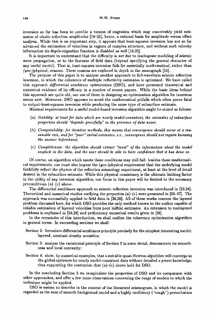
Computerm Math. Applic. Vol. 22, No. 4/5, pp. 147"-17"8, 1991 0097-4943191 $3.00 + 0.00 Printed in Great Britain. All rights Reserved Copyright(~1991 Pergamon Press plc

A D I F F E R E N T I A L S E M B L A N C E A L G O R I T H M F O R T H E I N V E R S E P R O B L E M OF R E F L E C T I O N S E I S M O L O G Y

WILLIAM W . SYMES* Department of Mathematical Sciences

PAce University, Houston, Texas 77"215-1892

A b s t r a c t - - This paper presents an an,dysis of stability and convergence for a special case of differential semblance optimization (DSO). This approach to model estimation for reflection seismology is a variant of the output least squares in~eraion of seismograms, enjoying analytical and numerical properties superior to those of more straightforward versions. We study a specialization of DSO appropriate to the inversion of convulutional-approxinmtion planewave seismograms over layered constant-density acoustic media. We prove that the differential semblance variational principle is locally convex in suitable model classes for a range of data noise. Moreover, the structure of the convexity estimates suggest a family of quasi-Newton algorithmA. We describe an implementation of one of these algorithms, and present some numerical results.

1. INTRODUCTION

Algorithms for solution of the seismic reflection inverse problem ("seismic waveform inversion") have been discussed extensively over the past several years; see, e.g., [1-7], for a small sample. All of the work just cited is based on the output least-squares principle, according to which a subsurface model is required to generate (synthetic) data which fit given data in the least mean-square error sense. This approach does not require picked travel times, unlike reflection tomography [8,9], and, in principle, could extract an optimal distribution of seismic velocities, as well as reflection amplitudes, unlike linearized inversion [10-13]. In addition, any desired level of detail concerning the physics of seismic wave propagation may be built into the output-least- squares principle, and it may also incorporate non-seismic constraints [14].

In practice, it has proven difficult to realize the apparent promise of least-squares inversion even when applied to synthetic data sets. Since the problems are computationally large, only iterative methods are feasible, and these require for their efficient convergence a measure of convexity often not possessed by the mean-square seismogram error (see, e.g., [1,15,16]).

The cause of this non-convexity is the extreme sensitivity of the synthetic seismogram to changes in the slowly-varying components of the velocity, as will be reviewed in Section 2. Thus, velocity trends emerge slowly or not at all as iteration proceeds, and the reflectivities are correspondingly degraded. For layered medium problems, Kolb and others have developed a number of continuation and reparameterization strategies which render the optimization more tractable [5,17]. Only limited tests of these devices (and no theoretical justification) have been reported, however, and it is difficult to understand how lateral heterogeneity might be accommo- dated by these techniques. Straightforward least-squares inversion of two-dimensional acoustic and elastic models has appeared to require a priori information of the gross model (velocity) features of very high quality and, when such information is provided, the results closely resemble those of carefully designed amplitude-preserving migration--unsurprisingly, as these are essentially equivalent [2,18,19]. In fact, the principal tangible result of the work on least-squares

*Research supported in part by the Office of Naval Research under con t r~ t N00014-89-J-1115, the Air Force Office of Scientific Research under contract AFOSP,89-0056 and by the National Science Foundation under grant DMS89-05878.

147

148 W.W. SYMES

inversion so far has been to provide a version of migration which may conceivably yield estimates of elastic reflection amplitudes [19-21], hence, a rational basis for amplitude versus offset analysis. While this is an important step, it appears that least-squares inversion has not so far advanced the estimation of velocities in regions of complex structure, and without such velocity information its depth-migration function is disabled as well [16,22].

It is important to understand that the difficulty is not due to inadequate modeling of seismic wave propagation, or to the features of field data (beyond specifying the general character of any useful model). That is, least-squares inversion fails for essentially mathematical, rather than (geo-)physical, reasons. These reasons are explored in depth in the monograph [16].

The purpose of this paper is to analyse another approach to full-waveform seismic reflection inversion, in which the coherence of multiple reflectivity estimates is optimized. We have called this approach differential semblance optimization (DSO), and have presented theoretical and numerical evidence of its efficacy in a number of recent papers. While the basic ideas behind this approach are quite old, our use of them in designing an optimization algorithm for inversion seems new. Moreover, DSO appears to avoid the mathematical pitfalls which often prove fatal to output-least-squares inversion while producing the same type of subsurface estimate.

Minimal requirements for a useful model-based inversion algorithm might be stated as follows:

(a) Stability: at least for data which are nearly model-consistent, the estimates of subsurface properties should "degrade gracefully" in the presence of data noise;

(b) Computability: for iterative methods, this means that convergence should occur at a reasonable rate, and for "poor" initial estimates, i.e., convergence should not require knowing the answer beforehand;

(c) Completeness: the algorithm should extract "most" of the information about the model implicit in the data, and the user should be able to have confidence that it has done so.

Of course, an algorithm which meets these conditions may still fail: besides these mathematical requirements, one must also impose the (geo-)physical requirement that the underlying model faithfully reflect the physics of the reflection seismology experiment, at least at the level of detail desired in the subsurface estimate. While this physical consistency is the ultimate limiting factor in the utility of any inversion algorithm, our focus in this paper will be limited to the necessary preconditions (a)-(c) above.

The differential semblance approach to seismic reflection inversion was introduced in [23,24]. Theoretical and numerical studies verifying the properties (a)-(c) were presented in [25-27]. The approach was successfully applied to field data in [28,29]. All of these works concern the layered problem discussed here, for which DSO provides the only method known to the author capable of reliable estimation of layered velocities from poor iniftial estimates. An extension to nonlayered problems is explained in [24,28] and preliminary numerical results given in [26].

In the remainder of this introduction, we shall outline the coherency optimization algorithm in general terms. In succeeding sections we shall:

Section 2: formulate differential semblance principle precisely for the simplest interesting model: layered, constant-density acoustics;

Section 3: analyse the variational principle of Section 2 in some detail, demonstrate its smoothness and local convexity;

Section 4: show, by numerical examples, that a suitable quasi-Newton algorithm will converge to the global optimum for nearly model-consistent data without detailed a priori knowledge; thus supporting the contention that (a)-(c) above hold for DSO.

In the concluding Section 5 we recapitulate the properties of DSO and its comparison with other approaches, and offer a few more observations concerning the range of models to which the technique might be applied.

DSO is easiest to describe in the context of the linearized seismogram, in which the model is regarded as the sum of smooth background model and a highly oscillatory ("rough") perturbation

Differential semblance algorithm 149

(reflectivity section). Note that the smooth background velocities are still regarded as part of the model, so it is still nonlinear. With some high-frequency approximations ("WKBJ Seismogram") the inversion of each common-source (or common-receiver or common offset) gather for a given background velocity may be accomplished semi-analytically (perhaps the best reference is [13]), by what amounts to an amplitude-preserving before-stack migration. If the background model is correct, presumably the images from the various inverted gathers will line up. If not, the discrepancy indicates that the background ("migration") velocity ought to be changed.

So far, this is hardly novel: a process called "iterative before-stack migration" is described in just this way in [30], for instance. The refinement leading to a feasible algorithm is the introduction of a well-behaved cost function, which we dub the differential semblance, which both measures the discrepancy between the various common gather inversions and indicates how the velocity fields should be changed to line them up (through its gradient). A natural choice is stack power or semblance [31], for example), but this leads directly back to the nonconvexity difficulties of output-least-squares: the two are very closely related [16, Appendix A]. Instead, we depend on the accurate inversion of amplitudes, and take the mean-square of the differences between successive inverted gathers. These differences should all vanish at the "correct" velocity estimate. Most important, as the background velocity is changed, this "differential semblance" (DS) changes smoothly, rather than abruptly, as is the case with stack power.

Two technical refinements are necessary to turn this idea into an algorithm. First, data noise which is uncorrelated from gather to gather will yield a very large contribution to the differences of the inverted gathers, completely distorting the DS and masking the correct choice of velocity. To avoid this oversensitivity to data noise, partly decouple the inverted gathers from the data: lump these reflectivities (one per gather) together with the background velocity field as the "model" to be determined, and redefine the cost to be the sum of:

(a) all of the mean-square data errors, i.e., differences between data seismogram and predicted seismogram based on the corresponding reflectivity section, and

(b) the mean-square sum of pairwise differences of reflectivity sections (DS).

Incoherent noise in the data gathers will be accounted for mostly in error-of-fit (i.e., (a)), as it should be, since it causes a much smaller increase in cost that way than when forced into the DS (i.e., (b)).

The second technical modification is required by the nature of the model-to-seismogram relation: as pointed out above, this relation is extremely sensitive to the background velocity component, when the model is defined in terms of depth (and offset). This oversensitivity is due to the time shift accompanying a change in background velocity, which causes the temporal location of a high-frequency reflection from a (depth-) fixed reflector to change. For a discussion of this "time-shift" disaster in the one-dimensional context see [32]. The remedy is clear: the reflectivity sections should be defined as time sections rather than as depth sections.

For the layered acoustic problem of this paper, it is rather trivial to accomplish this transformation. It is particularly convenient to work with plane wave sources, since the gather corresponding to a planewave source at definite slowness has only one independent trace. Thus a single reflectivity time trace at each slowness, together with the (single) background velocity depth profile, specifies the model. The reflectivity time traces are converted to depth traces through the (background) vertical travel-time-to-depth transformation appropriate to each slowness. The high-frequency approximation to the (p-tau) seismogram is simply the convolution of the time-trace refiectivities with the source wavelet, whereas the DS is essentially the derivative of the corresponding depth-trace reflectivities with respect to slowness.

For laterally heterogeneous models, the transformation from time to depth is less obvious. As explained in [25,29], the analogue of the travel-time-to-depth change of variables appropriate to plane waves in layered media is, in general, a before-stack Kirchhoff migration appropriate to the acquisition geometry being simulated, and the reflectivity gather is simply a time section. The differential semblance is a difference (or derivative) with respect to the shot location (for shot gathers) of the migrated refiectivity depth sections.

150 W . W . SYIdES

Two points remain to be emphasized. First, there is nothing to "cohere" unless reflectors are present, i.e., unless the reflectivity gathers are rich in high-frequency energy. As is the case with semblance, the differential semblance is a measurement of the portion of move-out in reflection phase not accounted for by the current velocity model. Therefore, the density of reflectors is a limiting factor in the recovery of accurate velocity models, as is the data aperture. These observations are quantified in Section 3.

Second, both DS and data misfit are summed in the cost functional for DSO. Thus both are minimized simultaneously. The major theoretical result of the paper (Section 3) is that, with appropriate weights on the two components, sufficiently dense reflectors and enough aperture, the cost functional is smooth and convex for near-consistent data. It also appears that due to the structure of these estimates, the selection of weights can be arranged to cause suitable quasi-Newton iterations to converge to the global optimum without accurate a priori knowledge. Numerical evidence for this assertion is given in Section 4; a corresponding theorem will be proved in another publication.

2. O U T P U T LEAST-SQUARES VS. D I F F E R E N T I A L S E M B L A N C E OPTIMIZATION

Denote the plane-wave ("p-r") seismogram corresponding to a velocity profile c(z) by S[c]. The arguments in this paper are based on the well-known convolutional approximation, which is reasonably accurate when c may be re-written as a sum

c ~, cs "l- Cr ,

where

cs(z) is a slowly varying background velocity model cr(z) is a rapidly varying "reflector sequence," having locally zero mean on the length scale of significant change in the background velocity.

Thus the (two-way) travel-time to depth z of a precritical plane-wave at (horizontal) slowness p is determined with a small error by the background velocity c, (z), according to

= 2 dz' c o . , , p2 = 2 Vs

where v is the vertical (plane-wave) velocity at slowness p:

1 _ p2 v, Cz,p) = c2(z) = c,(z)A(z,p),

A(z,p) = (1-c2,(z)p~) -112.

The convolutional approximation with (isotropic) source wavelet / ( t ) is then

S[cs,cr](t,p) = v(O,p)-i ( f . ~ - t ) ( t , p ) (1) 1 ~ t Or. ,

- v(O,p).u d t ' f ( t - t ' ) - ~ ( t , p ) ,

where the "reflectivity" r(t,p) is given by

r(t, p) = p), p) vs(¢(t,p),p)' (2)

by means of the inverse two-way travebtime function (, defined implicitly by

/ ~(t,p) 1 t - 2 - ,

,Io v


and the vertical velocity perturbation

vr -" Cr • A 3.

Note that reflectivity conventionally means Or/Ot; we shall confuse r and its t-derivative, calling both "reflectivity" as convenient.

Now S is clearly linear in Cr, but quite nonlinear in ca. In fact, a change in c, will typically result in a change in the "phase" ¢, and thus in a shift in the high-frequency components of S, which in turn derive from the high-frequency components in cr. Since such a phase-shift may have a drastic effect on components of the appropriate (high) frequency, and since cr must have a great deal of high-frequency content in order to model the dense distribution of reflectors in the typical sedimentary column, one expects S to be extremely sensitive to changes in the background velocity c,.

This oversensitivity to background errors shows quite clearly in the expression derived for the perturbation 6S in the seismogram, due to a perturbation 6c° in the background velocity (holding c~ fixed, and assuming 6c,(0) - 0):

6s(t,pl=v,(O,p)-~l, N - ~ 6 ~ , + ~ V, e (~(t, p), p),

where

~0 ~ ~ ( z , p ) := ~((~(z,v),p) = v,(z,p) dz',,,(z',p)c'i3(z')6e,(z ')

is the phase perturbation corresponding to or, referred to depth/slowness coordinates. Thus, the z-derivative of cr (or, of r) appears in the perturbations 6S associated with a

background velocity perturbation 6c8. On the other hand, a perturbation 6er in Cr simply results in

6s ~ S[c,, 6cr], as S is linear in cr--thus, no derivative of cr is involved.

Again, cr must be highly oscillatory to model the typical reflector distribution, so the derivative of cr is typically much bigger, in any reasonable sense, than is Cr itself. Thus, a perturbation of the background velocity cs has a much larger effect on S than does a perturbation of cr: in the language of linear algebra, the linear perturbation map ("Jacobian")

~Co, ~c~ ~ ~S

is ill-conditioned. Even worse, a straighforward extension of this reasoning shows that the difference between

the perturbed section Sic, + ~c°, c~ + ~e~]

and its linear prediction S[e,, c,] + 6S

can easily be on the order of S itself, even for quite small 6c. To summarize: under realistic assumptions on co and cr,

(i) the Jacobian 6S is ill-conditioned;

(ii) S is poorly approximated by its linearization.

Consequently, the output least-squares objective function

J[cs, er; Sdata] :-- / / dp dt [S[cs, er] - Sdata[ 2

is highly non-convex, with rapidly changing gradient, and the optimization problem

n~n g[~,, c,; Sd.,.] (3) CjtCr

152 W . W . SYME$

is extremely difficult to solve by means of any variant of Newton's method. For extensive discussion and illustration of these points, consult [16].

The crux of the difficulty is the interaction between the background cs and the reflectivity r through the definition (2). Accordingly, it is tempting to deconple co and r by treating r, rather than cr, as the "other" component of the model: thus define

0 r . , . SIc,, r](t,p) = v,(O,p) -1 S * -~( ,p).

Certainly, if r and cr are related by (2), then

s[c, , c,] = ~[~,, r].

In fact, apart from the surface normalization, the background velocity c0 enters the definition of S only implicitly, through the condition (2). If we are to use r as one of the independent variables, instead of or, we must develop a condition, phrased only in terms of c, and r, which guarantees that (2) holds. Fortunately, this is rather easy: from the useful identity

Vr ~ Cr

v, a - 4 ' (4)

it follows that, if (2) is satisfied, then

c73(~) ~r O) = v72( z, p) r(~(~, p), p). (5)

The notable quality of (5) is that the left-hand side is independent of p. Thus, differentiation with respect to p eliminates cr altogether:

o = ~p[vTffz,p) rC~O,p),p)]. (6)

It is easy to reverse this reasoning. Thus:

A section r(t,p) is the reflectivity corresponding to or(z) if and only if (6) is satisfied, in which case cr is given in terms of r(t,p) and c,(z) by (5).

In formulating the constraint given by (6), it is advantageous to return to (*,p) coordinates (the reason will become apparent below). Thus define the quantity W[c,,r] (the differential semblance) by

{ ° ) w[c.,rl(t,p) = N [v72(z'P) r(~(z'P)'P)] .=. , ,~) .

Then

if and only if

S i c , , ~.] = Sd:<:,

$[c, , r] = Sdat~, and w[c,,r] - 0,

with Cr and r related by (2) or (5). Since the problem is clearly overdetermined, it is commonplace to replace the exact fit of

predicted to measured seismograms by a best-fit condition. We shall follow the lead of most authors on this subject (e.g., [33]) and use the mean-square error measure, i.e., L 2 norms. Since derivatives are also involved in the definitions of important quantities, we also introduce some norms from the Sobolev scale, which measure the size of derivatives. Some notation for this is desirable: for a single z- or *-trace, e.g., f ( t ) , we write

,,,,, = ( i , ,< '>,O k

I I S l I I - lls<,l:, j=O

1/2


whereas for a (t,p) or (z,p) section, e.g., F(t,p), we write

IIIFIII ( / dt / dpp \112 = IF(t,p)l 2) ,

- lll lll +lll lll Integrations in all cases are over appropriate sets.

The weight p in the integral defining Ill III is a residue of polar coordinates, and is used to make the norm Ill III as close as possible to equivalent to the ordinary mean-square of an z-t section. See [16, Appendix nl; aiso [341.

In view of the equivalence noted above, it is natural to pose the constrained least-squares problem:

minimize IIl [c,, r] - s, t,,lll =, c, , r (7a)

subject to W[cs, r] =_ O.

This problem is closely related to the output least-squares problem (3). In fact, the relation is too close. The two problems have the same solution, and, in fact, are mathematically quite similar as well, so that (7a) is also poorly suited to computation. (For a detailed analysis of a simpler situation with similar features, see [25].) To obtain a problem which is not too "stiff," we "relax" (7a) by making the constraint W = 0 soft:

minimize J[c,, r, Sdata], (7b) cs,r

where

Y[c,, r, S,:t,,t,,] = r] - S t,,lll 2 + '2111w[ ,, r] III 2.

We shall call (7b) the differential semblance optimization problem. From the equivalence above, we see that if Sdat- is consistent, i.e., Sdata = SIc,, or], then the

problem (7b) has [es, r] amongst its solutions, for which r and er are related by (5). That is, for consistent data, (7b) has "the same solutions" as the output least-squares problem (3). We shall show, however, that (7b) is far better suited to numerical computation by Newton's method and its relatives. We shall also show that the solution of (7b) is stable, i.e., "degrades gracefully" in the presence of data error, for reasonable choices of the penalty parameter tr.

These conclusions are true, provided that Sdata is near (in the mean-square sense) to some "exact" or consistent data Sits, Cr], and provided that es, cr satisfy certain conditions. "Physical," or poetic, statements of these conditions are:

(i) c, should be "rough," i.e., contain significant variation (reflectors), on a length scale dictated both by the wavelet (.f) passband and by the smoothness (characteristic length) ore,;

(ii) The range of slownesses p available in the data ("aperture",) should be su~ciently large relative to both the degree of roughness mentioned in (i) and the amount of data error, so that the move-out of reflections clearly discriminates the velocities.

It is also necessary that the penalty parameter ~ be chosen appropriately. "Appropriate" means, so that the desired properties are obtained, i.e., so that Newton's method works (from a poor initial guess) and so that the solution obtained is relatively insensitive to data error. Note that in the limit cr --~ oo, (7b) becomes (?a), i.e, the constraint becomes hard. Previous remarks have indicated that (7a) is not susceptible to numerical solution through Newton's method or its relatives. Thus the possibility of choosing ~ "not too large" is crucial to the construction of algorithms which converge from a poor initial guess.

In the following section we will carefully quantify (i) and (ii) and justify these conclusions through an analysis of (7b). C&MWA 22:415-I (

154 W . W . SYM~.S

3. LOCAL CONVEXITY OF DSO

The local analysis of optimization problems amounts to the verification of several conditions concerning the first and second derivatives of the objective function. These conditions are imposed near a particular solution (i.e., local minimum) and guarantee that this solution is stable under data perturbations. The same conditions ensure rapid local convergence of Newton's method. We state the verbal description of these conditions here, together with the interpretation in terms of the quantities introduced in the last section:

(i) (Regularity) The objective function should be twice differentiable near the solution.

This is completely obvious for the seismogram error term IIl~[c,,r] -Sd~t~lll ~ as it is independent of cs and quadratic in r. For the DS, the regularity is suggested by the identity

a (vs(z,p)_ 2 r(v(z,p),p))lz=~(t,p) W[c,,r](t,p) = ap

{or o~t [,.... } (8) = -2pr( t ,p)+vT2(¢( t ,p) ,p) -~pp( t , p ) -p~( 'P)Jo v, .

Clearly, varying ca will have the effect of differentiating v , - -but c,, hence v,, is presumed sufficiently smooth that its derivative is not significantly larger than ca itself (we make this assumption precise below). On the other hand, no additional derivatives of r (the locus of high- frequency energy) result from varying c,. Thus W may be regarded as regular. Note that the perturbation of W would involve further derivatives of r if we had left off the final referral back to time/slowness coordinates.

(ii) (Second-order suITiciency) The objective Hessian is positive-definite.

Most of this section is devoted to verifying this last condition; it is the source of the requirements mentioned at the end of the last section.

The Hessian is the second-order coefficient 89-J in the power series expansion

c 2 ][c, + e ~c., r + , 6r, s~ t~ ] = ] [c , , r, Sd~t~] + , 6 ] + ~ 6 ~ ] + . . .

In view of the goal, enunciated at the end of the last section, to examine the perturbation of a consistent solution due to perturbing the data, we shall assume that

That is, that

][c,, r, Sd~t~] = 0.

Sic,, r] = Sdata and W[c,, r] = O. (9)

Let us state very carefully the meaning of the condition (ii) in terms of 62]: i.e., 82J is positive. Condition (ii) actually requires that 6~j be "positive relative to" ~c,,Sr: for some L > 0 ,

I]162J]11 >_ L (I]~c, II 2 + HI~rlH~). (10)

Indeed, as follows from the proof of the implicit function theorem, as L ~ 0 in (10), the size of the region of convexity of J goes to zero, and the possible ratio of solution error to data error goes to infinity. Thus, we need not only L > 0, but some positive control over L, to ensure stability (and computability) of the solution.

An easy calculation gives

69 2

Ill,. ' 111 •


Thus as a first requirement, we must have (for each p)

for some constant Kt > 0. Unless Kt is to be uselessly tiny, this means, in effect, that each trace ~r (p -- const.) (hence, eventually, ,) must have most of its energy in the passband of the source f , or else, that the out-of-band components must be constrained a priori. We adopt the first option: i.e., that we shall estimate only passband reflectivities. In quantitative terms, Kz should be at least some substantial fraction, say one-half, of the absolute moment of the wavelet (this choice is justified by the theory of convolution operators, and is essentially optimal):

K1 ~ . 5 f I]1. Inequality (11) only shows that 62f majorizes 111(86r)/(Ot)lll ~. Reference to (10) shows that

this is inadequate unsurprisingly, since we have not made full use of the hypotheses of (ii). To go further, we must introduce the linearized constraints (since otherwise 6e is unconstrained). As we have assumed ca, r, Sdata consistent, i.e., the system of equations (9), this simplifies considerably. The calculation is displayed in the Appendix: with cr given by (11), we obtain the identities

6W =$cW + brW, (12a)

Here the quantity O 6c is defined by

q 6 c : = [ 6 ( v o ¢ ) ] o ~ = A 3 6 c + c ' , ~ .

(We shall suppress the subscript "s" on ca whenever no confusion is possible.) Also, we have used the useful notation

g o ~ ( z , p ) = g C ~ C z , v ) , p )

for (any) function g(t,p) and, similarly, for the symbol o ~. The further analysis of this condition in general is a little involved. We consider in detail only

the special case e (hence v) constant for z >_ z0 (13) 8c (hence 6v) _= 0 for z _< z0.

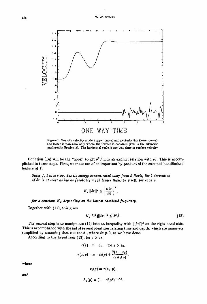
A few remarks about the general case appear near the end of this section. See Figure 1. Under this restriction, 5cW simplifies considerably: Q 6c = A a 6c, and

Now

0~A u = 2pcUA 4.

Thus what remains of (12a) is an exact derivative in p, so we integrate in p from Pl to p~ to obtain

o•pP2 = v-2(6,o~)1~: + ep(6oWo ~) l f"

- - ~-'A-'(6,o,-)l; ~ + dp(~oWo,-). 1

(14)

1 5 6 W . W . SYMES

i i ! i i i i i ! 2 .4

2 .2

2.11

1.8

I . b

E-~ I - - t I 4 r j ( ~ 1.2

> .El

. 4

2

- 2

0 ' I I I t I t I I

1 ~ 3 d

! I ! t ! t

5 5 7 8

O N E WAY T I M E

F i g u r e 1. S m o o t h v e l o c i t y m o d e l ( u p p e r c u r v e ) a n d p e r t u r b a t i o n ( l o w e r c u r v e ) : t h e l a t t e r i s n o n - z e r o o n l y w h e r e t h e f o r m e r is c o n s t a n t ( t h i s is t h e s i t u a t i o n a n a l y s e d i n S e c t i o n 3) . T h e h o r i z o n t a l s c a l e is o n e - w a y t i m e a t s u r f a c e ve loc i ty .

Equation (14) will be the "hook" to get 62j into an explicit relation with gc. This is accomplished in three steps. First, we make use of an important by-product of the assumed bandlimited feature of f :

Since f , hence r, 6r, has its energy concentrated away from 0 Hertz, the t-derivative of 6r is at least as big as (probably much larger than) 6r itself: for each p,

I o. K2116rll 2_< 0t '

for a constant K9 depending on the lowest passband frequency.

Together with (11), this gives

K2 K~ 1116rill 2 _< a2j . (15)

The second step is to manipulate (14) into an inequality with Ill,rill 2 on the right-hand side. This is accomplished with the aid of several identities relating time and depth, which are massively simplified by assuming that e --- coast., where 6c # 0, as we have done.

According to the hypothesis (13), for z > zo,

c(z) = cl, f o r z > z o ,

2(z - z0) ~ (z ,p) = ~0(p) +

C l A l ( p ) '

where

and

~0(p) = ~(z0,p) ,

A1Cp) = (1 - c~ p ~ ) - 1 / 2

! 6 C~

~ ' ~ 1.4

E ~ I 1.2

I.---4

0 1.8

> 8

6 <

<

0 i l i l l l 8 1 2 3

' I ' I ' I ' I ' I I " I " I ' I l I '

I gll l ' I ' I

t~ -X- qo

C ) 7w

>

4 .5 b 7 8 9

11 "1 "1 NOI~MALIZI~D SLOWNESS

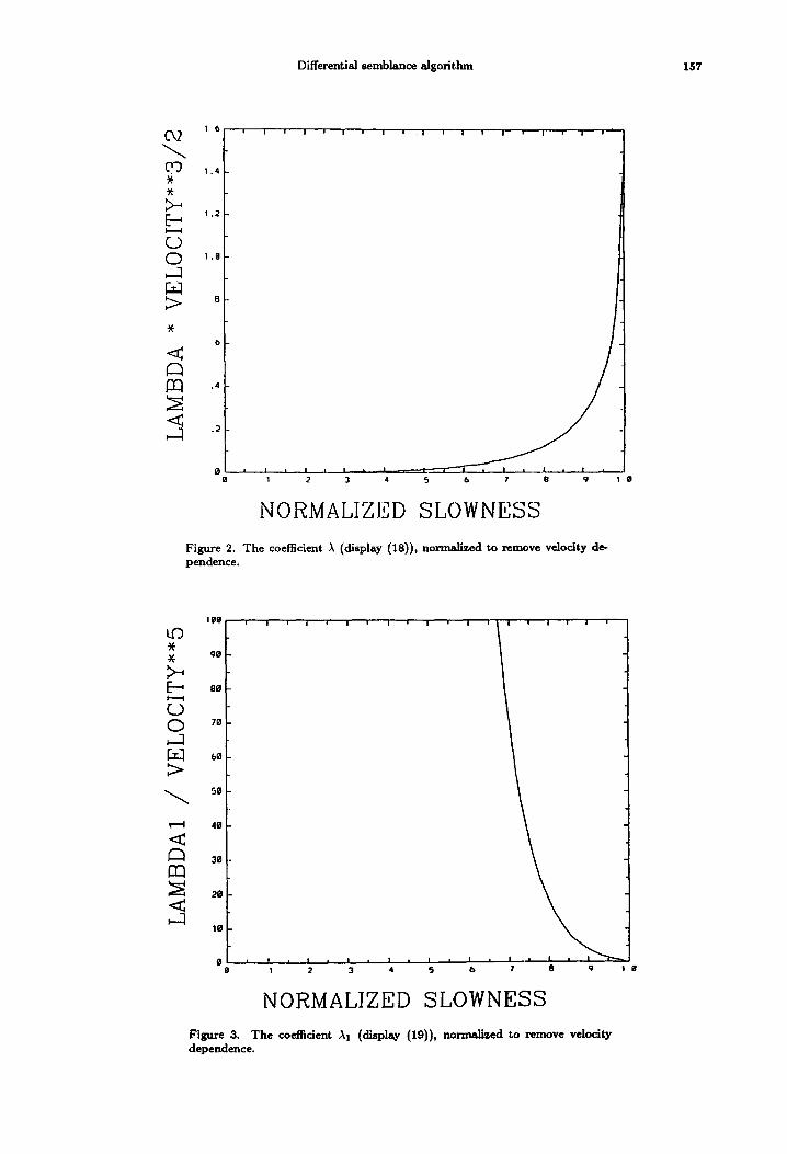
Figure 2. The coefficient ), (display (18)), normalized to remove velocity dependence.

~ se

4e

< 3e

I 2 3 4 5 b 7

. | w I I | I l z I ' l ! I

8 9


NORMALIZED SLOWNESS

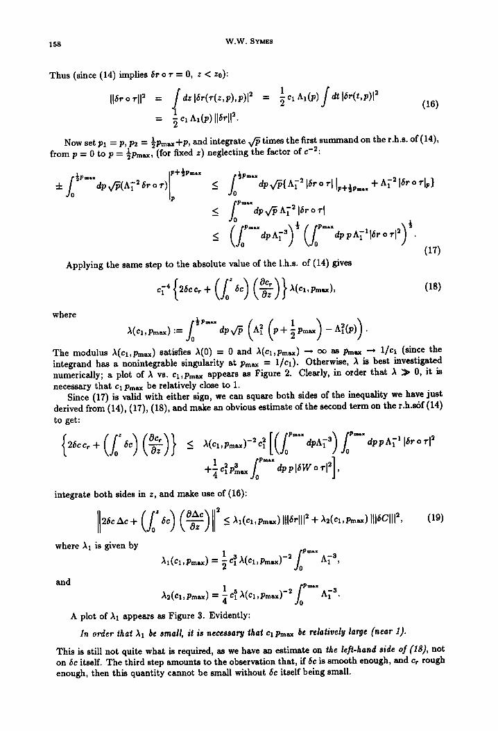
Figure 3. The coef~cient Az (display (19)), normalized to remove velocity dependence.

158 W.W. SYMES

Thus (since (14) implies 6r o r = 0, z < z0):

/ IClAI(p)f dt'6r(t'p)'2 116r°rll2 = dz l6r(r(z 'P) 'p)12 = ~ (16)

= ~ Cl At(p)ll~rll 2.

Now set Pl = P, P2 = ~Pmax +P, and integrate V~ times the first summand on the r.h.s, of (14), from p : 0 to p -- lpmax, (for fixed z) neglecting the factor of c-2:

½p.. lP+½ P-" / ½ p - - :h / dpv~(A'~26ror)] <_ dPv~lA-{216r°rll,+½,..+A;216r°rl,} JO P JO

< f o P ' " d p v ~ At216~ o rl

<_ (ff'"dpA'~a) ½ (fo'"fdppA'~',6rorl 2) ½. (17)

Applying the same step to the absolute value of the l.h.s, of (14) gives

~(Cl, Pmax), \ a z / . (18)

to get:

{26CCr+(foZ6C) (Scr~Sz)j < ,,~(c1,Pmax)-2c21[(j~oPm'=dpA13)j~oPmlXdppA1116r°T12 Cl Pmax +_ 2 s dp p ]6W o r[ 2

integrate both sides in z. and make use of (16):

ll2~cAc+ (~z~c) (~gc)ll2 ~1(cl,Pmax)]r~r[]12 +,~2(Cl,Pmax)[]]~CHl2 , (19)

where ~z is given by

1 3 fo p~x ~dCl,Pm.=) = ~ Cl A(Cl,Pmix) -2 A~ "s,

and I 5 ~P="

~2(CI, Pmax) = ~ Cl ~(Cl, Pmax) -2 A13.

A plot of ~1 appears as Figure 3. Evidently:

In order that Ax be small, it is necessary that cx pmax be relatively large (near 1).

This is still not quite what is required, as we have an estimate on the left-hand side of (18), not on 6c itself. The third step amounts to the observation that, if 6c is smooth enough, and cr rough enough, then this quantity cannot be small without 6c itself being small.

where

A(Cl,pm,x) dpV/'P V+ ~ " The modulus A(Cl,Pmax) satisfies A(0) = 0 and ~(Cl,pmax) ~ OO aS Pmax "-* 1/cl (since the integrand has a nonintegrable singularity at pmax = 1/Cl). Otherwise, ~ is best investigated numerically; a plot of ~ vs. cl ,pm~ appears as Figure 2. Clearly, in order that A ~ 0, it is necessary that cl pmx be relatively close to 1.

Since (17) is valid with either sign, we can square both sides of the inequality we have just derived from (14), (17), (18), and make an obvious estimate of the second term on the r.h.sSf (14)


This observation is the most physically-meaningful, and the most difficult to quantify, of the points presented in this paper. As illustrated thoroughly in [16], the local behaviour of the seismogram function near a. rough model is quite different from that near a smooth model, and it is this property that is being used implicitly at this point.

A rigorous semiquantitative treatment of roughness is found in [27], and the present problem can be treated along the same lines. Such rigorous argument is neither particularly enlightening, however, nor very precise. For the present, a numerical illustration of this property will suffice. The smoothness of the velocity model c and its perturbation are guaranteed, for example, by insisting that

c(~) = coexp x~¢~(~) ,

N

6c(~) = ~ 6~s cs(~). ~(~), j= l

where {¢j } is a finite, smooth set of basis functions. In the tests reported in Section 4, cubic b-spline integrals are selected for the {¢j }: these have associated with them a definite length scale ("width"); see Figure 4. Then in vector notation,

where

ll6ce, ll 2 = 6,T R o ~

is the N x N symmetric positive-semidefinite "roughness matrix" associated with Cr and the basis {¢~}.

Similarly, 116C]} 2 "- 6 z T M 6z

and

where

I oc,, ' o~ II = 8~TR( ' ) ,5~,

and M is the symmetric positive-definite "mass matrix"

Mi.~ = / dz ¢i(z) ¢s(z) C2(Z).

It follows that p(o~ 116cll 2 > 116cc~11 ~, (2Oa)

where p(m ° ) >_ 0 is the largest eigenvalue of the N-dimensional generalized eigenvalue problem

R (°) y = p M y. (20b)

Likewise,

- az II '

where P~n is the least eigenvalue of the generalized eigenvalue problem

(2oc)

R (z) y = p M y. (20d)

1 6 0 W . W . SYMES

I--'-4

<~

7O

b5

• 68

• SS

. SO

45

48

35

3e

• 25

.20

.15

10

05

0 O

l i

i #

s~ s j 1

: , i i i t , ,,

i

' i i i i : ,

t t i i f i w t

: , I i

f I

I

t t

.1 2 3 4 5 5 7

O N E W A Y T I M E

F i g u r e 4 a . C u b i c b - s p l i n e s : 5 t h ( s o l i d ) a n d 7 t h ( c l a s h e d ) o f 1 2 n o d e s i n t h e

i n t e r v a l

f-~

I ---4

07g

065

.ebO

.055

.eSO

845

048

e35

• 036

.e25

.e~'o

. o l 5

005

0

I I I s I i I ' I i

3 .4 ,, '2 .'~ , , . ;

O N E W A Y T I M E

F i g u r e 4 b . I n d e f i n i t e i n t e g r a l s o f s p l i n e s i n F i g u r e 4 a .


Finally,

Oz ' (20e)

where/4mi n is the least eigenvalue of the generalized eigenvalue problem

R y := (2R (°) + R (')) y = p M y . (20f)

Combining (19), (20a), (20c) and (20d) we get

mi. Ilacll 2 < A (c ,pm )1116 111 + . 2(Cl,Pmsx)1116Will 2 (21a)

and

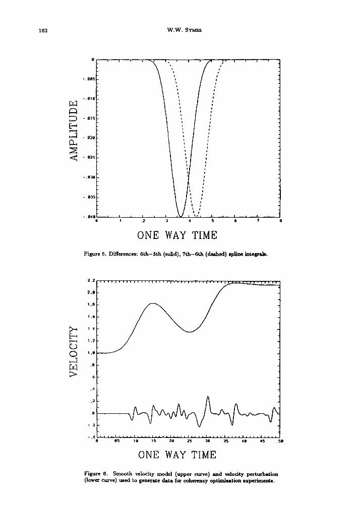
Obviously, inequality (21b) has force only ifP(ml~n >> p(m °), that is, Ocr/Oz is much bigger than cr, whence cr must be rough. In fact, Cr must be uniformly rough on the length scale of significant variation in c. To see this, note that the worst possible situation is when R (°) and R (t) have a common null vector, since then the left-hand side of (19) constrains the corresponding component not at all. This can indeed occur. Note that the integrated spline basis {¢1 } is so constructed that Cj - ¢j+I vanishes outside an inteval lj, encompassing five spline nodes: see Figure 5. Suppose that for some j, Cr = 0 in the interval lj: that is, there are no reflectors in 1 i. Set 6x I = I, ~Zjq-1 - - -1 , 5zi -- 0 for i ¢ j , j + 1. Then R c/) 6z = 0, j = 0, 1, so p = 0 with eigenvector 6z for both matrices. Thus:

In order that • (z) A. (o) /'~min > "Xl"max ~> O, significant reflectors must be present .in every depth interval of the characteristic length scale of the smooth model class.

In fact, it turns out that this condition is also necessary in order that the "combined" eigenvalue flrnin be reasonably large, as we shall see below.

Note also the connection with the wavelet passband. In order for the convolutional model to be accurate, e must have almost all of its energy concentrated below the passband (or rather its spatial analogue): that is, e must be smooth on the spatial wavelength scale. Suppose that c is chosen to attain, roughly, the maximum degrees of freedom permitted by this constraint. Thus, the length scale associated with the background model is roughly the largest spatial wavelength in the data, and we can re-phrase the above conclusion as:

In order that (19) above constrains 6e, significant reflectors must be present in every depth interval longer than the longest spatial wavelength in the data.

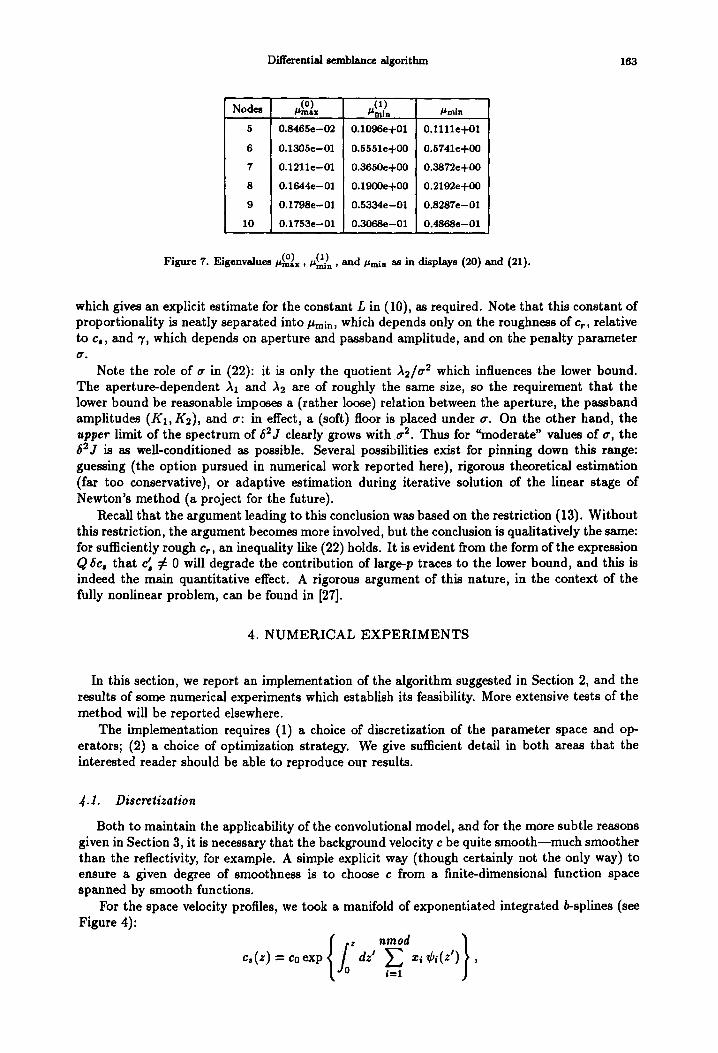
This necessary condition is actually also sufficient, when made appropriately precise ([27]; see also [16]). We illustrate the sufficiency by introducing the reflector sequence cr figuring in the experiments of Section 4. See Figure 6. We have computed the extreme eigenvalues of the problems, (20b), (20d), (20e). For an N-dimensional integrated spline space, the characteristic

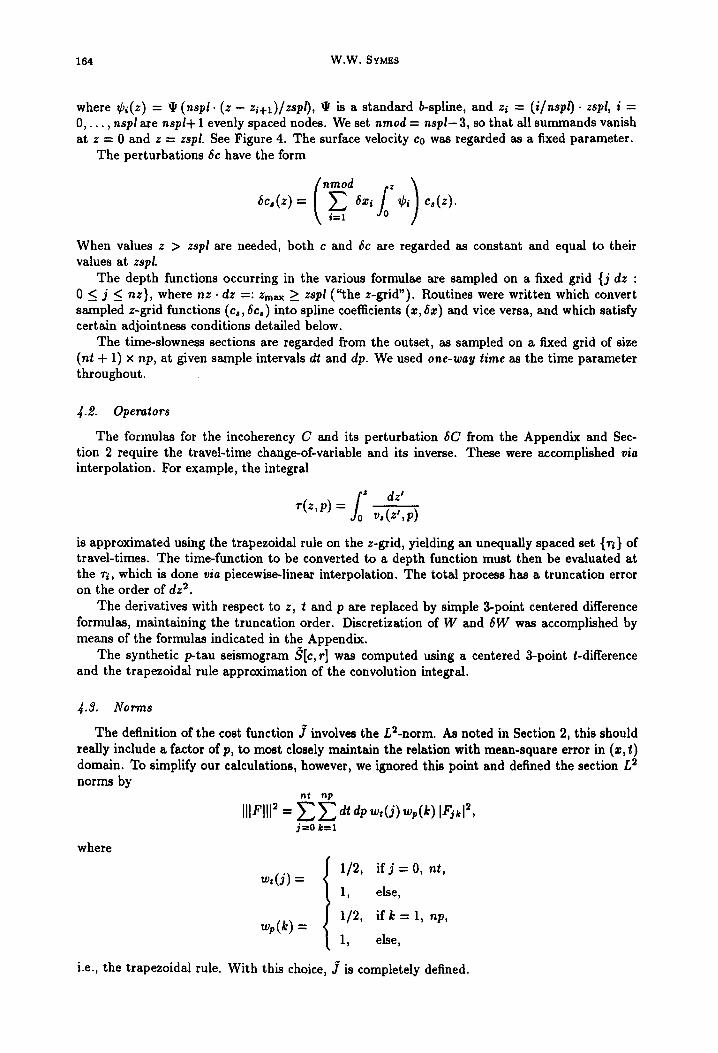
length scale (i.e., the length of Ij) is proportional to 1IN. In Figure 7, we tabulate p(m ° ) ,

P~n and Pmin against N, along with the characteristic length scale; for the background velocity profile we have taken the profile in Figure 6 also. We have not restricted the non-zeros of 6e to the c = const, segment, so this is a more severe test than warranted by the present discussion. Evidently, the criterion above is indeed sufficient to guarantee p(mX]n -4p(m°)ax > O in this case and appears necessary to have #Mrnin ~>~ 0.

We now combine the conclusions of three steps: (13), (19), (20e), to get

A1 A2 Umi,7 116c112 - </ i2J ' 7 = Ks K----~ + a 2'

and, using (15) again,

1 Pmin (116cll 2 + 1116rill _ 62j , mm 2"r ) (22)

162 W . W . SYMES

- . B 0 5

- . ~ 1 0

- 8 1 5

- g 2 0

- B 2 5

- . 0 3 0

- . 8 3 5

- 0 4 0

ONE WAY TIME

i I I

P - - t

<~

i #

/

i s

I I s l q !

m

f

i/ w

I I I i I i I " " t ! 2 4 S

i

Figure 5. Differences: 6th-Sth (solid), ? th-6 th (dashed) spUne integrals.

I l i a I I I SJ I l l I l l I l l l I I I . . . . ~ J . . J _ . ~ m l l e l l m I . I

0 0

;>

2 2

2 . e

1 . 8

1 . b

1 4

1 . 2

I . @

. 8

6

I

.4

.2! e !

- 2

- . 4 0 OS 1 O 1S 2 0 2 5 30 3 5 4 g 45 . SiP

ONE WAY TIME

Figure 6. Smooth velocity model (upper curve) and velocity perturbation (lower curve) used to generate data for coherency optimization experiments.


Nodes

5 0.8465e-02

6 0.1305e-01

7 0.1211e--Ol

8 0.1644e--01

9 0.1798e-01

10 0.1753e-01

0.1096e+01

0.5551e+00

0.3650e+00

O.1900e-t-O0

0.5334e-01

0.3068e-01

0.1111e+Ol

0.5741e+00

0.3872e+00

0.2192e+00

0.8287e-01

0.4868e-01

Figure 7. Eigenvalues ~(m°)x, .(ml)n, and ~min as in displays (20) and (21).

which gives an explicit estimate for the constant L in (10), as required. Note that this constant of proportionality is neatly separated into ~min, which depends only on the roughness of cr, relative to c,, and 7, which depends on aperture and passband amplitude, and on the penalty parameter ft.

Note the role of ~ in (22): it is only the quotient A2/a 2 which influences the lower bound. The aperture-dependent Ax and As are of roughly the same size, so the requirement that the lower bound be reasonable imposes a (rather loose) relation between the aperture, the passband amplitudes (K1, Ks), and a: in effect, a (soft) floor is placed under or. On the other hand, the upper limit of the spectrum of 6sJ clearly grows with a s. Thus for "moderate" values of ~, the 6~J is as well-conditioned as possible. Several possibilities exist for pinning down this range: guessing (the option pursued in numerical work reported here), rigorous theoretical estimation (far too conservative), or adaptive estimation during iterative solution of the linear stage of Newton's method (a project for the future).

Recall that the argument leading to this conclusion was based on the restriction (13). Without this restriction, the argument becomes more involved, but the conclusion is qualitatively the same: for sufficiently rough cr, an inequality like (22) holds. It is evident from the form of the expression Q6c, that d, ¢ 0 will degrade the contribution of large-p traces to the lower bound, and this is indeed the main quantitative effect. A rigorous argument of this nature, in the context of the fully nonlinear problem, can be found in [27].

4. NUMERICAL EXPERIMENTS

In this section, we report an implementation of the algorithm suggested in Section 2, and the results of some numerical experiments which establish its feasibility. More extensive tests of the method will be reported elsewhere.

The implementation requires (1) a choice of discretization of the parameter space and operators; (2) a choice of optimization strategy. We give sufficient detail in both areas that the interested reader should be able to reproduce our results.

J.1. Discretization

Both to maintain the applicability of the convolutional model, and for the more subtle reasons given in Section 3, it is necessary that the background velocity c be quite smooth--much smoother than the reflectivity, for example. A simple explicit way (though certainly not the only way) to ensure a given degree of smoothness is to choose c from a finite-dimensional function space spanned by smooth functions.

For the space velocity profiles, we took a manifold of exponentiated integrated b-splines (see Figure 4):

{/0z } c ° ( z ) = co e x p dz' ¢ i ( z ' ) ,

164 W.W. SYM~S

where ¢i(z) = ~ (nspl. (z - zi+l)/zsp O, @ is a standard b-spline, and zi = (i /nspl). zspl, i = 0 , . . . , nspl are nspl+ 1 evenly spaced nodes. We set nmod = nspl -3 , so that all summands vanish at z = 0 and z = zspl. See Figure 4. The surface velocity e0 was regarded as a fixed parameter.

The perturbations/Se have the form

/ nmod z )

\ i= l

When values z > zspl are needed, both c and 6c are regarded as constant and equal to their values at zspl.

The depth functions occurring in the various formulae are sampled on a fixed grid {j dz : 0 < j <_ nz}, where nz • dz =: zmax > zspl ('%he z-grid"). Routines were written which convert sampled z-grid functions (c,, 6c,) into spline coefficients (z, 6z) and vice versa, and which satisfy certain adjointness conditions detailed below.

The time-slowness sections are regarded from the outset, as sampled on a fixed grid of size (at + 1) x np, at given sample intervals dt and dp. We used one-way time as the time parameter throughout.

4.2. Operators

The formulas for the ineoherency C and its perturbation 6C from the Appendix and Sec- tion 2 require the travel-time change-of-variable and its inverse. These were accomplished via interpolation. For example, the integral

fo z dz~ = v.(z,,p)

is approximated using the trapezoidal rule on the z-grid, yielding an unequally spaced set {ri} of travel-times. The time-function to be converted to a depth function must then be evaluated at the ri, which is done via piecewise-linear interpolation. The total process has a truncation error on the order of dz ~.

The derivatives with respect to z, t and p are replaced by simple 3-point centered difference formulas, maintaining the truncation order. Discretization of W and 6W was accomplished by means of the formulas indicated in the Appendix.

The synthetic p-tau seismogram SIc, r] was computed using a centered 3-point t-difference and the trapezoidal rule approximation of the convolution integral.

4.8. Norms

The definition of the cost function J involves the L2-norm. As noted in Section 2, this should really include a factor of p, to most closely maintain the relation with mean-square error in (z, t) domain. To simplify our calculations, however, we ignored this point and defined the section L 2 norms by

n~ np

IIIFlll 2 = dp w,(j) w,(k)IF kl 2, j--0 k--1

where

=

wp( ) =

1/2, if j = 0 , nt,

1, else,

1/2, if k = l , np,

1, else,

i.e., the trapezoidal rule. With this choice, j is completely defined.

Differential semblance algori thm 165

The importance of choice of norms in the model space It,, r] cannot be overemphasized. Even though the definition of ] is independent of this choice, it is the main factor affecting the e1~iciency of the optimization. This is principally because of the role of the model norm in the definition of the gradient. We examine this point for the summand ~r 2 IIIW[c, 1"] III z of ] , since it involves both c and r. By definition, the gradient of this term is the (unique) model vector [~, ÷] for which for any [8c, dfr],

lim I (~2 I I I W [ ~ , , + ~ , , ~ + ea~]lll2 - ~2111w[~,, r]ll12 ) -- ((~,, ÷),(so,, 6r))M, (23) ~--*0

where ( , ) M is the scalar product in model space corresponding to the norm:

II [6c,, 6~] ll~ = ([6~o, a~], [6~,, a~])~.

(We assume that the model space is a Hilbert space, since all efficient smooth optimization methods are predicated on this assumption.)

A principal requirement ((i) in Section 3) is that the function It,, r] ~ III W[e, r] III ~ is regular, i.e., differentiable. Examining (A.2), we see that derivatives of 6r are involved in dfW. Since r, 6r are to be allowed to be arbitrary (grid-representable) functions, ~W can ony be continuously dependent on 8r, as is required by regularity, if the model norm includes explicit control over derivatives of Er. The obvious choice for the section part of the model norm is

n t np

116rl[~ -- ~ ~ dtdpwt(j)wp(k) { 16rjkl z + ID, 6rSkl 2 + IDp 6 r~klz}, j----0 k = l

where Dt and Dp are 2-point one-sided difference approximations for ~/~t and dg/~gp. The subscript "1" stands for "first derivatives"; this is the discrete version of the first in the Sobolev scale of norms, a basic tool in modern analysis of partial differential equations.

For the velocity profile part, i.e., 6e, we can make use of the fact that c is required to belong to a space of smooth splines.

We enforce the membership of c in the spline manifold by parameterizing the model in terms of the spline coefficients zi themselves, rather than the z-grid values of c. Also, we tacitly use logc, and its perturbation, 6c, /c , , as fundamental quantities, rather than c, and 6c,; this nondimensionalizes that part of the model (note that r is already non-dimensional, by definition). Thus, we need to express the norm of 5c,/c, in terms of the dfxi; this is easily accomplished via the mass matrix

Mi~ = ] dz ¢i ¢i.

This is computed via the trapezoidal rule, of course. Then

L 6Cs 12 -- 6xT M dfx. {laz e, L~

Note that we are measuring (O/•z)(6c,/c,) rather than (6c, /c,) itself. Since 6c,(0) -- 0, a bound on the former implies a bound on the latter, but the choice we have made here weights the more oscillatory velocity perturbations more highly, and, thus, tends to rotate the gradient in the direction of smoother 6c,'s, with favorable computational consequences.

Now regarding the model as the pair [z, r] (rather than [e, r]), the model norm is taken to be

II [6x, dfr] 112M -- Pc 5z T M 6x + Pr 116rll~.

Adjustment of the weights Pc, Pr allows the gradient to be rotated in the z- or r-directions; this scaling-preconditioning turns out to be important in achieving rapid convergence.

166 W . W . SYMES

4.4. Gradients, Hessians

First examine the incoherency component of ] , as before. To write the result in a revealing way, recall that 6W is linear in [6z, 6r], and write 6W. [6z, 6r] for the value. Then the limit on the 1.h.s. of (23) can be carried out to give

2~ 2 {6W . [6x, 6r1, W[x, rl) L~ -" ([6x, 6rl, 2a 2 6W" . W[z, r]) M , (24)

where the adjoint operator 6W* is defined by the condition

(6W[6z, 6r], F) L 2 = {[6z, 6r], 6W* . F) M , (25)

which is to hold for arbitrary model perturbations [6x, 6r] and (t, p)-sections F. Comparison of (23) and (24) reveals that

grad( IIIWIII2) = [i' ÷] (26a) = 2a 2 6W* • W.

Likewise, the Gauss-Newton approximate Hessian operator [35, Section 10.2] is given by

Hess(a 2 IIIWHI2) • [6x, 6r] = 2a 2 6W*. 6 W . [~z, 6r]. (26b)

Similar formulas hold for the term IHS- Sdata]ll 2. The calculations (26) are the principal parts of the quasi-Newton methods to be introduced

below. Thus efficient and accurate calculation of the adjoints 8W*, 6S* are essential to a suc- cessful optimization.

4.5. Adjoints

The definition (25) of 6W* must be taken absolutely seriously. That is, even though 6W is given (in principle) by an enormous matrix, 6W* is not simply the operator defined by the matrix transpose of 6W. In fact, 6W* is related to the matrix transpose and this relation provides a convenient avenue for computing 6W*.

The scalar products involved in (25) may be written symbolically in the form

( X , Y ) a = X T GY,

where X and Y are parameter vectors and G is the Gram matrix of ( , )a. Thus, G is a positive-definite symmetric matrix of size equal to the dimension of the parameter space.

In the cost of the functional ] , two essentially different inner products are involved, on two different parameter spaces (models [6x, 6r], sections F), as well as a linear transformation (~W) mapping one parameter space into the other. Accordingly, consider two inner products of the form given above, with Gram matrices Gv, v = 1, 2, and a linear transformation A, given by a matrix of appropriate dimensions, mapping one parameter space into the other. The adjoint of A is defined by:

(A X1, X2)a , = (X1, A* X2)a2

for arbitrary Xv in the v th parameter space, v -- 1,2. Written in matrix form,

(A X l ) T G1 X2 = X T G2 A ° X2,

from which it is clear that, as matrices,

A* = G~IATG1. (27)

To see what (27) implies for (25), write 6C in components:

6 w = [6 w,


dll

3S

E-,

25

2e

(. . , z I----4

I l l

05

O - OS O i lS 10 t 5 2 0 2 5 3 0 35 4 0

SLOWNESS

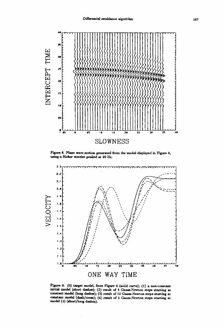
Figure 8. Plane wave section generated from the model displayed in Figure 6, tudng a l~cker wavelet peaked at 20 Hz.

O

2.3

2 . 2

I g

1.8

t . 7

.6

5

.4

,3

.3

. I

g

~ ~P so" / ',, r , , A • u

/ ,3 ,

v / \~ ,~ , ,

/ /11/ ,

If// , a

¢o

¢

o u o

,I

#

OS 10 15 2 0 2 5 30 3 5 4 J 4 5 5 0

ONE WAY TIME

Figure 9. (0) target model, from Figure 6 (solid curve); (1) a non-constant hfitial model (dlort da~es); (2) result of 5 Gauss-Newton steps starting at constant mode] (long daJuttes); (3) result of 10 Gauss-Newton steps starting at constant model (da~/crmm); (4) result of 5 Gauss-Newton steps starting at model (1) (short/Ioag dashes).

168 W.W. SYMES

This is the correct matrix representation if the model perturbation is written as a column vector:

6W. = 6=W.6z + ~,W.6r . 6r

Thus,

where

and

(6=W. 6z, F) L2 = 6zT M (6=W* • F) (28a)

(6rW. 6r, F)t.2 = (6r, 6rW*. F)t . (28b)

Identify a section F with a vector in any convenient fashion, e.g., by listing the traces (columns) sequentially. Then the L2-inner product, discretized by the trapezoidal rule, is realized by the scaling matrix S (which scales the edge entries by 1/2, the corner entries by 1/4, and everything else by 1):

for any sections F1, F2. Thus (27) applied to (28a) gives

(F1,F2)~ = fr~ S F2

6=W ° = M -1 6=W T S. (29a)

For (28b), it is necessary to write the "Sobolev" inner product ( , ) 1 in the canonical form given above; its Gram matrix turns out to be exactly the matrix of the discrete Neumasn problem for the usual five-point discretization of the Laplace operator, which we shall denote by N. Thus

6r W* = N - 1 ~ W T S. (29b)

In principle, this completes the calculation of the adjoints, hence of the gradient and Hessian. In practice, inspection of (26a,b) shows that we need only routines which apply 6W* to a vector [6z, 6r], not the entire matrix of 6W*. This extremely important observation saves much computational effort and storage. In fact, application of the trapezoidal scaling operation represented by S is trivial, and the transpose operations 6=W T, ~rW T are relatively easy to work out, as the same sort of recurrence rules that form the '~forward" calculations of 8=W, 8rW. Thus we represent (29a,b) in the alternate forms: for an arbitrary section F,

6 c W * . F = ~, (30a) M z = 6 = W T S F ,

6 r W * ' F = ÷, (30b) Ni" = 6 r W T S F .

We have just described how to compute the right-hand sides of the second equations in each of these pairs. To solve the linear system with the spline mass matrix M, we used a standard linear equation solver (LINPACK: SPOFA, SPOSL), as the spline space is small-dimensional--i.e., the background model has few degrees of freedom, <_ 20 in all of our experiments. To solve the discrete Neumann problem, which is quite large (nt = 300, n p = 40 in some experiments), we took advantage of explicit knowledge of the discrete Neumann eigenfunctions (tensor-product cosines) to design an FFT-based discrete Neumann solver, which solves the second member of (30b) very efficiently.

This step would have been more difficult if the factor p had been included in the integral defining ( , ) z , as it should be. Then N would include a p-difference approximation to the Bessel operator of order zero, with Neumann condition at p - Pmax (a residue of the cylindrical geometry implicit in the proper definition of the Radon transform). Thus, fast Bessel transform software would be required.


4.6. Interface with the Optimizer

Since the optimizer described below accepts standardized n-vector arguments, it was necessary to "bundle" the computations just described into procedures with standard calling sequences. We used a pack/unpack routine, which collapses the spline/section pair [6x, 6r] into a vector of length nspl + (nt + 1) * np, and vice versa.

4.7. Choice of Optimizer

The tests reported below were made using a so-called truncated Newton code. This code is based on the model trust region principle [35, Section 6.4] and on the extensions to it introduced by Steihang in his Yale thesis [36]. Essentially, the Gauss-Newton linear step

Hess J . [6z, 6r] = -grad ff

is solved by a conjugate residual iteration [37, Chapter 10], which is terminated when the step estimate exits a ball about the current solution estimate, the radius of which is determined by a simple and robust updating strategy. This expedient avoids expensive conjugate residual steps taken outside the region in which the linearized model can be "trusted," hence the name. A more lengthy description of the code can be found in [16, Chapter 9], where the same codes were used in solving the nonlinear output least-squares problem, using finite difference synthetic seismograms instead of the convolutional model.

An important amendment of the trust region idea is natural in this problem. All models in the iteration are supposed to have a fixed rectangle [0, tmax] × [0, Pmax] as a precritical set. This may cease to be true during an update step, if the velocity is increased by too much at some depth. The computation of the gradient simply flags this occurence, and the algorithm attempts a smaller step in the same direction. Thus the trust region, for problems like the present one, may involve in a natural way constraints on the validity of the model itself.

4.8. Numerical Experiments

We performed a number of numerical experiments using the velocity profile e (upper curve) and perturbation cr (lower curve) exhibited in Figure 6 to generate the p-tan convolutional model data of Figure 8, by convolving with a Ricker wavelet with center frequency 20 Hz. A target background velocity with a lower velocity zone was chosen because the structure of such a zone is impossible to determine from refraction arrival times, and intrinsically more difficult for least-squares methods--see [16]. The velocity, hence the slowness, were normalized against the surface velocity, by changing the measure of depth to normal-incidence time, for a constant background velocity equal to the surface velocity. This step also normalizes the slowness to the range 0 < p < 1. A happy side-effect of this normalization was to reduce substantially the numerical imprecision resulting from mis-scaling inherent in the use of physical units.

The algorithm explained in the preceding subsections was used to extract estimates of es and r from the data of Figure 8. Parameters common to all experiments were

or= 1, /~e = 10 -4 , Pr = 1.

We found the small value of Pe necessary to rotate the gradient of J toward the "es-"direction. In all cases, we observed the same pattern. We began with the simple estimate Cinitial " "

const. (-- 1), rinitial = 0. The first Newton step did not change the estimate of e0, since the incoherence of r = 0 vanishes for any velocity model. Otherwise put, since there are initially no reflectors, there is initially no move-out information in the reflectivity with which to update the velocity model. The first iteration is thus devoted entirely to minimizing

Or 2

which amounts to deconvolving the data in a le~t-squares sense to find an initial (nentrivial) estimate for r. Unless otherwise noted, each Newton step (including the first) is approximated by five conjugate-residual iterations. CAMWA 22: 4 / 5 - L

170 W.W. SYME$

r.D 0

>

2.4

2.3

2.2

2.1

9

.8

7

.6

.5

.4

.3

.2

I ' I I

1 . 0 0

/ \ \~ J // - - _ \ \ I I

/,

I l

I l

f ~

f I ,

2- ~-~ ~, . . . . i I I

f \~ . , , , I / , , , ; ,',. ~ , , , , ; ',

e5 10 15 20 25 30 35 40 45 50

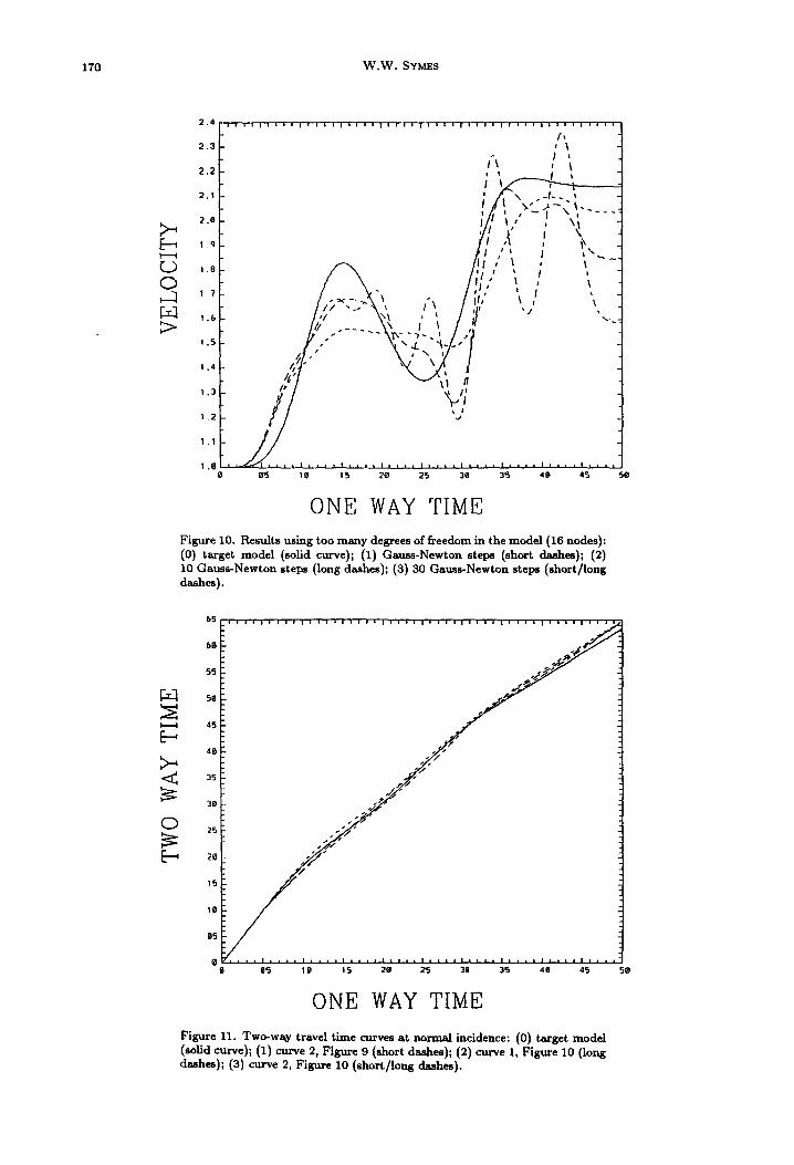
ONE WAY TIME Figure 10. Results using too many degrees of freedom in the model (16 nodes): (0) target model (solid curve); (1) Gauss-Newton steps (short dashes); (2) 10 Gauss-Newton steps (long dashes); (3) 30 Gauss-Newton steps (short/long dashes).

[-~

<~

0

b~ I I l , I , I l l I I I I I I I I I ' I l l l l l . l l l l l l I I | 1 l l l l l l l l l l l I I

6O

55

5O

45

4O

35

3e

25

~e

15

I 0

e5

e ' t i l l I e l I z ' 1 e l a l ' l I n a a l l l l a l a i n t ' I I I ' a I t l l l l I n I I

O gS 1 o 15 20 25 3i 3S 49 45 50

ONE WAY TIME

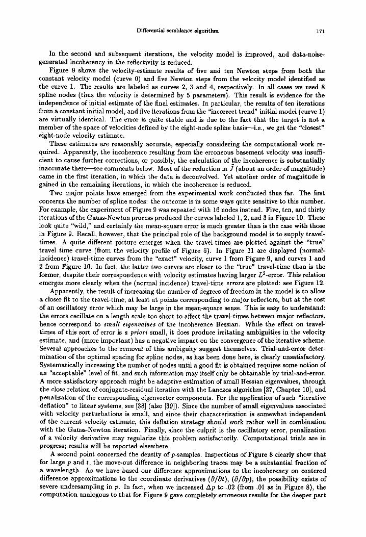
Figure 11. Two-way travel time curves at normal incidence: (0) target model (solid curve); (1) curve 2, Figure 9 (short dashes); (2) curve 1, Figure 10 (long dashes); (3) curve 2, Figure 10 (short/long dashes).


In the second and subsequent iterations, the velocity model is improved, and data-noise- generated incoherency in the reflectivity is reduced.

Figure 9 shows the velocity-estimate results of five and ten Newton steps from both the constant velocity model (curve 0) and five Newton steps from the velocity model identified as the curve 1. The results are labeled as curves 2, 3 and 4, respectively. In all cases we used 8 spline nodes (thus the velocity is determined by 5 parameters). This result is evidence for the independence of initial estimate of the final estimates. In particular, the results of ten iterations from a constant initial model, and five iterations from the "incorrect trend" initial model (curve 1) are virtually identical. The error is quite stable and is due to the fact that the target is not a member of the space of velocities defined by the eight-node spline basis--i.e., we get the "closest" eight-node velocity estimate.

These estimates are reasonably accurate, especially considering the computational work required. Apparently, the incoherence resulting from the erroneous basement velocity was insuffi- cient to cause further corrections, or possibly, the calculation of the incoherence is substantially inaccurate there---see comments below. Most of the reduction in J (about an order of magnitude) came in the first iteration, in which the data is deconvolved. Yet another order of magnitude is gained in the remaining iterations, in which the incoherence is reduced.

Two major points have emerged from the experimental work conducted thus far. The first concerns the number of spline nodes: the outcome is in some ways quite sensitive to this number. For example, the experiment of Figure 9 was repeated with 16 nodes instead. Five, ten, and thirty iterations of the Gauss-Newton process produced the curves labeled 1, 2, and 3 in Figure 10. These look quite "wild," and certainly the mean-square error is much greater than is the case with those in Figure 9. Recall, however, that the principal role of the background model is to supply travel- times. A quite different picture emerges when the travel-times are plotted against the "true" travel time curve (from the velocity profile of Figure 6). In Figure 11 are displayed (normal- incidence) travel-time curves from the "exact" velocity, curve 1 from Figure 9, and curves 1 and 2 from Figure 10. In fact, the latter two curves are closer to the "true" travel-time than is the former, despite their correspondence with velocity estimates having larger L2-error. This relation emerges more clearly when the (normal incidence) travel-time errors are plotted: see Figure 12.

Apparently, the result of increasing the number of degrees of freedom in the model is to Mlow a closer fit to the travel-time, at least at points corresponding to major reflectors, but at the cost of an oscillatory error which may be large in the mean-square sense. This is easy to understand: the errors oscillate on a length scale too short to affect the travel-times between major reflectors, hence correspond to small eigenvalues of the incoherence Hessian. While the effect on travel- times of this sort of error is a priori small, it does produce irritating ambiguities in the velocity estimate, and (more important) has a negative impact on the convergence of the iterative scheme. Several approaches to the removal of this ambiguity suggest themselves. Trial-and-error deter- mination of the optimal spacing for spline nodes, as has been done here, is clearly unsatisfactory. Systematically increasing the number of nodes until a good fit is obtained requires some notion of an "acceptable" level of fit, and such information may itself only be obtainable by trial-and-error. A more satisfactory approach might be adaptive estimation of small Hessian eigenvalues, through the close relation of conjugate-residual iteration with the Lanczos algorithm [37, Chapter 10], and penalization of the corresponding eigenvector components. For the application of such "iterative deflation" to linear systems, see [38] (also [39]). Since the number of small eigenvalues associated with velocity perturbations is small, and since their characterization is somewhat independent of the current velocity estimate, this deflation strategy should work rather well in combination with the Gauss-Newton iteration. Finally, since the culprit is the oscillatory error, penalization of a velocity derivative may regularize this problem satisfactorily. Computational trials are in progress; results will be reported elsewhere.

A second point concerned the density of p-samples. Inspections of Figure 8 clearly show that for large p and t, the move-out difference in neighboring traces may be a substantial fraction of a wavelength. As we have based our difference approximations to the incoherency on centered difference approximations to the coordinate derivatives (O/Ot), (O/Op), the possibility exists of severe undersampling in p. In fact, when we increased Ap to .02 (from .01 as in Figure 8), the computation analogous to that for Figure 9 gave completely erroneous results for the deeper part

172 W.W. SYMES

F-~

[._.,

0

E--

B--+ I - - - I

r.3 c3

ft.1 >

. i p l g

. e B B

• g o t '

.g~14

• 05~2

O

- , B 0 2

- . g~14

- gob

- + 6 0 0

- . O l l a

- . g l : ~

- 0 1 4

- . 0 1 b

l I I | l l i t I , ~ q l I I I I I I I I I l l | I I I I I I I I I | I I I I I I I I I I I I I I

/ \ \ / \ / , ' , \ / X

I / ", \ / k ", \ / X

4+ , \ / I

X P , - , I

/ ', ,," ,X

I , , . I . l , l l l , , . l , , , l l . . , , I i , , , l , l , l l , . l , l l t i l l i l l ,

¢q5 1 0 1 5 ~ip 2 5 3ip 3 5 4 0 4 ~ 5 ~

ONE WAY TIME

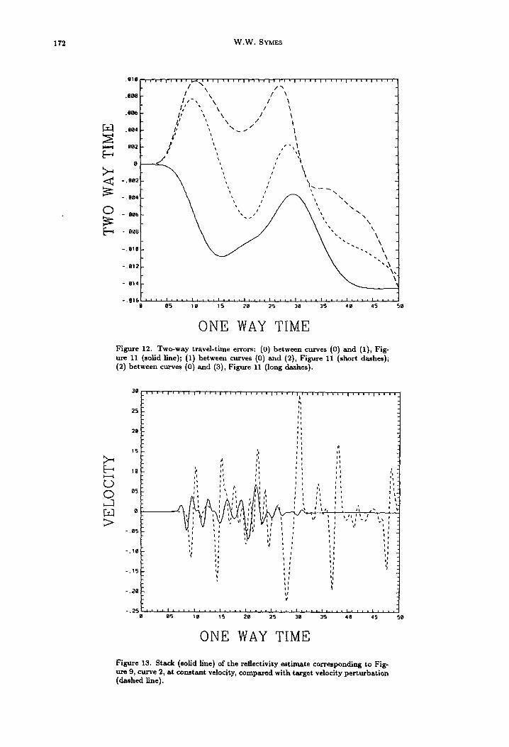
Figure 12. Two-way traveJ-time errors: (0) between curves (0) and (1), Fig- ure 11 (solid line); (1) between curves (0) and (2), Figure 11 (short dashes); (2) between curves (0) and (3), Figure 11 (long dashes).

30

25

20

tS

10

05

0

-+05

- . 1 0

- . 1 5

- . ~ 0

- . 25

l l l l ' ~ l l l l l l l l l l l l l l l l l l l | l l l l l l l l l l l l l l l l l l l l l l I l

I t I I I I

II I I I I I t I I s I

i I

Ii I II I I I I i

II I t I I ~ I I I , , , , ,. ,~, ,',

I r I I I I I I I I I t ~I i I i I

I i f +I " I I

i I | I t +

I i i " ~1 i I 11 I + !

+ I I '

I I t l I I I I |

II i l I I

11 I I I

i i , i I I i i i I I I I i i i i i i i i i i i i i i i l | l l l l l l , , , l l , , l l l l I i

0 5 1 El ~ 5 2 0 2 5 3Q 3 5 4 e 4 5

1 I I l I I i t

S iP

ONE WAY TIME

Figure 13. Stack (solid llne) of the reflectivity estimate corresponding to Fig- ure 9, curve 2, at constant velocity, compared with target velocity perturbation (dashed line).


E~

0 0

>

30

25

• 20

. 15

. 19

• 05

0

- . e5

* . 10

- . 15

- . 20

- . 25

I I I t I I l I I I I I 111 I I I I I I I I I I I I I I l l l l I I I I I I I I I I I I I I I ,

I t I I I t I I I I I I

I I I

-h

i I I I I

i I I I i I

I t I I t I I ,

, ,:! ,,

I I I i e l t l

I I | I i i t l I ¢

l ! I : i , i t ,

I ! I

• L s t t I ~ l

I I

! I I I I I | | t I | 1 I# l |

I

, , | , | 1 * * l I , a * e l , * * , I , * * * | i i l I I , , s | I , I * , I , l * ' J * , * J

95 1 g 15 20 25 3g 35 40 45 50

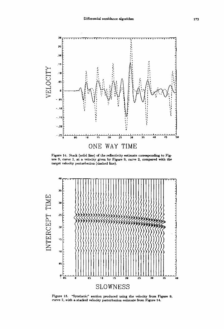
ONE WAY TIME Figure 14. Stack (solid line) of the reflectivity estimate corresponding to Fig- ure 9, curve 2, at a velocity given by Figure 9, curve 2, compared with the target velocity perturbation (dashed line).

49

35

3a

E-~ 25

~-1 15 E -

Z

e - 05 0 95 10 15 2B 25 30 35 40

SLOWNESS Figure 15. "Synthetic" section produced using the velocity from Figure 9, curve 2, with a stacked velocity perturbation estimate from Figure 14.

174 W . W . SYME$

40 , , , ,

L~

35

30

25

20

15

I

- 05 05 le 15 20 25

SLOWNESS

Figure 16. Difference of Figures 15 and 8.

39 35 40

of the velocity profile, apparently because the part of the incoherency due to deeper reflectors was grossly underestimated. We suspect that the residual inaccuracy in the deeper parts of the curves in Figure 9 is due to a milder version of the same effect.

Besides finer sampling, methods to overcome errors in incoherency due to undersampling include higher-order difference formulas and difference formulas better adapted to the move-out. Indeed, low-order differences along even a crude approximation to the correct move-out curve should produce better results at coarser sampling than the coordinate derivatives used in our present code. These ideas are also under investigation.

It might be objected that, while the output includes an estimate of the travel-time reflectivity section r(t,p), no estimate of the corresponding velocity perturbation er(z) is provided. The final refleetivity is not necessarily entirely coherent, and so does not correspond to any er(Z), strictly speaking. Nonetheless, an estimate may be produced by stacking r(t, p) on the basis of equation (5), i.e.,

or(z) [p"" ,~ dp v-~2(z, p) r(r(z, p), p). Pmax J 0

This output might truly be regarded as the final image produced by an iterative before-stack migration, specialized to constant-density acoustics.

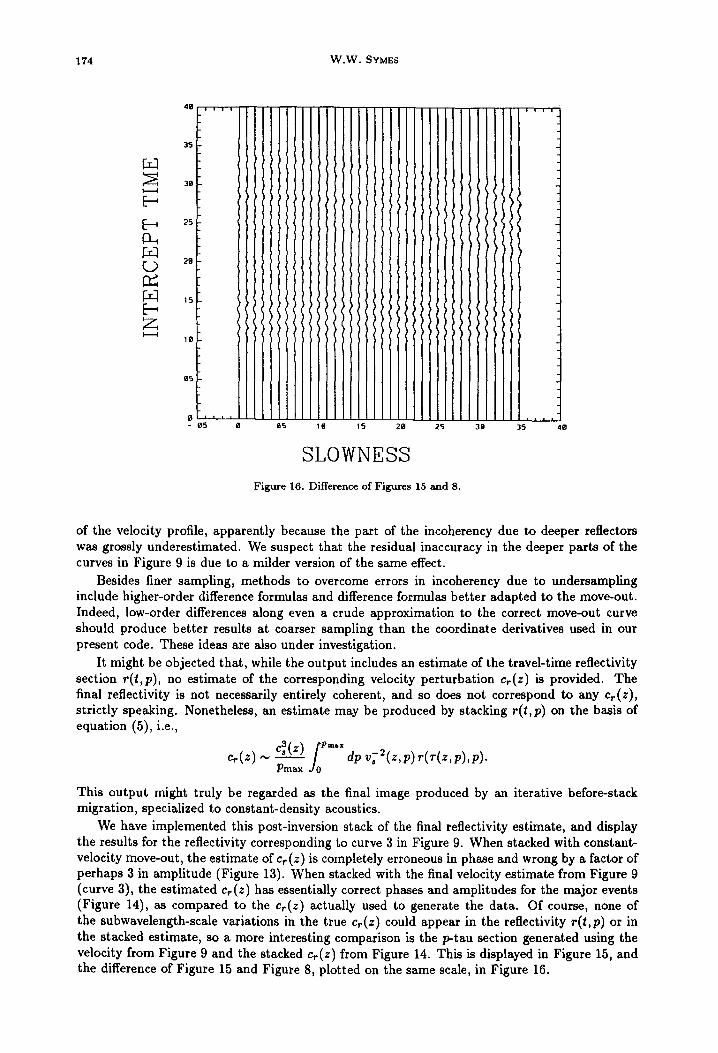
We have implemented this post-inversion stack of the final reflectivity estimate, and display the results for the reflectivity corresponding to curve 3 in Figure 9. When stacked with constant- velocity move-out, the estimate of cr (z) is completely erroneous in phase and wrong by a factor of perhaps 3 in amplitude (Figure 13). When stacked with the final velocity estimate from Figure 9 (curve 3), the estimated cr (z) has essentially correct phases and amplitudes for the major events (Figure 14), as compared to the cr(z) actually used to generate the data. Of course, none of the subwavelength-scale variations in the true cr(z) could appear in the reflectivity r(t,p) or in the stacked estimate, so a more interesting comparison is the p-tau section generated using the velocity from Figure 9 and the stacked cr(z) from Figure 14. This is displayed in Figure 15, and the difference of Figure 15 and Figure 8, plotted on the same scale, in Figure 16.

176 W.W, SYMES

REFERENCES

1. A. Tarantola, A strategy for nonlinear elastic inversion of seismic reflection data, Geophysics 51, 1893-1903 (1986).

2. O. Gauthier, A. Tarantola and J. Virieux, Two-dimensional nonlinear inversion of seismic waveforms, Geo- physics 51, 1387-1403 (1986).

3. Mcaulay, Prestack inversion with plane-layer point source modeling, Geophysics 50, 77-89 (1985). 4. P. Morn, Nonlinear 2-D elastic inversion of multi-offset seismic data, Expanded abstract, 56th Annual In-

ternational Meeting, Society o] Exploration Geophysicists, Houston, pp. 533-537 (1986); also, Geophysics, 52 .

5. P. Kolb, F. Collino and P. Lailly, Prestack inversion of a 1D medium, Proe. IEEE 74, pp. 498-506 (1986). 6. L. Lines and S. Treitel, A review of least-squares inversion and its application to geophysical problems,

Geophysical Prospecting 32,159-186 (1984). 7. A. Bamberger, G. Chavent, C. Hereon and P. Lailly, Inversion of normal incidence seismograms, Geophysics

47, 757-770 (1982). 8. K. Bube, D.B. Jovanovich, R.T. Kangan, J.R. Resnick, R.T. Shuey and D.A. Spindler, WeU-determined and

poorly determined features in seismic reflection tomography: Part II, 55th Annual Meeting, SEG, Washington, DC, (1985).

9. R. Bording, A. Gersztenkorn, L. Lines, J. Scales and S. Treitel, Applications of Seismic Traveltime Tomogra- phy, Geophys. J. Roy. Astr. Soc. 90, 285-304, (1987).

10. L. Ikel]e, J. Diet and A. Tarantola, Linearized inversion of multioffset seismic data in the omega-k domain: Depth-dependent reference medium, Geophysics 53, 50-64 (1988).

11. J.K. Cohen and N. Bleisteln, Velocity inversion procedure for acoustic waves, Geophysics 44, 1077-1085 (1979).

12. R. Clayton and R. Stolt, A Born-WKBJ inversion method for acoustic reflection data, Geophysics 46, 1559- 1567 (1981).

13. G. Beylkin, Imaging of discontinuities in the inverse scattering problem by inversion of a causal generalized Radon transform, J. Math. Phys. 26, 99-108 (1985).

14. L. Lines, A. Schultz and S. Treitel, Cooperative inversion of geophysical data, Geophysics 53, 8-20 (1988). 15. Y. Hadjee and F. Collino, A geometrical approach to the apriori study of the 1-D inverse problem, (IFP

preprint), (1988).

16. F. Santosa and W. Symes, An analysis of least-squares velocity inversion, Geophysical Monograph 4, Society of Exploration Geophysicists, Tulsa, (1989).

17. G. Canadas and P. Kolb, Least-squares inversion of prestack data: simultaneous identification of density and velocity of stratified media, Expanded Abstract, 56th Annual International Meeting, Society of E~:ploration Geophysicists, Houston, pp. 604-607 (1986).

18. P. Lailly, Migration methods: Partial but efficient solutions to the seismic inverse problem, In Inverse Problems o] Acoustic and Elastic Waves, Santosa et al., Eds., SIAM, Philadelphia, 182-214, (1984).

19. P. Morn, Nonlinear 2-D elastic inversion of real data, Expanded abstract, 57th Annual International Meeting, Society o] E~:ploration Geophysicists, New Orleans, pp. 430-432 (1987).

20. A. Tarantola, The seismic reflection inverse problem, In Inverse Problems o.[ Acoustic and Elastic Waves, Santosa et aL, Eds., SIAM, Philadelphia, (1984).

21. G. Beylkin and R. Burridge, Linearized inverse scattering problems of acoustics and elasticity, E~:panded Abstract, 57th Annual International Meeting, Society o] E~:ploration Geophysicists, pp. 747-749, New Orleans, (1987).

22. S. Spratt, Effect of normal moveout errors on amplitude versus offset-derived shear reflectivity, Expanded Abstract, 57th Annual International Meeting, Society of Exploration Geophysicists, New Orleans, pp. 634- 637 (1987).

23. W. Symes, Stability and instability results for inverse problems in several-dimensional wave propagation, In Computing Methods in Applied Science and Engineering VI, R. Glowinski and J.-L. Lions, Eds., North- Holland, (1985).

24. W. Symes, Velocity inversion by coherency optimization, Technical Report 88-4, Department of Mathematical Sciences, Rice University, Houston, TX, (1988).

25. W. Symes, Velocity inversion: A case study in infinlte-dimensional optimization, Math. Prog. 48, 71-102 (1990).

26. W. Symes, Non-interactive estimation of the Marmousi velocity model by differential semblance optimization: Initial trials, In The Marmousi Experience: Proceedings of the EAEG Workshop on Practical Aspects of Inversion, (G. Grau and R. Versteeg, Eds.), pp. 125-138, EAEG, The Hague, (1991).

27. W. Symes, Velocity inversion: A model problem from reflection seismology, SIAM J. Math. A nal., 22,680-716, (1991).

28. W. Symes and J. Carazzone, Velocity inversion by coherency optimization, Technical Report 89-8, Depart- ment of Mathematical Sciences, Rice University, Houston, TX, (1989); to appear in Proe. of Workshop in Geophysical Inversion, J.B. Bednar, Ed., SIAM.


29. W. Symes and J. CaraT.zone, Velocity inversion by differential semblance optimization, Geophysics 56, 654- 663, (1991).

30. A.H. Kleyn, Seismic Reflection Interpretation, Applied Science Publishers, New York, (1983). 31. P. Fowler, Migration velocity analysis by optimization: Linear theory, Expanded A~stract, 56th Annual In-

ternational Meeting, Society of Exploration Geophysicists, Houston, pp. 660--662 (1986). 32. W. Symes, Stability properties for the velocity inversion problem, In Proc. oJ ConJerence on Set#sic Ezpio-

ration and Reservoir Modeling, W. Fitzgibbon, Ed., Philadelphia, SIAM (1986). 33. A. Tarantola and B. Vailette, Inverse problems: Quest for information, J. Geophysics 50, 159-170 (1982). 34. H. Brysk and D. McCowan, A slant-stack procedure for point-source data, Geophysics 51, 1370-1386 (1986). 35. J.E. Dennis Jr. and R.B. Schnabel, Numerical Methods .for Unconstrained Optimization and Nonlinear Equa-

tions, Prentice-Hall, Englewood Cliffs, (1983). 36. T. Steihaug, Quasi-Newton methods for large-scale nonlinear problems, Ph.D. Thesis, Yale, (1981). 37. G. Golub and C. Van Loan, Matrix Computations, The Johns Hopkins University Press, Baltimore, (1983). 38. T. Chan, Deflated Lanczos procedures for solving nearly singular linear systems, Research Report

YALEU/DCS/RR-4O3, Department of Computer Science, Yale University, (1985). 39. J. Meza and W. Symes, Deflated Krylov subspace methods for nearly singular linear systems, Technical Report

87-3, Department of Mathematical Sciences, Rice University, Houston, TX, (1987). 40. P. Sacks and W. Symes, Recovery of the elastic parameters of a layered half-space, Geophys. J. Roy. Astr.

Soc. 68, 593-620 (1987).

A P P E N D I X

Computation o.f a Derivative

This appendix details the calculation of the derivative of the incoherency

W[c,r] = [:---p(v-2ro,)] o ( = - 2 p r + [v-2:---~(ro-)] o(;

(o, o,f,o j = - 2 r r + ~ - ~ ° ¢ ~ - P ~ J o

in which have been used the identities

"-2=-2P' ~ = P ' ~ ' ~=-PJo " "

Clearly, ~W = 6cW + 6rW,

with 6,w = W[c, 6r].

On the other hand, an easy calculation shows that

(A.1)

o 6c

So, from the second line in (A.I),

f' r±( , .o , ) ] o, ,., a~W = 6(u -2o:.) Lap at Jo (A,2)

[ /o ] [/o 6c 1 8c ~ v - 2 8r = -2 ~ + ~ c ~ o( ( ,or) o ( - p ^~c+~ -2 ^8 o ¢ ~ .

An alternate form of (A.2) follows from the identity

/ o ( / . ' ) / o ' I' < ~ = ~ (v o ~)~ 8(~ o 6 = 2 (,,oOa(~oO=2 0o~.

So, using the notation

( I" Q8c=~(~o¢)o,=^ 3 6c+~ c3)

the first line in (A.2) may be re-written

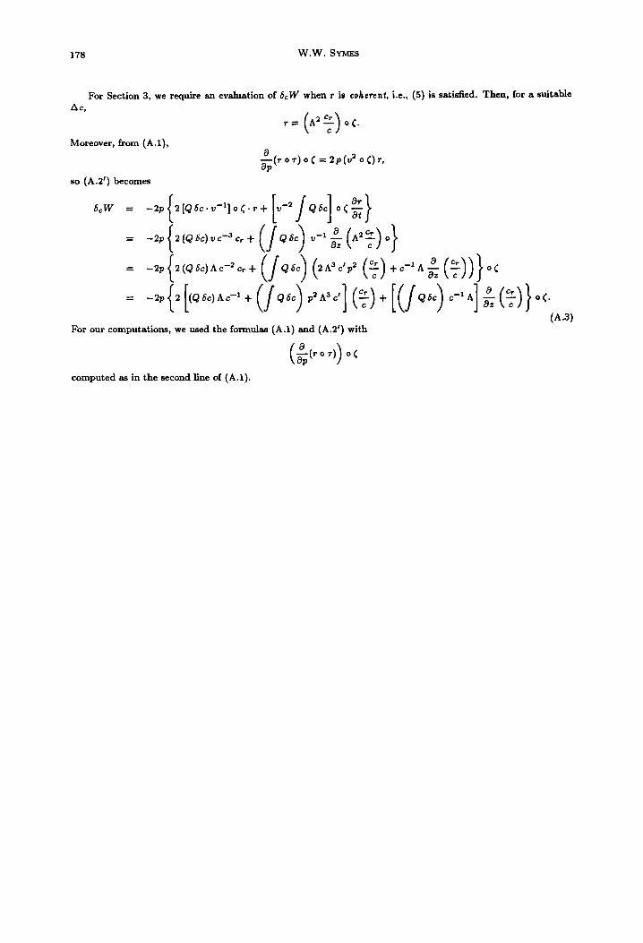
178 W.W. SYMES

For Section 3, we require an evaluation of &W when r is coherent, i.e., (5) is satisfied. Then, for a suitable

Ac,

Moreover, from (A.l),

r= ( 1 A2 cp o c.

c

$(ToT)0[=2p(POC)r,

so (A.2’) becomes

6,W = -2p 2[Q6c.v-‘]oC.T+ 1

[u-2JQ6c] oCa>

= -2p 2(C36C)VC {

-SC,+ (JQ,sc) v-1; (e) o}

= -2p 2(Q6c)Ac4cr+ (Jwc) (2i~cy (5) +c-~; (s))} oc 1

= -2p{2[(~~c)n.-1+(J~sc)p2A3c~] (~)+[(Jwc) c-l~]$(%)}e.

(A.3) For our computations, we used the formulas (A.l) and (A.2’) with

(;(--I) oc computed as in the second line of (A.l).

Documents

A DIFFERENTIAL SEMBLANCE ALGORITHM FOR THE … · faithfully reflect the physics of the reflection seismology experiment, at least at the level of detail desired in the subsurface