A differential game in three dimensions: The aerial dogfight scenario

Dynamics and Control 2, 161-200 (1992) © 1992 Kluwer Academic Publishers, Boston. Manufactured in The Netherlands.

A Differential Game in Three Dimensions: The Aerial Dogfight Scenario

NIGEL GREENWOOD Mathematics Department, University of Queensland, St. Lucia, Q4067, Australia

Received June 28, 1990; revised July 18, 1991 Editor: M. Ardema

Abstract. In this article, an aerial dogfight in three dimensions between two aircraft was modeled, with each aircraft having combined qualitative objectives of capture with avoidance. A spherical polar-coordinate system was devised to describe the system. From a standard point-mass model of aircraft dynamics for three-dimensional flight, a kinematic model was derived, with its corresponding controls for each aircraft. This kinematic model was then used, assuming bang-bang control functions for each aircraft, in order to determine a map of the game. A technique of trajectory dissection was introduced, whereby the airplane loci were decomposed in terms of regions of zero-level and saturation-level control values, and controllable and winning regions were determined for each aircraft using a Liapunov-function approach, the winning regions being calculated using the Getz-Leitmann theorem. A map of the game was constructed, and the barrier was found to be nonvoid. The concept of the posthumous mutual-kill strategy was introduced.

1. Introduction

1.1. On combat games

There exists in literature a multitude of papers which address themselves to the issue of air combat as modeled by a two-player zero-sum pursuit-evasion differential game where the roles of pursuer and evader are predetermined and fixed. Based upon this assumption, these papers then consider the problem of determining either precise t ime-optimal player strategies or approximations to these in order to resolve the ensuing conflict. A particular example of such a paper, which we shall further invoke, is Rajan and Ardema [18].

However, in a genuine air combat scenario, particularly between armed aircraft of similar capabilities, the issue of role determination is an open question. The arbitrary a priori

assignation of roles to the players concerned is unrealistic, particularly considering that a particular player may alternate between aggressive and defensive maneuvers several times during a skirmish. Because of this, the above formulation becomes of l imited use. This problem of rote determination is addressed in a number of ways in a variety of papers, in part icular by Ardema, Heymann, and Rajan [1], [2], and in a more tangible model- dependent way by Peng and Vincent [41, Merz [9], and Davidovitz and Shinar [25].

In the case of the latter three papers cited, the calculated criteria for role decision are derived from the specific geometries of the firing envelopes of the weapon systems used by the fighter aircraft, since these firing envelopes become the target sets for the game. For example, the weapons systems used in [4] and [9] are forward-firing guns or missiles,

162 N.J.C. GREENWOOD

with cone-shaped firing envelopes. In [25] the weapon systems are all-aspect guided missiles with firing envelopes described by eccentric circles. In this last paper, the other salient feature in the role decision lies in the asymmetry of the duelling airplanes, one being of the Hawker Harrier type, the other being a faster, less maneuverable conventional type.

In [1] and [2], the authors of those papers discuss various frameworks through which to perceive the air combat problem, namely, via 1) the single pursuit-evasion formulation with roles fixed, 2) the superposition of two pursuit-evasion scenarios, with the roles alter- hated, and 3) the two-target game concept, as per Getz and Leitmann [17]. Criticisms of each of these frameworks are presented in this article, based on perceived shortcomings in role resolution. The authors also postulate a fourth formulation, namely, the 6-combat game based on min-max optimization of cost functionals.

Skowronski and Stonier [22] formalize the superposition of two semigames and adopt the two-target game concept (point 3 above) from [16], combining it with the concept of single pursuit-evasion (point t) to analyze kinematic pursuit-evasion between inenialess objects in the vertical plane. Their analysis is in terms of the map of the game of kind in the sense used by Isaacs [21]. To draw the map, they use a theorem from [16] and a technique of superimposing two alternate pursuer-evader configurations in the plane.

The present article draws its inspiration from [22]. Despite the existence already of some highly sophisticated papers discussing pursuit-evasion based on point-mass aircraft dynamics in three-dimensional flight and the calculation of optimal strategies, such as that of Menon [24], computation of these strategies appears complex and time consuming. Even if such computations become viable in a real-time sense on board an aircraft, as is suggested in Menon [26], there still exist those criticisms already made regarding the actual validity of pursuit-evasion models in aerial conflict. The existance of such objections led to this formulation of air conflict in three dimensions, and its analysis in terms of the game of kind.

We contend that given the problems associated with real-time calculation of time-optimal strategies based on pursuit-evasion and interception, not to mention those to do with the role assignation, a completely different approach based on the game of kind is desirable. The motivation is to ultimately create a tool that will be useful to a pilot during real-time aerial combat, whereby the pilot is advised as to the existence and location of winning regions, mutual kill regions, and barriers. The principal objective here is the determination of these regions, not the computation of strategies.

1.2. The game scenario

To this end, this article will use a superimposed pair of two-target semigames. In each semigame there exists an inherent asymmetry in the nature of player target sets, although both players in each semigame have combined qualitative objectives. The technique of alter- nating two configurations as per [22] will be used along with the Getz-Leitmann theorem in order to determine the various regions of the game.

We have two mutually hostile fighter aircraft, assumed identical, maneuvering in three dimensions. We assume that we are dealing with intermediate-range combat, using omnidirectional missiles instead of beam weapons. In reality, these missiles would not be completely reliable, so either aircraft could enter within range of the other without a guarantee

A DIFFERENTIAL GAME IN THREE DIMENSIONS: THE AERIAL DOGFIGHT SCENARIO 163

of destruction. For this reason, if both aircraft are armed, then role determination of pursuit or evasion cannot be strictly resolved by superior missile range. Furthermore, each aircraft has taken off from a friendly airstrip. We assume each airstrip is protected by ground- to-air defenses, which are accurate to a certain range from the ground. This provides an option of escape.

Throughout this article, continual use will be made of the terms pursuer and evader. It should be noted, however, that each semigame will actually be two-target in nature.

In each semigame, there will exist exactly one player whose aircraft is carrying the omnidirectional air-to-air missile system. The other player's aircraft will be unarmed. For ease of terminology, the armed aircraft will be designated the pursuer and the unarmed aircraft will be the evader. The player of the evader will be designated player one, and the player of the pursuer will be designated player two. The evading aircraft possesses an airstrip equipped with a ground-to-air defense system. The pursuing aircraft has no such airstrip.

The airborne missiles of the pursuer are of range pp. For the purposes of this model, we will assume that all missile systems are completely reliable. The "kill" region around the pursuer's aircraft, dictated by missile range, is represented as a sphere in actual space of radius Pc, with the pursuer's aircraft at the center of the sphere. Violation of this sphere at any time by the evader results in the instantaneous destruction of the evader. The actual controls for the missile responsible are ignored, as are aerodynamical effects and weight differences upon the pursuer due to launch.

Furthermore, the evader has a hemisphere of safety centered at some point on the ground, representing the ground-to-air defenses of his airstrip. This point is taken to be the origin O of the coordinate system for the game. The hemisphere is of radius p~, and violation of this hemisphere results in the instantaneous destruction of the pursuer in an analogous fashion. This provides the option of "mutual kill" in the game.

1.3. Objectives

The combined objectives of the pursuer P are to rendezvous with or capture the evader E at time T~ < oo (where his target region for rendezvous in state space is the region r2 for which the pursuer-evader distance PE < pp) while avoiding his antitarget T~ (which is the region for which OP <_ Pe) for t < T~.

Similarly, the combined objectives for the evader are to be captured by the target 7-1, where 7 1 ~ 7"~, at some time Tb < ~ , while avoiding his antitarget 7"~', where 7"~ = 7"2, for time t < Tb.

We assume that pe, pp >> aircraft dimensions, and complete information for both players. The game terminates when either or both players are destroyed.

2. Dynamic and kinematic equations: controls

2.1. System dynamics

In this article, we shall be predominantly using kinematics, rather than dynamics. This is because a kinematic model has much greater simplicity than the corresponding dynamic


/ J

O'

/

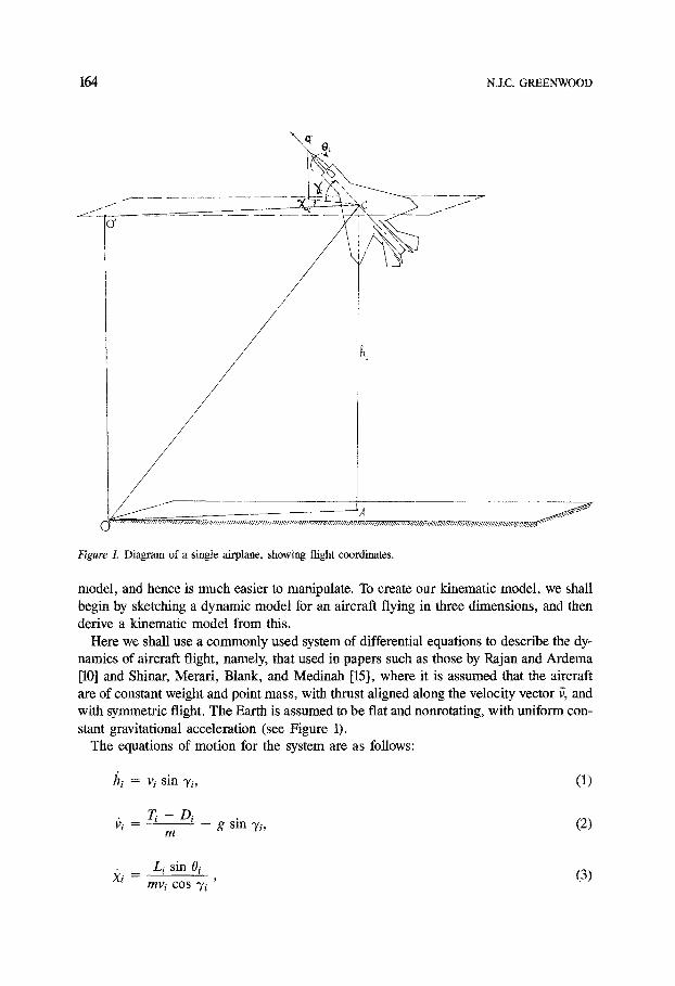
Figure L Diagram of a single airplane, showing flight coordinates.

model, and hence is much easier to manipulate. To create our kinematic model, we shall begin by sketching a dynamic model for an aircraft flying in three dimensions, and then derive a kinematic model from this.

Here we shall use a commonly used system of differential equations to describe the dynamics of aircraft flight, namely, that used in papers such as those by Rajan and Ardema [10] and Shinar, Merari, Blank, and Medinah [15], where it is assumed that the aircraft are of constant weight and point mass, with thrust aligned along the velocity vector ~, and with symmetric flight. The Earth is assumed to be flat and nonrotating, with uniform constant gravitational acceleration (see Figure 1).

The equations of motion for the system are as follows:

hi : vi s i n ~ i , (1)

vi Ti - Di - g sin 7i, (2) m

Xi - Li sin Oi (3) m v i cos "/i '


g/i --

where

L/COS 0 i g cos y~ mv/ v/

(4)

hi is the vi is the Xi is the "Yi is the m is the ai is the Oi is the 7r i is the

altitude for the ith aircraft, aircraft speed, horizontal flight-path angle, vertical flight-path angle, airplane mass, assumed identical for both aircraft, angle of attack, bank angle, throttle.

Note here that Equation 3 describes the rate of change of yaw, as per [10] and a fixed Cartesian system. For clarity in discussing dynamics, the extra term due to the use of the origin--aeroplane polar axis as the zero axis (illustrated in Figure 1) in this article is a method in Sections 2.1 and 2.2.

In Equations (2) through (4), the aerodynamical forces T/, L/, D i a r e defined as follows:

zij~

p(hi)v2SCLa(Mi)oti Li(hi' vi' °ti) = 2 (5)

Thrust

T/(Tfi, hi, vi) = 7r i TM(hi, Mi) (6)

Drag

p(hi)v2 S Oi(hi, vi, ai) = [CDo(Mi) + rl(Mi)C~(Mi)a 2] 2 (7)

where

E i is the ith aircraft's specific energy, M i is the ith aircraft's Mach number, p(hi) is the atmospheric density, CL~ is the lift coefficient slope w.r.t, angle of attack, S is the airplane's wing reference area, TM is the maximum thrust available, CDo is the base drag coefficient,

is the efficiency factor.

Note that we assume here that thrust is a linear function of throttle. We split the drag into two components, namely, the zero-lift and induced-lift components.

166 N J . C . G R E E N W O O D

In a dynamic model, aircraft i has the following control variables:

7ri ( [0, 1] throttle, (8)

o~i ~ [OZm, aM] where et m < 0 < aM, angle of attack, (9)

[0el E [0, OM(Me, hi)] bank angle. (10)

In this article, we shall assume that p(hl) = p(hz). Since we wish this discussion to be kinematic, the first step is to replace the dynamic

control variables (c% Oi, roe) with kinematic control variables. We have chosen the kinematic variables (7i, Xi, i~i) to be suitable replacements. These variables inherit constraints from those of the dynamic controls, namely,

(2 i ~ [Vim , ViM(hi, Mi, Vi)], (1 t)

where i~im <--- 0 < ViM; fen corresponds to drag with zero throttle,

I@et E [0, @eM(hi, Me, v/)], (12)

and

I xi[ E [0, XiM(he, Mi, ve)]. (13)

To understand the precise nature of these constraints, we must look, at the airplane's flight envelope.

2.2. The dynamic flight envelope

The dynamic equations have the following constraints.

Terrain limit

hi>_ 0

Maximum dynamic pressure limit

1 qi = 2 0.5p(hi) " v~ <_ qM

Placard limit

v i <_ Vip(Ei)

Maximum Mach number limit

V i ~--- a ( h i ) ' M M


Aerodynamic load f ac to r

Inil <- nM

Loft ceiling

1 CL~(MI) " O~M" ~ p(hi) " v z " S >- mg

• Lif t l imit

Li(hi, vi, oti) <- rain [CLc~(Mi)OlM ° P(hi)v~S, nMmg]

where

a(hi) is the speed of sound, n i is the aerodynamic load factor, qi is the airplane's dynamic pressure,

and the subscript M denotes the maximum value of these variables. Hillberg and J~mark [5] consider coplanar horizontal pursuit-evasion with a variable-

speed model where the longitudinal acceleration depends on speed, turn rate, and throttle setting. Their model employs the aircraft turn rate and throttle setting as controls. The turn rate for each aircraft is constrained by both structural and stall limits.

The horizontal turn rates Xi are constrained at low speeds by the maximum lift coefficient I CL~ " OtM[, and at high speeds by the structural limit. The threshold between the two limits occurs at the c o m e r speed vie, given by

The stall limit gives

~J 1

where

V i ~ [Vim ,Vic], (14)

g i ~ p(hi) • S " fLu • ot M. 2mg

The structural limit gives

= - - , vi ~ (vic, viM]. (15) I l <- xiM g n? vi

168 NJ.C. GREENWOOD

2.3. System kinematics

In three dimensions, we consider the geometry of the game in terms of the following configurations, both developed in a three-dimensional spherical polar coordinate system, where relative-geometry coordinates are denoted with a prime ..... to distinguish them from the coordinates of the individual aircraft (see Figures 2 and 3).

Xi~ is the relative heading of aircraft i as observed by aircraft j . The Axi ~. angles in this coordinate system are included, since they become significant if we extend this work to include the problem of role determination during the game when forward-firing beam weapons are used to replace the omnidirectional missiles, and hence the conditions of fixed a predetermined roles can be relaxed (see Peng and Vincent [4], Kelley and Lefton [7], and Mertz [9]).

We have the horizontal-plane relative angles obeying the following equations:

AXIr2 -71" --~ X21 ' = -- X12~ (16)

AX;2 = 27r - A X 2 1 , (17)

AX{2 = ¢ ' + X2 -- X1, (18)

r t c o s ~b ~ sin 6 ' = sin(x2 + X~2) R ' cos O ' ' (19)

X21 -- Xlt2 = 7'i" "]- ¢ " "~ X2 -- Xl . (20)

The equations of motion for the relative geometry coordinates in this configuration are

• r t COS q~t

¢ ' = [(x2 + xh) R' cos ¢ ' " cos(x2 + X1'2) + sin(x2 + X/z)~] " - - 1

cos ¢ ' (21)

(Axe2) : ~-]1 + X2 - - X1, (22)

(AXe'z) = xz," - k~, (23)

• R ' cos ~ ' 1 ¢ , " ' ~b' [ ¢ ' cos - ~ sin(x2 + X1'2)] - X2,

X 1 2 - - r ' cos cos(x2 + X{2) (24)

• , _ 1 R ' cos ,I,' ¢ , X2i cos(x2 + X;2) r ' cos 4~' [ ~ / c o s - ~ sin(xz + X~z)] + ¢ - Xl, (25)

/~'(t) = - v l cos Xl cos(2/1 + ¢ ' ) , (26)

vl I sin 71 + cosx1 cos('Yl+ ~ " ) ' t a n q " l , (27) '(t) = ~ ~ ¢,

8 o o i e~

o 8

~2

"7

jJ

--/~

F~

.

..

..

.

~~H

'̀'~.

//Nl~

H#'

/H`~

'i'j]

~lftr

'1ll~

z1Ia

H~I

lzH

(~H

lIa~i

lI~ly

Hg¢

zl~N

IHH

lrH

H¢~

IIll~

iH#I

I/#e1

I(t/u

Hzz

/z#~

z/H

z/ j

Z

t"

© z

o

o t~


, ' AI~1', ' r •

t t x

Figure 3. Diagram of the horizontal projection of the origin-evader-pursuer configuration, as seen from above.

?'(t) = - v 2 cos X~2 cos(y2 + 4)') + vl cos X~I cos(71 + ~b'), (28)

_ 1 , {v2[sin "r2 + cos X~2 cos('r2 + 4~') sin 4)'] '(t) r ' cos

- vl[sin ~/~ + cos X~'l cos('rl + 4)') sin ~ ' ] } , (29)

where

~ JR' cos ~ ' ( ? ' cos ~ ' - r ' ~ ' sin ~ ' )

1 - r ' cos ~ ' ( /~ ' cos i f ' - R ' ~ ' sin ~ ' ) ] R, 2 cos2 ~ , (30)

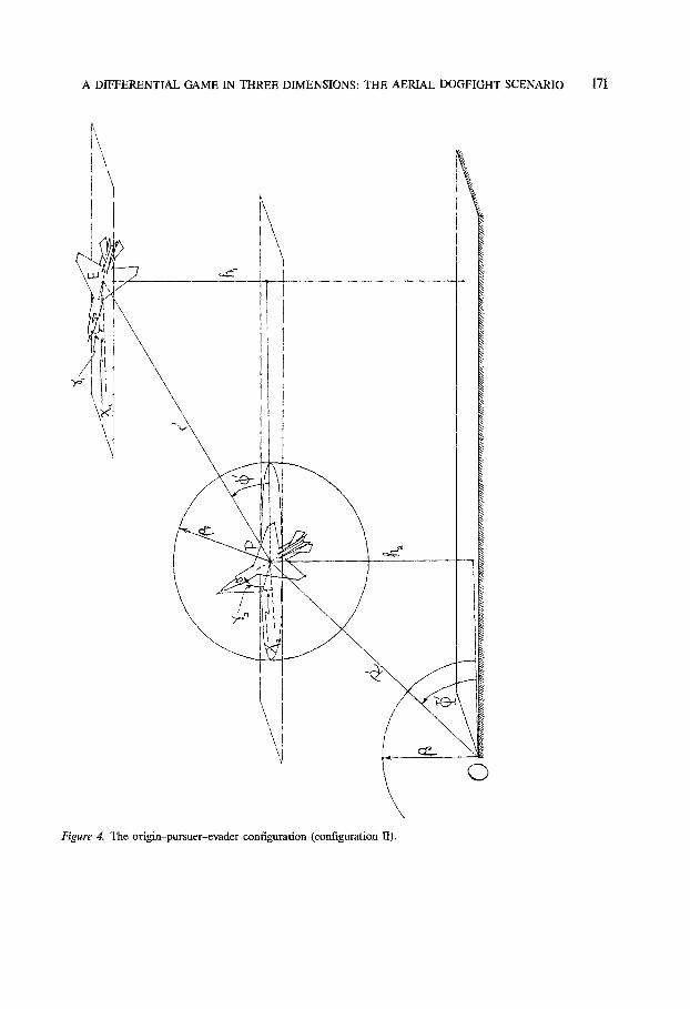
Similarly, by exchanging the positions of pursuer and evader in Figures 2 and 3, we obtain the second relative-geometry configuration, that of origin-pursuer-evader, denoted as configuration II (see Figures 4 and 5).


I\ \

I ,

~', i!l \

I \\

1 I

\

Figure 4. The origin-pursuer-evader configuration (configuration II).

©


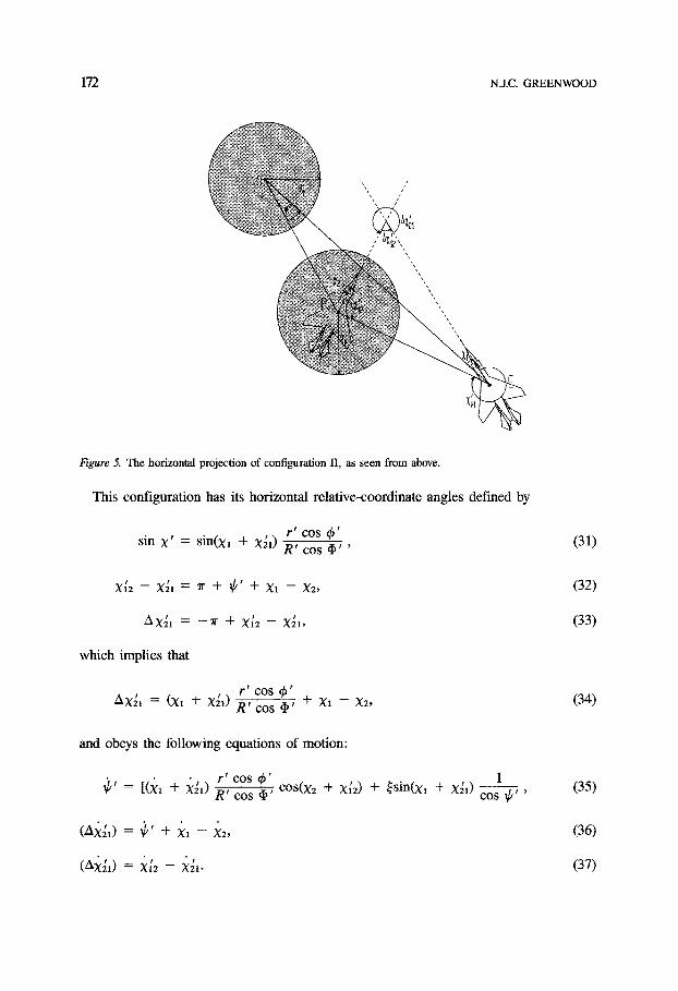
Figure 5. The horizontal projection of configuration II, as seen from above.

This configuration has its horizontal relative-coordinate angles defined by

r t C0S ~P sin X' = sin(x~ + X~I) R' cos 0 ' '

X;2 - X~l = 7r + ¢ ' + X l - X2,

A x21 = - -Tf "~- X;2 -- X21,

which implies that

r ~ COS ~ t

AX~ = (Xt + X~'0 R ' cos ¢ ' + X~ - X2,

and obeys the following equations of motion:

- r ' cos ¢ ' 1 ¢-----7 , ¢ ' = [(~(~ + X~) R ' cos 0 ' cos(x2 + X;2) + ~sin(xl + X~l) cos

( A x ~ I ) = ~ / ' -I- X1 - - X2,

(Axe,) , • = XI2 - - X21"

(31)

(32)

(33)

(34)

(35)

(36)

(37)


Hence,

•, 1 R ' cos ~ ' X12 Cos(x1 -[- X21) r ' cos ¢ '

• R ' cos ~ ' 1 X~t = r ' cos 4~' " cos(x~ + X~I)

where ~ is as defined in Equation (30). Furthermore,

/?'(t) = - v 2 cos X2 cos(3,2 + '~ ' ) ,

[~ ' cos th' - ~ sin(x1 + X~I)] + ~ - X2, (38)

[¢ ' cos X' - ~ sin(x1 - X~I)] - Xl,

'(t) - vz sin "r2 R ' c--~,I~' + cos Xz cos(y2 + ,I~') • tan ,I~'],

t:'(t) = - v l cos X~'l cos('rl + ~b') + v2 cos X;2 cos(y2 + 4~'),

_ 1 '(t) r ' cos q~' {vt[sin "Y1 + cos X~l cosff/x + 4~') sin q~ ']

- v2[sin 3'2 + cos X[2 cos(q~2 + 4 ' ) sin ~b']}.

(39)

(40)

(41)

(42)

(43)

2.4. Set-valued programs and the dissection of trajectories

In order to determine a map of the game, we need simply to consider candidate trajectories for each aircraft issuing from all possible configurations and assess the qualitative behavior of these trajectories. Our concern is to discover the existence of trajectories that exhibit particular forms of behavior, rather than directly proving any sort of global behavior for all trajectories• For this reason we can restrict ourselves to contemplating particular kinds of families of candidate trajectories issuing from all possible configurations, provided these families are not only more amenable to analysis but also possess the required trajectories and have some sort of physical justification. For a more complete discussion of the dynamics of the game, see Section 3•

For our candidates, we will use trajectories employing purely set-valued control programs, switching over a finite set of values in the closed interval between the bounds of the respective controls. All control programs from now on will be assumed bang-bang unless stated otherwise.

We turn our attention first to control programs for vi(t) E [¢m, VM], which is an obviously compact set. ~,, corresponds to drag with zero thrust. I f the aircraft are flying using time- optimal programs in order to attain a minimum-time interception in three dimensions, then their control programs for vi will generally be bang-bang, switching speeds between their "corner speeds" and their maximum speeds (for more details, we refer the reader to Rajan and Ardema [10]). We can decompose such time-optimal interceptions into intervals of hard turning, interspersed by high-speed straight-line dashes.


As such, assuming a three-level bang-bang control for vi, we can now split the trajectories for aircraft i into three sets of disjoint regions, namely, those for which vi = a)M, vi = Vm, and vi = 0. The union of these regions is the entire trajectory, except possibly for a countable set of points. We will scrutinize those trajectory regions for which ')i = 0, i.e., constant-speed sections of the aircraft trajectories. We will ignore the other regions, where vi = f~i M or vi = vim.

Now, in a similar fashion to that used for the fi controls, we split the trajectories of the airplanes into two sets of disjoint regions for each of the two angular controls for each airplane. These correspond to the two possible values for the bang-bang control programs, i.e., the zero-level and the saturation-level control regions.

When analyzing the qualitative behavior of these trajectories using the Getz-Leitmann theorem, we will consider only the zero-level regions for either of the two angular controls and ignore the other regions. In other words, we will use the Getz-Leitmann theorem within the trajectory regions defined by the zero-level control regions for each airplane, in order to establish the qualitative behavior of that particular trajectory.

Hence, for the angular controls,

either Xi(t) = 0 or [Xi(t) l = XiM(hi, ni, v,.)

and

either ~/i(t) = 0 or t+i(t) t = ~YiM(hi, Mi, vi).

Furthermore, given any times tl, t2 where tl < t2, we have

vi(t2) = f t [ 2 vi(r)dr E (0, VIM], (44)

where ViM = min[a(hi) • MM, vie(El)], and

L t2 • xi(t=) = xi(r)dr E [-27r, 2~r],

1

f l t2 " "gi(t2) = yi(r)dr 6 [-27r, 27r]. (45) 1

Hence, vi(-), 3'i('), Xi(') are continuous, piecewise differentiable functions. Therefore, in determining the winning regions for the two players, we can speak of xi(t)

and 7i(t) as their equivalent controls, since the programs for Xi and 3'i translate into equivalent programs of Xi and 7i- Naturally, the equivalent control programs for the speed and these horizontal angles will not be bang-bang. In ignoring the regions of motion for which Xi # O, 3'i # O, we are able to ignore explicit reference to the bank angles 0i.

It is important to note t/ere that we assume Xi) is uncontrollable for player i; i, j E {1, 2}, i ;~ j, since these angles are dictated by how aircraft j observes him, rather than directly by player i's controls. Examination of Equations (20), (21), (32), and (33) should help con- vince the reader of the validity of this assumption.


3. The state representation of the game

3.1. Qualitative objectives: capture with avoidance

We have two mutually hostile players in strict competition within a system described by the vectorial ordinary differential equation

x = f (£ , fi 1, Ft2, t) (46)

where both players influence the state vector through use of their respective controls/i ~, ti 2. The state vector £(t) varies for t >_ to = 0 in a given open, bounded playing set A within the state space ~N, with the control vectors/i i, i = 1, 2 varying in given compact sets U i of control constraints within the spaces of control values ~ri, i = 1, 2, respectively.

The state vector £(t ) = (x i (t) . . . . . XN(t ) ) T varies along the solutions ~(£ o, to,/i 1 (.), ti 2(. ), t) of equation (46), t _ to, where these solutions are defined for some pair of control functions f i ,( .) , ~/z(.) v£o a__ ~(0) ~ A.

The selection of the values Fti(t) i = 1, 2 is done by feedback control programs fii(.) : A - , {all subsets of Ui} , which are generally set-valued functions in order to allow for discontinuities, e.g., for bang-bang control functions. The control value selection is defined by

fii(t) ~ fii(£(t)), t >_ O. (47)

In any two-player competitive game, the objective can be either

1. quantitative--i.e., the players wish to minimize/maximize some cost function F : A ~ ~k or else

2. qualitative--the payoff is an objective property Q(i) in favor of player i of the trajectories of Equation (46) on some Ao c A, Ao # 0.

We ask, "Do these trajectories possess this property?" The answer is either "yes" or "no" Here, we are concerned purely with an analysis of qualitative objectives, namely, capture

with avoidance. Player i {= 1, 2} wishes to run away before being intercepted by player j , {= 2, 1}, and j wishes to intercept i before he runs away. I f we consider the semigame for i, we have Q(i) being "capture of Ti while avoiding z/before capture?' Mathematically, player i has two objectives, namely, he wishes to find a program

/~i(.) : Oh --- A0 -+ {all subsets of U i }

so that 3rE > 0 such that

i (i) (o(£ °, to, t) ~ ri Vt > Tic. = to + tc, = ' for some Ao c A. (ii) ~o(£ °, to, t) E r" Vt < T' C to + t o

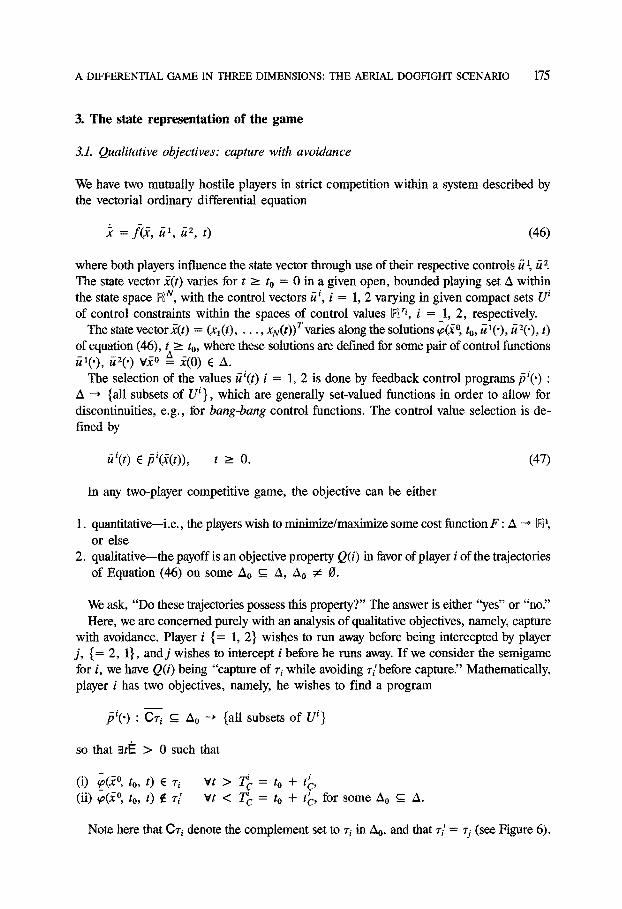
Note here that Ori denote the complement set to zi in Ao, and that r" = rj (see Figure 6).


Figure 6. Diagram of collison with avoidance.

3.2. The map of the game

Now consider the map of the game--in other words, a dissection of some subset Ao c A into sets defined in terms of the attainability of the qualitative objectives of trajectories emanating from Ao. We require nontrivial play for all trajectories emanating from v~ ° E Ao, so we define

Ao = A \ ( r l O r~).

First of all, the dynamics of the game are specified by the so-called contingent equation

x E {3~(07, t, t71, t72) I fii E/3i(x, t)} (48)

with solutions defined on A0. We define

pi A {fii(.) : A --+ all subsets of ui}. (49)

We will now define the concepts of controllability and strong controllability.


Definition 1. The system is i-controllable at (~o, to) for Q(i) iff 3/3,~(') ~ p1,/3,2(.) E p2 such that all of the solution trajectories to

x ~ { ] (~o , to, ~1, n,2) t ~.~ =/3.~(~(t)), ~.2 =/3.:(~(t))}

exhibit Q(i). We call the set of all such yo the region of i-controllability Aiq.

Defnition 2. The system is strongly i-controllable at (yo, to) for Q(i) iff 3/3/0) E pi such that all of the solution trajectories to

-i tT:)l - i = - i - ~s x ~ {f(2o, to, u., u. p',(x(t)), fi q3. j}

exhibit Q(i), regardless of any strategies of player j , j ~ i. We call the set of all such i ° the region of strong i-controllability or the i-winning region A~, and we call/3~(') the winning strategy.

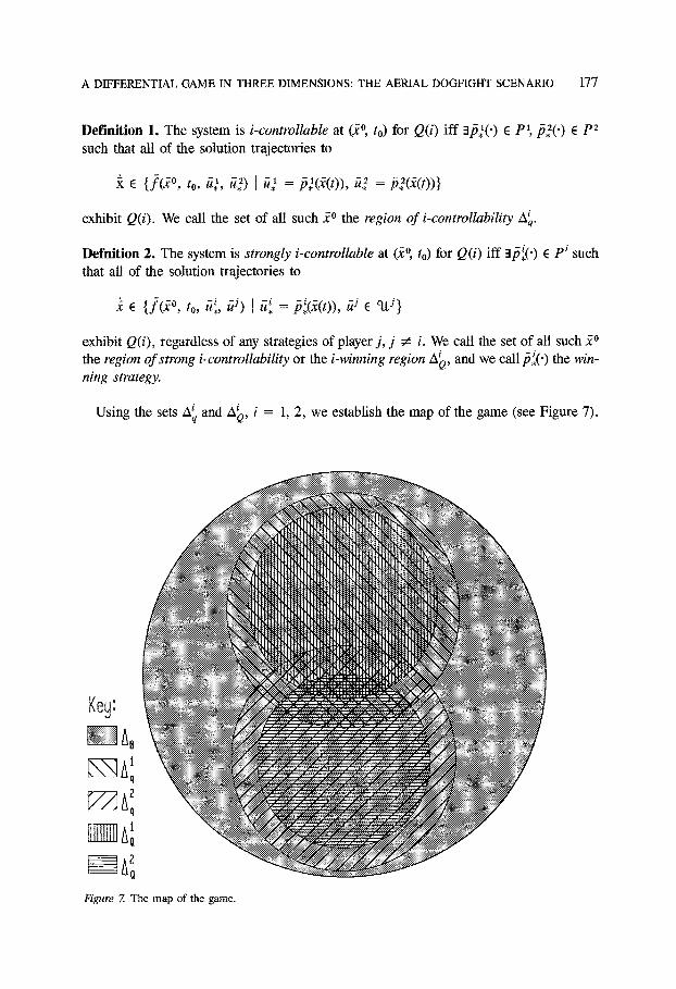
i and A~, i = 1, 2, we establish the map of the game (see Figure 7). Using the sets Aq

Key:

Figure 7. The map of the game.


3. 3. Subsets involved in the map of the game

A~ is the 1-controllable region.

A~ is the 2-controUable region.

An ~ Ao \ (A~ U A~) is the dead zone. A~ c A~ is the 1-winning region. A~ A~ is the 2-winning region.

Wlz A~ N A~ is the mutual kill region. RNGO ~ (A~ C1 A~) \ (A~ U A~) is the region of no guaranteed outcome. D1 A 2 = Aq \ (A~ U A~); player one is guaranteed that a draw strategy exists.

D 2 ~ 1 = Aq \ (A~ U A~); player two is guaranteed that a draw strategy exists.

Note here that D ~ is the region that simultaneously guarantees for player i that both a draw strategy exists and that victory is impossible.

We also define the following sets:

IV/ = ~ AQi \ NO is the guaranteed winning region for player i.

D ~ O 1 U D 2 is the guaranteed draw region.

We refer the interested reader to Skowronski and Stonier [22] for a longer discussion on the map of the game and preference ordering.

4. The Getz-Leitmann theorem

Getz and Leitmann [16] set out an approach of analyzing the game of kind using a two- target formulation of a game, by dissecting the playing space into regions of controllability and strong controllability by the use of a theorem based on sufficient conditions, as distinct from analyses set out in Isaacs [21], which use necessary conditions.

This sufficiency approach has since been used in a number of papers, including those analyzing the turret game (SkowronskJ and Stonier [17], [22], and Skowronski [12]) and the problem of pursuit-evasion in a vertical plane (Skowronski Stonier [15]), in order to determine dissections of the playing space.

We wish to determine a map of the game for our model of three-dimensional air conflict, and ~hereby estimate the winning regions for the two players, so we employ the Getz- Leilrnann theorem, using the following assumptions from [16]:

Given a quadruple {VI('), Vz('); kl > 0, kz constants}, where V/(.) : A ~ ~1, i = 1, 2 are C 1 functions for which 3 constants C1 and C2 such that

~-, z A, A= {~ ~ A i V,(z3 _ c ,} ,

and

~2 c A2 ~ {~ ~ ZX I V2(x3 --< C2}, (50)


then let

Wl(Vl, V2 , kl ' k2 ) ~ ~ A x k (7-1 ~J A2) I Vi(x- )- - - C1 > V ~ ( 2 ) - C2 "

(51)

Assume that there exists no solution of Equation (48) starting from

(20, to) ~ w,(v l , v2, k,, k2) × ~l,,

which has finite escape time. This assumption is satisfied if Equation (48) satisfies a linear growth condition or if the function V~ in the theorem is radially unbounded; in other words,

lira Vl(x-) = oo IJ~ll-~

Theorem 1 (Getz - l~ i tmann) . If 3 quadruple {VI(-), V2('), kl, k2}, a strategy/5,1(.) E p1, and a function

/3, : A ~ ¥ nonempty subsets of U 1, such that

(i) /3,1 (2(0) =/5,~(x-) ¥(2, t) ~ A x ~ '

(ii) V2 E W,(V~, I"2, kl, k2) and Vu' ~/3,~(x-)

sup VV,(x-)-f(2, t~ 1, t~ 2) <__ - k , < 0 u~E U 2

inf VV2(2) ' f (2 , t7 I, t~ 2) _> - k2 (52) U~E U 2

(iii) The sets of admissible strategies pi, i = 1, 2 are such that

v/si(.) ~ pi, i = 1, 2 and V(2 °, to) E A × ~a

3 at least one solution to Equation (48).

(iv) A is an invariant set of Equation (48) with/51(.) =/5,1(.) and ¥p2(.) E p2, or else A = ~N and no solution under the action of admissible controls of the players within A has finite escape time; then W~(V~, Vz, k~, kz) is 1-winning (and conversely for W2).

For the proof of this theorem, see Getz and Leitmann [16].


5. The map of the game for the 3-D aerial dogfight

5.1. The state vector

Now consider the state-space A, and more particularly any arbitrary 2 ~ A. In order to completely describe the game in terms of polar coordinates, we can use as the state vector

2 = (R', ~ ' , r', ~ ', J/', v i, "ri, Xi, Xi), Axi))r

where i, j = 1, 2. This gives a dimensionality for A of 15. We note in passing here that we can reduce the dimension of A by observing that, pro-

" ' for fixed i, j E {1, 2}, i ~ j , we can calculate vided we know the values for Xi) and Xij the values for AXi), AXj}, and Xj}. If we know the time-derivative angular controls for both aircraft throughout some time interval [to, h], then we can also calculate the time derivatives of these relative angles on the interval [to, tl). Both sets of values are obtained from the geometric equations. Furthermore, provided we know ~b; we can obtain such Xi) analytic- ally and can calculate the time-derivative X/) numerically.

Thus, by fixing values of i, j E {t, 2}, i ~ j , we can set

= (R', q", r ' , 4~', if ' , v~, 3'k, X~) r k E {1, 2}. (53)

In this way we can reduce dimensionality of the state space, so that dim A = 11.

5.2. Controllability of Ao

To determine a map of the game, we first of all note that if

Ao = A \ (rl U 7"2) (54)

and A~ = Ao and A~ = Ao, then/-controllability for i ~ {1, 2} is complete. This means that the dead zone is void; An = 0. This information is important from the perspective of both pilots involved in the combat, since it means for either of them that successful attainment of his combined objectives is possible from any part of the game space, provided that his opponent behaves in a particular fashion. In other words, there exists at least one strategy that the "enemy" could mistakenly use so that "our" pilot could win the game from any configuration in Ao.

We can show this to be the case for the evader using the flight-angle controls 3'2, X2; however, to prove that 2-controllability is complete, we will need to resort to using a (generally) nonsaturating program for the kinematic control Xl.

A DIFFERENTIAL GAME IN THREE DIMENSIONS: THE A E ~ A L DOGFIGHT SCENARIO 181

5.3. Evader controllability over A o

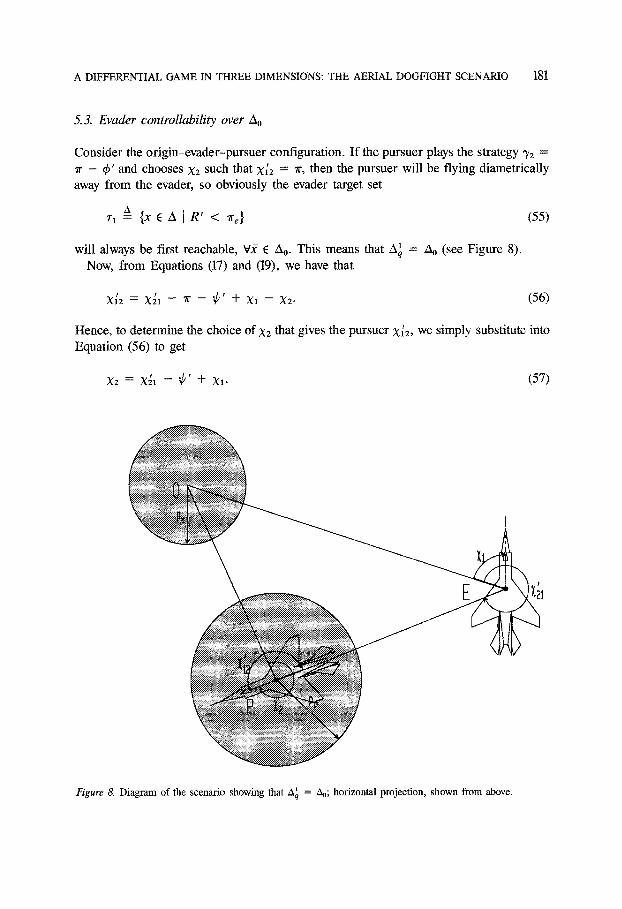
Consider the origin-evader-pursuer configuration. If the pursuer plays the strategy 3'2 = 7r - ~b' and chooses Xz such that x~z = 7r, then the pursuer will be flying diametrically away from the evader, so obviously the evader target set

Lx R ' 7" 1 = {X E A ] < 7re} (55)

will always be first reachable, q£ E Ao. This means that ,x~ = ~o (see Figure 8). Now, from Equations (17) and (19), we have that

X;2 = X21 -- 71" -- ~ ' • X1 -- X2. (56)

Hence, to determine the choice of Xz that gives the pursuer X~'2, we simply substitute into Equation (56) to get

X2 = X~ - ~" + X~. (57)

Figure & Diagram of the scenario showing that/~ = ~o; horizontal projection, shown from above.


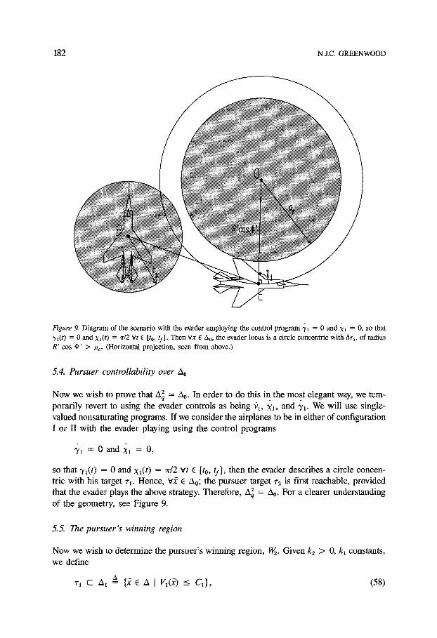
Figure 9. Diagram of the scenario with the evader employing the control program "Y1 = 0 and Xl = 0, so that "r~(t) = 0 and Xl(t) = ~r/2 ¥t E [to, 9]" Then vx E ~o, the evader locus is a circle concentric with 0~, of radius R' cos 4 ' > Pc- (Horizontal projection, seen from above.)

5.4. Pursuer controllability over Ao

Now we wish to prove that ~ = ~o. In order to do this in the most elegant way, we tem- porari ly revert to using the evader controls as being ~ , X1, and "Y1. We will use single- valued nonsaturating programs. I f we consider the airplanes to be in either of configuration I or II with the evader playing using the control programs

~)/1 = 0 and Xl = 0,

so that qq(t) = 0 and xl(t) = 7r/2 v t E [to, tf], then the evader describes a circle concentric with his target r~. Hence, VY E 4o; the pursuer target r2 is first reachable, provided that the evader plays the above strategy. Therefore, 4 8 = ~o. For a clearer understanding of the geometry, see Figure 9.

5.5. The pursuer's winning region

Now we wish to determine the pursuer 's winning region, W2. Given k2 > 0, k~ constants, we define

~-, c 4 , ~ {~ ~ 4 I v,(x-) ___ c ,} , (58)


and

~ ~ ~x~ ~ {2 e ~ I v : (b _< c~}, (59)

where

A r2 = {£fi A I r ' < Pp}, (60)

t a k i n g C 1 ~-- De, C2 -- pp - £, and rl defined as per Equation (55), where e > 0 is arbitrarily small. The purpose of this e is to ensure that we have penetration of the firing region by the airplane so that it is within range of the opponent's missile system, rather than simply touching the periphery of missile range. This is the reason we have concentrated on rendezvous and capture, rather than on collison.

From the Getz-Leitmann theorem, given

~ 2 kl Wz(V~, I"2, k,, kz) ~ ~ A \ (T 1 U AI) I V I ( ~ -- C1 k2 ) . (61) < V2(x-) - c2

and that 3 quadruple {VI('), V2('), kl, k2}, a strategy/52(.) ( p2 and a function/),2(') " A ~ v nonempty subsets of U 2 such that

(i) /5,~(£(t)) =/5,2(x -) v(£, t) 6 a x R',

-2 (ii) ¥2 E W2(VI, Vz, kl , k2) and vt7 z E p,(x-),

;sEu~, ' VV2(x-)" f (£ , Ft', t7 2) _< -k2 < 0

inf VV~(x-).f(£, ~t ~, t~ 2) > - k~ (62) fi~EU 1

and conditions of admissible strategies and no finite escape time apply, then Wz(V~, V2, kl, k2) is 2-winning.

Here we use configuration II (origin-pursuer-evader), and take the Liapunov functions to be Vl(x-) ~ R'(t) , Vz(x-) ~= r'(t).

Now from Equation (42),

?'(t) = - v l cos X21 cos(~{1 "~ ¢ ' ) ~- v2 cos X;2 cos('y2 -~- (])')

= -v~ cos(xh - 7r - ¢ ' + x2 - Xl) cos (3q + ¢ 9 + v2 cos x;2 cos(~/2 + ¢ ' ) (63)

(from Equation (32)).


Note that we regard if ' here as not being directly controllable by player 1. Let us consider Equation (62), which says

sup ?'(t) < -k2 < 0, assuming 3k2 > 0. ")'l,X1

Using Equation (63), we find that

sup ?( t ) = sup - v , c o s ( x ; 2 - r - i f ' + X2 - X , ) cos (71 + ¢ ' ) ~/1,X1 7,,X1

+ V 2 COS X;2 COS('y2 + q~')

= V 1 "t- V 2 COS Xlr2 COS('~2 "t- ~ t ) ,

where either X, = X~2 + X2 - 7r - if' and 3"1 = -qS' + 7r, or else X, = x~2 + Xz - ~ '

and 3'a = - 4 K Therefore,

V 1 + V 2 COS X;2 COS(3'2 - ~ ' ) -< - k 2 < 0 ,

v2 + cos X12 - -< -k2 < 0. (64)

I f this is to hold for all X~z, 3'2, q~' and for some k2 > 0, we must have

v ~ < 1. V2

In other words, we need pursuer speed greater than evader speed. Hence, the maximum possible value for k2 is (from Equation (64))

k2 = v2 - vl. (65)

Consider, furthermore, Equation (62), which says

inf R ' ( t ) >. - k l . "YI,X,

Using Equation (41), we find

inf /}'(t) = inf - v 2 cos X2 cos(3"2 + 4~') >_ - k , ; qq,X1 3q,Xl

hence,

v2 cos X2 cos(3'2 + ~ ' ) < k,. (66)

A D I F F E R E N T I A L G A M E IN T H R E E DIMENSIONS: T H E A E R I A L D O G F I G H T S C E N A R I O 185

Since kl must be greater than the left-hand side of Equation (66) for all X2, 3'2 and ~b ', then the minimum upper bound must be kl = v2. From Equation (64), we deduce a form for k2 to be

k2 = 1 + 6 for some 6 ~ [0, co). (67)

Also, we have from Equation (64) that

cos x1'2 cos(3"2 + ¢ ' ) < - - V 1 V 1

= - c o s X1'2 cos(3'2 + ~ ' ) > - - . ]?2 V2

Then

kl 1 + 6 1 + 6 - - - ~ V l ( x - ) - C l >

k2 1 vi 1 vl V 2 12 2

(68)

- - [V2(x~ - C2]. (69)

The winning region can now be maximized by selecting the case 6 = 0. This is equivalent

from Equation (31).

to either one of two strategy pairs, namely,

(i) 9(1'2 = 0 and 3'2 = 7r - if '

or else

(ii) X;2 = 7r and 3'2 = -q~'.

But X~'2 = 7r + X~I + ~ ' + Xl - X2, from Equation (34). Hence, Case (i) is equivalent to saying that

3"2 = ~r - 4~' and )~2 = 7r + Xdl + ~b' + x~, (70)

or, refining this a step further by expressing ~b' in terms of the evader's parameters,

3'2 = -~b' + 7r and

[ r ' e o s O' 1 X2 = 7r + X~t + X~ + arcsin R ' c o s ¢ ' ' s i n ( x l + X~) (71)


Similarly, Case (ii) is equivalent to saying

3'2 = - ~ b ' a n d X2 = X21 "~ ¢ ' "~- Xl , (72)

or, expressing this another way

, I r ' cos ~b' ] 3"2 = -~b' and X2 = Xl + X2~ + arcsin R ' c o s ~ ' ' s i n ( x l + X~a) • (73)

We now have a multiplicity of strategies of two. Both give 6 = 0, but here the former case of 3'2 = 7r - 4~' and X2 = 7r + X~l + ¢ ' + Xl is the physically optimal solution, giving that the winning strategy of the pursuer is to head towards the evader with zero horizontal relative heading angle, and along the vertical line-of-sight. Using this strategy, Equation (60) implies

R'(t) - P e > - -

1 VI V2

[r'(t) - & + el

for arbitrarily small e > 0. Hence, the maximum winning region for the pursuer in configuration II is given by

w~(y , , v2, k , , k 9 =

( x E (A, r2) t R'(t) Pe > [r'(t) pp]~. V 2 A \ U

1~ 2 - - y 1 J (74)

5.6. The evader's winning region

Now in order to determine the evader's winning region, consider the airplanes in configuration I (origin-evader-pursuer). Given kl > 0, k2 constants, we define

~-, D z~, ~ {5 ~ z~ I Vl(X-) --- C,}, (75)

7"2 C A2 ~ {~ ¢ A [ V2(x-) < C2}, (76)

where C1 = pp - e for arbitrarily small e > O, C2 = Pe, V~(x-) ~ R'(t) and V2(x-) ~ r'(t):

(~? k, k2 ) w , ( v , , v2, k , , k2) = ~ a \ (~-1 U ~,2) I V,(x~ - - C1 > V~(x~ - C2 "


We apply here the first statement of the Ge tz -Le i tmann theorem given in this article, namel) ;

that in te rms of the 1-winning region. F r o m Equat ions (52),

s u p / ~ ' ( t ) -< - k l < 0. ~2,X2

Using Equat ion (26), we have

s u p / ~ ' ( t ) = sup - v l cos X~ cos(71 + ~ ' ) "Y2,X2 3"2,Xz

= - v l cos X1 cos(3"t + ~ ' )

--< - k l < O.

We deduce then that

121 ~-~ V 1 COS X1 COS(3'I "~- (~ ' ) ~-~ kl > 0 , VX1, 3"1, cI) t

which means that the constant k I c a n take the form

vl for some ~ E [0, oo). k l - l + 6

F r o m Equat ion (28),

~:'(t) = - v 2 cos X~2 c0s(3'2 + 4~') + vl cos X~I cos(3'1 + 4 ' ) ,

and Equat ion (21) = X~2 = X~l - 7r - i f ' - X2 + Xl. Therefore,

• t: '(t) = - v 2 cos[x~l -- 7r - ~ ' - X2 + Xl] • cos(3'2 + ~b')

+ vl cos x ~ cos(3"~ + ~ ' ) ,

Equat ions (52) = inf t: '(t) _> - k z , "/2,X2

R ' cos ~ ' inf ~:'(t) = inf -v2 c o s ¢ ' r ' cos ~b' X2" cos(3'2 + q~')

')I2,X2 ~2,X2

(77)

(78)

(79)

(80)

+ vl cos (x~0 c0s(3"1 + ¢ ' )

= - v 2 + vl cos x~l cos(3"~ + q~') for e i ther

X2 = X~l - ~b' + Xl and 3'1 = -4~ ' + 7r

X2 X~l 7r - ¢ ' + X1 and 3'2 = - ~ b '

188 N J . C . G R E E N W O O D

~_~ - - V 2 - - V 1

>_ - k 2.

Therefore,

- - V 2 -~ V 1 COS X21 COS( '~l -~- (~ ' ) ~-~ - - v 2 - - v1 ~-~ -k2 ,

which is equivalent to saying that

k2 >- v~ + vz > - v ~ cos X~l cos(7~ + ¢ ' ) + v2. (81)

Since the left-hand side of Equation (81) must be greater than or equal to the right-hand side for all values of X~, Yl and 4~ ', we have that the least such value for k2 is k2 = Vl + v2.

Now, using Equation (65), the Getz-Lei tmann theorem implies that

V1

1 + 6 vl + v2 R'-Oe-- > r ' -- Op + e for arbitrarily small e > 0.

Therefore,

r ' - pp + e > - -

For 6 = 0, this gives

vl + v2 (1 + tS) • ( R ' - Pe). V1

r ' - Pe + e > vl + (R' - 0 e ) , (82) V1

where 5 = 0 is synonymous with either of the two strategies

3'1 = 7r - i f ' and XI = 7r

o r

~ = - ~ ' and xl = 0.

Again we have a multiplicity of strategies, and here it is the latter case that is physically optimal, giving the evader the strategy of heading towards the origin with vertical flight- path angle Yl = - ~ ' , and horizontal heading-path angle X~ = 0.

Thus the maximum winning region for the evader in configuration I, given by using the above strategy, is

A D I F F E R E N T I A L G A M E IN T H R E E DIMENSIONS: T H E A E R I A L D O G F I G H T S C E N A R I O 189

WI(V~, V2, k~, kz) = ~Y E A \ (71 U Az) I r ' ( t ) - Op > - - 7 Vl + V2

(R'(t) - P e ) ~'- V1 J

(83)

We note here that successful use of the Getz-Leitmann theorem to determine W,. and the corresponding winning strategy is strongly dependent upon the initial correct choice of configuration geometry. If an attempt is made to ascertain W2 in configuration I or vice versa, then the Getz-Leitmann theorem appears to be of little use.

5.7. M u t u a l kil l

We now turn our attention to strategy pairs (/51, /~2) E P1 X p2 which culminate in the mutual destruction of both players--the option of mutua l kil l . This is an option among strategies that appears to have been sadly neglected in the literature. First of all, we note that if we strictly enforce the axiom of game termination at the event of either player being destroyed, then in this case we must restrict ourselves to such pairs (fit,/3~) as ensure simultaneous destruction. This is because the game would terminate immediately after the destruction of the first aircraft. If simultaneous destruction does not take place, this then leaves the other aircraft as the survivor, and the game finishes here.

However, consider the case where both aircraft are doomed to nonsimultaneous (i.e., consecutive) destruction, due to the control programs of each other's respective opponent. Such a situation cannot be considered in the context of the previous axiom of game termination, and does not appear to have been ever addressed in the literature. If, however, we relax this axiom of termination so that given the time of the event of player i's destruction,

i t~ > to 3~ > 0 such that

i l t s - gl l < ~,

where t f i s the time of termination of the game, then we can consider "posthumous" strategy pairs ~ , / 5 ~ ) E p t × p2 such that given e > O,

• i " 36 > 0 such that l[tf - t~.ll < ~ ~ tlt~ - t~ll < a < ~; t,, t~ > to for i • j .

If we considered the game-history of some trajectory for this situation, it would appear as shown in Figure 10.

Such posthumous strategies would typically involve the dynamic flight envelopes of the aircraft. For example, given a scenario where the pursuer is guaranteed first-reachability of the evader before the evader can reach his origin-centered hemisphere of safety, the evader would try to maximize the time interval before interception. A posthumous mutual-kill strategy pair would be for the pursuer to intercept the evader regardless, while the evader ensures that after interception the pursuer has inadequate time to maneuver to avoid the hemisphere of safety.

N.J.C. GREENWOOD

Figure 10. Graph of the game history of some trajectory displaying consecutive destruction. The strategy pairs resulting in consecutive destruction are referred to as "posthumous" pairs.

Definition 3. Given an admissible program& E pi and some trajectory &pi, ., iO, to, .) such that

we define the posthumous strategy € Pj to be a control program such that

and that it;, ti < tf so that for all &2{, t!, .) E Xi, which are selections to the contingent equation we have that

and secondly, that ;(a, a, 24 ti, t) f l T[ # 0 for vt E [to, tf)

A proper treatment of such posthumous strategies inextricably involves the dynamics of flight. Since this article is predominantly kinematic, we will restrict ourselves to simultaneous destruction (see Figure 11).


Figure 11. Diagrams of two possible simultaneous mutual-kill geometries (configuration I and II, respectively).

We can visualize these geometries by considering a cross section of state space involving R' and r'. In terms of configuration ]I, such a diagram would be as shown in Figure 12.

Similar diagrams appear in [2] and [18], where they are used to discuss ordinary target sets, and are then modified to discuss/~-combat games.

Due to the phenomenon of instantaneous destruction, although

A {:~e ~ I x e ~1 n ~-2}

is a zone of mutual destruction, only

~ {~ ~ ~ I ~ ~ a~-~ n a~-2} c z

0 Figure 12. Diagram of state space.

Region of pursuer destruction

Simultaneous mutual kill . - ' " Re~ion of evader

. - ' " .-'-destruction

Pe ~


provides "usable" termination points for the game, in the sense of Isaacs [21]. W~2 can then be determined using the Retrogression Principle of [21], retro-integrating from ~.

5.8. Map summary

In summary, the map of the game (as per Figure 7) is as follows: Defining Ao as per Equa- tion (54), we have

A ~ = Ao,

A~ = Ao,

4 n = 0 ,

W 1 = I x E z~ \ (T 1 U m2) t r '(t) -- pp > VI V1 "~ "V~2 [R'(t) - Pelt in configuration I,

W2 = ~Y E 4 \ (41 U r:) I R'(t) - Pe > v2 [r'(t) - pp]~- in configuration II,

L V 2 -- V 1 J W12 ~ 0,

RNGO = ao \ (W~ U W,2 U Wg.

We now turn our attention to various surfaces of interest within 4o.

6. O n permeabil i ty of surfaces, and barriers

61. Nonpermeability

In this section we will consider the existence and nature of such entities as nonpermeable surfaces, semibarriers, and barriers, and then apply these concepts to this air combat scenario. We refer the reader to Skowronski and Stonier [22].

We consider the map of the game in the situation where W i ;e 0 and W~ f3 W2 = 0; i E {1, 2}. We will define the semineutral zone f o r player i At,, or the i-neutral zone, by the following statement:

• = i (84) zX~v a A \ a e.

This is the region from which player i cannot win strongly. We will define the neutral zone as being the intersection of the i-neutral zones, that is,

A N ~ A~ n a~ .


exter~ 1

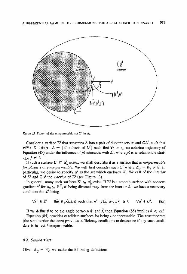
Figure 13. Sketch of the nonpermeable set Ei in A o.

Consider a surface ~i that separates A into a pair of disjoint sets A i and CA/, such that ¥~o ~ ~i 3/~j(.) : A ~ {all subsets of U j } such that Yt > to, no solution trajectory of Equation (48) under the influence of ~ intersects with A i, where ~ is an admissible strategy, j ~ i.

I f such a surface ~ i ~ A~ exists, we shall describe it as a surface that is nonpermeable for player i or i-nonpermeable. We will first consider such z i where A~ = W/ ~ 0. In particular, we desire to specify A i as the set which encloses W/. We call A i the interior of ~i and ~ Ai the exterior of r~ i (see Figure 13).

In general, many such surfaces E i c A~ exist. I f ~i is a smooth surface with nonzero gradient ~i for Ao c ~N, tii being directed away from the interior A i, we have a necessary condition for ~i being

v~ ° e E g ~ e/5~(~(t)) such that h i • j?(~, t~ 1, ~2) >_ 0 Vu i ~ U i. (85)

I f we define 0 to be the angle between ~i and f, then Equation (85) implies 0 < 7r/2. Equation (85) provides candidate surfaces for being i-nonpermeable. The next theorem

(the semibarrier theorem) provides sufficiency conditions to determine if any such candidate is in fact i-nonpermeable.

62. Semibarriers

i = Wi ' we make the following definition: Given AQ


Definition 4. The boundary of W i, aW i, shall be called a semibarrier B i for player i if it is j-nonpermeable, j ~ i.

Theorem 2 (semibarrier theorem). A set zi partitioning A into two disjoint sets A i and GA i with W/ C A i is nonpermeable for player i if given ~i c 0 (open) c_ A, there is a 61 function I1/ : fl x ~1 and a strategy fi~ E PJ such that v(#, t) E (A i [7 fl) x ~1, we have

(i) Vi(Y, t) < Vi(z., t) VY. E S, i, t E ~' .

(ii) For each fiJ E/3J(Y, t),

av~ _ Ot + VVi(Y' t) " f (Y , t, u ~, fi~) _> 0 VtT' E U i, t >_ to; i ~ j. (86)

We note here that if ~i is defined by a V/-level,

VVi(.~, t) ~ t hi

then case (ii) becomes also a necessary condition and defines the j-nonpermeable surface. i \ AJQ, j ~ i. As an immediate Now consider the case where A~ (7 A~ ~ 0; W/ = AQ

corollary of Theorem 2, we have the following:

Corollary 1. The boundary

~ ~ 0A~ \ int Z~Ja

is a semibarrier B i for player i if given E / c fli (open) c A and if 3C ~ function V/ : ~'~i X ~1 ~ ~1 and a strategy/~J E PJ such that

V(Y, t) E [(int W/) O f]i] × ~ ,

conditions (i) and (ii) of Theorem 2 apply (see Figure 14).

6 3. The semibarrier for the pursuer

Now consider the semibarriers for the pursuer. Defining

E, ~ ~ OA~ \ int A~,

we will check using the above sufficiency conditions that ~.~ is a semibarrier for the pursuer.


Figure 14. Diagram showing E~.

Vt Jr V2 ( R t -- De) and A0] r ' - Op -- Vl

( R ' - Oe) >- v------L~z ( r ' - pp) ~.. (87) V2 -- Vl J

The sets W1 and W2 are open. Note here that mutual kill is possible; in other words,

~x b n % = w , 2 # o .

However, W/ ~= Ab \ ~ implies that W~ n w2 = 0, so these sets are disjoint, due to the opposing objectives of the players.

Take CzX 2 = W~ so that ~ C zX 2. Consider the Liapunov function

V2 . ~ 4 ~ ~1

defined by

(v~ + v2] . _ V 2 ( R ' , r ' , v l , v2) = 1 + r ' - pp - v l (17' Pe). J

(88)


Now

and

V z = 1, vYE El,

Vz < 1, YY E A 2,

and 0 VJOt = O. We will use the geometry of configuration I (or igin-evader-pursuer) here. For this Liapunov function

I --V 1 COS X1 cos(~l "q- iI~') 7 M = - v 2 cos X~z cos(~{2 + q~') + Vz cos X21 cos('y1 + qS')

1)1 i'z

In the context of this discussion, we are interested only in the regions for which vl = 0 and ~)2 = 0. Therefore,

VV2 " f = (vl + v2) cos XI cos(3q + ~ ' ) - v2 cos X;2 cos('y2 + ¢ ' )

+ vl cos X~l cos(7~ + q~').

I f the strategy/5 ~ for the evader is 71 = - ¢ ' and Xl = 0, then

VV2 " f = vl[1 + cos(x;2 + ~b' + X2 - nO cos (~b' - ~ ' ) ]

+ v2[1 - cos X~'2 cos(72 + 4~')]

-> 0 V')'2, X2-

Thus, the conditions for the theorem on semibarriers are satisfied, so E. ~ is a semibarrier for the pursuer.

6.4. The semibarrier for the evader

Now consider semibarriers for the evader. Defining

E, z ~ OA~ \ int A~,

we will check that E 2 is a semibarrier for the evader.

VV2.f= I (vl vl+ v2), l 'V~(R ' -Pe) ' l (R ' -pe) l " ~ ' I ' v l vl

where


Let

(r' - pp) E2 = E A 0 [ R ' - Pe - v2 Vz_ v1 and

VI + V2 (r' - pp) > (R' - p e ) ~ ~.

Vl J (89)

m

Here we will use configuration II (or igin-pursuer-evader) , with A1 = W2 and W~ C A1. Consider the Liapunov function V~ : ~4 _~ ~1 defined as

VI(R', r', vl, v2) ~ 1 + R' - Pe V2

V 2 -- V 1 (r' - Op). (90)

Clearly,

V I = l ¥ 2 ~ E 2,

and

V1 < 1 v2 e A',

and OVJOt = 0. For this Liapunov function

I --V2 OVl OVI 1 V V I ' f = 1, v2 - v1 " Ovl' Ov2

- v z cos X2 c0s(3,2 + ~ ' ) - v 1 cos X21 cos(~l + (~') "1- 122 cos X;2 cos(~2 "~- (~')

v2

Here we are interested only in the regions for which vl = 0 and v2 = 0. In such regions,

VV1 " f = - v 2 cos XE cos(y2 + qS') V 2 -- V1 - - COS Xlt2 COS('y2 + (~t)

-[" V1 V2 COS X21 COS("YI q- ¢ ~'). V 2 -- V1

Suppose the pursuer plays the strategy cos Xl'2 cos(Tz + ~ ' ) = -1 , i.e., he plays either

(i) 3'1 = r - 4~' and X;2 = 0


o r

(ii) 72 = -~b' and X~'2 = 7r.

Consider the case where the pursuer opts for Option (i). Then from Equation (33),

X~2 = r = X2 = X~, + ¢ ' + X~ + 7r,

VV, • f = -v2 COS[X21 "F @t .~_ Xl -F r l cos(¢' - ~ ' + T r ) + - - v 2 -- v 1

"F F1 112 COS X21 COS('~I -1- ~ ' ) v 2 - - v i

V 2 Icos[x~, + ¢ ' Xl] cos (¢ ' ¢ ' ) + / q

V2 + 1/2 -- V 1 V 2 -- V 1 /

--- v2[cos[x~l + ¢ ' + xl] cos(,I,' - ¢ ' ) + 1]

>__0.

Theretbre, .'. ~ • f > 0, and hence Z~ is a semibarrier for the evader.

65. The barrier

Given that the semibarriers B 1 and B 2 exist, we define the barrier to be

B ~ B 1 0 B 2,

provided this intersection is nonvoid. We define semipermeability of a surface E as follows:

Definition 5. Given i-nonpermeable sets ~ ' and E 2 we describe

~ = ~ 1 0 E 2

as a semipermeable surface, provided it is nonempty.

This means that ¥20 ( ~,

t ' -3t3' such that 3£(/3', 2 °, t) N interior ~2 = 0, Yt _ to

~, 3/3 z such that 3£(/52, 2% t) N interior E 1 = 0, v t _> to.


On this surface ~, there exists a strategy for player 1 to prevent penetration into the interior of ~z, and similarly there exists a strategy for player 2 to prevent penetration into ~1.

From this definition, clearly B is a semipermeable surface, and it locally partitions A into the winning regions W~ and WE. The semibarriers are defined so that each i-semibarrier is unique for player i. Thus, the barrier surface is unique, if it exists.

In the case of the 3-D aerial dogfight, W~2 N 9. From Figure 14 we can see that

W12 ~ 0 = ~ , ~= ~ , N ~2 = B 1 0 B z = B ~ 0,

and therefore the barrier exists.

7. Conclusion

In this article, an aerial dogfight in three dimensions between identical aircraft was studied, by means of superimposing two semigames. Each airplane possessed combined qualitative objectives of capture or rendezvous with a target while avoiding an antitarget for all time prior to target capture. Although the roles of "pursuer" and "evader" were regarded as predetermined and fixed throughout the duration of each two-target semigame, these semigames were interfaced by being simultaneously superimposed throughout the entire duration of play, which in turn produced the game.

A three-dimensional spherical polar coordinate system was created to describe the geometry of the game in two basic configurations, with the equations of motion calculated for each. Dynamic equations of flight using point-mass aircraft were adopted to establish a kinematic model.

Controllability and winning regins were calculated for each player, the latter using a Liapunov-function approach via the Getz-Leitmann theorem. This was done by introducing a technique of dissecting game trajectories into segments defined by the values of their control variables. The existence of multiple candidates for winning strategies generated by this theorem for a given winning region were noted. In each case, only a single candidate appeared actually to be a winning strategy. Subsurfaces of the boundaries 0W/of these winning regions were proved to be semibarriers for the game using sufficiency conditions, and the barrier for the game was proved to be nonvoid. The mutual kill region was shown to be nonvoid, and the concept of posthumous strategies was introduced.

References

1. M.D. Ardema, M. Heymann, and N. Rajan, "Combat games" JOTA, ~1.46, no. 4, pp. 391-398, 1985. 2, M. Heymann, M.D. Ardema, and N. Rajan, "A formulation and analysis of combat games" NASA TP2487,

vol. 54, no. 1, June 1985. 3. A.E. Bryson, M.N. Desai, and W.C. Hoffman, "Eneregy-state approximation in performance optimization

of supersonic aircraft,' J. aircraft, vol. 6, no. 6, pp. 481-488, 1969. 4. W.Y. Peng, and T.L. Vincent, "Some aspects of aerial combat" A/AA J., vol. 13, no. 1, pp. 7-11, 1975.


5. C. Hillberg, and B. Jfirmark, "Pursuit-evasion between two realistic aircraft," J. Guidance, vol. 7, no. 6, pp. 690-694, 1984.

6. H.J. Kelley, and L. Lefton, "Supersonic aircraft energy turns," Automatica, vol. 8, pp. 575-580, 1972. 7. H.J. Kelley, and L. Lefton, "Differential turns," AIAA J., vol. 11, no. 6, pp. 858-861, 1973. 8. H.J. Kelley, 'N threat-reciprocity concept for pursuit-evasion," IFAC Differential Games Conference, June

7-10, 1976. 9. A.W. Mertz, "To pursue or to evade--that is the question;' J. Guidance, vol. 8, no. 2, pp. 161-166, 1985.

10. N. Rajan, and M.D. Ardema, "Interception in three dimensions: an energy formulation, J. Guidance, vol. 8, no. 1, pp. 23-30, 1985.

I 1. J.V. Breakwell, "Pursuit of a faster evader;' Int. Conf. Differential Games, Warwick, 1974, pp. 243-256. 12. J.M. Skowronski, "Winning controllers for nonlinear air combat game with reduced dynamics;' Proc, AIAA

Guidance, Navigation and Control Conference, Minneapolis, 1988, pp. 866-873. 13. M. Falco, and HJ. Kelley, "Aircraft symmetric flight optimization;' Control Dymnamic Syst., vol. t0, pp.

89-129, 1973. 14. L Shinar, A. Merari, D. Blank, and E.M. Medinah, "Analysis of aerial turning maneuvers in the vertical

plane;' J. Guidance Control, vol. 3, no. 1, pp. 69-77, 1980. 15. J.M. Skowronski, and RJ. Stonier, "The barrier in a pursuit-evasion game with two targets," Comput. Math.

Applic., vol. 13, no. 1-3, pp. 37-45, 1987. 16. W.M. Getz, and G. Leitmann, "Qualitative differential games with two targets," J. Math. Anal. Applic.,

vol. 68, pp. 421-430, 1979. 17. J.M. SkowrorLski, and R.J. Stonier, '~A map of a two person qualitative dift~rential game;' Proc. AIAA Guidance,

Navigation and Control Conference, Monterey, 1987, pp. 56-64. 18. M.D. Ardema, M. Heymann, and N. Rajah, 'Nnalysis of a combat problem: the turret game," JOTA, vol.

54, no. 1, pp. 23-42, 1987. 19. C.R. Hargraves, and S.W. Paris, "Direct trajectory optimization using non-linear programming and colloca-

tion," J. Guidance, vol. 10, no. 4, pp. 338-342, 1987. 20. H. Ikawa, "A unified three-dimensional trajectory simulation methodology," J. Guidance, vol. 9, no. 6, pp.

6504556, 1986. 21. R. lsaacs, Differential Games. Wiley: New York, 1965. 22. J.M. Skowronski, and RJ. Stonier, "Two-person qualitative differential games with two objectives;' Comput.

Math. Applic., vol. 18, no. 1-3, pp. 133-150, 1989. 23. B. Etkin, Dynamics of Flight-Stability and Control, Wiley: New York, 1982. 24. P.K.A. Menon, "Short range nonlinear feedback strategies for aircraft pursuit-evasion,' J. Guidance, Control,

Dynamics, vol. 12, no. 1, pp. 27-32, 1989. 25. A. Davidovits, and L Shinar, "Eccentric two-target model for qualitative air combat game analysis;' J. Guid-

ance, vol. 8, no. 3, pp. 325-331, 1985. 26. P.K.A. Menon, and E.L. Duke, "Time-optimal aircraft pursuit-evasion with a weapon-envelope constraint,"

Proc. the 1990 American Control Conference, San Diego, May 1990, pp. 2337-2342.

Documents

A differential game in three dimensions: The aerial dogfight scenario