A Diagnostic System for Air Brakes in Commercial Vehicles (PDF

A DIAGNOSTIC SYSTEM FOR AIR BRAKES IN COMMERCIAL VEHICLES

A Dissertation

by

SHANKAR RAM COIMBATORE SUBRAMANIAN

Submitted to the Office of Graduate Studies of Texas A&M University

in partial fulfillment of the requirements for the degree of

DOCTOR OF PHILOSOPHY

May 2006

Major Subject: Mechanical Engineering

A DIAGNOSTIC SYSTEM FOR AIR BRAKES IN COMMERCIAL VEHICLES

A Dissertation

by

SHANKAR RAM COIMBATORE SUBRAMANIAN

Submitted to the Office of Graduate Studies ofTexas A&M University

in partial fulfillment of the requirements for the degree of

DOCTOR OF PHILOSOPHY

Approved by:

Co-Chairs of Committee, K. R. RajagopalD. Swaroop

Committee Members, Jo W. HowzeJohn L. Junkins

Head of Department, Dennis O’Neal

May 2006

Major Subject: Mechanical Engineering

iii

ABSTRACT

A Diagnostic System for Air Brakes in Commercial Vehicles. (May 2006)

Shankar Ram Coimbatore Subramanian, B.E., University of Allahabad;

M.S., Texas A&M University

Co–Chairs of Advisory Committee: Dr. K. R. RajagopalDr. D. Swaroop

This dissertation deals with the development of a model-based diagnostic sys-

tem for air brake systems that are widely used in commercial vehicles, such as trucks,

tractor-trailers, buses, etc. The performance of these brake systems is sensitive to

maintenance and hence they require frequent inspections. Current inspection tech-

niques require an inspector to go underneath a vehicle to check the brake system

for possible faults, such as leaks, worn brake pads, out-of-adjustment of push rods,

etc. Such inspections are time consuming, labor intensive and difficult to perform

on vehicles with a low ground clearance. In this context, the development of an on-

board/handheld diagnostic tool for air brakes would be of significant value. Such a

tool would automate the brake inspection process, thereby reducing the inspection

time and improving the safety of operation of commercial vehicles. In this disser-

tation, diagnostic schemes are developed to automatically detect two important and

prevalent faults that can occur in air brake systems – leaks and out-of-adjustment of

push rods.

These diagnostic schemes are developed based on a nonlinear model for the pneu-

matic subsystem of the air brake system that correlates the pressure transients in the

brake chamber with the supply pressure to the treadle valve and the displacement

iv

of the treadle valve plunger. These diagnostic schemes have been corroborated with

data obtained from the experimental facility at Texas A&M University and the results

are presented.

The response of the pneumatic subsystem of the air brake system is such that it

can be classified as what is known as a “Sequential Hybrid System”. In this disserta-

tion, the term “hybrid systems” is used to denote those systems whose mathematical

representation involves a finite set of governing ordinary differential equations corre-

sponding to a finite set of modes of operation. The problem of estimating the push

rod stroke is posed as a parameter estimation problem and a transition detection

problem involving the hybrid model of the pneumatic subsystem of the air brake sys-

tem. Also, parameter estimation schemes for a class of sequential hybrid systems are

developed. The efficacy of these schemes is illustrated with some examples.

v

To my Parents, Sister and Teachers

vi

ACKNOWLEDGMENTS

I am very fortunate to be a student of Professor K. R. Rajagopal and Professor

D. Swaroop. It is a great privilege to work under the guidance of Professor K.

R. Rajagopal and I convey my sincere thanks to him for providing me with this

opportunity. I thank him for spending his valuable time in guiding and motivating

me through out the course of this dissertation. I express my sincere gratitude to

Professor D. Swaroop for his immense help through out my graduate studies. I thank

him for all his weekend lectures on control system theory and optimization. I thank

both of them for their patience, support and understanding through out the course

of this dissertation. I thank Professor Jo W. Howze and Professor John L. Junkins

for kindly agreeing to be members of my dissertation committee.

I am indebted to my parents for their love and blessings. It is due to their never

ending support and encouragement that I have been able to reach this position in life.

I can never repay them for their sacrifices in bringing me up and allowing me to study

in the United States. I feel blessed to have a loving sister, brother-in-law and nephew,

and I thank them for their love and affection. I thank all my friends for their love

and support. I convey my sincere appreciation to the academic and technical staff in

the Department of Mechanical Engineering at Texas A&M University for their help

and assistance.

vii

TABLE OF CONTENTS

CHAPTER Page

I INTRODUCTION . . . . . . . . . . . . . . . . . . . . . . . . . . 1

A. Background and motivation . . . . . . . . . . . . . . . . . 2

B. Objectives . . . . . . . . . . . . . . . . . . . . . . . . . . . 6

C. Organization of this dissertation . . . . . . . . . . . . . . . 9

II A BRIEF DESCRIPTION OF THE AIR BRAKE SYSTEM . . 11

A. The train air brake system . . . . . . . . . . . . . . . . . . 12

B. The air brake system used in commercial vehicles . . . . . 13

C. Improvements to the basic air brake system and emerg-

ing technologies . . . . . . . . . . . . . . . . . . . . . . . . 19

III THE EXPERIMENTAL SETUP . . . . . . . . . . . . . . . . . . 23

A. Brake system components . . . . . . . . . . . . . . . . . . 23

B. Actuation and motion control components . . . . . . . . . 26

C. Sensing and data acquisition components . . . . . . . . . . 28

IV A MODEL FOR PREDICTING THE PRESSURE TRAN-

SIENTS IN THE AIR BRAKE SYSTEM . . . . . . . . . . . . . 36

A. Existing models for air brake systems . . . . . . . . . . . . 36

B. A model for predicting the pressure transients in the

brake chamber . . . . . . . . . . . . . . . . . . . . . . . . . 38

1. Equations governing the mechanics of operation of

the treadle valve . . . . . . . . . . . . . . . . . . . . . 38

2. Equations governing the flow of air in the pneu-

matic subsystem of the brake system . . . . . . . . . . 42

C. The air brake system as an example of a sequential

hybrid system . . . . . . . . . . . . . . . . . . . . . . . . . 53

D. A brief discussion concerning controlling the pressure

in the air brake system . . . . . . . . . . . . . . . . . . . . 56

V DETECTION OF LEAKS IN THE AIR BRAKE SYSTEM . . . 60

A. A brief review of existing diagnostic tools for air brake

systems . . . . . . . . . . . . . . . . . . . . . . . . . . . . 61

viii

CHAPTER Page

B. A scheme for detecting leaks in air brake systems . . . . . 65

C. Determination of thresholds for the detection of leaks . . . 75

VI ESTIMATION OF THE PUSH ROD STROKE . . . . . . . . . 80

A. Effect of push rod stroke on the pressure transients . . . . 80

B. Schemes for estimating the stroke of the push rod . . . . . 84

1. Scheme 1 – Estimation of the push rod stroke by

discretization of the possible range of values . . . . . . 84

2. Scheme 2 – Detection of the transition from Mode

2 to Mode 3 . . . . . . . . . . . . . . . . . . . . . . . 88

C. Effect of leaks on the estimation of the push rod stroke . . 93

VII PARAMETER ESTIMATION SCHEMES FOR A CLASS

OF SEQUENTIAL HYBRID SYSTEMS . . . . . . . . . . . . . 97

A. The class of systems under study . . . . . . . . . . . . . . 98

B. The proposed parameter estimation scheme when the

transition conditions are known . . . . . . . . . . . . . . . 100

1. Example 1 . . . . . . . . . . . . . . . . . . . . . . . . 106

2. Example 2 . . . . . . . . . . . . . . . . . . . . . . . . 109

3. Example 3 . . . . . . . . . . . . . . . . . . . . . . . . 112

C. The proposed parameter estimation scheme when the

transition conditions are unknown . . . . . . . . . . . . . . 115

1. Example 4 . . . . . . . . . . . . . . . . . . . . . . . . 118

VIII CONCLUSIONS . . . . . . . . . . . . . . . . . . . . . . . . . . . 123

A. Potential impact of this dissertation . . . . . . . . . . . . . 124

B. Scope of future work . . . . . . . . . . . . . . . . . . . . . 124

REFERENCES . . . . . . . . . . . . . . . . . . . . . . . . . . . . . . . . . . . 127

VITA . . . . . . . . . . . . . . . . . . . . . . . . . . . . . . . . . . . . . . . . 140

ix

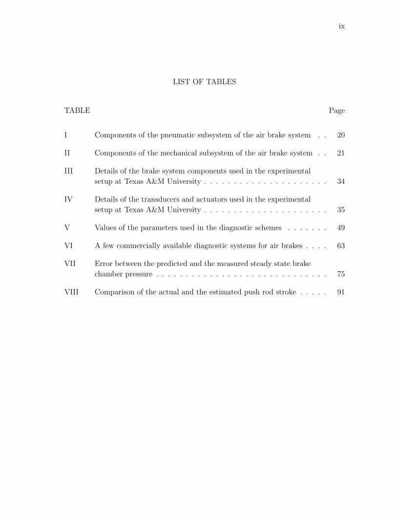
LIST OF TABLES

TABLE Page

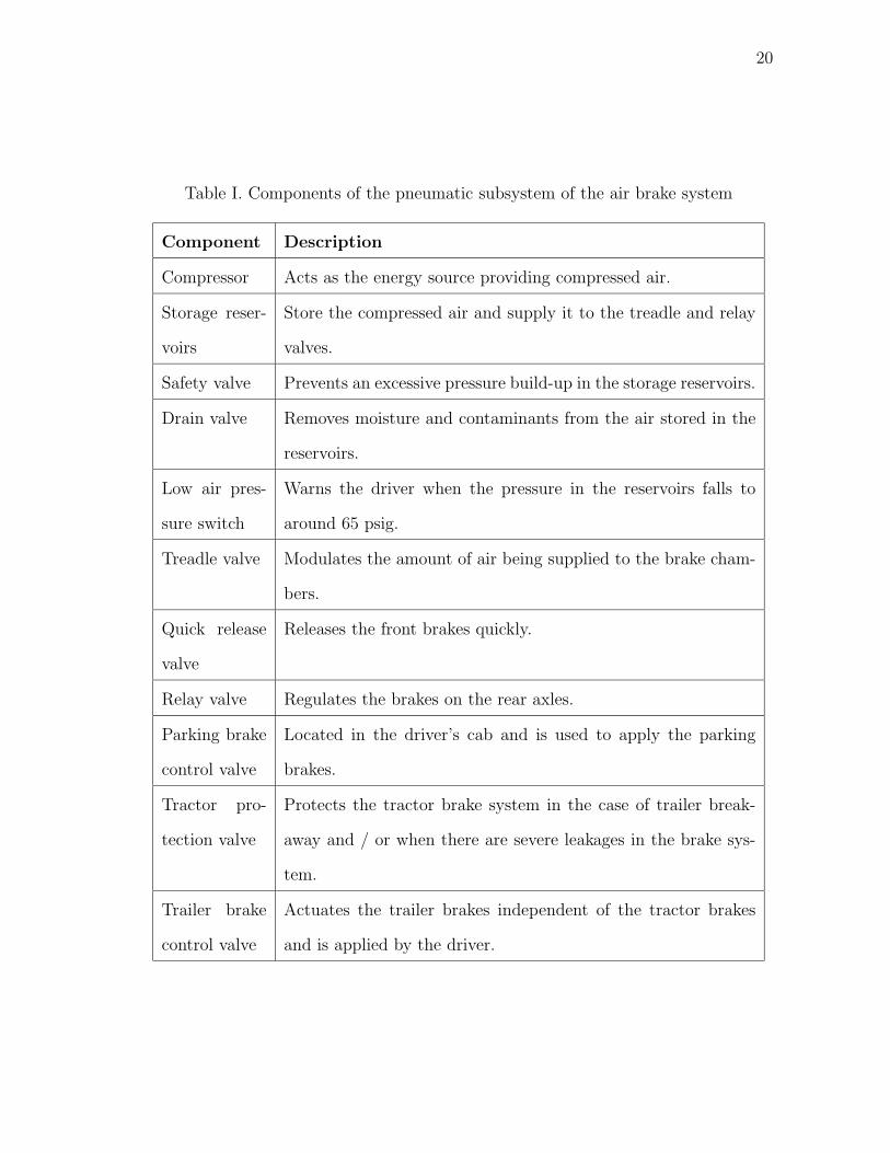
I Components of the pneumatic subsystem of the air brake system . . 20

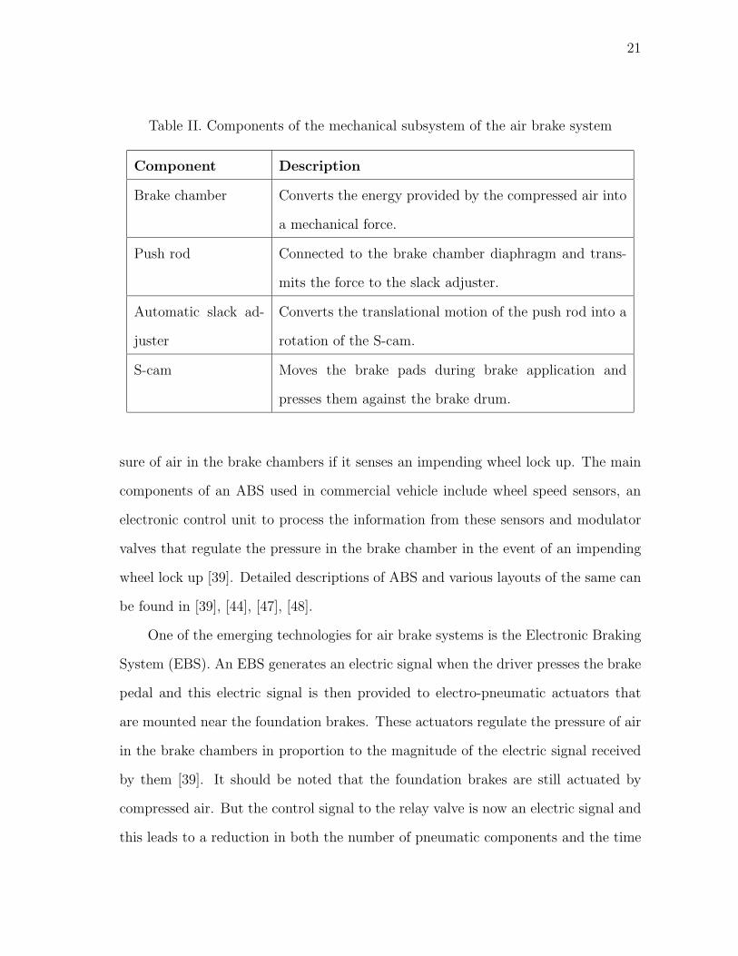
II Components of the mechanical subsystem of the air brake system . . 21

III Details of the brake system components used in the experimental

setup at Texas A&M University . . . . . . . . . . . . . . . . . . . . . 34

IV Details of the transducers and actuators used in the experimental

setup at Texas A&M University . . . . . . . . . . . . . . . . . . . . . 35

V Values of the parameters used in the diagnostic schemes . . . . . . . 49

VI A few commercially available diagnostic systems for air brakes . . . . 63

VII Error between the predicted and the measured steady state brake

chamber pressure . . . . . . . . . . . . . . . . . . . . . . . . . . . . . 75

VIII Comparison of the actual and the estimated push rod stroke . . . . . 91

x

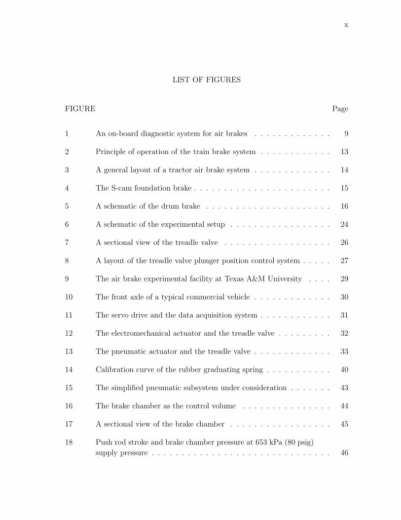
LIST OF FIGURES

FIGURE Page

1 An on-board diagnostic system for air brakes . . . . . . . . . . . . . 9

2 Principle of operation of the train brake system . . . . . . . . . . . . 13

3 A general layout of a tractor air brake system . . . . . . . . . . . . . 14

4 The S-cam foundation brake . . . . . . . . . . . . . . . . . . . . . . . 15

5 A schematic of the drum brake . . . . . . . . . . . . . . . . . . . . . 16

6 A schematic of the experimental setup . . . . . . . . . . . . . . . . . 24

7 A sectional view of the treadle valve . . . . . . . . . . . . . . . . . . 26

8 A layout of the treadle valve plunger position control system . . . . . 27

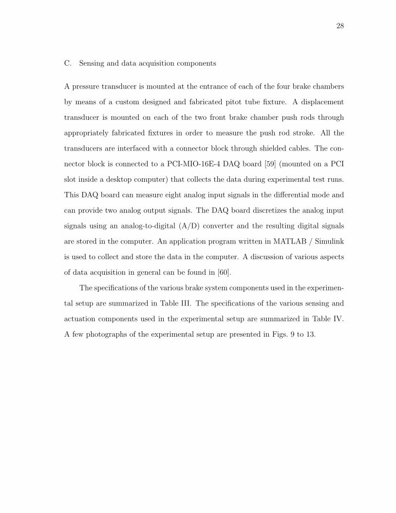
9 The air brake experimental facility at Texas A&M University . . . . 29

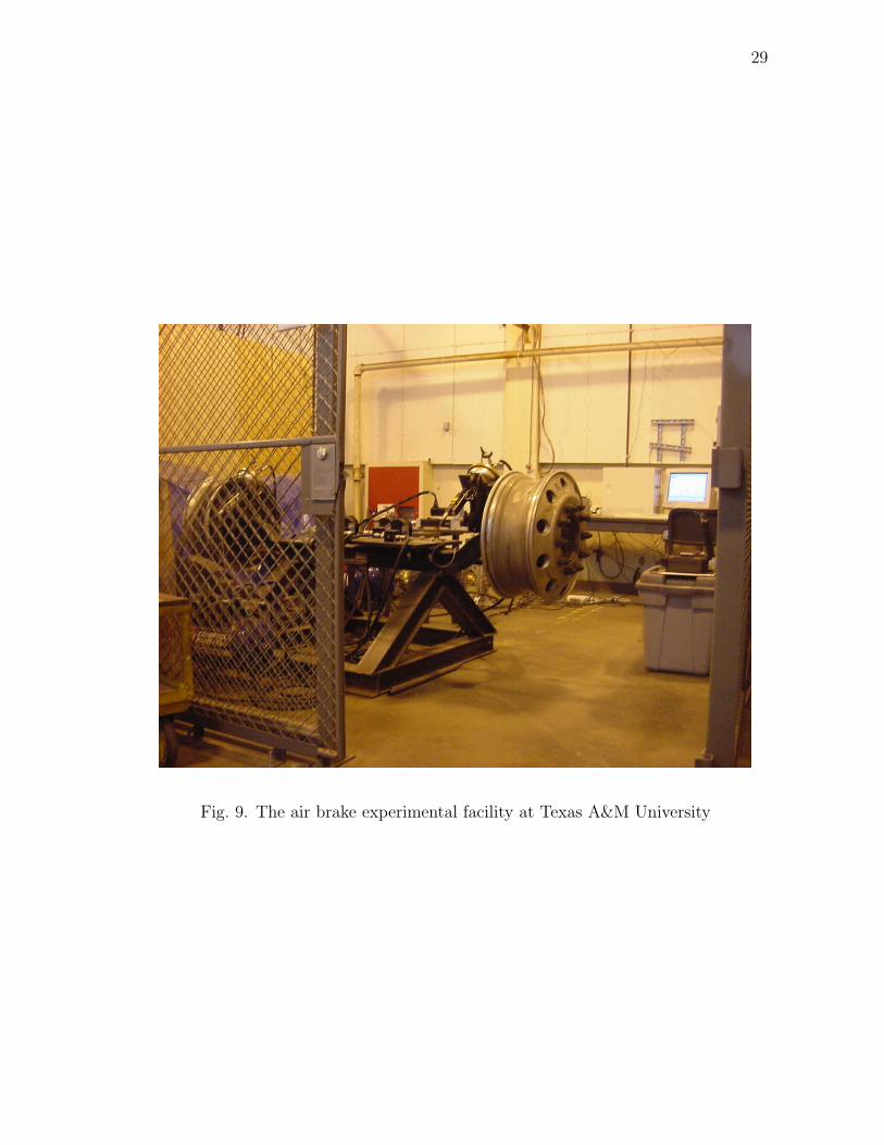
10 The front axle of a typical commercial vehicle . . . . . . . . . . . . . 30

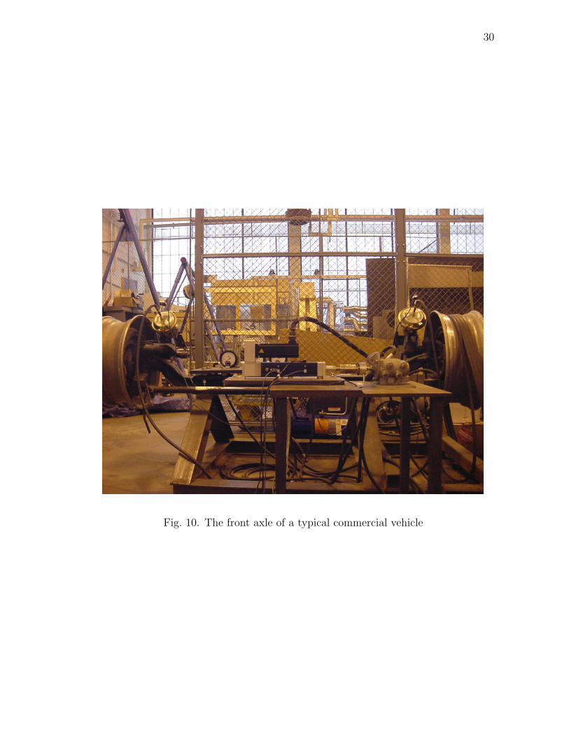
11 The servo drive and the data acquisition system . . . . . . . . . . . . 31

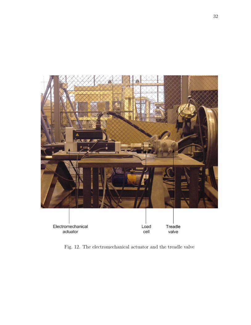
12 The electromechanical actuator and the treadle valve . . . . . . . . . 32

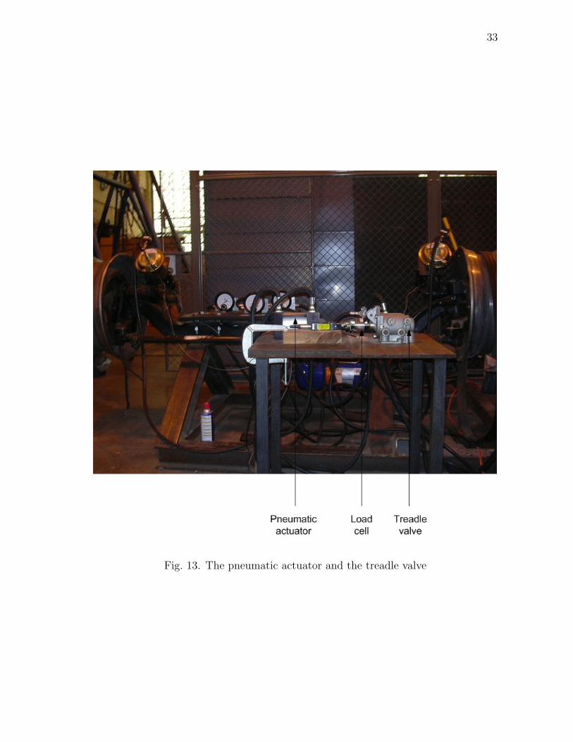
13 The pneumatic actuator and the treadle valve . . . . . . . . . . . . . 33

14 Calibration curve of the rubber graduating spring . . . . . . . . . . . 40

15 The simplified pneumatic subsystem under consideration . . . . . . . 43

16 The brake chamber as the control volume . . . . . . . . . . . . . . . 44

17 A sectional view of the brake chamber . . . . . . . . . . . . . . . . . 45

18 Push rod stroke and brake chamber pressure at 653 kPa (80 psig)

supply pressure . . . . . . . . . . . . . . . . . . . . . . . . . . . . . . 46

xi

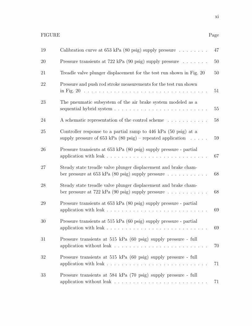
FIGURE Page

19 Calibration curve at 653 kPa (80 psig) supply pressure . . . . . . . . 47

20 Pressure transients at 722 kPa (90 psig) supply pressure . . . . . . . 50

21 Treadle valve plunger displacement for the test run shown in Fig. 20 50

22 Pressure and push rod stroke measurements for the test run shown

in Fig. 20 . . . . . . . . . . . . . . . . . . . . . . . . . . . . . . . . . 51

23 The pneumatic subsystem of the air brake system modeled as a

sequential hybrid system . . . . . . . . . . . . . . . . . . . . . . . . . 55

24 A schematic representation of the control scheme . . . . . . . . . . . 58

25 Controller response to a partial ramp to 446 kPa (50 psig) at a

supply pressure of 653 kPa (80 psig) – repeated application . . . . . 59

26 Pressure transients at 653 kPa (80 psig) supply pressure - partial

application with leak . . . . . . . . . . . . . . . . . . . . . . . . . . . 67

27 Steady state treadle valve plunger displacement and brake cham-

ber pressure at 653 kPa (80 psig) supply pressure . . . . . . . . . . . 68

28 Steady state treadle valve plunger displacement and brake cham-

ber pressure at 722 kPa (90 psig) supply pressure . . . . . . . . . . . 68





31 Pressure transients at 515 kPa (60 psig) supply pressure - full

application without leak . . . . . . . . . . . . . . . . . . . . . . . . . 70





xii

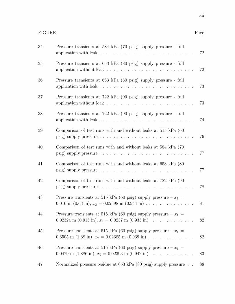
FIGURE Page











39 Comparison of test runs with and without leaks at 515 kPa (60

psig) supply pressure . . . . . . . . . . . . . . . . . . . . . . . . . . . 76







43 Pressure transients at 515 kPa (60 psig) supply pressure – x1 =

0.016 m (0.63 in), x2 = 0.02398 m (0.944 in) . . . . . . . . . . . . . . 81


0.02324 m (0.915 in), x2 = 0.0237 m (0.933 in) . . . . . . . . . . . . 82


0.3505 m (1.38 in), x2 = 0.02385 m (0.939 in) . . . . . . . . . . . . . 82


0.0479 m (1.886 in), x2 = 0.02393 m (0.942 in) . . . . . . . . . . . . 83

47 Normalized pressure residue at 653 kPa (80 psig) supply pressure . . 88

xiii

FIGURE Page

48 Normalized pressure residue at 722 kPa (90 psig) supply pressure . . 89

49 Transition detection at 653 kPa (80 psig) supply pressure . . . . . . . 92

50 Transition detection at 722 kPa (90 psig) supply pressure . . . . . . . 92

51 Comparison of pressure transients with and without leaks at 653

kPa (80 psig) supply pressure . . . . . . . . . . . . . . . . . . . . . . 94

52 Plots of push rod stroke and brake chamber pressure with and

without leaks at 653 kPa (80 psig) supply pressure . . . . . . . . . . 94

53 Comparison of pressure transients with and without leaks at 722

kPa (90 psig) supply pressure . . . . . . . . . . . . . . . . . . . . . . 95

54 Plots of push rod stroke and brake chamber pressure with and

without leaks at 722 kPa (90 psig) supply pressure . . . . . . . . . . 95

55 The class of systems under study . . . . . . . . . . . . . . . . . . . . 100

56 The proposed parameter estimation scheme . . . . . . . . . . . . . . 103

57 Schematic of the system under study in Example 1 . . . . . . . . . . 107

58 Example 1 – Estimates of the unknown parameters . . . . . . . . . . 110

59 Example 1 – Plots of the output identification errors . . . . . . . . . 110

60 Example 1 – Switching between the two modes . . . . . . . . . . . . 111

61 Example 2 – Estimates of the unknown parameters . . . . . . . . . . 113


63 Example 3 – Estimate of the unknown parameter . . . . . . . . . . . 116


65 Example 4 – Estimate of the unknown parameter . . . . . . . . . . . 121


67 Example 4 – Switching between the two modes . . . . . . . . . . . . 122

1

CHAPTER I

INTRODUCTION

One of the most important systems in a vehicle that is critical for its safe operation

is the brake system. A brake system must ensure the safe control of a vehicle during

its normal operation and must bring the vehicle to a smooth stop within the shortest

possible distance under emergency conditions [1]. It should also permit the safe

operation of a vehicle while descending down a grade and also be able to hold a

vehicle stationary once it comes to rest [2]. Based on these functions, brake systems

are usually classified as service brakes (for normal operation), emergency brakes and

parking brakes. The various components of a typical brake system are integrated

such that they perform all the above mentioned functions.

An ideal brake system must be able to apply the necessary braking torque to

the wheels to control the vehicle in a stable manner and at the same time dissipate

the generated thermal energy efficiently. Braking action is usually achieved by the

following two modes – (a). by mounting brakes on the wheels (called foundation

brakes) that apply a braking torque directly on the wheels, and (b). by using brakes

(called retarders) on the transmission shaft of the vehicle. The latter method has the

advantage that it generates a higher braking force at the wheels when compared to

the foundation brakes. But, a retarder can only provide very little braking torque at

low vehicle speeds and hence they are usually used in conjunction with the foundation

brakes [1].

A typical brake system can be broadly broken down into four subsystems [2]:

• a source that produces and stores the energy required for braking,

The journal model is IEEE Transactions on Automatic Control.

2

• a subsystem that regulates the brake application process and thereby the amount

of braking force,

• an energy transmission subsystem that transfers the energy required for braking

to the brakes mounted on the axles, and

• foundation brakes mounted on the axles that apply the braking force on the

wheels.

Existing brake systems typically use either brake fluid (hydraulic brakes) or com-

pressed air (air brakes) as their energy transmitting medium. The force applied by

the driver on the brake pedal regulates the brake application process and is transmit-

ted through the energy transmitting medium to the foundation brake units mounted

on the axles. Common types of foundation brakes include the disc brake and the drum

brake. In this dissertation, the main focus will be restricted to air brake systems that

use S-cam drum foundation brakes.

A. Background and motivation

The safety of vehicles operating on the road depends amongst other things, on a

properly functioning brake system. In this dissertation, the focus will be on air

brake systems which are widely used in commercial vehicles such as trucks, tractor-

trailer combinations and buses. 1 In fact, most tractor-trailer vehicles with a Gross

Vehicle Weight Rating (GVWR) 2 over 19,000 lb, most single trucks with a GVWR

of over 31,000 lb, most transit and inter-city buses, and about half of all school

1We shall follow the definition of a commercial vehicle as provided in the FederalMotor Carrier Safety Regulations (FMSCR) Part 390 [3] released by the FederalMotor Carrier Safety Administration (FMCSA).

2Refer to [3] for the definition of this term.

3

buses are equipped with air brake systems [4]. It has been well established that

one of the main factors that increases the risk of accidents involving commercial

vehicles is an improperly maintained brake system. For example, a report published

in 2002 [5] points out that brake problems have been observed in approximately

31.4 % of the heavy trucks involved in fatal accidents in the state of Michigan. In

roadside inspections performed between October 1996 and September 1999, 29.3 %

of all the vehicle-related violations among Intrastate carriers and 37.2 % of those

among Interstate carriers have resulted due to defects in the brake system [6]. As a

result of its large size and mass, an accident involving a commercial vehicle is also

very dangerous to the occupants of other vehicles on the road. In fact, it has been

pointed out as early as in 1972 that approximately 63 % of the fatalities in accidents

involving interstate trucks were occupants of passenger cars [7]. It has been reported

in [8] that nearly 77.5 % of the fatalities in accidents involving trucks in 2002 were

occupants of other vehicles.

The air brake system currently found in commercial vehicles is made up of two

subsystems – the pneumatic subsystem and the mechanical subsystem. The pneu-

matic subsystem includes the compressor, storage reservoirs, treadle valve (or the

brake application valve), brake lines, relay valves, quick release valve, brake cham-

bers, etc. The mechanical subsystem starts from the brake chambers and includes

push rods, slack adjusters, S-cams, brake pads and brake drums. Thus, the compres-

sor serves as the source of energy in the air brake system by providing a supply of

compressed air which is stored in the storage reservoirs. The treadle valve is used by

the driver to regulate the brake application process and compressed air serves as the

energy transmitting medium.

One of the most important differences between a hydraulic brake system (found

in passenger cars) and an air brake system is in their mode of operation. In a hydraulic

4

brake system, the force applied by the driver on the brake pedal is transmitted through

the brake fluid to the wheel cylinders mounted on the axles. The driver obtains a

sensory feedback in the form of a pressure on his / her foot. If there is a leak in

the hydraulic brake system, this pressure will decrease and the driver can detect it

through the relatively easy motion of the brake pedal. In an air brake system, the

application of the brake pedal by the driver meters out compressed air from a supply

reservoir to the brake chambers. The force applied by the driver on the brake pedal

is utilized in opening certain ports in the treadle valve and is not used to pressurize

air in the brake system. This leads to a lack of variation in the sensory feedback to

the driver in the case of leaks, worn brake pads and other defects in the brake system.

Another difference between the two braking systems is in the distribution of the

braking force between the various axles. In passenger vehicles, the load distribution

on the axles varies slightly whereas in commercial vehicles the distribution of the load

on the various axles varies significantly depending on whether the vehicle is loaded

or unloaded. Typically, commercial vehicle brakes are designed and balanced for the

fully loaded condition and this results in excessive braking on some axles when the

vehicle is not fully loaded [9]. This problem is compounded by the fact that the

U.S. regulations, unlike the European standards, do not directly specify brake force

distribution between the various axles [10].

Air brake systems found in commercial vehicles are very sensitive to maintenance.

Their performance can degrade significantly in the absence of periodic inspection

and maintenance [9]. As a result, periodic maintenance inspections are performed

by fleet owners and roadside enforcement inspections are carried out by state and

federal inspection teams. The performance of brakes in newly manufactured com-

mercial vehicles in the United States is specified by the Federal Motor Vehicle Safety

Standard (FMVSS) 121 [11]. The braking performance of “on-the-road” commercial

5

vehicles is governed by the Federal Motor Carrier Safety Regulation (FMCSR) Part

393 [12]. These regulations specify the stopping distance, deceleration and brake force

that should be achieved when the vehicle is braked from an initial speed of 20 mph.

Due to the difficulty in carrying out such tests on the road, equivalent methods have

been developed to inspect the brake system. A chronology of the development of the

various commercial vehicle brake testing procedures used in the United States can be

found in [13].

Inspection techniques that are currently used to monitor the air brake system can

be broadly divided into two categories – “visual inspections” and “performance-based

inspections” [14]. Visual inspections include observing the stroke of the push rod,

thickness of the brake linings, checking for wear in other components and detecting

leaks in the brake system through aural and tactile means. They are subjective, time-

consuming and difficult on vehicles with a low ground clearance since an inspector has

to go underneath a vehicle to check the brake system. Performance-based inspections

involve the measurement of the braking force / torque, stopping distance, brake pad

temperature, etc. A description of two performance-based brake testers – the roller

dynamometer brake tester and the flat plate brake tester, and the associated failure

criteria when an air brake system is tested with them can be found in [15]. It is

appropriate to point out that, in an appraisal of the future needs of the trucking

industry [16], the authors, who represent a broad spectrum of the trucking industry,

call for the development of improved methods of brake inspections.

6

B. Objectives

In this dissertation, model-based diagnostic schemes for detecting leaks and “out-of-

adjustment” 3 of push rods in the air brake system are presented. The presence of

leaks and the push rods being out-of-adjustment are two prominent defects that cause

a degradation in the performance of the brake system. Leaks in the brake system

are caused due to the rupture of the brake chamber diaphragm, defects in the brake

chamber clamps, hoses, couplings, valves, etc. The stroke of the push rod increases

due to wear of the brake linings, heating of the brake drum, etc.

Detection of leaks is crucial to ensure the proper functioning of the air brake

system. The response of the brake system will be slower in the presence of a leak (i.e.,

the “lag-time” will be increased) and also the resulting braking force generated will be

lower. These will in turn lead to increased stopping distances. The presence of leaks

will lead to an increased air consumption in the brake system. The compressor will

be required to do more work than normal in order to maintain the supply pressure

in the reservoirs in the presence of a leak and this will lead to faster wear of the

compressor and related components. These considerations become important when

the brakes are frequently applied, for example, when the vehicle is traveling down a

grade, in city traffic, etc.

The stroke of the push rod has to be maintained within a certain limit for the

proper operation of the brake system. The fact that the brake force / torque output,

and hence the brake system performance, deteriorates rapidly when the push rod

stroke exceeds a certain length (usually referred to as the “readjustment limit”) has

been well established and reported by many authors [15], [17], [18], [19], [20]. The

3A push rod is said to be in “out-of-adjustment” when its stroke exceeds a certainlength.

7

stroke of the push rod is one of the main performance criteria employed by the

inspection teams to evaluate the condition of the brake system. Excessive push rod

stroke has been found to be a major cause for brake-related violations and vehicles

with their push rod strokes above the regulated limit will be placed out of service [14].

In fact, during roadside inspections carried out by the National Transportation Safety

Board (NTSB) in 1990, 44 % of the vehicles were placed out of service due to improper

adjustment of the push rods [21]. In a safety study carried out by the NTSB in

1988 [22], it was determined that brakes being out-of-adjustment to be one of the

most prevalent safety issues in accidents involving heavy trucks with brake problems.

Thus, one can realize the importance of the push rod stroke as an indicator of the

performance of the air brake system.

Motivated by these issues, preliminary model-based diagnostic schemes have been

developed that detect leaks and push rod out-of-adjustment in a reliable manner. An

experimentally corroborated “fault-free” model that predicts the pressure transients

in the brake chamber of the air brake system has been developed and reported in [23].

This model relates the pressure transients in the brake chamber with the treadle

valve plunger displacement and the pressure of air supplied to the treadle valve. The

proposed diagnostic schemes utilize pressure measurements and predictions of this

model in order to monitor the brake system for the defects mentioned above. The

guideline issued by the Federal Motor Carrier Safety Administration (FMCSA) to

check for the push rod stroke [24] states that “Stroke shall be measured with engine

off and reservoir pressure of 80 to 90 psi with brakes fully applied.” It also specifies

the readjustment limits for various types of brake chambers. The diagnostic schemes

have been developed to conform to these regulations. Such an inspection procedure

is also recommended in air brake maintenance manuals [25].

The long-term objective of the research project that led to this dissertation is to

8

integrate these diagnostic schemes into a portable diagnostic tool that can be used to

monitor the performance of the air brake system and help in automating the brake

inspection process. Such a diagnostic tool can be used for preventive maintenance

inspections by fleet owners and drivers, and also for enforcement inspections by state

and federal inspection teams. Current brake inspection methods require an inspector

to get underneath the vehicle and check for push rod stroke, brake pad wear, leaks,

etc. Such a diagnostic tool will speed up the brake inspection process since, according

to [26], the average time required for a typical current roadside inspection of a com-

mercial vehicle is 30 minutes, with approximately half of the time spent on brakes. A

reduction in the inspection time will result in reduced lead times of the vehicles and

also smaller lines at the roadside inspection stations. Also, the fleet operators can

ensure that the brake system of their vehicles meet the required standards and thus

reduce the risk of their vehicles being put out of service. Defects in the brake system

can be identified and corrected immediately. An accident involving a commercial

vehicle often results in the irreplaceable loss of life and is also monetarily expensive

in terms of loss of property. It is reported in [8] that, between the years 1998–2002,

an average of 5530 fatalities have occurred every year in the United States due to

accidents involving commercial vehicles. In 2002, the average cost of an accident in-

volving large trucks was reported to be approximately $ 59,153 [27]. Also, commercial

vehicle accidents will have a negative impact on the economy since they constitute the

single largest mode (in terms of monetary value) for transporting commodities in the

United States [28]. If the commercial vehicle involved in an accident is transporting

hazardous materials the environmental impact would be tremendous and there will

be huge clean-up costs associated with it. A well maintained and diagnosed brake

system will reduce the chances of occurrence of such accidents. Given the rapid im-

provements in the field of communication technology it can be envisioned that, in

9

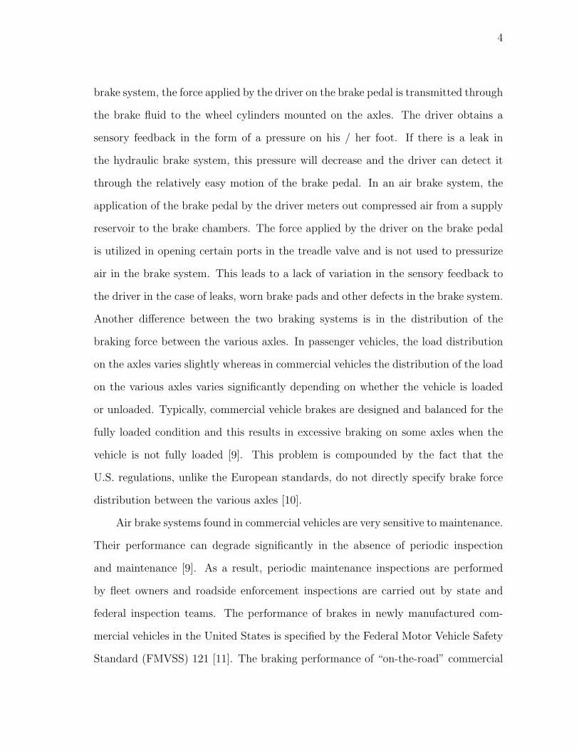
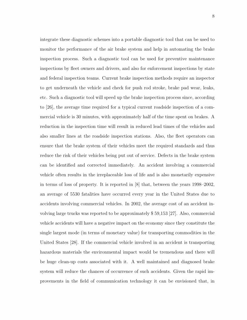
the near future an on-board diagnostic system may be used to remotely communicate

the status of the brake system to inspection stations in addition to providing the

same information to the driver, thereby facilitating real-time monitoring of vehicles

on roadways (see Fig. 1).

Fig. 1. An on-board diagnostic system for air brakes

C. Organization of this dissertation

A brief description of the air brake system currently used in commercial vehicles in the

United States will be provided in chapter II. The experimental facility constructed at

Texas A&M University for testing air brake systems will be presented in chapter III.

The details of the equipment used in the experimental setup will be provided in

this chapter. A model for predicting the pressure transients in a brake chamber

during the brake application process using the measurements of the treadle valve

plunger displacement and the supply pressure to the treadle valve will be derived in

chapter IV. In chapter V, a brief review of existing diagnostic tools for air brakes

will be presented and a scheme for automatically detecting leaks in the brake system

10

will be outlined. This scheme will be corroborated with experimental data and a

preliminary method for selecting thresholds for leak detection will be presented. Two

schemes for estimating the stroke of the push rod using the model for the pressure

transients in the brake chamber will be described in chapter VI. These schemes will

be corroborated with experimental data. Parameter estimation schemes for a class of

sequential hybrid systems will be developed in chapter VII and their performance will

be illustrated with examples. Chapter VIII presents concluding remarks and possible

scope for future work.

11

CHAPTER II

A BRIEF DESCRIPTION OF THE AIR BRAKE SYSTEM

Many mechanical systems have used and are using compressed air as their energy

transmitting medium. Compressed air is being employed in a wide spectrum of ap-

plications including – machine shop tools (such as drills, impact wrenches, grinders,

screwdrivers, tappers, nut runners, riveters, sand rammers, etc.), contractors’ tools 1

(such as road / pavement breakers and rock drills), mining and quarrying equipment,

air motors, material handling equipment (such as hoists, wrenches, cranes, conveyors,

agitators, etc.), paint spraying, marine applications, pneumatic actuators, etc. [29].

One of the major applications of compressed air in the field of transportation has

been in the development of the air brake system.

In the United States railway industry, air brake systems were initially introduced

during the nineteenth century. Before the introduction of the air brake system, railway

cars were retarded mainly by mechanical means (for example, by levers, chains and

other linkages) and were hand-operated by brakemen usually through the rotation of

a handwheel [30]. A variety of alternate braking systems were developed by many

individuals, but the first practically applicable air brake system was developed by

George Westinghouse when he introduced his “Straight Air Brake” in 1869 [31], [32].

Interesting accounts of this invention of Westinghouse and his further improvements

and additions to the air brake system can be found in [33] and [34]. A detailed

description of the evolution of the air brake system including the early mechanical

brakes, vacuum brakes and finally the air brake system can be found in [35]. A

review of various issues with these early train air brake systems can be found in [36].

1usually refers to equipments used in construction sites that are powered by com-pressed air.

12

A discussion of the development of different types of brakes including air brakes can

be found in [37].

Before providing a detailed description of the air brake system that is currently

used in commercial vehicles, a brief description of the air brake system used in trains

is presented.

A. The train air brake system

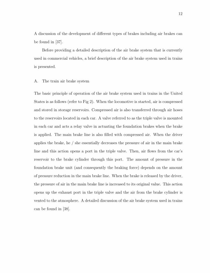
The basic principle of operation of the air brake system used in trains in the United

States is as follows (refer to Fig 2). When the locomotive is started, air is compressed

and stored in storage reservoirs. Compressed air is also transferred through air hoses

to the reservoirs located in each car. A valve referred to as the triple valve is mounted

in each car and acts a relay valve in actuating the foundation brakes when the brake

is applied. The main brake line is also filled with compressed air. When the driver

applies the brake, he / she essentially decreases the pressure of air in the main brake

line and this action opens a port in the triple valve. Then, air flows from the car’s

reservoir to the brake cylinder through this port. The amount of pressure in the

foundation brake unit (and consequently the braking force) depends on the amount

of pressure reduction in the main brake line. When the brake is released by the driver,

the pressure of air in the main brake line is increased to its original value. This action

opens up the exhaust port in the triple valve and the air from the brake cylinder is

vented to the atmosphere. A detailed discussion of the air brake system used in trains

can be found in [38].

13

Fig. 2. Principle of operation of the train brake system

B. The air brake system used in commercial vehicles

The wide use of air brake systems in commercial vehicles started mainly in the early

twentieth century. One of the earliest air brake systems for trucks was developed by

George Lane in 1919 [39]. The initial air brake system consisted of storage reservoirs,

control valves and brake chambers. As time progressed, the design of the air brake

system underwent modifications to include several features such as foot-operated

treadle valves, relay valves, spring brake chambers, tractor protection valves and

many more [39], [40]. A description of the modern air brake system including its

various components and their functioning can be found in [39].

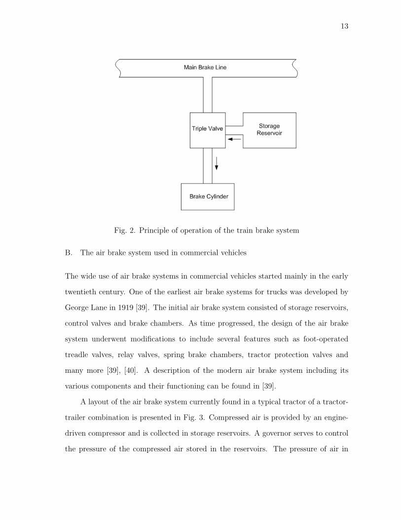
A layout of the air brake system currently found in a typical tractor of a tractor-

trailer combination is presented in Fig. 3. Compressed air is provided by an engine-

driven compressor and is collected in storage reservoirs. A governor serves to control

the pressure of the compressed air stored in the reservoirs. The pressure of air in

14

the storage reservoirs is typically maintained between 790.9 kPa (100 psig) and 997.7

kPa (130 psig). Compressed air is supplied from these reservoirs to the treadle and

relay valves. The driver applies the brake by pressing the brake pedal mounted on

the treadle valve. This action meters the compressed air from the supply ports of the

treadle valve to its delivery ports from where it travels through hoses to the brake

chambers mounted on the axles.

Fig. 3. A general layout of a tractor air brake system

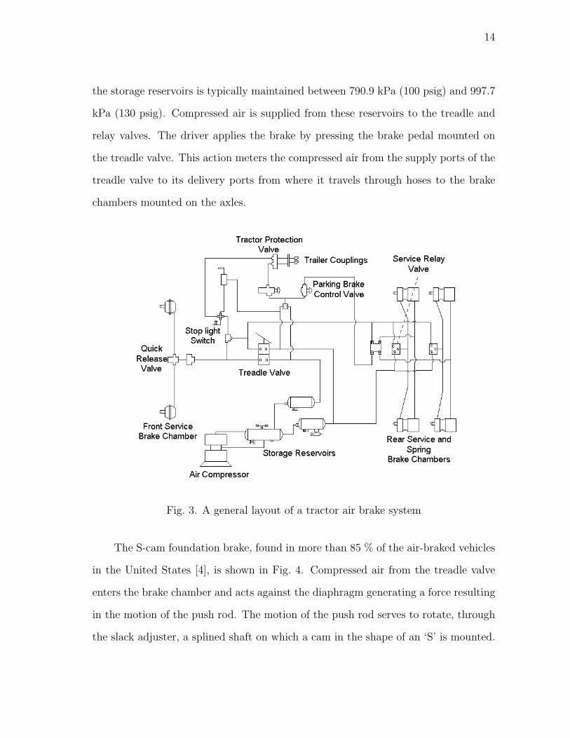
The S-cam foundation brake, found in more than 85 % of the air-braked vehicles

in the United States [4], is shown in Fig. 4. Compressed air from the treadle valve

enters the brake chamber and acts against the diaphragm generating a force resulting

in the motion of the push rod. The motion of the push rod serves to rotate, through

the slack adjuster, a splined shaft on which a cam in the shape of an ‘S’ is mounted.

15

The ends of two brake shoes rest on the profile of the S-cam and the rotation of the

S-cam pushes the brake shoes outwards so that the brake pads make contact with the

rotating drum. This action results in the deceleration of the rotating drum. When

the brake pedal is released by the driver, air is exhausted from the brake chamber to

the atmosphere causing the push rod to stroke back into the brake chamber and the

S-cam now rotates in the opposite direction. The contact between the brake pads

and the drum is now broken and the brake is thus released. A schematic of a drum

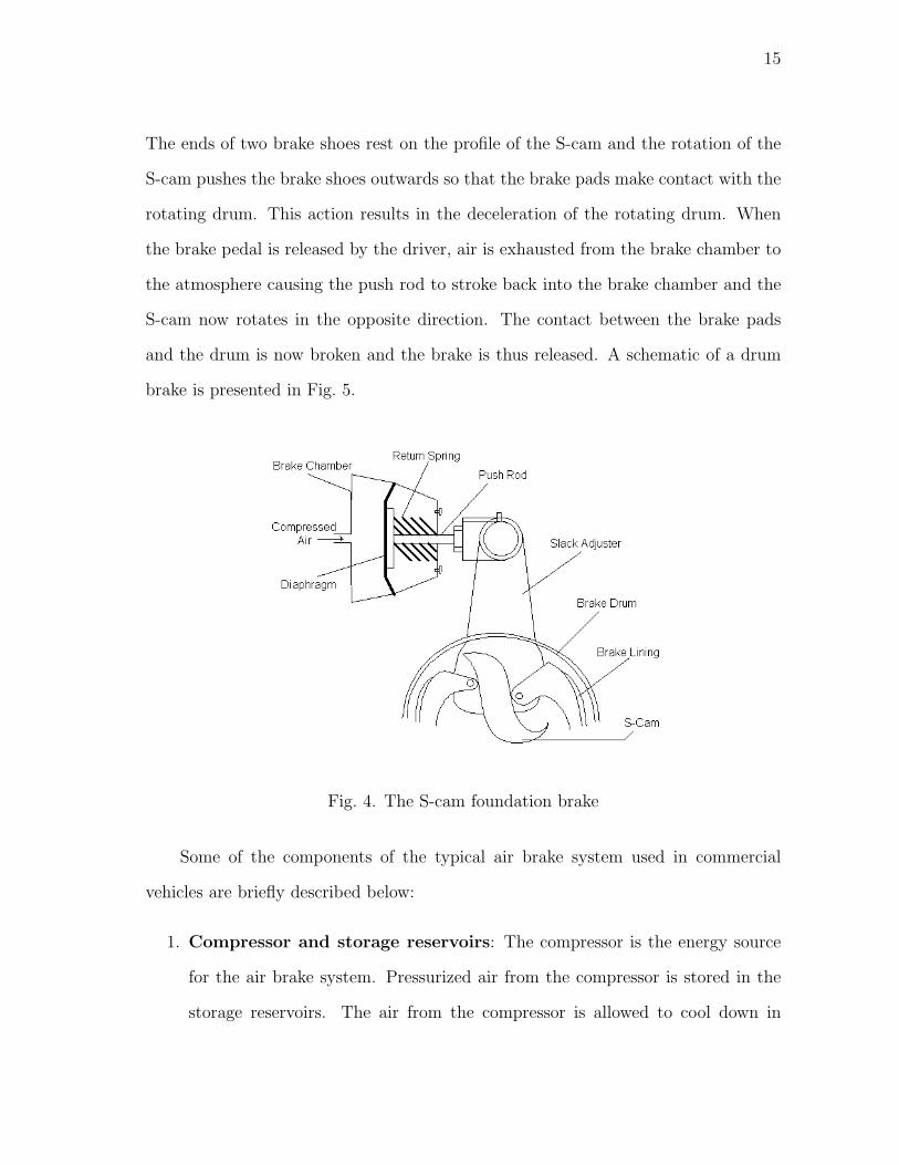
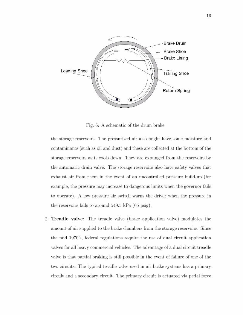
brake is presented in Fig. 5.

Fig. 4. The S-cam foundation brake

Some of the components of the typical air brake system used in commercial

vehicles are briefly described below:

1. Compressor and storage reservoirs: The compressor is the energy source

for the air brake system. Pressurized air from the compressor is stored in the

storage reservoirs. The air from the compressor is allowed to cool down in

16

Fig. 5. A schematic of the drum brake

the storage reservoirs. The pressurized air also might have some moisture and

contaminants (such as oil and dust) and these are collected at the bottom of the

storage reservoirs as it cools down. They are expunged from the reservoirs by

the automatic drain valve. The storage reservoirs also have safety valves that

exhaust air from them in the event of an uncontrolled pressure build-up (for

example, the pressure may increase to dangerous limits when the governor fails

to operate). A low pressure air switch warns the driver when the pressure in

the reservoirs falls to around 549.5 kPa (65 psig).

2. Treadle valve: The treadle valve (brake application valve) modulates the

amount of air supplied to the brake chambers from the storage reservoirs. Since

the mid 1970’s, federal regulations require the use of dual circuit application

valves for all heavy commercial vehicles. The advantage of a dual circuit treadle

valve is that partial braking is still possible in the event of failure of one of the

two circuits. The typical treadle valve used in air brake systems has a primary

circuit and a secondary circuit. The primary circuit is actuated via pedal force

17

and it provides compressed air to the brakes mounted on the rear axles of a

tractor and the secondary circuit acts like a relay valve in the sense that the

air delivered by the primary circuit is used to actuate it. The secondary circuit

provides air to the brake chambers on the front axle and in the event of failure

of the primary circuit, it is actuated directly by pedal force.

3. Quick release valve and relay valve: A quick release valve is mounted on

the front axle of the tractor and the air from the secondary circuit of the treadle

valve passes through it en route to the two front brake chambers. It facilitates

the quick exhaust of the air from the front brake chambers when the brake pedal

is released by the driver. A relay valve (referred to as a service relay valve in

Fig. 3) is mounted on the rear axles and obtains compressed air supply from the

storage reservoirs. The air from the primary circuit of the treadle valve enters

the control port of the relay valve and this action meters out compressed air to

the rear brake chambers. The relay valve also helps in the quick exhaust of air

from the rear brake chambers when the brake pedal is released by the driver.

4. Brake chambers: The brake chambers convert the energy from the pressurized

air into a mechanical force that displaces the push rod which in turn actuates

the foundation brakes. The push rod is used to rotate the S-cam (through the

slack adjuster) which in turn pushes the brake pads against the rotating drum.

A combination service brake / spring brake chamber mounted on the rear axles

functions as a service / emergency / parking brake. It has two chambers – one of

which acts as a normal service brake chamber and the other chamber is always

filled with pressurized air to hold back a power spring in a compressed state.

In the case of brake system failure or when the parking brakes are applied,

this chamber is drained out and the compressed power spring then pushes the

18

push rod thereby applying the brake. The specification of the brake chamber

is usually given in terms of its effective cross-sectional area. For example, a

“Type 20” brake chamber has a cross-sectional area of 20 in2. Type 20 brake

chambers are usually used on the front axle and “Type 30” brake chambers are

usually used on the rear axles of a commercial vehicle.

5. Automatic slack adjuster: A slack adjuster converts a translational motion of

the push rod into a rotation of the S-cam shaft. The output force from the brake

chambers decreases rapidly when the push rod stroke exceeds the re-adjustment

limit. Also, all the brakes in a tractor-trailer combination vehicle have to be

in proper adjustment relative to each other so that the net braking effort is

shared proportionally between all of them. Before the advent of automatic slack

adjusters, the brakes had to be manually adjusted by rotating an adjusting nut

which in turn rotated the S-cam through a worm shaft. During the late 1970’s

the use of automatic slack adjusters started and today their use is mandatory in

all commercial vehicles. An automatic slack adjuster transmits the braking force

from the push rod to the S-cam and also adjusts the brakes when the linings

wear out and / or the drum expands (which results in an increased clearance

between the brake pads and the brake drum).

6. Foundation brakes: These units are mounted on the axles and they act on

the rotating wheels thereby retarding the motion of the vehicle. Commercial

vehicles in the United States commonly use S-cam drum foundation brakes,

whereas in Europe disc brakes are slowly replacing drum brakes [39]. Disc brakes

offer lower sensitivity of the brake torque to the brake pad friction coefficient,

better fade resistance and improved brake efficiency when compared to drum

brakes. Their main limitation is the absence of “self-energization” [39] (this term

19

refers to the augmentation of the moment due to the actuation force acting on

the brake pad by the moment due to the friction force acting on the brake pad)

available in drum brakes resulting in the need for higher actuation air pressures

when compared to drum brakes. Comparisons between the performance of drum

and disc brakes can be found in [41], [42] and [43].

The above discussion presented a brief description of a few critical components

of the air brake system currently used in commercial vehicles. For a more detailed

description, the interested reader is referred to [39], [44] and [45]. A list of components

of the pneumatic subsystem and the mechanical subsystem is presented in Table I

and Table II respectively.

C. Improvements to the basic air brake system and emerging technologies

A description of the various components of the basic air brake system was presented

in the previous section. One of the most important improvements made to the air

brake system is the introduction of the Antilock Brake System (ABS). As the name

suggests this system prevents the wheels of a commercial vehicle from locking up (a

wheel is said to have locked up if it has stopped rotating when the vehicle is still in

motion) during the process of braking and thus improving the stability of the braking

process. The locking up of wheels on the front axle of a tractor-trailer combination

will result in the loss of steering control; the locking up of wheels on the rear axles

of a tractor may result in jackknifing; and the locking up of the wheels on the trailer

axles will result in trailer swing [39], [46]. Every single unit truck manufactured on or

after March 1, 1998 and every tractor manufactured after March 1, 1997 must have

an antilock brake system installed on them [11].

A typical ABS utilizes the measurement of wheel speeds and decreases the pres-

20

Table I. Components of the pneumatic subsystem of the air brake system

Component Description

Compressor Acts as the energy source providing compressed air.

Storage reser-

voirs

Store the compressed air and supply it to the treadle and relay

valves.

Safety valve Prevents an excessive pressure build-up in the storage reservoirs.

Drain valve Removes moisture and contaminants from the air stored in the

reservoirs.

Low air pres-

sure switch

Warns the driver when the pressure in the reservoirs falls to

around 65 psig.

Treadle valve Modulates the amount of air being supplied to the brake cham-

bers.

Quick release

valve

Releases the front brakes quickly.

Relay valve Regulates the brakes on the rear axles.

Parking brake

control valve

Located in the driver’s cab and is used to apply the parking

brakes.

Tractor pro-

tection valve

Protects the tractor brake system in the case of trailer break-

away and / or when there are severe leakages in the brake sys-

tem.

Trailer brake

control valve

Actuates the trailer brakes independent of the tractor brakes

and is applied by the driver.

21

Table II. Components of the mechanical subsystem of the air brake system

Component Description

Brake chamber Converts the energy provided by the compressed air into

a mechanical force.

Push rod Connected to the brake chamber diaphragm and trans-

mits the force to the slack adjuster.

Automatic slack ad-

juster

Converts the translational motion of the push rod into a

rotation of the S-cam.

S-cam Moves the brake pads during brake application and

presses them against the brake drum.

sure of air in the brake chambers if it senses an impending wheel lock up. The main

components of an ABS used in commercial vehicle include wheel speed sensors, an

electronic control unit to process the information from these sensors and modulator

valves that regulate the pressure in the brake chamber in the event of an impending

wheel lock up [39]. Detailed descriptions of ABS and various layouts of the same can

be found in [39], [44], [47], [48].

One of the emerging technologies for air brake systems is the Electronic Braking

System (EBS). An EBS generates an electric signal when the driver presses the brake

pedal and this electric signal is then provided to electro-pneumatic actuators that

are mounted near the foundation brakes. These actuators regulate the pressure of air

in the brake chambers in proportion to the magnitude of the electric signal received

by them [39]. It should be noted that the foundation brakes are still actuated by

compressed air. But the control signal to the relay valve is now an electric signal and

this leads to a reduction in both the number of pneumatic components and the time

22

lag between the brake pedal motion and the build up of pressure in the brake chamber

that exist in current air brake systems. This would lead to faster response times and

shorter stopping distances when compared with existing air brake systems [49], [50].

Also, an EBS results in an improved compatibility between the brakes on a tractor

and trailer since an electric signal is used to modulate the pressure in all the brake

chambers [49], [51]. If EBS is to be provided on existing commercial vehicles, it has

to be installed as a “redundant” system on top of the existing air brake system since

current regulations still require the existence of a complete air brake system [39].

23

CHAPTER III

THE EXPERIMENTAL SETUP

An experimental setup has been constructed at Texas A&M University that mir-

rors the actual air brake system currently used in commercial vehicles. A schematic

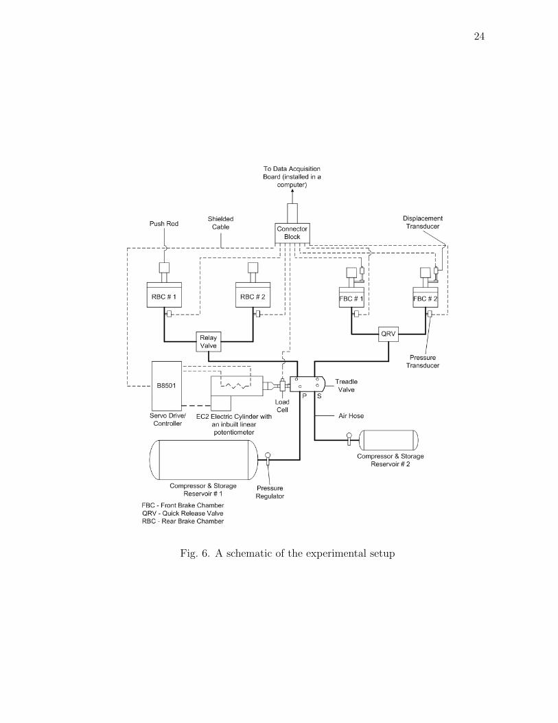
of this experimental setup is presented in Fig. 6. The various components of the

experimental setup can be broadly classified under three categories – brake system

components, actuation and motion control components and sensing and data acqui-

sition components. A brief description of each of these three categories is provided in

this chapter.

A. Brake system components

Two “Type-20” brake chambers (having an effective cross-sectional area of 20 in2) are

mounted on a front axle of a tractor and two “Type-30” brake chambers (having an

effective cross-sectional area of 30 in2) are mounted on a fixture designed to simulate

the rear axle of a tractor. The air supply to the two circuits of the brake system

is provided by means of two compressors and storage reservoirs. The reservoirs are

chosen such that their volume is more than twelve times the volume of the brake

chambers that they provide to, as required by FMVSS 121 [11], [52]. Pressure regula-

tors are mounted at the delivery ports of the reservoirs to control the supply pressure

to the treadle valve.

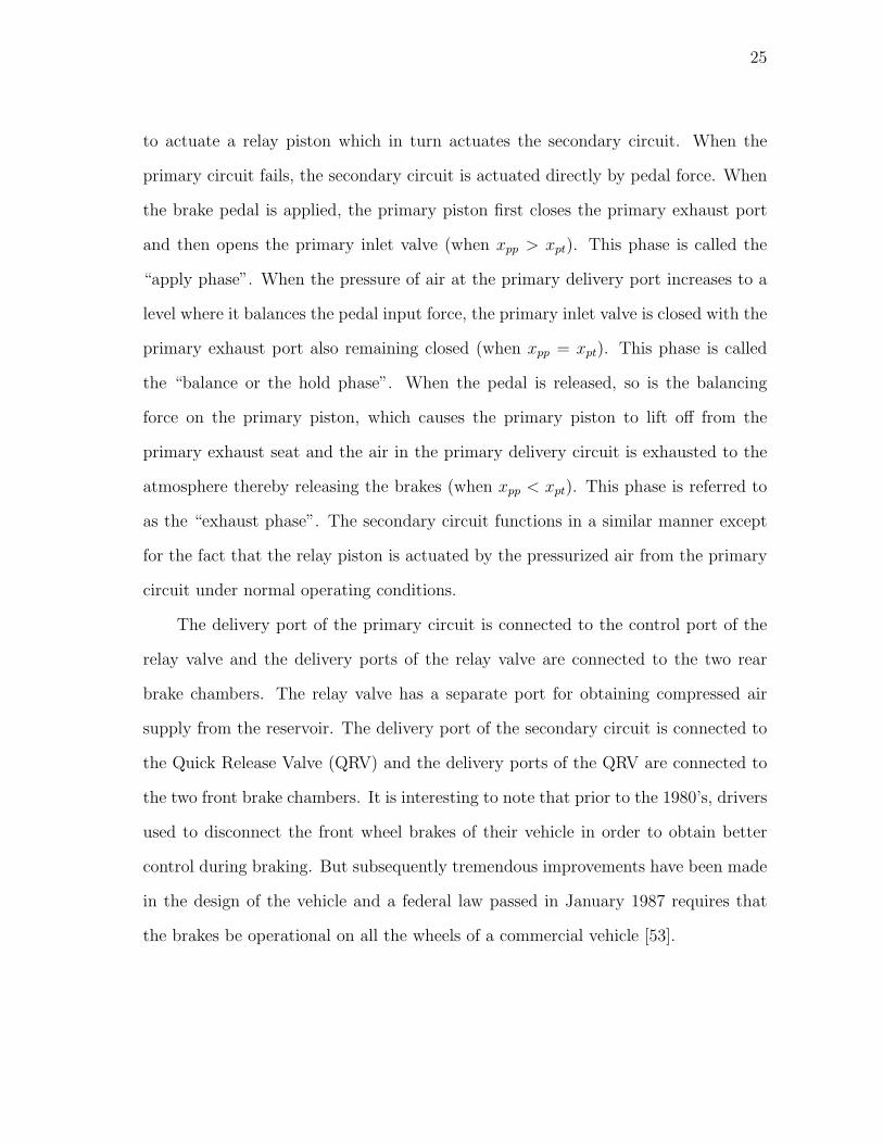
A cross-sectional view of the treadle valve used in the experiments is illustrated

in Fig. 7. The treadle valve consists of two circuits – the primary circuit and the

secondary circuit. The primary circuit is actuated by the force applied by the driver

on the brake pedal and the secondary circuit acts essentially as a relay valve. Under

normal operating conditions, pressurized air delivered by the primary circuit is used

24

Fig. 6. A schematic of the experimental setup

25

to actuate a relay piston which in turn actuates the secondary circuit. When the

primary circuit fails, the secondary circuit is actuated directly by pedal force. When

the brake pedal is applied, the primary piston first closes the primary exhaust port

and then opens the primary inlet valve (when xpp > xpt). This phase is called the

“apply phase”. When the pressure of air at the primary delivery port increases to a

level where it balances the pedal input force, the primary inlet valve is closed with the

primary exhaust port also remaining closed (when xpp = xpt). This phase is called

the “balance or the hold phase”. When the pedal is released, so is the balancing

force on the primary piston, which causes the primary piston to lift off from the

primary exhaust seat and the air in the primary delivery circuit is exhausted to the

atmosphere thereby releasing the brakes (when xpp < xpt). This phase is referred to

as the “exhaust phase”. The secondary circuit functions in a similar manner except

for the fact that the relay piston is actuated by the pressurized air from the primary

circuit under normal operating conditions.

The delivery port of the primary circuit is connected to the control port of the

relay valve and the delivery ports of the relay valve are connected to the two rear

brake chambers. The relay valve has a separate port for obtaining compressed air

supply from the reservoir. The delivery port of the secondary circuit is connected to

the Quick Release Valve (QRV) and the delivery ports of the QRV are connected to

the two front brake chambers. It is interesting to note that prior to the 1980’s, drivers

used to disconnect the front wheel brakes of their vehicle in order to obtain better

control during braking. But subsequently tremendous improvements have been made

in the design of the vehicle and a federal law passed in January 1987 requires that

the brakes be operational on all the wheels of a commercial vehicle [53].

26

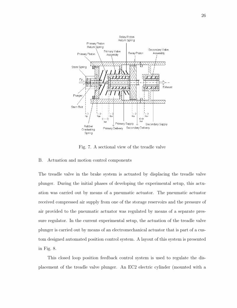
Fig. 7. A sectional view of the treadle valve

B. Actuation and motion control components

The treadle valve in the brake system is actuated by displacing the treadle valve

plunger. During the initial phases of developing the experimental setup, this actu-

ation was carried out by means of a pneumatic actuator. The pneumatic actuator

received compressed air supply from one of the storage reservoirs and the pressure of

air provided to the pneumatic actuator was regulated by means of a separate pres-

sure regulator. In the current experimental setup, the actuation of the treadle valve

plunger is carried out by means of an electromechanical actuator that is part of a cus-

tom designed automated position control system. A layout of this system is presented

in Fig. 8.

This closed loop position feedback control system is used to regulate the dis-

placement of the treadle valve plunger. An EC2 electric cylinder (mounted with a

27

Fig. 8. A layout of the treadle valve plunger position control system

B23 brushless servo motor) manufactured by Industrial Devices Corporation (IDC) /

Danaher Motion is used for actuation [54]. The actuator shaft is interfaced with the

servo motor through a belt drive and lead screw assembly. The actuator is controlled

by a B8501 Servo Drive / Controller [55], [56]. A linear potentiometer is inbuilt in the

electric cylinder and its output is provided to the servo drive. The servo drive also

receives a feedback signal from an encoder mounted on the motor shaft to regulate the

torque input to the motor. The desired plunger motion trajectory is provided from

the computer to the servo drive through the analog output channel of a Data Ac-

quisition (DAQ) board. The servo drive compares the difference between the desired

displacement and the measurement from the linear potentiometer at each instant in

time and provides the suitable control input to the actuator. The position control

system is tuned to obtain the desired performance using IDC’s Servo Tuner software

program [57]. A general overview of the processes of design and implementation of

motion control systems can be found in [58].

28

C. Sensing and data acquisition components

A pressure transducer is mounted at the entrance of each of the four brake chambers

by means of a custom designed and fabricated pitot tube fixture. A displacement

transducer is mounted on each of the two front brake chamber push rods through

appropriately fabricated fixtures in order to measure the push rod stroke. All the

transducers are interfaced with a connector block through shielded cables. The con-

nector block is connected to a PCI-MIO-16E-4 DAQ board [59] (mounted on a PCI

slot inside a desktop computer) that collects the data during experimental test runs.

This DAQ board can measure eight analog input signals in the differential mode and

can provide two analog output signals. The DAQ board discretizes the analog input

signals using an analog-to-digital (A/D) converter and the resulting digital signals

are stored in the computer. An application program written in MATLAB / Simulink

is used to collect and store the data in the computer. A discussion of various aspects

of data acquisition in general can be found in [60].

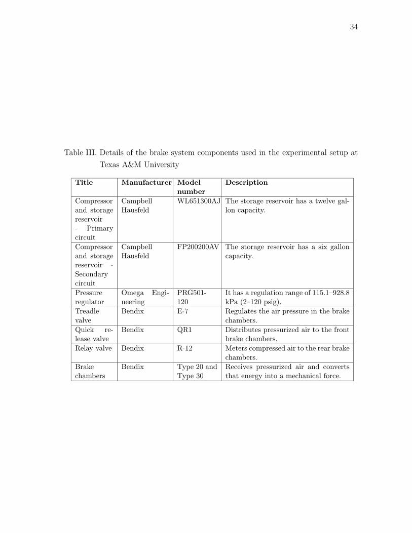
The specifications of the various brake system components used in the experimen-

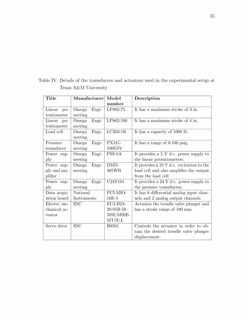
tal setup are summarized in Table III. The specifications of the various sensing and

actuation components used in the experimental setup are summarized in Table IV.

A few photographs of the experimental setup are presented in Figs. 9 to 13.

29

Fig. 9. The air brake experimental facility at Texas A&M University

30

Fig. 10. The front axle of a typical commercial vehicle

31

Fig. 11. The servo drive and the data acquisition system

32

Fig. 12. The electromechanical actuator and the treadle valve

33

Fig. 13. The pneumatic actuator and the treadle valve

34

Table III. Details of the brake system components used in the experimental setup at

Texas A&M University

Title Manufacturer Modelnumber

Description

Compressorand storagereservoir- Primarycircuit

CampbellHausfeld

WL651300AJ The storage reservoir has a twelve gal-lon capacity.

Compressorand storagereservoir -Secondarycircuit

CampbellHausfeld

FP200200AV The storage reservoir has a six galloncapacity.

Pressureregulator

Omega Engi-neering

PRG501-120

It has a regulation range of 115.1–928.8kPa (2–120 psig).

Treadlevalve

Bendix E-7 Regulates the air pressure in the brakechambers.

Quick re-lease valve

Bendix QR1 Distributes pressurized air to the frontbrake chambers.

Relay valve Bendix R-12 Meters compressed air to the rear brakechambers.

Brakechambers

Bendix Type 20 andType 30

Receives pressurized air and convertsthat energy into a mechanical force.

35

Table IV. Details of the transducers and actuators used in the experimental setup at

Texas A&M University

Title Manufacturer Modelnumber

Description

Linear po-tentiometer

Omega Engi-neering

LP802-75 It has a maximum stroke of 3 in.

Linear po-tentiometer

Omega Engi-neering

LP802-100 It has a maximum stroke of 4 in.

Load cell Omega Engi-neering

LC203-1K It has a capacity of 1000 lb.

Pressuretransducer

Omega Engi-neering

PX181-100G5V

It has a range of 0-100 psig.

Power sup-ply

Omega Engi-neering

PSS-5A It provides a 5 V d.c. power supply tothe linear potentiometers.

Power sup-ply and am-plifier

Omega Engi-neering

DMD-465WB

It provides a 10 V d.c. excitation to theload cell and also amplifies the outputfrom the load cell.

Power sup-ply

Omega Engi-neering

U24Y101 It provides a 24 V d.c. power supply tothe pressure transducers.

Data acqui-sition board

NationalInstruments

PCI-MIO-16E-4

It has 8 differential analog input chan-nels and 2 analog output channels.

Electro me-chanical ac-tuator

IDC EC2-B23-20-05B-50-MSI/MS6E-MT1E-L

Actuates the treadle valve plunger andhas a stroke range of 100 mm.

Servo drive IDC B8501 Controls the actuator in order to ob-tain the desired treadle valve plungerdisplacement.

36

CHAPTER IV

A MODEL FOR PREDICTING THE PRESSURE TRANSIENTS IN THE AIR

BRAKE SYSTEM

The first step in developing reliable model-based diagnostic schemes for air brake

systems is to develop a “fault-free” model (one that describes the response of the

system under the absence of faults in the system) for the same. It has been found

out from experiments that observing the pressure transients in the brake chambers

of the air brake system during the brake application process will help in monitoring

the brake system for leaks and out-of-adjustment. Hence, a model for predicting the

pressure transients in a brake chamber of the air brake system has been developed and

presented in [23]. This model correlates the pressure in the brake chamber with the

treadle valve plunger displacement and the supply pressure to the treadle valve. In

this chapter, a brief description of the model is provided and the governing equations

of the model are summarized. Improvements have been made to this model and these

are also presented.

A. Existing models for air brake systems

The hydraulic brake system has been extensively studied and models for the same

have been developed by many authors. Gerdes et al. [61] developed a model for a

hydraulic brake system with a vacuum booster. They combined a static valve model

with equations of air flow within the booster. Khan et al. [62] used bond graph

techniques to develop models for the booster, the master cylinder and the wheel

cylinder. In both cases, the authors measured the wheel cylinder chamber pressure as

a function of time and attempted to predict the pressure transients with their models.

In [63], the author has developed an overall model for the hydraulic brake system by

37

presenting individual models for each major component of the brake system.

A large number of published works on models for air brake systems relate quanti-

ties such as brake force, vehicle deceleration, brake pad temperature and brake torque

with the brake chamber pressure and the push rod stroke [64], [65], [66], [15]. Such

models essentially characterize the mechanical subsystem of the air brake system. It

is also important to develop models that predict the pressure transients in the brake

system since such models can check the brake “rise times” and compare them with

the values specified by FMVSS 121 to ensure the proper operation of the brake sys-

tem. The maximum brake force developed in a given brake application depends on

the steady state brake chamber pressure and a model for the pneumatic subsystem

is necessary to predict the same. Also, the estimation of stopping distances from

measurements of brake force requires the values of air pressure buildup / rise times

which can be obtained from a model of the pressure transients.

It has been observed in experiments that the occurrence of leaks and out-of-

adjustment of push rods are reflected on the pressure transients in the brake cham-

ber. Hence, a model for the pressure transients provides a way to develop diagnostic

schemes for the air brake system. Acarman et al. [67] presented a model for the

pressure transients in air brakes with an Antilock Braking System (ABS). Dunn et

al. [68] modeled the pressure transients using a first order linear ordinary differential

equation with the associated “time constants” obtained from experimental data. A

similar model has been developed by Kandt et al. [69] for the pressure transients

during brake release. These models do not explicitly take into account the mechanics

of operation of the treadle valve.

38

B. A model for predicting the pressure transients in the brake chamber

The model presented in [23] takes into account the mechanics of operation of the

treadle valve and the flow of air in the brake system. A lumped parameter approach

has been adopted to model the pneumatic subsystem of the air brake system. The

configuration of the air brake system considered in this dissertation is the one where

the delivery port of the primary circuit is directly connected to one of the two front

brake chambers. This configuration will be considered for this first study of developing

model-based diagnostic schemes for air brakes based on the pressure transients in the

brake chamber.

1. Equations governing the mechanics of operation of the treadle valve

In this sub-section, the equations governing the motion of the components in the

primary circuit of the treadle valve (refer to Fig. 7) are presented. The operation of

the treadle valve has been described in section A of chapter III. The primary inlet

valve opening in the treadle valve has been modeled as a nozzle. The friction at the

sliding surfaces of the treadle valve is assumed to be negligible since these surfaces

are well lubricated. The springs in the treadle valve have been tested and found

to be linear in the region of their operation (except the rubber graduating spring).

Geometric parameters such as areas, initial deflections, etc., were also measured and

used in the following equations. The force applied by the driver on the brake pedal is

transmitted through the rubber graduating spring to the primary piston which then

opens the primary inlet valve. The governing equation of the primary piston during

the apply and hold phases of the brake application process is given by

(Mpp + Mpv)

(d2xpp(t)

dt2

)+ K2xpp(t) = Kssxp(t) + Fgs(t) + F1

−Ppd(t)(App − Apv) − PpsApv1 + PatmApp, (4.1)

39

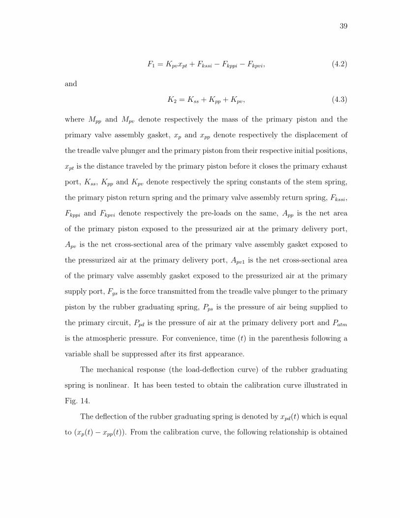
F1 = Kpvxpt + Fkssi − Fkppi − Fkpvi, (4.2)

and

K2 = Kss + Kpp + Kpv, (4.3)

where Mpp and Mpv denote respectively the mass of the primary piston and the

primary valve assembly gasket, xp and xpp denote respectively the displacement of

the treadle valve plunger and the primary piston from their respective initial positions,

xpt is the distance traveled by the primary piston before it closes the primary exhaust

port, Kss, Kpp and Kpv denote respectively the spring constants of the stem spring,

the primary piston return spring and the primary valve assembly return spring, Fkssi,

Fkppi and Fkpvi denote respectively the pre-loads on the same, App is the net area

of the primary piston exposed to the pressurized air at the primary delivery port,

Apv is the net cross-sectional area of the primary valve assembly gasket exposed to

the pressurized air at the primary delivery port, Apv1 is the net cross-sectional area

of the primary valve assembly gasket exposed to the pressurized air at the primary

supply port, Fgs is the force transmitted from the treadle valve plunger to the primary

piston by the rubber graduating spring, Pps is the pressure of air being supplied to

the primary circuit, Ppd is the pressure of air at the primary delivery port and Patm

is the atmospheric pressure. For convenience, time (t) in the parenthesis following a

variable shall be suppressed after its first appearance.

The mechanical response (the load-deflection curve) of the rubber graduating

spring is nonlinear. It has been tested to obtain the calibration curve illustrated in

Fig. 14.

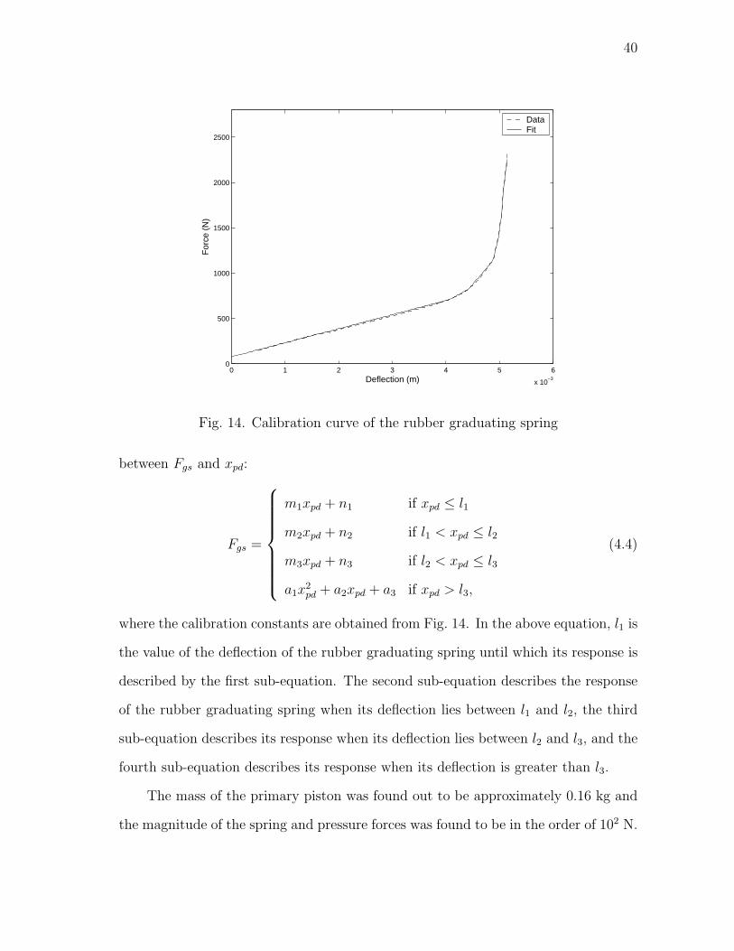
The deflection of the rubber graduating spring is denoted by xpd(t) which is equal

to (xp(t) − xpp(t)). From the calibration curve, the following relationship is obtained

40

0 1 2 3 4 5 6

x 10−3

0

500

1000

1500

2000

2500

Deflection (m)

For

ce (

N)

DataFit

Fig. 14. Calibration curve of the rubber graduating spring

between Fgs and xpd:

Fgs =

m1xpd + n1 if xpd ≤ l1

m2xpd + n2 if l1 < xpd ≤ l2

m3xpd + n3 if l2 < xpd ≤ l3

a1x2pd + a2xpd + a3 if xpd > l3,

(4.4)

where the calibration constants are obtained from Fig. 14. In the above equation, l1 is

the value of the deflection of the rubber graduating spring until which its response is

described by the first sub-equation. The second sub-equation describes the response

of the rubber graduating spring when its deflection lies between l1 and l2, the third

sub-equation describes its response when its deflection lies between l2 and l3, and the

fourth sub-equation describes its response when its deflection is greater than l3.

The mass of the primary piston was found out to be approximately 0.16 kg and

the magnitude of the spring and pressure forces was found to be in the order of 102 N.

41

Thus, the acceleration required for the inertial forces to be comparable with the spring

force and the pressure force terms has to be in the order of 102 − 103 m/s2, which is

not the case. Hence the inertial forces are neglected and Eq. (4.1) reduces to

K2xpp = Kssxp + Fgs + F1 − Ppd(App − Apv)

−PpsApv1 + PatmApp. (4.5)

During the exhaust phase, the equation of motion of the primary piston can be

written as

Mpp

(d2xpp

dt2

)= Fgs + Fkssi + Kss(xp − xpp) − (Ppd − Patm)App

−Kppxpp − Fkppi. (4.6)

It should be noted that at the start of the exhaust phase xpp is equal to xpt and

decreases as the exhaust phase progresses. Neglecting the inertia of the primary

piston the above equation can be simplified to

K3xpp = Kssxp + Fgs + F2 − PpdApp + PatmApp, (4.7)

where

F2 = Fkssi − Fkppi, (4.8)

K3 = Kss + Kpp. (4.9)

A detailed derivation of the model is presented in [23]. The equations of mo-

tion governing the operation of the secondary circuit of the treadle valve have been

similarly derived and presented in [23].

42

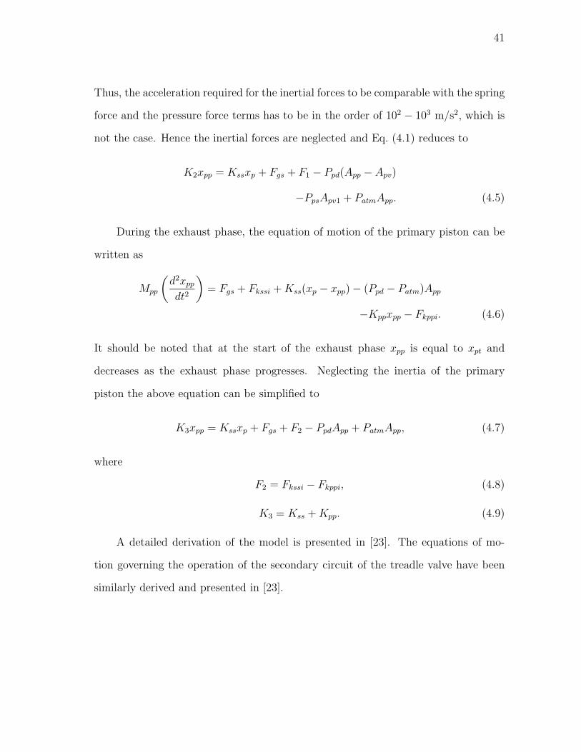
2. Equations governing the flow of air in the pneumatic subsystem of the brake

system

The primary inlet opening in the treadle valve serves as a channel through which

compressed air from the storage reservoirs flows to the brake chambers connected

to the delivery port of the primary circuit. This opening has been modeled as a

nozzle. For the flow through a restriction, if the ratio of the cross-sectional area of

the upstream section to the cross-sectional area of the restriction is 4.4 or higher, the

approach velocity to this restriction can be neglected and the upstream properties

(such as pressure, enthalpy, temperature, etc.) can be taken to be the upstream total

or stagnation properties [70]. In this application, the minimum ratio of the cross-

sectional area of the supply chamber of the treadle valve to the cross-sectional area

of the primary inlet opening (the restriction in this case) was found out to be around

15.4. Also, the cross-sectional area of the valve opening decreases monotonically to

a minimum value. Hence, the valve opening can be considered as a nozzle and the

properties in the supply chamber of the treadle valve can be taken as the stagnation

properties at the inlet section of the nozzle. It is assumed that the flow through this

valve opening is one-dimensional and isentropic. Further, it is assumed that the fluid

properties are uniform at all sections in the nozzle and air is assumed to behave like

an ideal gas with constant specific heats.

Under the above assumptions, the part of the pneumatic subsystem under con-

sideration can be visualized as illustrated in Fig. 15. It should be noted that when

the primary delivery port is connected directly to a front brake chamber, the term

Ppd in the above equations is taken to be the same as the pressure in the brake cham-

ber (denoted by Pb). For this configuration, the supply pressure term, denoted by

Pps in the above equations, is denoted by Po in the equations that follow.

43

Fig. 15. The simplified pneumatic subsystem under consideration

The brake chamber and the hose connecting the delivery port of the primary

circuit to it are lumped together and taken as the control volume under considera-

tion (see Fig. 16). The assumption that air can be modeled as an ideal gas provides

the following relationship [23]:

mb(t) =

(1

γ

)Pb(t)Vb(t)

RTb(t)+

Pb(t)Vb(t)

RTb(t), (4.10)

where mb is the mass of air in the control volume at any instant of time, Vb is the

volume of air in the control volume at that instant of time, Tb is the temperature of

air in the control volume at that instant of time and R is the gas constant of air. The

dot in the above equation represents the derivative with respect to time.

During the brake application process, the volume of air in the brake chamber (re-

fer to Fig. 17 for a cross-sectional view of the same) varies due to the fact that the

push rod strokes out of the brake chamber. In [23], the following relationship was

44

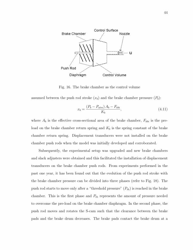
Fig. 16. The brake chamber as the control volume

assumed between the push rod stroke (xb) and the brake chamber pressure (Pb):

xb =(Pb − Patm) Ab − Fkbi

Kb

, (4.11)

where Ab is the effective cross-sectional area of the brake chamber, Fkbi is the pre-

load on the brake chamber return spring and Kb is the spring constant of the brake

chamber return spring. Displacement transducers were not installed on the brake

chamber push rods when the model was initially developed and corroborated.

Subsequently, the experimental setup was upgraded and new brake chambers

and slack adjusters were obtained and this facilitated the installation of displacement

transducers on the brake chamber push rods. From experiments performed in the

past one year, it has been found out that the evolution of the push rod stroke with

the brake chamber pressure can be divided into three phases (refer to Fig. 18). The

push rod starts to move only after a “threshold pressure” (Pth) is reached in the brake

chamber. This is the first phase and Pth represents the amount of pressure needed

to overcome the pre-load on the brake chamber diaphragm. In the second phase, the

push rod moves and rotates the S-cam such that the clearance between the brake

pads and the brake drum decreases. The brake pads contact the brake drum at a

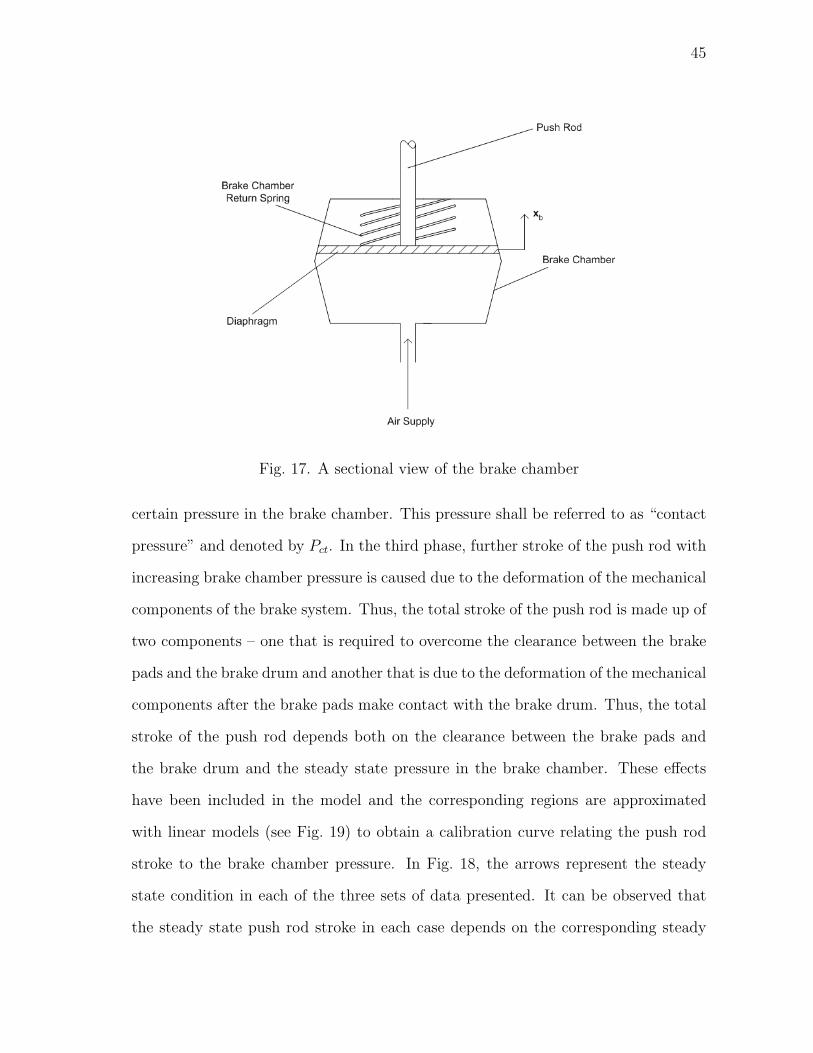
45

Fig. 17. A sectional view of the brake chamber

certain pressure in the brake chamber. This pressure shall be referred to as “contact

pressure” and denoted by Pct. In the third phase, further stroke of the push rod with

increasing brake chamber pressure is caused due to the deformation of the mechanical

components of the brake system. Thus, the total stroke of the push rod is made up of

two components – one that is required to overcome the clearance between the brake

pads and the brake drum and another that is due to the deformation of the mechanical

components after the brake pads make contact with the brake drum. Thus, the total

stroke of the push rod depends both on the clearance between the brake pads and

the brake drum and the steady state pressure in the brake chamber. These effects

have been included in the model and the corresponding regions are approximated

with linear models (see Fig. 19) to obtain a calibration curve relating the push rod

stroke to the brake chamber pressure. In Fig. 18, the arrows represent the steady

state condition in each of the three sets of data presented. It can be observed that

the steady state push rod stroke in each case depends on the corresponding steady

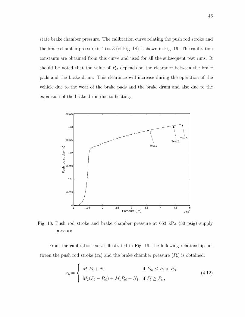
46

state brake chamber pressure. The calibration curve relating the push rod stroke and

the brake chamber pressure in Test 3 (of Fig. 18) is shown in Fig. 19. The calibration

constants are obtained from this curve and used for all the subsequent test runs. It

should be noted that the value of Pct depends on the clearance between the brake

pads and the brake drum. This clearance will increase during the operation of the

vehicle due to the wear of the brake pads and the brake drum and also due to the

expansion of the brake drum due to heating.

1 1.5 2 2.5 3 3.5 4 4.5 5

x 105

0

0.005

0.01

0.015

0.02

0.025

0.03

0.035

Pressure (Pa)

Pus

h ro

d st

roke

(m

) Test 1

Test 2 Test 3

Fig. 18. Push rod stroke and brake chamber pressure at 653 kPa (80 psig) supply

pressure

From the calibration curve illustrated in Fig. 19, the following relationship be-

tween the push rod stroke (xb) and the brake chamber pressure (Pb) is obtained:

xb =

M1Pb + N1 if Pth ≤ Pb < Pct

M2(Pb − Pct) + M1Pct + N1 if Pb ≥ Pct,(4.12)

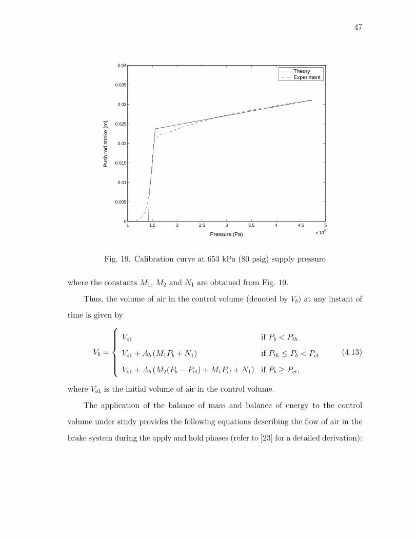
47

1 1.5 2 2.5 3 3.5 4 4.5 5

x 105

0

0.005

0.01

0.015

0.02

0.025

0.03

0.035

0.04

Pressure (Pa)

Pus

h ro

d st

roke

(m

)

TheoryExperiment

Fig. 19. Calibration curve at 653 kPa (80 psig) supply pressure

where the constants M1, M2 and N1 are obtained from Fig. 19.

Thus, the volume of air in the control volume (denoted by Vb) at any instant of

time is given by

Vb =

Vo1 if Pb < Pth

Vo1 + Ab (M1Pb + N1) if Pth ≤ Pb < Pct

Vo1 + Ab (M2(Pb − Pct) + M1Pct + N1) if Pb ≥ Pct,

(4.13)

where Vo1 is the initial volume of air in the control volume.

The application of the balance of mass and balance of energy to the control

volume under study provides the following equations describing the flow of air in the

brake system during the apply and hold phases (refer to [23] for a detailed derivation):

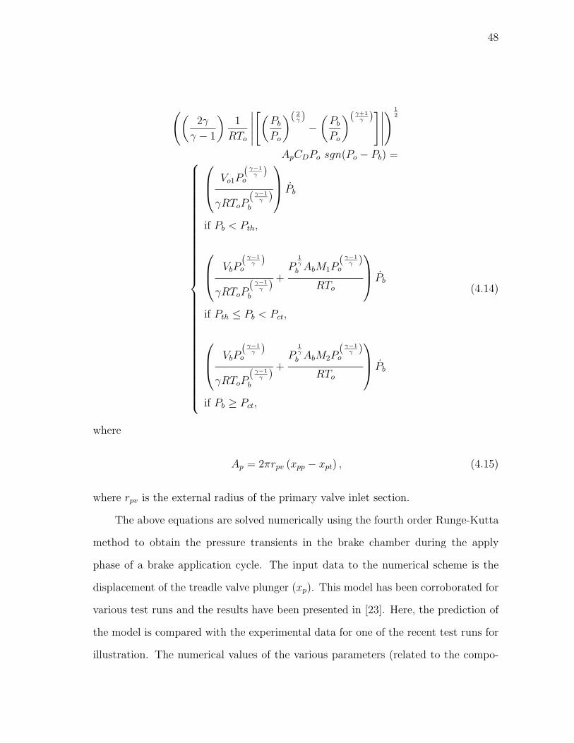
48

((2γ

γ − 1

)1

RTo

∣∣∣∣∣[(

Pb

Po

)( 2γ )

−(

Pb

Po

)( γ+1γ )

]∣∣∣∣∣) 1

2

ApCDPo sgn(Po − Pb) =

Vo1P

( γ−1γ )

o

γRToP( γ−1

γ )b

Pb

if Pb < Pth,

VbP

( γ−1γ )

o

γRToP( γ−1

γ )b

+P

1γ

b AbM1P( γ−1

γ )o

RTo

Pb

if Pth ≤ Pb < Pct,

VbP

( γ−1γ )

o

γRToP( γ−1

γ )b

+P

1γ

b AbM2P( γ−1

γ )o

RTo

Pb

if Pb ≥ Pct,

(4.14)

where

Ap = 2πrpv (xpp − xpt) , (4.15)

where rpv is the external radius of the primary valve inlet section.

The above equations are solved numerically using the fourth order Runge-Kutta

method to obtain the pressure transients in the brake chamber during the apply

phase of a brake application cycle. The input data to the numerical scheme is the

displacement of the treadle valve plunger (xp). This model has been corroborated for

various test runs and the results have been presented in [23]. Here, the prediction of

the model is compared with the experimental data for one of the recent test runs for

illustration. The numerical values of the various parameters (related to the compo-

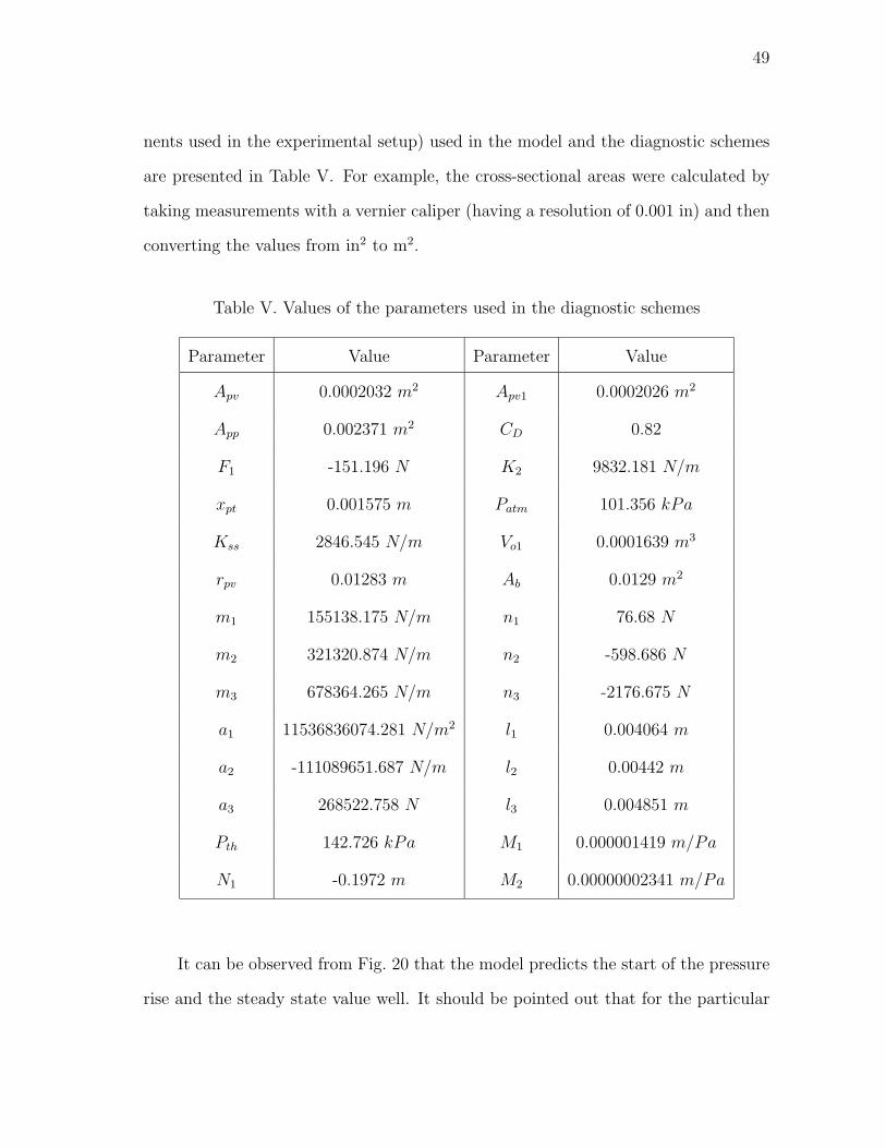
49

nents used in the experimental setup) used in the model and the diagnostic schemes

are presented in Table V. For example, the cross-sectional areas were calculated by

taking measurements with a vernier caliper (having a resolution of 0.001 in) and then

converting the values from in2 to m2.

Table V. Values of the parameters used in the diagnostic schemes

Parameter Value Parameter Value

Apv 0.0002032 m2 Apv1 0.0002026 m2

App 0.002371 m2 CD 0.82

F1 -151.196 N K2 9832.181 N/m

xpt 0.001575 m Patm 101.356 kPa

Kss 2846.545 N/m Vo1 0.0001639 m3

rpv 0.01283 m Ab 0.0129 m2

m1 155138.175 N/m n1 76.68 N

m2 321320.874 N/m n2 -598.686 N

m3 678364.265 N/m n3 -2176.675 N

a1 11536836074.281 N/m2 l1 0.004064 m

a2 -111089651.687 N/m l2 0.00442 m

a3 268522.758 N l3 0.004851 m

Pth 142.726 kPa M1 0.000001419 m/Pa

N1 -0.1972 m M2 0.00000002341 m/Pa

It can be observed from Fig. 20 that the model predicts the start of the pressure

rise and the steady state value well. It should be pointed out that for the particular

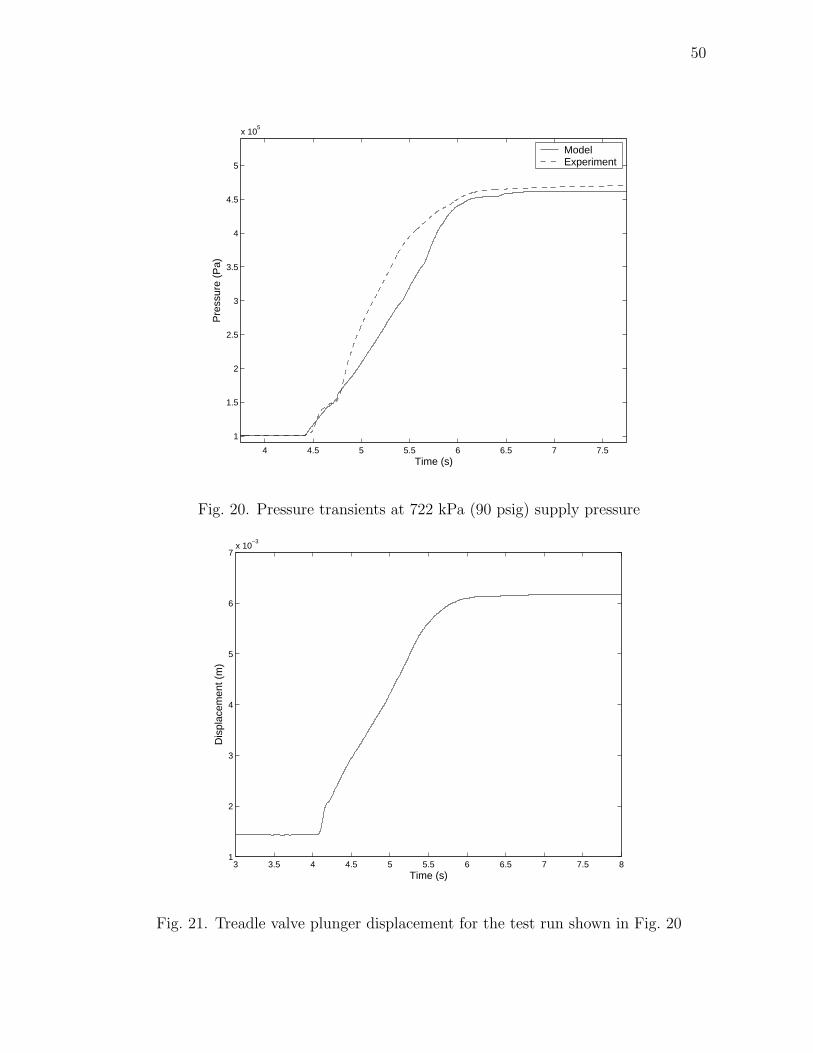
50

4 4.5 5 5.5 6 6.5 7 7.5

1

1.5

2

2.5

3

3.5

4

4.5

5

x 105

Time (s)

Pre

ssur

e (P

a)

ModelExperiment

Fig. 20. Pressure transients at 722 kPa (90 psig) supply pressure

3 3.5 4 4.5 5 5.5 6 6.5 7 7.5 81

2

3

4

5

6

7x 10

−3

Time (s)

Dis

plac

emen

t (m

)

Fig. 21. Treadle valve plunger displacement for the test run shown in Fig. 20

51

3 3.5 4 4.5 5 5.5 6 6.5 7 7.5 80

5x 10

5

Time (s)

Pre

ssur

e (P

a), s

olid

line

3 3.5 4 4.5 5 5.5 6 6.5 7 7.5 8

0

0.05

Pus

h ro

d st

roke

(m

), d

ashe

d lin

e

Fig. 22. Pressure and push rod stroke measurements for the test run shown in Fig. 20

test run illustrated in this figure, the brake application is started at approximately

t = 4.1 s (refer to Fig. 21). The value t = 0 s corresponds to the instant of time

at which the computer program for collecting the data is started. Also, note that

the second phase of the pressure transients (where there is a decrease in the slope of

the pressure growth curve) is also captured. One of the assumptions that was made

in deriving the model is that the second phase of the pressure transients is caused

by the increase in the volume of the brake chamber due to the stroke of the push

rod. This assumption is supported with the data presented in Fig. 22. Here, the

measured brake chamber pressure and push rod stroke have been plotted for the test

run illustrated in Fig. 20. It can be observed that the majority of the push rod stroke

falls in the second phase of the pressure growth curve. The latter part of the push rod

stroke is due to the deformation of the brake pads and other mechanical components

52

as the brake lining contacts the brake drum and is pressed against it.

This model will be the basis for the diagnostic schemes developed in this disser-

tation. To summarize, the main features of this model include the following:

1. This model considers both the mechanics of operation of the treadle valve and

the flow of air in the brake system to predict the pressure transients in the brake

chamber.

2. There is a time lag between the start of brake pedal application and the incep-

tion of pressure increase in the brake chamber. This effect is captured well by

this model through the equations governing the mechanics of operation of the

treadle valve.

3. The steady state brake chamber pressure depends on the supply pressure and

the steady state plunger displacement. This is also predicted reasonably well

by the model for a wide range of supply pressures and brake applications.

4. There are three modes / phases in the evolution of the brake chamber pressure

during the brake application process. In the first mode, due to pre-loads on

the push rod, it is stationary until the pressure increases to a threshold value.

Once this happens, a transition occurs to the second mode where the push rod

strokes out and the clearance between the brake pads and the brake drum starts

to decrease. During this mode the volume of the brake chamber increases and

the time rate of pressure increase falls down when compared with that of the

first mode. Once the brake pads contact the brake drum a transition is made to

the third mode and the pressure then increases to the steady state value. These

physically observed effects are included in the model and are captured by the

same.

53

C. The air brake system as an example of a sequential hybrid system

The response of the pneumatic subsystem of the air brake system is such that it can

be classified as what is usually referred to as an “Sequential Hybrid System”. In

this dissertation, the term “hybrid systems” is used to denote those systems whose

mathematical representation involves a finite set of governing ordinary differential

equations corresponding to a finite set of modes of operation. The mathematical

representation of a hybrid system is referred to as its “hybrid model”. The governing

equation in each mode is different and the transition / switch from one mode to

another occurs when some conditions involving one or more of the following – system’s

states, inputs, outputs, system parameters, etc., are satisfied. These conditions are

referred to as “transition / switch conditions”. These conditions may be known a

priori or unknown. In a sequential hybrid system, the possible modes are ordered

in a specific sequence. From a given mode, there can be only one forward transition

to the next mode in this ordered set or one backward transition to the previous

mode. Thus, the system can switch from a given mode to either the previous mode

or the following mode. Some examples of physical systems that exhibit this behavior

include the automatic transmission system in vehicles [1], multi-stage valves [71], [72],

air brake system, etc.

Many automotive systems have recently been described by hybrid models. Bal-

luchi et al. [73] have proposed a hybrid model for the automotive engine and power-

train that takes into account the four strokes of the pistons in the engine cylinders.

They use this hybrid model to develop a variety of engine controllers. Borrelli et

al. [74] have used a linearized hybrid vehicle model to develop traction control sys-

tems. Traction control systems improve the driver’s ability to control the vehicle

under wet and / or icy road conditions. Altafini et al. [75] have developed a lin-

54

earized hybrid model for the motion of a miniature tractor-trailer combination along

straight line and circular arc trajectories. In [76], the authors have developed a hybrid

model for the drive-line of an automotive power-train and designed observers based

on this model.

There are three modes of operation in the pneumatic subsystem of the air brake

system (refer to Eq.(4.14)) when the brake is applied. In ‘Mode 1’, the pressure in the

brake chamber (Pb) increases to Pth. In ‘Mode 2’, the push rod starts to move with

further increase in pressure and the clearance between the brake pads and the brake

drum starts to decrease. When the brake chamber pressure is equal to Pct, the brake

pads touch the brake drum and ‘Mode 3’ begins with further increase in pressure. In

this mode, the stroke of the push rod increases with pressure due to the deformation

of the mechanical components of the brake system. These three modes are illustrated

in Fig. 23.

The following features of the model should be noted:

1. The governing equation in each mode for each brake chamber is a nonlinear first

order ordinary differential equation in Pb and also it is different in each mode.

2. The transition conditions from one mode to another are linear equalities / in-

equalities involving the state (Pb), a known parameter (Pth) and an unknown

parameter (Pct). Thus, the transition condition between Mode 2 and Mode 3 is

not known. But the range of values of Pct is known from the possible range of

values of the push rod stroke.

3. Hence, a transition detection problem and a parameter estimation problem have

to be solved simultaneously. Also, the governing equations in Mode 3 involve

the unknown parameter (Pct).

This hybrid model for predicting the pressure transients in the air brake system

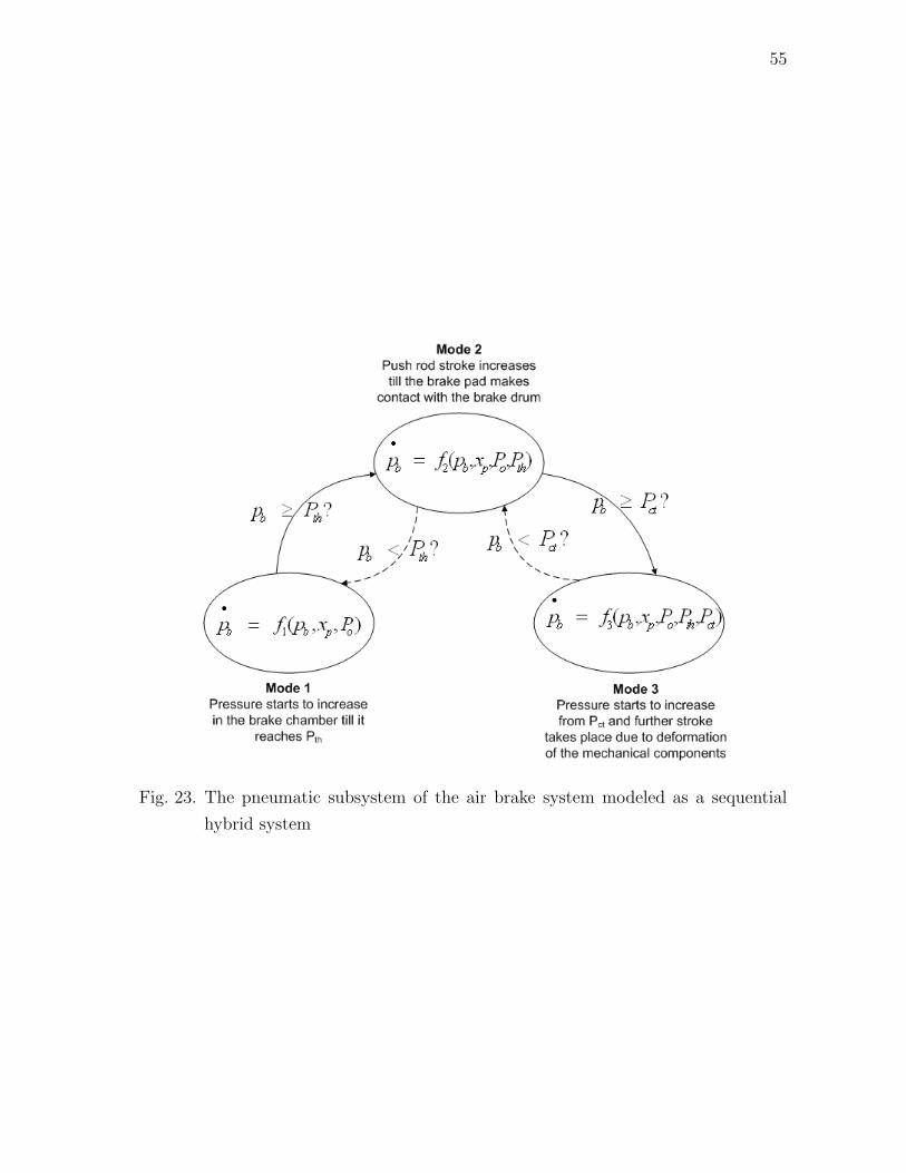
55

Fig. 23. The pneumatic subsystem of the air brake system modeled as a sequential

hybrid system

56

will be used to develop schemes for estimating the push rod stroke. It shall be

observed shortly that the problem of estimating the push rod stroke can be posed as a

parameter estimation problem and a transition detection problem involving the hybrid

model presented in this section. The problems of transition detection and parameter

estimation in such classes of nonlinear sequential hybrid systems are currently open.

D. A brief discussion concerning controlling the pressure in the air brake system

A cruise control system is a standard feature in most of the automobiles on the road

today. It maintains the vehicle speed to the value set by the driver by automatically

regulating the engine throttle [77], [78]. A sensor that measures the vehicle speed is

used to provide the feedback signal to this system. A cruise control system is usually

activated by the driver when the vehicle is traveling at medium / high speeds in

smoothly flowing traffic. A conventional cruise control system utilizes a Proportional-

Integral-Derivative (PID) controller to minimize the error between the desired and

the measured vehicle speed [79].

In recent years, studies have been carried out to develop “Adaptive Cruise Con-

trol” (ACC) systems or “Autonomous Intelligent Cruise Control” (AICC) systems.

The objective of these systems is to maintain a constant distance between two consec-

utive vehicles by controlling the engine throttle and the brake system. These systems

obtain the spacing between vehicles from sensors such as a radar mounted on the

vehicle [80]. They are being developed so that they can be engaged at low speeds

in moderate to heavy traffic conditions to automatically control the motion of the

vehicle in a safe manner. Studies have been recently carried out to evaluate and

implement these systems on vehicles [81], [82], [83].

While most of the research on ACC has focused on passenger cars, the benefits

57

of implementing this system on heavy trucks have far reaching consequences [84]. A

typical ACC system for heavy trucks controls the engine throttle, the transmission and

the brake system and will be interfaced with existing systems like the Antilock Braking

System (ABS), Traction Control System (TCS), etc. A typical truck ABS monitors

the speed of the wheels and modulates the brake system pressure in the event of an

impending wheel lock up [85]. The ABS consists of an Electronic Control Unit (ECU)

that receives signals from the wheel speed sensors and processes this information to

regulate the brake system pressure through modulator valves. It should be noted

that ABS does not control the treadle valve to regulate the pressure in the brake

system. It reduces the brake system pressure that is “commanded” by the driver

when it senses an impending wheel lock up. It cannot provide a higher pressure than

that corresponding to the pedal input from the driver.

It is important to note that the ABS modulates the brake system pressure only

under conditions when a wheel lock up is impending. The ABS is disengaged during

“normal” braking operations. In fact, it has been pointed out in [39] that ABS

is “passive during the vast majority of braking operations”. During such braking

operations, the pressure of air in the brake system is the level that is commanded by

the driver through the motion of the brake pedal (and consequently the motion of the

treadle valve plunger). Hence, in order to implement ACC systems on commercial

vehicles it is necessary to develop control schemes that will automatically regulate

the brake system pressure during all braking operations.

The model for the pressure transients presented in this chapter has been used

to develop a control scheme for regulating the pressure in the brake chamber. This

scheme has been implemented on the experimental setup to track a variety of desired

pressure trajectories and the results are presented in [86]. A schematic representation

of this control scheme is provided in Fig. 24. This control scheme measures the brake

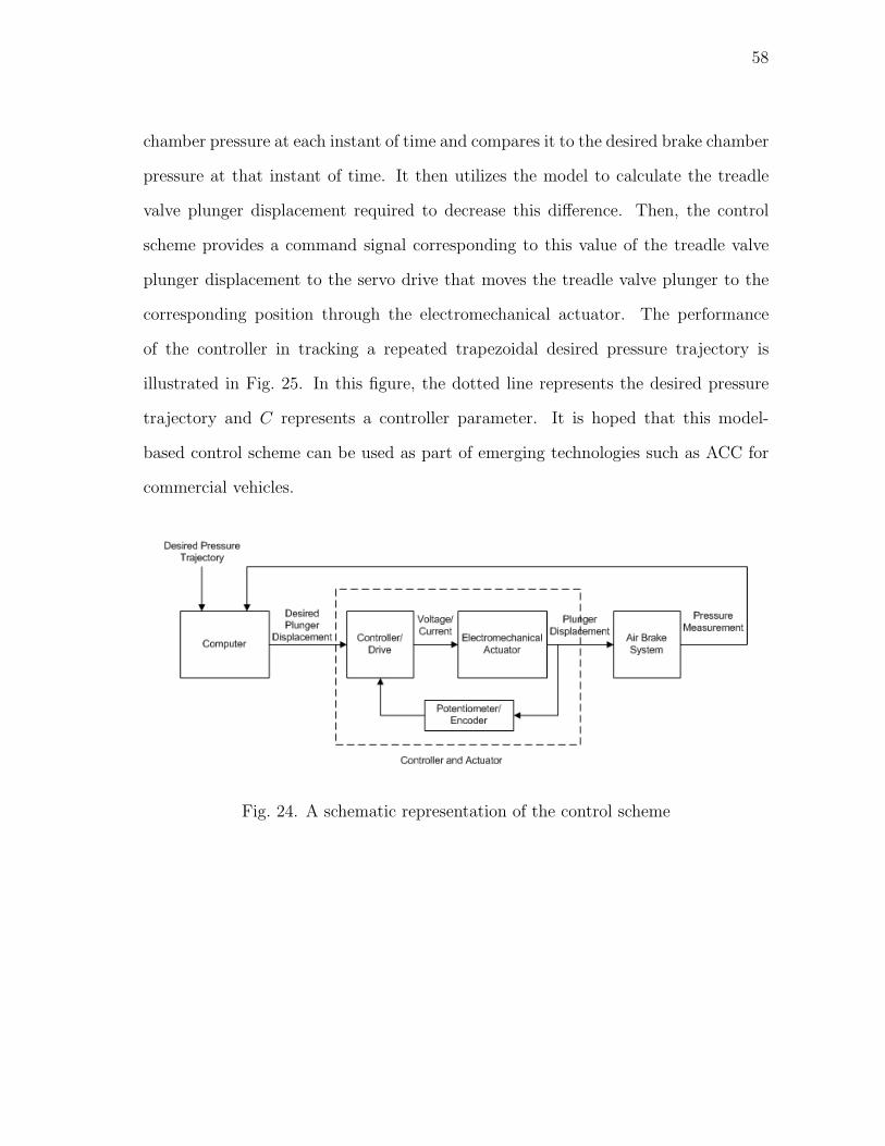
58

chamber pressure at each instant of time and compares it to the desired brake chamber

pressure at that instant of time. It then utilizes the model to calculate the treadle

valve plunger displacement required to decrease this difference. Then, the control

scheme provides a command signal corresponding to this value of the treadle valve

plunger displacement to the servo drive that moves the treadle valve plunger to the

corresponding position through the electromechanical actuator. The performance

of the controller in tracking a repeated trapezoidal desired pressure trajectory is

illustrated in Fig. 25. In this figure, the dotted line represents the desired pressure

trajectory and C represents a controller parameter. It is hoped that this model-

based control scheme can be used as part of emerging technologies such as ACC for

commercial vehicles.

Fig. 24. A schematic representation of the control scheme

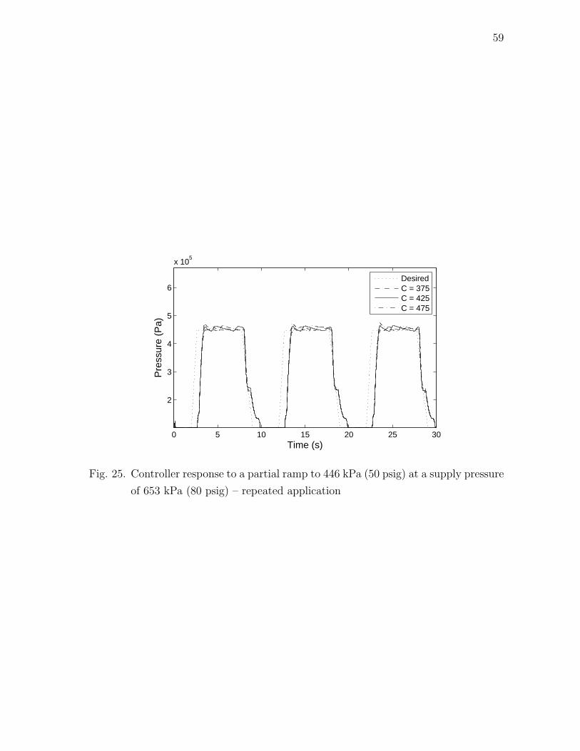
59

0 5 10 15 20 25 30

2

3

4

5

6

x 105

Time (s)

Pre

ssur

e (P

a)

DesiredC = 375C = 425C = 475

Fig. 25. Controller response to a partial ramp to 446 kPa (50 psig) at a supply pressure

of 653 kPa (80 psig) – repeated application

60

CHAPTER V

DETECTION OF LEAKS IN THE AIR BRAKE SYSTEM

In this chapter, a scheme will be presented for monitoring the air brake system for

leaks. In the following chapter, schemes will be presented to estimate the stroke of the

push rod and thus can be used for monitoring the brake system for out-of-adjustment

of push rods. All these schemes will use the model presented in chapter IV and

the measurement of the pressure in the brake chamber. These schemes have been

corroborated with experimental data and the corresponding results will be presented.

Designing a Fault Detection and Isolation (FDI) scheme for a physical system

involves the tasks of residual generation and residual processing. Exhaustive sur-

veys of various FDI schemes have been provided by Willsky [87], Gertler [88], [89],

Basseville [90], Isermann [91] and Frank [92]. Economic constraints require that a re-

liable diagnostic tool be obtained with the least number of sensors. For the proposed

diagnostic system, a pressure transducer is required at each brake chamber and a dis-

placement transducer is required to measure the treadle valve plunger displacement.

The investment on these sensors will be justified by the availability of a fast, reli-

able and automatic diagnostic system. For a given brake application, the governing

equations of the model will be solved numerically to obtain the solution for the brake

chamber pressure. This will be compared with the experimental data to generate the

values of the residuals. The diagnostic schemes will generate the pressure residuals

and process them to detect leaks and estimate the push rod stroke. The features of

the diagnostic schemes proposed in this dissertation include:

1. The presence of a leak will be determined from measurements of the steady

state brake chamber pressure and the supply pressure taken during a full brake

application. The difference between these two values serves as an indicator for

61

the absence or the presence of leaks.

2. The stroke of the push rod will be estimated from the parameter estimation and

transition detection schemes developed using the hybrid model for the pressure

transients in the brake chamber.

Currently in commercial vehicles, leaks can be detected only by manual inspec-

tion. The only available indicator is in the form of a low-pressure warning signal

which is activated when the air pressure in the storage reservoirs falls below around

65 psig 1. But such an indicator will be activated only when the compressor fails

to operate properly and thus is a “worst-case” indicator of leakage. Visual push

rod adjustment indicators are required on all commercial vehicles manufactured from

1994 [11], [12]. But the use of these indicators also involves manual inspection. The

diagnostic schemes presented in this dissertation will use the measurement of the

pressure in the brake chamber along with the model presented in chapter IV to au-

tomatically monitor the brake system for leaks and out-of-adjustment of push rods.

Before presenting the scheme for detecting leaks in the air brake system, a brief re-

view of diagnostic tools that are currently available for monitoring air brake systems

is presented.

A. A brief review of existing diagnostic tools for air brake systems

In this section some of the tools that are currently available to monitor the perfor-

mance of the air brake system are listed. A few patents that have been awarded with

respect to developing diagnostic tools for the air brake system are also presented.

Some of the current on-board diagnostic tools give a warning when the push rod

stroke exceeds the re-adjustment limit. Transducers measure or infer the push rod

1The normal range of pressure in the storage reservoirs is 100-130 psig.

62

stroke and transmit the signals to a decision module that illuminates a warning light

when the stroke exceeds the point of re-adjustment. Also, stroke indicators can be

mounted on the push rod to facilitate visual inspections. Brake pad wear indicators

are also available to help the inspector to check the level of the brake lining wear.

On August 9, 2002, the Federal Motor Carrier Safety Administration (FMCSA)

established a rule to allow for the inspection of commercial vehicles using Performance

Based Brake Testers (PBBTs) [93]. Flat plate testers and roller dynamometers are

two examples of PBBTs. They measure / infer the brake force generated during a

brake application. A few diagnostic systems for air brakes that are commercially

available are listed in Table VI.

In a flat plate tester, brakes are applied on a vehicle in motion and the brake

forces generated on each axle are measured. In a roller dynamometer, the vehicle is

stationary while the wheels of an axle are being rotated on rollers. During a brake

application, the resistance offered by the wheels to the rotation of the rollers is an

indication of the brake forces generated on that axle.

Next, a list of a few recent patents with regards to diagnostic tools for air brake

systems is presented. A more comprehensive list can be found at the website of the

United States Patent and Trademark Office (USPTO) [94]. This list of patents is as

follows:

1. Patent No. 6,754,568 - Brake response analysis system [June 22, 2004]:

This system measures the service brake application and release times and the

parking brake application time and checks for compliance with the requirements

of FMVSS 121. A data acquisition and recording system is provided to record

the pressure in the brake chamber during brake application and release.

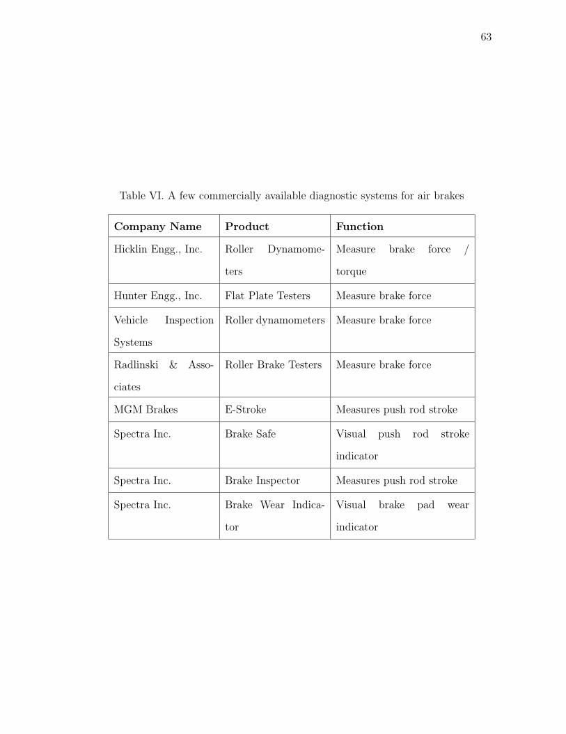
63

Table VI. A few commercially available diagnostic systems for air brakes

Company Name Product Function

Hicklin Engg., Inc. Roller Dynamome-

ters

Measure brake force /

torque

Hunter Engg., Inc. Flat Plate Testers Measure brake force

Vehicle Inspection

Systems

Roller dynamometers Measure brake force

Radlinski & Asso-

ciates

Roller Brake Testers Measure brake force

MGM Brakes E-Stroke Measures push rod stroke

Spectra Inc. Brake Safe Visual push rod stroke

indicator

Spectra Inc. Brake Inspector Measures push rod stroke

Spectra Inc. Brake Wear Indica-

tor

Visual brake pad wear

indicator

64

2. Patent No. 6,215,394 - Air brake stroke adjustment monitoring ap-

paratus and method [April 10, 2001]: This apparatus monitors the stroke of

the push rod by means of an electrical circuit. Two switches are mounted on

the brake chamber and the push rod such that they remain in contact when

the push rod stroke is within acceptable limits. When the stroke crosses the re-

adjustment limit, the contact between the switches is broken and the electrical

circuit becomes open which serves as an indicator of out-of-adjustment of the

push rod.

3. Patent No. 6,019,197 - Air brake stroke gage and seal [February 1,

2000]: It is a visual push rod stroke indicator. An “elastomeric-like” grommet

is mounted on the push rod and acts like a seal to the brake chamber when the

brakes are not applied. A reference rod is mounted parallel to the push rod and

the stroke adjustment is determined by the position of the grommet relative to

this reference rod when the push rod strokes out.

4. Patent No. 5,892,437 - On-board brake warning device for air brake

equipped vehicles [April 6, 1999]: This tool measures certain parameters in

the brake system and compares them with pre-determined values and a fault

is indicated once a pre-determined threshold in the difference is crossed. Some

of the parameters measured include brake line pressure, time lag between pres-

surizing a control brake line from the treadle valve and the application of the

brake, vehicle speed, etc.

5. Patent No. 5,320,198 - Air brake stroke length adjustment gauge [June

14, 1994]: Reference markers are mounted on the clevis of the push rod and

on the arm of the slack adjuster. The state of adjustment of the push rod is

inferred visually by the relative motion of these two indicators when the brake

65

is applied.

Some other patents for monitoring the push rod stroke include Patent No.s 5,358,076,

5,244,061 and 4,879,964.

It can be noted that most of the tools listed above mainly monitor the push rod

stroke. But leakage in the air brake system too affects the performance of the brake

system by increasing the time lag in the brake system and reducing the brake torque

generated. Also, it is possible that the stroke of the push rod is within the prescribed

limits even in the presence of a big leak in the hoses; but the force transmitted to the

drum through the linkages and correspondingly the brake torque will be diminished

due to the leakage. Hence, it is equally important to develop a diagnostic tool that can

detect leaks in the air brake system in addition to estimating the push rod stroke. It

is hoped that the diagnostic schemes presented in this dissertation can be ultimately

incorporated into an on-board / portable diagnostic tool for air brakes that achieves

both of these objectives.

B. A scheme for detecting leaks in air brake systems

In this section, a procedure for detecting leaks in the air brake system from the

measurement of the brake chamber pressure is presented. In the experimental setup, a

leak is introduced in the brake system by loosening the hose couplings at the entrance

of the brake chamber. Brake applications are made at different supply pressures

and the prediction of the model is compared with the corresponding brake chamber

pressure measurement in each case.

During “partial” brake applications (a “partial” application refers to a brake

application where, in the absence of any leaks and other faults, the steady state

brake chamber pressure is less than the supply pressure to the treadle valve) made

66

in the absence of a leak, the inlet port of the primary circuit of the treadle valve will

close at some point during the brake application process (which is determined in the

simulations from the force balance equation, Eq. (4.5)), and there is no further flow of

air in the system until the brakes are applied further or released. It is observed that

at partial brake applications made in the presence of a leak, the brake system tends

to make up for the loss of air due to leakage by continuously bleeding air from the

reservoir until the brakes are released. This effect was observed in the experimental

setup where the air could be heard flowing through the pressure regulator and other

components as long as the brake was kept applied in the presence of a leak. This was

not the case when there were no leaks in the system.

The above observation is illustrated in Fig. 26 where one can hardly notice any

difference between the steady state pressure predicted by the “fault-free” model and

that from the experimental data for a partial brake application test run despite the

presence of a leak in the system. Also, the response of the treadle valve is such that

the full range of brake chamber pressure is realized in a very narrow range of the

plunger displacement. This is illustrated in Figs. 27 and 28 where the steady state

values of the brake chamber pressure and the treadle valve plunger displacement

have been plotted for a wide range of test runs performed at a supply pressure of

653 kPa (80 psig) and 722 kPa (90 psig) respectively. It can be observed that the

majority of the pressure range is achieved within a span of 0.002 m of the plunger

displacement. Thus, the prediction of the steady state brake chamber pressure by

the model at partial applications is sensitive to measurements from the treadle valve

displacement transducer. External factors such as noise, temperature, etc., affect

these measurements and there is invariably some error between the prediction of the

model and the measured steady state brake chamber pressure. This is illustrated

in Figs. 29 and 30 where the steady state brake chamber pressure predicted by the

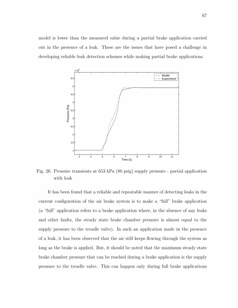
67

model is lower than the measured value during a partial brake application carried

out in the presence of a leak. These are the issues that have posed a challenge in

developing reliable leak detection schemes while making partial brake applications.

3 4 5 6 7 8 9 10 11

1

1.5

2

2.5

3

3.5

4

4.5

5

5.5

x 105

Time (s)

Pre

ssur

e (P

a)

ModelExperiment

Fig. 26. Pressure transients at 653 kPa (80 psig) supply pressure - partial application

with leak

It has been found that a reliable and repeatable manner of detecting leaks in the

current configuration of the air brake system is to make a “full” brake application

(a “full” application refers to a brake application where, in the absence of any leaks

and other faults, the steady state brake chamber pressure is almost equal to the

supply pressure to the treadle valve). In such an application made in the presence

of a leak, it has been observed that the air still keeps flowing through the system as

long as the brake is applied. But, it should be noted that the maximum steady state

brake chamber pressure that can be reached during a brake application is the supply

pressure to the treadle valve. This can happen only during full brake applications

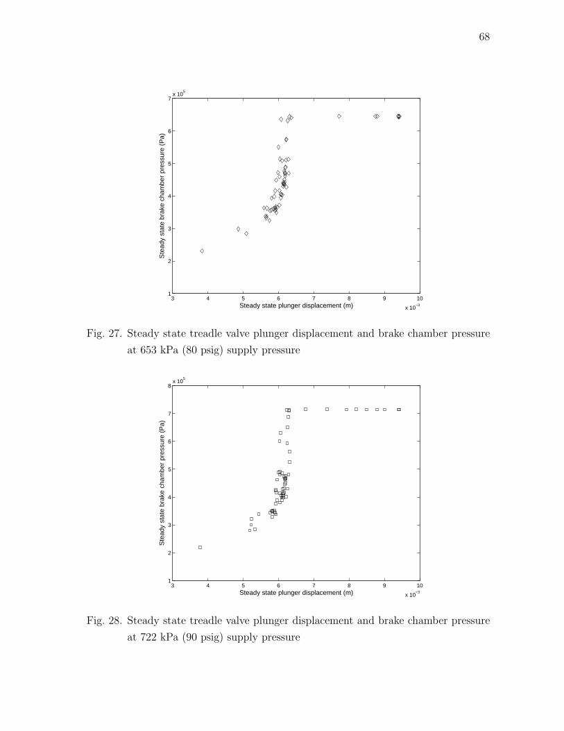
68

3 4 5 6 7 8 9 10

x 10−3

1

2

3

4

5

6

7x 10

5

Steady state plunger displacement (m)

Ste

ady

stat

e br

ake

cham

ber

pres

sure

(P

a)

Fig. 27. Steady state treadle valve plunger displacement and brake chamber pressure

at 653 kPa (80 psig) supply pressure

3 4 5 6 7 8 9 10

x 10−3

1

2

3

4

5

6

7

8x 10

5

Steady state plunger displacement (m)

Ste

ady

stat

e br

ake

cham

ber

pres

sure

(P

a)

Fig. 28. Steady state treadle valve plunger displacement and brake chamber pressure


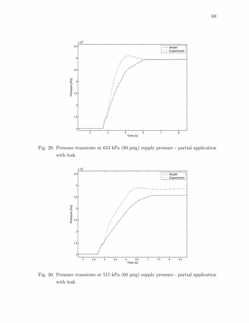
69

3 4 5 6 7 8

1

1.5

2

2.5

3

3.5

4

4.5

x 105

Time (s)

Pre

ssur

e (P

a)

ModelExperiment


with leak

4 4.5 5 5.5 6 6.5 7 7.5 8 8.5

1

1.5

2

2.5

3

3.5

4

4.5

x 105

Time (s)

Pre

ssur

e (P

a)

ModelExperiment


with leak

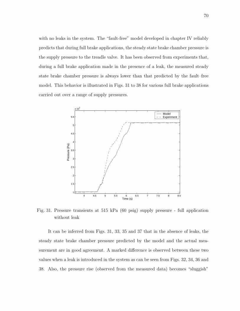
70

with no leaks in the system. The “fault-free” model developed in chapter IV reliably

predicts that during full brake applications, the steady state brake chamber pressure is

the supply pressure to the treadle valve. It has been observed from experiments that,

during a full brake application made in the presence of a leak, the measured steady

state brake chamber pressure is always lower than that predicted by the fault–free

model. This behavior is illustrated in Figs. 31 to 38 for various full brake applications

carried out over a range of supply pressures.

4 4.5 5 5.5 6 6.5 7 7.5 8 8.5

1

1.5

2

2.5

3

3.5

4

4.5

5

5.5

x 105

Time (s)

Pre

ssur

e (P

a)

ModelExperiment

Fig. 31. Pressure transients at 515 kPa (60 psig) supply pressure - full application

without leak

It can be inferred from Figs. 31, 33, 35 and 37 that in the absence of leaks, the

steady state brake chamber pressure predicted by the model and the actual mea-

surement are in good agreement. A marked difference is observed between these two

values when a leak is introduced in the system as can be seen from Figs. 32, 34, 36 and

38. Also, the pressure rise (observed from the measured data) becomes “sluggish”

71

3.5 4 4.5 5 5.5 6 6.5 7 7.5 8

1

1.5

2

2.5

3

3.5

4

4.5

5

5.5

6

x 105

Time (s)

Pre

ssur

e (P

a)

ModelExperiment

Fig. 32. Pressure transients at 515 kPa (60 psig) supply pressure - full application with

leak

3.5 4 4.5 5 5.5 6 6.5 7 7.5 8

1

2

3

4

5

6

x 105

Time (s)

Pre

ssur

e (P

a)

ModelExperiment


without leak

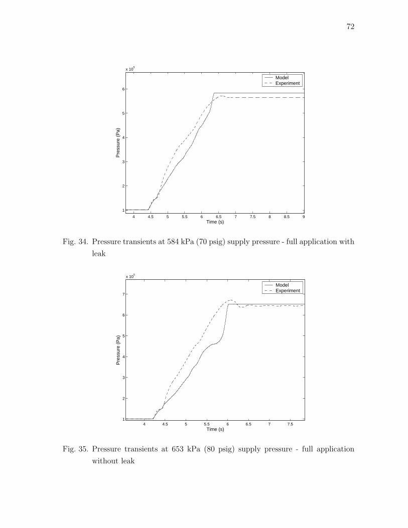
72

4 4.5 5 5.5 6 6.5 7 7.5 8 8.5 9

1

2

3

4

5

6

x 105

Time (s)

Pre

ssur

e (P

a)

ModelExperiment


leak

4 4.5 5 5.5 6 6.5 7 7.51

2

3

4

5

6

7

x 105

Time (s)

Pre

ssur

e (P

a)

ModelExperiment


without leak

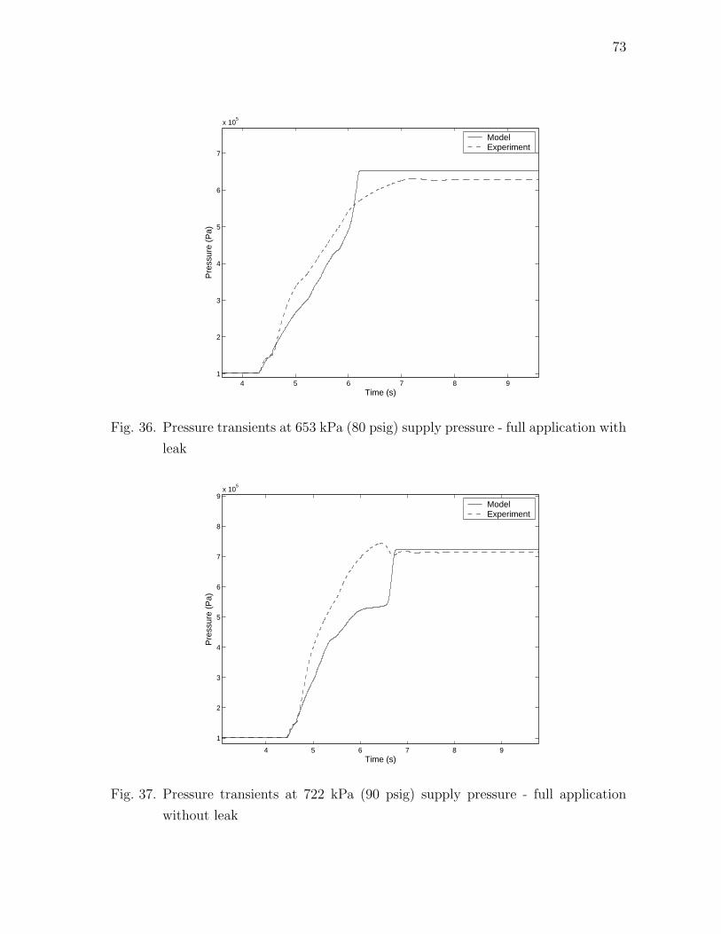
73

4 5 6 7 8 91

2

3

4

5

6

7

x 105

Time (s)

Pre

ssur

e (P

a)

ModelExperiment


leak

4 5 6 7 8 9

1

2

3

4

5

6

7

8

9x 10

5

Time (s)

Pre

ssur

e (P

a)

ModelExperiment


without leak

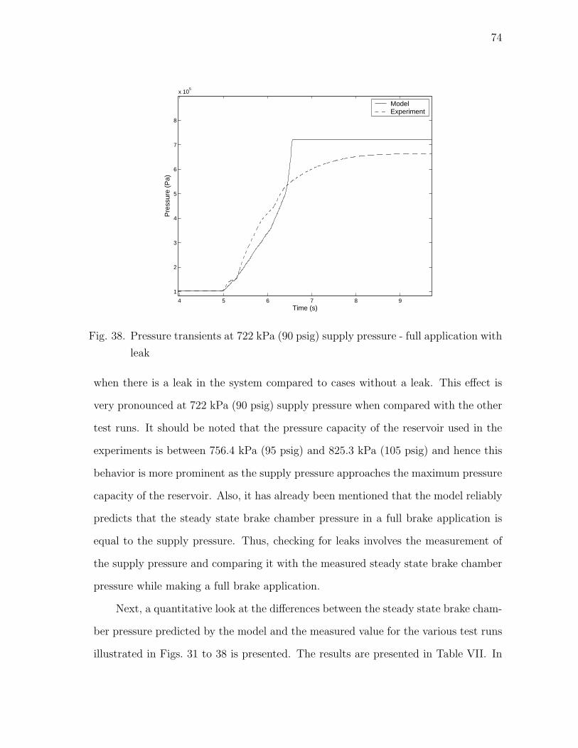
74

4 5 6 7 8 9

1

2

3

4

5

6

7

8

x 105

Time (s)

Pre

ssur

e (P

a)

ModelExperiment


leak

when there is a leak in the system compared to cases without a leak. This effect is

very pronounced at 722 kPa (90 psig) supply pressure when compared with the other

test runs. It should be noted that the pressure capacity of the reservoir used in the

experiments is between 756.4 kPa (95 psig) and 825.3 kPa (105 psig) and hence this

behavior is more prominent as the supply pressure approaches the maximum pressure

capacity of the reservoir. Also, it has already been mentioned that the model reliably

predicts that the steady state brake chamber pressure in a full brake application is

equal to the supply pressure. Thus, checking for leaks involves the measurement of

the supply pressure and comparing it with the measured steady state brake chamber

pressure while making a full brake application.

Next, a quantitative look at the differences between the steady state brake cham-

ber pressure predicted by the model and the measured value for the various test runs

illustrated in Figs. 31 to 38 is presented. The results are presented in Table VII. In

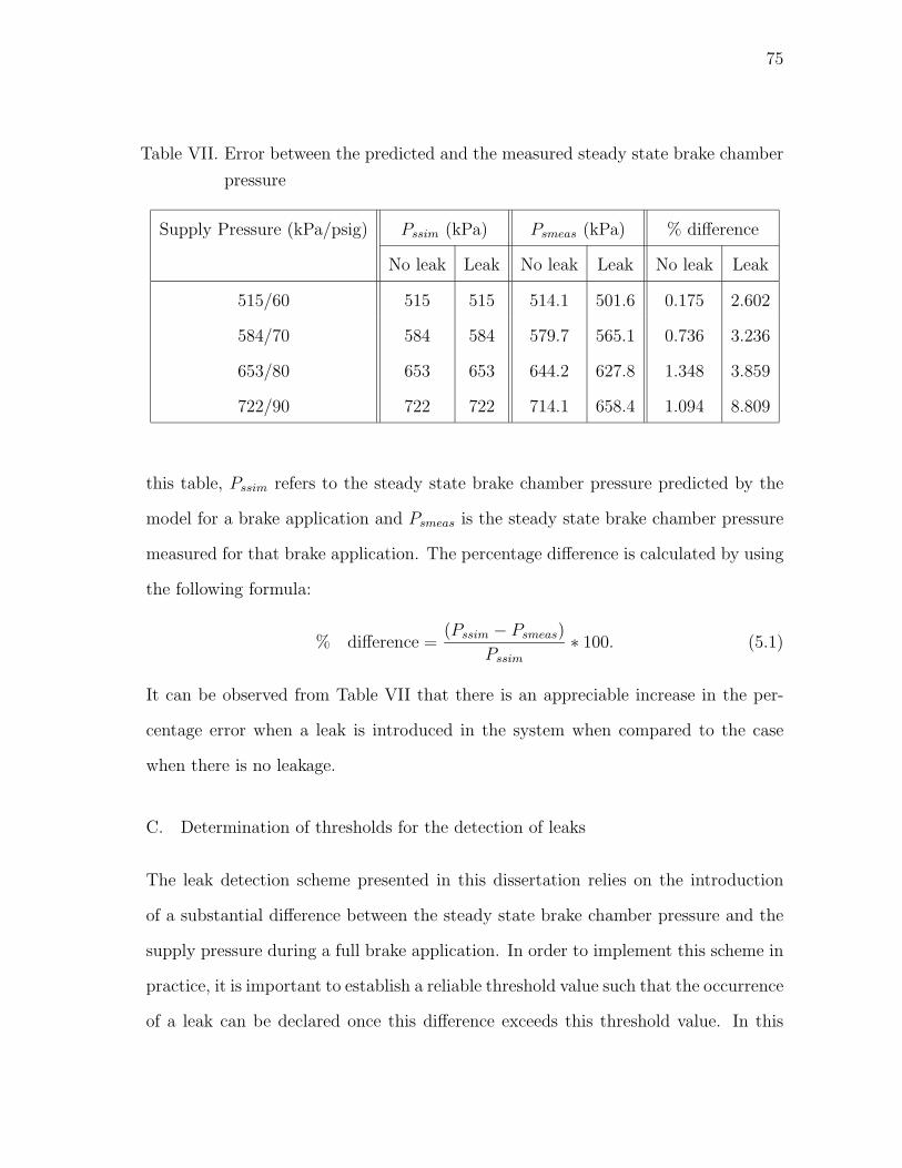
75

Table VII. Error between the predicted and the measured steady state brake chamber

pressure

Supply Pressure (kPa/psig) Pssim (kPa) Psmeas (kPa) % difference

No leak Leak No leak Leak No leak Leak

515/60 515 515 514.1 501.6 0.175 2.602

584/70 584 584 579.7 565.1 0.736 3.236

653/80 653 653 644.2 627.8 1.348 3.859

722/90 722 722 714.1 658.4 1.094 8.809

this table, Pssim refers to the steady state brake chamber pressure predicted by the

model for a brake application and Psmeas is the steady state brake chamber pressure

measured for that brake application. The percentage difference is calculated by using

the following formula:

% difference =(Pssim − Psmeas)

Pssim

∗ 100. (5.1)

It can be observed from Table VII that there is an appreciable increase in the per-

centage error when a leak is introduced in the system when compared to the case

when there is no leakage.

C. Determination of thresholds for the detection of leaks

The leak detection scheme presented in this dissertation relies on the introduction

of a substantial difference between the steady state brake chamber pressure and the

supply pressure during a full brake application. In order to implement this scheme in

practice, it is important to establish a reliable threshold value such that the occurrence

of a leak can be declared once this difference exceeds this threshold value. In this

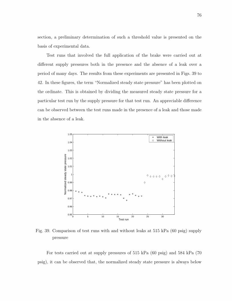
76

section, a preliminary determination of such a threshold value is presented on the

basis of experimental data.

Test runs that involved the full application of the brake were carried out at

different supply pressures both in the presence and the absence of a leak over a

period of many days. The results from these experiments are presented in Figs. 39 to

42. In these figures, the term “Normalized steady state pressure” has been plotted on

the ordinate. This is obtained by dividing the measured steady state pressure for a

particular test run by the supply pressure for that test run. An appreciable difference

can be observed between the test runs made in the presence of a leak and those made

in the absence of a leak.

0 5 10 15 20 25 300.95

0.96

0.97

0.98

0.99

1

1.01

1.02

1.03

1.04

1.05

Test run

Nor

mal

ized

ste

ady

stat

e pr

essu

re

With leakWithout leak

Fig. 39. Comparison of test runs with and without leaks at 515 kPa (60 psig) supply

pressure

For tests carried out at supply pressures of 515 kPa (60 psig) and 584 kPa (70

psig), it can be observed that, the normalized steady state pressure is always below

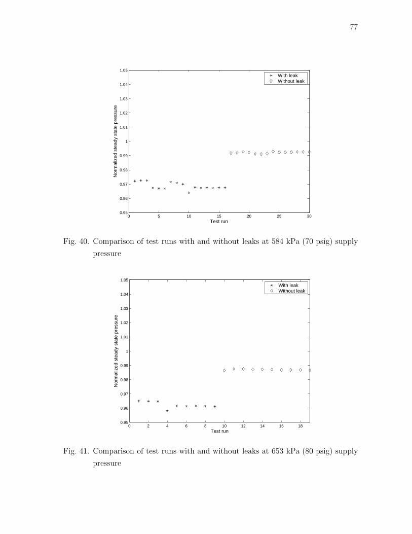
77

0 5 10 15 20 25 300.95

0.96

0.97

0.98

0.99

1

1.01

1.02

1.03

1.04

1.05

Test run

Nor

mal

ized

ste

ady

stat

e pr

essu

re



pressure

0 2 4 6 8 10 12 14 16 180.95

0.96

0.97

0.98

0.99

1

1.01

1.02

1.03

1.04

1.05

Test run

Nor

mal

ized

ste

ady

stat

e pr

essu

re



pressure

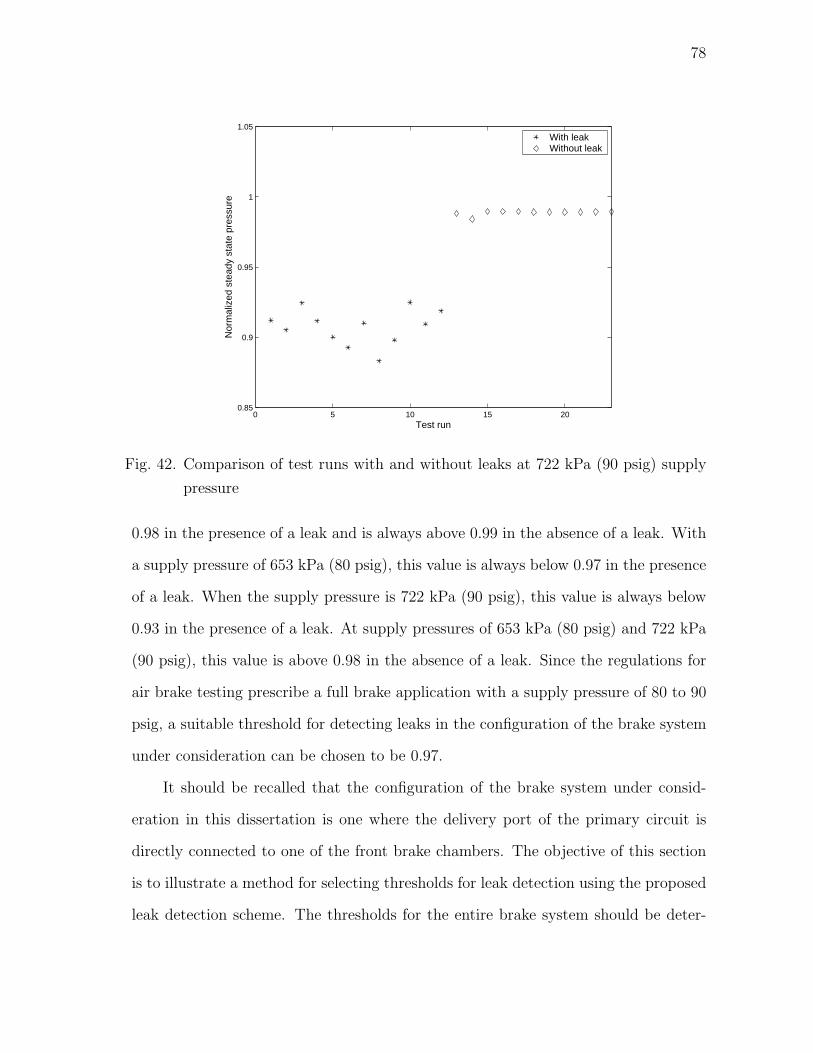
78

0 5 10 15 200.85

0.9

0.95

1

1.05

Test run

Nor

mal

ized

ste

ady

stat

e pr

essu

re



pressure

0.98 in the presence of a leak and is always above 0.99 in the absence of a leak. With

a supply pressure of 653 kPa (80 psig), this value is always below 0.97 in the presence

of a leak. When the supply pressure is 722 kPa (90 psig), this value is always below

0.93 in the presence of a leak. At supply pressures of 653 kPa (80 psig) and 722 kPa

(90 psig), this value is above 0.98 in the absence of a leak. Since the regulations for

air brake testing prescribe a full brake application with a supply pressure of 80 to 90

psig, a suitable threshold for detecting leaks in the configuration of the brake system

under consideration can be chosen to be 0.97.

It should be recalled that the configuration of the brake system under consid-

eration in this dissertation is one where the delivery port of the primary circuit is

directly connected to one of the front brake chambers. The objective of this section

is to illustrate a method for selecting thresholds for leak detection using the proposed

leak detection scheme. The thresholds for the entire brake system should be deter-

79

mined by carrying out experiments on the air brake system in an actual commercial

vehicle. Many factors affect the selection of these threshold values. The accuracy of

the pressure sensor plays a vital role in the determination of thresholds. Also, the air

brake system contains check valves that will operate only when the difference between

the pressure at the inlet port and the outlet port exceeds a certain minimum value

(usually 2 to 3 psig). Due to the presence of such valves, the steady state pressure in

the brake chamber might be less than the supply pressure even in the absence of a

leak. Thus, the presence of such valves may also affect the selection of thresholds for

leak detection.

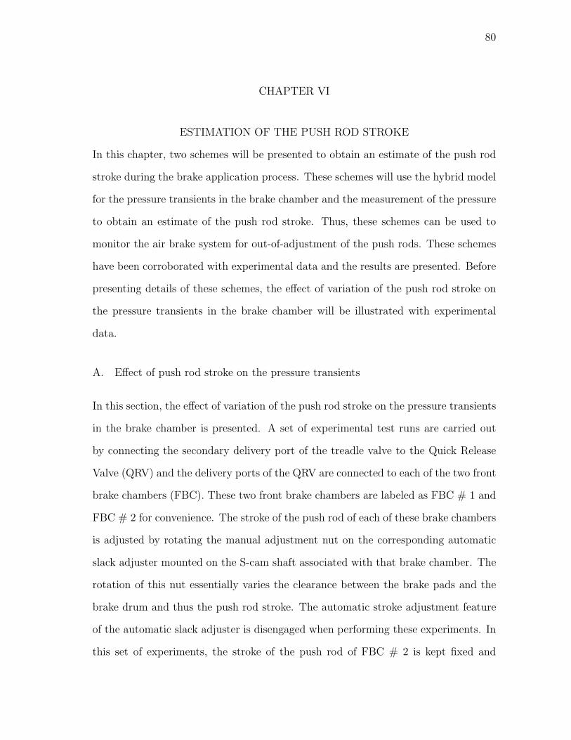
80

CHAPTER VI

ESTIMATION OF THE PUSH ROD STROKE

In this chapter, two schemes will be presented to obtain an estimate of the push rod

stroke during the brake application process. These schemes will use the hybrid model

for the pressure transients in the brake chamber and the measurement of the pressure

to obtain an estimate of the push rod stroke. Thus, these schemes can be used to

monitor the air brake system for out-of-adjustment of the push rods. These schemes

have been corroborated with experimental data and the results are presented. Before

presenting details of these schemes, the effect of variation of the push rod stroke on

the pressure transients in the brake chamber will be illustrated with experimental

data.

A. Effect of push rod stroke on the pressure transients

In this section, the effect of variation of the push rod stroke on the pressure transients

in the brake chamber is presented. A set of experimental test runs are carried out

by connecting the secondary delivery port of the treadle valve to the Quick Release

Valve (QRV) and the delivery ports of the QRV are connected to each of the two front

brake chambers (FBC). These two front brake chambers are labeled as FBC # 1 and

FBC # 2 for convenience. The stroke of the push rod of each of these brake chambers

is adjusted by rotating the manual adjustment nut on the corresponding automatic

slack adjuster mounted on the S-cam shaft associated with that brake chamber. The

rotation of this nut essentially varies the clearance between the brake pads and the

brake drum and thus the push rod stroke. The automatic stroke adjustment feature

of the automatic slack adjuster is disengaged when performing these experiments. In

this set of experiments, the stroke of the push rod of FBC # 2 is kept fixed and

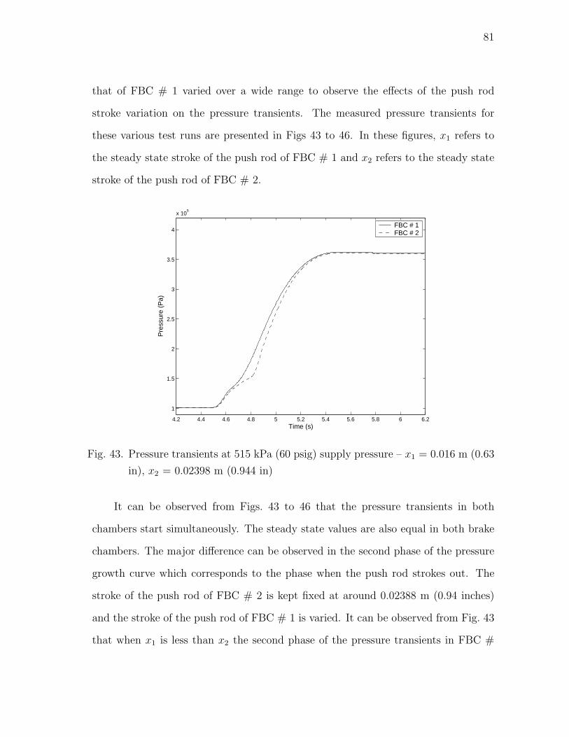
81

that of FBC # 1 varied over a wide range to observe the effects of the push rod

stroke variation on the pressure transients. The measured pressure transients for

these various test runs are presented in Figs 43 to 46. In these figures, x1 refers to

the steady state stroke of the push rod of FBC # 1 and x2 refers to the steady state

stroke of the push rod of FBC # 2.

4.2 4.4 4.6 4.8 5 5.2 5.4 5.6 5.8 6 6.2

1

1.5

2

2.5

3

3.5

4

x 105

Time (s)

Pre

ssur

e (P

a)

FBC # 1FBC # 2

Fig. 43. Pressure transients at 515 kPa (60 psig) supply pressure – x1 = 0.016 m (0.63

in), x2 = 0.02398 m (0.944 in)

It can be observed from Figs. 43 to 46 that the pressure transients in both

chambers start simultaneously. The steady state values are also equal in both brake

chambers. The major difference can be observed in the second phase of the pressure

growth curve which corresponds to the phase when the push rod strokes out. The

stroke of the push rod of FBC # 2 is kept fixed at around 0.02388 m (0.94 inches)

and the stroke of the push rod of FBC # 1 is varied. It can be observed from Fig. 43

that when x1 is less than x2 the second phase of the pressure transients in FBC #

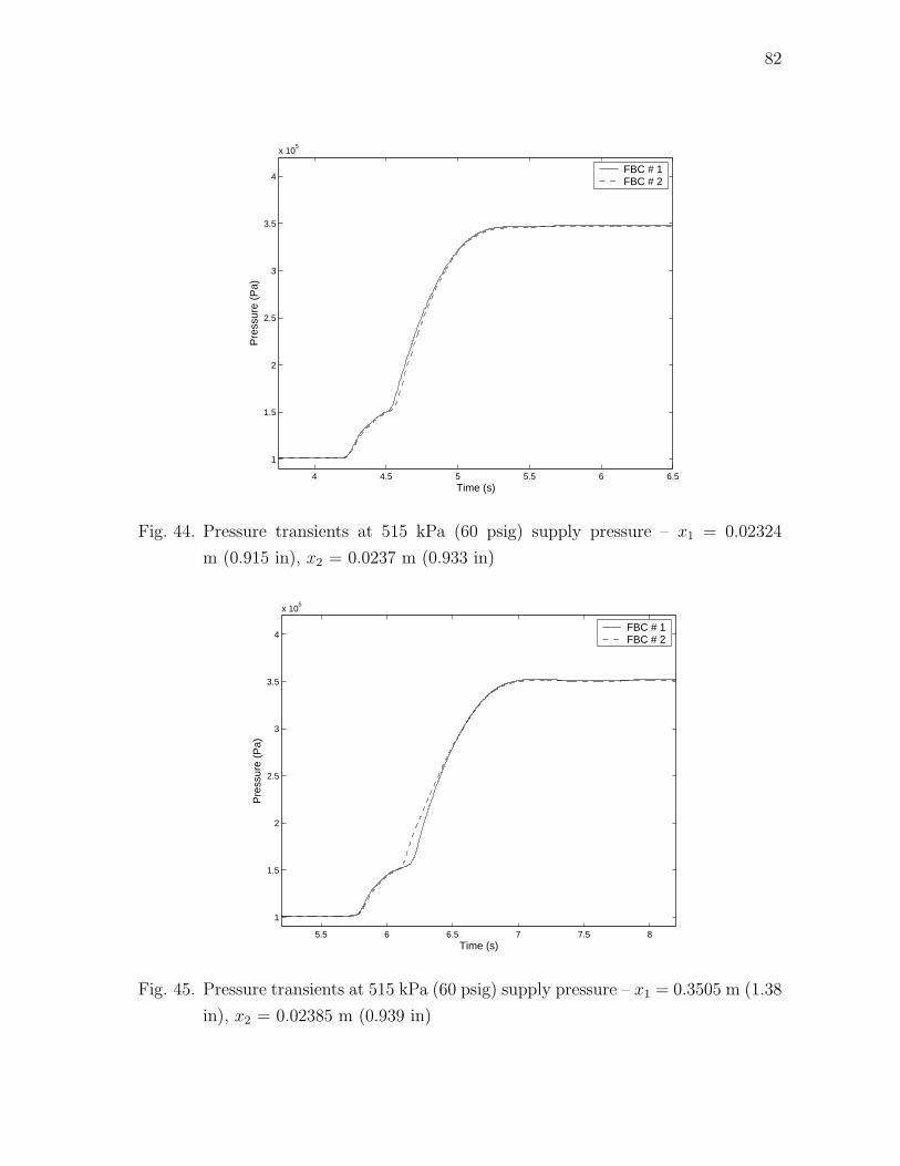
82

4 4.5 5 5.5 6 6.5

1

1.5

2

2.5

3

3.5

4

x 105

Time (s)

Pre

ssur

e (P

a)

FBC # 1FBC # 2

Fig. 44. Pressure transients at 515 kPa (60 psig) supply pressure – x1 = 0.02324

m (0.915 in), x2 = 0.0237 m (0.933 in)

5.5 6 6.5 7 7.5 8

1

1.5

2

2.5

3

3.5

4

x 105

Time (s)

Pre

ssur

e (P

a)

FBC # 1FBC # 2

Fig. 45. Pressure transients at 515 kPa (60 psig) supply pressure – x1 = 0.3505 m (1.38

in), x2 = 0.02385 m (0.939 in)

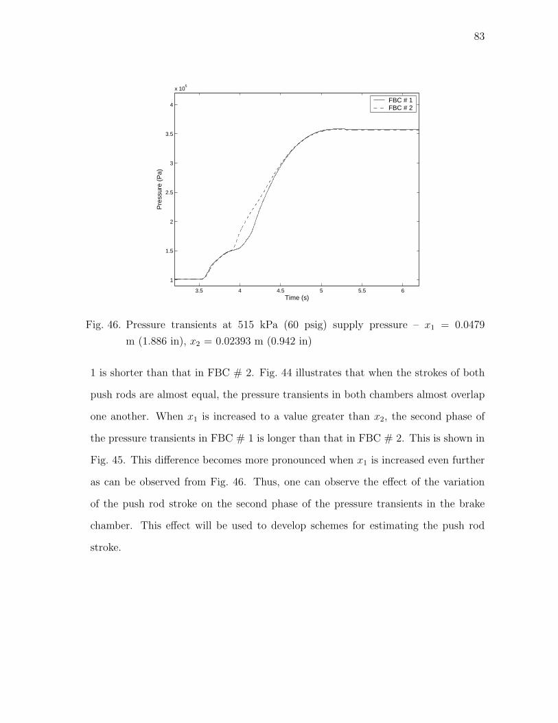
83

3.5 4 4.5 5 5.5 6

1

1.5

2

2.5

3

3.5

4

x 105

Time (s)

Pre

ssur

e (P

a)

FBC # 1FBC # 2

Fig. 46. Pressure transients at 515 kPa (60 psig) supply pressure – x1 = 0.0479

m (1.886 in), x2 = 0.02393 m (0.942 in)

1 is shorter than that in FBC # 2. Fig. 44 illustrates that when the strokes of both

push rods are almost equal, the pressure transients in both chambers almost overlap

one another. When x1 is increased to a value greater than x2, the second phase of

the pressure transients in FBC # 1 is longer than that in FBC # 2. This is shown in

Fig. 45. This difference becomes more pronounced when x1 is increased even further

as can be observed from Fig. 46. Thus, one can observe the effect of the variation

of the push rod stroke on the second phase of the pressure transients in the brake

chamber. This effect will be used to develop schemes for estimating the push rod

stroke.

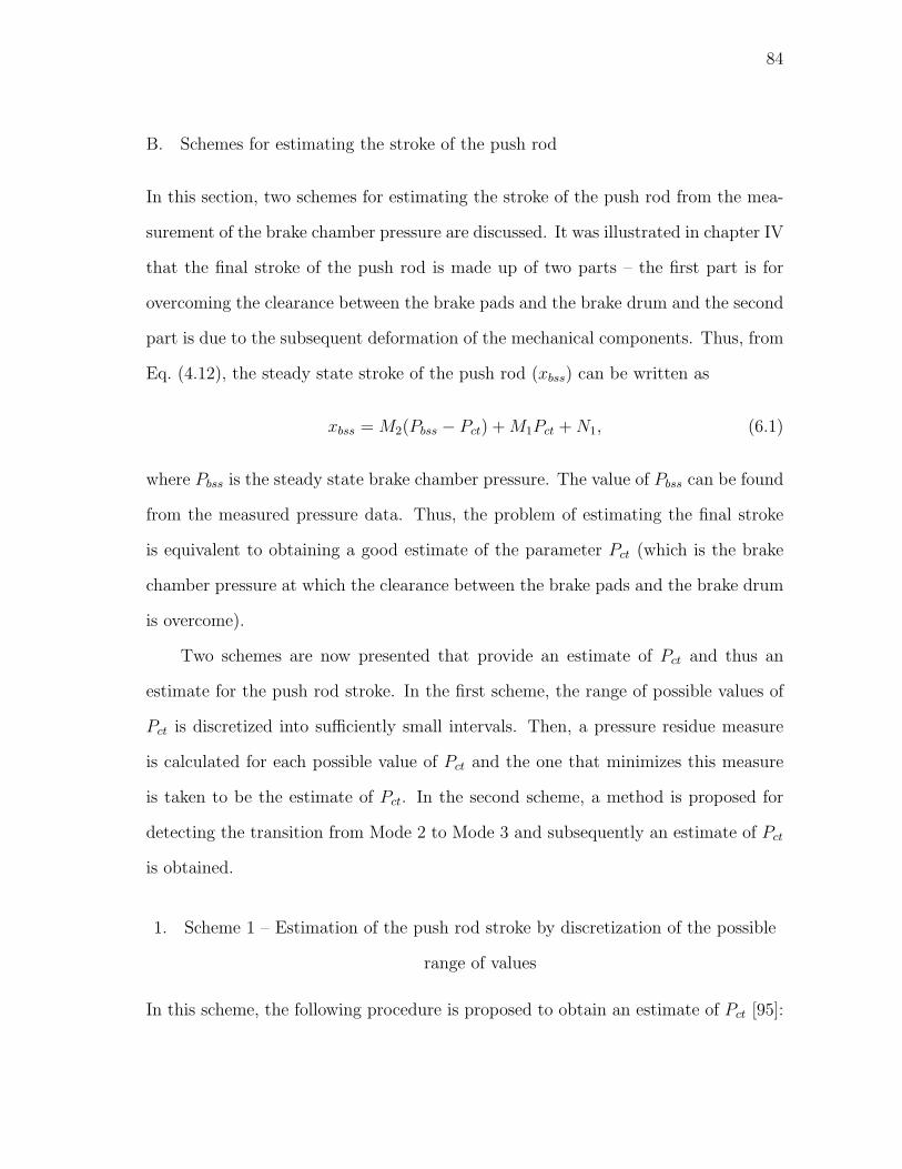
84

B. Schemes for estimating the stroke of the push rod

In this section, two schemes for estimating the stroke of the push rod from the mea-

surement of the brake chamber pressure are discussed. It was illustrated in chapter IV

that the final stroke of the push rod is made up of two parts – the first part is for

overcoming the clearance between the brake pads and the brake drum and the second

part is due to the subsequent deformation of the mechanical components. Thus, from

Eq. (4.12), the steady state stroke of the push rod (xbss) can be written as

xbss = M2(Pbss − Pct) + M1Pct + N1, (6.1)

where Pbss is the steady state brake chamber pressure. The value of Pbss can be found

from the measured pressure data. Thus, the problem of estimating the final stroke

is equivalent to obtaining a good estimate of the parameter Pct (which is the brake

chamber pressure at which the clearance between the brake pads and the brake drum

is overcome).

Two schemes are now presented that provide an estimate of Pct and thus an

estimate for the push rod stroke. In the first scheme, the range of possible values of

Pct is discretized into sufficiently small intervals. Then, a pressure residue measure

is calculated for each possible value of Pct and the one that minimizes this measure

is taken to be the estimate of Pct. In the second scheme, a method is proposed for

detecting the transition from Mode 2 to Mode 3 and subsequently an estimate of Pct

is obtained.

1. Scheme 1 – Estimation of the push rod stroke by discretization of the possible

range of values

In this scheme, the following procedure is proposed to obtain an estimate of Pct [95]:

85

1. From the physical limits on the stroke of the push rod, bounds on the value of

Pct can be obtained. Let Pctl and Pctu denote respectively the lower bound and

the upper bound on Pct. It should be noted that the lower bound corresponds

to zero clearance between the brake pad and the brake drum and the upper

bound is obtained from the maximum possible push rod stroke. The maximum

push rod stroke for the “Type-20” brake chamber that is being used in the

experimental setup is 0.05715 m (2.25 in) [96]. The value of Pctl is found from

experiments to be 142.73 kPa (6 psig) and the value of Pctu is calculated to be

184.1 kPa (12 psig).

2. The estimate of Pct, denoted by Pct, will lie in the interval between Pctl and

Pctu. In order to obtain this value, the interval [Pctl, Pctu] is discretized into

finer intervals by using a step size (δP ) of 689.5 Pa (0.1 psi). Thus, a set

P is obtained whose elements are equally spaced by a step size of δP and

whose first and last elements are Pctl and Pctu respectively. It was illustrated in

chapter IV that, the push rod stroke needed to overcome the clearance between

the brake pads and the brake drum is reflected in the second region (Mode 2)

of the pressure growth curve. Hence, the focus is restricted to this region for

obtaining Pct.

3. Next, the governing equations of the model (Eqs. (4.5), (4.14) and (4.15)) are

solved numerically for each element in the set P to obtain the corresponding

solution of the brake chamber pressure. Then, the following pressure error /

residue measure is calculated:

eP (Pcti) =k∑

j=0

|Pmeas(j) − Pb(Pcti)(j)|, (6.2)

where Pmeas(j) is the measured brake chamber pressure at the jth instant of

86

time and Pb(Pcti)(j) is the solution of the model (at the same instant of time)

corresponding to Pcti which is given by

Pcti = Pctl + (δP )i, i = 0, . . . , N, (6.3)

where δP =(Pcti − Pctl)

N.

4. The choice of k in Eq. (6.2) is determined by the maximum possible dwell time

of the system in Mode 2. Depending on the brake pad to brake drum clearance

this time interval will vary. But it has been observed from experiments that

this time interval is usually not more than 0.3–0.35 seconds. The sampling

time used in the experiments is 2 milliseconds. Hence, the value of k is chosen

to be 200 (which corresponds to a time interval of 0.4 seconds). It should

be pointed out that j = 0 corresponds to the time instant at which Mode 2

starts. Hence, one starts at the beginning of Mode 2 (which occurs when the

brake chamber pressure reaches the threshold pressure (Pth)) and calculates the

quantity eP (Pcti) given by Eq. (6.2). This procedure is repeated for each value

of Pcti and finally an array of values representing the residue measure given by

Eq. (6.2) is generated. Then, the estimate Pct is obtained as

Pct = argminPcti∈PeP (Pcti). (6.4)

The results obtained by using this scheme on two test runs are illustrated in

Fig. 47 and Fig. 48. Before discussing the results a few practical issues involved in

implementing the scheme are pointed out. Obtaining accurate measurements of the

brake chamber pressure and the treadle valve plunger displacement is critical to the

successful implementation of this scheme. In reality, measurements are corrupted by

noise and environmental factors. Efforts have been made to minimize the effects of

87

noise by using shielded twisted pair cables for transmitting electrical signals. Also, a

shielded connector block has been used for interfacing the transducers with the DAQ

board. Environmental effects such as temperature, humidity, etc., try to shift the

initial reading (“zero reading”) of the transducers and also affect their calibration

curves. These effects are minimized by obtaining the initial readings at the start

of each and every set of experiments and taking their variation into account while

converting voltage signals into physical quantities (such as pressure, displacement,

etc.). Also, a digital filter with a cut-off frequency of 10 Hz. is used to further

minimize the effect of noise.

In Fig. 47, the results obtained for a test run made at 653 kPa (80 psig) supply

pressure are plotted. The array of the pressure error / residue is calculated and the

minimum value is located and the estimate Pct is obtained from P as the value corre-

sponding to this minimum residue. On the ordinate the term “Normalized pressure

residue” has been plotted. The values corresponding to this term are obtained by

dividing the array of the residues by its minimum value (thus the minimum residue

will always be given a value of 1). Once the value of Pct is determined an estimate

of the final push rod stroke is obtained by using Eq. (6.1). In this case, the best

estimate of the push rod stroke is obtained to be 0.03381 m (1.3311 in) while the

measured value of the stroke is 0.03114 m (1.2262 in). It can be observed that the

normalized pressure residue corresponding to the actual stroke is around 1.007 which

differs by 0.7 % from the residue corresponding to the estimated stroke. In Fig. 48,

the results obtained from a test run performed at a supply pressure of 722 kPa (90

psig) on a different day from the above test run are presented. It is observed that the

estimated push rod stroke in this case is 0.03684 m (1.4506 in) while the measured

stroke is 0.03181 m (1.2525 in). It can be noted that the normalized pressure residue

corresponding to the actual stroke is around 1.009, i.e., a difference of 0.9 % from the

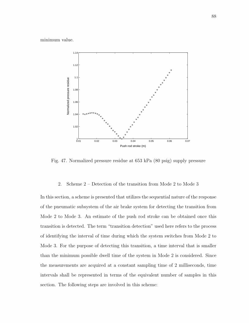
88

minimum value.

0.01 0.02 0.03 0.04 0.05 0.06 0.071

1.02

1.04

1.06

1.08

1.1

1.12

1.14

Push rod stroke (m)

Nor

mal

ized

pre

ssur

e re

sidu

e

Fig. 47. Normalized pressure residue at 653 kPa (80 psig) supply pressure

2. Scheme 2 – Detection of the transition from Mode 2 to Mode 3

In this section, a scheme is presented that utilizes the sequential nature of the response

of the pneumatic subsystem of the air brake system for detecting the transition from

Mode 2 to Mode 3. An estimate of the push rod stroke can be obtained once this

transition is detected. The term “transition detection” used here refers to the process

of identifying the interval of time during which the system switches from Mode 2 to

Mode 3. For the purpose of detecting this transition, a time interval that is smaller

than the minimum possible dwell time of the system in Mode 2 is considered. Since

the measurements are acquired at a constant sampling time of 2 milliseconds, time

intervals shall be represented in terms of the equivalent number of samples in this

section. The following steps are involved in this scheme:

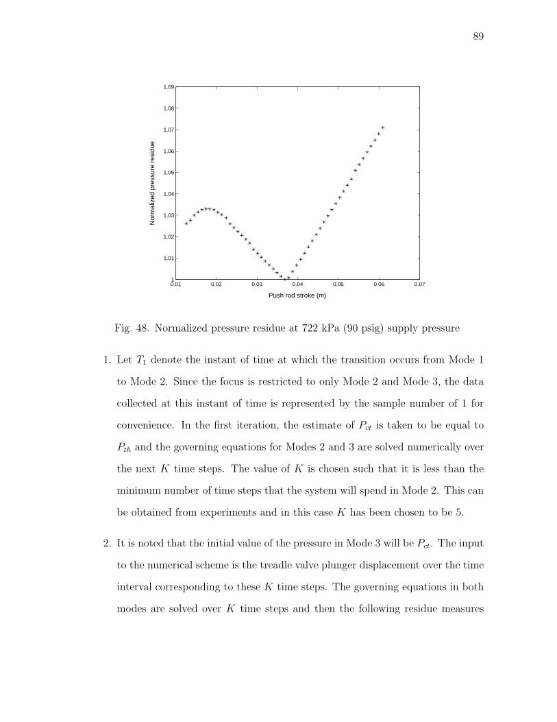
89

0.01 0.02 0.03 0.04 0.05 0.06 0.071

1.01

1.02

1.03

1.04

1.05

1.06

1.07

1.08

1.09

Push rod stroke (m)

Nor

mal

ized

pre

ssur

e re

sidu

e

Fig. 48. Normalized pressure residue at 722 kPa (90 psig) supply pressure

1. Let T1 denote the instant of time at which the transition occurs from Mode 1

to Mode 2. Since the focus is restricted to only Mode 2 and Mode 3, the data

collected at this instant of time is represented by the sample number of 1 for

convenience. In the first iteration, the estimate of Pct is taken to be equal to

Pth and the governing equations for Modes 2 and 3 are solved numerically over

the next K time steps. The value of K is chosen such that it is less than the

minimum number of time steps that the system will spend in Mode 2. This can

be obtained from experiments and in this case K has been chosen to be 5.

2. It is noted that the initial value of the pressure in Mode 3 will be Pct. The input

to the numerical scheme is the treadle valve plunger displacement over the time

interval corresponding to these K time steps. The governing equations in both

modes are solved over K time steps and then the following residue measures

90

are calculated:

e2 =K∑

j=1

|Pmeas(j) − Pb2(j)|, (6.5)

e3 =K∑

j=1

|Pmeas(j) − Pb3(j)|, (6.6)

where Pb2(j) and Pb3(j) are the solutions of the governing equations in Mode 2

and Mode 3 respectively.

3. If e2 < e3, it can be concluded that the system is still in Mode 2. The value of

Pct is updated to be equal to Pb2(K) and the previous step is repeated over the

next K time steps.

4. If e2 ≥ e3, it can be declared that a transition has taken place from Mode 2 to

Mode 3. Then, the best estimate of Pct will be the value used at the start of

this particular iteration. Once this is known, an estimate of the push rod stroke

can be obtained from Eq. (6.1).

In Figs. 49 and 50, the results of this scheme are illustrated on the two test runs

that have been considered in section 1. The initial time interval is taken to be that

corresponding to 50 time steps. This was picked on practical considerations since it

is known that the clearance between the brake pads and the brake drum is never zero

and usually a minimum stroke of around 0.0127 m (0.5 in) is needed to overcome

this clearance. Such a choice also ensures that any initial disagreement between the

model and the experiment at the end of Mode 1 will not affect the transition detection

process. Additionally, it reduces the computation time involved.

In Table VIII, a comparison of the push rod stroke estimate obtained from these

two schemes with the measured stroke is presented. It should be pointed out that

the computation time involved in implementing Scheme 2 is much less than that of

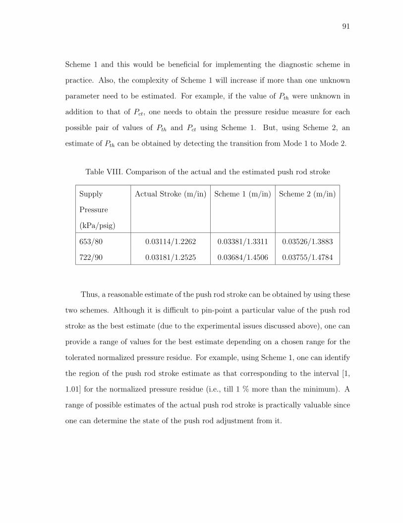
91

Scheme 1 and this would be beneficial for implementing the diagnostic scheme in

practice. Also, the complexity of Scheme 1 will increase if more than one unknown

parameter need to be estimated. For example, if the value of Pth were unknown in

addition to that of Pct, one needs to obtain the pressure residue measure for each

possible pair of values of Pth and Pct using Scheme 1. But, using Scheme 2, an

estimate of Pth can be obtained by detecting the transition from Mode 1 to Mode 2.

Table VIII. Comparison of the actual and the estimated push rod stroke

Supply

Pressure

(kPa/psig)

Actual Stroke (m/in) Scheme 1 (m/in) Scheme 2 (m/in)

653/80 0.03114/1.2262 0.03381/1.3311 0.03526/1.3883

722/90 0.03181/1.2525 0.03684/1.4506 0.03755/1.4784

Thus, a reasonable estimate of the push rod stroke can be obtained by using these

two schemes. Although it is difficult to pin-point a particular value of the push rod

stroke as the best estimate (due to the experimental issues discussed above), one can

provide a range of values for the best estimate depending on a chosen range for the

tolerated normalized pressure residue. For example, using Scheme 1, one can identify

the region of the push rod stroke estimate as that corresponding to the interval [1,

1.01] for the normalized pressure residue (i.e., till 1 % more than the minimum). A

range of possible estimates of the actual push rod stroke is practically valuable since

one can determine the state of the push rod adjustment from it.

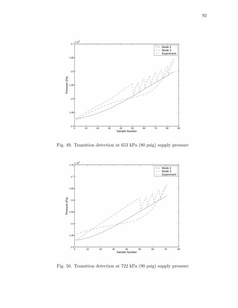
92

0 10 20 30 40 50 60 70 80 901.4

1.45

1.5

1.55

1.6

1.65

1.7x 10

5

Sample Number

Pre

ssur

e (P

a)

Mode 2Mode 3Experiment

Fig. 49. Transition detection at 653 kPa (80 psig) supply pressure

0 10 20 30 40 50 60 70 801.4

1.45

1.5

1.55

1.6

1.65

1.7

1.75x 10

5

Sample Number

Pre

ssur

e (P

a)

Mode 2Mode 3Experiment

Fig. 50. Transition detection at 722 kPa (90 psig) supply pressure

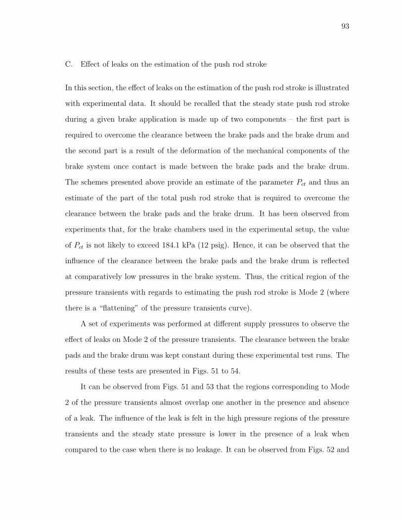
93

C. Effect of leaks on the estimation of the push rod stroke

In this section, the effect of leaks on the estimation of the push rod stroke is illustrated

with experimental data. It should be recalled that the steady state push rod stroke

during a given brake application is made up of two components – the first part is

required to overcome the clearance between the brake pads and the brake drum and

the second part is a result of the deformation of the mechanical components of the

brake system once contact is made between the brake pads and the brake drum.

The schemes presented above provide an estimate of the parameter Pct and thus an

estimate of the part of the total push rod stroke that is required to overcome the

clearance between the brake pads and the brake drum. It has been observed from

experiments that, for the brake chambers used in the experimental setup, the value

of Pct is not likely to exceed 184.1 kPa (12 psig). Hence, it can be observed that the

influence of the clearance between the brake pads and the brake drum is reflected

at comparatively low pressures in the brake system. Thus, the critical region of the

pressure transients with regards to estimating the push rod stroke is Mode 2 (where

there is a “flattening” of the pressure transients curve).

A set of experiments was performed at different supply pressures to observe the

effect of leaks on Mode 2 of the pressure transients. The clearance between the brake

pads and the brake drum was kept constant during these experimental test runs. The

results of these tests are presented in Figs. 51 to 54.

It can be observed from Figs. 51 and 53 that the regions corresponding to Mode

2 of the pressure transients almost overlap one another in the presence and absence

of a leak. The influence of the leak is felt in the high pressure regions of the pressure

transients and the steady state pressure is lower in the presence of a leak when

compared to the case when there is no leakage. It can be observed from Figs. 52 and

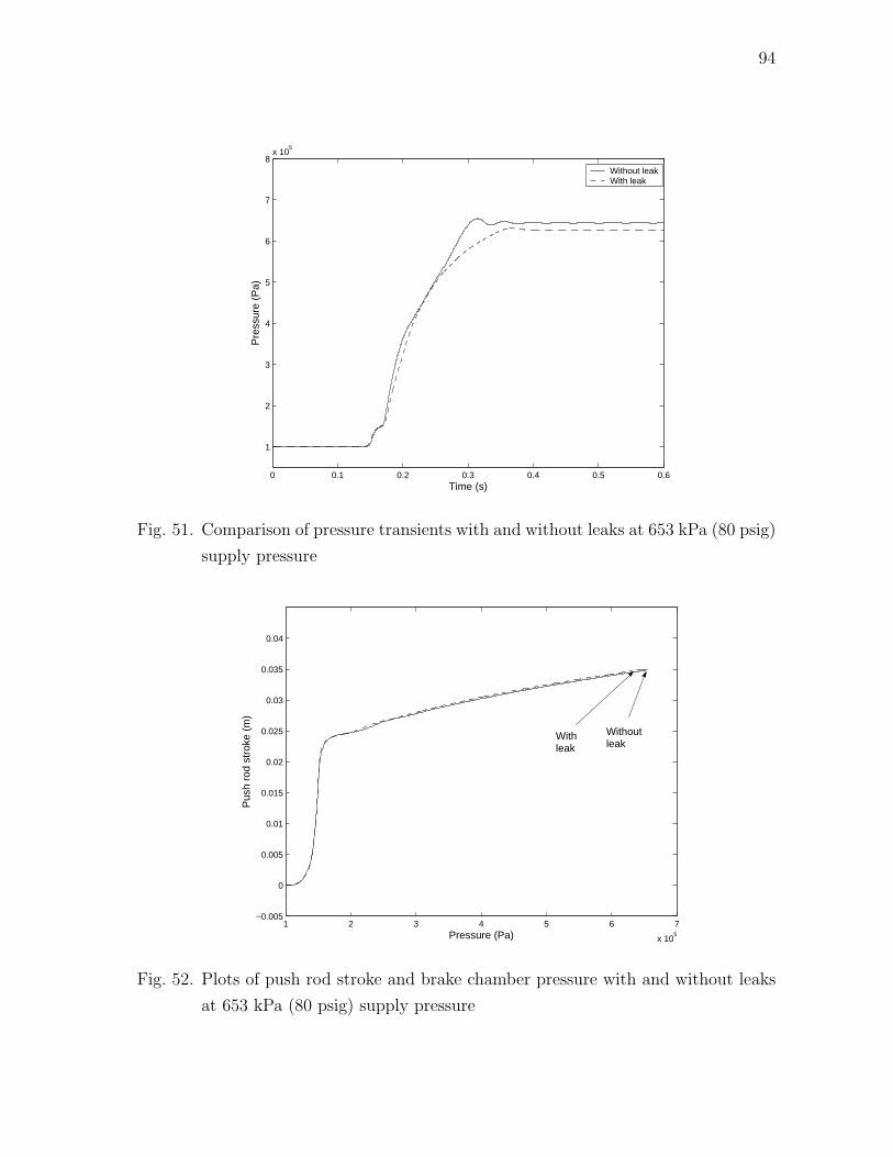
94

0 0.1 0.2 0.3 0.4 0.5 0.6

1

2

3

4

5

6

7

8x 10

5

Time (s)

Pre

ssur

e (P

a)

Without leakWith leak

Fig. 51. Comparison of pressure transients with and without leaks at 653 kPa (80 psig)

supply pressure

1 2 3 4 5 6 7

x 105

−0.005

0

0.005

0.01

0.015

0.02

0.025

0.03

0.035

0.04

Pressure (Pa)

Pus

h ro

d st

roke

(m

)

Withleak

Withoutleak

Fig. 52. Plots of push rod stroke and brake chamber pressure with and without leaks


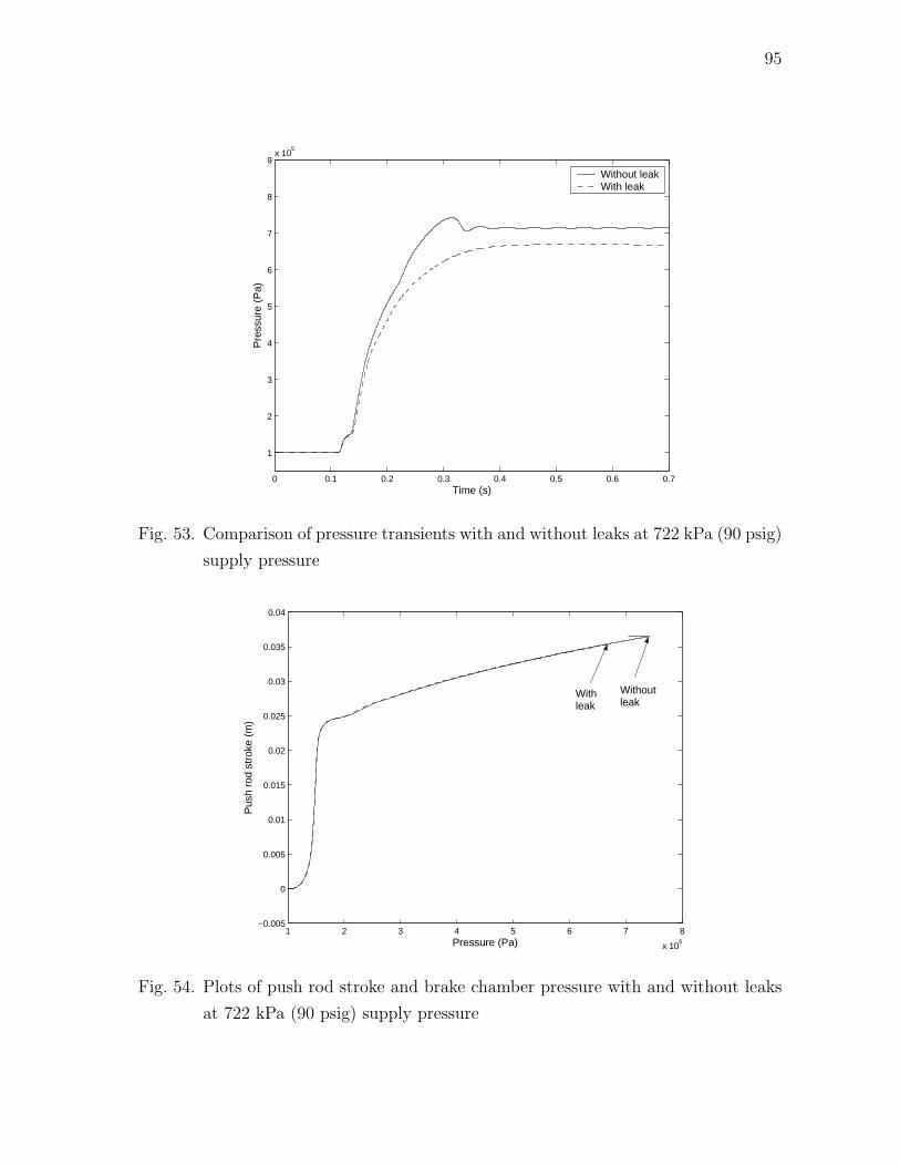
95

0 0.1 0.2 0.3 0.4 0.5 0.6 0.7

1

2

3

4

5

6

7

8

9x 10

5

Time (s)

Pre

ssur

e (P

a)

Without leakWith leak

Fig. 53. Comparison of pressure transients with and without leaks at 722 kPa (90 psig)

supply pressure

1 2 3 4 5 6 7 8

x 105

−0.005

0

0.005

0.01

0.015

0.02

0.025

0.03

0.035

0.04

Pressure (Pa)

Pus

h ro

d st

roke

(m

)

Withleak

Withoutleak

Fig. 54. Plots of push rod stroke and brake chamber pressure with and without leaks


96

54 that the steady state push rod stroke is lower in the presence of a leak due to

this reason. Also, in these two figures, the regions corresponding to Mode 2 almost

overlap one another in the presence and absence of a leak. The only major difference

is in the steady state values (indicated by arrows in these two figures). Thus, the

presence of a leak lowers the push rod stroke mainly due to the fact that the steady

state pressure in lowered.

97

CHAPTER VII

PARAMETER ESTIMATION SCHEMES FOR A CLASS OF SEQUENTIAL

HYBRID SYSTEMS

The focus of this dissertation till the previous chapter has been on air brake systems.

Based on the physical insight obtained in the development of diagnostic schemes for air

brake systems, this chapter outlines the preliminary development of a few parameter

estimation schemes for a class of sequential hybrid systems. In many physical systems,

the values of certain parameters in the equations governing the response of those

systems may not be available a priori. The values of these parameters are estimated

by providing suitable input signals to the system and measuring the corresponding

output signals. Such parameter estimation schemes often form a part of an adaptive

control system that is used for regulating the performance of the physical system. A

few examples of adaptive control include controlling robotic manipulators, aircrafts,

chemical processes, automobiles, etc. Descriptions of various techniques used in the

adaptive control of dynamic systems can be found in [97], [98].

The response of many physical systems is such that it can be represented by a

hybrid model (as is the case with the response of the pneumatic subsystem of the

air brake system). In chapter IV, some examples of automotive systems that have

been recently represented by hybrid models were presented. In [99], the authors

have presented conditions that ensure the asymptotic stability of a class of switched

systems under any switching signal. They also address the problem of identifying

classes of switching signals for which the response of the system under consideration

will be asymptotically stable. In [100], the authors consider the problem of designing

a Luenberger-like observer for a class of linear hybrid systems. They demonstrate that

the existence of a common Lyapunov function for all the modes, such that a condition

98

in the form of a Linear Matrix Inequality (LMI) is satisfied, to be sufficient for the

state estimation errors to converge asymptotically to zero. Vidal et al. [101] have

developed criteria for the observability of a class of linear discrete time hybrid systems.

The problem of switching between several controllers for a linear time invariant system

has been studied in [102].

In this chapter, the problem of designing parameter estimation schemes for a

class of sequential hybrid systems is addressed. The class of sequential hybrid systems

that is considered will be first described. Then, parameter estimation schemes for this

class of sequential hybrid systems will be presented for the case when the transition

conditions are known a priori. Then, a parameter estimation scheme will be developed

for the case when the transition conditions are not known. Specifically, the case where

the transition conditions are not known up to a constant will be considered. The

performance of these schemes will be illustrated with some examples.

A. The class of systems under study

In this chapter, the class of sequential hybrid systems whose response is described by

the following equations will be considered:

x(t) = Aix(t) + Bi [φi(u(t),y(t))θ + ψi(u(t),y(t))] , (7.1)

y(t) = Cix(t), i = 1, . . . , s, (7.2)

where x(t) ∈ Rn is the vector of state variables, u(t) ∈ R

m is the input vector,

y(t) ∈ Rp is the output vector and θ ∈ R

q is the vector of unknown (but constant)

parameters that need to be estimated. The function φi(., .) : Rm × R

p → Rr×q and

the function ψi(., .) : Rm × R

p → Rr. The dot in the above equation represents

the derivative with respect to time and the constant matrices Ai, Bi and Ci are

99

of the appropriate dimensions. The parameter s is a positive integer representing

the total number of modes. The input u(t) and the output y(t) are assumed to be

bounded. It is also assumed that for bounded u and y, and for all i = 1, . . . , s,

the functions φi(u,y) and ψi(u,y) are bounded . For convenience, the arguments

in the parenthesis shall be suppressed after their first appearance. The transition of

the system from mode i to mode (i + 1) will occur when the condition α(y) ≥ µi

is satisfied. The function α(.) : Rp → R and it is assumed that this function is a

strictly increasing function of y. There are instances of physical systems where the

transition conditions fall under this category. For example, the forward transition

from a lower gear to a higher gear will occur in an automatic transmission system

only when the vehicle speed increases. In the pneumatic subsystem of an air brake

system, the forward transition from one mode to the following mode occurs only when

the pressure in the brake chamber increases and the backward transition from one

mode to the previous mode will occur only when the pressure in the brake chamber

decreases. In modeling the flow of traffic, the number of vehicles in a section must

increase to cause a forward transition to a more congested regime [103]. The reverse

transition from mode (i+1) to mode i will occur when α(y) < µi. In section B of this

chapter, it will be assumed that the values of µi, i = 1, . . . , (s− 1) are known a priori

so that a complete knowledge of the transition conditions is available. In section C

of this chapter, the case where the transition conditions are unknown, in the sense

that the values of µi, i = 1, . . . , (s − 1) are not known, will be considered. It should

be noted that Eq. (7.1) is linear in θ. This system is illustrated in Fig. 55.

The problem under study in section B of this chapter can be stated as follows:

Consider the class of systems described by Eqs. (7.1) and (7.2). Given the input u,

the output y and a complete knowledge of the transition conditions (i.e., the values

of µi, i = 1, . . . , (s − 1), are known), obtain a parameter estimation scheme that will

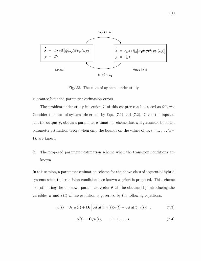
100

Fig. 55. The class of systems under study

guarantee bounded parameter estimation errors.

The problem under study in section C of this chapter can be stated as follows:

Consider the class of systems described by Eqs. (7.1) and (7.2). Given the input u

and the output y, obtain a parameter estimation scheme that will guarantee bounded

parameter estimation errors when only the bounds on the values of µi, i = 1, . . . , (s−1), are known.

B. The proposed parameter estimation scheme when the transition conditions are

known

In this section, a parameter estimation scheme for the above class of sequential hybrid

systems when the transition conditions are known a priori is proposed. This scheme

for estimating the unknown parameter vector θ will be obtained by introducing the

variables w and y(t) whose evolution is governed by the following equations:

w(t) = Aiw(t) + Bi

[φi(u(t),y(t))θ(t) + ψi(u(t),y(t))

], (7.3)

y(t) = Ciw(t), i = 1, . . . , s, (7.4)

101

where θ(t) is the estimate of θ at time t. Next, the following variables are defined as:

eo(t) = y(t) − y(t), (7.5)

eθ(t) = θ∗ − θ(t), (7.6)

ex(t) = x(t) − w(t), (7.7)

where eθ(t) is the parameter estimation error and θ∗ is the vector of the actual pa-

rameter values. The variable eo(t) will be referred to as the output identification

error. The following proposition then provides sufficient conditions and a parameter

update scheme for estimating θ.

Proposition 1: Consider the sequential hybrid system whose governing equa-

tions in the ith mode are given by Eqs. (7.1) and (7.2). Let a positive definite function

V (t) be defined through

V (t) = Peo.eo +1

2eθ.eθ, (7.8)

where P is a symmetric positive definite matrix. If for each i = 1, . . . , s, there exists

a symmetric semi-positive definite matrix Qi such that

CTi PCiAi + AT

i CiPCi = −Qi, i = 1, . . . , s, (7.9)

then choosing

˙θ = 2 [PCiBiφi]

T eo, i = 1, . . . , s, (7.10)

will lead to the parameter estimation error and the output identification error being

bounded.

Proof: From the above definition of V , one obtains

V =[CT

i PCiAi + ATi CiPCi

]ex.ex +

[2 [PCiBiφi]

T eo + eθ

].eθ. (7.11)

102

Using Eqs. (7.9) and (7.10), the above equation reduces to

V = −Qiex.ex. (7.12)

Since Qi is a symmetric semi-positive definite matrix for each i = 1, . . . , s, it can be

observed that for all t > 0, V ≤ 0 along the system trajectories given by Eqs. (7.1)–

(7.4) and Eq. (7.10). Thus, if one starts with non-zero initial conditions for eo and

eθ, choosing a parameter update scheme given by Eq. (7.10) will lead to a bounded

parameter estimation error and a bounded output identification error.

�

Remarks: The following features of the proposed parameter estimation scheme

must be noted:

1. Let the system be in mode i at time t = 0 and let the system switch to mode

(i + 1) at time t = T . Then, the values of the parameter estimates obtained

at t = T from the parameter estimation scheme implemented in mode i will be

taken as the initial values for the parameter estimation scheme implemented in

mode (i + 1).

2. It can be noted that the above scheme allows for the use of different matrices

Qi for different modes. The matrices P and Qi can be regarded as design pa-

rameters in obtaining a parameter estimation scheme for the sequential hybrid

system under study. If it is possible to obtain a common matrix Q that satisfies

Eq. (7.9) for all i = 1, . . . , s, then that matrix can be used for all the modes. If

not, the proposed parametric scheme provides the flexibility of choosing a dif-

ferent matrix Qi for each mode. This feature will be illustrated in the following

examples.

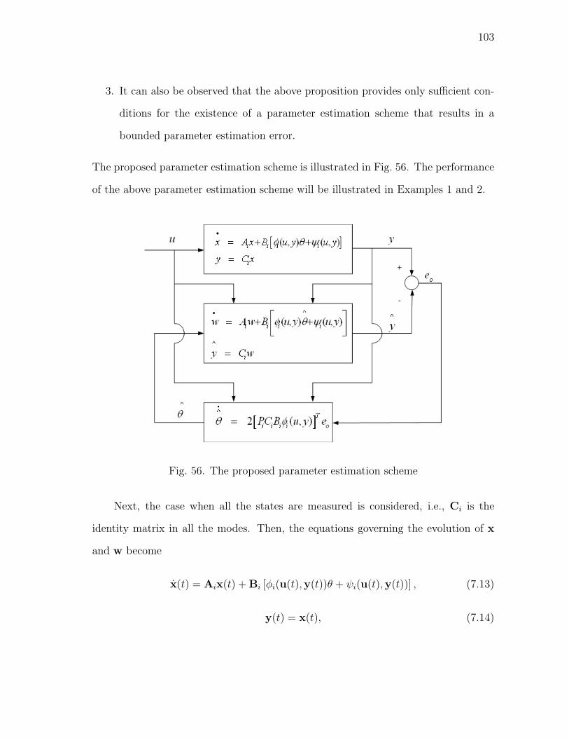
103

3. It can also be observed that the above proposition provides only sufficient con-

ditions for the existence of a parameter estimation scheme that results in a

bounded parameter estimation error.

The proposed parameter estimation scheme is illustrated in Fig. 56. The performance

of the above parameter estimation scheme will be illustrated in Examples 1 and 2.

Fig. 56. The proposed parameter estimation scheme

Next, the case when all the states are measured is considered, i.e., Ci is the

identity matrix in all the modes. Then, the equations governing the evolution of x

and w become

x(t) = Aix(t) + Bi [φi(u(t),y(t))θ + ψi(u(t),y(t))] , (7.13)

y(t) = x(t), (7.14)

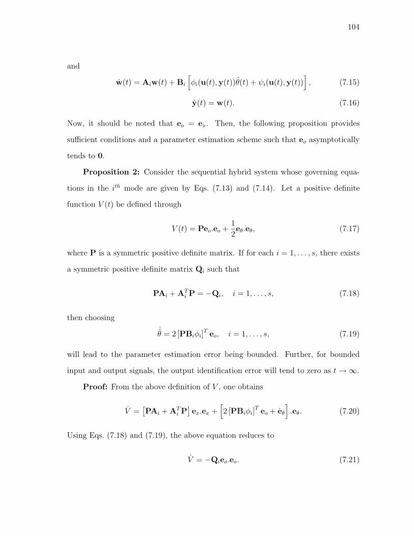
104

and

w(t) = Aiw(t) + Bi

[φi(u(t),y(t))θ(t) + ψi(u(t),y(t))

], (7.15)

y(t) = w(t). (7.16)

Now, it should be noted that eo = ex. Then, the following proposition provides

sufficient conditions and a parameter estimation scheme such that eo asymptotically

tends to 0.

Proposition 2: Consider the sequential hybrid system whose governing equa-

tions in the ith mode are given by Eqs. (7.13) and (7.14). Let a positive definite

function V (t) be defined through

V (t) = Peo.eo +1

2eθ.eθ, (7.17)

where P is a symmetric positive definite matrix. If for each i = 1, . . . , s, there exists

a symmetric positive definite matrix Qi such that

PAi + ATi P = −Qi, i = 1, . . . , s, (7.18)

then choosing

˙θ = 2 [PBiφi]

T eo, i = 1, . . . , s, (7.19)

will lead to the parameter estimation error being bounded. Further, for bounded

input and output signals, the output identification error will tend to zero as t → ∞.

Proof: From the above definition of V , one obtains

V =[PAi + AT

i P]ex.ex +

[2 [PBiφi]

T eo + eθ

].eθ. (7.20)

Using Eqs. (7.18) and (7.19), the above equation reduces to

V = −Qieo.eo. (7.21)

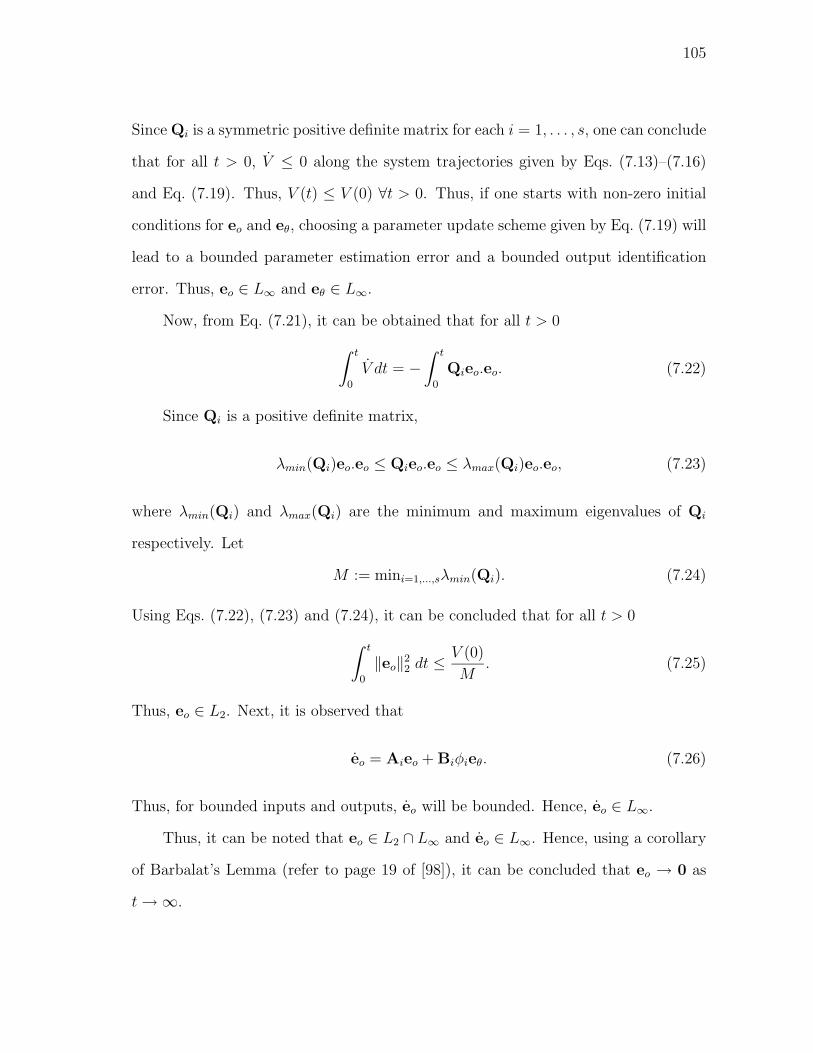
105

Since Qi is a symmetric positive definite matrix for each i = 1, . . . , s, one can conclude

that for all t > 0, V ≤ 0 along the system trajectories given by Eqs. (7.13)–(7.16)

and Eq. (7.19). Thus, V (t) ≤ V (0) ∀t > 0. Thus, if one starts with non-zero initial

conditions for eo and eθ, choosing a parameter update scheme given by Eq. (7.19) will

lead to a bounded parameter estimation error and a bounded output identification

error. Thus, eo ∈ L∞ and eθ ∈ L∞.

Now, from Eq. (7.21), it can be obtained that for all t > 0

∫ t

0

V dt = −∫ t

0

Qieo.eo. (7.22)

Since Qi is a positive definite matrix,

λmin(Qi)eo.eo ≤ Qieo.eo ≤ λmax(Qi)eo.eo, (7.23)

where λmin(Qi) and λmax(Qi) are the minimum and maximum eigenvalues of Qi

respectively. Let

M := mini=1,...,sλmin(Qi). (7.24)

Using Eqs. (7.22), (7.23) and (7.24), it can be concluded that for all t > 0

∫ t

0

‖eo‖22 dt ≤ V (0)

M. (7.25)

Thus, eo ∈ L2. Next, it is observed that

eo = Aieo + Biφieθ. (7.26)

Thus, for bounded inputs and outputs, eo will be bounded. Hence, eo ∈ L∞.

Thus, it can be noted that eo ∈ L2 ∩ L∞ and eo ∈ L∞. Hence, using a corollary

of Barbalat’s Lemma (refer to page 19 of [98]), it can be concluded that eo → 0 as

t → ∞.

106

�

It should be noted that if a common Q that satisfies Eq. (7.18) exists for all the

modes, then it can be used for obtaining the parameter update equations. Otherwise,

the above parameter estimation scheme provides the flexibility of choosing a different

Qi in each mode such that Eq. (7.18) is satisfied. The performance of this scheme is

illustrated in Example 3.

1. Example 1

In this example, the system illustrated in Fig. 57 will be considered. Let x be the

displacement of the mass m from its initial position. A force F is applied on it to

move it from its initial position and let L denote the value of x at which the mass will

make contact with the second set of spring and dashpot. There are two modes in this

system – mode 1 is described by the condition x < L and mode 2 is described by the

condition x ≥ L. It is assumed that all the springs and dashpots are linear and that

both the displacement (x) and the velocity (x) are measured. Let it be supposed that

the values of c1 and k2 are unknown and need to be estimated. Let the true values

of all the parameters be m = 1 kg, k1 = 3 N/m, c1 = 0.5 Ns/m, k2 = 1 N/m, c2 = 2

Ns/m and L = 0.2 m.

The equation of motion of the system in mode 1 is given by

mx = F − k1x − c1x, (7.27)

and the equation of motion of the system in mode 2 is given by

mx = F − k1x − c1x − k2(x − L) − c2x. (7.28)

The equation of motion in mode 1 can be re-written as (in order to identify it with

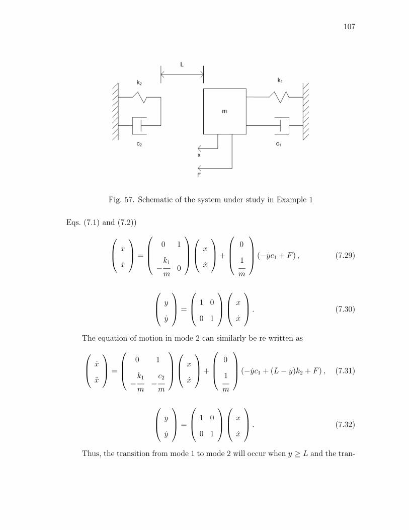
107

Fig. 57. Schematic of the system under study in Example 1

Eqs. (7.1) and (7.2))

x

x

=

0 1

−k1

m0

x

x

+

0

1

m

(−yc1 + F ) , (7.29)

y

y

=

1 0

0 1

x

x

. (7.30)

The equation of motion in mode 2 can similarly be re-written as

x

x

=

0 1

−k1

m−

c2

m

x

x

+

0

1

m

(−yc1 + (L − y)k2 + F ) , (7.31)

y

y

=

1 0

0 1

x

x

. (7.32)

Thus, the transition from mode 1 to mode 2 will occur when y ≥ L and the tran-

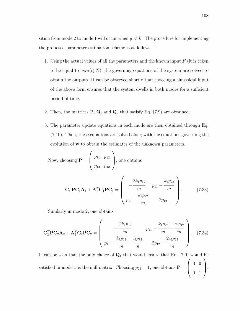
108

sition from mode 2 to mode 1 will occur when y < L. The procedure for implementing

the proposed parameter estimation scheme is as follows:

1. Using the actual values of all the parameters and the known input F (it is taken

to be equal to 5sin(t) N), the governing equations of the system are solved to

obtain the outputs. It can be observed shortly that choosing a sinusoidal input

of the above form ensures that the system dwells in both modes for a sufficient

period of time.

2. Then, the matrices P, Q1 and Q2 that satisfy Eq. (7.9) are obtained.

3. The parameter update equations in each mode are then obtained through Eq.

(7.10). Then, these equations are solved along with the equations governing the

evolution of w to obtain the estimates of the unknown parameters.

Now, choosing P =

p11 p12

p12 p22

, one obtains

CT1 PC1A1 + AT

1 C1PC1 =

−2k1p12

mp11 −

k1p22

m

p11 −k1p22

m2p12

. (7.33)

Similarly in mode 2, one obtains

CT2 PC2A2 + AT

2 C2PC2 =

−2k1p12

mp11 −

k1p22

m−

c2p12

m

p11 −k1p22

m−

c2p12

m2p12 −

2c2p22

m

. (7.34)

It can be seen that the only choice of Q1 that would ensure that Eq. (7.9) would be

satisfied in mode 1 is the null matrix. Choosing p22 = 1, one obtains P =

3 0

0 1

.

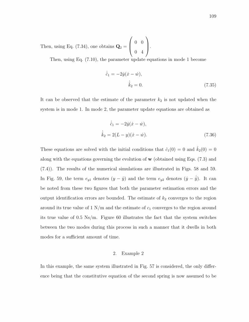
109

Then, using Eq. (7.34), one obtains Q2 =

0 0

0 4

.

Then, using Eq. (7.10), the parameter update equations in mode 1 become

˙c1 = −2y(x − w),

˙k2 = 0. (7.35)

It can be observed that the estimate of the parameter k2 is not updated when the

system is in mode 1. In mode 2, the parameter update equations are obtained as

˙c1 = −2y(x − w),

˙k2 = 2(L − y)(x − w). (7.36)

These equations are solved with the initial conditions that c1(0) = 0 and k2(0) = 0

along with the equations governing the evolution of w (obtained using Eqs. (7.3) and

(7.4)). The results of the numerical simulations are illustrated in Figs. 58 and 59.

In Fig. 59, the term ey1 denotes (y − y) and the term ey2 denotes (y − ˙y). It can

be noted from these two figures that both the parameter estimation errors and the

output identification errors are bounded. The estimate of k2 converges to the region

around its true value of 1 N/m and the estimate of c1 converges to the region around

its true value of 0.5 Ns/m. Figure 60 illustrates the fact that the system switches

between the two modes during this process in such a manner that it dwells in both

modes for a sufficient amount of time.

2. Example 2

In this example, the same system illustrated in Fig. 57 is considered, the only differ-

ence being that the constitutive equation of the second spring is now assumed to be

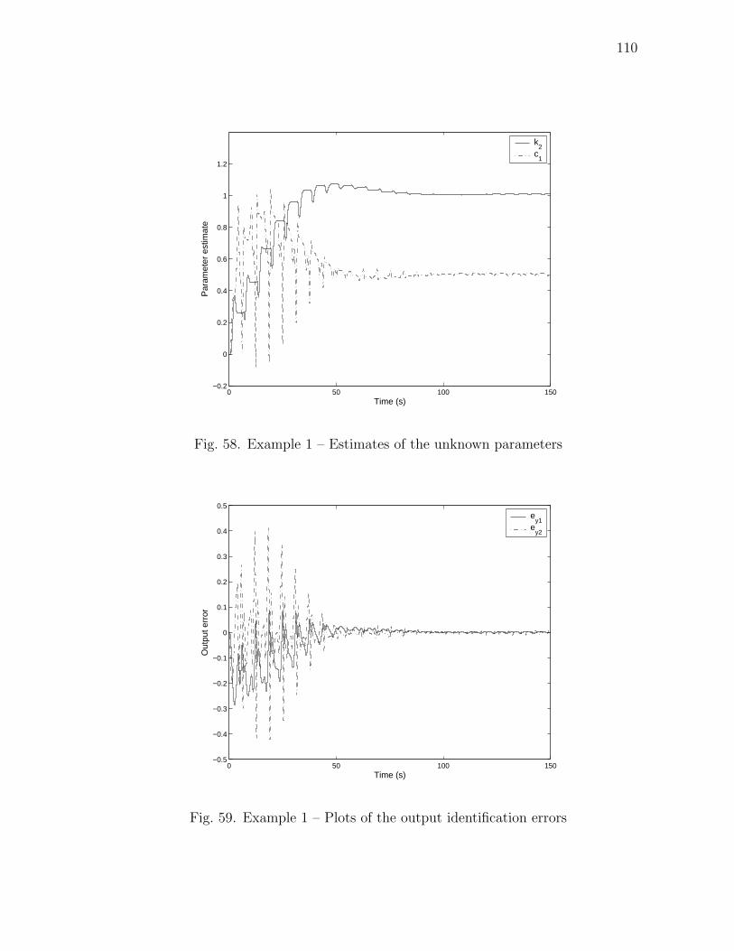
110

0 50 100 150−0.2

0

0.2

0.4

0.6

0.8

1

1.2

Time (s)

Par

amet

er e

stim

ate

k2

c1

Fig. 58. Example 1 – Estimates of the unknown parameters

0 50 100 150−0.5

−0.4

−0.3

−0.2

−0.1

0

0.1

0.2

0.3

0.4

0.5

Time (s)

Out

put e

rror

ey1

ey2

Fig. 59. Example 1 – Plots of the output identification errors

111

0 50 100 1500

0.5

1

1.5

2

2.5

3

Time (s)

Mod

e

Fig. 60. Example 1 – Switching between the two modes

given by Fs2 = k2(x − L)3, where Fs2 is the force applied on it. The effect of this

non-linearity on the performance of the proposed parameter estimation scheme will

be observed. It is still assumed that the true values of all the parameters are m = 1

kg, k1 = 3 N/m, c1 = 0.5 Ns/m, k2 = 1 N/m, c2 = 2 Ns/m and L = 0.2 m. It is once

again assumed that the values of c1 and k2 are unknown and need to be estimated.

The equation of motion of the system in mode 1 is given by

mx = F − k1x − c1x, (7.37)

and the equation of motion of the system in mode 2 is given by

mx = F − k1x − c1x − k2(x − L)3 − c2x. (7.38)

Following the same procedure as in the previous example and making the same

choices for P, Q1 and Q2, the parameter update equations (using Eq. (7.10)) in mode

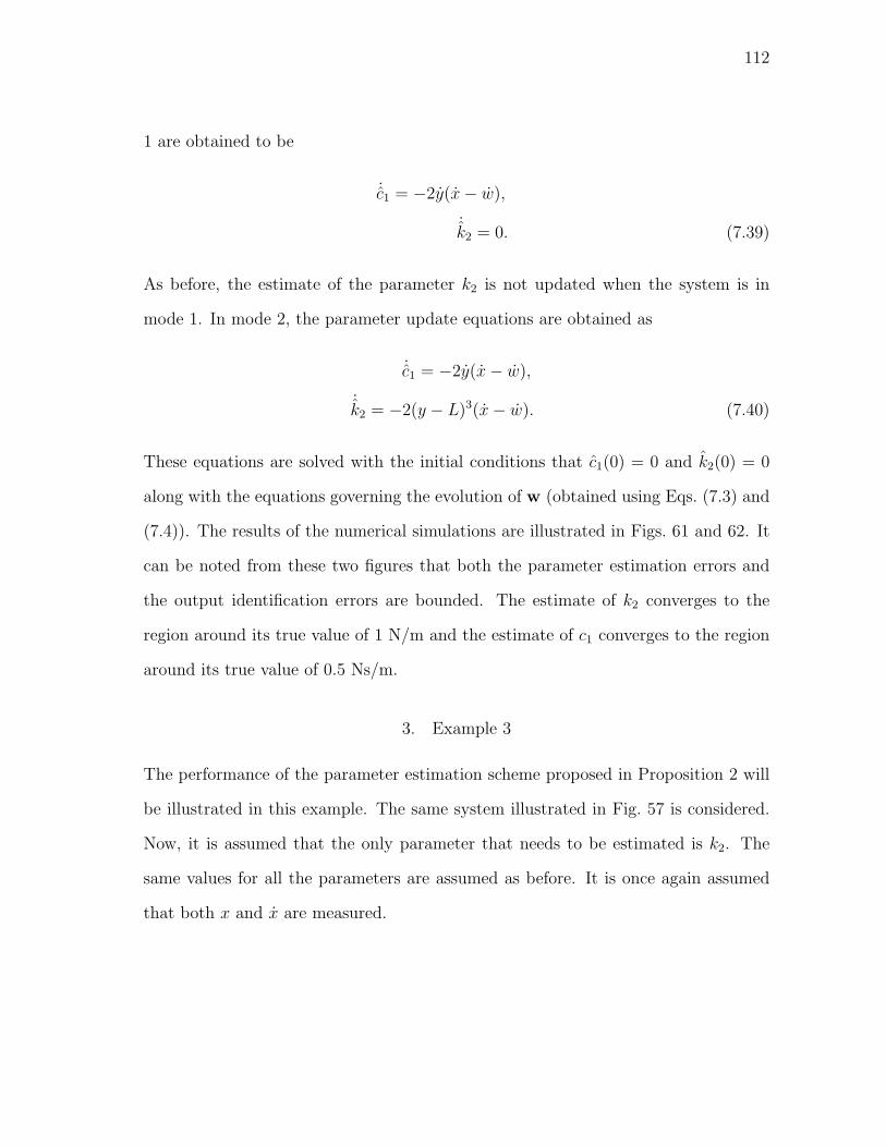
112

1 are obtained to be

˙c1 = −2y(x − w),

˙k2 = 0. (7.39)

As before, the estimate of the parameter k2 is not updated when the system is in

mode 1. In mode 2, the parameter update equations are obtained as

˙c1 = −2y(x − w),

˙k2 = −2(y − L)3(x − w). (7.40)

These equations are solved with the initial conditions that c1(0) = 0 and k2(0) = 0

along with the equations governing the evolution of w (obtained using Eqs. (7.3) and

(7.4)). The results of the numerical simulations are illustrated in Figs. 61 and 62. It

can be noted from these two figures that both the parameter estimation errors and

the output identification errors are bounded. The estimate of k2 converges to the

region around its true value of 1 N/m and the estimate of c1 converges to the region

around its true value of 0.5 Ns/m.

3. Example 3

The performance of the parameter estimation scheme proposed in Proposition 2 will

be illustrated in this example. The same system illustrated in Fig. 57 is considered.

Now, it is assumed that the only parameter that needs to be estimated is k2. The

same values for all the parameters are assumed as before. It is once again assumed

that both x and x are measured.

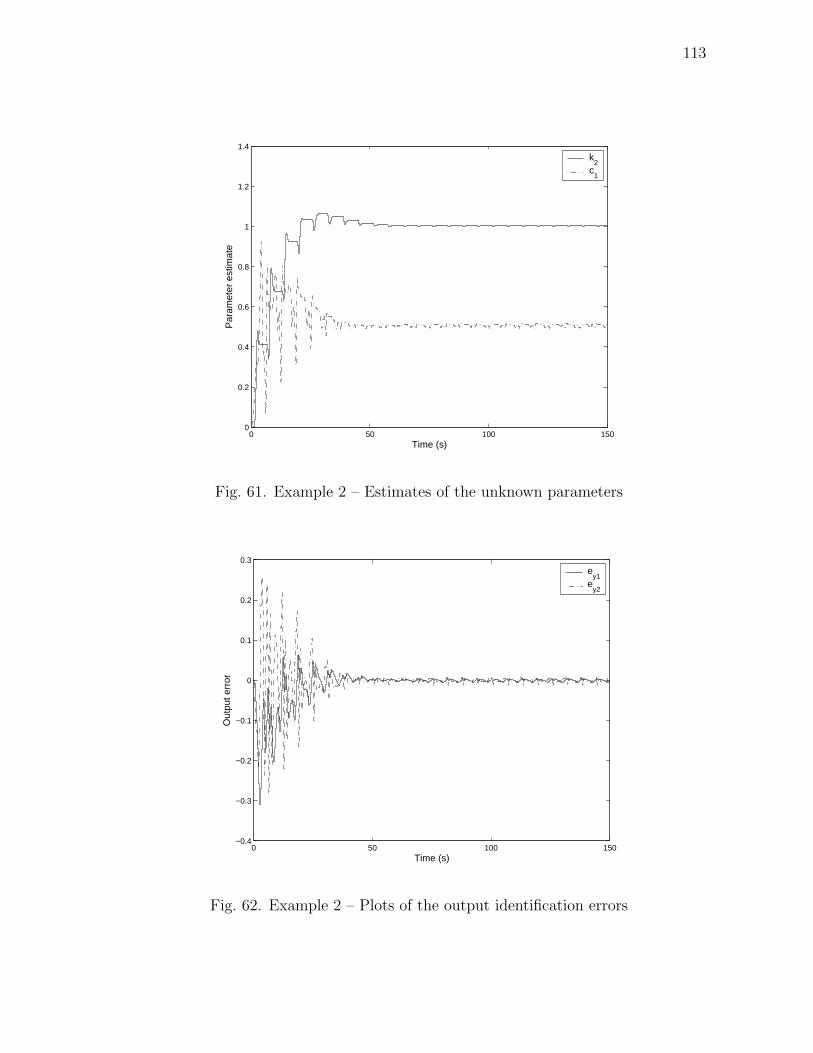
113

0 50 100 1500

0.2

0.4

0.6

0.8

1

1.2

1.4

Time (s)

Par

amet

er e

stim

ate

k2

c1

Fig. 61. Example 2 – Estimates of the unknown parameters

0 50 100 150−0.4

−0.3

−0.2

−0.1

0

0.1

0.2

0.3

Time (s)

Out

put e

rror

ey1

ey2


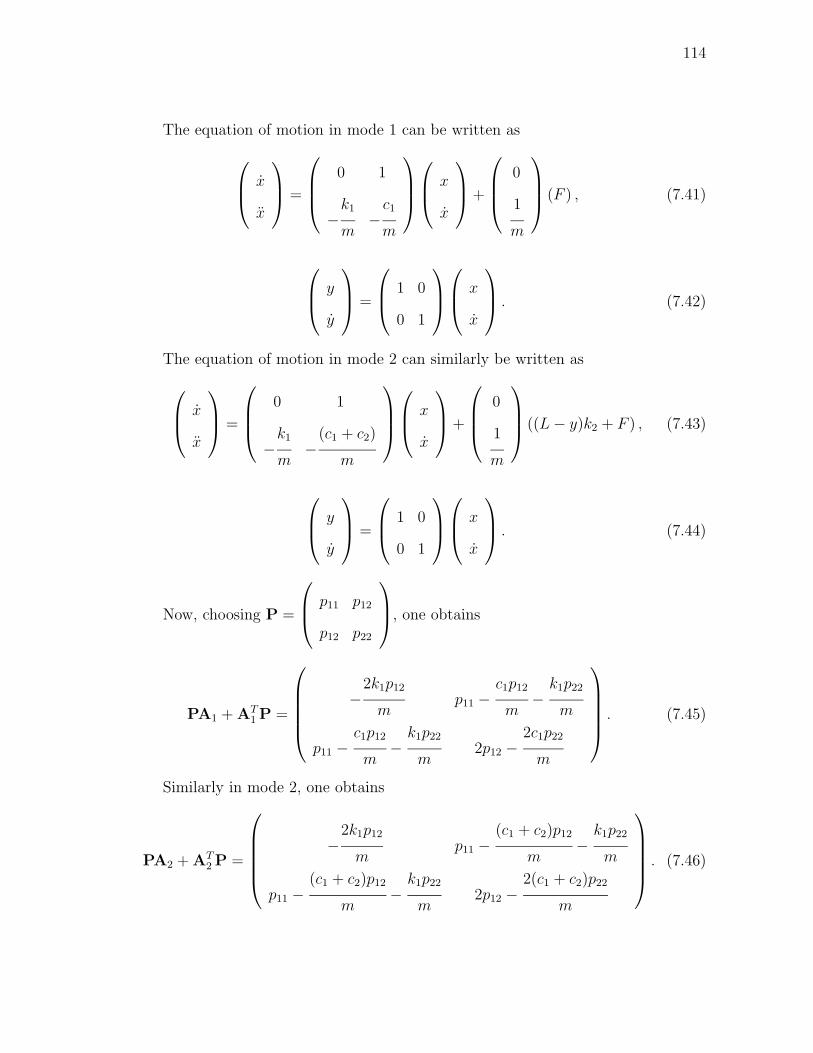
114

The equation of motion in mode 1 can be written as

x

x

=

0 1

−k1

m−

c1

m

x

x

+

0

1

m

(F ) , (7.41)

y

y

=

1 0

0 1

x

x

. (7.42)

The equation of motion in mode 2 can similarly be written as

x

x

=

0 1

−k1

m−

(c1 + c2)

m

x

x

+

0

1

m

((L − y)k2 + F ) , (7.43)

y

y

=

1 0

0 1

x

x

. (7.44)

Now, choosing P =

p11 p12

p12 p22

, one obtains

PA1 + AT1 P =

−2k1p12

mp11 −

c1p12

m−

k1p22

m

p11 −c1p12

m−

k1p22

m2p12 −

2c1p22

m

. (7.45)


PA2 + AT2 P =

−2k1p12

mp11 −

(c1 + c2)p12

m−

k1p22

m

p11 −(c1 + c2)p12

m−

k1p22

m2p12 −

2(c1 + c2)p22

m

. (7.46)

115

Choosing P =

9.5 1

1 3

, Q1 =

6 0

0 1

and Q2 =

6 2

2 13

ensures that

Eq. (7.18) is satisfied for both modes. It can be noted that all the conditions listed in

Proposition 2 are satisfied in this case. Thus, using Eq. (7.19), the parameter update

equation in mode 1 is obtained to be

˙k2 = 0. (7.47)

The parameter update equation in mode 2 is obtained to be

˙k2 = 2(L − y)(x − w) + 6(L − y)(x − w). (7.48)

The results of the numerical simulations in this case are presented in Figs. 63 and 64.

It can be observed that the output identification errors tend to zero asymptotically

and the estimate of the parameter k2 tends very nearly to its true value of 1 N/m. A

faster convergence of the parameter estimate to the actual value is observed in this

case when compared with Example 1 (compare with Figs. 58 and 59).

C. The proposed parameter estimation scheme when the transition conditions are

unknown

In this section, a parameter estimation scheme is developed for the class of systems

given by Eqs. (7.13) and (7.14) when the transition conditions are not known. In

particular, it will be assumed that the values of µi, i = 1, . . . , (s − 1), are not known

but the bounds on each of them are known. In this case, the vector of unknown

parameters θ also includes µ1, . . . , µs−1. It is assumed that α(.) is a strictly increasing

function of y. It is assumed that the initial mode of the system is known. The lower

bound on µi is denoted by βi and the upper bound on µi is denoted by δi. It is

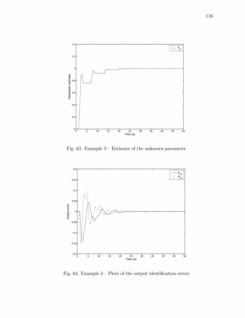
116

0 5 10 15 20 25 30 35 40 45 500

0.2

0.4

0.6

0.8

1

1.2

1.4

Time (s)

Par

amet

er e

stim

ate

k2

Fig. 63. Example 3 – Estimate of the unknown parameter

0 5 10 15 20 25 30 35 40 45 50−0.2

−0.15

−0.1

−0.05

0

0.05

0.1

0.15

0.2

Time (s)

Out

put e

rror

ey1

ey2


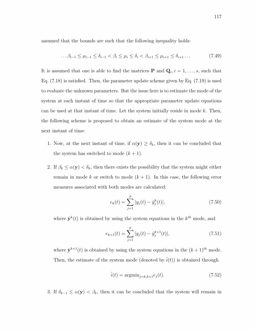
117

assumed that the bounds are such that the following inequality holds:

. . . βi−1 ≤ µi−1 ≤ δi−1 < βi ≤ µi ≤ δi < βi+1 ≤ µi+1 ≤ δi+1 . . . (7.49)

It is assumed that one is able to find the matrices P and Qi, i = 1, . . . , s, such that

Eq. (7.18) is satisfied. Then, the parameter update scheme given by Eq. (7.19) is used

to evaluate the unknown parameters. But the issue here is to estimate the mode of the

system at each instant of time so that the appropriate parameter update equations

can be used at that instant of time. Let the system initially reside in mode k. Then,

the following scheme is proposed to obtain an estimate of the system mode at the

next instant of time:

1. Now, at the next instant of time, if α(y) ≥ δk, then it can be concluded that

the system has switched to mode (k + 1).

2. If βk ≤ α(y) < δk, then there exists the possibility that the system might either

remain in mode k or switch to mode (k + 1). In this case, the following error

measures associated with both modes are calculated:

ek(t) =

p∑j=1

|yj(t) − ykj (t)|, (7.50)

where yk(t) is obtained by using the system equations in the kth mode, and

ek+1(t) =

p∑j=1

|yj(t) − yk+1j (t)|, (7.51)

where yk+1(t) is obtained by using the system equations in the (k + 1)th mode.

Then, the estimate of the system mode (denoted by i(t)) is obtained through

i(t) = argminj=k,k+1ej(t). (7.52)

3. If δk−1 ≤ α(y) < βk, then it can be concluded that the system will remain in

118

mode k at the next instant of time.

4. If βk−1 ≤ α(y) < δk−1, then there exists the possibility that the system might

either remain in mode k or switch to mode (k − 1). In this case, the following

error measures associated with both modes are calculated:

ek(t) =

p∑j=1

|yj(t) − ykj (t)|, (7.53)

where yk(t) is obtained by using the system equations in the kth mode, and

ek−1(t) =

p∑j=1

|yj(t) − yk−1j (t)|, (7.54)

where yk−1(t) is obtained by using the system equations in the (k − 1)th mode.

Then, the estimate of the system mode (denoted by i(t)) is obtained through

i(t) = argminj=k,k−1ej(t). (7.55)

5. If α(y) < βk−1, then it can be concluded that the system has switched to mode

(k − 1).

Once an estimate of the mode is obtained, the parameter update equations corre-

sponding to that estimated mode are used to obtain the parameter estimates at the

next instant of time. The above steps are repeated at each instant of time to obtain

estimates of both the system modes and the parameters. This scheme is illustrated

in the following example.

1. Example 4

The performance of the parameter estimation scheme proposed above is illustrated

in this example. The same system illustrated in Fig. 57 is considered. Now, it is

assumed that the only parameter that needs to be estimated is L. The same values

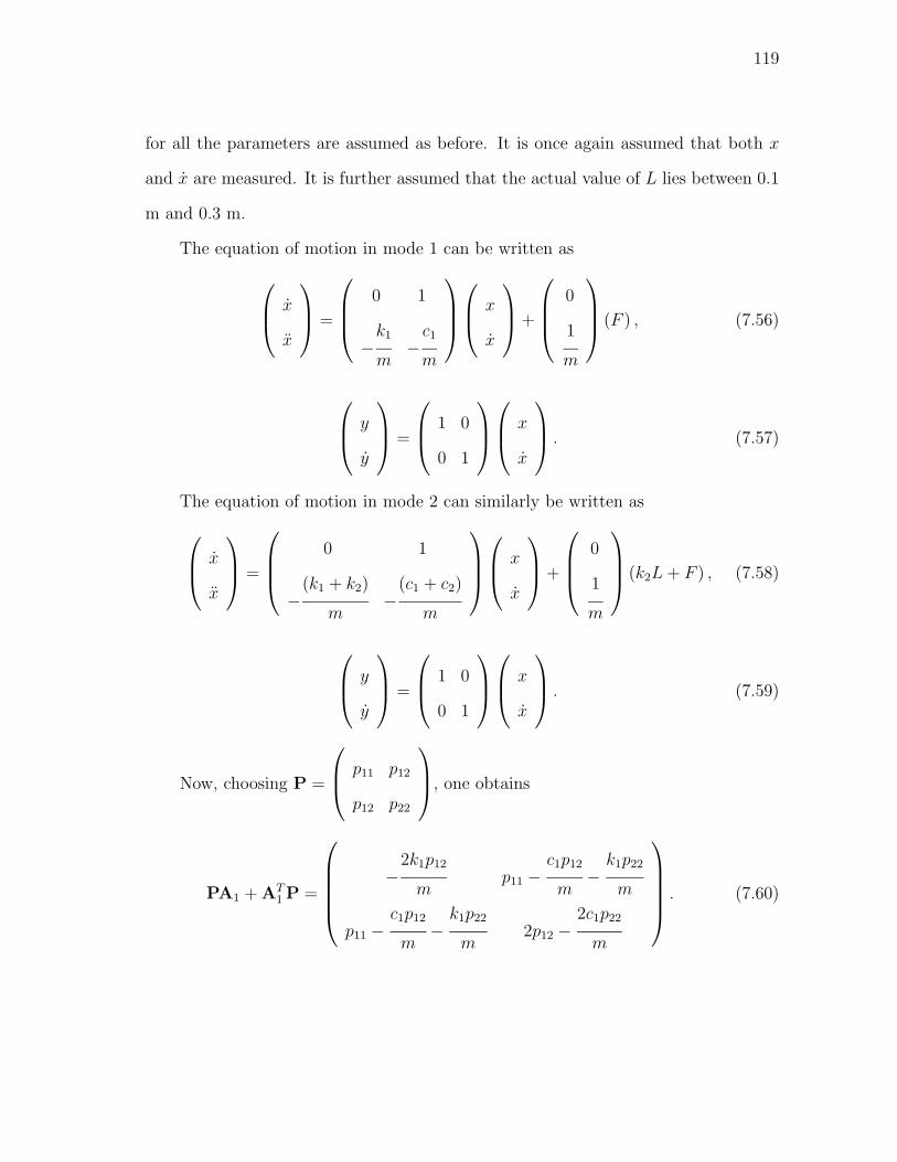
119

for all the parameters are assumed as before. It is once again assumed that both x

and x are measured. It is further assumed that the actual value of L lies between 0.1

m and 0.3 m.

The equation of motion in mode 1 can be written as

x

x

=

0 1

−k1

m−

c1

m

x

x

+

0

1

m

(F ) , (7.56)

y

y

=

1 0

0 1

x

x

. (7.57)

The equation of motion in mode 2 can similarly be written as

x

x

=

0 1

−(k1 + k2)

m−

(c1 + c2)

m

x

x

+

0

1

m

(k2L + F ) , (7.58)

y

y

=

1 0

0 1

x

x

. (7.59)

Now, choosing P =

p11 p12

p12 p22

, one obtains

PA1 + AT1 P =

−2k1p12

mp11 −

c1p12

m−

k1p22

m

p11 −c1p12

m−

k1p22

m2p12 −

2c1p22

m

. (7.60)

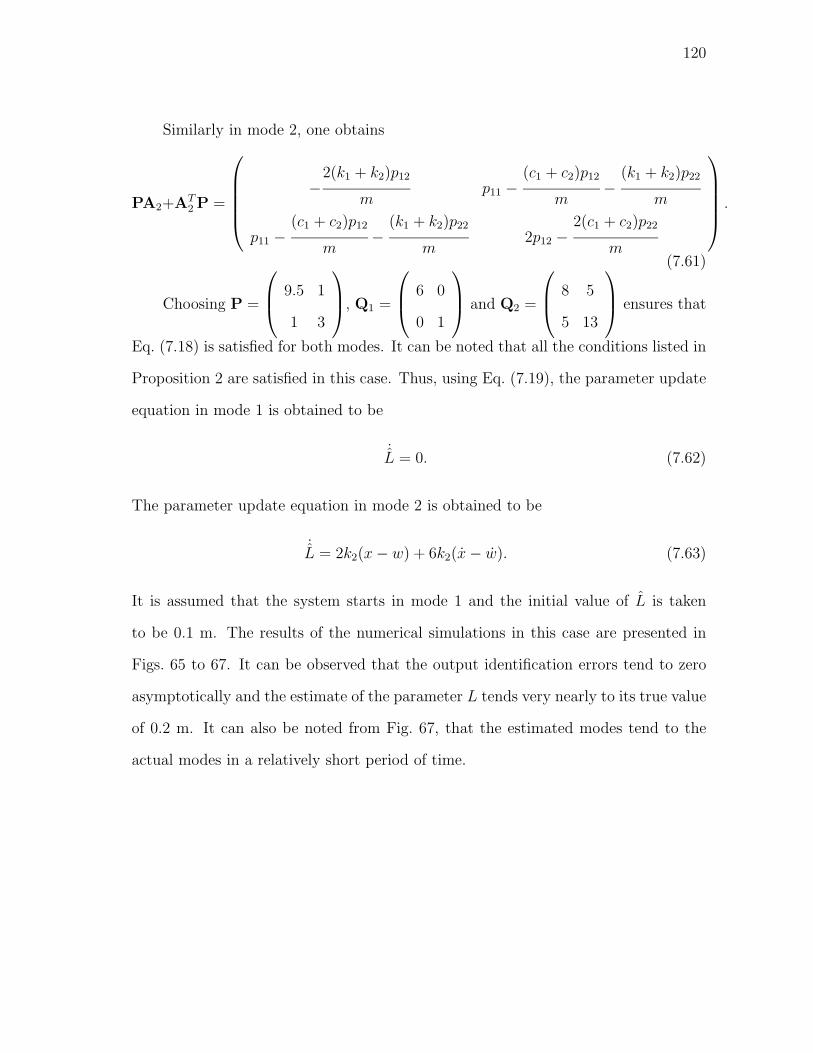
120


PA2+AT2 P =

−2(k1 + k2)p12

mp11 −

(c1 + c2)p12

m−

(k1 + k2)p22

m

p11 −(c1 + c2)p12

m−

(k1 + k2)p22

m2p12 −

2(c1 + c2)p22

m

.

(7.61)

Choosing P =

9.5 1

1 3

, Q1 =

6 0

0 1

and Q2 =

8 5

5 13

ensures that

Eq. (7.18) is satisfied for both modes. It can be noted that all the conditions listed in

Proposition 2 are satisfied in this case. Thus, using Eq. (7.19), the parameter update

equation in mode 1 is obtained to be

˙L = 0. (7.62)

The parameter update equation in mode 2 is obtained to be

˙L = 2k2(x − w) + 6k2(x − w). (7.63)

It is assumed that the system starts in mode 1 and the initial value of L is taken

to be 0.1 m. The results of the numerical simulations in this case are presented in

Figs. 65 to 67. It can be observed that the output identification errors tend to zero

asymptotically and the estimate of the parameter L tends very nearly to its true value

of 0.2 m. It can also be noted from Fig. 67, that the estimated modes tend to the

actual modes in a relatively short period of time.

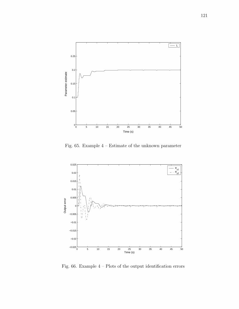
121

0 5 10 15 20 25 30 35 40 45 500

0.05

0.1

0.15

0.2

0.25

Time (s)

Par

amet

er e

stim

ate

L

Fig. 65. Example 4 – Estimate of the unknown parameter

0 5 10 15 20 25 30 35 40 45 50−0.025

−0.02

−0.015

−0.01

−0.005

0

0.005

0.01

0.015

0.02

0.025

Time (s)

Out

put e

rror

ey1

ey2


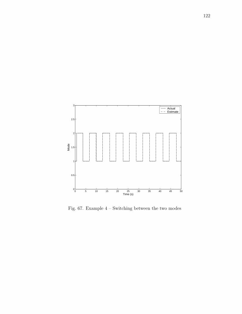
122

0 5 10 15 20 25 30 35 40 45 500

0.5

1

1.5

2

2.5

3

Time (s)

Mod

e

ActualEstimate

Fig. 67. Example 4 – Switching between the two modes

123

CHAPTER VIII

CONCLUSIONS

In this dissertation, model-based diagnostic schemes have been presented that will

automatically monitor the air brake system used in commercial vehicles for leaks and

out-of-adjustment of push rods. A model for predicting the pressure transients in the

brake chamber of the air brake system by using the measurements of the treadle valve

plunger displacement and the supply pressure to the treadle valve has been presented.

The diagnostic schemes have been developed to conform to existing FMCSA guidelines

for inspecting the air brake system. The diagnostic scheme proposed for leak detection

utilizes the measurement of the steady state brake chamber pressure and compares it

with the supply pressure to infer the presence or the absence of leakage. Two schemes

have been proposed to estimate the stroke of the push rod. These schemes utilize the

hybrid model for the pressure transients to obtain an estimate of the push rod stroke.

These schemes present a method for estimating unknown parameters and detecting

transitions in sequential hybrid systems. A general class of sequential hybrid systems

has been considered and parameter estimation schemes have been developed for them.

The performance of these schemes has been illustrated with a few examples.

To summarize, the diagnostic schemes presented in this dissertation utilize the

data collected during a full brake application carried out with a supply pressure

between 653 kPa (80 psig) and 722 kPa (90 psig). The push rod stroke required to

overcome the clearance between the brake pads and the brake drum is estimated using

the hybrid model for the pressure transients. It has been observed that the effect of

this portion of the push rod stroke is reflected in the low pressure region of the pressure

transients (within a pressure of 184.1 kPa (12 psig) in the brake chamber). The push

rod stroke due to the deformation of the mechanical components of the brake system

124

once the brake pads contact the brake drum, is obtained from the measurement of

the steady state brake chamber pressure. An estimate of the total push rod stroke is

obtained by adding the part that is required to overcome the clearance between the

brake pads and the brake drum and the part that results from the deformation of the

mechanical components of the brake system once the brake pads contact the brake

drum. The measurement of the steady state brake chamber pressure is also compared

with the supply pressure to monitor the brake system for leaks.

A. Potential impact of this dissertation

It is hoped that the diagnostic schemes developed in this dissertation can be incorpo-

rated into an on-board / portable diagnostic tool to inspect air brake systems. Such

a diagnostic tool will lead to fast, reliable and automated inspections of air brakes

in commercial vehicles. The main impact will be in terms of improved safety due to

the presence of a well diagnosed and maintained brake system. This will decrease

the risk of accidents and the resulting loss of life and property. Such a tool will also

have a positive economic impact through the reduction in the risk of accidents and

reduced inspection times. The analytical tools developed in this dissertation provide

methods for transition detection and parameter estimation in a class of sequential

hybrid systems. It is hoped that the schemes developed in this dissertation can be

applied to systems having similar characteristics.

B. Scope of future work

This dissertation presented a preliminary attempt to develop model-based diagnostic

schemes for detecting leaks and out-of-adjustment of push rods in air brake systems.

The configuration of the brake system considered here is the one where the delivery

125

port of the primary circuit is directly connected to a front brake chamber. These

diagnostic schemes need to be extended so as to cover the entire air brake system.

Models for the remaining components in the air brake system such as the relay valve,

the quick release valve, etc., need to be incorporated together with the model of the

treadle valve in order to obtain diagnostic schemes for the entire air brake system.

These schemes need to be carefully tested on the air brake system of an actual com-

mercial vehicle. Some of the foreseeable challenges in the way of incorporating these

diagnostic schemes include:

1. One of the major challenges is the absence of pressure transducers for measur-

ing the brake chamber pressure in existing commercial vehicles. It has been

observed from the data presented in this dissertation that the pressure tran-

sients in the brake chamber can provide information about leakage and out-of-

adjustment of push rods. It is hoped that pressure transducers to measure the

brake chamber pressure will be installed in the following generations of commer-

cial vehicles. Such a step will not only help in diagnosing the air brake system,

but will also help in controlling the brake system as part of emerging technolo-

gies like Autonomous Intelligent Cruise Control (AICC) systems for commercial

vehicles.

2. Another issue that might play a significant role in implementing these diagnostic

schemes, particularly in tractor-trailer combinations, is that of the compatibility

between the brake system in the tractor and the trailer [104]. This might be

important since different trailers (possibly with varying components and brake

system layouts) may be attached to a tractor during its operation. A possible

solution is to develop the diagnostic tools separately for the tractor and the

trailer. Also, it should be noted that the values of most of the parameters used

126

in the model and diagnostic schemes presented in this dissertation hold true only

for the components used in the experimental setup. Different vehicles may use

different components (with possibly varying parameter values) and this should

be taken into account while developing a diagnostic tool. For example, if certain

valves used in the experimental setup are replaced by alternate products, the

corresponding parameters for the new valves must be obtained and used in the

model and diagnostic schemes.

127

REFERENCES

[1] T. K. Garrett, K. Newton, and W. Steeds, The Motor Vehicle, 13rd ed. War-

rendale, Pennsylvania: Society of Automotive Engineers, 2001.

[2] R. Limpert, Brake Design and Safety, 2nd ed. Warrendale, Pennsylvania:

Society of Automotive Engineers, 1999.

[3] “Federal motor carrier safety regulations: Part 390,” Code of Federal Regula-

tions, Title 49, Part 390, October 2003.

[4] S. F. Williams and R. R. Knipling, “Automatic slack adjusters for heavy vehicle

air brake systems,” National Highway Traffic Safety Administration, Washing-

ton, D. C., Tech. Rep. DOT HS 807 724, February 1991.

[5] D. Blower and K. L. Campbell, “The large truck crash causation study,” Federal

Motor Carrier Safety Administration, Washington, D. C., Tech. Rep. UMTRI-

2002-31, November 2002.

[6] “Safety report: Analysis of intrastate trucking operations,” National Trans-

portation Safety Board, Washington, D. C., Tech. Rep. NTSB/SR-02/01, March

2002.

[7] “Special study – commercial motor vehicle braking,” National Transportation

Safety Board, Washington, D. C., Tech. Rep. NTSB-HSS-72-5, November 1972.

[8] A. Matteson, D. Blower, and J. Woodrooffe, “Trucks involved in fatal accidents

factbook 2002,” Transportation Research Institute, University of Michigan, Ann

Arbor, Michigan, Tech. Rep. UMTRI-2004-34, October 2004.

128

[9] R. W. Radlinski, “Braking performance of heavy U.S. vehicles,” paper No.

870492, Transactions of the Society of Automotive Engineers, 1987.

[10] ——, “Heavy vehicle braking – U. S. versus Europe,” paper No. 892504, Trans-

actions of the Society of Automotive Engineers, 1989.

[11] “Motor vehicle safety standard no. 121: Air brake systems,” Code of Federal

Regulations, Title 49, Part 571, Section 121, October 2003.

[12] “Federal motor carrier safety regulations: Part 393,” Code of Federal Regula-

tions, Title 49, Part 393, October 2003.

[13] S. J. Shaffer and R. W. Radlinski, “Braking capability requirements for in-use

commercial vehicles - a chronology,” paper No. 2003-01-3397, Transactions of

the Society of Automotive Engineers, 2003.

[14] S. J. Shaffer and G. H. Alexander, “Commercial vehicle brake testing - Part 1:

Visual inspection versus performance-based test,” paper No. 952671, Transac-

tions of the Society of Automotive Engineers, 1995.

[15] ——, “Commercial vehicle brake testing - Part 2: Preliminary results of

performance-based test program,” paper No. 952672, Transactions of the Soci-

ety of Automotive Engineers, 1995.

[16] R. M. Braswell, J. F. Broder, P. J. Fisher, R. D. Flesher, D. Foster, S. Gooch,

K. F. Johnson, H. T. Pannella, R. L. Rak, G. H. Rood, J. Salas, C. O. Summer,

V. Suski, and J. Thrift, “Tomorrow’s trucks: A progress review and reappraisal

of future needs,” paper No. 932975, Transactions of the Society of Automotive

Engineers, 1993.

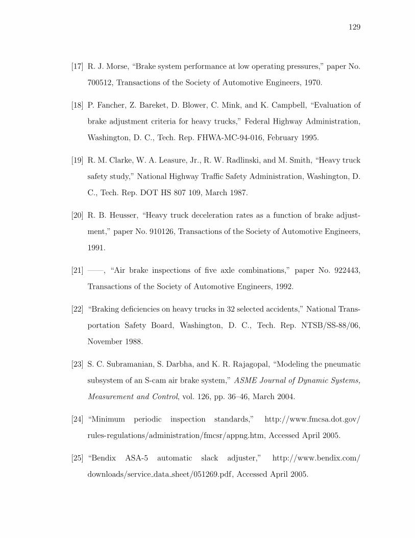
129

[17] R. J. Morse, “Brake system performance at low operating pressures,” paper No.


[18] P. Fancher, Z. Bareket, D. Blower, C. Mink, and K. Campbell, “Evaluation of

brake adjustment criteria for heavy trucks,” Federal Highway Administration,

Washington, D. C., Tech. Rep. FHWA-MC-94-016, February 1995.

[19] R. M. Clarke, W. A. Leasure, Jr., R. W. Radlinski, and M. Smith, “Heavy truck

safety study,” National Highway Traffic Safety Administration, Washington, D.

C., Tech. Rep. DOT HS 807 109, March 1987.

[20] R. B. Heusser, “Heavy truck deceleration rates as a function of brake adjust-

ment,” paper No. 910126, Transactions of the Society of Automotive Engineers,

1991.

[21] ——, “Air brake inspections of five axle combinations,” paper No. 922443,

Transactions of the Society of Automotive Engineers, 1992.

[22] “Braking deficiencies on heavy trucks in 32 selected accidents,” National Trans-

portation Safety Board, Washington, D. C., Tech. Rep. NTSB/SS-88/06,

November 1988.

[23] S. C. Subramanian, S. Darbha, and K. R. Rajagopal, “Modeling the pneumatic

subsystem of an S-cam air brake system,” ASME Journal of Dynamic Systems,

Measurement and Control, vol. 126, pp. 36–46, March 2004.

[24] “Minimum periodic inspection standards,” http://www.fmcsa.dot.gov/

rules-regulations/administration/fmcsr/appng.htm, Accessed April 2005.

[25] “Bendix ASA-5 automatic slack adjuster,” http://www.bendix.com/

downloads/service data sheet/051269.pdf, Accessed April 2005.

130

[26] D. Middleton and J. Rowe, “Feasibility of standardized diagnostic device for

maintenance and inspection of commercial motor vehicles,” Transportation Re-

search Record, vol. 1560, pp. 48–56, 1996.

[27] E. Zaloshnja and T. Miller, “Revised costs of large truck-and bus-involved

crashes,” Federal Motor Carrier Safety Administration, Washington, D. C.,

Tech. Rep., November 2002.

[28] “Commodity flow survey,” 1997 Economic Census, U. S. Census Bureau, 1997.

[29] A. Barber, Pneumatic Handbook, 8th ed. Oxford, United Kingdom: Elsevier

Advanced Technology, 1997.

[30] W. H. Kruse, Jr., “The history and development of railroad braking,” B.S.

Thesis, University of Cincinnati, 1948.

[31] W. V. Turner, The Air Brake as Related to Progress in Locomotion. Pittsburg,

Pennsylvania: Westinghouse Air Brake Company, 1910.

[32] F. H. Wells, “The development of the modern air brake,” M.E. Thesis, Mas-

sachussetts Institute of Technology, 1920.

[33] H. G. Prout, A Life of George Westinghouse. New York: The American Society

of Mechanical Engineers, 1921.

[34] F. E. Leupp, George Westinghouse: His Life and Achievements. Boston: Little,

Brown, and Company, 1918.

[35] P. Synnestvedt, Evolution of the Air Brake. New York: Locomotive Engineer-

ing, 1895.

131

[36] ——, Diseases of the Air Brake System: Their Causes, Symptoms and Cures.

Chicago: The W. F. Hall Printing Company, 1896.

[37] G. A. Harper, Brakes and Friction Materials: The History and Development of

the Technologies. London, UK: Mechanical Engineering Publications Limited,

1998.

[38] D. G. Blaine, Modern Freight Car Air Brakes. Omaha, Nebraska: Simmons-

Boardman Publishing Corporation, 1979.

[39] L. C. Buckman, “Commercial vehicle braking systems: Air brakes, ABS and

beyond,” Society of Automotive Engineers, Indianapolis, the 43rd L. Ray Buck-

endale Lecture, International Truck and Bus Meeting and Exposition, Indi-

anapolis, Society of Automotive Engineers, November, 1998.

[40] “Heavy vehicle airbrake performance,” National Transportation Safety Board,

Washington, D. C., Tech. Rep. NTSB/SS-92/01, April 1992.

[41] S. Tanaka, K. Kubota, T. Iwasaki, and H. Hatanaka, “The compatibility of

air disc brakes and S-cam brakes installed on combination vehicles,” paper No.


[42] E. Gohring and E. C. Von Glasner, “Performance comparison of drum and disc

brakes for heavy duty commercial vehicles,” paper No. 902206, Transactions of

the Society of Automotive Engineers, 1990.

[43] A. C. Esteves, L. Winocq, and J. Berthaud, “Disc brakes for trucks: A technical

innovation for heavy vehicles,” paper No. 925059, Transactions of the Society

of Automotive Engineers, 1992.

132

[44] W. A. Leasure, Jr. and S. F. Williams, Jr., “Antilock systems for air-braked ve-

hicles,” paper No. 890113, The Thirty-Fifth L. Ray Buckendale Lecture, Trans-

actions of the Society of Automotive Engineers, 1989.

[45] G. P. Mathews, “Art and science of braking heavy duty vehicles,” paper No.

640795, The Tenth L. Ray Buckendale Lecture, Transactions of the Society of

Automotive Engineers, 1964.

[46] D. Kramer, D. Roper, and E. Trachman, “Drive axle antilock for heavy ve-

hicle stability,” paper No. 871572, Transactions of the Society of Automotive

Engineers, 1987.

[47] P. Berg, Compressed-Air Systems for Commercial Vehicles: 1 - Basic Princi-

ples, Systems and Schematic Diagrams, 3rd ed. Stuttgart, Germany: Robert

Bosch, 1999.

[48] E. Peterson, E. Reinecke, and P. Liermann, “Anti-lock braking systems (ABS)

with integrated drive slip control (ASR) for commercial vehicles,” paper No.


[49] H. Decker and J. Wrede, “Brake-by-wire: Solutions, advantages and the need for

standardization,” paper No. 94C039, Transactions of the Society of Automotive

Engineers, 1994.

[50] C. Wiehen and D. Neuhaus, “Potential of electronically controlled brake sys-

tems,” paper No. 952278, Transactions of the Society of Automotive Engineers,

1995.

[51] K. Linderman, E. Peterson, M. Schult, and A. Korn, “EBS and tractor trailer

133

brake compatibility,” paper No. 973283, Transactions of the Society of Auto-

motive Engineers, 1997.

[52] J. E. Fent, “U.S.A. commercial vehicle air brake systems – 1991 overview,”

paper No. 918013, Transactions of the Society of Automotive Engineers, 1991.

[53] “Front wheel brake safety facts,” Department of Transportation, Federal High-

way Administration, Washington, D. C., 1987.

[54] “EC series electric cylinders: User’s manual,” PN CUS10050, Version 1.0, In-

dustrial Devices Corporation/Danaher Motion, Rockford, Illinois.

[55] “B8501: Brushless analog position control manual supplement,” PN PCW-4712,

Rev. 1.01, Industrial Devices Corporation/Danaher Motion, Rockford, Illinois,

June 1995.

[56] “B8001 brushless servo drive: Operator’s manual,” PN PCW-4679, Rev. 1.5,

Industrial Devices Corporation/Danaher Motion, Rockford, Illinois, May 1998.

[57] “IDC Servo Tuner: Operator’s manual,” P/N PCW-4710, Rev. 1.00, Industrial

Devices Corporation/Danaher Motion, Rockford, Illinois, April 1995.

[58] J. Tal, Step-by-Step Design of Motion Control Systems. Sunnyvale, California:

Galil Motion Control, Inc., 1994.

[59] “PCI E series user manual: Multifunction I/O devices for PCI bus computers,”

National Instruments, Austin, Texas, July 2002.

[60] G. W. Johnson and R. Jennings, Labview Graphical Programming, 3rd ed. New

York: McGraw-Hill, 2001.

134

[61] J. C. Gerdes and J. K. Hedrick, “Brake system modeling for simulation and

control,” ASME Journal of Dynamic Systems, Measurement and Control, vol.

121, pp. 496–503, September 1999.

[62] Y. Khan, P. Kulkarni, and K. Youcef-Toumi, “Modeling, experimentation and

simulation of a brake apply system,” ASME Journal of Dynamic Systems, Mea-

surement and Control, vol. 116, pp. 111–122, March 1994.

[63] D. K. Fisher, “Brake system component dynamic performance measurement

and analysis,” paper No. 700373, Transactions of the Society of Automotive

Engineers, 1970.

[64] L. Johnson, P. S. Fancher, and T. D. Gillespie, “An empirical model for the

prediction of the torque output of commercial vehicle air brakes,” Highway

Safety Research Institute, University of Michigan, Ann Arbor, Michigan, Tech.

Rep. UM-HSRI-78-53, December 1978.

[65] T. M. Post, P. S. Fancher, and J. E. Bernard, “Torque characteristics of com-

mercial vehicle brakes,” paper No. 750210, Transactions of the Society of Au-

tomotive Engineers, 1975.

[66] P. G. Reinhall and R. R. Scheibe, “Development of an intelligent air brake warn-

ing system for commercial vehicles,” IDEA Program, Transportation Research

Board, National Research Council, Washington, D. C., Tech. Rep. ITS-13, May

1996.

[67] T. Acarman, U. Ozguner, C. Hatipoglu, and A. M. Igusky, “Pneumatic brake

system modeling for systems analysis,” paper No. 2000-01-3414, Transactions

of the Society of Automotive Engineers, 2000.

135

[68] A. L. Dunn, G. J. Heydinger, G. Rizzoni, and D. A. Guenther, “New model

for simulating the dynamics of pneumatic heavy truck brakes with integrated

anti-lock control,” paper No. 2003-01-1322, Transactions of the Society of Au-

tomotive Engineers, 2003.

[69] L. D. Kandt, P. G. Reinhall, and R. R. Scheibe, “Determination of air brake

adjustment from air pressure data,” Proc. Institution of Mechanical Engineers,

Part D: Journal of Automobile Engineering, vol. 215, pp. 21–29, 2001.

[70] B. W. Anderson, The Analysis and Design of Pneumatic Systems. New York:

John Wiley & Sons, Inc., 1967.

[71] H. E. Merritt, Hydraulic Control Systems. New York: John Wiley & Sons,

1967.

[72] W. Bolton, Pneumatic and Hydraulic Systems. Oxford, England: Butterworth-

Heinemann, 1997.

[73] A. Balluchi, L. Benvenuti, M. D. Di Benedetto, C. Pinello, and A. L.

Sangiovanni-Vincentelli, “Automotive engine control and hybrid systems: Chal-

lenges and opportunities,” Proc. IEEE, vol. 88, no. 7, pp. 888–912, 2000.

[74] F. Borrelli, A. Bemporad, M. Fodor, and D. Hrovat, “A hybrid control approach

to traction control,” in Hybrid Systems: Computation and Control, ser. Lecture

Notes in Computer Science, M. D. Di Benedetto and A. Sangiovanni-Vincentelli,

Eds., vol. 2034. Berlin, Germany: Springer-Verlag, 2001, pp. 162–174.

[75] C. Altafini, A. Speranzon, and K. H. Johansson, “Hybrid control of a truck

and trailer vehicle,” in Hybrid Systems: Computation and Control, ser. Lecture

136

Notes in Computer Science, C. J. Tomlin and M. R. Greenstreet, Eds., vol.

2289. Berlin, Germany: Springer-Verlag, 2002, pp. 21–34.

[76] A. Balluchi, L. Benvenuti, M. D. Di Benedetto, and A. L. Sangiovanni-

Vincentelli, “A hybrid observer for the driveline dynamics,” in Proc. European

Control Conference, Porto, Portugal, 2001, pp. 618–623.

[77] S. J. Sobolak, “Simulation of the Ford vehicle speed control system,” paper No.


[78] P. G. Blaney, “Improvements to cruise controls utilizing microprocessor technol-

ogy,” paper No. 830662, Transactions of the Society of Automotive Engineers,

1983.

[79] Y. Harada, H. Miyata, Y. Hayakawa, and S. Fujii, “Cruise control system us-

ing adaptive control theory,” paper No. 931917, Transactions of the Society of

Automotive Engineers, 1993.

[80] P. Martin, “Autonomous intelligent cruise control incorporating automatic

braking,” paper No. 930510, Transactions of the Society of Automotive En-

gineers, 1993.

[81] D. Wuh, “Design and comparison of autonomous intelligent cruise control sys-

tems,” paper No. 942405, Transactions of the Society of Automotive Engineers,

1994.

[82] P. Francher, Z. Bareket, S. Bogard, C. MacAdam, and R. Ervin, “Tests charac-

terizing performance of an adaptive cruise control system,” paper No. 970458,

Transactions of the Society of Automotive Engineers, 1997.

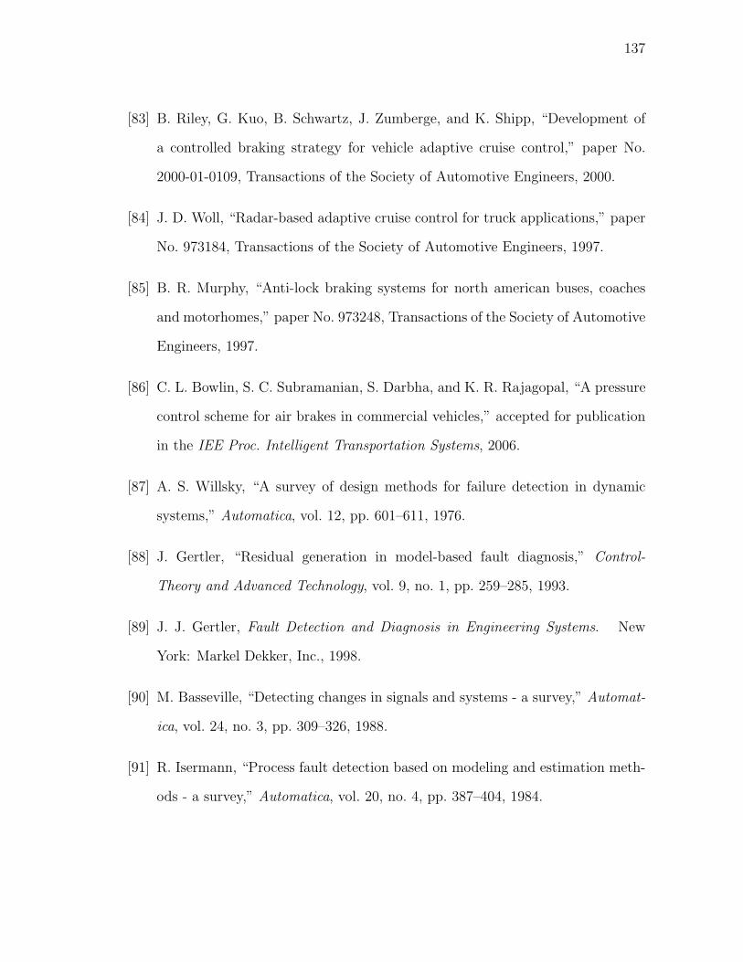
137

[83] B. Riley, G. Kuo, B. Schwartz, J. Zumberge, and K. Shipp, “Development of

a controlled braking strategy for vehicle adaptive cruise control,” paper No.

2000-01-0109, Transactions of the Society of Automotive Engineers, 2000.

[84] J. D. Woll, “Radar-based adaptive cruise control for truck applications,” paper

No. 973184, Transactions of the Society of Automotive Engineers, 1997.

[85] B. R. Murphy, “Anti-lock braking systems for north american buses, coaches

and motorhomes,” paper No. 973248, Transactions of the Society of Automotive

Engineers, 1997.

[86] C. L. Bowlin, S. C. Subramanian, S. Darbha, and K. R. Rajagopal, “A pressure

control scheme for air brakes in commercial vehicles,” accepted for publication

in the IEE Proc. Intelligent Transportation Systems, 2006.

[87] A. S. Willsky, “A survey of design methods for failure detection in dynamic

systems,” Automatica, vol. 12, pp. 601–611, 1976.

[88] J. Gertler, “Residual generation in model-based fault diagnosis,” Control-

Theory and Advanced Technology, vol. 9, no. 1, pp. 259–285, 1993.

[89] J. J. Gertler, Fault Detection and Diagnosis in Engineering Systems. New

York: Markel Dekker, Inc., 1998.

[90] M. Basseville, “Detecting changes in signals and systems - a survey,” Automat-

ica, vol. 24, no. 3, pp. 309–326, 1988.

[91] R. Isermann, “Process fault detection based on modeling and estimation meth-

ods - a survey,” Automatica, vol. 20, no. 4, pp. 387–404, 1984.

138

[92] P. M. Frank, “Fault diagnosis in dynamic systems using analytical and

knowledge-based redundancy - a survey and some new results,” Automatica,

vol. 26, no. 3, pp. 459–474, 1990.

[93] “FMCSA rule for PBBTs,” http://www.dot.gov/affairs/fmcsa1502.htm, Ac-

cessed August 2004.

[94] “US patents,” http://www.uspto.gov, Accessed August 2004.

[95] “Personal communication,” personal communication with Professor Pravin

Varaiya, 2004.

[96] “Bendix brake chambers,” http://www.bendix.com/downloads/service data

sheet/021302.pdf, Accessed April 2005.

[97] J. J. E. Slotine and W. Li, Applied Nonlinear Control. Englewood Cliffs, New

Jersey: Prentice Hall, 1991.

[98] S. Sastry and M. Bodson, Adaptive Control: Stability, Convergence and Ro-

bustness. Englewood Cliffs, New Jersey: Prentice Hall, 1989.

[99] D. Liberzon and A. S. Morse, “Basic problems in stability and design of switched

systems,” IEEE Control Systems Magazine, vol. 19, no. 5, pp. 59–70, October

1999.

[100] A. Alessandri and P. Coletta, “Design of Luenberger observers for a class of hy-

brid linear systems,” in Hybrid Systems: Computation and Control, ser. Lecture

Notes in Computer Science, M. D. D. Benedetto and A. Sangiovanni-Vincentelli,

Eds., vol. 2034. Berlin, Germany: Springer-Verlag, 2001, pp. 7–18.

[101] R. Vidal, A. Chiuso, S. Soatto, and S. Sastry, “Observability of linear hybrid

systems,” in Hybrid Systems: Computation and Control, ser. Lecture Notes in

139

Computer Science, O. Maler and A. Pnueli, Eds., vol. 2623. Berlin, Germany:

Springer-Verlag, 2003, pp. 526–539.

[102] J. P. Hespanha and A. S. Morse, “Switching between stabilizing controllers,”

Automatica, vol. 38, pp. 1905–1917, 2002.

[103] D. Swaroop and K. R. Rajagopal, “Limit of a collection of dynamical systems:

An application to modeling the dynamics of flow of traffic,” Mathematical Mod-

els and Methods in Applied Sciences, vol. 12, no. 10, pp. 1381–1399, 2002.

[104] R. W. Radlinski and M. A. Flick, “Tractor and trailer brake system compatibil-

ity,” paper No. 861942, Transactions of the Society of Automotive Engineers,

1986.

140

VITA

Shankar Ram Coimbatore Subramanian was born in the south Indian state of

Tamilnadu. He was brought up in the city of Chennai and completed high school there.

He obtained his Bachelor of Engineering in mechanical engineering from the University

of Allahabad, Allahabad, India, in May 2000. He joined the Department of Mechanical

Engineering at Texas A&M University in August 2000 to pursue his Master of Science in

mechanical engineering and graduated with the same in May 2003. Then, he continued

pursuing his Ph.D. in mechanical engineering at Texas A&M University and graduated

with the same in May 2006. He may be contacted through Professor K. R. Rajagopal,

Department of Mechanical Engineering, Texas A&M University, College Station, Texas

77843, USA.

The typist for this dissertation was Shankar Ram Coimbatore Subramanian.

Documents

A Diagnostic System for Air Brakes in Commercial Vehicles (PDF