Embed Size (px)
Citation preview
1
A DETAILED VIEW ON THE MIXING AND LOSS GENERATION
PROCESS DURING STEAM ADMISSION CONCERNING
GEOMETRY, TEMPERATURE AND PRESSURE
D. Engelmann – R. Mailach
Ruhr-Universität Bochum, Chair of Thermal Turbomachinery, 44780, Bochum, Germany,
ABSTRACT
Steam turbines used in industrial applications often contain several branches for the
admission of steam. Those branches are placed at the axial connections of two stage groups or
within a single module. Among geometrical parameters, different temperature and pressure
levels have a great impact on the mixing process of main and branch mass flows and on the
flow distribution in subsequent turbine stages. Therefore, it is essential to understand the loss
mechanisms appearing at junctions of different mass flow partitions to guarantee a stable
operation and a high efficiency in a wide range of steam load.
A comprehensive parameterized numerical study of a generic steam admission junction is
described in this paper which focusses on geometry dependencies as well as on temperature
and pressure differences. The study is performed with a 3D RANS solver to determine several
loss partitions, such as total pressure loss, wall friction and admission loss. The results of the
flow simulations are compared to literature values and empirical loss assumptions with a
detailed view on both main steam path and branch pipe.
NOMENCLATURE
INTRODUCTION
Modern steam turbines are not only used for electric power generation in fossil power plants but
rather satisfy a wide range of industrial applications. They can be found in the process of Fluid
Catalytic Cracking (FCC) or Carbon Dioxide Capture and Storage (CCS). They are furthermore
utilized in captive power plants e.g. for paper mills, mining, food production, the chemical industry
A m² area
a m width of main channel
AR % area ratio, b/a
b m width of branch channel
FR % flow ratio, OutBr mm
m kg/s mass flow
P m Perimeter
p Pa pressure
T °C temperature
TR % transition radius related to
outlet diameter
Greek Symbols
ζ - pressure loss coefficient
τW N/m² wall shear stress
Subscripts
adm admission
CS cross sectional
fr friction
In inlet
Out outlet
Br branch
Sf surface
t total
W wall
Abbreviations
K kink
v vapour
w water
Proceedings of
11th European Conference on Turbomachinery Fluid dynamics & Thermodynamics
ETC11, March 23-27, 2015, Madrid, Spain
OPEN ACCESS
Downloaded from www.euroturbo.eu Copyright © by the Authors

2
or applied in Concentrated Solar Power plants (CSP) and within Combined Heat and Power (CHP).
This huge field of applications with its diverse demands requires a flexible, modular and compact
design of industrial steam turbines. Therefore, the control stage as well as several interchangeable
high, intermediate and low pressure modules are combined together within a single turbine casing.
In contrast to common power plant turbines, they feature a high and also variable rotational speed
up to 18,000 RPM with an output range of a few kilowatt to a maximum value of today 200 MW.
Usually, an industrial steam turbine includes several branches which are placed at the axial
connections of two stage groups or within a single module. Steam admission through these branches
can have a serious impact on the operational behaviour of a steam turbine. When the branch mass
flow joins the main steam path flow an additional secondary pressure loss occurs which is caused
by the deflection and the inhomogeneous mixing process of the admitted steam with main flow
partitions. The amount of loss depends on rotational speed, junction geometry and steam parameters
such as degree of admission, pressure level and temperature. Therefore, it is important to estimate
the loss mechanisms appearing at these junctions to enable a high efficiency together with a stable
operation despite the variation in the steam load.
In literature several loss mechanisms are described for the main flow path of gas and steam
turbines with shrouded blades. Denton (1993) e.g. provided formulations for the estimation of
losses which are caused by the interaction of the re-entering shroud cavity flow with the blade
channel flow. Some more loss mechanisms are given by Wallis et al. (2000) which studied turning
device configurations in order to reduce shroud cavity losses in a four stage axial turbine. They
reported four types of losses concerning labyrinth seals, counter rotating cavity walls, flow mixing
at the cavity outlet and subsequent stages. Gier et al. (2003) applied these given loss definitions to a
numerical investigation of a three stage low pressure turbine for jet engines and added another loss
mechanism which is caused by steps at the sidewalls of the flow path.
A lack of information exists regarding the influence of turning, mixing and separation of branch
mass flow partitions and its related additional secondary pressure loss or in other words admission
loss. The reason behind this are missing experimental results, which are connected one the one side
with a compact steam turbines design and on the other side with adverse fluid conditions. Thick-
walled, pressure-stable casings and guide vane carriers hamper the local accessibility for
measurement probes or optical systems. Moreover, water-vapour raises the demands for
measurement equipment. Condensate can block sensor heads or wall pressure taps and thereby
falsify the experimental output.
By now, the most convenient data in the open literature is given by Idelchik (1986) and Miller
(1990). They collected pressure loss data for fluid flow through pipes and specific components such
as sudden openings, valves, manifolds, nozzles and flow junctions while some new attempts deal
with the estimation of pressure losses for turbine blade coolant flows. Barringer et al. (2014) for
example provide numerical and experimental data for static pressure losses of inlet and exit holes in
a generic up-scaled coolant channel with air at ambient conditions.
Numerical studies for T-junctions with circular pipes were performed by Walker et al. (2010).
They adjusted the parameters of several common RANS turbulence models to improve the
prediction of the downstream flow mixing. Kuczay et al. (2010), on the other hand, used LES
simulations to gain more insights of the thermal mixing downstream the junction. Both publications
relate to experiments of Andersson et al. (2006) who investigated the flow mixing in a pipe-junction
with a temperature difference of 15 K between inlet and branch pipe. However, all mentioned
sources neither directly refer to admission in steam turbines nor use vapour as fluid in combination
with a high pressure and temperature level. Likewise, prediction of admission in steam turbines is
sophisticated due to asymmetrical inflow and inhomogeneous flow mixing which cause a complex
3D flow field and concomitant a high numerical effort.
With the aim to gain more information about admission losses in industrial steam turbines
several numerical studies with a generic T-junction were performed in the recent past. Therefore, in
the first part of this publication a brief summary of past research activities is given. This concerns
3
geometry details, loss calculation method, fluid parameters as well as achieved results which are
partially already published. Whilst the past investigations solely focus on loss values for the main
steam path, a detailed view on both main steam path and branch pipe is given here. The second part
deals with temperature and pressure differences at the inlet of main path and branch pipe and their
effects on the mixing and loss generation process.
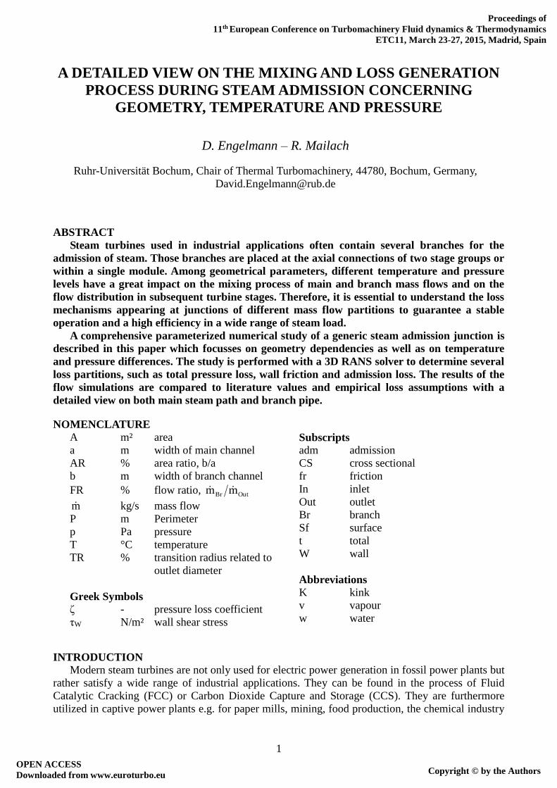
T-JUNCTION GEOMETRY AND SIMULATION PROCEDURE
Several issues arise if one attempt to use admission loss values from the literature for steam
turbines. Experimental data given by Idelchik (1986) and Miller (1990) are based on flow through
pipe junctions with water at ambient condition (see Figure 1, left).
TR TR TR
TR + a
TR TR
a
Figure 1: Comparison of pipe junctions with rounded transitions; Left: circular pipe junction (Miller
(1990); Middle: rectangular pipe junction with beneficial flow guide (Idelchik (1986); Right:
generic T-junction for parameterized numerical study
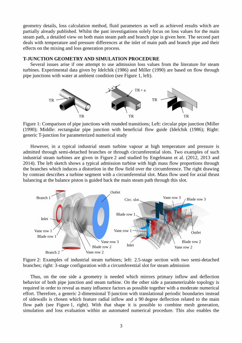
However, in a typical industrial steam turbine vapour at high temperature and pressure is
admitted through semi-detached branches or through circumferential slots. Two examples of such
industrial steam turbines are given in Figure 2 and studied by Engelmann et al. (2012, 2013 and
2014). The left sketch shows a typical admission turbine with high mass flow proportions through
the branches which induces a distortion in the flow field over the circumference. The right drawing
by contrast describes a turbine segment with a circumferential slot. Mass flow used for axial thrust
balancing at the balance piston is guided back the main steam path through this slot.
Inlet
Outlet
Branch 2
Branch 1
Vane row 1
Blade row 2
Vane row 2
Blade row 1
Vane row 3Inlet
Outlet
Circ. slot
Vane row 1
Blade row 1
Vane row 2
Blade row 2
Vane row 3 Blade row 3
Figure 2: Examples of industrial steam turbines; left: 2.5-stage section with two semi-detached
branches; right: 3-stage configuration with a circumferential slot for steam admission
Thus, on the one side a geometry is needed which mirrors primary inflow and deflection
behavior of both pipe junction and steam turbine. On the other side a parameterizable topology is
required in order to reveal as many influence factors as possible together with a moderate numerical
effort. Therefore, a generic 2-dimensional T-junction with translational periodic boundaries instead
of sidewalls is chosen which feature radial inflow and a 90 degree deflection related to the main
flow path (see Figure 1, right). With that shape it is possible to combine mesh generation,
simulation and loss evaluation within an automated numerical procedure. This also enables the
4
calculation of loss values for a huge combination of mass flows, area ratios, and transition radii as
well as for several turbulence models and fluid properties.
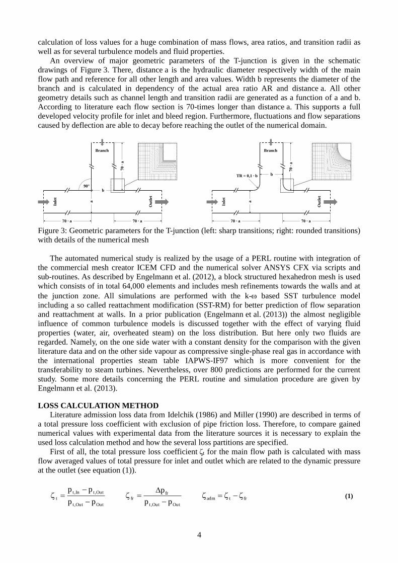
An overview of major geometric parameters of the T-junction is given in the schematic
drawings of Figure 3. There, distance a is the hydraulic diameter respectively width of the main
flow path and reference for all other length and area values. Width b represents the diameter of the
branch and is calculated in dependency of the actual area ratio AR and distance a. All other
geometry details such as channel length and transition radii are generated as a function of a and b.
According to literature each flow section is 70-times longer than distance a. This supports a full
developed velocity profile for inlet and bleed region. Furthermore, fluctuations and flow separations
caused by deflection are able to decay before reaching the outlet of the numerical domain.
a
b90°
Branch
Inle
t
Ou
tlet
70 ∙ a 70 ∙ a
70
∙ a
a
b
Branch
Inle
t
Ou
tlet
TR = 0,1 ∙ b
70 ∙ a70 ∙ a
70
∙ a
Figure 3: Geometric parameters for the T-junction (left: sharp transitions; right: rounded transitions)
with details of the numerical mesh
The automated numerical study is realized by the usage of a PERL routine with integration of
the commercial mesh creator ICEM CFD and the numerical solver ANSYS CFX via scripts and
sub-routines. As described by Engelmann et al. (2012), a block structured hexahedron mesh is used
which consists of in total 64,000 elements and includes mesh refinements towards the walls and at
the junction zone. All simulations are performed with the k- based SST turbulence model
including a so called reattachment modification (SST-RM) for better prediction of flow separation
and reattachment at walls. In a prior publication (Engelmann et al. (2013)) the almost negligible
influence of common turbulence models is discussed together with the effect of varying fluid
properties (water, air, overheated steam) on the loss distribution. But here only two fluids are
regarded. Namely, on the one side water with a constant density for the comparison with the given
literature data and on the other side vapour as compressive single-phase real gas in accordance with
the international properties steam table IAPWS-IF97 which is more convenient for the
transferability to steam turbines. Nevertheless, over 800 predictions are performed for the current
study. Some more details concerning the PERL routine and simulation procedure are given by
Engelmann et al. (2013).
LOSS CALCULATION METHOD
Literature admission loss data from Idelchik (1986) and Miller (1990) are described in terms of
a total pressure loss coefficient with exclusion of pipe friction loss. Therefore, to compare gained
numerical values with experimental data from the literature sources it is necessary to explain the
used loss calculation method and how the several loss partitions are specified.
First of all, the total pressure loss coefficient ζt for the main flow path is calculated with mass
flow averaged values of total pressure for inlet and outlet which are related to the dynamic pressure
at the outlet (see equation (1)).
OutOut,t
Out,tIn,t
tpp
pp
OutOut,t
frfr
pp
p
frtadm (1)
5
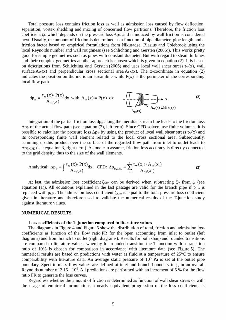
Total pressure loss contains friction loss as well as admission loss caused by flow deflection,
separation, vortex shedding and mixing of concerned flow partitions. Therefore, the friction loss
coefficient ζfr which depends on the pressure loss Δpfr and is induced by wall friction is considered
next. Usually, the amount of friction is determined as a function of pipe diameter, pipe length and a
friction factor based on empirical formulations from Nikuradse, Blasius and Colebrook using the
local Reynolds number and wall roughness (see Schlichting and Gersten (2006)). This works pretty
good for simple geometries such as pipes with constant diameter. But with regard to steam turbines
and their complex geometries another approach is chosen which is given in equation (2). It is based
on descriptions from Schlichting and Gersten (2006) and uses local wall shear stress τw(x), wall
surface AW(x) and perpendicular cross sectional area ACS(x). The x-coordinate in equation (2)
indicates the position on the meridian streamline while P(x) is the perimeter of the corresponding
local flow path.
Integration of the partial friction loss dpfr along the meridian stream line leads to the friction loss
Δpfr of the actual flow path (see equation (3), left term). Since CFD solvers use finite volumes, it is
possible to calculate the pressure loss Δpfr by using the product of local wall shear stress τw(x) and
its corresponding finite wall element related to the local cross sectional area. Subsequently,
summing up this product over the surface of the regarded flow path from inlet to outlet leads to
Δpfr,CFD (see equation 3, right term). As one can assume, friction loss accuracy is directly connected
to the grid density, thus to the size of the wall elements.
Analytical: dx)x(A
)x(P)x(p
CS
Wfr
CFD:
n
1i iCS
iWiWCFD,fr
)x(A
)x(A)x(p
At last, the admission loss coefficient ζadm can be derived when subtracting ζfr from ζt (see
equation (1)). All equations explained in the last passage are valid for the branch pipe if pt,In is
replaced with pt,Br. The admission loss coefficient ζadm is equal to the total pressure loss coefficient
given in literature and therefore used to validate the numerical results of the T-junction study
against literature values.
NUMERICAL RESULTS
Loss coefficients of the T-junction compared to literature values
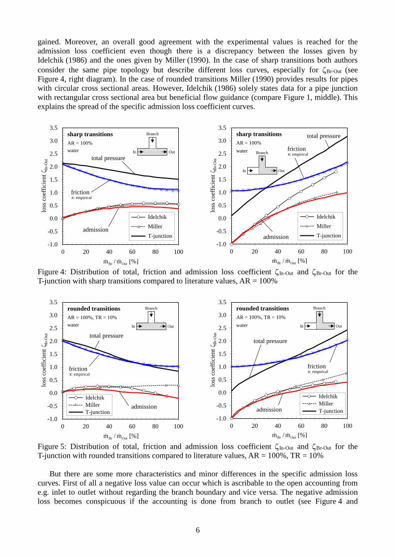
The diagrams in Figure 4 and Figure 5 show the distribution of total, friction and admission loss
coefficients as function of the flow ratio FR for the open accounting from inlet to outlet (left
diagrams) and from branch to outlet (right diagrams). Results for both sharp and rounded transitions
are compared to literature values, whereby for rounded transition the T-junction with a transition
ratio of 10% is chosen for comparison in accordance with literature data (see Figure 5). The
numerical results are based on predictions with water as fluid at a temperature of 25°C to ensure
comparability with literature data. An average static pressure of 105 Pa is set at the outlet pipe
boundary. Specific mass flow values are defined at inlet and branch boundary to gain an overall
Reynolds number of 2.15 · 105. All predictions are performed with an increment of 5 % for the flow
ratio FR to generate the loss curves.
Regardless whether the amount of friction is determined as function of wall shear stress or with
the usage of empirical formulations a nearly equivalent progression of the loss coefficients is
dx
)x(A
)x(P)x(dp
CS
Wfr
with dx)x(P)x(AW
ACS(x)AW(x) with τw(x)
x
ACS(x)AW(x) with τw(x)
x
(2)
(3)
6
gained. Moreover, an overall good agreement with the experimental values is reached for the
admission loss coefficient even though there is a discrepancy between the losses given by
Idelchik (1986) and the ones given by Miller (1990). In the case of sharp transitions both authors
consider the same pipe topology but describe different loss curves, especially for Br-Out (see
Figure 4, right diagram). In the case of rounded transitions Miller (1990) provides results for pipes
with circular cross sectional areas. However, Idelchik (1986) solely states data for a pipe junction
with rectangular cross sectional area but beneficial flow guidance (compare Figure 1, middle). This
explains the spread of the specific admission loss coefficient curves.
[%]m/m OutBr
loss
coef
fici
ent
ζ In
-Ou
t
-1.0
-0.5
0.0
0.5
1.0
1.5
2.0
2.5
3.0
3.5
0 20 40 60 80 100
Idelchik
Miller
T-junction
Total
Friction
Seconary
Kurven für A=100% und M in 5% Schritte
total pressure
friction
admission
sharp transitions
In Out
Branch
x: empirical
AR = 100%
water
[%]m/m OutBr
loss
coef
fici
ent
ζ Br-
Ou
t
-1.0
-0.5
0.0
0.5
1.0
1.5
2.0
2.5
3.0
3.5
0 20 40 60 80 100
Idelchik
Miller
T-junction
Kurven für A=100% und M in 5% Schritte
total pressure
admission
sharp transitions
frictionx: empirical
In Out
Branch
AR = 100%
water
Figure 4: Distribution of total, friction and admission loss coefficient In-Out and Br-Out for the
T-junction with sharp transitions compared to literature values, AR = 100%
[%]m/m OutBr
-1.0
-0.5
0.0
0.5
1.0
1.5
2.0
2.5
3.0
3.5
0 20 40 60 80 100
Idelchik
Miller
T-junction
Total
Friction
Seconary
Kurven für A=100% und M in 5% Schritte
loss
coef
fici
ent
ζ In
-Ou
t
total pressure
admission
rounded transitions
In Out
Branch
frictionx: empirical
AR = 100%, TR = 10%
water
[%]m/m OutBr
loss
coef
fici
ent
ζ Br-
Ou
t
-1.0
-0.5
0.0
0.5
1.0
1.5
2.0
2.5
3.0
3.5
0 20 40 60 80 100
Idelchik
Miller
T-junction
Kurven für A=100% und M in 5% Schritte
total pressure
admission
rounded transitions
frictionx: empirical
In Out
Branch
AR = 100%, TR = 10%
water
Figure 5: Distribution of total, friction and admission loss coefficient In-Out and Br-Out for the
T-junction with rounded transitions compared to literature values, AR = 100%, TR = 10%
But there are some more characteristics and minor differences in the specific admission loss
curves. First of all a negative loss value can occur which is ascribable to the open accounting from
e.g. inlet to outlet without regarding the branch boundary and vice versa. The negative admission
loss becomes conspicuous if the accounting is done from branch to outlet (see Figure 4 and
7
Figure 5, right diagrams). For a zero flow ratio FR the whole mass flow is contributed by the inlet
channel. In this case, total and static pressure in the branch channel as well as static pressure within
the junction zone show almost the same values. Due to the inlet mass flow with its high velocity,
total pressure is higher than static pressure within the junction zone. This leads to a rapid rise of the
branch total pressure when reaching the junction zone which then in turn is decreased in the outlet
channel mainly because of the friction loss. As the curves in the right diagrams of Figure 4 and
Figure 5 illustrate, there is only a small pt, Br-Out and therefore t, Br-Out. As opposed to this,
pfr, Br-Out and therefore fr, Br-Out are much higher because they are mainly driven by the high
velocity of the inlet mass flow.
When looking at In-Out, there is a small but already existing amount of admission loss for a
flow ratio FR = 0%. The reason for this can be found in fluid partitions coming from the inlet
channel which enter and circulate inside the branch channel when crossing it. Unfortunately, this
effect is not considered in the literature for the accounting from inlet to outlet (see Figure 5, left).
Furthermore, increasing the branch flow leads to a minor under-prediction of the numerical loss
coefficients. This effect is attributable to the absence of sidewalls for the T-junction (see Figure 1).
Similar to the flow behaviour in a 90°-manifold and due to deflection of the branch flow a pressure
gradient between inner and outer bend arises. As a result of side wall friction in pipe junctions with
circular or rectangular cross sectional area, a cross flow perpendicular to the main flow is formed to
counterbalance this pressure gradient. Interaction of the cross flow with the main flow then leads to
a higher secondary loss coefficient. In contrast to this, the pipes of the flat T-junction do not have
sidewalls which means a comparable cross flow does not arise. Finally, rounded transitions lead to
reduced admission loss values compared to sharp transitions. This can be explained with better flow
guidance, a later separation of the deflected branch flow (compare the several kinks K1 to K4 in
Figure 6 and Figure 7) and a smaller separation zone as mentioned by Engelmann et al. (2014).
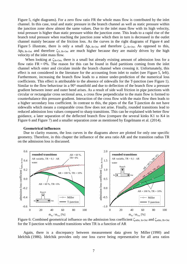
Geometrical influences
Due to clarity reasons, the loss curves in the diagrams above are plotted for only one specific
geometry. Therefore, in this chapter the influence of the area ratio AR and the transition radius TR
on the admission loss is discussed.
adm
issi
on
loss
coef
fici
ent
ζ ad
m, In
-Ou
t
-0.6
-0.4
-0.2
0.0
0.2
0.4
0.6
0 20 40 60 80 100
Miller
T-junction
Kurven für A=50 bis 100% in 10% und M in 5% Schritte
R_Fillet = 10% vom Hydr. Durchmesser des Zweigs
AR = 60 %,
TR= 6%
AR = 100 %, TR = 10%
AR variable, TR = 0,1 ∙ AR
[%]m/m OutBr
rounded transitions
In Out
Branch
AR = 60 %, TR= 6%
water
AR variable, TR = 0,1 ∙ AR
adm
issi
on
loss
coef
fici
ent
ζ ad
m, B
r-O
ut
[%]m/m OutBr
rounded transitions
In Out
Branch
AR = 100 %, TR = 10%
-1.0
-0.5
0.0
0.5
1.0
1.5
2.0
0 20 40 60 80 100
Miller
T-junction
Kurven für A=100% bis 50% mit R5 bis R2,5mm und M in 5% Schritte
water
Figure 6: Combined geometrical influence on the admission loss coefficient adm, In-Out and adm, Br-Out
for the T-junction with rounded transitions when TR is a function of AR
Again, there is a discrepancy between measurement data given by Miller (1990) and
Idelchik (1986). Idelchik provides only one loss curve being representative for all area ratios
8
whereas Miller describes a small spread in the loss curves (Figure 6, left) for the accounting domain
from inlet to outlet. In contrast to this, Idelchik describes several curves apparently without uniform
classification and together with a wide value spread whereas Miller provides a systematic spread
(Figure 6, right) for the accounting from branch to outlet. As a consequence, the loss data from
Idelchik is omitted in the following diagrams since the geometric topology of T-junction and Millers
pipe junction is similar and therefore more convenient for the comparison of loss values.
Figure 6 shows the effect on the admission loss in form of a combined geometry modification.
In other words TR is defined as a function of AR which in turn is a function of the branch channel
width b. In the left diagram of Figure 6 a maximum spread Δζadm, In-Out of 0.29 for the numerical loss
values at maximum flow ratio FR is recognisable whereas the right diagrams shows a maximum
spread Δζadm, Br-Out of 1.35. This difference can be explained if the governing geometric parameters
TR and AR are separately considered and varied starting with the base values TR = 10% and
AR = 100%.
adm
issi
on
loss
coef
fici
ent
ζ ad
m, In
-Ou
t
[%]m/m OutBr
-0.6
-0.4
-0.2
0.0
0.2
0.4
0.6
0 20 40 60 80 100
T-junction
Kurven für A=100% M in 5% Schritte
R_Fillet = 1 bis 5mm
AR constant, TR variable
TR = 8 %
TR = 6%
rounded transitions
In Out
Branch
AR = 100 %, TR = 10%
K1
water
adm
issi
on
loss
coef
fici
ent
ζ ad
m, In
-Ou
t
[%]m/m OutBr
-0.6
-0.4
-0.2
0.0
0.2
0.4
0.6
0 20 40 60 80 100
T-junction
Kurven für A=50 bis 100% in 10% und M in 5% Schritte
R_Fillet = konstant 5mm
rounded transitions
In Out
Branch
AR variable, TR constant
AR = 50 %
AR = 100 %, TR = 10%
AR = 60 %
AR = 70 %
AR = 80 %
AR = 90 %
K2
water
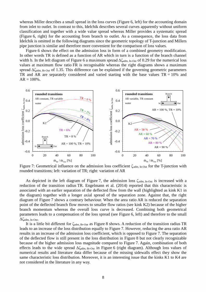
Figure 7: Geometrical influence on the admission loss coefficient adm, In-Out for the T-junction with
rounded transitions; left: variation of TR; right: variation of AR
As depicted in the left diagram of Figure 7, the admission loss adm, In-Out is increased with a
reduction of the transition radius TR. Engelmann et al. (2014) reported that this characteristic is
associated with an earlier separation of the deflected flow from the wall (highlighted as kink K1 in
the diagram) together with a longer axial spread of the separation zone. Against that, the right
diagram of Figure 7 shows a contrary behaviour. When the area ratio AR is reduced the separation
point of the deflected branch flow moves to smaller flow ratios (see kink K2) because of the higher
branch momentum whereas the overall loss curve is decreased. Combining both geometrical
parameters leads to a compensation of the loss spread (see Figure 6, left) and therefore to the small
Δζadm, In-Out.
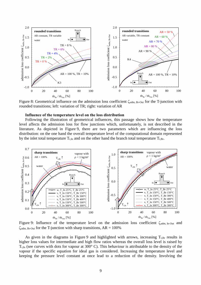
It is a little bit different for ζadm, Br-Out as Figure 8 shows. A reduction of the transition radius TR
leads to an increase of the loss distribution equally to Figure 7. However, reducing the area ratio AR
results in an increase of the admission loss coefficient, which is opposed to Figure 7. The separation
of the deflected flow is still present in the loss distribution in Figure 8 but not clearly recognizable
because of the higher admission loss magnitude compared to Figure 7. Again, combination of both
effects leads to the wide spread Δζadm, Br-Out in Figure 6 (right diagram). Although loss values of
numerical results and literature data differ because of the missing sidewalls effect they show the
same characteristic loss distribution. Moreover, it is an interesting issue that the kinks K1 to K4 are
not considered in the literature in any way.
9
ad
mis
sion
loss
coef
fici
ent
ζ ad
m, B
r-O
ut
-1.0
-0.5
0.0
0.5
1.0
1.5
2.0
0 20 40 60 80 100
T-junction
F0 ru RF 8%
Kurven für A=100% und M in 5% Schritte
R_Fillet = von 1 bis 5mm
[%]m/m OutBr
AR constant, TR variable
TR = 0 %
TR = 8 %
TR = 6%
TR = 4%
TR = 2%
rounded transitions
AR = 100 %, TR = 10%
K3
In Out
Branch
water
adm
issi
on
loss
coef
fici
ent
ζ ad
m, B
r-O
ut
-1.0
-0.5
0.0
0.5
1.0
1.5
2.0
0 20 40 60 80 100
T-junction
Kurven für A=50 bis 100% in 10% und M in 5% Schritte
R_Fillet = konstant 5mm
[%]m/m OutBr
rounded transitions
AR variable, TR constant
AR = 50 %
AR = 100 %, TR = 10%
AR = 60 %
AR = 70 %
AR = 80 %
AR = 90 %
K4
In Out
Branch
water
Figure 8: Geometrical influence on the admission loss coefficient adm, Br-Out for the T-junction with
rounded transitions; left: variation of TR; right: variation of AR
Influence of the temperature level on the loss distribution
Following the illustration of geometrical influences, this passage shows how the temperature
level affects the admission loss for flow junctions which, unfortunately, is not described in the
literature. As depicted in Figure 9, there are two parameters which are influencing the loss
distribution: on the one hand the overall temperature level of the computational domain represented
by the inlet total temperature Tt,In and on the other hand the branch total temperature Tt,Br.
0.0
0.1
0.2
0.3
0.4
0.5
0.6
0.7
0 20 40 60 80 100
w, T_In 25°C, T_Br 25°C
v, T_In 150°C, T_Br 150°C
v, T_In 150°C, T_Br 300°C
v, T_In 150°C, T_Br 400°C
v, T_In 150°C, T_Br 500°C
v, T_In 300°C, T_Br 300°C
adm
issi
on
loss
coef
fici
ent
ζ ad
m, In
-Ou
t
[%]m/m OutBr
sharp transitions
In Out
Branch
water
vapour with
< 1 kg/m³AR = 100% Tt,Br
Tt,In
-1.0
-0.5
0.0
0.5
1.0
0 20 40 60 80 100
w, T_In 25°C, T_Br 25°C
v, T_In 150°C, T_Br 150°C
v, T_In 150°C, T_Br 300°C
v, T_In 150°C, T_Br 400°C
v, T_In 150°C, T_Br 500°C
v, T_In 300°C, T_Br 300°C
adm
issi
on
loss
coef
fici
ent
ζ ad
m, B
r-O
ut
[%]m/m OutBr
sharp transitions
In Out
Branch
AR = 100%
Tt,Br
Tt,In
water
vapour with
< 1 kg/m³
Figure 9: Influence of the temperature level on the admission loss coefficient adm, In-Out and
adm, Br-Out for the T-junction with sharp transitions, AR = 100%
As given in the diagrams in Figure 9 and highlighted with arrows, increasing Tt,Br results in
higher loss values for intermediate and high flow ratios whereas the overall loss level is raised by
Tt,In (see curves with dots for vapour at 300° C). This behaviour is attributable to the density of the
vapour if the specific equation for ideal gas is considered. Increasing the temperature level and
keeping the pressure level constant at once lead to a reduction of the density. Involving the

10
continuity equation for a specific and therefore constant mass flow ratio FR shows that a reduction
of the density leads to a higher channel respectively pipe velocity. This means a higher flow
momentum is present together with higher shear forces within the fluid. But no matter which
temperature is chosen the loss curve for water as incompressible fluid is always located beneath the
corresponding curves for vapour.
Influence of the pressure level on the loss distribution
The pressure level affects the admission loss in the same way as the temperature level does.
Thus, resulting admission loss curves for predictions with several total pressure levels are drawn in
the diagrams of Figure 10. Please note: the total temperature of the numerical domain is raised from
a base value of 150° C up to of 300° C for all corresponding simulations. This is necessary to avoid
a condensation of the overheated steam at 2, 5 and 10 bar. The new base loss curve is plotted with
dots and for comparison already used in Figure 9.
0.0
0.1
0.2
0.3
0.4
0.5
0.6
0.7
0 20 40 60 80 100
w, pt 1bar, Tt 25°C
v, pt 1bar, Tt 150°C
v, pt 1bar, Tt 300°C
v, pt 2 bar, Tt 300°C
v, pt 5 bar, Tt 300°C
v, pt 10 bar, Tt 300°C
adm
issi
on
loss
coef
fici
ent
ζ ad
m, In
-Ou
t
[%]m/m OutBr
sharp transitions
In Out
Branch
vapour with
< 1 kg/m³AR = 100%
pt vapour with
> 1 kg/m³
and water
-1.0
-0.5
0.0
0.5
1.0
0 20 40 60 80 100
w, pt 1bar, Tt 25°C
v, pt 1bar, Tt 150°C
v, pt 1 bar, Tt 300°C
v, pt 2 bar, Tt 300°C
v, pt 5 bar, Tt 300°C
v, pt 10 bar, Tt 300°C
adm
issi
on
loss
coef
fici
ent
ζ ad
m, B
r-O
ut
[%]m/m OutBr
sharp transitions
In Out
Branch
AR = 100%
pt
vapour with
< 1 kg/m³
vapour with
> 1 kg/m³
and water
Figure 10: Influence of the pressure level on the admission loss coefficient adm, In-Out and adm, Br-Out
for the T-junction with sharp transitions, AR = 100%
The arrows in Figure 10 indicate that a higher pressure level leads to a reduction of the
admission loss. This behaviour again is provoked by density shifts in combination with the ideal gas
equation. An increase of the pressure level leads to an increase of the density and therefore reduces
the channel velocity together with corresponding loss inducing effects. As indicated in Figure 9 and
Figure 10, a density of 1 kg/m³ can be seen as limiting value. Values above reduce the admission
loss coefficient while values below increase it.
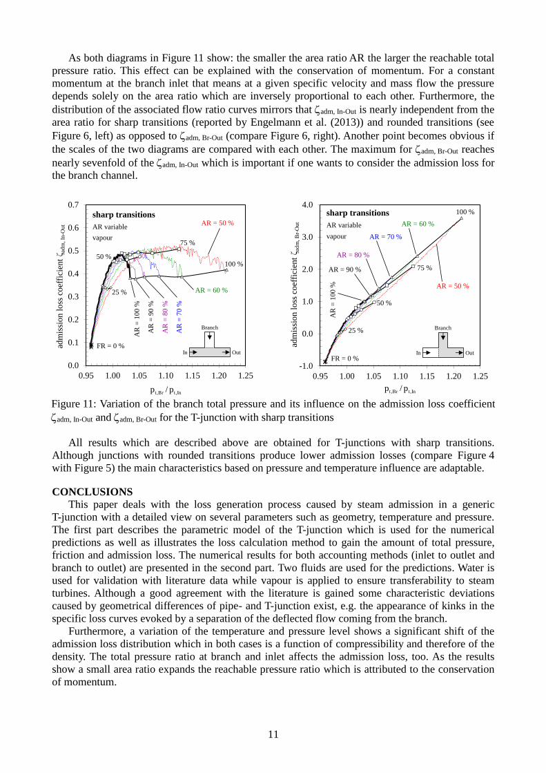
Variation of the pressure ratio and its effect on the admission loss
In prior publications and also in the graphs above all loss curves are generated and drawn as a
function of the flow ratio. But another path is taken in this study. That means in detail not the mass
flow but the total pressure is set as boundary condition at inlet of main and branch channel for the
numerical predictions. The total pressure at the inlet is set to 2 bar whereas the total temperature of
the numerical domain amounts to 300° C. Additionally, the branch total pressure is gradually
increased starting with a total pressure ratio pt,Br / pt,In of 0.95 up to a maximum of 1.25. The
corresponding mass flow ratios are calculated during the simulations as function of the actual total
pressure ratio. The resulting admission loss curves for several area ratios are given in Figure 11
whereas specific flow ratios FR using a step size of 25% are highlighted with symbols.
11
As both diagrams in Figure 11 show: the smaller the area ratio AR the larger the reachable total
pressure ratio. This effect can be explained with the conservation of momentum. For a constant
momentum at the branch inlet that means at a given specific velocity and mass flow the pressure
depends solely on the area ratio which are inversely proportional to each other. Furthermore, the
distribution of the associated flow ratio curves mirrors that adm, In-Out is nearly independent from the
area ratio for sharp transitions (reported by Engelmann et al. (2013)) and rounded transitions (see
Figure 6, left) as opposed to adm, Br-Out (compare Figure 6, right). Another point becomes obvious if
the scales of the two diagrams are compared with each other. The maximum for adm, Br-Out reaches
nearly sevenfold of theadm, In-Out which is important if one wants to consider the admission loss for
the branch channel.
0.0
0.1
0.2
0.3
0.4
0.5
0.6
0.7
0.95 1.00 1.05 1.10 1.15 1.20 1.25
AR = 100%
AR = 90%
AR = 80%
AR = 70%
AR = 60% ändern
AR = 50% ändern
FR 0%
Fr 25%
FR 50%
FR 75%
FR 100%
Variation des PT von Bleed von 1.9 bis 2.1
In,tBr,t p/p
adm
issi
on
loss
coef
fici
ent
ζ ad
m, In
-Ou
t
sharp transitions
In Out
Branch
AR variable
vapour
AR = 50 %
AR
= 1
00
%
AR = 60 %
AR
= 7
0 %
AR
= 8
0 %
AR
= 9
0 %
100 %
75 %
50 %
25 %
FR = 0 %
-1.0
0.0
1.0
2.0
3.0
4.0
0.95 1.00 1.05 1.10 1.15 1.20 1.25
AR = 100%
AR = 90%
AR = 80%
AR = 70%
AR = 60% ändern
AR = 50% ändern
FR 0%
Fr 25%
FR 50%
FR 75%
FR 100%
Variation des PT von Bleed von 1.9 bis 2.1
In,tBr,t p/p
adm
issi
on
loss
coef
fici
ent
ζ ad
m, B
r-O
ut
sharp transitions
In Out
Branch
AR variable
vapour
FR = 0 %
25 %
50 %
100 %
75 %
AR = 50 %
AR
= 1
00
%
AR = 60 %
AR = 70 %
AR = 80 %
AR = 90 %
Figure 11: Variation of the branch total pressure and its influence on the admission loss coefficient
adm, In-Out and adm, Br-Out for the T-junction with sharp transitions
All results which are described above are obtained for T-junctions with sharp transitions.
Although junctions with rounded transitions produce lower admission losses (compare Figure 4
with Figure 5) the main characteristics based on pressure and temperature influence are adaptable.
CONCLUSIONS
This paper deals with the loss generation process caused by steam admission in a generic
T-junction with a detailed view on several parameters such as geometry, temperature and pressure.
The first part describes the parametric model of the T-junction which is used for the numerical
predictions as well as illustrates the loss calculation method to gain the amount of total pressure,
friction and admission loss. The numerical results for both accounting methods (inlet to outlet and
branch to outlet) are presented in the second part. Two fluids are used for the predictions. Water is
used for validation with literature data while vapour is applied to ensure transferability to steam
turbines. Although a good agreement with the literature is gained some characteristic deviations
caused by geometrical differences of pipe- and T-junction exist, e.g. the appearance of kinks in the
specific loss curves evoked by a separation of the deflected flow coming from the branch.
Furthermore, a variation of the temperature and pressure level shows a significant shift of the
admission loss distribution which in both cases is a function of compressibility and therefore of the
density. The total pressure ratio at branch and inlet affects the admission loss, too. As the results
show a small area ratio expands the reachable pressure ratio which is attributed to the conservation
of momentum.

12
Unfortunately, in literature admission loss information for compressible fluids are not provided
to date. Thus, it is recommended to build up a test rig including the described generic junction in
order to gather appropriate validation data and to prove the characteristic flow effects. Further
numerical work will deal with the influences of inflow angle variations, a mixed accounting
considering inlet, branch and outlet at the same time as well as with more predictions of steam
turbine sections.
REFERENCES
Andersson, U., Westin, J., Eriksson, J., 2006. Thermal Mixing in a T-junction. Tech. Rep. U 06-66,
Vattenfall Research and Development AB.
Barringer, M., Thole, K. A., Krishan, V. and Landrum, E. (2014), “Manufacturing Influences On
Pressure Losses of Channel Fed Holes”, Trans. ASME, Journal of Turbomachinery”, Vol. 136,
pp 051012-1-10.
Denton, J. (1993), “Loss Mechanisms in Turbomachines”, Trans. ASME, Journal of
Turbomachinery, Vol. 115, pp 21-656.
Engelmann, D., Schramm, A., Polklas, T. and Mailach, R., (2014), “Losses of Steam Admission in
Industrial Steam Turbines Depending on Geometrical Parameters”, ASME Turbo Expo, Paper-No.
GT2014- 25172.
Engelmann, D., Schramm, A., Polklas, T., Schwarz, M., A. & Mailach, R. (2013), “Enhanced Loss
Prediction for Admission through Circumferential Slots in Axial Steam Turbines”, Conference
Proceedings of the 10th European Conference on Turbomachinery, pp 350-359.
Engelmann, D., Kalkkuhl, T. J., Polklas, T. and Mailach, R. (2012), “Influence of Shroud Cavity Jet
and Steam Admission through a Circumferential Slot on the Flow Field in a Steam Turbine”, ASME
Turbo Expo, Paper-No. GT2012-68465.
Gier, J., Stubert, B., Brouillet, B. and de Vito, L. (2003), “Interaction of Shroud Leakage Flow and
Main Flow in a Three-Stage LP Turbine”, ASME Turbo Expo, Paper-No. GT2003-38025.
Idelchik, I. E. (1986): “Handbook of Hydraulic Resistance (2nd Edition)”, Hemisphere Publishes,
Diagrams 7-4 & 7-11.
Kuczaj, A. K., Komen, E.M.J. and Loginov, M.S. (2010) “Large-Eddy Simulation study of turbulent
mixing in a T-junction”, Nuclear Engineering and Design, Vol. 240, pp 2116–2122.
Miller, D. S. (1990): “Internal Flow Systems (2nd Edition)”, British Hydromechanics Research
Association, Figures 13.10, 13.11, 13.14 & 13.15.
Schlichting, H. and Gersten, K. (2006), „Grenzschicht-Theorie“, 10th Edition, Springer, Berlin.
Walker, C., Manera, A., Niceno, B., Simiano, M. and Prasser, H.-M. (2010), “Steady-state RANS-
simulations of the mixing in a T-junction”, Nuclear Engineering and Design, Vol. 240,
pp 2107-2115.
Wallis, A. M., Denton, J. D. and Demarge, A. A. J. (2000), “The Control of Shroud Leakage Flows
to Reduce Aerodynamic Losses in a Low Aspect Ratio Shrouded Axial Flow Turbine”, ASME
Turbo Expo, Paper-No. 2000-GT-475.