Embed Size (px)
Citation preview
A Design Flow for the Development, Characterization,and Refinement of System Level Architectural
Services
Douglas Michael Densmore
Electrical Engineering and Computer SciencesUniversity of California at Berkeley
Technical Report No. UCB/EECS-2007-59
http://www.eecs.berkeley.edu/Pubs/TechRpts/2007/EECS-2007-59.html
May 16, 2007

Copyright © 2007, by the author(s).All rights reserved.
Permission to make digital or hard copies of all or part of this work forpersonal or classroom use is granted without fee provided that copies arenot made or distributed for profit or commercial advantage and that copiesbear this notice and the full citation on the first page. To copy otherwise, torepublish, to post on servers or to redistribute to lists, requires prior specificpermission.
A Design Flow for the Development, Characterization, and Refinement of System LevelArchitectural Services
by
Douglas Michael Densmore
B.S. (University of Michigan, Ann Arbor) 2001M.S. (University of California, Berkeley) 2004
A dissertation submitted in partial satisfaction of therequirements for the degree of
Doctor of Philosophy
in
Engineering - Electrical Engineering and Computer Sciences
in the
GRADUATE DIVISIONof the
UNIVERSITY OF CALIFORNIA, BERKELEY
Committee in charge:Professor Alberto Sangiovanni-Vincentelli, Chair
Professor Jan RabaeyProfessor Lee Schruben
Spring 2007

The dissertation of Douglas Michael Densmore is approved:
Chair Date
Date
Date
University of California, Berkeley
Spring 2007

A Design Flow for the Development, Characterization, and Refinement of System Level
Architectural Services
Copyright 2007
by
Douglas Michael Densmore
1
Abstract
A Design Flow for the Development, Characterization, and Refinement of System Level
Architectural Services
by
Douglas Michael Densmore
Doctor of Philosophy in Engineering - Electrical Engineering and Computer Sciences
University of California, Berkeley
Professor Alberto Sangiovanni-Vincentelli, Chair
The electronics industry is facing serious challenges because of the increased demand on func-
tionality and strong pressures on both time-to-market and cost requirements. The complexity designers have
to deal with creates design quality problems that force serious delays in product introductions and even prod-
uct recalls. There is a need for methodologies and tools that can drastically reduce design errors and costs.
Electronic System Level (ESL) tools attempt to fulfill this need by increasing the abstraction and modularity
by which designs can be specified. However, simply because these design styles are introduced, this does
not automatically imply an acceptable level of accuracy and efficiency required for widespread adoption
and eventual success. This thesis introduces a design flow which improves abstraction and modularity while
remaining highly accurate and efficient. Specifically this work explores a Platform-Based Design approach
to model architectural services.
Platform-Based Design is a methodology in which purely functional descriptions of a system are
top-down assigned (or mapped) to architecture services which have their models for capabilities and costs
exported from the bottom up. Architecture services are a set of library elements characterized by their
capabilities (what functionality they support) and costs (execution time, power, etc). These libraries of
components “parametrize” the set of architecture services that can be chosen by the designer to implement
functionality and limit the design space thus favoring design re-use. The design process then proceeds
toward implementation by binding functionality to architectures composed of elements from the library.
The components that form a platform instance are selected by evaluating their capability of supporting the
mapped functionality within the design constraints and by optimizing objective functions. The design space
exploration can be done via simulation of the mapped designs by changing the mapping and the choice of
2
components. Keeping the architecture services and the functional aspects of the design separate facilitates
design space exploration since this exploration requires only the change of the mapping of functions to
architectural services or the selection of a different set of components to build the platform instance. In
either case, only a minor change to the description of the design is required to perform the evaluation.
The design flow proposed in this thesis specifically focuses on how to create architecture service
models of programmable platforms (FPGAs for example). These architecture service models are created
at the transaction level, are preemptable, and export their abilities to the mapping process. An architecture
service library is described for Xilinx’s Virtex II Pro FPGA. If this library is used, a method exists to extract
the architecture topology to program an FPGA device directly, thus avoiding error prone manual techniques.
As a consequence of this programmable platform modeling style, the models can be annotated directly with
characterization data from a concurrent characterization process to be described.
Finally, in order to support various levels of abstraction in these architecture service models, a
refinement verification flow will be discussed as well. Three styles will be proposed each with their own
emphasis (event based, interface based, compositional component based). They are each deployed depend-
ing on the designer’s needs and the environment in which the architecture is developed. These needs include
changing the topology of the architecture model, modifying the operation of the architecture service, and the
exploring the tradeoffs between how one expresses the services themselves and the simulation infrastructure
which schedules the use of those services.
To provide a proof of concept of these techniques, several design scenarios are explored. These
scenarios include Motion-JPEG encoding, an H.264 deblocking filter, an SPI-5 networking protocol, and
a communication structure of a highly concurrent system architecture (FLEET). The results show that not
only is the proposed design flow more accurate and modular than other approaches but also that it prevents
the selection of more poorly performing designs or the selection of incorrectly functioning designs through
its emphasis on the preservation of fidelity.
Professor Alberto Sangiovanni-VincentelliDissertation Committee Chair

i
For Mom and Dad
When you comin’ home son? I don’t know when, but we’ll get together then...
Para Remolachita
¡Colorın colorado, esta tesis se ha acabado! Besitos
ii
Contents
List of Figures v
List of Tables viii
1 Introduction 11.0.1 Chapter Organization . . . . . . . . . . . . . . . . . . . . . . . . . . . . . . . . . . 5
1.1 Motivating Factors . . . . . . . . . . . . . . . . . . . . . . . . . . . . . . . . . . . . . . . 61.1.1 Heterogeneity . . . . . . . . . . . . . . . . . . . . . . . . . . . . . . . . . . . . . . 61.1.2 Complexity . . . . . . . . . . . . . . . . . . . . . . . . . . . . . . . . . . . . . . . 91.1.3 Time to Market . . . . . . . . . . . . . . . . . . . . . . . . . . . . . . . . . . . . . 11
1.2 1st Focus: System Level Design . . . . . . . . . . . . . . . . . . . . . . . . . . . . . . . . 121.3 2nd Focus: Programmable Architecture Services . . . . . . . . . . . . . . . . . . . . . . . 151.4 Thesis Contribution . . . . . . . . . . . . . . . . . . . . . . . . . . . . . . . . . . . . . . . 20
1.4.1 Naıve Design Flow . . . . . . . . . . . . . . . . . . . . . . . . . . . . . . . . . . . 211.4.2 Proposed Design Flow . . . . . . . . . . . . . . . . . . . . . . . . . . . . . . . . . 21
1.5 Thesis Outline . . . . . . . . . . . . . . . . . . . . . . . . . . . . . . . . . . . . . . . . . . 23
2 System Level Architecture Services 252.0.1 Chapter Organization . . . . . . . . . . . . . . . . . . . . . . . . . . . . . . . . . . 27
2.1 Background and Basic Definitions . . . . . . . . . . . . . . . . . . . . . . . . . . . . . . . 282.2 Related Work . . . . . . . . . . . . . . . . . . . . . . . . . . . . . . . . . . . . . . . . . . 312.3 System Level Event Based Architecture Services . . . . . . . . . . . . . . . . . . . . . . . 34
2.3.1 METROPOLIS Architecture Construction . . . . . . . . . . . . . . . . . . . . . . . 362.3.2 METRO II Architecture Construction . . . . . . . . . . . . . . . . . . . . . . . . . 412.3.3 Architecture Service Extensions . . . . . . . . . . . . . . . . . . . . . . . . . . . . 44
2.4 Xilinx Architecture Modeling Exploration . . . . . . . . . . . . . . . . . . . . . . . . . . . 482.5 FLEET Architecture Modeling Exploration . . . . . . . . . . . . . . . . . . . . . . . . . . 622.6 Synthesis Path for Architecture Services . . . . . . . . . . . . . . . . . . . . . . . . . . . . 642.7 Conclusions . . . . . . . . . . . . . . . . . . . . . . . . . . . . . . . . . . . . . . . . . . . 66
3 Architecture Service Characterization 673.0.1 Chapter Organization . . . . . . . . . . . . . . . . . . . . . . . . . . . . . . . . . . 70
3.1 Platform Characterization . . . . . . . . . . . . . . . . . . . . . . . . . . . . . . . . . . . . 703.1.1 Characterization Requirements . . . . . . . . . . . . . . . . . . . . . . . . . . . . . 71
iii
3.2 Extraction of Platform Characterization Data . . . . . . . . . . . . . . . . . . . . . . . . . 723.2.1 Data Extraction Requirements . . . . . . . . . . . . . . . . . . . . . . . . . . . . . 73
3.3 Example Platform Characterization . . . . . . . . . . . . . . . . . . . . . . . . . . . . . . . 753.4 Organization of Platform Characterization Data . . . . . . . . . . . . . . . . . . . . . . . . 78
3.4.1 Data Categorization . . . . . . . . . . . . . . . . . . . . . . . . . . . . . . . . . . 783.4.2 Data Storage Structure . . . . . . . . . . . . . . . . . . . . . . . . . . . . . . . . . 79
3.5 Integration of Platform Characterization and Architectural Services . . . . . . . . . . . . . . 803.5.1 Sample Annotation Semantics . . . . . . . . . . . . . . . . . . . . . . . . . . . . . 82
3.6 Conclusions . . . . . . . . . . . . . . . . . . . . . . . . . . . . . . . . . . . . . . . . . . . 83
4 System Level Service Refinement 854.0.1 Chapter Organization . . . . . . . . . . . . . . . . . . . . . . . . . . . . . . . . . . 87
4.1 Background and Basic Definitions . . . . . . . . . . . . . . . . . . . . . . . . . . . . . . . 874.1.1 State Equivalence . . . . . . . . . . . . . . . . . . . . . . . . . . . . . . . . . . . . 884.1.2 Trace Containment . . . . . . . . . . . . . . . . . . . . . . . . . . . . . . . . . . . 894.1.3 Synchronized Parallel Composition . . . . . . . . . . . . . . . . . . . . . . . . . . 89
4.2 Related Work . . . . . . . . . . . . . . . . . . . . . . . . . . . . . . . . . . . . . . . . . . 914.3 Event Based Service Refinement . . . . . . . . . . . . . . . . . . . . . . . . . . . . . . . . 97
4.3.1 Proposed Methodology . . . . . . . . . . . . . . . . . . . . . . . . . . . . . . . . . 984.4 Interface Based Service Refinement . . . . . . . . . . . . . . . . . . . . . . . . . . . . . . 113
4.4.1 Proposed Methodology . . . . . . . . . . . . . . . . . . . . . . . . . . . . . . . . . 1144.5 Compositional Component Based Service Refinement . . . . . . . . . . . . . . . . . . . . . 132
4.5.1 Proposed Methodology . . . . . . . . . . . . . . . . . . . . . . . . . . . . . . . . . 1324.6 Conclusions . . . . . . . . . . . . . . . . . . . . . . . . . . . . . . . . . . . . . . . . . . . 138
5 Design Flow Examples 1405.0.1 Chapter Organization . . . . . . . . . . . . . . . . . . . . . . . . . . . . . . . . . . 142
5.1 Characterization Aided Fidelity Example: Motion-JPEG . . . . . . . . . . . . . . . . . . . 1425.2 Service Aided Mapping Modularity Example: H.264 Deblocking Filter . . . . . . . . . . . 144
5.2.1 Application Details . . . . . . . . . . . . . . . . . . . . . . . . . . . . . . . . . . . 1465.2.2 Mapping Details . . . . . . . . . . . . . . . . . . . . . . . . . . . . . . . . . . . . 1475.2.3 Design Space Exploration Results . . . . . . . . . . . . . . . . . . . . . . . . . . . 150
5.3 Architecture Platform Refinement Example: SPI5 Packet Processing . . . . . . . . . . . . . 1545.3.1 Application Parameters . . . . . . . . . . . . . . . . . . . . . . . . . . . . . . . . . 1555.3.2 Architecture Parameters . . . . . . . . . . . . . . . . . . . . . . . . . . . . . . . . 1555.3.3 Refinement Based Design Flow . . . . . . . . . . . . . . . . . . . . . . . . . . . . 1575.3.4 Platform Development . . . . . . . . . . . . . . . . . . . . . . . . . . . . . . . . . 1575.3.5 METROPOLIS Models . . . . . . . . . . . . . . . . . . . . . . . . . . . . . . . . . 1625.3.6 Results . . . . . . . . . . . . . . . . . . . . . . . . . . . . . . . . . . . . . . . . . 163
5.4 Communication Subsystem Refinement Example: FLEET Communication Structure . . . . 1665.4.1 Communication Library . . . . . . . . . . . . . . . . . . . . . . . . . . . . . . . . 1665.4.2 Verification Process . . . . . . . . . . . . . . . . . . . . . . . . . . . . . . . . . . . 170

iv
6 Conclusions and Contributions 1746.0.3 Chapter Organization . . . . . . . . . . . . . . . . . . . . . . . . . . . . . . . . . . 175
6.1 Benefits . . . . . . . . . . . . . . . . . . . . . . . . . . . . . . . . . . . . . . . . . . . . . 1756.2 Disadvantages . . . . . . . . . . . . . . . . . . . . . . . . . . . . . . . . . . . . . . . . . . 1766.3 Future Work . . . . . . . . . . . . . . . . . . . . . . . . . . . . . . . . . . . . . . . . . . . 177
6.3.1 Integration . . . . . . . . . . . . . . . . . . . . . . . . . . . . . . . . . . . . . . . 1786.3.2 Formalism . . . . . . . . . . . . . . . . . . . . . . . . . . . . . . . . . . . . . . . 1786.3.3 Extensions . . . . . . . . . . . . . . . . . . . . . . . . . . . . . . . . . . . . . . . 179
Bibliography 180
v
List of Figures
1.1 Overall EDA Revenue Growth and EDA Design Segment Growth [Ric05] . . . . . . . . . . 21.2 “Methodology Gap” Challenge in EDA . . . . . . . . . . . . . . . . . . . . . . . . . . . . 31.3 Global Embedded Systems Market [Rav05] . . . . . . . . . . . . . . . . . . . . . . . . . . 71.4 Semiconductor Design Cycle Time Decline [Gar05a] . . . . . . . . . . . . . . . . . . . . . 71.5 Technological SoC Heterogeneity [Don04] . . . . . . . . . . . . . . . . . . . . . . . . . . . 71.6 Device Component and Communication Heterogeneity [Int06b] . . . . . . . . . . . . . . . 81.7 Growing Gap Between Device Capacity and Designer Productivity [Int99] . . . . . . . . . . 101.8 Time to Market Revenue Consequences [IBM06] . . . . . . . . . . . . . . . . . . . . . . . 111.9 Platform-Based Design Methodology [Alb02] . . . . . . . . . . . . . . . . . . . . . . . . . 141.10 METROPOLIS Design Environment and Organization . . . . . . . . . . . . . . . . . . . . . 151.11 Makimoto’s Wave and Programmable Devices [Tsu00] . . . . . . . . . . . . . . . . . . . . 171.12 Naıve Design Flow . . . . . . . . . . . . . . . . . . . . . . . . . . . . . . . . . . . . . . . 221.13 Proposed Design Flow . . . . . . . . . . . . . . . . . . . . . . . . . . . . . . . . . . . . . 24
2.1 Proposed Service Style Versus Existing Service Styles . . . . . . . . . . . . . . . . . . . . 272.2 System Level Architecture Modeling in the Proposed Flow . . . . . . . . . . . . . . . . . . 282.3 Architecture Platform Composition and Creation . . . . . . . . . . . . . . . . . . . . . . . 292.4 Architecture Service Taxonomy . . . . . . . . . . . . . . . . . . . . . . . . . . . . . . . . 292.5 Composing Architectures Using Services . . . . . . . . . . . . . . . . . . . . . . . . . . . 372.6 METROPOLIS Process Example Code . . . . . . . . . . . . . . . . . . . . . . . . . . . . . 382.7 METROPOLIS Medium Example Code . . . . . . . . . . . . . . . . . . . . . . . . . . . . . 382.8 METROPOLIS Quantity Manager Example Code . . . . . . . . . . . . . . . . . . . . . . . . 392.9 METROPOLIS State Media Example Code . . . . . . . . . . . . . . . . . . . . . . . . . . . 392.10 METROPOLIS Port Interface Example Code . . . . . . . . . . . . . . . . . . . . . . . . . . 402.11 METROPOLIS Architecture Netlists . . . . . . . . . . . . . . . . . . . . . . . . . . . . . . 412.12 Graphical METROPOLIS Architecture Representation . . . . . . . . . . . . . . . . . . . . . 422.13 Architecture Service Model Proposal in METRO II . . . . . . . . . . . . . . . . . . . . . . 442.14 Architecture Extensions for Preemption . . . . . . . . . . . . . . . . . . . . . . . . . . . . 452.15 Architecture Extensions for Mapping . . . . . . . . . . . . . . . . . . . . . . . . . . . . . . 482.16 METROPOLIS PowerPC Model . . . . . . . . . . . . . . . . . . . . . . . . . . . . . . . . . 532.17 METROPOLIS MicroBlaze Model . . . . . . . . . . . . . . . . . . . . . . . . . . . . . . . 552.18 METROPOLIS Synthetic Master/Slave Model . . . . . . . . . . . . . . . . . . . . . . . . . 562.19 METROPOLIS PLB Model . . . . . . . . . . . . . . . . . . . . . . . . . . . . . . . . . . . 57
vi
2.20 METROPOLIS OPB Model . . . . . . . . . . . . . . . . . . . . . . . . . . . . . . . . . . . 582.21 METROPOLIS BRAM Model . . . . . . . . . . . . . . . . . . . . . . . . . . . . . . . . . . 602.22 METROPOLIS Quantity Manager Model . . . . . . . . . . . . . . . . . . . . . . . . . . . . 622.23 FLEET SHIP Architecture . . . . . . . . . . . . . . . . . . . . . . . . . . . . . . . . . . . 632.24 FLEET Services Created . . . . . . . . . . . . . . . . . . . . . . . . . . . . . . . . . . . . 652.25 Automatic Xilinx MHS Extraction . . . . . . . . . . . . . . . . . . . . . . . . . . . . . . . 66
3.1 Transcending RTL Effort with ESL Design Technologies . . . . . . . . . . . . . . . . . . . 683.2 Characterization of Architecture Services in the Proposed Design Flow . . . . . . . . . . . . 693.3 A Design Flow for Pre-characterizing Programmable Platforms . . . . . . . . . . . . . . . . 743.4 Combo Systems Resource Usage and Performance . . . . . . . . . . . . . . . . . . . . . . 763.5 PowerPC System Performance Analysis . . . . . . . . . . . . . . . . . . . . . . . . . . . . 773.6 Characterized Data Organization Proposal . . . . . . . . . . . . . . . . . . . . . . . . . . . 813.7 METROPOLIS Sample Annotation Semantics Using Characterized Data . . . . . . . . . . . 83
4.1 System Level Service Refinement in the Proposed Design Flow . . . . . . . . . . . . . . . . 864.2 METROPOLIS Style Refinement Example . . . . . . . . . . . . . . . . . . . . . . . . . . . 944.3 Event Based Refinement Proposal . . . . . . . . . . . . . . . . . . . . . . . . . . . . . . . 994.4 Vertical Refinement Illustration in METROPOLIS . . . . . . . . . . . . . . . . . . . . . . . 1014.5 Horizontal Refinement Illustration in METROPOLIS . . . . . . . . . . . . . . . . . . . . . . 1044.6 Macro and MicroProperty Relationships . . . . . . . . . . . . . . . . . . . . . . . . . . . . 1114.7 Event Petri Net Example . . . . . . . . . . . . . . . . . . . . . . . . . . . . . . . . . . . . 1144.8 Interface Based Refinement Proposal . . . . . . . . . . . . . . . . . . . . . . . . . . . . . . 1154.9 Refinement Domains in Interface Based Refinement . . . . . . . . . . . . . . . . . . . . . . 1184.10 METROPOLIS Code Example . . . . . . . . . . . . . . . . . . . . . . . . . . . . . . . . . . 1204.11 Resulting CFA for Code Example . . . . . . . . . . . . . . . . . . . . . . . . . . . . . . . 1204.12 CFA Visual Representation . . . . . . . . . . . . . . . . . . . . . . . . . . . . . . . . . . . 1224.13 CFA FSM Representation . . . . . . . . . . . . . . . . . . . . . . . . . . . . . . . . . . . . 1234.14 SIS Commands and EXLIF Requirements for FORTE Flow . . . . . . . . . . . . . . . . . . 1284.15 Surface Refinement Flows for METROPOLIS . . . . . . . . . . . . . . . . . . . . . . . . . . 1314.16 Strict Transition Refinement . . . . . . . . . . . . . . . . . . . . . . . . . . . . . . . . . . 1364.17 Stuttering Transition Refinement . . . . . . . . . . . . . . . . . . . . . . . . . . . . . . . . 1364.18 Lack of τ-Divergence . . . . . . . . . . . . . . . . . . . . . . . . . . . . . . . . . . . . . . 1364.19 External Non-Determinism Preservation . . . . . . . . . . . . . . . . . . . . . . . . . . . . 1364.20 .fts for Abstract Consumer LTS . . . . . . . . . . . . . . . . . . . . . . . . . . . . . . . . . 1374.21 .fts for Refined Consumer LTS . . . . . . . . . . . . . . . . . . . . . . . . . . . . . . . . . 1374.22 .inv for Consumer LTSs . . . . . . . . . . . . . . . . . . . . . . . . . . . . . . . . . . . . . 1384.23 .sync for Producer/Consumer LTSs . . . . . . . . . . . . . . . . . . . . . . . . . . . . . . . 139
5.1 MJPEG Architecture Topologies in METROPOLIS . . . . . . . . . . . . . . . . . . . . . . . 1435.2 Macroblock and Block Border Illustration for H.264 Deblocking Filter . . . . . . . . . . . . 1465.3 Deblocking Filter Pseudo Code . . . . . . . . . . . . . . . . . . . . . . . . . . . . . . . . . 1475.4 Decomposition of GetStrength Function . . . . . . . . . . . . . . . . . . . . . . . . . . . . 1485.5 Decomposition of EdgeLoop Function . . . . . . . . . . . . . . . . . . . . . . . . . . . . . 1485.6 Mapping a Functional Model onto an Architectural Model for H.264 . . . . . . . . . . . . . 149

vii
5.7 H.264 Functional Topology Mapping Candidates . . . . . . . . . . . . . . . . . . . . . . . 1505.8 METROPOLIS H.264 Simulation Results for All Candidate Topologies . . . . . . . . . . . . 1515.9 METROPOLIS H.264 Simulation Results for Various FIFO Sizes . . . . . . . . . . . . . . . 1525.10 METROPOLIS H.264 Accuracy Versus FPGA Implementation . . . . . . . . . . . . . . . . 1545.11 Successive Platform Refinement Methodology . . . . . . . . . . . . . . . . . . . . . . . . . 1585.12 Platform Development for SPI-5 . . . . . . . . . . . . . . . . . . . . . . . . . . . . . . . . 1595.13 METROPOLIS Architecture Model for Platform 2.2 . . . . . . . . . . . . . . . . . . . . . . 1635.14 Sample Control Flow Automata for Abstract and Refined FIFO Scheduler . . . . . . . . . . 1645.15 FIFO Occupancy Data for Platform 2.1 and 2.2 . . . . . . . . . . . . . . . . . . . . . . . . 1655.16 LTS Communication Example #1 for FLEET . . . . . . . . . . . . . . . . . . . . . . . . . 1675.17 LTS Communication Example #2 for FLEET . . . . . . . . . . . . . . . . . . . . . . . . . 1685.18 LTS Communication Example #3 for FLEET . . . . . . . . . . . . . . . . . . . . . . . . . 1695.19 FLEET System Architecture Service Refinement Opportunities . . . . . . . . . . . . . . . . 1705.20 LTS for Entire FLEET System Level Service Models . . . . . . . . . . . . . . . . . . . . . 172
viii
List of Tables
1.1 Relationship Between Factors, Solutions, Supporting Techniques, and Outcomes . . . . . . 51.2 Characteristics of Programmable Platforms . . . . . . . . . . . . . . . . . . . . . . . . . . 181.3 Programmable Platform Technology Classification . . . . . . . . . . . . . . . . . . . . . . 181.4 Example Programmable Platform Architecture Classifications . . . . . . . . . . . . . . . . 191.5 Horizontal/Vertical Axis Classification Example [Pat01] . . . . . . . . . . . . . . . . . . . 191.6 Contributions of this Thesis . . . . . . . . . . . . . . . . . . . . . . . . . . . . . . . . . . . 23
2.1 Comparison of Architecture Service Modeling Approaches . . . . . . . . . . . . . . . . . . 342.2 PowerPC store instructions . . . . . . . . . . . . . . . . . . . . . . . . . . . . . . . . . . . 542.3 PowerPC load instructions . . . . . . . . . . . . . . . . . . . . . . . . . . . . . . . . . . . 542.4 PowerPC Service Performance Estimation Summary . . . . . . . . . . . . . . . . . . . . . 542.5 MicroBlaze Service Performance Estimation Summary . . . . . . . . . . . . . . . . . . . . 552.6 PLB Bus Service Performance Estimation Summary . . . . . . . . . . . . . . . . . . . . . 582.7 OPB Bus Service Performance Estimation Summary . . . . . . . . . . . . . . . . . . . . . 592.8 Memory Service Performance Estimation Summary . . . . . . . . . . . . . . . . . . . . . . 61
3.1 Performance Characterization Tradeoffs . . . . . . . . . . . . . . . . . . . . . . . . . . . . 713.2 Example CoreConnect Based System Permutations for Characterization . . . . . . . . . . . 753.3 Non-linear Performance Observed in PPC Systems . . . . . . . . . . . . . . . . . . . . . . 773.4 Sample Simulation Using Characterization Data . . . . . . . . . . . . . . . . . . . . . . . . 79
4.1 Refinement Verification Related Work Classification . . . . . . . . . . . . . . . . . . . . . 924.2 Potential Vertical Refinement Event Traces . . . . . . . . . . . . . . . . . . . . . . . . . . 1014.3 Potential Horizontal Refinement Event Traces . . . . . . . . . . . . . . . . . . . . . . . . . 1044.4 Resource Utilization Event Analysis . . . . . . . . . . . . . . . . . . . . . . . . . . . . . . 1064.5 Latency Event Analysis . . . . . . . . . . . . . . . . . . . . . . . . . . . . . . . . . . . . . 1074.6 Asymptotic Analysis of Surface Refinement Flows . . . . . . . . . . . . . . . . . . . . . . 132
5.1 MJPEG Encoding Simulation Performance Analysis . . . . . . . . . . . . . . . . . . . . . 1445.2 H.264 Performance and Cost Results for All Topologies . . . . . . . . . . . . . . . . . . . . 1535.3 Example of SPI-5 Data Generation Using the Architecture and Application Parameters . . . 1565.4 SPI-5 Application Parameter Interaction . . . . . . . . . . . . . . . . . . . . . . . . . . . . 1605.5 Traces from FIFO Scheduler CFAs . . . . . . . . . . . . . . . . . . . . . . . . . . . . . . . 1655.6 FLEET LTS States and Transitions . . . . . . . . . . . . . . . . . . . . . . . . . . . . . . . 173

ix
Acknowledgments
I would first like to thank my advisor Alberto Sangiovanni-Vincentelli. Not only for his support in helping
me to complete this thesis (and by implication my graduate student career), but also for his mentorship,
advice, and leadership. As I go forward in my career I will forever benefit from our interaction and I hope
that I can be an example to other students some day as he was to me.
Naturally I need to acknowledge all the wonderful fellow graduate students I have worked with
over the past 6+ years while at Berkeley. In particular Abhijit Davare, Qi Zhu, Trevor Meyerowitz, Alessan-
dro Pinto, Guang Yang, Mark McKelvin, Donald Chai, Matt Moskewicz, and Will Plishker. I enjoyed our
many interactions both academic and otherwise. I look forward to when our paths cross again. Best of luck
in all your future endeavors.
Additionally, although not listed explicitly here, all the residents of the Donald O. Peterson (DOP)
Center (Alberto’s group in particular), many other EECS graduate students, and Berkeley students in general
were a pleasure to spend time with. I wish them all the best not only in their studies but in all aspects of
their life. Hopefully we will one day realize what an honor it was to study at a place like Berkeley. It is
impossible to list everyone important to me here. In the event of an omission, know that you are still in my
heart.
As a UC Berkeley graduate student I have had the pleasure of working with some of the best
researchers in the world. My discussions with Ivan Sutherland, Yoshi Watanabe, Shinjiro Kakita, Samar
Abdi, Felice Balarin, Luciano Lavagno, Marly Roncken, John Moondanos, Jason Cong, Adam Donlin,
Patrick Lysaght, John Wawrzynek, Dan Garcia, Edward Lee, and David Patterson were truly inspirational
and I am a better person as a result of our interaction. Thanks for the doors you opened and continue to open
for me both in terms of my career and intellectually.
As every researcher knows, nothing gets done without a tremendous support staff. The Berkeley
staff and administrators such as Sheila Humphreys, Colette Patt, Ruth Gjerde, Mary Byrnes, Beatriz Lopez-
Flores, Loretta Lutcher, and Carla Trujillo gave Berkeley a human touch and on some level they are the
reason that I came to Berkeley. They are extremely dedicated folks and a true asset to the university. Thanks
for everything!
While at Berkeley I was involved in various student groups such as BGESS, LAGSES and HKN.
Fellow members of these groups such as Noaa Avital, Kofi Boakye, Nerayo Neclemariam, Lisa Angus,
Fabian Beltran, Esther Zeledon, Rey Guerra, Hakim Weatherspoon (Makda and the kids too), Rob Crockett,
and Greg Lawrence provided the extra laugh or pat on the back that made all the difference.
A number of companies have supported me throughout the years as well. Intel in particular has

x
been amazing providing me with 4 internships and two fellowships. They gave me a chance when I was
a 20 year old sophomore with little experience. Without this co-op experience I would not have had the
confidence to know that I could be a successful engineer. Xilinx and Cypress semiconductor as well have
been open to my research and supported me during internships and provided me with equipment during my
time as a grad student. Cadence Berkeley Lab was also vital in my early development as a researcher.
Naturally I am indebted to other my other readers as well. Prof. Jan Rabaey’s and Prof. Lee
Schruben’s participation in both my qualifying exam as well as the thesis process in general was much
appreciated and I hope that you both found the process both educational and interesting. Best of luck in all
your future goals both personal and academic. A special thanks to Jan for dealing with my crazy “signature
issues”.
I want to thank the various students that I mentored during my time at Berkeley as well. Murphy
Gant, Rhishi Limaye, Alex Elium, Jue Sun, and Rodny Rodriguez all helped me to learn what I do well and
what I need to work on regarding my teaching and mentoring skills. Aspects of our collaborations are part
of this work! I hope you learned one half of what I learned from you all. Also my time mentoring Iyibo
Jack from the University of Washington was extremely beneficial as well.
As any student will tell you, a strong networks of friends is vital to complete any PhD program.
My undergrad crew of Dale Winling, Neel Varde, Chris Burke, Jake Montgomery and Ryan Owen gave me
a reason to look forward to August for the past 6 years (one day it will be Mock 10!). Of course, Steve
Berke, Moses Morales, and Nils Hernandez have been my “California peoples” since 1998. Who would
have thought almost ten years later we would still be in touch. Patrick Collins opened up my eyes to a lot of
things in life and just plain showed me how to relax a little. I can’t think of a better roommate in the world
and congratulations on the engagement. “That serum is raw”!
Over the past 11 years of my college experience, I have far too often had to put school ahead
of my family. I hope to remedy this in the future. Mom and Dad, thanks for instilling in me the values,
perseverance, and wisdom needed to complete my studies. Diana, Luke, and Kate, please keep following
your own dreams and know that while I have achieved some measure of success, it pales in comparison to
what you can achieve. You all are so talented. To Matt, Alyson, and the boys, I look forward to establishing
a better relationship with you all as I transition into my “adult life” as a married man. I miss you all, and
can’t wait to see you all back in Michigan!
Finalmente tengo que decirle algo a la persona mas importante en mi vida. Erika, tu eres la razon
por la que me despierto en las mananas y quiero mejorarme. La razon por la que cuando no quiero continuar,
me doy cuenta que la vida es mucho mas que la ingeniera y que todo va a estar bien contigo. Gracias por tu
paciencia, amor, y amistad.

1
Chapter 1
Introduction
“The perfect computer has been developed. You just feed in your problems and they never comeout again.” - Al Goodman
The Electronic Design Automation (EDA) industry is currently experiencing a slow down in
growth. This slow down ranged from 1% [Jay05] to -0.6% [Gar05b] growth in 2005 and only 3% [Jay05]
growth in 2006. This data is down from a growth spike of 7.6% in 2001 [Lau02]. In order to counteract
this slowdown, companies (both established and new) are looking to exploit new business opportunities.
In previous years, tools were able to make incremental improvements to their approaches and designers
were able to use existing and traditional design flows to produce products successfully (on time and at a
profit). The success of these small improvements was able to sustain growth. Many analysts feel that this
incremental process will not be possible in the future [Peg06]. A change in the EDA industry will have to
occur for this segment to grow and thrive. This change must be systematic and across the entire industry in
order to be truly effective. Designers are going to have to shift to a new way of not only designing systems
but also to new ways of thinking about the design process.
One of these new business opportunities is in Electronic System Level (ESL) design tool and
methodology development. According to the International Technology Roadmap for Semiconductors (ITRS)
in 2004 [Int04b] ESL is defined as “a level above RTL including both HW and SW design”. ESL is defined
to “consist of a behavioral level (before HW/SW partitioning) and architectural level (after HW/SW parti-
tioning)” and is claimed to increase productivity by roughly 200K gates/designer-year. The ITRS states that
ESL will produce an estimated 60% productivity improvement over what they call “intelligent testbench”
approaches (the previously proposed ITRS electronic system design improvement). While these claims
cannot be verified as yet and do look quite aggressive, most agree that the overaching benefits of ESL are to:
• Raise the level of abstraction at which designers express systems;
2
• Enable new levels of design reuse;
• Provide for design chain integration across tool flows and abstraction levels.
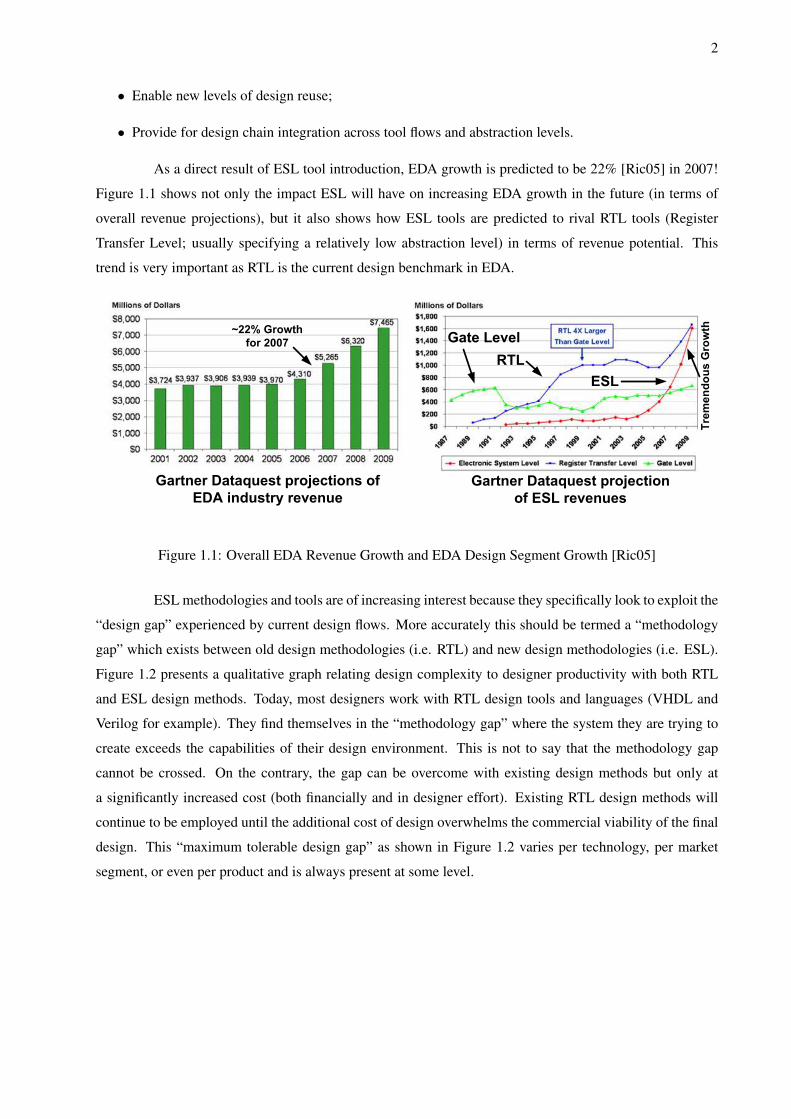
As a direct result of ESL tool introduction, EDA growth is predicted to be 22% [Ric05] in 2007!
Figure 1.1 shows not only the impact ESL will have on increasing EDA growth in the future (in terms of
overall revenue projections), but it also shows how ESL tools are predicted to rival RTL tools (Register
Transfer Level; usually specifying a relatively low abstraction level) in terms of revenue potential. This
trend is very important as RTL is the current design benchmark in EDA.
Gartner Dataquest projections of
EDA industry revenue
Gartner Dataquest projection
of ESL revenues
Gate Level
RTL
ESL
~22% Growth
for 2007
Tremendous Growth
Figure 1.1: Overall EDA Revenue Growth and EDA Design Segment Growth [Ric05]
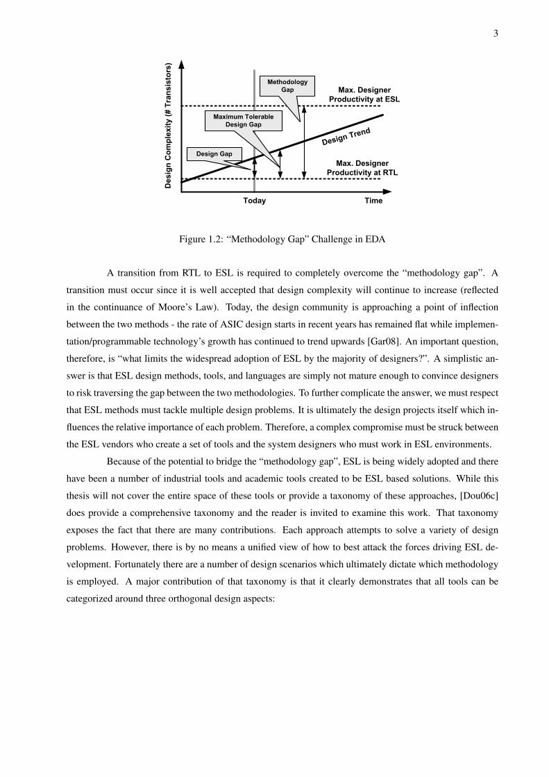
ESL methodologies and tools are of increasing interest because they specifically look to exploit the
“design gap” experienced by current design flows. More accurately this should be termed a “methodology
gap” which exists between old design methodologies (i.e. RTL) and new design methodologies (i.e. ESL).
Figure 1.2 presents a qualitative graph relating design complexity to designer productivity with both RTL
and ESL design methods. Today, most designers work with RTL design tools and languages (VHDL and
Verilog for example). They find themselves in the “methodology gap” where the system they are trying to
create exceeds the capabilities of their design environment. This is not to say that the methodology gap
cannot be crossed. On the contrary, the gap can be overcome with existing design methods but only at
a significantly increased cost (both financially and in designer effort). Existing RTL design methods will
continue to be employed until the additional cost of design overwhelms the commercial viability of the final
design. This “maximum tolerable design gap” as shown in Figure 1.2 varies per technology, per market
segment, or even per product and is always present at some level.
3
Max. Designer
Productivity at ESL
Max. Designer
Productivity at RTLD
esig
n C
om
ple
xity (# T
ransis
tors
)
TimeToday
Design Gap
Maximum Tolerable
Design Gap
Methodology
Gap
Design Trend
Figure 1.2: “Methodology Gap” Challenge in EDA
A transition from RTL to ESL is required to completely overcome the “methodology gap”. A
transition must occur since it is well accepted that design complexity will continue to increase (reflected
in the continuance of Moore’s Law). Today, the design community is approaching a point of inflection
between the two methods - the rate of ASIC design starts in recent years has remained flat while implemen-
tation/programmable technology’s growth has continued to trend upwards [Gar08]. An important question,
therefore, is “what limits the widespread adoption of ESL by the majority of designers?”. A simplistic an-
swer is that ESL design methods, tools, and languages are simply not mature enough to convince designers
to risk traversing the gap between the two methodologies. To further complicate the answer, we must respect
that ESL methods must tackle multiple design problems. It is ultimately the design projects itself which in-
fluences the relative importance of each problem. Therefore, a complex compromise must be struck between
the ESL vendors who create a set of tools and the system designers who must work in ESL environments.
Because of the potential to bridge the “methodology gap”, ESL is being widely adopted and there
have been a number of industrial tools and academic tools created to be ESL based solutions. While this
thesis will not cover the entire space of these tools or provide a taxonomy of these approaches, [Dou06c]
does provide a comprehensive taxonomy and the reader is invited to examine this work. That taxonomy
exposes the fact that there are many contributions. Each approach attempts to solve a variety of design
problems. However, there is by no means a unified view of how to best attack the forces driving ESL de-
velopment. Fortunately there are a number of design scenarios which ultimately dictate which methodology
is employed. A major contribution of that taxonomy is that it clearly demonstrates that all tools can be
categorized around three orthogonal design aspects:
4
Definition 1.0.1 Functionality - this is “what” a system does. This can also be considered the application
the design implements. Other common terms for this area are application domain or behavior.
Definition 1.0.2 Architecture - this is “how” a system carries out its operation. This can also be consid-
ered the services the system provides. Other terms for this area are platform components or services. Note
that this can be traditional HW ASIC components, programmable processing engines, as well as general
purpose processors (GPPs) capable of running software. All of this development is subject to abstraction in
which case architecture services could be anything from logic gates to ISA instructions. The development
of architecture service models in this area is the focus of this thesis.
Definition 1.0.3 Mapping - this is the process of assigning functionality to architecture (behavior to ser-
vices). Often this is called binding as well and is traditionally seen as part of the synthesis process. This
an assignment between behaviors in the functional model and services in the architectural model. Mapping
can be “many-to-one”. This allows “many” functional behaviors to be assigned to “one” architectural
service. For example a DCT and FFT behavior can be mapped to a single abstract service dealing with
signal processing.
There is a great deal of work related to each of these three areas as was shown in the taxonomy
work [Dou06c]. Often ESL tools will fall into one of these categories only or perhaps combinations. The
areas themselves will be touched on more specifically in Section 1.2 when System Level Design (a method-
ology within ESL) is described in more depth. It should be pointed out again that this thesis in general will
focus on architecture service model development for ESL. This thesis will demonstrate how embedded
system architecture service models can be created and how to formally verify properties of these models as
it relates to refinement.
At this point is should be made very clear that this work is of interest since in order to legitimize
ESL and to continue its adoption, architecture service modeling will need to be provided in such a way that
various desired ESL characteristics attributed to abstraction can be maintained while achieving performance
goals associated with RTL. Specifically this thesis will:
Demonstrate that architecture service modeling in system level design (SLD) can allow abstraction and
modularity while maintaining accuracy and efficiency.
Abstraction allows the system to be described early and at a reasonable cost but it also casts a
shadow of doubt over the accuracy of performance analysis data. Since the data gathered during simu-
lation guide the selection of one system architecture over another, the veracity of data recovered from ESL
5
performance analysis techniques with respect to the system feature being investigated must be considered
carefully by the designer. Fear of inaccuracy in ESL performance analysis is a major impediment to the tran-
sition from RTL to ESL. Preventing this inaccuracy is paramount for ESL acceptance and legitimacy
and is the major goal of this thesis.
Modularity encourages reuse, localizes system functionality, provides more system observability,
and helps to manage complex system development. However modularity can often be at odds with sim-
ulation efficiency. Overheads often associated with modularity may decrease simulation speed or enforce
rigid syntactic or semantic requirements on the designer. If a design environment is to be widely accepted it
must remain equally efficient (if not more so) as the current design environments it is replacing for the same
amount of design productivity gains (both in terms of design time saved and design space explored). Pre-
venting this inefficiency is also paramount for ESL acceptance and legitimacy and is partner to accuracy
as a goal of this thesis.
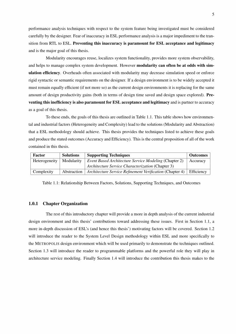
To these ends, the goals of this thesis are outlined in Table 1.1. This table shows how environmen-
tal and industrial factors (Heterogeneity and Complexity) lead to the solutions (Modularity and Abstraction)
that a ESL methodology should achieve. This thesis provides the techniques listed to achieve these goals
and produce the stated outcomes (Accuracy and Efficiency). This is the central proposition of all of the work
contained in this thesis.
Factor Solutions Supporting Techniques OutcomesHeterogeneity Modularity Event Based Architecture Service Modeling (Chapter 2) Accuracy
Architecture Service Characterization (Chapter 3)Complexity Abstraction Architecture Service Refinement Verification (Chapter 4) Efficiency
Table 1.1: Relationship Between Factors, Solutions, Supporting Techniques, and Outcomes
1.0.1 Chapter Organization
The rest of this introductory chapter will provide a more in depth analysis of the current industrial
design environment and this thesis’ contributions toward addressing these issues. First in Section 1.1, a
more in-depth discussion of ESL’s (and hence this thesis’) motivating factors will be covered. Section 1.2
will introduce the reader to the System Level Design methodology within ESL and more specifically to
the METROPOLIS design environment which will be used primarily to demonstrate the techniques outlined.
Section 1.3 will introduce the reader to programmable platforms and the powerful role they will play in
architecture service modeling. Finally Section 1.4 will introduce the contribution this thesis makes to the
6
area of ESL in the form of a complete design flow. It will outline a naıve design flow approach and close
the chapter with the improved proposed design flow which will be discussed throughout this thesis.
1.1 Motivating Factors
There is a great deal of financial commitment and human resource effort involved in EDA. In
2005 the revenue in EDA was 3.9 billion dollars and was 4.3 billion dollars in 2006. It is projected as
being as high as 7.4 billion dollars in 2009 [Ric05]. According to [Rav05] the embedded hardware market
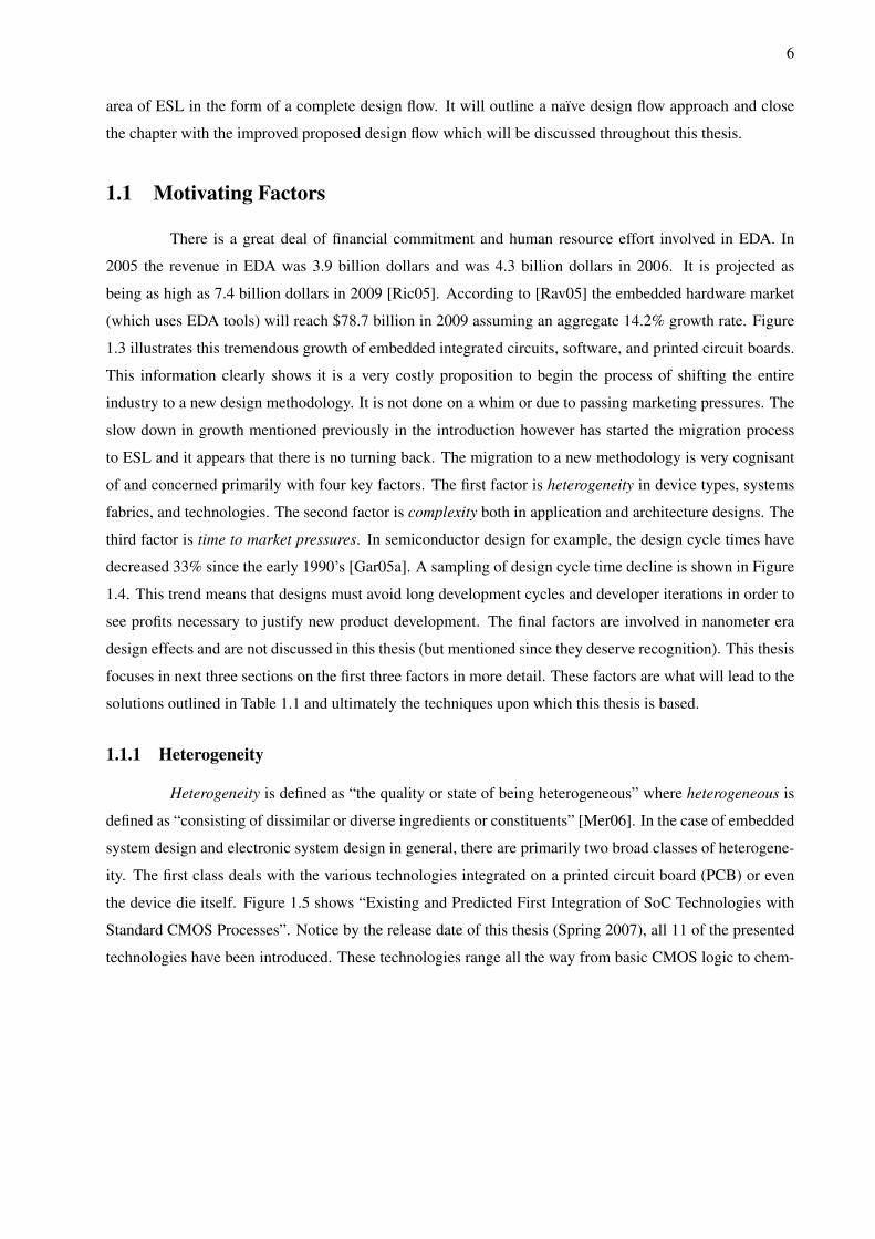
(which uses EDA tools) will reach $78.7 billion in 2009 assuming an aggregate 14.2% growth rate. Figure
1.3 illustrates this tremendous growth of embedded integrated circuits, software, and printed circuit boards.
This information clearly shows it is a very costly proposition to begin the process of shifting the entire
industry to a new design methodology. It is not done on a whim or due to passing marketing pressures. The
slow down in growth mentioned previously in the introduction however has started the migration process
to ESL and it appears that there is no turning back. The migration to a new methodology is very cognisant
of and concerned primarily with four key factors. The first factor is heterogeneity in device types, systems
fabrics, and technologies. The second factor is complexity both in application and architecture designs. The
third factor is time to market pressures. In semiconductor design for example, the design cycle times have
decreased 33% since the early 1990’s [Gar05a]. A sampling of design cycle time decline is shown in Figure
1.4. This trend means that designs must avoid long development cycles and developer iterations in order to
see profits necessary to justify new product development. The final factors are involved in nanometer era
design effects and are not discussed in this thesis (but mentioned since they deserve recognition). This thesis
focuses in next three sections on the first three factors in more detail. These factors are what will lead to the
solutions outlined in Table 1.1 and ultimately the techniques upon which this thesis is based.
1.1.1 Heterogeneity
Heterogeneity is defined as “the quality or state of being heterogeneous” where heterogeneous is
defined as “consisting of dissimilar or diverse ingredients or constituents” [Mer06]. In the case of embedded
system design and electronic system design in general, there are primarily two broad classes of heterogene-
ity. The first class deals with the various technologies integrated on a printed circuit board (PCB) or even
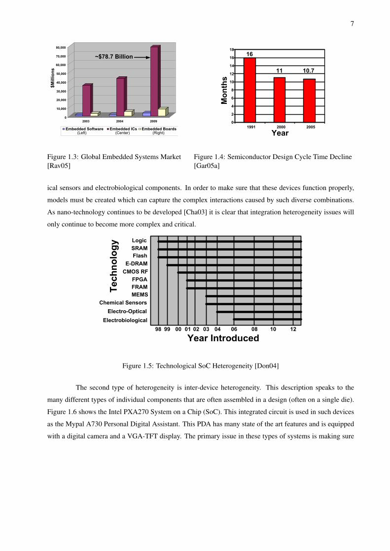
the device die itself. Figure 1.5 shows “Existing and Predicted First Integration of SoC Technologies with
Standard CMOS Processes”. Notice by the release date of this thesis (Spring 2007), all 11 of the presented
technologies have been introduced. These technologies range all the way from basic CMOS logic to chem-
7
0
10,000
20,000
30,000
40,000
50,000
60,000
70,000
80,000
2003 2004 2009
Embedded Software Embedded ICs Embedded Boards
$M
illi
on
s
~$78.7 Billion
(Left) (Center) (Right)
Figure 1.3: Global Embedded Systems Market[Rav05]
0
2
4
6
8
10
12
14
16
18
1991 2000 2005
16
11 10.7
Figure 1.4: Semiconductor Design Cycle Time Decline[Gar05a]
ical sensors and electrobiological components. In order to make sure that these devices function properly,
models must be created which can capture the complex interactions caused by such diverse combinations.
As nano-technology continues to be developed [Cha03] it is clear that integration heterogeneity issues will
only continue to become more complex and critical.
Logic
SRAM
Flash
E-DRAM
CMOS RF
FPGA
FRAM
MEMS
Chemical Sensors
Electro-Optical
Electrobiological
98 99 00 01 02 03 04 06 08 10 12
Figure 1.5: Technological SoC Heterogeneity [Don04]
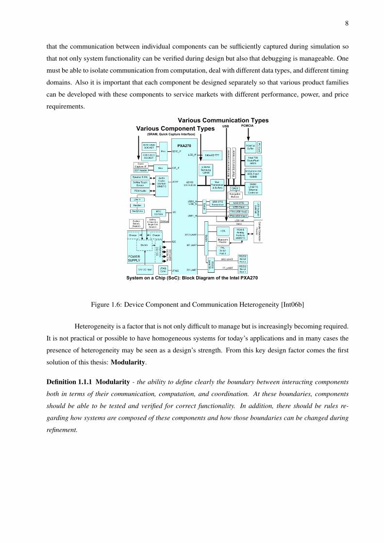
The second type of heterogeneity is inter-device heterogeneity. This description speaks to the
many different types of individual components that are often assembled in a design (often on a single die).
Figure 1.6 shows the Intel PXA270 System on a Chip (SoC). This integrated circuit is used in such devices
as the Mypal A730 Personal Digital Assistant. This PDA has many state of the art features and is equipped
with a digital camera and a VGA-TFT display. The primary issue in these types of systems is making sure
8
that the communication between individual components can be sufficiently captured during simulation so
that not only system functionality can be verified during design but also that debugging is manageable. One
must be able to isolate communication from computation, deal with different data types, and different timing
domains. Also it is important that each component be designed separately so that various product families
can be developed with these components to service markets with different performance, power, and price
requirements.
System on a Chip (SoC): Block Diagram of the Intel PXA270
PCMCIAUSB
System Bus
(SRAM, Quick Capture Interface)
Figure 1.6: Device Component and Communication Heterogeneity [Int06b]
Heterogeneity is a factor that is not only difficult to manage but is increasingly becoming required.
It is not practical or possible to have homogeneous systems for today’s applications and in many cases the
presence of heterogeneity may be seen as a design’s strength. From this key design factor comes the first
solution of this thesis: Modularity.
Definition 1.1.1 Modularity - the ability to define clearly the boundary between interacting components
both in terms of their communication, computation, and coordination. At these boundaries, components
should be able to be tested and verified for correct functionality. In addition, there should be rules re-
garding how systems are composed of these components and how those boundaries can be changed during
refinement.
9
If a design is modular, one can test its components in isolation and will allow for reuse. Modu-
larity allows communication issues to be isolated from computation issues as well. Throughout this thesis,
modularity will be emphasized as it is a critical contribution in the design of system level architecture
service simulation and verification techniques. Modularity will be constantly monitored in the context of
maintaining an efficient simulation environment.
1.1.2 Complexity
The second factor influencing the development of system level design methodologies is the in-
creasing complexity seen both at the application level as well as how many devices can be introduced on
a die. Moores law fuels much of this progress on the technology side but applications are increasingly
requiring more memory and compute power. Multimedia applications are an excellent example of this phe-
nomenon. IBM’s cell processor [Jim05] (an example of a cutting edge architecture design) is prominently
featured in the Sony Playstation 3 and the most sophisticated devices in PCs today are related to graphics
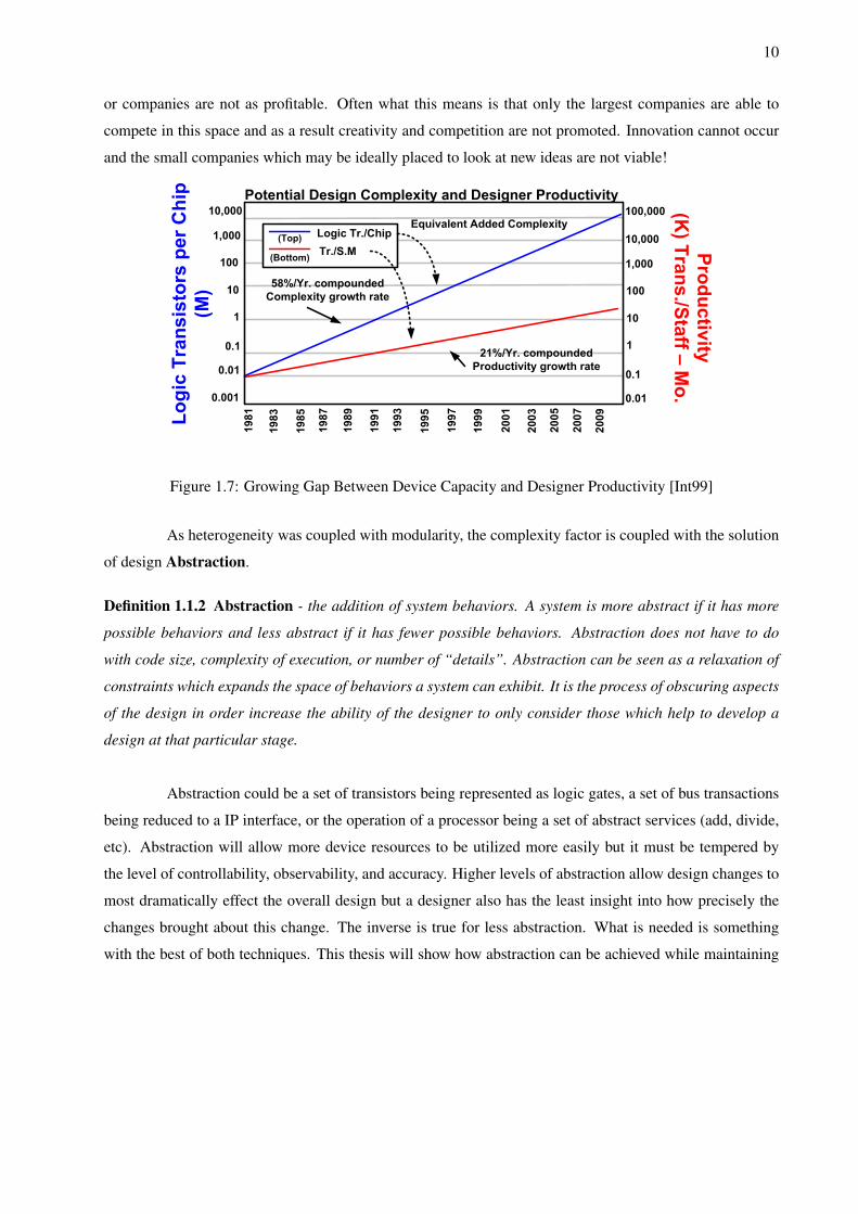
processing for videogames [Nol05]. Figure 1.7 provides a very clear illustration of the issues these com-
plexity trends introduce. One of these is the increasing complexity of designs as measured by the number
of transistors present in a device. This figure shows a 58% per year compounded complexity growth rate.
However, the productivity rate (as measured in transistors per staff month) is only increasing at a 21% com-
pounded growth rate. This growth rate mismatch leads to an increasing productivity gap (this manifests
itself as the “methodology gap” discussed earlier). There is no inherent problem with the producvity gap.
In theory this just means that all of the power of a device will not be realized. However in practice this gap
leads to at least two side effects. The first effect is that in the quest to utilze all that complexity, designs end
up taking more time to develop. This is due to the fact that new architectural innovations must occur in order
to take advantage of the added silicon. In the case of general purpose processors for example, companies
like Intel are no longer pursuing advanced superscalar techniques but rather looking a multi- and many-core
devices. These designs bring with them a whole set of verfication, test, and design difficulties. In the event
that productitvity can not keep pace it is very likely that design times will dramatically increase. This trans-
lates into lost revenue and lost opportunities for many companies. In order to prevent this, the second effect
is seen. Companies often respond by increasing the number of employees to tackle this problem. This leads
to more development costs which end up raising the cost of the device. It is also not clear that this is simply
a manpower issue. It is possible that more manpower will only exacerbate the complexity and management
problem. In the event that the market will not bare this increased cost either the employees cannot be hired
10
or companies are not as profitable. Often what this means is that only the largest companies are able to
compete in this space and as a result creativity and competition are not promoted. Innovation cannot occur
and the small companies which may be ideally placed to look at new ideas are not viable!
10,000
1,000
100
10
1
0.1
0.01
0.001
Potential Design Complexity and Designer Productivity100,000
10,000
1,000
100
10
1
0.1
0.01
1981
1983
1985
1987
1989
1991
1993
1997
1999
2001
2003
2005
2007
2009
1995
Equivalent Added Complexity
58%/Yr. compounded
Complexity growth rate
21%/Yr. compounded
Productivity growth rate
(Top)
(Bottom)
Logic Tr./Chip
Tr./S.M
Figure 1.7: Growing Gap Between Device Capacity and Designer Productivity [Int99]
As heterogeneity was coupled with modularity, the complexity factor is coupled with the solution
of design Abstraction.
Definition 1.1.2 Abstraction - the addition of system behaviors. A system is more abstract if it has more
possible behaviors and less abstract if it has fewer possible behaviors. Abstraction does not have to do
with code size, complexity of execution, or number of “details”. Abstraction can be seen as a relaxation of
constraints which expands the space of behaviors a system can exhibit. It is the process of obscuring aspects
of the design in order increase the ability of the designer to only consider those which help to develop a
design at that particular stage.
Abstraction could be a set of transistors being represented as logic gates, a set of bus transactions
being reduced to a IP interface, or the operation of a processor being a set of abstract services (add, divide,
etc). Abstraction will allow more device resources to be utilized more easily but it must be tempered by
the level of controllability, observability, and accuracy. Higher levels of abstraction allow design changes to
most dramatically effect the overall design but a designer also has the least insight into how precisely the
changes brought about this change. The inverse is true for less abstraction. What is needed is something
with the best of both techniques. This thesis will show how abstraction can be achieved while maintaining
11
accuracy. Specifically maintaining relative accuracy or fidelity.
Definition 1.1.3 Fidelity - requires that all pairs of corresponding measurements m1, m2 in a abstract
model and p1, p2 on the actual implementation, hold m1 < m2 if and only if p1 < p2.
1.1.3 Time to Market
The first two factors, heterogeneity and complexity, were aspects of embedded system designs
that were technology and application driven. The final factor, time to market pressure, is consumer driven
and is in opposition to the other factors. Time to market is why a design method needs to be accurate and
efficient. If it is not, there will be long iterations in the design and as a consequence release dates will slip.
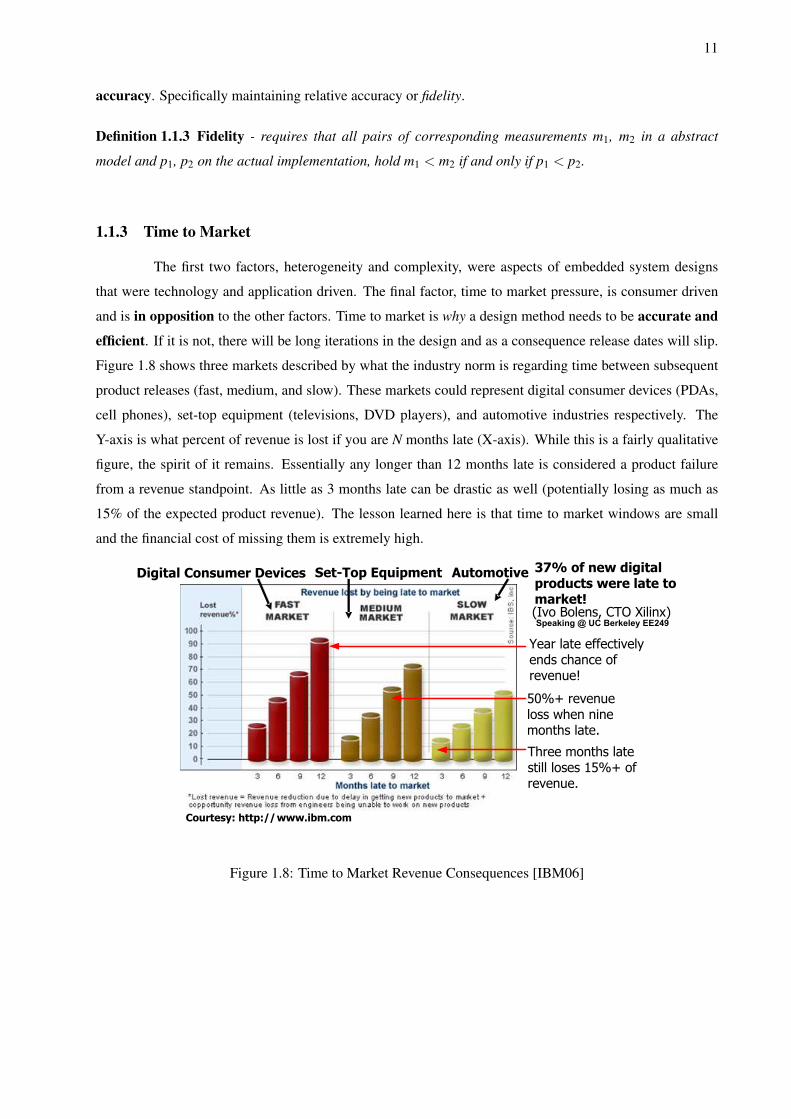
Figure 1.8 shows three markets described by what the industry norm is regarding time between subsequent
product releases (fast, medium, and slow). These markets could represent digital consumer devices (PDAs,
cell phones), set-top equipment (televisions, DVD players), and automotive industries respectively. The
Y-axis is what percent of revenue is lost if you are N months late (X-axis). While this is a fairly qualitative
figure, the spirit of it remains. Essentially any longer than 12 months late is considered a product failure
from a revenue standpoint. As little as 3 months late can be drastic as well (potentially losing as much as
15% of the expected product revenue). The lesson learned here is that time to market windows are small
and the financial cost of missing them is extremely high.
Courtesy: http://www.ibm.com
Year late effectively ends chance of revenue!
50%+ revenue loss when nine months late.
Three months late still loses 15%+ of revenue.
37% of new digital products were late to market!
Digital Consumer Devices Set-Top Equipment Automotive
(Ivo Bolens, CTO Xilinx)Speaking @ UC Berkeley EE249
Figure 1.8: Time to Market Revenue Consequences [IBM06]
12
Time to market issues cannot be ignored since it they are why companies cannot take an arbitrary
amount of time to produce designs. Granted it is not the only factor calling for an efficient design process (for
example it would not be cost effective to manufacture an arbitrary number of devices at any design process
speed in order to weed out process errors) but it is nonetheless a very powerful factor and the underlying
influence behind almost all EDA efforts (tool design by nature looks to speed up the design process since
time is often equated with designer effort).
1.2 1st Focus: System Level Design
The beginning of this chapter discussed Electronic System Level (ESL) design and its increasingly
important role in EDA. Often an approach within ESL concerned with specific system wide integration goals
(reuse, modularity, formal techniques) is called System Level Design (SLD) [Kur00] (often ESL and SLD
are used interchangeably). SLD allows for a designer to think of traditional software and hardware aspects
of the design separately. Algorithms are decoupled from the elements which implement them. For the
purposes of this thesis, system level design is going to refer primarily to the level of abstraction employed.
Computation will take place at the granularity of function calls typically. Communication operations will
be considered as transactions (as opposed to bit-level or register interactions).
Definition 1.2.1 System Level Design - a design methodology whereby the interactions amongst compo-
nents at an increased abstraction level are examined. Design is done taking the entire system into consider-
ation as well, not just individual components.
It is important to understand that SLD is a large design umbrella defined by a generic set of goals
with a number of various approaches possible within ESL. In fact within ESL there are many industrial
and academic offerings with claims to be members of the SLD community. In [Dou06c] (the taxonomy
previously mentioned), over 90 tools and environments were categorized. The approaches differed by their
ability to support (F)unctional modeling, (P)latform services, or (M)apping capabilities. Approaches could
be combinations of these distinctions. If this thesis work is to use the terminology used in that source, then
specifically it will examine an FPM approach. FPM approaches are attractive since this thesis investigation
could be carried out in one unified environment. In particular this thesis will be focusing in on a particular
style within ESL called, Platform-Based Design [Alb02]. Platform-Based Design (PBD) is concerned with
what is termed the orthogonalization of concerns. These concerns are:
• Functionality (what something does) and Architecture (how it does it). For example multiplication
13
itself is very well defined functionally. However, the architecture which implements it may be a
series of adders or a dedicated multiplier. This separation goal is shared by a variety of other SLD
methodologies.
• Behavior (Semantics) and Performance Indices (Latency, Throughput, etc). Behavior defines how a
device operates. A bus protocol is an example of a behavior. Performance is a cost of that behav-
ior. Bus transaction latency times (performance) are a function of many things not specified by the
behavior (for example clock speed is not a behavior).
• Computation, Communication, Coordination. How things compute should be separate from how they
interact (communicate) with other aspects of the system, and both computation and communication
should be separate from the scheduling mechanisms.
By keeping these issues separate, the now modular design allows for a smoother verification
process, reuse, and abstraction. These are exactly elements that were stated as goals of this thesis!
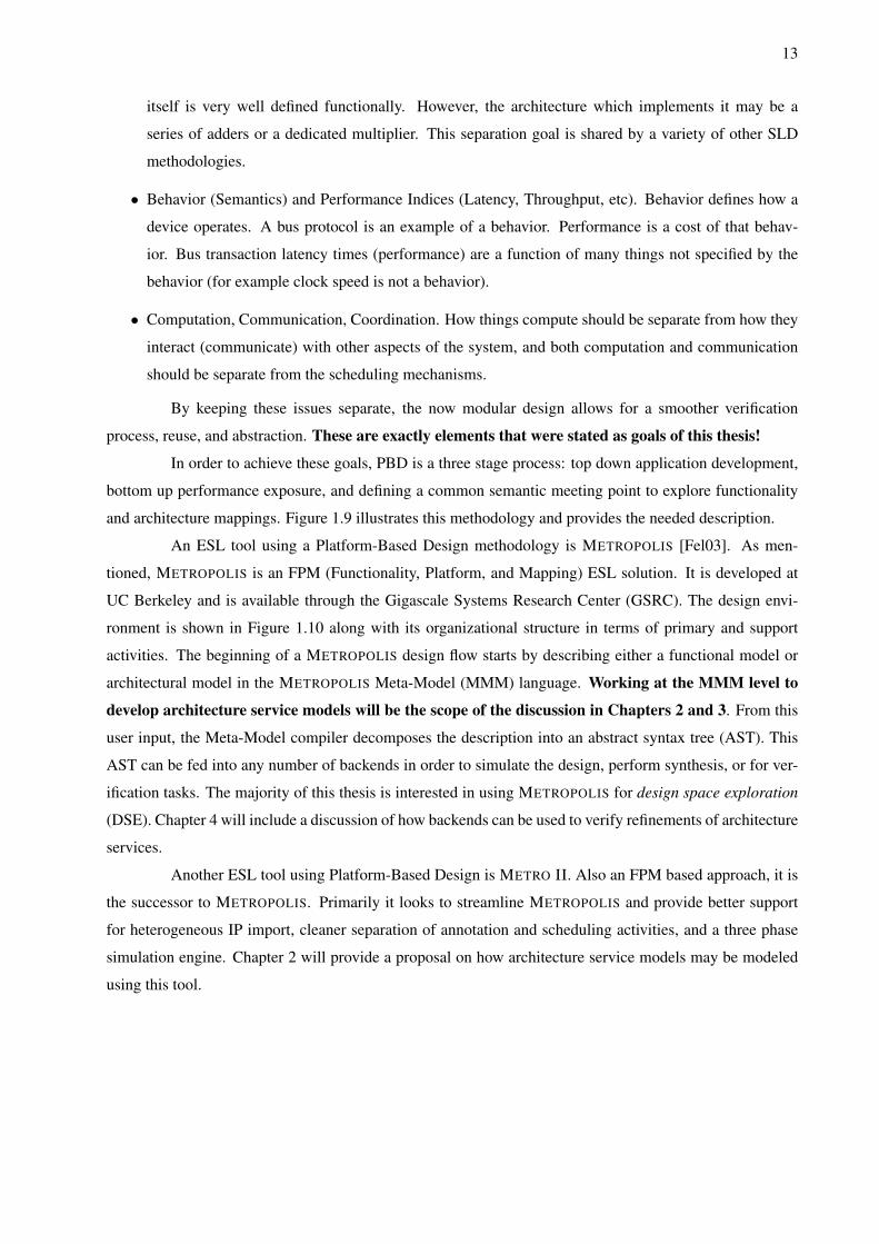
In order to achieve these goals, PBD is a three stage process: top down application development,
bottom up performance exposure, and defining a common semantic meeting point to explore functionality
and architecture mappings. Figure 1.9 illustrates this methodology and provides the needed description.
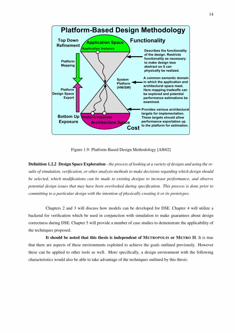
An ESL tool using a Platform-Based Design methodology is METROPOLIS [Fel03]. As men-
tioned, METROPOLIS is an FPM (Functionality, Platform, and Mapping) ESL solution. It is developed at
UC Berkeley and is available through the Gigascale Systems Research Center (GSRC). The design envi-
ronment is shown in Figure 1.10 along with its organizational structure in terms of primary and support
activities. The beginning of a METROPOLIS design flow starts by describing either a functional model or
architectural model in the METROPOLIS Meta-Model (MMM) language. Working at the MMM level to
develop architecture service models will be the scope of the discussion in Chapters 2 and 3. From this
user input, the Meta-Model compiler decomposes the description into an abstract syntax tree (AST). This
AST can be fed into any number of backends in order to simulate the design, perform synthesis, or for ver-
ification tasks. The majority of this thesis is interested in using METROPOLIS for design space exploration
(DSE). Chapter 4 will include a discussion of how backends can be used to verify refinements of architecture
services.
Another ESL tool using Platform-Based Design is METRO II. Also an FPM based approach, it is
the successor to METROPOLIS. Primarily it looks to streamline METROPOLIS and provide better support
for heterogeneous IP import, cleaner separation of annotation and scheduling activities, and a three phase
simulation engine. Chapter 2 will provide a proposal on how architecture service models may be modeled
using this tool.
14
Describes the functionality
of the design. Restricts
functionality as necessary
to make design less
abstract so it can
physically be realized.
Provides various architectural
targets for implementation.
These targets should allow
performance exportation up
to the platform for estimation.
A common semantic domain
in which the application and
architectural space meet.
Here mapping tradeoffs can
be explored and potential
performance estimations be
examined.
Top Down
Refinement
Bottom Up
Exposure
Platform
Mapping
Platform
Design Space
Export
System
Platform
(HW/SW)
Application Instance
Platform Instances
Application Space
Architecture Space
Figure 1.9: Platform-Based Design Methodology [Alb02]
Definition 1.2.2 Design Space Exploration - the process of looking at a variety of designs and using the re-
sults of simulation, verification, or other analysis methods to make decisions regarding which design should
be selected, which modifications can be made to existing designs to increase performance, and observe
potential design issues that may have been overlooked during specification. This process is done prior to
committing to a particular design with the intention of physically creating it or its prototypes.
Chapters 2 and 3 will discuss how models can be developed for DSE. Chapter 4 will utilize a
backend for verification which be used in conjunction with simulation to make guarantees about design
correctness during DSE. Chapter 5 will provide a number of case studies to demonstrate the applicability of
the techniques proposed.
It should be noted that this thesis is independent of METROPOLIS or METRO II. It is true
that there are aspects of these environments exploited to achieve the goals outlined previously. However
these can be applied to other tools as well. More specifically, a design environment with the following
characteristics would also be able to take advantage of the techniques outlined by this thesis:
15
1. Support for multiple models of computation - this thesis requires both tagged signal modeling seman-
tics as well as data flow modeling.
2. Explicitly separate an architecture model’s behavior and how its operation is scheduled - this thesis
requires this separation to meet its performance and reuse goals. The refinement formulation is also
highly dependent on this distinction.
3. Event based synchronization - this thesis requires that elements which form architecture services be
coordinated with events.
More specifics about METROPOLIS and METRO II execution and modeling will be covered in
Chapter 2 and can be found in [Fel03] and [Abh07].
1. Architecture
Service Modeling:
Chapters 2 and 3
2. Refinement
Verification:
Chapter 4
Mapping ArchitectureFunctioality
Leadership
SupportSimulationVerification
Meta Model Language
Meta Model
ComplierFront End
Back End 1 Back End NBack End 3Back End 2
Abstract Syntax Trees
Simulator
Tool Verification
Tool
Synthesis
Tool
3. Simulation
is the focus of
all the work:
Case Studies
in Chapter 5
Major Activities
Support Activities
Figure 1.10: METROPOLIS Design Environment and Organization
1.3 2nd Focus: Programmable Architecture Services
When having a discussion about creating abstract, modular architecture service models which
are still efficient and accurate one must quickly determine what types of implementation devices one is
going to consider. One could consider static architecture service models. A static architecture service model
for the purposes of this thesis is one which has its functionality bound during manufacturing. This is the
case when speaking about a General Purpose Processors (GPP) such as Intel’s Pentium 4 [Int06a] or ARM
16
style processor [ARM06]. ASIC designs could also be members of this group. These devices are perhaps
programmable at the ISA level (GPPs) but one cannot change the computation fabric or interaction between
computation or communication units after fabrication. The are usually either very special purpose (ASICs)
or very generic (GPPs). Often they have a high design cost but are often cheaper to manufacture and recoup
that design cost in sales volume. At the other end of the spectrum are programmable architectures or plat-
forms (the term platform denoting a set of services which typically are not associated with traditional CPU
architectures). A programmable platform is a system for implementing an electronic design. Examples of
these are Platform FPGAs and ASIPs. These systems are distinguished by their ability to be programmed
regarding their computation (functionality), communication (topology), or coordination (scheduling). Pro-
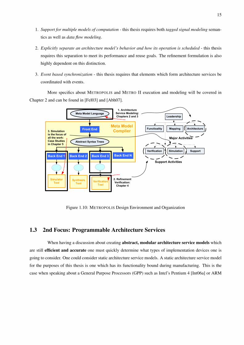
grammable platforms are increasing in use and popularity for several reasons: [Kur02], [And00]
• Rapid Time-to-Market - One can often eliminate fabrication time by using off the shelf parts. This
also bypasses a large part of the verification time as well since parts are well understood and there is
no post silicon verification phase.
• Versatility, Flexibility (increase product lifespan) - Design reuse within a programmable architecture
family is often possible.
• In-Field Upgradeability - Many devices are reprogrammable using as little as a personal computer
or a portable flash memory card.
• Performance: 2-100x compared to GPPs - Special purpose computation units can exploit spatial
concurrency or dedicated hardware can be created.
Table 1.2 lists a set of characteristics that allow programmable platforms to achieve those advan-
tages. However they naturally have some disadvantages as well:
• Performance: 2-6x slower than ASICs - Programmable architecture topology overhead related to
programming the device may hurt performance. For example, FPGAs are unable to perform routing
as efficiently as a custom ASIC due to its mesh like structure.
• Power: 13x compared to ASICs - Programmable architecture fabric is not typically optimized for
power although companies are starting to improve their power consumption dramatically.
Overall the strengths outweigh the weakness as both of the weaknesses are becoming less of an
issue as technologies mature. Programmable Platforms often have a very regular device fabrics (FPGAs for
example are famous for this). This regularity allows for advances in device technology (such as transistor
17
scaling) to be taken advantage of with minimal design changes. An FPGA is able to double its computing
capacity every 18 months with the same die size potentially. In fact, industry luminary Tsugio Makimoto of
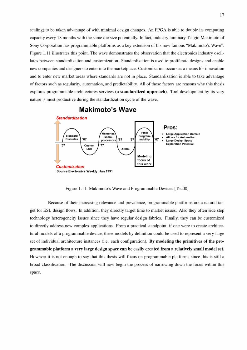
Sony Corporation has programmable platforms as a key extension of his now famous “Makimoto’s Wave”.
Figure 1.11 illustrates this point. The wave demonstrates the observation that the electronics industry oscil-
lates between standardization and customization. Standardization is used to proliferate designs and enable
new companies and designers to enter into the marketplace. Customization occurs as a means for innovation
and to enter new market areas where standards are not in place. Standardization is able to take advantage
of factors such as regularity, automation, and predictability. All of those factors are reasons why this thesis
explores programmable architectures services (a standardized approach). Tool development by its very
nature is most productive during the standardization cycle of the wave.
Modeling
focus of
this work
Large Application Domain
Allows for Automation
Large Design Space
Exploration Potential
Customization
Standardization
Source Electronics Weekly, Jan 1991
Standard
Discretes
Custom
LSIs
Memories,
Micro-
processors
ASICs
Field
Program-
mability
‘57
‘67
‘77
‘87 ‘97 ‘07
Figure 1.11: Makimoto’s Wave and Programmable Devices [Tsu00]
Because of their increasing relevance and prevalence, programmable platforms are a natural tar-
get for ESL design flows. In addition, they directly target time to market issues. Also they often side step
technology heterogeneity issues since they have regular design fabrics. Finally, they can be customized
to directly address new complex applications. From a practical standpoint, if one were to create architec-
tural models of a programmable device, these models by definition could be used to represent a very large
set of individual architecture instances (i.e. each configuration). By modeling the primitives of the pro-
grammable platform a very large design space can be easily created from a relatively small model set.
However it is not enough to say that this thesis will focus on programmable platforms since this is still a
broad classification. The discussion will now begin the process of narrowing down the focus within this
space.
18
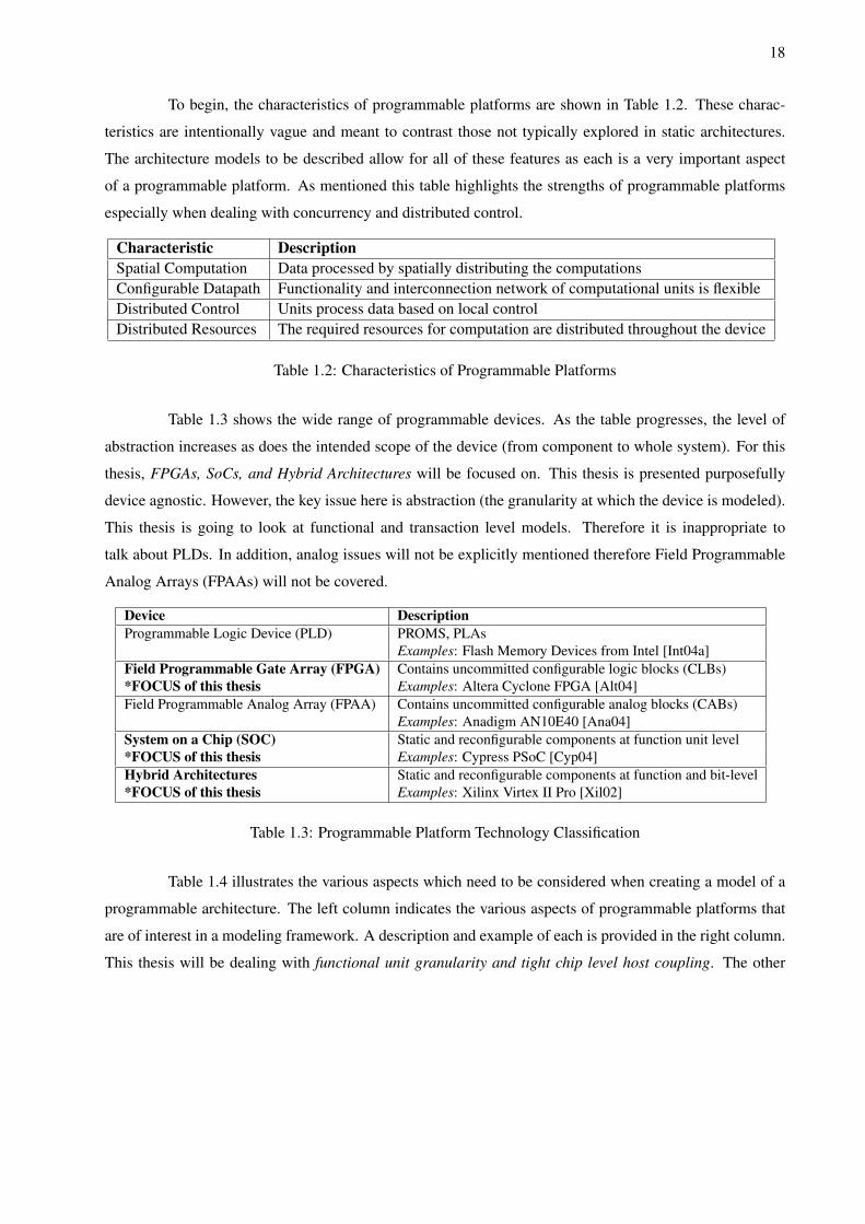
To begin, the characteristics of programmable platforms are shown in Table 1.2. These charac-
teristics are intentionally vague and meant to contrast those not typically explored in static architectures.
The architecture models to be described allow for all of these features as each is a very important aspect
of a programmable platform. As mentioned this table highlights the strengths of programmable platforms
especially when dealing with concurrency and distributed control.
Characteristic DescriptionSpatial Computation Data processed by spatially distributing the computationsConfigurable Datapath Functionality and interconnection network of computational units is flexibleDistributed Control Units process data based on local controlDistributed Resources The required resources for computation are distributed throughout the device
Table 1.2: Characteristics of Programmable Platforms
Table 1.3 shows the wide range of programmable devices. As the table progresses, the level of
abstraction increases as does the intended scope of the device (from component to whole system). For this
thesis, FPGAs, SoCs, and Hybrid Architectures will be focused on. This thesis is presented purposefully
device agnostic. However, the key issue here is abstraction (the granularity at which the device is modeled).
This thesis is going to look at functional and transaction level models. Therefore it is inappropriate to
talk about PLDs. In addition, analog issues will not be explicitly mentioned therefore Field Programmable
Analog Arrays (FPAAs) will not be covered.
Device DescriptionProgrammable Logic Device (PLD) PROMS, PLAs
Examples: Flash Memory Devices from Intel [Int04a]Field Programmable Gate Array (FPGA) Contains uncommitted configurable logic blocks (CLBs)*FOCUS of this thesis Examples: Altera Cyclone FPGA [Alt04]Field Programmable Analog Array (FPAA) Contains uncommitted configurable analog blocks (CABs)
Examples: Anadigm AN10E40 [Ana04]System on a Chip (SOC) Static and reconfigurable components at function unit level*FOCUS of this thesis Examples: Cypress PSoC [Cyp04]Hybrid Architectures Static and reconfigurable components at function and bit-level*FOCUS of this thesis Examples: Xilinx Virtex II Pro [Xil02]
Table 1.3: Programmable Platform Technology Classification
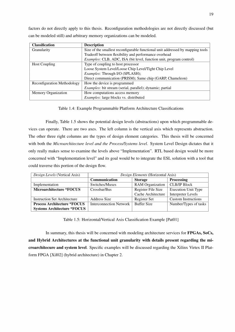
Table 1.4 illustrates the various aspects which need to be considered when creating a model of a
programmable architecture. The left column indicates the various aspects of programmable platforms that
are of interest in a modeling framework. A description and example of each is provided in the right column.
This thesis will be dealing with functional unit granularity and tight chip level host coupling. The other
19
factors do not directly apply to this thesis. Reconfiguration methodologies are not directly discussed (but
can be modeled still) and arbitrary memory organizations can be modeled.
Classification DescriptionGranularity Size of the smallest reconfigurable functional unit addressed by mapping tools
Tradeoff between flexibility and performance overheadExamples: CLB, ADC, ISA (bit level, function unit, program control)
Host Coupling Type of coupling to host processorLoose System Level/Loose Chip Level/Tight Chip LevelExamples: Through I/O (SPLASH);Direct communication (PRISM); Same chip (GARP, Chameleon)
Reconfiguration Methodology How the device is programmedExamples: bit stream (serial, parallel); dynamic; partial
Memory Organization How computations access memoryExamples: large blocks vs. distributed
Table 1.4: Example Programmable Platform Architecture Classifications
Finally, Table 1.5 shows the potential design levels (abstractions) upon which programmable de-
vices can operate. There are two axes. The left column is the vertical axis which represents abstraction.
The other three right columns are the types of design element categories. This thesis will be concerned
with both the Microarchitecture level and the Process/Systems level. System Level Design dictates that it
only really makes sense to examine the levels above “Implementation”. RTL based design would be more
concerned with “Implementation level” and its goal would be to integrate the ESL solution with a tool that
could traverse this portion of the design flow.
Design Levels (Vertical Axis) Design Elements (Horizontal Axis)Communication Storage Processing
Implementation Switches/Muxes RAM Organization CLB/IP BlockMicroarchitecture *FOCUS Crossbar/Bus Register File Size Execution Unit Type
Cache Architecture Interpreter LevelsInstruction Set Architecture Address Size Register Set Custom InstructionsProcess Architecture *FOCUS Interconnection Network Buffer Size Number/Types of tasksSystems Architecture *FOCUS
Table 1.5: Horizontal/Vertical Axis Classification Example [Pat01]
In summary, this thesis will be concerned with modeling architecture services for FPGAs, SoCs,
and Hybrid Architectures at the functional unit granularity with details present regarding the mi-
croarchitecure and system level. Specific examples will be discussed regarding the Xilinx Virtex II Plat-
form FPGA [Xil02] (hybrid architecture) in Chapter 2.
20
These sets of programmable platform categorizations were chosen since they are at the appropriate
level of abstraction desired. Additionally, they are easily described as modular components. They are easy
to characterize which will improve accuracy as well.
1.4 Thesis Contribution
At this point the reader should now be familiar with the items necessary to understand the back-
ground, goals, and context of this thesis. This final section will attempt to make very clear the contribution
of this research. Thus far this chapter has established several things:
• Introduced Heterogeneity, Complexity, and Time-to-Market pressures as the motivating factors in
this research. These factors must be addressed in order for EDA to move forward to new growth areas
and develop new methodologies for its continued success.
• Matched the design factors to the design solutions intended to resolve them (Heterogeneity to Mod-
ularity and Complexity to Abstraction).
• Identified the outcomes that are desired: Accuracy and Efficiency and the ability to meet Time-
to-Market demands. It is not enough to simply create abstract and modular designs without being
accurate and efficiency. It is clear that ESL adoption is dependent on the ability to ensure these
qualities.
• Introduced METROPOLIS and METRO II as the ESL, FPM, platform-based design approaches that
will be used to explore these concepts. In the event the one does not uses these frameworks, the
required constructs have been outlined as well.
• Identified that Programmable Platform Architectures Services are going to be the focus of the
architecture service modeling in the methodology to be described. Not only do these devices look
to address the same concerns as ESL, but they also possess key characteristics which make archi-
tecture modeling at the system level more accurate and efficient. Creating one set of programmable
components takes the place of creating a very large set of static components.
What now remains is to demonstrate how these contributions combine to create a design flow to
accomplish the desired outcomes. What will be presented next are two approaches.
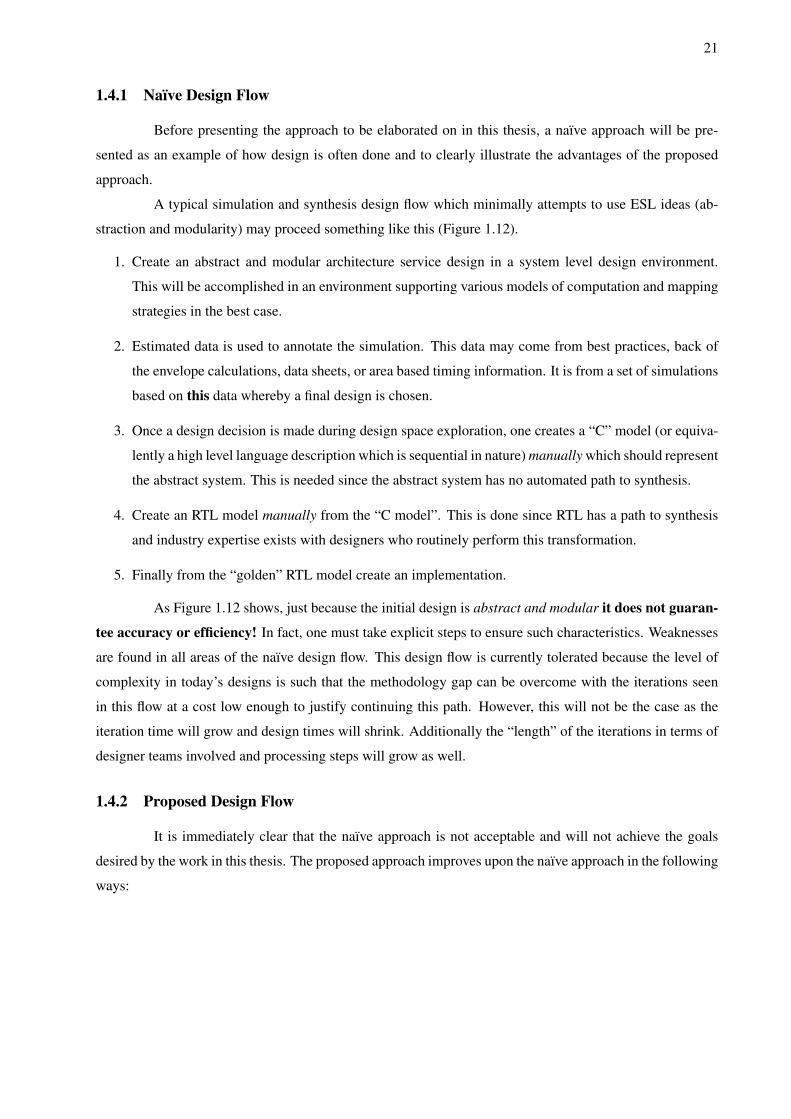
21
1.4.1 Naıve Design Flow
Before presenting the approach to be elaborated on in this thesis, a naıve approach will be pre-
sented as an example of how design is often done and to clearly illustrate the advantages of the proposed
approach.
A typical simulation and synthesis design flow which minimally attempts to use ESL ideas (ab-
straction and modularity) may proceed something like this (Figure 1.12).
1. Create an abstract and modular architecture service design in a system level design environment.
This will be accomplished in an environment supporting various models of computation and mapping
strategies in the best case.
2. Estimated data is used to annotate the simulation. This data may come from best practices, back of
the envelope calculations, data sheets, or area based timing information. It is from a set of simulations
based on this data whereby a final design is chosen.
3. Once a design decision is made during design space exploration, one creates a “C” model (or equiva-
lently a high level language description which is sequential in nature) manually which should represent
the abstract system. This is needed since the abstract system has no automated path to synthesis.
4. Create an RTL model manually from the “C model”. This is done since RTL has a path to synthesis
and industry expertise exists with designers who routinely perform this transformation.
5. Finally from the “golden” RTL model create an implementation.
As Figure 1.12 shows, just because the initial design is abstract and modular it does not guaran-
tee accuracy or efficiency! In fact, one must take explicit steps to ensure such characteristics. Weaknesses
are found in all areas of the naıve design flow. This design flow is currently tolerated because the level of
complexity in today’s designs is such that the methodology gap can be overcome with the iterations seen
in this flow at a cost low enough to justify continuing this path. However, this will not be the case as the
iteration time will grow and design times will shrink. Additionally the “length” of the iterations in terms of
designer teams involved and processing steps will grow as well.
1.4.2 Proposed Design Flow
It is immediately clear that the naıve approach is not acceptable and will not achieve the goals
desired by the work in this thesis. The proposed approach improves upon the naıve approach in the following
ways:
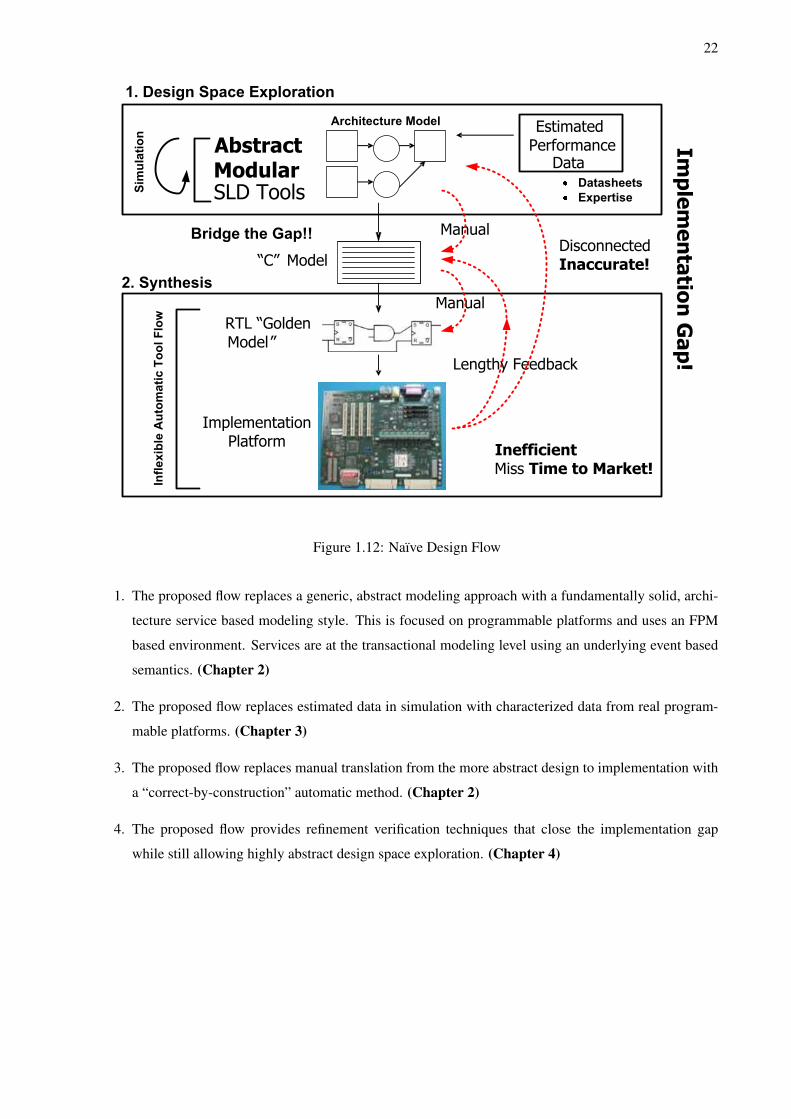
22
SLD Tools
ImplementationPlatform
RTL “Golden Model”
“C” Model
Manual
ManualDisconnectedInaccurate!
Lengthy Feedback
Inefficient
Miss Time to Market!
EstimatedPerformance
Data
Architecture Model
Datasheets
Expertise
Sim
ula
tion
2. Synthesis
Bridge the Gap!!
1. Design Space Exploration
Inflexib
le A
uto
matic T
ool Flo
w
Figure 1.12: Naıve Design Flow
1. The proposed flow replaces a generic, abstract modeling approach with a fundamentally solid, archi-
tecture service based modeling style. This is focused on programmable platforms and uses an FPM
based environment. Services are at the transactional modeling level using an underlying event based
semantics. (Chapter 2)
2. The proposed flow replaces estimated data in simulation with characterized data from real program-
mable platforms. (Chapter 3)
3. The proposed flow replaces manual translation from the more abstract design to implementation with
a “correct-by-construction” automatic method. (Chapter 2)
4. The proposed flow provides refinement verification techniques that close the implementation gap
while still allowing highly abstract design space exploration. (Chapter 4)
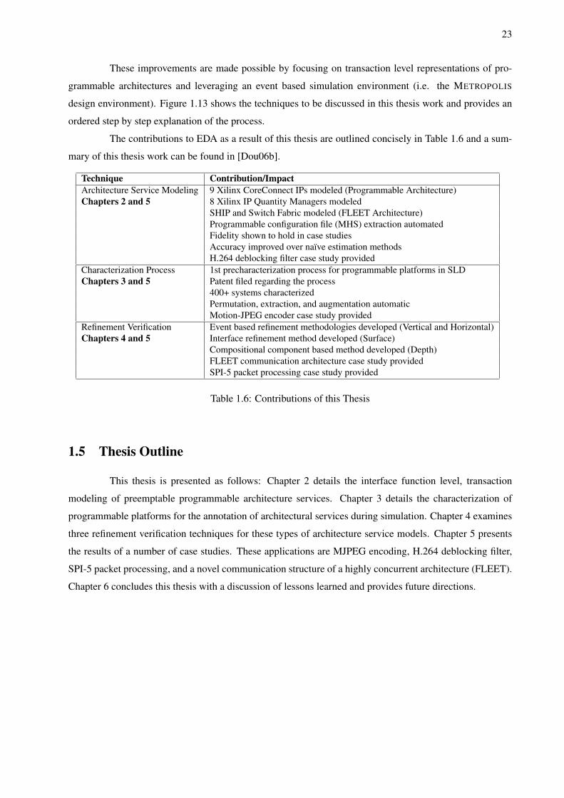
23
These improvements are made possible by focusing on transaction level representations of pro-
grammable architectures and leveraging an event based simulation environment (i.e. the METROPOLIS
design environment). Figure 1.13 shows the techniques to be discussed in this thesis work and provides an
ordered step by step explanation of the process.
The contributions to EDA as a result of this thesis are outlined concisely in Table 1.6 and a sum-
mary of this thesis work can be found in [Dou06b].
Technique Contribution/ImpactArchitecture Service Modeling 9 Xilinx CoreConnect IPs modeled (Programmable Architecture)Chapters 2 and 5 8 Xilinx IP Quantity Managers modeled
SHIP and Switch Fabric modeled (FLEET Architecture)Programmable configuration file (MHS) extraction automatedFidelity shown to hold in case studiesAccuracy improved over naıve estimation methodsH.264 deblocking filter case study provided
Characterization Process 1st precharacterization process for programmable platforms in SLDChapters 3 and 5 Patent filed regarding the process
400+ systems characterizedPermutation, extraction, and augmentation automaticMotion-JPEG encoder case study provided
Refinement Verification Event based refinement methodologies developed (Vertical and Horizontal)Chapters 4 and 5 Interface refinement method developed (Surface)
Compositional component based method developed (Depth)FLEET communication architecture case study providedSPI-5 packet processing case study provided
Table 1.6: Contributions of this Thesis
1.5 Thesis Outline
This thesis is presented as follows: Chapter 2 details the interface function level, transaction
modeling of preemptable programmable architecture services. Chapter 3 details the characterization of
programmable platforms for the annotation of architectural services during simulation. Chapter 4 examines
three refinement verification techniques for these types of architecture service models. Chapter 5 presents
the results of a number of case studies. These applications are MJPEG encoding, H.264 deblocking filter,
SPI-5 packet processing, and a novel communication structure of a highly concurrent architecture (FLEET).
Chapter 6 concludes this thesis with a discussion of lessons learned and provides future directions.
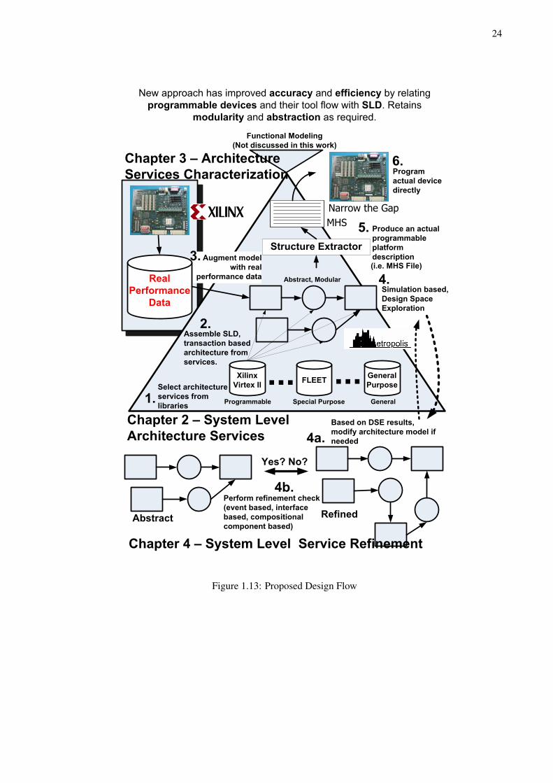
24
Xilinx
Virtex IIFLEET
General
Purpose
Real
Performance
Data
Select architecture
services from
libraries
Assemble SLD,
transaction based
architecture from
services.
Abstract, Modular
GeneralSpecial Purpose
Augment model
with real
performance data
Simulation based,
Design Space
Exploration
Structure Extractor
Produce an actual
programmable
platform
description(i.e. MHS File)
Narrow the Gap
Programmable
Functional Modeling
(Not discussed in this work)
accuracy efficiency
programmable devices SLD
modularity abstraction
Program
actual device
directly
Abstract Refined
Based on DSE results,
modify architecture model if
needed
Perform refinement check
(event based, interface
based, compositional
component based)
Yes? No?
MHS
Figure 1.13: Proposed Design Flow
25
Chapter 2
System Level Architecture Services
“Hardware: the part of the computer that can be kicked” - Jeff Pesis
Architecture service modeling is the process of creating an environment to represent and ex-
pose services that can be used to implement functionality. Services represent capabilities of the underlying
architecture upon which the design will be eventually implemented. These services are exposed to the de-
signer and a correspondence can be made between the functionality present in the application model and the
services exposed (this is a mapping). This service based environment is then used to investigate the perfor-
mances that potentially can be obtained by using collections of these systems. This methodology requires
the explicit separation of the functional model and the architecture model. This separation exists in the
Platform-Based Design methodology (described in Chapter 1) and is required throughout this thesis. This
chapter will detail the background and related work in creating architecture services of this type, provide
details of programmable service models that have been created, and outline the key features of this style of
design space exploration.
Traditionally architecture and functional models have been merged. For example, synthesizable
RTL design implicitly ties what the system does along with the physical structures that will implement it.
Other systems begin with a functional description and this description morphs into hardware and software
through a series of refinement steps. While this process can be automated, to some extent there does not exist
descriptions of the system which are purely functional or purely architectural. As a result, when a designer
wants to reuse the functional specification using a new architecture, either a new design must be written, or
minimally rolled back to the most abstract version. In any event, much design and verification work will be
lost. This thesis’ approach looks to eliminate this inefficient and potentially error prone process.
However, in the event that this functional/architecture separation does not exist, architecture mod-
eling is difficult to define, has a broad set of interpretations, and classically results in modeling structural
26
or topological details of an electronic system. Examples of these alternate styles are covered in Section
2.2 (related work). There are a number of tradeoffs possible by using these alternate styles. For this thesis
however, it is assumed that such a separation exists and the ultimate goal of the modeling effort is for de-
sign space exploration via simulation. This chapter will demonstrate why this style was chosen, how it was
implemented, and how it ultimately achieved the architecture modeling goals outlined in Chapter 1.
This chapter will illustrate how to model architecture services at the transaction level so that modularity
and accuracy will be maintained. This requires support for a variety of architecture topologies, service
exposure levels, and extensions for mapping. This process is clearly illustrated in a platform-based design
environment.
A key question which must be answered in this thesis is: “what is a service?”. It is important to
remember that architecture modeling efforts can stretch many abstraction levels. For example a basic logic
operation “A AND B” can be implemented as a 2-input AND gate or it could also be implemented as a
N-input AND gate where two of the inputs are A and B and the other N− 2 inputs are tied to “logical 1”.
In either case an AND service would be exposed but each case may have a different cost associated with it.
Another example at the other end of the abstraction spectrum is a Discreet Cosine Transform (DCT). This
operation can be carried out on a model of a general purpose processor or a dedicated HW DCT. Again each
would be a DCT service but the former may have a higher execution time cost than a dedicated HW block.
There are many different ways of modeling architectures to this end. A model can be a single entity or a
collection of smaller entities that make up a larger system. Essentially a service has an interface and a cost.
Services will be defined formally in Section 2.1 and a high level picture is shown in Figure 2.4.
Tradeoffs can be made between architecture models based on information they provide regarding
the cost of their selection. These costs can be performance, power, area, etc. These costs need to be accurate
while allowing the architecture models to be abstract and modular. These are the challenges outlined in
Chapter 1 and will be addressed in this chapter. Figure 2.1 shows qualitatively how “this work” compares
with other architecture modeling styles in terms of relative accuracy (how simulation compares to actual
implementation) and relative efficiency (how easily complex systems can be captured). The other styles
compared are based on the classification given in [Ada04] regarding TLM modeling styles. This illustration
clearly places this thesis work in the context of the existing approaches.
While it is clear that architecture modeling is possible, naturally it is important to answer why
it should be done. Primarily architecture modeling at the system level is done so that system designers
can see the effect of design decisions prior to implementing the systems. This process is done primarily
through simulation. The more abstract this process can be, hopefully the faster simulation will be and the
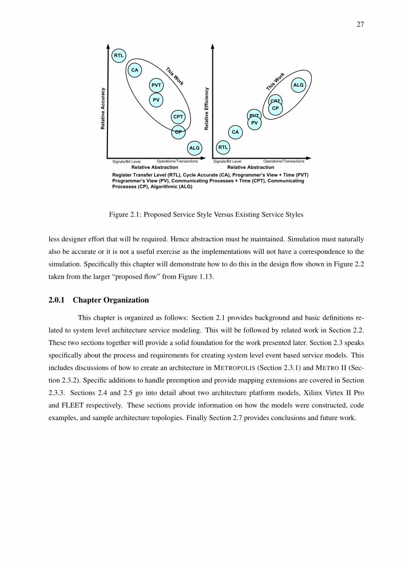
27
Relative Accuracy
Relative Abstraction
RTL
Signals/Bit Level Operations/Transactions
Relative Efficiency
Relative Abstraction
RTLALG
Signals/Bit Level Operations/Transactions
CA
PVT
PV
CPT
CP
Register Transfer Level (RTL), Cycle Accurate (CA), Programmer’s View + Time (PVT)
Programmer’s View (PV), Communicating Processes + Time (CPT), Communicating
Processes (CP), Algorithmic (ALG)
CA
PVT
PV
CPT
CP
ALG
Figure 2.1: Proposed Service Style Versus Existing Service Styles
less designer effort that will be required. Hence abstraction must be maintained. Simulation must naturally
also be accurate or it is not a useful exercise as the implementations will not have a correspondence to the
simulation. Specifically this chapter will demonstrate how to do this in the design flow shown in Figure 2.2
taken from the larger “proposed flow” from Figure 1.13.
2.0.1 Chapter Organization
This chapter is organized as follows: Section 2.1 provides background and basic definitions re-
lated to system level architecture service modeling. This will be followed by related work in Section 2.2.
These two sections together will provide a solid foundation for the work presented later. Section 2.3 speaks
specifically about the process and requirements for creating system level event based service models. This
includes discussions of how to create an architecture in METROPOLIS (Section 2.3.1) and METRO II (Sec-
tion 2.3.2). Specific additions to handle preemption and provide mapping extensions are covered in Section
2.3.3. Sections 2.4 and 2.5 go into detail about two architecture platform models, Xilinx Virtex II Pro
and FLEET respectively. These sections provide information on how the models were constructed, code
examples, and sample architecture topologies. Finally Section 2.7 provides conclusions and future work.
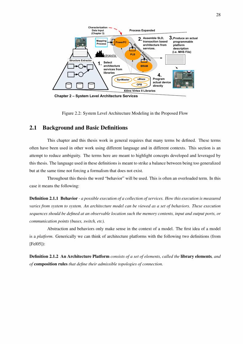
28
Chapter 2 – System Level Architecture Services
Select
architecture
services from
libraries
Assemble SLD,
transaction based
architecture from
services.
Produce an actual
programmable
platform
description
(i.e. MHS File)
Program
actual device
directly
Process Expanded
Structure Extractor
BRAM
PowerPC
PLB
Mapping
Process
Xilinx Virtex II Libraries
OPB
SynMaster uBlaze
Structure E
xtraction
Characterization
Data Input
(Chapter 3)
Figure 2.2: System Level Architecture Modeling in the Proposed Flow
2.1 Background and Basic Definitions
This chapter and this thesis work in general requires that many terms be defined. These terms
often have been used in other work using different language and in different contexts. This section is an
attempt to reduce ambiguity. The terms here are meant to highlight concepts developed and leveraged by
this thesis. The language used in these definitions is meant to strike a balance between being too generalized
but at the same time not forcing a formalism that does not exist.
Throughout this thesis the word “behavior” will be used. This is often an overloaded term. In this
case it means the following:
Definition 2.1.1 Behavior - a possible execution of a collection of services. How this execution is measured
varies from system to system. An architecture model can be viewed as a set of behaviors. These execution
sequences should be defined at an observable location such the memory contents, input and output ports, or
communication points (buses, switch, etc).
Abstraction and behaviors only make sense in the context of a model. The first idea of a model
is a platform. Generically we can think of architecture platforms with the following two definitions (from
[Fel05]):
Definition 2.1.2 An Architecture Platform consists of a set of elements, called the library elements, and
of composition rules that define their admissible topologies of connection.
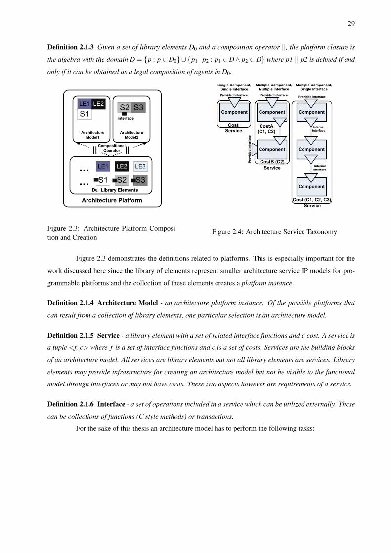
29
Definition 2.1.3 Given a set of library elements D0 and a composition operator ||, the platform closure is
the algebra with the domain D = {p : p ∈ D0}∪{p1||p2 : p1 ∈ D∧ p2 ∈ D} where p1 || p2 is defined if and
only if it can be obtained as a legal composition of agents in D0.
Library Elements
Architecture
Model1
Architecture Platform
Architecture
Model2
Interface
D0,
Compositional
Operator
Figure 2.3: Architecture Platform Composi-tion and Creation
Component
Component
Component Component
Component
Component
Single Component,
Single Interface
Multiple Component,
Multiple Interface
Multiple Component,
Single Interface
Service
Provided Interface Provided Interface
Provided Interface
Service
Cost CostA
(C1, C2)
CostB (C2)
Provided Interface
Cost (C1, C2, C3)
Service
Internal
Interface
Internal
Interface
Figure 2.4: Architecture Service Taxonomy
Figure 2.3 demonstrates the definitions related to platforms. This is especially important for the
work discussed here since the library of elements represent smaller architecture service IP models for pro-
grammable platforms and the collection of these elements creates a platform instance.
Definition 2.1.4 Architecture Model - an architecture platform instance. Of the possible platforms that
can result from a collection of library elements, one particular selection is an architecture model.
Definition 2.1.5 Service - a library element with a set of related interface functions and a cost. A service is
a tuple <f, c> where f is a set of interface functions and c is a set of costs. Services are the building blocks
of an architecture model. All services are library elements but not all library elements are services. Library
elements may provide infrastructure for creating an architecture model but not be visible to the functional
model through interfaces or may not have costs. These two aspects however are requirements of a service.
Definition 2.1.6 Interface - a set of operations included in a service which can be utilized externally. These
can be collections of functions (C style methods) or transactions.
For the sake of this thesis an architecture model has to perform the following tasks:
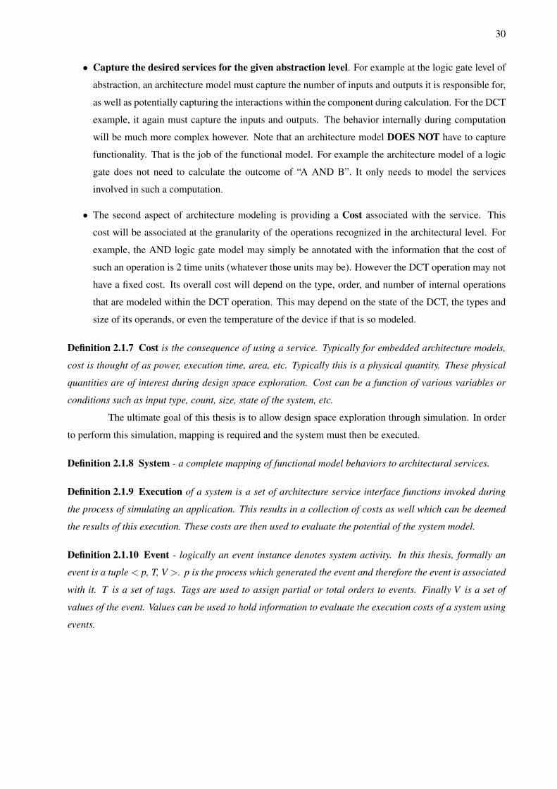
30
• Capture the desired services for the given abstraction level. For example at the logic gate level of
abstraction, an architecture model must capture the number of inputs and outputs it is responsible for,
as well as potentially capturing the interactions within the component during calculation. For the DCT
example, it again must capture the inputs and outputs. The behavior internally during computation
will be much more complex however. Note that an architecture model DOES NOT have to capture
functionality. That is the job of the functional model. For example the architecture model of a logic
gate does not need to calculate the outcome of “A AND B”. It only needs to model the services
involved in such a computation.
• The second aspect of architecture modeling is providing a Cost associated with the service. This
cost will be associated at the granularity of the operations recognized in the architectural level. For
example, the AND logic gate model may simply be annotated with the information that the cost of
such an operation is 2 time units (whatever those units may be). However the DCT operation may not
have a fixed cost. Its overall cost will depend on the type, order, and number of internal operations
that are modeled within the DCT operation. This may depend on the state of the DCT, the types and
size of its operands, or even the temperature of the device if that is so modeled.
Definition 2.1.7 Cost is the consequence of using a service. Typically for embedded architecture models,
cost is thought of as power, execution time, area, etc. Typically this is a physical quantity. These physical
quantities are of interest during design space exploration. Cost can be a function of various variables or
conditions such as input type, count, size, state of the system, etc.
The ultimate goal of this thesis is to allow design space exploration through simulation. In order
to perform this simulation, mapping is required and the system must then be executed.
Definition 2.1.8 System - a complete mapping of functional model behaviors to architectural services.
Definition 2.1.9 Execution of a system is a set of architecture service interface functions invoked during
the process of simulating an application. This results in a collection of costs as well which can be deemed
the results of this execution. These costs are then used to evaluate the potential of the system model.
Definition 2.1.10 Event - logically an event instance denotes system activity. In this thesis, formally an
event is a tuple < p, T, V >. p is the process which generated the event and therefore the event is associated
with it. T is a set of tags. Tags are used to assign partial or total orders to events. Finally V is a set of
values of the event. Values can be used to hold information to evaluate the execution costs of a system using
events.
31
Definition 2.1.11 Transaction - a collection of service interface calls. Transactions can also be one service
call which generates other service activity without explicitly calling their interfaces. This grouping is done
to add abstraction and redirection into designs.
Definition 2.1.12 Atomic Transaction a transaction which only explicitly calls a service interface. This
service must complete (the events generated are annotated and terminate) before another service can begin.
Definition 2.1.13 Annotation is the assignment of a value to an event. These annotations will typically
be considered together at the conclusion of architecture execution in order to determine various metrics by
which to evaluate the application running on a particular architecture.
2.2 Related Work
When discussing related work in system level architecture service modeling there are many com-
parisons and there are many approaches that can be examined. These approaches can be divided into those
which are industrially developed and those which are academic based. Additionally, these approaches can
be placed in a platform-based design flow. This placement allows them to be divided into those which just
allow a platform description (P) or a platform description plus mapping capabilities (PM). This is exactly
how the taxonomy in [Dou06c] is constructed. This section will present a brief overview of that work along
with providing other insights into how this thesis fits into the existing system level design landscape.
In the language development domain there is primarily SystemC [Ope07]. This is by far the most
recognized system level architecture development language. SystemC is a set of libraries built on top of
C++ which allows for concurrent module simulation, event synchronization, and a variety of elements which
facilitate architecture descriptions. The core is an event driven simulator using events and processes. The
extensions include providing for concurrent behavior, a notion of time sequenced operations, data types for
describing hardware, structure hierarchy, and simulation support. Accellera’s SystemVerilog [Acc07] is an
extension of verilog which adds system level features. For example it can co-simulate with C/C++/SystemC
code, includes support for assertion based verification (ABV), and provides extended data types and eases
restrictions on type usage. Unified Modeling Language (UML) [Uni07] is another well known language
which is in this space. UML allows for the abstract specification of a system using a graphical set of
diagrams. It is used to illustrate the system topology and the relationship between components.
In the industrial domain, tools which focus on platform descriptions (P) include such tools as
Prosilog’s Nepsys [Pro07]. This tool relies on IP libraries based on SystemC. It works at the component,
transaction level. Beach Solution’s EASI-Studio [Bea07] focuses on interconnection issues at the component
32
level and provides solutions to package IP in a repeatable, reliable manner. The suite provides a collection
of tools which help to manage the design. These tools include data import features, graphical interface
capture, and IP watermarking. Of particular interest are its Specification Rule Checks (SRC) which ensure
adherence to naming conventions, name uniqueness, address space uniqueness, and that parameter values
are resolvable. Sonics’ Sonics Studio [Son07] works at the implementation level by using bus functional
models (BFM). This tool includes a graphical, drag and drop environment for configuring SoC designs. This
environment also provides monitor functions and simulation support for IP blocks.
Industrial domain tools for creating platform descriptions with mapping capabilities (PM) include
VaST Systems Technology’s Comet/Meteor [VaS07]. The Comet tool focuses on high performance proces-
sor and architecture models at the system level. This tool uses virtual processors, buses, and peripheral
devices. Meteor is an embedded software development environment. It also accepts virtual system proto-
types for cycle accurate simulation and parameter driven configuration. Finally Summit’s System Architect
[Sum07] looks at multi-core SoCs and large scale systems. This is a SystemC component based system.
Summit has been recently acquired by Mentor Graphics.
Finally, industrial tools with functional, platform, and mapping capabilities (FPM) include MLDe-
sign’s MLDesigner [MLD07]. This tool allows for discrete event, dynamic dataflow, and synchronous
dataflow model of computation to be described. It is intended to be used for a “top-down” design flow start-
ing from initial specification to final implementation. It includes an integrated development environment
(IDE) to integrate all aspects in one package. Mirabilis Design’s Visual Sim [Mir07] product family adds
continuous time and finite state machine (FSM) models of computation natively to this list of supported
MoCs (they are also available in the experimental library of MLDesigner but as of the time of the work, they
are in the beta stage). The design process in Visual Sim begins by constructing a model of the system using
the parameterizable library provided. This model can be augmented as well with C, C++, Java, SystemC,
Verilog, or VHDL blocks. The library blocks operate semantically using a wide variety of models of compu-
tation as listed. The design is then partitioning into software, middleware, or hardware. Finally the design is
optimized by running simulations and adjusting parameters of the library elements. The last industrial FPM
tool is Cofluent’s Systems Studio [CoF07]. It provides transaction level SystemC models which perform
design space exploration in the Y-chart modeling methodology. The functional description is a set of com-
municating processes executing concurrently. The platform model is a set of communicating processes and
shared memories linked by shared communication nodes. The platform model has performance attributes
associated with it as well. This approach is very similar to METROPOLIS but does not support as wide a
variety of models of computation or as rich a constraint verification infrastructure.
The academic domain has many offerings as well. An academic tool which captures the function-

33
ality of a design (F) is ForSyDe [Ing04]. This tool is a product of the Royal Institute of Technology, Sweden.
It performs modeling, simulation, and design of concurrent, real-time, embedded systems. It has support for
a wide variety of synchronous MoCs. It uses transformation rules to proceed from a functional specification
to collections of process networks.
A tool which allows platform descriptions as well as mapping (PM) is Carnegie Mellon’s MESH
[And03]. MESH stands for Modeling Environment for Software and Hardware. This approach examines
heterogeneous system design at the component level through C input. MESH is an event based approach
in which its threads are ordered sets of N events. MESH is interested as well in the development of bench-
marks, called scenarios, which evaluate collections of heterogeneous programs. Stanford’s Rapide [Dav95]
is an Executable Architecture Definition Languages (EADL). It utilizes an event based execution model for
distributed, time sensitive systems. Rapide is a PM approach as well.
Tools which add the ability to specify functional descriptions as well (FPM) include Seoul Na-
tional University’s PEACE [Soo06]. This is codesign environment which is Ptolemy based [Jos02]. It touts
an open-source framework, a reconfigurable framework (design steps are decoupled so that users can intro-
duce their own steps), a separate Java based GUI (named Hae) from the kernel, an objected-oriented C++
kernel, support for multilingual system design (dataflow graphs for functional representations and FSMs for
control), and automatic hardware/software synthesis as its strengths. UC Berkeley’s MESCAL [And02] is an
approach for the programming of application specific programmable platforms. It has extended Ptolemy II
[Joh01] and has focused recently on network processors. Vanderbilt’s GME/GREAT/DESERT [Ako01] are
a set of tools for pruning the design space. Aspects of it are UML and XML based. It is focused on domain
specific modeling and program synthesis. Finally, Spade from Delft University of Technology [Pau01a] is
a kahn process network (KPN) based workbench. It also employs a Y-chart based approach to design with
functionality and architecture separated. In this case they are termed workload and resources respectively.
It employs trace driven simulation where time can be accounted for and performance data collected.
All of these academic and industrial tools work at the system level in terms of the level of abstrac-
tion employed.
As mentioned, each of these approaches are placed in a taxonomy in [Dou06c]. Without going
into all the details contained in that work, one can say that the following issues are investigated: model of
computation supported, support for quantity annotation, mapping support, specific device support (ASIC,
FPGA, etc), level of abstraction supported, and underlying semantics. The reader would be well served to
look at that work as it covers 90+ tools.
Table 2.1 has a small sample of the comparisons that can be made between METROPOLIS and
other academic (top half) and industrial (bottom half) approaches. The issues outlined, Event Based, Map-
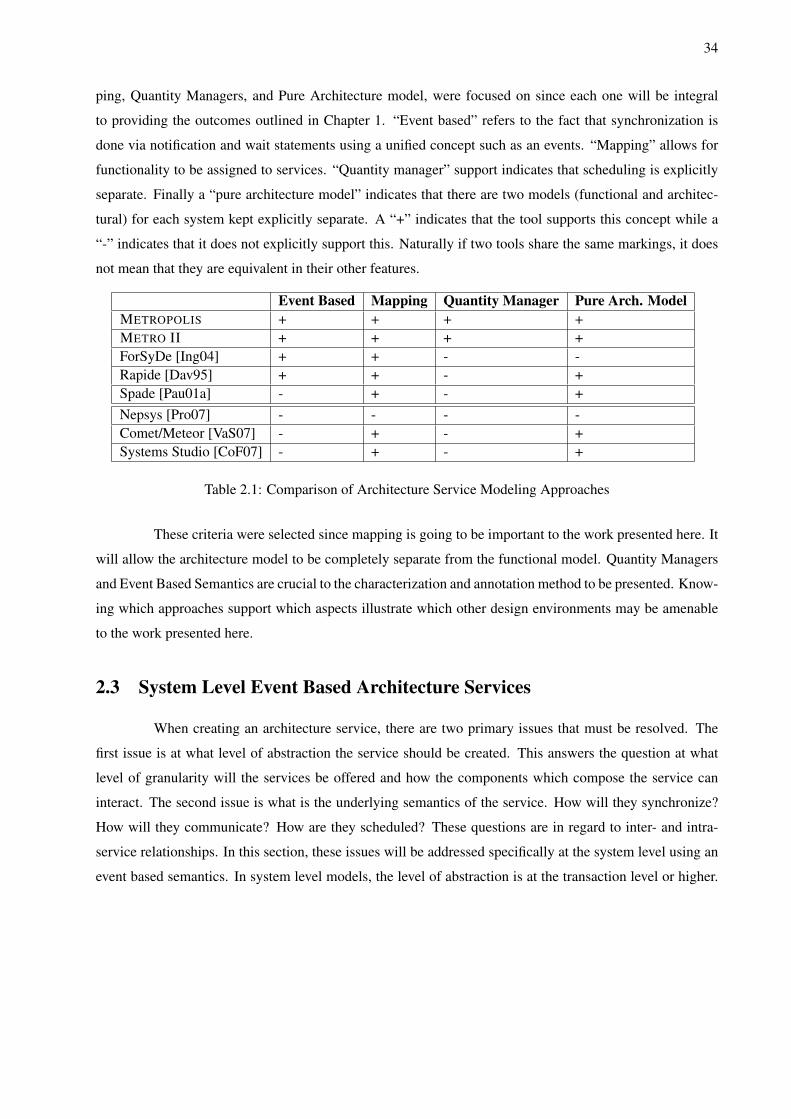
34
ping, Quantity Managers, and Pure Architecture model, were focused on since each one will be integral
to providing the outcomes outlined in Chapter 1. “Event based” refers to the fact that synchronization is
done via notification and wait statements using a unified concept such as an events. “Mapping” allows for
functionality to be assigned to services. “Quantity manager” support indicates that scheduling is explicitly
separate. Finally a “pure architecture model” indicates that there are two models (functional and architec-
tural) for each system kept explicitly separate. A “+” indicates that the tool supports this concept while a
“-” indicates that it does not explicitly support this. Naturally if two tools share the same markings, it does
not mean that they are equivalent in their other features.
Event Based Mapping Quantity Manager Pure Arch. ModelMETROPOLIS + + + +METRO II + + + +ForSyDe [Ing04] + + - -Rapide [Dav95] + + - +Spade [Pau01a] - + - +Nepsys [Pro07] - - - -Comet/Meteor [VaS07] - + - +Systems Studio [CoF07] - + - +
Table 2.1: Comparison of Architecture Service Modeling Approaches
These criteria were selected since mapping is going to be important to the work presented here. It
will allow the architecture model to be completely separate from the functional model. Quantity Managers
and Event Based Semantics are crucial to the characterization and annotation method to be presented. Know-
ing which approaches support which aspects illustrate which other design environments may be amenable
to the work presented here.
2.3 System Level Event Based Architecture Services
When creating an architecture service, there are two primary issues that must be resolved. The
first issue is at what level of abstraction the service should be created. This answers the question at what
level of granularity will the services be offered and how the components which compose the service can
interact. The second issue is what is the underlying semantics of the service. How will they synchronize?
How will they communicate? How are they scheduled? These questions are in regard to inter- and intra-
service relationships. In this section, these issues will be addressed specifically at the system level using an
event based semantics. In system level models, the level of abstraction is at the transaction level or higher.

35
This answers the first question. The semantics that will be discussed here are those which use events during
simulation for a variety of issues including synchronization, annotation, and communication. The answers
the second question.
System level event based services are of particular interest for two reasons. First the level of ab-
straction directly attacks the level of complexity currently seen in designs today. Additionally, it allows rapid
design space exploration. Event based frameworks are useful since a wide variety of models of computation
can easily be framed using events. Events also have the ability to carry the service cost along with them in
the form of an event value. This makes such frameworks very flexible.
An event is the fundamental concept in the framework of solutions described. In METROPOLIS
for example, an event represents a transition in the action automata of an object under simulation. An event
is owned by the object that exports it and during simulation, generated events are termed as event instances.
Events can be annotated with any number of quantities (i.e. costs). In addition, events can partially expose
the state around them and constraints can then reference or influence this state.
A system level service is a collection of components (library elements). Each of the components
have interfaces which expose their capabilities to other components. A service requires that at least one of
the interfaces is exposed to the functional model or to other services. These interfaces are called provided
interfaces. Interfaces between components making up the service alone are called internal interfaces. A
service can be composed of a single or multiple components. If more than one component has a provided
interface, then it is considered having multiple interfaces. Multiple interfaces allow for a service to have
more than one cost model.
A service ultimately then corresponds to a set of event sequences generated by collections of
components with various sets of interfaces with various costs. This execution therefore represents one
possible behavior of a system. Here is the taxonomy of service types at the system level (as shown in Figure
2.4):
• Single Component, Single Interface (SCSI) - a service composed of a single component. The pro-
vided interface is the only interface provided to the functional description or other services. There is
only one cost model provided with this service which is accessed through the single interface.
• Multiple Component, Single Interface (MCSI) - a service composed of multiple components. Only
one of the components has a provided interface. The presence of multiple components allows for a
more complicated cost model, hierarchical composition of services, and hierarchical interfaces. Only
one cost model is provided to the functional description.

36
• Multiple Component, Multiple Interface (MCMI) - a service composed of multiple components
with multiple provided interfaces. This configuration allows for multiple cost models along with the
advantages of a MCSI configuration.
Notice that single component, multiple interface (SCMI) services are not present because this
scenario does not make sense given the fact that there are no multiple interfaces to allow for various inter-
service component interactions (and hence generate different cost models). Note that SCSI services can
return different cost values based on the parameters provided to the interface. They are just restricted to one
cost model.
Services can also be active or passive. An active service is a service which can generate interface
calls. This can be thought of as a component which has an executing thread. A passive service is one which
responds to interface calls. Naturally this response could in turn cause it to trigger an interface call itself.
Architecture topologies can be formed as well using collections of these types of services. Ulti-
mately it is these topologies which form the architecture model. For example there are two primary styles.
The first is a branching structure. This allows for services that use all types of service categorizations. This
is illustrated in Figure 2.5 of the left. A branching structure is one in which services are connected in such
a way that a service may interact with any number of other services. For example a bus service can interact
with two or more computation services and a memory service. A ring structure on the other hand only allows
for single interface services (SCSI, MCSI). This is illustrated in Figure 2.5 on the right. A ring structure
can be useful for certain networking topologies. Also this structure often simplifies the scheduling problem
as well as an analysis of its execution. Of course it is possible to have mixed topologies in which various
aspects can be classified as either branching or ring.
Definition 2.3.1 System Level Architecture Modeling - a collection of services at the transaction level or
higher of abstraction. These services can be classified as SCSI, MCSI, or MCMI. Additionally the topology
of the system can be defined as branching, ring, or a hybrid of the two.
The next sections (2.3.1 and 2.3.2) will detail two system level event based environments, METROPO-
LIS and METRO II. These sections will detail the components in the framework and the ways in which
architecture models are created.
2.3.1 METROPOLIS Architecture Construction
The work presented here in this thesis is built heavily on METROPOLIS. This is a system level
design language with an event based semantics. This framework was described at a high level in Section 1.2.
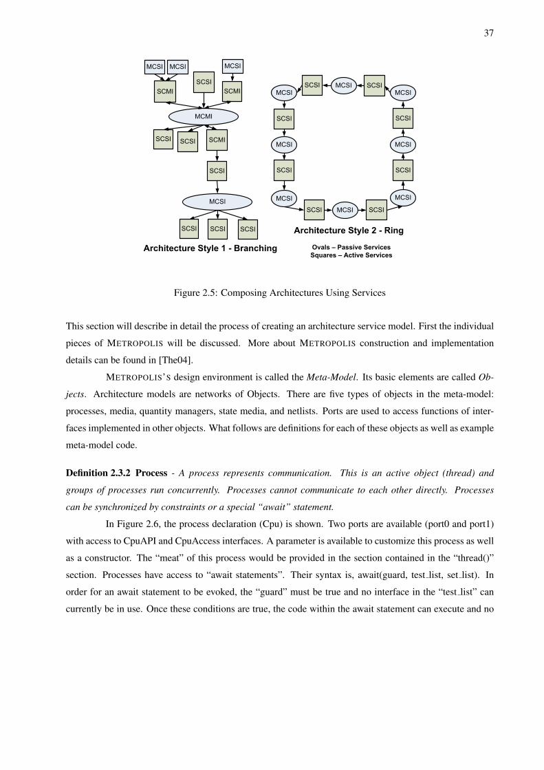
37
Ovals – Passive Services
Squares – Active Services
Figure 2.5: Composing Architectures Using Services
This section will describe in detail the process of creating an architecture service model. First the individual
pieces of METROPOLIS will be discussed. More about METROPOLIS construction and implementation
details can be found in [The04].
METROPOLIS’S design environment is called the Meta-Model. Its basic elements are called Ob-
jects. Architecture models are networks of Objects. There are five types of objects in the meta-model:
processes, media, quantity managers, state media, and netlists. Ports are used to access functions of inter-
faces implemented in other objects. What follows are definitions for each of these objects as well as example
meta-model code.
Definition 2.3.2 Process - A process represents communication. This is an active object (thread) and
groups of processes run concurrently. Processes cannot communicate to each other directly. Processes
can be synchronized by constraints or a special “await” statement.
In Figure 2.6, the process declaration (Cpu) is shown. Two ports are available (port0 and port1)
with access to CpuAPI and CpuAccess interfaces. A parameter is available to customize this process as well
as a constructor. The “meat” of this process would be provided in the section contained in the “thread()”
section. Processes have access to “await statements”. Their syntax is, await(guard, test list, set list). In
order for an await statement to be evoked, the “guard” must be true and no interface in the “test list” can
currently be in use. Once these conditions are true, the code within the await statement can execute and no
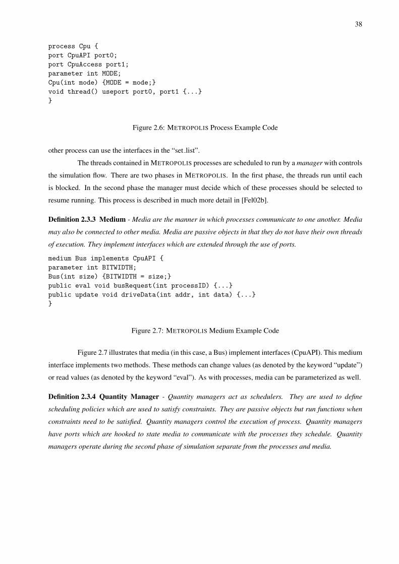
38
process Cpu {port CpuAPI port0;port CpuAccess port1;parameter int MODE;Cpu(int mode) {MODE = mode;}void thread() useport port0, port1 {...}}
Figure 2.6: METROPOLIS Process Example Code
other process can use the interfaces in the “set list”.
The threads contained in METROPOLIS processes are scheduled to run by a manager with controls
the simulation flow. There are two phases in METROPOLIS. In the first phase, the threads run until each
is blocked. In the second phase the manager must decide which of these processes should be selected to
resume running. This process is described in much more detail in [Fel02b].
Definition 2.3.3 Medium - Media are the manner in which processes communicate to one another. Media
may also be connected to other media. Media are passive objects in that they do not have their own threads
of execution. They implement interfaces which are extended through the use of ports.
medium Bus implements CpuAPI {parameter int BITWIDTH;Bus(int size) {BITWIDTH = size;}public eval void busRequest(int processID) {...}public update void driveData(int addr, int data) {...}}
Figure 2.7: METROPOLIS Medium Example Code
Figure 2.7 illustrates that media (in this case, a Bus) implement interfaces (CpuAPI). This medium
interface implements two methods. These methods can change values (as denoted by the keyword “update”)
or read values (as denoted by the keyword “eval”). As with processes, media can be parameterized as well.
Definition 2.3.4 Quantity Manager - Quantity managers act as schedulers. They are used to define
scheduling policies which are used to satisfy constraints. They are passive objects but run functions when
constraints need to be satisfied. Quantity managers control the execution of process. Quantity managers
have ports which are hooked to state media to communicate with the processes they schedule. Quantity
managers operate during the second phase of simulation separate from the processes and media.
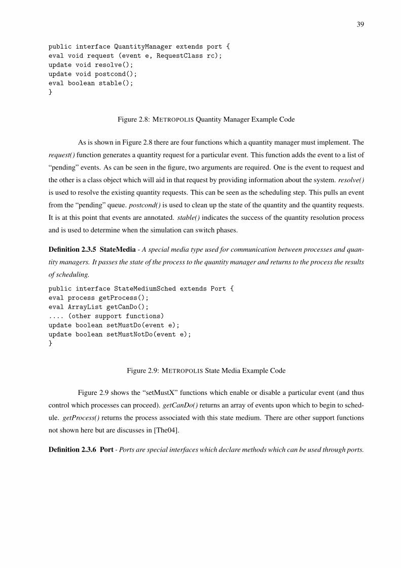
39
public interface QuantityManager extends port {eval void request (event e, RequestClass rc);update void resolve();update void postcond();eval boolean stable();}
Figure 2.8: METROPOLIS Quantity Manager Example Code
As is shown in Figure 2.8 there are four functions which a quantity manager must implement. The
request() function generates a quantity request for a particular event. This function adds the event to a list of
“pending” events. As can be seen in the figure, two arguments are required. One is the event to request and
the other is a class object which will aid in that request by providing information about the system. resolve()
is used to resolve the existing quantity requests. This can be seen as the scheduling step. This pulls an event
from the “pending” queue. postcond() is used to clean up the state of the quantity and the quantity requests.
It is at this point that events are annotated. stable() indicates the success of the quantity resolution process
and is used to determine when the simulation can switch phases.
Definition 2.3.5 StateMedia - A special media type used for communication between processes and quan-
tity managers. It passes the state of the process to the quantity manager and returns to the process the results
of scheduling.
public interface StateMediumSched extends Port {eval process getProcess();eval ArrayList getCanDo();.... (other support functions)update boolean setMustDo(event e);update boolean setMustNotDo(event e);}
Figure 2.9: METROPOLIS State Media Example Code
Figure 2.9 shows the “setMustX” functions which enable or disable a particular event (and thus
control which processes can proceed). getCanDo() returns an array of events upon which to begin to sched-
ule. getProcess() returns the process associated with this state medium. There are other support functions
not shown here but are discusses in [The04].
Definition 2.3.6 Port - Ports are special interfaces which declare methods which can be used through ports.
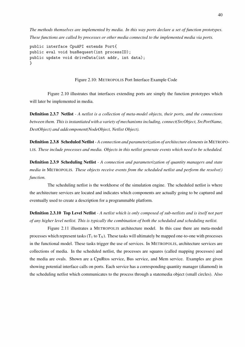
40
The methods themselves are implemented by media. In this way ports declare a set of function prototypes.
These functions are called by processes or other media connected to the implemented media via ports.
public interface CpuAPI extends Port{public eval void busRequest(int processID);public update void driveData(int addr, int data);}
Figure 2.10: METROPOLIS Port Interface Example Code
Figure 2.10 illustrates that interfaces extending ports are simply the function prototypes which
will later be implemented in media.
Definition 2.3.7 Netlist - A netlist is a collection of meta-model objects, their ports, and the connections
between them. This is instantiated with a variety of mechanisms including, connect(SrcObject, SrcPortName,
DestObject) and addcomponent(NodeObject, Netlist Object).
Definition 2.3.8 Scheduled Netlist - A connection and parameterization of architecture elements in METROPO-
LIS. These include processes and media. Objects in this netlist generate events which need to be scheduled.
Definition 2.3.9 Scheduling Netlist - A connection and parameterization of quantity managers and state
media in METROPOLIS. These objects receive events from the scheduled netlist and perform the resolve()
function.
The scheduling netlist is the workhorse of the simulation engine. The scheduled netlist is where
the architecture services are located and indicates which components are actually going to be captured and
eventually used to create a description for a programmable platform.
Definition 2.3.10 Top Level Netlist - A netlist which is only composed of sub-netlists and is itself not part
of any higher level netlist. This is typically the combination of both the scheduled and scheduling netlist.
Figure 2.11 illustrates a METROPOLIS architecture model. In this case there are meta-model
processes which represent tasks (T1 to TN). These tasks will ultimately be mapped one-to-one with processes
in the functional model. These tasks trigger the use of services. In METROPOLIS, architecture services are
collections of media. In the scheduled netlist, the processes are squares (called mapping processes) and
the media are ovals. Shown are a CpuRtos service, Bus service, and Mem service. Examples are given
showing potential interface calls on ports. Each service has a corresponding quantity manager (diamond) in
the scheduling netlist which communicates to the process through a statemedia object (small circles). Also
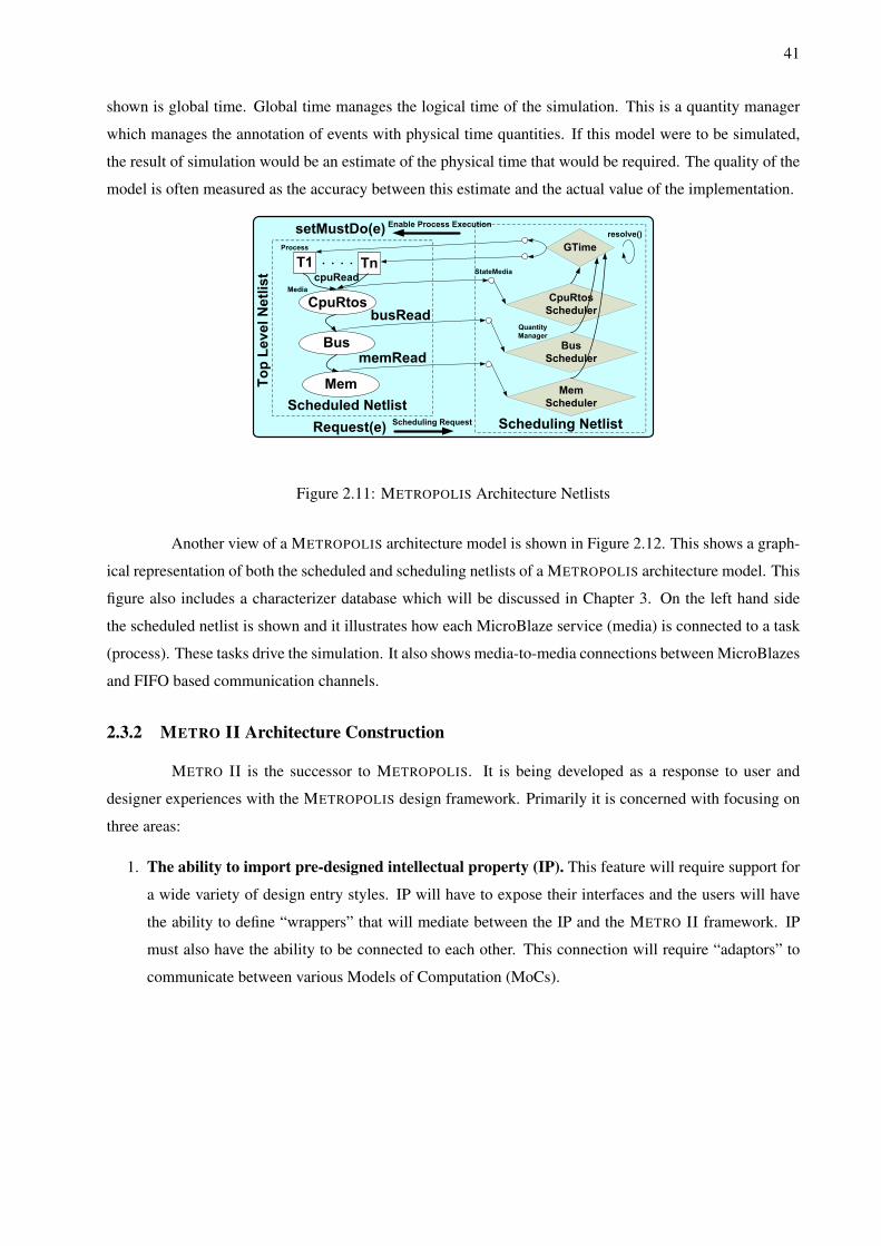
41
shown is global time. Global time manages the logical time of the simulation. This is a quantity manager
which manages the annotation of events with physical time quantities. If this model were to be simulated,
the result of simulation would be an estimate of the physical time that would be required. The quality of the
model is often measured as the accuracy between this estimate and the actual value of the implementation.
cpuRead
CpuRtos
Scheduler
Bus
Scheduler
Mem
Scheduler
GTime
resolve()
Media
Process
StateMedia
Quantity
Manager
Scheduling Request
Enable Process Execution
Figure 2.11: METROPOLIS Architecture Netlists
Another view of a METROPOLIS architecture model is shown in Figure 2.12. This shows a graph-
ical representation of both the scheduled and scheduling netlists of a METROPOLIS architecture model. This
figure also includes a characterizer database which will be discussed in Chapter 3. On the left hand side
the scheduled netlist is shown and it illustrates how each MicroBlaze service (media) is connected to a task
(process). These tasks drive the simulation. It also shows media-to-media connections between MicroBlazes
and FIFO based communication channels.
2.3.2 METRO II Architecture Construction
METRO II is the successor to METROPOLIS. It is being developed as a response to user and
designer experiences with the METROPOLIS design framework. Primarily it is concerned with focusing on
three areas:
1. The ability to import pre-designed intellectual property (IP). This feature will require support for
a wide variety of design entry styles. IP will have to expose their interfaces and the users will have
the ability to define “wrappers” that will mediate between the IP and the METRO II framework. IP
must also have the ability to be connected to each other. This connection will require “adaptors” to
communicate between various Models of Computation (MoCs).
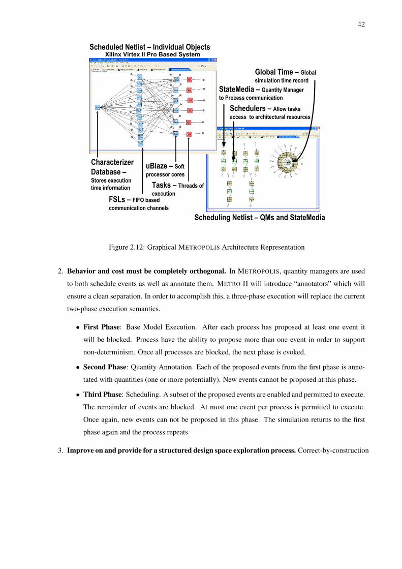
42
Tasks – Threads of execution
uBlaze – Soft processor cores
FSLs – FIFO based communication channels
Characterizer
Database –Stores execution
time information
Global Time – Global simulation time record
StateMedia – Quantity Manager to Process communication
Scheduled Netlist – Individual Objects
Scheduling Netlist – QMs and StateMedia
Xilinx Virtex II Pro Based System
Schedulers – Allow tasks access to architectural resources
Figure 2.12: Graphical METROPOLIS Architecture Representation
2. Behavior and cost must be completely orthogonal. In METROPOLIS, quantity managers are used
to both schedule events as well as annotate them. METRO II will introduce “annotators” which will
ensure a clean separation. In order to accomplish this, a three-phase execution will replace the current
two-phase execution semantics.
• First Phase: Base Model Execution. After each process has proposed at least one event it
will be blocked. Process have the ability to propose more than one event in order to support
non-determinism. Once all processes are blocked, the next phase is evoked.
• Second Phase: Quantity Annotation. Each of the proposed events from the first phase is anno-
tated with quantities (one or more potentially). New events cannot be proposed at this phase.
• Third Phase: Scheduling. A subset of the proposed events are enabled and permitted to execute.
The remainder of events are blocked. At most one event per process is permitted to execute.
Once again, new events can not be proposed in this phase. The simulation returns to the first
phase again and the process repeats.
3. Improve on and provide for a structured design space exploration process. Correct-by-construction
43
techniques and streamlining the mapping process will be keys to this improvement.
The building blocks of METRO II are: components, ports, connections, constraints (and asser-
tions), adaptors, mappers, annotators, and schedulers. Each of these is described in detail in [Abh07]. This
thesis will not focus on describing these in more detail individually but will rather propose how to use them
to build services and hence an architecture model.
Figure 2.13 provides sample constructions of SCSI, MCSI, MCMI services built from METRO
II components. Each of the services are either composed of one or multiple METRO II components as
denoted by their classification. In addition, all components which constitute a service are encompassed by a
“wrapper”. This wrapper becomes the boundary of the service upon which the provided interfaces and the
cost of the service are defined. This wrapper will provide a consistent global interface to all other services
to facilitate their connection. These connections will create the architecture model itself. Additionally each
service is provided with a scheduler and annotator. The scheduler will be used in the third phase of the
service’s execution and the annotator provides the cost model for the service in the second phase. Service
“provided interfaces” of the wrapper are connected to METRO II “provided ports” of select components. One
set of METRO II “required ports” is visible at the wrapper interface to allow the service to take advantage
of other services if need be.
Each service classification (SCSI, MCSI, MCMI) differs in how many METRO II “view ports”
are provided to the wrapper. View ports can be used to observe the operation of the service. These ports
will be useful in creating structures to verify properties of the service (and hence architecture). In the case
of SCSI and MCSI, there will only be one view port provided. This port corresponds with the component
which connects its provided port to the wrapper’s provided interface. In the case of MCMI, each component
with provided ports serving as provided interfaces will have its view port present at the wrapper level.
Additionally in MCSI and MCMI, “rendezvous ports” are required to synchronize the components. In
MCSI, rendezvous ports between all components with provided/required port relationships are connected.
In MCMI, rendezvous ports are connected between components with provided/required port relationships
provided that at least one of the two components does not contribute to the provided interface.
Both branching and ring architecture styles can be created using these service types. Whereas
METROPOLIS required that active services have processes and passive services have media, METRO II does
not have this distinction. All services are only composed of components. This potentially leads to more
flexibility in specification or dual operating mode services (a switch that indicates if the service is passive or
active). METROPOLIS required that mapping tasks be provided with the architecture model as active objects
by which the functional model can be mapped to. This is not needed in METRO II. A provided interface
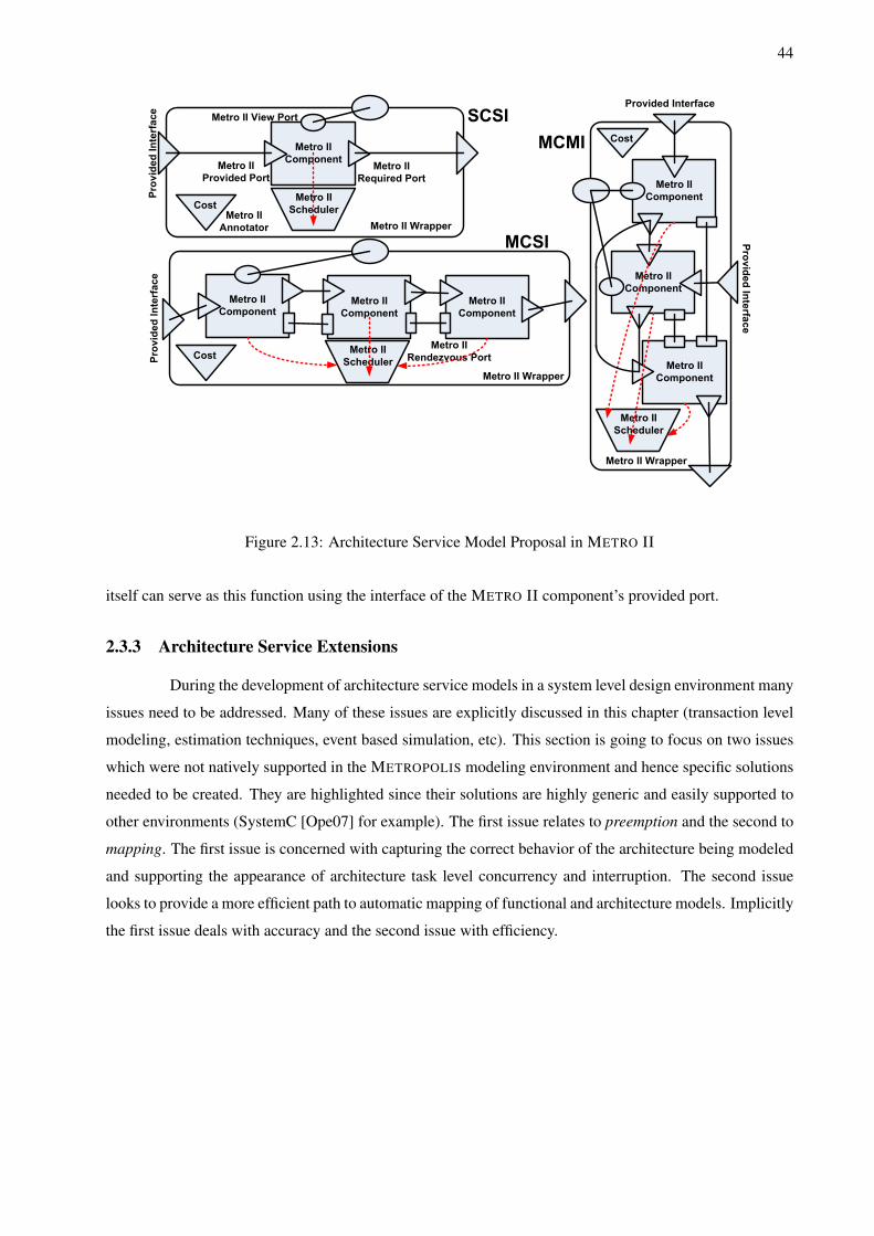
44
Metro II
Component
Metro II
Component
Metro II
ComponentMetro II
Provided Port
Metro II
Required Port
Metro II
Scheduler
Metro II View Port
Metro II
Component
Metro II
Scheduler
Metro II Wrapper
Metro II Wrapper
Metro II
Rendezvous PortProvided Interface
Provided Interface
Metro II
Component
Metro II
Component
Metro II
Component
Metro II
Scheduler
Metro II Wrapper
Provided Interface
Metro II
Annotator
Cost
Cost
Provided Interface
Cost
Figure 2.13: Architecture Service Model Proposal in METRO II
itself can serve as this function using the interface of the METRO II component’s provided port.
2.3.3 Architecture Service Extensions
During the development of architecture service models in a system level design environment many
issues need to be addressed. Many of these issues are explicitly discussed in this chapter (transaction level
modeling, estimation techniques, event based simulation, etc). This section is going to focus on two issues
which were not natively supported in the METROPOLIS modeling environment and hence specific solutions
needed to be created. They are highlighted since their solutions are highly generic and easily supported to
other environments (SystemC [Ope07] for example). The first issue relates to preemption and the second to
mapping. The first issue is concerned with capturing the correct behavior of the architecture being modeled
and supporting the appearance of architecture task level concurrency and interruption. The second issue
looks to provide a more efficient path to automatic mapping of functional and architecture models. Implicitly
the first issue deals with accuracy and the second issue with efficiency.
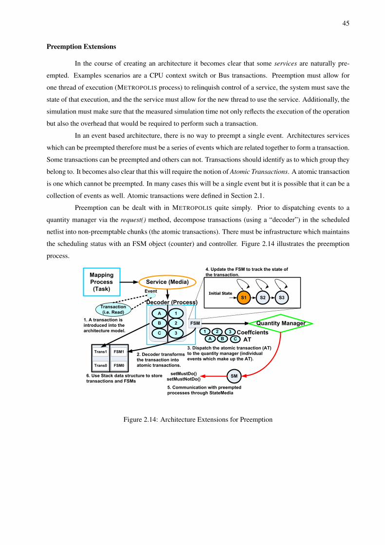
45
Preemption Extensions
In the course of creating an architecture it becomes clear that some services are naturally pre-
empted. Examples scenarios are a CPU context switch or Bus transactions. Preemption must allow for
one thread of execution (METROPOLIS process) to relinquish control of a service, the system must save the
state of that execution, and the the service must allow for the new thread to use the service. Additionally, the
simulation must make sure that the measured simulation time not only reflects the execution of the operation
but also the overhead that would be required to perform such a transaction.
In an event based architecture, there is no way to preempt a single event. Architectures services
which can be preempted therefore must be a series of events which are related together to form a transaction.
Some transactions can be preempted and others can not. Transactions should identify as to which group they
belong to. It becomes also clear that this will require the notion of Atomic Transactions. A atomic transaction
is one which cannot be preempted. In many cases this will be a single event but it is possible that it can be a
collection of events as well. Atomic transactions were defined in Section 2.1.
Preemption can be dealt with in METROPOLIS quite simply. Prior to dispatching events to a
quantity manager via the request() method, decompose transactions (using a “decoder”) in the scheduled
netlist into non-preemptable chunks (the atomic transactions). There must be infrastructure which maintains
the scheduling status with an FSM object (counter) and controller. Figure 2.14 illustrates the preemption
process.
Initial State
Transaction
(i.e. Read)
Decoder (Process)
1. A transaction is
introduced into the
architecture model.
1
3
2
2. Decoder transforms
the transaction into
atomic transactions.
3. Dispatch the atomic transaction (AT)
to the quantity manager (individual
events which make up the AT).
1 2 3
4. Update the FSM to track the state of
the transaction.
S1 S3S2
Service (Media)
Mapping
Process
(Task)
FSM
A
C
B Quantity Manager
Event
A B C
Trans1 FSM1
Trans0 FSM0
SMsetMustDo()
setMustNotDo()
5. Communication with preempted
processes through StateMedia
6. Use Stack data structure to store
transactions and FSMs
Coeffcients
AT
Figure 2.14: Architecture Extensions for Preemption
46
Figure 2.14 illustrates the preemption process. There are several stages involved in the process:
1. A transaction is introduced into the architecture model. This is done by the mapping process which is
mapped to the tasks in the functional model. This is a single event generated by a task process in the
scheduled netlist.
2. The transaction proceeds to a decoder object (process) connected to the service media. This decoder
must perform several tasks:
• Identify if the transaction is atomic or not. This is done through a table lookup or by a transaction
argument detailing its status.
• In the event that it is not atomic, decompose it into atomic transactions (A, B, C in the figure).
Each atomic transaction is typically made up of transactions from SCSI services but it does not
have to be, it just will raise the notion of atomic to contain more components. Often atomic
transactions are defined around provided interfaces of services.
• Augment the atomic events with information regarding architecture execution. This is a coeffi-
cient which will be used to ensure that each atomic event takes a fraction of the total execution
time for the entire transaction. Coefficients can be created dynamically using simple floating
point operations.
• Introduce events to represent the overhead associated with the preemption type (1, 2, 3 in the
figure). These events will also have a coefficient value. How to generate these events, how many
of them, and their cost is determined by the decoder.
• Create a finite state machine. The number of states is a one-hot encoding based on the number
of atomic transactions. Each atomic transaction now has a partial ordering assigned to it. It is a
partial ordering since atomic transactions may issue nondeterministically.
3. Dispatch (request()) the atomic transactions as normal to the quantity manager. Here they will go
through the standard resolve(), postcond(), stable() iterations.
4. Update the FSM to track the state of the transaction as a whole. When no transition can be made, the
transaction is considered complete. In the event that a new FSM has been created by a preemptive
process, you should push the existing FSM requests on a stack and pop them off as other FSM finish.
This is assuming a LIFO preemption policy.
5. Use statemedia to communicate with processes using the setMustDo() and setMustNotDo() functions.
The preempted process will be blocked whereas the preempting process will be allowed to proceed.
47
6. There is a decoder assigned to each service which supports preemption. In the event that preemption
occurs, the FSM and bundled atomic events are pushed onto a stack (LIFO object). Each decoder
(and hence services supporting preemption) has its own stack. Once the preemption is done, the stack
is popped and execution continues. Once the FSM reaches the final state, the information for that
transaction is discarded and the stack can be popped again.
This approach can be improved to some extent by a more compact FSM encoding but at the
level of abstraction required by transaction level modeling, there will rarely be more than ten states in any
transaction. In addition the time required for the overhead of a preemption is unique to each service and
must be provided by the designer.
Mapping Extensions
A unique aspect of programmable platforms is that they allow for both SW and HW implemen-
tations of a function. For example there may be a soft processor model (Xilinx MicroBlaze for example)
which can perform a SW routine for DCT. Additionally there may be a dedicated DCT block in the program-
mable logic fabric. At some point one may want to explore automated mapping of functionality to services.
A service which provides general purpose processing can handle a wide variety of functionality mappings
whereas a service for a specific HW component can only offer one type of functionality. In is not appro-
priate to map functionality to any architecture block. If this was done, services would not be available to
the functional netlist and minimally the simulation would halt, if not fail altogether. Not to mention that not
all architecture blocks can as efficiently perform operations. Not knowing the service capabilities severely
limits the ability to do intelligent mapping. Therefore there is the need to express which architecture compo-
nents can provide which services and with what affinity. Affinity refers to how well the service can provide
the desired operation. For example, an ASIC service providing an “ADD” service will have a high affinity to
provide this service if it has a lower cost (execution time perhaps) than a general purpose processor software
service “ADD”. This information is used for mapping of functionality to architecture models. Mapping can
employ greedy, task specific, or other strategies to maintain the best average affinity rating over all mapped
tasks. An example of the information provided to the mapping network is shown in Figure 2.15.
In Figure 2.15 there are two processes (tasks) connected each to their own media (service). The
service on the left is a HW Discreet Cosign Transform (DCT). The service on the right is a MicroBlaze
soft processor model (think of this a a general purpose computation service). The mapping processes are
equipped with two functions. One function can be queried to return all of the services that it has access to.
In this picture, the task on the right has access to a service which can provide execute (generically), DCT,
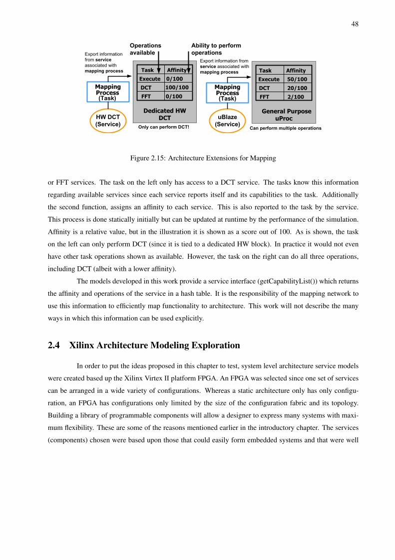
48
Mapping Process
Mapping Process
Dedicated HW DCT
General PurposeuProc
FFT
DCT
Execute
AffinityTask
0/100
100/100
0/100 2/100FFT
20/100DCT
50/100
Affinity
Execute
Task
Export information
from service
associated with
mapping process
Export information from
service associated with
mapping process
HW DCT
(Service)
uBlaze
(Service)
Operations
available
Ability to perform
operations
Only can perform DCT! Can perform multiple operations
(Task) (Task)
Figure 2.15: Architecture Extensions for Mapping
or FFT services. The task on the left only has access to a DCT service. The tasks know this information
regarding available services since each service reports itself and its capabilities to the task. Additionally
the second function, assigns an affinity to each service. This is also reported to the task by the service.
This process is done statically initially but can be updated at runtime by the performance of the simulation.
Affinity is a relative value, but in the illustration it is shown as a score out of 100. As is shown, the task
on the left can only perform DCT (since it is tied to a dedicated HW block). In practice it would not even
have other task operations shown as available. However, the task on the right can do all three operations,
including DCT (albeit with a lower affinity).
The models developed in this work provide a service interface (getCapabilityList()) which returns
the affinity and operations of the service in a hash table. It is the responsibility of the mapping network to
use this information to efficiently map functionality to architecture. This work will not describe the many
ways in which this information can be used explicitly.
2.4 Xilinx Architecture Modeling Exploration
In order to put the ideas proposed in this chapter to test, system level architecture service models
were created based up the Xilinx Virtex II platform FPGA. An FPGA was selected since one set of services
can be arranged in a wide variety of configurations. Whereas a static architecture only has only configu-
ration, an FPGA has configurations only limited by the size of the configuration fabric and its topology.
Building a library of programmable components will allow a designer to express many systems with maxi-
mum flexibility. These are some of the reasons mentioned earlier in the introductory chapter. The services
(components) chosen were based upon those that could easily form embedded systems and that were well
49
defined and characterized. To this end, the IBM CoreConnect [IBM99] based IP blocks were examined.
The architecture service models created can be categorized around the basic service type they
represent.
• Computation - PowerPC, MicroBlaze, Synthetic Master, and Synthetic Slave - (4 services total)
• Communication - Processor Local Bus (PLB), On-Chip Peripheral Bus (OPB), BRAM, Fast Simplex
Link (FSL) - (4 services total)
• Coordination - PowerPC Scheduler, MicroBlaze Scheduler, PLB Scheduler, OPB Scheduler, BRAM
Scheduler, Bridge Scheduler, FSL Scheduler, and a General Scheduler - (8 schedulers total)
• Hybrid Services - Mapping Process, OPB/PLB Bus Bridge - (1 process, 1 service total)
Each service listed behaves as the device is described in its datasheet specification. PowerPC
and MicroBlaze services are MCMI services. PLB and OPB are MCMI services. BRAM and FSL are
SCSI services. Synthetic master and slave devices are used to represent dedicated peripherals created in
the programmable fabric. For example if a designer wishes to create a dedicated hardware block, they
would create the functionality and encapsulate it with the appropriate synthetic component. The synthetic
components possess the interface of the PLB, OPB, and FSL and can be used with each if needed. Both
master and slave devices are MCMI services.
In addition to the core architecture modeling concepts outlined previously, two key aspects were
maintained:
• Transaction Level Interfaces - this required that the interfaces provided by the services (media) were
at the transaction level and that they corresponded syntactically to the methods that would be invoked
in the process of executing the functional model. Each service transaction was denoted as “complex”
or “atomic” as well. Each used event based semantics for synchronization.
• Netlist instantiation and parameterization identical to the implementation IP - the black box
model of the IP was identical to the parameters used to instantiate an architecture object in the sched-
uled netlist. This black box “signature” can be obtained from the Xilinx IP implementation and
generation tools such as CoreGen.
Transaction level interfaces not only are important to maintain the system level of abstraction, but
they were also very easy to map to the functional model. Examples of the transaction level interfaces are:
Task Before Mapping: These function prototypes are what the mapping process task will export
to the functional model. Additionally it will export the service functionality and affinity. The parameters the
50
prototypes require should be assigned by the functional model and the method should correspond to one or
more internal interface functional calls.
Read (addr, offset, cnt, size)Write(addr, offset, cnt, size)Execute (operation, complexity)
A “Read”, ”Write”, or “Execute” service connected to the mapping process can be SCSI, MCSI,
or MCMI. In this thesis it is typically implemented as a MCSI. The interface itself is provided to tasks
through either an RTOS or CPU service. The services will make use of multiple components potentially
such as caches, buses, or memory elements.
Task After Mapping: This is the result of mapping when the parameters are provided from the
functional model. The “operation” field in the execute function is provided during mapping thanks to the
mapping process. Complexity of the execute function is provided by the functional model mapped to the
architecture service. Complexity itself is determined by the designer of the functional model.
Read (0x34, 8, 10, 4)Write(0x68, 4, 1, 2)Execute (add, 10)
Computation Interfaces - These interfaces are the same interfaces which are exposed to the
functional model through mapping tasks but their implementation will be much different. Whereas the
mapping tasks are concerned with determining the parameters of the interface calls, computation interfaces
actually have to implement the services and most importantly the cost models.
Read (addr, offset, cnt, size), Write(addr, offset, cnt, size),Execute (operation, complexity)
Computation services are MCMI type services in the majority of cases. Most computation services
at the system level are still composed of multiple components with multiple interfaces (and hence costs) for
those services. In the event that the model has a very coarse granularity they may be SCSI.
Communication Interfaces (Buses) - These interfaces will utilize services to translate read and
write requests into sequences of atomic transactions. The interfaces listed here can be combined in a variety
of ways to form a number of bus protocols.
addrTransfer(target, master)addrReq(base, offset, transType, device)addrAck(device)
dataTransfer(device, readSeq, writeSeq)dataAck(device)
51
Bus based communication services are MCSI services with the bus itself being the single interface
point often. They may be MCMI in the event that they represent a hierarchy of buses.
Communication Interfaces (FSL) - Unlike bus services, FSL interfaces only need read and write
capabilities since an FSL acts as a FIFO.
Read (cnt, size), Write(cnt, size)
FSL services are those which interact with buffer based communication. These are SCSI where the
component is a simple buffer and they only have a single interface. These are used often in ring topologies
as illustrated or in dataflow applications.
These interface prototypes are shown to give the reader a feeling for the types and level of abstrac-
tion provided by the services. In the following sections, the actual interfaces for the components modeled
will be shown.
Xilinx Vertex II Pro Execution Estimation
In order to begin to estimate the performance of the architecture service models in METROPOLIS,
performance numbers for various operations must be determined for particular architecture instances. These
operations should correspond to services that can be requested by the mapping process (task) in a given
architecture model. These estimates are the cost of the services. These services requiring estimates will be
described in the appropriate sections to follow.
The Xilinx Virtex II Pro was chosen due to its flexibility. It is the combination of FPGA fabric
along with embedded PowerPC units. This flexibility allows for static architecture configurations along with
custom implementations. This allows for one device to represent many architecture models for METROPO-
LIS. Using this platform will allow for rapid, meaningful performance estimation across many architecture
models. Additionally models can be quickly compared to their implementation counterparts.
There are many issues with this estimation method as will be demonstrated in Chapter 3. In
fact the following chapter will go to great lengths to show why this method is not desirable. However it is
included as it is important to show how such a process may be carried out. It is important that this estimation
process occur to see if the characterization method offers an advantage.
The services that must be annotated with an execution metric are in three areas and are as follows:
1. CPU services - these will ultimately be represented on the PowerPC embedded core and MicroBlaze
soft core which are available in the Virtex II Pro.

52
• The interfaces of interest are cpuRead(), cpuWrite(), execute(). These interfaces will result in
event based requests which potentially access the bus and then an external memory. Therefore
they should represent uncacheable loads and stores.
2. BUS services - these will be represented by CoreConnect Processor Local Bus (PLB) and On-Chip
Peripheral Bus (OPB) requests. In addition there are FSL write and read interfaces but will not be
discussed explicitly here.
• The interfaces of interest are busRead() and busWrite(). These are event based requests to the
PLB and OPB and will include both the address and data tenure phases.
3. Memory services - these are SelectRAM+ (BRAM) requests which will be characterized by Selec-
tRAM+ operations which are event based requests as well.
• The interfaces of interest are memRead() and memWrite(). These will be read and write
operations which are fully synchronous for the SelectRAM+. This information was used to
develop a general BRAM model since it is more robust, portable, and scalable than the static
estimation data available for more complex memory models such as DDR or other SDRAMs.
Also BRAM is very prevalent in Xilinx devices and very close to the configurable fabric which
aids in performance.
The following sections detail the various components modeled in METROPOLIS and each culmi-
nate with a performance estimation for each interface operation. The information for estimation is gathered
from [Xil03b], [IBM99], and [Xil02].
In future sections of the paper, “estimated” data will be referred to. The data being referred to is
that which is described in these sections.
PowerPC
The PowerPC core on the Xilinx Virtex II Pro is the PPC405 RISC CPU. This is a five stage
pipeline, 32 bit processor. There are several basic guidelines regarding instruction execution.
• Instructions execute in order
• Assuming cache hits, all instructions execute in one cycle
– With the exception of divide, branch, MAC, unaligned memory accesses, and cache control
instructions.
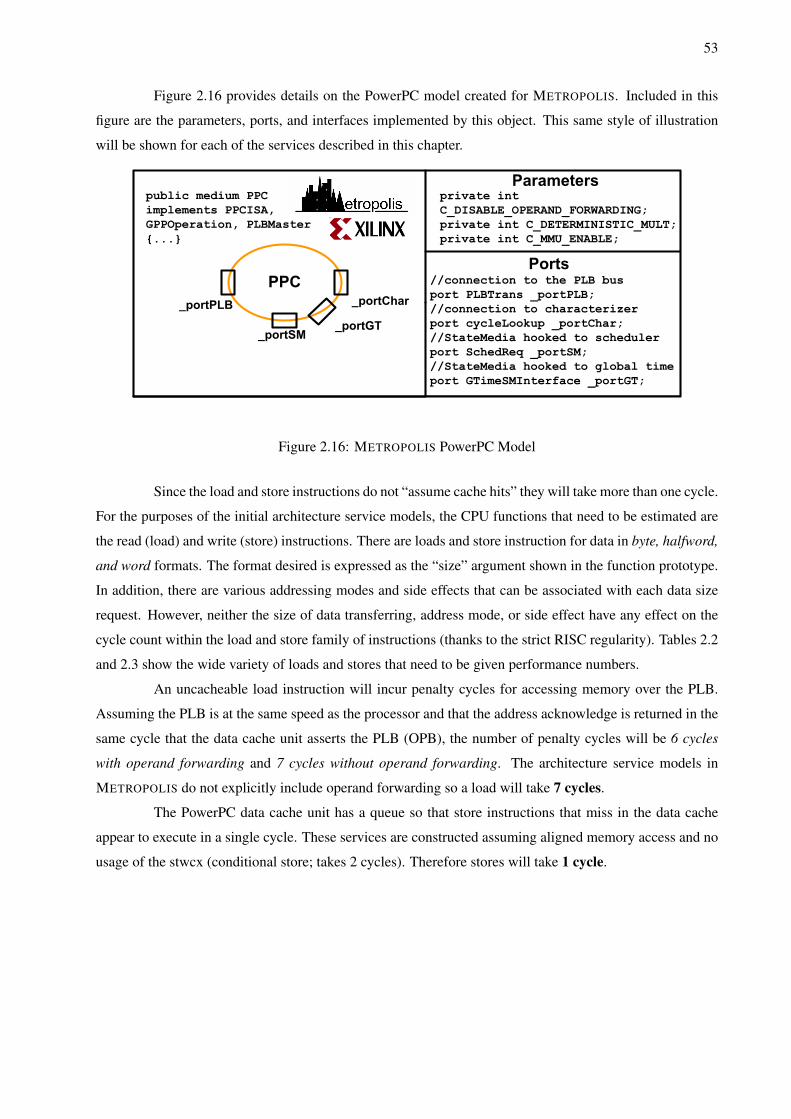
53
Figure 2.16 provides details on the PowerPC model created for METROPOLIS. Included in this
figure are the parameters, ports, and interfaces implemented by this object. This same style of illustration
will be shown for each of the services described in this chapter.
public medium PPC implements PPCISA, GPPOperation, PLBMaster {...}
private int C_DISABLE_OPERAND_FORWARDING;private int C_DETERMINISTIC_MULT;private int C_MMU_ENABLE;
_portPLB
_portSM
_portChar
//connection to the PLB busport PLBTrans _portPLB; //connection to characterizerport cycleLookup _portChar;//StateMedia hooked to schedulerport SchedReq _portSM;//StateMedia hooked to global timeport GTimeSMInterface _portGT;
_portGT
Figure 2.16: METROPOLIS PowerPC Model
Since the load and store instructions do not “assume cache hits” they will take more than one cycle.
For the purposes of the initial architecture service models, the CPU functions that need to be estimated are
the read (load) and write (store) instructions. There are loads and store instruction for data in byte, halfword,
and word formats. The format desired is expressed as the “size” argument shown in the function prototype.
In addition, there are various addressing modes and side effects that can be associated with each data size
request. However, neither the size of data transferring, address mode, or side effect have any effect on the
cycle count within the load and store family of instructions (thanks to the strict RISC regularity). Tables 2.2
and 2.3 show the wide variety of loads and stores that need to be given performance numbers.
An uncacheable load instruction will incur penalty cycles for accessing memory over the PLB.
Assuming the PLB is at the same speed as the processor and that the address acknowledge is returned in the
same cycle that the data cache unit asserts the PLB (OPB), the number of penalty cycles will be 6 cycles
with operand forwarding and 7 cycles without operand forwarding. The architecture service models in
METROPOLIS do not explicitly include operand forwarding so a load will take 7 cycles.
The PowerPC data cache unit has a queue so that store instructions that miss in the data cache
appear to execute in a single cycle. These services are constructed assuming aligned memory access and no
usage of the stwcx (conditional store; takes 2 cycles). Therefore stores will take 1 cycle.
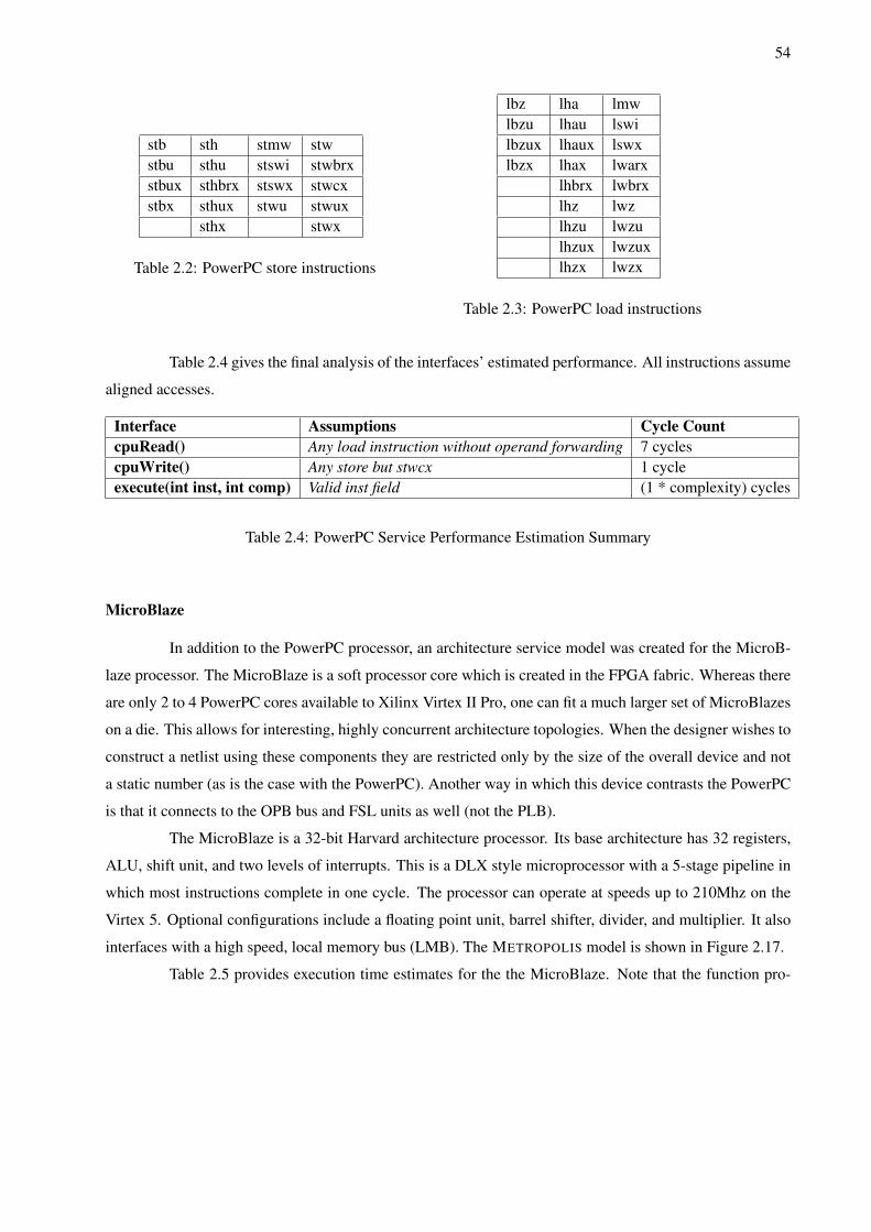
54
stb sth stmw stwstbu sthu stswi stwbrxstbux sthbrx stswx stwcxstbx sthux stwu stwux
sthx stwx
Table 2.2: PowerPC store instructions
lbz lha lmwlbzu lhau lswilbzux lhaux lswxlbzx lhax lwarx
lhbrx lwbrxlhz lwzlhzu lwzulhzux lwzuxlhzx lwzx
Table 2.3: PowerPC load instructions
Table 2.4 gives the final analysis of the interfaces’ estimated performance. All instructions assume
aligned accesses.
Interface Assumptions Cycle CountcpuRead() Any load instruction without operand forwarding 7 cyclescpuWrite() Any store but stwcx 1 cycleexecute(int inst, int comp) Valid inst field (1 * complexity) cycles
Table 2.4: PowerPC Service Performance Estimation Summary
MicroBlaze
In addition to the PowerPC processor, an architecture service model was created for the MicroB-
laze processor. The MicroBlaze is a soft processor core which is created in the FPGA fabric. Whereas there
are only 2 to 4 PowerPC cores available to Xilinx Virtex II Pro, one can fit a much larger set of MicroBlazes
on a die. This allows for interesting, highly concurrent architecture topologies. When the designer wishes to
construct a netlist using these components they are restricted only by the size of the overall device and not
a static number (as is the case with the PowerPC). Another way in which this device contrasts the PowerPC
is that it connects to the OPB bus and FSL units as well (not the PLB).
The MicroBlaze is a 32-bit Harvard architecture processor. Its base architecture has 32 registers,
ALU, shift unit, and two levels of interrupts. This is a DLX style microprocessor with a 5-stage pipeline in
which most instructions complete in one cycle. The processor can operate at speeds up to 210Mhz on the
Virtex 5. Optional configurations include a floating point unit, barrel shifter, divider, and multiplier. It also
interfaces with a high speed, local memory bus (LMB). The METROPOLIS model is shown in Figure 2.17.
Table 2.5 provides execution time estimates for the the MicroBlaze. Note that the function pro-
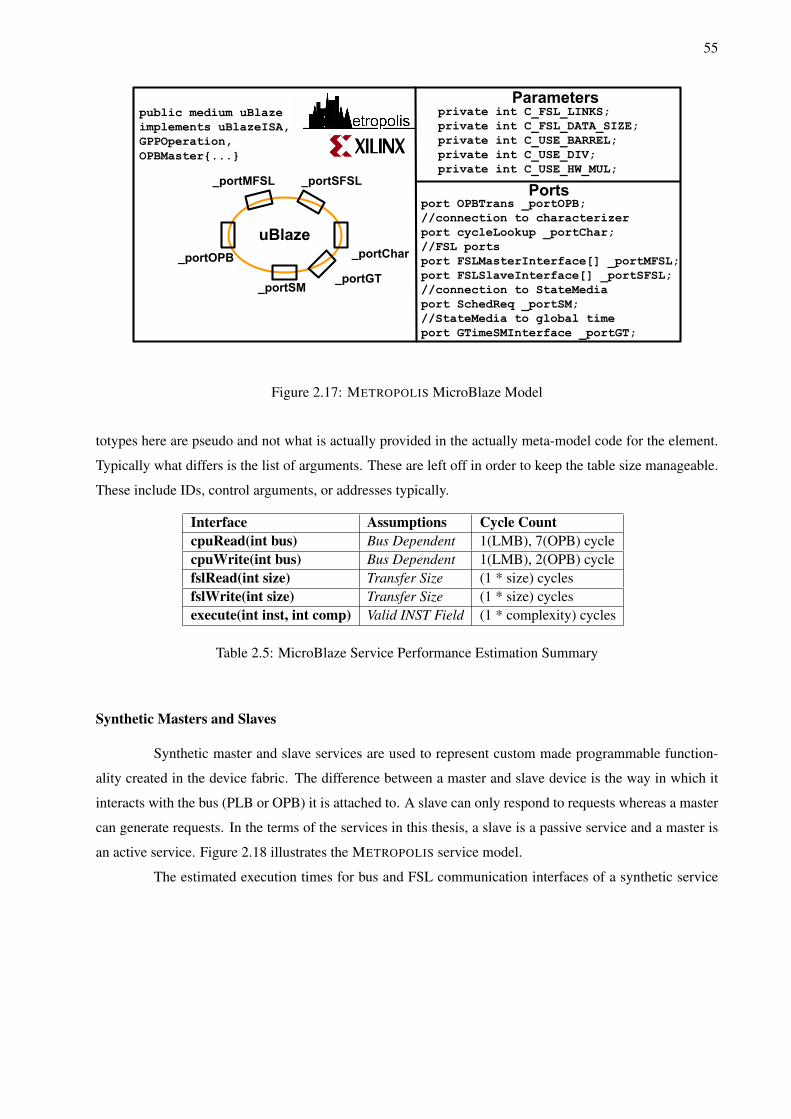
55
public medium uBlaze implements uBlazeISA, GPPOperation, OPBMaster{...}
_portOPB
_portSM
_portChar
port OPBTrans _portOPB; //connection to characterizerport cycleLookup _portChar;//FSL portsport FSLMasterInterface[] _portMFSL;port FSLSlaveInterface[] _portSFSL;//connection to StateMedia port SchedReq _portSM;//StateMedia to global timeport GTimeSMInterface _portGT;
_portGT
_portMFSL _portSFSL
private int C_FSL_LINKS;private int C_FSL_DATA_SIZE;private int C_USE_BARREL;private int C_USE_DIV;private int C_USE_HW_MUL;
Figure 2.17: METROPOLIS MicroBlaze Model
totypes here are pseudo and not what is actually provided in the actually meta-model code for the element.
Typically what differs is the list of arguments. These are left off in order to keep the table size manageable.
These include IDs, control arguments, or addresses typically.
Interface Assumptions Cycle CountcpuRead(int bus) Bus Dependent 1(LMB), 7(OPB) cyclecpuWrite(int bus) Bus Dependent 1(LMB), 2(OPB) cyclefslRead(int size) Transfer Size (1 * size) cyclesfslWrite(int size) Transfer Size (1 * size) cyclesexecute(int inst, int comp) Valid INST Field (1 * complexity) cycles
Table 2.5: MicroBlaze Service Performance Estimation Summary
Synthetic Masters and Slaves
Synthetic master and slave services are used to represent custom made programmable function-
ality created in the device fabric. The difference between a master and slave device is the way in which it
interacts with the bus (PLB or OPB) it is attached to. A slave can only respond to requests whereas a master
can generate requests. In the terms of the services in this thesis, a slave is a passive service and a master is
an active service. Figure 2.18 illustrates the METROPOLIS service model.
The estimated execution times for bus and FSL communication interfaces of a synthetic service
56
public medium
SynthHWTypeS
implements HWOperation
{…}
_portOPB
_portSM
_portChar
port PLBTrans _portPLB;
port OPBTrans _portOPB;
port cycleLookup _portChar;
port FSLMasterInterface[] _portMFSL;
port FSLSlaveInterface[] _portSFSL;
port SchedReq _portSM;
port GTimeSMInterface _portGT;
_portGT
_portMFSL
(master)
_portSFSL
(slave)
private int C_FUNCTION;
private int C_CAPABILITY;
private int C_FSL_LINKS;
Private int C_FSL_DATA_SIZE;
public medium SynthHWTypeM
implements HWOperation {…}
_portPLB
(Slave)
(Master)
Figure 2.18: METROPOLIS Synthetic Master/Slave Model
are the same as the MicroBlaze service costs. The PLB access time for a synthetic service is the same as
the PowerPC service. However, the execution time is a function of what function is being computed, its
complexity, and the port that it is being accessed from. The port being accessed has differing overhead
for a master device as opposed to a slave device. The equation for execution time is inst ∗ complexity +
PortAccessOverhead where 0 < inst ≤ 1,complexity≥ 1, and 2≥ PortAccessOverhead ≥ 0.
CoreConnect Buses
The CoreConnect environment provides three buses. The Processor Local Bus (PLB), the On-
Chip Peripheral Bus (OPB), and the Device Control Register (DCR) Bus. This discussion begins with the
PLB which is where the PowerPC will reside in the majority of designs. The PLB is used to make requests
to memory elements or other peripherals. The OPB which is primarily used with the MicroBlaze, will be
discussed next. The DCR was not modeled because the investigations involved with this thesis did not
require it.
The PLB is the connection provided to the PowerPC cores giving them high speed access to
peripherals. It has separate 32-bit address and 64-bit data buses. It is a fully synchronous bus which supports
multiple master and slave devices. Read and write transfers between master and slave devices occur through
the use of PLB bus transfer signals. Each PLB master has its own address, read-data, and write-data buses.
Slaves have a shared but decoupled interface.
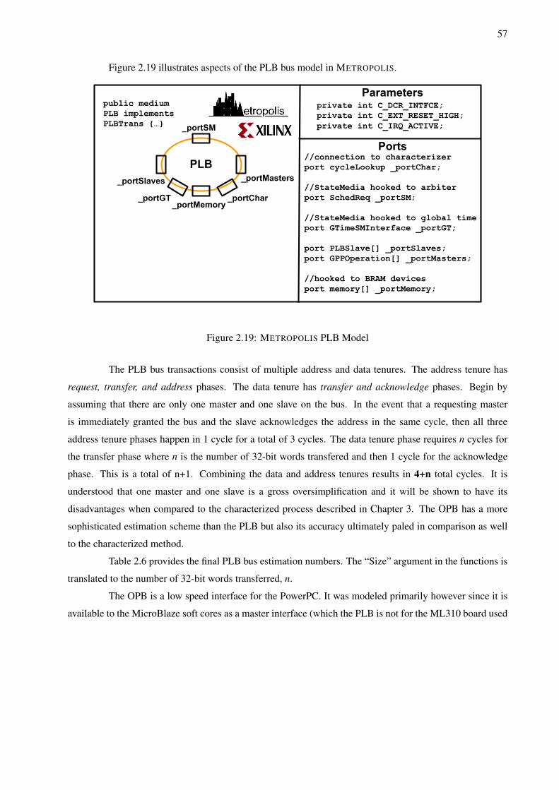
57
Figure 2.19 illustrates aspects of the PLB bus model in METROPOLIS.
_portSlaves _portMasters
_portSM
public medium PLB implements PLBTrans {…}
private int C_DCR_INTFCE;private int C_EXT_RESET_HIGH;private int C_IRQ_ACTIVE;
//connection to characterizerport cycleLookup _portChar;
//StateMedia hooked to arbiterport SchedReq _portSM;
//StateMedia hooked to global timeport GTimeSMInterface _portGT;
port PLBSlave[] _portSlaves;port GPPOperation[] _portMasters;
//hooked to BRAM devicesport memory[] _portMemory;
_portChar_portGT_portMemory
Figure 2.19: METROPOLIS PLB Model
The PLB bus transactions consist of multiple address and data tenures. The address tenure has
request, transfer, and address phases. The data tenure has transfer and acknowledge phases. Begin by
assuming that there are only one master and one slave on the bus. In the event that a requesting master
is immediately granted the bus and the slave acknowledges the address in the same cycle, then all three
address tenure phases happen in 1 cycle for a total of 3 cycles. The data tenure phase requires n cycles for
the transfer phase where n is the number of 32-bit words transfered and then 1 cycle for the acknowledge
phase. This is a total of n+1. Combining the data and address tenures results in 4+n total cycles. It is
understood that one master and one slave is a gross oversimplification and it will be shown to have its
disadvantages when compared to the characterized process described in Chapter 3. The OPB has a more
sophisticated estimation scheme than the PLB but also its accuracy ultimately paled in comparison as well
to the characterized method.
Table 2.6 provides the final PLB bus estimation numbers. The “Size” argument in the functions is
translated to the number of 32-bit words transferred, n.
The OPB is a low speed interface for the PowerPC. It was modeled primarily however since it is
available to the MicroBlaze soft cores as a master interface (which the PLB is not for the ML310 board used
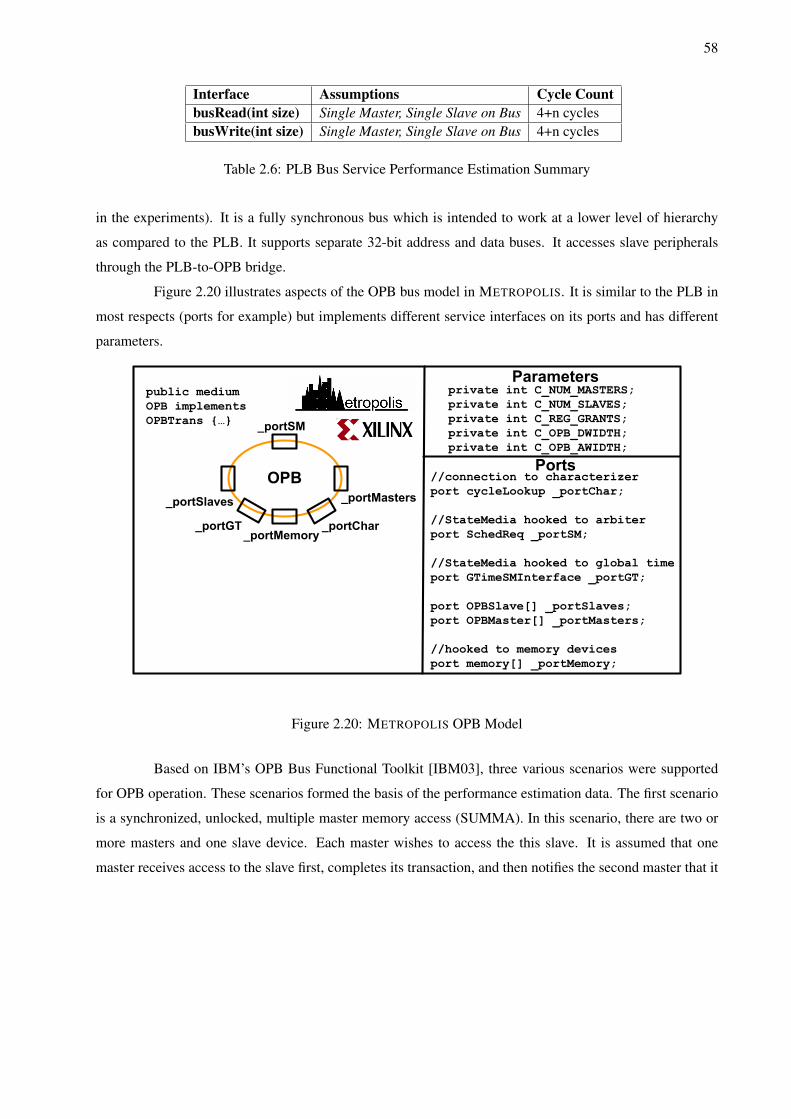
58
Interface Assumptions Cycle CountbusRead(int size) Single Master, Single Slave on Bus 4+n cyclesbusWrite(int size) Single Master, Single Slave on Bus 4+n cycles
Table 2.6: PLB Bus Service Performance Estimation Summary
in the experiments). It is a fully synchronous bus which is intended to work at a lower level of hierarchy
as compared to the PLB. It supports separate 32-bit address and data buses. It accesses slave peripherals
through the PLB-to-OPB bridge.
Figure 2.20 illustrates aspects of the OPB bus model in METROPOLIS. It is similar to the PLB in
most respects (ports for example) but implements different service interfaces on its ports and has different
parameters.
_portSlaves _portMasters
_portSM
public medium OPB implements OPBTrans {…}
private int C_NUM_MASTERS;private int C_NUM_SLAVES;private int C_REG_GRANTS;private int C_OPB_DWIDTH;private int C_OPB_AWIDTH;
//connection to characterizerport cycleLookup _portChar;
//StateMedia hooked to arbiterport SchedReq _portSM;
//StateMedia hooked to global timeport GTimeSMInterface _portGT;
port OPBSlave[] _portSlaves;port OPBMaster[] _portMasters;
//hooked to memory devicesport memory[] _portMemory;
_portChar_portGT_portMemory
Figure 2.20: METROPOLIS OPB Model
Based on IBM’s OPB Bus Functional Toolkit [IBM03], three various scenarios were supported
for OPB operation. These scenarios formed the basis of the performance estimation data. The first scenario
is a synchronized, unlocked, multiple master memory access (SUMMA). In this scenario, there are two or
more masters and one slave device. Each master wishes to access the this slave. It is assumed that one
master receives access to the slave first, completes its transaction, and then notifies the second master that it
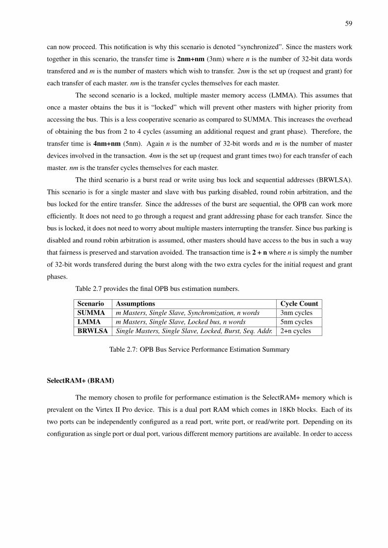
59
can now proceed. This notification is why this scenario is denoted “synchronized”. Since the masters work
together in this scenario, the transfer time is 2nm+nm (3nm) where n is the number of 32-bit data words
transfered and m is the number of masters which wish to transfer. 2nm is the set up (request and grant) for
each transfer of each master. nm is the transfer cycles themselves for each master.
The second scenario is a locked, multiple master memory access (LMMA). This assumes that
once a master obtains the bus it is “locked” which will prevent other masters with higher priority from
accessing the bus. This is a less cooperative scenario as compared to SUMMA. This increases the overhead
of obtaining the bus from 2 to 4 cycles (assuming an additional request and grant phase). Therefore, the
transfer time is 4nm+nm (5nm). Again n is the number of 32-bit words and m is the number of master
devices involved in the transaction. 4nm is the set up (request and grant times two) for each transfer of each
master. nm is the transfer cycles themselves for each master.
The third scenario is a burst read or write using bus lock and sequential addresses (BRWLSA).
This scenario is for a single master and slave with bus parking disabled, round robin arbitration, and the
bus locked for the entire transfer. Since the addresses of the burst are sequential, the OPB can work more
efficiently. It does not need to go through a request and grant addressing phase for each transfer. Since the
bus is locked, it does not need to worry about multiple masters interrupting the transfer. Since bus parking is
disabled and round robin arbitration is assumed, other masters should have access to the bus in such a way
that fairness is preserved and starvation avoided. The transaction time is 2 + n where n is simply the number
of 32-bit words transfered during the burst along with the two extra cycles for the initial request and grant
phases.
Table 2.7 provides the final OPB bus estimation numbers.
Scenario Assumptions Cycle CountSUMMA m Masters, Single Slave, Synchronization, n words 3nm cyclesLMMA m Masters, Single Slave, Locked bus, n words 5nm cyclesBRWLSA Single Masters, Single Slave, Locked, Burst, Seq. Addr. 2+n cycles
Table 2.7: OPB Bus Service Performance Estimation Summary
SelectRAM+ (BRAM)
The memory chosen to profile for performance estimation is the SelectRAM+ memory which is
prevalent on the Virtex II Pro device. This is a dual port RAM which comes in 18Kb blocks. Each of its
two ports can be independently configured as a read port, write port, or read/write port. Depending on its
configuration as single port or dual port, various different memory partitions are available. In order to access
60
the memory, there is one read operation and three write operations (write first, read first, and no change).
Operation is synchronous and behaves like a register in that address and data inputs need to be valid during
a set up time and hold time window prior to a rising edge of a clock edge. Data output changes as a result of
that same clock edge. SelectRAM+ was chosen since it is very easy to profile, prevalent on the device, and
easy to model.
SelectRAM+ is often called block RAM or BRAM because of how it is available in cascaded
blocks along the FPGA configurable logic blocks (CLBs). This makes them available to implement deeper
or wider single- or dual-port memory elements. In the largest Xilinx Virtex II Pro device (XC2VP125) there
are 18 columns of BRAM for a total of 10,008 Kbits.
BRAM interfaces were exported up to the functional model to simplify the creation of basic sys-
tems. Parameters required are the enable (EN), write enable (WE), and Set/Reset (SSR) signals. Also
BRAM was very easy to use in creating actual implementations for comparison with the simulations. Often
times, simple communication with BRAMs made for very effective dataflow systems based on the MicroB-
laze and FSL components.
Figure 2.19 illustrates the BRAM bus model in METROPOLIS.
public medium BRAM implements memory {…}
_portChar _portGT
private int C_MEMSIZE; private int C_PORT_DWIDTH; private int C_PORT_AWIDTH; private int C_NUM_WE;
//connection to global timeport GTimeSMInterface portGT;
//port to the characterizerport cycleLookup portChar;
Figure 2.21: METROPOLIS BRAM Model
The read operation for BRAM uses only one clock edge. If the read address is provided by that
clock edge the stored data is loaded into the output latches after the RAM access interval has elapsed.
The write operation as mentioned could be in one of three forms. The default mode is write first
where the data is written to the memory then that data is stored on the data output (as opposed to read first
where the “old data” is sent to the output while the new data is stored). No change maintains the content of
the output register throughout the the new operation.
In order to get the latency estimates of the memory, one can use estimates from the application
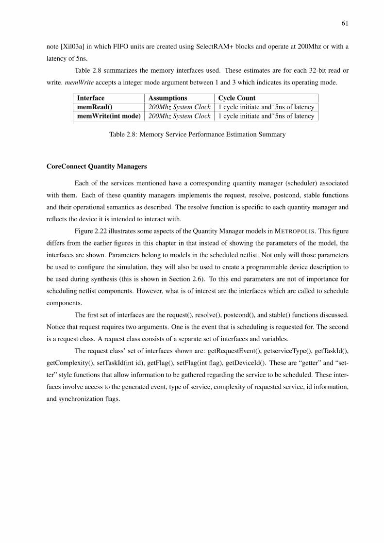
61
note [Xil03a] in which FIFO units are created using SelectRAM+ blocks and operate at 200Mhz or with a
latency of 5ns.
Table 2.8 summarizes the memory interfaces used. These estimates are for each 32-bit read or
write. memWrite accepts a integer mode argument between 1 and 3 which indicates its operating mode.
Interface Assumptions Cycle CountmemRead() 200Mhz System Clock 1 cycle initiate and˜5ns of latencymemWrite(int mode) 200Mhz System Clock 1 cycle initiate and˜5ns of latency
Table 2.8: Memory Service Performance Estimation Summary
CoreConnect Quantity Managers
Each of the services mentioned have a corresponding quantity manager (scheduler) associated
with them. Each of these quantity managers implements the request, resolve, postcond, stable functions
and their operational semantics as described. The resolve function is specific to each quantity manager and
reflects the device it is intended to interact with.
Figure 2.22 illustrates some aspects of the Quantity Manager models in METROPOLIS. This figure
differs from the earlier figures in this chapter in that instead of showing the parameters of the model, the
interfaces are shown. Parameters belong to models in the scheduled netlist. Not only will those parameters
be used to configure the simulation, they will also be used to create a programmable device description to
be used during synthesis (this is shown in Section 2.6). To this end parameters are not of importance for
scheduling netlist components. However, what is of interest are the interfaces which are called to schedule
components.
The first set of interfaces are the request(), resolve(), postcond(), and stable() functions discussed.
Notice that request requires two arguments. One is the event that is scheduling is requested for. The second
is a request class. A request class consists of a separate set of interfaces and variables.
The request class’ set of interfaces shown are: getRequestEvent(), getserviceType(), getTaskId(),
getComplexity(), setTaskId(int id), getFlag(), setFlag(int flag), getDeviceId(). These are “getter” and “set-
ter” style functions that allow information to be gathered regarding the service to be scheduled. These inter-
faces involve access to the generated event, type of service, complexity of requested service, id information,
and synchronization flags.
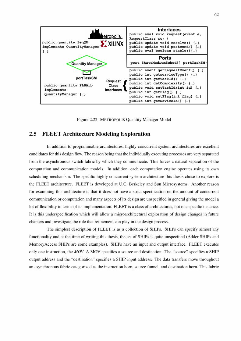
62
public quantity PLBArb
implements
QuantityManager {…}
portTaskSM
public quantity SeqQM
implements QuantityManager
{…}
port StateMediumSched[] portTaskSM;
public eval void request(event e,
RequestClass rc) {
public update void resolve() {…}
public update void postcond() {…}
public eval boolean stable(){…}
public event getRequestEvent() {…}
public int getserviceType() {…}
public int getTaskId() {…}
public int getComplexity() {…}
public void setTaskId(int id) {…}
public int getFlag() {…}
public void setFlag(int flag) {…}
public int getDeviceId() {…}
Quantity Manager
Request
Class
Interfaces
Figure 2.22: METROPOLIS Quantity Manager Model
2.5 FLEET Architecture Modeling Exploration
In addition to programmable architectures, highly concurrent system architectures are excellent
candidates for this design flow. The reason being that the individually executing processes are very separated
from the asynchronous switch fabric by which they communicate. This forces a natural separation of the
computation and communication models. In addition, each computation engine operates using its own
scheduling mechanism. The specific highly concurrent system architecture this thesis chose to explore is
the FLEET architecture. FLEET is developed at U.C. Berkeley and Sun Microsystems. Another reason
for examining this architecture is that it does not have a strict specification on the amount of concurrent
communication or computation and many aspects of its design are unspecified in general giving the model a
lot of flexibility in terms of its implementation. FLEET is a class of architectures, not one specific instance.
It is this underspecification which will allow a microarchitectural exploration of design changes in future
chapters and investigate the role that refinement can play in the design process.
The simplest description of FLEET is as a collection of SHIPs. SHIPs can specify almost any
functionality and at the time of writing this thesis, the set of SHIPs is quite unspecified (Adder SHIPs and
MemoryAccess SHIPs are some examples). SHIPs have an input and output interface. FLEET executes
only one instruction, the MOV. A MOV specifies a source and destination. The “source” specifies a SHIP
output address and the “destination” specifies a SHIP input address. The data transfers move throughout
an asynchronous fabric categorized as the instruction horn, source funnel, and destination horn. This fabric
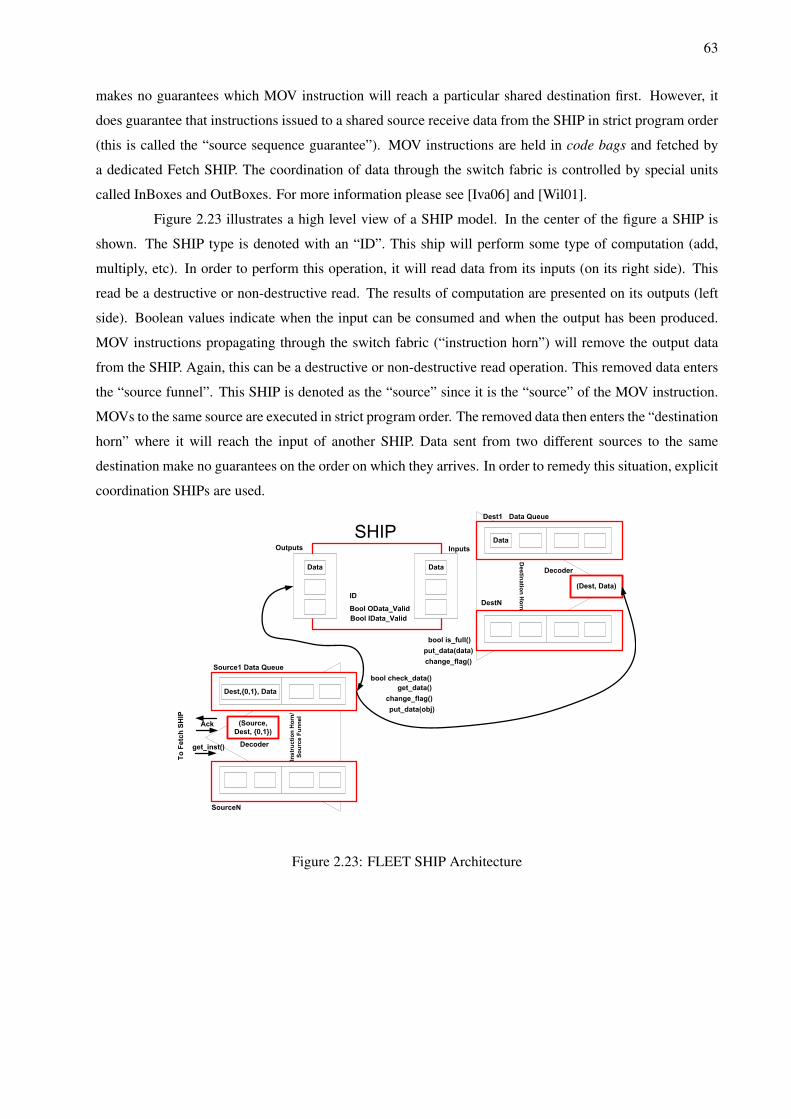
63
makes no guarantees which MOV instruction will reach a particular shared destination first. However, it
does guarantee that instructions issued to a shared source receive data from the SHIP in strict program order
(this is called the “source sequence guarantee”). MOV instructions are held in code bags and fetched by
a dedicated Fetch SHIP. The coordination of data through the switch fabric is controlled by special units
called InBoxes and OutBoxes. For more information please see [Iva06] and [Wil01].
Figure 2.23 illustrates a high level view of a SHIP model. In the center of the figure a SHIP is
shown. The SHIP type is denoted with an “ID”. This ship will perform some type of computation (add,
multiply, etc). In order to perform this operation, it will read data from its inputs (on its right side). This
read be a destructive or non-destructive read. The results of computation are presented on its outputs (left
side). Boolean values indicate when the input can be consumed and when the output has been produced.
MOV instructions propagating through the switch fabric (“instruction horn”) will remove the output data
from the SHIP. Again, this can be a destructive or non-destructive read operation. This removed data enters
the “source funnel”. This SHIP is denoted as the “source” since it is the “source” of the MOV instruction.
MOVs to the same source are executed in strict program order. The removed data then enters the “destination
horn” where it will reach the input of another SHIP. Data sent from two different sources to the same
destination make no guarantees on the order on which they arrives. In order to remedy this situation, explicit
coordination SHIPs are used.
Destination Horn
ID
Bool OData_Valid
Bool IData_Valid
Data
bool is_full()
put_data(data)
Data
Data
(Dest, Data)
Dest1
DestN
Decoder
Data Queue
Instruction Horn/
Source Funnel
Dest,{0,1}, Data
(Source,
Dest, {0,1})
Source1
SourceN
Decoder
Data Queue
bool check_data()
Ack
get_inst()
To Fetch SHIP
put_data(obj)
change_flag()
Outputs Inputs
get_data()
change_flag()
Figure 2.23: FLEET SHIP Architecture
64
The switch fabric can be thought of at the system level as a collection of source and destination
queues (one for each SHIP). In order to replicate its asynchronous nature, a series of handshakes occur in
which local variables are manipulated using “set” and “get” type functions. An example of these functions
are shown in Figure 2.23 as check data(), get data(), change flag(), and put data(obj). The MOV instruction
is an object which begins with the following information: source, destination, copy/move (non-destructive
or not). When it reaches the source, the data is appended and all that is kept is the destination information.
The fact that the switch fabric can be thought of as a set of buffers will be important later in this thesis where
various implementations of these buffers are presented.
Not shown in Figure 2.23 are objects which coordinate the interaction between the switch fabric
and the SHIP. These interfaces are called “inboxes” and “outboxes”. Inboxes and outboxes deal with latching
data as it reaches the ship. These are used to provide a consistent interface to the switch fabric.
For this thesis, SystemC models of FLEET services were created. Specifically the following
services were produced: Fetch SHIP, Adder SHIP, RecordStore SHIP (intermediate storage) , Literal SHIP
(provides static values), and Instruction Memory. Inboxes, Outboxes, and switch fabric (instruction horn,
destination horn, and source funnel) were also created but are not strictly considered services since they are
not exporting their services in such a way that they can be mapped to functional descriptions. This collection
of services is shown in Figure 2.24. In this figure, the interfaces for each service are shown along with what
type of data they operate on.
2.6 Synthesis Path for Architecture Services
One of the goals of the proposed flow presented in this thesis is to find a way to take architecture
service models and produce output which can be used in various synthesis flows. This process has been
termed, “narrowing the gap”. A desirable outcome of the Xilinx modeling effort is the production of a file
for the programmable tool flow which does not suffer from the translation gaps present in the naıve flow.
This process will ensure that the the architecture topology created not only matches that of the model used
in METROPOLIS simulation but also that it has the same parameters which effect the simulation.
Because of the enforcement of parameterized IP like service construction, Xilinx Microprocessor
Hardware Specification (MHS) file generation is automatic. It consists of the following steps which are
illustrated in Figure 2.25:
1. Assemble the scheduled netlist - This step consists of making the connections between architecture
elements the designer is interested in simulating. This is naturally part of the design process and is re-
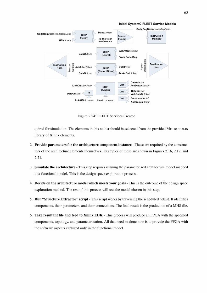
65
Instruction
Memory
SHIP
(Literal)
SHIP
(Fetch)
SHIP
(RecordStore)
SHIP
(Adder)
OB1
IB
OB3
OB2
Instruction
HornSources
Outputs Destination
Horn
Inputs
Desitination
Source
Funnel
DataOut::int
AckAtOut::token
From Code Bag
DataIn::int
AckAtOut::tokenDataOut::int
AckAtIn::token
CodeBagDesIn::codeBagDesc
Which::any
Done::token
To the fetch mechanism
Initial SystemC FLEET Service Models
DataOut::int
AckAtOut::token
LinkOut::boolean
LinkIn::boolean
DataBin::int
DataAin::int
AckDataA::token
AckDataB::token
CommandIn::int
AckComIn::token
CodeBagDesIn::codeBagDesc
Figure 2.24: FLEET Services Created
quired for simulation. The elements in this netlist should be selected from the provided METROPOLIS
library of Xilinx elements.
2. Provide parameters for the architecture component instance - These are required by the construc-
tors of the architecture elements themselves. Examples of these are shown in Figures 2.16, 2.19, and
2.21.
3. Simulate the architecture - This step requires running the parameterized architecture model mapped
to a functional model. This is the design space exploration process.
4. Decide on the architecture model which meets your goals - This is the outcome of the design space
exploration method. The rest of this process will use the model chosen in this step.
5. Run “Structure Extractor” script - This script works by traversing the scheduled netlist. It identifies
components, their parameters, and their connections. The final result is the production of a MHS file.
6. Take resultant file and feed to Xilinx EDK - This process will produce an FPGA with the specified
components, topology, and parameterization. All that need be done now is to provide the FPGA with
the software aspects captured only in the functional model.
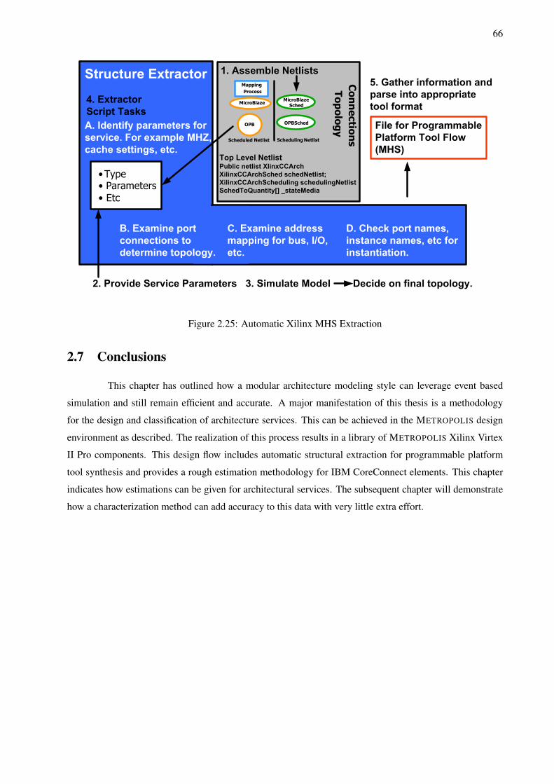
66
Scheduled Netlist Scheduling Netlist
Mapping
Process
MicroBlaze
OPB OPB Sched
MicroBlazeSched
Connections
TopologyA. Identify parameters for
service. For example MHZ,
cache settings, etc.
D. Check port names,
instance names, etc for
instantiation.
5. Gather information and
parse into appropriate
tool format
1. Assemble Netlists
2. Provide Service Parameters 3. Simulate Model Decide on final topology.
4. Extractor
Script Tasks
•Type• Parameters
• Etc
C. Examine address
mapping for bus, I/O,
etc.
B. Examine port
connections to
determine topology.
Top Level NetlistPublic netlist XlinxCCArch
XilinxCCArchSched schedNetlist;
XilinxCCArchScheduling schedulingNetlist
SchedToQuantity[] _stateMedia
File for Programmable
Platform Tool Flow
(MHS)
Figure 2.25: Automatic Xilinx MHS Extraction
2.7 Conclusions
This chapter has outlined how a modular architecture modeling style can leverage event based
simulation and still remain efficient and accurate. A major manifestation of this thesis is a methodology
for the design and classification of architecture services. This can be achieved in the METROPOLIS design
environment as described. The realization of this process results in a library of METROPOLIS Xilinx Virtex
II Pro components. This design flow includes automatic structural extraction for programmable platform
tool synthesis and provides a rough estimation methodology for IBM CoreConnect elements. This chapter
indicates how estimations can be given for architectural services. The subsequent chapter will demonstrate
how a characterization method can add accuracy to this data with very little extra effort.
67
Chapter 3
Architecture Service Characterization
“The first rule of any technology used in a business is that automation applied to an efficientoperation will magnify the efficiency. The second is that automation applied to an inefficientoperation will magnify the inefficiency.” - Bill Gates, Microsoft Co-Founder
In [Ada04], the relative importance of ESL design tasks was explored for a variety of product
scenarios. The design tasks identified are “early software development”, “functional verification”, “perfor-
mance analysis”, and “design space exploration”. Crossing the “methodology gap” introduced in Chapter
1 requires a suitable ESL technology be in place for each of these design tasks. Furthermore, ESL tools
must address the design tasks in a way that matches the designer’s specific product scenario. An ESL solu-
tion for application specific standard products (ASSPs) will differ from the solution for structured ASICs.
Figure 3.1 formulates, as an example, an ESL roadmap to support the transition of RTL designers to ESL.
This illustration is based on Figure 1.2 which illustrated the productivity progress required for ESL adop-
tion. The exact number and sequence of steps varies according to the priorities of a given market segment.
Each technology that is in place is a step up from RTL to ESL and a complete set of steps is required for a
smooth transition. If one or more of the steps are missing, the risk of migration will deter designers that are
not close to their “maximum tolerable design gap”. Designers that reach their maximum tolerance before
the ESL steps are available are in a pathological scenario because their product is no longer cost effective
to develop. Naturally, the steps must also occur in a timely manner or system complexity will overtake
productivity again.
Chapter 2 and this thesis in general deal with the design space exploration step. However this
chapter focuses on one specific step in the transition from RTL to ESL, ESL performance characteriza-
tion (and analysis). ESL performance characterization allows designers to predict whether a given system
architecture can meet a requested level of performance. For this process to be truly useful, performance
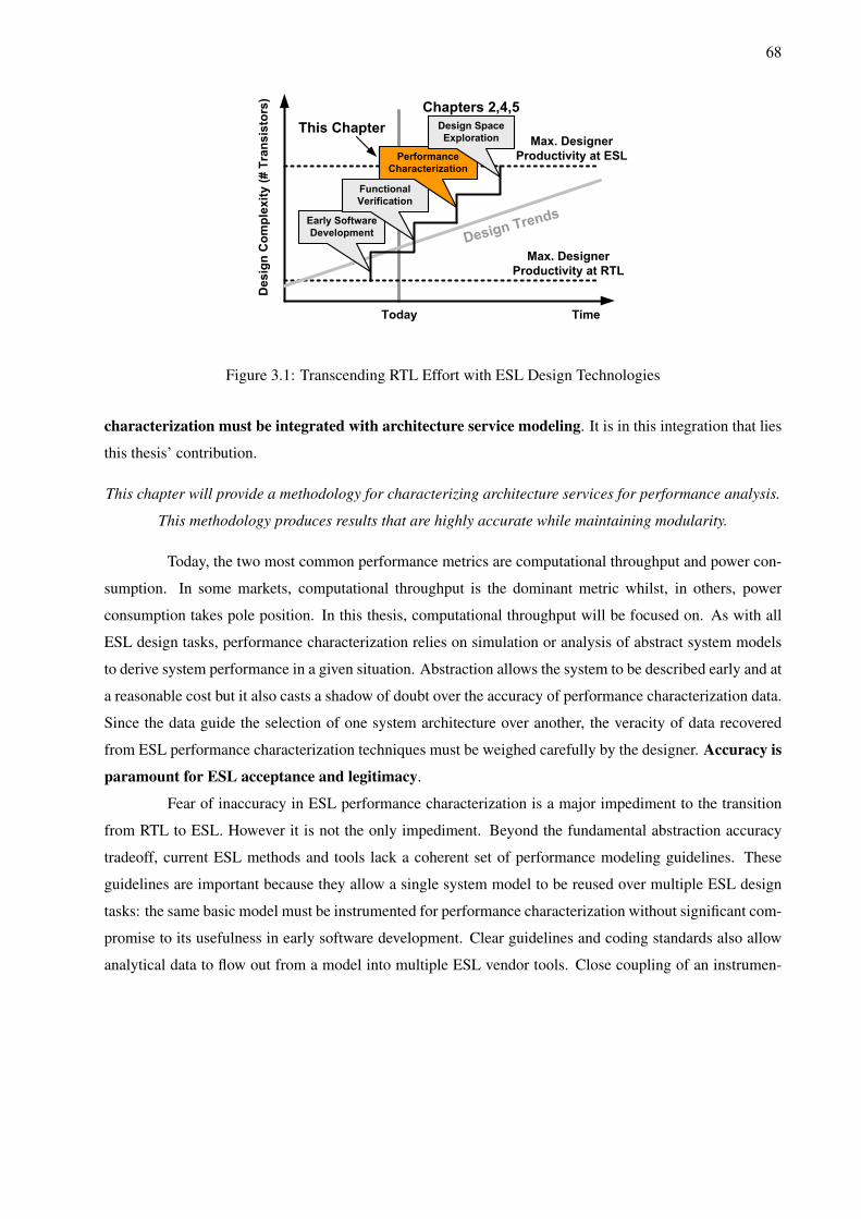
68
Max. Designer
Productivity at ESL
Max. Designer
Productivity at RTLD
esig
n C
om
ple
xity (# T
ransis
tors
)
TimeToday
Early Software
Development
Functional
Verification
Performance
Characterization
This Chapter Design Space
Exploration
Chapters 2,4,5
Design Trends
Figure 3.1: Transcending RTL Effort with ESL Design Technologies
characterization must be integrated with architecture service modeling. It is in this integration that lies
this thesis’ contribution.
This chapter will provide a methodology for characterizing architecture services for performance analysis.
This methodology produces results that are highly accurate while maintaining modularity.
Today, the two most common performance metrics are computational throughput and power con-
sumption. In some markets, computational throughput is the dominant metric whilst, in others, power
consumption takes pole position. In this thesis, computational throughput will be focused on. As with all
ESL design tasks, performance characterization relies on simulation or analysis of abstract system models
to derive system performance in a given situation. Abstraction allows the system to be described early and at
a reasonable cost but it also casts a shadow of doubt over the accuracy of performance characterization data.
Since the data guide the selection of one system architecture over another, the veracity of data recovered
from ESL performance characterization techniques must be weighed carefully by the designer. Accuracy is
paramount for ESL acceptance and legitimacy.
Fear of inaccuracy in ESL performance characterization is a major impediment to the transition
from RTL to ESL. However it is not the only impediment. Beyond the fundamental abstraction accuracy
tradeoff, current ESL methods and tools lack a coherent set of performance modeling guidelines. These
guidelines are important because they allow a single system model to be reused over multiple ESL design
tasks: the same basic model must be instrumented for performance characterization without significant com-
promise to its usefulness in early software development. Clear guidelines and coding standards also allow
analytical data to flow out from a model into multiple ESL vendor tools. Close coupling of an instrumen-
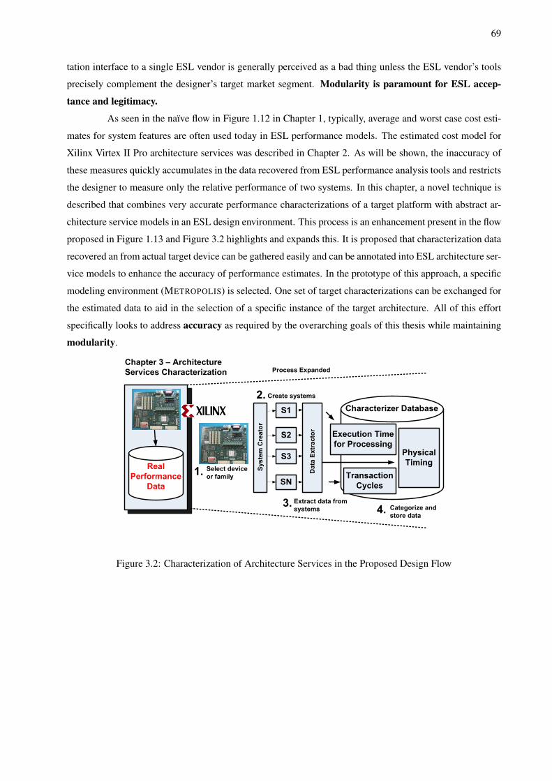
69
tation interface to a single ESL vendor is generally perceived as a bad thing unless the ESL vendor’s tools
precisely complement the designer’s target market segment. Modularity is paramount for ESL accep-
tance and legitimacy.
As seen in the naıve flow in Figure 1.12 in Chapter 1, typically, average and worst case cost esti-
mates for system features are often used today in ESL performance models. The estimated cost model for
Xilinx Virtex II Pro architecture services was described in Chapter 2. As will be shown, the inaccuracy of
these measures quickly accumulates in the data recovered from ESL performance analysis tools and restricts
the designer to measure only the relative performance of two systems. In this chapter, a novel technique is
described that combines very accurate performance characterizations of a target platform with abstract ar-
chitecture service models in an ESL design environment. This process is an enhancement present in the flow
proposed in Figure 1.13 and Figure 3.2 highlights and expands this. It is proposed that characterization data
recovered an from actual target device can be gathered easily and can be annotated into ESL architecture ser-
vice models to enhance the accuracy of performance estimates. In the prototype of this approach, a specific
modeling environment (METROPOLIS) is selected. One set of target characterizations can be exchanged for
the estimated data to aid in the selection of a specific instance of the target architecture. All of this effort
specifically looks to address accuracy as required by the overarching goals of this thesis while maintaining
modularity.
Real
Performance
Data
Chapter 3 – Architecture
Services Characterization
Categorize and
store data
Physical
Timing
Execution Time
for Processing
Transaction
Cycles
Characterizer Database
Select device
or family
Create systems
System Creator
S2
S1
S3
SN
Extract data from
systems
Data Extractor
Process Expanded
Figure 3.2: Characterization of Architecture Services in the Proposed Design Flow
70
3.0.1 Chapter Organization
The remainder of this chapter is organized as follows: first in Section 3.1, the technique’s general
process is discussed along with its set of requirements and assumptions. The next section (3.2) offers more
details on the pre-characterization process by discussing the automatic generation of the group of target
systems. An important part of this discussion is how to automate the extraction of reusable performance
data from the target system’s physical design flow. Section 3.3 provides an example of the characterization
data that can be obtained with this automated method. Storage, organization, and categorization of this data
are discussed next in Sections 3.4 and 3.5. A Motion-JPEG encoder example of pre-characterizing processor
systems on Xilinx Virtex Platform FPGAs is contained in Chapter 5 (along with all design examples). This
chapter concludes by summarizing the results and discussing potential future work.
3.1 Platform Characterization
Platform characterization is the process of systematically measuring a set of properties of a phys-
ical platform or its components. Ultimately, this measurement data will be annotated to ESL architecture
service models of the platform’s components. Subsequent simulations of the now annotated model yield
performance estimates that are correlated to the actual target platform. As such, they are more accurate
than equivalent models annotated with “ballpark” performance metrics. In short, platform characterization
extracts a relevant group of performance measures from the physical implementation of a platform.
For characterization to be applicable to a system design, an appropriate, measurable implemen-
tation of the target platform must already exist. Clearly, ASIC designs are less amenable to this approach
because a suitable implementation of the implementation target is not available early enough in the design
process. Fortunately, programmable platforms based on FPGA technology and ASSP based systems are
common targets for new design starts [Gar08]. Both technologies are amenable to the proposed approach.
In the case of an ASSP, its physical properties and system architecture are fixed at fabrication. For FPGAs,
the physical properties of the platform are fixed at fabrication, but the system architecture is flexible. Clearly
one cannot apply this technique to the designer’s final platform: the system architecture for the designer’s
product has not yet been determined. Instead, it is necessary to pre-characterize a broad set of potential
system architectures that the designer may use. Systems destined for this kind of target require the de-
signer to choose the characterization data that is most representative of the system architecture they intend
to create. Additionally, the designer can explore the effect of different system architectures through their
characterizations.
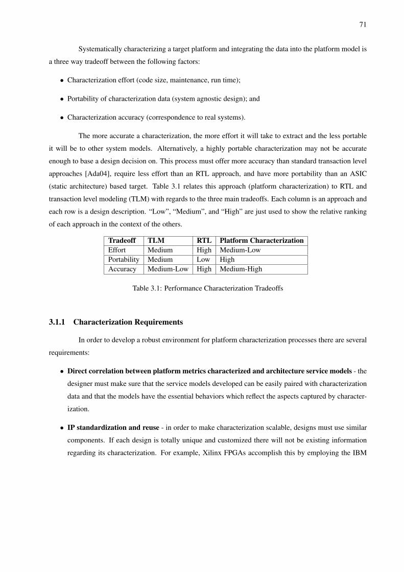
71
Systematically characterizing a target platform and integrating the data into the platform model is
a three way tradeoff between the following factors:
• Characterization effort (code size, maintenance, run time);
• Portability of characterization data (system agnostic design); and
• Characterization accuracy (correspondence to real systems).
The more accurate a characterization, the more effort it will take to extract and the less portable
it will be to other system models. Alternatively, a highly portable characterization may not be accurate
enough to base a design decision on. This process must offer more accuracy than standard transaction level
approaches [Ada04], require less effort than an RTL approach, and have more portability than an ASIC
(static architecture) based target. Table 3.1 relates this approach (platform characterization) to RTL and
transaction level modeling (TLM) with regards to the three main tradeoffs. Each column is an approach and
each row is a design description. “Low”, “Medium”, and “High” are just used to show the relative ranking
of each approach in the context of the others.
Tradeoff TLM RTL Platform CharacterizationEffort Medium High Medium-LowPortability Medium Low HighAccuracy Medium-Low High Medium-High
Table 3.1: Performance Characterization Tradeoffs
3.1.1 Characterization Requirements
In order to develop a robust environment for platform characterization processes there are several
requirements:
• Direct correlation between platform metrics characterized and architecture service models - the
designer must make sure that the service models developed can be easily paired with characterization
data and that the models have the essential behaviors which reflect the aspects captured by character-
ization.
• IP standardization and reuse - in order to make characterization scalable, designs must use similar
components. If each design is totally unique and customized there will not be existing information
regarding its characterization. For example, Xilinx FPGAs accomplish this by employing the IBM
72
CoreConnect bus and the CoreConnect interfaces on the IPs in their Xilinx Embedded Development
Kit (EDK). These are industry standard IP used in embedded system design. This requirement will be
expanded in the next section when extraction is discussed.
• Tool flow for measuring target performance - whichever platform one chooses to model, the actual
target device must have a method and tool flow to gather measures of the characterization metrics.
• System Level Design environment with support for quantity measurements - the framework that
the characterization data is integrated with must support the measurement of quantities (execution
time, power, etc). In addition it must allow for the data used to calculate these quantities come from
an external source.
This chapter will not focus on the details of each requirement. The discussion in this chapter will
describe characterization in the context of the METROPOLIS design environment [Fel03] and Xilinx Virtex
II Pro FPGAs. Other design environments and platform types that meet the requirements above may also be
characterized with this approach.
The next section will discuss how to begin the process of gathering data for use in the characteri-
zation process.
3.2 Extraction of Platform Characterization Data
Extraction of data from the target platform’s physical tool flow is at the heart of this characteriza-
tion methodology. Extraction is a multiphase process concerned with:
• Selecting a programmable platform family - by selecting a family of products in a programmable
product line, one increases the opportunity that the extraction will be portable to other systems. Ide-
ally, the selection of a platform family is done without regard to application domain but, in practice,
this will influence the designer’s decision. An example of a programmable platform family is the
Xilinx Virtex-4 family of platform FPGAs.
• Selecting programmable platform components - the properties of the components will vary de-
pending on the granularity and type of the programmable platform. For example an FPGA could
consist of IP blocks, embedded processing elements, or custom made logic blocks.
• Selecting systems for pre-characterization - from the selected components, assemble a template
system architecture. From this template architecture create many other permutations of this template.
In many cases the permutation of the template architecture is automatic.
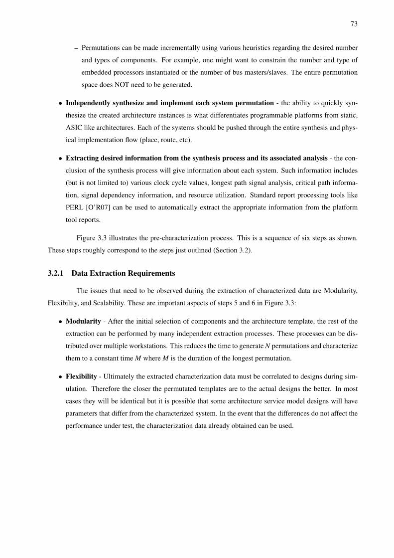
73
– Permutations can be made incrementally using various heuristics regarding the desired number
and types of components. For example, one might want to constrain the number and type of
embedded processors instantiated or the number of bus masters/slaves. The entire permutation
space does NOT need to be generated.
• Independently synthesize and implement each system permutation - the ability to quickly syn-
thesize the created architecture instances is what differentiates programmable platforms from static,
ASIC like architectures. Each of the systems should be pushed through the entire synthesis and phys-
ical implementation flow (place, route, etc).
• Extracting desired information from the synthesis process and its associated analysis - the con-
clusion of the synthesis process will give information about each system. Such information includes
(but is not limited to) various clock cycle values, longest path signal analysis, critical path informa-
tion, signal dependency information, and resource utilization. Standard report processing tools like
PERL [O’R07] can be used to automatically extract the appropriate information from the platform
tool reports.
Figure 3.3 illustrates the pre-characterization process. This is a sequence of six steps as shown.
These steps roughly correspond to the steps just outlined (Section 3.2).
3.2.1 Data Extraction Requirements
The issues that need to be observed during the extraction of characterized data are Modularity,
Flexibility, and Scalability. These are important aspects of steps 5 and 6 in Figure 3.3:
• Modularity - After the initial selection of components and the architecture template, the rest of the
extraction can be performed by many independent extraction processes. These processes can be dis-
tributed over multiple workstations. This reduces the time to generate N permutations and characterize
them to a constant time M where M is the duration of the longest permutation.
• Flexibility - Ultimately the extracted characterization data must be correlated to designs during sim-
ulation. Therefore the closer the permutated templates are to the actual designs the better. In most
cases they will be identical but it is possible that some architecture service model designs will have
parameters that differ from the characterized system. In the event that the differences do not affect the
performance under test, the characterization data already obtained can be used.
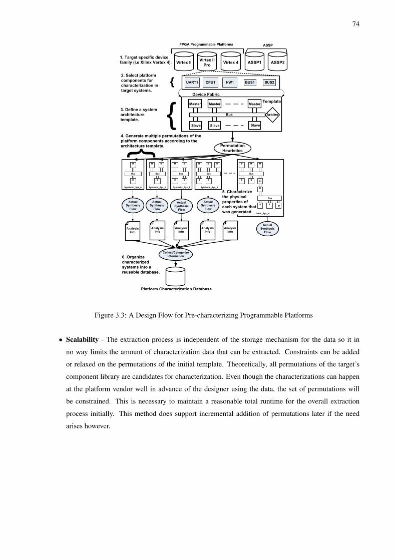
74
Synthetic_Sys_N
Synthetic_Sys_1 Synthetic_Sys_2 Synthetic_Sys_3 Synthetic_Sys_0
text
Master Master Master
Slave Slave Slave
Bus Arbiter
M
S
Bus
M
S
M
Br
S
Bus
M
SBr
M
S
Bus
M
S
MM
S
Bus
M
S
M
S
Bus
MM
S
Bus
1. Target specific device
family (i.e Xilinx Vertex 4).
Device Fabric
CPU1
2. Select platform
components for
characterization in
target systems.
UART1 HW1 BUS1 BUS2
3. Define a system
architecture
template.
4. Generate multiple permutations of the
platform components according to the
architecture template. Permutation
Heuristics
Template
Actual
Synthesis
Flow
Actual
Synthesis
Flow
Actual
Synthesis
Flow
Actual
Synthesis
Flow
Actual
Synthesis
Flow
Analysis
Info
Analysis
Info
Analysis
Info
Analysis
Info
Analysis
Info
Collect/Categorize
Information
Virtex IIVirtex II
ProVirtex 4 ASSP1 ASSP2
FPGA Programmable Platforms ASSP
5. Characterize
the physical
properties of
each system that
was generated.
6. Organize
characterized
systems into a
reusable database.
Platform Characterization Database
Figure 3.3: A Design Flow for Pre-characterizing Programmable Platforms
• Scalability - The extraction process is independent of the storage mechanism for the data so it in
no way limits the amount of characterization data that can be extracted. Constraints can be added
or relaxed on the permutations of the initial template. Theoretically, all permutations of the target’s
component library are candidates for characterization. Even though the characterizations can happen
at the platform vendor well in advance of the designer using the data, the set of permutations will
be constrained. This is necessary to maintain a reasonable total runtime for the overall extraction
process initially. This method does support incremental addition of permutations later if the need
arises however.
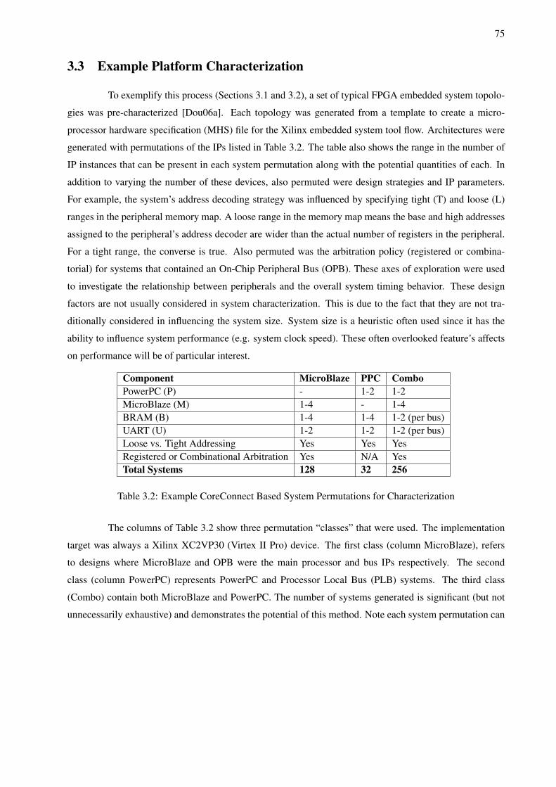
75
3.3 Example Platform Characterization
To exemplify this process (Sections 3.1 and 3.2), a set of typical FPGA embedded system topolo-
gies was pre-characterized [Dou06a]. Each topology was generated from a template to create a micro-
processor hardware specification (MHS) file for the Xilinx embedded system tool flow. Architectures were
generated with permutations of the IPs listed in Table 3.2. The table also shows the range in the number of
IP instances that can be present in each system permutation along with the potential quantities of each. In
addition to varying the number of these devices, also permuted were design strategies and IP parameters.
For example, the system’s address decoding strategy was influenced by specifying tight (T) and loose (L)
ranges in the peripheral memory map. A loose range in the memory map means the base and high addresses
assigned to the peripheral’s address decoder are wider than the actual number of registers in the peripheral.
For a tight range, the converse is true. Also permuted was the arbitration policy (registered or combina-
torial) for systems that contained an On-Chip Peripheral Bus (OPB). These axes of exploration were used
to investigate the relationship between peripherals and the overall system timing behavior. These design
factors are not usually considered in system characterization. This is due to the fact that they are not tra-
ditionally considered in influencing the system size. System size is a heuristic often used since it has the
ability to influence system performance (e.g. system clock speed). These often overlooked feature’s affects
on performance will be of particular interest.
Component MicroBlaze PPC ComboPowerPC (P) - 1-2 1-2MicroBlaze (M) 1-4 - 1-4BRAM (B) 1-4 1-4 1-2 (per bus)UART (U) 1-2 1-2 1-2 (per bus)Loose vs. Tight Addressing Yes Yes YesRegistered or Combinational Arbitration Yes N/A YesTotal Systems 128 32 256
Table 3.2: Example CoreConnect Based System Permutations for Characterization
The columns of Table 3.2 show three permutation “classes” that were used. The implementation
target was always a Xilinx XC2VP30 (Virtex II Pro) device. The first class (column MicroBlaze), refers
to designs where MicroBlaze and OPB were the main processor and bus IPs respectively. The second
class (column PowerPC) represents PowerPC and Processor Local Bus (PLB) systems. The third class
(Combo) contain both MicroBlaze and PowerPC. The number of systems generated is significant (but not
unnecessarily exhaustive) and demonstrates the potential of this method. Note each system permutation can
76
be characterized independently and hence, each job can be farmed out to a network of workstations. For
reference, the total runtime to characterize the largest “Combo” system with Xilinx Platform Studio 6.2i on
a 3GHz Xeon Windows machine with 1 GB of memory was 15 minutes. The physical design tools were run
with the “high effort” option and a User Constraint File (UCF) that attempts to maximize the system clock
frequency. An observation of the characterization data shows that as resource usage increases (measured
by FPGA slice count; a slice contains two 4-input function generators, carry logic, arithmetic logic gates,
muxes, and two storage elements) the overall system clock frequency decreases. Figure 3.4 shows a graph of
sample Combo systems, their size, and reported performance. Nested loops of each IP were used to generate
the system permutations, giving the systems generated predictable increases in area and complexity. The
major, periodic increase in area is as anticipated and indicates that a MicroBlaze processor was added to
the system topology and all other peripheral IPs were reset to their lowest number. Note that the graph’s
performance trace is neither linear nor monotonic. Often area is constant while frequency changes
drastically. This phenomenon prevents area based frequency estimations. The relationship between the
system’s area utilization and performance is complex, showing that building a static model is difficult, if at
all possible, and confirming the hypothesis that actual characterization can provide more accurate results.
Slice Count Frequency
0
1000
2000
3000
4000
1 4 7 10 13 16 19 22 25 28 31 34 37 40 43 46 49 52 55 58 61 64Samples
0
20
40
60
80
100
120
140
High Spikes in Adjacent
(Similar) Samples
Decreasing but not
monotonic or linear
Area Measure Often Plateaus
Added BRAM -1s
Added uBlaze – 2s
Increasing
System
Complexity
1 2 111 2 2
(Area)
(Performance)
Periodic Changes
Figure 3.4: Combo Systems Resource Usage and Performance
Table 3.3 highlights an interesting portion of the data collected in the PowerPC class. Each row is
a PPC system instance: the leftmost columns show the specific IP configuration for the system ((P)owerPC,
(B)RAM, and (U)ART) and the remaining columns show area usage (slice count), max frequency, and the
% change (∆) between the previous system configuration (representing potentially a small change to the
system). This thesis contends that a difference of 10% is noteworthy and 15% is equivalent to a device
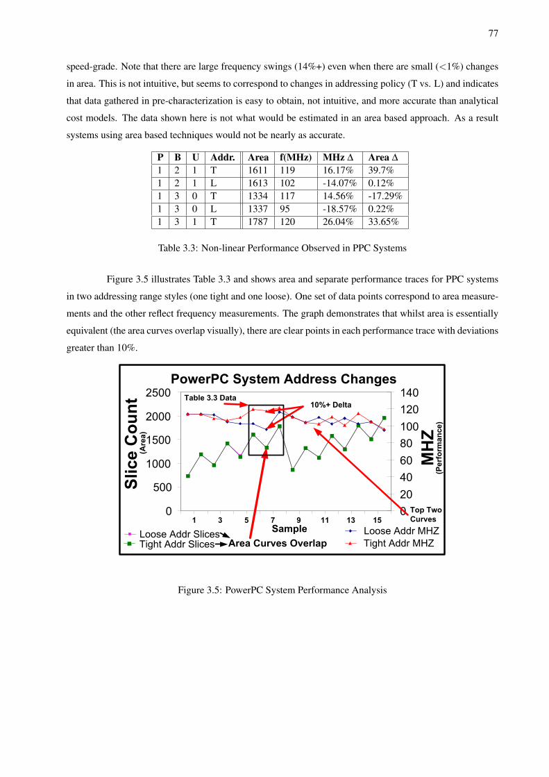
77
speed-grade. Note that there are large frequency swings (14%+) even when there are small (<1%) changes
in area. This is not intuitive, but seems to correspond to changes in addressing policy (T vs. L) and indicates
that data gathered in pre-characterization is easy to obtain, not intuitive, and more accurate than analytical
cost models. The data shown here is not what would be estimated in an area based approach. As a result
systems using area based techniques would not be nearly as accurate.
P B U Addr. Area f(MHz) MHz ∆ Area ∆
1 2 1 T 1611 119 16.17% 39.7%1 2 1 L 1613 102 -14.07% 0.12%1 3 0 T 1334 117 14.56% -17.29%1 3 0 L 1337 95 -18.57% 0.22%1 3 1 T 1787 120 26.04% 33.65%
Table 3.3: Non-linear Performance Observed in PPC Systems
Figure 3.5 illustrates Table 3.3 and shows area and separate performance traces for PPC systems
in two addressing range styles (one tight and one loose). One set of data points correspond to area measure-
ments and the other reflect frequency measurements. The graph demonstrates that whilst area is essentially
equivalent (the area curves overlap visually), there are clear points in each performance trace with deviations
greater than 10%.
1 3 5 7 9 11 13 15
Sample
10%+ Delta
Area Curves Overlap
Table 3.3 Data
Top Two
Curves
(Area)
(Performance)
Figure 3.5: PowerPC System Performance Analysis
78
3.4 Organization of Platform Characterization Data
The organization of the raw, extracted data is the process of categorizing the information in such
a way that system simulation remains efficient, data remains portable, and flexible data interactions can be
explored. This is a very important part of the characterization process and if a poor job is done in this stage,
many of the benefits of the previous efforts will be lost. This is an aspect of step 6 in Figure 3.3. More
concisely the goals are thus:
• Maintain system efficiency - if the simulation performance of the system using estimated data (a
naıve method) is PE and the performance of the system using characterized data (the proposed method)
is PC, the following relation must hold, PC ≥ PE . Performance in this case is a measure of simula-
tion effort or cycles consumed which directly affect the execution time of the simulation or runtime
memory requirement (higher performance results in lower execution time or lower runtime memory
requirement).
• Portable Data - in order to reuse data, it must be stored in such a way that it is maximally portable
amongst various models. This requires three things: 1) A standard interface for accessing the stored
data 2) A common data format for the stored data and 3) The ability for the data set to grow over time.
• Flexible Data Interaction - data interaction refers to the ability to allow many ways in which data
can interact in order to give information regarding the performance of the simulation. For example
if data regarding transactions per instruction can be combined with information regarding cycles per
transaction one can determine the cycles per instruction. Another example is that if Transaction1 can
use signals S1 or S2 and it is known that S1 resides along a longer path than S2, Transaction1 can
utilize S2 for greater performance. It is best to place no restriction on data interaction in so much as it
does not conflict with any of the other characterization goals.
3.4.1 Data Categorization
With the goals defined for “characterization data organization” the second aspect that must be
determined is how data is categorized. Data can be categorized in many ways depending on what is be-
ing modeled. For the sake of this discussion, it will be in the context of what is required typically for
programmable architecture service models of embedded systems. To this end there are three categories:
• Physical Timing - this information details the physical time for signals to propagate through a sys-
tem. Typically this information is gathered via techniques such as static timing analysis or other
79
combinational or sequential logic design techniques to determine clock cycle or other signal delays.
• Transaction Timing - this information is a unit of measure which details the latency or stages of
a transaction. A transaction is an interaction between computational units in point to point manner
or through other communication mechanisms (buses, switches, etc). This could be a cycle count in
reference to a particular global clock which determines the overall speed of the system. Or it could
alternatively be an asynchronous measure.
• Computation Timing - this information is regarding the computation time taken by a specific com-
putation unit. This could be both HW and/or SW based routines. For example it could be a cycle
count given by the time a HW unit (Adder, Shifter, etc) takes to complete its operation. Alternately
it could be the cycle time taken by a particular software routine (Discreet Cosine Transform perhaps)
running on a particular embedded processor.
These three areas interact to give estimated performance for a system under simulation. The
following example (Table 3.4) shows how all three areas can be used along with their ability to flexibility
interact to provide performance analysis:
Instruction Timing Categorization Performance Implicationread(0x64, 10B) Transaction - 1 cycle/Byte 10 cyclesexecute(FFT) Computation - FFT 5 Cycles 5 cycleswrite(0x78, 20B) Transaction - 2 cycles/Byte 40 cyclesTotal Cycles Physical - 1cycle/10ns 550ns
Table 3.4: Sample Simulation Using Characterization Data
The leftmost column provides three different instructions. The center column gives the charac-
terization of each instruction and what category it falls under. The rightmost column gives the resultant
performance implication given the instruction and its characterization. The final row illustrates the execu-
tion time of this sequence of instructions given the physical time of one execution cycle.
3.4.2 Data Storage Structure
Finally, it must be decided what actual structure will hold the now categorized, characterized data.
The primary concerns are related to the goals initially mentioned in this chapter regarding portability and
efficiency. This should be a structure that can grow to accommodate more entries. Ultimately what structure
will be used is determined by which system level design environments are intended to be used. However the
follow issues should be considered:
80
• What is the overhead associated with accessing (reading) the data?
• What is the overhead associated with storing (writing) the data? Both this and the reading overhead
are affected by code size and complexity and ultimately affect simulation speed.
• Can data be reorganized incrementally? This is of use if new data is added or the categorization
mechanism changes.
• Can data be quickly sorted? Searched? This can increase the speed of access and allows exotic
relationships between data elements and their use.
More specifics on data structures for characterization data will be touched on in the next section
when specific example executions are discussed. For now this thesis leaves the reader with an illustration of
an abstract structure in Figure 3.6. The left hand side of the illustration shows the data categorization and in
which stage of the design flow that data is generated. Shown are the three types of data categories as well
as where that data is collected. Notice that each element is connected to the others, illustrating that they
should be flexible in their interaction. Also there should be an input interface (to enter data), as well as an
output interface to retrieve the data. The right hand side shows a sample entry in the data storage structure
where each system categorized has its own index and may have independent or shared entries in the storage
structure. With each index there is associated physical timing, computation timing, and transaction timing
data. This data can be shared or be unique to a particular index. Additionally each index is not required to
have an explicit entry for each category and can utilize a globally stored default value.
3.5 Integration of Platform Characterization and Architectural Services
Once the data has been extracted and organized it now must be integrated into a system level
design environment for simulation. The following discussion will highlight the key issues associated with
this integration and provide an example of each in the METROPOLIS environment.
• Separation of architecture models and their scheduling - this requirement allows for the data struc-
ture containing the extracted data to be independently added and modified apart from the actual sys-
tem.
– In METROPOLIS, architecture models are a combination of two netlists (as described in Chapter
2). The first netlist is called the scheduled netlist and contains the topology and components
that make the architecture instance (CPUs, BUS, etc). The other netlist is the scheduling netlist
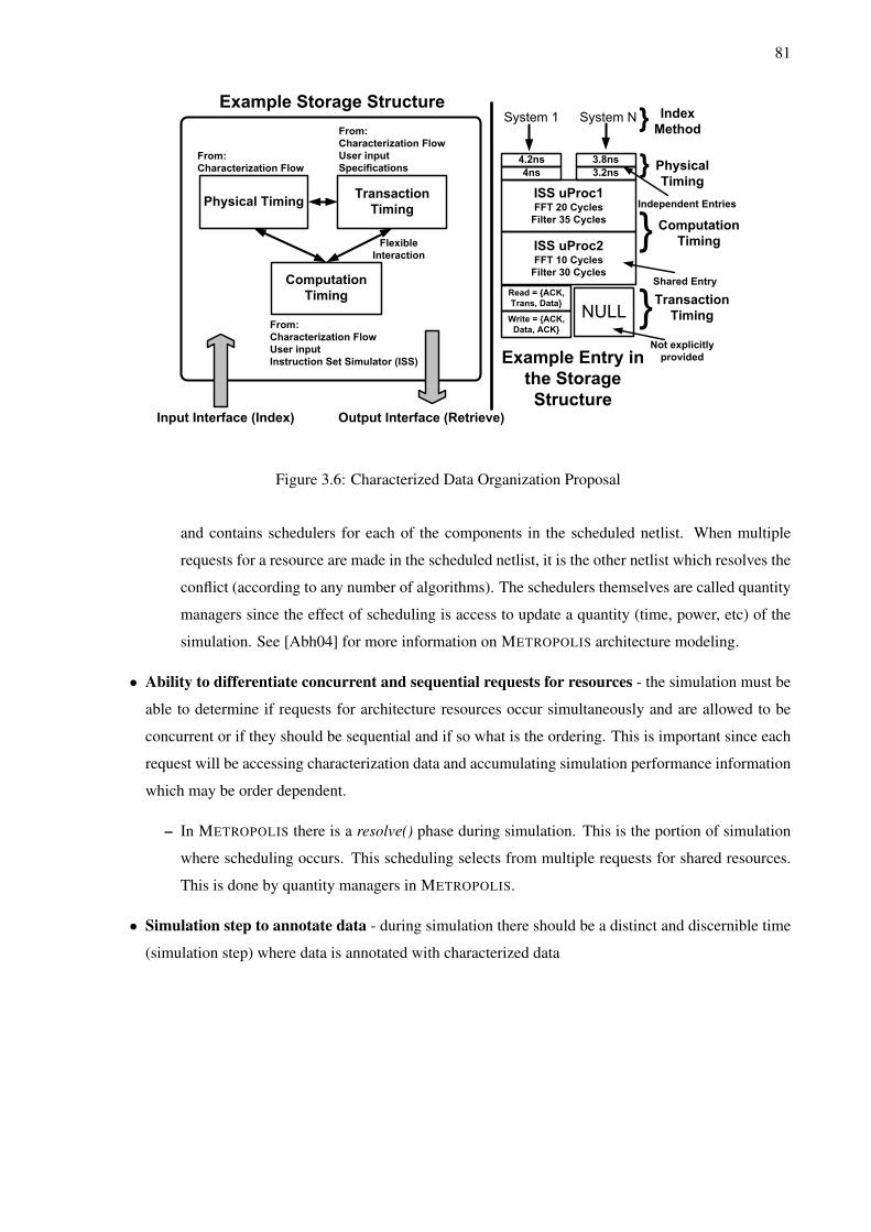
81
Physical TimingTransaction
Timing
Computation
Timing
4.2ns 3.8ns
4ns 3.2ns
ISS uProc1FFT 20 Cycles
Filter 35 Cycles
ISS uProc2FFT 10 Cycles
Filter 30 Cycles
Read = {ACK,
Trans, Data}
Write = {ACK,
Data, ACK}
Physical
Timing
Index
Method
Computation
Timing
Transaction
Timing
From:
Characterization Flow
From:
Characterization Flow
User input
Specifications
From:
Characterization Flow
User input
Instruction Set Simulator (ISS)
Input Interface (Index) Output Interface (Retrieve)
Flexible
Interaction
Shared Entry
Not explicitly
provided
Independent Entries
Figure 3.6: Characterized Data Organization Proposal
and contains schedulers for each of the components in the scheduled netlist. When multiple
requests for a resource are made in the scheduled netlist, it is the other netlist which resolves the
conflict (according to any number of algorithms). The schedulers themselves are called quantity
managers since the effect of scheduling is access to update a quantity (time, power, etc) of the
simulation. See [Abh04] for more information on METROPOLIS architecture modeling.
• Ability to differentiate concurrent and sequential requests for resources - the simulation must be
able to determine if requests for architecture resources occur simultaneously and are allowed to be
concurrent or if they should be sequential and if so what is the ordering. This is important since each
request will be accessing characterization data and accumulating simulation performance information
which may be order dependent.
– In METROPOLIS there is a resolve() phase during simulation. This is the portion of simulation
where scheduling occurs. This scheduling selects from multiple requests for shared resources.
This is done by quantity managers in METROPOLIS.
• Simulation step to annotate data - during simulation there should be a distinct and discernible time
(simulation step) where data is annotated with characterized data

82
– METROPOLIS is an event based framework which generates events in response to functional
stimulus. These events are easily isolated and augmented with information from characterization
during scheduling (with the request() interface). This annotated data is stored in the event’s
“value” set. Events are defined as demonstrated by the tagged-signal model of [Edw98].
The overall message of this integration discussion is that once the data is ready to be integrated
into the design environment 1) it must be able to be added non-destructively 2) it must be able to augment
existing simulation information detailing performance 3) the simulation must be able to correctly recognize
concurrent and sequential interactions/requests for the characterized data.
3.5.1 Sample Annotation Semantics
This final section will demonstrate an example execution of a system integrated with the charac-
terized data. This will be based on the METROPOLIS design environment. In this case, the structure holding
the data is a hash table-like structure indexed by information regarding the topology of the system. Figure
3.7 illustrates these steps in METROPOLIS. Each step in the figure corresponds to a step below.
1. An active METROPOLIS architecture thread generates an event, e. This event represents a request
for a service. This event will have been generated by a functional model mapped to this architecture
needing a service (CPU, BUS, etc). This event can represent a transaction or computation request. In
the case of the figure, the event is generated by a thread.serviceRead() interface call.
2. The service will make a request to its scheduler, with the request(e) method. This passes the request
from the scheduled netlist to the scheduling netlist where e joins a list of pending events. While this
event is waiting scheduling, the task that generated it remains blocked (unable to proceed). In the
figure this is the serviceScheduler.request(e) call.
3. Once all events that can be generated for this simulation step have been generated, the simulation
proceeds to a resolve() phase where scheduling decisions (algorithms vary depending on the service
they schedule) are made which remove select events from the pending lists. The figure illustrates this
in the scheduling netlist’s serviceScheduler.resolve(e) object call.
4. serviceScheduler.Annotate(e) selects events by indexing the characterized database according to event
information. In practice more than just the event is passed. In addition a “request class” is passed also
to provide information for indexing the database. This allows access to simulation quantities (like
simulation global time) which can now be influenced by annotated events. Note that this requires no
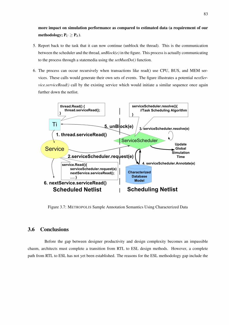
83
more impact on simulation performance as compared to estimated data (a requirement of our
methodology; PC ≥ PE).
5. Report back to the task that it can now continue (unblock the thread). This is the communication
between the scheduler and the thread, unBlock(e) in the figure. This process is actually communicating
to the process through a statemedia using the setMustDo() function.
6. The process can occur recursively when transactions like read() use CPU, BUS, and MEM ser-
vices. These calls would generate their own sets of events. The figure illustrates a potential nextSer-
vice.serviceRead() call by the existing service which would initiate a similar sequence once again
further down the netlist.
thread.Read() {thread.serviceRead();
}
Characterized
Database
Model
Update
Global
Simulation
Time
service.Read(){
serviceScheduler.request(e)
nextService.serviceRead();
…. }
3. serviceScheduler.resolve(e)
4. serviceScheduler.Annotate(e)
serviceScheduler.resolve(){
//Task Scheduling Algorithm
}
Figure 3.7: METROPOLIS Sample Annotation Semantics Using Characterized Data
3.6 Conclusions
Before the gap between designer productivity and design complexity becomes an impassible
chasm, architects must complete a transition from RTL to ESL design methods. However, a complete
path from RTL to ESL has not yet been established. The reasons for the ESL methodology gap include the

84
difficulty of isolating a set of design technologies that solve ESL design problems for the diverse range of
system types. Designers desirous of ESL performance analysis tools are also wary of the accuracy of the
data they can recover from existing tools and models.
In this chapter, an ESL performance analysis technology for programmable platforms was pre-
sented. This approach united characterizations of actual platforms with abstract designer model simula-
tions. The result is an integrated approach to ESL performance modeling that increases the accuracy of
performance estimates. This use of METROPOLIS quantity managers also eases design space exploration by
separating the architectural models of a system from the specific timing model used during system simula-
tion.
Future efforts with system level pre-characterization will begin with a deeper exploration of the
tradeoff between accuracy and a given system model’s level of abstraction. Additionally, formal techniques
can be applied to analyze the bounds of our approach which is currently simulation based.
With both the modeling and characterization of programmable architecture models described. The
next chapter will explore how one can verify properties of these models as they are successively refined from
abstract specifications to actual implementations.
85
Chapter 4
System Level Service Refinement
“Program construction consists of a sequence of refinement steps.” - Niklaus Wirth, Designerof Pascal
Increasing abstraction as shown in Chapters 1 and 2 is a powerful tool in the fight against in-
creased complexity. Platform-Based design explicitly accommodates various levels of abstraction in what
has been termed, “the fractal nature” of the design process [Kur00]. This technique is particularly useful
for architectural servicesand the platforms that result when functional descriptions are mapped to those ser-
vices. Working at various levels of abstraction is useful also in various synthesis situations. For example,
one may want to work at various abstraction levels for the purposes of optimization. Logic minimization
of a gate level netlist as opposed to a more structural netlist is an opportunity for optimization. Analysis of
design decisions during design space exploration, design transformation from one model of computation to
another, or the introduction of physical and implementation concerns, such as wire delays, are all additional
reasons for abstraction. When deciding upon the initial abstraction level or the move to another abstraction
level, it becomes critical that one can ensure that newly introduced models correspond to their more or less
abstract counterparts. Therefore three issues become paramount:
1. What is the behavior that should be required to correspond between the abstract and refined systems?
2. How can that behavior be captured efficiently and formally?
3. How can behaviors once captured be compared?
This chapter will identify three strategies to classify, capture, and verify the behavior of system level
architecture service model. The verification process will be involved in demonstrating that two systems at
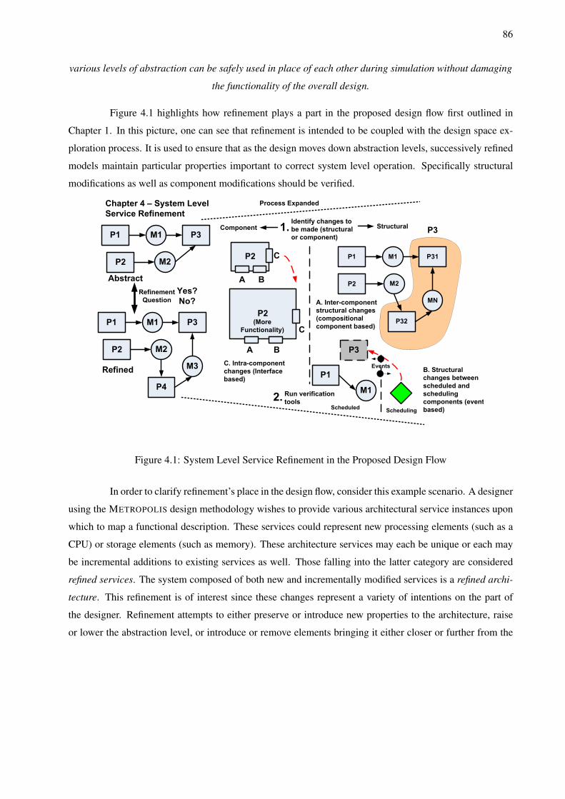
86
various levels of abstraction can be safely used in place of each other during simulation without damaging
the functionality of the overall design.
Figure 4.1 highlights how refinement plays a part in the proposed design flow first outlined in
Chapter 1. In this picture, one can see that refinement is intended to be coupled with the design space ex-
ploration process. It is used to ensure that as the design moves down abstraction levels, successively refined
models maintain particular properties important to correct system level operation. Specifically structural
modifications as well as component modifications should be verified.
Identify changes to
be made (structural
or component)
Process ExpandedChapter 4 – System Level
Service Refinement
P1
P2
P3M1
M2
P1
P2
P3M1
M2
P4
M3
Abstract
Refined
Yes?
No?
P1
P2
P31M1
M2
P32
MN
P3StructuralComponent
A. Inter-component
structural changes
(compositional
component based)
Run verification
tools
B. Structural
changes between
scheduled and
scheduling
components (event
based)
P1
M1
ScheduledScheduling
P3
C. Intra-component
changes (Interface
based)
P2
A
C
B
P2
A
C
B
(More
Functionality)
Events
Refinement
Question
Figure 4.1: System Level Service Refinement in the Proposed Design Flow
In order to clarify refinement’s place in the design flow, consider this example scenario. A designer
using the METROPOLIS design methodology wishes to provide various architectural service instances upon
which to map a functional description. These services could represent new processing elements (such as a
CPU) or storage elements (such as memory). These architecture services may each be unique or each may
be incremental additions to existing services as well. Those falling into the latter category are considered
refined services. The system composed of both new and incrementally modified services is a refined archi-
tecture. This refinement is of interest since these changes represent a variety of intentions on the part of
the designer. Refinement attempts to either preserve or introduce new properties to the architecture, raise
or lower the abstraction level, or introduce or remove elements bringing it either closer or further from the

87
requirements of synthesis. Due to the effort often associated with creating entirely new models, refinements
are often the most common architecture service modifications. Target architectures tend to be a family of
architectures as opposed to entirely new designs. Additionally, testing effort is very valuable and it is desir-
able to repeat as little of this as possible when designing new systems. It is with all these factors in mind
that this thesis examines three methodologies in which to introduce, categorize, create, and test architecture
service refinements. Ultimately I will provide the results of these methodologies in Chapter 5.
4.0.1 Chapter Organization
Before beginning any discussion, Section 4.1 will provide the required background and definitions.
This section is followed by an overview and classification of related work in Section 4.2
The remaining organization of this chapter is such that the reader is introduced to the three re-
finement methods in order of ascending specificity. In Section 4.3 an event based structure for refinement
in illustrated. This method uses events to define system behavior and demonstrates how properties can be
defined over these events. Section 4.4 builds on the previous section by demonstrating how traditional in-
terface based refinement techniques used in the formal verification community can be utilized in a design
environment such as METROPOLIS using events. Finally Section 4.5 shows how a very specific structure
(labeled fair transition systems) can be effectively used to represent communication structures in systems
by using events as well in compositional component based refinement. Finally, conclusions are provided in
Section 4.6.
4.1 Background and Basic Definitions
While it is impossible to make this thesis completely self contained, it is the goal of this section
to at least provide the intended audience with the necessary definitions to understand the majority of this
chapter. When the definitions are not unique to this thesis (which is the case regarding much of the un-
derlying theory) citations are given. It is important that the reader also examine the background and basic
definitions provided in Chapters 1, 2, and 3 since they will not be repeated here and their understanding is
often assumed.
To start any conversation which attempts to relate two or more systems to each other, the concept
of equivalence versus refinement is critical.
Definition 4.1.1 Equivalence - The property describing two systems which cannot be distinguished from
one another when each is provided the same input stimulus or operating environment. For example two
88
combination circuits such as AB or AB + ABC are equivalent since they have the same truth table. Two
states in a FSM are equivalent if for any input sequence the set of observable output values which result as
the FSM transitions does not differ.
Definition 4.1.2 Refinement - The process of of removing behaviors of a system through the introduction
or removal of components. Typically this process is removing over specification or nondeterminism in a
design as it proceeds to implementation. An example is developing a USB device from the USB spec.
This difference between the refinement and equivalence definitions is important and should not
be discounted. This thesis will be involved in verifying refinement (not equivalence) between two or more
platforms. A system is refined by the existence of a refined architecture model (and its refined services) as
defined:
Definition 4.1.3 Refined Service - A service which provides a subset of the interface methods provided
by its more abstract counterpart. This subset will result in fewer possible behaviors. This service may be
composed of more or less components than the more abstract service.
Definition 4.1.4 Refined Architecture - An architecture model having one or more refined services.
These definitions provide a sufficient starting point for the discussion to follow. Terms such as
architecture, service , and system have been defined earlier as mentioned.
4.1.1 State Equivalence
State equivalence is a well defined concept. It is often applied to finite state machine optimization.
The general notion is that two states are equivalent (indistinguishable) if upon applying any input sequence
of any length to one state, the output sequence produced is the same as having started from the other state
using the same input sequence. Groups of equivalence states are called equivalence classes. More formally:
Definition 4.1.5 State Equivalence - Two states S1 and S2 are equivalent if for every possible input se-
quence X: 1) the corresponding output sequence Z1 = Z2 and 2) the corresponding next states S+1 = S+
2 .
State equivalence is important because, certain refinements can be defined loosely as requiring
that every state in the refined model, having an equivalent state in the abstract model.
89
4.1.2 Trace Containment
Trace containment is a more specific refinement definition requiring that behaviors be captured as
trace sequences. This process will be used in the discussion of interface based refinement. Formally it can
be described in the following manner taken from [Raj03].
A model is generically defined as an object which can generate a set of finite sequences of behav-
iors, B. One of these possible finite sequences, B, is considered a trace, a. Given a model X and a model
Y, X refines the model Y, denoted X �Re f Y if given a trace a of X then the projection a[ObsY] is a trace
of Y. A trace, a is considered a sequenced set of observable values for a finite execution of the module. A
projection of a trace, a[ObsY], is the trace produced on Module Y for the execution which created a over the
observable variables of Y. An observable variable is one which can be read by the surrounding environment
or other objects. The two modules X and Y are trace equivalent, X 'Re f Y, if X �Re f Y and Y �Re f X.
The answer to this particular refinement problem (X,Y) is YES if X refines Y and otherwise NO.
4.1.3 Synchronized Parallel Composition
Synchronized Parallel Composition is a concept used to create systems specified using sets of fi-
nite state machine based descriptions. The operation of these composed systems is described using what is
called synchronization. Synchronization is the process of explicitly denoting the requirements for individual
component state transitions based on the state of other components in the system. For example, a pedes-
trian walk signal can be activated if another component (traffic light) is in the “red” state. The advantage
of this approach is that each individual component is relatively simple but the composition of the systems
and corresponding synchronization can be quite sophisticated. Ideally the small component operation can
be shown to be sound and therefore composition itself is sound if created following a set of requirements.
These concepts will be useful for the third method proposed (compositional component based refinement)
in Section 4.5. The definitions in this section are reproduced almost verbatim from [Olg03a].
Let Var = {X1...,Xn} be a finite set of variables with their respective domains D1,...,Dn. Let AP be
a set of atomic propositions apde f= (Xi = v) with Xi ∈ Var and v ∈ Di. Let SP be a set of state propositions
sp defined by the following grammar: sp1, sp2 ::= ap | ¬ sp1 | sp1 ∨ sp2.
Definition 4.1.6 Interpreted Labeled Transition Systems (LTS) - A interpreted labeled transition system
S over Var is a tuple <Q, Q0, E, T, l > where:
- Q is a set of states,
90
- Q0 ⊆ Q is a set of initial states,
- E is a finite set of transition labels or actions,
- T ⊆ Q × E × Q is a labeled transition relation, and
- l : Q → SP is an interpretation of each state on the system variables.
Definition 4.1.7 Sum of Two LTSs - Let S1 = <Q1, Q01, E1, T1, l1> and S2 = <Q2, Q02, E2, T2, l2> be
two transition systems over Var. The sum of S1 and S2, written S1 ] S2 is <Q1 ∪ Q2, Q01 ∪ Q02, E1 ∪ E2,
T1 ∪ T2, l12> where l12 is defined by:
l12(q) =
l1(q)if q ∈ Q1,
l2(q)if q ∈ Q2,
Moreover, ∀q1. q1 ∈ Q1, ∀q2. q2 ∈ Q2 . (l1(q1) = l2(q2) ⇔ q1 = q2).
Definition 4.1.8 Synchronization of n Components - Let S1,...,Sn be n components. A synchronization
Synch is a set of elements (α when p) where:
- α = (e1,...,en) ∈ ∏ni=1 (Ei ∪ {-}), where - is a fictive action “skip”
- p is a state proposition on the component variables.
Definition 4.1.9 Context-in Component - Let S1,...,Sn be n components. Let Synch be their synchroniza-
tion. A context-in component Sci is defined by the tuple <Qc
i , Qc0i, Ec
i , Tci , lci > where:
- Qci ⊆ Q1 × ... × Qn with (q1,...qn) ∈ Qc
i ,
- Qc0i ⊆ Q01 × ... × Q0n,
- Eci = {(e1,...,ei,...,en) | (((e1,...,ei,...,en) when p) ∈ Synch)
V(ei ∈ Ei)},
- lci ((q1,...,qn)) = l1(q1)V
...V
ln(qn)
- Tci ⊆ Qc
i × Eci × Qc
i with
((q1,...,qn), (e1,...,en), (q′1,...,q
′n)) in Tc
i iff:
- ((e1,...,en) when p) ∈ Synch,
- lci ((q1,...,qn)) ⇒ p, and
- ∀k.(k ∈ {1,...,n} ⇒ ((ek = -V
qk = q′k)W
(ek 6= -V
(qk, ek, q′k) ∈ Tk))).
Definition 4.1.10 Synchronized Composition of n Components - Let S1,...,Sn be n components and Synch
their synchronization. Let Sc1,...,Sc
n be their respective context-in components. The synchronized parallel
composition of S1,...,Sn under Synch is defined by:
‖Synch(S1,...,Sn)de f= ]n
i=1(Sci )
91
Definition 4.1.11 Gluing Relation - Let GI be a gluing invariant between SR and SA. The states qR ∈ QR
and qA ∈ QA are glued, written qR µ qA, iff lR(qR)V
GI ⇒ lA(qA).
4.2 Related Work
The idea of refinement and its verification is not new and is not limited to the notion of archi-
tectural services. In fact, much of the work in refinement verification is concerned with software design.
While software design focuses on program correctness, this thesis is more focused on system functionality.
Correctness assumes a desired result where functionality assumes the validity of several outcomes. This
is a subtle difference but can be seen as two similar problems. The former wants to ensure that the sys-
tem arrives at a particular state(s) whereas the later wants to avoid a particular state(s). Aspects of this
are built upon the fact that there are “don’t care” states and nondeterminism in architecture models. This
section will provide an overview of the existing work regarding refinement verification of architectural ser-
vices at the system level. This section will be used to highlight the unique contributions of my proposed
approach and clearly define which aspects of this problem have been addressed. It should naturally be
mentioned that there are many types of verification methods related to electronic system design. These in-
clude simulation based approaches, model checking [Edm93], symbolic simulation [Ran91], combinational
equivalence checking, sequential equivalence checking [Mah05], statecharts [Dav87], and process algebras
(CSP)[Cha78], (ACP)[Jan85], and Robin Milner’s (CCS) for example. The work below in many cases uses
concepts from these areas as a foundation.
Refinement verification work has been proposed in a number of forms. From these forms, re-
finement verification can be broadly categorized as style/pattern based, event based, and interface based.
Additionally, in work by Gong et. al. [Jie97], there is a discussion of refinements as control related, data
related, or architecture related. The first classification (control related) denotes that execution sequence is to
be preserved when the design is refined over multiple components. The second classification (data related)
denotes that data accesses must be updated appropriately when the design is refined. The final classifica-
tion (architecture related) denotes the ability to perform changes to the communication structures between
components (buses for example) which facilitate communication during the refinement process.
Table 4.1 uses these two groups of classification schemes to organize the approaches discussed in
this section as well. Firstly each approach is grouped according to its place in the first categorization (style,
event, interface, other). Then each approach is assigned a “+” (focused on), “-” (not focused on), or “?” (not
applicable or known) in each area of the later classification regarding control, data, and architecture. The
lack of support for these constructs does not indicate a particular weakness but rather serves to illustrate the

92
intended purpose and scope of each tool. Additionally a very brief description is provided as well for each
tool.
Control Data Architecture DescriptionStyle/Pattern BasedForSyDe [Ing04] + - + Transformation RulesMETROPOLIS + - + TTL vs. YapiModel Algebra [Sam06] + + + Algebraic RulesMoriconi [Mar95] + - - Six Design PatternsVirtual Prototyping [Pav05] + + + Parameter and Data StreamsEvent BasedMETROPOLIS + ? + Tagged Signal ModelRapide [Dav95] + - + Event Pattern Based EADLInterface BasedMETROPOLIS + ? + Function Calls on PortsMETRO II + + + Required and Provided ServicesReactive Modules [Raj99] + - - Hierarchical VerificationSignal [Jea03] + + ? Polychrony/Flow EquivalenceSPADE [Pau01a]/Sesame [And06] + + + Kahn Process Network BasedSynCo [Olg03b] + - ? Compositional Components/LTSOthersObj. Orient. in C2 [Nen96] ? - + Explicit Subtype Relationships
Table 4.1: Refinement Verification Related Work Classification
Style Based Refinement Related Work
Style based refinement requires that rules be developed a priori defining what is considered refine-
ment. Each style has associated with it a set of rules. Once those rules have been shown to be sound on one
set of component style instances, the components can then be reused or substituted for many other compo-
nents which use that same style. Often rules can be used to convert components in one style to another style.
Styles which can undergo this transformation are often called substyles. Style based refinement is often
called pattern based refinement as it categorizes styles as groups of compositional patterns. Valid composi-
tion of these patterns introduces corresponding compositional rules. A style based approach is shown in the
work of Moriconi [Mar95]. In this work, six patterns are proposed for classifying the refinement of compo-
nents, connectors, and interfaces. These patterns are batch sequential, control transfer, dataflow, functional,
process pipeline, and shared memory. Example applications of these rules are restrictions placed on the
architectures regarding variable types, access to variables, and ordering of variable access. A drawback of
this approach is that all system instances may not fall into a given style thus limiting the types of systems
expressed. Another pattern based approach is called “Virtual Prototypes” [Pav05]. This work creates ver-
93
ification patterns from an algorithmic level description (considered their highest level of abstraction) and
automatically applies these patterns to lower level models. These patterns can be viewed as streams. There
are both data-in and data-out streams as well as parameter-in and parameter-out streams. The parameter-in
streams set up the device under test and the data-in streams stimulate it. The “out” patterns detail what
results are expected for each verification “in ” pattern. A drawback of this method is that an algorithmic pat-
tern must be created potentially for each device under verification. While some devices may share patterns,
this process is potentially very user intensive. Finally Sander and Jantsch present ForSyDe [Ing04] which
uses what it calls Transformation Rules in order to perform refinement. These rules denote specifically how
one process network (the model of computation in ForSyDe) maps to another process network. It requires
that they have the same input input signals and the same number of output signals. These transformations
can be either semantic preserving which do not change the meaning of the model, or “design decisions”
which do. All of these transformations form a transformation library. While not necessarily a drawback,
this work does not make an explicit separation of architectural services from the functionality of the system.
For an overall assessment of style and pattern based approaches see [Dav96] which explains in more detail
these types of systems. In general it states that style and pattern based approaches need to accommodate a
large set of system instances to be useful, that style classification is useful if the styles are chosen carefully,
and that refinement can be made more flexible if styles are accompanied by a set of properties of interest
(those which should be maintained during refinement). While style/pattern approaches are discussed to give
a complete survey of the field, a style/pattern based approach will not be presented in detail in this thesis
but is possible in METROPOLIS as shown in Figure 4.2 using the REFINE keyword. This is a very sim-
ple re-routing of the connections in a netlists. This re-routing requires that the port configurations of the
components being swapped match.
There are naturally attempts to prove equivalence (not refinement) between models at various lev-
els of abstraction. Algebraic approaches [Sam06] appear promising. This is ultimately also a pattern type
approach. This work describes systems in an algebra which consists of behaviors, channels, variables, in-
terfaces, ports, and labels. From a set of roughly 7 rules, transformations can be made on models composed
of those components. These rules themselves have been shown to be sound and thus the transformations
made by these rules are sounds. Our methodology is amenable to such an approach as we can describe
the architecture model (or a functional model) in this algebra. Work is currently being done in METRO
II which will facilitate this process by creating libraries of the required components corresponding to the
algebraic rules. Drawbacks of this approach are that it requires models to be described in one model of com-
putation (dataflow), use specific components, and there is not a canonical representation for two equivalent
architectures (i.e. there exist false negatives regarding two equivalent models).
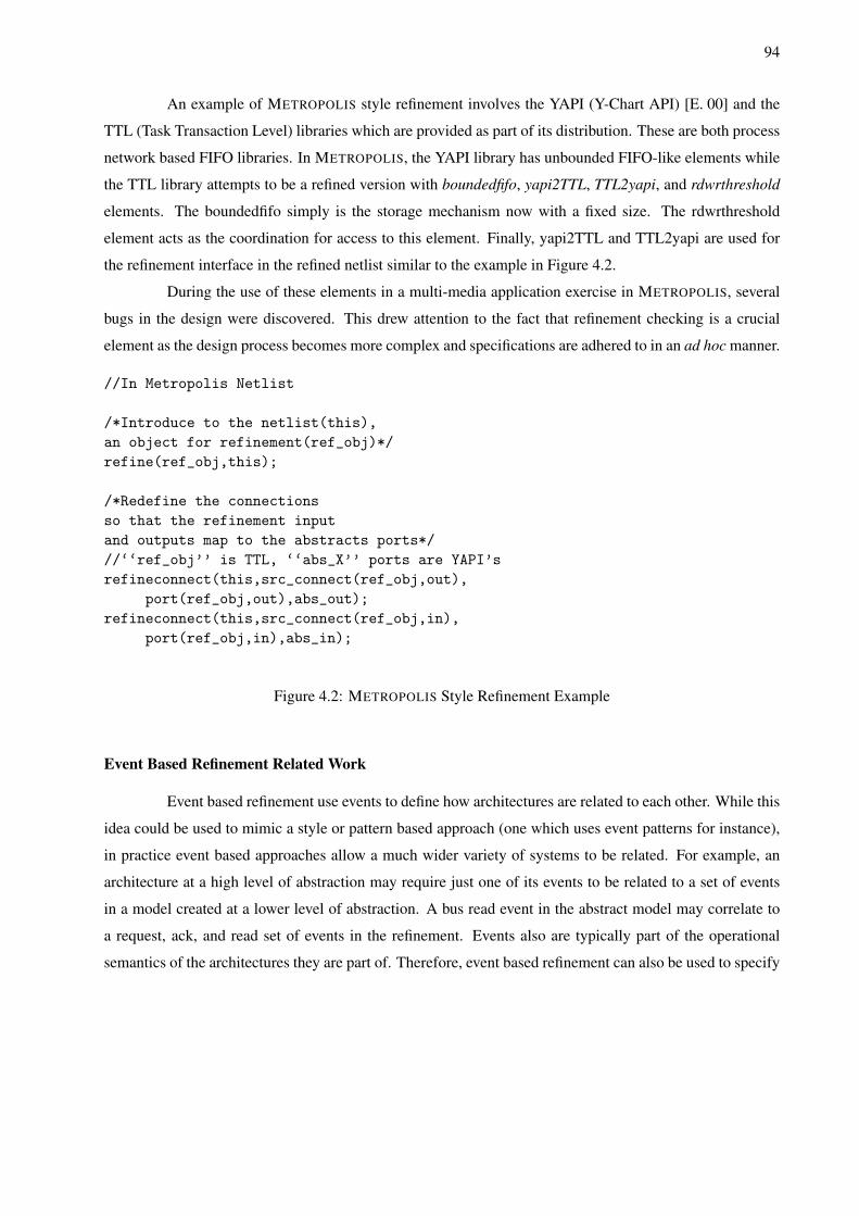
94
An example of METROPOLIS style refinement involves the YAPI (Y-Chart API) [E. 00] and the
TTL (Task Transaction Level) libraries which are provided as part of its distribution. These are both process
network based FIFO libraries. In METROPOLIS, the YAPI library has unbounded FIFO-like elements while
the TTL library attempts to be a refined version with boundedfifo, yapi2TTL, TTL2yapi, and rdwrthreshold
elements. The boundedfifo simply is the storage mechanism now with a fixed size. The rdwrthreshold
element acts as the coordination for access to this element. Finally, yapi2TTL and TTL2yapi are used for
the refinement interface in the refined netlist similar to the example in Figure 4.2.
During the use of these elements in a multi-media application exercise in METROPOLIS, several
bugs in the design were discovered. This drew attention to the fact that refinement checking is a crucial
element as the design process becomes more complex and specifications are adhered to in an ad hoc manner.
//In Metropolis Netlist
/*Introduce to the netlist(this),an object for refinement(ref_obj)*/refine(ref_obj,this);
/*Redefine the connectionsso that the refinement inputand outputs map to the abstracts ports*///‘‘ref_obj’’ is TTL, ‘‘abs_X’’ ports are YAPI’srefineconnect(this,src_connect(ref_obj,out),
port(ref_obj,out),abs_out);refineconnect(this,src_connect(ref_obj,in),
port(ref_obj,in),abs_in);
Figure 4.2: METROPOLIS Style Refinement Example
Event Based Refinement Related Work
Event based refinement use events to define how architectures are related to each other. While this
idea could be used to mimic a style or pattern based approach (one which uses event patterns for instance),
in practice event based approaches allow a much wider variety of systems to be related. For example, an
architecture at a high level of abstraction may require just one of its events to be related to a set of events
in a model created at a lower level of abstraction. A bus read event in the abstract model may correlate to
a request, ack, and read set of events in the refinement. Events also are typically part of the operational
semantics of the architectures they are part of. Therefore, event based refinement can also be used to specify
95
a specific operation or a restriction on system operation. For example a particular refinement may require the
notification of an event which triggers one behavior of many possible behaviors. The abstract model would
relax that notification requirement allowing more behaviors. An event based approach is shown in Rapide
[Dav95]. Rapide is an executable architecture definition language (EADL). Rapide uses “event patterns”
to relate architectures together during mapping. This should not be confused with patterns as previously
defined however, as Rapide uses these patterns or maps to trigger events or generate events. The event based
approach proposed in this work uses events to define properties. These properties could be seen as patterns
defined over a set of events. These properties use events specifically belonging to components depending on
their role in the simulation (either part of the scheduling or scheduled mechanism). This is different from
Rapide which does not make such a distinction. One can not directly make a comparison between the two
approaches outside of the fact that both require the notion of an event object defined as a tuple containing
more than one field of data.
Interface Based Refinement Related Work
Interface based refinement is premised on the fact that most modeling systems encapsulate services
through the use of interfaces. These interfaces often are a function of the language that the system is
described in. SystemC and Java for instance have the idea of interface functions for classes. Often times
however, the term interface denotes the legal interaction points between models and other models or models
and their environment. Refinement which focuses on these points is interface refinement. Typically changes
to the model which cannot be observed at the interface are not considered in this refinement style. Therefore
interface based refinement introduces a notion of observability not necessarily implied in the other styles.
The observability can be exploited in the event that a designer does not wish to have subsequent models be
viewed differently (e.g. keep the same interface) while at the same time this observability can be an issue
when design differences are desirable but difficult to push to the interfaces.
Interface based refinement methodologies are illustrated in the Reactive Modeling Language (RML)
[Raj99] and SPADE (System level Performance Analysis and Design space Exploration) [Pau01a]. In RML
a concept called hierarchical verification is employed. RML uses an object called a reactive model. These
reactive models can be composed to form composite objects. Hierarchical verification requires that every
finite sequence of observations resulting from the detailed module also be possible from the abstract model.
This work is directly relevant to the proposed methods in this chapter and will be discussed in more de-
tail. SPADE on the other hand uses Kahn Process Networks to describe functional models and a library
of architectural building blocks. The functional model creates traces. These traces can be “accepted” by

96
the architecture and contain information detailing which operation the architecture should perform. Trace
transformation is the process by which functionality is assigned to available architecture resources. This
transformation equates to forcing refinement traces to change to meet available architecture resources and
topologies. This style of work has also been used in Sesame [And06] which builds on the SPADE frame-
work. Refinement for these tools is a means to achieve a mapping. While mainly methodological in nature
the difference between this approach and a tool like METROPOLIS is that SPADE starts with a functional
description and works top down. METROPOLIS works both bottom up and top down, refining both architec-
tural services and functional descriptions independently.
Two other interface approaches are SynCo [Olg03b] and Signal [Jea03]. SynCo is based upon
the work of [Olg03a] which is a compositional component based methodology. Transitions systems for
both refined and abstraction systems are specified. States in those systems are then “glued” indicating which
states are required to correspond to each other (this is a many to one mapping from refined to abstract model).
Also synchronization mechanisms can be defined as well in order to create larger systems from individual
LTS. SynCo will be used in this thesis. Signal on the other hand is a polychronous (i.e. multiclocked)
design language. This language has the notion of flow equivalence between behaviors. This means that for
two behaviors their signals hold the same values for the same order. This leads to flow invariance where an
asynchronous implementation preserves flow equivalence.
Other approaches exist which can not be placed into one of the three previous classifications.
These often consist of ad hoc or brute strength style approaches. For example in [Nen96] the authors demon-
strate that object oriented (OO) subtype hierarchy type checking can be used to identify refinement. They
investigate how concepts in OO programming languages can be used in C2, a component and message based
system specification style. They find that by making subtyping explicit, identifying component substitution
is possible. Also extending type checking mechanisms allows a richer set of architectural relationships to
be expressed.
The proposed design flows in this thesis are a combination of event and interface based ap-
proaches. Specifically they most closely resemble the work of [Raj99] and [Olg03a] (both interface based).
For example they incorporate concepts such as trace containment, labeled transition systems or control
flow automata, and trace transformations. In fact the tools Mocha and SynCo are used in Chapter 5 on
several cases studies to actually implement the methodologies presented. This thesis could be extended
to style/pattern based approaches as well assuming a set of rules were created. Aspects of this process
were performed in early METROPOLIS related projects using both TTL and Yapi channels as proposed by
[Pau01b].
97
4.3 Event Based Service Refinement
Event based service refinement will be presented first. The presentation ordering was selected
because of the approaches presented here, event based is the most general. Events can be leveraged to
perform both interface and compositional component based verification as well (to be discussed). Event
oriented frameworks have become popular with the increased interest in exploring design frameworks which
allow specifying concurrent computation models. Lee and Sangiovanni in [Edw98] introduced the tagged
signal model which demonstrated how an event based framework can be used to express a variety of models
of computation. This characteristic has made them very flexible and gives them the ability to realize a wide
variety of systems. Also event based models are portable because often they only assume the presence of
events and do not make other assumptions about the framework which is implementing the events. Event
based platform refinement is prefaced upon the following ideas:
• The design framework uses events to denote system activity and provide synchronization mechanisms.
For example, imagine a basic producer and consumer example. The producer writes to a shared
storage location. Upon doing so, it produces an event (production) signaling this. It then waits for
the presence of another event (consumption). The consumer will use this notification (production) to
realize that it it can now consume the data. Upon consumption it will signal this operation with an
event (consumption) as well. This notifies the producer that it can safely produce again. This process
continues indefinitely.
• Sequences of events (traces) can be captured to recreate or represent system behavior. For example
a bus transaction has a fixed sequence of events as dictated by the protocol. A request event must
proceed a grant event for example. If this sequence is not maintained then the system behavior has
been violated.
• Event sequences can restrict or enforce behavior. For example often times a system has to make
choices. A control statement (if, while, for, etc) often has conditions which allow the system to make
a decision. Those conditions can use events as part of their evaluation. Allowing or restricting event
appearance can be an effective mechanism to enforce behavior without changing the model explicitly.
• This enforcement or restriction has the ability to be a well defined, methodological refinement as will
be shown in this thesis. Specifically examples will be shown in the METROPOLIS design environment
in Chapter 5.
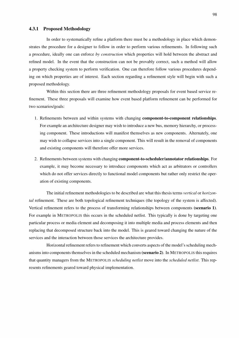
98
4.3.1 Proposed Methodology
In order to systematically refine a platform there must be a methodology in place which demon-
strates the procedure for a designer to follow in order to perform various refinements. In following such
a procedure, ideally one can enforce by construction which properties will hold between the abstract and
refined model. In the event that the construction can not be provably correct, such a method will allow
a property checking system to perform verification. One can therefore follow various procedures depend-
ing on which properties are of interest. Each section regarding a refinement style will begin with such a
proposed methodology.
Within this section there are three refinement methodology proposals for event based service re-
finement. These three proposals will examine how event based platform refinement can be performed for
two scenarios/goals:
1. Refinements between and within systems with changing component-to-component relationships.
For example an architecture designer may wish to introduce a new bus, memory hierarchy, or process-
ing component. These introductions will manifest themselves as new components. Alternately, one
may wish to collapse services into a single component. This will result in the removal of components
and existing components will therefore offer more services.
2. Refinements between systems with changing component-to-scheduler/annotator relationships. For
example, it may become necessary to introduce components which act as arbitrators or controllers
which do not offer services directly to functional model components but rather only restrict the oper-
ation of existing components.
The initial refinement methodologies to be described are what this thesis terms vertical or horizon-
tal refinement. These are both topological refinement techniques (the topology of the system is affected).
Vertical refinement refers to the process of transforming relationships between components (scenario 1).
For example in METROPOLIS this occurs in the scheduled netlist. This typically is done by targeting one
particular process or media element and decomposing it into multiple media and process elements and then
replacing that decomposed structure back into the model. This is geared toward changing the nature of the
services and the interaction between those services the architecture provides.
Horizontal refinement refers to refinement which converts aspects of the model’s scheduling mech-
anisms into components themselves in the scheduled mechanism (scenario 2). In METROPOLIS this requires
that quantity managers from the METROPOLIS scheduling netlist move into the scheduled netlist. This rep-
resents refinements geared toward physical implementation.
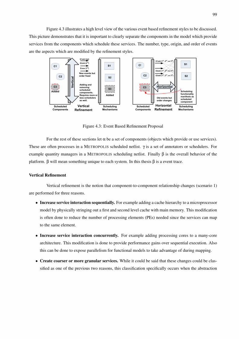
99
Figure 4.3 illustrates a high level view of the various event based refinement styles to be discussed.
This picture demonstrates that it is important to clearly separate the components in the model which provide
services from the components which schedule these services. The number, type, origin, and order of events
are the aspects which are modified by the refinement styles.
Scheduled
Components
Scheduling
Mechanisms
Scheduled
Components
Scheduling
Mechanisms
Scheduling
functionality
manifests as
scheduled
component
Adding and
removing
scheduled
components.
Requires more or
less schedulers
as well.
Vertical
Refinement
Horizontal
Refinement
E1old (1st)
E2old (2nd)
Enew (3rd)
E1old (1st, 2
nd, or 3
rd)
E2old (1st, 2
nd, or 3
rd)
E3old (1st, 2
nd, or 3
rd)
New events but
order fixed
Old events but
order changes
C1
C2
C3
C!
C2
S1
S2
S1
S2
S3C3
Added
Added
Vertical
Horizontal
Figure 4.3: Event Based Refinement Proposal
For the rest of these sections let α be a set of components (objects which provide or use services).
These are often processes in a METROPOLIS scheduled netlist. γ is a set of annotators or schedulers. For
example quantity managers in a METROPOLIS scheduling netlist. Finally β is the overall behavior of the
platform. β will mean something unique to each system. In this thesis β is a event trace.
Vertical Refinement
Vertical refinement is the notion that component-to-component relationship changes (scenario 1)
are performed for three reasons.
• Increase service interaction sequentially. For example adding a cache hierarchy to a microprocessor
model by physically stringing out a first and second level cache with main memory. This modification
is often done to reduce the number of processing elements (PEs) needed since the services can map
to the same element.
• Increase service interaction concurrently. For example adding processing cores to a many-core
architecture. This modification is done to provide performance gains over sequential execution. Also
this can be done to expose parallelism for functional models to take advantage of during mapping.
• Create coarser or more granular services. While it could be said that these changes could be clas-
sified as one of the previous two reasons, this classification specifically occurs when the abstraction
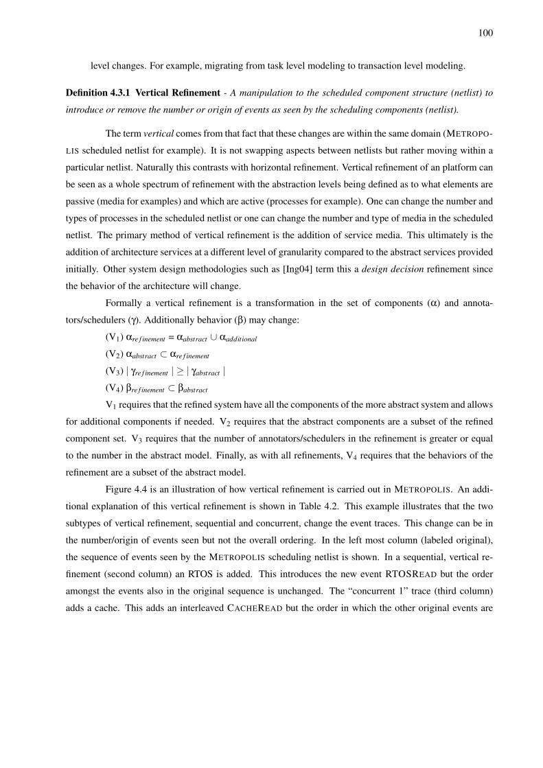
100
level changes. For example, migrating from task level modeling to transaction level modeling.
Definition 4.3.1 Vertical Refinement - A manipulation to the scheduled component structure (netlist) to
introduce or remove the number or origin of events as seen by the scheduling components (netlist).
The term vertical comes from that fact that these changes are within the same domain (METROPO-
LIS scheduled netlist for example). It is not swapping aspects between netlists but rather moving within a
particular netlist. Naturally this contrasts with horizontal refinement. Vertical refinement of an platform can
be seen as a whole spectrum of refinement with the abstraction levels being defined as to what elements are
passive (media for examples) and which are active (processes for example). One can change the number and
types of processes in the scheduled netlist or one can change the number and type of media in the scheduled
netlist. The primary method of vertical refinement is the addition of service media. This ultimately is the
addition of architecture services at a different level of granularity compared to the abstract services provided
initially. Other system design methodologies such as [Ing04] term this a design decision refinement since
the behavior of the architecture will change.
Formally a vertical refinement is a transformation in the set of components (α) and annota-
tors/schedulers (γ). Additionally behavior (β) may change:
(V1) αre f inement = αabstract ∪ αadditional
(V2) αabstract ⊂ αre f inement
(V3) | γre f inement | ≥ | γabstract |(V4) βre f inement ⊂ βabstract
V1 requires that the refined system have all the components of the more abstract system and allows
for additional components if needed. V2 requires that the abstract components are a subset of the refined
component set. V3 requires that the number of annotators/schedulers in the refinement is greater or equal
to the number in the abstract model. Finally, as with all refinements, V4 requires that the behaviors of the
refinement are a subset of the abstract model.
Figure 4.4 is an illustration of how vertical refinement is carried out in METROPOLIS. An addi-
tional explanation of this vertical refinement is shown in Table 4.2. This example illustrates that the two
subtypes of vertical refinement, sequential and concurrent, change the event traces. This change can be in
the number/origin of events seen but not the overall ordering. In the left most column (labeled original),
the sequence of events seen by the METROPOLIS scheduling netlist is shown. In a sequential, vertical re-
finement (second column) an RTOS is added. This introduces the new event RTOSREAD but the order
amongst the events also in the original sequence is unchanged. The “concurrent 1” trace (third column)
adds a cache. This adds an interleaved CACHEREAD but the order in which the other original events are
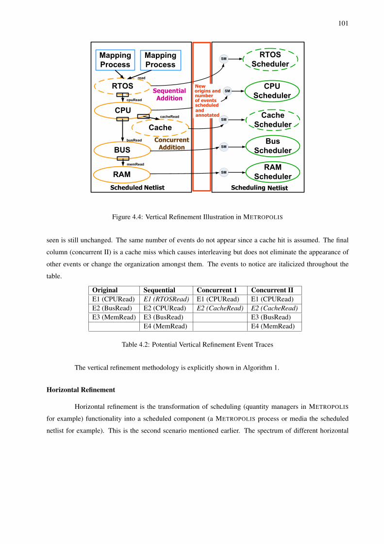
101
Neworigins andnumberof eventsscheduledand annotated
SM
SM
SM
SM
SM
memRead
busRead
cpuRead
cacheRead
read
Figure 4.4: Vertical Refinement Illustration in METROPOLIS
seen is still unchanged. The same number of events do not appear since a cache hit is assumed. The final
column (concurrent II) is a cache miss which causes interleaving but does not eliminate the appearance of
other events or change the organization amongst them. The events to notice are italicized throughout the
table.
Original Sequential Concurrent 1 Concurrent IIE1 (CPURead) E1 (RTOSRead) E1 (CPURead) E1 (CPURead)E2 (BusRead) E2 (CPURead) E2 (CacheRead) E2 (CacheRead)E3 (MemRead) E3 (BusRead) E3 (BusRead)
E4 (MemRead) E4 (MemRead)
Table 4.2: Potential Vertical Refinement Event Traces
The vertical refinement methodology is explicitly shown in Algorithm 1.
Horizontal Refinement
Horizontal refinement is the transformation of scheduling (quantity managers in METROPOLIS
for example) functionality into a scheduled component (a METROPOLIS process or media the scheduled
netlist for example). This is the second scenario mentioned earlier. The spectrum of different horizontal

102
Algorithm 1 Vertical Refinement Process1: Select service, S, to refine vertically {This decision is made based on DSE results and performance
desired}2: if S = MCSI or MCMI then
3: Add new component, CN
4: for all Components, Ci in S do
5: if Ci interacts with CN then
6: Add internal interfaces to Ci to accommodate, CN
7: end if
8: end for
9: else if S = SCSI then
10: Add new component, CN
11: Add one internal interface to accommodate, CN
12: Reclassify component as MCSI
13: else
14: Add new component, CN
15: Add quantity manager, QMNew {CN is a new stand alone component}16: Classify the component as SCSI
17: Register the service with the mapping process
18: end if
19: Reconnect the new topology
20: for all Events, E, between Netlistsched and Netlistscheduling do
21: Capture new behavior, BNew
22: end for
23: RETURN BNew
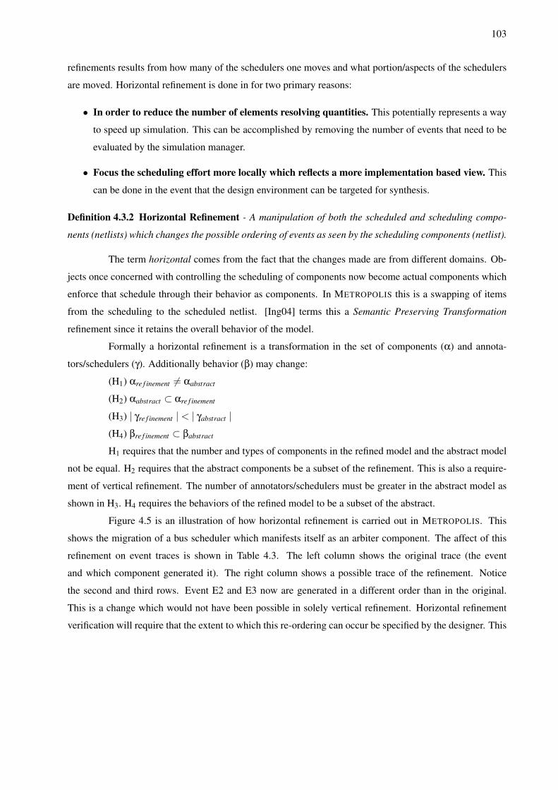
103
refinements results from how many of the schedulers one moves and what portion/aspects of the schedulers
are moved. Horizontal refinement is done in for two primary reasons:
• In order to reduce the number of elements resolving quantities. This potentially represents a way
to speed up simulation. This can be accomplished by removing the number of events that need to be
evaluated by the simulation manager.
• Focus the scheduling effort more locally which reflects a more implementation based view. This
can be done in the event that the design environment can be targeted for synthesis.
Definition 4.3.2 Horizontal Refinement - A manipulation of both the scheduled and scheduling compo-
nents (netlists) which changes the possible ordering of events as seen by the scheduling components (netlist).
The term horizontal comes from the fact that the changes made are from different domains. Ob-
jects once concerned with controlling the scheduling of components now become actual components which
enforce that schedule through their behavior as components. In METROPOLIS this is a swapping of items
from the scheduling to the scheduled netlist. [Ing04] terms this a Semantic Preserving Transformation
refinement since it retains the overall behavior of the model.
Formally a horizontal refinement is a transformation in the set of components (α) and annota-
tors/schedulers (γ). Additionally behavior (β) may change:
(H1) αre f inement 6= αabstract
(H2) αabstract ⊂ αre f inement
(H3) | γre f inement | < | γabstract |(H4) βre f inement ⊂ βabstract
H1 requires that the number and types of components in the refined model and the abstract model
not be equal. H2 requires that the abstract components be a subset of the refinement. This is also a require-
ment of vertical refinement. The number of annotators/schedulers must be greater in the abstract model as
shown in H3. H4 requires the behaviors of the refined model to be a subset of the abstract.
Figure 4.5 is an illustration of how horizontal refinement is carried out in METROPOLIS. This
shows the migration of a bus scheduler which manifests itself as an arbiter component. The affect of this
refinement on event traces is shown in Table 4.3. The left column shows the original trace (the event
and which component generated it). The right column shows a possible trace of the refinement. Notice
the second and third rows. Event E2 and E3 now are generated in a different order than in the original.
This is a change which would not have been possible in solely vertical refinement. Horizontal refinement
verification will require that the extent to which this re-ordering can occur be specified by the designer. This
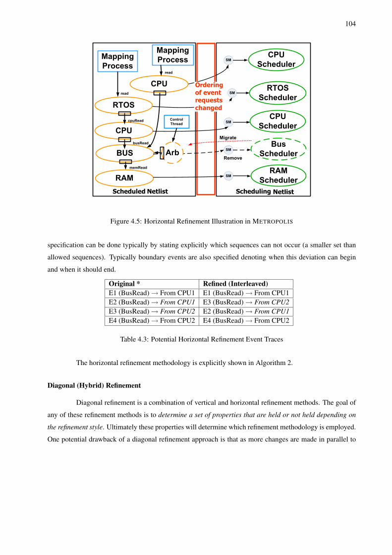
104
SM
SM
SM
SM
SM
memRead
busRead
cpuRead
read
read
Control
Thread
Remove
Migrate
Figure 4.5: Horizontal Refinement Illustration in METROPOLIS
specification can be done typically by stating explicitly which sequences can not occur (a smaller set than
allowed sequences). Typically boundary events are also specified denoting when this deviation can begin
and when it should end.
Original * Refined (Interleaved)E1 (BusRead) → From CPU1 E1 (BusRead) → From CPU1E2 (BusRead) → From CPU1 E3 (BusRead) → From CPU2E3 (BusRead) → From CPU2 E2 (BusRead) → From CPU1E4 (BusRead) → From CPU2 E4 (BusRead) → From CPU2
Table 4.3: Potential Horizontal Refinement Event Traces
The horizontal refinement methodology is explicitly shown in Algorithm 2.
Diagonal (Hybrid) Refinement
Diagonal refinement is a combination of vertical and horizontal refinement methods. The goal of
any of these refinement methods is to determine a set of properties that are held or not held depending on
the refinement style. Ultimately these properties will determine which refinement methodology is employed.
One potential drawback of a diagonal refinement approach is that as more changes are made in parallel to
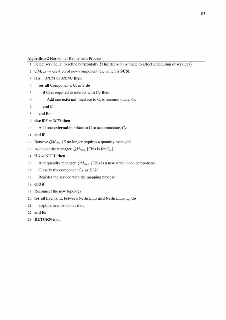
105
Algorithm 2 Horizontal Refinement Process1: Select service, S, to refine horizontally {This decision is made to affect scheduling of services}2: QMOld → creation of new component, CN which is SCSI
3: if S = MCSI or MCMI then
4: for all Components, Ci in S do
5: if Ci is required to interact with CN then
6: Add one external interface to Ci to accommodate, CN
7: end if
8: end for
9: else if S = SCSI then
10: Add one external interface to C to accommodate, CN
11: end if
12: Remove QMOld {S no longer requires a quantity manager}13: Add quantity manager, QMNew {This is for CN}14: if S = NULL then
15: Add quantity manager, QMNew {This is a new stand alone component}16: Classify the component CN as SCSI
17: Register the service with the mapping process
18: end if
19: Reconnect the new topology
20: for all Events, E, between Netlistsched and Netlistscheduling do
21: Capture new behavior, BNew
22: end for
23: RETURN BNew
106
a design, the more difficult (or impossible) it may become to determine the effects of the changes. The
methodological recommendation is that for any one refinement, each stage only consist of a vertical or
horizontal change followed by a verification of the relevant aspects before making any additional changes.
Event Based Properties
In order to make use of event based refinement methods, it is important to illustrate that properties
can be defined over events. These events will be of use in describing architectural services. The ability to
specify properties (event sequences) and verify these sequences is a key part of refinement. In Table 4.4 a
simple set of event traces demonstrates how to represent resource utilization. The table is first broken into
two sections. The left shows a “bad” resolve() function. The function resolve() is used in METROPOLIS
during the scheduling phase which enables events. The other side shows a “good” resolve(). In this case a
“good” resolve makes maximum use of the resources by scheduling events in such a way that resources are
not idle. For example assuming events E1, E2, and E3 only use the CPU whereas event E4 uses the CPU,
Bus, and Memory, it is ideal to let the Bus and Memory process the event E4 as soon as possible assuming
that the events are independent. In the “bad” resolve() scenario the events are scheduled E1, E2, E3, E4. The
P’s represent phases at which the elements are idle. The italicized Ps in the “bad” resolve() illustrate phases
in which resources are available but are not used. The difference can be seen in the “good” resolve which
schedules E4 first on the CPU thereby enabling this event to be seen earlier in the other components. This
property can be expressed later in such a way that allows the scheduling of events using the most resources
first in the event that events are independent.
Bad Resolve() Good Resolve ()CPU E1, E2, E3, E4 E4, E1, E2, E3Bus P4, P3, P2, P1, E4 P1, E4Mem P5, P4, P3, P2, P1, E4 P2, P1, E4
Table 4.4: Resource Utilization Event Analysis
In Table 4.5 the latency of two different simulations are shown. Again one side illustrates a “bad”
resolve() and the other side a “better” resolve(). Each resolve() side has two columns. The leftmost of
these columns shows the events to be scheduled. The rightmost of these columns shows the event selected.
In this case, “better” means that the average latency of events (time from generation to annotation of a
particular event) is minimized. Each element is labeled with a number in parenthesis which illustrates
which scheduling phase number is currently being evaluated. The italicized events illustrate key decision
points in the table. Starting with the “bad” resolve() side a description of the table is thus: initially the CPU
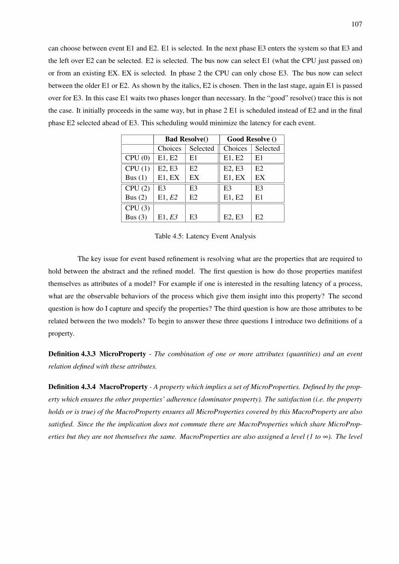
107
can choose between event E1 and E2. E1 is selected. In the next phase E3 enters the system so that E3 and
the left over E2 can be selected. E2 is selected. The bus now can select E1 (what the CPU just passed on)
or from an existing EX. EX is selected. In phase 2 the CPU can only chose E3. The bus now can select
between the older E1 or E2. As shown by the italics, E2 is chosen. Then in the last stage, again E1 is passed
over for E3. In this case E1 waits two phases longer than necessary. In the “good” resolve() trace this is not
the case. It initially proceeds in the same way, but in phase 2 E1 is scheduled instead of E2 and in the final
phase E2 selected ahead of E3. This scheduling would minimize the latency for each event.
Bad Resolve() Good Resolve ()Choices Selected Choices Selected
CPU (0) E1, E2 E1 E1, E2 E1CPU (1) E2, E3 E2 E2, E3 E2Bus (1) E1, EX EX E1, EX EXCPU (2) E3 E3 E3 E3Bus (2) E1, E2 E2 E1, E2 E1CPU (3)Bus (3) E1, E3 E3 E2, E3 E2
Table 4.5: Latency Event Analysis
The key issue for event based refinement is resolving what are the properties that are required to
hold between the abstract and the refined model. The first question is how do those properties manifest
themselves as attributes of a model? For example if one is interested in the resulting latency of a process,
what are the observable behaviors of the process which give them insight into this property? The second
question is how do I capture and specify the properties? The third question is how are those attributes to be
related between the two models? To begin to answer these three questions I introduce two definitions of a
property.
Definition 4.3.3 MicroProperty - The combination of one or more attributes (quantities) and an event
relation defined with these attributes.
Definition 4.3.4 MacroProperty - A property which implies a set of MicroProperties. Defined by the prop-
erty which ensures the other properties’ adherence (dominator property). The satisfaction (i.e. the property
holds or is true) of the MacroProperty ensures all MicroProperties covered by this MacroProperty are also
satisfied. Since the the implication does not commute there are MacroProperties which share MicroProp-
erties but they are not themselves the same. MacroProperties are also assigned a level (1 to ∞). The level

108
indicates the length of the longest chain of implications the MacroProperty is responsible for. MicroProper-
ties are by definition level 0.
Event Based Property Classification
This section will begin to discuss which properties can be specified during event based refinement.
Right now the list is very sparse and high level. The majority of effort will now go into identifying these
properties, their relationships, and how to check them.
One can categorize the properties as structural, functional, and performance. Platform-Based
design dictates that these be kept explicitly separate.
Examples of performance properties are:
• Latency - time for a task to complete. Given an appearance (start) time and a disappearance (end)
time of an event, the latency is the positive difference between the two.
• Throughput - number of tasks completed per unit time. Given a period of time (t) and a number of
completed tasks (TA), throughput is TA/t.
• CPI - cycles per instruction (request). This is simply an average to indicate system performance. For
example, the goal of a basic pipelined microprocessor is CPI=1. In the superscalar microprocessor
era, typically the inverse, IPC, is a more relevant metric.
• Jitter - random variation in a signal. For example given a periodic signal, the variation in the period
or amplitude is an example of jitter.
Performance properties typically have to do with specifications regarding the desire for a certain
level of performance. However sometimes these properties can actually be required for the correctness of a
system. This is often true of safety critical or real time systems. In many cases performance properties are
related to one another.
Examples of functional properties are:
• Mutex - mutual exclusion of a resource. This property can be realized by semaphores or shared
memory/variables. In many model languages such as SystemC events are used to accomplish this.
• Data Consistency/Coherence - global data set contents must match and reading and writing ordering
must be preserved. This property commonly is of interest in memory systems. Cache consistency and
coherency are often maintained by such protocols like MESI (Modified, Exclusive, Shared, Invalid).

109
Functional properties typically have to do with maintaining the correctness of a system. Often
they implicitly affect the performance properties of a system as well.
Examples of structural properties are:
• Memory Size - size of memory elements such as FIFOs. There exists both the physical memory as
well as the virtual memory. These can be distributed or shared memories.
• ALU operand size - the size of the ALU operands (i.e. bits). In addition to operand size, operation
type can also be important (floating point vs. integer).
• Datapath width - the size of the instruction and addressing datapaths. Datapath width may need to
change in the presence of instruction level parallelism such as VLIW machines or the adoption of a
new ISA.
Structural properties typically have to do with both the performance and the correctness of a
system. They will interact with other structural properties as well as with functional and performance
properties.
What will be of key importance is the way in which properties are related and categorized so that
one can:
• Determine which properties are related and how. This can be defined over sets of Micro and Macro
properties.
• Determine which refinements relate to which properties. These can be defined both explicitly (i.e. a
list of required properties), construction (i.e. certain refinements automatically preserve properties),
or implicitly (i.e. one property preservation requires the adherence of another).
In terms of grouping properties an initial attempt I have seen is in [Rat98] which describes a
method which uses the following terminology:
• Rule of Computation (CMP) - dictates how variable (stored) values are computed based on their old
values as well other variables.
• Rule of Read Order (RO) - for any pair of read events x and y in a process, if x comes before y in
program order, then x occurs before y.
• Rule of Write Order (WO) - for any pair of write events a and b in a process, if a comes before b in
program order, then a occurs before b.

110
• Rule of Write Atomicity (WA) - writes become instantly visible to all processes instantaneously.
One can group properties by this method. For example the “mutex” functional property is a WA
property. While Data consistency is a RO and WO property. This method can be used to examine Macro
and Micro properties relationships.
Event Based Property Relationships
This section will describe how property relationships can be established. This is a key to the Micro
and Macro properties discussed earlier. These relationships will be needed to check event based refinement
in an efficient manner both in terms of its specification as well is its execution time. Here are several
examples indicating the relationship and hierarchy of Micro and Macro properties. Future work outside of
this thesis will be devoted to establishing these relationships more formally.
1. Data Consistency → Sufficient Space, Read Access, Write Access
In the case of this relationship, if the MacroProperty “Data Consistency” (DC) is proven, it then
implies the MicroProperties “Sufficient Space” (SS), “Read Access” (RA), and “Write Access” (WA).
SS indicates that the data storage device itself has enough space. RA indicates that the storage device
is allowing reads. WA indicates that the storage device is allowing writes. Notice that proving the
MicroProperties SS, RA, or WA does not imply anything else at this point. However, assume that WA
and RA were transformed into a MacroProperties such that:
• Write Access → SS
• Read Access → Data Valid
In this case, SS is the same MicroProperty as described previously and “Data Valid” (DV) indicates
that the data is marked as being valid in the storage device (i.e. during a cache or snooping update).
If these MacroProperties are proposed and proven, then “Data Consistency” actually implies DV as
well in addition to the other MicroProperties mentioned previously. It also will imply SS transitively
through MacroProperty hierarchies and would not have to imply it explicitly. “Data Consistency” is
a RO and WO property in terms of its grouping as well as a performance property in terms of its
classification.
2. Data Coherency → Data Valid, Snoop Complete
Notice that “Data Coherency” (DCo) implies DV. RA implies this MicroProperty as well and RA is
implied by DC. However simply because DCo and RA share a MicroProperty they do not imply each
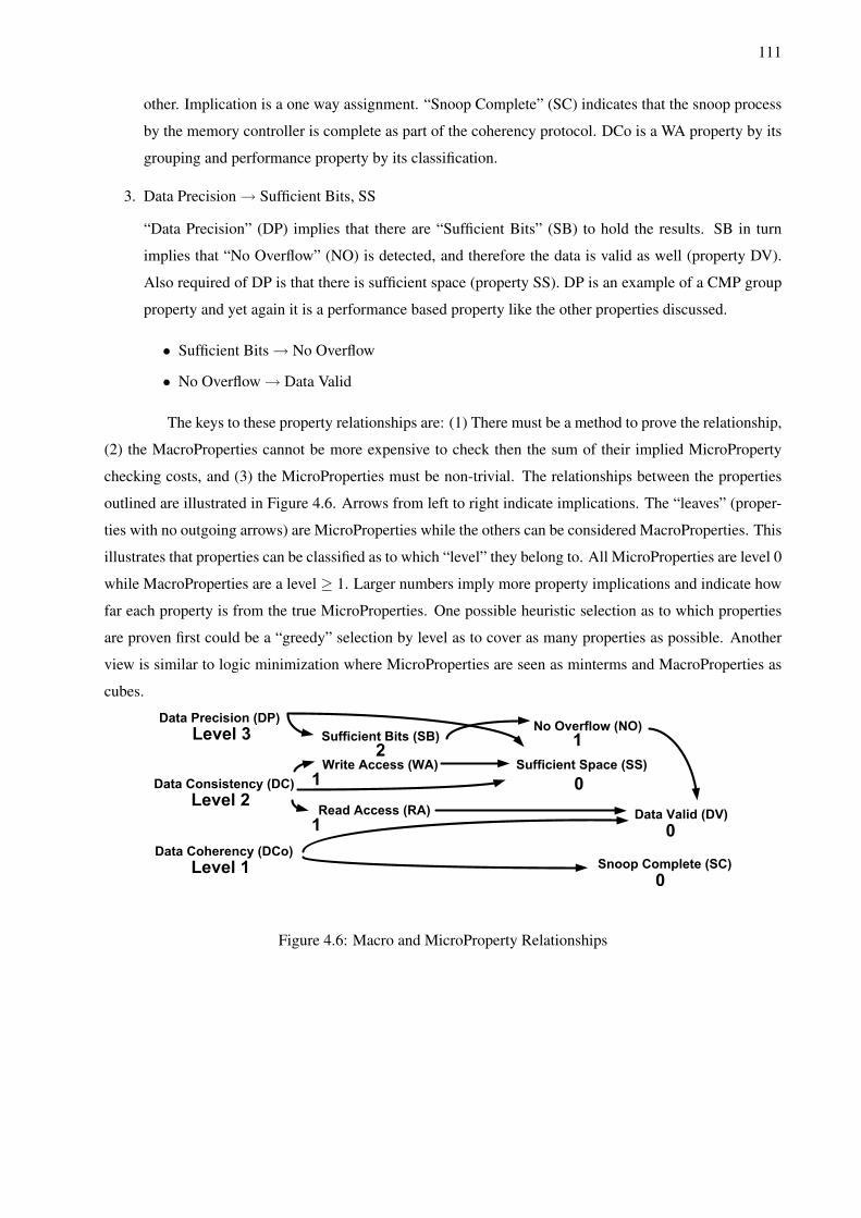
111
other. Implication is a one way assignment. “Snoop Complete” (SC) indicates that the snoop process
by the memory controller is complete as part of the coherency protocol. DCo is a WA property by its
grouping and performance property by its classification.
3. Data Precision → Sufficient Bits, SS
“Data Precision” (DP) implies that there are “Sufficient Bits” (SB) to hold the results. SB in turn
implies that “No Overflow” (NO) is detected, and therefore the data is valid as well (property DV).
Also required of DP is that there is sufficient space (property SS). DP is an example of a CMP group
property and yet again it is a performance based property like the other properties discussed.
• Sufficient Bits → No Overflow
• No Overflow → Data Valid
The keys to these property relationships are: (1) There must be a method to prove the relationship,
(2) the MacroProperties cannot be more expensive to check then the sum of their implied MicroProperty
checking costs, and (3) the MicroProperties must be non-trivial. The relationships between the properties
outlined are illustrated in Figure 4.6. Arrows from left to right indicate implications. The “leaves” (proper-
ties with no outgoing arrows) are MicroProperties while the others can be considered MacroProperties. This
illustrates that properties can be classified as to which “level” they belong to. All MicroProperties are level 0
while MacroProperties are a level ≥ 1. Larger numbers imply more property implications and indicate how
far each property is from the true MicroProperties. One possible heuristic selection as to which properties
are proven first could be a “greedy” selection by level as to cover as many properties as possible. Another
view is similar to logic minimization where MicroProperties are seen as minterms and MacroProperties as
cubes.
Data Consistency (DC)
Data Coherency (DCo)
Write Access (WA)
Read Access (RA)
Sufficient Space (SS)
Data Valid (DV)
Sufficient Bits (SB)No Overflow (NO)
Snoop Complete (SC)
Data Precision (DP)
Figure 4.6: Macro and MicroProperty Relationships
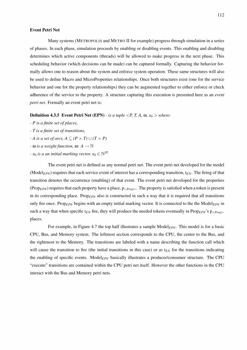
112
Event Petri Net
Many systems (METROPOLIS and METRO II for example) progress through simulation in a series
of phases. In each phase, simulation proceeds by enabling or disabling events. This enabling and disabling
determines which active components (threads) will be allowed to make progress in the next phase. This
scheduling behavior (which decisions can be made) can be captured formally. Capturing the behavior for-
mally allows one to reason about the system and enforce system operation. These same structures will also
be used to define Macro and MicroProperties relationships. Once both structures exist (one for the service
behavior and one for the property relationships) they can be augmented together to either enforce or check
adherence of the service to the property. A structure capturing this execution is presented here as an event
petri net. Formally an event petri net is:
Definition 4.3.5 Event Petri Net (EPN) - is a tuple <P, T, A, ω, x0 > where:
- P is a finite set of places,
- T is a finite set of transitions,
- A is a set of arcs, A ⊆ (P × T) ∪ (T × P)
- ω is a weight function, ω: A → N
- x0 is a an initial marking vector, x0 ∈ N|P|
The event petri net is defined as any normal petri net. The event petri net developed for the model
(ModelEPN) requires that each service event of interest has a corresponding transition, tEN . The firing of that
transition denotes the occurrence (enabling) of that event. The event petri net developed for the properties
(PropEPN) requires that each property have a place, p<Prop>. The property is satisfied when a token is present
in its corresponding place. PropEPN also is constructed in such a way that it is required that all transitions
only fire once. PropEPN begins with an empty initial marking vector. It is connected to the the ModelEPN in
such a way that when specific tEN fire, they will produce the needed tokens eventually in PropEPN’s p<Prop>
places.
For example, in Figure 4.7 the top half illustrates a sample ModelEPN . This model is for a basic
CPU, Bus, and Memory system. The leftmost section corresponds to the CPU, the center to the Bus, and
the rightmost to the Memory. The transitions are labeled with a name describing the function call which
will cause the transition to fire (the initial transitions in this case) or as tEN for the transitions indicating
the enabling of specific events. ModelEPN basically illustrates a producer/consumer structure. The CPU
“execute” transitions are contained within the CPU petri net itself. However the other functions in the CPU
interact with the Bus and Memory petri nets.
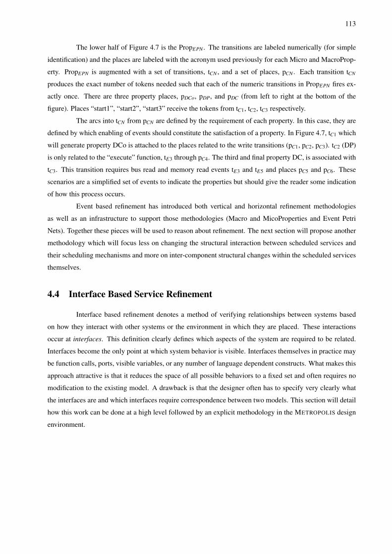
113
The lower half of Figure 4.7 is the PropEPN . The transitions are labeled numerically (for simple
identification) and the places are labeled with the acronym used previously for each Micro and MacroProp-
erty. PropEPN is augmented with a set of transitions, tCN , and a set of places, pCN . Each transition tCN
produces the exact number of tokens needed such that each of the numeric transitions in PropEPN fires ex-
actly once. There are three property places, pDCo, pDP, and pDC (from left to right at the bottom of the
figure). Places “start1”, “start2”, “start3” receive the tokens from tC1, tC2, tC3 respectively.
The arcs into tCN from pCN are defined by the requirement of each property. In this case, they are
defined by which enabling of events should constitute the satisfaction of a property. In Figure 4.7, tC1 which
will generate property DCo is attached to the places related to the write transitions (pC1, pC2, pC3). tC2 (DP)
is only related to the “execute” function, tE3 through pC4. The third and final property DC, is associated with
tC3. This transition requires bus read and memory read events tE3 and tE5 and places pC5 and pC6. These
scenarios are a simplified set of events to indicate the properties but should give the reader some indication
of how this process occurs.
Event based refinement has introduced both vertical and horizontal refinement methodologies
as well as an infrastructure to support those methodologies (Macro and MicoProperties and Event Petri
Nets). Together these pieces will be used to reason about refinement. The next section will propose another
methodology which will focus less on changing the structural interaction between scheduled services and
their scheduling mechanisms and more on inter-component structural changes within the scheduled services
themselves.
4.4 Interface Based Service Refinement
Interface based refinement denotes a method of verifying relationships between systems based
on how they interact with other systems or the environment in which they are placed. These interactions
occur at interfaces. This definition clearly defines which aspects of the system are required to be related.
Interfaces become the only point at which system behavior is visible. Interfaces themselves in practice may
be function calls, ports, visible variables, or any number of language dependent constructs. What makes this
approach attractive is that it reduces the space of all possible behaviors to a fixed set and often requires no
modification to the existing model. A drawback is that the designer often has to specify very clearly what
the interfaces are and which interfaces require correspondence between two models. This section will detail
how this work can be done at a high level followed by an explicit methodology in the METROPOLIS design
environment.
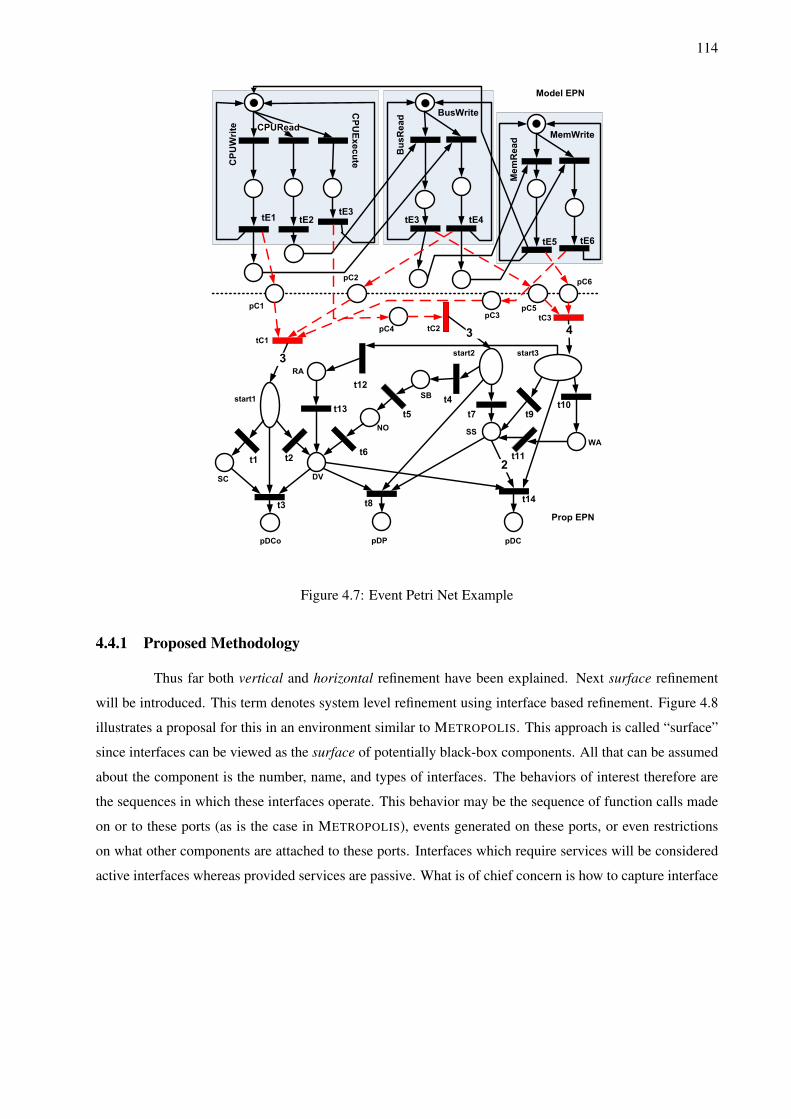
114
DVSC
pDCo
t1 t2
t3
NO
SB
SS
pDP
RA
WA
2
pDC
t4
t5
t6
t7
t8
t9t10
t11
t12
t13
t14
3
3 4
BusRead
BusWrite
CPUWrite
CPUExecute
MemRead
MemWriteCPURead
tE1 tE2tE3
tE3 tE4
tE5 tE6
tC1
tC2
tC3
pC1
pC2
pC4
pC3pC5
pC6
start1
start2 start3
Model EPN
Prop EPN
Figure 4.7: Event Petri Net Example
4.4.1 Proposed Methodology
Thus far both vertical and horizontal refinement have been explained. Next surface refinement
will be introduced. This term denotes system level refinement using interface based refinement. Figure 4.8
illustrates a proposal for this in an environment similar to METROPOLIS. This approach is called “surface”
since interfaces can be viewed as the surface of potentially black-box components. All that can be assumed
about the component is the number, name, and types of interfaces. The behaviors of interest therefore are
the sequences in which these interfaces operate. This behavior may be the sequence of function calls made
on or to these ports (as is the case in METROPOLIS), events generated on these ports, or even restrictions
on what other components are attached to these ports. Interfaces which require services will be considered
active interfaces whereas provided services are passive. What is of chief concern is how to capture interface
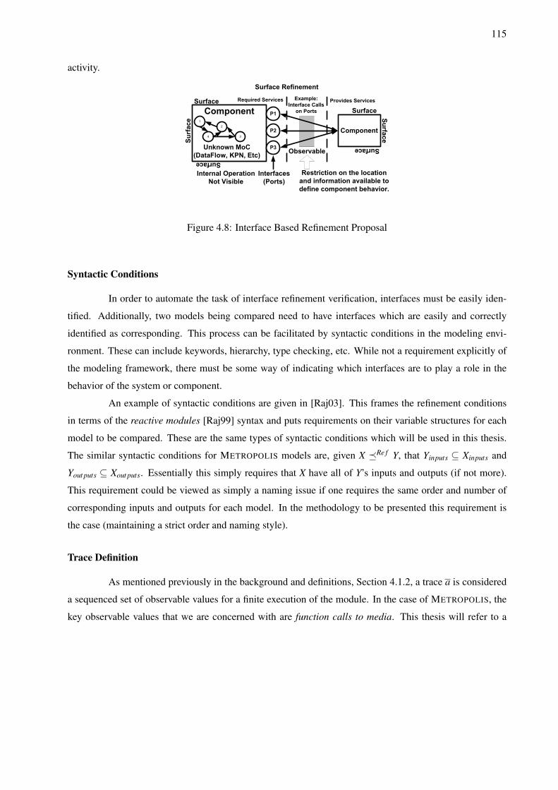
115
activity.
P1
P3
P2
1
3
2
4
Interfaces
(Ports)
Internal Operation
Not Visible
Example:
Interface Calls
on Ports
Unknown MoC
(DataFlow, KPN, Etc)Observable
Provides Services
Component
Surface
Surface
Surface
Required Services
Surface Refinement
Restriction on the location
and information available to
define component behavior.
Surface
Surface
Surface
Figure 4.8: Interface Based Refinement Proposal
Syntactic Conditions
In order to automate the task of interface refinement verification, interfaces must be easily iden-
tified. Additionally, two models being compared need to have interfaces which are easily and correctly
identified as corresponding. This process can be facilitated by syntactic conditions in the modeling envi-
ronment. These can include keywords, hierarchy, type checking, etc. While not a requirement explicitly of
the modeling framework, there must be some way of indicating which interfaces are to play a role in the
behavior of the system or component.
An example of syntactic conditions are given in [Raj03]. This frames the refinement conditions
in terms of the reactive modules [Raj99] syntax and puts requirements on their variable structures for each
model to be compared. These are the same types of syntactic conditions which will be used in this thesis.
The similar syntactic conditions for METROPOLIS models are, given X �Re f Y, that Yinputs ⊆ Xinputs and
Yout puts ⊆ Xout puts. Essentially this simply requires that X have all of Y’s inputs and outputs (if not more).
This requirement could be viewed as simply a naming issue if one requires the same order and number of
corresponding inputs and outputs for each model. In the methodology to be presented this requirement is
the case (maintaining a strict order and naming style).
Trace Definition
As mentioned previously in the background and definitions, Section 4.1.2, a trace a is considered
a sequenced set of observable values for a finite execution of the module. In the case of METROPOLIS, the
key observable values that we are concerned with are function calls to media. This thesis will refer to a
116
trace consisting of function calls to media as a TraceM, where the “M” stands for “Metropolis”. Due to the
semantics of METROPOLIS, processes must communicate strictly via media. This restriction could exist in
METRO II as well but since media are not present in this environment, it would be component-to-component
connections. Ultimately the behavior of a process/component can be characterized by the sequence by which
it makes these calls. Syntactically this results in an interface call attached to a particular port.
Definition 4.4.1 METROPOLIS Interface Behavior - a sequenced set of observable values for a finite
execution of the model, TraceM. This sequence results from function calls on ports requesting (requiring)
services.
In order to characterize the METROPOLIS TRACE, TraceM, the key structure needed to be obtained
from the model is the control flow automata (CFA) concerning the ways in which these sets of observable
events can occur. Once this structure is created State Equivalence concepts such as Bisimilarity and Simi-
larity [Raj03] can be used to determine refinement. A TraceM can be obtained by traversing this structure.
This structure is described in Section 4.4.1. Before describing this structure however, one must select which
set of interfaces should be considered for this structure. These sets are defined by what this thesis calls,
refinement domains.
Refinement Domains
Naturally in a design there are many interfaces. However during refinement it may not be neces-
sary or appropriate to consider all of these interfaces during refinement verification. Often components are
composed in such a way that there is a single set of interfaces which capture the behavior sufficiently of the
set of the components. These collections of components are termed, refinement domains, specifically:
Definition 4.4.2 Refinement Domain - a collection of components C, ports P, and observed ports OP.
Typically organized by component service. <C, P, OP> where OP ⊆ P.
The refinement domain definition illustrates that only a subset of ports are involved in the inter-
faces to be verified. The components are typically organized into domains such as computation, communi-
cation, and storage. These organizations are constructed in such a way to minimize the number of observed
ports needed.
Computation domains collect components involved in computation such as adders, multipliers,
processing elements, etc. Interfaces typically have to do with the execution of specific services. An example
of a refinement domain specifying interactions of interest in computation is when one changes from using
117
an adder to multiply values to a dedicated multiplier. All that matters is the input and output interfaces, not
the interfaces between the various adder or multiplier blocks.
Communication domains contain components such as buses, bridges, switch fabric, and buffers.
Interfaces have to do with reading, writing, synchronization, or data movement. For example, two buses
may be connected with a bridge. The interaction of interest is not between the buses and the bridge but
rather that the end to end behavior is maintained. Hence bridge interfaces may be ignored.
Finally storage domains contain main memory, cache, or scratch pad storage. Interfaces have to
do with loading and storing. Often with memory hierarchy one may add a new component (i.e. a cache).
One is not interested in the cache’s relationship with main memory but rather with the boundary between
the memory system and the components which need the data stored there. One can restrict refinement only
to those interfaces.
An example of refinement domains is clearly illustrated in Figure 4.9. This is an example based on
a FLEET style dataflow system. The left hand side shows the original system. This system consists of two
computation refinement domains (Adder and Producer based) and one communication refinement domain
(Switch Fabric based). One unique component is assigned to each of the three domains. One can see which
function calls each component can make next to the component itself. These include, “move.source.Adder”,
“prodLit()”, and “Add(input1, input2)” for example. What is illustrated is a potential graph showing function
interaction in each system. A graph is composed of locations and arcs. The locations are states of the system
as it proceeds through its execution. The transitions occur as function calls are made in each refinement
domain. In the original system, the adder has two states. The first state waits for data. When data arrives, it
can perform the addition and transition to the next state. The adder can then move the result to the switch
fabric. The switch fabric can move the data back into the adder through a series of move instructions. The
producer on the other hand waits to produce a literal value. Once this occurs, it transitions to its second
state. From this state the produced literal can be passed through the switch fabric to the adder or back into
the producer and used as a seed to produce another literal.
On the right hand side of the figure, the second system is shown. In this case a memory component
is added to the system. This is an newly introduced storage refinement domain. Also a new computation
domain is defined combining both the adder and the producer. These additions can be seen as refinements.
Restrictions have been made regarding the source and destination behavior as well. For example, the pro-
ducer can only be addressed through the adder now. The computation refinement domain now waits to
“add” and then proceeds to the next state after the “Add(input1, input2)” function execution. This system
now will transition to a state in which a literal value based on the addition operation is produced through
the “prodLit()” function. The switch fabric now can route data to the memory component, or to the states
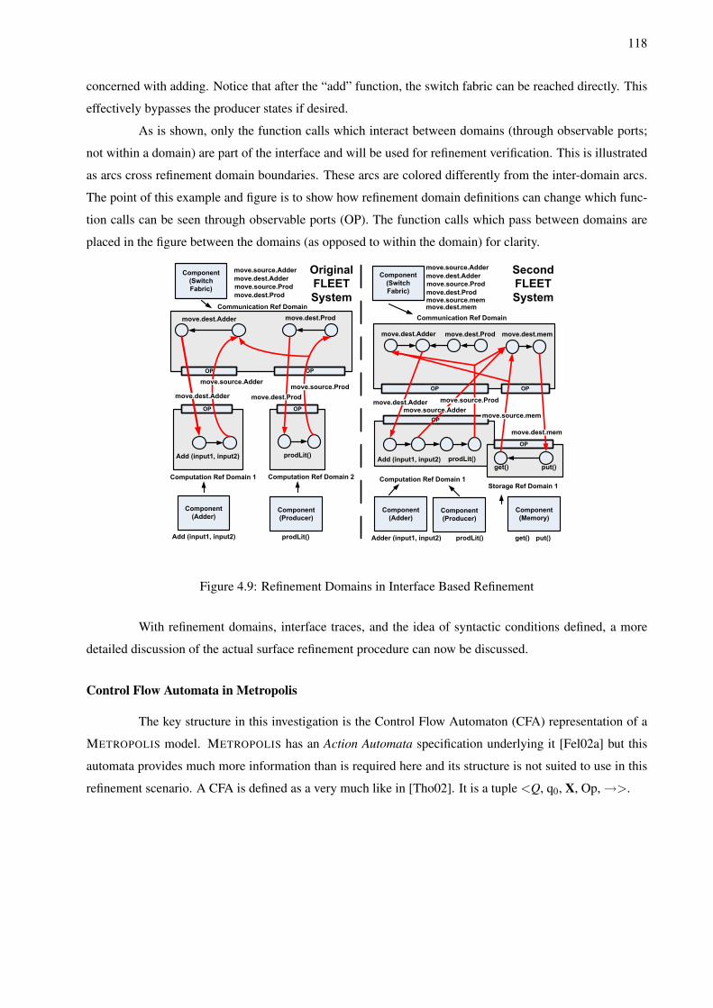
118
concerned with adding. Notice that after the “add” function, the switch fabric can be reached directly. This
effectively bypasses the producer states if desired.
As is shown, only the function calls which interact between domains (through observable ports;
not within a domain) are part of the interface and will be used for refinement verification. This is illustrated
as arcs cross refinement domain boundaries. These arcs are colored differently from the inter-domain arcs.
The point of this example and figure is to show how refinement domain definitions can change which func-
tion calls can be seen through observable ports (OP). The function calls which pass between domains are
placed in the figure between the domains (as opposed to within the domain) for clarity.
Component
(Producer)
Component
(Adder)Component
(Producer)
Component
(Adder)
Component
(Memory)
move.source.Prod
move.dest.Prod
move.source.Adder
move.dest.Adder
move.source.memmove.dest.mem
Component
(Switch
Fabric)
Component
(Switch
Fabric)
Add (input1, input2) Adder (input1, input2)prodLit() prodLit() get() put()
move.dest.Adder move.dest.Prod
Add (input1, input2) prodLit()
move.dest.Adder move.dest.Prod move.dest.mem
prodLit()Add (input1, input2)get() put()
Communication Ref Domain
Computation Ref Domain 1 Computation Ref Domain 2 Computation Ref Domain 1
Communication Ref Domain
Storage Ref Domain 1
OP OP
OPOP
OP
OP
OP OP
move.source.Prod
move.dest.Prod
move.source.Adder
move.dest.Adder
move.source.Adder
move.dest.Adder move.dest.Prod
move.source.Prod
move.source.mem
move.dest.mem
move.source.Adder
move.source.Prodmove.dest.Adder
Figure 4.9: Refinement Domains in Interface Based Refinement
With refinement domains, interface traces, and the idea of syntactic conditions defined, a more
detailed discussion of the actual surface refinement procedure can now be discussed.
Control Flow Automata in Metropolis
The key structure in this investigation is the Control Flow Automaton (CFA) representation of a
METROPOLIS model. METROPOLIS has an Action Automata specification underlying it [Fel02a] but this
automata provides much more information than is required here and its structure is not suited to use in this
refinement scenario. A CFA is defined as a very much like in [Tho02]. It is a tuple <Q, q0, X, Op, →>.
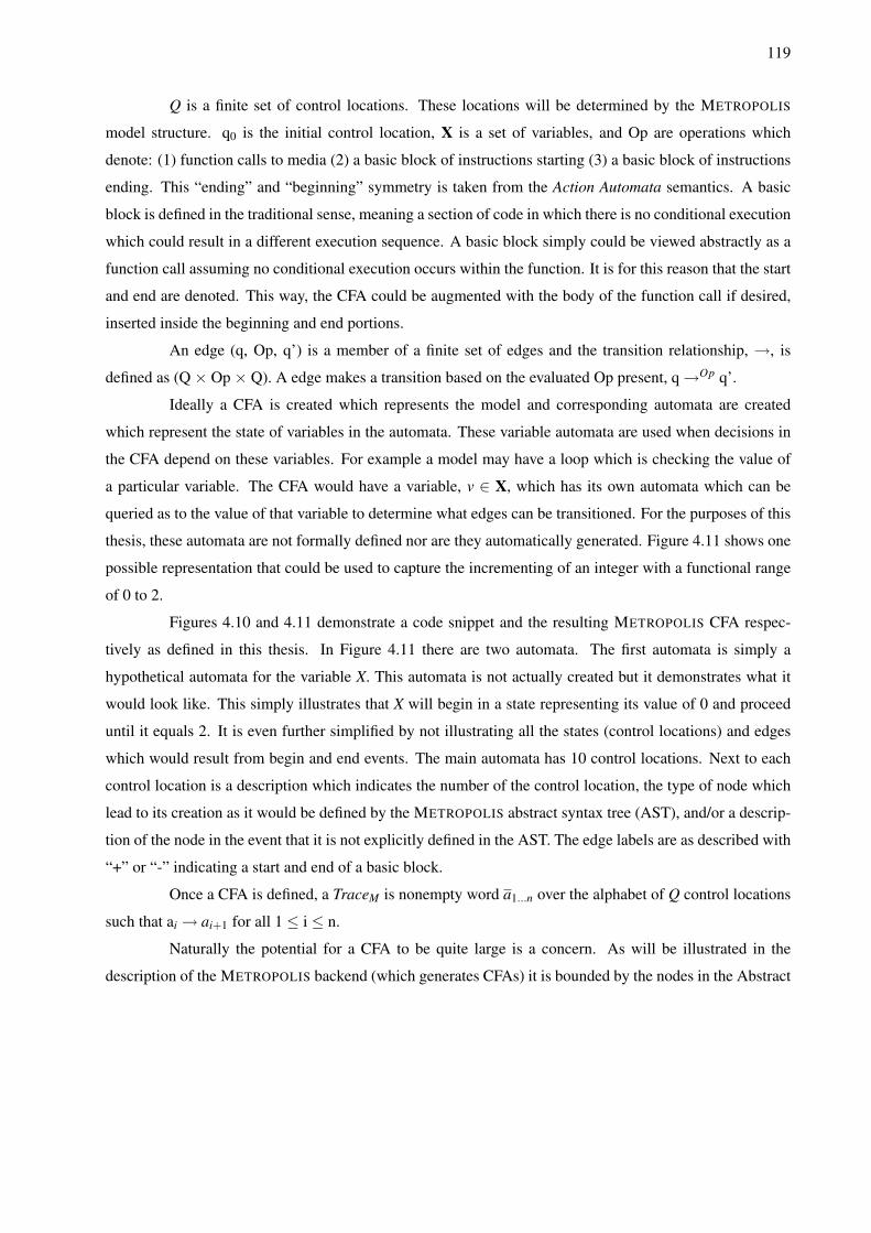
119
Q is a finite set of control locations. These locations will be determined by the METROPOLIS
model structure. q0 is the initial control location, X is a set of variables, and Op are operations which
denote: (1) function calls to media (2) a basic block of instructions starting (3) a basic block of instructions
ending. This “ending” and “beginning” symmetry is taken from the Action Automata semantics. A basic
block is defined in the traditional sense, meaning a section of code in which there is no conditional execution
which could result in a different execution sequence. A basic block simply could be viewed abstractly as a
function call assuming no conditional execution occurs within the function. It is for this reason that the start
and end are denoted. This way, the CFA could be augmented with the body of the function call if desired,
inserted inside the beginning and end portions.
An edge (q, Op, q’) is a member of a finite set of edges and the transition relationship, →, is
defined as (Q × Op × Q). A edge makes a transition based on the evaluated Op present, q →Op q’.
Ideally a CFA is created which represents the model and corresponding automata are created
which represent the state of variables in the automata. These variable automata are used when decisions in
the CFA depend on these variables. For example a model may have a loop which is checking the value of
a particular variable. The CFA would have a variable, v ∈ X, which has its own automata which can be
queried as to the value of that variable to determine what edges can be transitioned. For the purposes of this
thesis, these automata are not formally defined nor are they automatically generated. Figure 4.11 shows one
possible representation that could be used to capture the incrementing of an integer with a functional range
of 0 to 2.
Figures 4.10 and 4.11 demonstrate a code snippet and the resulting METROPOLIS CFA respec-
tively as defined in this thesis. In Figure 4.11 there are two automata. The first automata is simply a
hypothetical automata for the variable X. This automata is not actually created but it demonstrates what it
would look like. This simply illustrates that X will begin in a state representing its value of 0 and proceed
until it equals 2. It is even further simplified by not illustrating all the states (control locations) and edges
which would result from begin and end events. The main automata has 10 control locations. Next to each
control location is a description which indicates the number of the control location, the type of node which
lead to its creation as it would be defined by the METROPOLIS abstract syntax tree (AST), and/or a descrip-
tion of the node in the event that it is not explicitly defined in the AST. The edge labels are as described with
“+” or “-” indicating a start and end of a basic block.
Once a CFA is defined, a TraceM is nonempty word a1...n over the alphabet of Q control locations
such that ai → ai+1 for all 1 ≤ i ≤ n.
Naturally the potential for a CFA to be quite large is a concern. As will be illustrated in the
description of the METROPOLIS backend (which generates CFAs) it is bounded by the nodes in the Abstract
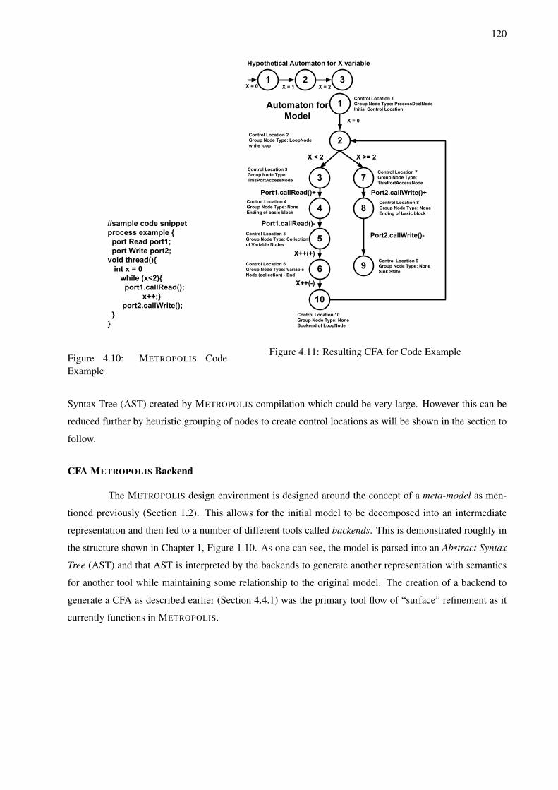
120
//sample code snippet
process example {
port Read port1;
port Write port2;
void thread(){
int x = 0
while (x<2){
port1.callRead();
x++;}
port2.callWrite();
}
}
Figure 4.10: METROPOLIS CodeExample
Control Location 1
Group Node Type: ProcessDeclNode
Initial Control Location
X = 0
Control Location 2
Group Node Type: LoopNode
while loop
X < 2 X >= 2
Control Location 7
Group Node Type:
ThisPortAccessNode
Control Location 8
Group Node Type: None
Ending of basic block
Port2.callWrite()+
Port2.callWrite()-
Control Location 9
Group Node Type: None
Sink State
Control Location 10
Group Node Type: None
Bookend of LoopNode
Port1.callRead()+
Port1.callRead()-
X++(+)
X++(-)
Control Location 3
Group Node Type:
ThisPortAccessNode
Control Location 4
Group Node Type: None
Ending of basic block
Control Location 5
Group Node Type: Collection
of Variable Nodes
Control Location 6
Group Node Type: Variable
Node (collection) - End
X = 0 X = 1 X = 2
Hypothetical Automaton for X variable
Figure 4.11: Resulting CFA for Code Example
Syntax Tree (AST) created by METROPOLIS compilation which could be very large. However this can be
reduced further by heuristic grouping of nodes to create control locations as will be shown in the section to
follow.
CFA METROPOLIS Backend
The METROPOLIS design environment is designed around the concept of a meta-model as men-
tioned previously (Section 1.2). This allows for the initial model to be decomposed into an intermediate
representation and then fed to a number of different tools called backends. This is demonstrated roughly in
the structure shown in Chapter 1, Figure 1.10. As one can see, the model is parsed into an Abstract Syntax
Tree (AST) and that AST is interpreted by the backends to generate another representation with semantics
for another tool while maintaining some relationship to the original model. The creation of a backend to
generate a CFA as described earlier (Section 4.4.1) was the primary tool flow of “surface” refinement as it
currently functions in METROPOLIS.
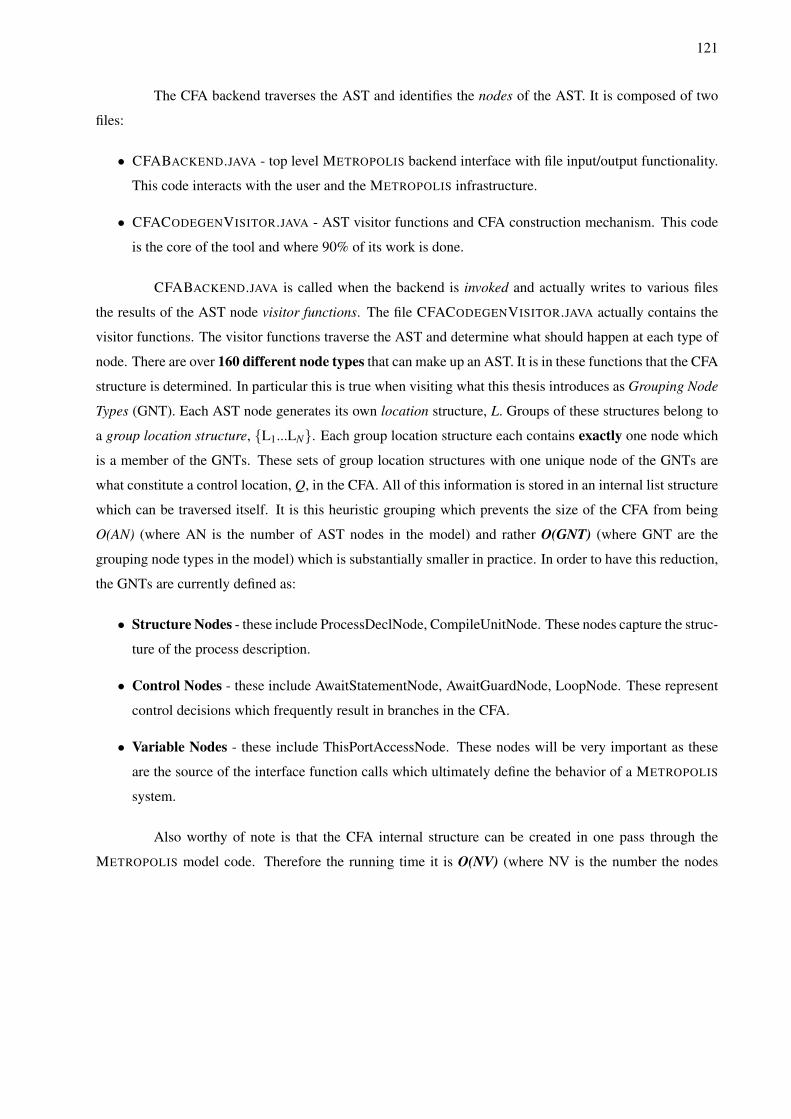
121
The CFA backend traverses the AST and identifies the nodes of the AST. It is composed of two
files:
• CFABACKEND.JAVA - top level METROPOLIS backend interface with file input/output functionality.
This code interacts with the user and the METROPOLIS infrastructure.
• CFACODEGENVISITOR.JAVA - AST visitor functions and CFA construction mechanism. This code
is the core of the tool and where 90% of its work is done.
CFABACKEND.JAVA is called when the backend is invoked and actually writes to various files
the results of the AST node visitor functions. The file CFACODEGENVISITOR.JAVA actually contains the
visitor functions. The visitor functions traverse the AST and determine what should happen at each type of
node. There are over 160 different node types that can make up an AST. It is in these functions that the CFA
structure is determined. In particular this is true when visiting what this thesis introduces as Grouping Node
Types (GNT). Each AST node generates its own location structure, L. Groups of these structures belong to
a group location structure, {L1...LN}. Each group location structure each contains exactly one node which
is a member of the GNTs. These sets of group location structures with one unique node of the GNTs are
what constitute a control location, Q, in the CFA. All of this information is stored in an internal list structure
which can be traversed itself. It is this heuristic grouping which prevents the size of the CFA from being
O(AN) (where AN is the number of AST nodes in the model) and rather O(GNT) (where GNT are the
grouping node types in the model) which is substantially smaller in practice. In order to have this reduction,
the GNTs are currently defined as:
• Structure Nodes - these include ProcessDeclNode, CompileUnitNode. These nodes capture the struc-
ture of the process description.
• Control Nodes - these include AwaitStatementNode, AwaitGuardNode, LoopNode. These represent
control decisions which frequently result in branches in the CFA.
• Variable Nodes - these include ThisPortAccessNode. These nodes will be very important as these
are the source of the interface function calls which ultimately define the behavior of a METROPOLIS
system.
Also worthy of note is that the CFA internal structure can be created in one pass through the
METROPOLIS model code. Therefore the running time it is O(NV) (where NV is the number the nodes
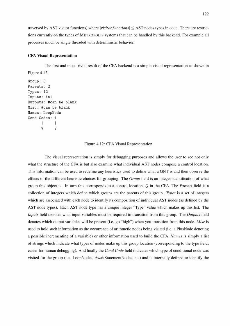
122
traversed by AST visitor functions) where |visitor f unctions| ≤ AST nodes types in code. There are restric-
tions currently on the types of METROPOLIS systems that can be handled by this backend. For example all
processes much be single threaded with deterministic behavior.
CFA Visual Representation
The first and most trivial result of the CFA backend is a simple visual representation as shown in
Figure 4.12.
Group: 3Parents: 2Types: 12Inputs: in1Outputs: #can be blankMisc: #can be blankNames: LoopNodeCond Codes: 1
| |V V
Figure 4.12: CFA Visual Representation
The visual representation is simply for debugging purposes and allows the user to see not only
what the structure of the CFA is but also examine what individual AST nodes compose a control location.
This information can be used to redefine any heuristics used to define what a GNT is and then observe the
effects of the different heuristic choices for grouping. The Group field is an integer identification of what
group this object is. In turn this corresponds to a control location, Q in the CFA. The Parents field is a
collection of integers which define which groups are the parents of this group. Types is a set of integers
which are associated with each node to identify its composition of individual AST nodes (as defined by the
AST node types). Each AST node type has a unique integer “Type” value which makes up this list. The
Inputs field denotes what input variables must be required to transition from this group. The Outputs field
denotes which output variables will be present (i.e. go “high”) when you transition from this node. Misc is
used to hold such information as the occurrence of arithmetic nodes being visited (i.e. a PlusNode denoting
a possible incrementing of a variable) or other information used to build the CFA. Names is simply a list
of strings which indicate what types of nodes make up this group location (corresponding to the type field;
easier for human debugging). And finally the Cond Code field indicates which type of conditional node was
visited for the group (i.e. LoopNodes, AwaitStatementNodes, etc) and is internally defined to identify the
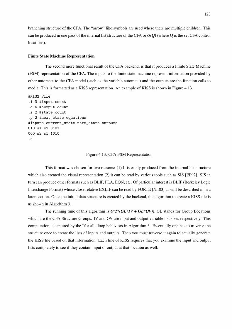
123
branching structure of the CFA. The “arrow” like symbols are used where there are multiple children. This
can be produced in one pass of the internal list structure of the CFA or O(Q) (where Q is the set CFA control
locations).
Finite State Machine Representation
The second more functional result of the CFA backend, is that it produces a Finite State Machine
(FSM) representation of the CFA. The inputs to the finite state machine represent information provided by
other automata to the CFA model (such as the variable automata) and the outputs are the function calls to
media. This is formatted as a KISS representation. An example of KISS is shown in Figure 4.13.
#KISS File.i 3 #input count.o 4 #output count.s 2 #state count.p 2 #next state equations#inputs current_state next_state outputs010 s1 s2 0101000 s2 s1 1010.e
Figure 4.13: CFA FSM Representation
This format was chosen for two reasons: (1) It is easily produced from the internal list structure
which also created the visual representation (2) it can be read by various tools such as SIS [Ell92]. SIS in
turn can produce other formats such as BLIF, PLA, EQN, etc. Of particular interest is BLIF (Berkeley Logic
Interchange Format) whose close relative EXLIF can be read by FORTE [Nir03] as will be described in in a
later section. Once the initial data structure is created by the backend, the algorithm to create a KISS file is
as shown in Algorithm 3.
The running time of this algorithm is O(2*(GL*IV + GL*OV)). GL stands for Group Locations
which are the CFA Structure Groups. IV and OV are input and output variable list sizes respectively. This
computation is captured by the “for all” loop behaviors in Algorithm 3. Essentially one has to traverse the
structure once to create the lists of inputs and outputs. Then you must traverse it again to actually generate
the KISS file based on that information. Each line of KISS requires that you examine the input and output
lists completely to see if they contain input or output at that location as well.
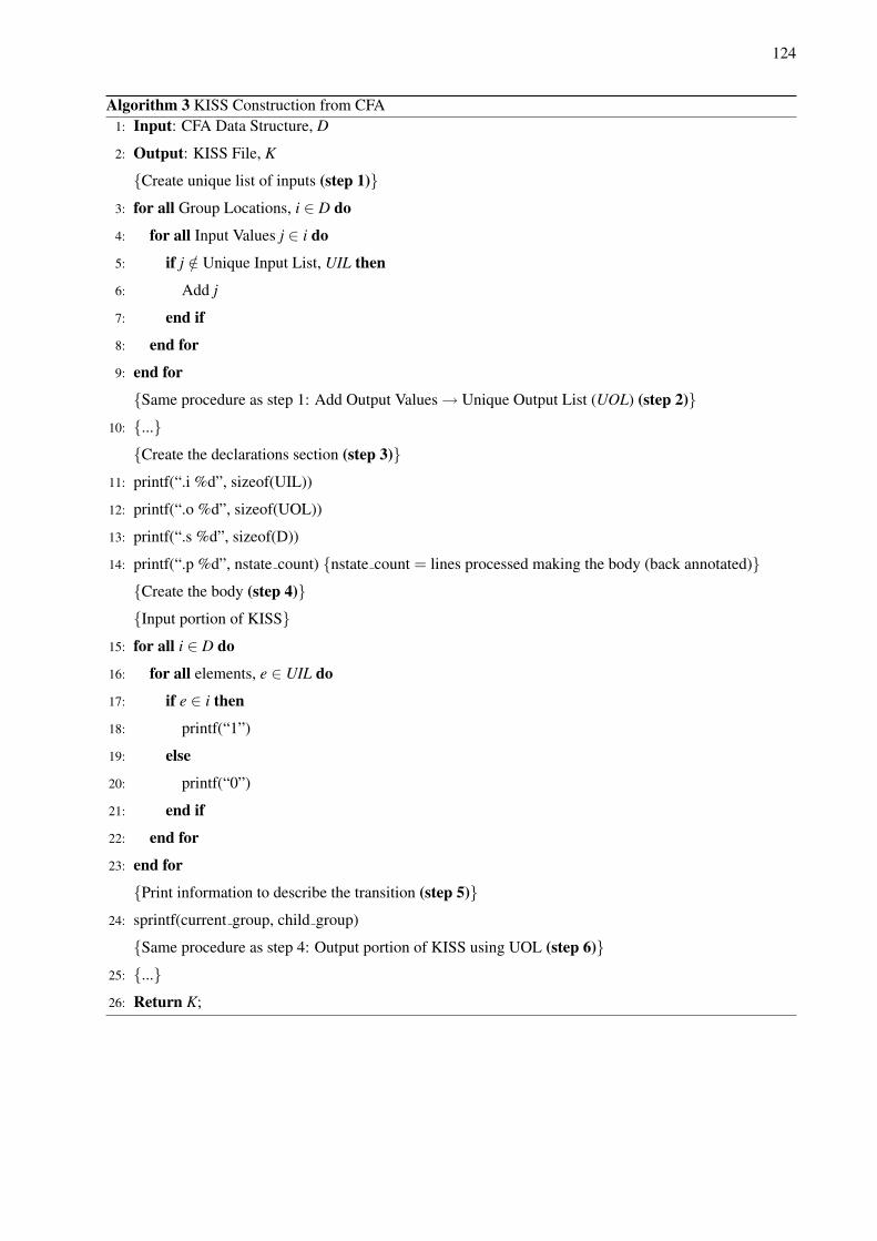
124
Algorithm 3 KISS Construction from CFA1: Input: CFA Data Structure, D
2: Output: KISS File, K
{Create unique list of inputs (step 1)}3: for all Group Locations, i ∈ D do
4: for all Input Values j ∈ i do
5: if j /∈ Unique Input List, UIL then
6: Add j
7: end if
8: end for
9: end for
{Same procedure as step 1: Add Output Values → Unique Output List (UOL) (step 2)}10: {...}
{Create the declarations section (step 3)}11: printf(“.i %d”, sizeof(UIL))
12: printf(“.o %d”, sizeof(UOL))
13: printf(“.s %d”, sizeof(D))
14: printf(“.p %d”, nstate count) {nstate count = lines processed making the body (back annotated)}{Create the body (step 4)}{Input portion of KISS}
15: for all i ∈ D do
16: for all elements, e ∈ UIL do
17: if e ∈ i then
18: printf(“1”)
19: else
20: printf(“0”)
21: end if
22: end for
23: end for
{Print information to describe the transition (step 5)}24: sprintf(current group, child group)
{Same procedure as step 4: Output portion of KISS using UOL (step 6)}25: {...}26: Return K;
125
Reactive Module Representation
The third and final result of the CFA backend is a reactive module [Raj99] file. This is a modeling
language for describing the behavior of hardware and software systems. This file is produced as an additional
benefit of the backend for three reasons: (1) It is very inexpensive to create a reactive module which models
an FSM. (2) It allows for non-deterministic behavior which is not allowed by KISS models provided to
SIS. (3) It can be read by tools such as MOCHA [Raj98]. MOCHA allows a rich set of model checking
algorithms to be run on the CFA model that are useful both for refinement and other verification tasks.
The first point mentioned for making this representation was that it was inexpensive to do from
the FSM representation. Algorithms 4 and 5 give the algorithm to do so.
The process of creating a reactive module file can be done in one pass of the KISS file. The
variable declaration initializations for the module are simply from the KISS input (.i), output (.o), and state
(.s) declarations. The init command is simply another listing of the variables. The largest part of the file, the
update commands, correspond one-to-one with each line in the KISS body. The running time of this process
is naturally O(L) (where L is the number of KISS Lines).
The second reason for using this representation, non-determinism, is inherent in the fact that
multiple guards in a METROPOLIS await statement may be true. Also inherent is that the union of all guard
commands does not have to equal the entire space of the inputs (i.e. a reactive module can be partially
specified). Naturally, KISS currently has deterministic behavior so it will result in a reactive module with
deterministic behavior. However, there is nothing preventing a reactive module from being produced from a
KISS file which would not run in SIS. A CFA could be produced that has non-deterministic behavior simply
with a modification to the backend.
The third and final reason, the verification tool MOCHA, will be discussed in its own section to
follow.
FORTE Accommodations
Prior to the integration of Reactive Modules into the CFA Backend, this thesis was targeting a tool
called FORTE. FORTE [Nir03] is a tool provided by Intel Corporation which is a collection of several tools.
These are Functional Language (FL), Symbolic Trajectory Evaluation (STE), FSM Logic Data Model, and
some circuit drawing tools. FORTE works on circuit descriptions of models. This is was a major factor in
influencing the decision to reduce the CFA into a FSM representation originally.
Once a model has been created as a KISS file, that KISS file is given to the SIS tool. SIS is used
to create a BLIF file with the SIS script shown in Figure 4.14. BLIF representation is very similar to the
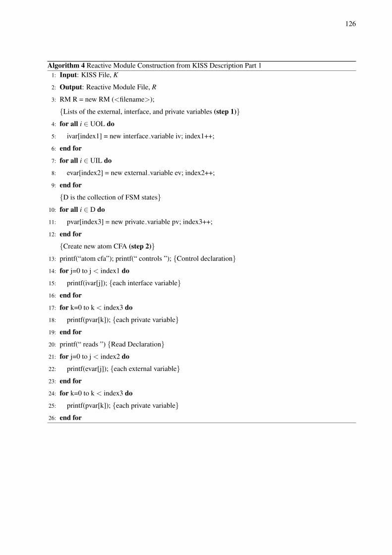
126
Algorithm 4 Reactive Module Construction from KISS Description Part 11: Input: KISS File, K
2: Output: Reactive Module File, R
3: RM R = new RM (<filename>);
{Lists of the external, interface, and private variables (step 1)}4: for all i ∈ UOL do
5: ivar[index1] = new interface variable iv; index1++;
6: end for
7: for all i ∈ UIL do
8: evar[index2] = new external variable ev; index2++;
9: end for
{D is the collection of FSM states}10: for all i ∈ D do
11: pvar[index3] = new private variable pv; index3++;
12: end for
{Create new atom CFA (step 2)}13: printf(“atom cfa”); printf(“ controls ”); {Control declaration}14: for j=0 to j < index1 do
15: printf(ivar[j]); {each interface variable}16: end for
17: for k=0 to k < index3 do
18: printf(pvar[k]); {each private variable}19: end for
20: printf(“ reads ”) {Read Declaration}21: for j=0 to j < index2 do
22: printf(evar[j]); {each external variable}23: end for
24: for k=0 to k < index3 do
25: printf(pvar[k]); {each private variable}26: end for

127
Algorithm 5 Reactive Module Construction from KISS Description Part 21: INPUT: Variable lists and atom CFA from part 1
2: OUTPUT: Reactive Module File, R
{The continuation starting from line 26 of part 1}{Initialize Module (step 3)}
3: printf(“ init ”)
{All interface and private variables = false except first state variable}4: printf(pvar[0] = true);
5: for k=1 to k < index3 do
6: printf(pvar[k] = false);
7: end for
8: for j=0 to j < index1 do
9: printf(ivar[j] = false);
10: end for
{Update Behavior (step 4)}11: printf(“ update ”);
{Pseudo Description}12: <For each line of the KISS representation, the guard is the appropriate input = true and that current
state = true. The result is the next state variable = true and the appropriate outputs = true>
13: Return R;

128
EXLIF file format used by FORTE. EXLIF is an extension of the LIF format in general. The EXLIF holds,
in addition to combinational circuit truth tables, constructs to model sequential elements, like transparent
latches and master slave flip-flops. It has constructs for describing structural hierarchy, tri-state drivers,
various kinds of assertions, etc. Some simple modifications allowed BLIF to be converted to EXLIF and in
turn read by FORTE also shown in Figure 4.14. These manual edits could be worked into a Perl script very
easily.
//sis commandsread_kiss <filename>state_minimizestate_assign <nova> or <jedi>source script.ruggedwrite_blif <filename>
BLIF to EXLIF Manual Edits:
• Remove start kiss, end kiss, and kiss code embedded in file
• Remove external don’t care section (.exdc)
• Add to the .latch definitions a clk signal and the type of flop it is (rising, falling)
• Remove the .latch order and .code portions
Figure 4.14: SIS Commands and EXLIF Requirements for FORTE Flow
Once the models are converted to EXLIF files, FORTE can begin to process them for refinement.
The algorithm which FORTE uses to prove refinement between to EXLIF files is in Algorithm 6.
The running time for such an algorithm is approximately O(m * n) where n is the number of states
and m is the number of transitions. This algorithm (6) and corresponding implementation code was not
created as part of this thesis but supplied by Intel.
MOCHA Accommodations
Since the CFA backend produces a Reactive Module, MOCHA can be used to do refinement
checking as well. However, this process requires some manual preparation of the file produced by the
backend. [Raj98] describes refinement as a trace inclusion problem. To check that X �Re f Y requires:
1. For every initial state, s of X, the projection of s to the variables of Y is an initial state of Y. Basically
they need the same initial state.
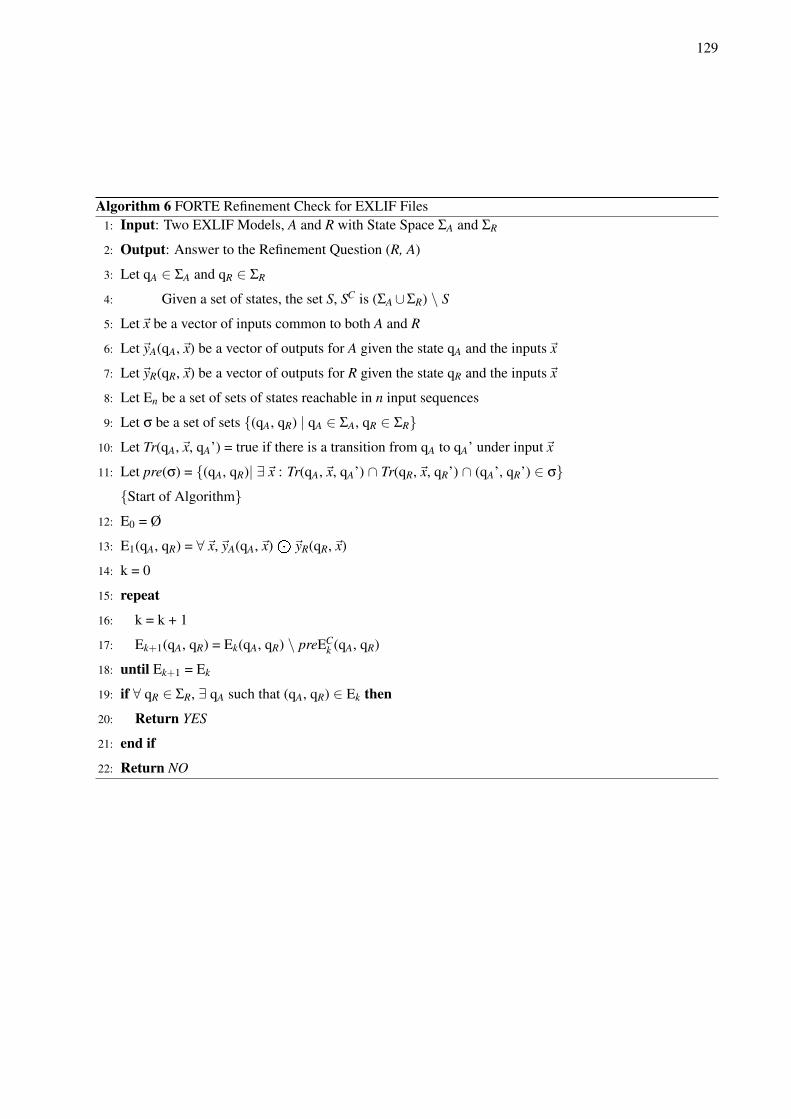
129
Algorithm 6 FORTE Refinement Check for EXLIF Files1: Input: Two EXLIF Models, A and R with State Space ΣA and ΣR
2: Output: Answer to the Refinement Question (R, A)
3: Let qA ∈ ΣA and qR ∈ ΣR
4: Given a set of states, the set S, SC is (ΣA∪ΣR) \ S
5: Let~x be a vector of inputs common to both A and R
6: Let~yA(qA,~x) be a vector of outputs for A given the state qA and the inputs~x
7: Let~yR(qR,~x) be a vector of outputs for R given the state qR and the inputs~x
8: Let En be a set of sets of states reachable in n input sequences
9: Let σ be a set of sets {(qA, qR) | qA ∈ ΣA, qR ∈ ΣR}10: Let Tr(qA,~x, qA’) = true if there is a transition from qA to qA’ under input~x
11: Let pre(σ) = {(qA, qR)| ∃~x : Tr(qA,~x, qA’) ∩ Tr(qR,~x, qR’) ∩ (qA’, qR’) ∈ σ}{Start of Algorithm}
12: E0 = Ø
13: E1(qA, qR) = ∀~x,~yA(qA,~x)J
~yR(qR,~x)
14: k = 0
15: repeat
16: k = k + 1
17: Ek+1(qA, qR) = Ek(qA, qR) \ preECk (qA, qR)
18: until Ek+1 = Ek
19: if ∀ qR ∈ ΣR, ∃ qA such that (qA, qR) ∈ Ek then
20: Return YES
21: end if
22: Return NO

130
2. For every reachable state of s of X, if X has a transition from s to t then Y has a matching transition.
The search can be done symbolically or enumerated with MOCHA. In the case that the test fails, it generates
a counterexample of a trace on X which is not a trace of Y. This may be computationally complex. Therefore
some restrictions are placed on the modules, to verify X �Re f Y.
1. The module Y has no private variables - This requirement has to do with observability.
2. Every interface variable of Y is an interface variable of X - This requirement is a syntactic issue
issue which allows the tool to function without the user explicitly providing a list detailing variable
correspondence.
3. Every external variable of Y is an external variable of X - This requirement is also a syntactic issue.
Recalling the requirements for refinement, the 2nd and 3rd conditions are already met. However,
a module created with the CFA Backend will have private variables representing states. The solution for
this is to create a Witness Module, W. This is a module whose interface variables are the private variables of
Y. Also, W should not contain any of the external variables of X. In turn a module, Y’, will be created with
the original Y’s private variables declared as interface variables. Once this process has been performed then
X||W �Re f Y’ as shown in [Raj99]. The procedure is naturally:
1. Create a module Y’ from Y by changing private variables to interface.
2. Define a Witness Module, W, whose interface variables are the private variables of Y but exclude the
observable (external) variables of X.
3. Check X||W �Re f Y’ with MOCHA
Since this process is not automatic it represents a potential bottleneck in the flow. The creation of a
Witness Module requires creativity on the part of the user since the variable reassignment may be nontrivial
in order to maintain correct functionality. In addition the parallel composition is also manual. There is
much information required to fully understand the MOCHA tool which is not described here. The reader is
referred to the references provided for more information.
Composite Design Flow
In conclusion, in order to demonstrate a proof of concept for this surface refinement methodology,
this thesis assembled the previously described components into a complete flow as shown in Figure 4.15.
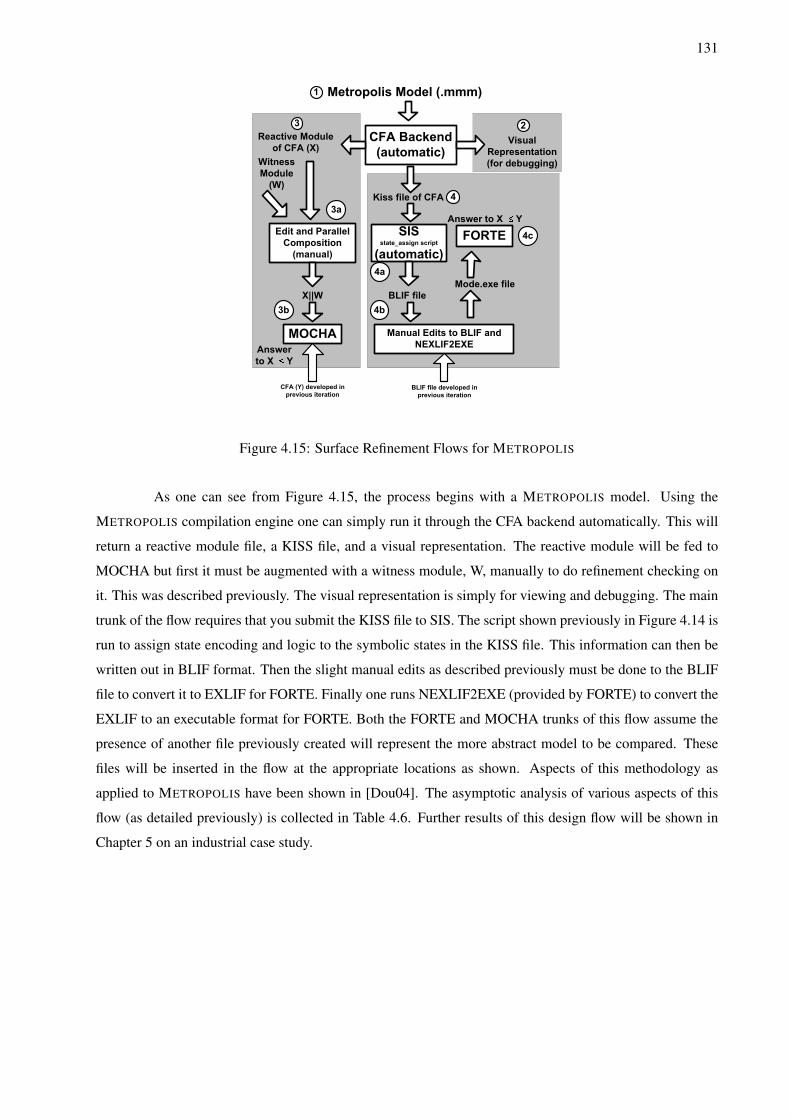
131
Visual
Representation
(for debugging)
Reactive Module
of CFA (X)
Kiss file of CFA
state_assign script
BLIF file
Manual Edits to BLIF and
NEXLIF2EXE
Mode.exe file
Witness
Module
(W)
Edit and Parallel
Composition
(manual)
X||W
1
23
3a
3b
4
4a
4b
4c
Answer
to X Y
Answer to X Y
CFA (Y) developed in
previous iterationBLIF file developed in
previous iteration
Figure 4.15: Surface Refinement Flows for METROPOLIS
As one can see from Figure 4.15, the process begins with a METROPOLIS model. Using the
METROPOLIS compilation engine one can simply run it through the CFA backend automatically. This will
return a reactive module file, a KISS file, and a visual representation. The reactive module will be fed to
MOCHA but first it must be augmented with a witness module, W, manually to do refinement checking on
it. This was described previously. The visual representation is simply for viewing and debugging. The main
trunk of the flow requires that you submit the KISS file to SIS. The script shown previously in Figure 4.14 is
run to assign state encoding and logic to the symbolic states in the KISS file. This information can then be
written out in BLIF format. Then the slight manual edits as described previously must be done to the BLIF
file to convert it to EXLIF for FORTE. Finally one runs NEXLIF2EXE (provided by FORTE) to convert the
EXLIF to an executable format for FORTE. Both the FORTE and MOCHA trunks of this flow assume the
presence of another file previously created will represent the more abstract model to be compared. These
files will be inserted in the flow at the appropriate locations as shown. Aspects of this methodology as
applied to METROPOLIS have been shown in [Dou04]. The asymptotic analysis of various aspects of this
flow (as detailed previously) is collected in Table 4.6. Further results of this design flow will be shown in
Chapter 5 on an industrial case study.
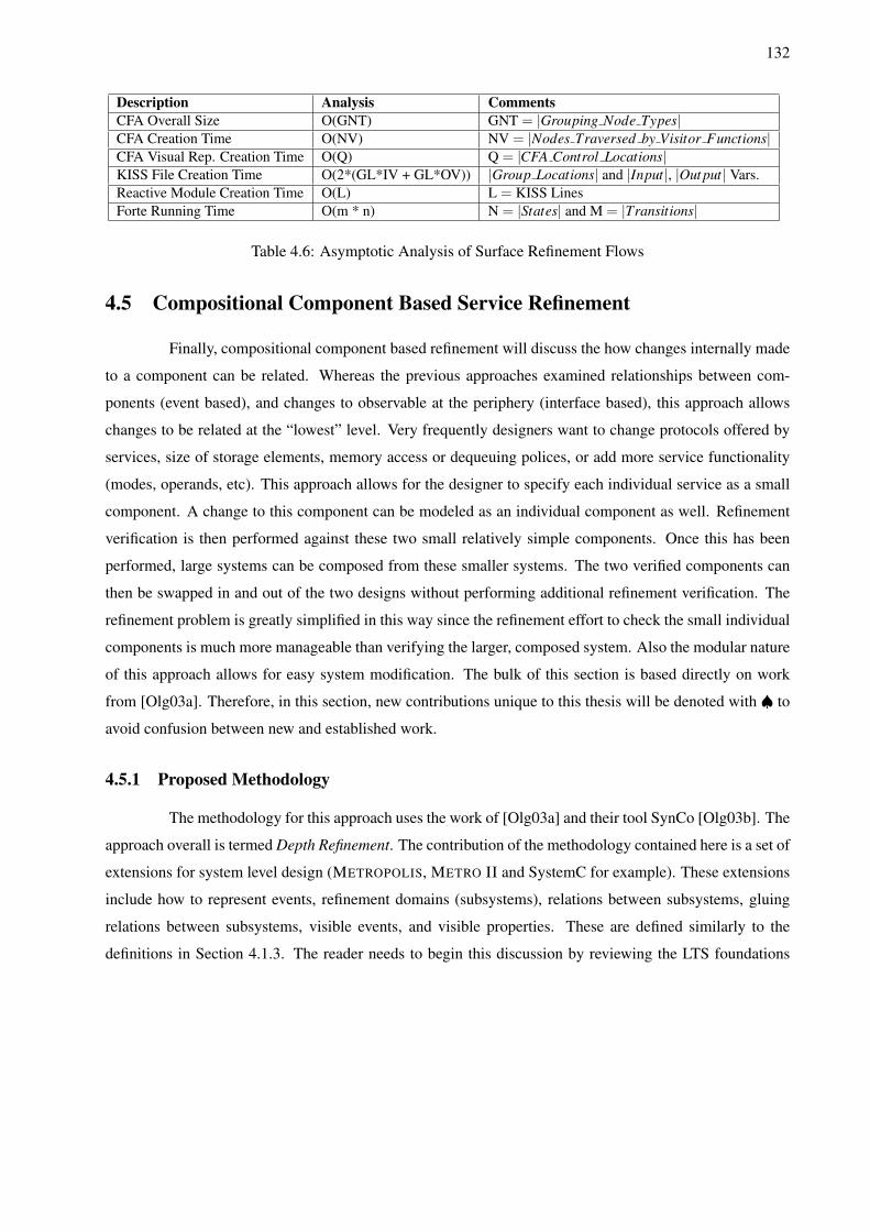
132
Description Analysis CommentsCFA Overall Size O(GNT) GNT = |Grouping Node Types|CFA Creation Time O(NV) NV = |Nodes Traversed by Visitor Functions|CFA Visual Rep. Creation Time O(Q) Q = |CFA Control Locations|KISS File Creation Time O(2*(GL*IV + GL*OV)) |Group Locations| and |Input|, |Out put| Vars.Reactive Module Creation Time O(L) L = KISS LinesForte Running Time O(m * n) N = |States| and M = |Transitions|
Table 4.6: Asymptotic Analysis of Surface Refinement Flows
4.5 Compositional Component Based Service Refinement
Finally, compositional component based refinement will discuss the how changes internally made
to a component can be related. Whereas the previous approaches examined relationships between com-
ponents (event based), and changes to observable at the periphery (interface based), this approach allows
changes to be related at the “lowest” level. Very frequently designers want to change protocols offered by
services, size of storage elements, memory access or dequeuing polices, or add more service functionality
(modes, operands, etc). This approach allows for the designer to specify each individual service as a small
component. A change to this component can be modeled as an individual component as well. Refinement
verification is then performed against these two small relatively simple components. Once this has been
performed, large systems can be composed from these smaller systems. The two verified components can
then be swapped in and out of the two designs without performing additional refinement verification. The
refinement problem is greatly simplified in this way since the refinement effort to check the small individual
components is much more manageable than verifying the larger, composed system. Also the modular nature
of this approach allows for easy system modification. The bulk of this section is based directly on work
from [Olg03a]. Therefore, in this section, new contributions unique to this thesis will be denoted with ♠ to
avoid confusion between new and established work.
4.5.1 Proposed Methodology
The methodology for this approach uses the work of [Olg03a] and their tool SynCo [Olg03b]. The
approach overall is termed Depth Refinement. The contribution of the methodology contained here is a set of
extensions for system level design (METROPOLIS, METRO II and SystemC for example). These extensions
include how to represent events, refinement domains (subsystems), relations between subsystems, gluing
relations between subsystems, visible events, and visible properties. These are defined similarly to the
definitions in Section 4.1.3. The reader needs to begin this discussion by reviewing the LTS foundations
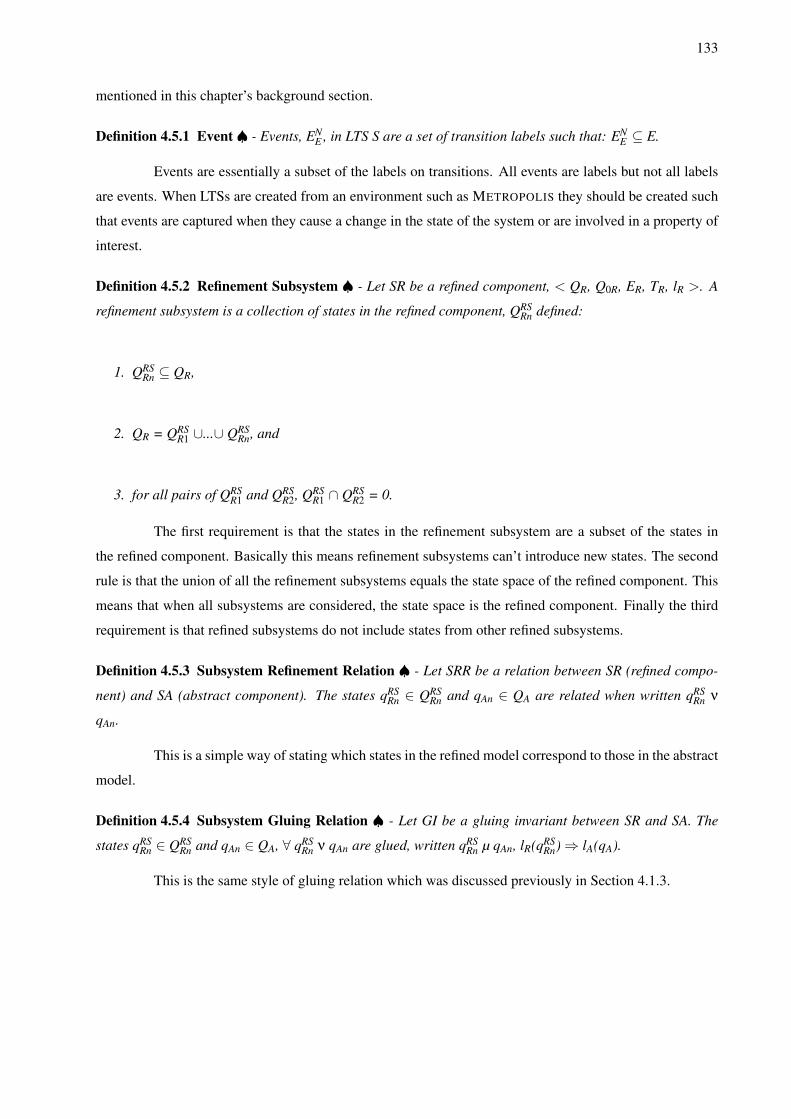
133
mentioned in this chapter’s background section.
Definition 4.5.1 Event ♠ - Events, ENE , in LTS S are a set of transition labels such that: EN
E ⊆ E.
Events are essentially a subset of the labels on transitions. All events are labels but not all labels
are events. When LTSs are created from an environment such as METROPOLIS they should be created such
that events are captured when they cause a change in the state of the system or are involved in a property of
interest.
Definition 4.5.2 Refinement Subsystem ♠ - Let SR be a refined component, < QR, Q0R, ER, TR, lR >. A
refinement subsystem is a collection of states in the refined component, QRSRn defined:
1. QRSRn ⊆ QR,
2. QR = QRSR1 ∪...∪ QRS
Rn, and
3. for all pairs of QRSR1 and QRS
R2, QRSR1 ∩ QRS
R2 = 0.
The first requirement is that the states in the refinement subsystem are a subset of the states in
the refined component. Basically this means refinement subsystems can’t introduce new states. The second
rule is that the union of all the refinement subsystems equals the state space of the refined component. This
means that when all subsystems are considered, the state space is the refined component. Finally the third
requirement is that refined subsystems do not include states from other refined subsystems.
Definition 4.5.3 Subsystem Refinement Relation ♠ - Let SRR be a relation between SR (refined compo-
nent) and SA (abstract component). The states qRSRn ∈ QRS
Rn and qAn ∈ QA are related when written qRSRn ν
qAn.
This is a simple way of stating which states in the refined model correspond to those in the abstract
model.
Definition 4.5.4 Subsystem Gluing Relation ♠ - Let GI be a gluing invariant between SR and SA. The
states qRSRn ∈ QRS
Rn and qAn ∈ QA, ∀ qRSRn ν qAn are glued, written qRS
Rn µ qAn, lR(qRSRn) ⇒ lA(qA).
This is the same style of gluing relation which was discussed previously in Section 4.1.3.
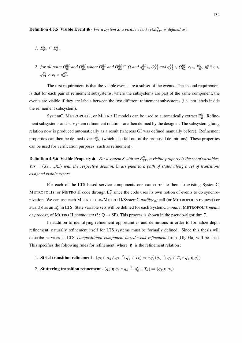
134
Definition 4.5.5 Visible Event ♠ - For a system S, a visible event set,ENEV , is defined as:
1. ENEV ⊆ EN
E ,
2. for all pairs QRSR1 and QRS
R2 where QRSR1 and QRS
R2 ⊆ Q and qRSR1 ∈ QRS
R1 and qRSR2 ∈ QRS
R2, ei ∈ ENEV iff ∃ ti ∈
qRSR1 × ei × qRS
R2.
The first requirement is that the visible events are a subset of the events. The second requirement
is that for each pair of refinement subsystems, where the subsystems are part of the same component, the
events are visible if they are labels between the two different refinement subsystems (i.e. not labels inside
the refinement subsystem).
SystemC, METROPOLIS, or METRO II models can be used to automatically extract ENE . Refine-
ment subsystems and subsystem refinement relations are then defined by the designer. The subsystem gluing
relation now is produced automatically as a result (whereas GI was defined manually before). Refinement
properties can then be defined over ENEV (which also fall out of the proposed definitions). These properties
can be used for verification purposes (such as refinement).
Definition 4.5.6 Visible Property♠ - For a system S with set ENEV , a visible property is the set of variables,
Var = {X1, ...,Xn} with the respective domain, D assigned to a path of states along a set of transitions
assigned visible events.
For each of the LTS based service components one can correlate them to existing SystemC,
METROPOLIS, or METRO II code through ENE since the code uses its own notion of events to do synchro-
nization. We can use each METROPOLIS/METRO II/SystemC notify(en) call (or METROPOLIS request() or
await()) as an EiE in LTS. State variable sets will be defined for each SystemC module, METROPOLIS media
or process, of METRO II component (l : Q → SP). This process is shown in the pseudo-algorithm 7.
In addition to identifying refinement opportunities and definitions in order to formalize depth
refinement, naturally refinement itself for LTS systems must be formally defined. Since this thesis will
describe services as LTS, compositional component based weak refinement from [Olg03a] will be used.
This specifies the following rules for refinement, where η is the refinement relation :
1. Strict transition refinement - (qR η qA∧qRe→ q′R ∈ TR)⇒∃q′A(qA
e→ q′A ∈ TA∧q′R η q′A)
2. Stuttering transition refinement - (qR η qA∧qRτ→ q′R ∈ TR)⇒ (q′R η qA)
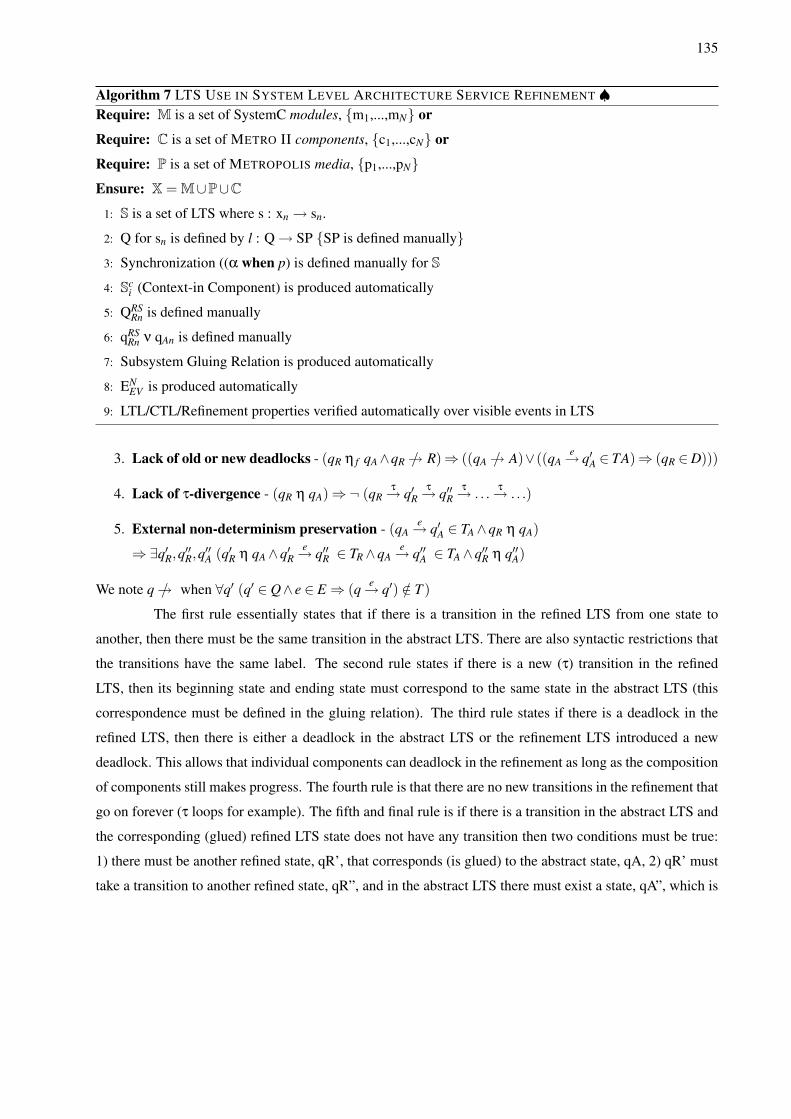
135
Algorithm 7 LTS USE IN SYSTEM LEVEL ARCHITECTURE SERVICE REFINEMENT ♠Require: M is a set of SystemC modules, {m1,...,mN} or
Require: C is a set of METRO II components, {c1,...,cN} or
Require: P is a set of METROPOLIS media, {p1,...,pN}Ensure: X = M∪P∪C
1: S is a set of LTS where s : xn → sn.
2: Q for sn is defined by l : Q → SP {SP is defined manually}3: Synchronization ((α when p) is defined manually for S
4: Sci (Context-in Component) is produced automatically
5: QRSRn is defined manually
6: qRSRn ν qAn is defined manually
7: Subsystem Gluing Relation is produced automatically
8: ENEV is produced automatically
9: LTL/CTL/Refinement properties verified automatically over visible events in LTS
3. Lack of old or new deadlocks - (qR η f qA∧qR →/ R)⇒ ((qA →/ A)∨((qAe→ q′A ∈ TA)⇒ (qR ∈D)))
4. Lack of τ-divergence - (qR η qA)⇒¬ (qRτ→ q′R
τ→ q′′Rτ→ . . .
τ→ . . .)
5. External non-determinism preservation - (qAe→ q′A ∈ TA∧qR η qA)
⇒∃q′R,q′′R,q′′A (q′R η qA∧q′Re→ q′′R ∈ TR∧qA
e→ q′′A ∈ TA∧q′′R η q′′A)
We note q→/ when ∀q′ (q′ ∈ Q∧ e ∈ E ⇒ (q e→ q′) /∈ T )
The first rule essentially states that if there is a transition in the refined LTS from one state to
another, then there must be the same transition in the abstract LTS. There are also syntactic restrictions that
the transitions have the same label. The second rule states if there is a new (τ) transition in the refined
LTS, then its beginning state and ending state must correspond to the same state in the abstract LTS (this
correspondence must be defined in the gluing relation). The third rule states if there is a deadlock in the
refined LTS, then there is either a deadlock in the abstract LTS or the refinement LTS introduced a new
deadlock. This allows that individual components can deadlock in the refinement as long as the composition
of components still makes progress. The fourth rule is that there are no new transitions in the refinement that
go on forever (τ loops for example). The fifth and final rule is if there is a transition in the abstract LTS and
the corresponding (glued) refined LTS state does not have any transition then two conditions must be true:
1) there must be another refined state, qR’, that corresponds (is glued) to the abstract state, qA, 2) qR’ must
take a transition to another refined state, qR”, and in the abstract LTS there must exist a state, qA”, which is
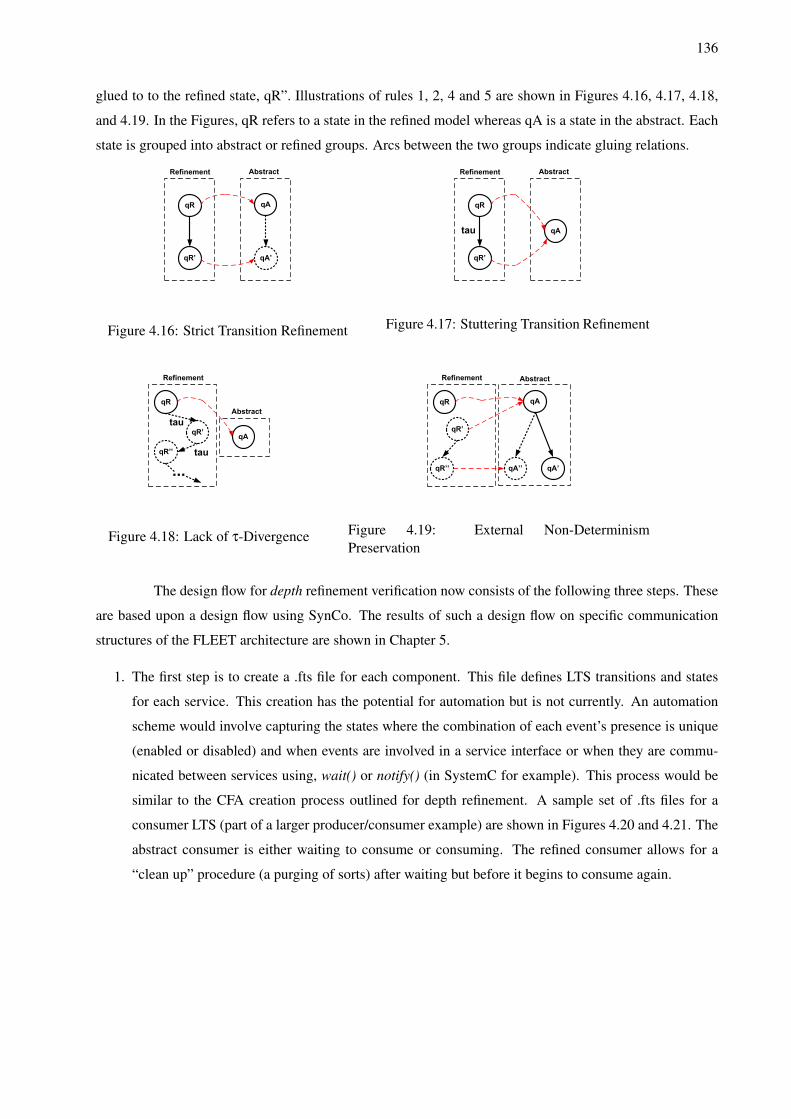
136
glued to to the refined state, qR”. Illustrations of rules 1, 2, 4 and 5 are shown in Figures 4.16, 4.17, 4.18,
and 4.19. In the Figures, qR refers to a state in the refined model whereas qA is a state in the abstract. Each
state is grouped into abstract or refined groups. Arcs between the two groups indicate gluing relations.
qR qA
qA’qR’
Refinement Abstract
Figure 4.16: Strict Transition Refinement
qR
qA
qR’
Refinement Abstract
tau
Figure 4.17: Stuttering Transition Refinement
qR
qAqR’
Refinement
Abstract
tau
qR’’ tau
Figure 4.18: Lack of τ-Divergence
qR qA
qR’
Refinement Abstract
qR’’ qA’qA’’
Figure 4.19: External Non-DeterminismPreservation
The design flow for depth refinement verification now consists of the following three steps. These
are based upon a design flow using SynCo. The results of such a design flow on specific communication
structures of the FLEET architecture are shown in Chapter 5.
1. The first step is to create a .fts file for each component. This file defines LTS transitions and states
for each service. This creation has the potential for automation but is not currently. An automation
scheme would involve capturing the states where the combination of each event’s presence is unique
(enabled or disabled) and when events are involved in a service interface or when they are commu-
nicated between services using, wait() or notify() (in SystemC for example). This process would be
similar to the CFA creation process outlined for depth refinement. A sample set of .fts files for a
consumer LTS (part of a larger producer/consumer example) are shown in Figures 4.20 and 4.21. The
abstract consumer is either waiting to consume or consuming. The refined consumer allows for a
“clean up” procedure (a purging of sorts) after waiting but before it begins to consume again.
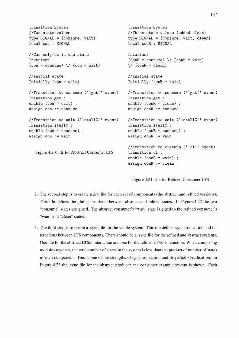
137
Transition System//Two state valuestype SIGNAL = {consume, wait}local con : SIGNAL
//Can only be in one stateInvariant(con = consume) \/ (con = wait)
//Initial stateInitially (con = wait)
//Transition to consume (‘‘get’’ event)Transition get :enable (con = wait) ;assign con := consume
//Transition to wait (‘‘stallC’’ event)Transition stallC :enable (con = consume) ;assign con := wait
Figure 4.20: .fts for Abstract Consumer LTS
Transition System//Three state values (added clean)type SIGNAL = {consume, wait, clean}local conR : SIGNAL
Invariant(conR = consume) \/ (conR = wait)\/ (conR = clean)
//Initial stateInitially (conR = wait)
//Transition to consume (‘‘get’’ event)Transition get :enable (conR = clean) ;assign conR := consume
//Transition to wait (‘‘stallC’’ event)Transition stallC :enable (conR = consume) ;assign conR := wait
//Transition to cleanup (‘‘cl’’ event)Transition cl :enable (conR = wait) ;assign conR := clean
Figure 4.21: .fts for Refined Consumer LTS
2. The second step is to create a .inv file for each set of components (the abstract and refined versions).
This file defines the gluing invariants between abstract and refined states. In Figure 4.22 the two
“consume” states are glued. The abstract consumer’s “wait” state is glued to the refined consumer’s
“wait” and “clean” states.
3. The third step is to create a .sync file for the whole system. This file defines synchronization and in-
teractions between LTS components. There should be a .sync file for the refined and abstract systems.
One file for the abstract LTSs’ interaction and one for the refined LTSs’ interaction. When composing
modules together, the total number of states in the system is less than the product of number of states
in each component. This is one of the strengths of synchronization and its partial specification. In
Figure 4.23 the .sync file for the abstract producer and consumer example system is shown. Each
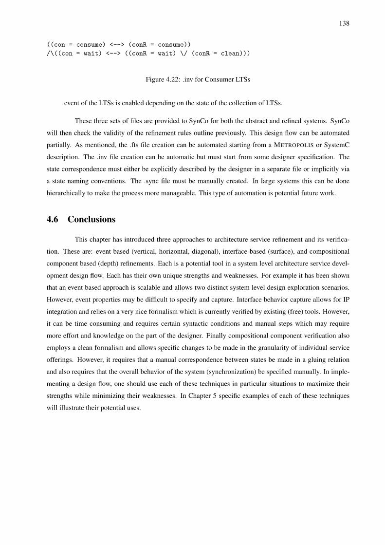
138
((con = consume) <--> (conR = consume))/\((con = wait) <--> ((conR = wait) \/ (conR = clean)))
Figure 4.22: .inv for Consumer LTSs
event of the LTSs is enabled depending on the state of the collection of LTSs.
These three sets of files are provided to SynCo for both the abstract and refined systems. SynCo
will then check the validity of the refinement rules outline previously. This design flow can be automated
partially. As mentioned, the .fts file creation can be automated starting from a METROPOLIS or SystemC
description. The .inv file creation can be automatic but must start from some designer specification. The
state correspondence must either be explicitly described by the designer in a separate file or implicitly via
a state naming conventions. The .sync file must be manually created. In large systems this can be done
hierarchically to make the process more manageable. This type of automation is potential future work.
4.6 Conclusions
This chapter has introduced three approaches to architecture service refinement and its verifica-
tion. These are: event based (vertical, horizontal, diagonal), interface based (surface), and compositional
component based (depth) refinements. Each is a potential tool in a system level architecture service devel-
opment design flow. Each has their own unique strengths and weaknesses. For example it has been shown
that an event based approach is scalable and allows two distinct system level design exploration scenarios.
However, event properties may be difficult to specify and capture. Interface behavior capture allows for IP
integration and relies on a very nice formalism which is currently verified by existing (free) tools. However,
it can be time consuming and requires certain syntactic conditions and manual steps which may require
more effort and knowledge on the part of the designer. Finally compositional component verification also
employs a clean formalism and allows specific changes to be made in the granularity of individual service
offerings. However, it requires that a manual correspondence between states be made in a gluing relation
and also requires that the overall behavior of the system (synchronization) be specified manually. In imple-
menting a design flow, one should use each of these techniques in particular situations to maximize their
strengths while minimizing their weaknesses. In Chapter 5 specific examples of each of these techniques
will illustrate their potential uses.
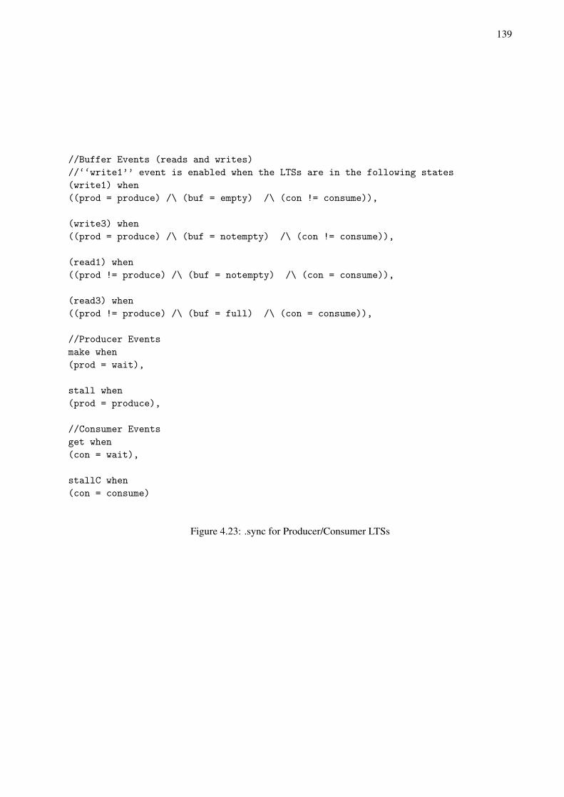
139
//Buffer Events (reads and writes)//‘‘write1’’ event is enabled when the LTSs are in the following states(write1) when((prod = produce) /\ (buf = empty) /\ (con != consume)),
(write3) when((prod = produce) /\ (buf = notempty) /\ (con != consume)),
(read1) when((prod != produce) /\ (buf = notempty) /\ (con = consume)),
(read3) when((prod != produce) /\ (buf = full) /\ (con = consume)),
//Producer Eventsmake when(prod = wait),
stall when(prod = produce),
//Consumer Eventsget when(con = wait),
stallC when(con = consume)
Figure 4.23: .sync for Producer/Consumer LTSs
140
Chapter 5
Design Flow Examples
“Results! Why, man I have gotten a lot of results. I know several thousand things that won’twork.” - Thomas Edison, Inventor
Earlier in the description of this thesis’ goals, claims were made regarding the accuracy and
efficiency of the proposed design flow. Previous chapters have gone into great detail regarding the design
flow. Particularly the development of system level architecture services has been described (Chapter 2), their
characterization (Chapter 3), and finally their refinement (Chapter 4). These chapters have shown the level
of abstraction possible as well as this design flow’s modularity. This chapter will now specifically show
how each of those approaches maintained the accuracy and efficiency needed by ESL tools for adoption by
the larger EDA industry. This demonstration will be done through a series of case studies each designed to
highlight a particular aspect of the design flow outlined.
Accuracy and Efficiency Interpretations
Before discussing the case studies, it is important to understand what the is meant both by accuracy
as well as efficiency. Formally accuracy is defined [Mer07] as: “degree of conformity of a measure to a
standard or a true value”. In the case of design space exploration of embedded systems, the “standard or
true value” is the value that would be obtained by the actual implementation of the design. For example, if
one where to create a model of an image processing system, an accurate model would be one in which the
predicted execution time obtained by simulation was close to the actual value of the existing system. How
close is “acceptable” depends on a variety of factors. One factor is the domain of the design. For example,
safety critical systems such as avionics or medical systems may require very little deviation. Another factor
is what quantity is being measured. For some systems, memory usage may need to be very exact (small
embedded devices for example) while for others it may not be as important (super computer systems for
141
example). A 1% error may be a large deviation for some measurements, while 30% acceptable for others.
Finally, acceptable accuracy will depend on the level of abstraction. More abstract systems typically require
less accuracy because they are usually concerned with making broad system level decisions and increasing
accuracy is not only not required (design simulation speed is more desirable) but also potentialy not possible.
Since accuracy is such a contextual concept, this work requires accuracy to the extent that
fidelity holds. Fidelity was defined in Chapter 1 as a required ordering of measurements. This property
does not mean more accurate measurements necessarily. For example consider three systems A, B, and C.
Assume the actual execution time for A is 3 seconds, B 2 seconds, and C 5 seconds. Therefore the ordering
from fastest to slowest is B, A, C. Consider a very accurate simulation which reports A as 2.7 seconds,
B as 2.8 seconds, and C as 5.1 seconds. This ordering would be A, B, C. While the average error of the
measurements is 0.4 seconds, fidelity does not hold. Contrast this with a highly inaccurate system which
predicts A as 100 seconds, B as 50 seconds, and C as 200 seconds. The average error is much higher (113
seconds) but the system ordering is correctly B, A, C. In the case studies to follow, this ordering or fidelity
is maintained in all cases. In addition average accuracy is quite good as well which is also desirable since
for the systems that do require accuracy, the designer will have a good feel for the viability of the design.
The second concern, efficiency, again has many various meanings when discussing tool devel-
opment. Primarily it has two interpretations. The first refers to how easily a designer can express his/her
desires. For example, a system defined more efficiently by this definition may result in less lines of code,
more library functions, or a larger design library. The result of being more efficient in this space will result
in a design being completed faster (although not necessarily correctly which is why efficiency is only one
part of the proposed design flow). The second interpretation of efficiency has to do with the running time of
the tool. A more efficient tool will take less time to simulate a design. This is accomplished by using careful
programming techniques and algorithms with low asymptotic running times. In this work, the second inter-
pretation is what is of importance. In all cases, the running time of the design flow implemented is as fast or
no more than 20% slower than competing approachs.
The contribution of the four case studies presented in this chapter is a demonstration of the proposed
design flow’s use of specific modeling techniques, characterization of programmable platforms, and
refinement verification to ensure design point fidelity while maintaining a simulation running time no more
than 20% slower than competing approaches.
142
5.0.1 Chapter Organization
This chapter is organized around four case studies. The first case study presented in Section 5.1 is
an exploration of four potential Motion-JPEG (MJPEG) encoder implementations. This example is provided
to show how the characterization process from Chapter 3 is superior than using area based estimations (the
naıve method). The second exploration in Section 5.2 models an H.264 deblocking filter and is meant to
demonstrate the modularity in which the architecture service were created allows for a variety of mapping
scenarios for various functional models. The third exploration in Section 5.3 demonstrates how the topology
of an architecture model can be changed, remapped and the resulting behavior of the system still be verified
to be a refinement of the previous, more abstract mapped instance. This is a combination of “vertical” and
“surface” refinement discussed in Chapter 4. The final demonstration in Section 5.4 contrasts the previous
section by performing refinement without changing the topology but by simply replacing services with other
services. The services being replaced are more abstract while the service being used in the replacement are
more refined. This requires that the overall system behavior be preserved after the change. This process was
described as “depth” refinement in Chapter 4.
5.1 Characterization Aided Fidelity Example: Motion-JPEG
To demonstrate how a programmable platform performance characterization method can be used
to make correct decisions during design space exploration, the following multimedia example is provided.
This example deals with evaluating various architecture topologies and illustrates the importance of accu-
racy in characterization and exemplifies the fidelity achieved with the proposed design flow’s method. In
an exploration like this one, the designer is interested in choosing the design with the best performance.
Therefore it is not as important that the exact performance be known, but rather that the ordering of the
performances amongst the candidates is correct (hence the emphasis on fidelity). Without the methods cov-
ered in this thesis, estimated values would be used to inform the designer of the predicted performance.
These values may come from datasheets, previous simulations, or even best guesses (techniques described
in Chapter 2, Section 2.4). None of these are preferable to actual characterization as will be shown.
The application chosen was Motion-JPEG (MJPEG) [Gre91] encoding and both the functional
model and architectural service models were created in the METROPOLIS design environment. Investigated
are four MJPEG architectural service models. A single functional model was created in METROPOLIS which
isolated various levels of task concurrency between the DCT, Quantization, and Huffman processes present
in the application. These aspects of the functional model were then mapped to the architectural model. The
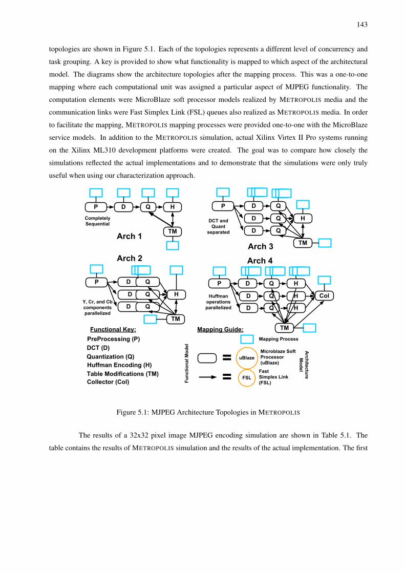
143
topologies are shown in Figure 5.1. Each of the topologies represents a different level of concurrency and
task grouping. A key is provided to show what functionality is mapped to which aspect of the architectural
model. The diagrams show the architecture topologies after the mapping process. This was a one-to-one
mapping where each computational unit was assigned a particular aspect of MJPEG functionality. The
computation elements were MicroBlaze soft processor models realized by METROPOLIS media and the
communication links were Fast Simplex Link (FSL) queues also realized as METROPOLIS media. In order
to facilitate the mapping, METROPOLIS mapping processes were provided one-to-one with the MicroBlaze
service models. In addition to the METROPOLIS simulation, actual Xilinx Virtex II Pro systems running
on the Xilinx ML310 development platforms were created. The goal was to compare how closely the
simulations reflected the actual implementations and to demonstrate that the simulations were only truly
useful when using our characterization approach.
PreProcessing (P)
Huffman Encoding (H)
DCT (D)
Quantization (Q)
P D Q H P D Q
HD
D Q
Q
P D Q
HD
D Q
Q
H
H
Mapping Guide:
uBlaze
Fast
Simplex Link
(FSL)
TM
Table Modifications (TM)
TM
P D Q
HD
D Q
Q
TM
TM
Col
Functional Key:
FSL
Microblaze Soft
Processor
(uBlaze)
Completely
Sequential
Y, Cr, and Cb
components
parallelized
DCT and
Quant
separated
Huffman
operations
parallelized
Functional Model
Architecture
Model
Mapping Process
Collector (Col)
Figure 5.1: MJPEG Architecture Topologies in METROPOLIS
The results of a 32x32 pixel image MJPEG encoding simulation are shown in Table 5.1. The
table contains the results of METROPOLIS simulation and the results of the actual implementation. The first
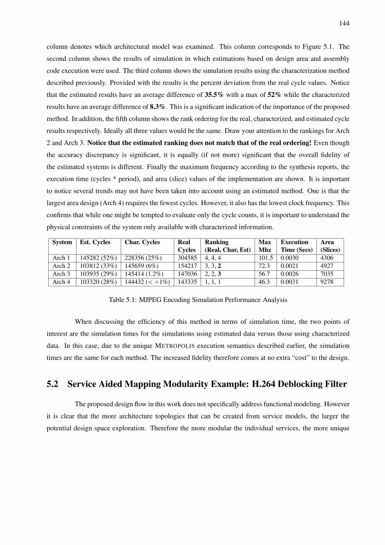
144
column denotes which architectural model was examined. This column corresponds to Figure 5.1. The
second column shows the results of simulation in which estimations based on design area and assembly
code execution were used. The third column shows the simulation results using the characterization method
described previously. Provided with the results is the percent deviation from the real cycle values. Notice
that the estimated results have an average difference of 35.5% with a max of 52% while the characterized
results have an average difference of 8.3%. This is a significant indication of the importance of the proposed
method. In addition, the fifth column shows the rank ordering for the real, characterized, and estimated cycle
results respectively. Ideally all three values would be the same. Draw your attention to the rankings for Arch
2 and Arch 3. Notice that the estimated ranking does not match that of the real ordering! Even though
the accuracy discrepancy is significant, it is equally (if not more) significant that the overall fidelity of
the estimated systems is different. Finally the maximum frequency according to the synthesis reports, the
execution time (cycles * period), and area (slice) values of the implementation are shown. It is important
to notice several trends may not have been taken into account using an estimated method. One is that the
largest area design (Arch 4) requires the fewest cycles. However, it also has the lowest clock frequency. This
confirms that while one might be tempted to evaluate only the cycle counts, it is important to understand the
physical constraints of the system only available with characterized information.
System Est. Cycles Char. Cycles Real Ranking Max Execution AreaCycles (Real, Char, Est) Mhz Time (Secs) (Slices)
Arch 1 145282 (52%) 228356 (25%) 304585 4, 4, 4 101.5 0.0030 4306Arch 2 103812 (33%) 145659 (6%) 154217 3, 3, 2 72.3 0.0021 4927Arch 3 103935 (29%) 145414 (1.2%) 147036 2, 2, 3 56.7 0.0026 7035Arch 4 103320 (28%) 144432 (< +1%) 143335 1, 1, 1 46.3 0.0031 9278
Table 5.1: MJPEG Encoding Simulation Performance Analysis
When discussing the efficiency of this method in terms of simulation time, the two points of
interest are the simulation times for the simulations using estimated data versus those using characterized
data. In this case, due to the unique METROPOLIS execution semantics described earlier, the simulation
times are the same for each method. The increased fidelity therefore comes at no extra “cost” to the design.
5.2 Service Aided Mapping Modularity Example: H.264 Deblocking Filter
The proposed design flow in this work does not specifically address functional modeling. However
it is clear that the more architecture topologies that can be created from service models, the larger the
potential design space exploration. Therefore the more modular the individual services, the more unique
145
interactions that can be explored and hence more topologies can be created. This section will demonstrate
the advantages of this modularity and show how unique design points can be analyzed with a high level of
accuracy.
The first stage of this process is the functional modeling of an application. Functional model
exploration is twofold. The first stage is behavior capture. This is the process of examining the various
ways to express the behavior of an application. An important area of exploration is the examination of the
various levels of concurrency which can be present in an application. This process is covered in [Shi06]
using an algebraic representation. This process will not be discussed in depth here and the reader is directed
to read the provided reference for more information. For this work it is sufficient to understand that certain
aspects of an application can occur in parallel. These parallel aspects can then also be sequentialized. Given
all the operations in a design, each can be classified as sequential or parallel in relation to each other. The
design space then becomes the manipulation of these relationships and the partitioning of the sets in which
these relationships are considered. Sequential operations can be executed on one service while parallelism
requires a service for each parallel operation.
The second stage is to take one of the candidate functional representations and assigned aspects
of the functionality to architectural services which compose a architecture instance. This is mapping in
METROPOLIS. This requires a methodology to partition the functional model (this is the first stage [Shi06])
as well as a set of architecture components (as shown in Chapter 2). The METROPOLIS framework then
evaluates potential performance by mapping the functional model onto an architectural model for simulation.
The architecture models for this flow are based on the Xilinx Virtex II Pro FPGA platform [Xil02] created
in METROPOLIS. These models were described in Chapter 2. Specifically this thesis will be examining
architectures based on MicroBlaze soft-microprocessor cores and Fast Simplex Links (FSLs). An FSL is
a FIFO-like communication channel, which connects two MicroBlazes in a point-to-point manner. These
components were selected because they can easily correspond to dataflow applications like the one to be
presented. Because of the way in which these models were created, this section will demonstrate that any
functional model that could be created using the algebraic methods, can be presented with a corresponding
architecture model for a one-to-one mapping.
What will follow is a discussion of the application details, how mapping is performed, and an
analysis of the results obtained.
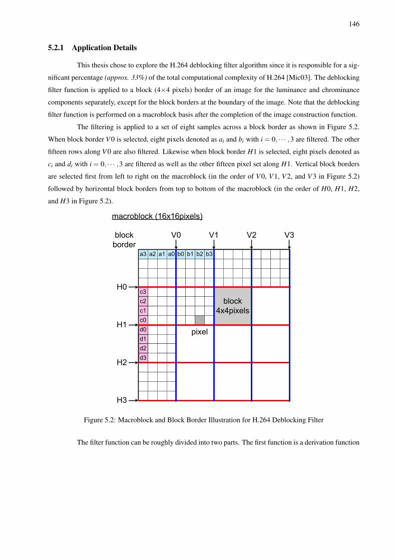
146
5.2.1 Application Details
This thesis chose to explore the H.264 deblocking filter algorithm since it is responsible for a sig-
nificant percentage (approx. 33%) of the total computational complexity of H.264 [Mic03]. The deblocking
filter function is applied to a block (4×4 pixels) border of an image for the luminance and chrominance
components separately, except for the block borders at the boundary of the image. Note that the deblocking
filter function is performed on a macroblock basis after the completion of the image construction function.
The filtering is applied to a set of eight samples across a block border as shown in Figure 5.2.
When block border V 0 is selected, eight pixels denoted as ai and bi with i = 0, · · · ,3 are filtered. The other
fifteen rows along V 0 are also filtered. Likewise when block border H1 is selected, eight pixels denoted as
ci and di with i = 0, · · · ,3 are filtered as well as the other fifteen pixel set along H1. Vertical block borders
are selected first from left to right on the macroblock (in the order of V 0, V 1, V 2, and V 3 in Figure 5.2)
followed by horizontal block borders from top to bottom of the macroblock (in the order of H0, H1, H2,
and H3 in Figure 5.2).
Figure 5.2: Macroblock and Block Border Illustration for H.264 Deblocking Filter
The filter function can be roughly divided into two parts. The first function is a derivation function
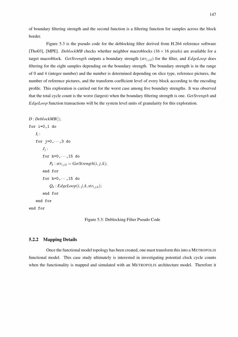
147
of boundary filtering strength and the second function is a filtering function for samples across the block
border.
Figure 5.3 is the pseudo code for the deblocking filter derived from H.264 reference software
[Tho03], [MPE]. DeblockMB checks whether neighbor macroblocks (16× 16 pixels) are available for a
target macroblock. GetStrength outputs a boundary strength (stri, j,k) for the filter, and EdgeLoop does
filtering for the eight samples depending on the boundary strength. The boundary strength is in the range
of 0 and 4 (integer number) and the number is determined depending on slice type, reference pictures, the
number of reference pictures, and the transform coefficient level of every block according to the encoding
profile. This exploration is carried out for the worst case among five boundary strengths. It was observed
that the total cycle count is the worst (largest) when the boundary filtering strength is one. GetStrength and
EdgeLoop function transactions will be the system level units of granularity for this exploration.
D : DeblockMB();
for i=0,1 do
Ii :
for j=0,· · ·,3 do
J j :
for k=0,· · ·,15 do
Pk : stri, j,k = GetStrength(i, j,k);
end for
for k=0,· · ·,15 do
Qk : EdgeLoop(i, j,k,stri, j,k);
end for
end for
end for
Figure 5.3: Deblocking Filter Pseudo Code
5.2.2 Mapping Details
Once the functional model topology has been created, one must transform this into a METROPOLIS
functional model. This case study ultimately is interested in investigating potential clock cycle counts
when the functionality is mapped and simulated with an METROPOLIS architecture model. Therefore it
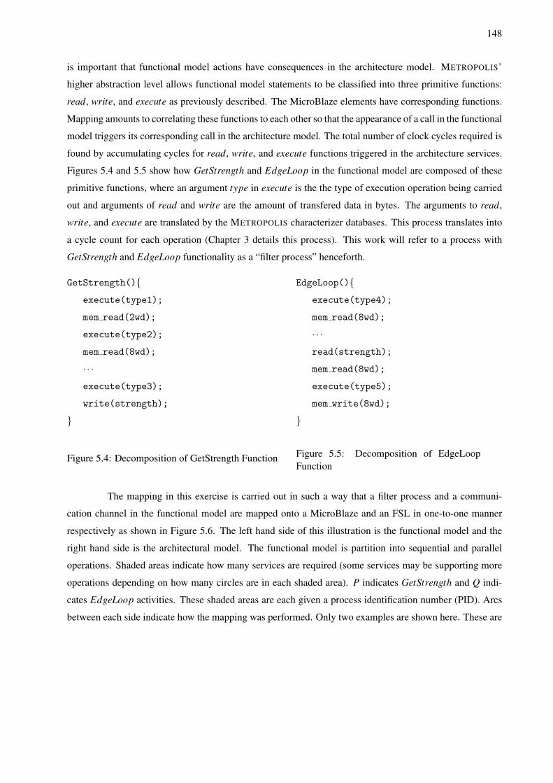
148
is important that functional model actions have consequences in the architecture model. METROPOLIS’
higher abstraction level allows functional model statements to be classified into three primitive functions:
read, write, and execute as previously described. The MicroBlaze elements have corresponding functions.
Mapping amounts to correlating these functions to each other so that the appearance of a call in the functional
model triggers its corresponding call in the architecture model. The total number of clock cycles required is
found by accumulating cycles for read, write, and execute functions triggered in the architecture services.
Figures 5.4 and 5.5 show how GetStrength and EdgeLoop in the functional model are composed of these
primitive functions, where an argument type in execute is the the type of execution operation being carried
out and arguments of read and write are the amount of transfered data in bytes. The arguments to read,
write, and execute are translated by the METROPOLIS characterizer databases. This process translates into
a cycle count for each operation (Chapter 3 details this process). This work will refer to a process with
GetStrength and EdgeLoop functionality as a “filter process” henceforth.
GetStrength(){execute(type1);
mem read(2wd);
execute(type2);
mem read(8wd);
· · ·execute(type3);
write(strength);
}
Figure 5.4: Decomposition of GetStrength Function
EdgeLoop(){execute(type4);
mem read(8wd);
· · ·read(strength);
mem read(8wd);
execute(type5);
mem write(8wd);
}
Figure 5.5: Decomposition of EdgeLoopFunction
The mapping in this exercise is carried out in such a way that a filter process and a communi-
cation channel in the functional model are mapped onto a MicroBlaze and an FSL in one-to-one manner
respectively as shown in Figure 5.6. The left hand side of this illustration is the functional model and the
right hand side is the architectural model. The functional model is partition into sequential and parallel
operations. Shaded areas indicate how many services are required (some services may be supporting more
operations depending on how many circles are in each shaded area). P indicates GetStrength and Q indi-
cates EdgeLoop activities. These shaded areas are each given a process identification number (PID). Arcs
between each side indicate how the mapping was performed. Only two examples are shown here. These are
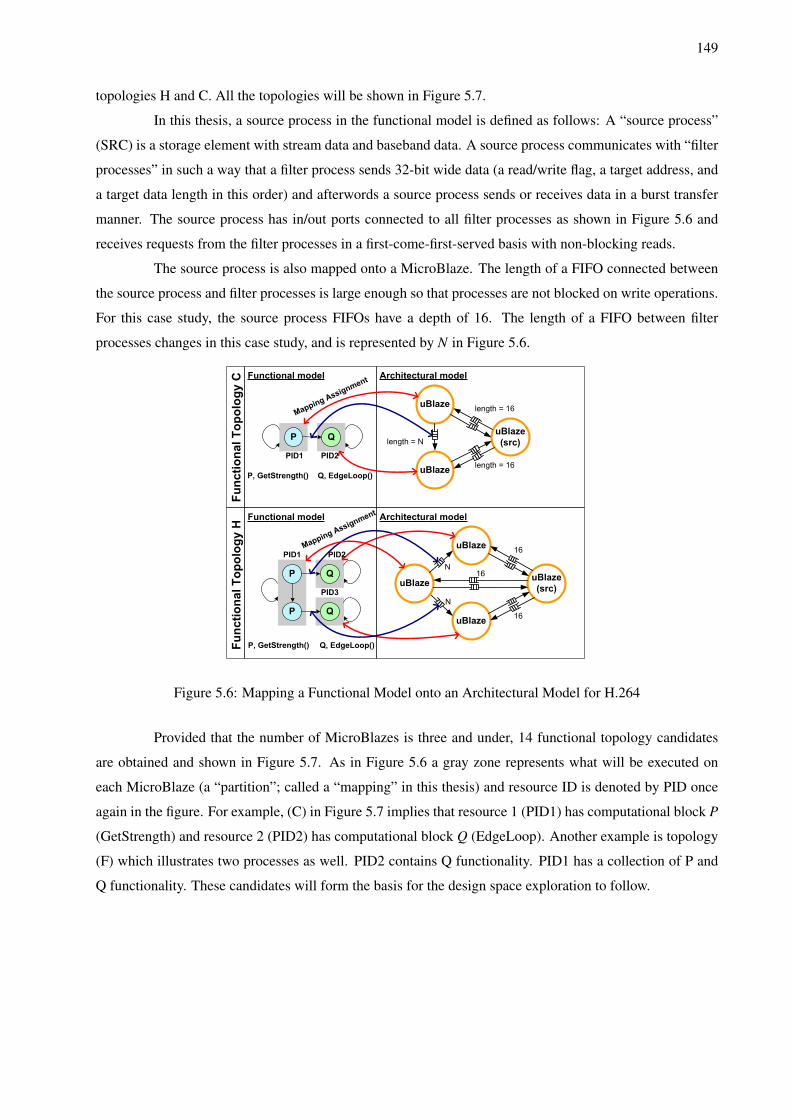
149
topologies H and C. All the topologies will be shown in Figure 5.7.
In this thesis, a source process in the functional model is defined as follows: A “source process”
(SRC) is a storage element with stream data and baseband data. A source process communicates with “filter
processes” in such a way that a filter process sends 32-bit wide data (a read/write flag, a target address, and
a target data length in this order) and afterwords a source process sends or receives data in a burst transfer
manner. The source process has in/out ports connected to all filter processes as shown in Figure 5.6 and
receives requests from the filter processes in a first-come-first-served basis with non-blocking reads.
The source process is also mapped onto a MicroBlaze. The length of a FIFO connected between
the source process and filter processes is large enough so that processes are not blocked on write operations.
For this case study, the source process FIFOs have a depth of 16. The length of a FIFO between filter
processes changes in this case study, and is represented by N in Figure 5.6.
P Q
P Q
uBlaze
uBlaze
uBlaze
(src)uBlaze
P Q
uBlaze
uBlaze
uBlaze
(src)
PID1 PID2
PID1
PID3
PID2
Functional model Architectural model
Functional model Architectural model
length = 16
length = 16
length = N
16
16
16N
N
Mapping Assignment
Mapping Assignment
Q, EdgeLoop()P, GetStrength()
Q, EdgeLoop()P, GetStrength()
Fu
nc
tio
nal
To
po
log
y C
Fu
nc
tio
na
l T
op
olo
gy
H
Figure 5.6: Mapping a Functional Model onto an Architectural Model for H.264
Provided that the number of MicroBlazes is three and under, 14 functional topology candidates
are obtained and shown in Figure 5.7. As in Figure 5.6 a gray zone represents what will be executed on
each MicroBlaze (a “partition”; called a “mapping” in this thesis) and resource ID is denoted by PID once
again in the figure. For example, (C) in Figure 5.7 implies that resource 1 (PID1) has computational block P
(GetStrength) and resource 2 (PID2) has computational block Q (EdgeLoop). Another example is topology
(F) which illustrates two processes as well. PID2 contains Q functionality. PID1 has a collection of P and
Q functionality. These candidates will form the basis for the design space exploration to follow.
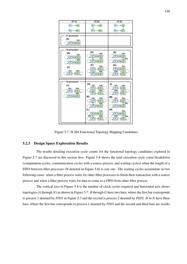
150
(T-1) (T-2) (T-3)
P Q
(A)
P Q
P Q
(B)
P Q
P Q
(D)
P Q
P Q
(E)
P Q
P Q
(F)
P Q
P Q
(G)
PID1
P Q
(C)
<2-process>
<1-process>
P Q
P Q
(I)
P Q
P Q
(J)
P Q
P Q
(K)
P Q
P Q
(M)
P Q
P Q
(L)
P Q
P Q
(N)
P Q
P Q
(H)<3-process>
Pn Qn
Qn-1Pn-1
Pn Qn
Qn-1Pn-1
Pn Qn
Qn-1Pn-1
PID1
PID2
PID1 PID2
PID1
PID2
PID1
PID2
PID1
PID2
PID1
PID2
PID1 PID2
PID3
PID1 PID2
PID3
PID1 PID2
PID3
PID1 PID2
PID3
PID1
PID2
PID3
PID1 PID2
PID3 PID3
PID1 PID2
Figure 5.7: H.264 Functional Topology Mapping Candidates
5.2.3 Design Space Exploration Results
The results detailing execution cycle counts for the functional topology candidates explored in
Figure 5.7 are discussed in this section first. Figure 5.8 shows the total execution cycle count breakdown
(computation cycles, communication cycles with a source process, and waiting cycles) when the length of a
FIFO between filter processes (N denoted in Figure 5.6) is size one. The waiting cycles accumulate in two
following cases: when a filter process waits for other filter processes to finish their transaction with a source
process and when a filter process waits for data to come to a FIFO from other filter process.
The vertical axis in Figure 5.8 is the number of clock cycles required and horizontal axis shows
topologies (A through N) as shown in Figure 5.7. B through G have two bars, where the first bar corresponds
to process 1 denoted by PID1 in Figure 5.7 and the second is process 2 denoted by PID2. H to N have three
bars, where the first bar corresponds to process 1 denoted by PID1 and the second and third bars are results
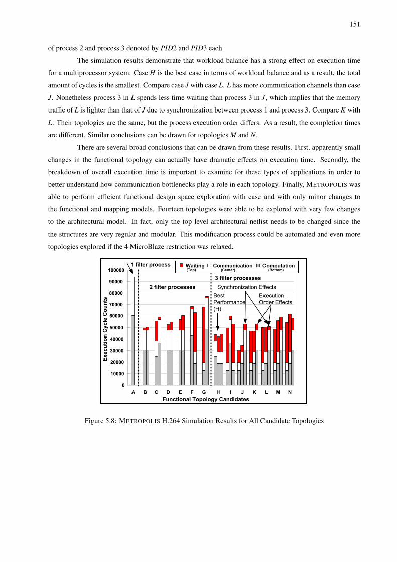
151
of process 2 and process 3 denoted by PID2 and PID3 each.
The simulation results demonstrate that workload balance has a strong effect on execution time
for a multiprocessor system. Case H is the best case in terms of workload balance and as a result, the total
amount of cycles is the smallest. Compare case J with case L. L has more communication channels than case
J. Nonetheless process 3 in L spends less time waiting than process 3 in J, which implies that the memory
traffic of L is lighter than that of J due to synchronization between process 1 and process 3. Compare K with
L. Their topologies are the same, but the process execution order differs. As a result, the completion times
are different. Similar conclusions can be drawn for topologies M and N.
There are several broad conclusions that can be drawn from these results. First, apparently small
changes in the functional topology can actually have dramatic effects on execution time. Secondly, the
breakdown of overall execution time is important to examine for these types of applications in order to
better understand how communication bottlenecks play a role in each topology. Finally, METROPOLIS was
able to perform efficient functional design space exploration with ease and with only minor changes to
the functional and mapping models. Fourteen topologies were able to be explored with very few changes
to the architectural model. In fact, only the top level architectural netlist needs to be changed since the
the structures are very regular and modular. This modification process could be automated and even more
topologies explored if the 4 MicroBlaze restriction was relaxed.
0
10000
20000
30000
40000
50000
60000
70000
80000
90000
100000
A B C D E F G H I J K L M N
1 filter process
2 filter processes
3 filter processes
Execution Cycle Counts
Functional Topology Candidates
Best
Performance
(H)
Execution
Order Effects
Waiting Communication Computation
Synchronization Effects
(Bottom)(Center)(Top)
Figure 5.8: METROPOLIS H.264 Simulation Results for All Candidate Topologies
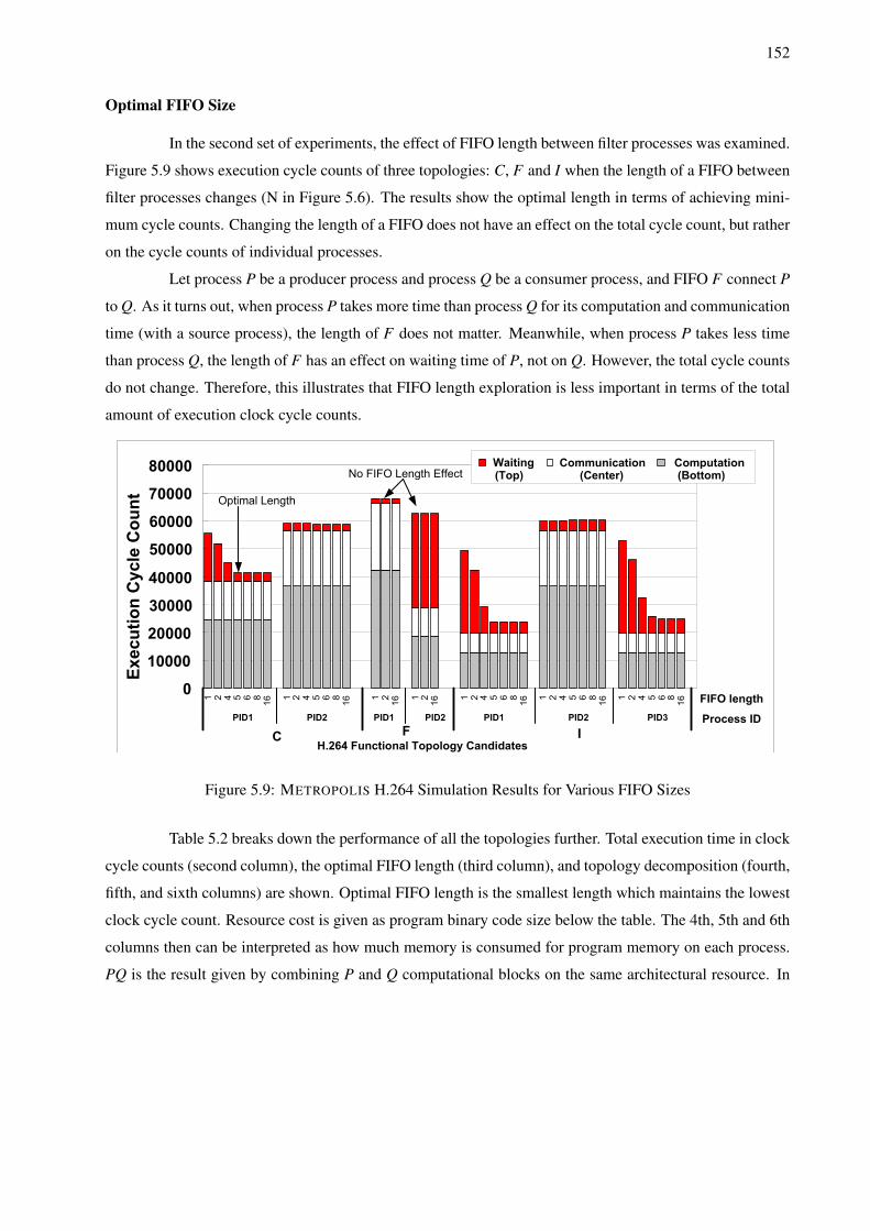
152
Optimal FIFO Size
In the second set of experiments, the effect of FIFO length between filter processes was examined.
Figure 5.9 shows execution cycle counts of three topologies: C, F and I when the length of a FIFO between
filter processes changes (N in Figure 5.6). The results show the optimal length in terms of achieving mini-
mum cycle counts. Changing the length of a FIFO does not have an effect on the total cycle count, but rather
on the cycle counts of individual processes.
Let process P be a producer process and process Q be a consumer process, and FIFO F connect P
to Q. As it turns out, when process P takes more time than process Q for its computation and communication
time (with a source process), the length of F does not matter. Meanwhile, when process P takes less time
than process Q, the length of F has an effect on waiting time of P, not on Q. However, the total cycle counts
do not change. Therefore, this illustrates that FIFO length exploration is less important in terms of the total
amount of execution clock cycle counts.
0
10000
20000
30000
40000
50000
60000
70000
80000
1 2 4 5 6 816 1 2 4 5 6 816 1 216 1 216 1 2 4 5 6 816 1 2 4 5 6 816 1 2 4 5 6 816
PID1 PID2 PID1 PID2 PID1 PID2 PID3
C F I
Waiting Communication Computation
Execution Cycle Count
H.264 Functional Topology Candidates
FIFO length
Process ID
Optimal Length
No FIFO Length Effect (Top) (Center) (Bottom)
Figure 5.9: METROPOLIS H.264 Simulation Results for Various FIFO Sizes
Table 5.2 breaks down the performance of all the topologies further. Total execution time in clock
cycle counts (second column), the optimal FIFO length (third column), and topology decomposition (fourth,
fifth, and sixth columns) are shown. Optimal FIFO length is the smallest length which maintains the lowest
clock cycle count. Resource cost is given as program binary code size below the table. The 4th, 5th and 6th
columns then can be interpreted as how much memory is consumed for program memory on each process.
PQ is the result given by combining P and Q computational blocks on the same architectural resource. In
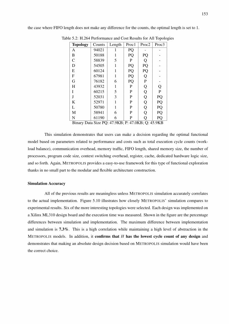
153
the case where FIFO length does not make any difference for the counts, the optimal length is set to 1.
Table 5.2: H.264 Performance and Cost Results for All Topologies
Topology Counts Length Proc1 Proc2 Proc3A 94021 1 PQ - -B 50188 1 PQ PQ -C 58839 5 P Q -D 54505 1 PQ PQ -E 60124 1 PQ PQ -F 67981 1 PQ Q -G 76182 6 PQ P -H 43932 1 P Q QI 60215 5 P Q PJ 52031 3 P Q PQK 52971 1 P Q PQL 50780 1 P Q PQM 58941 6 P Q PQN 61190 6 P Q PQBinary Data Size PQ: 47.9KB; P: 47.0KB; Q: 45.9KB
This simulation demonstrates that users can make a decision regarding the optimal functional
model based on parameters related to performance and costs such as total execution cycle counts (work-
load balance), communication overhead, memory traffic, FIFO length, shared memory size, the number of
processors, program code size, context switching overhead, register, cache, dedicated hardware logic size,
and so forth. Again, METROPOLIS provides a easy-to-use framework for this type of functional exploration
thanks in no small part to the modular and flexible architecture construction.
Simulation Accuracy
All of the previous results are meaningless unless METROPOLIS simulation accurately correlates
to the actual implementation. Figure 5.10 illustrates how closely METROPOLIS’ simulation compares to
experimental results. Six of the more interesting topologies were selected. Each design was implemented on
a Xilinx ML310 design board and the execution time was measured. Shown in the figure are the percentage
differences between simulation and implementation. The maximum difference between implementation
and simulation is 7.3%. This is a high correlation while maintaining a high level of abstraction in the
METROPOLIS models. In addition, it confirms that H has the lowest cycle count of any design and
demonstrates that making an absolute design decision based on METROPOLIS simulation would have been
the correct choice.
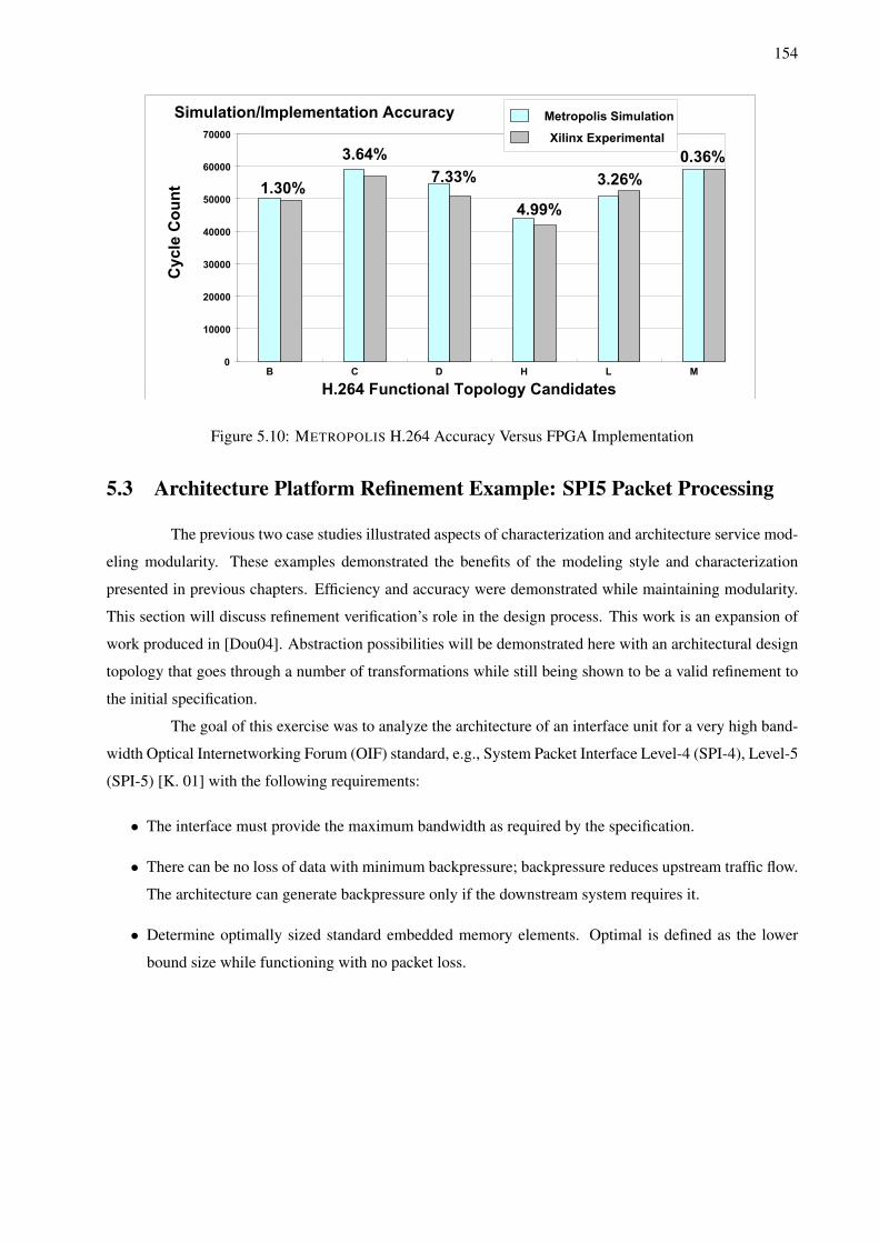
154
0
10000
20000
30000
40000
50000
60000
70000
B C D H L M
Metropolis Simulation
Xilinx Experimental
1.30%
3.64%
7.33%
4.99%
3.26%
0.36%C
yc
le C
ou
nt
H.264 Functional Topology Candidates
Simulation/Implementation Accuracy
Figure 5.10: METROPOLIS H.264 Accuracy Versus FPGA Implementation
5.3 Architecture Platform Refinement Example: SPI5 Packet Processing
The previous two case studies illustrated aspects of characterization and architecture service mod-
eling modularity. These examples demonstrated the benefits of the modeling style and characterization
presented in previous chapters. Efficiency and accuracy were demonstrated while maintaining modularity.
This section will discuss refinement verification’s role in the design process. This work is an expansion of
work produced in [Dou04]. Abstraction possibilities will be demonstrated here with an architectural design
topology that goes through a number of transformations while still being shown to be a valid refinement to
the initial specification.
The goal of this exercise was to analyze the architecture of an interface unit for a very high band-
width Optical Internetworking Forum (OIF) standard, e.g., System Packet Interface Level-4 (SPI-4), Level-5
(SPI-5) [K. 01] with the following requirements:
• The interface must provide the maximum bandwidth as required by the specification.
• There can be no loss of data with minimum backpressure; backpressure reduces upstream traffic flow.
The architecture can generate backpressure only if the downstream system requires it.
• Determine optimally sized standard embedded memory elements. Optimal is defined as the lower
bound size while functioning with no packet loss.
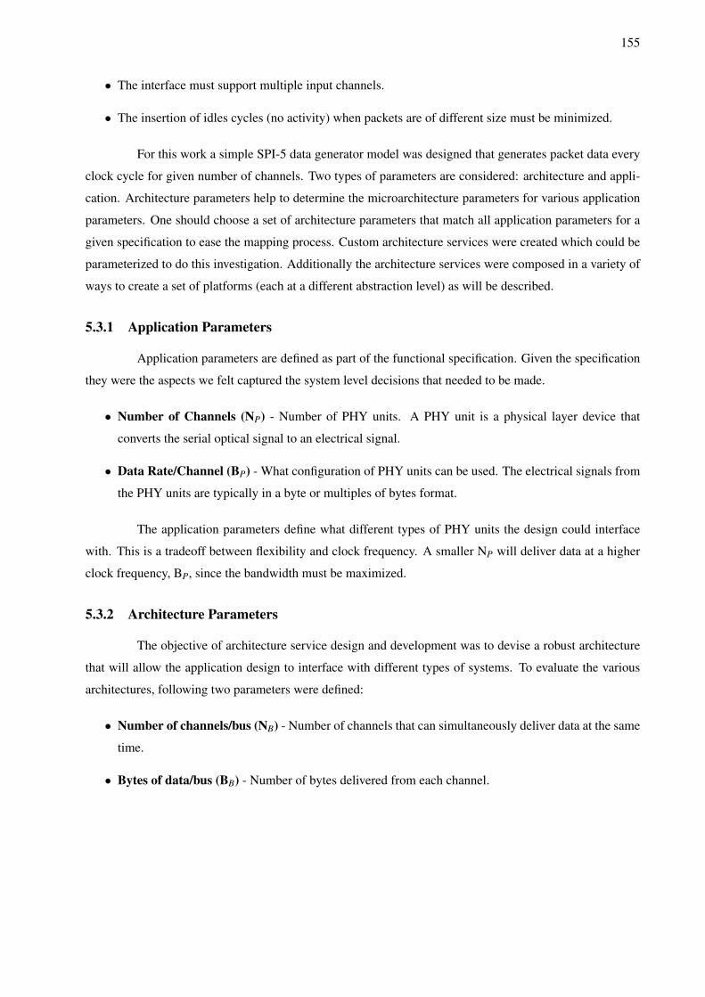
155
• The interface must support multiple input channels.
• The insertion of idles cycles (no activity) when packets are of different size must be minimized.
For this work a simple SPI-5 data generator model was designed that generates packet data every
clock cycle for given number of channels. Two types of parameters are considered: architecture and appli-
cation. Architecture parameters help to determine the microarchitecture parameters for various application
parameters. One should choose a set of architecture parameters that match all application parameters for a
given specification to ease the mapping process. Custom architecture services were created which could be
parameterized to do this investigation. Additionally the architecture services were composed in a variety of
ways to create a set of platforms (each at a different abstraction level) as will be described.
5.3.1 Application Parameters
Application parameters are defined as part of the functional specification. Given the specification
they were the aspects we felt captured the system level decisions that needed to be made.
• Number of Channels (NP) - Number of PHY units. A PHY unit is a physical layer device that
converts the serial optical signal to an electrical signal.
• Data Rate/Channel (BP) - What configuration of PHY units can be used. The electrical signals from
the PHY units are typically in a byte or multiples of bytes format.
The application parameters define what different types of PHY units the design could interface
with. This is a tradeoff between flexibility and clock frequency. A smaller NP will deliver data at a higher
clock frequency, BP, since the bandwidth must be maximized.
5.3.2 Architecture Parameters
The objective of architecture service design and development was to devise a robust architecture
that will allow the application design to interface with different types of systems. To evaluate the various
architectures, following two parameters were defined:
• Number of channels/bus (NB) - Number of channels that can simultaneously deliver data at the same
time.
• Bytes of data/bus (BB) - Number of bytes delivered from each channel.
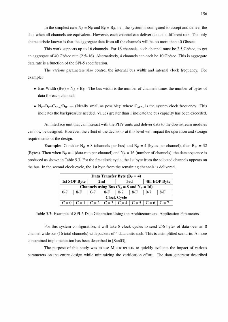
156
In the simplest case NP = NB and BP = BB, i.e., the system is configured to accept and deliver the
data when all channels are equivalent. However, each channel can deliver data at a different rate. The only
characteristic known is that the aggregate data from all the channels will be no more than 40 Gb/sec.
This work supports up to 16 channels. For 16 channels, each channel must be 2.5 Gb/sec, to get
an aggregate of 40 Gb/sec rate (2.5∗16). Alternatively, 4 channels can each be 10 Gb/sec. This is aggregate
data rate is a function of the SPI-5 specification.
The various parameters also control the internal bus width and internal clock frequency. For
example:
• Bus Width (BW ) = NB ∗ BB - The bus width is the number of channels times the number of bytes of
data for each channel.
• NP∗BP∗CSY S/BW → (Ideally small as possible); where CSY S, is the system clock frequency. This
indicates the backpressure needed. Values greater than 1 indicate the bus capacity has been exceeded.
An interface unit that can interact with the PHY units and deliver data to the downstream modules
can now be designed. However, the effect of the decisions at this level will impact the operation and storage
requirements of the design.
Example: Consider NB = 8 (channels per bus) and BB = 4 (bytes per channel), then BW = 32
(Bytes). Then when BP = 4 (data rate per channel) and NP = 16 (number of channels), the data sequence is
produced as shown in Table 5.3. For the first clock cycle, the 1st byte from the selected channels appears on
the bus. In the second clock cycle, the 1st byte from the remaining channels is delivered.
Data Transfer Byte (BP = 4)1st SOP Byte 2nd 3rd 4th EOP Byte
Channels using Bus (Nb = 8 and Np = 16)0-7 8-F 0-7 8-F 0-7 8-F 0-7 8-F
Clock CycleC = 0 C = 1 C = 2 C = 3 C = 4 C = 5 C = 6 C = 7
Table 5.3: Example of SPI-5 Data Generation Using the Architecture and Application Parameters
For this system configuration, it will take 8 clock cycles to send 256 bytes of data over an 8
channel wide bus (16 total channels) with packets of 4 data units each. This is a simplified scenario. A more
constrained implementation has been described in [San03].
The purpose of this study was to use METROPOLIS to quickly evaluate the impact of various
parameters on the entire design while minimizing the verification effort. The data generator described
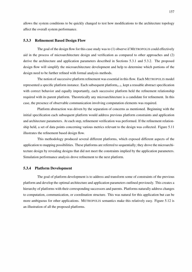
157
allows the system conditions to be quickly changed to test how modifications to the architecture topology
affect the overall system performance.
5.3.3 Refinement Based Design Flow
The goal of the design flow for this case study was to (1) observe if METROPOLIS could effectively
aid in the process of microarchitecture design and verification as compared to other approaches and (2)
derive the architecture and application parameters described in Sections 5.3.1 and 5.3.2. The proposed
design flow will simplify the microarchitecture development and help to determine which portions of the
design need to be further refined with formal analysis methods.
The notion of successive platform refinement was essential in this flow. Each METROPOLIS model
represented a specific platform instance. Each subsequent platformi+1, kept a reusable abstract specification
with correct behavior and equally importantly, each successive platform held the refinement relationship
required with its parent platform. Theoretically any microarchitecture is a candidate for refinement. In this
case, the presence of observable communication involving computation elements was required.
Platform abstraction was driven by the separation of concerns as mentioned. Beginning with the
initial specification each subsequent platform would address previous platform constraints and application
and architecture parameters. At each step, refinement verification was performed. If the refinement relation-
ship held, a set of data points concerning various metrics relevant to the design was collected. Figure 5.11
illustrates the refinement based design flow.
This methodology produced several different platforms, which exposed different aspects of the
application to mapping possibilities. These platforms are referred to sequentially; they drove the microarchi-
tecture design by revealing designs that did not meet the constraints implied by the application parameters.
Simulation performance analysis drove refinement to the next platform.
5.3.4 Platform Development
The goal of platform development is to address and transform some of constraints of the previous
platform and develop the optimal architecture and application parameters outlined previously. This creates a
hierarchy of platforms with their corresponding successors and parents. Platforms naturally address changes
to computation, communication, or coordination structure. This was natural for this application but can be
more ambiguous for other applications. METROPOLIS semantics make this relatively easy. Figure 5.12 is
an illustration of all the proposed platforms.
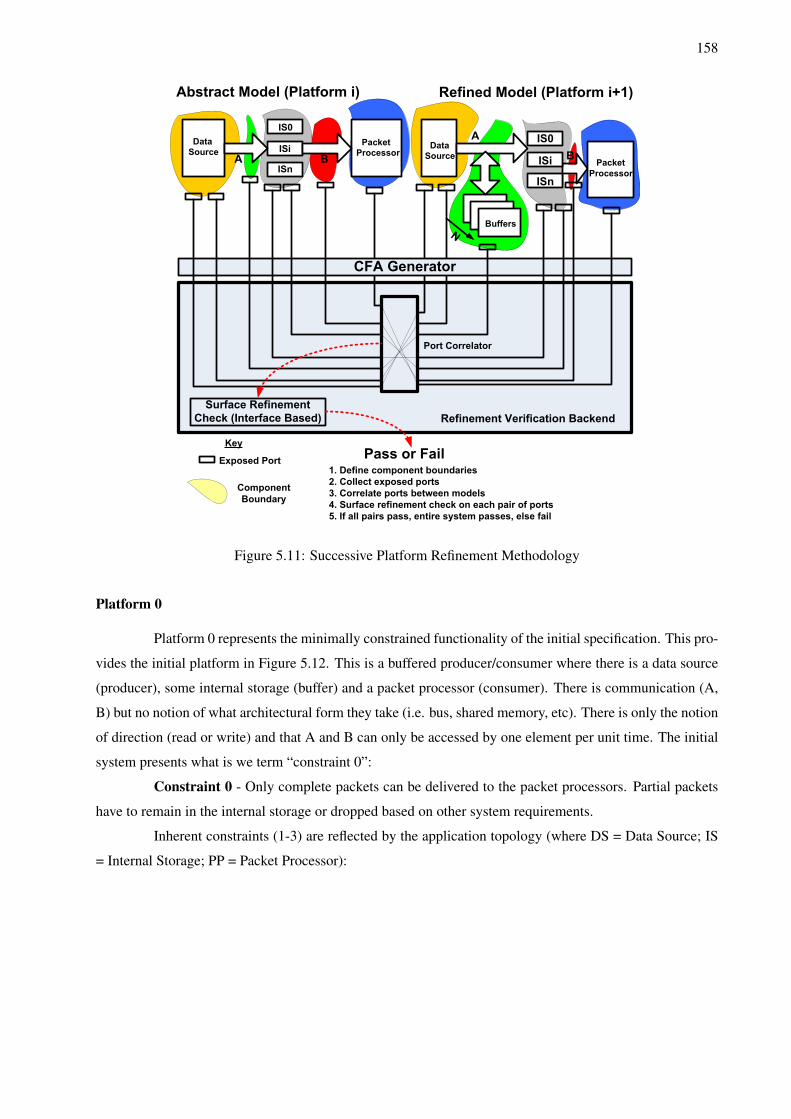
158
CFA Generator
Data
SourcePacket
Processor
IS0
ISn
ISiA B
Data
Source
A
Packet
Processor
BuffersN
IS0
ISn
ISi
Abstract Model (Platform i) Refined Model (Platform i+1)
Exposed Port
Component
Boundary
Key
Refinement Verification Backend
Port Correlator
Surface Refinement
Check (Interface Based)
Pass or Fail1. Define component boundaries
2. Collect exposed ports
3. Correlate ports between models
4. Surface refinement check on each pair of ports
5. If all pairs pass, entire system passes, else fail
B
Figure 5.11: Successive Platform Refinement Methodology
Platform 0
Platform 0 represents the minimally constrained functionality of the initial specification. This pro-
vides the initial platform in Figure 5.12. This is a buffered producer/consumer where there is a data source
(producer), some internal storage (buffer) and a packet processor (consumer). There is communication (A,
B) but no notion of what architectural form they take (i.e. bus, shared memory, etc). There is only the notion
of direction (read or write) and that A and B can only be accessed by one element per unit time. The initial
system presents what is we term “constraint 0”:
Constraint 0 - Only complete packets can be delivered to the packet processors. Partial packets
have to remain in the internal storage or dropped based on other system requirements.
Inherent constraints (1-3) are reflected by the application topology (where DS = Data Source; IS
= Internal Storage; PP = Packet Processor):
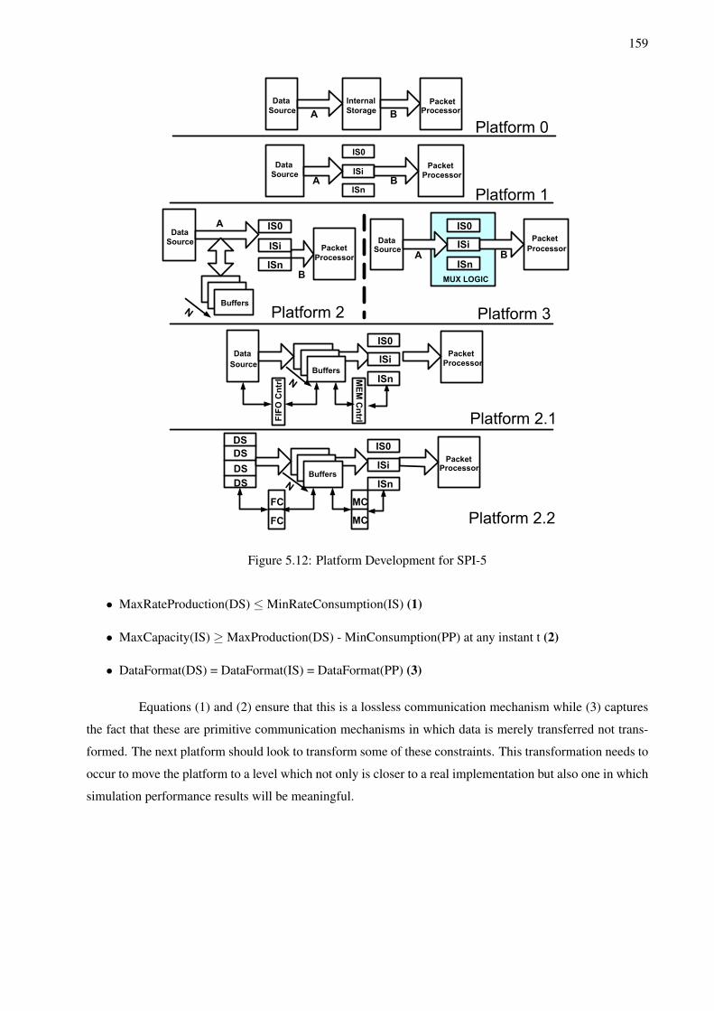
159
MUX LOGIC
Data
Source A
Internal
Storage B
PacketProcessor
Data
SourcePacket
Processor
IS0
ISn
ISiA B
DataSource
Packet
Processor
IS0
ISn
ISiA B
Data
Source
A
B
Packet
Processor
Buffers
Data
Source
Packet
ProcessorBuffers
N
DS
DS
DS
DS
PacketProcessor
Buffers
FC
FC
MC
MC
N
N
IS0
ISn
ISi
IS0
ISn
ISi
IS0
ISn
ISi
FIFO Cntrl M
EM Cntrl
Figure 5.12: Platform Development for SPI-5
• MaxRateProduction(DS) ≤ MinRateConsumption(IS) (1)
• MaxCapacity(IS) ≥ MaxProduction(DS) - MinConsumption(PP) at any instant t (2)
• DataFormat(DS) = DataFormat(IS) = DataFormat(PP) (3)
Equations (1) and (2) ensure that this is a lossless communication mechanism while (3) captures
the fact that these are primitive communication mechanisms in which data is merely transferred not trans-
formed. The next platform should look to transform some of these constraints. This transformation needs to
occur to move the platform to a level which not only is closer to a real implementation but also one in which
simulation performance results will be meaningful.
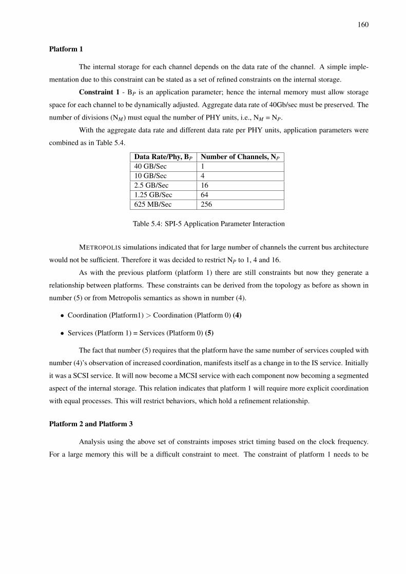
160
Platform 1
The internal storage for each channel depends on the data rate of the channel. A simple imple-
mentation due to this constraint can be stated as a set of refined constraints on the internal storage.
Constraint 1 - BP is an application parameter; hence the internal memory must allow storage
space for each channel to be dynamically adjusted. Aggregate data rate of 40Gb/sec must be preserved. The
number of divisions (NM) must equal the number of PHY units, i.e., NM = NP.
With the aggregate data rate and different data rate per PHY units, application parameters were
combined as in Table 5.4.
Data Rate/Phy, BP Number of Channels, NP
40 GB/Sec 110 GB/Sec 42.5 GB/Sec 161.25 GB/Sec 64625 MB/Sec 256
Table 5.4: SPI-5 Application Parameter Interaction
METROPOLIS simulations indicated that for large number of channels the current bus architecture
would not be sufficient. Therefore it was decided to restrict NP to 1, 4 and 16.
As with the previous platform (platform 1) there are still constraints but now they generate a
relationship between platforms. These constraints can be derived from the topology as before as shown in
number (5) or from Metropolis semantics as shown in number (4).
• Coordination (Platform1) > Coordination (Platform 0) (4)
• Services (Platform 1) = Services (Platform 0) (5)
The fact that number (5) requires that the platform have the same number of services coupled with
number (4)’s observation of increased coordination, manifests itself as a change in to the IS service. Initially
it was a SCSI service. It will now become a MCSI service with each component now becoming a segmented
aspect of the internal storage. This relation indicates that platform 1 will require more explicit coordination
with equal processes. This will restrict behaviors, which hold a refinement relationship.
Platform 2 and Platform 3
Analysis using the above set of constraints imposes strict timing based on the clock frequency.
For a large memory this will be a difficult constraint to meet. The constraint of platform 1 needs to be
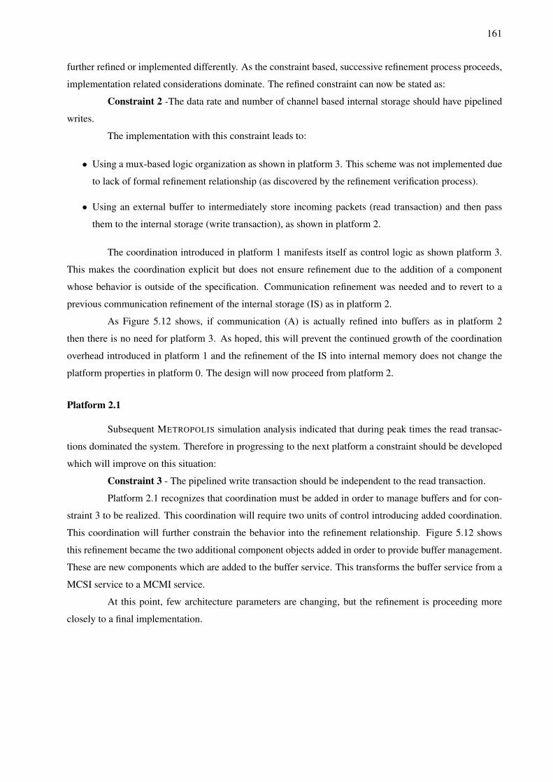
161
further refined or implemented differently. As the constraint based, successive refinement process proceeds,
implementation related considerations dominate. The refined constraint can now be stated as:
Constraint 2 -The data rate and number of channel based internal storage should have pipelined
writes.
The implementation with this constraint leads to:
• Using a mux-based logic organization as shown in platform 3. This scheme was not implemented due
to lack of formal refinement relationship (as discovered by the refinement verification process).
• Using an external buffer to intermediately store incoming packets (read transaction) and then pass
them to the internal storage (write transaction), as shown in platform 2.
The coordination introduced in platform 1 manifests itself as control logic as shown platform 3.
This makes the coordination explicit but does not ensure refinement due to the addition of a component
whose behavior is outside of the specification. Communication refinement was needed and to revert to a
previous communication refinement of the internal storage (IS) as in platform 2.
As Figure 5.12 shows, if communication (A) is actually refined into buffers as in platform 2
then there is no need for platform 3. As hoped, this will prevent the continued growth of the coordination
overhead introduced in platform 1 and the refinement of the IS into internal memory does not change the
platform properties in platform 0. The design will now proceed from platform 2.
Platform 2.1
Subsequent METROPOLIS simulation analysis indicated that during peak times the read transac-
tions dominated the system. Therefore in progressing to the next platform a constraint should be developed
which will improve on this situation:
Constraint 3 - The pipelined write transaction should be independent to the read transaction.
Platform 2.1 recognizes that coordination must be added in order to manage buffers and for con-
straint 3 to be realized. This coordination will require two units of control introducing added coordination.
This coordination will further constrain the behavior into the refinement relationship. Figure 5.12 shows
this refinement became the two additional component objects added in order to provide buffer management.
These are new components which are added to the buffer service. This transforms the buffer service from a
MCSI service to a MCMI service.
At this point, few architecture parameters are changing, but the refinement is proceeding more
closely to a final implementation.
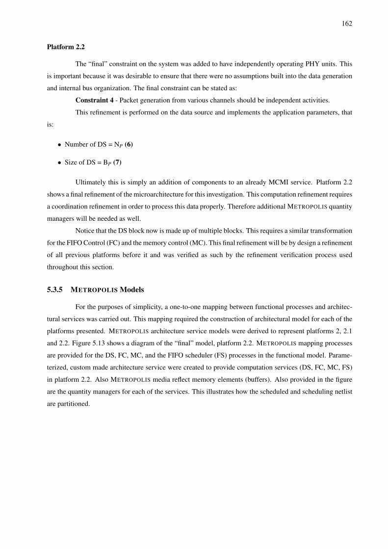
162
Platform 2.2
The “final” constraint on the system was added to have independently operating PHY units. This
is important because it was desirable to ensure that there were no assumptions built into the data generation
and internal bus organization. The final constraint can be stated as:
Constraint 4 - Packet generation from various channels should be independent activities.
This refinement is performed on the data source and implements the application parameters, that
is:
• Number of DS = NP (6)
• Size of DS = BP (7)
Ultimately this is simply an addition of components to an already MCMI service. Platform 2.2
shows a final refinement of the microarchitecture for this investigation. This computation refinement requires
a coordination refinement in order to process this data properly. Therefore additional METROPOLIS quantity
managers will be needed as well.
Notice that the DS block now is made up of multiple blocks. This requires a similar transformation
for the FIFO Control (FC) and the memory control (MC). This final refinement will be by design a refinement
of all previous platforms before it and was verified as such by the refinement verification process used
throughout this section.
5.3.5 METROPOLIS Models
For the purposes of simplicity, a one-to-one mapping between functional processes and architec-
tural services was carried out. This mapping required the construction of architectural model for each of the
platforms presented. METROPOLIS architecture service models were derived to represent platforms 2, 2.1
and 2.2. Figure 5.13 shows a diagram of the “final” model, platform 2.2. METROPOLIS mapping processes
are provided for the DS, FC, MC, and the FIFO scheduler (FS) processes in the functional model. Parame-
terized, custom made architecture service were created to provide computation services (DS, FC, MC, FS)
in platform 2.2. Also METROPOLIS media reflect memory elements (buffers). Also provided in the figure
are the quantity managers for each of the services. This illustrates how the scheduled and scheduling netlist
are partitioned.
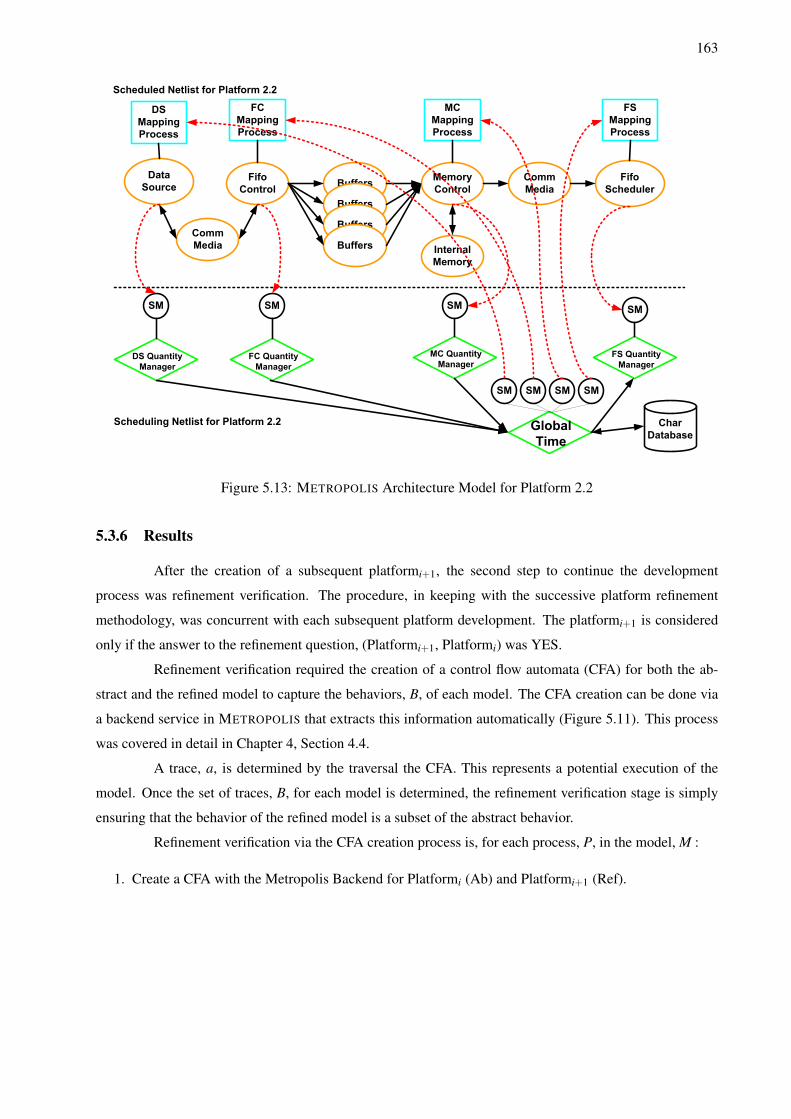
163
DS
Mapping
Process
FC
Mapping
Process
MC
Mapping
Process
FS
Mapping
Process
Comm
Media
Comm
MediaBuffers
Fifo
Control
Fifo
Scheduler
Data
SourceMemory
Control
Buffers
Buffers
Buffers Internal
Memory
Scheduled Netlist for Platform 2.2
Scheduling Netlist for Platform 2.2
SM SM SM SM
Global
Time
SM SM SM SM
Char
Database
DS Quantity
Manager
FS Quantity
ManagerFC Quantity
Manager
MC Quantity
Manager
Figure 5.13: METROPOLIS Architecture Model for Platform 2.2
5.3.6 Results
After the creation of a subsequent platformi+1, the second step to continue the development
process was refinement verification. The procedure, in keeping with the successive platform refinement
methodology, was concurrent with each subsequent platform development. The platformi+1 is considered
only if the answer to the refinement question, (Platformi+1, Platformi) was YES.
Refinement verification required the creation of a control flow automata (CFA) for both the ab-
stract and the refined model to capture the behaviors, B, of each model. The CFA creation can be done via
a backend service in METROPOLIS that extracts this information automatically (Figure 5.11). This process
was covered in detail in Chapter 4, Section 4.4.
A trace, a, is determined by the traversal the CFA. This represents a potential execution of the
model. Once the set of traces, B, for each model is determined, the refinement verification stage is simply
ensuring that the behavior of the refined model is a subset of the abstract behavior.
Refinement verification via the CFA creation process is, for each process, P, in the model, M :
1. Create a CFA with the Metropolis Backend for Platformi (Ab) and Platformi+1 (Ref).
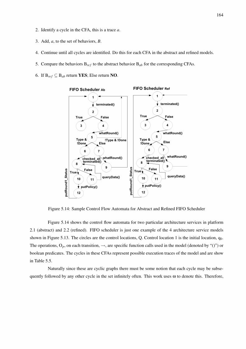
164
2. Identify a cycle in the CFA, this is a trace a.
3. Add, a, to the set of behaviors, B.
4. Continue until all cycles are identified. Do this for each CFA in the abstract and refined models.
5. Compare the behaviors Bre f to the abstract behavior Bab for the corresponding CFAs.
6. If Bre f ⊆ Bab return YES; Else return NO.
1
3
2
4
5
6 7
89
10 11
12
terminated()
True False
whatRound()
Type &
!Done Else
whatRound()checked_allterminated()
TrueFalse
FIFO Scheduler Ref
queryData()
putPolicy()
pu
tRo
un
d1
_S
tatu
s
FIFO Scheduler Ab
1
3
2
4
5
6 7
89
10 11
12
terminated()
True False
whatRound()
Type &
!Done Else
whatRound()checked_allterminated()
TrueFalse
queryData()
putPolicy()
pu
tRo
un
d1
_S
tatu
s
!Type & !Done
Figure 5.14: Sample Control Flow Automata for Abstract and Refined FIFO Scheduler
Figure 5.14 shows the control flow automata for two particular architecture services in platform
2.1 (abstract) and 2.2 (refined). FIFO scheduler is just one example of the 4 architecture service models
shown in Figure 5.13. The circles are the control locations, Q. Control location 1 is the initial location, q0.
The operations, Op, on each transition, →, are specific function calls used in the model (denoted by “()”) or
boolean predicates. The cycles in these CFAs represent possible execution traces of the model and are show
in Table 5.5.
Naturally since these are cyclic graphs there must be some notion that each cycle may be subse-
quently followed by any other cycle in the set infinitely often. This work uses ω to denote this. Therefore,
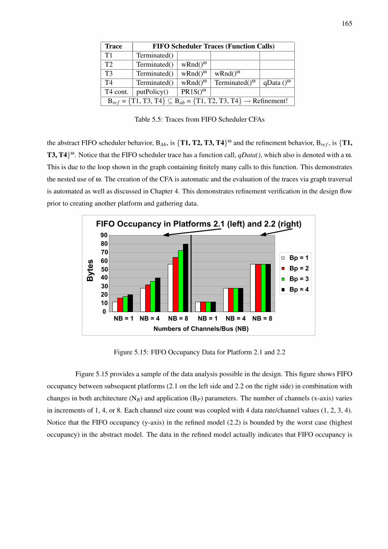
165
Trace FIFO Scheduler Traces (Function Calls)T1 Terminated()T2 Terminated() wRnd()ω
T3 Terminated() wRnd()ω wRnd()ω
T4 Terminated() wRnd()ω Terminated()ω qData ()ω
T4 cont. putPolicy() PR1S()ω
Bre f = {T1, T3, T4} ⊆ Bab = {T1, T2, T3, T4} → Refinement!
Table 5.5: Traces from FIFO Scheduler CFAs
the abstract FIFO scheduler behavior, BAb, is {T1, T2, T3, T4}ω and the refinement behavior, Bre f , is {T1,
T3, T4}ω. Notice that the FIFO scheduler trace has a function call, qData(), which also is denoted with a ω.
This is due to the loop shown in the graph containing finitely many calls to this function. This demonstrates
the nested use of ω. The creation of the CFA is automatic and the evaluation of the traces via graph traversal
is automated as well as discussed in Chapter 4. This demonstrates refinement verification in the design flow
prior to creating another platform and gathering data.
FIFO Occupancy in Platforms 2.1 (left) and 2.2 (right)
0
10
20
30
40
50
60
70
80
90
NB = 1 NB = 4 NB = 8 NB = 1 NB = 4 NB = 8
Numbers of Channels/Bus (NB)
Bytes
Bp = 1
Bp = 2
Bp = 3
Bp = 4
Figure 5.15: FIFO Occupancy Data for Platform 2.1 and 2.2
Figure 5.15 provides a sample of the data analysis possible in the design. This figure shows FIFO
occupancy between subsequent platforms (2.1 on the left side and 2.2 on the right side) in combination with
changes in both architecture (NB) and application (BP) parameters. The number of channels (x-axis) varies
in increments of 1, 4, or 8. Each channel size count was coupled with 4 data rate/channel values (1, 2, 3, 4).
Notice that the FIFO occupancy (y-axis) in the refined model (2.2) is bounded by the worst case (highest
occupancy) in the abstract model. The data in the refined model actually indicates that FIFO occupancy is
166
unaffected by BP and that for all 4 settings the occupancy is the same as BP = 1 in the abstract model. This
type of data analysis will drive the platform development in the future and demonstrates the usefulness of
design exploration.
5.4 Communication Subsystem Refinement Example: FLEET Communica-
tion Structure
This section and final case study will demonstrate another refinement technique discussed previ-
ously, “depth” refinement. The purpose of the example presented here is to explore how various communi-
cation structures can be replaced in a design without changing the surrounding components. These changes
are verified before the substitution using the techniques discussed in Chapter 4, Section 4.5. This substitu-
tion then becomes “correct-by-construction”. This differs from the example shown in Section 5.3 because
the topologies of the architecture models in this section remain the same but the operations internally in
the components are changed. This case study example is performed on a model of the FLEET architecture
(described in Section 2.5). Specifically it is a manipulation of its communication structure where there exists
a great deal of underspecification.
5.4.1 Communication Library
The first step in developing a refinement framework is the creation of library of communication
services. These services which are created first in METROPOLIS or SystemC are then transformed into LTS
and have a corresponding architecture service interface. E for each LTS system S corresponds to events in the
architecture service model, EE . Events have been described in the context of the METROPOLIS environment
previously. The concept of event synchronization can exist as well in a SystemC model. This section will
detail those architecture services in terms of their LTS representations. In all descriptions, the when an event
is described as “emitted” it refers to the generation of a visible event, EEV .
• Abstract Buffer (AB): An abstract buffer is defined to buffer data. It contains states that are repre-
sentative of an nplace buffer: Q = {empty, not empty, full}. Qo = empty, and upon receiving a write
event, it will transition to not empty while emitting an event to signal a successful write. Similarly a
transition occurs from not empty to full. Read events from a consumer cause transitions to empty and
not empty states. This process also emits an event signaling a successful read. Events are not emitted
when in the full or empty states for write and read request respectively. This buffer provides blocking
semantics.
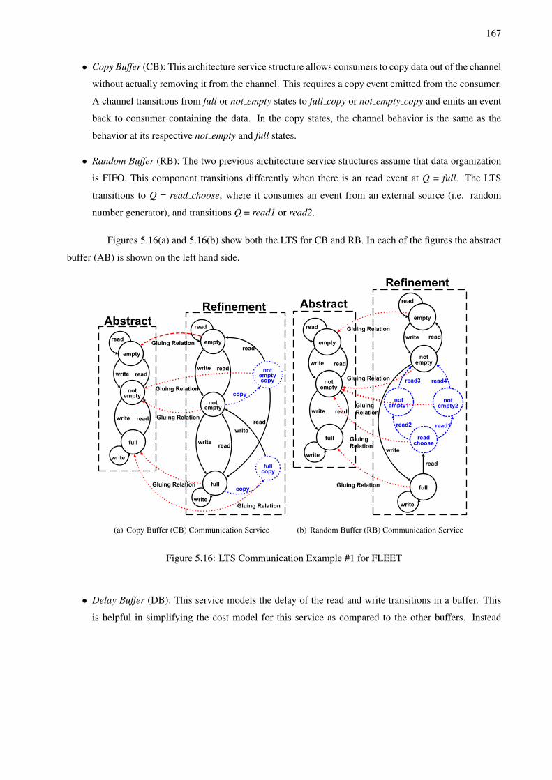
167
• Copy Buffer (CB): This architecture service structure allows consumers to copy data out of the channel
without actually removing it from the channel. This requires a copy event emitted from the consumer.
A channel transitions from full or not empty states to full copy or not empty copy and emits an event
back to consumer containing the data. In the copy states, the channel behavior is the same as the
behavior at its respective not empty and full states.
• Random Buffer (RB): The two previous architecture service structures assume that data organization
is FIFO. This component transitions differently when there is an read event at Q = full. The LTS
transitions to Q = read choose, where it consumes an event from an external source (i.e. random
number generator), and transitions Q = read1 or read2.
Figures 5.16(a) and 5.16(b) show both the LTS for CB and RB. In each of the figures the abstract
buffer (AB) is shown on the left hand side.
empty
notempty
full
write
write
write
read
read
read
empty
notempty
full
write
write
write
read
read
read
notemptycopy
read
read
fullcopy
copy
copy
write
Gluing Relation
Gluing Relation
Gluing Relation
Gluing Relation
Gluing Relation
(a) Copy Buffer (CB) Communication Service
empty
notempty
full
write
write
write
read
read
empty
notempty
full
write
write
write
read
read
read
read
readchoose
notempty1
notempty2
read1read2
read3 read4
Gluing Relation
Gluing Relation
Gluing Relation
Gluing
Relation
Gluing
Relation
(b) Random Buffer (RB) Communication Service
Figure 5.16: LTS Communication Example #1 for FLEET
• Delay Buffer (DB): This service models the delay of the read and write transitions in a buffer. This
is helpful in simplifying the cost model for this service as compared to the other buffers. Instead
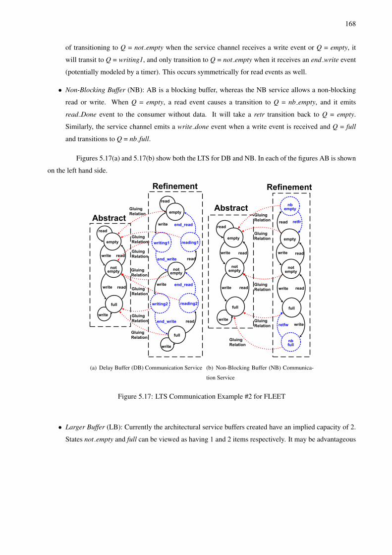
168
of transitioning to Q = not empty when the service channel receives a write event or Q = empty, it
will transit to Q = writing1, and only transition to Q = not empty when it receives an end write event
(potentially modeled by a timer). This occurs symmetrically for read events as well.
• Non-Blocking Buffer (NB): AB is a blocking buffer, whereas the NB service allows a non-blocking
read or write. When Q = empty, a read event causes a transition to Q = nb empty, and it emits
read Done event to the consumer without data. It will take a retr transition back to Q = empty.
Similarly, the service channel emits a write done event when a write event is received and Q = full
and transitions to Q = nb full.
Figures 5.17(a) and 5.17(b) show both the LTS for DB and NB. In each of the figures AB is shown
on the left hand side.
empty
notempty
full
write
write
write
read
read
empty
notempty
full
write
write
write
read
read
read
read
writing1 reading1
writing2 reading2
end_read
end_write
end_read
end_write
Gluing
Relation
Gluing
Relation
Gluing
Relation
Gluing
Relation
Gluing
Relation
Gluing
Relation
Gluing
Relation
(a) Delay Buffer (DB) Communication Service
empty
notempty
full
write
write
write
read
read
empty
notempty
full
write
write
read
read
read
read
nbempty
retfr
nbfull
retfw write
Gluing
Relation
Gluing
Relation
Gluing
Relation
Gluing
Relation
Gluing
Relation
(b) Non-Blocking Buffer (NB) Communica-
tion Service
Figure 5.17: LTS Communication Example #2 for FLEET
• Larger Buffer (LB): Currently the architectural service buffers created have an implied capacity of 2.
States not empty and full can be viewed as having 1 and 2 items respectively. It may be advantageous
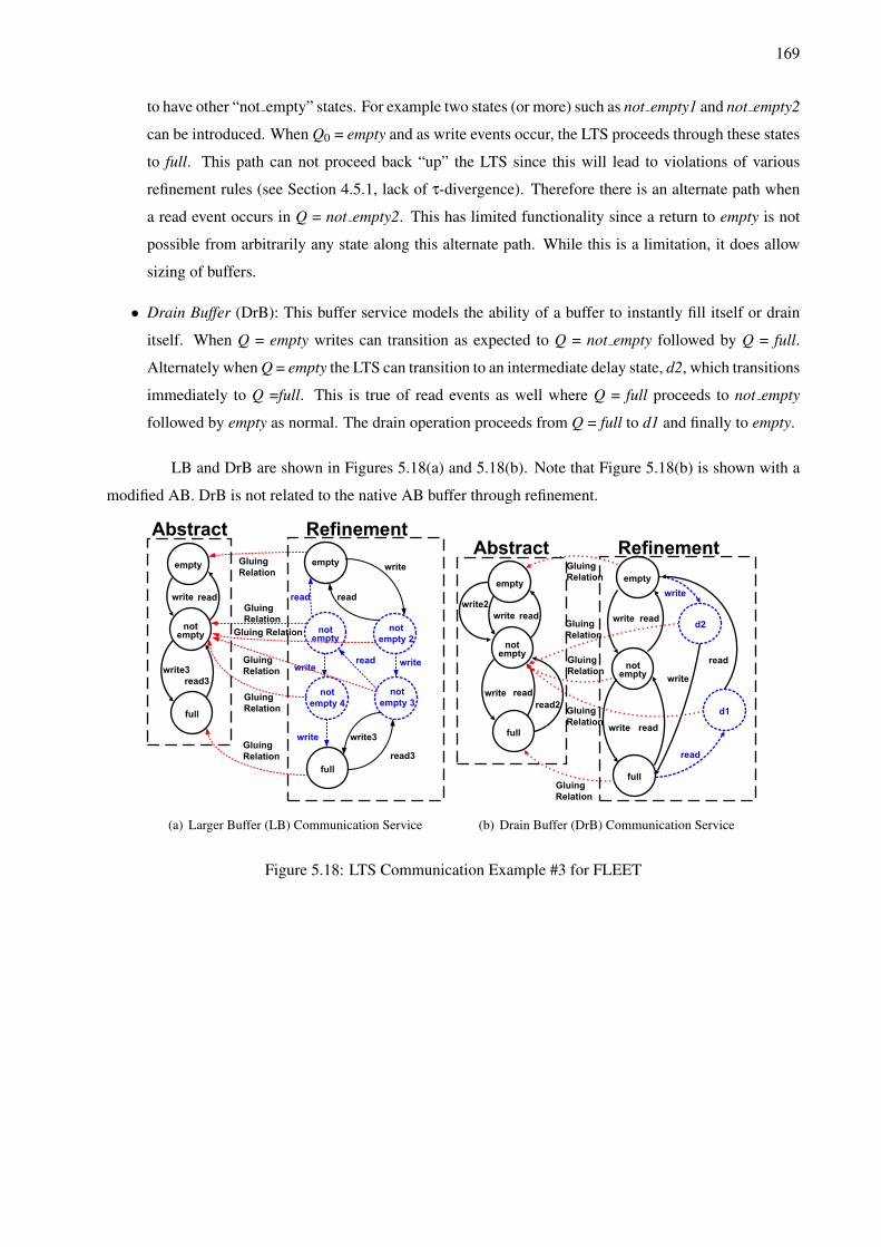
169
to have other “not empty” states. For example two states (or more) such as not empty1 and not empty2
can be introduced. When Q0 = empty and as write events occur, the LTS proceeds through these states
to full. This path can not proceed back “up” the LTS since this will lead to violations of various
refinement rules (see Section 4.5.1, lack of τ-divergence). Therefore there is an alternate path when
a read event occurs in Q = not empty2. This has limited functionality since a return to empty is not
possible from arbitrarily any state along this alternate path. While this is a limitation, it does allow
sizing of buffers.
• Drain Buffer (DrB): This buffer service models the ability of a buffer to instantly fill itself or drain
itself. When Q = empty writes can transition as expected to Q = not empty followed by Q = full.
Alternately when Q = empty the LTS can transition to an intermediate delay state, d2, which transitions
immediately to Q =full. This is true of read events as well where Q = full proceeds to not empty
followed by empty as normal. The drain operation proceeds from Q = full to d1 and finally to empty.
LB and DrB are shown in Figures 5.18(a) and 5.18(b). Note that Figure 5.18(b) is shown with a
modified AB. DrB is not related to the native AB buffer through refinement.
empty
notempty
full
write
write3
read
read3
empty
notempty
full
not
empty 3
not
empty 2
read3
write
read
write
write
write
read
read
Gluing
Relation
Gluing
Relation
Gluing
Relation
Gluing
Relation
Gluing
Relation
not
empty 4
write3
Gluing Relation
(a) Larger Buffer (LB) Communication Service
empty
notempty
full
write
write
read
read
empty
notempty
full
d1
d2
write2
read2
readwrite
readwrite
write
write
read
read
Gluing
Relation
Gluing
Relation
Gluing
Relation
Gluing
Relation
Gluing
Relation
(b) Drain Buffer (DrB) Communication Service
Figure 5.18: LTS Communication Example #3 for FLEET
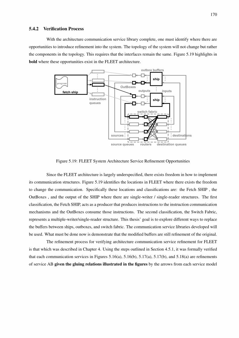
170
5.4.2 Verification Process
With the architecture communication service library complete, one must identify where there are
opportunities to introduce refinement into the system. The topology of the system will not change but rather
the components in the topology. This requires that the interfaces remain the same. Figure 5.19 highlights in
bold where these opportunities exist in the FLEET architecture.
fetch ship inputs
ship
ship
program
instruction
queues
sources
source queues destination queues
destinations
switch fabric
routers
outbox buffers
OutBoxes
outputs
Figure 5.19: FLEET System Architecture Service Refinement Opportunities
Since the FLEET architecture is largely underspecified, there exists freedom in how to implement
its communication structures. Figure 5.19 identifies the locations in FLEET where there exists the freedom
to change the communication. Specifically these locations and classifications are: the Fetch SHIP , the
OutBoxes , and the output of the SHIP where there are single-writer / single-reader structures. The first
classification, the Fetch SHIP, acts as a producer that produces instructions to the instruction communication
mechanisms and the OutBoxes consume those instructions. The second classification, the Switch Fabric,
represents a multiple-writer/single-reader structure. This thesis’ goal is to explore different ways to replace
the buffers between ships, outboxes, and switch fabric. The communication service libraries developed will
be used. What must be done now is demonstrate that the modified buffers are still refinement of the original.
The refinement process for verifying architecture communication service refinement for FLEET
is that which was described in Chapter 4. Using the steps outlined in Section 4.5.1, it was formally verified
that each communication services in Figures 5.16(a), 5.16(b), 5.17(a), 5.17(b), and 5.18(a) are refinements
of service AB given the gluing relations illustrated in the figures by the arrows from each service model
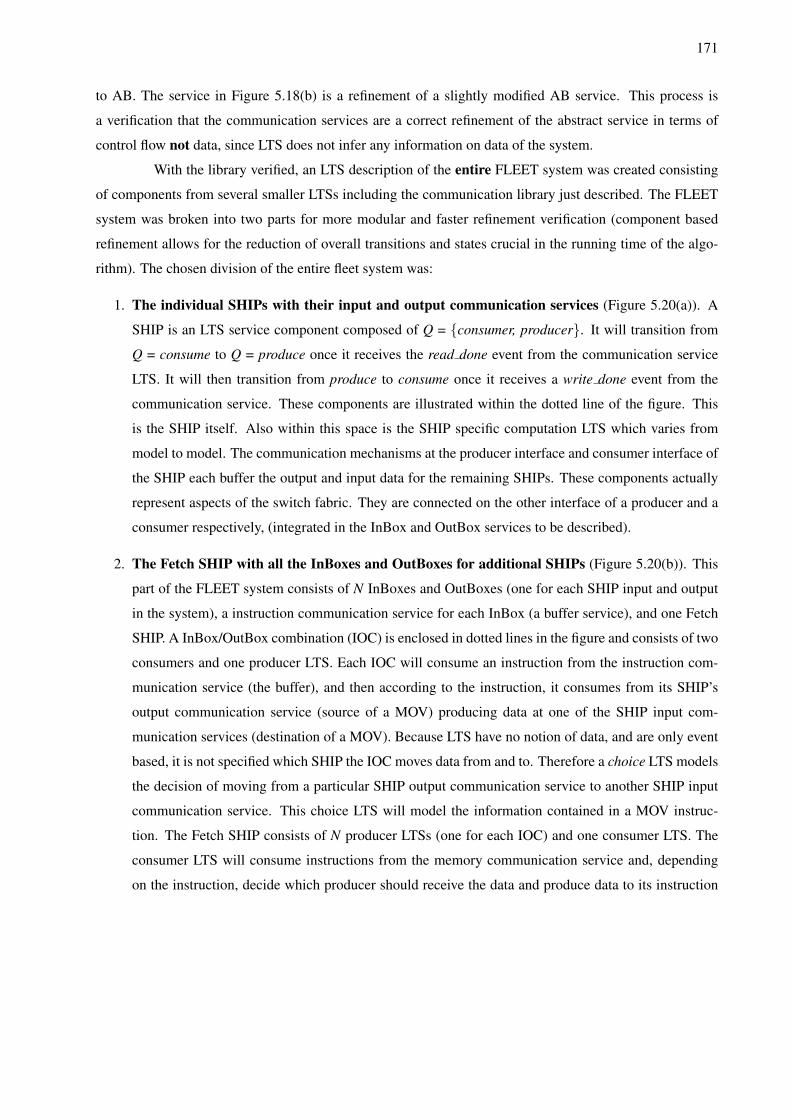
171
to AB. The service in Figure 5.18(b) is a refinement of a slightly modified AB service. This process is
a verification that the communication services are a correct refinement of the abstract service in terms of
control flow not data, since LTS does not infer any information on data of the system.
With the library verified, an LTS description of the entire FLEET system was created consisting
of components from several smaller LTSs including the communication library just described. The FLEET
system was broken into two parts for more modular and faster refinement verification (component based
refinement allows for the reduction of overall transitions and states crucial in the running time of the algo-
rithm). The chosen division of the entire fleet system was:
1. The individual SHIPs with their input and output communication services (Figure 5.20(a)). A
SHIP is an LTS service component composed of Q = {consumer, producer}. It will transition from
Q = consume to Q = produce once it receives the read done event from the communication service
LTS. It will then transition from produce to consume once it receives a write done event from the
communication service. These components are illustrated within the dotted line of the figure. This
is the SHIP itself. Also within this space is the SHIP specific computation LTS which varies from
model to model. The communication mechanisms at the producer interface and consumer interface of
the SHIP each buffer the output and input data for the remaining SHIPs. These components actually
represent aspects of the switch fabric. They are connected on the other interface of a producer and a
consumer respectively, (integrated in the InBox and OutBox services to be described).
2. The Fetch SHIP with all the InBoxes and OutBoxes for additional SHIPs (Figure 5.20(b)). This
part of the FLEET system consists of N InBoxes and OutBoxes (one for each SHIP input and output
in the system), a instruction communication service for each InBox (a buffer service), and one Fetch
SHIP. A InBox/OutBox combination (IOC) is enclosed in dotted lines in the figure and consists of two
consumers and one producer LTS. Each IOC will consume an instruction from the instruction com-
munication service (the buffer), and then according to the instruction, it consumes from its SHIP’s
output communication service (source of a MOV) producing data at one of the SHIP input com-
munication services (destination of a MOV). Because LTS have no notion of data, and are only event
based, it is not specified which SHIP the IOC moves data from and to. Therefore a choice LTS models
the decision of moving from a particular SHIP output communication service to another SHIP input
communication service. This choice LTS will model the information contained in a MOV instruc-
tion. The Fetch SHIP consists of N producer LTSs (one for each IOC) and one consumer LTS. The
consumer LTS will consume instructions from the memory communication service and, depending
on the instruction, decide which producer should receive the data and produce data to its instruction
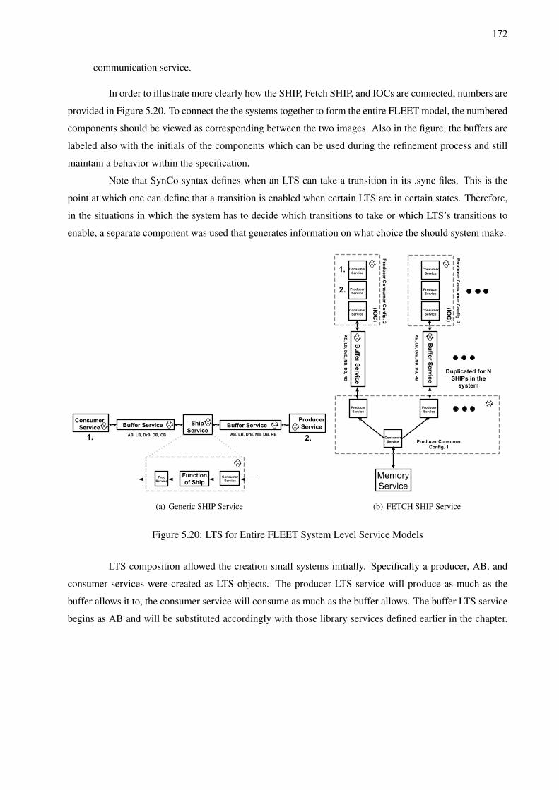
172
communication service.
In order to illustrate more clearly how the SHIP, Fetch SHIP, and IOCs are connected, numbers are
provided in Figure 5.20. To connect the the systems together to form the entire FLEET model, the numbered
components should be viewed as corresponding between the two images. Also in the figure, the buffers are
labeled also with the initials of the components which can be used during the refinement process and still
maintain a behavior within the specification.
Note that SynCo syntax defines when an LTS can take a transition in its .sync files. This is the
point at which one can define that a transition is enabled when certain LTS are in certain states. Therefore,
in the situations in which the system has to decide which transitions to take or which LTS’s transitions to
enable, a separate component was used that generates information on what choice the should system make.
Consumer
Service Buffer Service Ship
ServiceBuffer Service
Producer
Service
Prod
Service
Consumer
Service
Function
of Ship
AB, LB, DrB, DB, CB AB, LB, DrB, NB, DB, RB
(a) Generic SHIP Service
Consumer
Service
Buffer Service
Buffer Service
AB, LB, DrB, NB, DB, RB
AB, LB, DrB, NB, DB, RB
Consumer
Service
Consumer
Service
Consumer
Service
Consumer
Service
Producer
Service
Producer
Service
Producer
Service
Producer
Service
Producer Consumer
Config. 1
Producer Consumer Config. 2
Producer Consumer Config. 2
Duplicated for N
SHIPs in the
system
(IOC)
(IOC)
(b) FETCH SHIP Service
Figure 5.20: LTS for Entire FLEET System Level Service Models
LTS composition allowed the creation small systems initially. Specifically a producer, AB, and
consumer services were created as LTS objects. The producer LTS service will produce as much as the
buffer allows it to, the consumer service will consume as much as the buffer allows. The buffer LTS service
begins as AB and will be substituted accordingly with those library services defined earlier in the chapter.
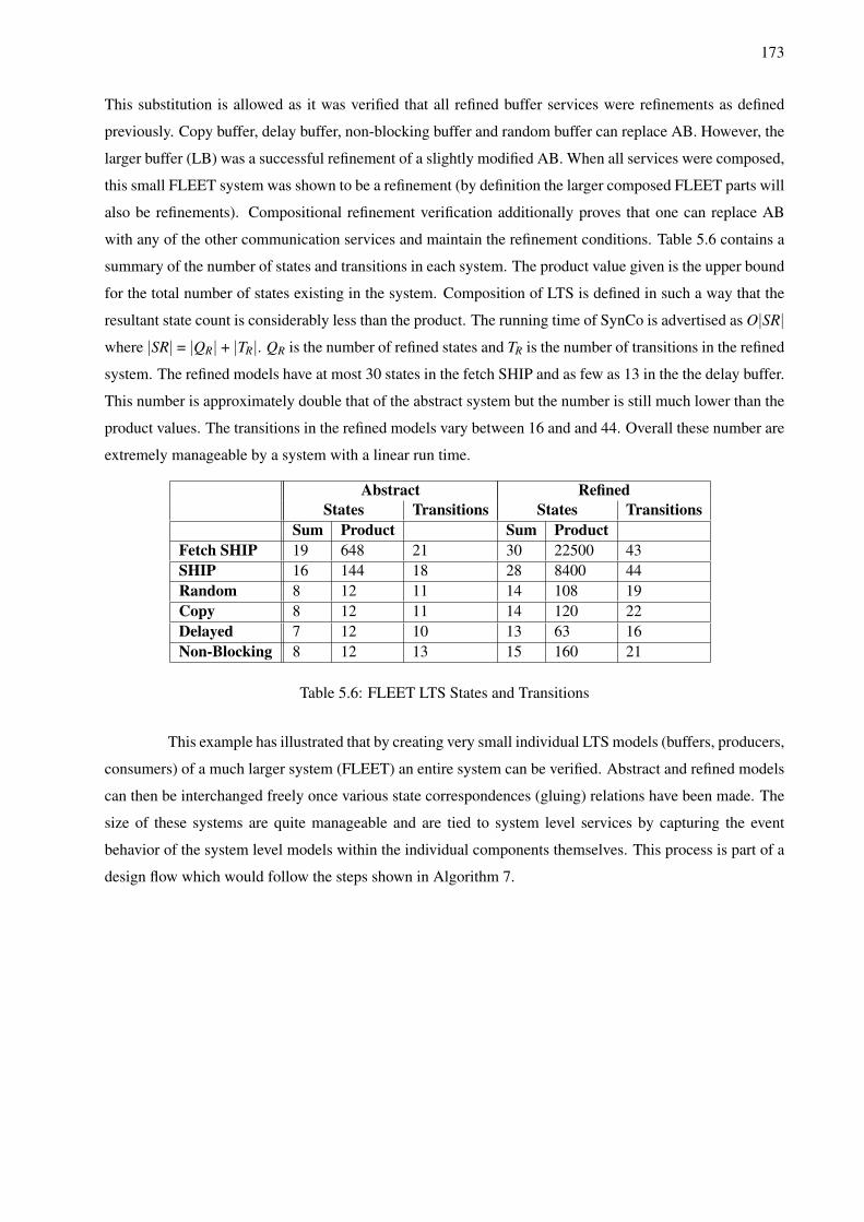
173
This substitution is allowed as it was verified that all refined buffer services were refinements as defined
previously. Copy buffer, delay buffer, non-blocking buffer and random buffer can replace AB. However, the
larger buffer (LB) was a successful refinement of a slightly modified AB. When all services were composed,
this small FLEET system was shown to be a refinement (by definition the larger composed FLEET parts will
also be refinements). Compositional refinement verification additionally proves that one can replace AB
with any of the other communication services and maintain the refinement conditions. Table 5.6 contains a
summary of the number of states and transitions in each system. The product value given is the upper bound
for the total number of states existing in the system. Composition of LTS is defined in such a way that the
resultant state count is considerably less than the product. The running time of SynCo is advertised as O|SR|where |SR| = |QR| + |TR|. QR is the number of refined states and TR is the number of transitions in the refined
system. The refined models have at most 30 states in the fetch SHIP and as few as 13 in the the delay buffer.
This number is approximately double that of the abstract system but the number is still much lower than the
product values. The transitions in the refined models vary between 16 and and 44. Overall these number are
extremely manageable by a system with a linear run time.
Abstract RefinedStates Transitions States Transitions
Sum Product Sum ProductFetch SHIP 19 648 21 30 22500 43SHIP 16 144 18 28 8400 44Random 8 12 11 14 108 19Copy 8 12 11 14 120 22Delayed 7 12 10 13 63 16Non-Blocking 8 12 13 15 160 21
Table 5.6: FLEET LTS States and Transitions
This example has illustrated that by creating very small individual LTS models (buffers, producers,
consumers) of a much larger system (FLEET) an entire system can be verified. Abstract and refined models
can then be interchanged freely once various state correspondences (gluing) relations have been made. The
size of these systems are quite manageable and are tied to system level services by capturing the event
behavior of the system level models within the individual components themselves. This process is part of a
design flow which would follow the steps shown in Algorithm 7.
174
Chapter 6
Conclusions and Contributions
“A conclusion is the place where you got tired thinking.” - Martin Henry Fischer
This thesis began with the proposition that ESL adoption was important for the EDA commu-
nity’s growth and for the continued viability of embedded electronic system design. ESL’s transition into
mainstream adoption would require that the design of system level architecture services be modular and
abstract while maintaining accuracy and efficiency. The “methodology gap” had to be crossed. This set of
requirements lead to the abandonment of a naıve design flow and to the adoption of a proposed design flow
which encompasses the following concepts:
• The introduction of “architecture services” as a means to implement behavior captured by a functional
description. Services provide interfaces which can be used to implement functionality. Additionally
services have costs associated with their usage.
• Transaction level, preemptable architecture services of parameterizable programmable platforms.
These specifically included METROPOLIS models of Xilinx’s Virtex II architecture and the FLEET
architecture. This construction allows a large design space exploration process with only one set of
library services.
• Automatic extraction of programmable system descriptions for synthesis. An architecture structure
extraction process creates the topology as a Microprocessor Hardware Specification (MHS) file for
Xilinx tool flows directly. This automation removes error prone manual techniques.
• Characterization flow for programmable platforms to be used during system simulation. This charac-
terization is captured in a METROPOLIS object located in the scheduling netlist which allows for zero

175
overhead, run-time annotation of events. This process allows for incremental addition of models as
well as being completely scalable and portable.
• Four refinement techniques (Vertical, Horizontal, Surface, Depth) based on three refinement verifica-
tion concepts (Event Based, Interface Based, Compositional Component Based) were illustrated for
unique refinement activities needed during the design space exploration process.
The contributions of this thesis were summarized in Table 1.6 in Chapter 1. The primary contri-
bution is the way in which programmable tool flows and devices were leveraged to explore a large design
space more accurately then previous approaches while using formal refinement techniques to proceed to-
ward implementations. While this flow can be extended to static architecture platforms, its strengths are
severely hindered by doing so.
Chapter 5 brought these techniques together with a set of four case studies (MJPEG encoding,
H.264 Deblocking Filter, SPI-5 packet processing, and FLEET communication subsystems) which demon-
strated the viability of various aspects of the proposed design flow. The summary of results could best be
stated by saying the property of design fidelity was maintained in all case studies and the infrastructure and
design techniques to ensure this fidelity did not reduce the efficiency of the design as compared to more
traditional methods.
This chapter will serve as a reflection on the successes and failures of the work presented throughout this
thesis as well as provide future directions upon which the work could be expanded on or improved.
6.0.3 Chapter Organization
This chapter is broken into two parts. The first part primarily summarizes the benefits (Section
6.1) and disadvantages (Section 6.2) of the design flow proposed throughout throughout this thesis. The
second part is a discussion of a future work (Section 6.3) in the areas of integrating all the techniques more
closely, formalizing them so that stronger claims can be made regarding the design process, and finally areas
for expansion.
6.1 Benefits
This section discusses three benefits in this thesis’ approach which were not expected a priori.
For an overview of the obvious benefits, the reader is directed to the introduction of the method presented
earlier in Section 1.4.2.
176
The first unexpected benefit was the power and usefulness of METROPOLIS events. For example,
events could be captured easily to produce structures used in verifying the refinement of architecture ser-
vices. Since METROPOLIS uses events to signify both the start and end of an action, it is very convenient
to observe both the termination of an action as well as the nesting of actions. For example begin func1,
begin func2, end func2, begin func1 is a trace demonstrating a nested function call. Communication both
between services and within the service itself is explicitly scheduled using events and therefore, it became
very easy to extract the both CFAs and LTS structures from event sequences in the models. Event schedul-
ing can be enforced as well to add determinism to the CFAs and LTSs. Additionally, events were a very
efficient mechanism for the annotation of simulation performance and made the the characterization process
described not only easy but almost “free” from a simulation overhead standpoint.
The second unexpected benefit was the scalability of the characterization process. The charac-
terization process presented was not only able to be almost fully parallelized in its creation but also it was
agnostic to the system that the tools were a part of (Unix or Windows for example). This occurs since each
permutation of a design instance is independent from the last. Secondly, the way in which the Xilinx tools
are created, the design template has no notion of operating system or hardware platform. The description
also allows itself to be updated to new IP instances and device targets with a few simple changes to instance
version declarations which can be accomplished with a simple SED unix script command. In this way, the
thousands of permutation instances created in this thesis can be updated for future tool releases or device
revisions with a simple script run only once.
The third benefit was how easily the composition of architecture instances from collections of
METROPOLIS media was. Initially, it might have been assumed that METROPOLIS processes were the
natural object of choice for services. However, the proposed method of only using processes as mapping
tasks for the functional model, and composing services (SCSI, MCSI, MCMI) from media worked extremely
well. This was due to the fact that (1) media can communicate directly to each other (processes can not) and
(2) media implement interfaces (which then are extended directly by ports).
6.2 Disadvantages
The disadvantages in this thesis grew from some of the issues related to the tools used to implement
the design flow (i.e. METROPOLIS) more than being inherent in the actual flow. Many of those unique to
METROPOLIS will be addressed in METRO II. For example, the confusing design process that resulted from
METROPOLIS quantity managers being overburdened with the tasks of both scheduling and annotation has
been resolved in METRO II. Additionally, the mapping effort was extremely high in METROPOLIS due to the
177
fact that specific event relations between functional and architectural models had to be specified manually.
This process will be improved in the future. However there are two sets of disadvantages which will continue
across design tools.
The first set of disadvantages is the lack of possible automation in the refinement verification flow.
There are two very obvious places in which designer expertise is needed and automation is not easy (if at all
possible). The first example is in the creation of the witness module required during “surface” refinement.
This module is required by the interface based tools and requires that the designer be aware of the operation
of both the abstract and refined models. The issue arises since the designer must “convert” all the private
variables of the abstract reactive module to interface variables. This conversion can be non-trivial (it is much
more than a syntactic change) and may require a great deal of designer effort and thought. For large designs
the effort may quickly outweigh the benefits. This is one of the reasons a separate ELIF based KISS flow
was provided. The second refinement automation difficulty is in the specification of refinement properties
for “vertical” refinement (event based flow). Each property described will work for a family of refined
architectures but will need to be recreated to reflect the components and interfaces in the event that other
objects are used in other designs. It is also not clear how to rank the MacroProperties in terms of which
require less effort to prove a-priori in relation to each other. This ranking will be required by any heuristic
algorithm wishing the prove them in an efficient manner. It also needs to be clearly shown that a generated
MacroProperty requires less effort than the sum of its implied MicroProperties to prove.
The second set of disadvantages is in the characterization flow. Recall that the database is com-
posed of three portions. Two of these, “execution time for processing sequential code” and “physical tim-
ing”, can be obtained by automation. For example instruction set simulators can obtain the former and the
flow described in this work the latter. However, the third category, “transaction timing” is typically obtained
by understanding the bus protocol of the architecture being created. In the case of this thesis, the CoreCon-
nect bus numbers were added manually after a careful examination of the protocol. In the event that another
bus or switch mechanism was used, as similar manual analysis would have to be performed.
6.3 Future Work
This section discusses future work in the areas of integration (making the process more cohesive
and automatic), formalism (making the process more rigorous), and extensions (making the process more
powerful). I fully expect to tackle some of these issues in future research projects and would expect future
publications to spring from these areas.
178
6.3.1 Integration
An area particularly ripe for future work is in the integration of the techniques in the proposed
design flow. As it currently stands there are large portions which are automated but this process is not com-
plete. The compositional component refinement flow is not even tied together with a set of rudimentary
scripts much less a presented as an automatic solution. In order to do this, LTS (.fts file), gluing relations
(.inv file), and synchronization (.sync file) generation would have to be automated. The first of these should
be tied more closely with the model directly to ensure that it is correct-by-construction. This transformation
could be done by transversing the models to collect system variables to represent system states and events
as labels for transitions. The other two files could minimally be generated by reading from a system spec-
ification. This information could generate the syntax used for the tool being employed (in this thesis it is
SynCo).
It would be ideal as well to populated the characterizer database used to increase accuracy with
computation timing data directly taken from an instruction set simulator (ISS) after running a set of bench-
mark applications. Currently only a few applications have been profiled (H.264 and MJPEG). This set
should be significantly expanded if this work is to be of future use. Additionally, the transaction timing in-
formation only includes a small set of bus transactions for the PLB and OPB. Again this should be expanded
in the face of additional applications.
6.3.2 Formalism
As with any design flow, the more the process can be formalized the more it can be analyzed
and automated. One area which I am interested in formalizing is the selection of which MacroProperties
to verify. Within any given design there will be provided a set of MacroProperties which must be proven
between an abstract model and its refined counterpart. Since MicroProperty implication can overlap in the
top level MacroProperties and other lower level MacroProperties that they imply, the question that remains is
what is the smallest set of top level MacroProperties that are required. This can be formulated as a covering
problem similar to two level logic minimization. Minterms correspond to MicroProperties. Cubes are
MacroProperties. Once the problem has been captured this could be provided to a heuristic PLA minimizer
such as Espresso [Ric87].
Cost model specification for the services currently is static. This information comes primarily
from the characterization process. It would be ideal to provide a more formal declarative specification
mechanism on top of this. For example, bus transactions execution time is currently a function of (1/bus
clock speed) * bus cycles. A declarative constraint such as execution time < 50ns would imply a number
179
of bus cycles (given a clock speed) or a clock speed (given a cycle count). This constraint could be used
to enforce a specific performance given the fact that the designer wishes to build that enforcement in the
scheduling mechanism as opposed to the model itself. This may be of use when the component being
characterized is very abstract (early in the design process perhaps) or if the component is part of a testbench
which is only being used to simulate the environment and not actually targeted for synthesis.
Additionally, I am well aware that a great number of definitions used throughout this thesis could
benefit from a more mathematical formalism to make them not only less ambiguous but also make them
more accessible to the international community. This will be done as this thesis is carved up for publication
in smaller journals. What is provided currently is worded at such a level to make the design flow concepts
accessible to the widest possible audience.
6.3.3 Extensions
Finally, there are a number of natural extensions for this thesis which would make it more ap-
plicable to other design flows and scenarios. One such extension that I am interested in is the expression
of MicroProperties and MacroProperties as assertions in a language such as SystemVerilog [Acc07]. The
assertions would be created in such a way that if an assertion is generated it reveals the fact that a property
has not been held. Assertion based verification could be a powerful way to introduce a more efficient event
based verification scheme into the design flow.
Currently, this flow is also very heavily targeting FPGAs. It would be nice to extend this to
FPAAs as well as ASIPs. This extension would require more library services to be built and augmenting the
characterization flow to work with the tools used to program those devices.
Synthesis of the architectural services to traditional VHDL or Verilog IP would also be of interest.
This transformation would involve beginning with small synthesizable constructs and building services from
these. Aspects of this work have been started with researchers at UCLA as part of the Xpilot work [Jas06].
Finally, as with any design flow of this size, the most important extension that can be done is
more and more testing. As more designs are created with this flow and compared to their implementations,
the better the entire process will become. It is my hope that eventually modeling takes the place of rapid
prototyping and EDA reaches the point at which modeling data is the primary contributor to the design
exploration process. It is in the push to realize this goal that this thesis’ contribution can most clearly be
seen.

180
Bibliography
[Abh04] Abhijit Davare and Douglas Densmore and Vishal Shah and Haibo Zeng. A Simple Case Study
in Metropolis. Technical Memorandum UCB/ERL M04/37, Univerity of California, Berkeley,
CA 94720, September 2004.
[Abh07] Abhijit Davare and Douglas Densmore and Trevor Meyerowitz and Alessandro Pinto and Alberto
Sangiovanni-Vincentelli and Guang Yang and Qi Zhu. A Next-Generation Design Framework for
Platform-Based Design. In Design and Verification Conference (DV-CON’07), February 2007.
[Acc07] Accellera. System Verilog. World Wide Web, http://www.systemverilog.org, 2007.
[Ada04] Adam Donlin. Transaction Level Modeling: Flows and Use Models. In CODES+ISSS ’04: Pro-
ceedings of the 2nd IEEE/ACM/IFIP International Conference on Hardware/Software Codesign
and System Synthesis, pages 75–80, New York, NY, USA, 2004. ACM Press.
[Ako01] Akos Ledeczi and Miklos Maroti and Arpad Bakay and Gabor Karsai and Jason Garrett and
Charles Thomason and Greg Nordstrom and Jonathan Sprinkle and Peter Volgyesi. The Generic
Modeling Environment. In IEEE Workshop on Intelligent Signal Processing, May 2001.
[Alb02] Alberto Sangiovanni-Vincentelli. Defining Platform-Based Design. EEDesign, February 2002.
[Alt04] Altera. Altera FGPAs. World Wide Web, http://www.altera.com, 2004.
[Ana04] Anadigm. Anadigm FPAAs. World Wide Web, http://www.anadigm.com, 2004.
[And00] Andre DeHon. The Density Advantage of Configurable Computing. In IEEE Computer, April
2000.
[And02] Andrew Mihal and Chidamber Kulkarni and Matthew Moskewicz and Mel Tsai and Niraj Shah
and Scott Weber and Yujia Jin and Kurt Keutzer and Christian Sauer and Kees Vissers and Sharad

181
Malik. Developing Architectural Platforms: A Disciplined Approach. IEEE Design and Test,
19(6):6–16, 2002.
[And03] Andrew S. Cassidy and JoAnn M. Paul and Donald E. Thomas. Layered, Multi-Threaded, High-
Level Performance Design. In DATE ’03: Proceedings of the Conference on Design, Automation
and Test in Europe, page 10954, Washington, DC, USA, 2003. IEEE Computer Society.
[And06] Andy D. Pimentel and Cagkan Erbas and Simon Polstra. A Systematic Approach to Exploring
Embedded System Architectures at Multiple Abstraction Levels. IEEE Transactions on Comput-
ers, 55(2):99–112, 2006.
[ARM06] ARM. ARM Processor. World Wide Web, http://www.arm.com, 2006.
[Bea07] Beach Solution. EASI-Studio. World Wide Web, http://www.beachsolutions.com, 2007.
[Cha78] Charles A. R. Hoare. Communicating Sequential Processes. Communications of the ACM,
21(8):666–677, 1978.
[Cha03] Charles P. Poole Jr. and Frank J. Owens. Introduction to Nanotechnology. Wiley, 2003.
[CoF07] CoFluent Design. CoFluent Studio. World Wide Web, http://www.cofluentdesign.com, 2007.
[Cyp04] Cypress Microsystems. Cypress Microsystems Home Page. World Wide Web,
http://www.cypressmicro.com/corporate/corporate.htm, 2004.
[Dav87] David Harel. Statecharts: A Visual Formalism for Complex Systems. Science of Computer
Programming, 8(3):231–274, June 1987.
[Dav95] David C. Luckham and James Vera. An Event-Based Architecture Definition Language. IEEE
Transactions on Software Engineering, 21(9):717–734, 1995.
[Dav96] David Garlan. Style-based Refinement for Software Architecture. In Joint Proceedings of the
Second International Software Architecture Workshop (ISAW-2) and International Workshop on
Multiple Perspectives in Software Development (Viewpoints ’96) on SIGSOFT ’96 workshops,
pages 72–75, New York, NY, USA, 1996. ACM Press.
[Don04] Don Edenfeld and Andrew B. Kahng and Mike Rodgers and Yervant Zorian. 2003 Technology
Roadmap for Semiconductors. IEEE Computer, 37(1):47–56, 2004.
182
[Dou04] Douglas Densmore and Sanjay Rekhi and Alberto Sangiovanni-Vincentelli. Microarchitecture
Development via Metropolis Successive Platform Refinement. In Design Automation and Test
Europe (DATE), pages 346–351, February 2004.
[Dou06a] Doug Densmore and Adam Donlin and Alberto Sangiovanni-Vincentelli. FPGA Architecture
Characterization for System Level Performance Analysis. In Design Automation and Test Europe
(DATE), pages 734–739, March 2006.
[Dou06b] Douglas Densmore and Alberto Sangiovanni-Vincentelli and Adam Donlin. Leveraging Pro-
grammability in Electronic System Level Designs. Xilinx Xcell Journal, Q1(56):29–31, 2006.
[Dou06c] Douglas Densmore and Roberto Passerone and Alberto Sangiovanni-Vincentelli. A Platform-
Based Taxonomy for ESL Design. IEEE Design and Test of Computers, 23(5):359–374, 2006.
[E. 00] E. A. de Kock and W. J. M. Smits and P. van der Wolf and J.-Y. Brunel and W. M. Kruijtzer and
P. Lieverse and K. A. Vissers and G. Essink. YAPI: Application Modeling for Signal Processing
Systems. In Proceedings of the 37th conference on Design Automation (DAC), pages 402–405.
ACM Press, 2000.
[Edm93] Edmund M. Clarke and Orna Grumberg and David E. Long. Verification Tools for Finite State
Concurrent Systems. In J.W. de Bakker and W.-P. de Roever and G. Rozenberg, editor, A Decade
of Concurrency-Reflections and Perspectives, volume 803, pages 124–175, Noordwijkerhout,
Netherlands, 1993. Springer-Verlag.
[Edw98] Edward A. Lee and Alberto Sangiovanni-Vincentelli. A Framework for Comparing Models of
Computation. IEEE Transactions on Computer Aided Design, 17(12), June 1998.
[Ell92] Ellen M. Sentovich and Kanwar J. Singh and Luciano Lavagno and Cho Moon and Rajeev Mur-
gai and Alexander Saldanha and Hamid Savoj and Paul R. Stephan and Robert K. Brayton and
Alberto Sangiovanni-Vincentelli. SIS: A System for Sequential Circuit Synthesis. Technical
report, University of California, Berkeley, 1992.
[Fel02a] Felice Balarin and Luciano Lavagno and Claudio Passerone and Alberto L. Sangiovanni-
Vincentelli and Marco Sgroi and Yosinori Watanabe. Modeling and Designing Heterogeneous
Systems. In Concurrency and Hardware Design, Advances in Petri Nets, pages 228–273, Lon-
don, UK, 2002. Springer-Verlag.
183
[Fel02b] Felice Balarin and Luciano Lavagno and Claudio Passerone and Alberto Sangiovanni-Vincentelli
and Yosinori Watanabe and Guang Yang. Concurrent Execution Semantics and Sequential Sim-
ulation Algorithms for the Metropolis Meta-Model. In Proceedings of the Tenth International
Symposium on Hardware/Software Codesign, May 2002.
[Fel03] Felice Balarin and Harry Hsieh and Luciano Lavagno and Claudio Passerone and Alberto
Sangiovanni-Vincentelli and Yoshinori Watanabe. Metropolis: An Integrated Environment for
Electronic System Design. IEEE Computer, April 2003.
[Fel05] Felice Balarin and Roberto Passerone and Alessandro Pinto and Alberto L. Sangiovanni-
Vincentelli. A Formal Approach to System Level Design: Metamodels and Unified Design
Environments. In 3rd ACM and IEEE International Conference on Formal Methods and Models
for Co-Design (MEMOCODE 2005), pages 155–163, July 2005.
[Gar05a] Gartner Dataquest. User Wants and Needs Survey. Gartner Dataquest, 1992-2005.
[Gar05b] Gary Smith and Daya Nadamuni and Laurie Balch and Nancy Wu. Report on Worldwide EDA
Market Trends. Gartner Dataquest, December 2005.
[Gar08] Gartner DataQuest. Market Trends: ASIC and FPGA, Worldwide, 1Q05 Update edition, 2002-
2008.
[Gre91] Gregory K. Wallace. The JPEG Still Picture Transmission Standard. Communications of the
ACM, pages 30–34, April 1991.
[IBM99] IBM. CoreConnect Bus Architecture, White Paper edition, 1999.
[IBM03] IBM. OPB Bus Functional Model Toolkit, 6th Edition, Version 3.5 edition, June 2003.
[IBM06] IBM Engineering and Technology Services. Time to Market. World Wide Web, http://www-
03.ibm.com/technology/businessvalue/timetomarket.shtml, 2006.
[Ing04] Ingo Sander and Axel Jantsch. System Modeling and Transformational Design Refinement in
ForSyDe. In IEEE Transactions on Computer-Aided Design, volume 23, January 2004.
[Int99] International Technology Roadmap for Semiconductors. 1999 Update ITRS. http://www.itrs.net,
1999.
[Int04a] Intel. Intel Flash Memory. World Wide Web, http://www.intel.com/design/flash, 2004.

184
[Int04b] International Technology Roadmap for Semiconductors. 2004 Update ITRS. http://www.itrs.net,
2004.
[Int06a] Intel. Intel Pentium 4 Processor. World Wide Web,
http://www.intel.com/products/processor/pentium4, 2006.
[Int06b] Intel. Intel PXA270 Processor for Embedded Computing. World Wide Web,
http://www.intel.com/design/embeddedpca/applicationsprocessors/302302.htm, 2006.
[Iva06] Ivan E. Sutherland. FLEET - A One-Instruction Computer. University of California, Berkeley,
2006.
[Jan85] Jan A. Bergstra and Jan Willem Klop. Algebra of Communicating Processes with Abstraction.
Theory of Computer Science, 37:77–121, 1985.
[Jas06] Jason Cong and Yiping Fan and Guoling Han and Wei Jiang and Zhiru Zhang. Platform-Based
Behavior-Level and System-Level Synthesis. In International SOC Conference, pages 199–202,
September 2006.
[Jay05] Jay Vleeschhouwer and Woojin Ho. The State of EDA; Just Slightly Up for the Year to Date.
Technical and Design Software, The State of the Industry, December 2005.
[Jea03] Jean-Pierre Talpin and Paul Le Guernic and Sandeep Kumar Shukla and Rajesh Gupta and Fred-
eric Doucet. Polychrony for Formal Refinement-Checking in a System-Level Design Methodol-
ogy. In ACSD ’03: Proceedings of the Third International Conference on Application of Con-
currency to System Design, pages 9–19, Washington, DC, USA, 2003. IEEE Computer Society.
[Jie97] Jie Gong and Daniel D. Gajski and Smita Bakshi. Model Refinement for Hardware-Software
Codesign. ACM Transactions on Design Automation of Electronic Systems, 2(1):22–41, 1997.
[Jim05] Jim Kahle. The Cell Processor Architecture. In 38th Annual IEEE/ACM International Sympo-
sium on Microarchitecture (MICRO-38 2005) Keynote Address, 2005.
[Joh01] John Davis II, Christopher Hylands, Bart Kienhuis, Edward A. Lee, Jie Liu, Xiaojun Liu, Lukito
Muliadi, Steve Neuendorffer, Jeff Tsay, Brian Vogel and Yuhong Xiong. Ptolemy II : Hetero-
geneous Concurrent Modeling and Design in Java. Technical Report UCB/ERL M01/12, EECS
Department, University of California, Berkeley, 2001.

185
[Jos02] Joseph Buck and Soonhoi Ha and Edward A. Lee and David G. Messerschmitt. Ptolemy:
A Framework for Simulating and Prototyping Heterogeneous Systems. Readings in Hard-
ware/Software Co-Design, pages 527–543, 2002.
[K. 01] K. Gass and R. Tuck. System Packet Interface Level 5. Optical Internetworking Forum Contri-
bution, OIF(2001.134), November 2001.
[Kur00] Kurt Keutzer and Sharad Malik and Richard Newton and Jan Rabaey and Alberto Sangiovanni-
Vincentelli. System Level Design: Orthogonalization of Concerns and Platform-Based Design.
In IEEE Transactions on Computer-Aided Design, volume 19, December 2000.
[Kur02] Kurt Kuetzer. Programmable Platforms Will Rule. EETimes, September 2002.
[Lau02] Laurie Balch. Ever Resilient, EDA is Growing. EE Times, July 2002.
[Mah05] Maher N. Mneimneh and Karem A. Sakallah. Principles of Sequential-Equivalence Verification.
IEEE Design and Test, 22(3):248–257, 2005.
[Mar95] Mark Moriconi and Xiaolei Qian and R. A. Riemenschneider. Correct Architecture Refinement.
IEEE Transactions on Software Engineering, 21(4):356–3, 1995.
[Mer06] Merriam-Webster Online Dictionary. Heterogeneous. World Wide Web, http://www.merriam-
webster.com (1 Aug. 2003), 2006.
[Mer07] Merriam-Webster Online Dictionary. Accuracy. World Wide Web, http://www.merriam-
webster.com (2 April. 2007), 2007.
[Mic03] Michael Horowitz and Anthony Joch and Faouzi Kossentini and Antti Hallapuro. H.264/AVC
Baseline Profile Decoder Complexity Analysis. IEEE Transactions on Circuits and Systems for
Video Technology, 13(7):704–716, 2003.
[Mir07] Mirabilis Design. Visual Sim. World Wide Web, http://www.mirabilisdesign.com, 2007.
[MLD07] MLDesign Technologies. MLDesigner. World Wide Web, http://www.mldesigner.com, 2007.
[MPE] MPEG4 AVC Reference Software JM92. http://www.m4if.org/index.php, MPEG Industry Fo-
rum.
[Nen96] Nenad Medvidovic and Peyman Oreizy and Jason E. Robbins and Richard N. Taylor. Using
Object-Oriented Typing to Support Architectural Design in the C2 Style. In SIGSOFT ’96:
186
Proceedings of the 4th ACM SIGSOFT symposium on Foundations of Software Engineering,
pages 24–32, New York, NY, USA, 1996. ACM Press.
[Nir03] Nir Naor and Yoav Lerman and Melanie Kessler. Forte/FL User Guide. Technical report, Intel
Corporation, January 2003.
[Nol05] Nolan Goodnight and Rui Wang and Greg Humphreys. Computation on Programmable Graphics
Hardware. IEEE Computer Graphics and Applications, 25(5):12–15, 2005.
[Olg03a] Olga Kouchnarenko and Arnaud Lanoix. Refinement and Verification of Synchronized
Component-Based Systems. In FME 2003: Formal Methods, Lecture Notes in Computer Sci-
ence, volume 2805/2003, pages 341–358. Springer Berlin / Heidelberg, 2003.
[Olg03b] Olga Kouchnarenko and Arnaud Lanoix. SynCo: a Refinement Analysis Tool for Synchronized
Component-based Systems. In Margaria T., editor, FM’03 Tool Exhibition Notes, pages 47–51,
Pisa, Italy, September 2003.
[Ope07] Open SystemC Initiative. SystemC. World Wide Web, http://www.systemc.org, 2007.
[O’R07] O’Reilly. Perl.Com: The Source for PERL. World Wide Web, http://www.perl.com, 2007.
[Pat01] Patrick Schaumont and Ingrid Verbauwhede and Majid Sarrafzadeh and Kurt Keutzer. A Quick
Safari Through the Reconfigurable Jungle. In Design Automation Conference (DAC), June 2001.
[Pau01a] Paul Lieverse and Pieter van der Wolf and Ed Deprettere. A Trace Transformation Technique for
Communication Refinement. In CODES ’01: Proceedings of the Ninth International Symposium
on Hardware/Software Codesign, pages 134–139, New York, NY, USA, 2001. ACM Press.
[Pau01b] Paul Lieverse and Pieter van der Wolf and Ed Deprettere and Kees Vissers. A Methodology for
Architecture Exploration of Heterogeneous Signal Processing Systems. Journal of VLSI Signal
Processing for Signal, Image and Video Technology, 29(3):197–207, November 2001. Special
issue on SiPS’99.
[Pav05] Pavle Belanovic and Martin Holzer and Bastian Knerr and Markus Rupp. Automated Verification
Pattern Refinement for Virtual Prototypes. In Conference of Design of Circuits and Integrated
Systems, Lisbon, Portugal, November 2005.
[Peg06] Peggy Aycinena. ESL 2.0 = EDA 4.0. EDA Cafe, November 2006.
187
[Pro07] Prosilog. Nepsys. World Wide Web, http://www.prosilog.org, 2007.
[Raj98] Rajeev Alur and Thomas A. Henzinger and Freddy Y. C. Mang and Shaz Qadeer and Sriram
K. Rajamani and Serdar Tasiran. MOCHA: Modularity in Model Checking. In CAV ’98: Pro-
ceedings of the 10th International Conference on Computer Aided Verification, pages 521–525,
1998.
[Raj99] Rajeev Alur and Thomas A. Henzinger. Reactive Modules. Formal Methods in System Design:
An International Journal, 15(1):7–48, July 1999.
[Raj03] Rajeev Alur and Thomas A. Henzinger. Hierarchical Verification, chapter 8. Draft, March 2003.
[Ran91] Randal E. Bryant and Derek L. Beatty and Carl-Johan H. Seger. Formal Hardware Verification
by Symbolic Ternary Trajectory Evaluation. In DAC ’91: Proceedings of the 28th conference on
ACM/IEEE Design Automation, pages 397–402, New York, NY, USA, 1991. ACM Press.
[Rat98] Ratan Nalumasu and Rajnish Ghughal and Abdelillah Mokkedem and Ganesh Gopalakrishnan.
The Test Model-Checking Approach to the Verification of Formal Memory Models of Multi-
processors. In Computer Aided Verification, pages 464–476, 1998.
[Rav05] Ravi Krishnan. Future of Embedded Systems Technology. BCC Research, June 2005.
[Ric87] Richard L. Rudell and Alberto L. Sangiovanni-Vincentelli. Multiple-Valued Minimization for
PLA Optimization. IEEE Transactions on CAD of Integrated Circuits and Systems, 6(5):727–
750, 1987.
[Ric05] Richard Goering. ESL May Rescue EDA, Analysts Say. EE Times, June 2005.
[Sam06] Samar Abdi and Daniel Gajski. Verification of System Level Model Transformations. Interna-
tional Journal of Parallel Programming, 34(1):29–59, 2006.
[San03] Sanjay Rekhi and Rangarajan Sri Purasai. The Next Level of Abstraction: Evolution in the Life
of an ASIC Design Engineer. Synopsys Users Group (SNUG), San Jose, 2003.
[Shi06] Shinjiro Kakita and Yosinori Watanabe and Douglas Densmore and Abhijit Davare and Alberto
Sangiovanni-Vincentelli. Functional Model Exploration for Multimedia Applications via Alge-
braic Operators. In Sixth International Conference on Application of Concurrency to System
Design (ACSD), June 2006.

188
[Son07] Sonics. Sonics Studio. World Wide Web, http://www.sonicsinc.com, 2007.
[Soo06] Soonhoi Ha and Choonseung Lee and Youngmin Yi and Seongnam Kwon and Young-Pyo Joo.
Hardware-Software Codesign of Multimedia Embedded Systems: The PeaCE. 12th IEEE
International Conference on Embedded and Real-Time Computing Systems and Applications
(RTCSA’06), 0:207–214, 2006.
[Sum07] Summit Design. System Architect. World Wide Web, http://www.sd.com, 2007.
[The04] The Metropolis Project Team. The Metropolis Meta Model Version 0.4. Technical Report
UCB/ERL M04/38, University of California, Berkeley, September 2004.
[Tho02] Thomas A. Henzinger and Ranjit Jhala and Rupak Majumdar and George C. Necula and Gregoire
Sutre and Westley Weimer. Temporal Safety Proofs for Systems Code. In Proceedings of the
14th International Conference on Computer-Aided Verification (CAV), pages 526–538. Lecture
Notes in Computer Science 2404, Springer-Verlag, 2002.
[Tho03] Thomas Wiegand and Gary J. Sullivan and Gisle Bjntegaard and Ajay Luthra. Overview of
the H.264/AVC Video Coding Standard. IEEE Transactions on Circuits and Systems for Video
Technology, 13(7):560–576, 2003.
[Tsu00] Tsugio Makimoto. The Rising Wave of Field Programmability. In International Conference on
Field Programmable Logic and Applications (FPL), pages 1–6, 2000.
[Uni07] Unified Modeling Language. UML. World Wide Web, http://www.uml.org, 2007.
[VaS07] VaST Systems. Comet/Meteor. World Wide Web, http://www.vastsystems.com, 2007.
[Wil01] William S. Coates and Jon K. Lexau and Ian W. Jones and Scott M. Fairbanks and Ivan E. Suther-
land. FLEETzero: An Asynchronous Switching Experiment. In ASYNC ’01: Proceedings of the
7th International Symposium on Asynchronous Circuits and Systems, pages 173–182, Washing-
ton, DC, USA, 2001. IEEE Computer Society.
[Xil02] Xilinx. Virtex II Pro Platform FPGA Handbook, UG120 (v2.0) edition, October 2002.
[Xil03a] Xilinx. FIFOs using Virtex II Block RAM, XApp258 (v1.3) edition, January 2003.
[Xil03b] Xilinx. PowerPC Processor Reference Guide, EDK 6.1 edition, September 2003.