Embed Size (px)
Citation preview

A DESIGN AND IMPLEMENTATION OF P300 BASED BRAIN-COMPUTER INTERFACE
A THESIS SUBMITTED TO THE GRADUATE SCHOOL OF NATURAL AND APPLIED SCIENCES
OF MIDDLE EAST TECHNICAL UNIVERSITY
BY
HASAN BALKAR ERDOĞAN
IN PARTIAL FULFILLMENT OF THE REQUIREMENTS FOR
THE DEGREE OF MASTER OF SCIENCE IN
ELECTRICAL AND ELECTRONICS ENGINEERING
SEPTEMBER 2009

ii
Approval of the thesis
A DESIGN AND IMPLEMENTATION OF P300 BASED BRAIN-COMPUTER INTERFACE
submitted by HASAN BALKAR ERDO ĞAN in partial fulfillment of the requirements for the degree of Master of Science in Electrical and Electronics Engineering, Middle East Technical University by,
Prof. Dr. Canan Özgen Dean, Graduate School of Natural and Applied Sciences ______________
Prof. Dr. Đsmet Erkmen Head of Department, Electrical and Electronics Engineering ______________
Prof. Dr. Nevzat Güneri Gençer Supervisor, Electrical and Electronics Engineering, METU ______________
Examining Committee Members:
Prof. Dr. Murat Eyüboğlu Electrical and Electronics Engineering, METU ______________ Prof. Dr. Nevzat Güneri Gençer Electrical and Electronics Engineering, METU ______________ Prof. Dr. Uğur Halıcı Electrical and Electronics Engineering, METU ______________ Assoc. Prof. Dr. Tolga Çiloğlu Electrical and Electronics Engineering, METU ______________ Assoc. Prof. Dr. Süha Yağcıoğlu Biophysics Dept., Faculty of Medicine, Hacettepe University ______________
Date: 11.09.2009

iii
I hereby declare that all information in this document has been obtained and presented in accordance with academic rules and ethical conduct. I also declare that, as required by these rules and conduct, I have fully cited and referenced all material and results that are not original to this work.
Name, Last name: Hasan Balkar Erdoğan
Signature :

iv
ABSTRACT
A DESIGN AND IMPLEMENTATION OF P300 BASED BRAIN-COMPUTER INTERFACE
Erdoğan, Hasan Balkar
M.S., Department of Electrical and Electronics Engineering
Supervisor: Prof. Dr. Nevzat Güneri Gençer
Coadvisor: Dr. Ali Bülent Uşaklı
September 2009, 161 Pages
In this study, a P300 based Brain-Computer Interface (BCI) system design is
realized by the implementation of the Spelling Paradigm. The main challenge in
these systems is to improve the speed of the prediction mechanisms by the
application of different signal processing and pattern classification techniques in
BCI problems.
The thesis study includes the design and implementation of a 10 channel
Electroencephalographic (EEG) data acquisition system to be practically used in
BCI applications. The electrical measurements are realized with active electrodes
for continuous EEG recording. The data is transferred via USB so that the device
can be operated by any computer.
v
Wiener filtering is applied to P300 Speller as a signal enhancement tool for the
first time in the literature. With this method, the optimum temporal frequency
bands for user specific P300 responses are determined. The classification of the
responses is performed by using Support Vector Machines (SVM’s) and Bayesian
decision. These methods are independently applied to the row-column
intensification groups of P300 speller to observe the differences in human
perception to these two visual stimulation types. It is observed from the
investigated datasets that the prediction accuracies in these two groups are
different for each subject even for optimum classification parameters.
Furthermore, in these datasets, the classification accuracy was improved when the
signals are preprocessed with Wiener filtering. With this method, the test
characters are predicted with 100% accuracy in 4 trial repetitions in P300 Speller
dataset of BCI Competition II. Besides, only 8 trials are needed to predict the
target character with the designed BCI system.
Keywords: Brain Computer Interface (BCI), Spelling Paradigm, P300 Speller,
Electroencephalography (EEG), Hardware Design, Human Perception to Visual
Stimulations, Wiener Filtering, Support Vector Machines (SVM).

vi
ÖZ
P300 TABANLI BEYĐN-BĐLGĐSAYAR ARAYÜZÜNÜN TASARIMI VE UYGULAMASI
Erdoğan, Hasan Balkar
Yüksek Lisans, Elektrik-Elektronik Mühendisliği Bölümü
Tez Yöneticisi: Prof. Dr. Nevzat Güneri Gençer
Tez Yardımcı Danışmanı: Dr. Ali Bülent Uşaklı
Eylül 2009, 161 sayfa
Bu çalışmada, Heceleme Paradigması uygulaması ile P300 tabanlı bir Beyin-
Bilgisayar Arayüzü (BBA) sisteminin tasarımı gerçekleştirilmi ştir. Bu
sistemlerdeki temel hedef, BBA problemlerine farklı işaret işleme ve örüntü
sınıflandırma yöntemleri uygulayarak, problemlerdeki tahmin mekanizmalarının
hızını arttırmaktır.
Bu tez çalışması, BBA uygulamalarında pratik olarak kullanılmak üzere, 10
kanallı bir Elektroensefalografik (EEG) veri toplama sistemi tasarımı ve
kurulumunu içermektedir. Elektriksel ölçümler, süreğen bir EEG kaydı için aktif
elektrotlar ile gerçekleştirilmektedir. Sayısal veri iletimi, sistemin herhangi bir
bilgisayarda kontrol edilebilmesi için Evrensel Seri Yol (USB) aracılığıyla
sağlanmaktadır.

vii
Wiener süzgeçleme yöntemi, P300 Heceleme Uygulaması’na bir sinyal işleme
aracı olarak literatürde ilk defa uygulanmıştır. Bu yöntem ile kişiye özel P300
tepkilerinin algılanması için optimum zamansal frekans bantları belirlenmiştir.
Tepkilerin sınıflandırılması, Destek Vektör Makineleri (DVM) ve Bayes karar
yöntemleri kullanılarak gerçekleştirilmi ştir. Bu yöntemler, P300
Heceleticisi’ndeki satır-sütun yanma gruplarına bağımsız bir şekilde uygulanmış
ve kişinin bu iki görsel uyarana olan algısı incelenmiştir. Đncelenen P300
Heceleticisi veri kümelerine göre, sınıflandırıcıların optimum parametrelerle bile
bu iki gruptaki tahmin başarısının farklı olduğu gözlemlenmiştir. Ayrıca, bu veri
kümelerinde, işaretler Wiener süzgeçleme yöntemi ile işlendiğinde sınıflandırma
başarısı artmıştır. Bu yöntem ile 2. BBA Yarışması’ndaki P300 Heceleticisi veri
kümesindeki test karakterler, 4 tekrar kullanılarak %100 başarıyla tahmin
edilmiştir. Tasarlanan BBA sistemi ile ise hedef karakterin tahmini sadece 8
tekrar ile mümkündür.
Anahtar Sözcükler: Beyin Bilgisayar Arayüzü (BBA), Heceleme Uygulaması,
P300 Heceleticisi, Elektroensefalografi (EEG), Donanım Tasarımı, Đnsanın Görsel
Uyaranlara Olan Algısı, Wiener Süzgeçleme, Destek Vektör Makinaları (DVM)

viii
To my Family

ix
ACKNOWLEDGEMENTS
I would like to express my gratitude to my supervisor Prof. Dr. Nevzat G. Gençer
for his invaluable help in my academic career. Studying with him and in his
laboratory for the last two years was a great privilege for me. I would like to
thank to Dr. Ali Büşent Uşaklı for sharing his critical ideas and experience in
designing the EEG system.
I would like to thank to my family for their lovely support throughout this thesis.
They were always nearby me even if they live far away. There is my beloved
Berna who had seen all the dark sides of my mind and taken care of everything
with her patience and encouragement during the last few months. I always feel the
peace when I remember that their love will never fade no matter what happens.
Also, I would like to express my special thanks to Didem Menekşe for her
invaluable friendship. There was always a cup of warm tea when I was
concentrated on solving a problem or soldering the components on the circuit
board during the integration of the EEG instrumentation. I would like to thank to
Alper Çevik, Ajdan Küçükçiftçi, Yusuf Sayıta, Erdem Tosun and Azadeh Kamali,
for their lovely friendship and wonderful nights they share with us.
I would like to utter my apologies to my colleagues Koray Özdal Özkan, Feza
Carlak and Reyhan Zengin for the noise I have made during the implementation
process of the EEG board. I would like to thank to Erman Acar for helping me to
solder the components on the board and also, I would like to express my special
thanks to Koray Özdal Özkan for the instrumentation I was supported during the

x
design of the EEG system and for the practical answers he shared with me in
numerous problems. He has invaluable support in the design, implementation and
test phases of the system.
Furthermore, there is Hemosoft who has been my second family after my
graduation. It was never an ordinary workplace for me. Here, I would like to utter
my gratitude to Dr. Güçlü Ongun for his key answers in most frustrating problems
that I have encountered in this thesis. I believe that I have learned how to deal
with problems in analytical point of view from him and Dr. Altan Koçyiğit.
Finally, I would like to express my thanks to Dr. Murat Özgören and Dr. Adile
Öniz from 9 Eylül University for allowing me to use their EEG Laboratories
during the experimentation of the P300 Speller. It was a great opportunity for me
to gather a realistic EEG data for the thesis in such an excellent measuring
environment.

xi
TABLE OF CONTENTS
ABSTRACT .......................................................................................................... iv
ÖZ ....................................................................................................................... vi
ACKNOWLEDGEMENTS .................................................................................. ix
TABLE OF CONTENTS ...................................................................................... xi
LIST OF TABLES ............................................................................................... xv
LIST OF FIGURES ............................................................................................ xvi
CHAPTERS
INTRODUCTION ................................................................................................. 1
1.1 Scope of the Thesis ............................................................................................................2
1.2 Focus and Contributions of the Thesis ..............................................................................3
1.3 Outline of the Thesis ..........................................................................................................5
BRAIN COMPUTER INTERFACES ................................................................... 7
2.1 Framework of a BCI system ..............................................................................................8
2.2 Measuring the Brain Activity ...........................................................................................10
2.2.1 Electromagnetic Activity of the Brain ...................................................................10
2.2.1.1 Electroencephalography .............................................................................10
2.2.1.2 Electrocorticogram and Cortical Microelectrodes ....................................12
2.2.1.3 Magnetoencephalography ..........................................................................14
2.2.2 Hemodynamic Activity of the Brain ......................................................................15

xii
2.2.2.1 Functional Magnetic Resonance Imaging ..................................................15
2.2.2.2 Near Infrared Spectroscopy ........................................................................15
2.3 Neurophysiologic Background of BCI .............................................................................16
2.3.1 Event Related Potentials .......................................................................................16
2.3.1.1 P300 Signals ...............................................................................................16
2.3.1.2 Steady State Visual Evoked Potentials ........................................................17
2.3.2 Event Related Oscillatory Activity of the Brain ....................................................18
2.4 Applications and Potential Users of BCI .........................................................................21
2.5 Conclusion .......................................................................................................................23
SPELLING PARADIGM ....................................................................................24
3.1 Experimental Setup ..........................................................................................................24
3.2 Preceding the Analysis ....................................................................................................27
3.3 Review of the Methodologies ...........................................................................................27
3.3.1 Review of Studies in Machine Learning ................................................................27
3.3.2 Studies on Signal Enhancement and Feature Extraction ......................................29
3.4 Conclusion .......................................................................................................................30
WIENER FILTERING ........................................................................................ 31
4.1 Introduction .....................................................................................................................31
4.2 Wiener Filter Model ........................................................................................................32
4.3 Noncausal IIR Wiener Filter Design ...............................................................................34
4.4 Application of Wiener Filtering in P300 Speller .............................................................40
CLASSIFICATION IN SPELLING PARADIGM .............................................. 52
5.1 Introduction .....................................................................................................................52
5.1.1 Classification Problem in Spelling Paradigm .......................................................53
5.2 Supervised Learning ........................................................................................................54
5.2.1 Linear Discriminant Functions .............................................................................55

xiii
5.2.2 Error and Risk in Classification ............................................................................58
5.2.3 Feature Space .......................................................................................................60
5.3 Support Vector Machines ................................................................................................63
5.3.1 Support Vector Classification ...............................................................................63
5.3.2 Prediction in SVM .................................................................................................68
5.3.3 Kernel Functions ...................................................................................................69
5.3.4 Normalization ........................................................................................................71
5.3.5 Cross-Validation ...................................................................................................72
5.4 Unsupervised Learning ...................................................................................................73
5.4.1 Bayesian Classification .........................................................................................74
5.4.2 Maximum Likelihood Estimation ..........................................................................75
THE DESIGN OF ELECTROENCEPHALOGRAPHIC DATA ACQUISITION
SYSTEM FOR BCI APPLICATIONS ................................................................ 78
6.1 Introduction .....................................................................................................................78
6.1.1 EEG Design Requirements ....................................................................................79
6.2 System Specifications ......................................................................................................80
6.3 Analog Hardware ............................................................................................................81
6.3.1 Active Electrodes ...................................................................................................81
6.3.2 Preamplifier ..........................................................................................................82
6.3.3 Active Filters .........................................................................................................83
6.4 Digital Hardware ............................................................................................................85
6.5 Isolation ...........................................................................................................................86
6.6 EEG Cap Design .............................................................................................................87
6.7 Experiment Controller and EEG Interface Design ..........................................................91
RESULTS ............................................................................................................ 95
7.1 Results on the BCI Competition II: Dataset IIb ...............................................................96
7.1.1 Separation of Row and Column Intensifications ...................................................99

xiv
7.1.2 The Effect of Wiener Filtering .............................................................................101
7.1.3 Prediction with MLE of SVM outputs .................................................................105
7.2 Results on Experimental Datasets .................................................................................108
7.2.1 P300 Speller Experiment at 9 Eylül University ...................................................108
7.2.2 Experimentation with the Designed Hardware ...................................................122
7.2.2.1 Results on the EEG measurements ........................................................124
7.2.2.2 Offline Analysis Procedure ...................................................................127
7.2.2.3 Results of the Proposed Methodologies ................................................128
CONCLUSION .................................................................................................. 132
8.1 General Observations and Discussion ..........................................................................133
8.2 Advantages of the Developed System and Methods .......................................................135
8.3 Future Work ..................................................................................................................136
REFERENCES .................................................................................................. 138
APPENDICES
PROOF OF WIDE SENSE STATIONARITY OF A SINUSOIDAL RANDOM
PROCESS .......................................................................................................... 147
EEG HARDWARE SCHEMATICS ................................................................. 150
B.1 Performance Tests ...........................................................................................................157
xv
LIST OF TABLES
Table 2-1: Oscillatory EEG wave patterns and their frequency ranges [74]. ....... 20 Table 2-2: Potential Users of BCI in the world [42]............................................. 21 Table 7-1: Contents of the Training Sessions in Spelling Paradigm Dataset of BCI
Contest II....................................................................................................... 98 Table 7-2: Contents of the Test Session in Spelling Paradigm Dataset of BCI
Contest II....................................................................................................... 98 Table 7-3: The 5 - fold Cross Validation Values on the Training Set ................ 100 Table 7-4: Maximum 5 - fold cross - validation values found on the training set
.................................................................................................................... 103 Table 7-5: The characters spelled in the experimentation performed at 9 Eylül
University.................................................................................................... 110 Table 7-6: The 5 - fold Cross Validation Values of SVM on the Training Set,
preprocessed with investigated filtering techniques................................... 112 Table 7-7: The 5 - fold Cross Validation Values of SVM on the Training Set for
optimum parameters, preprocessed with investigated filtering techniques 115 Table 7-8: The 5 - fold Cross Validation Values of SVM on the lowpass + Wiener
preprocessed Training Set, (1) with the parameters in the literature and (2) optimum parameters searched using the dataset......................................... 120
Table 7-9: The characters spelled in the experimentation conducted with the designed hardware ...................................................................................... 124
Table 7-10: Predicted characters in the test set with respect to the trial repetition number ........................................................................................................ 131
xvi
LIST OF FIGURES
Figure 2-1 : Functional Model of a BCI System. The signals are obtained by a signal acquisition system, processed by signal enhancement methods and classified in a specific BCI application........................................................... 8
Figure 2-2 : Instrumentation used in EEG systems. The measurement system consists of a number of electrodes, a biopotential amplifier and recording/monitoring devices [49], [48]....................................................... 11
Figure 2-3 : (a) Electrodes used in an ECoG system. (b) The electrodes are placed on the cortex surface with a surgical operation [53]..................................... 12
Figure 2-4 : Microarray electrode for cortical electrical measurements. The electrodes are developed with VLSI technology and can be assisted with additive electronic components [53]............................................................. 13
Figure 2-5 : The picture of a Magnetoencephalographm. Due to the size of the instrumentation, MEG systems are impractical in BCI applications for daily use [58]. ........................................................................................................ 14
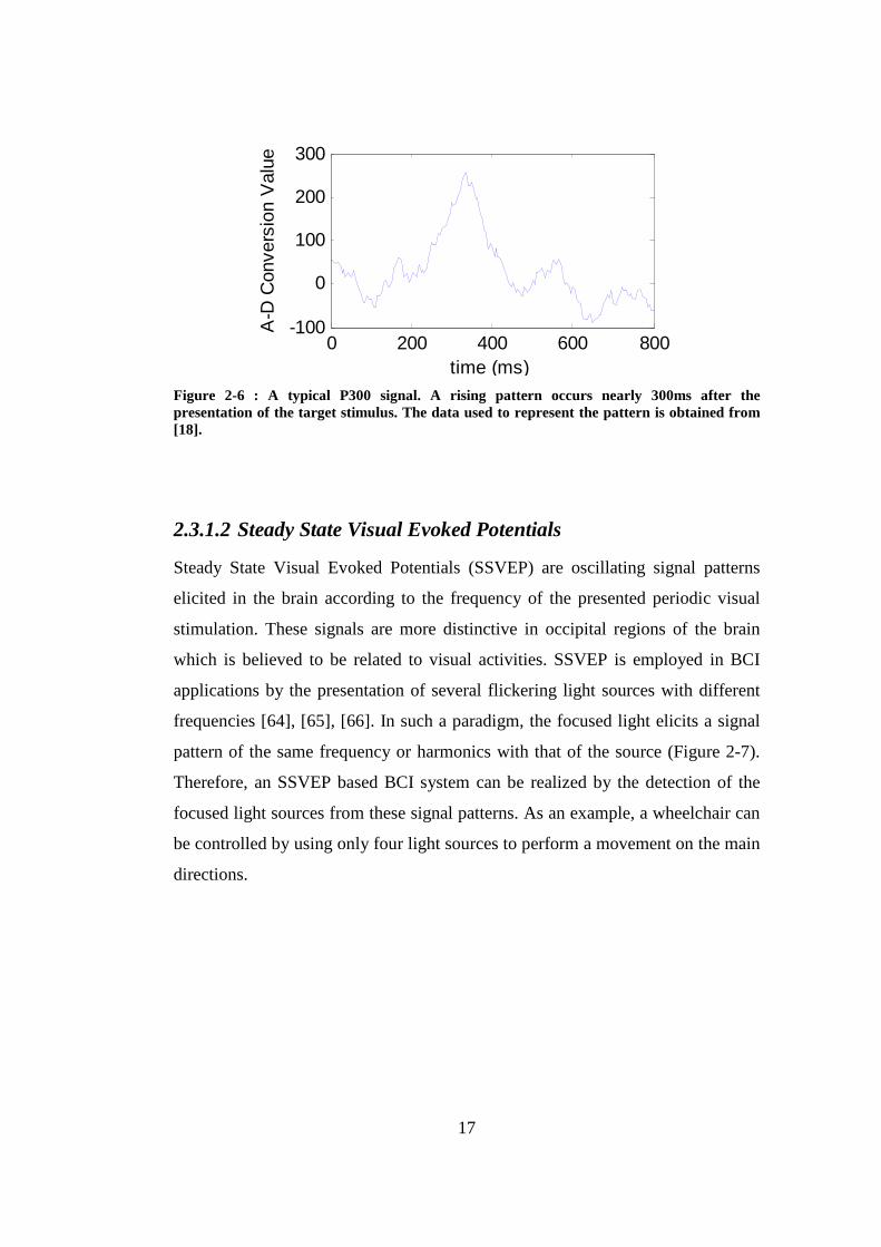
Figure 2-6 : A typical P300 signal. A rising pattern occurs nearly 300ms after the presentation of the target stimulus. The data used to represent the pattern is obtained from [18]. ....................................................................................... 17
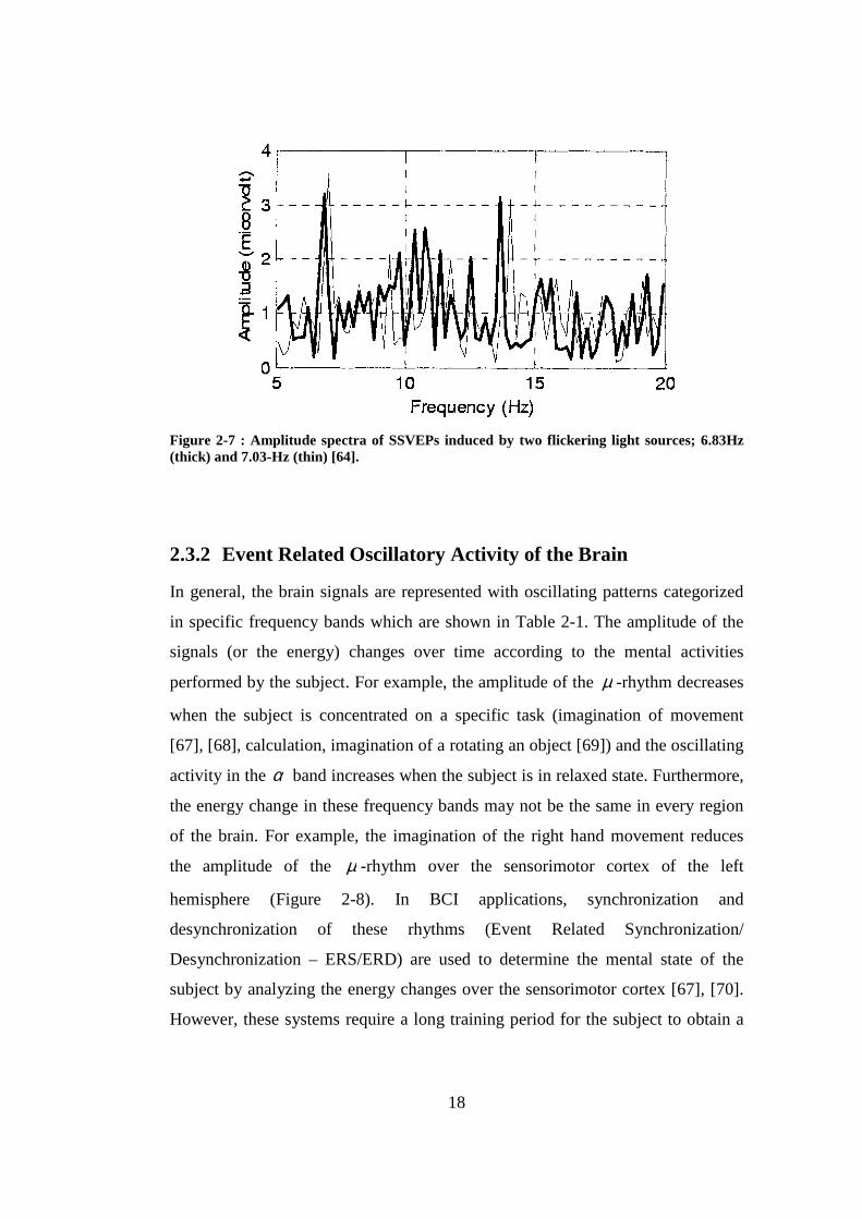
Figure 2-7 : Amplitude spectra of SSVEPs induced by two flickering light sources; 6.83Hz (thick) and 7.03-Hz (thin) [64]........................................... 18
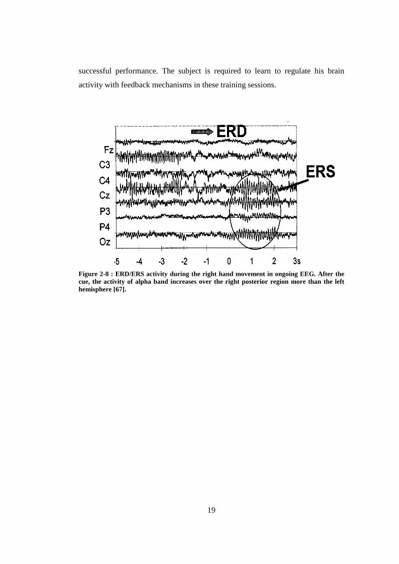
Figure 2-8 : ERD/ERS activity during the right hand movement in ongoing EEG. After the cue, the activity of alpha band increases over the right posterior region more than the left hemisphere [67].................................................... 19
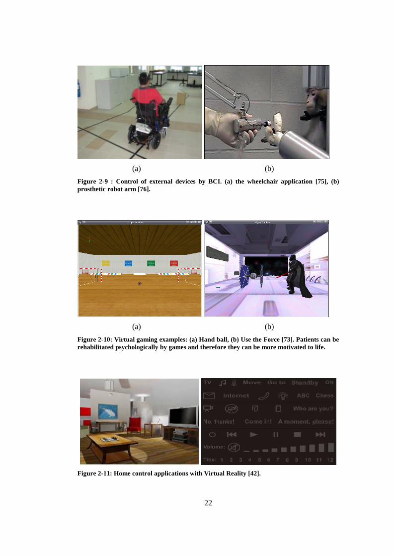
Figure 2-9 : Control of external devices by BCI. (a) the wheelchair application [75], (b) prosthetic robot arm [76]. ............................................................... 22
Figure 2-10: Virtual gaming examples: (a) Hand ball, (b) Use the Force [73]. Patients can be rehabilitated psychologically by games and therefore they can be more motivated to life........................................................................ 22
Figure 2-11: Home control applications with Virtual Reality [42]. ..................... 22 Figure 3-1: P300 Speller Matrix used in the datasets in [18] and [20]. ................ 25 Figure 4-1: The Discrete Time Model of a Practical Application. G(z): The
transfer function of the process in z-domain. d(n), x(n) and v(n) represent the desired signal, noisy observations and the additive noise respectively. ....... 32
Figure 4-2: Wiener filter model, W(z): Wiener filter to be constructed. The observations are filtered with the estimated Wiener filter which minimizes
the difference between the desired signal )(nd and the filter output )(ˆ nd .33 Figure 4-3: Averaged target responses from 10 EEG channels. The signals
averaged over parietal and central locations exhibit the presence of P300 activity. The data of [18] is used for the demonstration of the P300 signals.41

xvii
Figure 4-4: Averaged non-target responses from 10 EEG channels. The data of [18] is used to demonstrate the non-target responses. .................................. 45
Figure 4-5 : Marginal distribution of the noise signal )(nv at random time indices for the target column group. Each sample of )(nv is Gaussian like distributed with means equal to zero. ........................................................... 47
Figure 4-6 : Marginal distribution of the noise signal )(nv at random time indices for the non-target row group. Each sample of )(nv is Gaussian like distributed with means equal to zero. ........................................................... 48
Figure 4-7: The effect of Wiener filtering on a randomly selected target response. (a) Raw target signal, (b) Processed target signal with the estimated Wiener Filter.............................................................................................................. 50
Figure 4-8: The effect of Wiener filtering on a randomly selected non-target response. (a) Raw non-target signal, (b) Processed non-target signal with the estimated Wiener Filter................................................................................. 51
Figure 5-1: Visualization of a linear discriminant function for a 2-class separable problem. ........................................................................................................ 56
Figure 5-2: Relation between the function value of the sample x and its distance to the discriminating hyperplane....................................................................... 57
Figure 5-3 : Transformation between input, feature and output spaces. The feature space is constructed by performing preprocessing methods (G(X)) on the input space. Classification methods are applied on the feature space. ......... 61
Figure 5-4 : Formation of the vector for the feature space as a concatenation of time segments from 10 EEG channels .......................................................... 63
Figure 5-5 : Several solutions of the discriminating function for a linearly separable 2 category classification problem. The solution found by SVM (represented with h0) is the one that maximizes the margin between the samples (support vectors) and the hyperplane. ............................................. 64
Figure 5-6: Optimum Separating Hyperplane (OSH) of SVM for a two class case. The closest samples to OSH from each class are called the support vectors.65
Figure 6-1 : Frequency characteristics of the designed active electrodes. a) Magnitude response (in dB), b) Phase response (in degrees) ....................... 82
Figure 6-2 : Frequency characteristics of the employed active 50Hz band-stop filter. a) Magnitude response (in dB), b) Phase response (in degrees) ......... 84
Figure 6-3 : Frequency characteristics of the designed 3rd order active 40Hz low-pass filter. a) Magnitude response (in dB), b) Phase response (in degrees) . 85
Figure 6-4 : International 10 – 20 Electrode Placement System. The naming comes from the percentage ratio of the distance between two consecutive electrodes according to the distance between Inion and Nasion points of the human scalp [41]........................................................................................... 88
Figure 6-5: 19 Channel EEG cap produced by Compumedics Neuroscan [81]. .. 88 Figure 6-6 : The effect of the designed EEG cap on reducing the common mode
voltage induced on the body. The common mode voltage with respect to the amplifier ground is decreased as the distance between the amplifier ground and the electrode leads is small. Furthermore, the leakage currents are more likely to flow through the cap instead of the body with this configuration. . 89
xviii
Figure 6-7 : Pictures of the designed EEG cap. The active electrodes can easily be placed onto the scalp of the subject. ............................................................. 90
Figure 6-8: The flowchart of the controller software. MCU stands for the microcontroller unit which is the PIC18F4553 device [79].......................... 91
Figure 6-9 : Signal monitoring interface of the designed system. It is operated with the P300 Speller user interface. ............................................................ 93
Figure 6-10 : Graphical user interface prepared for the P300 Speller. ................. 94 Figure 7-1 : The EEG channels used in the measurements in P300 Speller datasets
of [18] and [20]. ............................................................................................ 97 Figure 7-2 : Epoch information in [18] and [20]. The row and column
intensifications are epoched with the ongoing EEG during the paradigm according to the demonstrated encoding scheme.......................................... 97
Figure 7-3: The electrode configurations used in existing P300 Speller Systems [42]................................................................................................................ 99
Figure 7-4 : Estimated Wiener filters for the predetermined 10 EEG channels. Wiener filter estimates are shown in red and blue for the row and column groups, respectively. In some channels the filter estimates for both groups overlap (Cz, P3 and PO8). .......................................................................... 102
Figure 7-5: Prediction accuracy of the target characters on the training set (39 characters). Solid: preprocessed with 10th order Butterworth filter. Dotted: preprocessed with 10th order FIR Wiener filter. ......................................... 104
Figure 7-6: Prediction accuracy of the target characters on the test set (31 characters). Solid: preprocessed with 10th order Butterworth filter. Dotted: preprocessed with 10th order FIR Wiener filter. ......................................... 104
Figure 7-7 : Target character prediction accuracy on the test set reported by Kaper [4]................................................................................................................ 105
Figure 7-8 : Prediction accuracy of realistic MLE of SVM outputs on the training set (39 characters). Solid: preprocessed with 10th order Butterworth filter. Dotted: preprocessed with 10th order FIR Wiener filter. ............................ 106
Figure 7-9 : Prediction accuracy of realistic MLE of SVM outputs on the test set (31 characters). Solid: preprocessed with 10th order Butterworth filter. Dotted: preprocessed with 10th order FIR Wiener filter. ............................ 107
Figure 7-10 : Pictures from the P300 Speller experiment at 9 Eylül University 108 Figure 7-11 : Estimated Wiener filters for the predetermined 10 EEG channels
(using downsampled raw EEG data). The estimates are shown in red for row, and blue for the column groups. ................................................................. 111
Figure 7-12 : Prediction accuracy of realistic MLE of SVM outputs. Preprocessed with 10th order Butterworth filter. Solid: training set (15 characters). Dotted: test set (20 characters)................................................................................. 113
Figure 7-13 : Prediction accuracy of realistic MLE of SVM outputs. Preprocessed with 8th order Butterworth filter. Solid: training set (15 characters). Dotted: test set (20 characters)................................................................................. 113
Figure 7-14 : Prediction accuracy of realistic MLE of SVM outputs. Preprocessed with 10th order Chebyshev Type I filter. Solid: training set (15 characters). Dotted: test set (20 characters).................................................................... 114
xix
Figure 7-15 : Prediction accuracy of realistic MLE of SVM outputs. Preprocessed with 8th order Chebyshev Type I filter. Solid: training set (15 characters). Dotted: test set (20 characters).................................................................... 114
Figure 7-16 : Prediction accuracy of realistic MLE of SVM outputs. Preprocessed with 10th order Wiener filter. Solid: training set (15 characters). Dotted: test set (20 characters). ...................................................................................... 115
Figure 7-17 : Prediction accuracy of realistic MLE of SVM outputs. Preprocessed with 10th order Butterworth filter, trained with optimum parameters in Table 7-7. Solid: training set (15 characters). Dotted: test set (20 characters). .... 116
Figure 7-18 : Prediction accuracy of realistic MLE of SVM outputs. Preprocessed with 8th order Butterworth filter, trained with optimum parameters in Table 7-7. Solid: training set (15 characters). Dotted: test set (20 characters). .... 116
Figure 7-19 : Prediction accuracy of realistic MLE of SVM outputs. Preprocessed with 10th order Chebychev Type I filter, trained with optimum parameters in Table 7-7. Solid: training set (15 characters). Dotted: test set (20 characters).................................................................................................................... 117
Figure 7-20 : Prediction accuracy of realistic MLE of SVM outputs. Preprocessed with 8th order Chebychev Type I filter, trained with optimum parameters in Table 7-7. Solid: training set (15 characters). Dotted: test set (20 characters).................................................................................................................... 117
Figure 7-21 : Prediction accuracy of realistic MLE of SVM outputs. Preprocessed with 10th order Wiener filter, trained with optimum parameters in Table 7-7. Solid: training set (15 characters). Dotted: test set (20 characters). ........... 118
Figure 7-22 : Estimated Wiener filters for the predetermined 10 EEG channels (estimated from the downsampled, 50Hz low-pass filtered EEG data). The estimates are shown in red for row, and blue for the column groups. ........ 119
Figure 7-23 : Prediction accuracy of realistic MLE of SVM outputs. Preprocessed with 50Hz low pass + 10th order Wiener filter, trained with the parameters of Table 7-8 (1). Solid: training set (15 characters), Dotted: test set (20 characters). .................................................................................................. 120
Figure 7-24 : Prediction accuracy of realistic MLE of SVM outputs. Preprocessed with 50Hz low pass + 10th order Wiener filter, trained with the parameters in Table 7-8 (2). Solid: training set (15 characters). Dotted: test set (20 characters). .................................................................................................. 121
Figure 7-25 : Pictures from the experiment on P300 Speller conducted in Brain Research Laboratory of Electrical and Electronics Eng. Dept., METU ..... 123
Figure 7-26 : The spelling matrix and stimulus codes used in the experimentation performed with the designed hardware....................................................... 124
Figure 7-27 : Averaged target responses measured in the P300 Speller experiment conducted with the designed hardware. ...................................................... 125
Figure 7-28 : Averaged non-target responses measured in the P300 Speller experiment conducted with the designed hardware.................................... 126
Figure 7-29 : Estimated Wiener filters for the predetermined 10 EEG channels on the experiment data performed with the designed hardware. The filters are estimated from the downsampled, 50Hz low-pass filtered EEG data and are shown in red for row, blue for the column groups...................................... 129
xx
Figure 7-30 : Prediction accuracy of realistic MLE of SVM outputs on the experiment data. Preprocessed with 50Hz low pass + 10th order Wiener filter, trained with the optimal parameters. Solid: training set (9 characters). Dotted: test set (11 characters).................................................................... 130
Figure 8-1: A compact BCI system for the disabled. In the future work, different BCI paradigms can be implemented on a single hardware system in which the basic needs of the patients are satisfied. ............................................... 137
Figure B - 1: Circuit diagram of the active electrode ......................................... 150 Figure B - 2: The pictures of the active electrodes. The electrode with the ring
shaped contact is used for reference and attached to the right ear.............. 150 Figure B - 3: The preamplifier circuitry in the EEG amplifier. .......................... 151 Figure B - 4: Active 50Hz notch filter. It is used to remove the effect of the power
line noise. .................................................................................................... 152 Figure B - 5: 3rd order Bessel low-pass filter with 40Hz cut-off frequency. ...... 152 Figure B - 6: The circuit diagram of the designed EEG amplifier. .................... 153 Figure B - 7: Pictures of the printed EEG amplifier. The system is supplied by two
batteries. These supplies are regulated with a power circuitry included in the black box..................................................................................................... 154
Figure B - 8: The circuit used in the digital hardware. The circuit is mainly composed of a compact microcontroller, PIC18F4553, which is used to perform A/D conversion and USB transfer. ............................................... 155
Figure B - 9: Pictures of the digitizing system. The analog signals are digitized by A/D conversion and sent to the computer via USB. ................................... 156
Figure B - 10: Pictures from the experiments performed with the designed EEG system. ........................................................................................................ 157
Figure B - 11 Magnitude response of the designed EEG system. The system has maximum gain between 1 and 10 Hz.......................................................... 158
Figure B - 12: Common Mode Rejection Ratio (CMRR) of the designed EEG amplifier. The system exhibits rejection of the common mode signal higher than 80dB in the frequency range of 0.1-20Hz........................................... 159
Figure B - 13: The output of the EEG system for a 100uV test signal with frequency 5Hz............................................................................................. 160
Figure B - 14: The output of the EEG system for a 100uV test signal with frequency 10Hz........................................................................................... 160
Figure B - 15: The output of the EEG system for a 100uV test signal with frequency 17Hz........................................................................................... 161
Figure B - 16: Offline visualization of the spontaneous EEG signal recorded by the system from 10 channels....................................................................... 161

1
CHAPTER 1
INTRODUCTION
Interaction with the outside world by means of communication is one of the most
indispensible gifts of the human being. We all need our hands to control or use
anything around us, legs to move and other necessary limbs that are crucial for
continuing our lives. Unfortunately, these abilities can be lost due to possible
accidents or diseases. As examples, Amyotrophic Lateral Sclerosis (ALS),
brainstem stroke and multiple sclerosis are some of the diseases in which the
motor neural pathways are damaged causing people to be locked into their bodies.
In such a case, the voluntary control is lost fully or partially over the body [1].
With full consciousness, the patients suffering from these diseases can not even
realize a physical movement or communicate with their environment. Therefore,
it is impossible for these people to live and fulfill their daily needs without
external help.
Fortunately, with the advancements in technology, researchers have developed
innovative solutions to facilitate and improve the life quality of these patients.
Among these, a well known emerging technology and research field is the Brain
Computer Interface (BCI), in which people are able to communicate with their
environment and control prosthetic or other external devices by using only their
brain activity. In a BCI system, the brain activity is translated into simple
commands using brain activity measurement systems, signal processing methods
and classification techniques with the help of neurophysiologic experimental
2
paradigms. There are also other human computer interaction systems that rely on
the movement of healthy limbs (eye-gaze etc.) as the controller of basic actions
and these systems are still more efficient than currently existing BCI systems.
However, for patients suffering from degenerative diseases like ALS, BCI is
considered as the only way of communication with the outside world.
Over the last two decades, there have been numerous studies performed on BCI.
Researchers proposed various methodologies, extended the application fields of
BCI and investigated the physiological nature of the experimental paradigms [1].
However, the main challenge in BCI is to improve the usability and practicality of
these systems. Thus, researchers put most of their effort on developing new
algorithms to improve the speed and accuracy of the prediction mechanisms in
BCI applications. Due to the nature of existing BCI’s, the applications are
considered as pattern recognition problems and variety of signal processing,
feature extraction and pattern classification techniques are being experimented in
these systems [2]. Moreover, despite the technological developments, current BCI
systems are only usable in the laboratory environment. Current studies aim to
improve these systems by building intelligent house systems in order for BCI to
be available for daily use according to the needs of the patients [11 – 15].
1.1 Scope of the Thesis
This thesis is restricted to one of the applications of BCI which is known as the
Spelling Paradigm (also known as the P300 Speller). First introduced by Farwell
and Donchin in 1988 [3], Spelling Paradigm enables paralyzed people to express
their thoughts and feelings by spelling the words on a computer screen (see
chapter 3 for a detailed description of the paradigm and previous studies). In this
application, it is aimed to predict the characters that the subject thinks of by
presenting some visual stimuli to the subject. In order to accomplish this task, the
brain activity is acquired by using biopotential measurement devices (usually via
Electroencephalography - EEG) and further analyzed with advanced signal

3
processing and classification methods. Like in all other BCI applications, the
main challenge here is to improve the accuracy and the speed of the prediction
mechanisms so that the subject can express his thoughts in a fluent manner.
In this thesis, it is intended to develop a P300 based BCI by realizing the spelling
application which can also be used in out-of-laboratory environments. The thesis
includes the design of a portable 10 channel EEG data acquisition system, the
development of signal processing methods and application of machine learning
techniques on this paradigm.
1.2 Focus and Contributions of the Thesis
The thesis focuses on some key points that are believed to be open for progress in
this application. These are stated as follows:
• Investigation of the human perception to row and column intensifications:
Existing P300 Speller systems employ row and column intensification
principle for increasing the speed of the application (see Chapter 3). In the
studies performed for this application, the responses for both row and column
stimuli are treated in the same preprocessing and classification scheme [4-10].
However, no study has been performed on the application of signal processing
and classification methods separately on these two intensification types. In
this thesis, it is aimed to investigate the difference in human perception to row
and column intensifications in P300 Speller according to the differences in
classification accuracy.
• Investigation of optimal frequency bands for the P300 Speller:
The EEG signals acquired for this application are usually filtered with a
preprocessing stage. The signal processing methods applied for this study are
mainly simple filtering techniques. In this thesis study, the optimal temporal

4
frequency bands for user specific P300 responses will be investigated by the
application of Wiener filtering in this problem.
• Estimation of probability densities in binary classification between trials:
The determination of the focused character in Spelling Paradigm is performed
by using repetitive trials and ensemble averaging in order to reduce the errors
in prediction. Unlike the common approach of assigning classification score
between trials [4], the class conditional probability density of the predicted
characters is estimated by using the Maximum Likelihood Estimation and the
target character is predicted with Bayesian decision techniques.
• Experimenting Active Electrodes in EEG measurements:
Existing BCI systems use commercial EEG devices in which the electrodes
are usually made up of ring shaped silver chloride (AgCl) leads. These
electrodes are passive conductive elements and the quality of their material
highly affects the performance of the measuring system. Moreover, employing
these in EEG measurements requires a preparation stage in which the
electrodes are covered with a conductive paste. This paste usually dries out in
a 2-3 hours of time which makes the passive electrodes unsuitable for
continuous EEG recording in BCI applications. In this thesis work, a design of
active electrodes for EEG measurements is performed to improve the quality
of the recorded EEG signals, eliminate the preparation stage required in their
passive counterparts and therefore realize a continuous EEG measurement in
BCI applications.
• EEG cap design:
Commercial EEG systems also provide electrode caps to attach the conductive
leads to the scalp of the subject. These EEG caps are usually made of elastic
silk material which can be easily stretched and fit to the subject’s head.
However, it is hard to attach the designed active electrodes on these caps. In
addition, some modifications are possible that can theoretically improve the

5
quality of the measurements in the system. Therefore, in this thesis, a shielded
EEG cap design is performed which allows easy placement of the active
electrodes on the scalp while reducing the electrical noise in the
measurements.
1.3 Outline of the Thesis
The thesis is composed of two introductory parts discussing the current BCI
systems and spelling application and three main chapters including the
methodologies performed for P300 Speller in this study.
The Brain-Computer Interface systems are introduced in chapter 2. The brain
activity measurement techniques, neurophysiologic phenomenon underlying the
principle of these systems and some BCI applications are briefly explained in this
chapter.
In chapter 3, the application of P300 Speller is presented. The experimental setup
and the review of the methodologies in the literature are provided discussing the
complexity of the approaches and success of these in literature.
The approach of Wiener filtering is discussed in chapter 4. The derivations in
Wiener filtering model and the application procedures related to P300 Speller are
explained.
In chapter 5, the classification methods used in this study are explained. The
basics of the algorithms are discussed providing correlations to the P300 Speller.
Chapter 6 is reserved for the description of the Electroencephalographic data
acquisition system designed in this study. In this chapter, the parts of the designed
system are explained briefly.

6
Chapter 7 provides the results of the proposed methodologies on one of the
Spelling Paradigm datasets in the literature and on two P300 Speller
experimentations performed in this study.
Finally in chapter 8, all of the work performed during this study is summarized.
General observations are outlined with a discussion part. The advantages of the
methods suggested in the thesis are stated and concluding remarks are given on
the experimental results. The future studies are presented by discussing the
possible modifications and improvements to implement a compact BCI system.

7
CHAPTER 2
BRAIN COMPUTER INTERFACES
In chapter 1, a brief introduction is given on Brain-Computer Interface (BCI)
technology. A formal definition of a BCI is given in [44] as a system that does not
depend on normal neural or muscular peripheral pathways of the brain. This
definition discriminates BCI from other Human-Machine Interaction (also called
Human-Machine Interface – HMI, Human-Computer Interface - HCI) systems
which rely on the movement of some healthy limbs of the body as discussed
previously. A BCI system interprets the brain activity as simple commands and
transforms these into prescribed actions within its applications (for the control of
a wheelchair as an example). Furthermore, the BCI technology is not restricted
only to the activity of the brain. The research topics also include the neural
prosthesis in which the damaged neurons can be replaced with artificial ones or
unhealthy limbs are assisted by prosthetic devices [45].
In this chapter, it is aimed to provide the necessary information related to the
underlying principles of BCI, approaches in detecting the brain activity and the
applications of BCI in real life. The chapter is concluded with a comparison of
existing BCI systems providing the efficiency and usability of these in real world
applications. The reader can find detailed information about existing BCI systems
in [1] and [46].
8
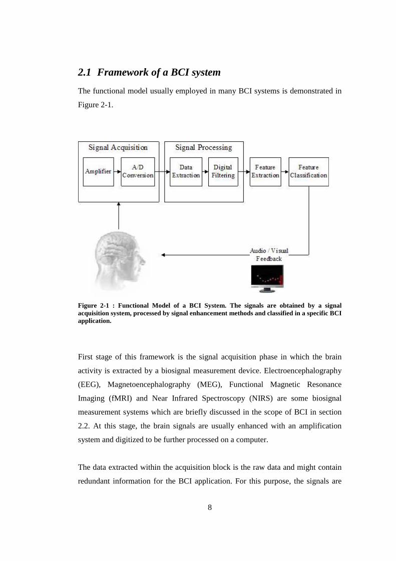
2.1 Framework of a BCI system
The functional model usually employed in many BCI systems is demonstrated in
Figure 2-1.
Figure 2-1 : Functional Model of a BCI System. The signals are obtained by a signal acquisition system, processed by signal enhancement methods and classified in a specific BCI application.
First stage of this framework is the signal acquisition phase in which the brain
activity is extracted by a biosignal measurement device. Electroencephalography
(EEG), Magnetoencephalography (MEG), Functional Magnetic Resonance
Imaging (fMRI) and Near Infrared Spectroscopy (NIRS) are some biosignal
measurement systems which are briefly discussed in the scope of BCI in section
2.2. At this stage, the brain signals are usually enhanced with an amplification
system and digitized to be further processed on a computer.
The data extracted within the acquisition block is the raw data and might contain
redundant information for the BCI application. For this purpose, the signals are

9
digitally filtered in the preprocessing stage. In this block, the unnecessary
information is eliminated by data selection (e.g. channel selection in EEG) and
several other operations (noise reduction, downsampling etc.) are performed to
improve the signal quality.
The feature extraction is the stage in which the most relevant information for
classifying the EEG patterns is investigated. Depending on the complexity of the
BCI application, the feature extraction is performed either manually or with the
application of optimization algorithms (see section 5.2.3). The aim of this stage is
to improve the classification performance of the BCI system and it is usually
performed together with the classification stage. Therefore, it can also be
considered as a preprocessing or classification method. However, it is usual to
express this stage in a separate block indicating the connection with the
preprocessing and classification phases.
The features extracted from the feature extraction block are classified in the
classification stage in order to decide which action should be taken. This block is
the main part of the system in which pattern recognition algorithms are used to
learn and model the input-output relationship of the BCI application. The
performance of a BCI system usually depends on the accuracy of the employed
classifiers.
Some BCI applications require feedback mechanisms in which some visual or
auditory signals are presented to the subject indicating the decision taken by the
classifier. The subject may need to manipulate his/her actions in performing the
mental tasks according to the given feedback in order to present accurate signals
for that application. Therefore, a feedback block may be realized with a graphical
user interface on the computer screen in a BCI application.
There are also other blocks like the external device in which the control of a
wheelchair or a prosthetic arm can be realized. These are secondary mechanisms

10
which may be integrated in the feedback stage. The presented building blocks in
Figure 2-1 are considered as the main identifiers of a BCI system and used by
many BCI researchers [14], [46], [47].
2.2 Measuring the Brain Activity
Depending on the purpose, there are several methods to measure the brain
activity. These are mainly electrical, magnetic or hemodynamic activity
measurements which are discussed briefly in the following subsections. A review
of these methods in BCI can be found in [63].
2.2.1 Electromagnetic Activity of the Brain
2.2.1.1 Electroencephalography
Electroencephalography (EEG) is one of the methods to measure the electrical
activity of the brain. The name was given after a German scientist named Hans
Berger who announced the first EEG recording in 1924 [74]. It is used widely in
clinical applications and preferred by many BCI communities as the EEG
instrumentation is relatively cheaper and portable. Furthermore, the application
procedure of EEG takes comparably less amount of time which makes it easy to
operate for BCI applications in any environment.
11
(a) (b)
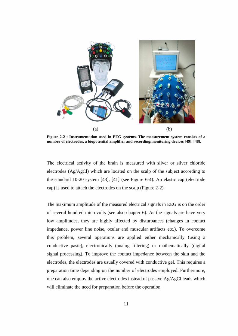
Figure 2-2 : Instrumentation used in EEG systems. The measurement system consists of a number of electrodes, a biopotential amplifier and recording/monitoring devices [49], [48].
The electrical activity of the brain is measured with silver or silver chloride
electrodes (Ag/AgCl) which are located on the scalp of the subject according to
the standard 10-20 system [43], [41] (see Figure 6-4). An elastic cap (electrode
cap) is used to attach the electrodes on the scalp (Figure 2-2).
The maximum amplitude of the measured electrical signals in EEG is on the order
of several hundred microvolts (see also chapter 6). As the signals are have very
low amplitudes, they are highly affected by disturbances (changes in contact
impedance, power line noise, ocular and muscular artifacts etc.). To overcome
this problem, several operations are applied either mechanically (using a
conductive paste), electronically (analog filtering) or mathematically (digital
signal processing). To improve the contact impedance between the skin and the
electrodes, the electrodes are usually covered with conductive gel. This requires a
preparation time depending on the number of electrodes employed. Furthermore,
one can also employ the active electrodes instead of passive Ag/AgCl leads which
will eliminate the need for preparation before the operation.
12
2.2.1.2 Electrocorticogram and Cortical Microelectrodes
Electrocorticogram (ECoG) is an invasive method in which the electrical signals
of the brain are measured under the skull, from the surface of the cortex (Figure
2-3).
(a) (b)
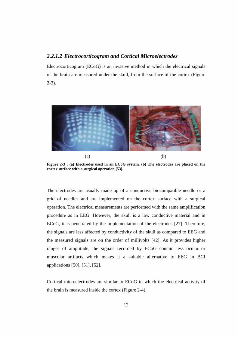
Figure 2-3 : (a) Electrodes used in an ECoG system. (b) The electrodes are placed on the cortex surface with a surgical operation [53].
The electrodes are usually made up of a conductive biocompatible needle or a
grid of needles and are implemented on the cortex surface with a surgical
operation. The electrical measurements are performed with the same amplification
procedure as in EEG. However, the skull is a low conductive material and in
ECoG, it is penetrated by the implementation of the electrodes [27]. Therefore,
the signals are less affected by conductivity of the skull as compared to EEG and
the measured signals are on the order of millivolts [42]. As it provides higher
ranges of amplitude, the signals recorded by ECoG contain less ocular or
muscular artifacts which makes it a suitable alternative to EEG in BCI
applications [50], [51], [52].
Cortical microelectrodes are similar to ECoG in which the electrical activity of
the brain is measured inside the cortex (Figure 2-4).
13
(a) (b)
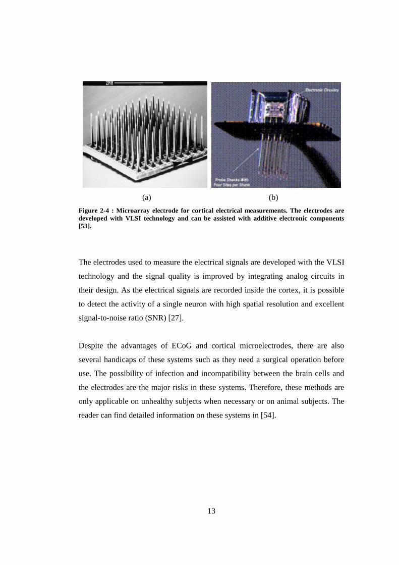
Figure 2-4 : Microarray electrode for cortical electrical measurements. The electrodes are developed with VLSI technology and can be assisted with additive electronic components [53].
The electrodes used to measure the electrical signals are developed with the VLSI
technology and the signal quality is improved by integrating analog circuits in
their design. As the electrical signals are recorded inside the cortex, it is possible
to detect the activity of a single neuron with high spatial resolution and excellent
signal-to-noise ratio (SNR) [27].
Despite the advantages of ECoG and cortical microelectrodes, there are also
several handicaps of these systems such as they need a surgical operation before
use. The possibility of infection and incompatibility between the brain cells and
the electrodes are the major risks in these systems. Therefore, these methods are
only applicable on unhealthy subjects when necessary or on animal subjects. The
reader can find detailed information on these systems in [54].
14
2.2.1.3 Magnetoencephalography
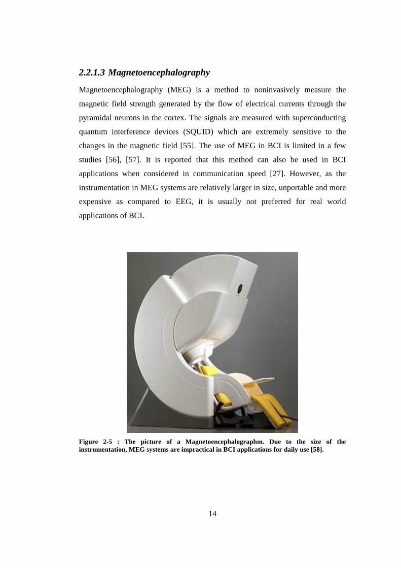
Magnetoencephalography (MEG) is a method to noninvasively measure the
magnetic field strength generated by the flow of electrical currents through the
pyramidal neurons in the cortex. The signals are measured with superconducting
quantum interference devices (SQUID) which are extremely sensitive to the
changes in the magnetic field [55]. The use of MEG in BCI is limited in a few
studies [56], [57]. It is reported that this method can also be used in BCI
applications when considered in communication speed [27]. However, as the
instrumentation in MEG systems are relatively larger in size, unportable and more
expensive as compared to EEG, it is usually not preferred for real world
applications of BCI.
Figure 2-5 : The picture of a Magnetoencephalographm. Due to the size of the instrumentation, MEG systems are impractical in BCI applications for daily use [58].

15
2.2.2 Hemodynamic Activity of the Brain
2.2.2.1 Functional Magnetic Resonance Imaging
Functional Magnetic Resonance Imaging (fMRI) is a method used to measure the
amount of oxygen in the blood flowing through the brain. When the neurons are
active, the consumption of oxygen increases in these cells. Therefore, this gives
an idea about the neural activity in different regions of the brain. The spatial
resolution in this technique is comparably higher than that of others. In fact, the
neural activity can be detected not only from the cortex but also any other regions
of the brain. On the other hand, the fMRI systems have a poor temporal
resolution; the response of hemodynamic activity is extracted within a few
seconds [27]. In addition, the equipments in these systems are larger in size and
much more expensive. Therefore, it is nearly impossible to employ fMRI in BCI
applications for daily use. Nevertheless, researchers investigated fMRI to observe
the hemodynamic activity in BCI applications [59], [60], [61].
2.2.2.2 Near Infrared Spectroscopy
Similar to fMRI, Near Infrared Spectroscopy (NIRS) is used to measure the
hemodynamic activity of the brain. The principle of this technique is to detect the
amount of blood oxygen in the brain from the reflection of the emitted infrared
light. As the hemodynamic activity is measured, the temporal resolution is poor in
NIRS systems, which makes the method impractical for BCI applications.
However, few BCI studies were performed with NIRS which basically investigate
the suitability of this brain activity measuring method in BCI applications [27],
[62].

16
2.3 Neurophysiologic Background of BCI
There are various implementations of BCI, relying on different physiological
activities related to human brain. Basically, there are three main approaches
employed in existing BCI systems. The first approach is based on the responses of
the subject to some external stimuli which are known as Event Related Potentials.
In the second approach, the subject regulates the brain activity by concentrating
on specific mental tasks. Slow Cortical Potentials (SCP) is the final method which
is based on the slow potential shifts in the brain observed according to the mental
state of the subject. Here, only the first two approaches will be briefly described
as the method of SCP is not of interest in current BCI studies.
2.3.1 Event Related Potentials
Event Related Potentials are specific patterns occurring after or during the
presentation of an auditory or visual stimulus. These include the P300 patterns
and Steady State Visual Evoked Potentials (SSVEP).
2.3.1.1 P300 Signals
P300 is a peaking signal pattern which occurs after the presentation of a rare
audio/visual event [3], [16] (Figure 2-6). It is observed nearly 300ms after the
stimulus onset which gives the name to the signal pattern. Such a phenomenon
occurs when the subject is asked to focus attention on a specific stimulus (also
named as the target or odd-ball) which is rarely encountered among a large
number of other irrelevant stimuli (non-target). Furthermore, the evoked P300
response is more distinctive when the occurrence of the event is random. The idea
is first investigated in BCI in [3] with a spelling application which is explained in
chapter 3 in detail.
17
0 200 400 600 800-100
0
100
200
300
time (ms)
A-D
Con
vers
ion
Val
ue
Figure 2-6 : A typical P300 signal. A rising pattern occurs nearly 300ms after the presentation of the target stimulus. The data used to represent the pattern is obtained from [18].
2.3.1.2 Steady State Visual Evoked Potentials
Steady State Visual Evoked Potentials (SSVEP) are oscillating signal patterns
elicited in the brain according to the frequency of the presented periodic visual
stimulation. These signals are more distinctive in occipital regions of the brain
which is believed to be related to visual activities. SSVEP is employed in BCI
applications by the presentation of several flickering light sources with different
frequencies [64], [65], [66]. In such a paradigm, the focused light elicits a signal
pattern of the same frequency or harmonics with that of the source (Figure 2-7).
Therefore, an SSVEP based BCI system can be realized by the detection of the
focused light sources from these signal patterns. As an example, a wheelchair can
be controlled by using only four light sources to perform a movement on the main
directions.
18
Figure 2-7 : Amplitude spectra of SSVEPs induced by two flickering light sources; 6.83Hz (thick) and 7.03-Hz (thin) [64].
2.3.2 Event Related Oscillatory Activity of the Brain
In general, the brain signals are represented with oscillating patterns categorized
in specific frequency bands which are shown in Table 2-1. The amplitude of the
signals (or the energy) changes over time according to the mental activities
performed by the subject. For example, the amplitude of the µ -rhythm decreases
when the subject is concentrated on a specific task (imagination of movement
[67], [68], calculation, imagination of a rotating an object [69]) and the oscillating
activity in the α band increases when the subject is in relaxed state. Furthermore,
the energy change in these frequency bands may not be the same in every region
of the brain. For example, the imagination of the right hand movement reduces
the amplitude of the µ -rhythm over the sensorimotor cortex of the left
hemisphere (Figure 2-8). In BCI applications, synchronization and
desynchronization of these rhythms (Event Related Synchronization/
Desynchronization – ERS/ERD) are used to determine the mental state of the
subject by analyzing the energy changes over the sensorimotor cortex [67], [70].
However, these systems require a long training period for the subject to obtain a
19
successful performance. The subject is required to learn to regulate his brain
activity with feedback mechanisms in these training sessions.
Figure 2-8 : ERD/ERS activity during the right hand movement in ongoing EEG. After the cue, the activity of alpha band increases over the right posterior region more than the left hemisphere [67].

20
Table 2-1: Oscillatory EEG wave patterns and their frequency ranges [74].
Wave Frequency
Range
Characteristics
delta - δ 0 – 4 Hz • slow wave sleep for adults
• seen in babies
theta - θ 4 – 7 Hz • seen in young children
• drowsiness or arousal in older children and adults
• idling, meditation
alpha -α 8 – 12 Hz • relaxed/reflecting
• occurs usually when closing the eyes
beta - β 12 – 30 Hz • alert state, working
• active, busy or anxious thinking, active
concentration
gamma - γ 30 – 100 Hz • alert state, working
• seen when a certain cognitive or motor functions is
employed
mu - µ ~10Hz • alpha range activity indicating the imagination of
movement when it is attenuated.

21
2.4 Applications and Potential Users of BCI
Depending on the purpose, a BCI system can find many different application
fields (bioengineering, military, gaming industry etc.). As its primary objective, a
BCI can be used to assist a disabled person by providing a control on an external
device so that he/she can realize specific actions like movement via wheelchair,
control of a prosthetic arm and house control systems or communication with
other people. Potential users of BCI can vary from healthy subjects to severely
disabled ones like ALS patients.
Table 2-2: Potential Users of BCI in the world [42].
Type of the Disease Number of Patients
Amyotrophic Lateral Sclerosis (ALS) 400,000/3,000,000
Multiple Sclerosis 2,000,000
Muscular Dystrophy 1,000,000
Brainstem Stroke 10,000,000
Cerebral Palsy 16,000,000
Spinal Cord Injury 5,000,000
Postpolio Syndrome 7,000,000
Guillain-Barre Syndrome 70,000
Other types of Stroke 60,000,000
A BCI system can also be used in rehabilitation of these patients by encouraging
and motivating them to life with virtual reality and gaming applications [72], [73].
Although these applications do not provide primary needs of the subjects, they
improve the life quality of these patients in psychological point of view.
22
(a) (b)
Figure 2-9 : Control of external devices by BCI. (a) the wheelchair application [75], (b) prosthetic robot arm [76].
(a) (b)
Figure 2-10: Virtual gaming examples: (a) Hand ball, (b) Use the Force [73]. Patients can be rehabilitated psychologically by games and therefore they can be more motivated to life.
Figure 2-11: Home control applications with Virtual Reality [42].
23
2.5 Conclusion
As existing BCI systems are compared to each other, all approaches explained in
section 2.3 have similar performances in prediction accuracy and speed in most of
the subjects. Each approach has a different advantage regarding the
implementation of the applications or time required to operate the BCI. For
example, it is difficult and impractical to control a wheelchair with a P300 based
BCI; an ERD/ERS or SSVEP based BCI can provide a faster control on a
wheelchair or prosthetic hand application. However, P300 based BCI’s do not
require subject training as in the case of motor imagery BCI systems. The training
time required in motor imagery BCI’s can be as long as 6 months to successfully
operate the system [42].
The major drawback of P300 and SSVEP based BCI’s is that a visual stimulation
is needed to operate these systems. When considered in that point of view,
ERD/ERS based BCI systems have the advantage of operation without external
stimulation. On the other hand, it is usually harder to detect the ERD/ERS activity
than P300 responses. Furthermore, P300 based systems provide higher degrees of
freedom in the applications. That is, with SSVEP or motor imagery BCI, it is
impractical to implement an application that includes 36 or more different
possibilities (the spelling application or smart home control). Regarding all these
points, one can decide on the type of the BCI in order to implement a specific
paradigm. Therefore, the main consideration here is to determine the feasibility of
the approaches on the BCI application that is to be implemented.
24
CHAPTER 3
SPELLING PARADIGM
Although chapter 1 provided an introductory description of the P300 Speller,
here, it is aimed to explain this BCI application within a separate chapter. The
chapter starts with a detailed explanation of the experimental setup and then
continues with a brief review of the previous studies performed on this title.
Finally, a concluding section is provided at the end of the chapter discussing the
accuracy and complexity of reviewed methodologies.
3.1 Experimental Setup
In the experimental paradigm proposed by Farwell and Donchin [3], a 6 by 6
matrix of alphanumeric characters is presented to the subject on a computer
screen (see Figure 3-1 for a spelling matrix example). The rows and columns of
this matrix are sequentially intensified in a random order with a predefined
duration and interstimulus interval (the duration between two consecutive
intensifications). The subject is asked to focus attention on a specific character
and is assumed to count the number of intensifications whenever the row or
column containing the focused character is flashed. The focused characters here
will be named as the target characters and consequently, the row and column
intensifications containing the target character will be referred as the target
intensifications throughout the thesis.

25
Figure 3-1: P300 Speller Matrix used in the datasets in [18] and [20].
The row and column intensifications in fact constitute the visual stimulations in
this paradigm. Moreover, there are few target stimulations as compared to the
non-target ones. For example, for a 6 by 6 matrix of characters, there is only one
target row intensification and one column intensification since the target character
is in the intersection of these two stimuli. The other five rows and five columns
constitute the non-target intensifications and the responses of the subject to these
stimulations are supposed to be different than that of the target ones. The
underlying principle of the spelling application is that the subject produces
specific responses to the target intensifications as they occur less than the non-
target ones. The target stimulations are expected to evoke the so called P300
potential which is described in section 2.3.1.1.

26
The very aim of this application is to predict the target character such that the
subject expresses his/her thoughts fluently by spelling the words on the screen. In
order to accomplish this task, the algorithms try to determine the stimulations that
evoked the P300 responses (i.e. the target responses) and therefore predict the
character that the subject focused. However, usually it is difficult to make this
prediction in one trial which corresponds to the duration that all the rows and
columns of the matrix are intensified only once. The reason is that the measured
EEG signals are highly affected by noise and this makes it impossible to
distinguish the target responses from the non-target ones within a single trial.
Therefore, several trials are performed for the same target character in order to
decrease the error in prediction.
Employment of trial repetition comes with the main disadvantage of duration of
prediction. That is, the more trial repetition, the longer it takes to predict the target
character which makes it unsuitable for the subject to fluently express his or her
thoughts. As an example, for the dataset of [18] experimented in this study, the
trial duration corresponds to 4.5 seconds. Using at least 5 trial repetitions for
guessing the character takes 22.5 seconds which takes a few minutes to complete
a 5-10 letter word1. Therefore, the challenge in this application is also to decrease
the time for prediction of the target characters (use less number of trial repetitions
to predict) and thus improve the usability of the system.
1 The spelling of a character in the paradigm actually depends on many factors which are explained in the results chapter. One can decrease the timing parameters which can affect the speed of the prediction mechanism. However, the consideration stated here is to minimize the number of trial repetitions which is the main factor assessing the speed of the system.
27
3.2 Preceding the Analysis
The common procedure before designing a classification model for the P300
Speller is to follow a few steps to extract the relevant information from the
provided training dataset. This involves the selection of a set of EEG channels
that are likely to exhibit the presence of a P300 response, extraction of EEG time
segments of predefined length after the stimulus onset from these channels and
the combination of stimulus code and the class label information with the
extracted EEG segments. After that, one usually applies low-pass or band-pass
filtering for better signal to noise ratio (SNR) and may employ downsampling
operation to reduce the dimensionalty of the signal.
3.3 Review of the Methodologies
As mentioned before, in BCI studies, the researchers focused mainly on the
application of different classification and signal enhancement methods in existing
BCI problems. Here, the methodologies will be briefly reviewed for P300 Speller
in terms of classification and signal processing aspects. Detailed review for the
classification problem in BCI applications can be found in [9] and [2].
3.3.1 Review of Studies in Machine Learning
Earlier studies in P300 Speller approached the pattern classification problem in
unsupervised aspects like the application of peak picking algorithms and decision
principle according to area of the EEG segment in the time domain [3], [8]. In
their pioneering work, Farwell and Donchin investigated four different
classification methodologies for categorizing the target and non-target responses
[3]. They have compared Stepwise Discriminant Analysis (SWDA), peak
detection, classification according to the area of the responses and covariance
methods for the P300 Speller. However, with the advances in technology and
increase in computation power, the application of supervised classification
28
techniques became more popular in which the algorithms are developed on a
training dataset.
Kaper et al. investigated the application of Support Vector Machines (SVM’s)
with Gaussian kernel transformation on the paradigm and obtained successful
results while using only a few number of EEG channels [4]. They have been
elected as one of the winners in BCI Competition II [17], [18] due to the success
and the simplicity of the method they have proposed. SVM has also been applied
in numerous studies for the classification of P300 responses [6], [21], [22] and in
other BCI applications [23], [24], [25]. In their work, Rakotomamonjy et al.
trained several SVM’s on different partitions of the training dataset while
recursively selecting the optimal subset of EEG channels as features [6]. They
won the BCI Competition III [19], [20] with the highest prediction accuracy on
the test set in P300 Speller.
Linear Discriminant Analysis (LDA) or more specifically Fisher’s LDA has been
investigated for P300 speller by Bostanov [7] in which the aim is to separate the
data by constructing a hyperplane between the classes. The classification method
has shown a relatively well performance for the P300 speller dataset in BCI
Competition II and elected as one of the winning methods in this contest.
In order to predict the target character in Spelling Paradigm, additional decision
methodology is needed after the application of the discriminative classifiers. This
procedure can be simply the scoring of the classifier output [4] or a more
probabilistic approach in which the classification is performed regarding the
distribution of the discriminative classifier outcome. Guan et al. conducted
research on the statistical modeling of P300 responses by analyzing the stimulus
output distribution of the main classifier [26]. They proposed probabilistic
methods for the multi-trial EEG signals and employed assumed distributions for
the discriminative classifier output (mainly Gaussian) in prediction of the target
character. Hoffman [27] studied the Bayesian algorithms in his doctoral thesis
29
work providing a well understanding of the applied procedure. He applied the
evidence framework for Bayesian regression in P300 speller [29] and proposed a
combined discriminative method named as Bayesian Discriminant Analysis
(BDA) for this problem [28]. Moreover, Lin and Zhang investigated the
classification problem in P300 Speller regarding the perceptual characteristics of
the paradigm [21]. They approached the problem in three category classification
task considering also the intensifications adjacent to target stimuli. In their study,
the accuracy of the prediction was reported to be improved when the probabilistic
model included the confusion of the subject due to these nearby target
intensifications.
3.3.2 Studies on Signal Enhancement and Feature Extraction
The preprocessing algorithms for improving the EEG signal quality play an
important role in accurate prediction of the target character in Spelling Paradigm
as well as the classification methods applied this context. Especially, the feature
extraction methods reduce the complexity of the problem by optimizing the
computational effort needed for the classifiers. These methods can be as simple as
usual low-pass or band-pass filtering or more complicated procedures which
require a solution of an optimization problem.
The method of Principle Component Analysis (PCA) has been applied in [5], [30]
to reduce the dimensionality of the data extracted from the selected EEG
channels. The idea in PCA is to determine the maximum eigenvalues which elicit
the principle components of the signal. In other words, PCA removes the
relatively irrelevant parts of the data while retaining the most powerful
components of the signal. This provides the dimensionality reduction of the
feature vector which usually improves the performance of the employed classifier.
Another signal processing technique called the Independent Component Analysis
(ICA) has been investigated in numerous studies in BCI [8], [9], [31]. Being one
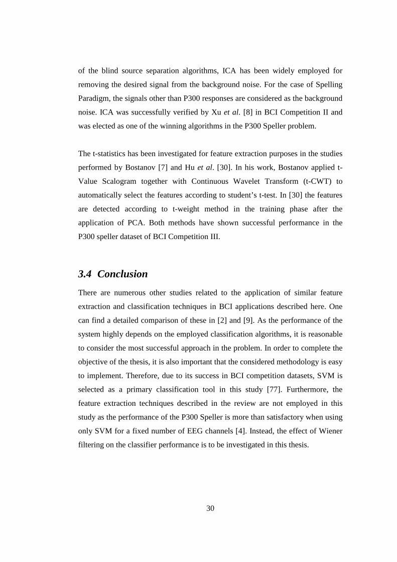
30
of the blind source separation algorithms, ICA has been widely employed for
removing the desired signal from the background noise. For the case of Spelling
Paradigm, the signals other than P300 responses are considered as the background
noise. ICA was successfully verified by Xu et al. [8] in BCI Competition II and
was elected as one of the winning algorithms in the P300 Speller problem.
The t-statistics has been investigated for feature extraction purposes in the studies
performed by Bostanov [7] and Hu et al. [30]. In his work, Bostanov applied t-
Value Scalogram together with Continuous Wavelet Transform (t-CWT) to
automatically select the features according to student’s t-test. In [30] the features
are detected according to t-weight method in the training phase after the
application of PCA. Both methods have shown successful performance in the
P300 speller dataset of BCI Competition III.
3.4 Conclusion
There are numerous other studies related to the application of similar feature
extraction and classification techniques in BCI applications described here. One
can find a detailed comparison of these in [2] and [9]. As the performance of the
system highly depends on the employed classification algorithms, it is reasonable
to consider the most successful approach in the problem. In order to complete the
objective of the thesis, it is also important that the considered methodology is easy
to implement. Therefore, due to its success in BCI competition datasets, SVM is
selected as a primary classification tool in this study [77]. Furthermore, the
feature extraction techniques described in the review are not employed in this
study as the performance of the P300 Speller is more than satisfactory when using
only SVM for a fixed number of EEG channels [4]. Instead, the effect of Wiener
filtering on the classifier performance is to be investigated in this thesis.

31
CHAPTER 4
WIENER FILTERING
As it constitutes the major subject in this thesis in terms of signal enhancement,
the method of Wiener filtering and its application to the P300 Speller are
explained in this chapter. The chapter begins with a description of the Wiener
model, and continues with the derivations required to design the optimal Wiener
filter. Finally, the Wiener approach on the spelling application is given at the end
of the chapter, explaining the application procedure for this problem.
4.1 Introduction
In many practical applications, it is of interest to reconstruct a signal from noisy
observations. However, it may be impossible to achieve this task with simple,
classical filtering techniques. In such cases, it is necessary to take the statistics
into account and apply more complex signal processing methods. Wiener filtering
is a statistical signal processing technique, in which, it is aimed to construct a
filter to estimate the desired signal from noisy observations [32]. It is a kind of
optimal filtering in the sense that it minimizes the error in the estimation of the
desired signal [33].
Depending on purpose, Wiener filter can be applied to numerous signal
processing problems. For example, in the simple filtering case, the aim is to
estimate the desired signal by designing a causal filter. There is also a noncausal
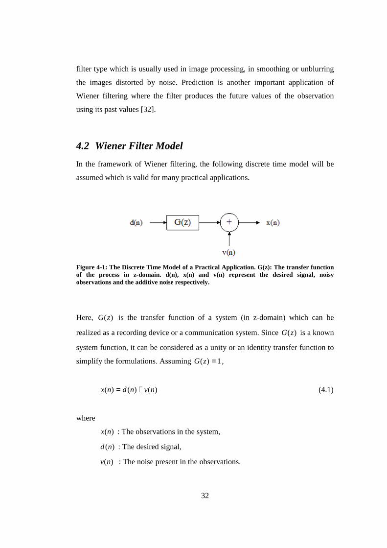
32
filter type which is usually used in image processing, in smoothing or unblurring
the images distorted by noise. Prediction is another important application of
Wiener filtering where the filter produces the future values of the observation
using its past values [32].
4.2 Wiener Filter Model
In the framework of Wiener filtering, the following discrete time model will be
assumed which is valid for many practical applications.
Figure 4-1: The Discrete Time Model of a Practical Application. G(z): The transfer function of the process in z-domain. d(n), x(n) and v(n) represent the desired signal, noisy observations and the additive noise respectively.
Here, )(zG is the transfer function of a system (in z-domain) which can be
realized as a recording device or a communication system. Since )(zG is a known
system function, it can be considered as a unity or an identity transfer function to
simplify the formulations. Assuming 1)( =zG ,
)()()( nvndnx += (4.1)
where
)(nx : The observations in the system,
)(nd : The desired signal,
)(nv : The noise present in the observations.

33
The starting assumption is that the desired signal )(nd and the observations )(nx
are jointly wide sense stationary processes (WSS) with known
autocorrelations, )(krx , )(krd and crosscorrelation )(krdx . The goal is to design a
linear, shift-invariant filter )(nw that would produce the minimum square error
(mse) estimate of the desired signal from the observations, considering the
statistics of each signal [32].
The squared error to be minimized is defined as:
})({2
neE=ξ (4.2)
where
)(ˆ)()( ndndne −= . (4.3)
Here, )(ˆ nd represents the estimated signal and )(ne is the difference between the
desired signal and the estimated signal, i.e. the error. The model is illustrated in
Figure 4-2.
Figure 4-2: Wiener filter model, W(z): Wiener filter to be constructed. The observations are filtered with the estimated Wiener filter which minimizes the difference between the desired
signal )(nd and the filter output )(ˆ nd .

34
Depending on the requirements in the filter design, Wiener filter takes different
forms considering the finite-infinite impulse response (FIR or IIR) and causality
in the filter: causal-FIR, noncausal-FIR, causal-IIR and noncausal-IIR Wiener
filter. Here, the noncausal and IIR form of the Wiener filter will be investigated in
the explanation framework of [32]. The formulations derived for the noncausal
IIR Wiener filter are also valid for other types. Detailed explanation and
derivations can be found in [32] and [33] for each type of design.
4.3 Noncausal IIR Wiener Filter Design
The noncausal IIR form of the Wiener filter can be represented in the z-domain
as:
∑∞=
−∞=
−=n
n
nznwzW )()( (4.4)
The estimate of the desired signal in Figure 4-2 is the convolution of )(nx and
)(nw ,
∑∞
−∞=
−=∗=l
lnxlwnxnwnd )()()()()(ˆ (4.5)
In order to find the filter coefficients optimally in the mean square sense (mse),
the derivative of the squared error defined in (4.2) with respect to )(* nw or )(nw
should be equal to zero for all samples of the filter [32]. Thus,
{ }
∞<<∞−=
∂∂=
∂∂=
∂∂
∗
∗
∗∗∗
kkw
neneE
neneEkwkw
0)(
)()(
)()()()(
ξ
(4.6)

35
Combining (4.3) with (4.5), )(ne can be rewritten as
∑∞
−∞=
−−=l
lnxlwndne )()()()( (4.7)
Then the partial derivative expression in (4.6) reduces to
)()(
)(knx
kw
ne −−=∂∂ ∗
∗
∗
(4.8)
Substituting the derivative expression in (4.6) with the result found in (4.8),
{ } 0)()( =−∗ knxneE ∞<<∞− k (4.9)
Equation (4.9) is referred as the orthogonality principle or the projection theorem
[32] which implies that all of the samples of the observation are orthogonal to the
error in estimation of the desired signal. Thus, if )(ne in (4.7) is substituted in
(4.9), we obtain
{ } { } 0)()()()()( =−−−− ∑∞
−∞=
∗∗
l
knxlnxElwknxndE (4.10)
Since it is assumed that )(nx and )(nd are jointly WSS processes, the
expectation expressions in (4.10) are equal to the cross-correlation of )(nx with
)(nd and autocorrelation of )(nx respectively. Therefore, equation (4.10) can be
rewritten as
∑∞
−∞=−=
lxdx lkrlwkr )()()( ∞<<∞− k (4.11)

36
Equation (4.11) is known as the Wiener-Hopf equation for the noncausal IIR
Wiener filter. It differs from the FIR case by the limits of the summation and the
range for k for which the equation should hold [32]. Unlike the FIR Wiener filter,
the solution for )(kw can not be found directly from (4.11), since there are
infinite number of equations with infinite number of unknowns in the IIR case.
However, if the equation is turned into a convolution expression between )(kw
and )(krx , finding a solution for )(kw will be much easier:
)()()( krkwkr xdx ∗= (4.12)
If the Fourier transform is applied to (4.12), the variables can be expressed in the
frequency domain as
)()()( jwWjwPjwP xdx = (4.13)
Thus, the frequency response of the noncausal IIR Wiener filter is
)(
)()(
jwP
jwPjwW
x
dx= (4.14)
where )( jwPdx is the cross-power spectral density of the desired and observation
signals and )( jwPx is the power spectral density (psd) of the observation signal.
According to equation (4.14), the optimum Wiener filter depends only on )( jwPx
and )( jwPdx . Thus, when these are calculated, the design of the Wiener filter will
be complete.
Here, it can be assumed that )(nd and )(nv are statistically independent
processes and also )(nv is a zero mean random process. Usually, independence is
a reasonable assumption in practical applications since the desired signal may not

37
necessarily be related to the noise. Therefore, from the independence assumption
it can be inferred that they are also uncorrelated. Then, if we would like to express
the autocorrelation of )(nx ,
{ }( ) ( )( ) ( ) ( )( ){ }
{ } { } { }{ }
)()()()(
)()(
)()()()()()(
)()()(
krkrkrkr
kndnvE
knvndEknvnvEkndndE
knvkndnvndE
knxnxEkr
vddvvd
x
+++=−+
−+−+−=
−+−+=
−=
∗
∗∗∗
∗∗
∗
(4.15)
Since )(nd and )(nv are uncorrelated, their cross-correlation )(krdv or )(krvd
reduces to zero. Therefore,
)()()( krkrkr vdx += (4.16)
and the power spectral density of )(nx becomes
)()()( jwPjwPjwP vdx += (4.17)
When we consider the cross-correlation between )(nx and )(nd , it can be found
that
{ }{ } { }
)(0
)()()()(
)()()(
kr
knvndEkndndE
knxndEkr
d
dx
==
−+−=
−=∗∗
∗
44 344 21 (4.18)
Thus,
)()( jwPjwP ddx = (4.19)

38
which is valid under the assumption that )(nv is zero mean and )(nd and )(nv
are uncorrelated WSS random processes. This assumption is important especially
for the optimality of the Wiener filter. When one of the signals is found to be non-
stationary, the use of linear, shift invariant Wiener filter will not be optimum [32].
Moreover, if the noise signal has non-zero mean, then a few more terms will be
added to the cross-power spectral density, which will certainly affect the
frequency characteristics of the Wiener filter when ignored. Then, the IIR Wiener
filter takes the final form:
)()(
)(
)(
)(
)(
)()(
jwPjwP
jwP
jwP
jwP
jwP
jwPjwW
vd
d
x
d
x
dx
+=== (4.20)
To construct the Wiener filter in a specific application, one can choose any
equality expression in (4.20), considering to the computational difficulty in
evaluation of these parameters.
After finding the optimum Wiener filter, we can now evaluate the mean square
error in the estimation of the desired signal.
{ }
{ } { }44 344 21
0
)()()()()(
)()()()()(2
=−−=
−−==
∗∞
−∞=
∗∗
∗∞
−∞=
∑
∑
lnxneElwndneE
lnxlwndneEneE
l
l
ξ
(4.21)
If )(nw is the solution of Wiener-Hopf equations in (4.11) satisfying the
minimum mean squared error, then due to the orthogonality principle defined in
(4.9), the last expectation term in the summation drops to zero. Therefore,

39
{ } ( ){ }
{ } { }
)()()0(
)()()()()(
)()()()(
)()(ˆ)()()(
)()0(
min
lrlwr
ndlnxElwndndE
ndlnxlwndE
ndndndEndneE
dxl
d
lldxrdr
l
∗∞
−∞=
∞
−∞= ∗=
∗
=
∗
∗∞
−∞=
∗∗
∑
∑
∑
−=
−−=
−−=
−==
44 344 2144 344 21
ξ
(4.22)
Evaluation of the minimum mean squared error in (4.22) requires a lot of
computation due to infinite samples in the summation. However, if Parseval’s
theorem is applied to the summation in (4.22) calculations will become much
easier in the frequency domain.
∫−
∗−=π
ππξ dwjwPjwWr
dxd )()(2
1)0(min (4.23)
From the same reasoning, we can also express )0(dr as,
∫−
=π
ππdwjwPr dd )(
2
1)0( (4.24)
Therefore, the minimized mean square error becomes,
( )∫−
∗−=π
ππξ dwjwPjwWjwP
dxd )()()(2
1min (4.25)

40
4.4 Application of Wiener Filtering in P300 Speller
As discussed in chapter 3, the identification of P300 patterns from EEG is the
main goal in Spelling Paradigm. In this subchapter, the Wiener filtering approach
for the signal enhancement problem will be investigated in this context. Here, we
will treat the problem as in the following: we will construct a Wiener model for
target signals, i.e. the class of P300 patterns, and another one for non-target
signals. Then, we will combine these two systems and construct a single model
that will enhance the target signals while suppressing the non-target ones.
To begin with, the model in Figure 4-1 is assumed for the signal acquisition phase
of the P300 speller, where )(nx represents the recorded EEG data. As defined
before, )(nd and )(nv are the desired and the noise signals, respectively.
However, the desired signal here will be either the target signal, or the non-target
signal waveform depending on the system of concern. For the sake of simplicity
and clarity, we will consider the target signal system first and then continue with
the non-target one. The EEG data used for demonstrating the target and non-target
signals is from the dataset IIb of BCI Competition 2003 [18].
As averaging-between-trials is a common approach in classification in this
problem, it is natural to obtain the main target response or P300 response by
averaging all signals belonging to the target class. By averaging all target signals
in the dataset, we in fact, obtain the least square solution for P300 pattern
measured from related EEG channels. This is a well known technique for
reducing the noise present in the measurements.
Therefore, when the ensemble averaging is performed between the observations,
we obtain the target responses as given in Figure 4-3.
41
0 200 400 600 800-100
0
100
200
300Averaged P300 response, Channel C3
time (ms)
A-D
Con
vers
ion
Val
ue
0 200 400 600 800-100
0
100
200
300Averaged P300 response, Channel Cz
time (ms)
A-D
Con
vers
ion
Val
ue0 200 400 600 800
-100
0
100
200Averaged P300 response, Channel C4
time (ms)
A-D
Con
vers
ion
Val
ue
0 200 400 600 800-300
-200
-100
0
100Averaged P300 response, Channel Fz
time (ms)A
-D C
onve
rsio
n V
alue
0 200 400 600 800-200
-100
0
100
200Averaged P300 response, Channel P3
time (ms)
A-D
Con
vers
ion
Val
ue
0 200 400 600 800-200
-100
0
100Averaged P300 response, Channel Pz
time (ms)
A-D
Con
vers
ion
Val
ue
0 200 400 600 800-150
-100
-50
0
50Averaged P300 response, Channel P4
time (ms)
A-D
Con
vers
ion
Val
ue
0 200 400 600 800-200
-100
0
100Averaged P300 response, Channel PO7
time (ms)
A-D
Con
vers
ion
Val
ue
0 200 400 600 800-900
-800
-700
-600
-500Averaged P300 response, Channel PO8
time (ms)
A-D
Con
vers
ion
Val
ue
0 200 400 600 800-200
-100
0
100Averaged P300 response, Channel Oz
time (ms)
A-D
Con
vers
ion
Val
ue
Figure 4-3: Averaged target responses from 10 EEG channels. The signals averaged over parietal and central locations exhibit the presence of P300 activity. The data of [18] is used for the demonstration of the P300 signals.
42
To construct the Wiener model, we will consider the P300 response as the desired
signal )(nd . Despite the fact that )(nd has a stochastic behavior in Wiener
model, the P300 signal discussed here is somewhat a deterministic signal. In order
to take the P300 response as the desired signal, a more statistical model should be
included in the P300 response.
Therefore, we can model the P300 signal as a random process as follows:
∑ +=i
iiiett nwAnx )sin()(arg φ ki ,.....,1,0= (4.26)
Here, the P300 signal is expressed as a sum of sinusoids, where iA and iw
represent the amplitude and a set of frequencies comprising the P300 signal
respectively. iφ ’s are the phase parameters which, in fact, add a randomness
property in the P300 signal; they form a set of random variables letting the signal
be a random process. The latency of the P300 signal mainly depends on iφ ’s and
this latency varies according to the perception of the subject which actually is the
random phenomenon in this problem. It can be assumed here that iφ ’s are
independent and have uniform distributions with means iφµ ’s. Expressing the
desired signal as in (4.26) with these assumptions also satisfies the requirements
for )(nd being a wide sense stationary (WSS) process (Appendix A).
The noise in the EEG measurements is known to be mainly due to the power
network in the environment. However, there are also other sources of noise like
electromagnetic noise caused by other devices, the motion of the subject during
the EEG recordings; or even the brain signals for other activities like body
regulation, heart beat etc. can also be considered as a noise affecting the EEG
recordings in this scheme. Therefore, we will consider the noise as a random
process, independent of the target and non-target responses.

43
One should note that, the Wiener filter model is applied to random processes
satisfying at least the second statistics or wide sense stationarity. For those
processes, there are some operations and valid assumptions such as ergodicity,
which combines the time course of the signal and ensemble distribution of the
random processes [32]. For example, calculation of the autocorrelation or mean of
a WSS process is possible using a single example from a set of observations.
Therefore, the Wiener model can be constructed using only one example of the
observation signal and the desired signal. However, as will be discussed here, we
will follow an alternative way in designing the optimal Wiener filter considering
all the samples of the observation signal in the dataset to be used.
As all the WSS requirements for the Wiener filter model are satisfied, we can
continue with the construction of the filter. According to (4.20), the optimal
Wiener filter has the form, )()(
)(
)(
)(
)(
)()(
jwPjwP
jwP
jwP
jwP
jwP
jwPjwW
vd
d
x
d
x
dx
+=== .
Due to its simplicity in evaluation, we will use the second form in (4.20), where
the filter depends only on the power spectral densities of the desired and
observation signals. As we have only one desired signal which is the averaged
target response in Figure 4-3, and it is assumed to be a WSS process from (4.26),
it is easy to obtain the autocorrelation and power spectral density from its time
course. For the observation signal )(nx , however, we have many examples
regarding the subject response to target row or column intensifications in the
paradigm. This leads an ambiguity since one can calculate the power spectral
density of the observation signal using any of the samples in the dataset. Here, we
employ the following estimation in order to evaluate the autocorrelation and
hence the power spectral density of the observation signal )(nx :
N
jwPjwPjwPjwP Nxxx
x
)(..........)()()( ,2,1, +++
= (4.27)

44
where N and )(, jwP ix represent the number of target observations and power
spectral density estimate of the i-th observation respectively.
By performing the approximation in (4.27), we in fact average the spectral power
information regarding all the samples in the dataset and hence obtain an averaged
psd of the observation signal. So, the whole operation in designing the Wiener
filter can be summarized as follows:
Method 1: Estimation of the Wiener filter
• Approximate the noise free desired signal )(nd by ensemble averaging
the observations from the same class
• Calculate the autocorrelation and obtain the psd of the desired signal
)( jwPd by evaluating the Fourier transform of the autocorrelation
• Estimate the average power spectral density of the observations by first
computing the psd of each observation and then averaging all computed
psd’s. N
jwPjwPjwPjwP Nxxx
x
)(..........)()()( ,2,1, +++
=
• Obtain the optimal Wiener filter from )(
)()(
jwP
jwPjwW
x
d=
Up to now, we have discussed the implementation of Wiener filter for the target
response class which can be represented as )(target jwW . One can also apply the
same modality to the system of non-target responses where the desired signal is
the response to the non-target row or column intensifications. For this case, the
desired signal obtained by averaging all non-target observations for the employed
EEG channels is given in Figure 4-4.
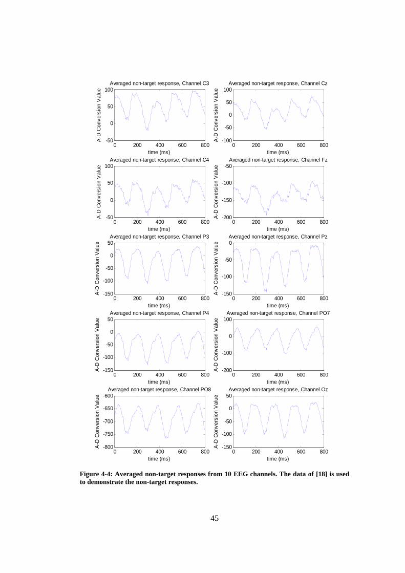
45
0 200 400 600 800-50
0
50
100Averaged non-target response, Channel C3
time (ms)
A-D
Con
vers
ion
Val
ue
0 200 400 600 800-100
-50
0
50
100Averaged non-target response, Channel Cz
time (ms)
A-D
Con
vers
ion
Val
ue0 200 400 600 800
-50
0
50
100Averaged non-target response, Channel C4
time (ms)
A-D
Con
vers
ion
Val
ue
0 200 400 600 800-200
-150
-100
-50Averaged non-target response, Channel Fz
time (ms)
A-D
Con
vers
ion
Val
ue
0 200 400 600 800-150
-100
-50
0
50Averaged non-target response, Channel P3
time (ms)
A-D
Con
vers
ion
Val
ue
0 200 400 600 800-150
-100
-50
0Averaged non-target response, Channel Pz
time (ms)
A-D
Con
vers
ion
Val
ue
0 200 400 600 800-150
-100
-50
0
50Averaged non-target response, Channel P4
time (ms)
A-D
Con
vers
ion
Val
ue
0 200 400 600 800-200
-100
0
100Averaged non-target response, Channel PO7
time (ms)
A-D
Con
vers
ion
Val
ue
0 200 400 600 800-800
-750
-700
-650
-600Averaged non-target response, Channel PO8
time (ms)
A-D
Con
vers
ion
Val
ue
0 200 400 600 800-150
-100
-50
0
50Averaged non-target response, Channel Oz
time (ms)
A-D
Con
vers
ion
Val
ue
Figure 4-4: Averaged non-target responses from 10 EEG channels. The data of [18] is used to demonstrate the non-target responses.

46
Similar to equation (4.26), the averaged non-target signal is modeled as:
∑ +=−i
iii nwBnx )sin()(targetnon φ 1,.....,1,0 −= pi (4.27)
which in this case depends only on p frequency components. Performing the
same operations described in Method 1, we obtain the Wiener filter for the non-
target system which can be represented as )(targetnon jwW − .
After all, it is desired to identify the target responses. Therefore, we will define
the final form of the filter as:
( ))(1)()( targetnontargetfinal jwWjwWjwW −−= (4.28)
Constructing the final filter as in (4.28) will enhance the target signals while
suppressing the non-target ones.
When the behavior of the noise signal is considered, it is observed to be Gaussian
distributed in this model. As an example, the histogram plots of the noise signal
for the target column and non-target row groups (at random samples of time index
n ) are given in Figure 4-5 and Figure 4-6 respectively. From these figures, it is
clear that )(nv ’s are zero-mean random processes2. This is a trivial result since
the desired signals are obtained by ensemble averaging the observations.
Therefore, subtracting the desired signal from the observations to obtain the noise
will definitely give us a zero mean signal.
2 As there are two examples (target column and non-target row groups) given to illustrate the distribution of the noise signal, and therefore two separate Wiener filter models, it is more accurate to refer the noise signal separately for each group.
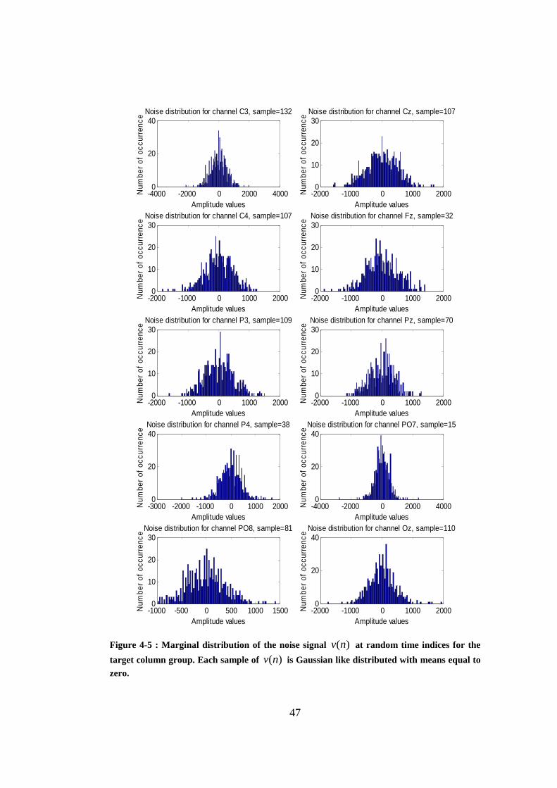
47
-4000 -2000 0 2000 40000
20
40Noise distribution for channel C3, sample=132
Num
ber
of o
ccur
renc
e
Amplitude values-2000 -1000 0 1000 20000
10
20
30Noise distribution for channel Cz, sample=107
Num
ber
of o
ccur
renc
e
Amplitude values
-2000 -1000 0 1000 20000
10
20
30Noise distribution for channel C4, sample=107
Num
ber
of o
ccur
renc
e
Amplitude values-2000 -1000 0 1000 20000
10
20
30Noise distribution for channel Fz, sample=32
Num
ber
of o
ccur
renc
eAmplitude values
-2000 -1000 0 1000 20000
10
20
30Noise distribution for channel P3, sample=109
Num
ber
of o
ccur
renc
e
Amplitude values-2000 -1000 0 1000 20000
10
20
30Noise distribution for channel Pz, sample=70
Num
ber
of o
ccur
renc
e
Amplitude values
-3000 -2000 -1000 0 1000 20000
20
40Noise distribution for channel P4, sample=38
Num
ber
of o
ccur
renc
e
Amplitude values-4000 -2000 0 2000 40000
20
40Noise distribution for channel PO7, sample=15
Num
ber
of o
ccur
renc
e
Amplitude values
-1000 -500 0 500 1000 15000
10
20
30Noise distribution for channel PO8, sample=81
Num
ber
of o
ccur
renc
e
Amplitude values-2000 -1000 0 1000 20000
20
40Noise distribution for channel Oz, sample=110
Num
ber
of o
ccur
renc
e
Amplitude values
Figure 4-5 : Marginal distribution of the noise signal )(nv at random time indices for the
target column group. Each sample of )(nv is Gaussian like distributed with means equal to zero.
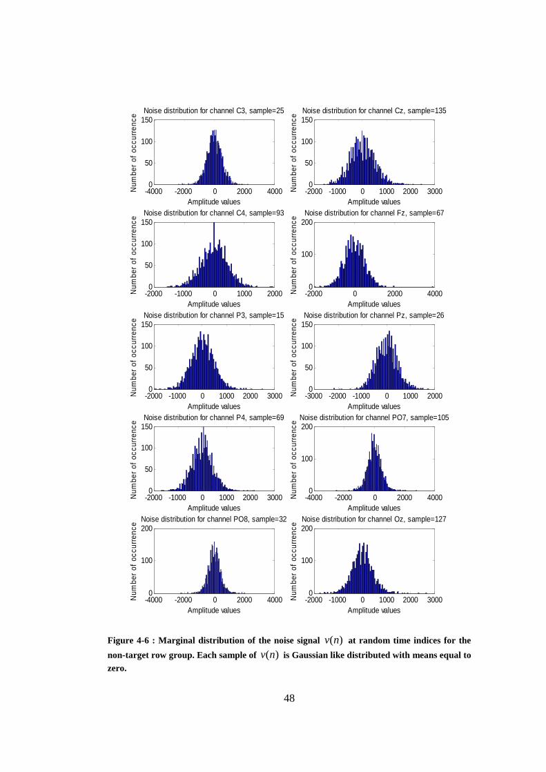
48
-4000 -2000 0 2000 40000
50
100
150Noise distribution for channel C3, sample=25
Num
ber
of o
ccur
renc
e
Amplitude values-2000 -1000 0 1000 2000 30000
50
100
150Noise distribution for channel Cz, sample=135
Num
ber
of o
ccur
renc
e
Amplitude values
-2000 -1000 0 1000 20000
50
100
150Noise distribution for channel C4, sample=93
Num
ber
of o
ccur
renc
e
Amplitude values-2000 0 2000 40000
100
200Noise distribution for channel Fz, sample=67
Num
ber
of o
ccur
renc
eAmplitude values
-2000 -1000 0 1000 2000 30000
50
100
150Noise distribution for channel P3, sample=15
Num
ber
of o
ccur
renc
e
Amplitude values-3000 -2000 -1000 0 1000 20000
50
100
150Noise distribution for channel Pz, sample=26
Num
ber
of o
ccur
renc
e
Amplitude values
-2000 -1000 0 1000 2000 30000
50
100
150Noise distribution for channel P4, sample=69
Num
ber
of o
ccur
renc
e
Amplitude values-4000 -2000 0 2000 40000
100
200Noise distribution for channel PO7, sample=105
Num
ber
of o
ccur
renc
e
Amplitude values
-4000 -2000 0 2000 40000
100
200Noise distribution for channel PO8, sample=32
Num
ber
of o
ccur
renc
e
Amplitude values-2000 -1000 0 1000 2000 30000
100
200Noise distribution for channel Oz, sample=127
Num
ber
of o
ccur
renc
e
Amplitude values
Figure 4-6 : Marginal distribution of the noise signal )(nv at random time indices for the
non-target row group. Each sample of )(nv is Gaussian like distributed with means equal to zero.
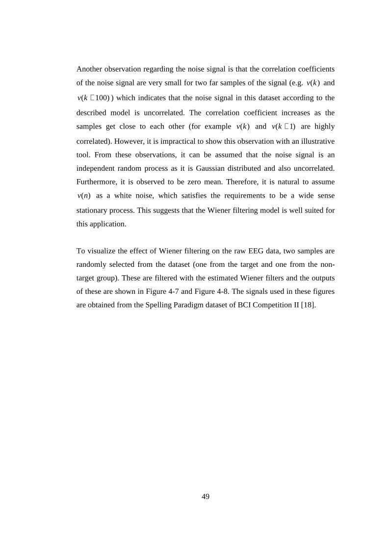
49
Another observation regarding the noise signal is that the correlation coefficients
of the noise signal are very small for two far samples of the signal (e.g. )(kv and
)100( +kv ) which indicates that the noise signal in this dataset according to the
described model is uncorrelated. The correlation coefficient increases as the
samples get close to each other (for example )(kv and )1( +kv are highly
correlated). However, it is impractical to show this observation with an illustrative
tool. From these observations, it can be assumed that the noise signal is an
independent random process as it is Gaussian distributed and also uncorrelated.
Furthermore, it is observed to be zero mean. Therefore, it is natural to assume
)(nv as a white noise, which satisfies the requirements to be a wide sense
stationary process. This suggests that the Wiener filtering model is well suited for
this application.
To visualize the effect of Wiener filtering on the raw EEG data, two samples are
randomly selected from the dataset (one from the target and one from the non-
target group). These are filtered with the estimated Wiener filters and the outputs
of these are shown in Figure 4-7 and Figure 4-8. The signals used in these figures
are obtained from the Spelling Paradigm dataset of BCI Competition II [18].
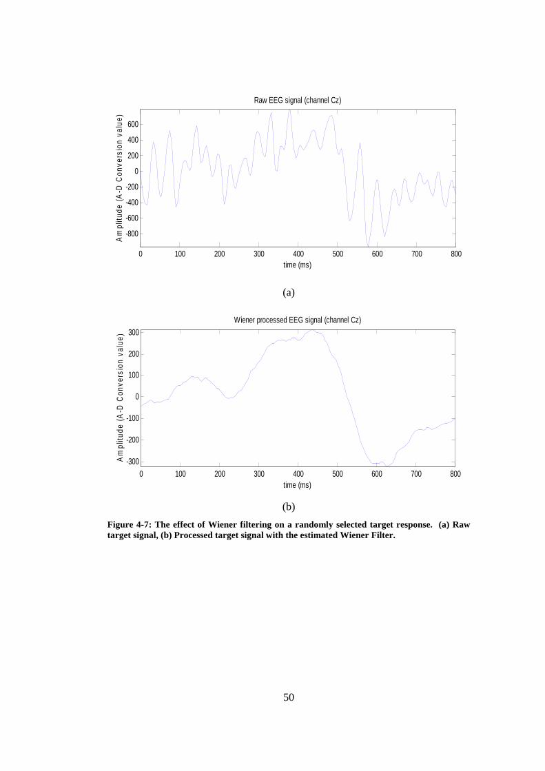
50
0 100 200 300 400 500 600 700 800
-800
-600
-400
-200
0
200
400
600
time (ms)
Am
plitu
de (
A-D
Con
vers
ion
valu
e)
Raw EEG signal (channel Cz)
(a)
0 100 200 300 400 500 600 700 800
-300
-200
-100
0
100
200
300
time (ms)
Am
plitu
de (
A-D
Con
vers
ion
valu
e)
Wiener processed EEG signal (channel Cz)
(b)
Figure 4-7: The effect of Wiener filtering on a randomly selected target response. (a) Raw target signal, (b) Processed target signal with the estimated Wiener Filter.
51
0 100 200 300 400 500 600 700 800
-500
0
500
1000
time (ms)
Am
plitu
de (
A-D
Con
vers
ion
valu
e)Raw EEG signal (channel Cz)
(a)
0 100 200 300 400 500 600 700 800
-200
-100
0
100
200
time (ms)
Am
plitu
de (
A-D
Con
vers
ion
valu
e)
Wiener processed EEG signal (channel Cz)
(b)
Figure 4-8: The effect of Wiener filtering on a randomly selected non-target response. (a) Raw non-target signal, (b) Processed non-target signal with the estimated Wiener Filter.
One can note that the amplitude of the Wiener processed target response in Figure
4-7 is comparably higher than that of Figure 4-8; the amplitude of the non-target
signal has been considerably suppressed by the filter (consider the scale of the
unfiltered signals). Moreover, the peaking time of each signal is preserved after
the filtering operation which is also important in detection of P300 responses
regarding the latency of these signals.

52
CHAPTER 5
CLASSIFICATION IN SPELLING PARADIGM
5.1 Introduction
The purpose of the BCI applications is to map the neurophysiologic signals to
basic actions, like going on a specific direction in the cursor movement
application. This mapping is performed with machine learning algorithms in
which one or more classification methods are employed to form a classification
model. The approaches in the classification methods can either be parametric or
non-parametric depending on the information supplied by the problem. However,
the common approach in BCI problems is to train the learning algorithm first
within a training phase in which the subject is asked, for example in Spelling
Paradigm, to focus on a character that is known by the algorithm. This is a
supervised learning methodology that constitutes a major topic in pattern
recognition.
In this chapter, the Spelling Paradigm will be considered in the classification
point of view. First, a short explanation will be given on supervised learning
describing the basic concepts about supervised classification. Then, the
classification methods used in this study will be described in detail. Correlations
and reference to the problem will also be given during the explanation of the
concepts.

53
5.1.1 Classification Problem in Spelling Paradigm
As discussed in Chapter 3, the prediction of the target character in P300 Speller
requires the determination of the target row and column intensifications. To
visualize the problem in the classification aspect, there are 12 classes for a 6x6
speller matrix (6 row and 6 column intensification classes). However, one can use
the intuitive idea that there are two independent groups, namely the row and
column groups as the target character should be at the intersection of only one
row and one column. Hence, there are 6 classes in each separate classification
group.
Here, the problem may seem to be a 6 class classification task at first for each
group. However, since the aim is to classify the stimulations as target or non-
target, the task is realized as a binary classification problem. The presence of one
target element out of six elements in a trial is just a constraint or a priori
information supplied by the problem.
As discussed in chapter 2, the population of the non-target class should be higher
than that of the target one in order to present a well behaved P300 pattern. If this
case is considered in Bayesian classification point of view (see section 5.4.1), the
probability of each stimulus to be the target character is 1/6. When one applies
the Bayes decision rule for this problem, all new coming test samples will be
assigned to the non-target class which provides a classification accuracy of 5/6 for
each of the row and column groups. However, in this problem, the employed
classification methods should determine at least one stimulus as from the target
class for each trial. Therefore, the classification of these classes is usually
performed using supervised learning techniques which will be discussed in the
next section.

54
5.2 Supervised Learning
Most of the classification algorithms deal with a group of data that has some
information about the dataset. In other words, the class label information is given
within the dataset for training the classifier. This type of classification belongs to
supervised learning, in which a supervisor instructs the classifier during the
construction of the classification model. Linear Discriminant Functions (LDF),
Support Vector Machines (SVM’s) and Neural Networks (NN) are some well-
known examples of supervised learning and commonly used in many
classification problems.
In the supervised learning approach, there are pairs of examples in the given
training dataset which can be mathematically expressed as
( ) ( ) ( ){ }NN yxyxyxD ,,,.........,,, 2211= . Here, Nxxx ...,,........., 21 are the
observations and Nyyy ...,,........., 21 are the class labels of the observations. The
observations can be any vector, whose elements are selected from a set of features
(section 5.2.3). But for practical considerations, we usually have real valued
observations and it is easy to assume MRXx =∈ . Also, one can choose any type
of representation for the class labels. For simplicity, they are usually represented
as real numbers, that is RYy =∈ . Therefore, in supervised learning, the aim is to
find the transformation between the feature space X and the class label space Y ,
i.e. YXf →: . If the class space has a finite number of elements, i.e.
}...,,.........2,1{ Ly∈ then the problem is considered as a classification task. On the
other hand, if there are infinite classes, then the case becomes a regression
problem. For the case of Spelling Paradigm, it is a binary classification problem
in which the classes are the target and nontarget classes. For clarity and
conformity with the literature, these classes are represented as }1,1{ +−=Y where
the negativity represents the nontarget case.
55
For such a problem, additional parameters underlying the classification rule can
also be given such as the probabilistic distribution, or the form of the density
function of the classes. When this is the case, the transformation of the
observations to the class labels takes the form of ),( θxfy = . Whether these are
provided or not, one can estimate the parameters or unknown densities of the class
conditional probabilities by employing parametric or nonparametric estimation
techniques. However, these will not be explained in this context. The reader can
find detailed information about the estimation in supervised learning in [34].
5.2.1 Linear Discriminant Functions
A type of supervised learning called Linear Discriminant Functions (LDF) will be
considered as a motivation to Support Vector Machine (SVM) which is used as
the main classification method in Spelling Paradigm [77]. The importance of LDF
is that they form the base of many discriminative classification methods and
constitute a major subject in classification literature. It is a non-parametric
supervised learning in which the form of the discriminating function is known or
assumed instead of the probabilistic distribution of the classes. The form of the
discriminating function may not essentially be linear in the feature vector;
however, linearity brings additional properties that provide some advantages in
analytical point of view [34]. Also, being easier to implement, LDF provide a well
understandability of the discriminant classification with a simple model.
It is easy to demonstrate LDF in a two class case where the classes are also
linearly separable as shown in Figure 5-1. The aim in LDF is to construct a
hyperplane, or mathematically, to find the parameters defining the hyperplane that
separates two classes by using the samples in the training dataset.
So, a linear discriminant function can be expressed in terms of the feature vector
x as
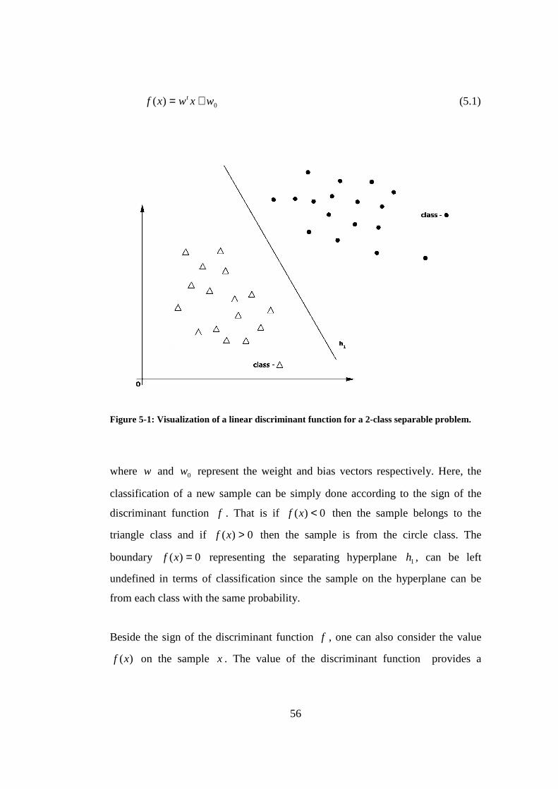
56
0)( wxwxf t += (5.1)
Figure 5-1: Visualization of a linear discriminant function for a 2-class separable problem.
where w and 0w represent the weight and bias vectors respectively. Here, the
classification of a new sample can be simply done according to the sign of the
discriminant function f . That is if 0)( <xf then the sample belongs to the
triangle class and if 0)( >xf then the sample is from the circle class. The
boundary 0)( =xf representing the separating hyperplane 1h , can be left
undefined in terms of classification since the sample on the hyperplane can be
from each class with the same probability.
Beside the sign of the discriminant function f , one can also consider the value
)(xf on the sample x . The value of the discriminant function provides a

57
measure of distance between the sample and the separating hyperplane. This can
be seen if one uses the following expression for x :
{ w
wd
xxwx
p
t += (5.2)
where px and d represent the projection of the sample x on the hyperplane 1h
and distance of the sample to the hyperplane respectively. This distance is
illustrated in Figure 5-2.
Figure 5-2: Relation between the function value of the sample x and its distance to the discriminating hyperplane.

58
Without going into detail, the distance d gives an idea of the probability value of
the sample being in that halfspace. Although this is not always true, the larger
value of d can be assumed to be the higher probability of right decision.
5.2.2 Error and Risk in Classification
Due to the stochastic nature of the problems, the error or the misclassification of
samples is inevitable in pattern recognition. In fact, the principle of the
classification methods is to minimize the error in classification or the risk in the
decision. In this section, it is aimed to describe these concepts which are
mentioned throughout following sections of this chapter. The explanations will be
restricted to the binary classification problem which is the case in Spelling
Paradigm. The reader can find detailed explanation for multiclass case in [34],
and [35].
To begin with the error in classification, consider the Bayesian case where the
decision is made according to the class conditional probabilities (discussed in
section 5.4.1). That is, classify x as 1C if )()( 21 xCPxCP > or vice versa. In this
case, one can not think of the error itself only, but the average probability of error
which can be expressed as:
),(),()( 2112 CRxPCRxPeP ∈+∈= (5.3)
where 1R and 2R represent the halfspaces separated by the decision surface.
Applying the Bayes Theorem on (5.3) yields:
∫∫ +=
∈+∈=
12
)()()()(
)()()()()(
2211
221112
RR
dxCPCxpdxCPCxp
CPCRxPCPCRxPeP (5.4)

59
which is also known as expected error or error rate and it is minimized by the
Bayes decision rule stated above [34], [35].
Beside the average probability of error, one can also consider the risk in taking
the decision in the problem. For example, in the P300 Speller case the risk of
deciding the sample as target can be higher than the risk of deciding the sample as
nontarget. Therefore, the risk or expected loss for taking an action iα can be
defined in a two class problem as follows:
∑ ∫=
=2
1
)()()(j R
ijii dxCxpCxRj
αλα (5.5)
In this scope, a loss function (.)λ is introduced in the problem which is usually
defined for two class case as:
2,1,,1
,0),( =
≠=
= jiji
jiC jiαλ (5.6)
In this loss function, the cost of wrong decision in each class is equal. However,
one can also define the loss function according to the nature of the classification
problem. When defined as in this case, one can show that overall expected loss or
risk becomes identical to the average probability of error defined in (5.4).
dxCPCxpdxCPCxp
CPxRR
RR
iii
∫∫
∑
+=
==
12
)()()()(
)()(
2211
2
1
α (5.7)
However, the conditional probability densities are not always known in
supervised learning methods like discriminant functions or SVM. The only
information provided in supervised learning is a training dataset which includes

60
the class labels. Therefore, the evaluation and minimization of the risk is not
possible by using the expressions above. Instead, one can employ empirical risk
minimization to construct the discrimination function by using the training
samples in the given dataset. The empirical risk in supervised learning is defined
as follows:
[ ] ( )∑=
=N
jjjemp xfy
NfR
1
)(,1 λ (5.8)
And the optimum discriminant function is the one which minimizes the empirical
risk.
[ ]
=∈
fRxf empHf n
minarg)(ˆ (5.9)
where nH is the function space of interest.
One should note that the empirical risk makes sense only if it is equal to the
expected risk if the number of elements in the training set goes to infinity. That is,
[ ] RfRempN
=∞→
lim (5.10)
When this is not true, one can encounter some problems which will be mentioned
in the next section.
5.2.3 Feature Space
The data given for training and testing the classifier are usually gathered from a
recording device and contain raw data information. However, one can use some of
the elements for classification instead of all from the supplied information. The
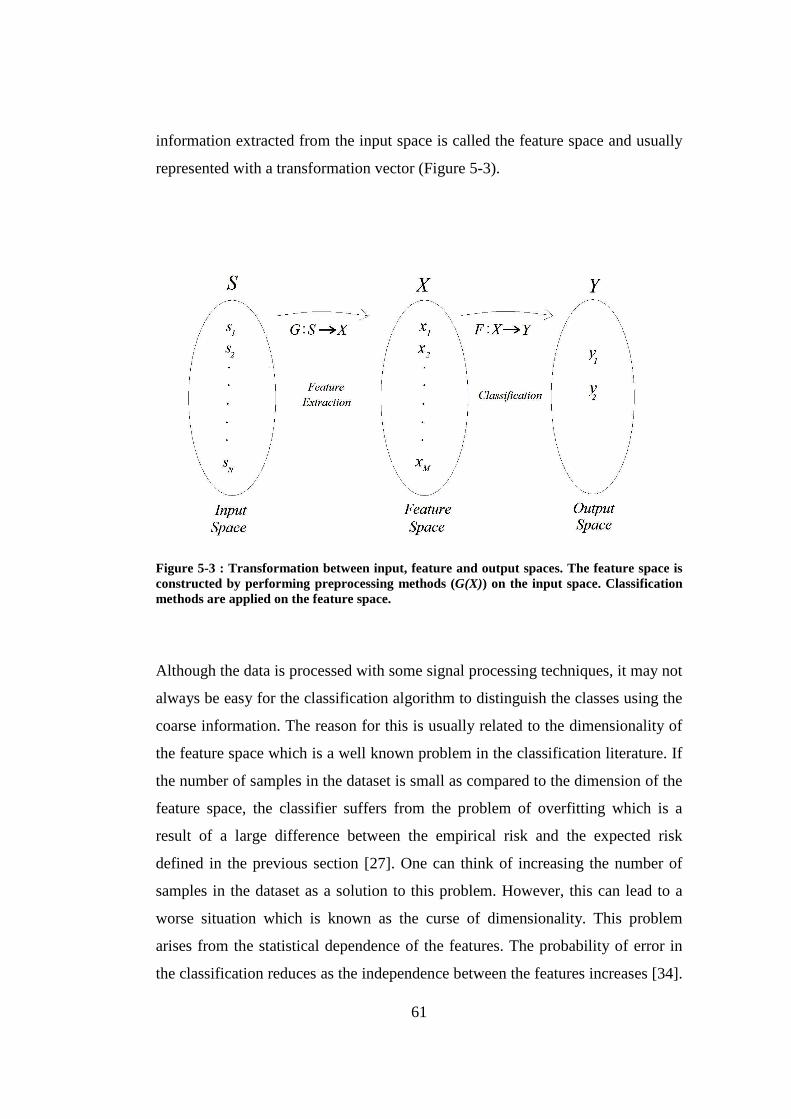
61
information extracted from the input space is called the feature space and usually
represented with a transformation vector (Figure 5-3).
Figure 5-3 : Transformation between input, feature and output spaces. The feature space is constructed by performing preprocessing methods (G(X)) on the input space. Classification methods are applied on the feature space.
Although the data is processed with some signal processing techniques, it may not
always be easy for the classification algorithm to distinguish the classes using the
coarse information. The reason for this is usually related to the dimensionality of
the feature space which is a well known problem in the classification literature. If
the number of samples in the dataset is small as compared to the dimension of the
feature space, the classifier suffers from the problem of overfitting which is a
result of a large difference between the empirical risk and the expected risk
defined in the previous section [27]. One can think of increasing the number of
samples in the dataset as a solution to this problem. However, this can lead to a
worse situation which is known as the curse of dimensionality. This problem
arises from the statistical dependence of the features. The probability of error in
the classification reduces as the independence between the features increases [34].

62
But when the features are statistically dependent, the classification performance is
limited and can not be improved by adding new features.
A solution to this problem is to use other properties of the data by applying
feature selection. For example, in a BCI problem, the band power of the EEG
signal or coefficients of the autoregressive parameters might contain more useful
information for the classifier than the signal itself in a mu-rhythm based BCI. As
stated in chapter 3, there are also feature extraction algorithms that automatically
select the elements for the feature space which improve the classification
performance. However, in this study, due to the computational simplicity and
conformity with the literature, the features are selected manually without any
feature extraction method. As in [4], we have used the EEG time segments of 600
or 800 ms duration after the stimulus onset from the electrode locations Fz, Cz,
Pz, Oz, C3, C4, P3, P4, PO7 and PO8 (Figure 7-3 (a)) and set the Wiener filtered
signals as our feature vector. The dimension of the feature vector varies according
to the sampling rate of the EEG recording device. For illustration purposes, the
Wiener filtered EEG signals are concetanated by channel to form the feature
vector as seen in Figure 5-4.
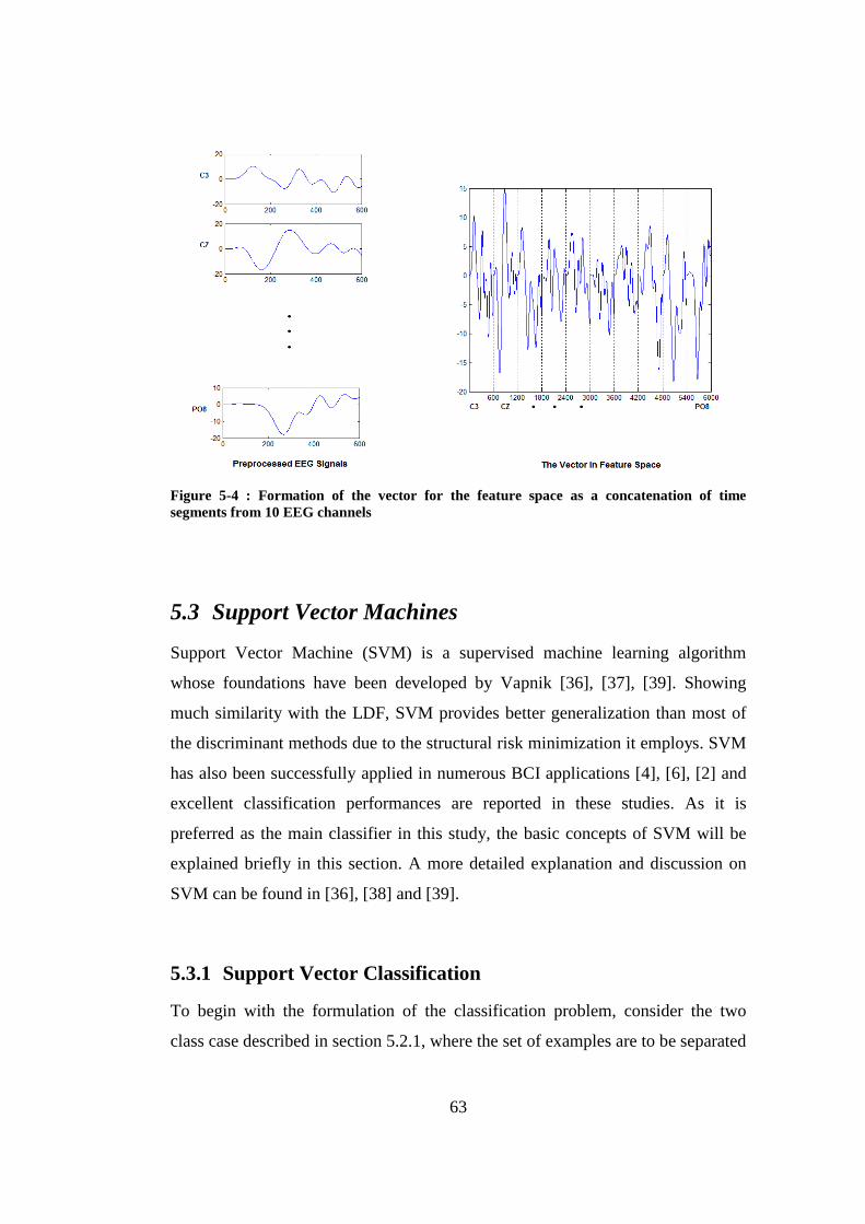
63
Figure 5-4 : Formation of the vector for the feature space as a concatenation of time segments from 10 EEG channels
5.3 Support Vector Machines
Support Vector Machine (SVM) is a supervised machine learning algorithm
whose foundations have been developed by Vapnik [36], [37], [39]. Showing
much similarity with the LDF, SVM provides better generalization than most of
the discriminant methods due to the structural risk minimization it employs. SVM
has also been successfully applied in numerous BCI applications [4], [6], [2] and
excellent classification performances are reported in these studies. As it is
preferred as the main classifier in this study, the basic concepts of SVM will be
explained briefly in this section. A more detailed explanation and discussion on
SVM can be found in [36], [38] and [39].
5.3.1 Support Vector Classification
To begin with the formulation of the classification problem, consider the two
class case described in section 5.2.1, where the set of examples are to be separated
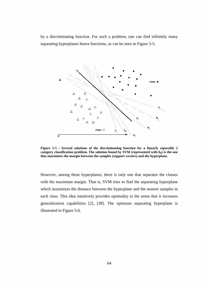
64
by a discriminating function. For such a problem, one can find infinitely many
separating hyperplanes hence functions, as can be seen in Figure 5-5.
Figure 5-5 : Several solutions of the discriminating function for a linearly separable 2 category classification problem. The solution found by SVM (represented with h0) is the one that maximizes the margin between the samples (support vectors) and the hyperplane.
However, among these hyperplanes, there is only one that separates the classes
with the maximum margin. That is, SVM tries to find the separating hyperplane
which maximizes the distance between the hyperplane and the nearest samples in
each class. This idea intuitively provides optimality in the sense that it increases
generalization capabilities [2], [38]. The optimum separating hyperplane is
illustrated in Figure 5-6.
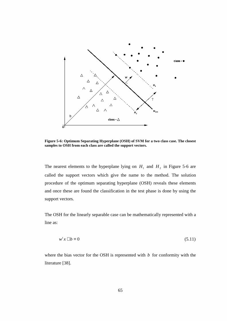
65
Figure 5-6: Optimum Separating Hyperplane (OSH) of SVM for a two class case. The closest samples to OSH from each class are called the support vectors.
The nearest elements to the hyperplane lying on 1H and 2H in Figure 5-6 are
called the support vectors which give the name to the method. The solution
procedure of the optimum separating hyperplane (OSH) reveals these elements
and once these are found the classification in the test phase is done by using the
support vectors.
The OSH for the linearly separable case can be mathematically represented with a
line as:
0=+ bxwt (5.11)
where the bias vector for the OSH is represented with b for conformity with the
literature [38].

66
The solution for OSH requires the solution of an optimization problem where the
goal is to maximize the margin γ . Here, if one sets the class labels as { }1,1−=y ,
then 1)( ≥+ bxwy it
i becomes a constraint of this optimization problem. This
constraint comes from the restriction that
1)(min =+ bxw it
i (5.12)
which simplifies the formulations in the problem. With these constraints one can
show that the margin γ is related to the weight vector w with:
w
2=γ (5.13)
Therefore, maximizing the margin γ is equivalent to minimizing the norm of the
weight vector. So the quadratic support vector optimization problem is formulated
as follows:
Nibxwyts
w
it
i ,,.........2,11)(..2
1minimize
2
=≥+ (5.14)
where N is the number of elements in the training set.
SVM can find the optimum solution for the separating hyperplane from (5.14)
only if the classes are linearly separable. However, this is not usually the case. In
real problems the data is inseparable even with the feature extraction methods and
higher dimension mappings which will be discussed in the later sections of this
chapter. To overcome this problem, (5.14) is modified by introducing a penalty
function and positive slack variables into the optimization problem [39], [38]:

67
i
Nibxwyts
Cw
i
iit
i
N
ii
∀>=−≥+
+ ∑
0
,,.........2,11)(..
2
1minimize
2
ξξ
ξ
(5.15)
where iξ ’s are the slack variables and C is the regularization parameter. This
modification provides a more flexible situation which is named as the “soft-
margin” SVM optimization problem [4]. The iξ parameters moderate the
constraints by allowing violations and provide the penalty together with the
regularization parameter in the cost function.
The solution for the optimum separating hyperplane is simplified when the cost
function in (5.15) is expressed in the Lagrangian dual form:
∑
∑∑
=≤≤
−≡
iii
i
jij
tijiji
iiD
ya
Cats
xxyyaaaL
0
0..
2
1maximize
,
(5.16)
This formulation provides an advantage that one does not deal with the slack
variables inside the cost function. One should also note that the solution is found
in terms of the Lagrange multipliers ia for all the training points ix and the non-
zero solutions for ia ’s represent the coefficients of the support vectors. Therefore,
the solution for the weight vector w of the OSH is found from:
∑=sN
iiii xyaw (5.17)
where ix ’s and sN represent the support vectors and the number of the support
vectors respectively.

68
The solution for the threshold or the bias term b can be found from the Karush-
Kuhn-Tucker (KKT) conditions for the primal Lagrangian form which states
( )[ ] ibwxya tiii ∀=−+ ,01 (5.18)
Expression (5.18) is, in fact, a simplified case of the real KKT conditions. The
slack variables iξ ’s are removed here by using the fact that Cai <<0 . This
constraint implies that 0=iξ when the Lagrange multipliers are in this range.
Therefore, from (5.18) one can use all the training points to compute the bias term
b for which Cai <<0 is satisfied. As there are at most N equations in (5.18)
one may find N different solutions for b and the common approach is to average
all these solutions to compute the bias vector [38].
5.3.2 Prediction in SVM
When the parameters defining the OSH are found, the class labels of the new
coming vectors are determined by evaluating the sign of the function defined in
(5.19).
bxwxf t +=)( (5.19)
The function is expressed in terms of the support vectors if the equation (5.19) is
combined with (5.17) as:
∑ +=sN
ii
tii bxxayxf )( (5.20)

69
The sign of the function value indicates the side of the OSH on which the vector
lies and the absolute value of the function gives the idea of distance of the vector
to the hyperplane. In other words, the higher the absolute value of the function,
the higher the probability of the vector being in that halfspace.
5.3.3 Kernel Functions
Up to here, SVM is discussed in the linear functions of the data, i.e. the
discriminating function used in classification is a linear transformation of the
feature vector to the output space. The Kernel operator used in the above SVM
discussions is the usual dot product of the two vectors. However, one can also
employ other transformations to generalize the SVM to the nonlinear case. The
idea is to map the vectors into a higher dimensional space which provides some
advantages in cases where the data is linearly inseparable [38]. So, one can
express the Kernel operation as an inner product in the feature space as:
)(),(),( jiji xxxxK ΦΦ= (5.21)
where the operation .,. represents the inner product and the function (.)Φ
provides the nonlinearity in the transformation of the feature vector. Therefore,
the inner product in SVM discriminant function can be replaced by the
generalized Kernel operator defined in (5.21).
( )∑ +=sN
iiii bxxKayxf ,)( (5.22)
Some examples of the nonlinear Kernel functions used in SVM are defined in the
following:

70
• Polynomial Kernel:
d
jiji xxxxK ,),( = (5.23)
or
( )d
jiji xxxxK 1,),( += (5.24)
• Gaussian Radial Basis Function:
2
2
2),( σji xx
ji exxK
−−
= (5.25)
• Exponential Radial Basis Function:
22),( σji xx
ji exxK−
−= (5.26)
• Dirichlet Kernel:
( )
−
−
+=
2sin2
2
1sin
),(ji
ji
ji xx
xxN
xxK (5.27)
• Sigmoid Function:
( )δκ −= jiji xxxxK .tanh),( (5.28)
Among these kernel operators, the Gaussian Radial Basis Function (Gaussian
RBF) is reported to provide excellent results in the classification and
generalization performance of SVM as compared to other functions [40], [38].

71
The variance expression 2σ in Gaussian RBF provides an additional control
parameter that leads to a more suitable decision boundary for many classification
problems. Also in BCI studies, the Gaussian RBF is preferred in SVM due to its
success in classification [4], [2].
5.3.4 Normalization
Normalization is a data processing technique used in statistics, signal processing
and machine learning applications. It is used to standardize the magnitude or
decrease the variance of the elements in the set of interest. For classification point
of view, the samples in a training set usually exhibit a large variance. It is
sometimes necessary for removing the extremity of the samples and increasing
the correlations between the samples from the same class when training the
classifier.
There are several techniques for data normalization. The simplest one is to
normalize the length or the magnitude of the vector; that is the normalized sample
is equal to the unit vector pointing in the direction of the input sample.
x
xx =)
(5.29)
The norm operation in (5.29) is the 2L norm which corresponds to the linear
scaling of the input vector with its magnitude. There are also other normalization
options like scaling the input vector with the difference between the maximum
and minimum of the input vector:
)min()max(
)min(
xx
xxx
−−=)
(5.30)

72
In (5.30), the input vector is linearly scaled to the interval [ ]1,0 . This range can be
modified according to the requirements of the classifier (if exists any) as:
( ) )min()min()min()max(
)min()max(xxx
xx
xxx
)))
) +−−−= (5.31)
Up to here, the normalization is explained by using only the properties of a single
sample in the dataset. However, one can also employ ensemble normalization
which is performed over the whole dataset. In this approach, the statistical
properties of the dataset such as the means or the variances of the features are
used to scale the samples. A well known type of ensemble normalization is the
Gaussian normalization in which all the features are normalized with according to
a normal distribution ( )σµ,N .
2x
xxx
σµ−
=) (5.32)
where xµ and 2xσ represent the mean and variance vectors of the features
respectively.
5.3.5 Cross-Validation
Cross-validation is a testing method in supervised learning used for assessing the
generalization performance of a classification model. The idea is to divide the
training set into small partitions and use only one partition to train the classifier.
The remaining subsets (validation set) are left to test the classifier where the result
of classification could be justified. The cross-validation is performed by rotating
the subsets used for training and the result of the prediction accuracy over the
validation set is averaged for all combinations. Application of this technique
allows the modification of the parameters that are used to construct the classifier
and thus provides a generalization procedure for the classifier.

73
Two types of the cross-validation are commonly used in measuring the accuracy
of the classification model which are the random sub-sampling and κ - fold cross-
validation methods. In random sub-sampling cross-validation, the training set is
randomly partitioned into training and validation sets and the classification model
is tested on the validation set for each partitioning operation. The averaging is
performed over the partitions to determine the average accuracy of the model. On
the other hand, the κ - fold cross-validation divides the training set into κ
subsets. The classifier is trained on 1−κ of these subsets and then tested on the
remaining subset. This operation is then repeated for κ times until all the subsets
are used as a validation set for the classifier. The κ classification accuracy results
obtained from the validation sets are then averaged to asses the overall
performance of the classifier. In this study, the κ -fold cross-validation method is
preferred for the comparison of the classifier performance with the results given
in [4]. It is used to determine the optimal control parameters which are the
regularization parameter in the penalty function of SVM defined in (5.15) and
variance parameter of the Gaussian RBF kernel in (5.25).
5.4 Unsupervised Learning
The supervised learning techniques like SVM employ only the data to construct
the classification model and the additional information supplied by the problem is
not used in these methods. As described in section 5.1.1, for the case of Spelling
Paradigm, the information given by the problem is that there exists only one target
class in each of the row and column groups for a single trial. Discriminant
classification, on the other hand, can decide as if there are multiple target classes
in each group which is not true for the Spelling Paradigm case. For example, the
classifier can predict two or more rows from the same trial as the target class or
all columns as the nontarget class. To overcome this problem, unsupervised
learning techniques are involved by using the probabilistic information supplied
by the problem. Therefore, in this section, the Bayesian classification together

74
with the Maximum Likelihood Estimation (MLE) will be explained as the
unsupervised learning technique in Spelling Paradigm.
5.4.1 Bayesian Classification
The Bayesian classification is the simplest machine learning technique that
employs the a posteriori probabilities of the observations in the decision. It is used
in both supervised and unsupervised learning depending on the information
provided by the problem. In this section, Bayesian decision is explained for
unsupervised learning in which only the state conditional probability density of
the observations and the a priori probabilities of the classes are known.
To begin with the Bayes decision theory, classification for an observation x is
done according to the Bayes Rule which is defined as:
( ) ( ) ( ))(xp
CPCxpxCP
jj
j = (5.33)
Here, ( )xCP j represents the a posteriori probability of x for the class jC . In
other words, it is the probability of an observation belonging to that class. It can
be interpreted for the Spelling Paradigm case as the true probability of a row or
column being from the target or non-target class once it is observed. Moreover,
( )jCxp is the class-conditional probability density of x for the j -th class which
represents the distribution of x when the j -th class is observed. This can be
interpreted as the probability of a row or column once it is decided (by the SVM
classifier) as from the target or nontarget class.
If the case is restricted to the two class case, one can express the probability
density of x in (5.33) as:

75
( ) )()(2
1j
jj CPCxpxp ∑
== (5.34)
The Bayesian decision is performed according to the intuitive idea that if
( ) ( )xCPxCP ij > then the observation x belongs to the j -th class and this
minimizes the risk in classification as discussed in section 5.2.2. Once the class-
conditional densities are known, the Bayesian classification can be applied for
prediction of the observations using the rule defined in (5.33). If the probability
densities are unknown or depend on some parameters, then parameter estimation
techniques can be applied to determine the distribution of the class-conditional
probabilities. A common parameter estimation technique, known as the Maximum
Likelihood Estimation (MLE) will be the topic of the next section.
5.4.2 Maximum Likelihood Estimation
Maximum Likelihood Estimation (MLE) is used in cases where the conditional
probability density function is unknown, but the form of the function is known.
The conditional probability in this case depends on some parameters
( )Nθθθθ ,....,, 21= such as mean or variance of the distribution, and these
parameters can be estimated using the MLE method. For the case of Spelling
Paradigm, the unknown parameter θ will represent the trial dependency of the
target class prediction. Here, the MLE is discussed on the estimation of the
conditional probability density ( )jCxp required in the Bayesian classifier.
To begin with, the dependence of the class-conditional probability density
( )jCxp to the unknown parameter θ can be expressed in a joint density as
( )θ,jCxp . For our case, ( )θ,jCxp represents the class-conditional probability
density for each trial repetition. Since the form of ( )θ,jCxp is known (it can be

76
observed from each trial), the best estimate of the class-conditional density
( )jCxp is obtained by averaging3 ( )θ,jCxp over θ [34]:
( ) ( )∫= ", θθ dCxpCxp jj (5.35)
The expression (5.35) in fact, provides the MLE of the class-conditional density
provided by the SVM outputs for the spelled character. Kaper et al. considered
this case as the scoring of the row and column intensifications regarding the SVM
outputs [4] but did not formulate the problem in a probabilistic methodology.
At this point, one can think of a better estimation of ( )jCxp for a real world
problem in P300 Speller. For example, consider the case that the subject wants to
stop the spelling application and rest for a moment. In other words, he/she refuses
to spell a character. In this case, a stopping criteria should be introduced into the
problem. Therefore, one can modify the decision rule in prediction as follows:
3 The expression ( )Xp θ in [34] has been omitted here as it is obvious that it is equal to 1 for the
P300 Speller (There is always a trial for any observation). However, for an online system in which the subject may not always desire to perform spelling, the form of the conditional density
( )Xp θ should be considered.
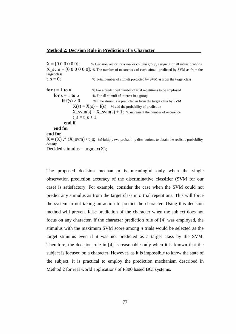
77
Method 2: Decision Rule in Prediction of a Character
X = [0 0 0 0 0 0]; % Decision vector for a row or column group, assign 0 for all intensifications X_svm = [0 0 0 0 0 0]; % The number of occurences of each stimuli predicted by SVM as from the target class t_s = 0; % Total number of stimuli predicted by SVM as from the target class for t = 1 to n % For a predefined number of trial repetitions to be employed
for s = 1 to 6 % For all stimuli of interest in a group
if f(s) > 0 %if the stimulus is predicted as from the target class by SVM X(s) = X(s) + f(s) % add the probability of prediction
X_svm(s) = X_svm(s) + 1; % increment the number of occurence t_s = t_s + 1; end if end for end for X = (X) .* (X_svm) / t_s; %Multiply two probability distributions to obtain the realistic probability density Decided stimulus = argmax(X);
The proposed decision mechanism is meaningful only when the single
observation prediction accuracy of the discriminative classifier (SVM for our
case) is satisfactory. For example, consider the case when the SVM could not
predict any stimulus as from the target class in n trial repetitions. This will force
the system in not taking an action to predict the character. Using this decision
method will prevent false prediction of the character when the subject does not
focus on any character. If the character prediction rule of [4] was employed, the
stimulus with the maximum SVM score among n trials would be selected as the
target stimulus even if it was not predicted as a target class by the SVM.
Therefore, the decision rule in [4] is reasonable only when it is known that the
subject is focused on a character. However, as it is impossible to know the state of
the subject, it is practical to employ the prediction mechanism described in
Method 2 for real world applications of P300 based BCI systems.

78
CHAPTER 6
THE DESIGN OF ELECTROENCEPHALOGRAPHIC
DATA ACQUISITION SYSTEM FOR BCI
APPLICATIONS
6.1 Introduction
Beside the signal processing techniques and classification methods, the
mechanisms in measurement of the brain activity and decision in experimental
paradigms are of quite importance. The quality of the signal detecting and
recording devices considerably affect the performance of the BCI algorithms. As
mentioned in Chapter 2, BCI systems usually use electroencephalogram to
measure the brain activity due to its portability and practicality. In this chapter,
we will present a prototype design of an EEG system to be used BCI applications.
The design of the system mainly covers the design of an EEG amplifier, the data
acquisition hardware, electrode and EEG cap designs and the software controller
design for BCI experiments. Here, in this chapter, the designed system is
explained briefly. Detailed information (system diagrams, performance tests etc.)
can be found in the technical documentation of the EEG system [82].

79
6.1.1 EEG Design Requirements
• EEG systems are used in medical applications. They should first satisfy some
safety requirements in order not to harm the subject. Therefore, electrical
safety should be of primary consideration; isolations from the power network
should be implemented properly.
• As stated in Chapter 2, the amplitude of EEG signals is on the order of several
microvolts (~ Vµ100 ). Therefore, the system should be capable of sensing the
signals in this range. The gain of the amplifier system and the resolution of the
analog to digital conversion should be taken into account.
• Since the signal amplitudes are very low, EEG systems are usually affected
from noise, especially from the noise of the power network and the digital
circuitry. The filters should reduce the noisy effects of the signals that are not
related to EEG. The analog and digital grounds should be isolated properly.
• EEG signals cover a small frequency range in BCI applications. The system
should sense the electrical activity of the brain for frequencies lower than
40Hz.
• Sampling rate should be high enough considering the EEG frequency range
(Table 2-1).
• For the P300 based BCI applications like Spelling Paradigm, the system
should support recording the epoch information synchronously with the
signal.
• Regarding the previous studies performed on spelling paradigm, there should
be at least 10 channels in the system [4].
• The system should be implemented with minimum number of hardware
components.

80
6.2 System Specifications
The system design is performed according to the needs listed in the previous
section. Basically, the system is designed satisfying the following specifications:
• The analog amplifier circuitry will be supplied by standard batteries in order
to reduce the effect of noise caused by the mains supply. Also, the batteries
are preferred due to electrical safety issues.
• Active electrodes will be used in the system.
• The amplifier system will be AC-coupled in order to eliminate the DC offsets.
• EEG measurements will be monopolar.
• The isolation between the analog and digital circuitries will be performed with
analog isolators.
• ADC resolution is chosen as 12 bits.
• The digital data will be transferred to PC via USB.

81
6.3 Analog Hardware
The analog hardware is composed of an active electrode stage and an amplifier
circuitry which mainly includes instrumentation amplifiers, filters and isolator
components inside. These will be explained in detail in the following subsections.
The circuit diagrams of the system can be found in Appendix B.
6.3.1 Active Electrodes
Instead of simple passive ring electrodes, in this design, the use of active
electrodes is preferred due to their practicality. When using the passive electrodes
in EEG, a preparation stage is needed in which the electrodes have to be covered
with a conductive gel. This is a time consuming procedure especially when the
number of the electrodes is high. Moreover, the conductive paste usually dries out
after 2-3 hours of use and additional pasting is needed in order to continue to EEG
recording. Active electrodes eliminate the need for pasting and thus can be used
for the measurements much longer than the passive ones.
As EEG signals are very low amplitude signals, they are more prone to noise.
Also, for the passive electrodes, it is difficult to match the contact impedance
between the scalp and the electrode leads for all channels. This results in the
amplification of the displacement currents in the preamplifier stage [83]. The
active electrodes are usually used as voltage follower devices to improve the
signal strength at the scalp by increasing the current driving capability of the
signal. There are also studies on the design of active electrodes with gain.
However, it is difficult to overcome the problem of DC offsets in EEG. Therefore,
in this study, it is preferred to use active electrodes as simple voltage buffering
elements. Additionally, a first order high pass filter with a low cutoff frequency is
used to remove the DC component in the signal in order not to saturate the
preamplifier. Figure 6-1 shows the simulations on frequency characteristics of the
designed active electrodes.
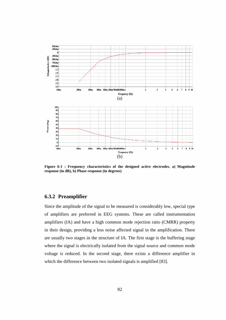
82
(a)
(b)
Figure 6-1 : Frequency characteristics of the designed active electrodes. a) Magnitude response (in dB), b) Phase response (in degrees)
6.3.2 Preamplifier
Since the amplitude of the signal to be measured is considerably low, special type
of amplifiers are preferred in EEG systems. These are called instrumentation
amplifiers (IA) and have a high common mode rejection ratio (CMRR) property
in their design, providing a less noise affected signal in the amplification. There
are usually two stages in the structure of IA. The first stage is the buffering stage
where the signal is electrically isolated from the signal source and common mode
voltage is reduced. In the second stage, there exists a difference amplifier in
which the difference between two isolated signals is amplified [83].
83
Since instrumentation amplifier includes at least three operational amplifiers (op-
amp) in its design, it occupies a larger size compared to other components in the
circuits. However, there are also commercial instrumentation amplifiers that
provide all the components in an instrumentation amplifier in a single package.
These packages have comparatively smaller size and provide the gain adjustment
with a single external resistor.
In this design, the commercial instrumentation amplifier package, LT1167 of
Linear Technologies is used at the preamplifier stage which was also employed in
the design of the 256 channel EEG system in [78]. For the elimination of high
frequency signals, first order low pass filters are added to the inputs. Moreover, a
high pass filter is used for AC coupling at the output of the amplifier.
6.3.3 Active Filters
Noise is the major problem in biopotential measurement devices. Especially, the
noise caused by the power network affects these devices by imposing a common
mode signal on the inputs of the amplifier blocks. Therefore, the need for filter
use is inevitable in these systems.
In BCI applications, the algorithms use the frequency band between 0.1Hz and
45Hz. Signals out of this range should be removed by including either analog or
digital filters in the design. Also, application of filters can solve possible aliasing
problems in digitizing circuitry. Therefore, in this design, two active filters are
used in the EEG amplifier circuitry: the first one is a band-stop filter to remove
the effect of noise caused by the mains supply and the second one is a third order
low pass Bessel filter with cutoff frequency 40Hz. The choice of Bessel filter is
due to the flat group delay response in the pass band. The magnitude and phase
response plots of these filters are given Figure 6-2 and Figure 6-3.
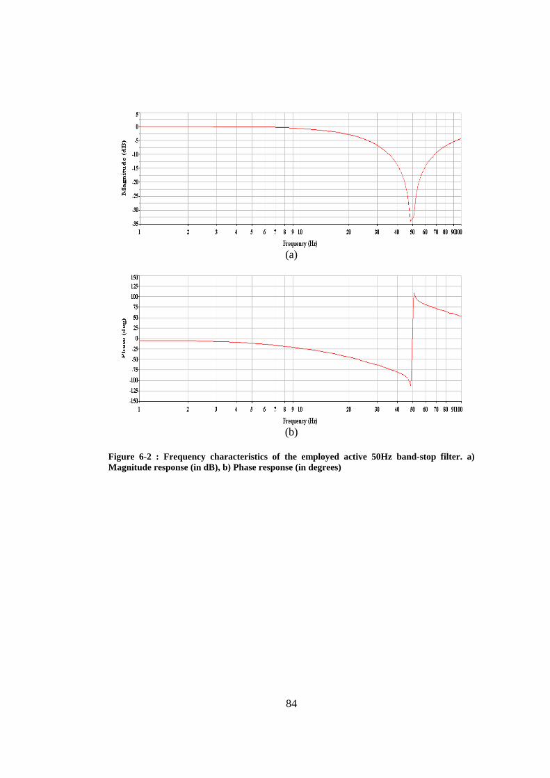
84
(a)
(b)
Figure 6-2 : Frequency characteristics of the employed active 50Hz band-stop filter. a) Magnitude response (in dB), b) Phase response (in degrees)
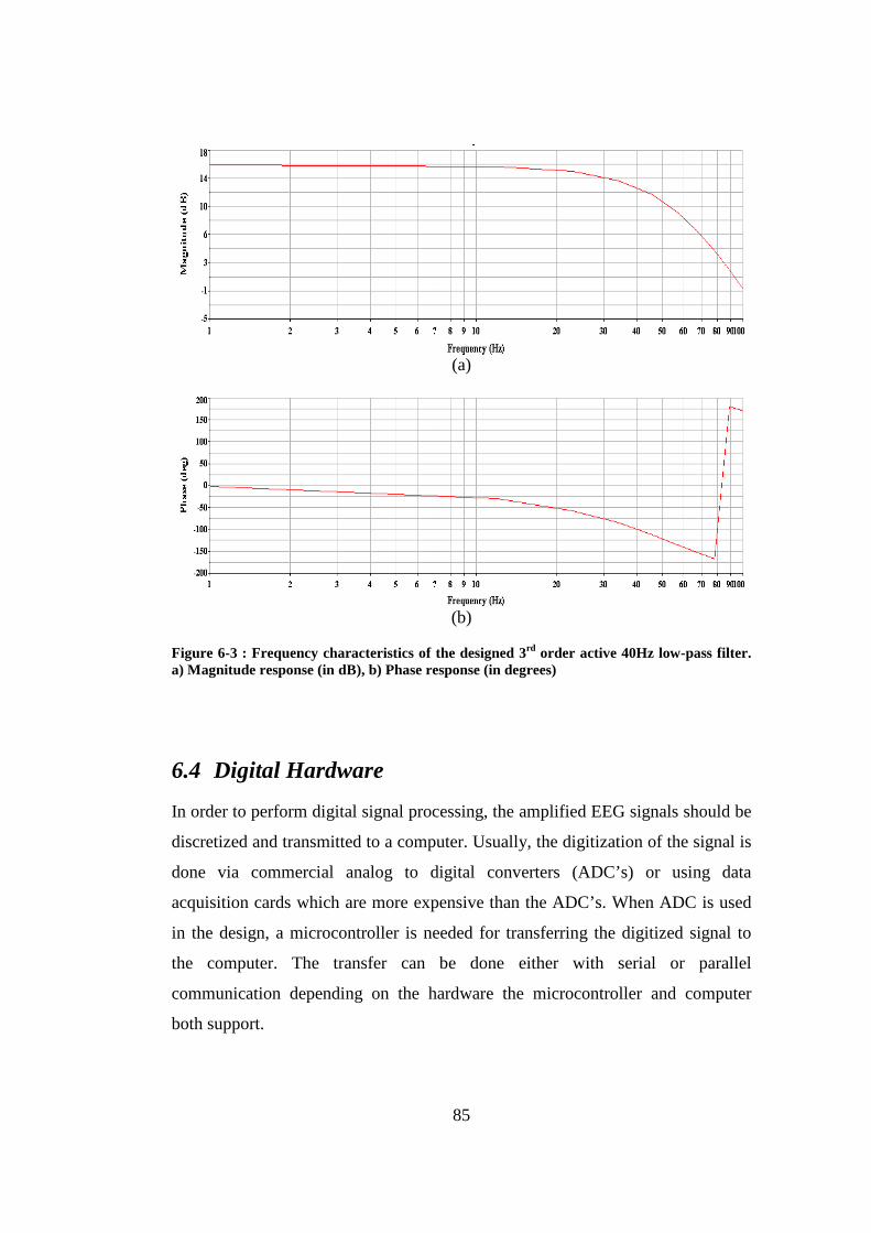
85
(a)
(b)
Figure 6-3 : Frequency characteristics of the designed 3rd order active 40Hz low-pass filter. a) Magnitude response (in dB), b) Phase response (in degrees)
6.4 Digital Hardware
In order to perform digital signal processing, the amplified EEG signals should be
discretized and transmitted to a computer. Usually, the digitization of the signal is
done via commercial analog to digital converters (ADC’s) or using data
acquisition cards which are more expensive than the ADC’s. When ADC is used
in the design, a microcontroller is needed for transferring the digitized signal to
the computer. The transfer can be done either with serial or parallel
communication depending on the hardware the microcontroller and computer
both support.

86
For today’s computers, Universal Serial Bus (USB) is the most common and
maybe the only communication platform due to its speed in transfer. And with the
development in technology, low cost microcontrollers with USB hardware are
available in the market which makes it easy to implement a USB communication
with the computer.
As stated in the introduction section in this chapter, it is aimed to design the EEG
hardware as minimum number of components as possible. Therefore, the digital
hardware is composed of PIC18F4553, a compact microcontroller with a high
ADC resolution and Full Speed (FS) USB hardware [79]. The hardware
schematics of the digital circuitry can be found in Appendix B.
6.5 Isolation
Isolation in medical systems is necessary for two reasons. The most important one
is that the electrical equipment can harm the subject when the isolation is poor.
Possible leakage currents can flow through subject’s body which can lead to
permanent disorders or even to deaths. In order to protect the subject from these
problems, subject has to be electrically isolated from the environment properly.
This can be performed by using isolated supplies like batteries or isolation
transformers for the analog amplifier which can decrease the risk of electrical
shock [83]. Moreover, the amplifier circuitry should be isolated from digital the
circuitry and the recording system due to possible reverse currents coming from
the computer side which can also harm the subject. In this design, standard
batteries are used in the analog circuitry for providing the supply isolation.
Isolation is also important for removing the effects of the noise caused by power
network, electrical equipments and high speed electronic devices like computers.
So, the analog and digital circuits should be electrically separated from those
devices by employing proper signal isolation in the system. Moreover, the ADC’s
used in these systems are usually affected from the signal oscillations in the

87
analog circuitry. This is mainly caused by the ground nodes the analog and digital
circuits are referenced and when they are implemented as the same node, the
ADC’s usually can not convert the signals accurately. Therefore, the analog and
digital grounds should also be isolated.
The signal isolation can be done with galvanic isolators, analog and digital
optocouplers, transformers or the isolation amplifiers in the circuit. In this design,
the amplified EEG signals are isolated from the digital circuitry with analog
optocouplers [80]. The reason for using optocouplers is that they occupy less
space in the circuit and cost less as compared with other isolator types. Moreover,
as the microcontroller used in this design has built-in USB device hardware, the
isolation can not be done digitally. Therefore, the analog optocoupling is
preferred and this provides an advantage of ground isolation between the analog
and digital circuits which results in better digitization of the signal at the ADC
stage.
6.6 EEG Cap Design
In commercial EEG systems, the electrodes are placed on an elastic head cap
according to the 10-20 electrode placement system [41], [43]. These caps are
suitable only for passive ring electrodes in which the electrodes are covered with
a conductive gel. Figure 6-5 shows a commercial EEG cap produced by
Neuroscan.
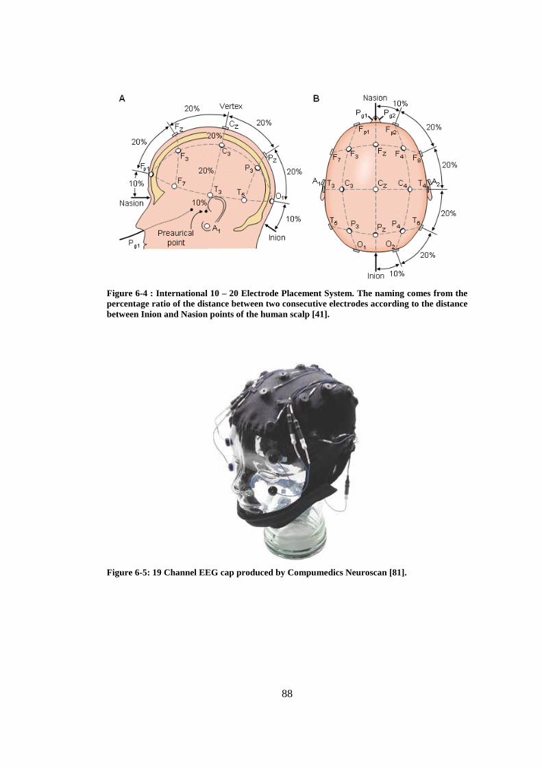
88
Figure 6-4 : International 10 – 20 Electrode Placement System. The naming comes from the percentage ratio of the distance between two consecutive electrodes according to the distance between Inion and Nasion points of the human scalp [41].
Figure 6-5: 19 Channel EEG cap produced by Compumedics Neuroscan [81].

89
However, when active electrodes are to be used in the system, the electrodes may
not be easily attached to the scalp due to their size and weight of the material in
the electrodes. For this reason, a cap design is performed for active electrodes in
which the placement of the electrodes is easy and the effect of common mode
noise is theoretically reduced (Figure 6-6).
Figure 6-6 : The effect of the designed EEG cap on reducing the common mode voltage induced on the body. The common mode voltage with respect to the amplifier ground is decreased as the distance between the amplifier ground and the electrode leads is small. Furthermore, the leakage currents are more likely to flow through the cap instead of the body with this configuration.
The designed EEG cap in Figure 6-7 is composed of three layers. The outer layer
is a Teflon material for holding and fixing the active electrodes on the scalp. In
the middle layer, there is a thin aluminum film which is used for a conductive
path to the analog ground. This film acts as a protective layer for the displacement
currents which can generate a common mode voltage in the preamplifier stage.
The inner layer is a soft tissue made up of Styrofoam which provides a soft
contact between the cap and the subject. 10 active electrodes are located on the
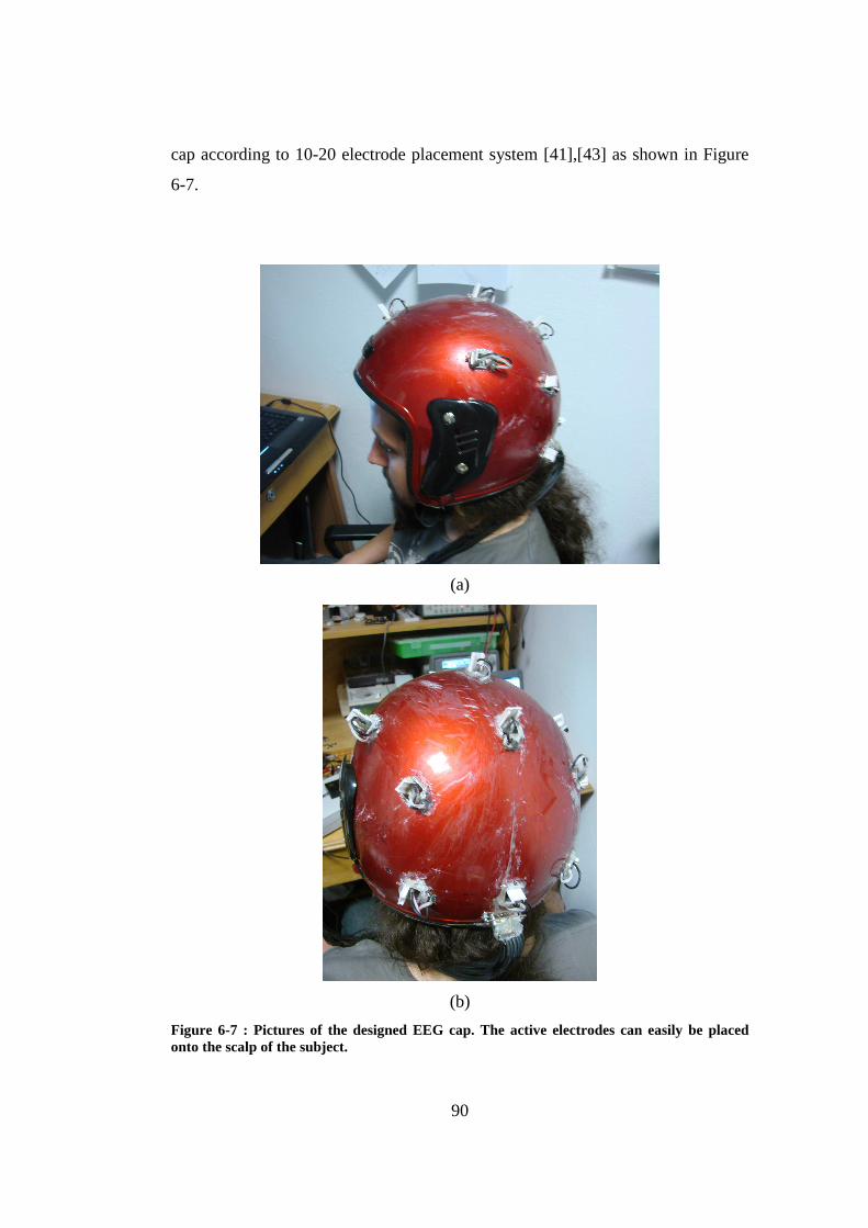
90
cap according to 10-20 electrode placement system [41],[43] as shown in Figure
6-7.
(a)
(b)
Figure 6-7 : Pictures of the designed EEG cap. The active electrodes can easily be placed onto the scalp of the subject.
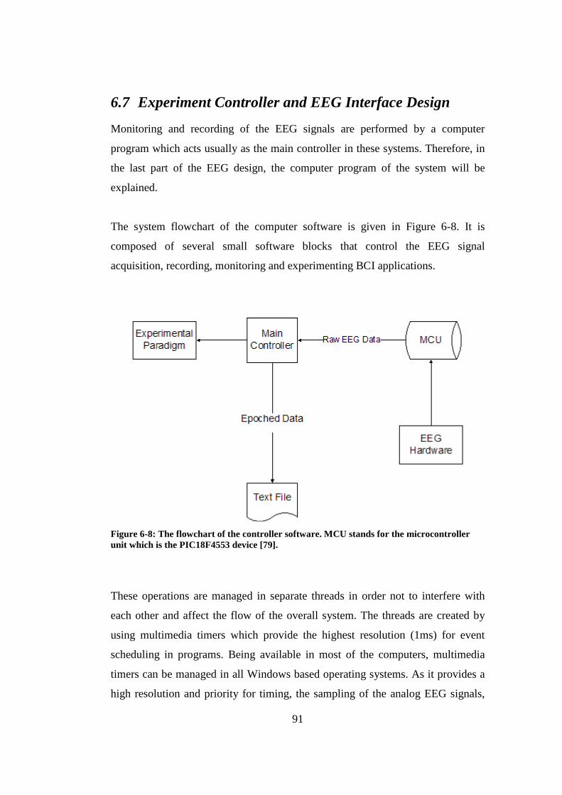
91
6.7 Experiment Controller and EEG Interface Design
Monitoring and recording of the EEG signals are performed by a computer
program which acts usually as the main controller in these systems. Therefore, in
the last part of the EEG design, the computer program of the system will be
explained.
The system flowchart of the computer software is given in Figure 6-8. It is
composed of several small software blocks that control the EEG signal
acquisition, recording, monitoring and experimenting BCI applications.
Figure 6-8: The flowchart of the controller software. MCU stands for the microcontroller unit which is the PIC18F4553 device [79].
These operations are managed in separate threads in order not to interfere with
each other and affect the flow of the overall system. The threads are created by
using multimedia timers which provide the highest resolution (1ms) for event
scheduling in programs. Being available in most of the computers, multimedia
timers can be managed in all Windows based operating systems. As it provides a
high resolution and priority for timing, the sampling of the analog EEG signals,

92
monitoring and recording of the data and the intensification timing in spelling
paradigm are all done with the multimedia timer instances.
The program is prepared in Visual Studio .NET 2005 which provides a useful
framework for computer applications based on object oriented programming
(OOP). It is controlled with a friendly graphical user interface allowing the EEG
operator to manage the EEG sessions easily.
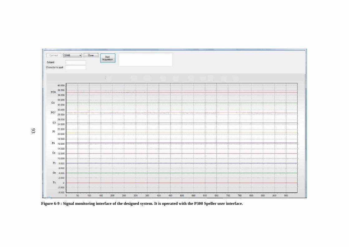
93
Figure 6-9 : Signal monitoring interface of the designed system. It is operated with the P300 Speller user interface.
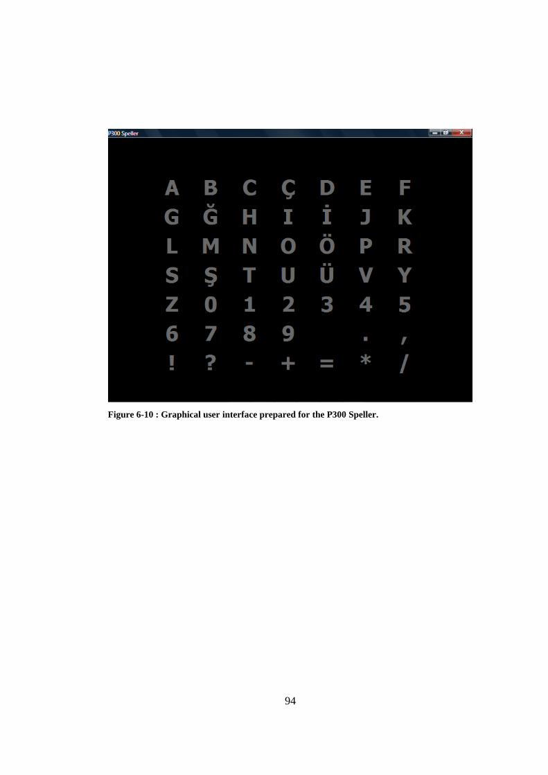
94
Figure 6-10 : Graphical user interface prepared for the P300 Speller.

95
CHAPTER 7
RESULTS
As stated in the introduction chapter, the Spelling Application is investigated in
several aspects which can mainly be summarized as the application type of
classification methods [77] (the analysis of classification performance by
separating the observations of row and column intensifications), the comparison
of Wiener filtering with standard filtering techniques and the effect of probability
estimation method by application of Maximum Likelihood Estimation in the
prediction mechanism of the target character. These aspects will be addressed in
this result chapter by performing the analysis case by case on several Spelling
Paradigm datasets.
In this study, the methodologies are tested on one of the BCI competition datasets
(the P300 Speller dataset of BCI Contest II [18]). An experimental dataset is
obtained for the spelling application at Dokuz Eylül University, in a shielded EEG
laboratory environment. Furthermore, a successful experimentation is performed
with the designed hardware at the Brain Research Laboratory of Electrical and
Electronics Department of Middle East Technical University. The results of the
presented methods will be provided after giving a brief explanation of each
dataset.
96
7.1 Results on the BCI Competition II: Dataset IIb
The P300 Speller datasets for BCI Competition II and III are provided by
Wadsworth BCI [14], in which the measurements are obtained with the BCI2000
system [15]. The datasets are publicly available at [18] and [20]. Here in this
thesis, only the results for the dataset of BCI Competition II [18] are presented
since the implemented methodologies could not be properly integrated to the
dataset of BCI Competition III due to the size of the provided dataset in this
contest and memory requirements of the employed methodologies.
In these experiments, the spelling matrix consists of 36 characters which are
distributed on 6 rows and 6 columns of the matrix (Figure 3-1). The
intensification procedure for each spelled character is performed by flashing a
row or column for 100ms and after that showing a blank screen (no intensified
rows and columns) for 75ms. Therefore, a single intensification lasts for 175ms
(5.7Hz) and as there are 6 row and 6 column intensifications, one trial of
intensification is completed after 2.1 seconds (175ms x 12 intensifications). After
each trial, a blank screen is presented for 2.5 seconds to inform the subject that
the trial is completed and the next trial is coming up. The intensification
procedure is repeated for 15 trials so that the whole procedure takes nearly 69
seconds to complete the spelling session of a single character ((2.1s of trial
duration+ 2.5s blank screen time) x 15 trials).
In both datasets, the EEG signals are digitized at a sampling rate of 240Hz and in
the dataset of BCI contest III only, the signals are band-pass filtered by hardware
with cut-off frequencies 0.1Hz and 60Hz. The information provided in these
datasets consists of the raw EEG data measured from 64 channels (Figure 7-1),
the codes of the intensification (Figure 7-2) and the target characters that are
spelled during those sessions.
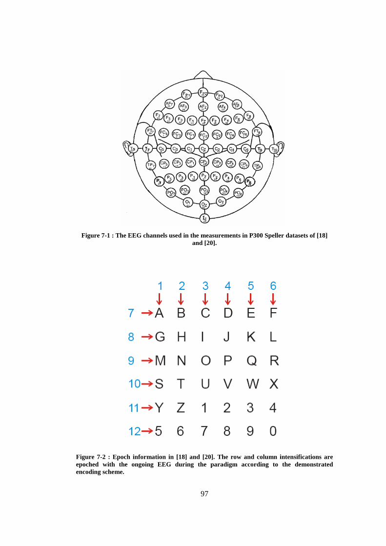
97
Figure 7-1 : The EEG channels used in the measurements in P300 Speller datasets of [18]
and [20].
Figure 7-2 : Epoch information in [18] and [20]. The row and column intensifications are epoched with the ongoing EEG during the paradigm according to the demonstrated encoding scheme.

98
The P300 Speller dataset of BCI Contest II [18] includes three spelling sessions
from one subject; two for training and one for testing the algorithms prepared for
this problem. Each session is composed of several runs in which the 3-5 letter
words are spelled4. The contents of these sessions are provided in Table 7-1 and
Table 7-2.
Table 7-1: Contents of the Training Sessions in Spelling Paradigm Dataset of BCI Contest II
Session 1 Session 2
Runs 1 2 3 4 5 1 2 3 4 5 6
Words CAT DOG FISH WATER BOWL HAT HAT GLOVE SHOES FISH RAT
Table 7-2: Contents of the Test Session in Spelling Paradigm Dataset of BCI Contest II
Session 3
Runs 1 2 3 4 5 6 7 8
Words FOOD MOOT HAM PIE CAKE TUNA ZYGOT 4567
As stated in chapter 3, the basis of this study relies on the success of the algorithm
proposed by Kaper et al [4]. In their work, they have employed Support Vector
Machines (SVM) [77] with a feature set configuration consisting of 10 EEG
channels (Figure 7-3 (a)). Moreover, commercial P300 Speller systems employ
even less number of electrode configuration in their methods [42] (Figure 7-3
(b)). Therefore, in this thesis, after the presentation of each stimulus, the EEG
time segments of 600ms duration from the channels in Figure 7-3 (a) are
extracted. As in [4], a long feature vector consisting of 1440 elements (600ms x
240Hz x 10 channels / 1000) is constructed to compare the methodologies
presented. Since it is only possible to perform offline analysis on the dataset, the
4 The data of the 6th run of Session 2 is somehow corrupted; it contains some bugs related to the recording process. Therefore, it is excluded in forming the classification model and hence in providing the results here.
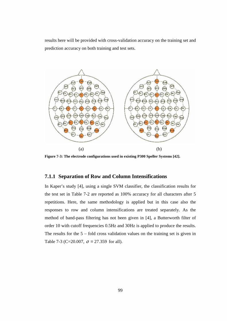
99
results here will be provided with cross-validation accuracy on the training set and
prediction accuracy on both training and test sets.
(a) (b)
Figure 7-3: The electrode configurations used in existing P300 Speller Systems [42].
7.1.1 Separation of Row and Column Intensifications
In Kaper’s study [4], using a single SVM classifier, the classification results for
the test set in Table 7-2 are reported as 100% accuracy for all characters after 5
repetitions. Here, the same methodology is applied but in this case also the
responses to row and column intensifications are treated separately. As the
method of band-pass filtering has not been given in [4], a Butterworth filter of
order 10 with cutoff frequencies 0.5Hz and 30Hz is applied to produce the results.
The results for the 5 – fold cross validation values on the training set is given in
Table 7-3 (C=20.007, 359.27=σ for all).
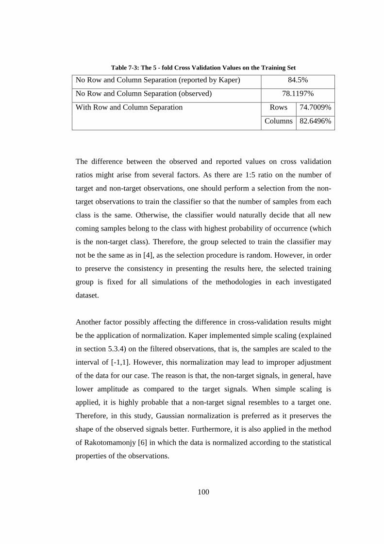
100
Table 7-3: The 5 - fold Cross Validation Values on the Training Set
No Row and Column Separation (reported by Kaper) 84.5%
No Row and Column Separation (observed) 78.1197%
Rows 74.7009% With Row and Column Separation
Columns 82.6496%
The difference between the observed and reported values on cross validation
ratios might arise from several factors. As there are 1:5 ratio on the number of
target and non-target observations, one should perform a selection from the non-
target observations to train the classifier so that the number of samples from each
class is the same. Otherwise, the classifier would naturally decide that all new
coming samples belong to the class with highest probability of occurrence (which
is the non-target class). Therefore, the group selected to train the classifier may
not be the same as in [4], as the selection procedure is random. However, in order
to preserve the consistency in presenting the results here, the selected training
group is fixed for all simulations of the methodologies in each investigated
dataset.
Another factor possibly affecting the difference in cross-validation results might
be the application of normalization. Kaper implemented simple scaling (explained
in section 5.3.4) on the filtered observations, that is, the samples are scaled to the
interval of [-1,1]. However, this normalization may lead to improper adjustment
of the data for our case. The reason is that, the non-target signals, in general, have
lower amplitude as compared to the target signals. When simple scaling is
applied, it is highly probable that a non-target signal resembles to a target one.
Therefore, in this study, Gaussian normalization is preferred as it preserves the
shape of the observed signals better. Furthermore, it is also applied in the method
of Rakotomamonjy [6] in which the data is normalized according to the statistical
properties of the observations.

101
As stated at the beginning of this section, the filter type has not been explained
clearly in [4]. The difference in the cross-validation values might also be caused
by this reasoning. Rakotomamonjy [6] applied an 8th order band-pass Chebyshev
Type 1 filter with cutoff frequencies 0.1Hz and 10Hz in their study for BCI
contest III. Both of these filter types are compared with the proposed Wiener
filtering in the following sections.
The 5-fold cross-validation values in Table 7-3 indicate that the rows and column
observation groups may not always be classified with the same accuracy. The
reason for this might be that the subject may exhibit different responses to row
and column intensifications. As the subject’s perception to row and column
flashings may differ, they should be treated and trained in separate classifiers to
increase the level of commonness and homogeneity in the training model.
Therefore, the 5-fold cross-validation is performed on row and column groups
independently and optimum parameters (the regularization parameter C in SVM
and the variance parameter σ in Gaussian RBF) providing the maximum cross
validation ratio are found (76.9231% for rows and 84.2735% for columns) for
each of them as 100=rC , 120=rσ and 40=cC , 60=cσ (see Table 7-4 below
for the comparison).
7.1.2 The Effect of Wiener Filtering
As discussed in chapter 3, the optimum frequency bands for P300 speller are
determined by estimating a Wiener filter for all EEG channels of interest. The
Wiener filters are produced by estimating a 10th order linear phase FIR
implementation for the frequencies found by the analysis of the spectral powers.
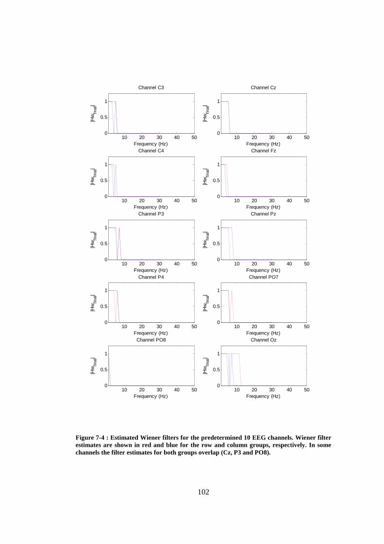
102
10 20 30 40 500
0.5
1
Frequency (Hz)
|Hw
final
|Channel C3
10 20 30 40 500
0.5
1
Frequency (Hz)
|Hw
final
|
Channel Cz
10 20 30 40 500
0.5
1
Frequency (Hz)
|Hw
final
|
Channel C4
10 20 30 40 500
0.5
1
Frequency (Hz)|H
wfin
al|
Channel Fz
10 20 30 40 500
0.5
1
Frequency (Hz)
|Hw
final
|
Channel P3
10 20 30 40 500
0.5
1
Frequency (Hz)
|Hw
final
|
Channel Pz
10 20 30 40 500
0.5
1
Frequency (Hz)
|Hw
final
|
Channel P4
10 20 30 40 500
0.5
1
Frequency (Hz)
|Hw
final
|
Channel PO7
10 20 30 40 500
0.5
1
Frequency (Hz)
|Hw
final
|
Channel PO8
10 20 30 40 500
0.5
1
Frequency (Hz)
|Hw
final
|
Channel Oz
Figure 7-4 : Estimated Wiener filters for the predetermined 10 EEG channels. Wiener filter estimates are shown in red and blue for the row and column groups, respectively. In some channels the filter estimates for both groups overlap (Cz, P3 and PO8).
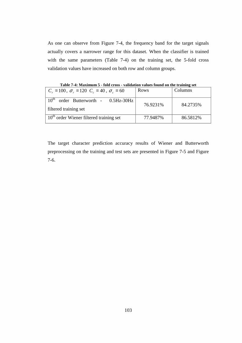
103
As one can observe from Figure 7-4, the frequency band for the target signals
actually covers a narrower range for this dataset. When the classifier is trained
with the same parameters (Table 7-4) on the training set, the 5-fold cross
validation values have increased on both row and column groups.
Table 7-4: Maximum 5 - fold cross - validation values found on the training set
100=rC , 120=rσ 40=cC , 60=cσ Rows Columns
10th order Butterworth - 0.5Hz-30Hz
filtered training set 76.9231% 84.2735%
10th order Wiener filtered training set 77.9487% 86.5812%
The target character prediction accuracy results of Wiener and Butterworth
preprocessing on the training and test sets are presented in Figure 7-5 and Figure
7-6.
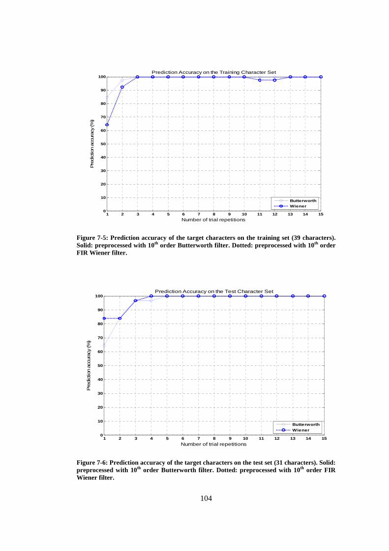
104
1 2 3 4 5 6 7 8 9 10 11 12 13 14 150
10
20
30
40
50
60
70
80
90
100
Number of trial repetitions
Pre
dict
ion
accu
racy
(%)
Prediction Accuracy on the Training Character Set
ButterworthWiener
Figure 7-5: Prediction accuracy of the target characters on the training set (39 characters). Solid: preprocessed with 10th order Butterworth filter. Dotted: preprocessed with 10th order FIR Wiener filter.
1 2 3 4 5 6 7 8 9 10 11 12 13 14 150
10
20
30
40
50
60
70
80
90
100
Number of trial repetitions
Pre
dict
ion
accu
racy
(%)
Prediction Accuracy on the Test Character Set
ButterworthWiener
Figure 7-6: Prediction accuracy of the target characters on the test set (31 characters). Solid: preprocessed with 10th order Butterworth filter. Dotted: preprocessed with 10th order FIR Wiener filter.
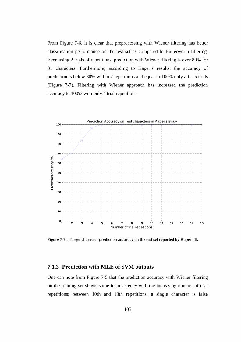
105
From Figure 7-6, it is clear that preprocessing with Wiener filtering has better
classification performance on the test set as compared to Butterworth filtering.
Even using 2 trials of repetitions, prediction with Wiener filtering is over 80% for
31 characters. Furthermore, according to Kaper’s results, the accuracy of
prediction is below 80% within 2 repetitions and equal to 100% only after 5 trials
(Figure 7-7). Filtering with Wiener approach has increased the prediction
accuracy to 100% with only 4 trial repetitions.
1 2 3 4 5 6 7 8 9 10 11 12 13 14 150
10
20
30
40
50
60
70
80
90
100
Number of trial repetitions
Pre
dict
ion
accu
racy
(%)
Prediction Accuracy on Test characters in Kaper's study
Figure 7-7 : Target character prediction accuracy on the test set reported by Kaper [4].
7.1.3 Prediction with MLE of SVM outputs
One can note from Figure 7-5 that the prediction accuracy with Wiener filtering
on the training set shows some inconsistency with the increasing number of trial
repetitions; between 10th and 13th repetitions, a single character is false
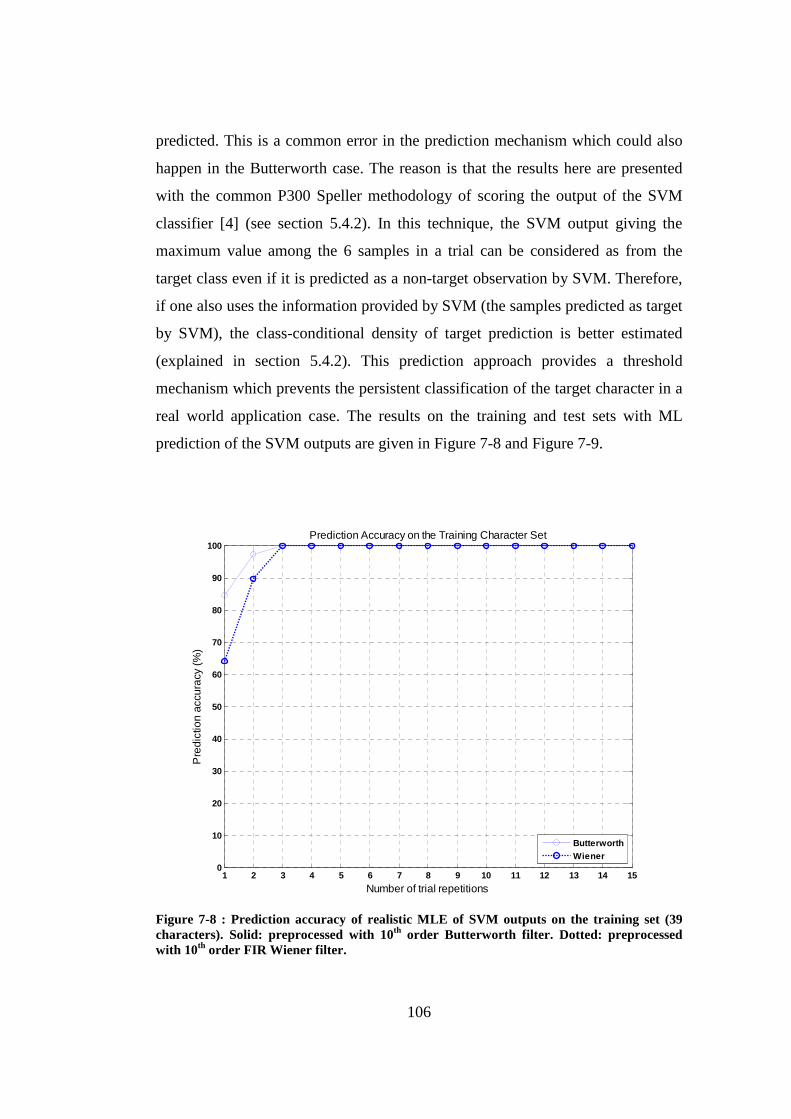
106
predicted. This is a common error in the prediction mechanism which could also
happen in the Butterworth case. The reason is that the results here are presented
with the common P300 Speller methodology of scoring the output of the SVM
classifier [4] (see section 5.4.2). In this technique, the SVM output giving the
maximum value among the 6 samples in a trial can be considered as from the
target class even if it is predicted as a non-target observation by SVM. Therefore,
if one also uses the information provided by SVM (the samples predicted as target
by SVM), the class-conditional density of target prediction is better estimated
(explained in section 5.4.2). This prediction approach provides a threshold
mechanism which prevents the persistent classification of the target character in a
real world application case. The results on the training and test sets with ML
prediction of the SVM outputs are given in Figure 7-8 and Figure 7-9.
1 2 3 4 5 6 7 8 9 10 11 12 13 14 150
10
20
30
40
50
60
70
80
90
100
Number of trial repetitions
Pre
dict
ion
accu
racy
(%)
Prediction Accuracy on the Training Character Set
ButterworthWiener
Figure 7-8 : Prediction accuracy of realistic MLE of SVM outputs on the training set (39 characters). Solid: preprocessed with 10th order Butterworth filter. Dotted: preprocessed with 10th order FIR Wiener filter.
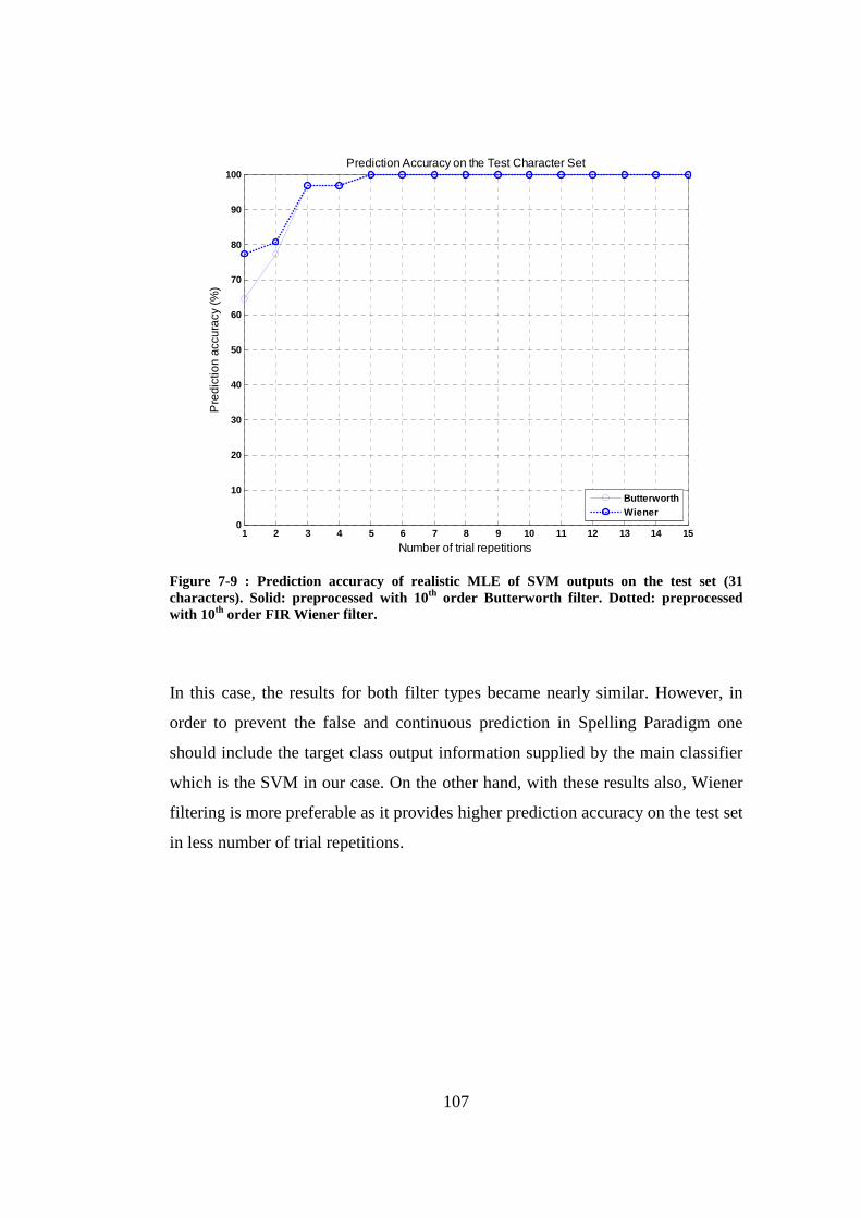
107
1 2 3 4 5 6 7 8 9 10 11 12 13 14 150
10
20
30
40
50
60
70
80
90
100
Number of trial repetitions
Pre
dict
ion
accu
racy
(%)
Prediction Accuracy on the Test Character Set
ButterworthWiener
Figure 7-9 : Prediction accuracy of realistic MLE of SVM outputs on the test set (31 characters). Solid: preprocessed with 10th order Butterworth filter. Dotted: preprocessed with 10th order FIR Wiener filter.
In this case, the results for both filter types became nearly similar. However, in
order to prevent the false and continuous prediction in Spelling Paradigm one
should include the target class output information supplied by the main classifier
which is the SVM in our case. On the other hand, with these results also, Wiener
filtering is more preferable as it provides higher prediction accuracy on the test set
in less number of trial repetitions.
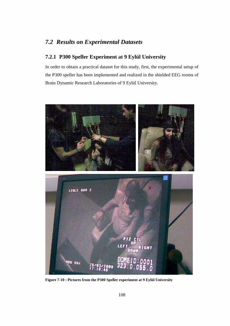
108
7.2 Results on Experimental Datasets
7.2.1 P300 Speller Experiment at 9 Eylül University
In order to obtain a practical dataset for this study, first, the experimental setup of
the P300 speller has been implemented and realized in the shielded EEG rooms of
Brain Dynamic Research Laboratories of 9 Eylül University.
Figure 7-10 : Pictures from the P300 Speller experiment at 9 Eylül University

109
The instrument used to measure the electrical activity of the brain is a 64 channel
EEG device of Neuroscan Systems which provides 1 kHz sampling of EEG
signals with active noise cancellation. The intensification algorithms for the
Spelling Paradigm experimental interface are integrated with the epoching
mechanism of the EEG system.
The experiment is performed on a healthy subject of age 24 (Figure 7-10) who did
not have any experience on evoked potential experiments. She is asked to stay
relaxed on a comfortable chair in front of a monitor on which the 6x6 spelling
matrix is presented. All operations are managed within the control room and in
case of a fatigue or any other problems related to the subject, she is monitored on
one of the screens in the control room.
In this experiment, the spelling application is performed for 35 characters in one
session which lasted about 2 hours. The procedure for spelling each character is
explained as follows:
• The subject is asked to focus on the predetermined characters on the 6x6
spelling matrix which are explained to the subject outside of the shielded
room via microphone. She is supposed to realize and silently count the
number of target row and column intensifications.
• As in the case of BCI Competition datasets, 15 trial repetitions are used in
spelling each character. For each trial, the intensifications are block
randomized for 6 rows and 6 columns.
• Since the subject had no experience on Spelling Paradigm, in order to
provide easy realization of the intensifications, the flashing duration is set
to 270ms (170ms on, 100ms off). The blank period between the trials is
kept at 2.5 seconds.

110
The characters spelled during the experiment are given in Table 7-5. The first 15
characters are used to construct the classification model and the remaining 20
characters are reserved for offline prediction.
Table 7-5: The characters spelled in the experimentation performed at 9 Eylül University Training Set
(15 characters)
Test Set
(20 characters)
Spelled words HECE BALKAR UGRAS BERNA URUN EKIM DEVRIM 7
As stated at the beginning of this section, the sampling rate of the recording EEG
system is 1 kHz which is nearly 4 times higher than that of the BCI contest
datasets. This results in a much longer feature vector, some of which, in fact, may
be redundant for classifying the target responses. Regarding the presented results
on the dataset of BCI Competitions II, the optimal frequency bands for detecting
the P300 responses lie mainly below 20Hz. Therefore, it is also possible to apply
downsampling to the EEG signals which is also employed in [6]. By this way, the
construction of the Wiener filter and SVM classification model will be much
faster as the computational power decreases with less number of feature samples.
Here, the results will be presented on downsampled data while investigating the
effects of Wiener and other filtering methodologies.
For the first case where the data is downsampled to 100Hz by taking the average
of blocks of consecutive 10 samples, the vector of interest is constructed with 600
ms long EEG segments from the predetermined 10 channels in Figure 7-3.
Therefore, the input space consists of 600 elements (600ms x 100Hz / 1000Hz x
10 channels). The Wiener filters estimated from the downsampled raw EEG data
for each channel are shown in Figure 7-11.
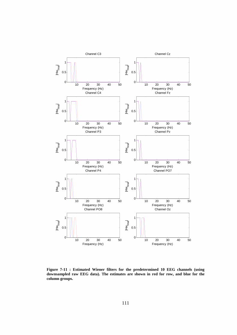
111
10 20 30 40 500
0.5
1
Frequency (Hz)
|Hw
final
|Channel C3
10 20 30 40 500
0.5
1
Frequency (Hz)
|Hw
final
|
Channel Cz
10 20 30 40 500
0.5
1
Frequency (Hz)
|Hw
final
|
Channel C4
10 20 30 40 500
0.5
1
Frequency (Hz)|H
wfin
al|
Channel Fz
10 20 30 40 500
0.5
1
Frequency (Hz)
|Hw
final
|
Channel P3
10 20 30 40 500
0.5
1
Frequency (Hz)
|Hw
final
|
Channel Pz
10 20 30 40 500
0.5
1
Frequency (Hz)
|Hw
final
|
Channel P4
10 20 30 40 500
0.5
1
Frequency (Hz)
|Hw
final
|
Channel PO7
10 20 30 40 500
0.5
1
Frequency (Hz)
|Hw
final
|
Channel PO8
10 20 30 40 500
0.5
1
Frequency (Hz)
|Hw
final
|
Channel Oz
Figure 7-11 : Estimated Wiener filters for the predetermined 10 EEG channels (using downsampled raw EEG data). The estimates are shown in red for row, and blue for the column groups.
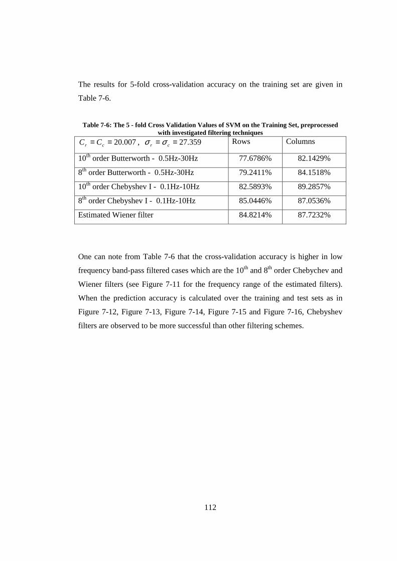
112
The results for 5-fold cross-validation accuracy on the training set are given in
Table 7-6.
Table 7-6: The 5 - fold Cross Validation Values of SVM on the Training Set, preprocessed with investigated filtering techniques
007.20== cr CC , 359.27== cr σσ Rows Columns
10th order Butterworth - 0.5Hz-30Hz 77.6786% 82.1429%
8th order Butterworth - 0.5Hz-30Hz 79.2411% 84.1518%
10th order Chebyshev I - 0.1Hz-10Hz 82.5893% 89.2857%
8th order Chebyshev I - 0.1Hz-10Hz 85.0446% 87.0536%
Estimated Wiener filter 84.8214% 87.7232%
One can note from Table 7-6 that the cross-validation accuracy is higher in low
frequency band-pass filtered cases which are the 10th and 8th order Chebychev and
Wiener filters (see Figure 7-11 for the frequency range of the estimated filters).
When the prediction accuracy is calculated over the training and test sets as in
Figure 7-12, Figure 7-13, Figure 7-14, Figure 7-15 and Figure 7-16, Chebyshev
filters are observed to be more successful than other filtering schemes.
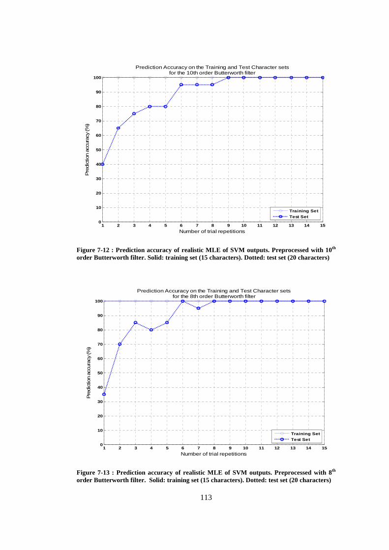
113
1 2 3 4 5 6 7 8 9 10 11 12 13 14 150
10
20
30
40
50
60
70
80
90
100
Number of trial repetitions
Pre
dict
ion
accu
racy
(%)
Prediction Accuracy on the Training and Test Character setsfor the 10th order Butterworth filter
Training SetTest Set
Figure 7-12 : Prediction accuracy of realistic MLE of SVM outputs. Preprocessed with 10th order Butterworth filter. Solid: training set (15 characters). Dotted: test set (20 characters)
1 2 3 4 5 6 7 8 9 10 11 12 13 14 150
10
20
30
40
50
60
70
80
90
100
Number of trial repetitions
Pre
dict
ion
accu
racy
(%)
Prediction Accuracy on the Training and Test Character setsfor the 8th order Butterworth filter
Training SetTest Set
Figure 7-13 : Prediction accuracy of realistic MLE of SVM outputs. Preprocessed with 8th order Butterworth filter. Solid: training set (15 characters). Dotted: test set (20 characters)
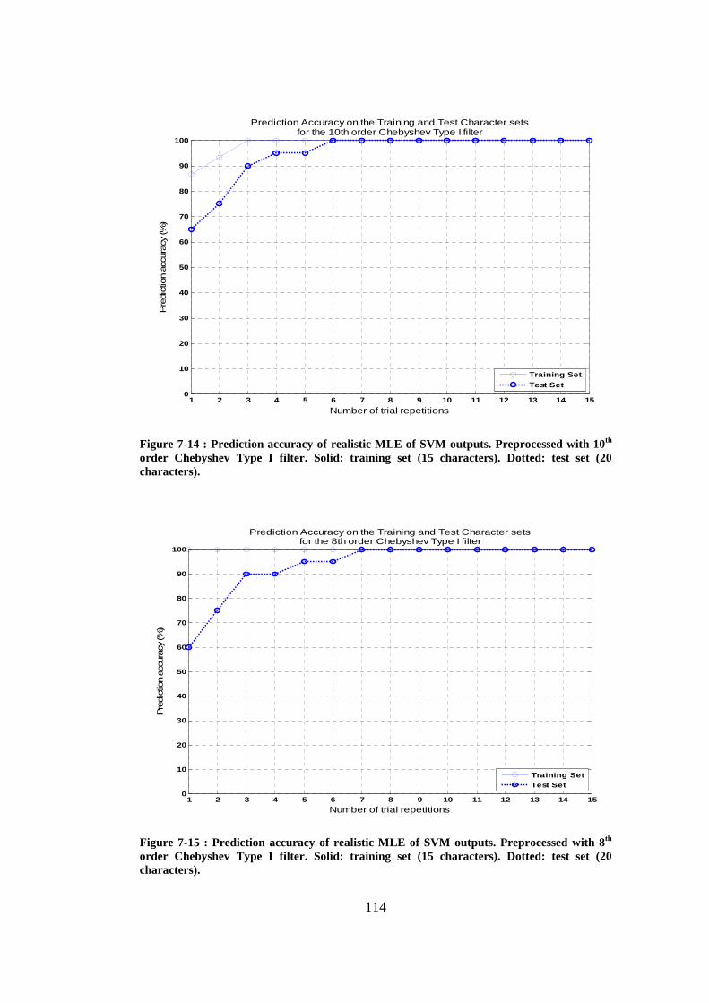
114
1 2 3 4 5 6 7 8 9 10 11 12 13 14 150
10
20
30
40
50
60
70
80
90
100
Number of trial repetitions
Pre
dict
ion
accu
racy
(%)
Prediction Accuracy on the Training and Test Character setsfor the 10th order Chebyshev Type I filter
Training SetTest Set
Figure 7-14 : Prediction accuracy of realistic MLE of SVM outputs. Preprocessed with 10th order Chebyshev Type I filter. Solid: training set (15 characters). Dotted: test set (20 characters).
1 2 3 4 5 6 7 8 9 10 11 12 13 14 150
10
20
30
40
50
60
70
80
90
100
Number of trial repetitions
Pre
dict
ion
accu
racy
(%)
Prediction Accuracy on the Training and Test Character setsfor the 8th order Chebyshev Type I filter
Training SetTest Set
Figure 7-15 : Prediction accuracy of realistic MLE of SVM outputs. Preprocessed with 8th order Chebyshev Type I filter. Solid: training set (15 characters). Dotted: test set (20 characters).
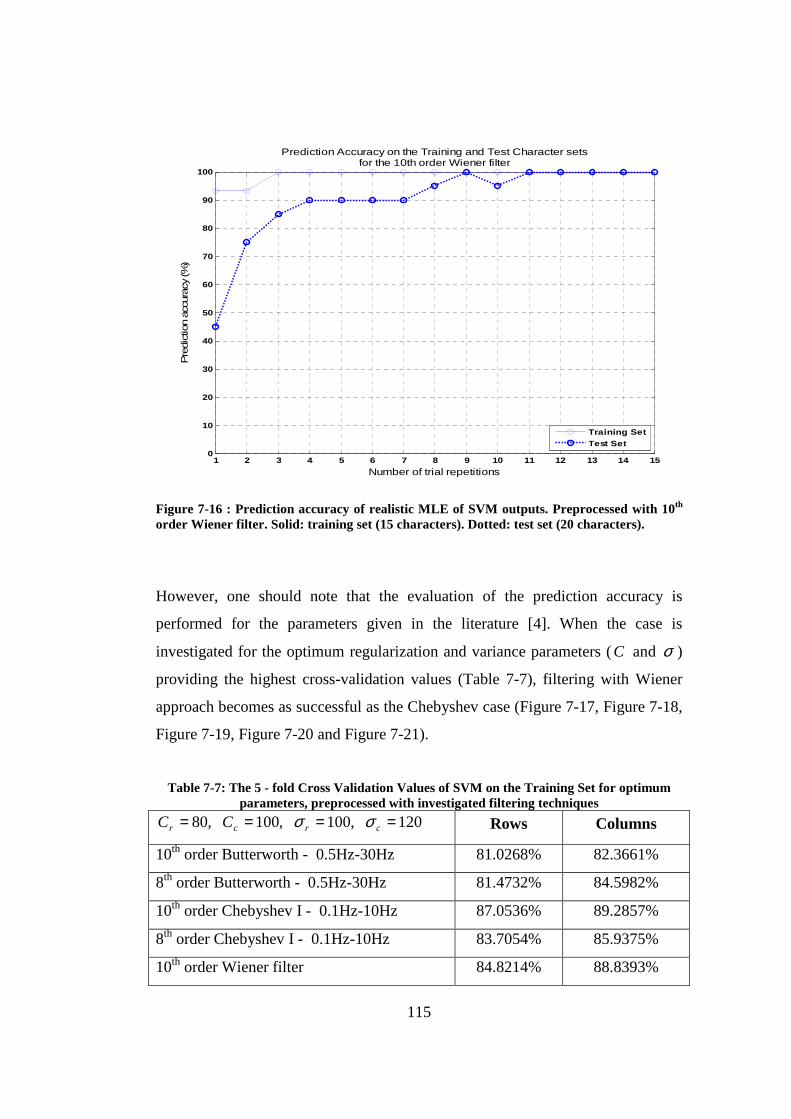
115
1 2 3 4 5 6 7 8 9 10 11 12 13 14 150
10
20
30
40
50
60
70
80
90
100
Number of trial repetitions
Pre
dict
ion
accu
racy
(%)
Prediction Accuracy on the Training and Test Character setsfor the 10th order Wiener filter
Training SetTest Set
Figure 7-16 : Prediction accuracy of realistic MLE of SVM outputs. Preprocessed with 10th order Wiener filter. Solid: training set (15 characters). Dotted: test set (20 characters).
However, one should note that the evaluation of the prediction accuracy is
performed for the parameters given in the literature [4]. When the case is
investigated for the optimum regularization and variance parameters (C and σ )
providing the highest cross-validation values (Table 7-7), filtering with Wiener
approach becomes as successful as the Chebyshev case (Figure 7-17, Figure 7-18,
Figure 7-19, Figure 7-20 and Figure 7-21).
Table 7-7: The 5 - fold Cross Validation Values of SVM on the Training Set for optimum parameters, preprocessed with investigated filtering techniques
120,100,100,80 ==== crcr CC σσ Rows Columns
10th order Butterworth - 0.5Hz-30Hz 81.0268% 82.3661%
8th order Butterworth - 0.5Hz-30Hz 81.4732% 84.5982%
10th order Chebyshev I - 0.1Hz-10Hz 87.0536% 89.2857%
8th order Chebyshev I - 0.1Hz-10Hz 83.7054% 85.9375%
10th order Wiener filter 84.8214% 88.8393%
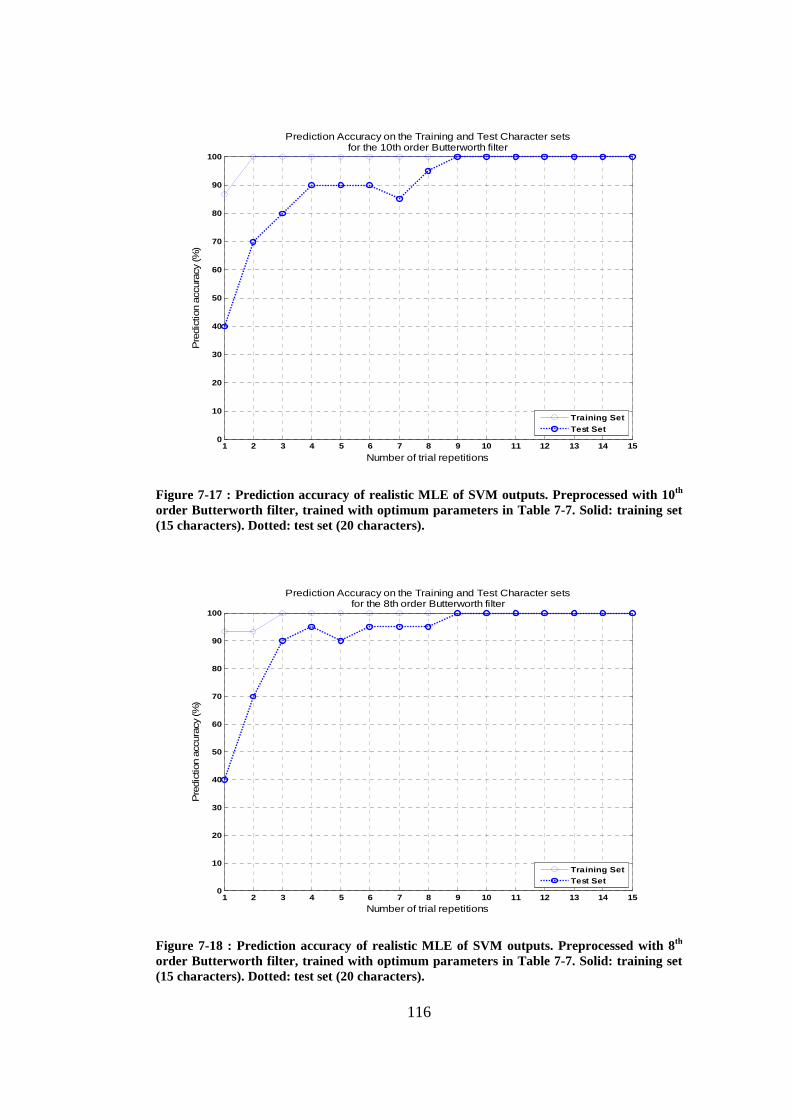
116
1 2 3 4 5 6 7 8 9 10 11 12 13 14 150
10
20
30
40
50
60
70
80
90
100
Number of trial repetitions
Pre
dict
ion
accu
racy
(%)
Prediction Accuracy on the Training and Test Character setsfor the 10th order Butterworth filter
Training SetTest Set
Figure 7-17 : Prediction accuracy of realistic MLE of SVM outputs. Preprocessed with 10th order Butterworth filter, trained with optimum para meters in Table 7-7. Solid: training set (15 characters). Dotted: test set (20 characters).
1 2 3 4 5 6 7 8 9 10 11 12 13 14 150
10
20
30
40
50
60
70
80
90
100
Number of trial repetitions
Pre
dict
ion
accu
racy
(%)
Prediction Accuracy on the Training and Test Character setsfor the 8th order Butterworth filter
Training SetTest Set
Figure 7-18 : Prediction accuracy of realistic MLE of SVM outputs. Preprocessed with 8th order Butterworth filter, trained with optimum para meters in Table 7-7. Solid: training set (15 characters). Dotted: test set (20 characters).
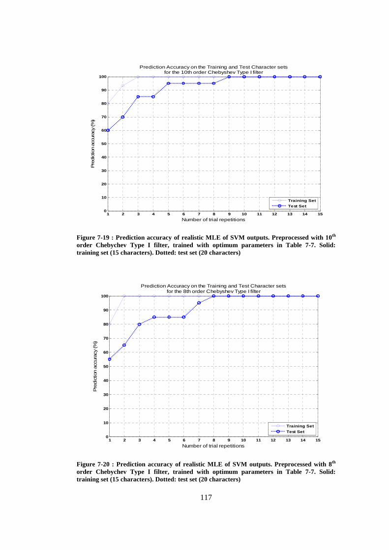
117
1 2 3 4 5 6 7 8 9 10 11 12 13 14 150
10
20
30
40
50
60
70
80
90
100
Number of trial repetitions
Pre
dict
ion
accu
racy
(%)
Prediction Accuracy on the Training and Test Character setsfor the 10th order Chebyshev Type I filter
Training SetTest Set
Figure 7-19 : Prediction accuracy of realistic MLE of SVM outputs. Preprocessed with 10th order Chebychev Type I filter, trained with optimum parameters in Table 7-7. Solid: training set (15 characters). Dotted: test set (20 characters)
1 2 3 4 5 6 7 8 9 10 11 12 13 14 150
10
20
30
40
50
60
70
80
90
100
Number of trial repetitions
Pre
dict
ion
accu
racy
(%)
Prediction Accuracy on the Training and Test Character setsfor the 8th order Chebyshev Type I filter
Training SetTest Set
Figure 7-20 : Prediction accuracy of realistic MLE of SVM outputs. Preprocessed with 8th order Chebychev Type I filter, trained with optimum parameters in Table 7-7. Solid: training set (15 characters). Dotted: test set (20 characters)
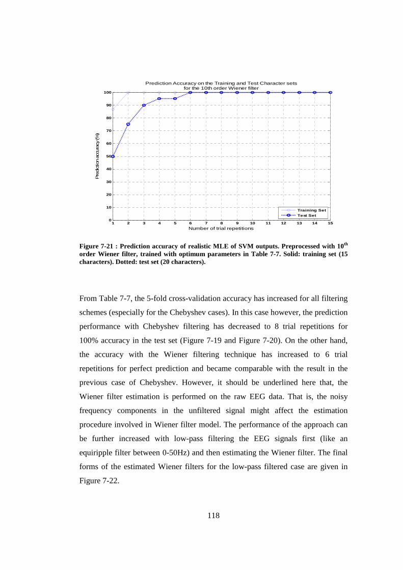
118
1 2 3 4 5 6 7 8 9 10 11 12 13 14 150
10
20
30
40
50
60
70
80
90
100
Number of trial repetitions
Pre
dict
ion
accu
racy
(%)
Prediction Accuracy on the Training and Test Character setsfor the 10th order Wiener filter
Training SetTest Set
Figure 7-21 : Prediction accuracy of realistic MLE of SVM outputs. Preprocessed with 10th order Wiener filter, trained with optimum parameter s in Table 7-7. Solid: training set (15 characters). Dotted: test set (20 characters).
From Table 7-7, the 5-fold cross-validation accuracy has increased for all filtering
schemes (especially for the Chebyshev cases). In this case however, the prediction
performance with Chebyshev filtering has decreased to 8 trial repetitions for
100% accuracy in the test set (Figure 7-19 and Figure 7-20). On the other hand,
the accuracy with the Wiener filtering technique has increased to 6 trial
repetitions for perfect prediction and became comparable with the result in the
previous case of Chebyshev. However, it should be underlined here that, the
Wiener filter estimation is performed on the raw EEG data. That is, the noisy
frequency components in the unfiltered signal might affect the estimation
procedure involved in Wiener filter model. The performance of the approach can
be further increased with low-pass filtering the EEG signals first (like an
equiripple filter between 0-50Hz) and then estimating the Wiener filter. The final
forms of the estimated Wiener filters for the low-pass filtered case are given in
Figure 7-22.

119
10 20 30 40 500
0.5
1
Frequency (Hz)
|Hw
final
|Channel C3
10 20 30 40 500
0.5
1
Frequency (Hz)
|Hw
final
|
Channel Cz
10 20 30 40 500
0.5
1
Frequency (Hz)
|Hw
final
|
Channel C4
10 20 30 40 500
0.5
1
Frequency (Hz)|H
wfin
al|
Channel Fz
10 20 30 40 500
0.5
1
Frequency (Hz)
|Hw
final
|
Channel P3
10 20 30 40 500
0.5
1
Frequency (Hz)
|Hw
final
|
Channel Pz
10 20 30 40 500
0.5
1
Frequency (Hz)
|Hw
final
|
Channel P4
10 20 30 40 500
0.5
1
Frequency (Hz)
|Hw
final
|
Channel PO7
10 20 30 40 500
0.5
1
Frequency (Hz)
|Hw
final
|
Channel PO8
10 20 30 40 500
0.5
1
Frequency (Hz)
|Hw
final
|
Channel Oz
Figure 7-22 : Estimated Wiener filters for the predetermined 10 EEG channels (estimated from the downsampled, 50Hz low-pass filtered EEG data). The estimates are shown in red for row, and blue for the column groups.
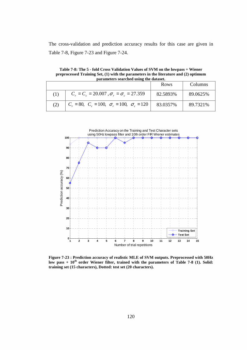
120
The cross-validation and prediction accuracy results for this case are given in
Table 7-8, Figure 7-23 and Figure 7-24.
Table 7-8: The 5 - fold Cross Validation Values of SVM on the lowpass + Wiener preprocessed Training Set, (1) with the parameters in the literature and (2) optimum
parameters searched using the dataset. Rows Columns
(1) 007.20== cr CC , 359.27== cr σσ 82.5893% 89.0625%
(2) 120,100,100,80 ==== crcr CC σσ 83.0357% 89.7321%
1 2 3 4 5 6 7 8 9 10 11 12 13 14 150
10
20
30
40
50
60
70
80
90
100
Number of trial repetitions
Pre
dict
ion
accu
racy
(%)
Prediction Accuracy on the Training and Test Character setsusing 50Hz lowpass filter and 10th order FIR Wiener estimates
Training SetTest Set
Figure 7-23 : Prediction accuracy of realistic MLE of SVM outputs. Preprocessed with 50Hz low pass + 10th order Wiener filter, trained with the parameters of Table 7-8 (1). Solid: training set (15 characters), Dotted: test set (20 characters).
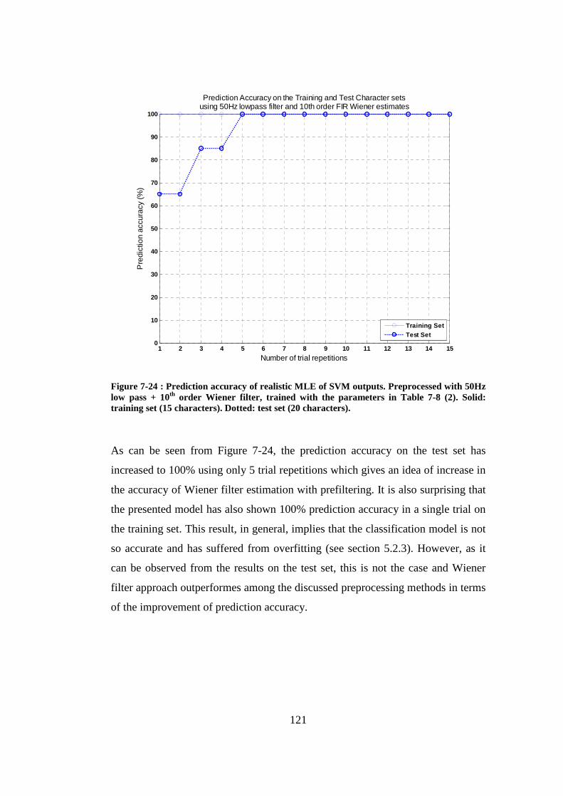
121
1 2 3 4 5 6 7 8 9 10 11 12 13 14 150
10
20
30
40
50
60
70
80
90
100
Number of trial repetitions
Pre
dict
ion
accu
racy
(%)
Prediction Accuracy on the Training and Test Character setsusing 50Hz lowpass filter and 10th order FIR Wiener estimates
Training SetTest Set
Figure 7-24 : Prediction accuracy of realistic MLE of SVM outputs. Preprocessed with 50Hz low pass + 10th order Wiener filter, trained with the parameters in Table 7-8 (2). Solid: training set (15 characters). Dotted: test set (20 characters).
As can be seen from Figure 7-24, the prediction accuracy on the test set has
increased to 100% using only 5 trial repetitions which gives an idea of increase in
the accuracy of Wiener filter estimation with prefiltering. It is also surprising that
the presented model has also shown 100% prediction accuracy in a single trial on
the training set. This result, in general, implies that the classification model is not
so accurate and has suffered from overfitting (see section 5.2.3). However, as it
can be observed from the results on the test set, this is not the case and Wiener
filter approach outperformes among the discussed preprocessing methods in terms
of the improvement of prediction accuracy.

122
7.2.2 Experimentation with the Designed Hardware
In the final section of this chapter, the results obtained from the Spelling
experiment with the designed EEG system are presented. The experiment is
conducted on a single subject with the conditions and procedure stated below:
• The measurement environment had no electrical shielding. Two
continuously running PC clusters of 8 computers each were working
nearby the recording room.
• The experiment was conducted in a dark environment.
• The subject was asked to sit relaxed on a standard chair without arms.
• A 7x7 spelling matrix composed of Turkish letters and other alphanumeric
characters were presented to the subject (Figure 7-26).
• The EEG signals were measured using the designed active electrodes
located on the predetermined positions on the scalp (Figure 7-3). The
ground and the active reference electrodes are positioned on FPz and right
ear respectively.
• For each spelled character, the recording of EEG signals was started after
a 10 seconds of preparation time. During this interval, the subject got
ready for the intensification sequences.
• The intensifications were randomized in blocks of 14 for 7 rows and 7
columns. The interstimulus interval was set to 250ms in which a row or
column was flashed on for 150ms and then flashed off for 100ms.
• A total of 15 trial repetitions were employed for all the characters in the
spelling session. The break time between the trials was adjusted to 1
second. Therefore, the spelling run for each character lasted about 77.5
seconds (10 seconds preparation time + (14 intensifications x 250 ms +
1000 ms break) x 15 repetitions).
• As the experiment employed 14 different intensifications and 15 trial
repetitions for each character, a spelling run consists of 210 observations
out of which there are 30 target and 180 non-target observations (2 targets
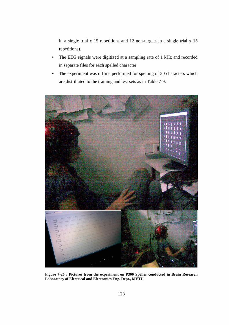
123
in a single trial x 15 repetitions and 12 non-targets in a single trial x 15
repetitions).
• The EEG signals were digitized at a sampling rate of 1 kHz and recorded
in separate files for each spelled character.
• The experiment was offline performed for spelling of 20 characters which
are distributed to the training and test sets as in Table 7-9.
Figure 7-25 : Pictures from the experiment on P300 Speller conducted in Brain Research Laboratory of Electrical and Electronics Eng. Dept., METU

124
Figure 7-26 : The spelling matrix and stimulus codes used in the experimentation performed with the designed hardware.
Table 7-9: The characters spelled in the experimentation conducted with the designed hardware
Training Set (9 characters) Test Set (11 characters)
Spelled words BERNA29BA BFKRTL7ÜHP3
7.2.2.1 Results on the EEG measurements
For visualization of the recorded target and non-target responses, the averaged
EEG signals from each class are shown in Figure 7-27 and Figure 7-28. From
these figures, it is clear that the developed EEG system accurately measured the
target P300 and non-target responses during the experiment.
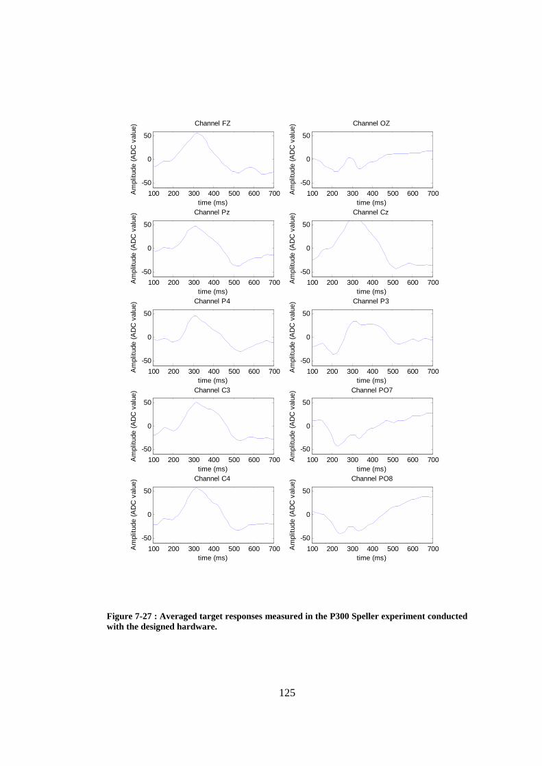
125
100 200 300 400 500 600 700
-50
0
50
time (ms)
Am
plitu
de (
AD
C v
alue
) Channel FZ
100 200 300 400 500 600 700
-50
0
50
time (ms)
Am
plitu
de (
AD
C v
alue
) Channel OZ
100 200 300 400 500 600 700
-50
0
50
time (ms)
Am
plitu
de (
AD
C v
alue
) Channel Pz
100 200 300 400 500 600 700
-50
0
50
time (ms)A
mpl
itude
(A
DC
val
ue) Channel Cz
100 200 300 400 500 600 700
-50
0
50
time (ms)
Am
plitu
de (
AD
C v
alue
) Channel P4
100 200 300 400 500 600 700
-50
0
50
time (ms)
Am
plitu
de (
AD
C v
alue
) Channel P3
100 200 300 400 500 600 700
-50
0
50
time (ms)
Am
plitu
de (
AD
C v
alue
) Channel C3
100 200 300 400 500 600 700
-50
0
50
time (ms)
Am
plitu
de (
AD
C v
alue
) Channel PO7
100 200 300 400 500 600 700
-50
0
50
time (ms)
Am
plitu
de (
AD
C v
alue
) Channel C4
100 200 300 400 500 600 700
-50
0
50
time (ms)
Am
plitu
de (
AD
C v
alue
) Channel PO8
Figure 7-27 : Averaged target responses measured in the P300 Speller experiment conducted with the designed hardware.
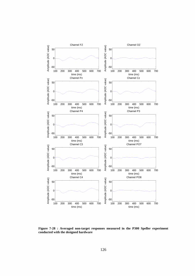
126
100 200 300 400 500 600 700
-50
0
50
time (ms)
Am
plitu
de (
AD
C v
alue
) Channel FZ
100 200 300 400 500 600 700
-50
0
50
time (ms)
Am
plitu
de (
AD
C v
alue
) Channel OZ
100 200 300 400 500 600 700
-50
0
50
time (ms)
Am
plitu
de (
AD
C v
alue
) Channel Pz
100 200 300 400 500 600 700
-50
0
50
time (ms)A
mpl
itude
(A
DC
val
ue) Channel Cz
100 200 300 400 500 600 700
-50
0
50
time (ms)
Am
plitu
de (
AD
C v
alue
) Channel P4
100 200 300 400 500 600 700
-50
0
50
time (ms)
Am
plitu
de (
AD
C v
alue
) Channel P3
100 200 300 400 500 600 700
-50
0
50
time (ms)
Am
plitu
de (
AD
C v
alue
) Channel C3
100 200 300 400 500 600 700
-50
0
50
time (ms)
Am
plitu
de (
AD
C v
alue
) Channel PO7
100 200 300 400 500 600 700
-50
0
50
time (ms)
Am
plitu
de (
AD
C v
alue
) Channel C4
100 200 300 400 500 600 700
-50
0
50
time (ms)
Am
plitu
de (
AD
C v
alue
) Channel PO8
Figure 7-28 : Averaged non-target responses measured in the P300 Speller experiment conducted with the designed hardware

127
7.2.2.2 Offline Analysis Procedure
The steps followed in preprocessing and classification of these datasets is
summarized below:
Preprocessing
Single trial extraction: EEG time segments of 600ms length, 100ms after the
presentation of visual stimuli are extracted.
Filtering: Although the EEG hardware employs active analog band-stop and low-
pass filters in its design, the extracted time segments are digitally filtered with an
equiripple low pass filter with a cutoff frequency of 50Hz.
Decimation: In order to reduce the dimensionality of the input space, the filtered
time segments are downsampled to 100Hz by taking the average of every 10
consecutive samples. Therefore, the number of time samples for each channel has
been reduced to 60.
Wiener filter estimation: The decimated observations are separated into row and
column groups and for each group the Wiener filter estimation is performed.
Construction of the feature vector: All Wiener filtered EEG segments are
concatenated by channel for each observation and a long feature vector is
constructed with 600 elements (60 samples x 10 channels).
Training
Grouping row and column observations: The preprocessed observations are
separated into row and column groups and for each group the data is divided into
target and non-target classes.
Selection of observations: From each trial, 1 target and 1 non-target observation is
selected to construct the SVM classifier for each group.

128
Search of parameters: For maximum cross-validation accuracy on the training
set, the regularization parameter C and the variance parameter σ are searched
for both groups between the interval [10, 200] with increments of 5. This is a time
consuming procedure and once the optimum values are found these parameters
are kept as constants for the SVM classifiers.
7.2.2.3 Results of the Proposed Methodologies
The estimated Wiener Filters are shown in Figure 7-29. One can note that the
optimum frequency bands for the row and column groups can show difference in
some of the EEG channels.
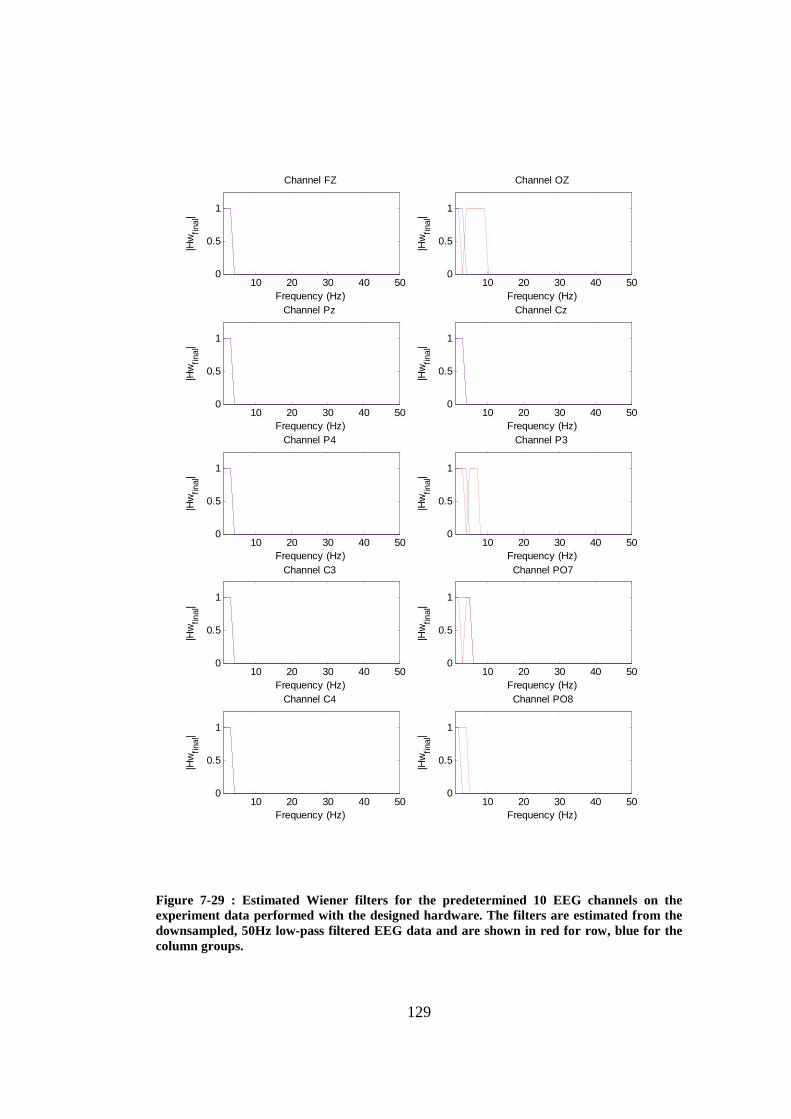
129
10 20 30 40 500
0.5
1
Frequency (Hz)
|Hw
final
|Channel FZ
10 20 30 40 500
0.5
1
Frequency (Hz)
|Hw
final
|
Channel OZ
10 20 30 40 500
0.5
1
Frequency (Hz)
|Hw
final
|
Channel Pz
10 20 30 40 500
0.5
1
Frequency (Hz)|H
wfin
al|
Channel Cz
10 20 30 40 500
0.5
1
Frequency (Hz)
|Hw
final
|
Channel P4
10 20 30 40 500
0.5
1
Frequency (Hz)
|Hw
final
|
Channel P3
10 20 30 40 500
0.5
1
Frequency (Hz)
|Hw
final
|
Channel C3
10 20 30 40 500
0.5
1
Frequency (Hz)
|Hw
final
|
Channel PO7
10 20 30 40 500
0.5
1
Frequency (Hz)
|Hw
final
|
Channel C4
10 20 30 40 500
0.5
1
Frequency (Hz)
|Hw
final
|
Channel PO8
Figure 7-29 : Estimated Wiener filters for the predetermined 10 EEG channels on the experiment data performed with the designed hardware. The filters are estimated from the downsampled, 50Hz low-pass filtered EEG data and are shown in red for row, blue for the column groups.
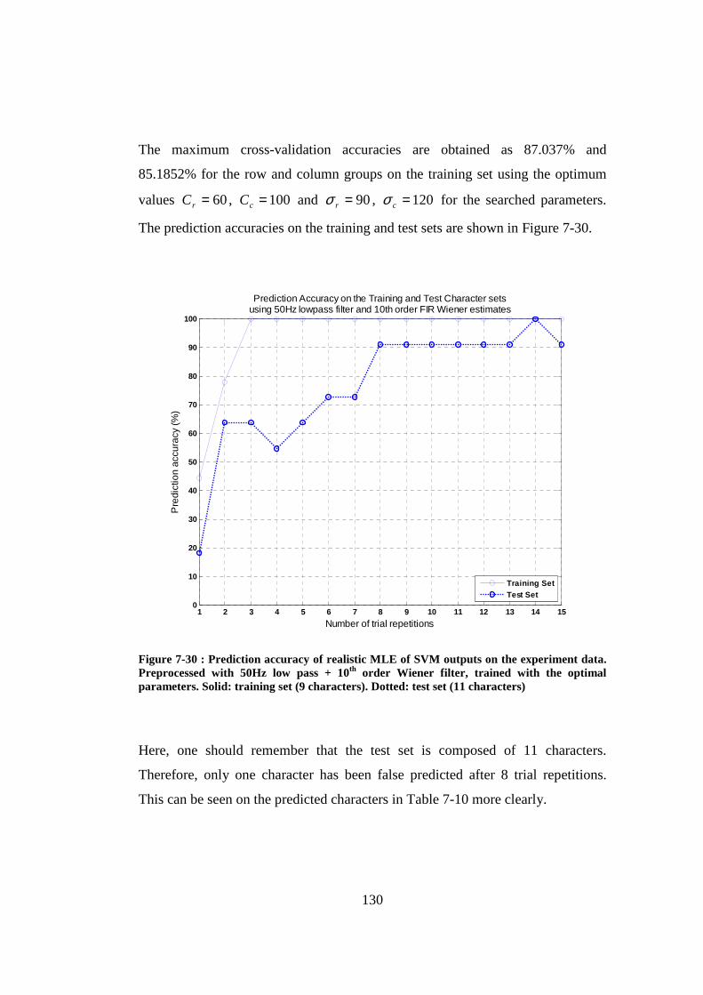
130
The maximum cross-validation accuracies are obtained as 87.037% and
85.1852% for the row and column groups on the training set using the optimum
values 60=rC , 100=cC and 90=rσ , 120=cσ for the searched parameters.
The prediction accuracies on the training and test sets are shown in Figure 7-30.
1 2 3 4 5 6 7 8 9 10 11 12 13 14 150
10
20
30
40
50
60
70
80
90
100
Number of trial repetitions
Pre
dict
ion
accu
racy
(%)
Prediction Accuracy on the Training and Test Character setsusing 50Hz lowpass filter and 10th order FIR Wiener estimates
Training SetTest Set
Figure 7-30 : Prediction accuracy of realistic MLE of SVM outputs on the experiment data. Preprocessed with 50Hz low pass + 10th order Wiener filter, trained with the optimal parameters. Solid: training set (9 characters). Dotted: test set (11 characters)
Here, one should remember that the test set is composed of 11 characters.
Therefore, only one character has been false predicted after 8 trial repetitions.
This can be seen on the predicted characters in Table 7-10 more clearly.

131
Table 7-10: Predicted characters in the test set with respect to the trial repetition number
Trials Predicted Characters
1 ĞKKR6G,T9ÖI
2 BFPMTL7Ü8PÇ
3 BFRRTG7Ü8PD
4 FFRRTG7Ü8PD
5 FEKRT!7ÜHPD
6 BEKRTG7ÜHPD
7 B,KRTG7ÜHPD
8 BFKRTL7ÜHPD
9 BFKRTL7ÜHPD
10 BFKRTL7ÜHPD
11 BFKRTL7ÜHPD
12 BFKRTL7ÜHPD
13 BFKRTL7ÜHPD
14 BFKRTL7ÜHP3
15 BFKRTL7ÜHPD
The only misclassified character in Table 7-10 after 8 trials (omitting the
exception in the 14th repetition) is the last one in which the subject informed that
she was not well concentrated on the character in the spelling session due to the
headache she suffered from. Omitting this case, the methodologies predicted the
characters with 100% accuracy using only 8 trials.
132
CHAPTER 8
CONCLUSION
In this thesis, the implementation of the P300 Speller system is performed by the
development of a P300 based BCI system. Several experiments are conducted
with the designed system in which the measurements are realized with the active
electrodes. Convincing performance is obtained in these experiments as the
system was able to measure the P300 patterns required for the spelling
application.
Wiener filtering, a statistical signal processing technique, is employed as a signal
enhancement method on the P300 speller for the first time in the literature. The
optimum frequency bands for P300 detection is investigated by estimating the
Wiener filters for the target and non-target observations. It is applied to several
P300 Speller datasets and observed to be more successful than the other filtering
techniques in terms of target character prediction accuracy. Furthermore, the rows
and columns of the spelling matrix are treated in separate groups in order to
investigate the difference in classification accuracies between these two
intensification types. In the P300 Speller dataset of BCI Competition II, the target
characters in the test set are predicted with 100% accuracy within 4 trials which is
higher than that of the prediction results of competition winners. On the other
hand, the prediction of the target characters with the designed system is
performed after 8 trials in order to obtain a perfect accuracy for all characters.
133
8.1 General Observations and Discussion
Several results are deducted from the observations on the investigated Spelling
Paradigm datasets. The first and maybe the most important observation is that the
brain responses to row and column intensifications are not classified with equal
accuracy. One can see from the cross-validation results that, (although treated in
the same way) the row groups usually have lower classification accuracy than the
column group for equal regularization and variance parameters (see section 7.1.1).
Even for the optimal values of the cross-validation results, the row group is
observed to be more misclassified than the column one. Although not presented
here, the single vector classification results were also higher for the column group
for each of the observed training and test sets. To give an example, in the
experimental study with the designed system, the misclassified character was
lying on the same column with the predicted character after 8 repetitions. The
column prediction was correct, but not the row. Therefore, it can be inferred that
the human perception to the row and column intensifications can be different for
each subject in terms of the brain’s responses which is an open research topic for
the neurophysiologists and psychologists interested in BCI. Furthermore, in order
to satisfy a successful classification scheme, these intensification groups should
be trained and classified separately on two classification modalities.
Another important deduction is that the optimum frequency band for P300
detection is in fact narrower than the normal EEG frequency range (0-45Hz). The
unnecessary frequency components outside this range can be eliminated for better
classification results. Whether the filtering technique is performed with Wiener
approach or not, filtering the out-of-range components considerably increases the
performance of the classification. Filtering with Wiener approach only provides
the frequency information that is optimal in detection of the measured signal.
Furthermore, one should note that the application of Wiener filtering on the P300
Speller problem is only meaningful with the assumptions described in chapter 4.
134
The stationarity of the signal patterns are of special importance in this
methodology. Unlike the common sense that the EEG measurements are non-
stationary signals [2], in this study, they are treated as stationary by employing a
WSS model of the P300 pattern and the noise signals. This modality is proven to
be valid for the P300 detection problem in Spelling Paradigm as the results show
that the filtering with the Wiener approach yielded the best classification
performance in SVM among the other preprocessing techniques (see sections
7.1.2 and 7.2.1). Furthermore, the presented approach is performed by the
estimation of the Wiener filters from the raw EEG data. It can be further
improved by estimating these after prefiltering the raw EEG signal first, with a
low-pass filtering method as described in section 7.2.1.
The performance of the classification depends on many parameters like the
selection of the training group, the type of normalization and the separation of the
row and column intensification groups. The cross-validation results, hence the
accuracy of the trained models is considerably affected by the samples selected to
train the classifiers. In order to perform a rational comparison between the
preprocessing and other methods, it is highly necessary to use the same group in
training the classifiers for all investigated filtering cases. Otherwise, the
performance of the classification method could vary (even for the same method)
in the second run of the algorithm.
In addition, the results presented in this thesis are obtained by performing a
Gaussian normalization on the datasets. The preprocessing methodologies in the
literature could have higher performance in here if they were investigated for all
normalization types discussed in section 5.3.4. However, the results for these
cases are believed to be variable on every P300 Speller dataset as the feature
patterns concerned here are more likely to be random signals. The shape and
amplitude of these signals might not be as well preserved as the Gaussian
normalization when compared to other normalization types. A deeper study is
needed to validate this assumption though.

135
Another important factor is that the classification results might not show the same
behaviour among the preprocessing techniques. That is, the parameters which are
optimal for one technique may not be as much optimal as the other one.
Therefore, they should be investigated for the cases in which they exhibit the
maximum cross validation accuracy on the training set. However, fortunately in
the presented results, all preprocessing techniques exhibited nearly the same
behavior in classification accuracies (except the Chebyshev case in section 7.2.1).
Finally, it should be underlined here that the performance of the overall system is
more dependent on the employed discriminative classification method. In most
cases, the target characters can be predicted by using a powerful classifier
exhibiting a 100% accuracy (may be at the 15th trial repetition) without any
preprocessing method. Therefore, the main success of this system is determined
by the SVM classifier [77]. Other methodologies can only serve slight
improvements in speed of the system as compared among each other.
8.2 Advantages of the Developed System and Methods
The proposed methodologies provide several advantages for the spelling
application in terms of practicality in the EEG measurements and preprocessing
mechanisms. The active electrodes employed in the system eliminate the need for
skin preparation stage applied in the passive counterpart. Using active electrodes
provides longer EEG measurements, thus improves the usability of a BCI system.
On the other hand, filtering with the Wiener approach increases the classification
accuracy as it offers the optimal frequency bands for P300 detection. Since it is
performed on a dataset with only class label information, it automatically
determines the frequencies comprising the user specific target signals which can
also be considered as a feature extraction methodology in this scheme. Therefore,
one can apply the Wiener filtering on similar binary classification models even if
there is no prior information on how to filter the data.
136
The decision mechanism for an online P300 speller can be improved by the
methodology proposed in section 5.4.2. The off states of the subject can be
determined by this method so that the BCI system becomes more practical as it
does not need a continuous response from the subject.
8.3 Future Work
The thesis can be further improved with the future studies on the following topics:
• The developed system for the moment is applicable for only offline
measurements and analysis. The controlling mechanisms should be
upgraded to realize an online P300 based BCI system. Furthermore, the
system and the methods are only tested on a single healthy subject. More
experimentation should be performed with the designed hardware and the
presented methodologies on other healthy or disabled subjects.
• The only BCI application investigated in this thesis is the P300 Speller.
However, one can increase the number of application types in this systems
by implementation other BCI applications based on P300 detection. This
is a simple task since the hardware supports all the mechanisms required
for a P300 based BCI system. A slight modification on the presented
methodologies may be required depending on the specific BCI application
to be implemented.
• Currently, the active electrodes and the EEG cap can not be properly
operated on every subject due to the fixed size of the cap. The placement
of the electrodes can be disturbing for the subject as the material used in
the electrodes for contacting the scalp is sharp in order to reach the scalp
through hair. The materials used in their design should be improved to be
easily and confortably used by everybody. The hardware can be improved
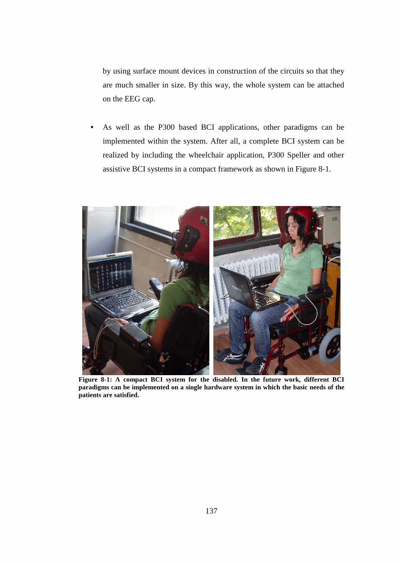
137
by using surface mount devices in construction of the circuits so that they
are much smaller in size. By this way, the whole system can be attached
on the EEG cap.
• As well as the P300 based BCI applications, other paradigms can be
implemented within the system. After all, a complete BCI system can be
realized by including the wheelchair application, P300 Speller and other
assistive BCI systems in a compact framework as shown in Figure 8-1.
Figure 8-1: A compact BCI system for the disabled. In the future work, different BCI paradigms can be implemented on a single hardware system in which the basic needs of the patients are satisfied.
138
REFERENCES
[1] Wolpaw J.R., Birbaumer N., McFarland D.J., Pfurtscheller G., Vaughan
T.M., “Brain Computer Interfaces for Communication and Control”, Clinical Neurophysiology, 113: 767-791, March 2002
[2] Lotte F., Congedo M., Lecuyer A., Lamarche F., Arnaldi B., “A Review of
Classification Algorithms for EEG-Based Brain-Computer Interfaces”, Journal of Neural Engineering, 4: R1-R13, January 2007
[3] Farwell L.A., Donchin E., “Talking off the top of your head: Toward a
Mental Prosthesis Utilizing Event-Related Brain Potentials”, Electroencephalography and Clinical Neurophysiology, 70: 510-523, 1988
[4] Kaper M., Meinicke P., Grossekathoefer U., Lingner T., Ritter H., “BCI
Competition 2003 – Dataset IIb: Support Vector Machines for the P300 Speller Paradigm” IEEE Transactions on Biomedical Engineering, Vol. 51, No. 6, June 2004
[5] Kaper M., Ritter H., “Progress in P300-based Brain-Computer
Interfacing”, IEEE International Workshop on Biomedical Circuits and Systems, 2004
[6] Rakotomamonjy A., Guigue V., “BCI Competition III: Dataset II –
Ensemble of SVMs for BCI P300 Speller”, IEEE Transactions on Biomedical Engineering, Vol.55, No.3, March 2008
[7] Bostanov V., “BCI Competition III - Data Sets Ib and IIb: Feature
Extraction From Event-Related Brain Potentials with the Continuous Wavelet Transform and the t-Value Scalogram”, IEEE Transactions on Biomedical Engineering, Vol. 51, No. 6, June 2004
139
[8] Xu N., Gao X., Hong B., Miao X., Gao S., “BCI Competition 2003 – Data Set IIb: Enhancing P300 Wave Detection Using ICA-based Subspace Projections for BCI Applications”, IEEE Transactions on Biomedical Engineering, Vol. 51, No. 6, June 2004
[9] Krusienski D.J., Sellers E.W., Cabestaing F., Bayoudh S., McFarland D.J.,
Vaughan T.M., Wolpaw J.R., “A Comparison of Classification Techniques for the P300 Speller”, Journal of Neural Engineering, 3: 299-305, 2006
[10] Guan J., Chen Y., Huang M., “Classification of Single-Trial Potentials
Evoked by Imitating-Natural-Reading Using v-SVM”, International Journal of Computational Intelligence Research, Vol.2, No.1: 110-114, 2006
[11] Guger C., Schlög A., Neuper C., Walterspacher D., Strein T., Pfurtscheller
G., “Rapid Prototyping of an EEG-Based Brain-Computer Interface (BCI)”, IEEE Transactions on Neural Systems and Rehabilitation Engineering, Vol.9, No. 1, March 2001
[12] Müller G.R., Neuper C., Pfurtscheller G., “Implementation of a
Telemonitoring System for the Control of an EEG-Based Brain-Computer Interface”, IEEE Transactions on Neural Systems and Rehabilitation Engineering, Vol.11, No. 1, March 2003
[13] Moore M.M., “Real-World Applications for Brain-Computer Interface
Technology” IEEE Transactions on Neural Systems and Rehabilitation Engineering, Vol.11, No. 2, June 2003
[14] Wolpaw J.R., McFarland D.J., Vaughan T.M., Schalk G., “The
Wadsworth Center Brain-Computer Interface (BCI) Research and Development Program”, IEEE Transactions on Neural Systems and Rehabilitation Engineering, Vol.11, No. 2, June 2003
[15] Schalk G., McFarland D.J., Hinterberger T., Birbaumer N., Wolpaw J.R.,
“BCI2000: A General-Purpose Brain-Computer Interface (BCI) System”, IEEE Transactions on Biomedical Engineering, Vol. 51, No. 6, June 2004

140
[16] Fabiani M., Gratton G., Karis D., Donchin E., “The Definition, Identification and Reliability of Measurements of the P300 component of the Event-Related Brain Potential”, Advances in Psychophysiology, Vol. 2 JAI Press, 1988
[17] Blankertz B., Müller K.R., Curio G., Vaughan T.M., Schalk G., Wolpaw
J.R., Schlögl A., Neuper C., Pfurtscheller G., Hinterberger T., Schröder M., Birbaumer N., “The BCI Competition 2003: Progress and Perspectives in Detection and Discrimination of EEG Single Trials”, IEEE Transactions on Biomedical Engineering, Vol.51, No.6, June 2004
[18] Blankertz B., BCI Competition II (2003) – P300 Speller Dataset
(webpage). Available online at: http://www.bbci.de/competition/ii/ , Documentation: http://www.bbci.de/competition/ii/albany_desc/albany_desc_ii.pdf
[19] Blankertz B., Müller K.R., Krusienski D.J., Schalk G., Wolpaw J.R., Schlögl A., Pfurtscheller G., Millan J.R., Schröder M., Birbaumer N., “The BCI Competition III: Validating Alternative Approaches to Actual BCI Problems”, IEEE Transactions on Neural Systems and Rehabilitation Engineering, Vol.14, No.2, June 2006
[20] Blankertz B., BCI Competition III (2005) – P300 Speller Dataset (webpage). Available online at: http://www.bbci.de/competition/iii/ , Documentation: http://bbci.de/competition/iii/desc_II.pdf
[21] Lin Z.L., Zhang C.S., “Enhancing Classification by Perceptual
Characteristics for the P300 Speller Paradigm”, Proceedings of the 2nd International IEEE EMBS Conference on Neural Engineering – Arlington/Virginia – March 16-19, 2005
[22] Thulasidas M., Guan C., Wu J., “Robust Classification of EEG Signals for
Brain-Computer Interface”, IEEE Transactions on Neural Systems and Rehabilitation Engineering, Vol. 14, No. 1, 2006
[23] Garrett D., Peterson D.A., Anderson C.W., Thaut M.H., “Comparison of
Linear, Nonlinear, and Feature Selection Methods for EEG Signal Classification”, IEEE Transactions on Neural Systems and Rehabilitation Engineering, Vol. 11, 141-4, 2003

141
[24] Blankertz B., Curio G., Müller K.R., “Classifying Single Trial EEG:
Towards Brain Computer Interfacing”, Advanced. Neural Information Processing Systems, Vol. 14, 157-64
[25] Schlögl A., Lee F., Bischof H., Pfurtscheller G., “Characterization of
Four-Class Motor Imagery EEG Data for the BCI-competition 2005”, Journal of Neural Engineering, Vol. 2, L14-22, 2005
[26] Zhang H., Guan C., Wang C., “A Statistical Model of Brain Signals with
Application to Brain-Computer Interface”, Proceedings of the 2005 IEEE, Engineering in Medicine and Biology 27th Annual Conference, Shanghai, China, September 1-4, 2005
[27] Hoffman U., “Bayesian Machine Learning Applied in a Brain Computer
Interface for Disabled Users”, Doctoral Thesis, École Polytechnique Federale De Lausanne, 2007
[28] Hoffmann U., Vesin J-M., Ebrahimi T., Diserens K., “An Efficient P300-
Based Brain-Computer Interface for Disabled Subjects”, Journal of Neuroscience Methods, 167, pp:115-125, 2008
[29] Hoffmann U., Garcia G.N., Vesin J-M., Ebrahimi T., “Application of the
Evidence Framework to Brain-Computer Interfaces”, In: Proceedings of the IEEE Engineering in Medicine and Biology Conference, (2004),
[30] Liu Y., Zhou Z., Hu D., Dong G., “T-weighted Approach for Neural Information Processing in P300 based Brain-Computer Interface”. International Conference on Neural Networks and Brain, 2005, Vol.3, pp.1535-1539, 13-15 October. 2005
[31] Serby H., Yom-Tov E., Inbar G.F., “An Improved P300-Based Brain-
Computer Interface”, IEEE Transactions on Neural Systems and Rehabilitation Engineering, Vol. 13, No. 1, March 2005
[32] Hayes M.H., “Statistical Digital Signal Processing and Modeling”, John
Wiley & Sons, Inc., 1996
142
[33] Therrien C.W., “Discrete Random Signals and Statistical Signal
Processing”, Prentice Hall Signal Processing Series, 1992 [34] Duda R.O., Hart P.E., “Pattern Classification and Scene Analysis”, John
Wiley & Sons, Inc., 1973 [35] Bishop C.M., “Neural Networks for Pattern Recognition”, Clerdon Press-
Oxford, 1995 [36] Vapnik V., “The Nature of Statistical Learning Theory”, Springer-Verlag,
New York, 1995 [37] Vapnik V., “Statistical Learning Theory”, John Wiley and Sons, Inc., New
York, 1998
[38] Burges C.J.C., “A Tutorial on Support Vector Machines for Pattern Recognition”, Data Mining Knowledge Discovery, Vol. 2, pp: 121-167, 1998.
[39] Cortes C., Vapnik V., “Support-Vector Network”, Machine Learning, Vol.
20, pp:273–297, 1995
[40] Schölkopf B., Smola A., Müller K.R., “Nonlinear Component Analysis as a Kernel Eigenvalue Problem”, Neural Computation, 10(5): 1299–1319, 1998
[41] Malmivuo J., Plonsey R., “Bioelectromagnetism – Principles and
Applications of Bioelectric and Biomagnetic Fields”, [Online book], Chapter 13, Available at: http://www.bem.fi/book/13/13.htm#03
[42] Guger C., “Brain Computer Interface”, Lecture notes in The 4th
International Summer School on Emerging Technologies in Biomedicine: Advanced Methods for the Estimation of Human Brain Activity and Connectivity, Applications to Rehabilitation Engineering, Patras, Greece, 29 June – 4 July 2008. http://heart.med.upatras.gr/school2008/Materials.html
143
[43] Jasper H.H. The ten-twenty electrode system of the International Federation. Electroencephalogr. Clinical Neurophysiology, (10) pp:370-375. 1958
[44] Wolpaw J.R, “Brain-Computer Interface Technology: A Review of the
First International Meeting”, IEEE Transactions on Rehabilitation Engineering, 8(2):164–173, 2000
[45] Kübler A., Mushahwar V.K., Hochberg L.R., Donoghue J.P., “BCI
Meeting 2005 – Workshop Clinical Issues and Applications”, IEEE Transactions on Neural Systems and Rehabilitation Engineering, Vol. 14, No.2, June 2006
[46] Mason S.G., Birch G.E., “A General Framework for Brain-Computer
Interface Design”, IEEE Transactions on Neural Systems and Rehabilitation Engineering, Vol. 11, No. 1, March 2003
[47] Cincotti F., Bianchi L., Birch G., Guger C., Mellinger J., Scherer R.,
Schmidt R.N., Suarez O.Y., Schalk G., “BCI Meeting 2005 – Workshop on Technology: Hardware and Software”, IEEE Transactions on Neural Systems and Rehabilitation Engineering, Vol. 14, No.2, June 2006
[48] EEG systems: http://archlab.gmu.edu/people/cbaldwi4/EEG.jpg [49] Mobile EEG systems: http://www.gtec.at/content.htm [50] Leuthardt E.C., Miller K.J., Schalk G., Rao R.P.N., Ojemann J.G.,
“Electrocorticography-Based Brain Computer Interface – The Seattle Experience”, IEEE Transactions on Neural Systems and Rehabilitation Engineering, Vol. 14, No.2, June 2006
[51] Wilson J.A., Felton E.A., Garell P.C., Schalk G., Williams J.C., “ECoG
Factors Underlying Control of a Brain-Computer Interface”, IEEE Transactions on Neural Systems and Rehabilitation Engineering, Vol. 14, No.2, June 2006
[52] Hill N.J., Lal T.N., Schröder M., Hinterberger T., Wilhelm B., Nijboer F.,
Mochty U., Widman G., Elger C., Schölkopf B., Kübler A., Birbaumer N., “Classifying EEG and ECoG Signals Without Subject Training for Fast BCI Implementation: Comparison of Nonparalyzed and Completely Paralyzed Subjects”, IEEE Transactions on Neural Systems and Rehabilitation Engineering, Vol. 14, No.2, June 2006
[53] Thakor N.V., “Frontiers of Neuroengineering”, Lecture notes in The 4th
International Summer School on Emerging Technologies in Biomedicine:

144
Advanced Methods for the Estimation of Human Brain Activity and Connectivity, Applications to Rehabilitation Engineering, Patras, Greece, 29 June – 4 July 2008. http://heart.med.upatras.gr/school2008/Materials.html
[54] Lebedev M.A., Nicoleis M.A., “Brain-machine interfaces: Past, present
and future”, Trends in Neurosciences, Vol.29, No.9, pp: 536-546, September 2006.
[55] Magnetoencephalography - SQUID, http://en.wikipedia.org/wiki/SQUID [56] Lal T.N., Schröder M, Hill N.J., Preissl H., Hinterberger T., Mellinger J.,
Rosenstiel W., Birbaumer N., Hofmann T., Schölkopf B., “A Brain-Computer Interface with Online Feedback Based on Magnetoencephalography”, Proceedings of the 22nd International Conference on Machine Learning, Bonn, Germany, 2005
[57] Kauhanen L., Nykopp T., Lehtonen J., Jylanki P., Heikkonen J., Rantanen
P., Alaranta H., Sams M., “EEG and MEG Brain-Computer Interface for Tetraplegic Patients”, IEEE Transactions on Neural Systems and Rehabilitation Engineering, Vol.14, No.2, pp.190-193, June 2006
[58] The picture of a commercial Magnetoencephalographm.
http://www.elekta.com/assets/functional_mapping/images/meg_side.jpg
[59] Weiskopf N., Mathiak K., Bock S.W., Scharnowski F., Veit R., Grodd W., Goebel R., Birbaumer N., “Principles of a Brain-Computer Interface (BCI) Based on Real-Time Functional Magnetic Resonance Imaging (fMRI)”, IEEE Transactions on Biomedical Engineering, Vol.51, No.6, June 2004
[60] Choi, S.H., Lee M., “Brain Computer Interface Using EEG Sensors Based
on an fMRI Experiment”, In International Joint Conference on Neural Networks, Vancouver, Canada, July 2006
[61] Choi, S.H., Lee M., Wang Y., Hong B., “Estimation of Optimal Location
of EEG Reference Electrode for Motor Imagery Based BCI Using fMRI”, Proceedings of the 28th IEEE EMBS Annual International Conference, New York, USA, August 2006
[62] Coyle S., Ward T., Markham C., McDarby G., “On the Suitability of
Near-Infrared (NIR) Systems for Next-Generation Brain-Computer Interfaces”, Physiological Measurement, Vol. 25, pp. 815–822, August 2004
[63] Wolpaw J.R., Loeb G.E., Allison B.Z., Donchin E., Nascimento O.F.D.,
Heetderks W.J., Nijboer F., Shain W.G., Turner J.N., “BCI Meeting 2005
145
– Workshop on Signals and Recording Methods”, IEEE Transactions on Neural Systems and Rehabilitation Engineering, Vol. 14, No.2, June 2006
[64] Gao X., Xu D., Cheng M., Gao S., “A BCI-Based Environmental
Controller for the Motion-Disabled”, IEEE Transactions on Neural Systems and Rehabilitation Engineering, Vol. 11, No.2, June 2003
[65] Maggi L., Parini S., Piccini L., Panfili G., Adreoni G., “A Four Command
BCI System Based on the SSVEP Protocol”, In Proceedings of the 28th IEEE EMBS Annual International Conference, New York, USA, August 2006
[66] Nielsen K.D., Cabrera A.F., Nascimento O.F.D., “EEG Based BCI—
Towards a Better Control. Brain-Computer Interface Research at Aalborg University”, IEEE Transactions on Neural Systems and Rehabilitation Engineering, Vol. 14, No.2, June 2006
[67] Pfurtscheller G., Neuper C., “Motor Imagery and Direct Brain-Computer
Communication”, Proceedings of the IEEE , Vol.89, No.7, pp.1123-1134, July 2001
[68] Townsend G., Graimann B., Pfurtscheller G., “Continuous EEG
Classification During Motor Imagery—Simulation of an Asynchronous BCI”, IEEE Transactions on Neural Systems and Rehabilitation Engineering, Vol. 12, No.2, June 2004
[69] Curran E., Sykacek P., Stokes M., Roberts S., Penny W., Johnsrude I.,
Owen A., “Cognitive Tasks for Driving a Brain-Computer Interfacing System: A Pilot Study”, IEEE Transactions on Neural Systems and Rehabilitation Engineering, Vol.12, No.1, pp.48-54, March 2004
[70] Pfurtscheller G., “Event-related desynchronization (ERD) and event
related synchronization (ERS),” In Electroencephalography: Basic Principles, Clinical Applications and Related Fields, 4th ed., E. Niedermeyer and F. H. Lopes da Silva, Eds. Baltimore, MD: Williams & Wilkins, 1999, pp. 958–967
[71] Pfurtscheller G., da Silva F.H.L, “Functional Meaning of Event-Related
Desynchronization (ERD) and Synchronization (ERS),” In Event-Related Desynchronization, Handbook of Electroenceph. and Clin. Neurophysiol., rev ed,. Amsterdam, The Netherlands: Elsevier, 1999, Vol. 6, pp. 51–65
[72] Lalor E.C., Kelly S.P., Finucane C., Burke R., Smith R., Reilly R.B.,
McDarby G., “Steady-state VEP-based brain-computer interface control in an immersive 3D gaming environment”, EURASIP Journal on Applied Signal Processing, (19):3156–3164, 2005

146
[73] OpenVIBE, A Software for Brain Computer Interfaces and Real Time
Neurosciences, Webpage: http://openvibe.inria.fr/ [74] Electroencephalogram: http://en.wikipedia.org/wiki/Electroencephalogram [75] Control of a wheelchair with BCI
http://www.utar.edu.my/ipsr/img/brain3.JPG [76] Control of a robotic arm with BCI
http://en.wikipedia.org/wiki/File:Monkey_using_a_robotic_arm.jpg [77] Chang C.-C., Lin C.-J., “LIBSVM: A Library for Support Vector
Machines”. Online available at: http://www.csie.ntu.edu.tw/~cjlin/libsvm/ [78] Uşaklı A.B., Gençer N.G., “USB-Based 256-Channel
Electroencephalographic Data Acquisition System for Electrical Source Imaging of the Human Brain”, Instrumentation Science and Technology, 35: 255-273, 2007
[79] Microchip Technology Inc., “PIC18F2458/2553/4458/4553 Datasheet,
28/40/44-Pin High-Performance, Enhanced Flash, USB Microcontrollers with 12-Bit A/D and nanoWatt Technology”. Available at: ww1.microchip.com/downloads/en/DeviceDoc/39887b.pdf
[80] Vishay Semiconductors, “IL300, Linear Optocoupler, High Gain Stability,
Wide Bandwidth”, Documentation: http://www.vishay.com/docs/83622/83622.pdf
[81] Compumedics – Neuroscan, Quik-Caps,
http://www.neuroscan.com/cart/Details.cfm?ProdID=188&category=6 [82] Erdoğan H.B., “A 10 channel EEG system for BCI applications, Technical
Documentation”, Electrical and Electronics Engineering Dept., Brain Research Laboratory, METU, will be available at: http://www.eee.metu.edu.tr/~biomed/brl/index.html
[83] Webster J.G., “Medical Instrumentation: Application and Design”, John
Wiley and Sons Inc., 3rd ed. 1997

147
APPENDIX A
PROOF OF WIDE SENSE STATIONARITY OF A
SINUSOIDAL RANDOM PROCESS
A random process ( )nx is said to be a wide-sense stationary process if the
following conditions are satisfied [32]:
1. The mean of the process ( )nxµ is a constant.
2. The autocorrelation ( )21,nnRx is a function of ( )21 nn − .
Consider the random process given by
( ) ii njw
iieAnx ϕ+∑= (B.1)
where iA ’s and iw ’s are deterministic (amplitude and frequency) parameters
defining the sinusoid. Here, the phase parameters iϕ ’s are random variables
whose distribution is assumed to be uniform between 0 and π2 . That is,
≤≤=
elsewheref i
ii
0
202
1)(
πϕπϕϕ (B.2)

148
Proof of Condition 1
{ }
{ }
434210
2
0
2
0
)(
)(
2
1
2
1
)(
)()(
=
=
∞+
∞−
+
+
=
=
=
=
=
=
∑
∫∑
∫∑
∑
∑
π
ϕϕ
πϕ
ϕϕ
ϕ
ϕ
π
ϕπ
ϕϕ
µ
i
ii
ii
i
ii
ii
ii
jnjw
ii
ijnjw
ii
iijnjw
ii
nwj
ii
nwj
ii
x
eeA
deeA
dfeeA
eEA
eAE
nxEn
(B.3)
( ) 0=⇒ nxµ
It can be seen that the mean of the random process is constant. Therefore, the first
condition for WSS is satisfied.
Proof of Condition 2
( ) ( ) ( ){ }( ) ( ) ( )∫ ∑∑
=
=
+−+NN
nwj
kk
nwj
ii
x
ddfeAeA
nxnxEnnR
N
kkii ϕϕϕϕϕϕϕϕ ...,...,
,
11,...,
2*
121
1
21 (B.4)
Here, it can be assumed that iϕ ’s are independent random variables so that their
joint probability density can be represented as a product of their marginal
densities:
( ) ( ) ( ) ( )NN NNffff ϕϕϕϕϕ ϕϕϕϕϕ ........,..., 211,..., 211
= (B.5)

149
( )( ) ( ) ( ) ( ) ( )∫ ∑∑
=⇒
+−+NN
nwj
kk
nwj
ii
x
ddfffeAeA
nnR
N
kkii ϕϕϕϕϕ ϕϕϕϕϕ ......
,
121
21
21
21 (B.6)
One can note from the above expression that the integral of the cross-
multiplication of exponential terms yields to 0 unless ki ≠ . That is,
( ) ( ) ( ) ( )
02
1
......
0
2
0
)(
2
0
11
21
1
21
=
=
=
−−
+−+
∫
∫
43421
πϕϕ
π
ϕϕϕϕ
π
ϕϕϕϕ
kiki
N
kkii
jN
njwnjwki
NNnwjnwj
ki
eeeAA
ddffeeAA
(B.7)
Therefore,
( ) ( ) ( ) ( ) ( )
( )∑
∑ ∫
−
=
−−
=
=⇒
i
nnjwN
i
iNN
jnnjwix
i
N
iii
eA
ddffeeAnnR
21
1
21
2
1
......,
2
2
0
111
221
π
ϕϕϕϕπ
ϕϕϕϕ321
(B.8)
which is a function of )( 21 nn − . Therefore, ( )nx is WSS process as it also
satisfies the second condition.
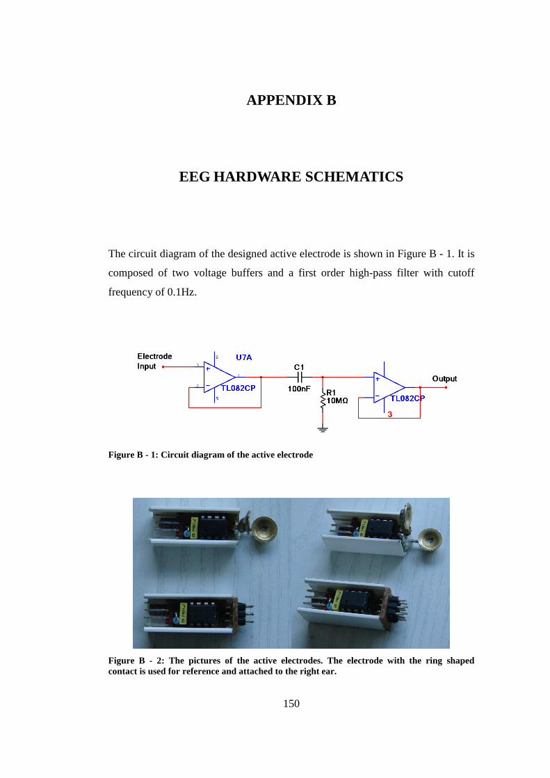
150
APPENDIX B
EEG HARDWARE SCHEMATICS
The circuit diagram of the designed active electrode is shown in Figure B - 1. It is
composed of two voltage buffers and a first order high-pass filter with cutoff
frequency of 0.1Hz.
Figure B - 1: Circuit diagram of the active electrode
Figure B - 2: The pictures of the active electrodes. The electrode with the ring shaped contact is used for reference and attached to the right ear.

151
The EEG signals are amplified differentially with the preamplification stage in
which the differential gain is adjusted to 50. The output signal is filtered to
remove the DC offsets. The circuit diagram of the preamplifier circuitry is given
in Figure B - 3.
Figure B - 3: The preamplifier circuitry in the EEG amplifier.
Two active filters are used in the analog circuitry. The amplified signal is first
filtered with a band-stop filter with frequency of 50Hz to remove the effect of the
power line noise and after the notch filter, the signal is processed with a third
order low-pass filter to remove the unnecessary components in the EEG
frequency range. For this purpose, the cut-off frequency of the low-pass filter is
set to 40Hz. The filter is designed according to Bessel filter specifications to
obtain a flat group delay for all frequencies in the range. The circuit diagrams of
the filter circuits are given in Figure B - 4 and Figure B - 5.
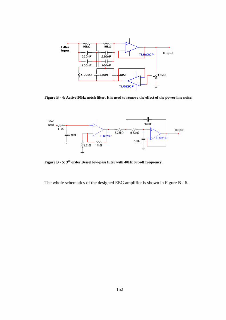
152
Figure B - 4: Active 50Hz notch filter. It is used to remove the effect of the power line noise.
Figure B - 5: 3rd order Bessel low-pass filter with 40Hz cut-off frequency.
The whole schematics of the designed EEG amplifier is shown in Figure B - 6.
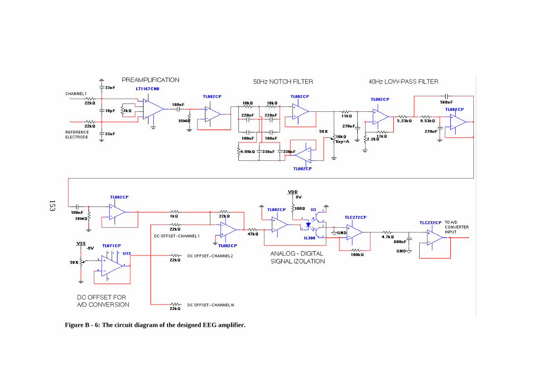
153
Figure B - 6: The circuit diagram of the designed EEG amplifier.
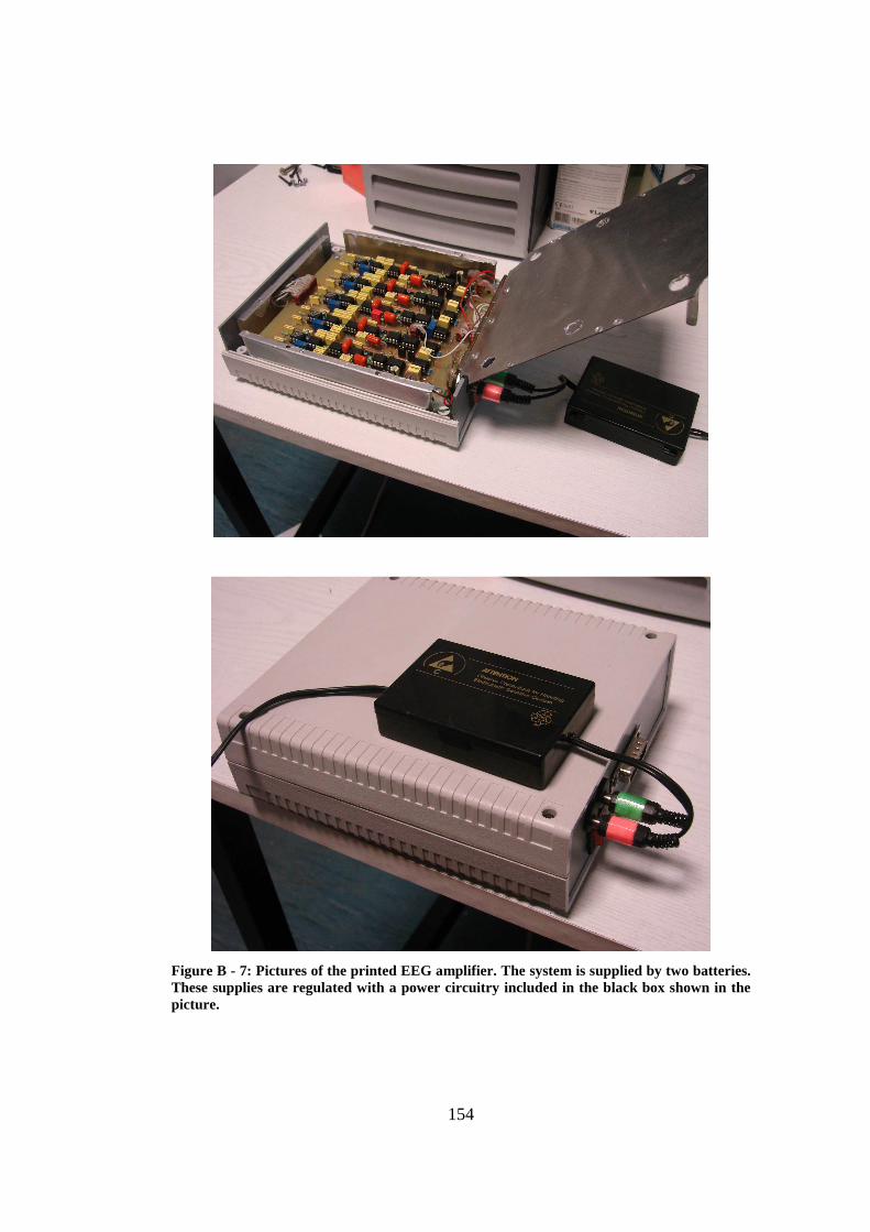
154
Figure B - 7: Pictures of the printed EEG amplifier. The system is supplied by two batteries. These supplies are regulated with a power circuitry included in the black box shown in the picture.
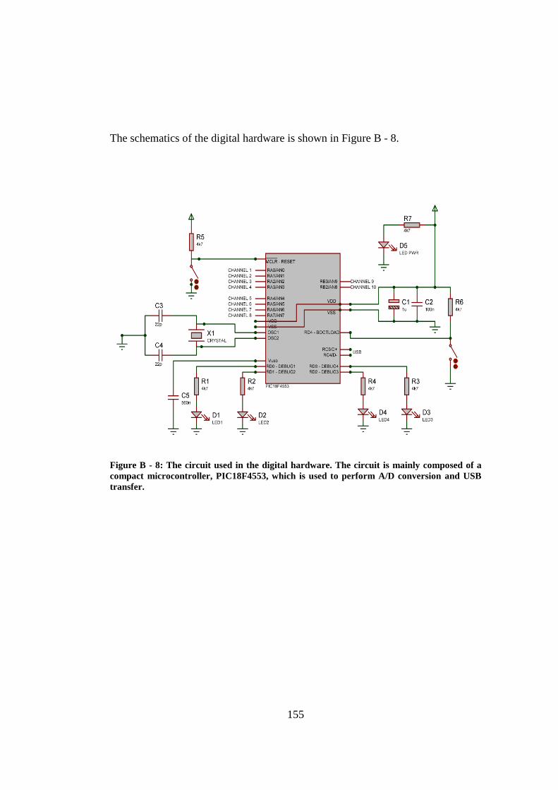
155
The schematics of the digital hardware is shown in Figure B - 8.
Figure B - 8: The circuit used in the digital hardware. The circuit is mainly composed of a compact microcontroller, PIC18F4553, which is used to perform A/D conversion and USB transfer.
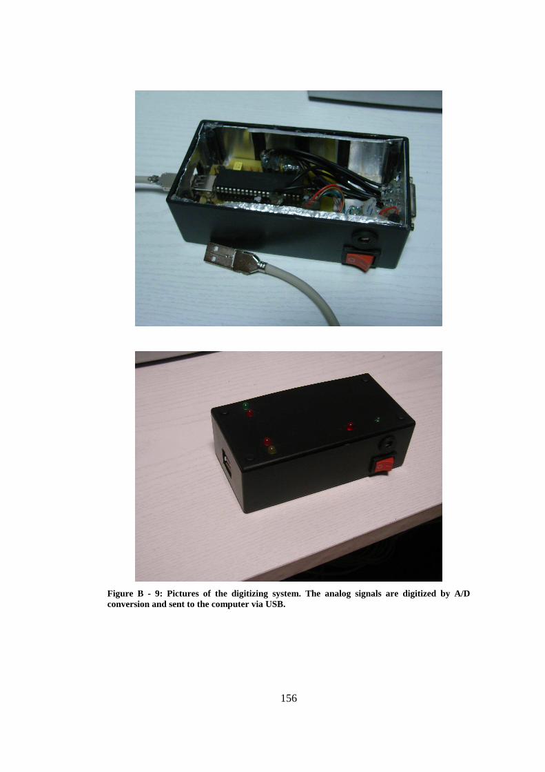
156
Figure B - 9: Pictures of the digitizing system. The analog signals are digitized by A/D conversion and sent to the computer via USB.
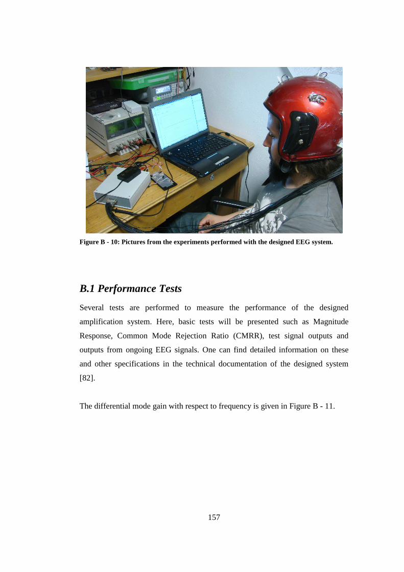
157
Figure B - 10: Pictures from the experiments performed with the designed EEG system.
B.1 Performance Tests
Several tests are performed to measure the performance of the designed
amplification system. Here, basic tests will be presented such as Magnitude
Response, Common Mode Rejection Ratio (CMRR), test signal outputs and
outputs from ongoing EEG signals. One can find detailed information on these
and other specifications in the technical documentation of the designed system
[82].
The differential mode gain with respect to frequency is given in Figure B - 11.
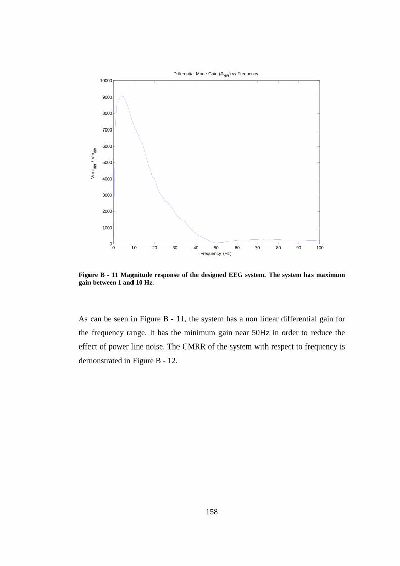
158
0 10 20 30 40 50 60 70 80 90 1000
1000
2000
3000
4000
5000
6000
7000
8000
9000
10000
Frequency (Hz)
Vou
t diff
/ V
indi
ff
Differential Mode Gain (Adiff) vs Frequency
Figure B - 11 Magnitude response of the designed EEG system. The system has maximum gain between 1 and 10 Hz.
As can be seen in Figure B - 11, the system has a non linear differential gain for
the frequency range. It has the minimum gain near 50Hz in order to reduce the
effect of power line noise. The CMRR of the system with respect to frequency is
demonstrated in Figure B - 12.
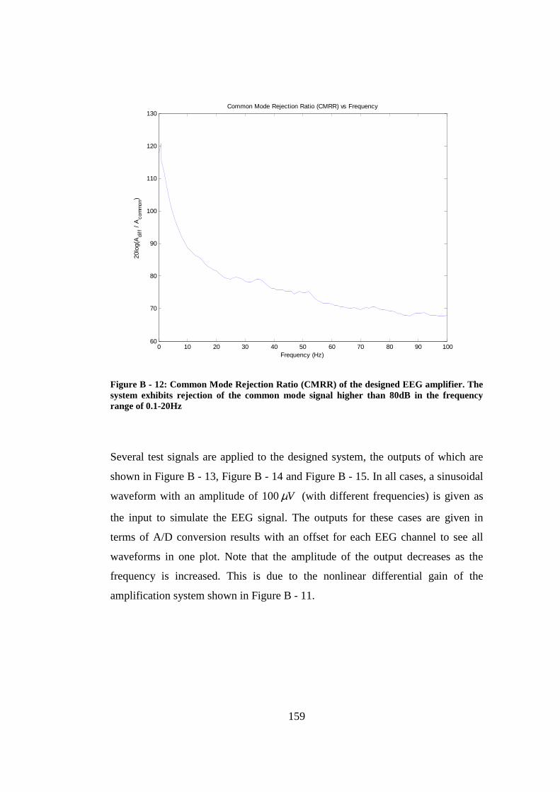
159
0 10 20 30 40 50 60 70 80 90 10060
70
80
90
100
110
120
130
Frequency (Hz)
20lo
g(A
diff
/ A
com
mon
)
Common Mode Rejection Ratio (CMRR) vs Frequency
Figure B - 12: Common Mode Rejection Ratio (CMRR) of the designed EEG amplifier. The system exhibits rejection of the common mode signal higher than 80dB in the frequency range of 0.1-20Hz
Several test signals are applied to the designed system, the outputs of which are
shown in Figure B - 13, Figure B - 14 and Figure B - 15. In all cases, a sinusoidal
waveform with an amplitude of 100Vµ (with different frequencies) is given as
the input to simulate the EEG signal. The outputs for these cases are given in
terms of A/D conversion results with an offset for each EEG channel to see all
waveforms in one plot. Note that the amplitude of the output decreases as the
frequency is increased. This is due to the nonlinear differential gain of the
amplification system shown in Figure B - 11.
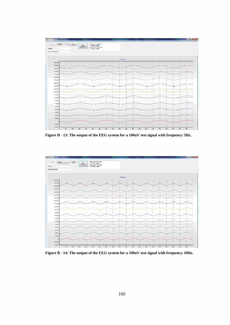
160
Figure B - 13: The output of the EEG system for a 100uV test signal with frequency 5Hz.
Figure B - 14: The output of the EEG system for a 100uV test signal with frequency 10Hz.
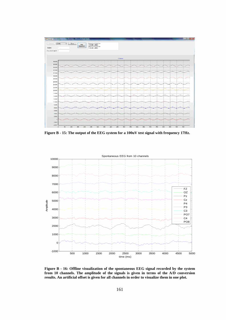
161
Figure B - 15: The output of the EEG system for a 100uV test signal with frequency 17Hz.
500 1000 1500 2000 2500 3000 3500 4000 4500 5000-1000
0
1000
2000
3000
4000
5000
6000
7000
8000
9000
10000
time (ms)
Am
plitu
de
Spontaneous EEG from 10 channels
FZOZ
Pz
Cz
P4P3
C3
PO7
C4PO8
Figure B - 16: Offline visualization of the spontaneous EEG signal recorded by the system from 10 channels. The amplitude of the signals is given in terms of the A/D conversion results. An artificial offset is given for all channels in order to visualize them in one plot.


![An embedded implementation based on adaptive filter bank for brain-computer interface … · 2018-05-08 · bank for brain-computer interface systems Author: ... (ERP) [3], and P300](https://img.pdfslide.us/doc/110x75/5f75f7d5855c0a7b2537e92e/an-embedded-implementation-based-on-adaptive-filter-bank-for-brain-computer-interface.jpg)