Embed Size (px)
Citation preview

A DEFECT CORRECTION METHOD FOR THE TIME-DEPENDENTNAVIER-STOKES EQUATIONS
A. LABOVSCHII1,2 ∗
Abstract. A method for solving the time dependent Navier-Stokes equations, aiming at higherReynolds’ number, is presented. The direct numerical simulation of flows with high Reynolds’ numberis computationally expensive. The method presented is unconditionally stable, computationallycheap and gives an accurate approximation to the quantities sought. In the defect step, the artificialviscosity parameter is added to the inverse Reynolds number as a stability factor, and the system isantidiffused in the correction step. Stability of the method is proven, and the error estimations forvelocity and pressure are derived for the one- and two-step defect-correction methods. The spacialerror is O(h) for the one-step defect-correction method, and O(h2) for the two-step method, where his the diameter of the mesh. The method is compared to an alternative approach, and both methodsare applied to a singularly perturbed convection-diffusion problem. The numerical results are given,which demonstrate the advantage (stability, no oscillations) of the method presented.
Key words. Navier-Stokes, defect-correction, time-dependent, artificial viscosity, residual, an-tidiffuse, Reynolds number.
∗Department of Mathematics, University of [email protected], http://www.pitt.edu/∼ayl22Partially supported by NSF Grant DMS-0508260
1
2
1. Introduction. In the numerical solution of higher Reynolds number flowproblems one of the most commonly reported results is that ”the method failed”. Of-ten ”failure” means that the iterative method used to solve the linear and/or nonlinearsystem for the approximate solution at the new time level failed to converge withinthe time constraints of the problem or the resulting approximation had poor solutionquality. The first type of failure can usually be overcome easily by using an upwind orartificial viscosity (AV) discretization at the expense of decreasing dramatically theaccuracy of the method and possibly even altering the predictions of the simulationat the qualitative, O(1) level, therefore increasing the likelihood of the second type offailure.
One interesting approach to attaining (by a convergent method) an approximatesolution of desired accuracy is the defect correction method (DCM). Briefly, let akth order accurate discretization of the equilibrium Navier-Stokes equations (NSE) bewritten as
NSEh(uh) = f, (1.1)
The DCM computes uh1 , ..., uh
k as
−αh∆huh1 + NSEh(uh
1 ) = f, (1.2)−αh∆huh
l + NSEh(uhl ) = f − αh∆huh
l−1, for l = 2, ..., k,
where the velocity approximations uhi are sought in the finite element space of piece-
wise polynomials of degree k.It has been proven under quite general conditions (see, e.g., [LLP02]) that for the
intermediate approximations of the equilibrium NSE
‖uNSE − uhl ‖energy−norm = O(hk + h‖uNSE − uh
l−1‖energy−norm) = O(hk + hl),
and thus, after l = k steps,
‖u− uhk‖energy−norm = O(hk).
Note that (1.2) requires solving an AV approximation k times which is often cheaperand more reliable than solving (1.1) once.
In problems with high Reynolds number we may expect turbulence. In that casethe DCM needs to be combined with appropriate turbulence models. These modelstend to introduce extra nonlinearities (due to the closure of the model); it might bepossible to incorporate them into the residual on the right-hand side, as was done inthe quasistatic case by Ervin, Layton, Maubach [ELM00].
There has been an extensive study and development of this approach for equilib-rium flow problems, see e.g. Hemker[Hem82], Koren[K91], Heinrichs[Hei96], Layton,Lee, Peterson[LLP02], Ervin, Lee[EL06], and subsection 1.1 for a review of this work.
For many years, it has been widely believed that (1.2) can be directly importedinto implicit time discretizations of flow problems in the obvious way: discretize intime, given uh(tOLD), the quasistatic flow problem for uh(tNEW ) is solved by applying(1.2) directly, resulting in
−αh∆huh1 (tNEW ) + B(uh
1 (tNEW ), uhk(tOLD)) + NSEh(uh
1 (tNEW )) = f, (1.3)−αh∆huh
l (tNEW ) + B(uhl (tNEW ), uh
k(tOLD)) + NSEh(uhl (tNEW ))
= f − αh∆huhl−1(tNEW ), for l = 2, ..., k,
3
where B is a time stepping operator (e.g., Backward Euler), and k is the degree ofpiecewise polynomials in the finite element space.
Unfortunately, this natural idea doesn’t seem to be even stable (see Section 7).On the other hand, there is a parallel development of DCM’s, for initial value
problems in which no spacial stabilization (such as −αh∆h in (1.2)) is used, butDCM is used to increase the accuracy of the time discretization. This work contains noreports of instabilities: see, e.g., Heywood, Rannacher[HR90], Hemker, Shishkin[HSS],Lallemand, Koren[LK93], Minion[M04]. Yet, in spite of this parallel development andafter 30+ years of studies of (1.2), there has yet to be a successful extension of (1.2)to time dependent flow problems.
This report will present this extension of (1.2) to the time dependent problem. Wenotice that the obvious extension, described above, is in fact unstable, see Section 7 .We give a small but critically important modification of the above natural extensionto time dependent problems, that we prove to be unconditionally stable (Theorem 3.3)and convergent (Theorem 4.3). We complement the stability proof of the modifiedDCM by a complete error analysis, which confirms the expected error in the resultingmethod: ‖u(tn)− uh
l (tn)‖energy−norm = O(∆ta + hk + hl), l = 1, ..., k, where a is theorder of accuracy of the (implicit) time stepping employed.
The error analysis is necessarily technical. To keep the details under some control,we study the backward Euler time discretization (It will be clear from our analysisthat extension to more accurate time discretizations requires no new ideas and onlymore pages).
In subsection 1.1 we review important previous work on DCM in space and DCMin time. Section 2 begins with (the inevitable) notation and preliminaries. Section3, the heart of the report, gives the stability proof. The error analysis is given inSections 4, 5.2 and Section 7 gives a numerical illustration.
Consider the time dependent, incompressible Navier-Stokes equations
∂u
∂t−Re−1∆u + u · ∇u +∇p = f, for x ∈ Ω, 0 < t ≤ T, (1.4)
∇ · u = 0, x ∈ Ω, 0 < t ≤ T,
u(x, 0) = u0(x), x ∈ Ω,
u|∂Ω = 0, for 0 < t ≤ T,
where Ω ⊂ Rd, d = 2, 3.
Before proceeding with the analysis we shall present carefully next the preciseextension of (1.2) to the time dependent NSE that we study.
Let Xh ⊂ X, Qh ⊂ Q be finite-dimensional finite element spaces. Denote thefinite-element discretization of the Navier-Stokes operator by
NhRe(u, p) ≡ ∂u
∂t−Re−1∆hu + (u · ∇h)u +∇hp.
Adding an artificial viscosity parameter to the inverse Reynolds number leads to themodified Navier-Stokes operator
NhRe
(u, p) ≡ ∂u
∂t− (h + Re−1)∆hu + (u · ∇h)u +∇hp.
The method proceeds as follows: first we compute the AV approximation (u1, p1)∈ (Xh, Qh) via
NhRe
(u1, p1) = f.

4
The accuracy of the approximation is then increased by the correction step: compute(u2, p2) ∈ (Xh, Qh), satisfying
NhRe
(u2, p2)−NhRe
(u1, p1) = f −NhRe(u1, p1).
The Backward Euler time discretization, combined with the two-step defect cor-rection method in space leads to the following system of equations for (uh,n+1
1 , ph,n+11 ),
(uh,n+12 , ph,n+1
2 ) ∈ (Xh, Qh), ∀vh ∈ Xh at t = tn+1, n ≥ 0, with k := ∆t = ti+1 − ti
(uh,n+1
1 − uh,n1
k, vh) + (h + Re−1)(∇uh,n+1
1 ,∇vh) + b∗(uh,n+11 , uh,n+1
1 , vh) (1.5)
−(ph,n+11 ,∇ · vh) = (f(tn+1), vh),
(uh,n+1
2 − uh,n2
k, vh) + (h + Re−1)(∇uh,n+1
2 ,∇vh) + b∗(uh,n+12 , uh,n+1
2 , vh)
−(ph,n+12 ,∇ · vh) = (f(tn+1), vh) + h(∇uh,n+1
1 ,∇vh),
where b∗(·, ·, ·) is the explicitely skew-symmetrized trilinear form, defined below.The initial value approximations are taken to be uh,0
1 = uh,02 = us
0, where us0 is
the modified Stokes projection of u0 onto the space V h of discretely divergence-freefunctions (this projection and this space are defined in section 2). The stability anderror estimate for the modified Stokes projection are proven in the sections 3 and 4.
1.1. Previous results. Many iterative methods can be written as a Defect Cor-rection method, see e. g. Bohmer, Hemker, Stetter [BHS]. In the DCM we consider,no iterates occur; a small number of updates are calculated to increase the accuracyof the velocity and pressure approximations. Thus it is most similar to DCM’s whichare close to Richardson extrapolation (see, for example, Mathews, Fink [MF04]).In the late 1970’s Hemker (Bohmer, Stetter, Heinrichs and others) discovered thatDCM, properly interpreted, is good also for nearly singular problems. Examples forwhich this has been successful include equilibrium Euler equations (Koren, Lallemand[LK93]), high Reynolds number problems (Layton, Lee, Peterson [LLP02]), viscoelas-tic problems (Ervin, Lee [EL06]).
There has also been interesting work on Spectral Deferred Correction (SDC) forIVP’s (e.g., Minion [M04], Bourlioux, Layton, Minion [BLM03], Kress, Gustafsson[KG02], Dutt, Greengard, Rokhlin [DGR00]). With the exception of the SDC meth-ods for time stepping, the majority of the results has been obtained for the equilibriumproblems - an odd fact, since, e.g., for the Euler equations the time-dependent prob-lem is natural. For example, it has not been known apparently if the natural idea oftime stepping combined with the DCM in space for the associated quasi-equilibriumproblem is stable.
2. Mathematical Preliminaries and Notations. Throughout this paper thenorm ‖ · ‖ will denote the usual L2(Ω)-norm of scalars, vectors and tensors, inducedby the usual L2 inner-product, denoted by (·, ·). The space that velocity (at time t)belongs to, is
X = H10 (Ω)d = v ∈ L2(Ω)d : ∇v ∈ L2(Ω)d×d and v = 0 on ∂Ω.
with the norm ‖v‖X = ‖∇v‖. The space dual to X, is equipped with the norm
‖f‖−1 = supv∈X
(f, v)‖∇v‖ .
5
The pressure (at time t) is sought in the space
Q = L20(Ω) = q : q ∈ L2(Ω),
∫
Ω
q(x)dx = 0.
Also introduce the space of weakly divergence-free functions
X ⊃ V = v ∈ X : (∇ · v, q) = 0, ∀q ∈ Q.
For measurable v : [0, T ] → X, we define
‖v‖Lp(0,T ;X) = (∫ T
0
‖v(t)‖pXdt)
1p , 1 ≤ p < ∞,
and
‖v‖L∞(0,T ;X) = ess sup0≤t≤T
‖v(t)‖X .
Define the trilinear form on X ×X ×X
b(u, v, w) =∫
Ω
u · ∇v · wdx.
The following lemma is also necessary for the analysisLemma 2.1. There exist finite constants M = M(d) and N = N(d) s.t. M ≥ N
and
M = supu,v,w∈X
b(u, v, w)‖∇u‖‖∇v‖‖∇w‖ < ∞ , N = sup
u,v,w∈V
b(u, v, w)‖∇u‖‖∇v‖‖∇w‖ < ∞.
The proof can be found, for example, in [GR79]. The corresponding constants Mh
and Nh are defined by replacing X by the finite element space Xh ⊂ X and V byV h ⊂ X, which will be defined below. Note that M ≥ max(Mh, N, Nh) and that ash → 0, Nh → N and Mh → M (see [GR79]).
Throughout the paper, we shall assume that the velocity-pressure finite elementspaces Xh ⊂ X and Qh ⊂ Q are conforming, have typical approximation propertiesof finite element spaces commonly in use, and satisfy the discrete inf-sup, or LBBh,condition
infqh∈Qh
supvh∈Xh
(qh,∇ · vh)‖∇vh‖‖qh‖ ≥ βh > 0, (2.1)
where βh is bounded away from zero uniformly in h. Examples of such spaces can befound in [GR79]. We shall consider Xh ⊂ X, Qh ⊂ Q to be spaces of continuouspiecewise polynomials of degree m and m − 1, respectively, with m ≥ 2. The caseof m = 1 is not considered, because the optimal error estimate (of the order h) isobtained after the first step of the method - and therefore the DCM in this case isreduced to the artificial viscosity approach.
The space of discretely divergence-free functions is defined as follows
V h = vh ∈ Xh : (qh,∇ · vh) = 0,∀qh ∈ Qh.
In the analysis we use the properties of the following Modified Stokes Projection
6
Definition 2.2 (Modified Stokes Projection). Define the Stokes projection op-erator PS: (X, Q) → (Xh, Qh), PS(u, p) = (u, p), satisfying
(h + Re−1)(∇(u− u),∇vh)− (p− p,∇ · vh) = 0, (2.2)(∇ · (u− u), qh) = 0,
for any vh ∈ V h, qh ∈ Qh.In (V h, Qh) this formulation reads: given (u, p) ∈ (X, Q), find u ∈ V h satisfying
(h + Re−1)(∇(u− u),∇vh)− (p− qh,∇ · vh) = 0, (2.3)
for any vh ∈ V h, qh ∈ Qh.Define the explicitly skew-symmetrized trilinear form
b∗(u, v, w) :=12(u · ∇v, w)− 1
2(u · ∇w, v).
The following estimate is easy to prove (see, e.g., [GR79]): there exists a constantC = C(Ω) such that
|b∗(u, v, w)| ≤ C(Ω)‖∇u‖‖∇v‖‖∇w‖. (2.4)
The proofs will require the sharper bound on the nonlinearity. This upper boundis improvable in R2.
Lemma 2.3 (The sharper bound on the nonlinear term). Let Ω ⊂ Rd, d = 2, 3.For all u, v, w ∈ X
|b∗(u, v, w)| ≤ C(Ω)√‖u‖‖∇u‖‖∇v‖‖∇w‖.
Proof. See [GR79].We will also need the following inequalities: for any u ∈ V
infv∈V h
‖∇(u− v)‖ ≤ C(Ω) infv∈Xh
‖∇(u− v)‖, (2.5)
infv∈V h
‖u− v‖ ≤ C(Ω) infv∈Xh
‖∇(u− v)‖. (2.6)
The proof of (2.5) can be found, e.g., in [GR79], and (2.6) follows from the Poincare-Friedrich’s inequality and (2.5).
Define also the number of time steps N := Tk .
We conclude the preliminaries by formulating the discrete Gronwall’s lemma, see,e.g. [HR90]
Lemma 2.4. Let k, B, and aµ, bµ, cµ, γµ, for integers µ ≥ 0, be nonnegativenumbers such that:
an + k
n∑µ=0
bµ ≤ k
n∑µ=0
γµaµ + k
n∑µ=0
cµ + B for n ≥ 0.
Suppose that kγµ < 1 for all µ, and set σµ = (1− kγµ)−1. Then
an + k
n∑µ=0
bµ ≤ ek∑n
µ=0 σµγµ · [kn∑
µ=0
cµ + B].
7
3. Stability of the Velocity. In this section we prove the unconditional sta-bility of the discrete artificial viscosity approximation uh
1 and use this result to provestability of the higher order approximation uh
2 . Over 0 ≤ t ≤ T < ∞ the approxima-tions uh
1 and uh2 are bounded uniformly in Re.
Hence, the formulation (1.5) gives the unconditionally stable extension of thedefect correction method to the time-dependent Navier-Stokes equations. We start byproving stability of the modified Stokes Projection, that we use as the approximationu0 to the initial velocity u0.
Proposition 3.1 (Stability of the Stokes projection). Let u, u satisfy (2.3).The following bound holds
(h + Re−1)‖∇u‖2 ≤ 2(h + Re−1)‖∇u‖2 (3.1)+2d(h + Re−1)−1 inf
qh∈Qh‖p− qh‖2,
where d is the dimension, d = 2, 3.
Proof. Take vh = u ∈ V h in (2.3). This gives
(h + Re−1)‖∇u‖2 = (h + Re−1)(∇u,∇u) (3.2)−(p− qh,∇ · u).
Using the Cauchy-Schwarz and Young’s inequalities, we obtain
(h + Re−1)‖∇u‖2 ≤ (h + Re−1)‖∇u‖2 +h + Re−1
4‖∇u‖2 (3.3)
+d(h + Re−1)−1 infqh∈Qh
‖p− qh‖2 +h + Re−1
4d‖∇ · u‖2.
Using the inequality ‖∇ · u‖2 ≤ d‖∇u‖2 and combining the like terms concludes theproof.
Now we prove the main results of this section - stability of the AV approximationuh
1 and the Correction Step approximation uh2 .
Lemma 3.2 (Stability of the AV approximation). Let uh1 satisfy the first equation
of (1.5). Let f ∈ L2(0, T ;H−1(Ω)). Then for n = 0, ..., N − 1
‖uh,n+11 ‖2 + kΣn+1
i=1 (h + Re−1)‖∇uh,i1 ‖2 ≤ ‖us
0‖2
+1
h + Re−1kΣn+1
i=1 ‖f(ti)‖2−1.
Also, if f ∈ L2(0, T ; L2(Ω)) and the time constraint T is finite, then there exists aconstant C = C(T ) such that
‖uh,n+11 ‖2 + kΣn+1
i=1 (h + Re−1)‖∇uh,i1 ‖2 (3.4)
≤ C(‖us0‖2 + kΣn+1
i=1 ‖f(ti)‖2).Proof. Let vh = uh,n+1
1 ∈ V h in the first equation of (1.5). Since b∗(u, v, v) = 0,we obtain
‖uh,n+11 ‖2 − (uh,n
1 , uh,n+11 )
k+ (h + Re−1)‖∇uh,n+1
1 ‖2 − (ph,n+11 ,∇ · uh,n+1
1 )
= (f(tn+1), uh,n+11 ).

8
Since ph,n+11 ∈ Qh and uh,n+1
1 ∈ V h it follows that (ph,n+11 ,∇ · uh,n+1
1 ) = 0. ApplyingCauchy-Schwartz and Young’s inequalities gives
‖uh,n+11 ‖2 − ‖uh,n
1 ‖22k
+ (h + Re−1)‖∇uh,n+11 ‖2 ≤ (f(tn+1), u
h,n+11 ). (3.5)
The definition of the dual norm and the Young’s inequality, applied to the inner-product on the right-hand side, lead to
(fn+1, uh,n+11 ) ≤ ‖fn+1‖−1‖∇uh,n+1
1 ‖ (3.6)
≤ h + Re−1
2‖∇uh,n+1
1 ‖2 +1
2(h + Re−1)‖f(tn+1)‖2−1.
We obtain
‖uh,n+11 ‖2 − ‖uh,n
1 ‖22k
+h + Re−1
2‖∇uh,n+1
1 ‖2 ≤ 12(h + Re−1)
‖f(tn+1)‖2−1. (3.7)
Summing (3.7) over all time levels and multiplying by 2k gives
‖uh,n+11 ‖2 + (h + Re−1)kΣn+1
i=1 ‖∇uh,i1 ‖2 ≤ ‖us
0‖2 (3.8)
+1
h + Re−1kΣn+1
i=1 ‖f(ti)‖2−1.
This proves the first part of Lemma.Consider (3.5). Apply the Cauchy-Schwarz and Young’s inequalities to the right-
hand side. Different choice of constants in the Young’s inequality gives
(f(tn+1), uh,n+11 ) ≤ ‖f(tn+1)‖‖uh,n+1
1 ‖ ≤ 12‖uh,n+1
1 ‖2 +12‖f(tn+1)‖2 (3.9)
and
(f(tn+1), uh,n+11 ) ≤ ‖f(tn+1)‖‖uh,n+1
1 ‖ ≤ 14k‖uh,n+1
1 ‖2 + k‖f(tn+1)‖2. (3.10)
Sum (3.5) over all time levels, using (3.9) at the time levels t0, t1, ..., tn and (3.10) att = tn+1. We obtain
‖uh,n+11 ‖2 − ‖us
0‖22k
+ Σn+1i=1 (h + Re−1)‖∇uh,i
1 ‖2 (3.11)
≤ 14k‖uh,n+1
1 ‖2 +12Σn
i=1‖uh,i1 ‖2 + k‖f(tn+1)‖2 +
12Σn
i=1‖f(ti)‖2.
Multiply by 4k and simplify to obtain
‖uh,n+11 ‖2 + 4kΣn+1
i=1 (h + Re−1)‖∇uh,i1 ‖2 (3.12)
≤ 2‖us0‖2 + 4k2‖f(tn+1)‖2 + 2kΣn
i=1‖f(ti)‖2 + 2kΣni=1‖uh,i
1 ‖2.
For the finite time constraint T , the discrete Gronwall’s lemma yields
‖uh,n+11 ‖2 + 4kΣn+1
i=1 (h + Re−1)‖∇uh,i1 ‖2 (3.13)
≤ 2e( 2T1−k )(‖us
0‖2 + kΣn+1i=1 ‖f(ti)‖2).
9
We use the result of Lemma 3.2 in the followingTheorem 3.3 (Stability). Let uh
1 , uh2 satisfy (1.5). Let f ∈ L2(0, T ; H−1(Ω)).
Then for n = 0, ..., N − 1: uh,n+11 , uh,n+1
2 are bounded and
‖uh,n+12 ‖2 +
2h2
(h + Re−1)2‖uh,n+1
1 ‖2 + kΣn+1i=1 (h + Re−1)‖∇uh,i
2 ‖2 (3.14)
≤ (1 +2h2
(h + Re−1)2)‖us
0‖2
+(1 +h2
(h + Re−1)2)
2h + Re−1
kΣn+1i=1 ‖f(ti)‖2−1.
Also, if f ∈ L2(0, T ; L2(Ω)) and the time constraint T is finite, then there exists aconstant C = C(T ) such that
‖uh,n+12 ‖2 +
2h2
(h + Re−1)2‖uh,n+1
1 ‖2 + kΣn+1i=1 (h + Re−1)‖∇uh,i
2 ‖2 (3.15)
≤ C(‖us0‖2 + kΣn+1
i=1 ‖f(ti)‖2).
It follows from (3.15) that both approximations uh1 and uh
2 are bounded at anytime level and for any viscosity, provided that the initial approximation and the forcingterm are L2-integrable.
The rest of the section is devoted to the proof of Theorem 3.3.Proof.Take vh = uh,n+1
2 ∈ V h in the second equation of (1.5). This gives
12k
(‖uh,n+12 ‖2 − ‖uh,n
2 ‖2) + (h + Re−1)‖∇uh,n+12 ‖2 ≤ (f(tn+1), u
h,n+12 ) (3.16)
+h(∇uh,n+11 ,∇uh,n+1
2 ).
The Cauchy-Schwarz and Young’s inequalities give
12k
(‖uh,n+12 ‖2 − ‖uh,n
2 ‖2) + (h + Re−1)‖∇uh,n+12 ‖2 (3.17)
≤ 1h + Re−1
‖f(tn+1)‖2−1 +h + Re−1
4‖∇uh,n+1
2 ‖2
+h2
h + Re−1‖∇uh,n+1
1 ‖2 +h + Re−1
4‖∇uh,n+1
2 ‖2.
Multiply (3.17) by 2k and simplify to obtain
‖uh,n+12 ‖2 − ‖uh,n
2 ‖2 + (h + Re−1)k‖∇uh,n+12 ‖2 (3.18)
≤ 2h + Re−1
k‖f(tn+1)‖2−1 +2h2
h + Re−1k‖∇uh,n+1
1 ‖2.
Summing over all time levels leads to
‖uh,n+12 ‖2 + kΣn+1
i=1 (h + Re−1)‖∇uh,i2 ‖2 (3.19)
≤ ‖us0‖2 +
2h + Re−1
kΣn+1i=1 ‖f(ti)‖2−1
+2h2
(h + Re−1)2kΣn+1
i=1 (h + Re−1)‖∇uh,i1 ‖2.
10
Inserting the bound on kΣn+1i=1 (h + Re−1)‖∇uh,i
1 ‖2 from the stability result (3.8) in(3.19) gives
‖uh,n+12 ‖2 + (h + Re−1)kΣn+1
i=1 ‖∇uh,i2 ‖2 (3.20)
≤ ‖us0‖2 +
2h + Re−1
kΣn+1i=1 ‖f(ti)‖2−1
+2h2
(h + Re−1)2(‖us
0‖2 − ‖uh,n+11 ‖2 +
1h + Re−1
kΣn+1i=1 ‖f(ti)‖2−1).
Thus
‖uh,n+12 ‖2 +
2h2
(h + Re−1)2‖uh,n+1
1 ‖2 + (h + Re−1)kΣn+1i=1 ‖∇uh,i
2 ‖2 (3.21)
≤ (1 +2h2
(h + Re−1)2)‖us
0‖2
+(1 +h2
(h + Re−1)2)
2h + Re−1
kΣn+1i=1 ‖f(ti)‖2−1.
This proves the first statement of Theorem 3.3. To conclude, consider (3.16);as in (3.9)-(3.10), use the Young’s inequalities differently at different time levels toobtain
‖uh,n+12 ‖2 − ‖uh,n
2 ‖22k
+ (h + Re−1)‖∇uh,n+12 ‖2 (3.22)
≤ k‖f(tn+1)‖2 +14k‖uh,n+1
2 ‖2
+h2
2(h + Re−1)‖∇uh,n+1
1 ‖2 +h + Re−1
2‖∇uh,n+1
2 ‖2,
and
‖uh,i+12 ‖2 − ‖uh,i
2 ‖22k
+ (h + Re−1)‖∇uh,i+12 ‖2 (3.23)
≤ 12‖f(ti+1)‖2 +
12‖uh,i+1
2 ‖2
+h2
2(h + Re−1)‖∇uh,i+1
1 ‖2 +h + Re−1
2‖∇uh,i+1
2 ‖2,for ∀i = 0, 1, .., n− 1.
Sum (3.23) over all time levels and add to (3.22); multiply by 4k to obtain
‖uh,n+12 ‖2 − 2‖us
0‖2 + 2kΣn+1i=1 (h + Re−1)‖∇uh,i
2 ‖2 (3.24)
≤ 2kΣni=1‖uh,i
2 ‖2 + 4k2‖f(tn+1)‖2
+2kΣni=1‖f(ti)‖2 +
2h2
(h + Re−1)2kΣn+1
i=1 (h + Re−1)‖∇uh,i1 ‖2.
Insert the bound on kΣn+1i=1 (h+Re−1)‖∇uh,i
1 ‖2 from (3.13) into (3.24) and simplify.For the finite time constraint T , the discrete Gronwall’s lemma yields
‖uh,n+12 ‖2 +
2h2
(h + Re−1)2‖uh,n+1
1 ‖2 + 2kΣn+1i=1 (h + Re−1)‖∇uh,i
2 ‖2 (3.25)
≤ (2e( 2T1−k ) + 4e( 4T
1−k ) h2
(h + Re−1)2)[‖us
0‖2 + kΣni=1‖f(ti)‖2].
11
The result of Theorem 3.3, combined with the result of Proposition 3.1, provesthe unconditional stability of both uh,i
1 and uh,i2 for any i ≥ 0.
4. Error estimates. In this section we explore the error estimates in approx-imating the NSE velocity u by the Artificial Viscosity approximation u1 and theCorrection Step approximation u2. The results agree with the general theory of thedefect correction methods: ‖u−uh
1‖energy−norm ≤ C(hm +h), ‖u−uh2‖energy−norm ≤
C(hm + h2), where the velocity approximations uh1 and uh
2 are sought in the finite-element space of piecewise polynomials of degree m.
In the error analysis we shall use the error estimate of the Stokes projection (2.3).Proposition 4.1 (Error estimate for Stokes Projection). Suppose the discrete
inf-sup condition (2.1) holds. Then the error in the Stokes Projection satisfies
(h + Re−1)‖∇(u− u)‖2 ≤ C[(h + Re−1) infvh∈V h
‖∇(u− vh)‖2 (4.1)
+(h + Re−1)−1 infqh∈Qh
‖p− qh‖2],
where C is a constant independent of h and Re.Proof. Decompose the projection error e = u− u into e = u− I(u)− (u− I(u)) =
η − φ, where η = u − I(u), φ = u − I(u), and I(u) approximates u in V h. Takevh = φ ∈ V h in (2.3). This gives
(h + Re−1)‖∇φ‖2 = (h + Re−1)(∇η,∇φ) (4.2)−(p− qh,∇ · φ).
Since Ω ⊂ Rd, we have ‖∇ · φ‖2 ≤ d‖∇φ‖2.Applying the Cauchy-Schwarz and Young’s inequalities to (4.2) gives
(h + Re−1)‖∇φ‖2 ≤ 2(h + Re−1)‖∇η‖2 (4.3)+2d(h + Re−1)−1 inf
qh∈Qh‖p− qh‖2.
Since I(u) is an approximation of u in V h, we can take infimum over V h. The proofis concluded by applying the triangle inequality.
The following constants (depending upon Ω and u) are introduced in order tosimplify the notation.
Definition 4.2. Let
Cu := ‖u(x, t)‖L∞(0,T ;L∞(Ω)),
C∇u := ‖∇u(x, t)‖L∞(0,T ;L∞(Ω)),
and introduce C, satisfying
infv∈V h
‖∇(u− v)‖ ≤ C infv∈Xh
‖∇(u− v)‖ ≤ C1hm‖u‖Hm+1 ≤ Chm.
Also, using the constant C(Ω) from Lemma 2.3, we define
C := 1728C4(Ω).
The main results of this section are presented in the following theorem:

12
Theorem 4.3 (Error estimates). Let f ∈ L2(0, T ;H−1(Ω)), let uh1 , uh
2 satisfy(1.5),
k ≤ h + Re−1
4C2u + 2(h + Re−1)C∇u + 2CC4(h + Re−1)−2h4m
,
u ∈ L2(0, T ; Hm+1(Ω))⋂
L∞(0, T ; L∞(Ω)),∇u ∈ L∞(0, T ; L∞(Ω)),
ut ∈ L2(0, T ; Hm+1(Ω)), utt ∈ L2(0, T ;L2(Ω)), p ∈ L2(0, T ; Hm(Ω)).
Then there exists a constant C = C(Ω, T, u, p, f, h + Re−1), such that
max1≤i≤N
‖u(ti)− uh,i1 ‖+
(k
n+1∑
i=1
(h + Re−1)‖∇(u(ti)− uh,i1 )‖2
)1/2
≤ C(hm + h + k),
and
max1≤i≤N
‖u(ti)−uh,i2 ‖+
(k
n+1∑
i=1
(h + Re−1)‖∇(u(ti)− uh,i2 )‖2
)1/2
≤ C(hm+h2+hk+k).
Hence, the second (Correction) step of the method gives an approximation of thetrue solution, that is improved by (roughly) an order of h compared to the first step(Artificial Viscosity) approximation.
The goal of this section is to prove Theorem 4.3 - that is, that the method is ofthe first order in time and that the order of the approximation in space depends uponthe step of defect correction procedure.
Proof. By Taylor expansion, u(tn+1)−u(tn)k = ut(tn+1) − kρn+1, where ρn+1 =
utt(tn+θ), for some θ ∈ [0, 1]. The variational formulation of the NSE, followed by theequations (1.5), gives for u ∈ X, p ∈ Q,u1, u2 ∈ Xh, p1, p2 ∈ Qh, ∀v ∈ V h
(u(tn+1)− u(tn)
k, v) + (h + Re−1)(∇u(tn+1),∇v) + b∗(u(tn+1), u(tn+1), v) (4.4)
−(p(tn+1),∇ · v) = (f(tn+1), v) + h(∇u(tn+1),∇v)− k(ρn+1, v),
(uh,n+1
1 − uh,n1
k, v) + (h + Re−1)(∇uh,n+1
1 ,∇v) + b∗(uh,n+11 , uh,n+1
1 , v) (4.5)
−(ph,n+11 ,∇ · v) = (f(tn+1), v),
(uh,n+1
2 − uh,n2
k, v) + (h + Re−1)(∇uh,n+1
2 ,∇v) + b∗(uh,n+12 , uh,n+1
2 , v) (4.6)
−(ph,n+12 ,∇ · v) = (f(tn+1), v) + h(∇uh,n+1
1 ,∇v).
Subtract (4.5) from (4.4). Introduce the error in the AV approximation ei1 := u(ti)−
uh,i1 ,∀i. This gives
(en+11 − en
1
k, v) + (h + Re−1)(∇en+1
1 ,∇v) (4.7)
+[b∗(u(tn+1), u(tn+1), v)− b∗(uh,n+11 , uh,n+1
1 , v)]
−((p(tn+1)− ph,n+11 ),∇ · v) = h(∇u(tn+1),∇v)− k(ρn+1, v).
Adding and subtracting b∗(uh,n+11 , u(tn+1), v) to the nonlinear terms in (4.7) gives
b∗(u(tn+1), u(tn+1), v)− b∗(uh,n+11 , uh,n+1
1 , v) (4.8)
= b∗(en+11 , u(tn+1), v) + b∗(uh,n+1
1 , en+11 , v).
13
Decompose the error
ei1 = u(ti)− uh,i
1 = u(ti)− ui + ui − uh,i1 = ηi
1 − φh,i1 , (4.9)
where ui ∈ V h is some projection of u(ti) into V h,
and ηi1 = u(ti)− ui, φh,i
1 = uh,i1 − ui, φh,i
1 ∈ V h, ∀i.
Take v = φh,n+11 ∈ V h in (4.7) and use (4.8). Using also b∗(·, φh,n+1
1 , φh,n+11 ) = 0 and
V h⊥Qh, we obtain
(ηn+11 − ηn
1
k, φh,n+1
1 )− (φh,n+1
1 − φh,n1
k, φh,n+1
1 ) (4.10)
+(h + Re−1)(∇ηn+11 ,∇φh,n+1
1 )− (h + Re−1)‖∇φh,n+11 ‖2
+b∗(ηn+11 , u(tn+1), φ
h,n+11 )− b∗(φh,n+1
1 , u(tn+1), φh,n+11 )
+b∗(uh,n+11 , ηn+1
1 , φh,n+11 )− (p(tn+1)− qh,n+1,∇ · φh,n+1
1 )
= h(∇u(tn+1),∇φh,n+11 )− k(ρn+1, φh,n+1
1 ).
Apply the Cauchy-Schwarz and Young’s inequalities to (4.10). Since ‖∇ · φh,n+11 ‖2 ≤
d‖∇φh,n+11 ‖2 for ∀ε > 0
‖φh,n+11 ‖2 − ‖φh,n
1 ‖22k
+ (h + Re−1)‖∇φh,n+11 ‖2 (4.11)
≤ ε(h + Re−1)‖∇φh,n+11 ‖2 +
14ε(h + Re−1)
‖ηn+11 − ηn
1
k‖2−1
+ε(h + Re−1)‖∇φh,n+11 ‖2 +
(h + Re−1)4ε
‖∇ηn+11 ‖2
+|b∗(ηn+11 , u(tn+1), φ
h,n+11 )|+ |b∗(φh,n+1
1 , u(tn+1), φh,n+11 )|
+|b∗(uh,n+11 , ηn+1
1 , φh,n+11 )|
+ε(h + Re−1)‖∇φh,n+11 ‖2 +
d
4ε(h + Re−1)inf
qh∈Qh‖p(tn+1)− qh,n+1‖2
+ε(h + Re−1)‖∇φh,n+11 ‖2 +
h2
4ε(h + Re−1)‖∇u(tn+1)‖2
+ε(h + Re−1)‖∇φh,n+11 ‖2 +
14ε(h + Re−1)
k2‖ρn+1‖2−1.
We bound the nonlinear terms on the right-hand side of (4.11), starting now with thefirst one. Use the bound (2.4), the regularity of u and Young’s inequality to obtain
|b∗(ηn+11 , u(tn+1), φ
h,n+11 )| ≤ ε(h + Re−1)‖∇φh,n+1
1 ‖2 (4.12)
+C1
h + Re−1‖∇ηn+1
1 ‖2.
The second nonlinear term can be bounded, using the definition of b∗(·, ·, ·) and theregularity of u. This gives
|b∗(φh,n+11 , u(tn+1), φ
h,n+11 )| ≤ C∇u
2‖φh,n+1
1 ‖2 +Cu
2(|φh,n+1
1 |, |∇φh,n+11 |) (4.13)
≤ C∇u
2‖φh,n+1
1 ‖2 + ε(h + Re−1)‖∇φh,n+11 ‖2 +
C2u
16ε(h + Re−1)‖φh,n+1
1 ‖2.

14
For the third nonlinear term of (4.11), use the error decomposition to obtain
|b∗(uh,n+11 , ηn+1
1 , φh,n+11 )| ≤ |b∗(u(tn+1), ηn+1
1 , φh,n+11 )| (4.14)
+|b∗(ηn+11 , ηn+1
1 , φh,n+11 )|+ |b∗(φh,n+1
1 , ηn+11 , φh,n+1
1 )|.
Use the regularity of u and the inequality (2.4) to bound the first two terms on theright-hand side of (4.14). Applying Lemma 2.3 to the third term gives
|b∗(φh,n+11 , ηn+1
1 , φh,n+11 )| ≤ C(Ω)‖∇φh,n+1
1 ‖3/2‖φh,n+11 ‖1/2‖ηn+1
1 ‖. (4.15)
We apply the Young’s inequality to (4.15) with p = 43 and q = 4. Finally it follows
from (4.14) that
|b∗(uh,n+11 , ηn+1
1 , φh,n+11 )| ≤ ε(h + Re−1)‖∇φh,n+1
1 ‖2 (4.16)
+C
h + Re−1(‖∇ηn+1
1 ‖2 + ‖∇ηn+11 ‖4)
+27C4(Ω)
64ε3(h + Re−1)3‖∇ηn+1
1 ‖4‖φh,n+11 ‖2,
where C(Ω) is the constant from Lemma 2.3 .
Take ε = 116 in (4.11). Using the bounds (4.12)-(4.16), we obtain
‖φh,n+11 ‖2 − ‖φh,n
1 ‖22k
+h + Re−1
2‖∇φh,n+1
1 ‖2 (4.17)
≤ C
h + Re−1‖ηn+1
1 − ηn1
k‖2−1
+C(h + Re−1)‖∇ηn+11 ‖2
+C
h + Re−1inf
qh∈Qh‖p(tn+1)− qh,n+1‖2
+C
h + Re−1h2‖∇u(tn+1)‖2
+C
h + Re−1k2‖ρn+1‖2−1 +
C
h + Re−1(‖∇ηn+1
1 ‖2 + ‖∇ηn+11 ‖4)
+(12C∇u +
C2u
h + Re−1+
C
(h + Re−1)3‖∇ηn+1
1 ‖4)‖φh,n+11 ‖2.
Sum (4.17) over all time levels and multiply by 2k. It follows from the regularityassumptions of the theorem that
k
n∑
i=0
‖ρi+1‖2−1 ≤ Ck
n∑
i=0
‖ρi+1‖2 ≤ C.
15
Therefore we obtain
‖φh,n+11 ‖2 + (h + Re−1)k
n∑
i=0
‖∇φh,i+11 ‖2 ≤ ‖φh,0
1 ‖2 (4.18)
+2C
h + Re−1k
n∑
i=0
[‖ηi+11 − ηi
1
k‖2−1 + (h + Re−1)2‖∇ηi
1‖2
+‖∇ηi1‖2 + ‖∇ηi
1‖4 + infqh∈Qh
‖p(ti)− qh,i‖2 + h2 + k2]
+k
n∑
i=0
(C∇u +2C2
u
h + Re−1+
2C
(h + Re−1)3‖∇ηi+1
1 ‖4)‖φh,i+11 ‖2.
Take ui in the error decomposition (4.9) to be the L2-projection of u(ti) intoV h, for i ≥ 1. Take u0 to be us
0. This gives φh,01 = 0 and e0
1 = η01 . Also it follows
from Proposition 4.1 that ‖∇η01‖ ≤ Chm; under the assumptions of the theorem the
discrete Gronwall’s lemma gives
‖φh,n+11 ‖2 + (h + Re−1)k
n∑
i=0
‖∇φh,i+11 ‖2 (4.19)
≤ C
h + Re−1k
n∑
i=0
[‖ηi+11 − ηi
1
k‖2−1 + ‖∇ηi
1‖2
+‖∇ηi1‖4 + inf
qh∈Qh‖p(ti)− qh,i‖2 + h2 + k2].
Using the error decomposition and the triangle inequality, we obtain
‖en+11 ‖ ≤ ‖ηn+1
1 ‖+ ‖φh,n+11 ‖, (4.20)
‖en+11 ‖2 ≤ 2‖ηn+1
1 ‖2 + 2‖φh,n+11 ‖2,
‖∇ei+11 ‖2 ≤ 2‖∇ηi+1
1 ‖2 + 2‖∇φh,i+11 ‖2,
k
n∑
i=0
(h + Re−1)‖∇ei+11 ‖2
≤ 2k
n∑
i=0
(h + Re−1)‖∇φh,i+11 ‖2 + 2k
n∑
i=0
(h + Re−1)‖∇ηi+11 ‖2.
Then it follows from (4.19),(4.20) that
‖en+11 ‖2 + k
n∑
i=0
(h + Re−1)‖∇ei+11 ‖2 (4.21)
≤ C
h + Re−1k
n∑
i=0
[‖ηi+11 − ηi
1
k‖2−1 + ‖∇ηi
1‖2
+‖∇ηi1‖4 + inf
qh∈Qh‖p(ti)− qh,i‖2 + h2 + k2].
Use the approximation properties of Xh, Qh. Since the mesh nodes do not depend

16
upon the time level, it follows from (2.5),(2.6) that
k
n∑
i=0
‖ηi+11 − ηi
1
k‖2−1 ≤ Ck
n∑
i=0
‖ηi+11 − ηi
1
k‖2 ≤ Ch2m, (4.22)
k
n∑
i=0
‖∇ηi1‖2 ≤ Ch2m,
k
n∑
i=0
infqh∈Qh
‖p(ti)− qh,i‖2 ≤ Ch2m.
Hence, we obtain from (4.21),(4.22) that
‖u(tn+1)− uh,n+11 ‖2 + k
n∑
i=0
(h + Re−1)‖∇(u(tn+1)− uh,n+11 )‖2 (4.23)
≤ C
h + Re−1[h2m + h2 + k2],
where C = C(Ω, T, u, p, f).
This proves the first statement of the theorem.Now subtract (4.6) from (4.4). Introduce the error in the Correction Step approx-
imation ei2 := u(ti)− uh,i
2 , ∀i. This gives
(en+12 − en
2
k, v) + (h + Re−1)(∇en+1
2 ,∇v) (4.24)
+[b∗(u(tn+1), u(tn+1), v)− b∗(uh,n+12 , uh,n+1
2 , v)]
−((p(tn+1)− ph,n+12 ),∇ · v) = h(∇en+1
1 ,∇v)− k(ρn+1, v).
Note that (4.24) differs from (4.7) only in the first term on the right-hand side. Usingthe Cauchy-Schwarz and Young’s inequality, we obtain that for any ε > 0
|h(∇en+11 ,∇v)| ≤ ε(h + Re−1)‖∇v‖2 +
14ε(h + Re−1)
h2‖∇en+11 ‖2. (4.25)
Therefore,
k
n∑
i=0
|h(∇en+11 ,∇v)| ≤ k
n∑
i=0
ε(h + Re−1)‖∇v‖2 (4.26)
+1
4ε(h + Re−1)2h2k
n∑
i=0
(h + Re−1)‖∇en+11 ‖2.
Using the bound on k∑n
i=0(h + Re−1)‖∇en+11 ‖2 from (4.23), we obtain
k
n∑
i=0
|h(∇en+11 ,∇v)| ≤ k
n∑
i=0
ε(h + Re−1)‖∇v‖2 (4.27)
+C
(h + Re−1)3[h2m+2 + h4 + h2k2].
Decompose the error
ei2 = u(ti)− uh,i
2 = u(ti)− ui + ui − uh,i2 = ηi
2 − φh,i2 , (4.28)
where ηi2 = u(ti)− ui, φh,i
2 = uh,i2 − ui, φh,i
2 ∈ V h, ∀i.

17
To conclude, repeat the proof of the first statement of the theorem, replacinguh
1 , e1, φh1 , η1 by uh
2 , e2, φh2 , η2, respectively, and using (4.27). Note that the term
Ch+Re−1 h2 on the right-hand side of (4.23), which was obtained from the bound onh(∇u(tn+1),∇v), is now replaced by C
(h+Re−1)3 [h2m+2 +h4 +h2k2]. Hence, we obtain
‖u(tn+1)− uh,n+12 ‖2 + k
n∑
i=0
(h + Re−1)‖∇(u(tn+1)− uh,n+12 )‖2 (4.29)
≤ C
(h + Re−1)3[h2m + h4 + h2k2 + k2],
where C = C(Ω, T, u, p, f).
This completes the proof of Theorem 4.3. Thus, we have derived the error esti-mates, that agree with the general theory of the defect correction methods. Namely,the Correction Step approximation uh
2 is improved by an order of h, compared to theArtificial Viscosity approximation uh
1 .Next we shall prove stability and derive the error estimates for the pressure.
5. Pressure. This section gives the proof of stability and the convergence ratesfor pressure approximations ph
1 and ph2 .
For the pressure analysis we shall need the bounds on discrete time derivatives‖ en+1
1 −en1
k ‖ and ‖ en+12 −en
2k ‖. For pressure stability it is enough to bound these quantities
by a constant, but a more subtle estimate is needed for proving the convergence rates.We start by proving this estimate as a theorem.
Throughout this section we use the error decomposition eij = u(ti) − uh,i
j =ηi
j − φh,ij , j = 1, 2, i = 1, ..., n, introduced in (4.9),(4.28).
Also, taking ui = us0 on the initial time level gives φh,0
1 = φh,02 = 0 and e0
1 = η01 ,
e02 = η0
2 . It follows from Proposition 4.1 that ‖∇η01‖ ≤ Chm and ‖∇η0
2‖ ≤ Chm.Theorem 5.1. Let the regularity assumptions of Theorem 4.3 be satisfied. Let
pt ∈ L2(0, T ;Hm(Ω)), uttt ∈ L2(0, T ;L2(Ω)).
Also let k ≤ min(h, (h + Re−1)3). Then for any time level n ≥ 0
‖en+11 − en
1
k‖+ (k
n∑
i=1
(h + Re−1)‖∇(ei+11 − ei
1
k)‖2)1/2 ≤ C(hm + h + k),
and
‖en+12 − en
2
k‖+ (k
n∑
i=1
(h + Re−1)‖∇(ei+12 − ei
2
k)‖2)1/2 ≤ C(hm + h2 + hk + k).
Proof. Start with the proof of the bound for ‖φh,n+11 −φh,n
1k ‖. Consider (4.7) with
(4.8) for n ≥ 1
(en+11 − en
1
k, v) + (h + Re−1)(∇en+1
1 ,∇v) (5.1)
+b∗(en+11 , u(tn+1), v) + b∗(uh,n+1
1 , en+11 , v)
−((p(tn+1)− ph,n+11 ),∇ · v) = h(∇u(tn+1),∇v)− k(ρn+1, v),
where kρn+1 = ut(tn+1)− u(tn+1)− u(tn)k
.

18
Take v = φh,n+11 −φh,n
1k =: sh,n+1 ∈ V h in (5.1). Then consider (5.1) at the previous
time level and make exactly the same choice v = sh,n+1 ∈ V h. Subtract the equations,using the Taylor expansion to simplify the last term on the right-hand side. We obtain
k(ηn+11 − 2ηn
1 + ηn−11
k2, sh,n+1)− (sh,n+1 − sh,n, sh,n+1) (5.2)
+(h + Re−1)k(∇(ηn+11 − ηn
1
k),∇sh,n+1)− (h + Re−1)k‖∇sh,n+1‖2
+b∗(en+11 , u(tn+1), sh,n+1) + b∗(uh,n+1
1 , en+11 , sh,n+1)
−b∗(en1 , u(tn), sh,n+1)− b∗(uh,n
1 , en1 , sh,n+1)
−k((p(tn+1)− ph,n+1
1 )− (p(tn)− ph,n1 )
k,∇ · sh,n+1)
= hk(∇(u(tn+1)− u(tn+1)
k),∇sh,n+1)− Ck2(ρn+1
t , sh,n+1),
where ρn+1t = uttt(tn+θ) for some θ ∈ [0, 1].
Consider the nonlinear terms of (5.2). Adding and subtracting b∗(en1 , u(tn+1), sh,n+1)
and b∗(uh,n+11 , en
1 , sh,n+1) gives
b∗(en+11 , u(tn+1), sh,n+1)− b∗(en
1 , u(tn), sh,n+1) (5.3)
+b∗(uh,n+11 , en+1
1 , sh,n+1)− b∗(uh,n1 , en
1 , sh,n+1)= [b∗(en+1
1 , u(tn+1), sh,n+1)− b∗(en1 , u(tn+1), sh,n+1)
+b∗(en1 , u(tn+1), sh,n+1)− b∗(en
1 , u(tn), sh,n+1)]
+[b∗(uh,n+11 , en+1
1 , sh,n+1)− b∗(uh,n+11 , en
1 , sh,n+1)
+b∗(uh,n+11 , en
1 , sh,n+1)− b∗(uh,n1 , en
1 , sh,n+1)].
Use the error decomposition (4.9). Since b∗(·, sh,n+1, sh,n+1) = 0, it follows from (5.3)that
b∗(en+11 , u(tn+1), sh,n+1)− b∗(en
1 , u(tn), sh,n+1) (5.4)
+b∗(uh,n+11 , en+1
1 , sh,n+1)− b∗(uh,n1 , en
1 , sh,n+1)
= kb∗(ηn+11 − ηn
1
k, u(tn+1), sh,n+1)− kb∗(sh,n+1, u(tn+1), sh,n+1)
+kb∗(en+11 ,
u(tn+1)− u(tn)k
, sh,n+1) + kb∗(uh,n+11 ,
ηn+11 − ηn
1
k, sh,n+1)
+kb∗(uh,n+1
1 − uh,n1
k, en
1 , sh,n+1).
Use the regularity of u and the Cauchy-Schwarz and Young’s inequalities to obtainthe bounds on the terms in (5.4). It follows from (2.4) that for any ε > 0
k|b∗(ηn+11 − ηn
1
k, u(tn+1), sh,n+1)| (5.5)
≤ ε(h + Re−1)k‖∇sh,n+1‖2 +C
h + Re−1k‖∇(
ηn+11 − ηn
1
k)‖2.
For the second term on the right-hand side of (5.4) use the regularity of u and the

19
Cauchy-Schwarz and Young’s inequalities to obtain
k|b∗(sh,n+1, u(tn+1), sh,n+1)| ≤ ε(h + Re−1)k‖∇sh,n+1‖2 (5.6)
+C
h + Re−1C2
uk‖sh,n+1‖2 +12C∇uk‖sh,n+1‖2.
The third nonlinear term on the right-hand side of (5.4) is bounded by
k|b∗(en+11 ,
u(tn+1)− u(tn)k
, sh,n+1)| (5.7)
≤ ε(h + Re−1)k‖∇sh,n+1‖2 +C
h + Re−1k‖∇en+1
1 ‖2.
For the fourth nonlinear term, add and subtract u(tn+1) to the first term of thetrilinear form. Using (2.4) and Lemma 2.3 leads to
k|b∗(uh,n+11 ,
ηn+11 − ηn
1
k, sh,n+1)| ≤ 2ε(h + Re−1)k‖∇sh,n+1‖2 (5.8)
+C
h + Re−1k‖∇(
ηn+11 − ηn
1
k)‖2 + Ck‖en+1
1 ‖‖∇en+11 ‖‖∇(
ηn+11 − ηn
1
k)‖2.
For the fifth term add and subtract u(tn+1) to the first term of the trilinear form toobtain
k|b∗(uh,n+11 − uh,n
1
k, en
1 , sh,n+1)| ≤ k|b∗(u(tn+1)− u(tn)k
, en1 , sh,n+1)| (5.9)
+k|b∗(ηn+11 − ηn
1
k, en
1 , sh,n+1)|+ k|b∗(sh,n+1, en1 , sh,n+1)|.
Apply the result of Lemma 2.3 to the last trilinear form in (5.9) and use the Young’sinequality with p = 4
3 and q = 4. This gives
k|b∗(uh,n+11 − uh,n
1
k, en
1 , sh,n+1)|(5.10)
≤ 3ε(h + Re−1)k‖∇sh,n+1‖2 +C
h + Re−1k‖∇en
1‖2
+C
h + Re−1k‖∇en
1‖2‖∇(ηn+11 − ηn
1
k)‖2 +
C
(h + Re−1)3k‖∇en
1‖4‖sh,n+1‖2.
Apply the Cauchy-Schwarz and Young’s inequalities to (5.2), using the bounds (5.4)-

20
(5.10) for the nonlinear terms. This gives
‖sh,n+1‖2 − ‖sh,n‖22
+ (h + Re−1)k‖∇sh,n+1‖2 (5.11)
≤ 13ε(h + Re−1)k‖∇sh,n+1‖2
+C
h + Re−1k‖ηn+1
1 − 2ηn1 + ηn−1
1
k2‖2−1 + C(h + Re−1)k‖∇(
ηn+11 − ηn
1
k)‖2
+C
h + Re−1k inf
qh∈Qh‖p(tn+1)− p(tn)
k− qh,n+1 − qh,n
k‖2
+C
h + Re−1k[‖∇(
ηn+11 − ηn
1
k)‖2 + ‖∇en
1‖2 + ‖∇(ηn+11 − ηn
1
k)‖2‖∇en
1‖2]
+Ck‖en1‖2‖∇en
1‖2 + Ck‖∇(ηn+11 − ηn
1
k)‖4
+C
h + Re−1k · h2‖∇(
u(tn+1)− u(tn)k
)‖2 +C
h + Re−1k · k2‖ρn+1
t ‖2−1
+C(C∇u +C2
u
h + Re−1+
1(h + Re−1)3
‖∇en1‖4)k‖sh,n+1‖2.
Since uttt ∈ L2(0, T ; L2(Ω)), we have
k
n∑
i=0
‖ρi+1t ‖2−1 ≤ Ck
n∑
i=0
‖ρi+1t ‖2 ≤ C.
It follows from the assumption k ≤ h and the result of Theorem 4.3 that
maxi‖∇ei
1‖ ≤ C,
maxi‖∇ei
2‖ ≤ C.
Take ε = 126 in (5.11), simplify, multiply both sides of the inequality by 2 and
sum over all time levels n ≥ 1 to obtain
‖sh,n+1‖2 + (h + Re−1)kn∑
i=1
‖∇sh,i+1‖2 ≤ ‖sh,1‖2 (5.12)
+C
h + Re−1k
n∑
i=1
[‖ηi+11 − 2ηi
1 + ηi−11
k2‖2−1
+(h + Re−1)2‖∇(ηi+11 − ηi
1
k)‖2 + ‖∇(
ηi+11 − ηi
1
k)‖2
+(h + Re−1)‖∇(ηi+11 − ηi
1
k)‖4
+ infqh∈Qh
‖p(ti+1)− p(ti)k
− qh,i+1 − qh,i
k‖2 + h2 + k2]
+C
(h + Re−1)2k
n∑
i=1
(h + Re−1)‖∇ei1‖2 + Ck
n∑
i=1
‖ei1‖2
+Ck
n∑
i=1
(C∇u +C2
u
h + Re−1+
1(h + Re−1)3
‖∇ei1‖4)‖sh,i+1‖2.

21
Consider the error decomposition (4.9). Take ui to be the L2 projection of u(ti) intoV h, for all i ≥ 1. Since the mesh nodes do not depend upon the time level, it followsfrom the approximation properties of Xh, Qh and the regularity of u, p that
k
n∑
i=1
‖ηi+11 − 2ηi
1 + ηi−11
k2‖2−1 ≤ Ck
n∑
i=1
‖ηi+11 − 2ηi
1 + ηi−11
k2‖2 ≤ Ch2m, (5.13)
k
n∑
i=1
‖∇(ηi+11 − ηi
1
k)‖2 ≤ Ch2m,
k
n∑
i=1
‖∇(ηi+11 − ηi
1
k)‖4 ≤ Ch4m,
k
n∑
i=1
infqh∈Qh
‖p(ti+1)− p(ti)k
− qh,i+1 − qh,i
k‖2 ≤ Ch2m.
Using (5.13) and (4.23), we derive from (5.12) that
‖sh,n+1‖2 + (h + Re−1)kn∑
i=1
‖∇sh,i+1‖2 ≤ ‖sh,1‖2 (5.14)
+C[h2m + h2 + k2]
+Ck
n∑
i=1
(C∇u +C2
u
h + Re−1+
1(h + Re−1)3
‖∇ei1‖4)‖sh,i+1‖2.
Take u0 = us0 on the initial time level. This gives φh,0
1 = 0 and e01 = η0
1 = u0−us0.
For the bound on ‖sh,1‖2 = ‖φh,11 −φh,0
1k ‖2, consider (5.1) at n = 0 and take v =
φh,11 −φh,0
1k . This gives
(e11 − e0
1
k,φh,1
1 − φh,01
k) + (h + Re−1)(∇e1
1,∇(φh,1
1 − φh,01
k)) (5.15)
+b∗(e11, u(t1),
φh,11 − φh,0
1
k) + b∗(uh,1
1 , e11,
φh,11 − φh,0
1
k)
−((p(t1)− ph,11 ),∇ · (φh,1
1 − φh,01
k))
= h(∇u(t1),∇(φh,1
1 − φh,01
k))− k(ρ1,
φh,11 − φh,0
1
k).
Rewrite the left-hand side of (5.15) so that we could use the properties of the modifiedStokes projection (2.3)
(e11 − e0
1
k,φh,1
1 − φh,01
k) + (h + Re−1)k(∇(
e11 − e0
1
k),∇(
φh,11 − φh,0
1
k)) (5.16)
+b∗(e11, u(t1),
φh,11 − φh,0
1
k) + b∗(uh,1
1 , e11,
φh,11 − φh,0
1
k)
+(h + Re−1)(∇e01,∇(
φh,11 − φh,0
1
k))− ((p(t1)− ph,1
1 ),∇ · (φh,11 − φh,0
1
k))
= h(∇u(t1),∇(φh,1
1 − φh,01
k))− k(ρ1,
φh,11 − φh,0
1
k).
22
Since φh,11 −φh,0
1k ∈ V h and ph,1
1 ∈ Qh, it follows from the choice of initial approximationu0 and from (2.3) that
(h + Re−1)(∇e01,∇(
φh,11 − φh,0
1
k))− ((p(t1)− ph,1
1 ),∇ · (φh,11 − φh,0
1
k)) = 0.(5.17)
Hence, using the Cauchy-Schwarz and Young’s inequalities, we derive from (5.16)and (5.17) that for any ε, ε1 > 0
‖φh,11 − φh,0
1
k‖2 + (h + Re−1)k‖∇(
φh,11 − φh,0
1
k)‖2 (5.18)
≤ ε1‖φh,11 − φh,0
1
k‖2 + C‖η1
1 − η01
k‖2
+ε(h + Re−1)k‖φh,11 − φh,0
1
k‖2 + C(h + Re−1)k‖∇(
η11 − η0
1
k)‖2
+ε1‖φh,11 − φh,0
1
k‖2 + Ck2‖ρ1‖2 + ε(h + Re−1)k‖∇(
φh,11 − φh,0
1
k)‖2
+C
h + Re−1h2k‖∇(
u(t1)− u0
k)‖2 + ε1‖φh,1
1 − φh,01
k‖2 + Ch2‖∆u0‖2
+kb∗(e11 − e0
1
k, u(t1),
φh,11 − φh,0
1
k) + b∗(e0
1, u(t1),φh,1
1 − φh,01
k)
+b∗(u(t1), e11,
φh,11 − φh,0
1
k) + b∗(φh,1
1 , e11,
φh,11 − φh,0
1
k)
−b∗(η11 , e1
1,φh,1
1 − φh,01
k).
Using the fact that φh,01 = 0, we obtain b∗(·, φh,1
1 ,φh,1
1 −φh,01
k ) = 0. The nonlinearterms in (5.18) are bounded by applying Cauchy-Schwarz and Young’s inequalities.We obtain
kb∗(e11 − e0
1
k, u(t1),
φh,11 − φh,0
1
k) + b∗(e0
1, u(t1),φh,1
1 − φh,01
k) (5.19)
+b∗(u(t1), e11,
φh,11 − φh,0
1
k) + b∗(φh,1
1 , e11,
φh,11 − φh,0
1
k)
−b∗(η11 , e1
1,φh,1
1 − φh,01
k)
≤ C
h + Re−1k‖φh,1
1 − φh,01
k‖2 + ε(h + Re−1)k‖∇(
φh,11 − φh,0
1
k)‖2
+ε(h + Re−1)k‖∇(φh,1
1 − φh,01
k)‖2 +
C
h + Re−1k‖∇(
η11 − η0
1
k)‖2
+ε(h + Re−1)k‖∇(φh,1
1 − φh,01
k)‖2 +
C
(h + Re−1)3k‖∇η1
1‖4‖φh,1
1 − φh,01
k‖2
+2ε1‖φh,11 − φh,0
1
k‖2 + C‖η0
1‖2 + C‖∇η01‖2
+2ε1‖φh,11 − φh,0
1
k‖2 + C‖η1
1‖2 + C‖∇η11‖2
+ε1‖φh,11 − φh,0
1
k‖2 + Ch−2‖∇η1
1‖4.

23
The inequalities (5.18)-(5.19) give
‖φh,11 − φh,0
1
k‖2 + (h + Re−1)k‖∇(
φh,11 − φh,0
1
k)‖2 (5.20)
≤ (8ε1 +C
h + Re−1k +
C
(h + Re−1)3k‖∇η1
1‖4)‖φh,1
1 − φ01
k‖2
+5ε(h + Re−1)k‖∇(φ1
1 − φ01
k)‖2
+C[‖η11 − η0
1
k‖2 + (h + Re−1)k‖∇(
η11 − η0
1
k)‖2
+k2‖ρ1‖2 +1
h + Re−1h2k‖∇(
u(t1)− u(t0)k
)‖2 + h2‖∆u0‖2
+1
h + Re−1k‖∇(
η11 − η0
1
k)‖2 + ‖η1
1‖2 + ‖∇η11‖2 + h−2‖∇η1
1‖4].
It follows from the approximation properties of Xh, Qh that
‖φh,11 − φh,0
1
k‖2 + (h + Re−1)k‖∇(
φh,11 − φh,0
1
k)‖2 (5.21)
≤ C[h2m + h2 + k2],
and the triangle inequality gives
‖e11 − e0
1
k‖2 + (h + Re−1)k‖∇(
e11 − e0
1
k)‖2 (5.22)
≤ C[h2m + h2 + k2].
Insert the bound on ‖φh,11 −φh,0
1k ‖2 into (5.14). The restriction on the time step k allows
to apply discrete Gronwall’s lemma. This leads to
‖φh,n+11 − φh,n
1
k‖2 + (h + Re−1)k
n∑
i=1
‖∇(φh,i+1
1 − φh,i1
k)‖2 (5.23)
≤ C[h2m + h2 + k2].
Using the triangle inequality we obtain
‖en+11 − en
1
k‖2 + (h + Re−1)k
n∑
i=1
‖∇(ei+11 − ei
1
k)‖2 (5.24)
≤ C[h2m + h2 + k2].
This result proves the first statement of Theorem 5.1.
For the bound on ‖φh,n+12 −φh,n
2k ‖ consider (4.24), n ≥ 1. Following the proof above,
take v = φh,n+12 −φh,n
2k =: sh,n+1
2 , then consider (4.24) at the previous time level, make
24
the same choice v = sh,n+12 and subtract the two equations. This leads to
k(ηn+12 − 2ηn
2 + ηn−12
k2, sh,n+1
2 )− (sh,n+12 − sh,n
2 , sh,n+12 ) (5.25)
+(h + Re−1)k(∇(ηn+12 − ηn
2
k),∇sh,n+1
2 )− (h + Re−1)k‖∇sh,n+12 ‖2
+b∗(en+12 , u(tn+1), s
h,n+12 ) + b∗(uh,n+1
2 , en+12 , sh,n+1
2 )
−b∗(en2 , u(tn), sh,n+1
2 )− b∗(uh,n2 , en
2 , sh,n+12 )
−k((p(tn+1)− ph,n+1
2 )− (p(tn)− ph,n2 )
k,∇ · sh,n+1
2 )
= hk(∇(en+11 − en
1
k),∇sh,n+1
2 )− Ck2(ρn+1t , sh,n+1
2 ).
The nonlinear terms in (5.25) are bounded in the same manner as those in (4.24), withsh, φh
1 and η1 replaced by sh2 , φh
2 and η2. Using these bounds and the Cauchy-Schwarzand Young’s inequalities, we obtain from (5.25) that
‖sh,n+12 ‖2 − ‖sh,n
2 ‖22
+ (h + Re−1)k‖∇sh,n+12 ‖2 (5.26)
≤ 13ε(h + Re−1)k‖∇sh,n+12 ‖2
+C
h + Re−1k‖ηn+1
2 − 2ηn2 + ηn−1
2
k2‖2−1 + C(h + Re−1)k‖∇(
ηn+12 − ηn
2
k)‖2
+C
h + Re−1k inf
qh∈Qh‖p(tn+1)− p(tn)
k− qh,n+1 − qh,n
k‖2
+C
h + Re−1k[‖∇(
ηn+12 − ηn
2
k)‖2 + ‖∇en
2‖2 + ‖∇(ηn+12 − ηn
2
k)‖2‖∇en
2‖2]
+Ck‖en2‖2‖∇en
2‖2 + Ck‖∇(ηn+12 − ηn
2
k)‖4
+C
h + Re−1k · h2‖∇(
en+11 − en
1
k)‖2 +
C
h + Re−1k · k2‖ρn+1
t ‖2−1
+C(C∇u +C2
u
h + Re−1+
1(h + Re−1)3
‖∇en2‖4)k‖sh,n+1
2 ‖2.
It follows from the assumption k ≤ h and the result of Theorem 4.3 that maxi ‖∇ei2‖ ≤
C.Take ε = 1
26 in (5.26), simplify, multiply both sides of (5.26) by 2 and sum over all
time levels n ≥ 1. The bound on (h + Re−1)k∑n
i=1 ‖∇( ei+11 −ei
1k )‖2 is obtained from
(5.24). Using the approximation properties of Xh, Qh and the triangle inequality, weobtain
‖sh,n+12 ‖2 + (h + Re−1)k
n∑
i=1
‖∇sh,i+12 ‖2 ≤ ‖sh,1
2 ‖2 (5.27)
+C[h2m + h4 + h2k2 + k2]
+Ck
n∑
i=1
(C∇u +C2
u
h + Re−1+
1(h + Re−1)3
‖∇ei2‖4)‖sh,i+1
2 ‖2.
25
The bound on ‖sh,12 ‖ = ‖φh,1
2 −φh,02
k ‖ is obtained in the same manner as the bound on
‖φh,11 −φh,0
1k ‖. Consider (4.24) at n = 0 and take v = sh,1
2 = φh,12 −φh,0
2k . This leads to
‖φh,12 − φh,0
2
k‖2 + (h + Re−1)k‖∇(
φh,12 − φh,0
2
k)‖2 (5.28)
≤ (8ε1 +C
h + Re−1k +
C
(h + Re−1)3k‖∇η1
2‖4)‖φh,1
2 − φh,02
k‖2
+5ε(h + Re−1)k‖∇(φh,1
2 − φh,02
k)‖2
+C[‖η12 − η0
2
k‖2 + (h + Re−1)k‖∇(
η12 − η0
2
k)‖2
+k2‖ρ1‖2 +1
h + Re−1h2k‖∇(
e11 − e0
1
k)‖2 + h2‖∆η0
1‖2
+1
h + Re−1k‖∇(
η12 − η0
2
k)‖2 + ‖η1
2‖2 + ‖∇η12‖2 + h−2‖∇η1
2‖4].
Use the bound on (h + Re−1)k‖∇( e11−e0
1k )‖2 from (5.22). It follows from the
approximation properties of Xh, Qh and the triangle inequality, that
‖φh,12 − φh,0
2
k‖2 + (h + Re−1)k‖∇(
φh,12 − φh,0
2
k)‖2 (5.29)
≤ C[h2m + h4 + h2k2 + k2]
and
‖e12 − e0
2
k‖2 + (h + Re−1)k‖∇(
e12 − e0
2
k)‖2 (5.30)
≤ C[h2m + h4 + h2k2 + k2].
Insert the bound on ‖φh,12 −φh,0
2k ‖2 into (5.27). The restriction on the time step k allows
to apply discrete Gronwall’s lemma. This leads to
‖φh,n+12 − φh,n
2
k‖2 + (h + Re−1)k
n∑
i=1
‖∇(φh,i+1
2 − φh,i2
k)‖2 (5.31)
≤ C[h2m + h4 + h2k2 + k2].
Using the triangle inequality we obtain
‖en+12 − en
2
k‖2 + (h + Re−1)k
n∑
i=1
‖∇(ei+12 − ei
2
k)‖2 (5.32)
≤ C[h2m + h4 + h2k2 + k2].
This completes the proof of Theorem 5.1.
5.1. Stability of the Pressure. The stability of the pressure approximationsph1 and ph
2 follows from the discrete inf-sup condition (2.1). The required bound onthe time derivative of velocity is obtained under the assumptions of Theorem 5.1.

26
Theorem 5.2. Let f ∈ L2(0, T ; H−1(Ω)). Let ph1 and ph
2 satisfy the equations(1.5) and let the assumptions of Theorem 5.1 be satisfied. Then there exists a constantC = C(T, f, h + Re−1, us
0) s.t.
k
n∑
i=0
‖ph,i+11 ‖ ≤ C
and
k
n∑
i=0
‖ph,i+12 ‖ ≤ C
Proof. Consider the first equation of (1.5). It holds true for ∀vh ∈ Xh. Apply theCauchy-Schwarz inequality, divide both sides of the inequality by ‖∇vh‖ and regroupthe terms, leaving only the pressure term on the left-hand side. Using Lemma 2.1gives
(ph,n+11 ,∇ · vh)‖∇vh‖ ≤ ‖uh,n+1
1 − uh,n1
k‖−1 + (h + Re−1)‖∇uh,n+1
1 ‖ (5.33)
+M‖∇uh,n+11 ‖2 + ‖f(tn+1)‖−1.
It follows from (5.33) and the discrete LBB condition (2.1) that
βh‖ph,n+11 ‖ ≤ ‖uh,n+1
1 − uh,n1
k‖−1 + (h + Re−1)‖∇uh,n+1
1 ‖ (5.34)
+M‖∇uh,n+11 ‖2 + ‖f(tn+1)‖−1.
Decompose the first term on the right-hand side of (5.34), using the error decompo-sition and the triangle inequality. This gives
‖uh,n+11 − uh,n
1
k‖−1 ≤ ‖u(tn+1)− u(tn)
k‖−1 + ‖en+1
1 − en1
k‖−1. (5.35)
Multiply both sides of (5.34) by k and sum over the time levels. Using (5.35), weobtain
βhk
n∑
i=0
‖ph,i+11 ‖ ≤ k
n∑
i=0
‖u(ti+1)− u(ti)k
‖−1 + k
n∑
i=0
‖ei+11 − ei
1
k‖−1 (5.36)
+(h + Re−1)kn∑
i=0
‖∇uh,i+11 ‖+ Mk
n∑
i=0
‖∇uh,i+11 ‖2 + k
n∑
i=0
‖f(ti+1)‖−1.
The discrete Holder’s inequality gives
k
n∑
i=0
‖∇uh,i+11 ‖ = k
n∑
i=0
‖∇uh,i+11 ‖ · 1 (5.37)
≤ (kn∑
i=0
‖∇uh,i+11 ‖2) 1
2 · (kn∑
i=0
12)12 = C(k
n∑
i=0
‖∇uh,i+11 ‖2) 1
2 .

27
Similarly,
k
n∑
i=0
‖ei+11 − ei
1
k‖−1 ≤ C(k
n∑
i=0
‖ei+11 − ei
1
k‖2−1)
12 ≤ C(k
n∑
i=0
‖ei+11 − ei
1
k‖2) 1
2 .(5.38)
The stability bound on k∑n
i=0 ‖∇uh,i+11 ‖2 is obtained from Lemma 3.2. Using
(5.38) and Theorem 5.1, it follows from (5.36) that
βhk
n∑
i=0
‖ph,i+11 ‖ ≤ C[
1h + Re−1
‖us0‖2 +
1(h + Re−1)2
k
n∑
i=0
‖f(ti+1)‖2−1]. (5.39)
Hence, if the forcing term f is sufficiently smooth, the pressure approximation ph1 is
stable.Next, consider the second equation of (1.5). Apply the Cauchy-Schwarz inequality,
divide both sides of the inequality by ‖∇vh‖ and regroup the terms. Following theoutline of the proof above, we obtain
βhk
n∑
i=0
‖ph,i+12 ‖ ≤ k
n∑
i=0
‖u(ti+1)− u(ti)k
‖−1 + k
n∑
i=0
‖ei+12 − ei
2
k‖−1 (5.40)
+(h + Re−1)kn∑
i=0
‖∇uh,i+12 ‖+ Mk
n∑
i=0
‖∇uh,i+12 ‖2
+hk
n∑
i=0
‖∇uh,i+11 ‖+ k
n∑
i=0
‖f(ti+1)‖−1.
Use the discrete Holder’s inequality as in (5.37). It follows from Theorem 5.1 andTheorem 3.3 that
βhk
n∑
i=0
‖ph,i+12 ‖ ≤ C[
1h + Re−1
‖us0‖2 +
1(h + Re−1)2
k
n∑
i=0
‖f(ti+1)‖2−1]. (5.41)
5.2. Error estimates for the pressure. In this section we estimate the errorin pressure approximations ‖p(ti)− ph,i
1 ‖ and ‖p(ti)− ph,i2 ‖. The results are obtained
by using the inf-sup condition (2.1) and the result of Theorem 5.1. The main resultof the section is
Theorem 5.3 (Pressure Convergence Rates). Let u, p, uh1 , ph
1 , uh2 , ph
2 satisfy theequations (4.4)-(4.6). Let the assumptions of Theorem 5.1 be satisfied. Then, for∀n ≥ 0
k
n∑
i=0
‖p(ti+1)− ph,i+11 ‖ ≤ C[hm + h + k] (5.42)
and
k
n∑
i=0
‖p(ti+1)− ph,i+12 ‖ ≤ C[hm + h2 + hk + k]. (5.43)

28
Proof. Decompose the error in the pressure approximation
p(tn+1)− ph,n+11 = (p(tn+1)− qh,n+1)− (ph,n+1
1 − qh,n+1) (5.44)
=: γn+11 − ψh,n+1
1 ,
where qh,n+1 is some projection of p(tn+1) into Qh. Thus, ψh,n+11 ∈ Qh.
Divide both sides of (5.1) by ‖∇v‖ and regroup the terms. Use the result ofLemma 2.1 and the Cauchy-Schwarz inequality to obtain
(ψh,n+11 ,∇ · v)‖∇v‖ ≤ ‖en+1
1 − en1
k‖−1 (5.45)
+(h + Re−1)‖∇en+11 ‖+ M‖∇u(tn+1)‖‖∇en+1
1 ‖+ M‖∇uh,n+11 ‖‖∇en+1
1 ‖+ inf
qh∈Qh‖p(tn+1)− qh,n+1‖+ h‖∇u(tn+1)‖+ k‖ρn+1‖−1.
Apply the discrete inf-sup condition. Multiply both sides of (5.45) by k and sum overall time levels. Decomposing uh,n+1
1 = u(tn+1)− en+11 gives
βhk
n∑
i=0
‖ψh,i+11 ‖ ≤ k
n∑
i=0
‖ei+11 − ei
1
k‖−1 (5.46)
+(h + Re−1)kn∑
i=0
‖∇ei+11 ‖+ 2M max
0≤i≤n+1‖∇u(ti)‖k
n∑
i=0
‖∇ei+11 ‖
+Mk
n∑
i=0
‖∇ei+11 ‖2 + hk
n∑
i=0
‖∇u(ti+1)‖
+k
n∑
i=0
infqh∈Qh
‖p(ti+1)− qh,i+1‖+ k · kn∑
i=0
‖ρi+1‖−1.
Applying the discrete Holder’s inequality and the triangle inequality and using The-orem 5.1 and Theorem 4.3 proves (5.42).
Next, subtract (4.6) from (4.4). This gives for any v ∈ Xh
(en+12 − en
2
k, v) + (h + Re−1)(∇en+1
2 ,∇v) (5.47)
+b∗(en+12 , u(tn+1), v) + b∗(uh,n+1
2 , en+12 , v)
−((p(tn+1)− ph,n+12 ),∇ · v) = h(∇en+1
1 ,∇v)− k(ρn+1, v).
Following the proof above, we obtain
βhk
n∑
i=0
‖ψh,n+12 ‖ ≤ k
n∑
i=0
‖ei+12 − ei
2
k‖−1 (5.48)
+(h + Re−1)kn∑
i=0
‖∇ei+12 ‖+ 2M max
0≤i≤n+1‖∇u(ti)‖k
n∑
i=0
‖∇ei+12 ‖
+Mk
n∑
i=0
‖∇ei+12 ‖2 + hk
n∑
i=0
‖∇ei+11 ‖
+k
n∑
i=0
infqh∈Qh
‖p(ti+1)− qh,i+1‖+ k · kn∑
i=0
‖ρi+1‖−1.
29
Applying the discrete Holder’s inequality and the triangle inequality and using The-orem 5.1 and Theorem 4.3 leads to (5.43).
6. Computational Tests. We test the convergence rates for a two-dimensionalproblem with a known exact solution. Consider the Chorin’s vortex decay problem inthe unit square Ω = (0, 1)2. Take
u =(− cos(πx) sin(πy)exp(−2π2t/Re)
sin(πx) cos(πy)exp(−2π2t/Re)
), (6.1)
p = −14(cos(2πx) + cos(2πy))exp(−4π2t/Re),
and then the right-hand side f and initial condition u0 are computed such that (6.1)satisfies (1.4).
In order to reduce the influence of the time discretization error, the time step istaken to be very small: ∆t = O(h3).
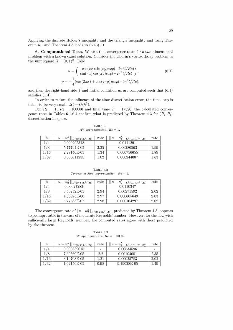
For Re = 1, Re = 100000 and final time T = 1/320, the calculated conver-gence rates in Tables 6.1-6.4 confirm what is predicted by Theorem 4.3 for (P2, P1)discretization in space.
Table 6.1AV approximation. Re = 1.
h ||u− uh1 ||L2(0,T ;L2(Ω)) rate ||u− uh
1 ||L2(0,T ;H1(Ω)) rate1/4 0.000295318 - 0.0111291 -1/8 5.77794E-05 2.35 0.00280563 1.991/16 2.28146E-05 1.34 0.000756655 1.891/32 0.000011235 1.02 0.000244007 1.63
Table 6.2Correction Step approximation. Re = 1.
h ||u− uh2 ||L2(0,T ;L2(Ω)) rate ||u− uh
2 ||L2(0,T ;H1(Ω)) rate1/4 0.00027283 - 0.0110347 -1/8 3.56252E-05 2.94 0.00271592 2.021/16 4.55025E-06 2.97 0.000665649 2.031/32 5.77583E-07 2.98 0.000164297 2.02
The convergence rate of ‖u−uh2‖L2(0,T ;L2(Ω)), predicted by Theorem 4.3, appears
to be improvable in the case of moderate Reynolds’ number. However, for the flow withsufficiently large Reynolds’ number, the computed rates agree with those predictedby the theorem.
Table 6.3AV approximation. Re = 100000.
h ||u− uh1 ||L2(0,T ;L2(Ω)) rate ||u− uh
1 ||L2(0,T ;H1(Ω)) rate1/4 0.000339015 - 0.00534596 -1/8 7.39569E-05 2.2 0.00104601 2.351/16 3.19763E-05 1.21 0.00025783 2.021/32 1.62156E-05 0.98 9.19028E-05 1.49
30
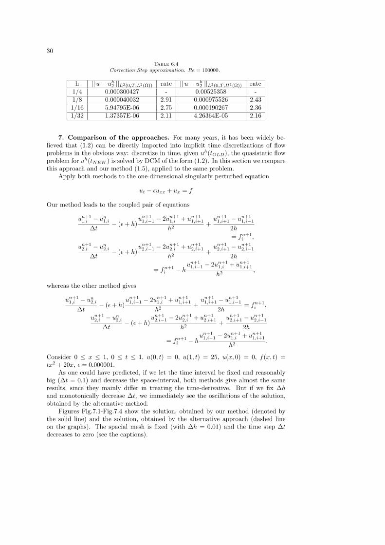
Table 6.4Correction Step approximation. Re = 100000.
h ||u− uh2 ||L2(0,T ;L2(Ω)) rate ||u− uh
2 ||L2(0,T ;H1(Ω)) rate1/4 0.000300427 - 0.00525358 -1/8 0.000040032 2.91 0.000975526 2.431/16 5.94795E-06 2.75 0.000190267 2.361/32 1.37357E-06 2.11 4.26364E-05 2.16
7. Comparison of the approaches. For many years, it has been widely be-lieved that (1.2) can be directly imported into implicit time discretizations of flowproblems in the obvious way: discretize in time, given uh(tOLD), the quasistatic flowproblem for uh(tNEW ) is solved by DCM of the form (1.2). In this section we comparethis approach and our method (1.5), applied to the same problem.
Apply both methods to the one-dimensional singularly perturbed equation
ut − εuxx + ux = f
Our method leads to the coupled pair of equations
un+11,i − un
1,i
∆t− (ε + h)
un+11,i−1 − 2un+1
1,i + un+11,i+1
h2+
un+11,i+1 − un+1
1,i−1
2h
= fn+1i ,
un+12,i − un
2,i
∆t− (ε + h)
un+12,i−1 − 2un+1
2,i + un+12,i+1
h2+
un+12,i+1 − un+1
2,i−1
2h
= fn+1i − h
un+11,i−1 − 2un+1
1,i + un+11,i+1
h2,
whereas the other method gives
un+11,i − un
2,i
∆t− (ε + h)
un+11,i−1 − 2un+1
1,i + un+11,i+1
h2+
un+11,i+1 − un+1
1,i−1
2h= fn+1
i ,
un+12,i − un
2,i
∆t− (ε + h)
un+12,i−1 − 2un+1
2,i + un+12,i+1
h2+
un+12,i+1 − un+1
2,i−1
2h
= fn+1i − h
un+11,i−1 − 2un+1
1,i + un+11,i+1
h2.
Consider 0 ≤ x ≤ 1, 0 ≤ t ≤ 1, u(0, t) = 0, u(1, t) = 25, u(x, 0) = 0, f(x, t) =tx2 + 20x, ε = 0.000001.
As one could have predicted, if we let the time interval be fixed and reasonablybig (∆t = 0.1) and decrease the space-interval, both methods give almost the sameresults, since they mainly differ in treating the time-derivative. But if we fix ∆hand monotonically decrease ∆t, we immediately see the oscillations of the solution,obtained by the alternative method.
Figures Fig.7.1-Fig.7.4 show the solution, obtained by our method (denoted bythe solid line) and the solution, obtained by the alternative approach (dashed lineon the graphs). The spacial mesh is fixed (with ∆h = 0.01) and the time step ∆tdecreases to zero (see the captions).
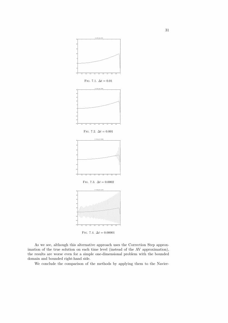
31
0 0.1 0.2 0.3 0.4 0.5 0.6 0.7 0.8 0.9 1−10
−5
0
5
10
15
20
25h = 0.01, ∆t = 0.01
Fig. 7.1. ∆t = 0.01
0 0.1 0.2 0.3 0.4 0.5 0.6 0.7 0.8 0.9 1−20
−15
−10
−5
0
5
10
15
20
25h = 0.01, ∆t = 0.001
Fig. 7.2. ∆t = 0.001
0 0.1 0.2 0.3 0.4 0.5 0.6 0.7 0.8 0.9 1−30
−20
−10
0
10
20
30
40h = 0.01, ∆t = 0.0002
Fig. 7.3. ∆t = 0.0002
0 0.1 0.2 0.3 0.4 0.5 0.6 0.7 0.8 0.9 1−30
−20
−10
0
10
20
30
40
50h = 0.01, ∆t = 1e−05
Fig. 7.4. ∆t = 0.00001
As we see, although this alternative approach uses the Correction Step approx-imation of the true solution on each time level (instead of the AV approximation),the results are worse even for a simple one-dimensional problem with the boundeddomain and bounded right-hand side.
We conclude the comparison of the methods by applying them to the Navier-
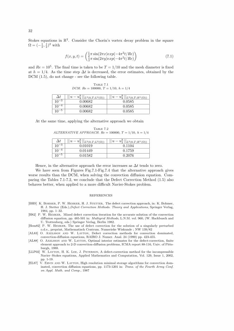
32
Stokes equations in R2. Consider the Chorin’s vortex decay problem in the squareΩ = (− 1
2 , 12 )2 with
f(x, y, t) =(
12π sin(2πx)exp(−4π2t/Re)12π sin(2πy)exp(−4π2t/Re)
)(7.1)
and Re = 105. The final time is taken to be T = 1/10 and the mesh diameter is fixedat h = 1/4. As the time step ∆t is decreased, the error estimates, obtained by theDCM (1.5), do not change - see the following table.
Table 7.1DCM. Re = 100000, T = 1/10, h = 1/4
∆t ||u− uh2 ||L2(0,T ;L2(Ω)) ||u− uh
2 ||L2(0,T ;H1(Ω))
10−3 0.00682 0.058510−4 0.00682 0.058510−5 0.00682 0.0585
At the same time, applying the alternative approach we obtain
Table 7.2ALTERNATIVE APPROACH. Re = 100000, T = 1/10, h = 1/4
∆t ||u− uh2 ||L2(0,T ;L2(Ω)) ||u− uh
2 ||L2(0,T ;H1(Ω))
10−3 0.01019 0.110410−4 0.01449 0.175910−5 0.01582 0.2076
Hence, in the alternative approach the error increases as ∆t tends to zero.We have seen from Figures Fig.7.1-Fig.7.4 that the alternative approach gives
worse results than the DCM, when solving the convection diffusion equation. Com-paring the Tables 7.1-7.2, we conclude that the Defect Correction Method (1.5) alsobehaves better, when applied to a more difficult Navier-Stokes problem.
REFERENCES
[BHS] K. Bohmer, P. W. Hemker, H. J. Stetter, The defect correction approach, in: K. Bohmer,H. J. Stetter (Eds.),Defect Correction Methods. Theory and Applications, Springer Verlag,1984, pp. 1–32.
[H82] P. W. Hemker, Mixed defect correction iteration for the accurate solution of the convectiondiffusion equation, pp. 485-501 in: Multigrid Methods, L.N.M. vol. 960, (W. Hackbusch andU. Trottenberg, eds.) Springer Verlag, Berlin 1982.
[Hem82] P. W. Hemker, The use of defect correction for the solution of a singularly perturbedo.d.e., preprint, Mathematisch Centrum. Numerieke Wiskunde ; NW 139/82
[AL83] O. Axelsson and W. Layton, Defect correction methods for convection dominated,convection-diffusion equations, RAIRO J. Numer. Anal. 24 (1990) pp. 423-455.
[AL88] O. Axelsson and W. Layton, Optimal interior estimates for the defect-correction, finiteelement approach to 2-D convection-diffusion problems, ICMA report 88-116, Univ. of Pitts-burgh, 1988.
[LLP02] W. Layton, H. K. Lee, J. Peterson, A defect-correction method for the incompressibleNavier–Stokes equations, Applied Mathematics and Computation, Vol. 129, Issue 1, 2002,pp. 1-19.
[EL87] V. Ervin and W. Layton, High resolution minimal storage algorithms for convection dom-inated, convection diffusion equations, pp. 1173-1201 in: Trans. of the Fourth Army Conf.on Appl. Math. and Comp., 1987

33
[EL89] V. Ervin and W. Layton, An analysis of a defect correction method for a model convectiondiffusion equation, SIAM J. Numer. Anal., 26 (1989), 169-179.
[ELM00] V. Ervin, W. Layton, J. Maubach, Adaptive defect correction methods for viscous in-compressible flow problems, SIAM J. Numer. Anal., 37 (2000), pp. 1165-1185.
[Hei96] W. Heinrichs, Defect correction for convection dominated flow, SIAM J. Sci. Comput., 17(1996), 1082-1091
[H82-1] P. Hemker, An accurate method without directional bias for the numerical solution of a2-D elliptic singular perturbation problem, pp. 192-206 in: Theory And Applications OfSingular Perturbations, Lecture Notes in Math. 942, W. Eckhaus and E.M. de Jaeger, eds.,Sprienger-Verlag, Berlin, 1982
[L2007] W. Layton, Introduction to the Numerical Analysis of Incompressible, Viscous Flow, toappear in 2007.
[HR90] J. Heywood, R. Rannacher, Finite-element approximations of the nonstationary Navier-Stokes problem. Part 4: Error analysis for second-order time discretization, SIAM J. Numer.Anal., 2 (1990)
[K91] B. Koren, Multigrid and Defect-Correction for the Steady Navier-Stokes Equations, Ap-plications to Aerodynamics, C. W. I. Tract 74, Centrum voor Wiskunde en Informatica,Amsterdam, 1991.
[LK93] M.-H. Lallemand, B. Koren, Iterative defect correction and multigrid accelerated explicittime stepping schemes for the steady Euler equations, SIAM Journal on Scientific Comput-ing, vol. 14, issue 4, 1993.
[EL06] V. J. Ervin, H. K. Lee, Defect correction method for viscoelastic fluid flows at high Weis-senberg number, Numerical Methods for Partial Differential Equations, Volume 22, Issue 1,pp. 145 - 164, 2006.
[HSS] P. W. Hemker, G. I. Shishkin, L. P. Shishkina, High-order time-accurate schemes for sin-gularly perturbed parabolic convection-diffusion problems with Robin boundary conditions,Computational Methods in Applied Mathematics, Vol. 2 (2002), No. 1, pp. 3-25.
[GR79] V. Girault, P.A. Raviart, Finite element approximation of the Navier-Stokes equations,Lecture notes in mathematics, no. 749, Springer-Verlag, 1979.
[MF04] J. H. Mathews, K. D. Fink, Numerical Analysis - Numerical Methods, 2004.[M04] M. L. Minion, Semi-Implicit Projection Methods for Incompressible Flow based on Spectral
Deferred Corrections, Appl. Numer. Math., 48(3-4), 369-387, 2004[BLM03] A. Bourlioux, A. T. Layton, M. L. Minion, High-Order Multi-Implicit Spectral
Deferred Correction Methods for Problems of Reactive Flows, Journal of ComputationalPhysics, Vol. 189, No. 2, pp. 651-675, 2003.
[KG02] W. Kress, B. Gustafsson, Deferred Correction Methods for Initial Boundary Value Prob-lems, Journal of Scientific Computing, Springer Netherlands, Vol. 17, No. 1-4, 2002.
[DGR00] A. Dutt, L. Greengard, V. Rokhlin, Spectral deferred correction methods for ordinarydifferential equations, BIT 40 (2), pp. 241-266, 2000.