Embed Size (px)
Citation preview
POLİTEKNİK DERGİSİ JOURNAL of POLYTECHNIC ISSN: 1302-0900 (PRINT), ISSN: 2147-9429 (ONLINE)
URL: http://dergipark.gov.tr/politeknik
A data mining application of local weather
forecast for Kayseri Erkilet Airport
Yazar(lar) (Author(s)): Eda ÇINAROĞLU1, Osman UNUTULMAZ
ORCID1: 0000-0002-2904-3376
Bu makaleye şu şekilde atıfta bulunabilirsiniz (To cite to this article) : Çınaroğlu E. ve Unutulmaz O.,
“A data mining application of local weather forecast for Kayseri Erkilet Airport”, Politeknik Dergisi, 22(1):
103-113, (2019).
Erişim linki (To link to this article): http://dergipark.gov.tr/politeknik/archive
DOI: 10.2339/politeknik.391801
DOI:
Politeknik Dergisi, 2019; 22(1) : 103-113 Journal of Polytechnic, 2019; 22 (1) : 103-113
103
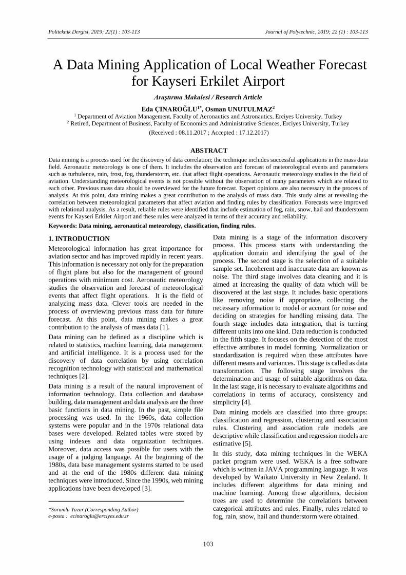
A Data Mining Application of Local Weather Forecast
for Kayseri Erkilet Airport Araştırma Makalesi / Research Article
Eda ÇINAROĞLU1*, Osman UNUTULMAZ2
1 Department of Aviation Management, Faculty of Aeronautics and Astronautics, Erciyes University, Turkey 2 Retired, Department of Business, Faculty of Economics and Administrative Sciences, Erciyes University, Turkey
(Received : 08.11.2017 ; Accepted : 17.12.2017)
ABSTRACT
Data mining is a process used for the discovery of data correlation; the technique includes successful applications in the mass data
field. Aeronautic meteorology is one of them. It includes the observation and forecast of meteorological events and parameters
such as turbulence, rain, frost, fog, thunderstorm, etc. that affect flight operations. Aeronautic meteorology studies in the field of
aviation. Understanding meteorological events is not possible without the observation of many parameters which are related to
each other. Previous mass data should be overviewed for the future forecast. Expert opinions are also necessary in the process of
analysis. At this point, data mining makes a great contribution to the analysis of mass data. This study aims at revealing the
correlation between meteorological parameters that affect aviation and finding rules by classification. Forecasts were improved
with relational analysis. As a result, reliable rules were identified that include estimation of fog, rain, snow, hail and thunderstorm
events for Kayseri Erkilet Airport and these rules were analyzed in terms of their accuracy and reliability.
Keywords: Data mining, aeronautical meteorology, classification, finding rules.
1. INTRODUCTION
Meteorological information has great importance for
aviation sector and has improved rapidly in recent years.
This information is necessary not only for the preparation
of flight plans but also for the management of ground
operations with minimum cost. Aeronautic meteorology
studies the observation and forecast of meteorological
events that affect flight operations. It is the field of
analyzing mass data. Clever tools are needed in the
process of overviewing previous mass data for future
forecast. At this point, data mining makes a great
contribution to the analysis of mass data [1].
Data mining can be defined as a discipline which is
related to statistics, machine learning, data management
and artificial intelligence. It is a process used for the
discovery of data correlation by using correlation
recognition technology with statistical and mathematical
techniques [2].
Data mining is a result of the natural improvement of
information technology. Data collection and database
building, data management and data analysis are the three
basic functions in data mining. In the past, simple file
processing was used. In the 1960s, data collection
systems were popular and in the 1970s relational data
bases were developed. Related tables were stored by
using indexes and data organization techniques.
Moreover, data access was possible for users with the
usage of a judging language. At the beginning of the
1980s, data base management systems started to be used
and at the end of the 1980s different data mining
techniques were introduced. Since the 1990s, web mining
applications have been developed [3].
Data mining is a stage of the information discovery
process. This process starts with understanding the
application domain and identifying the goal of the
process. The second stage is the selection of a suitable
sample set. Incoherent and inaccurate data are known as
noise. The third stage involves data cleaning and it is
aimed at increasing the quality of data which will be
discovered at the last stage. It includes basic operations
like removing noise if appropriate, collecting the
necessary information to model or account for noise and
deciding on strategies for handling missing data. The
fourth stage includes data integration, that is turning
different units into one kind. Data reduction is conducted
in the fifth stage. It focuses on the detection of the most
effective attributes in model forming. Normalization or
standardization is required when these attributes have
different means and variances. This stage is called as data
transformation. The following stage involves the
determination and usage of suitable algorithms on data.
In the last stage, it is necessary to evaluate algorithms and
correlations in terms of accuracy, consistency and
simplicity [4].
Data mining models are classified into three groups:
classification and regression, clustering and association
rules. Clustering and association rule models are
descriptive while classification and regression models are
estimative [5].
In this study, data mining techniques in the WEKA
packet program were used. WEKA is a free software
which is written in JAVA programming language. It was
developed by Waikato University in New Zealand. It
includes different algorithms for data mining and
machine learning. Among these algorithms, decision
trees are used to determine the correlations between
categorical attributes and rules. Finally, rules related to
fog, rain, snow, hail and thunderstorm were obtained. *Sorumlu Yazar (Corresponding Author)
e-posta : [email protected]

Eda ÇINAROĞLU, Osman UNUTULMAZ /POLİTEKNİK DERGİSİ, Politeknik Dergisi,2019;22(1):103-113
104
A number of researchers focused on techniques for the
determination of meteorological parameters for a long
time. There are many studies on this subject in the
literature. These studies include the usage of artificial
neural networks, genetic algorithms, decision trees and
regression for the analysis and forecast of parameters.
Some of these studies may be summarized as follows.
Allen and LeMarshall (1994) revealed the successful
usage of neural networks for rainfall forecast. They built
a model on the basis of 665 days’ data. This model, which
can estimate the potential for rain in a 24 hour period,
could only reach a 70% accuracy rate [6].
McGullag and colleagues (1997) conducted a study
which reflects the fact that the neural network is a good
method for similar problems. They preferred to use the
genetic reduction method to decrease the number of input
parameters from 62 to 18. The result of this classification
method is that there is rain or there is no rain. The
accuracy rate of this model is higher than that achieved
by the model developed by Allen and LeMarshall (1994)
[7].
Stern and Parkyn (1999) studied fog estimation for
Melbourne Airport to determine visibility. In this
research, with two objectives in mind, the logistic
regression method was employed. The first objective was
to develop a classification rule for foggy conditions by
using synoptic data; the second was to develop a
technique which estimates the probability of fog in a
specific period of time [8].
Mitsukura, Fukumi and Akamatsu (2000) conducted
research about fog estimation. They used the Learning
Vector Quantization (LVQ) method in their study and
input parameters were selected by the genetic algorithm
to increase the reliability of the study [9].
Trafalis and colleagues (2002) used data mining for
rainfall estimation. They developed a neural network
model using the data that they obtained from Oklahoma
Mesonet [10].
Solomantine and Dulal (2003) investigated model trees
for rainfall estimation. Model trees are very similar to
decision trees. The significant difference between
decision and model trees is that there are regression
functions on the leaves of model trees whereas there are
classification labels on the leaves of decision trees [11].
According to Lee and Liu (2004), fuzzy logic is suitable
for meteorological estimation. The attributes of their
rainfall forecast model are temperature, dew temperature,
humidity, wind speed, wind direction and average sea
level pressure [12].
Jareanpon and his colleagues (2004) used the radial basis
neural network and genetic algorithms together for
rainfall estimation in their study. Thirty years monthly
rainfall values dating between 1971 and 2000, which
were obtained from the Thailand Meteorology Office
were used [13].
Suvichakorn and Tatnall (2005) conducted research on
rainfall estimation by using cloud structure and
movement. They used the k-nearest neighbor algorithm
based on supervised learning in their study [14].
Banik and colleagues (2008) state that the neural network
and genetic algorithm methods are more useful than
multi-linear regression models for Bangladesh’s
monsoon rainfall estimation because of the dynamic,
multi-dimension and nonlinear functions of precipitation
data [15].
Pan and Wu (2009) developed a model which includes
the Bayes technique and neural networks for rainfall
estimation. Like earlier studies, they used pressure,
temperature, wind speed and direction as input
parameters [16].
Moreover, in another study conducted by Aktaş and
Erkuş (2009), the researchers preferred to use logistics
regression analysis for Eskişehir fog estimation. The
research aimed at finding the equation showing the
possibility of fog event occurring [17].
Bartok and colleagues (2010) state in their research that
data mining applications are successful at fog and cloud
base estimation. They used synoptic and metar
observations along with air satellite images in their
model. They also emphasized that the information
obtained would be useful for airports and traffic services
[18].
Zazzaro and Mercogliano (2010) developed a new
classification algorithm for rarely seen meteorological
events. Fog forecast data were evaluated by a new
algorithm based on Bayes Network. The study aimed at
minimum incorrect classification cost [19].
Wu (2011) emphasized the fact that rainfall problems
involved complicated system dynamics because of the
linear and nonlinear meteorological factor effects. As a
result, he developed a semi-parametric and hybrid
regression model with a high accuracy rate [20].
Lee and Seo (2013) used a multiple linear regression
method to build a statistical forecasting model for
Changma, the Korean portion of the East Asia summer
monsoon system. The predictors in the model were
selected by a forward-stepwise regression method using
three criteria that minimized overfitting. The prediction
skill of the model for the years 1994–2012 was very high
with the correlation coefficient R=0.85 [21].
In this study, the first section includes information about
data mining and different meteorological applications in
the literature. In the second section problem definition,
methods, results and rules’ assessment are presented. The
conclusion and discussion are found in the last section.
2. DATA MINING APPLICATION
2.1. Problem Definition
The aim of this study is to develop rules that can be used
for the local forecast of fog, precipitation and
thunderstorm events at Kayseri Erkilet Airport. These
rules were developed by using data mining classification
methods.
A DATA MINING APPLICATION OF LOCAL WEATER FORECAST FOR KAYSERİ ERKI… Politeknik Dergisi, 2019; 22 (1) : 103-113
105
2.2. Data Set
The data set includes 15330 days’ values collected from
1970-2012. The measurements were taken twice a day at
2 am and 2 pm. The 2 am measurements were preferred
since night measurements are more reliable and robust.
The data were taken from the TUMAS archive system. It
was formed from observations, measurements and
calculations by the Head Office of the Turkish
Meteorological Department. The free observation values
issued by Wyoming University Atmosphere Science
Department were also included in the project.
Metar, rawinsonde and climate observations were used in
this research. Metar observations, which are measured by
the meteorology department of airports, include ground
values. Rawinsonde observations are high level values
acquired by using balloons. Climate observations show
ground values like metar observations and they are used
for climate studies.
Climate observations include pressure, min-max
temperature difference, cloudiness, temperature, relative
humidity, vapor pressure, wind speed, the amount of
vaporization, rainfall, sun exposure and its duration.
The rawinsonde observations for Kayseri were needed
while climate and metar observations were taken from
the database. Rawinsonde observations are measured in
eight centers in Turkey. The values of the surrounding
cities of Samsun, Ankara, Adana, Diyarbakır and
Erzurum were used to estimate Kayseri values, which
have regional variation. At this point, nearest
neighborhood, surface trend analysis and inverse
distance weighting methods were tested on the data. It
was tried to detect the method with minimum error,
regarding one of the city’s values are not known at every
turn and obtaining estimation for this city. The inverse
distance weighting method was found as the most
suitable for the data structure. The interpolation weights
of neighboring cities were found as follows:
Samsun: 20%
Ankara: 24%
Adana: 30%
Diyarbakır: 14%
Erzurum: 12%
Rawinsonde observations include meteorological
information recorded at different atmospheric pressures,
in other words, at different height levels. Such basic
levels as 1000 mb, 850 mb, 700 mb, 500 mb, 400 mb,
300 mb, 200 mb and 100 mb are included in the database.
The data between 1000 mb-300 mb levels were used in
this study since 1000 mb-300 mb is the flying zone and
no meteorological events occur above 20000 feet.
The data of different height levels are named as follows:
PRES: Atmospheric pressure (HPa)
HGHT: Height (mt)
TEMP: Temperature (0C)
DWPT: Dew temperature (0C)
RELH: Relative humidity (%)
MIXR: Mix ratio (gr/kg)
DRCT: Wind direction (degree)
SKNT: Wind speed (knot)
THTA: Potential temperature (Kelvin)
THTE: Equivalent potential temperature (Kelvin)
THTV: Virtual potential temperature (Kelvin)
Some meteorological parameters and indexes are used in
the study while forming the rules for precipitation and
thunderstorm. The explanations of these values are given
as follows:
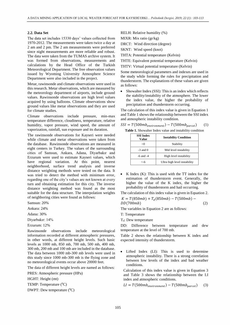
Showalter Index (SSI): This is an index which reflects
the stability/instability of the atmosphere. The lower
the index value, the higher the probability of
precipitation and thunderstorm occurring.
The calculation of this index value is given in Equation 1
and Table 1 shows the relationship between the SSI index
and atmospheric instability condition.
𝑆𝑆𝐼 = 𝑇(500𝑚𝑏𝑒𝑛𝑣𝑖𝑟𝑜𝑛𝑚𝑒𝑛𝑡) − 𝑇(500𝑚𝑏𝑝𝑎𝑟𝑐𝑒𝑙) (1)
Table 1. Showalter Index value and instability condition
SSI Index
Value Instability Condition
>0 Stability
-3 and 0 Mid level instability
-6 and -4 High level instability
<-6 Ultra high level instability
K Index (K): This is used with the TT index for the
estimation of thunderstorm event. Generally, the
higher the value of the K index, the higher the
probability of thunderstorm and hail occurring.
The calculation of this index value is given in Equation 2.
𝐾 = 𝑇(850𝑚𝑏) + 𝑇𝑑(850𝑚𝑏) − 𝑇(500𝑚𝑏) −𝐷𝐷(700𝑚𝑏) (2)
The variables in Equation 2 are as follows:
T: Temperature
Td: Dew temperature
DD: Difference between temperature and dew
temperature at the level of 700 mb.
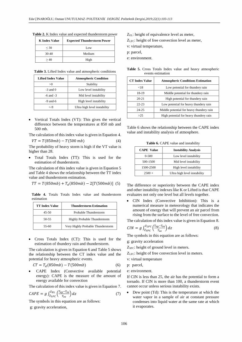
Table 2 shows the relationship between K index and
expected intensity of thunderstorm.
Lifted Index (LI): This is used to determine
atmospheric instability. There is a strong correlation
between low levels of the index and bad weather
conditions.
Calculation of this index value is given in Equation 3
and Table 3 shows the relationship between the LI
index and atmospheric conditions.
𝐿𝐼 = 𝑇(500𝑚𝑏𝑒𝑛𝑣𝑖𝑟𝑜𝑛𝑚𝑒𝑛𝑡) − 𝑇(500𝑚𝑏𝑝𝑎𝑟𝑐𝑒𝑙) (3)
Eda ÇINAROĞLU, Osman UNUTULMAZ /POLİTEKNİK DERGİSİ, Politeknik Dergisi,2019;22(1):103-113
106
Table 2. K Index value and expected thunderstorm power
K Index Value Expected Thunderstorm Power
≤ 30 Low
30-40 Medium
≥ 40 High
Table 3. Lifted Index value and atmospheric conditions
Lifted Index Value Atmospheric Condition
>0 Stability
-3 and 0 Low level instability
-6 and -3 Mid level instability
-9 and-6 High level instability
<-9 Ultra high level instability
Vertical Totals Index (VT): This gives the vertical
difference between the temperatures at 850 mb and
500 mb.
The calculation of this index value is given in Equation 4.
𝑉𝑇 = 𝑇(850𝑚𝑏) − 𝑇(500 𝑚𝑏) (4)
The probability of heavy storm is high if the VT value is
higher than 28.
Total Totals Index (TT): This is used for the
estimation of thunderstorm.
The calculation of this index value is given in Equation 5
and Table 4 shows the relationship between the TT index
value and thunderstorm estimation.
𝑇𝑇 = 𝑇(850𝑚𝑏) + 𝑇𝑑(850𝑚𝑏) − 2[𝑇(500𝑚𝑏)] (5)
Table 4. Totals Totals Index value and thunderstorm
estimation
TT Index Value Thunderstorm Estimation
45-50 Probable Thunderstorm
50-55 Highly Probable Thunderstorm
55-60 Very Highly Probable Thunderstorm
Cross Totals Index (CT): This is used for the
estimation of thundery rain and thunderstorm.
The calculation is given in Equation 6 and Table 5 shows
the relationship between the CT index value and the
potential for heavy atmospheric events.
𝐶𝑇 = 𝑇𝑑(850𝑚𝑏) − 𝑇(500𝑚𝑏) (6)
CAPE Index (Convective available potential
energy): CAPE is the measure of the amount of
energy available for convection
The calculation of this index value is given in Equation 7.
𝐶𝐴𝑃𝐸 = 𝑔 ∫ (𝑇𝑣𝑝−𝑇𝑣𝑒
𝑇𝑣𝑒) 𝑑𝑧
𝑍𝐸𝐿
𝑍𝐿𝐹𝐶 (7)
The symbols in this equation are as follows:
g: gravity acceleration,
ZEL: height of equivalence level as meter,
ZLFC: height of free convection level as meter,
v: virtual temperature,
p: parcel,
e: environment.
Table 5. Cross Totals Index value and heavy atmospheric
events estimation
CT Index Value Atmospheric Conditions Estimation
<18 Low potential for thundery rain
18-19 Middle potential for thundery rain
20-21 High potential for thundery rain
22-23 Low potential for heavy thundery rain
24-25 Middle potential for heavy thundery rain
>25 High potential for heavy thundery rain
Table 6 shows the relationship between the CAPE index
value and instability analysis of atmosphere.
Table 6. CAPE value and instability
CAPE Value Instability Analysis
0-500 Low level instability
500-1500 Mid level instability
1500-2500 High level instability
2500 + Ultra high level instability
The difference or superiority between the CAPE index
and other instability indexes like K or Lifted is that CAPE
evaluates not only one level but all levels together.
CIN Index (Convective Inhibition): This is a
numerical measure in meteorology that indicates the
amount of energy that will prevent an air parcel from
rising from the surface to the level of free convection.
The calculation of this index value is given in Equation 8.
𝐶𝐼𝑁 = 𝑔 ∫ (𝑇𝑣𝑝−𝑇𝑣𝑒
𝑇𝑣𝑒) 𝑑𝑧
𝑍𝐿𝐹𝐶
𝑍𝑆𝐹𝐶 (8)
The symbols in this equation are as follows:
g: gravity acceleration
ZSFC: height of ground level in meters.
ZLFC: height of free convection level in meters.
v: virtual temperature
p: parcel,
e: environment.
If CIN is less than 25, the air has the potential to form a
tornado. If CIN is more than 100, a thunderstorm event
cannot occur unless serious instability exists.
Dew point (Td): This is the temperature at which the
water vapor in a sample of air at constant pressure
condenses into liquid water at the same rate at which
it evaporates.
A DATA MINING APPLICATION OF LOCAL WEATER FORECAST FOR KAYSERİ ERKI… Politeknik Dergisi, 2019; 22 (1) : 103-113
107
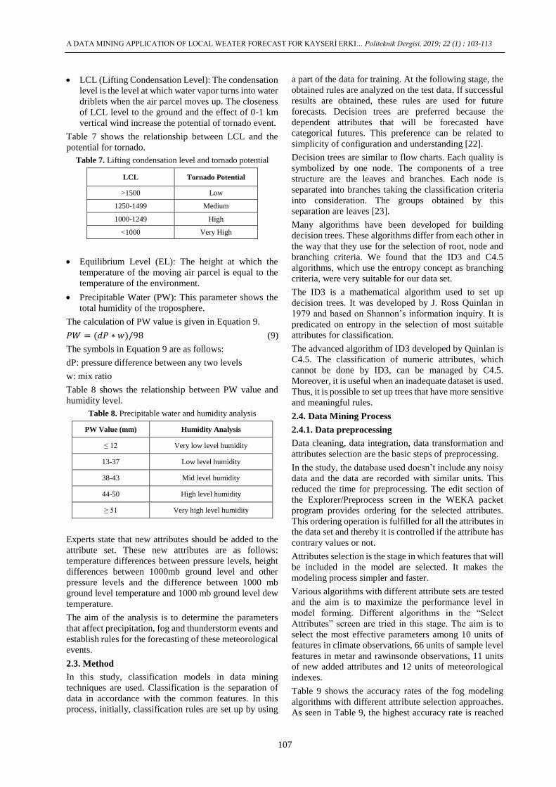
LCL (Lifting Condensation Level): The condensation
level is the level at which water vapor turns into water
driblets when the air parcel moves up. The closeness
of LCL level to the ground and the effect of 0-1 km
vertical wind increase the potential of tornado event.
Table 7 shows the relationship between LCL and the
potential for tornado.
Table 7. Lifting condensation level and tornado potential
LCL Tornado Potential
>1500 Low
1250-1499 Medium
1000-1249 High
<1000 Very High
Equilibrium Level (EL): The height at which the
temperature of the moving air parcel is equal to the
temperature of the environment.
Precipitable Water (PW): This parameter shows the
total humidity of the troposphere.
The calculation of PW value is given in Equation 9.
𝑃𝑊 = (𝑑𝑃 ∗ 𝑤)/98 (9)
The symbols in Equation 9 are as follows:
dP: pressure difference between any two levels
w: mix ratio
Table 8 shows the relationship between PW value and
humidity level.
Table 8. Precipitable water and humidity analysis
PW Value (mm) Humidity Analysis
≤ 12 Very low level humidity
13-37 Low level humidity
38-43 Mid level humidity
44-50 High level humidity
≥ 51 Very high level humidity
Experts state that new attributes should be added to the
attribute set. These new attributes are as follows:
temperature differences between pressure levels, height
differences between 1000mb ground level and other
pressure levels and the difference between 1000 mb
ground level temperature and 1000 mb ground level dew
temperature.
The aim of the analysis is to determine the parameters
that affect precipitation, fog and thunderstorm events and
establish rules for the forecasting of these meteorological
events.
2.3. Method
In this study, classification models in data mining
techniques are used. Classification is the separation of
data in accordance with the common features. In this
process, initially, classification rules are set up by using
a part of the data for training. At the following stage, the
obtained rules are analyzed on the test data. If successful
results are obtained, these rules are used for future
forecasts. Decision trees are preferred because the
dependent attributes that will be forecasted have
categorical futures. This preference can be related to
simplicity of configuration and understanding [22].
Decision trees are similar to flow charts. Each quality is
symbolized by one node. The components of a tree
structure are the leaves and branches. Each node is
separated into branches taking the classification criteria
into consideration. The groups obtained by this
separation are leaves [23].
Many algorithms have been developed for building
decision trees. These algorithms differ from each other in
the way that they use for the selection of root, node and
branching criteria. We found that the ID3 and C4.5
algorithms, which use the entropy concept as branching
criteria, were very suitable for our data set.
The ID3 is a mathematical algorithm used to set up
decision trees. It was developed by J. Ross Quinlan in
1979 and based on Shannon’s information inquiry. It is
predicated on entropy in the selection of most suitable
attributes for classification.
The advanced algorithm of ID3 developed by Quinlan is
C4.5. The classification of numeric attributes, which
cannot be done by ID3, can be managed by C4.5.
Moreover, it is useful when an inadequate dataset is used.
Thus, it is possible to set up trees that have more sensitive
and meaningful rules.
2.4. Data Mining Process
2.4.1. Data preprocessing
Data cleaning, data integration, data transformation and
attributes selection are the basic steps of preprocessing.
In the study, the database used doesn’t include any noisy
data and the data are recorded with similar units. This
reduced the time for preprocessing. The edit section of
the Explorer/Preprocess screen in the WEKA packet
program provides ordering for the selected attributes.
This ordering operation is fulfilled for all the attributes in
the data set and thereby it is controlled if the attribute has
contrary values or not.
Attributes selection is the stage in which features that will
be included in the model are selected. It makes the
modeling process simpler and faster.
Various algorithms with different attribute sets are tested
and the aim is to maximize the performance level in
model forming. Different algorithms in the “Select
Attributes” screen are tried in this stage. The aim is to
select the most effective parameters among 10 units of
features in climate observations, 66 units of sample level
features in metar and rawinsonde observations, 11 units
of new added attributes and 12 units of meteorological
indexes.
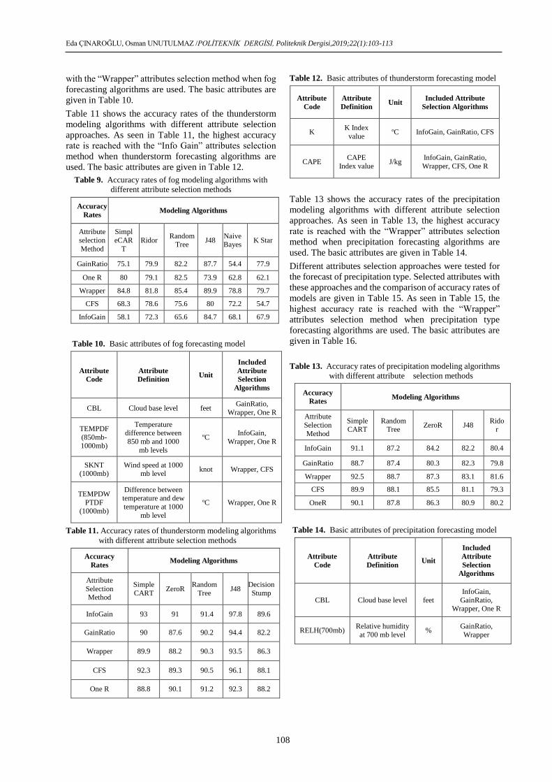
Table 9 shows the accuracy rates of the fog modeling
algorithms with different attribute selection approaches.
As seen in Table 9, the highest accuracy rate is reached
Eda ÇINAROĞLU, Osman UNUTULMAZ /POLİTEKNİK DERGİSİ, Politeknik Dergisi,2019;22(1):103-113
108
with the “Wrapper” attributes selection method when fog
forecasting algorithms are used. The basic attributes are
given in Table 10.
Table 11 shows the accuracy rates of the thunderstorm
modeling algorithms with different attribute selection
approaches. As seen in Table 11, the highest accuracy
rate is reached with the “Info Gain” attributes selection
method when thunderstorm forecasting algorithms are
used. The basic attributes are given in Table 12.
Table 9. Accuracy rates of fog modeling algorithms with
different attribute selection methods
Accuracy
Rates Modeling Algorithms
Attribute
selection
Method
Simpl
eCAR
T
Ridor Random
Tree J48
NaiveBayes
K Star
GainRatio 75.1 79.9 82.2 87.7 54.4 77.9
One R 80 79.1 82.5 73.9 62.8 62.1
Wrapper 84.8 81.8 85.4 89.9 78.8 79.7
CFS 68.3 78.6 75.6 80 72.2 54.7
InfoGain 58.1 72.3 65.6 84.7 68.1 67.9
Table 10. Basic attributes of fog forecasting model
Attribute
Code
Attribute
Definition Unit
Included
Attribute
Selection
Algorithms
CBL Cloud base level feet GainRatio,
Wrapper, One R
TEMPDF
(850mb-1000mb)
Temperature
difference between
850 mb and 1000
mb levels
oC InfoGain,
Wrapper, One R
SKNT (1000mb)
Wind speed at 1000 mb level
knot Wrapper, CFS
TEMPDW
PTDF (1000mb)
Difference between temperature and dew
temperature at 1000
mb level
oC Wrapper, One R
Table 11. Accuracy rates of thunderstorm modeling algorithms
with different attribute selection methods
Accuracy
Rates Modeling Algorithms
Attribute
Selection Method
Simple
CART ZeroR
Random
Tree J48
Decision
Stump
InfoGain 93 91 91.4 97.8 89.6
GainRatio 90 87.6 90.2 94.4 82.2
Wrapper 89.9 88.2 90.3 93.5 86.3
CFS 92.3 89.3 90.5 96.1 88.1
One R 88.8 90.1 91.2 92.3 88.2
Table 12. Basic attributes of thunderstorm forecasting model
Attribute
Code
Attribute
Definition Unit
Included Attribute
Selection Algorithms
K K Index
value oC InfoGain, GainRatio, CFS
CAPE CAPE
Index value J/kg
InfoGain, GainRatio,
Wrapper, CFS, One R
Table 13 shows the accuracy rates of the precipitation
modeling algorithms with different attribute selection
approaches. As seen in Table 13, the highest accuracy
rate is reached with the “Wrapper” attributes selection
method when precipitation forecasting algorithms are
used. The basic attributes are given in Table 14.
Different attributes selection approaches were tested for
the forecast of precipitation type. Selected attributes with
these approaches and the comparison of accuracy rates of
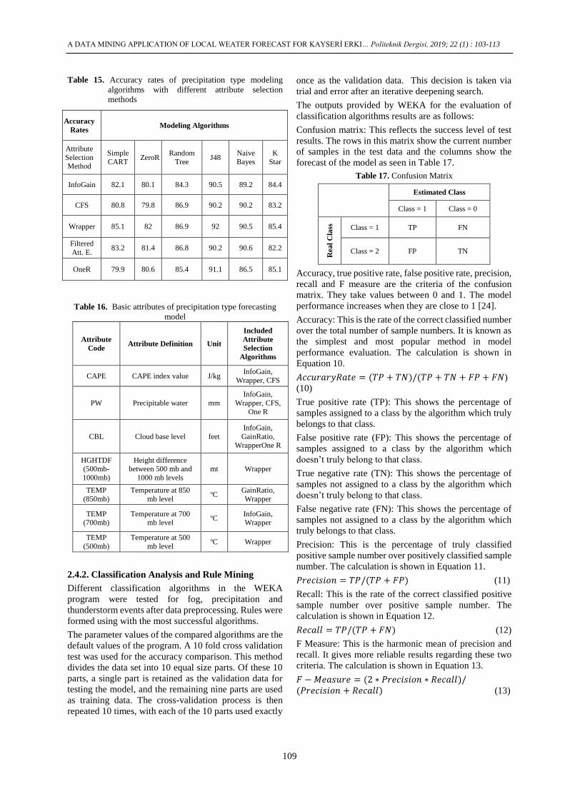
models are given in Table 15. As seen in Table 15, the
highest accuracy rate is reached with the “Wrapper”
attributes selection method when precipitation type
forecasting algorithms are used. The basic attributes are
given in Table 16.
Table 13. Accuracy rates of precipitation modeling algorithms
with different attribute selection methods
Accuracy
Rates Modeling Algorithms
Attribute
Selection
Method
Simple
CART
Random
Tree ZeroR J48
Rido
r
InfoGain 91.1 87.2 84.2 82.2 80.4
GainRatio 88.7 87.4 80.3 82.3 79.8
Wrapper 92.5 88.7 87.3 83.1 81.6
CFS 89.9 88.1 85.5 81.1 79.3
OneR 90.1 87.8 86.3 80.9 80.2
Table 14. Basic attributes of precipitation forecasting model
Attribute
Code
Attribute
Definition Unit
Included
Attribute
Selection
Algorithms
CBL Cloud base level feet
InfoGain,
GainRatio,
Wrapper, One R
RELH(700mb) Relative humidity
at 700 mb level %
GainRatio,
Wrapper
A DATA MINING APPLICATION OF LOCAL WEATER FORECAST FOR KAYSERİ ERKI… Politeknik Dergisi, 2019; 22 (1) : 103-113
109
Table 15. Accuracy rates of precipitation type modeling
algorithms with different attribute selection
methods
Accuracy
Rates Modeling Algorithms
Attribute
Selection Method
Simple
CART ZeroR
Random
Tree J48
Naive
Bayes
K
Star
InfoGain 82.1 80.1 84.3 90.5 89.2 84.4
CFS 80.8 79.8 86.9 90.2 90.2 83.2
Wrapper 85.1 82 86.9 92 90.5 85.4
Filtered
Att. E. 83.2 81.4 86.8 90.2 90.6 82.2
OneR 79.9 80.6 85.4 91.1 86.5 85.1
Table 16. Basic attributes of precipitation type forecasting
model
Attribute
Code Attribute Definition Unit
Included
Attribute
Selection
Algorithms
CAPE CAPE index value J/kg InfoGain,
Wrapper, CFS
PW Precipitable water mm
InfoGain,
Wrapper, CFS,
One R
CBL Cloud base level feet
InfoGain,
GainRatio,
WrapperOne R
HGHTDF (500mb-
1000mb)
Height difference between 500 mb and
1000 mb levels
mt Wrapper
TEMP
(850mb)
Temperature at 850
mb level oC
GainRatio,
Wrapper
TEMP (700mb)
Temperature at 700 mb level
oC InfoGain, Wrapper
TEMP
(500mb)
Temperature at 500
mb level oC Wrapper
2.4.2. Classification Analysis and Rule Mining
Different classification algorithms in the WEKA
program were tested for fog, precipitation and
thunderstorm events after data preprocessing. Rules were
formed using with the most successful algorithms.
The parameter values of the compared algorithms are the
default values of the program. A 10 fold cross validation
test was used for the accuracy comparison. This method
divides the data set into 10 equal size parts. Of these 10
parts, a single part is retained as the validation data for
testing the model, and the remaining nine parts are used
as training data. The cross-validation process is then
repeated 10 times, with each of the 10 parts used exactly
once as the validation data. This decision is taken via
trial and error after an iterative deepening search.
The outputs provided by WEKA for the evaluation of
classification algorithms results are as follows:
Confusion matrix: This reflects the success level of test
results. The rows in this matrix show the current number
of samples in the test data and the columns show the
forecast of the model as seen in Table 17.
Table 17. Confusion Matrix
Estimated Class
Class = 1 Class = 0
Rea
l C
lass
Class = 1 TP FN
Class = 2 FP TN
Accuracy, true positive rate, false positive rate, precision,
recall and F measure are the criteria of the confusion
matrix. They take values between 0 and 1. The model
performance increases when they are close to 1 [24].
Accuracy: This is the rate of the correct classified number
over the total number of sample numbers. It is known as
the simplest and most popular method in model
performance evaluation. The calculation is shown in
Equation 10.
𝐴𝑐𝑐𝑢𝑟𝑎𝑟𝑦𝑅𝑎𝑡𝑒 = (𝑇𝑃 + 𝑇𝑁)/(𝑇𝑃 + 𝑇𝑁 + 𝐹𝑃 + 𝐹𝑁)
(10)
True positive rate (TP): This shows the percentage of
samples assigned to a class by the algorithm which truly
belongs to that class.
False positive rate (FP): This shows the percentage of
samples assigned to a class by the algorithm which
doesn’t truly belong to that class.
True negative rate (TN): This shows the percentage of
samples not assigned to a class by the algorithm which
doesn’t truly belong to that class.
False negative rate (FN): This shows the percentage of
samples not assigned to a class by the algorithm which
truly belongs to that class.
Precision: This is the percentage of truly classified
positive sample number over positively classified sample
number. The calculation is shown in Equation 11.
𝑃𝑟𝑒𝑐𝑖𝑠𝑖𝑜𝑛 = 𝑇𝑃/(𝑇𝑃 + 𝐹𝑃) (11)
Recall: This is the rate of the correct classified positive
sample number over positive sample number. The
calculation is shown in Equation 12.
𝑅𝑒𝑐𝑎𝑙𝑙 = 𝑇𝑃/(𝑇𝑃 + 𝐹𝑁) (12)
F Measure: This is the harmonic mean of precision and
recall. It gives more reliable results regarding these two
criteria. The calculation is shown in Equation 13.
𝐹 − 𝑀𝑒𝑎𝑠𝑢𝑟𝑒 = (2 ∗ 𝑃𝑟𝑒𝑐𝑖𝑠𝑖𝑜𝑛 ∗ 𝑅𝑒𝑐𝑎𝑙𝑙)/(𝑃𝑟𝑒𝑐𝑖𝑠𝑖𝑜𝑛 + 𝑅𝑒𝑐𝑎𝑙𝑙) (13)
Eda ÇINAROĞLU, Osman UNUTULMAZ /POLİTEKNİK DERGİSİ, Politeknik Dergisi,2019;22(1):103-113
110
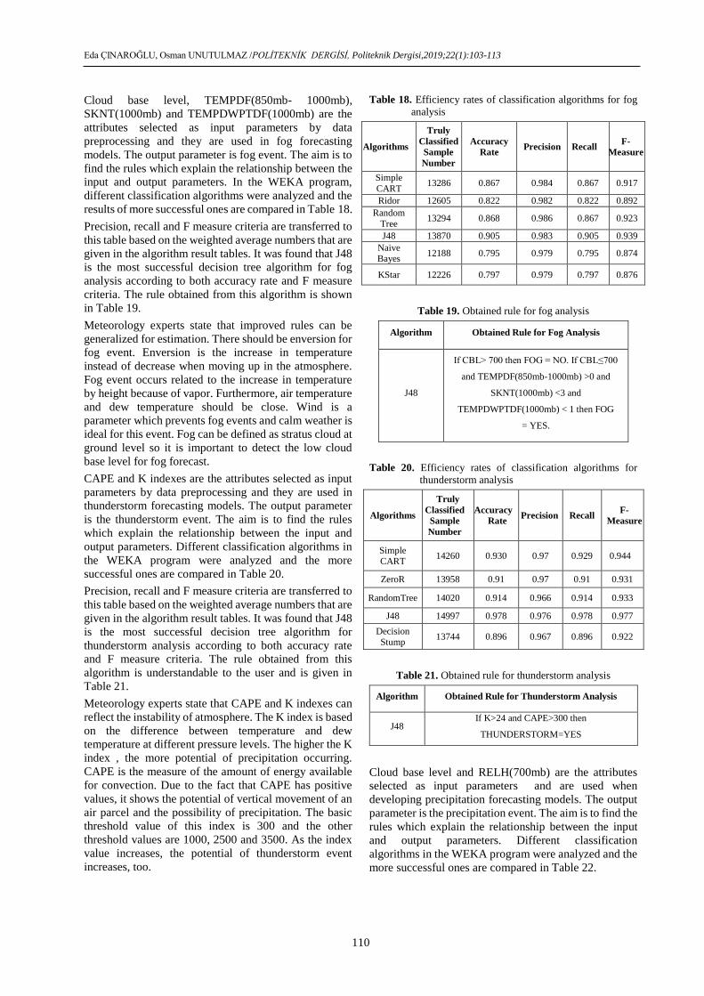
Cloud base level, TEMPDF(850mb- 1000mb),
SKNT(1000mb) and TEMPDWPTDF(1000mb) are the
attributes selected as input parameters by data
preprocessing and they are used in fog forecasting
models. The output parameter is fog event. The aim is to
find the rules which explain the relationship between the
input and output parameters. In the WEKA program,
different classification algorithms were analyzed and the
results of more successful ones are compared in Table 18.
Precision, recall and F measure criteria are transferred to
this table based on the weighted average numbers that are
given in the algorithm result tables. It was found that J48
is the most successful decision tree algorithm for fog
analysis according to both accuracy rate and F measure
criteria. The rule obtained from this algorithm is shown
in Table 19.
Meteorology experts state that improved rules can be
generalized for estimation. There should be enversion for
fog event. Enversion is the increase in temperature
instead of decrease when moving up in the atmosphere.
Fog event occurs related to the increase in temperature
by height because of vapor. Furthermore, air temperature
and dew temperature should be close. Wind is a
parameter which prevents fog events and calm weather is
ideal for this event. Fog can be defined as stratus cloud at
ground level so it is important to detect the low cloud
base level for fog forecast.
CAPE and K indexes are the attributes selected as input
parameters by data preprocessing and they are used in
thunderstorm forecasting models. The output parameter
is the thunderstorm event. The aim is to find the rules
which explain the relationship between the input and
output parameters. Different classification algorithms in
the WEKA program were analyzed and the more
successful ones are compared in Table 20.
Precision, recall and F measure criteria are transferred to
this table based on the weighted average numbers that are
given in the algorithm result tables. It was found that J48
is the most successful decision tree algorithm for
thunderstorm analysis according to both accuracy rate
and F measure criteria. The rule obtained from this
algorithm is understandable to the user and is given in
Table 21.
Meteorology experts state that CAPE and K indexes can
reflect the instability of atmosphere. The K index is based
on the difference between temperature and dew
temperature at different pressure levels. The higher the K
index , the more potential of precipitation occurring.
CAPE is the measure of the amount of energy available
for convection. Due to the fact that CAPE has positive
values, it shows the potential of vertical movement of an
air parcel and the possibility of precipitation. The basic
threshold value of this index is 300 and the other
threshold values are 1000, 2500 and 3500. As the index
value increases, the potential of thunderstorm event
increases, too.
Table 18. Efficiency rates of classification algorithms for fog
analysis
Algorithms
Truly
Classified
Sample
Number
Accuracy
Rate Precision Recall
F-
Measure
Simple
CART 13286 0.867 0.984 0.867 0.917
Ridor 12605 0.822 0.982 0.822 0.892
Random
Tree 13294 0.868 0.986 0.867 0.923
J48 13870 0.905 0.983 0.905 0.939
Naive Bayes
12188 0.795 0.979 0.795 0.874
KStar 12226 0.797 0.979 0.797 0.876
Table 19. Obtained rule for fog analysis
Algorithm Obtained Rule for Fog Analysis
J48
If CBL> 700 then FOG = NO. If CBL≤700
and TEMPDF(850mb-1000mb) >0 and
SKNT(1000mb) <3 and
TEMPDWPTDF(1000mb) < 1 then FOG
= YES.
Table 20. Efficiency rates of classification algorithms for
thunderstorm analysis
Algorithms
Truly
Classified
Sample
Number
Accuracy
Rate Precision Recall
F-
Measure
Simple CART
14260 0.930 0.97 0.929 0.944
ZeroR 13958 0.91 0.97 0.91 0.931
RandomTree 14020 0.914 0.966 0.914 0.933
J48 14997 0.978 0.976 0.978 0.977
Decision Stump
13744 0.896 0.967 0.896 0.922
Table 21. Obtained rule for thunderstorm analysis
Algorithm Obtained Rule for Thunderstorm Analysis
J48 If K>24 and CAPE>300 then
THUNDERSTORM=YES
Cloud base level and RELH(700mb) are the attributes
selected as input parameters and are used when
developing precipitation forecasting models. The output
parameter is the precipitation event. The aim is to find the
rules which explain the relationship between the input
and output parameters. Different classification
algorithms in the WEKA program were analyzed and the
more successful ones are compared in Table 22.
A DATA MINING APPLICATION OF LOCAL WEATER FORECAST FOR KAYSERİ ERKI… Politeknik Dergisi, 2019; 22 (1) : 103-113
111
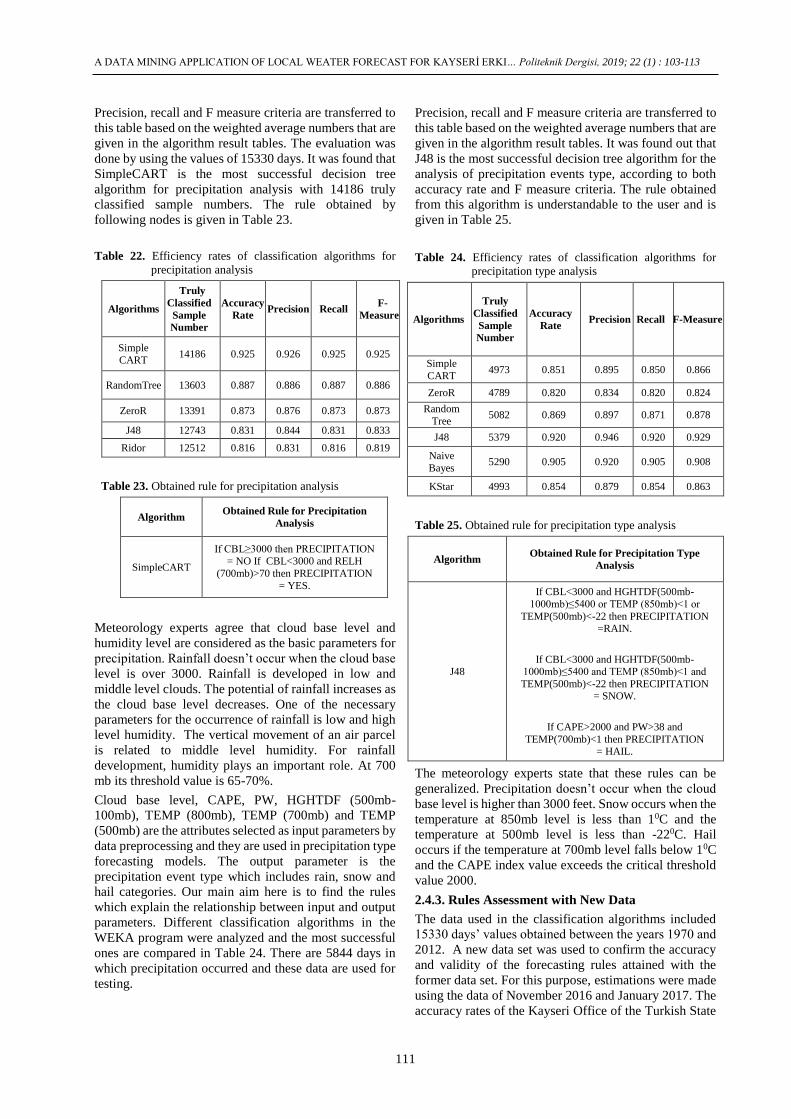
Precision, recall and F measure criteria are transferred to
this table based on the weighted average numbers that are
given in the algorithm result tables. The evaluation was
done by using the values of 15330 days. It was found that
SimpleCART is the most successful decision tree
algorithm for precipitation analysis with 14186 truly
classified sample numbers. The rule obtained by
following nodes is given in Table 23.
Table 22. Efficiency rates of classification algorithms for
precipitation analysis
Algorithms
Truly
Classified
Sample
Number
Accuracy
Rate Precision Recall
F-
Measure
Simple
CART 14186 0.925 0.926 0.925 0.925
RandomTree 13603 0.887 0.886 0.887 0.886
ZeroR 13391 0.873 0.876 0.873 0.873
J48 12743 0.831 0.844 0.831 0.833
Ridor 12512 0.816 0.831 0.816 0.819
Table 23. Obtained rule for precipitation analysis
Algorithm Obtained Rule for Precipitation
Analysis
SimpleCART
If CBL≥3000 then PRECIPITATION = NO If CBL<3000 and RELH
(700mb)>70 then PRECIPITATION
= YES.
Meteorology experts agree that cloud base level and
humidity level are considered as the basic parameters for
precipitation. Rainfall doesn’t occur when the cloud base
level is over 3000. Rainfall is developed in low and
middle level clouds. The potential of rainfall increases as
the cloud base level decreases. One of the necessary
parameters for the occurrence of rainfall is low and high
level humidity. The vertical movement of an air parcel
is related to middle level humidity. For rainfall
development, humidity plays an important role. At 700
mb its threshold value is 65-70%.
Cloud base level, CAPE, PW, HGHTDF (500mb-
100mb), TEMP (800mb), TEMP (700mb) and TEMP
(500mb) are the attributes selected as input parameters by
data preprocessing and they are used in precipitation type
forecasting models. The output parameter is the
precipitation event type which includes rain, snow and
hail categories. Our main aim here is to find the rules
which explain the relationship between input and output
parameters. Different classification algorithms in the
WEKA program were analyzed and the most successful
ones are compared in Table 24. There are 5844 days in
which precipitation occurred and these data are used for
testing.
Precision, recall and F measure criteria are transferred to
this table based on the weighted average numbers that are
given in the algorithm result tables. It was found out that
J48 is the most successful decision tree algorithm for the
analysis of precipitation events type, according to both
accuracy rate and F measure criteria. The rule obtained
from this algorithm is understandable to the user and is
given in Table 25.
Table 24. Efficiency rates of classification algorithms for
precipitation type analysis
Algorithms
Truly
Classified
Sample
Number
Accuracy
Rate Precision Recall F-Measure
Simple
CART 4973 0.851 0.895 0.850 0.866
ZeroR 4789 0.820 0.834 0.820 0.824
Random
Tree 5082 0.869 0.897 0.871 0.878
J48 5379 0.920 0.946 0.920 0.929
Naive
Bayes 5290 0.905 0.920 0.905 0.908
KStar 4993 0.854 0.879 0.854 0.863
Table 25. Obtained rule for precipitation type analysis
Algorithm Obtained Rule for Precipitation Type
Analysis
J48
If CBL<3000 and HGHTDF(500mb-
1000mb)≤5400 or TEMP (850mb)<1 or
TEMP(500mb)<-22 then PRECIPITATION =RAIN.
If CBL<3000 and HGHTDF(500mb-1000mb)≤5400 and TEMP (850mb)<1 and
TEMP(500mb)<-22 then PRECIPITATION = SNOW.
If CAPE>2000 and PW>38 and
TEMP(700mb)<1 then PRECIPITATION = HAIL.
The meteorology experts state that these rules can be
generalized. Precipitation doesn’t occur when the cloud
base level is higher than 3000 feet. Snow occurs when the
temperature at 850mb level is less than 10C and the
temperature at 500mb level is less than -220C. Hail
occurs if the temperature at 700mb level falls below 10C
and the CAPE index value exceeds the critical threshold
value 2000.
2.4.3. Rules Assessment with New Data
The data used in the classification algorithms included
15330 days’ values obtained between the years 1970 and
2012. A new data set was used to confirm the accuracy
and validity of the forecasting rules attained with the
former data set. For this purpose, estimations were made
using the data of November 2016 and January 2017. The
accuracy rates of the Kayseri Office of the Turkish State
Eda ÇINAROĞLU, Osman UNUTULMAZ /POLİTEKNİK DERGİSİ, Politeknik Dergisi,2019;22(1):103-113
112
Meteorological Service regarding these meteorological
events were obtained from the forecasting and warning
center authoritative. The comparisons of results among
the estimations, real meteorological events and estimates
of the Kayseri Regional Office are as follows:
Fog event occurred on 42 days out of 61 days of
observation. Fog on 40 days was correctly estimated
by the obtained rules. Fog didn’t occur on 19 of 61
days of observation. Of these 19 days, estimation was
correct on 14 days. The fog analysis had a success rate
of 89%. The accuracy rate of fog event obtained by
the Kayseri Regional Office was observed as 85% for
these two months.
Thunderstorm event didn’t occur during the 61 days
of observation. All estimations were totally correct.
The thunderstorm analysis had a success rate of
100%. The accuracy rate of thunderstorm event
obtained by the Kayseri Regional Office was
observed as 100% for these two months.
Precipitation event occurred on 18 of 61 days of
observation. It was correctly estimated on 16 days by
the obtained rules. Precipitation event didn’t occur on
43 of 61 days of observation. Of these 43 days,
estimation was correct on 39 days. The precipitation
analysis had a success rate of 90.2%. The accuracy
rate of precipitation event obtained by the Kayseri
Regional Office was observed as 89.1% for these two
months.
3. RESULTS AND DISCUSSION
Risk is a factor that must be minimized to the lowest
degree for the aviation sector. For this reason, decisions
should be taken according to meteorological information.
Understanding meteorological events is only possible
with the observation of many parameters which are
related to each other. Previous mass data should be
overviewed for the future forecast. Expert opinions are
also necessary in the analysis process. At this point, it is
believed that data mining makes a great contribution to
the analysis of mass data and it increases the rate of
accuracy and speed.
This study aims at revealing the correlation between
meteorological parameters that affect aviation and
finding rules by classification. The basic benefits of the
study are the usage of high level values without maps and
expert opinion, obtaining the local forecast for Kayseri
Erkilet Airport and mining rules for the estimation of fog,
precipitation and thunderstorm events.
The user can simply understand and interpret these rules.
They can be used for future forecasts without expert
opinion.
The study proves that data mining is a suitable method
for meteorological data analysis. Rules may be formed
for other different meteorological events by enlarging the
concept of analysis in future studies.
REFERENCES
[1] Hand D., Mannila H. and Smyth P., “Principles of data
mining”, The Mit Press, England, (2001).
[2] Akpınar H., “Veri tabanlarında bilgi keşfi ve veri
madenciliği”, İstanbul Üniversitesi İşletme Fakültesi
Dergisi, 29: 1-22, (2000).
[3] Han J. and Kamber M., “Data mining: concepts and
techniques”, Morgan Kaufmann Publishers, USA,
(2001).
[4] Fayyad U., Piatetsky-Shapiro G. and Smyth P., “From
data mining to knowledge discovery in databases”,
American Association for Artificial Intelligence, 37-54,
(1996).
[5] Özekes S., “Veri madenciliği modelleri ve uygulama
alanları”, İstanbul Ticaret Üniversitesi Dergisi, 4: 65-82,
(2003).
[6] Allen G. and LeMarchall J., “An evaluation of neural
networks and discriminant analysis methods for
application in operational rain forecasting”, Australian
Meteorological Magazine, 43: 17-28, (1994).
[7] McGullagh J., Choi B. and Bluff K., “Genetic evolution
of a neural networks input vector for meteorological
estimations”, ICONIP’97, New Zealand 1046-1049,
(1997).
[8] Stern H. and Parkyn K., “Predicting the likelihood of fog
at Melbourne Airport”, 8th Conference on Aviation,
Range and Aerospace Meteorology, American
Meteorological Society, Dallas, 174-178, (1999).
[9] Mitsukura Y., Fukumi M. and Akamatsu N., “A design of
genetic fog occurrence forecasting system by using LVQ
network”, Proc. of IEEE SMC'2000, USA, 3678-3681,
(2000).
[10] Trafalis T. B., Richman M. B. and A. White A., “Data
mining techniques for improved WSR-88D rainfall
estimation”, Computers & Industrial Engineering, 43:
775-786, (2002).
[11] Solomatine D. and Dulal K. N., “Model trees as an
alternative to neural networks in rainfall—runoff
modelling”, Hydrological Sciences Journal, 48: 399-
411, (2003).
[12] Lee R. and Liu J., “iJADEWeatherMAN: A weather
forecasting system using intelligent multiagent-based
fuzzy neuro network”, IEEE Transactions On Systems,
Man and Cybernetics – Part C: Applications and
Reviews, 34: 369-377, (2004).
[13] Jareanpon C., Pensuwon W. and Frank R. J., “An
adaptive RBF network optimised using a genetic
algorithm applied to rainfall forecasting”, International
Symposium on Communications and Information
Technologies 2004 (ISCK 2004), 1005-1010, Japan,
(2004).
[14] Suvichakorn A. and Tatnall A., “The application of cloud
texture and motion derived from geostationary satellite
images in rain estimation—A study on mid-latitude
depressions”, Geoscience and Remote Sensing
Symposium, 1682-1685, (2005).
[15] Banik S., Anwer M., Khan K., Rouf R. A. and Chanchary
F. H., “Neural network and genetic algorithm approaches
for forecasting Bangladeshi monsoon rainfall”,
Proceedings of 11th International Conference on
A DATA MINING APPLICATION OF LOCAL WEATER FORECAST FOR KAYSERİ ERKI… Politeknik Dergisi, 2019; 22 (1) : 103-113
113
Computer and Information Technology (ICCIT 2008),
Khulna-Bangladesh, 735-740, (2008).
[16] Pan X. and Wu J., “Bayesian neural network ensemble
model based on partial least squares regression and its
application in rainfall forecasting”, 2009 International
Joint Conference on Computational Sciences and
Optimization, Chine, 49-52, (2009).
[17] Aktaş C. and Erkuş O., “Lojistik regresyon analizi ile
Eskişehir’in sis kestiriminin incelenmesi”, İstanbul
Ticaret Üniversitesi Fen Bilimleri Dergisi, 16: 47-59,
(2009).
[18] Bartok J., Habala O., Bednar P., Gazak M. and Hluchy
L., “Data mining and integration for predicting significant
meteorological phenomena”, Procedia Computer
Science, 1: 37-46, (2010).
[19] Zazzaro G., Pisano F. M. and Mercogliano P., “Data
mining to classify fog events by applying cost-sensitive
classifier”, 2010 International Conference on Complex,
Intelligent and Software Intensive Systems, Poland,
(2010).
[20] Wu J., “An effective hybrid semi–parametric regression
strategy for artificial neural network ensemble and its
application rainfall forecasting”, 2011 Fourth
International Joint Conference on Computational
Sciences and Optimization, China, 1324-1328, (2011).
[21] Lee S. E. and Seo K. H., “The development of a statistical
forecast model for Changma”, Weather and Forecasting,
28: 1304-1321, (2013).
[22] Agrawal R., Imielinski T. and Swami A., "Mining
associations between sets of items in large databases",
ACM SIGMOD Int'l Conf. on Management of Data,
Washington D.C., 207-216, (1993).
[23] Giudici, P., “Applied data mining statistical methods for
business and industry”, John Wiley&Sons Ltd., England,
(2003).
[24] Baykal A. and Coşkun C., “Veri madenciliğinde
sınıflandırma algoritmalarının bir örnek üzerinde
karşılaştırılması”, Akademik Bilişim, Malatya,
http://ab.org.tr/ab11/bildiri/67.pdf, (2011).