A Data-Driven Stochastic Method

Mulin Cheng, Thomas Y. Hou, Pengchong YanApplied and Computational Mathematics,

California Institute of Technology, Pasadena, CA 91106

Abstract

Stochastic partial differential equations (SPDE) arise in many physical and engineering applications.Solving these SPDE efficiently and accurately presents a great challenge. The Wiener Chaos Expansionmethod (WCE) and its variants have shown some promising features but still suffer from the slow conver-gence of polynomial expansion and the curse of dimensionality. The Monte Carlo method (MC) has anattractive property that its convergence is independent of the number of stochastic dimensions. However,its convergence rate is only of order O(1/

√N) (N is the number of realizations). Inspired by Multi-scale

Finite Element methods (MsFEM) and Proper Orthogonal Decomposition methods, we propose a data-drivenstochastic method, which consists of offline step and online step and uses both MC and WCE. A randombasis Ai(ω)Mi=1 is computed in the offline step based on the Karhunen-Loeve(KL) expansion, which can beviewed as partially inversion of the random differential operator. In the online step, the polynomial basis usedin Polynomial Chaos expansion is replaced by the problem-dependent stochastic basis that we constructedin the offline step. By solving a set of coupled deterministic PDEs of coefficients, we obtain the numericalsolutions of SPDEs. The proposed framework is applied to 1D and 2D elliptic problems with random coef-ficients and a horn problem. Numerical examples show that 1. The stochastic basis obtained in the offlinecomputation can be repeatedly used in the online computation for different deterministic right hand sides.2. A much smaller number of bases are necessary in the online computation to achieve certain error tolerancecompared to WCE.

1 IntroductionUncertainty arises in many complex real-world problems of physical and engineering interests, such as wave,heat and pollution propagation through random media, randomly forced Burgers or Navier-Stokes equations.Additional examples can be found extensively in other branches of science and engineering, such as fluid dy-namics, geophysics, quantum mechanics, statistical physics, biology and etc. Stochastic Partial differentialequation(SPDE) is an effective mathematical tool to model these complicated problems, which manifests ran-domness in many aspects, such as initial/boundary conditions, model parameters, measurements, to name afew. Solving these SPDEs poses a great challenge to the scientific computing community.

In many applications, one is mostlt interested in statistical information of the stochastic solution. For thispurpose, people have derived moment equations and probability density function (PDF) methods in whicheffective equations such as Fokker-Planck equations, have been derived for the moments and the PDF. Fornonlinear problems, such methods suffer from the closure problem. Because of stability and non-intrusivenature of the Monte Carlo method(MC), it remains the most popular numerical method for SPDEs. Due to thelaw of large number, the convergence rate of MC is merely 1√

N[?], where N is the number of realizations.

There are various ways to accelerate the convergence rate of MC by using variation reduction techniques, suchas anti-thetic variables, conditioning, control variates, and importance sampling. For SPDEs, one can also usecollocation and sparse grid methods to reduce the complexity of the method, but none of these techniques canchange the nature of slow convergence of MC.

While MC method represents the solution of SPDE as an ensemble of realizations, another way to representthe solution is to expand it in an orthonormal basis, or polynomial chaos which was originally proposed by N.Wiener in 1938[?]. The method did not receive much attention until Cameron and Martin developed an explicit

1

and intuitive formulation for Wiener Chaos Expansion(WCE) in their elegant work in 1947. Compared toMC methods, dramatic improvements can be achieved in some problems, but WCE method has two maindisadvantages

1. The number of terms in truncated WCE grows exponentially fast as the order of Hermite polynomialsand the number of random variables increase, especially for long time integration.

2. The solution may depend sensitively on random dimensions, such as parameter shocks or bifurcation,which further demands more terms in WCE.

To reduce dimensionality and achieve sparse representation, several generalizations of the classical WCEmethod have been proposed to circumvent the drawbacks, such as generalized polynomial chaos via Wiener-Askey polynomial [?], Wiener-Haar Chaos Expansion [?], Multi-element gPC [?, ?, ?] and etc. Improvementsare observed in some problems, but not all, especially for time-dependent problems. It is important to note thatthe basis used in the polynomial chaos expansion is determined a prior and problem independent, which webelieve is the ultimate reason of giving rise to a non-sparse representation of the stochastic solution when thesolution is not smooth in the stochastic space or when the stochastic dimension is high.

A typical scenario occurring frequently in practice is that we are interested in investigating what will happenwhen deterministic parts of the problem change and the random parts remain unchanged. For example, theproperties of certain kind of composite material satisfy some stochastic processes with known parameters andwe want to know its responses under different external forces. Mathematically, consider the SPDE in thegeneral form of

L(ω)u(x, ω) = f(x)

where x ∈ D, ω ∈ Ω and L(ω) is a stochastic differential operator. Clearly, L(ω) represents the randomparts of the problem while f(x) is the deterministic part of the problem. Our framework can be extended totime-dependent SPDE which we should address in a separate paper. The method we proposed consists twoparts:

• Offline: The stochastic basis Ai(ω) is constructed based on the Karhunen-Loeve(KL) expansion ofMCFEM solutions u(x, ω) for a specific right-hand side f(x) = f0(x).

• Online: For the right-hand side f(x) of interests, the solution is projected on the constructed basis,

u(x, ω) ≈M∑i=0

ui(x)Ai(ω)

where A0 = 1. By Galerkin projection, a system of coupled deterministic PDEs of ui(x, t) can obtainedand solved numerically. The mean, variance and other statistical quantities can be recovered from thesolution of ui(x, t).

This paper is organized as follows. In the next two section, Offline and online algorithms will be describedand analyzed in details along with Multi-Level Monte Carlo Method to accelerate offline computation. Insec.5, we applied our method to elliptic partial differential equations with random elliptic coefficients andcompared the results with those by PC method to show the advantages. Some cases of physical and engineeringinterests, such as large variance or jumps at random locations, are also included and analyzed numerically indetails. To demonstrate the potential application of our method in industrial/realistic scenario, a horn problemis considered. Some concluding remarks are given in Section 6.

2

2 Theory

2.1 Stochastic Partial Differential EquationConsider the stochastic PDE, linear or non-linear, in the general form of

L(x, ω)u(x, ω) = f0(x), x ∈ D, ω ∈ Ω

u(x, ω) = 0, x ∈ ∂D, (2.1)

or

L(x, ω)u(x, ω) = 0, x ∈ D, ω ∈ Ω

u(x, ω) = f0(x), x ∈ Γ ⊆ ∂D, (2.2)

where D is a d-dimensional physical space. Here the deterministic function f0(x) exists either at the right-hand-side of the PDE, or as part of the boundary condition.

The Monte-Carlo solution of the elliptic equation, given one sample ω, u(x, ω) is solved. The Karhunen-Loeve decomposition of the PDE solution gives the dominant components in the random spaces. We denotethe KL decomposition as

u(x, ω; f0) = u(x; f0) +

∞∑i=1

√λiAi(ω)φi(x; f0), (2.3)

where u(x; f0) = Eu(x, ω; f0). In the current paper, we intend to derive the empirical basis Ai(ω)i=1,...,M

based on a test function f0(x), where M is a small truncation number. Notice that the basis Ai(ω)i=1,...,M

in the KL decomposition are orthonormal basis. We don’t need to store all information of Ai(ω), but somemoments, such as E[a(x, ω)Ai(ω)Aj(ω)]. Those computations can be done off-line. Then for a differentfunction f1(x), we are looking for a Galerkin projection of the solution, i.e.,

u(x, ω; f1) = u(x; f1) +

M∑i=1

Ai(ω)ui(x; f1). (2.4)

For easy notation, we denote A0(ω) = 1 and u0(x; f1) = u(x; f1).It is important to point that if the correlation length of the solution is small, then the number of basis M

may be large due to the large dimension of the stochastic solution space. Then our method is not an optimalchoice to solve the problem, although it still has its big advantages over other method, such as WCE. In thispaper, we will exclude this situation and consider only the case with large correlation length of the solution.

In addition to that, there exists some puzzles here we need to solve here. As for the Wiener Chaos expansion,the dimension of the stochastic domain is infinite, while we only choose a PDE-driven stochastic domain, whichis very small (if the variance of the solution is not large). In order to validate the Galerkin method, we will

1. verify the dominant solution space is finite dimensional;

2. define a class of recoverable function f1(x) on the basis generated off-line by f0(x).

2.2 Solution space of 1D Elliptic equation with random coefficientsLet’s first consider the stochastic Elliptic equation of the form

− div(a(x, ω)Ou) = f0(x), x ∈ D, ω ∈ Ω

u(x, ω) = 0, x ∈ ∂D (2.5)

3

where D = [0, 1]d, d is the space dimension, and a(x, ω) is a random variable satisfying the ellipticity, 0 <a0 ≤ a(x, ξ) ≤ a1 <∞. In particular, we consider the simple 1-d case with homogeneous Dirichlet boundarycondition:

∂

∂x(a(x, ω)

∂

∂xu(x, ω)) = −f(x).

Then we derive

a(x, ω)∂

∂xu(x, ω) = −

∫ x

0

f(s1)ds1 + C(ω),

where C(ω) is determined by the boundary conditions. In addition, we denote b(x, ω) = (a(x, ω))−1. Thenthe solution is given by

u(x, ω) = −∫ x

0

b(s2, ω)( ∫ s2

0

f(s1)ds1 − C(ω))ds2.

Because of the boundary condition u(1, ω) = 0, we have

C(ω) =

∫ 1

0b(s1, ω)

∫ s10f(s2)ds2ds1∫ 1

0b(s, ω)ds

. (2.6)

Also we can write the Karhunen-Loeve decomposition of b(x, ω) as

b(x, ω) =

M∑i=0

bi(x)Bi(ω),

in which we only keep the first M leading terms. Then the solution is

u(x, ω) = −∫ x

0

∑i

bi(s2)Bi(ω)

∫ s2

0

f(s1)ds1

+( ∫ x

0

∑i

bi(s)Bi(ω)ds)∫ 1

0

∑j bj(s1)Bj(ω)

∫ s10f(s2)ds2ds1∫ 1

0b(s, ω)ds

.

Apparently, the stochastic part of first term lies in the space spanned by Bi(ω)i=1,...,M , while that of thesecond one lies in the space spanned byBi(ω)Bj(ω)∫ 1

0b(s, ω)ds

i,j

with i, j = 0, 1, . . . ,M.

Again we denote B0 = 1. Then the solution of the 1-d Stochastic elliptic equation lies in the same stochasticspace, which is independent of the right-hand-side function f(x).

2.3 Solution space of 2D and higher dimensional elliptic equation with random coffi-cients

In high-dimension case, we consider the Green’s function G(x, y;ω), which satisfies

− div(a(x, ω)OG(x,y;ω)) = δ(x− y), x,y ∈ D, ω ∈ Ω

G(x,y;ω) = 0, x ∈ ∂D, y ∈ D. (2.7)

Again we can write out the Karhunen-Loeve decomposition of G(x,y;ω)

G(x,y;ω) =

M∑i=0

Gi(x,y)ξi(ω),

4

in which we keep the leading M terms. Then solution of the elliptic equation is

u(x, ω) =

∫D

G(x,y;ω)f(y)dy

=

M∑i=0

(∫D

Gi(x,y)f(y)dy)ξi(ω).

So again the solution lies in a finite dimensional stochastic space spanned by ξi(ω)i=1,...,M , regardless ofthe right-hand-side f(x).

Although this part is derived for Elliptic equation, the results can be generalized to a large class of stochasticPDEs (e.g., those PDE with a Green’s function, see Helmholtz equation in Sec.5.3).

3 Data-Driven Stochastic Multi-scale MethodThe central task of our method is to look for a Data-Driven or Problem-Dependent random basis under whichsolutions enjoy a sparse expansion. The Error-Minimizing property of Karhunen-Loeve (KL) expansion makesit a natural choices. Specifically, for u(x, ω) ∈ L2(D × Ω), its Karhunen-Loeve expansion is

u(x, ω) = E [u] +

∞∑i=1

√λiξi(ω)φi(x)

where λi and φi(x) are the eigenvalue and the eigenfunction of the covariance kernel C(x, y), i.e.,∫D

C(x, y)φ(y)dy = λφ(x)

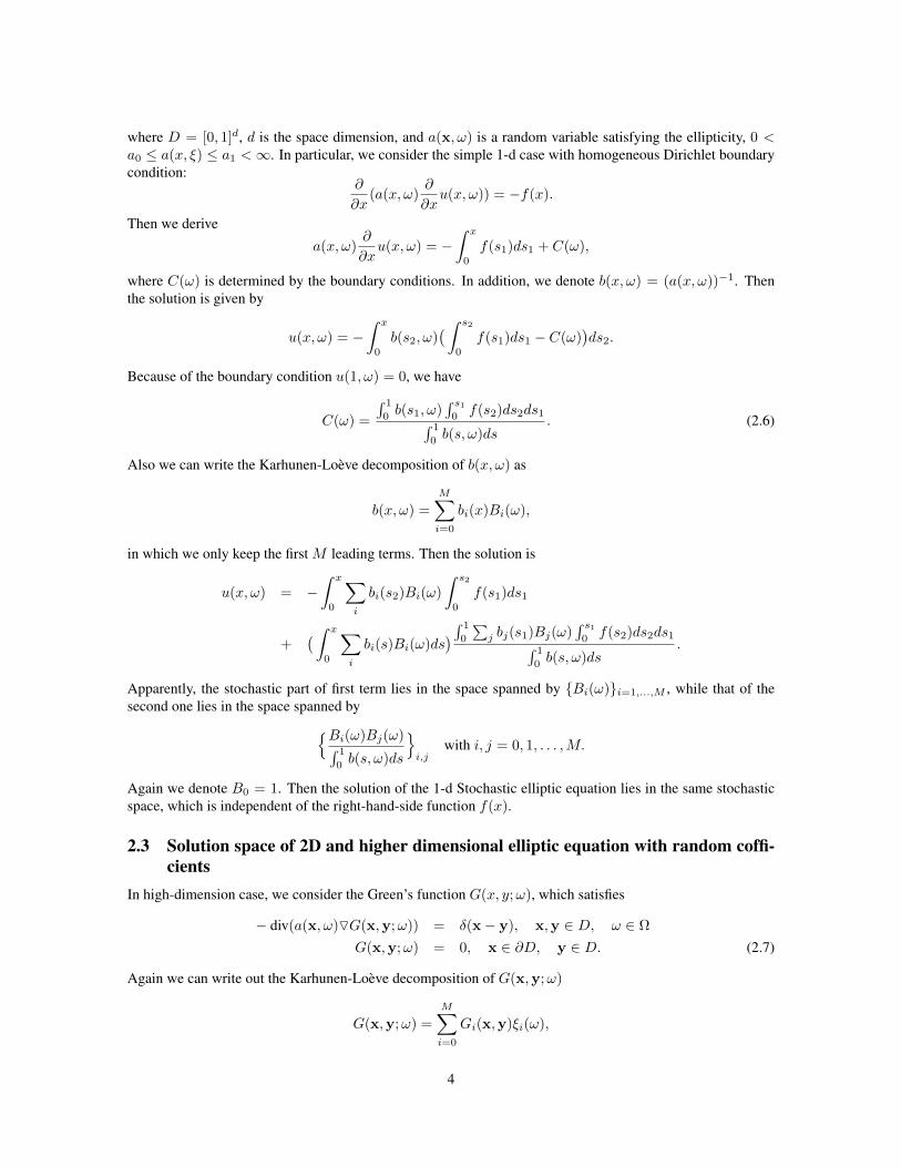
where C(x, y) = E [(u(x, ω)− E [u(x, ·)])(u(y, ω)− E [u(y, ·)])]. Under some general conditions, the eigen-values in KL expansion decay exponentially fast [?], which means the first few terms, or modes, of the KLexpansion can give very good approximation of u(x, ω). In other words, the dimension of input random spacemay be large, but the dimension of the effective output random space may be much smaller as shown in fig.1.

For elliptic PDE, a heuristic argument based on Green’s function shows the properties of solutions aremainly controlled by the properties of stochastic differential operatorL(ω). Therefore, the solutions u(x, ω) fora board class of right-hand side f(x) may enjoy sparse representation under some random basis which certainlydepends on the stochastic operator L(ω). In other words, a random basis computed for a specific deterministicright-hand side f(x) = f0(x) may provide sparse representations for a board class of deterministic right-hand side f(x). Similar philosophy has been adopted in Multi-scale Finite Element methods [?] and ProperOrthogonal Decomposition (POD) methods [?, ?, ?], so we name our method as Data-Driven Stochastic Multi-scale method.

3.1 Offline and Online PartsIf we follow this philosophy, the framework we proposed naturally breaks into two parts, the constructionof a random basis Ai(ω)Mi=1 and the numerical solution of a coupled system of PDEs of the expansioncoefficients. For a fixed stochastic differential operator L(ω), the computation of the random basis may beexpansive depending on the problem and the accuracy requirements. Once the random basis are constructed,they can be used repeated for different right-hand side function f(x).r Therefore, we call the construction ofrandom basis the offline computation part, meaning this step is a preprocess step and can be completed in an“offline” manner contrast to the numerical solution of a coupled system of PDEs in an “online” manner. Thefollowing two algorithms reveal the details of each parts.

The goal of offline computation is to construct the random basis based on KL expansion of the randomsolution. The algorithm formulated below is essentially two-pass Monte Carlo method. In the first pass, the

5

0 5 10 15 2010

−15

10−10

10−5

100

β = 3.0

M = 05M = 10M = 15M = 20

0 5 10 15 2010

−14

10−12

10−10

10−8

10−6

10−4

10−2

β = 2.0

M = 05M = 10M = 15M = 20

0 5 10 15 2010

−12

10−10

10−8

10−6

10−4

β = 1.0

M = 05M = 10M = 15M = 20

0 5 10 15 2010

−12

10−10

10−8

10−6

10−4

β = 0.0

M = 05M = 10M = 15M = 20

Figure 1: Eigenvalues of the covariance function of solutions for elliptic PDE with random coefficientsa(x, ω) =

∑Mm=1m

−βξm(sin(2πmx + ηi) + 1), where ξi’s, ηi’s are independent uniform random variableson [0, 1]. We observe that the dimensionality of input random space may be large, but effective output randomspace may be much smaller due the exponential convergence of eigenvalues of covariance function.

mean and the covariance function of the solution are computed. In the second pass, the random basis and theirrelevant statistical information are computed. Various Monte Carlo acceleration techniques can be integratedinto this step and reduce the offline computational cost, which is relevant, but not the central focus of this paper.

Algorithm 1 (Offline Computation).

1. Compute the expectation u = E [u] and the covariance functionR(x, x′) = E [(u(x, ω)− u(x))(u(x′, ω)− u(x′))]by Monte Carlo Method with N1 realizations, i.e.,

u(x) =1

N1

N1∑n=1

u(x, ωn)

R(x, x′) =1

N1u(x, ωn)u(x′, ωn)− u(x)u(x′)

2. Solve the first M pairs of eigenvalues and eigenfunctions

λiφi(x) =

∫D

R(x, x′)φi(x′) dx′, i = 1, . . . ,M

6

3. Compute the stochastic basis Ai(ω) by

Ai(ω) =1√λi

∫D

u(x, ω)φi(x) dx

and statistical information of Ai(ω), such as

E [AiAjAk] =1

N2

N2∑n=1

Ai(ωn)Aj(ωn)Ak(ωn)

Remark 3.1. Guard-lines of selections for computational parameters. The decaying property of eigenvaluescan be used to select parameter M , i.e., the number of random basis M can be chosen such as λM+1

λ1is small.

In general, N1 can be chosen to be smaller than N2.

Remark 3.2. In the online part, Galerkin projection reduces the stochastic PDE to a coupled system of PDEswhose coefficients involve only of statistical information of Ai(ω)’s, such as E [AiAjAk], which suggests onlysuch information be stored in the offline part.

Remark 3.3. Our method is semi-non-intrusive in the sense that certified legacy codes can be used with mini-mum changes in offline part. This property makes it very attractive to industrial community as it reuses codesverified by possibly expansive and time-consuming experiments and avoid another life cycle of developing newprograms.

Remark 3.4. We can apply multi-level techniques to speed-up the construction of random basis which will bedetailed in the next section.

Once the random basis is constructed and stored, we are ready to apply it to cases which we really interestedin. The constructed random basis spans a finite-dimensional subspace in L2(Ω) and we can project the solutionu(x, ω) on this subspace, and write

u(x, ω) ≈M∑i=0

ui(x)Ai(ω) (3.1)

where A0 = 1. We include A0 in the random basis to make the formulation concise. The expanded randombasis Ai(ω)Mi=0 can be verified to be orthonormal. In this paper, we mainly consider elliptic-type PDEwith random coefficients. To demonstrate the main idea of online part, we consider elliptic PDE with randomcoefficients and homogeneous boundary conditions are assumed, i.e.,

− ∂

∂xp

(apq(x, ω)

∂u

∂xq(x, ω)

)= f(x), x ∈ D ⊂ Rd

u(x, ω) = 0, x ∈ ∂D

where p, q = 1, . . . , d, Einstein summation is assumed and

L(ω) = − ∂

∂xp

(apq(x, ω)

∂

∂xq(x, ω)·

)Similar formulations can be obtained for other types of stochastic differential operator.

Algorithm 2 (Online Computation).

1. expand the solution under the random basis Ai(ω), substitute into the SPDE, multiply both side byAj(ω) and take expectations, i.e., Galerkin projection, which gives a set of PDEs for ui(x).

− ∂

∂xp

(E [apqAiAj ]

∂ui∂xq

)= f(x), x ∈ D, i, j = 0, 1, . . . ,M

ui(x) = 0, x ∈ ∂D

7

2. Solve the coupled system of deterministic PDEs by numerical methods, such as Finite Element Method,Finite Difference Method and etc.

3. Statistical information of the solution which are of primary interests can be calculated from deterministiccoefficients. For example, the centered fourth moment can be computed as

E[(u− u)4

]=∑i,j,k,l

E [AiAjAkAl]uiujukul

where E [AiAjAkAl] is readily available in the offline part.

Remark 3.5. Besides statistical information of solutions, sometimes other types of information, such as extremeevents and etc, is desired, which requires distribution information of solutions. In such cases, instead of storingonly the statistical information of the random basis Ai(ω)Mi=1, we may exploring their sparse representationunder some predefined random basis, such as polynomial chaos basis, Haar chaos basis and etc and store theoffline-constructed random basis completely. This part constitutes parts of ongoing work.

3.2 Complexity AnalysisThe applicability of our method depends on the dimension of the stochastic space that the solution lies in. If thedimension is large, we have to choose more stochastic bases and hence increase the complexity of the Galerkinprojection.

Proposition 3.1. [?] If we consider the Gaussian covariance kernels of the form

R(x, x′) = σ2 exp(−|x− x′|2/γ2),

then the eigenvalues λm has the properties

0 ≤ λm ≤ σ2 (1/γ)m1/d+2

Γ(0.5m1/d), ∀m ≥ 1,

where x lies in a unit d−dimensional domain, and Γ is the gamma function.

It is clear that the larger correlation length γ, the slower decaying of the eigenvalues. Consequently in ourDSMM, we have to adopt more bases because of the effective dimension increasing. Hence it will worse theefficiency of our method.

4 Multi-Level Monte Carlo AccelarationAlthough the offline computation may be expansive, the constructed random basis can be stored and usedrepeatedly in online computation for different cases. Various variance reduction techniques can be used toaccelerate the offline computation, among which Multi-Level Monte Carlo method (MLMC) has been provedto be very effective for stochastic differential equation [?]. Here we will demonstrate the applicability of theMLMC to SPDE.

We denote v(x, ω) the stochastic function given by the SPDE. It should be pointed out that v(x, ω) can anyof the following:

• a MC solution of SPDE, in which v(x, ω) ∈ L2(D × Ω),

• a covariance matrix of the solution, in which v(x, ω) ∈ L2(D2 × Ω).

• a function of the random basis (e.g., a(x, ω)Ai(ω)Aj(ω), or Ai(ω)Aj(ω)Ak(ω)), in which v(x, ω) ∈L2(D × Ω) or v(ω) ∈ L2(Ω).

8

In addition, we define Mean-Squared Error (MSE) of Y with respect to the mean solution v as

MSE = E[‖Y − v‖22

].

If v(x, ω) is in the space of L2(D2 × Ω) or L2(D × Ω), following the Fubini’s theorem, we have MSE =∫E[(Y − v)2

]dx. While for v(ω) ∈ L2(Ω), we have MSE = E

[(Y − v)2

]. For easy notation, we consider

the first case only, and the theorem of second case v(ω) is easy to derive.We write Y as the MLMC estimate of the mean function v and it can be decomposed as

Y =

L∑k=0

Yk,

with

Yk =1

Nk

Nk∑i=1

[vk(x, ω(k)i )− vk−1(x, ω

(k)i )], k = 1, . . . , L;

Y0 =1

N0

N0∑i=1

v0(x, ω(0)i ).

Here L+ 1 is the number of levels used in MLMC, and Nk is the number of MC simulations at the k-th level.Eventually MSE becomes

MSE =

∫E

[( L∑k=0

Yk(x)− v(x))2]

dx

=

∫ (E

[L∑k=0

Yk(x)

]− v(x)

)2dx+

∫Var

(L∑k=0

Yk(x)

)

=

∫ (E

[L∑k=1

1

Nk

Nk∑i=1

[vk(x, ω(k)i )− vk−1(x, ω

(k)i )] +

1

N0

N0∑i=1

v0(x, ω(0)i )

]− v(x)

)2dx

+

∫Var

(L∑k=1

1

Nk

Nk∑i=1

[vk(x, ω(k)i )− vk−1(x, ω

(k)i )] +

1

N0

N0∑i=1

v0(x, ω(0)i )

)

=

∫ ( L∑k=1

[vk − vk−1] + v0 − v(x))2dx+

L∑k=1

1

Nk

∫Var (vk − vk−1) dx+

1

N0

∫Var (v0) dx

=

∫ (E [vL]− v

)2dx+

L∑k=1

1

Nk

∫Var (vk − vk−1) dx+

1

N0

∫Var (v0) dx.

Apparently the first term of MSE gives the bias error introduced by the numerical discretization at the finestlevel L. In order to compare the performance of MLMC to the single-level MC (SLMC), we assume hL is thesmallest step-size that one can solve the MC solution. Hence for SLMC simulations, we choose hL as the stepsize, and N as the number of simulations to achieve ε2-MSE. Then SLMC shares the same bias error as that ofMLMC. In particular, the error is γε2/(α+ γ), which will be clear after we state the following theorem.

Theorem 4.1. Let Y be the estimate of the mean v and hk = M l−khL be the step size of k-th level with fixedinteger M > 1. We assume the following estimate:

1.∫ (

E [uk]− u)2dx = c1h

αk ;

2.∫

Var (u0) dx = c2;

9

3.∫

Var (uk − uk−1) dx = c3hβk ;

4. the computational complexity of a k-th level MC simulation is c4h−γk .

Then the multilevel estimator

Y =

L∑k=0

Yk

has the mean-square error with bound

MSE = E[‖Y − u‖22

]≤ ε2

with a computational cost C2

C2 ≤

c5ε−2 = c5ε

2γ/αC1, if β > γ;c6ε−2(ln ε)2 = c6ε

2γ/α| ln ε|2C1, if β = γ;c7ε−2−2(γ−β)/α = c7ε

2β/αC1, if 0 ≤ β < γ.

Here the finest step size hL is chosen as the optimal step size for the Single-Level Monte Carlo simulation,i.e.,

hL =( γε2

c1(α+ γ)

)1/α

,

and the optimal computational cost C1, subjected to ε2-MSE condition, is

C1 = c4Nh−γL =

c2cγ/α1 c4(α+ γ)1+γ/α

αγγ/αε−2(1+γ/α).

5 Numerical Examples

5.1 1D Elliptic PDE with Random CoefficientsThe random basis Tα(ξ(ω))α∈J used in Polynomial Chaos expansion can be constructed analytically bytensor product of one-dimensional polynomial chaos, i.e.,

Tα(ξ(ω)) =

+∞∏i=1

Hαi(ξi(ω))

where ξ = (ξ1, ξ2, . . . ), ξi’s are independent random variables with identical distribution µ which induces aunique system of orthogonal polynomial Hi(x)’s [?, ?, ?]. The index set J contains sequences of integerswhose number of non-zero entries is finite, i.e.,

J = (α1, α2, . . . ) |αi = 0, 1, . . . ,

∞∑i=1

αi <∞

We call Tα(ξ(ω))α∈J PC basis and Ai(ω)∞i=1 DSMM basis. It is seen immediately that the PC basis isa double-infinity sequence, i.e., both the order of one-dimensional PC basis and the dimensionality of randomspace can go to infinity, which leads to the so-called the cursor of dimensionality. To use the PC basis, we needto truncate the expansion on both directions which, due to the nature of tensor product , will generally resultsin a large number of coefficients to solve.

We have shown in the previous section that it is possible that the effective dimensionality of the randomspace where the solution resides can be much smaller than it appears to be in PC basis. Therefore we focusus on the order of polynomials used in the PC basis since polynomials of high order are known to be very

10

0 2 4 6 8 1010

−4

10−3

10−2

10−1

0 2 4 6 8 1010

−3

10−2

10−1

100

0 2 4 6 8 1010

−3

10−2

10−1

100

101

0 2 4 6 8 1010

−3

10−2

10−1

100

101

102

103

ourwce

ourwce

ourwce

ourwce

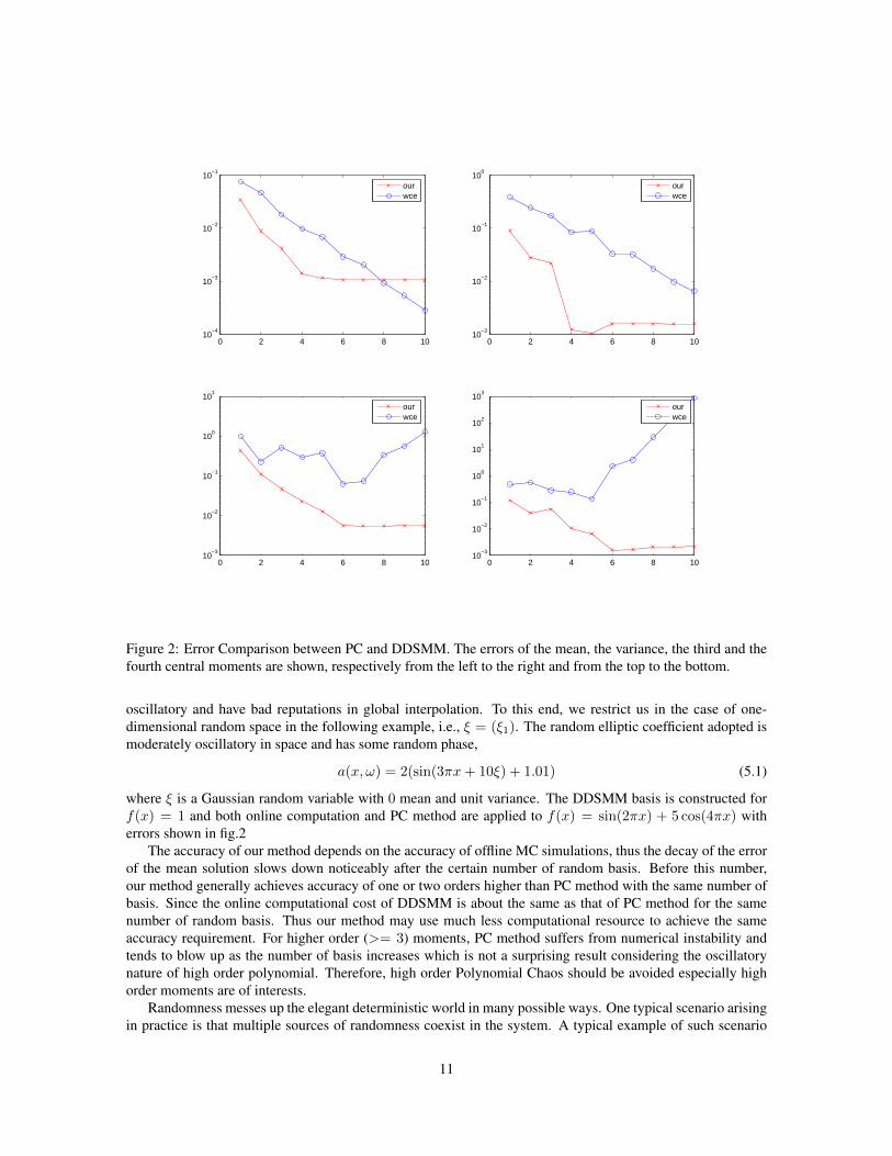
Figure 2: Error Comparison between PC and DDSMM. The errors of the mean, the variance, the third and thefourth central moments are shown, respectively from the left to the right and from the top to the bottom.

oscillatory and have bad reputations in global interpolation. To this end, we restrict us in the case of one-dimensional random space in the following example, i.e., ξ = (ξ1). The random elliptic coefficient adopted ismoderately oscillatory in space and has some random phase,

a(x, ω) = 2(sin(3πx+ 10ξ) + 1.01) (5.1)

where ξ is a Gaussian random variable with 0 mean and unit variance. The DDSMM basis is constructed forf(x) = 1 and both online computation and PC method are applied to f(x) = sin(2πx) + 5 cos(4πx) witherrors shown in fig.2

The accuracy of our method depends on the accuracy of offline MC simulations, thus the decay of the errorof the mean solution slows down noticeably after the certain number of random basis. Before this number,our method generally achieves accuracy of one or two orders higher than PC method with the same number ofbasis. Since the online computational cost of DDSMM is about the same as that of PC method for the samenumber of random basis. Thus our method may use much less computational resource to achieve the sameaccuracy requirement. For higher order (>= 3) moments, PC method suffers from numerical instability andtends to blow up as the number of basis increases which is not a surprising result considering the oscillatorynature of high order polynomial. Therefore, high order Polynomial Chaos should be avoided especially highorder moments are of interests.

Randomness messes up the elegant deterministic world in many possible ways. One typical scenario arisingin practice is that multiple sources of randomness coexist in the system. A typical example of such scenario

11

0 0.2 0.4 0.6 0.8 1−0.7

−0.6

−0.5

−0.4

−0.3

−0.2

−0.1

0

0.1

0.2

0 0.2 0.4 0.6 0.8 10

0.05

0.1

0.15

0.2

0.25

0.3

0.35

0 0.2 0.4 0.6 0.8 1−0.5

−0.4

−0.3

−0.2

−0.1

0

0.1

0.2

0 0.2 0.4 0.6 0.8 10

0.1

0.2

0.3

0.4

0.5

0.6

0.7

Exact4 Mode6 Mode9 Mode

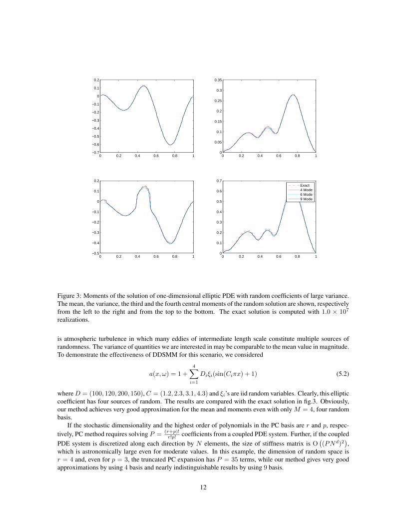
Figure 3: Moments of the solution of one-dimensional elliptic PDE with random coefficients of large variance.The mean, the variance, the third and the fourth central moments of the random solution are shown, respectivelyfrom the left to the right and from the top to the bottom. The exact solution is computed with 1.0 × 107

realizations.

is atmospheric turbulence in which many eddies of intermediate length scale constitute multiple sources ofrandomness. The variance of quantities we are interested in may be comparable to the mean value in magnitude.To demonstrate the effectiveness of DDSMM for this scenario, we considered

a(x, ω) = 1 +

4∑ı=1

Diξi(sin(Ciπx) + 1) (5.2)

whereD = (100, 120, 200, 150),C = (1.2, 2.3, 3.1, 4.3) and ξi’s are iid random variables. Clearly, this ellipticcoefficient has four sources of random. The results are compared with the exact solution in fig.3. Obviously,our method achieves very good approximation for the mean and moments even with only M = 4, four randombasis.

If the stochastic dimensionality and the highest order of polynomials in the PC basis are r and p, respec-tively, PC method requires solving P = (r+p)!

r!p! coefficients from a coupled PDE system. Further, if the coupledPDE system is discretized along each direction by N elements, the size of stiffness matrix is O

((PNd)2

),

which is astronomically large even for moderate values. In this example, the dimension of random space isr = 4 and, even for p = 3, the truncated PC expansion has P = 35 terms, while our method gives very goodapproximations by using 4 basis and nearly indistinguishable results by using 9 basis.

12

0 0.1 0.2 0.3 0.4 0.5 0.6 0.7 0.8 0.9 10

0.5

1

1.5

2

2.5

3

3.5

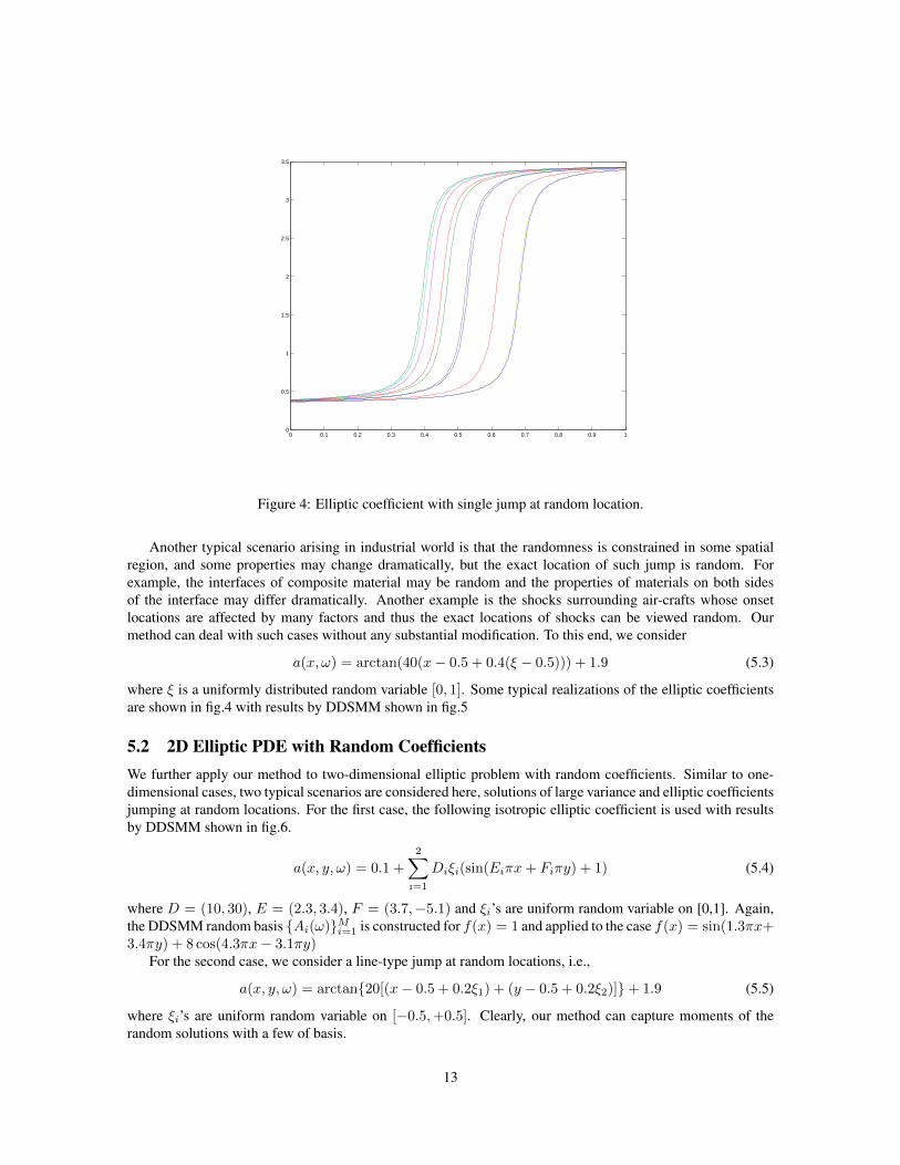
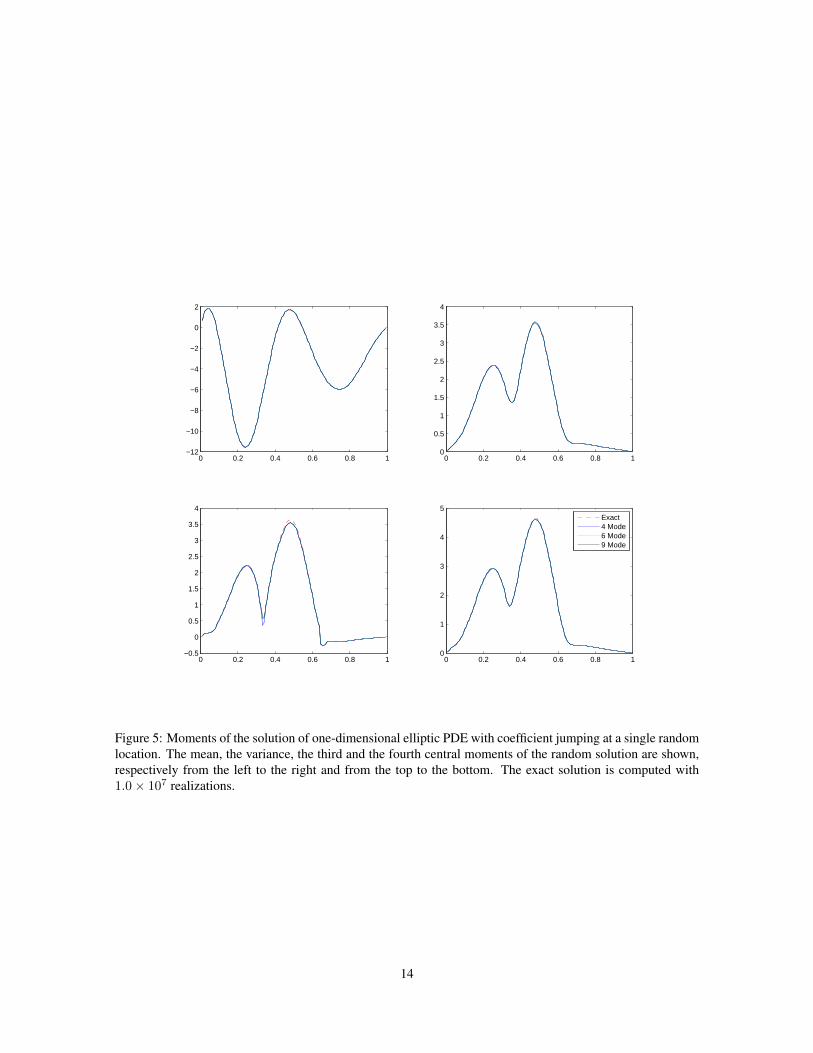
Figure 4: Elliptic coefficient with single jump at random location.

Another typical scenario arising in industrial world is that the randomness is constrained in some spatialregion, and some properties may change dramatically, but the exact location of such jump is random. Forexample, the interfaces of composite material may be random and the properties of materials on both sidesof the interface may differ dramatically. Another example is the shocks surrounding air-crafts whose onsetlocations are affected by many factors and thus the exact locations of shocks can be viewed random. Ourmethod can deal with such cases without any substantial modification. To this end, we consider

a(x, ω) = arctan(40(x− 0.5 + 0.4(ξ − 0.5))) + 1.9 (5.3)

where ξ is a uniformly distributed random variable [0, 1]. Some typical realizations of the elliptic coefficientsare shown in fig.4 with results by DDSMM shown in fig.5

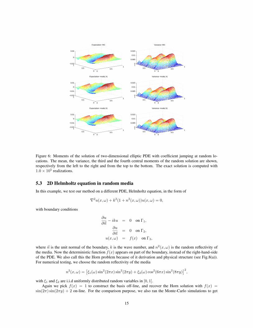
5.2 2D Elliptic PDE with Random CoefficientsWe further apply our method to two-dimensional elliptic problem with random coefficients. Similar to one-dimensional cases, two typical scenarios are considered here, solutions of large variance and elliptic coefficientsjumping at random locations. For the first case, the following isotropic elliptic coefficient is used with resultsby DDSMM shown in fig.6.

a(x, y, ω) = 0.1 +

2∑ı=1

Diξi(sin(Eiπx+ Fiπy) + 1) (5.4)

where D = (10, 30), E = (2.3, 3.4), F = (3.7,−5.1) and ξi’s are uniform random variable on [0,1]. Again,the DDSMM random basis Ai(ω)Mi=1 is constructed for f(x) = 1 and applied to the case f(x) = sin(1.3πx+3.4πy) + 8 cos(4.3πx− 3.1πy)

For the second case, we consider a line-type jump at random locations, i.e.,

a(x, y, ω) = arctan20[(x− 0.5 + 0.2ξ1) + (y − 0.5 + 0.2ξ2)]+ 1.9 (5.5)

where ξi’s are uniform random variable on [−0.5,+0.5]. Clearly, our method can capture moments of therandom solutions with a few of basis.

13

0 0.2 0.4 0.6 0.8 1−12

−10

−8

−6

−4

−2

0

2

0 0.2 0.4 0.6 0.8 10

0.5

1

1.5

2

2.5

3

3.5

4

0 0.2 0.4 0.6 0.8 1−0.5

0

0.5

1

1.5

2

2.5

3

3.5

4

0 0.2 0.4 0.6 0.8 10

1

2

3

4

5

Exact4 Mode6 Mode9 Mode

Figure 5: Moments of the solution of one-dimensional elliptic PDE with coefficient jumping at a single randomlocation. The mean, the variance, the third and the fourth central moments of the random solution are shown,respectively from the left to the right and from the top to the bottom. The exact solution is computed with1.0× 107 realizations.

14

00.5

1

0

0.5

1−0.02

0

0.02

Expectation−MC

00.5

1

0

0.5

10

0.005

0.01

0.015

Variance−MC

00.5

1

0

0.5

1−0.02

−0.01

0

0.01

Expectation−mode( 4)

00.5

1

0

0.5

10

0.005

0.01

0.015

Variance−mode( 4)

00.5

1

0

0.5

1−0.02

−0.01

0

0.01

Expectation−mode( 6)

00.5

1

0

0.5

10

0.005

0.01

0.015

Variance−mode( 6)

Figure 6: Moments of the solution of two-dimensional elliptic PDE with coefficient jumping at random lo-cations. The mean, the variance, the third and the fourth central moments of the random solution are shown,respectively from the left to the right and from the top to the bottom. The exact solution is computed with1.0× 105 realizations.

5.3 2D Helmholtz equation in random mediaIn this example, we test our method on a different PDE, Helmholtz equation, in the form of

∇2u(x, ω) + k2(1 + n2(x, ω))u(x, ω) = 0,

with boundary conditions

∂u

∂~n− iku = 0 on Γ1,

∂u

∂~n= 0 on Γ2,

u(x, ω) = f(x) on Γ3,

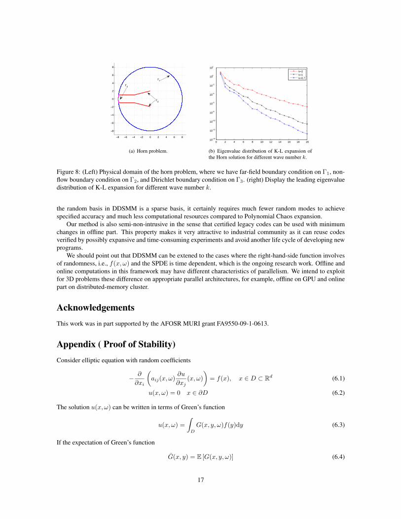
where ~n is the unit normal of the boundary, k is the wave number, and n2(x, ω) is the random reflectivity ofthe media. Now the deterministic function f(x) appears on part of the boundary, instead of the right-hand-sideof the PDE. We also call this the Horn problem because of it derivation and physical structure (see Fig.8(a)).For numerical testing, we choose the random reflectivity of the media

n2(x, ω) =[ξ1(ω) sin2(2πx) sin2(2πy) + ξ2(ω) cos2(6πx) sin2(8πy)

]2,

with ξ1 and ξ2 are i.i.d uniformly distributed random variables in [0, 1].Again we pick f(x) = 1 to construct the basis off-line, and recover the Horn solution with f(x) =

sin(2π) sin(2πy) + 2 on-line. For the comparison purpose, we also ran the Monte-Carlo simulations to get

15

00.5

1

0

0.5

1−0.2

0

0.2

Expectation−MC

00.5

1

0

0.5

10

0.01

0.02

0.03

Variance−MC

00.5

1

0

0.5

1−0.2

0

0.2

Expectation−mode( 4)

00.5

1

0

0.5

10

0.01

0.02

0.03

Variance−mode( 4)

00.5

1

0

0.5

1−0.2

0

0.2

Expectation−mode( 6)

00.5

1

0

0.5

10

0.01

0.02

0.03

Variance−mode( 6)

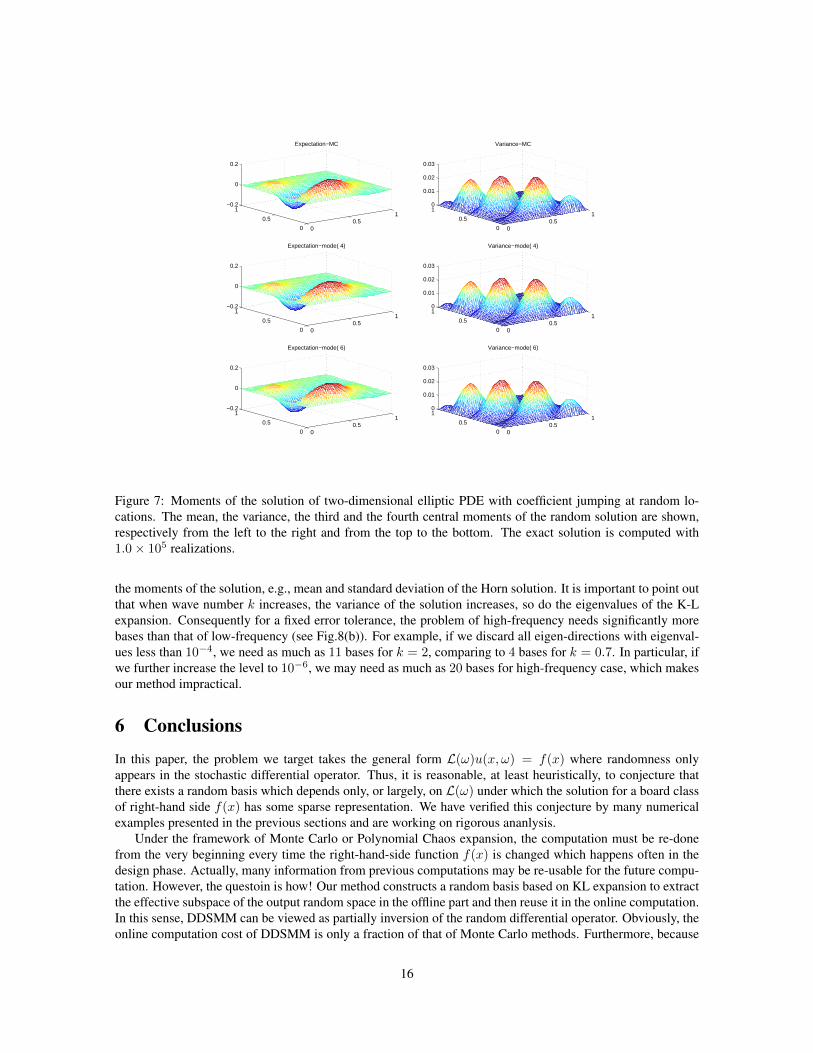
Figure 7: Moments of the solution of two-dimensional elliptic PDE with coefficient jumping at random lo-cations. The mean, the variance, the third and the fourth central moments of the random solution are shown,respectively from the left to the right and from the top to the bottom. The exact solution is computed with1.0× 105 realizations.

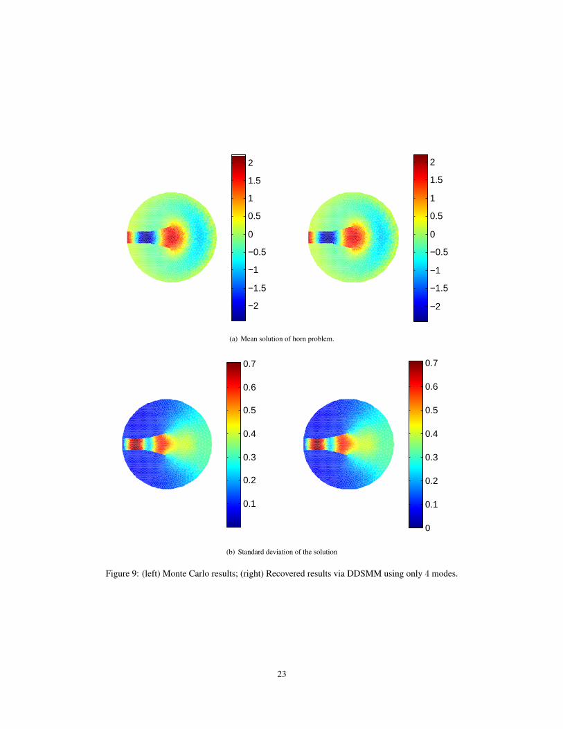
the moments of the solution, e.g., mean and standard deviation of the Horn solution. It is important to point outthat when wave number k increases, the variance of the solution increases, so do the eigenvalues of the K-Lexpansion. Consequently for a fixed error tolerance, the problem of high-frequency needs significantly morebases than that of low-frequency (see Fig.8(b)). For example, if we discard all eigen-directions with eigenval-ues less than 10−4, we need as much as 11 bases for k = 2, comparing to 4 bases for k = 0.7. In particular, ifwe further increase the level to 10−6, we may need as much as 20 bases for high-frequency case, which makesour method impractical.

6 Conclusions

In this paper, the problem we target takes the general form L(ω)u(x, ω) = f(x) where randomness onlyappears in the stochastic differential operator. Thus, it is reasonable, at least heuristically, to conjecture thatthere exists a random basis which depends only, or largely, on L(ω) under which the solution for a board classof right-hand side f(x) has some sparse representation. We have verified this conjecture by many numericalexamples presented in the previous sections and are working on rigorous ananlysis.

Under the framework of Monte Carlo or Polynomial Chaos expansion, the computation must be re-donefrom the very beginning every time the right-hand-side function f(x) is changed which happens often in thedesign phase. Actually, many information from previous computations may be re-usable for the future compu-tation. However, the questoin is how! Our method constructs a random basis based on KL expansion to extractthe effective subspace of the output random space in the offline part and then reuse it in the online computation.In this sense, DDSMM can be viewed as partially inversion of the random differential operator. Obviously, theonline computation cost of DDSMM is only a fraction of that of Monte Carlo methods. Furthermore, because

16

8 6 4 2 0 2 4 6 8

8

6

4

2

0

2

4

6

8

1

3

2

(a) Horn problem.

0 2 4 6 8 10 12 14 16 18 2010−14

10−12

10−10

10−8

10−6

10−4

10−2

100

102

k=2k=1k=0.7

(b) Eigenvalue distribution of K-L expansion ofthe Horn solution for different wave number k.

Figure 8: (Left) Physical domain of the horn problem, where we have far-field boundary condition on Γ1, non-flow boundary condition on Γ2, and Dirichlet boundary condition on Γ3. (right) Display the leading eigenvaluedistribution of K-L expansion for different wave number k.

the random basis in DDSMM is a sparse basis, it certainly requires much fewer random modes to achievespecified accuracy and much less computational resources compared to Polynomial Chaos expansion.

Our method is also semi-non-intrusive in the sense that certified legacy codes can be used with minimumchanges in offline part. This property makes it very attractive to industrial community as it can reuse codesverified by possibly expansive and time-consuming experiments and avoid another life cycle of developing newprograms.

We should point out that DDSMM can be extened to the cases where the right-hand-side function involvesof randomness, i.e., f(x, ω) and the SPDE is time dependent, which is the ongoing research work. Offline andonline computations in this framework may have different characteristics of parallelism. We intend to exploitfor 3D problems these difference on appropriate parallel architectures, for example, offline on GPU and onlinepart on distributed-memory cluster.

AcknowledgementsThis work was in part supported by the AFOSR MURI grant FA9550-09-1-0613.

Appendix ( Proof of Stability)Consider elliptic equation with random coefficients

− ∂

∂xi

(aij(x, ω)

∂u

∂xj(x, ω)

)= f(x), x ∈ D ⊂ Rd (6.1)

u(x, ω) = 0 x ∈ ∂D (6.2)

The solution u(x, ω) can be written in terms of Green’s function

u(x, ω) =

∫D

G(x, y, ω)f(y)dy (6.3)

If the expectation of Green’s function

G(x, y) = E [G(x, y, ω)] (6.4)

17

exists and the covariance function

CovG(x, y, x′, y′) = E[(G(x, y, ω)− G(x, y))(G(x′, y′, ω)− G(x′, y′))

](6.5)

exists and continuous, Green’s function G(x, y, ω) has KL expansion

G(x, y, ω) = G(x, y) +

∞∑i=1

√λiGi(x, y)Bi(ω) (6.6)

where λi, Gi(x, y)∞i=1 are eigenpaires of covariance function CovG(x, y, x′, y′)∫D×D

CovG(x, y, x′, y′)Gi(x′, y′)dx′dy′ = λiGi(x, y) (6.7)

with orthogonality conditions ∫D×D

Gi(x, y)Gj(x, y)dxdy = δij (6.8)

E [Bi(ω)Bj(ω)] = δij (6.9)

andBi(ω) =

1√λi

∫D×D

(G(x, y, ω)− G(x, y)

)Gi(x, y)dxdy (6.10)

Then the solution u(x, ω) can be written as

u(x, ω) =

∞∑i=0

√λiFi(x)Bi(ω) (6.11)

whereFi(x) =

∫D

Gi(x, y)f(y)dy (6.12)

Lemma 6.1. ‖Fi(x)‖2 ≤ ‖f(x)‖2

Proof. For each x,

|Fi(x)|2 = |∫D

Gi(x, y)f(y)dy|2

≤∫D

Gi(x, y)2dy

∫D

f2(y)dy

=

∫D

Gi(x, y)2dy‖f(y)‖22

Integrate on both sides

‖Fi(x)‖22 =

∫D

F 2i (x)dx

≤∫D

∫D

Gi(x, y)2dydx‖f(y)‖22

= ‖f(y)‖22

The orthogonality of Gi is used in the last equality.

18

Now consider KL expansion of u(x, ω)

u(x, ω) = u(x) +

∞∑i=1

√θiφi(x)Ai(ω) (6.13)

where √θi, φi(x)∞i=1 are eigenpaires of the covariance function Covu(x, y), i.e.,∫

D

Covu(x, y)φi(y)dy = θiφi(x) (6.14)

andAi(ω) =

1√θi

∫D

u(x, ω)φ(x)dx (6.15)

with bi-orthogonality ∫D

φi(x)φj(x)dx = δij

E [Ai(ω)Aj(ω)] = δij

Combine eqn.6.11 and eqn.6.13, we have

∞∑j=1

√λjFj(x)Bj(ω) =

∞∑j=1

√θjφj(x)Aj(ω)

in which the mean u(x) has been cancelled on both sides. Multiple both sides by Fi(x) and integrate over D,

∞∑j=1

αij√λjBj(ω) =

∞∑j=1

βij√θjAj(ω) (6.16)

where

αij =

∫D

Fi(x)Fj(x)dx

βij =

∫D

Fi(x)φj(x)dx

The equality can be written in matrix form(α11 α12

α21 α22

)(Λ

121 0

0 Λ122

)(B1

B2

)=

(β11 β12

β21 β22

)(Θ

121 0

0 Θ122

)(A1

A2

)(6.17)

whereα11 ∈ RN1×N1 , Λ1 = diag (λ1, . . . , λN1), Λ2 = diag (λN1+1, . . . ), β11 ∈ RN1×N2 , Θ1 = diag (θ1, . . . , θN2

),Θ2 = diag (θN2+1, . . . ), B1 ∈ RN1 and A1 ∈ RN2 . or

α11Λ121 B1 + α12Λ

122 B2 = β11Θ

121 A1 + β12Θ

122 A2 (6.18)

α21Λ121 B1 + α22Λ

122 B2 = β21Θ

121 A1 + β22Θ

122 A2 (6.19)

Before proceeding to the error analysis, we have the following bounds

Lemma 6.2.

|αij | ≤ ‖Fi(x)‖2‖Fj(x)‖2 ≤ ‖f(x)‖22|βij | ≤ ‖Fi(x)‖2 ≤ ‖f(x)‖2

19

Suppose we can construct Ai(ω)N2i=1 exactly without numerical errors in offline computation and apply

this basis to the case with right hand side function g(x) ∈ L2(D). By solving the coupled equations resultingfrom Galerkin projection, we have the numerical solution

v(x, ω) =

N2∑i=0

vi(x)Ai(ω) (6.20)

The solution can be written in terms of Green’s function

v(x, ω) =

∞∑i=0

√λiHi(x)Bi(ω) (6.21)

whereHi(x) =

∫D

Gi(x, y)g(y)dy. (6.22)

By Lemma (6.1), it is clear that ‖Hi(x)‖2 ≤ ‖g(x)‖2. In addition, the expansion of v(x, ω) on the basis Ai(ω)is

v(x, ω) =

∞∑i=0

vi(x)Ai(ω). (6.23)

Thus the error is

E(x, ω) = v(x, ω)− v(x, ω)

= EA(x, ω) + EB(x, ω),

where

EA(x, ω) =

N2∑i=0

[vi(x)− v(x)]Ai(ω), (6.24)

EB(x, ω) =

∞∑i=1

√λiHi(x)Bi(ω)−

N2∑i=1

vi(x)Ai(ω). (6.25)

The first error is due to Galerkin projection, and the second is due to approximation of Bi by Ai. Forsimplicity, we assume ‖g(x)‖2 = 1. To bound the second error term, we recall

vj(x) = E [v(x, ω)Aj(ω)] =

∞∑i=1

√λiHi(x)E [Bi(ω)Aj(ω)] , (6.26)

and plug it into EB(x, ω). We have, after changing the order of summation,

EB(x, ω) = EB1(x, ω) + EB2(x, ω), (6.27)

and

EB1(x, ω) =

N1∑i=1

√λiHi(x)

Bi(ω)−N2∑j=1

E [Bi(ω)Aj(ω)]Aj(ω)

,

EB2(x, ω) =

∞∑i=N1+1

√λiHi(x)

Bi(ω)−N2∑j=1

E [Bi(ω)Aj(ω)]Aj(ω)

.

20

Theorem 6.3. Given the condition that N1 satisfies

∞∑i=N1+1

√λi ≤ ε,

there exists N2, such that for ∀N2 ≥ N2, we have

E[∫|EB(x, ω)|2dx

]≤ 2ε2.

Proof. Proof is given by the following inequality

E[∫|EB(x, ω)|2dx

]≤ E

[∫|EB1(x, ω)|2dx

]+ E

[∫|EB1(x, ω)|2dx

],

and Lemma (6.4), (6.5).

Lemma 6.4. Given the condition that N1 satisfies

∞∑i=N1+1

√λi ≤ ε,

we have

E[∫|EB1(x, ω)|2dx

]≤ ε2.

Proof. (Lemma 6.4) Based on Cauchy-Schwarz inequality, we have

E[∫|EB1(x, ω)|2dx

]= E

∫ | ∞∑i=N1+1

√λiHi(x)

Bi(ω)−N2∑j=1

E [Bi(ω)Aj(ω)]Aj(ω)

|2dx

≤∞∑

i=N1+1

√λi

∫|Hi(x)|2dx ·

∞∑i=N1+1

√λiE

[|Bi(ω)−

∑E [Bi(ω)Aj(ω)]Aj(ω)|

]2≤ (

∞∑i=N1+1

√λi)

2.

The last inequality is given by

‖Hi(x)‖2 ≤ ‖g(x)‖2 = 1,

and

E[|Bi(ω)−

∑E [Bi(ω)Aj(ω)]Aj(ω)|

]2= 1−

N2∑j=1

(E [Bi(ω)Aj(ω)])2 ≤ 1.

Lemma 6.5. For a fixed N1, there exists a large N2 such that N2 ≥ N2 we have

E[∫|EB2(x, ω)|2dx

]≤ ε.

21

Proof. (Lemma 6.5) Now apply Cauchy-Schwarz inequality again on the error term EB2(x, ω) and we have

E[∫|EB2(x, ω)|2dx

]= E

∫ | N1∑i=1

√λiHi(x)

Bi(ω)−N2∑j=1

E [Bi(ω)Aj(ω)]Aj(ω)

|2dx

≤N1∑i=1

∫|Hi(x)|2dx ·

N1∑i=1

λiE[|Bi(ω −

∑E [Bi(ω)Aj(ω)]Aj(ω))|

]2≤ N1 ·

N1∑i=1

λi

(1−

N2∑j=1

(E [Bi(ω)Aj(ω)])2).

Since Aii=1,... is a complete orthonormal basis of the space L2(Ω), for any normalized random variableB(ω) we have

limN2→∞

N2∑j=1

(E [B(ω)Aj(ω)])2 = 1.

Hence there exists integer N (i), such that

N(i)∑j=1

(E [Bi(ω)Aj(ω)])2 ≥ 1−min(1,ε2

N21λi

).

Now we chooseN2 ≥ N2 = max

i=1,...,N1

N (i),

and have

E[∫|EB2(x, ω)|2dx

]≤ N1 ·

N1∑i=1

λi

(1−

N2∑j=1

(E [Bi(ω)Aj(ω)])2)

≤ N1 ·N1∑i=1

λi

(1− (1−min(1,

ε2

N21λi

)))

≤ ε2

22

−2

−1.5

−1

−0.5

0

0.5

1

1.5

2

−2

−1.5

−1

−0.5

0

0.5

1

1.5

2

(a) Mean solution of horn problem.

0.1

0.2

0.3

0.4

0.5

0.6

0.7

0

0.1

0.2

0.3

0.4

0.5

0.6

0.7

(b) Standard deviation of the solution

Figure 9: (left) Monte Carlo results; (right) Recovered results via DDSMM using only 4 modes.

23

2

4

6

8

10

12

14

16

18x 10−3

2

4

6

8

10

12

14

16

18

x 10−3

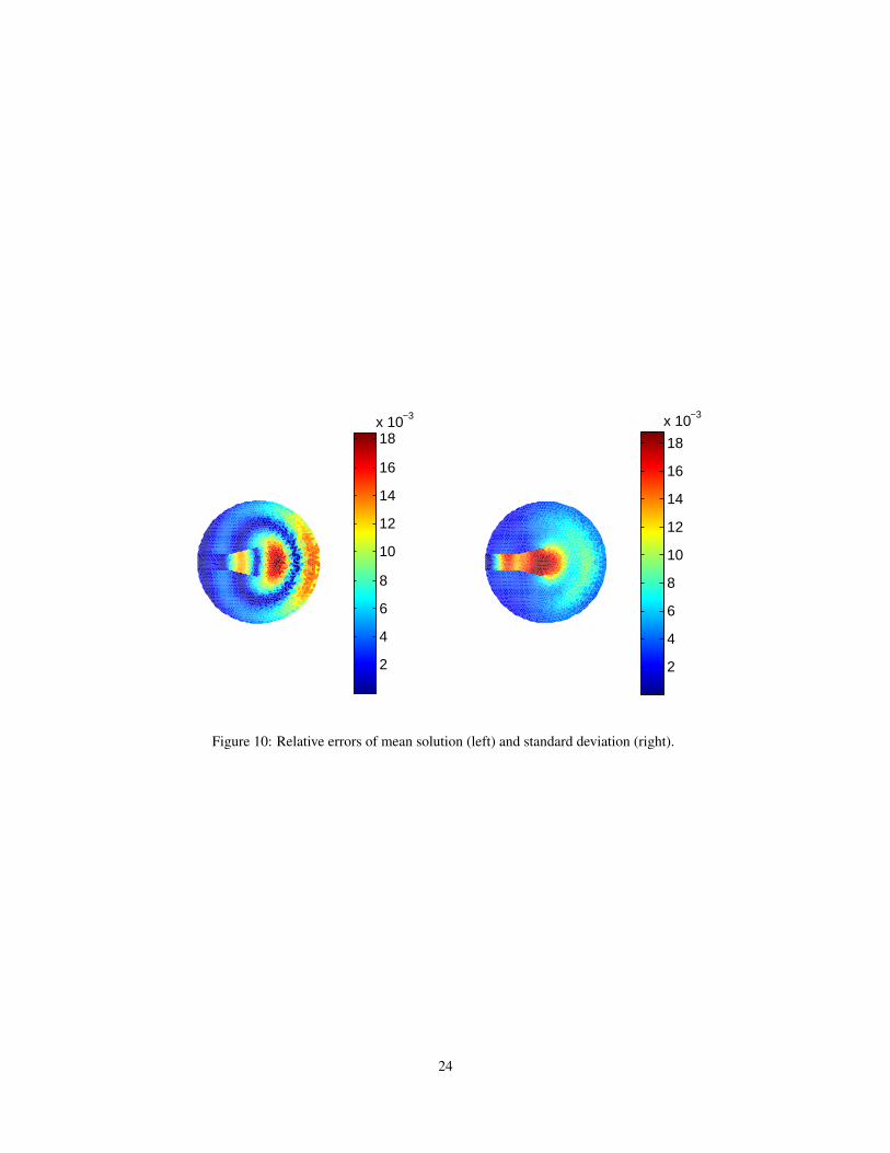
Figure 10: Relative errors of mean solution (left) and standard deviation (right).

24