› ~daddel › MATH22AL › LABS › LAB7 › ... · MATH 22AL Lab # 7 1Objectives2019-05-29 · MATH 22AL Lab # 7 1Objectives ... { In Computer LAB (2118 MSB) click on terminal

MATH 22ALLab # 7

1 Objectives

In this LAB you will explore the following topics using MATLAB.

• What to do with Inconsistent Linear System

• Minimizing the error in solving Inconsistent Linear system

• Orthogonal Projections.

• Least square solution.

• Normal Equation

• Polynomial Interpolation.

2 What to turn in for this lab

Please save and submit your MATLAB session.

Important: Do not Change the name of the Variables that you supposed to type in MATLAB, type

as you are asked.

1

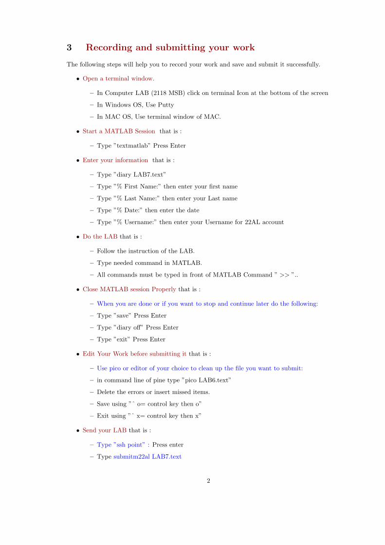
3 Recording and submitting your work

The following steps will help you to record your work and save and submit it successfully.

• Open a terminal window.

– In Computer LAB (2118 MSB) click on terminal Icon at the bottom of the screen

– In Windows OS, Use Putty

– In MAC OS, Use terminal window of MAC.

• Start a MATLAB Session that is :

– Type ”textmatlab” Press Enter

• Enter your information that is :

– Type ”diary LAB7.text”

– Type ”% First Name:” then enter your first name

– Type ”% Last Name:” then enter your Last name

– Type ”% Date:” then enter the date

– Type ”% Username:” then enter your Username for 22AL account

• Do the LAB that is :

– Follow the instruction of the LAB.

– Type needed command in MATLAB.

– All commands must be typed in front of MATLAB Command ” >> ”..

• Close MATLAB session Properly that is :

– When you are done or if you want to stop and continue later do the following:

– Type ”save” Press Enter

– Type ”diary off” Press Enter

– Type ”exit” Press Enter

• Edit Your Work before submitting it that is :

– Use pico or editor of your choice to clean up the file you want to submit:

– in command line of pine type ”pico LAB6.text”

– Delete the errors or insert missed items.

– Save using ”ˆ o= control key then o”

– Exit using ”ˆ x= control key then x”

• Send your LAB that is :

– Type ”ssh point” : Press enter

– Type submitm22al LAB7.text

2

4 Background, Reading Part : Introduction

Probably you know how to construct a curve through specified points. For example how to construct

a line passing through two given points, or a parabola passing through three points. In general you

can construct a polynomial of degree n that passes through n+ 1 specified points. Such a polynomial

is called Interpolating polynomial.

What happens if you have for example more than two points and you want to represent your data

with a straight line? In cases like this we face an inconsistent system of linear equations Ax = b.

Instead of solving Ax = b we try to find an x such that Ax is good approximation of b.

3

5 Background, Reading Part : Origin of inconsistent sys-tems?

Inconsistent systems arise often in applications. Scientists try to find a functional relationship be-

tween variables. They collect data, which usually involve experimental error and by studying this data

or from other findings, they suggest a mathematical model for it, “functional relationship between

variables.”

Because of measurement error, usually a polynomial that passes through all the given points is not the

a true representation of the relationship between variable. A lower degree polynomial may represent

the relationship better. To find coefficients of such polynomial the method introduced in LAB 5

is useful. But most of the times this method gives us an inconsistent system, which requires an

approximation. In this laboratory we discuss such approximation, called “Least Square Solution”.

4

5.1 Background, Reading Part : Example 1

Suppose that you know two variables x and y have linear relationship that is y = mx+ c. Suppose in

an experiment you obtained the following data:

x1 = 52 y1 = 2

x2 = 3 y2 = 92

x3 = 32 y3 = 2

x4 = 1 y4 = 1

If you want to fit a line with equation y = mx+ b through these points. As you learned in Laboratory

5, you need to form the following system of linear equations.

52m + b = 23m + b = 9

232m + b = 21m + b = 1

This is an overdetermined system. That is it has more equation than unknowns. Over determined

systems usually are inconsistent.

Writing the matrix equation for this linear system we get52 13 132 11 1

[ mb

]=

29221

Find the reduced row echelon form of the augmented matrix.

52 1 | 23 1 | 9

232 1 | 21 1 | 1

=⇒

1 0 | 00 1 | 00 0 | 10 0 | 0

As you see the rank of rref of the augmented matrix is 3 while the rank of the coefficient matrix is 2.

Therefore the system is inconsistent. So there is no x such that Ax = b or Ax− b = 0.

Since Ax − b is non-zero how about forcing it to be as small as possible. So, the goal is to find an

approximation, Ax, for b or to minimize d = Ax− b?

Restating the question:

How could we find an x such that Ax is as close as possible to b?

5

6 Background, Reading Part : Minimizing Ax-b

Let A be an m×n matrix. Suppose that Ax = b is an inconsistent system, we are interested in finding

an x such that Ax is as close as possible to b.

Lets first look at the Example 1. There are several ways to make your line “close” to given points,

depending how we define “closeness”. Usual way is to add the square of d1, d2d3. . . dn, then minimize

the sum of squares. See figure bellow.

This method is called “ least square Approximation ”.

We may also think that Ax in a m × 1 vector and b is another m × 1 vector. We want to minimize

Ax − b. Assume that our vector space is an Inner Product Space with the usual Euclidean inner

product, minimizing (Ax− b) translates to minimizing the distance ||Ax− b|| between the two vectors

Ax and b. Note that ||Ax− b|| is the length of the vector Ax− b.

One thing which helps understanding the procedure of minimizing the distance between Ax and b is

the fact that Ax is a vector in column space of A. (Why?)

Since Ax = b is not consistent, b is not in the column space of A. So we are looking for a vector,

Ax, in the column space of A which is closest to the vector b. It can be proved ( see your text book)

that such a vector is the orthogonal projection of b onto the column space of A. Now if Ax is the

orthogonal projection of b onto col(A) then Ax− b is orthogonal to col(A). (why?) That is Ax− b is

in null(At) . So

At(b−Ax) = 0

or

AtAx = Atb.

This system of linear equations is consistent ( Why?) and it is called Normal System. Moreover

if the column of A are linearly independent, then AtA is invertible and

x = (AtA)−1(At)b

6

is the unique solution of the system AtAx = Atb.

If columns of A are orthonormal then AtA = I and we can easily compute x = Atb, and the closest

vector p in the column space of A to b is p = AAtb.

7

6.1 Background, Reading Part : Orthogonal projection of b onto W

Let b be a vector in Rm and W be a subspace of Rm spanned by the vectors

w1, w2, w3, . . . wn

. To find orthogonal projection of b onto W denoted by ProjW b form a matrix A whose columns are

the vectors

w1, w2, w3, . . . wn

then solve the normal system

AtAx = Atb.

The solution vector x is the orthogonal projection of b onto W . Orthogonal Projection of Rm onto

W

Let W be a subspace of Rm spanned by the basis vectors

w1, w2, w3, . . . wn.

To find orthogonal projection of Rm onto W denoted by [P ] form a matrix A whose columns are the

vectors

w1, w2, w3, . . . wn

then transformation

P = A(AtA)−1At

is called the orthogonal projection of Rm onto W .

8

7 Background, Reading Part : Least Square Lines

Assume that y is a linear function of x that is y = mx+b and experimental data (x1, y1), (x2, y2), . . . , (xn, yn)

is given. We want to find the parameters m and b such that the line y = mx + b be as “ close ” as

possible to the given points.

Set x =

[mb

]A =

x1 1x2 1...

...xn 1

b =

y1y2...yn

solve the linear system AtAx = Atb.

9

Start Typing in MATLAB

7.1 Example 2

Find the equation y = mx + c of the least square line that best fits the data from Example1:

x1 = 52 y1 = 2

x2 = 3 y2 = 92

x3 = 32 y3 = 2

x4 = 1 y4 = 1

Note: This line is called least-squares line and the coefficients m and c are called regression

coefficients.

Solution :

Steps : First form your matrix A, then solve the linear system AtAx = Atb.

i) Enter the data matrix D as:

Type :

D = [5/2 3 3/2 1; 1 1 1 1 ; 2 9/2 2 1 ]′

Type :

A = D(:, [1 2])

Type :

b = D(:, 3)

ii) Find the augmented matrix of the system AtAx = Atb

Type :

AG = [A′ ∗A A′ ∗ b]

Then find the rref of the augmented matrix

Type :

RRAG = rref(AG)

This should give you m = 7/5 and c = −17/40

10

8 Example 3

Find equation of a polynomial of degree 3, y = a3x3 + a2x2 + a1x + a0 that best fits the following

data.

x1 = 2 y1 = 7x2 = 1 y2 = −2x3 = 0 y3 = −7x4 = −2 y4 = −27x5 = 5 y4 = 110x6 = −1 y4 = −20

Solution :

Note: The method used to fit a straight line to data points in Example 1 can be easily generalized

to a polynomial of a given degree

By plugging the given six points in the equation of the polynomial, we get a system of six linear

equations. By solving this linear system we find the coefficients of the third degree polynomial

y = a3x3 + a2x

2 + a1x + a0.

The linear system Ax = b would bex31 x2

1 x1 1x32 x2

2 x2 1x33 x2

3 x3 1x34 x2

4 x4 1x35 x2

5 x5 1x36 x2

6 x6 1

a3a2a1a0

=

y1y2y3y4y5y6

Steps : First form your matrix A, then solve the linear system AtAx = Atb.

To distinguish matrices of this example with the previous ones we call the coefficient matrix A1.

To form your matrix A1

Type :

D = [2 1 0 − 2 5 − 1; 1 1 1 1 1 1; 7 − 2 − 7 − 27 110 − 20]′

Type :

A1 = [D(:, 1).̂ 3 D(:, 1).̂ 2 D(:, 1) D(:, 2)]

Note : D(:, 1).̂ 3 has two parts:

• D(:, 1) Choosing the first column of D

• .̂ 3 raising each entry to the third power

To enter your matrix b

11

Type :

b1 = D(:, 3)

Solve the linear system (A1)t(A1)x = (A1)t(b1)

First form the augmented matrix

Type :

AG1 = [(A1)′ ∗ (A1) (A1)′ ∗ b1]

Then find the rref of the augmented matrix:

Type :

RRAG1 = rref(AG1)

This should give you

a3 = 252/347,

a2 = −21/233,

a1 = 2439/394,

a0 = −3301/344.

12

9 Exercise:

1. Enter matrices A2 and b2 by typing

Type :

A2 = [1 2 3; 4 5 6; 7 8 9; 3 2 4; 6 5 4; 9 8 7]

b2 = [1 1 1 1 1 1]′

a.) Show that (A2)x = b2 is inconsistent. Show this in two ways:

a1.) By finding

Type :

RRA2 = rref([A2 b2])

and

a2.) Finding both

Type :

rankA2b = rank([A2 b2])

and

Type :

rankA2 = rank(A2)

13

Problem 1 continues:

b.) Show that the system (A2)t(A2)x = (A2)tb2 is a consistent system and find a solution

for (A2)t(A2)x = (A2)tb2.

Type :

N1A2 = [A2′ ? A2 A2′ ? b2]

Type :

RRN1A2 = rref(N1A2)

To get the solution

Type :

X2 = RRN1A2(:, 4)

c.) Find ||A2 ? X2− b2|| the norm of the vector A2 ? X2− b2 by typing norm(A2 ? X2− b2)

where X2 is your solution from part (b).

Type :

E2 = A2 ? X2− b2

Type :

NOR2 = norm(E2)

i) Find a random vector, say Z2 , in the column space of A2 by typing

Type :

Z2 = A2 ∗ [1 2 − 1]′

ii) Compute ||Z2− b2|| by typing

Type :

NORZ2 = norm(Z2− b2)

Compare this value with ||A2 ? X2− b2|| which one is smaller?

Type :

% NORZ2 is smaller than NOR2

or Type :

% NORZ2 is larger than NOR2

14


iii) Find two other vectors, Z3, and Z4, in column space of A2 as we found Z2 in part(ii),

Type :

Z3 = A2 ? (10 ? rand(3, 1))

Type :

Z4 = A2 ? (10 ? rand(3, 1))

Find the norm of ||Z3− b2|| and ||Z4− b2||.

Type :


Type :


Compare the results with A2 ? X2− b2.

Type :

DNORM12 = norm(Z2− b2)− norm(A2 ? X2− b2)

Type :

DNORM32 = norm(Z3− b2)− norm(A2 ? X2− b2)

No matter what vector you choose in column space of A2, the distance of that vector

from b2 will be larger than distance of A2 ? X2 from b2. Think if you can prove this

(challenging).

15


d) Is A2tA2 invertible?

You may check this by one of the following ways:

i)) Finding det(A2tA2) Note: Recall det(C) 6= 0 ⇐⇒ C is invertible

Type :

DETA2TA2 = det(A2′ ? A2)

ii)) Finding rref(AtA). Note: Recall rref(C) = I ⇐⇒ C is invertible

Type :

RRA2TA2 = rref(A2′ ? A2)

e) Are the columns of A2 linearly independent?

Type :

RREA2 = rref(A2)

Explain Enter your answer after typing %.

f) Are the rows of A2 are linearly independent?

Explain Enter your answer after typing %.

g) Find a basis for the column space of A2.

Enter your answer after typing %.

16


h) Find a basis for the row space of A2.


i) How many solutions does A2 ? x = 0 have?


j) What is the number of solutions of A2tA2 ? x = 0?


k) Find a basis for the range of the linear transformation defined by A2.

Note: TA2 is defined to be a linear transformation which maps any vector x to

A2 ? x. That is TA2 = A2 ? x. Also the range of the Linear transformation represented by

A2 is the same as the column space of A2.

l) Find a basis for the null(TA2).


m) Find nullity of A2, TA2 and A2tA2.


n) Find rank(A2), rank(A2t), rank(TA2) and rank(A2tA2).

17

2) Recall the following theorem: If B is an m×n matrix, then the following are equivalent:

i) Columns of B are linearly independent. ii) BtB is an invertible matrix.

a) Determine if the following vectors are linearly independent.

v1 = (1, 3,−2, 0, 2)

v2 = (2, 6,−5,−2, 4)

v3 = (0, 0, 5, 10, 0)

v4 = (2, 6, 0, 8, 4)

(Note: form a matrix B1 whose columns are the vectors v1, v2, v3, v4, then find det(B1tB1).

Type :

B1 = [1 3 − 2 0 2; 2 6 − 5 − 2 4; 0 0 5 10 0; 2 6 0 8 4]′

Type :

B1TB1 = B1′ ? B1

Type :

DETB1TB1 = det(B1TB1)

If B1′ ? B1 is not invertible

Type :

%B1TB1 is not invertible

If B1′ ? B1 is invertible

Type :

%INV B1TB1 = inv(B1TB1)

b) Determine if the following vectors are linearly independent.

v1 = (0, 0,−2, 0, 7, 12)

v2 = (2, 4,−10, 6, 12, 28)

v3 = (2, 4,−5, 6,−5,−1)

Repeat the steps in part(a) above:

Form a matrix B2 whose columns are the vectors v1, v2, v3, then find det(B2tB2).

Type :

B2TB2 = B2′ ? B2

Type :

DETB2TB2 = det(B2TB2)

If B2′ ? B2 is not invertible

Type :

%B2TB2 is not invertible

If B2′ ? B2 invertible

Type :

%INV B2TB2 = inv(B2TB2)

18

3. Find an equation of the line that passes through the points (3, 4) and (1, 2).

a.) Using the least square solution.

Type :

Slope1= Enter slope of the line

Intercept1= Enter the y-intercept

b.) Using the regular algebraic way: Use pen and paper.

Type :

Slope2= Enter slope of the line

Intercept2= Enter the y-intercept

19

4. Consider the following set of points:

(3, 4), (1, 2), (−1, 1), (6, 5), (7, 9). Find a polynomial of degree two y = a2x2 + a1x + a0, that

best fits the points given above.

Enter this points in a matrix :

Type :

E4 = [ 3 1 − 1 6 7; 4 2 1 5 9; 1 1 1 1 1]′

To create a matrix of x-values

Type :

X = E4(:, 1)

To create a matrix of y-values

Type :

Y = E4(:, 2)

Create a 5× 3 matrix A4

Type :

A4 = [X.̂2 X E4(:, 3)]

The first column is the x -values raised to second power.

The second column is x-values.

The Third column is ones.

Now in A4x = b the vector x is

x =

a2a1a0

and b is the vector of y-values.

Type :

b = Y

Then find the solution to the normal system A4tA4X = A4tb.

To solve this system you may find rref([A4tA4 A4tb]

Type :

RRA4AGUM = rref([A4′ ? A4 A4′ ? b])

Enter Your Answers for a2, a1 and a0 as

Type :

a2 = Your answer for a2

Type :


Type :


20

ii) Find a polynomial of degree three, y = b3x3 + b2x

2 + b1x + b0 that best fits the points

(3, 4), (1, 2), (−1, 1), (6, 5), (7, 9) (the same points as were given above).

Follow the steps in part(i) and examples. Define the matrix B4 and solve the equation.

Type :

RRB4AGUM = rref([B4′ ? B4 B4′ ? b])

Enter Your Answers for b3, b2, b1 and b0 as

Type :

b3 = Your answer for b3

Type :


Type :


Type :


21

iii) Find a polynomial of degree four, y = c4x4 + c3x

3 + c2x2 + c1x + c0 that best fits the

points (3, 4), (1, 2), (−1, 1), (6, 5), (7, 9) (the same points as were given above).

Follow the steps in part(i) and examples. Define the matrix C4 and solve the equation.

Type :

RRC4AGUM = rref([C4′ ? C4 C4′ ? b])

Enter Your Answers for c4, c3, c2, c1 and c0 as

Type :

c4 = Your answer for c4

Type :


Type :


Type :


Type :


22

iv) Find a polynomial of degree five y = d5x5 + d4x

4 + d3x3 + d2x

2 + d1x + d0 that best fits

the points given above.

Follow the steps in part(i) and examples. Define the matrix D4 and solve the equation.

Type :

RRD4AGUM = rref([D4′ ? D4 D4′ ? b])

Enter Your Answers for d5, d4, d3, d2, d1 and d0 as

Type :

d5 = Your answer for d5

Type :


Type :


Type :


Type :


Type :


23

Documents

› ~daddel › MATH22AL › LABS › LAB7 › ... · MATH 22AL Lab # 7 1Objectives2019-05-29 · MATH 22AL Lab # 7 1Objectives ... { In Computer LAB (2118 MSB) click on terminal