Advanced Analysis of Steel Structures

Written by: Maria Gulbrandsen & Rasmus Petersen

Group B-204d | M.Sc.Structural and Civil Engineering | Aalborg University | 4th Semester | Spring 2013

Main Report

Master Thesis

School of Engineering and ScienceFaculty of Engineering and Science

Sohngaardsholmsvej 57, 9000 AalborgTelefon: 9940 8530

http://civil.aau.dk

Master Thesis

Title: Advanced Analysis of Steel Structures

Written by: Maria GulbrandsenRasmus Petersen

Group B-204d

Graduate StudentsSchool of Engineering and ScienceM.Sc. in Structural and Civil Engineering

Supervisor: Lars PedersenAssociate Professor

Consultant: Johan ClausenAssociate Professor

Project Period: 2013.02.07 - 2013.06.07

Completed on: Friday the 7th of June 2013

Circulations: 5

Number of Pages: 64

Number of Appendices: 7

Digital Appendices on CD

Maria Gulbrandsen Rasmus Petersen

The content of this project report is freely available, but publication

(with source reference) is only allowed in agreement with the authors.

The frontpage pictures are from Freedom Steel [2010] and Made-in-China.com.

Preface

This master thesis is developed at the School of Engineering and Science at Aalborg Universityby Maria Gulbrandsen and Rasmus Petersen.

A special thanks to our supervisor and examiner Lars Pedersen, Associate Professor at theDepartment of Civil Engineering for guidance and expertise. Also thanks to our consultant JohanClausen, Associate Professor at the Department of Civil Engineering for his expertise and helpwith Abaqus/CAE.

The master thesis is a product of the 4th semester of the M.Sc. in Structural and Civil Engineeringin the Spring of 2013. The title is Advanced Analysis of a Steel Frame and the project has beenwritten in the period of the 7th of February to the 7th of June 2013.

Aalborg, June 2013Maria Gulbrandsen & Rasmus Petersen

Reading Instructions

References will occur during the main report and these are collected in a bibliography in the backof the report. In the main report are the references listed by the Harvard Method so a reference inthe text appears as [Last name, Year]. If the reference contains more than one author, the referenceis specified by the first last name and then ’et al.’. The reference leads to the bibliography which islisted alphabetically. In the bibliography, books are specified by author, title, edition and possiblypublisher. Websites are specified by author, title and the date when the website is downloaded.

Figures and tables are numbered according to the chapter in which they occur. Therefore, the firstfigure in chapter 7 has number 7.1, the second figure has number 7.2 and so on. Describingtext for figures and tables is placed beneath the given figures and tables and the reference isalso specified. The figures and tables are made by the project group itself if the reference isnot specified. Equations are specified by a number in a bracket and they are numbered like thefigures and the tables. Therefore, the first equation in chapter 7 has number (7.1), the secondequation has number (7.2) and so on.

v

Summary

During the latest years, several agricultural buildings and sports arenas in Scandinavia havecollapsed due to heavy snowfalls. The loads due to a snowfall result in compression forces andbending moments which are important factors when analysing a steel frame in the ultimate limitstate (ULS). These forces and moments can lead to global instability of the steel frame shown aseither buckling or lateral torsional buckling failure.

The European design guide Eurocode (EC) presents a number of different methods to use for ananalysis of the stability of a steel frame. Some of these methods are more simplifying than othersand therefore, the final result - the utilization ratio - is possibly affected by the method chosen forthe stability analysis of a steel frame.

This master thesis investigates the behaviour of a pinned supported reference frame constructed insteel due to global instability. The investigation is conducted by comparing the utilization ratiosdetermined, respectively, by the Interaction Formulae given in Clause 6.3.3 and by the GeneralMethod given in Clause 6.3.4 in European Standard [2005a].

The Interaction Formulae is directly determining the utilization ratio around either the y or zaxis of an element which is subjected to combined bending and axial compression. This methodtakes also into account both buckling and lateral torsional buckling. The accuracy of this methoddepends significantly on the assumptions made for the support conditions of the element and theinteraction factors which are based on how the moment is assumed to be distributed.

The General Method is based on the determination of two minimum load amplifiers, αult,k andαcr,op, related to the in-plane and out-of-plane behaviour of the frame, respectively. This methodallows to make use of a Finite Element Analysis to determine the two minimum load amplifiers.The Finite Element Analyis is conducted by Abaqus/CAE, which is an engineering simulationprogram.

A two-dimensional beam element model is set up for the determination of the in-plane minimumload amplifier, αult,k, and by using that model a load-displacement curve is drawn to determineαult,k by the relationship between a maximum and an actual uniformly distributed line load, qmax

and qactual, respectively. The out-of-plane minimum load amplifier, αcr,op, is determined by athree-dimensional shell element model where an eigenvalue problem is solved by a buckle analysisperformed in Abaqus/CAE. The eigenvalue, λcr, related to the first out-of-plane buckling mode isequal to the minimum load amplifier, αcr,op, for the out-of-plane behaviour of the frame. Thesetwo minimum load amplifiers are used to determine the utilization ratio by the General Method.

The utilization ratios determined by the Interaction Formulae and the General Method,respectively, are hereafter compared to see if the methods are giving similar or different results.

In the last part of this master thesis, a parameter study is done to see what influence an effect of ashear wall system, additional fork supports or a change of steel profile can have on the results.

Keywords: Frame; Steel; Eurocode; Interaction Formulae; General Method; Global Instabi-lity; Finite Element Method; Abaqus; Lateral Torsional Buckling; Parameter Stu-dy; Numerical Analysis

vii

Sammendrag

Gennem de seneste år er adskillige landbrugsbygninger og sportshaller i Skandinavien kollapsetgrundet kraftigt snefald. Belastningerne på grund af et snefald resulterer i trykkræfter ogbøjningsmomenter, som er vigtige faktorer, når en stålramme analyseres i brudgrænsetilstanden.Disse kræfter og momenter kan give overordnet instabilitet of stålrammen udtrykt som entenudknæknings eller kipningsbrud.

Den europæiske dimensioneringsnorm Eurocode (EC) præsenterer en række forskellige metoderfor at analysere stabiliteten af en stålramme. Nogle af disse metoder er mere forenklende endandre, og derfor er det endelige resultat - udnyttelsesgraden - muligvis påvirket af den valgtemetode for stabilitetsanalysen af en stålramme.

Dette kandidatspeciale undersøger opførslen af en fast simpelt understøttet referencerammekonstrueret i stål i forhold til overordnet instabilitet. Undersøgelsen er udført ved at sammenligneudnyttelsesgraderne bestemt henholdsvis ved interaktionsformlen givet i punkt 6.3.3 og ved dengenerelle metode givet i punkt 6.3.4 i European Standard [2005a].

Interaktionsformlen bestemmer direkte udnyttelsesgraden omkring enten y- eller z-aksen af etelement, som er udsat for kombineret bøjning og aksialt tryk. Denne metode tager også højde forbåde udknækning og kipning. Præcisionen af denne metode afhænger betydeligt af antagelsernefor understøtningsforholdene for elementet og interaktionsfaktorerne, som er baseret på, hvordanmomentet er antaget at være fordelt.

Den generelle metode er baseret på bestemmelsen af to mindste lastforøgelser, αult,k og αcr,op,relateret til henholdsvis opførslen af en ramme i planen og ud af planen. Denne metode tilladerat gøre brug af en Finite Element analyse til at bestemme de to mindste lastforøgelser. FiniteElement analysen er udført med Abaqus/CAE, som er et ingeniørteknisk simulationsprogram.

En todimensionel bjælkeelementmodel er sat op for bestemmelsen af den mindste lastforøgelsei planen, αult,k, og ved brug af den model er en arbejdskurve optegnet til at bestemme αult,k vedforholdet mellem henholdsvis en maksimal og en aktuel jævnt fordelt linjelast, qmax og qactual. Denmindste lastforøgelse ud af planen, αcr,op, er bestemt ved en tredimensionel skalelementmodel,hvor et egenværdiproblem er løst ved en buleanalyse udført i Abaqus/CAE. Egenværdien, λcr,relateret til den færste udknækningstilstand ud af planen er lig med den mindste lastforøgelse,αcr,op, for opførslen af rammen ud af planen. Disse to mindste lastforøgelser er brugt til atbestemme udnyttelsesgraden med den generelle metode.

Udnyttelsesgraderne bestemt ved henholdsvis interaktionsformlen og den generelle metode erherefter sammenlignet for at se, om metoderne giver tilsvarende eller forskellige resultater.

I den sidste del af dette kandidatspeciale er et parameterstudie udført for at se, hvilken indflydelseeffekten af skivevirkning, supplerende gaffellejer eller en ændring af stålprofil kan have påresultaterne fra de to Eurocode-metoder.

Stikord: Ramme; Stål; Eurocode; Interaktionsformel; Generel metode; Instabilitet; FiniteElement Metode; Abaqus; Fri kipning; Bunden kipning; Parameterstudie; Nume-risk analyse

ix

Symbols

Latin Upper Case Letters

∆MEdadditional moment from shift of the centroid of the effective area Aeff relative to the cen-ter of gravity of the cross-section

Mcr elastic critical moment for lateral torsional buckling

My,Rd design values of the resistance to bending moment, y-y axis

Mz,Rd design values of the resistance to bending moment, z-z axis

Ncrelastic critical force for the relevant buckling mode based on the gross cross-sectional pro-perties

NEd design normal force

NRd design values of the resistance to normal forces

VEd design shear force

Latin Lower Case Letters

E modulus of elasticity

fy yield strength

G shear modulus

kc correction factor for moment distribution

kyy interaction factor

kyz interaction factor

kzy interaction factor

kzz interaction factor

xi

Lower Case Greek Letters

α imperfection factor for lateral buckling

αLT imperfection factor for lateral torsional buckling

αult,kminimum load amplifier of the design loads to reach the characteristic resistance of themost critical cross section

αcr,opminimum load amplifier of the design loads to reach the elastic critical resistance withregard to lateral or lateral torsional buckling

β correction factor for the lateral torsional buckling curves for rolled sections

γM0 partial factor for resistance of cross-section whatever the class is

γM1 partial factor for resistance of members to instability assessed by member checks

χ reduction factor due to flexural bucking

χLT reduction factor due to lateral torsional buckling

λ non-dimensional slenderness

λ LT non-dimensional slenderness for lateral torsional buckling

ψ ratio of moments in segment

Upper Case Greek Letters

Φ value to determine the reduction factor χ

ΦLT value to determine the reduction factor χLT

Σ sum

Abbreviations

C-S cross-section

EC Eurocode

EHF equivalent horisontal force

ULS ultimate limit state

xii

Table of Contents

Summary vii

Sammendrag ix

Symbols xi

Chapter 1 Introduction 11.1 Definition of a Frame . . . . . . . . . . . . . . . . . . . . . . . . . . . . . . . . 11.2 Instability of a Frame . . . . . . . . . . . . . . . . . . . . . . . . . . . . . . . . 21.3 Calculations of a Frame . . . . . . . . . . . . . . . . . . . . . . . . . . . . . . . 61.4 Aim of the Project . . . . . . . . . . . . . . . . . . . . . . . . . . . . . . . . . . 61.5 Method . . . . . . . . . . . . . . . . . . . . . . . . . . . . . . . . . . . . . . . 91.6 Scope and Limitations . . . . . . . . . . . . . . . . . . . . . . . . . . . . . . . 9

Chapter 2 Reference Frame 112.1 Dimensions . . . . . . . . . . . . . . . . . . . . . . . . . . . . . . . . . . . . . 112.2 Statical Model . . . . . . . . . . . . . . . . . . . . . . . . . . . . . . . . . . . . 112.3 Profiles . . . . . . . . . . . . . . . . . . . . . . . . . . . . . . . . . . . . . . . 122.4 Material Properties . . . . . . . . . . . . . . . . . . . . . . . . . . . . . . . . . 132.5 Configurations of a Frame . . . . . . . . . . . . . . . . . . . . . . . . . . . . . 14

Chapter 3 Loads 173.1 Permanent Loads . . . . . . . . . . . . . . . . . . . . . . . . . . . . . . . . . . 173.2 Snow Load . . . . . . . . . . . . . . . . . . . . . . . . . . . . . . . . . . . . . 173.3 Wind Loads . . . . . . . . . . . . . . . . . . . . . . . . . . . . . . . . . . . . . 173.4 Imposed Load . . . . . . . . . . . . . . . . . . . . . . . . . . . . . . . . . . . . 183.5 Summary of Loads . . . . . . . . . . . . . . . . . . . . . . . . . . . . . . . . . 183.6 Load Combinations and Loads on the Reference Frame . . . . . . . . . . . . . . 19

Chapter 4 Analytical Analysis 234.1 Eurocode - Method 1 . . . . . . . . . . . . . . . . . . . . . . . . . . . . . . . . 234.2 Limitations of Interaction Formulae . . . . . . . . . . . . . . . . . . . . . . . . 284.3 Calculation of a Frame Profile . . . . . . . . . . . . . . . . . . . . . . . . . . . 294.4 Summary . . . . . . . . . . . . . . . . . . . . . . . . . . . . . . . . . . . . . . 30

Chapter 5 General Method 335.1 General Method . . . . . . . . . . . . . . . . . . . . . . . . . . . . . . . . . . . 335.2 Preprocessing . . . . . . . . . . . . . . . . . . . . . . . . . . . . . . . . . . . . 345.3 Simulation . . . . . . . . . . . . . . . . . . . . . . . . . . . . . . . . . . . . . . 415.4 Postprocessing . . . . . . . . . . . . . . . . . . . . . . . . . . . . . . . . . . . 43

Chapter 6 Comparison 49

Chapter 7 Parameter Study 517.1 Interaction Formulae - Shear Wall . . . . . . . . . . . . . . . . . . . . . . . . . 517.2 Interaction Formulae - Additional Fork Supports . . . . . . . . . . . . . . . . . . 537.3 Interaction Formulae - Change of Profile to IPE500 . . . . . . . . . . . . . . . . 587.4 General Method - Shear Wall . . . . . . . . . . . . . . . . . . . . . . . . . . . . 597.5 Discussion . . . . . . . . . . . . . . . . . . . . . . . . . . . . . . . . . . . . . . 60

xiii

Chapter 8 Conclusion 638.1 Further Studies . . . . . . . . . . . . . . . . . . . . . . . . . . . . . . . . . . . 63

Bibliography 65

xiv

1 Introduction

In the recent years, there has been a number of collapses of different sport arenas and agriculturalbuildings in Scandinavia due to heavy snowfall. A lot of research and statistics have been producedin order to uncover the reason for the collapses and if there is anything that can be improved[Solberg, 2011] [Andersen and Petersen, 2010].

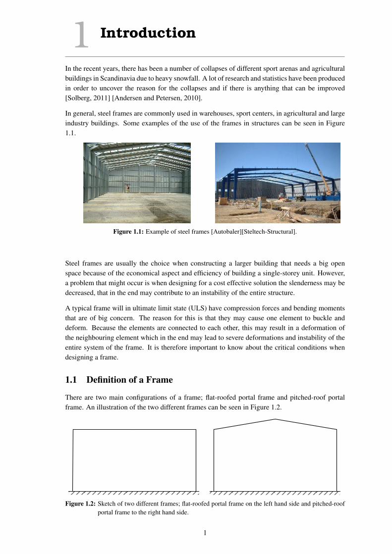
In general, steel frames are commonly used in warehouses, sport centers, in agricultural and largeindustry buildings. Some examples of the use of the frames in structures can be seen in Figure1.1.

Figure 1.1: Example of steel frames [Autobaler][Steltech-Structural].

Steel frames are usually the choice when constructing a larger building that needs a big openspace because of the economical aspect and efficiency of building a single-storey unit. However,a problem that might occur is when designing for a cost effective solution the slenderness may bedecreased, that in the end may contribute to an instability of the entire structure.

A typical frame will in ultimate limit state (ULS) have compression forces and bending momentsthat are of big concern. The reason for this is that they may cause one element to buckle anddeform. Because the elements are connected to each other, this may result in a deformation ofthe neighbouring element which in the end may lead to severe deformations and instability of theentire system of the frame. It is therefore important to know about the critical conditions whendesigning a frame.

1.1 Definition of a Frame

There are two main configurations of a frame; flat-roofed portal frame and pitched-roof portalframe. An illustration of the two different frames can be seen in Figure 1.2.

Figure 1.2: Sketch of two different frames; flat-roofed portal frame on the left hand side and pitched-roofportal frame to the right hand side.

1

1.2 Instability of a Frame

Instability of a frame is of outmost concern. Mainly because instability of frames has lead toseveral collapses of structures, see Figure 1.3

Figure 1.3: Collapse due to lateral torsional buckling [BYG-ERFA].

Instability may occur in members where compression stresses exist, and instability is mostcommon for slender members. The result is buckling of the member and will in the end lead tofailure of the structure. Instability is the result of different buckling modes, and the most commonbuckling modes are:

• Flexural Buckling• Torsional Buckling• Flexural Torsional Buckling• Lateral Torsional Buckling

Flexural Buckling:

According to Eurocode-resources.com, flexural buckling is a phenomena that occurs about theaxis of the highest slenderness ratio and the smallest radius of gyration. It can happen in anymember subjected to compression, which in the end will lead to deflection of the member. Anillustration of the flexural buckling can be seen in Figure 1.4.

2

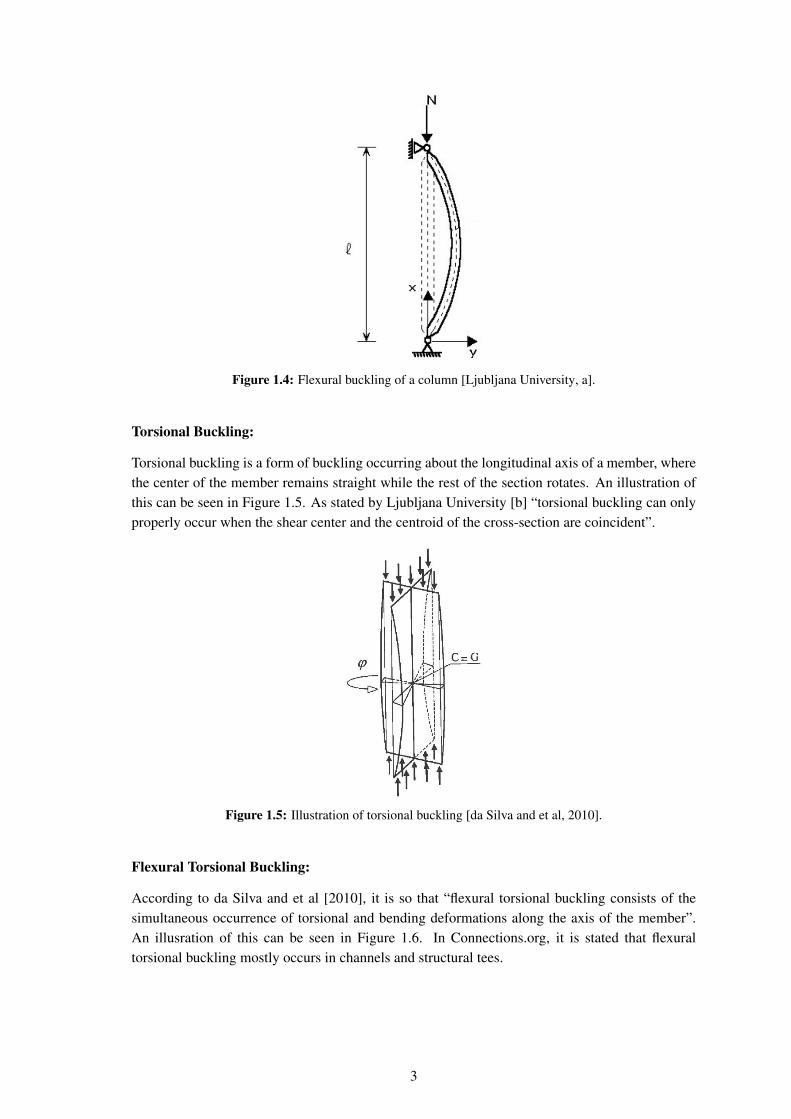
Figure 1.4: Flexural buckling of a column [Ljubljana University, a].

Torsional Buckling:

Torsional buckling is a form of buckling occurring about the longitudinal axis of a member, wherethe center of the member remains straight while the rest of the section rotates. An illustration ofthis can be seen in Figure 1.5. As stated by Ljubljana University [b] “torsional buckling can onlyproperly occur when the shear center and the centroid of the cross-section are coincident”.

Figure 1.5: Illustration of torsional buckling [da Silva and et al, 2010].

Flexural Torsional Buckling:

According to da Silva and et al [2010], it is so that “flexural torsional buckling consists of thesimultaneous occurrence of torsional and bending deformations along the axis of the member”.An illusration of this can be seen in Figure 1.6. In Connections.org, it is stated that flexuraltorsional buckling mostly occurs in channels and structural tees.

3

Figure 1.6: Illustration of flexural torsional buckling [da Silva and et al, 2010].

Lateral Torsional Buckling:

Lateral torsional buckling is as stated in da Silva and et al [2010] “characterized by lateraldeformation of the compressed part of the cross-section”. In an I-section, the compressed partwill be one of the flanges. As a part of the member will behave under compression, it will alsosimultaneously have one continuously restrained by the part of the section in tension. This willresult in a deformation of the cross-section where both lateral and torsion buckling is included.Hence the name lateral torsional buckling [da Silva and et al, 2010].

There is a difference between constrained and unconstrained lateral torsional buckling as theywill behave differently under the buckling process. It is understood that with constrained lateraltorsional buckling means that a point of the member is restrained against deformations across thelength of the member. This means that the axis of rotation is made fixed, which is where themember buckles around, see Figure 1.7 [Bonnerup and et al., 2009].

Flange in

compression

Rotation axis

Bracing

e.g. ceiling

ϕ

F

Figure 1.7: Constrained lateral torsional buckling [Bonnerup and et al., 2009].

4

With unconstrained lateral torsional buckling, the axis of rotation is not given in advance, and it istherefore more complicated to determine the capacity, as it is dependent of the members internalbalance at buckling, see Figure 1.8.

Flange in

compression

Rotation axis

ϕ

F

F

u

Figure 1.8: Unconstrained lateral torsional buckling [Bonnerup and et al., 2009].

The point of application in respect to the load will influence the elastic critical moment of amember. As stated in da Silva and et al [2010] “a gravity load applied below the shear centre C(that coincides with the centroid, in case of doubly symmetric I or H sections) has a stabilizingeffect (Mcr,1 > Mcr), whereas the same load applied above this point has a destabilizing effect(Mcr,2 < Mcr)”. This is illustrated in Figure 1.9.

Figure 1.9: Effect of the point of load’s application [da Silva and et al, 2010].

5

1.2.1 Prevention of Instability

In order to prevent instability and out-of-plane buckling, it is common to use adequate bracings.The bracings must as stated in da Silva and et al [2010] “provide effective restraint to lateraldisplacements of the compressed flange about the minor axis of the cross-section, and shouldprevent the rotation of the cross-section about the longitudinal axis of the member”. There arethree different kinds of bracings that can contribute to prevent the out-of-plane buckling. Theseare:

• Lateral bracings - prevents transverse displacements of the compression flange• Torsional bracings - prevents rotation of a cross-section around its longitudinal axis• Partial bracings - bracing of the tension flange, which however does not fully prevent out-

of-plane buckling, but is equivalent to an elastic support

There are, in addition to bracings, checks that can be done in the Eurocode (EC). The checkswill show whether buckling and lateral torsional effects may be ignored for the member. Thecheck of the buckling effects takes the slenderness of the member into account in addition tothe relationship between the occurring normal force and the critical normal force. In regard oflateral torsional buckling, the slenderness of the member is checked in addition to the relationshipbetween the occurring moment and the critical moment for the section.

1.3 Calculations of a Frame

Nowadays, there are given two different methods by European Standard [2005a] to calculate aframe and to check the frame if it is able to withstand the load applied without any failure. InSection 6.3.3 in European Standard [2005a], Interaction Formulae is introduced. The method isused to see if a member subjected to combined bending and axial compression does not reach autilization over 100%. However, Interaction Formulae can only be applied when the cross-sectionof a member is constant. Today, it is most likely that Interaction Formulae is used even if thecross-section is not constant, as it is easier to use this method and that it is recognized by mostengineers. Eurocode has however come up with another method called the General Method, givenin Section 6.3.4 in European Standard [2005a]. This can be used even if the cross-section of amember is not constant. The general method implies the use of Finite Element Method (FEM) toverify a load amplifier of the design load to reach the characteristic resistance of the most criticalcross-section and the minimum amplifier for the in-plane design loads to reach the elastic criticalresistance. In this way, the method allows for a check to see if the forces and moments acting onthe frame can be resisted by the members of the frame by the use of FEM.

1.4 Aim of the Project

The aim of the project is to examine a frame with respect to instability due to different failuremodes such as flexural buckling and lateral torsional buckling. In order to verify the differentinstabilities of the frame, different methods are used. Two methods from European Standard[2005a] are used where an elastic and plastic analysis is conducted. Then, a third more advancedmethod by the use of FEM is performed. The different methods are then compared to each otherand analysed further to see their limitations and what they take into account. Then, a parameterstudy is conducted to see how different parameters will influence the calculations of the method

6

and the instability of the frame. In the end of the project, a conclusion of the parameter study andthe differences of the two EC methods is given.

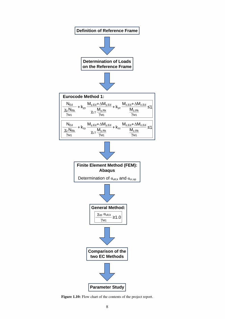
In the beginning of the project, a reference frame of a simple flat-roofed portal frame will beinvestigated. The frame will have profiles given by an assessment of Interaction Formulae in theEC. The loads for the calculation of the structure are based on a real, but simplified, assessmentof loads and load combinations given by the EC. It is also so that EC gives two different ways ofchecking the capacity of a steel frame. These equations will be a part of a further study in orderto investigate how these are used for the capacity of a steel frame. After an investigation of thedifferent methods, a parameter study is done. The parameter study will include the reference framewith unconstrained flanges, with different profiles and with additional fork supports. In addition,the effect of shear wall is also analysed. In the end of the project, comparison and conclusionswill be made in order to understand the different impacts of these parameters. A flow chart of thethe contents of the project can be seen in Figure 1.10.

7

Finite Element Method (FEM):

Abaqus

NEd

χz NRk

γM1

kzy

My,Ed ∆My,Ed

My,RkχLT

≤1++

γM1

kzz

Mz,Ed ∆Mz,Ed

Mz,Rk+

+

γM1

Eurocode Method 1:

General Method:

NEd

χy NRk

γM1

kyy

My,Ed ∆My,Ed

My,RkχLT

≤1++

γM1

kyz

Mz,Ed ∆Mz,Ed

Mz,Rk+

+

γM1

χop

γM1

αult,k≥1.0

Determination of αult,k and αcr,op

Definition of Reference Frame

Determination of Loads

on the Reference Frame

Comparison of the

two EC Methods

Parameter Study

Figure 1.10: Flow chart of the contents of the project report.

8

1.5 Method

In order to achieve the aim of the project and be able to understand the behaviour of a steelframe, a literature study is made to understand the behaviour of a steel frame and the parametersinfluencing this. The focus is on literature explaining the different mechanisms of a frame, butalso on Eurocode 3 part 1-1, where detailed suggestions on how to calculate a steel frame arepresented. In addition, the different Eurocodes containing loads such as imposed load, snow loadand wind load have been simplified but ensured to be a good estimate of the loads in a furtheranalysis of the frame.

In order to make a reasonable comparison between the analytical solution based on the equationsin the EC and the models made in Abaqus/CAE , a further understanding of Abaqus/CAE is alsomade. In this thesis Abaqus/CAE is used to analyse a frame numerically by the Finite ElementMethod (FEM). In addition, a parameter study is also conducted in order to elicit the behaviour ofa steel frame.

1.6 Scope and Limitations

The scope of the project is to look at the two different expressions given by European Standard[2005a] and be able to understand their assumptions and what they take into consideration. FEM isalso used as a part of the General Method in EC and as a more advanced analysis of the frame. It istherefore necessary to be able to understand the basis of FEM and how the software Abaqus/CAEapplies FEM in order to analyse a frame. The scope is also to be able to look at different stabilityproblems and failure modes of a frame, and be able to understand these mechanisms and thesignificant parameters influencing it. In addition, the parameter study is made to get an overviewof the similarities and differences between the two methods from the EC, and to see the correlationthe different parameters have to determine the behaviour of the frame.

There are a number of different parameters which are well suited for an analysis of a frame, butbecause of the extent and complexity of frame, only some parameters has been chosen.

In this project, the basic geometry of the frame will not be changed as some parameters need tobe fixed through out the analysis. In this way, it is possible to see if there are other parametersinfluencing a frame besides the width, depth and height of the structure.

9

2 Reference Frame

The following chapter contains explanations for the choices made before using the two Eurocodemethods to investigate the instability of a frame. In addition, different assumptions andconsiderations about the frame design are given.

2.1 Dimensions

The dimensions of the reference frame constructed in steel can be seen in Figure 2.1. Thedimensions are in accordance to how a steel frame is constructed normally in real life, and thesewill not be varied during this project report.

w = 20 m

d = 6 m

z

x

y

1

2

3 h = 5 m

Figure 2.1: Illustration of the reference frame in a construction.

The circles with a number placed inside in Figure 2.1 and 2.2(

1 , 2 and 3)

are used asreferences for the different elements which in total form the reference frame.

2.2 Statical Model

A reference frame is assumed, and and the statical model of it is shown on Figure 2.2.

11

h = 5 m

w/2 = 10 m

d/2 = 3 m

w = 20 m

d/2 = 3 m

d = 6 m

z

x

yw/2 = 10 m

1

2

3

BAHA HB

VA VB

Figure 2.2: Statical model of the reference frame.

The frame is supported by pinned supports which makes it one time statically indeterminedbecause there is one more reaction, r, than equilibrium equations, e (r = 4, e = 3). Out of theplane, bracings are used to connect the frames which make them pinned supported in that directionas well as seen in Figure 2.2.

The frame is designed as a steel structure where the elements are assumed to have a constantstiffness (E I = constant) depending on in which direction, the investigation is done.

2.3 Profiles

For this project, a HE320A steel profile has been chosen for the reference frame. The real cross-section of a HE320A steel profile is shown on the left hand side in Figure 2.3 while the cross-section assumed in this project report is shown on the right hand side in Figure 2.3. The reasonfor this assumption is that the profile in Abqus/CAE will be according to the profile shown on theright hand side in Figure 2.3. This means that for the analytical assessment, the profile will alsoassumed to have this cross-section.

12

300 mm

310 mm

27 mm

9 mm

15,5 mm

z

z

yy

Real HE320A:

300 mm

310 mm

9 mm

15,5 mm

z

z

yy

Assumed HE320A:

a) b)

Figure 2.3: Steel profile assumption - a) Real HE320A steel profile; b) Assumed HE320A steel profile.

2.4 Material Properties

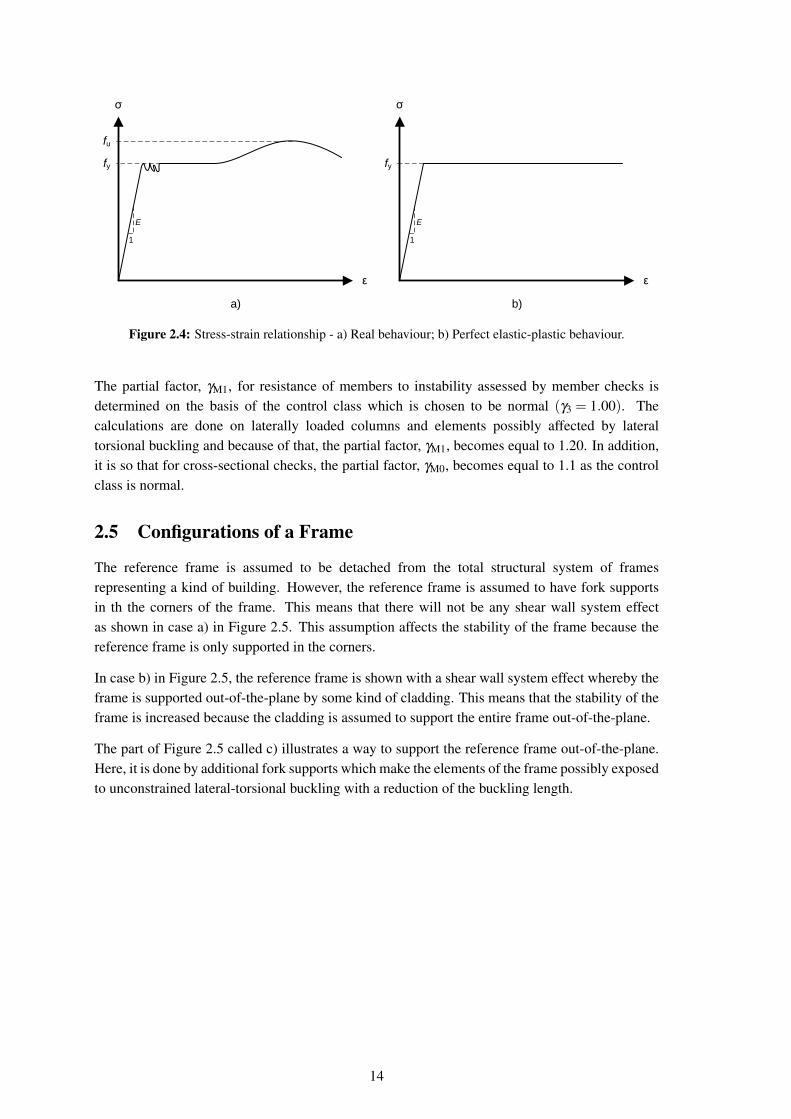
It has been chosen to work with a frame consisting of steel S235. The general material propertiesfor construction steel S235 are given in Table 2.1. The behaviour of the steel is considered perfectelastic-plastic, and the stress-strain relationship is shown in Figure 2.4. It is the Von Mises platicitywhich is used. The diagram shown on the left hand side is the real behaviour of steel while thediagram shown on the right hand side is the assumed behaviour used in this project report.

Description Symbol Value Unit

Yield Strength of Construction Steel S235 fy 235 [MPa]

Modulus of Elasticity E 210000 [MPa]

Shear Modulus G 81000 [MPa]

Density ρ 7850 [kg/m3]

Poisson’s Ratio ν 0.3 [-]

Table 2.1: Material properties for construction steel S235.

13

ε

σσ

ε

fy

fu

fy

E

1

E

1

a) b)

Figure 2.4: Stress-strain relationship - a) Real behaviour; b) Perfect elastic-plastic behaviour.

The partial factor, γM1, for resistance of members to instability assessed by member checks isdetermined on the basis of the control class which is chosen to be normal (γ3 = 1.00). Thecalculations are done on laterally loaded columns and elements possibly affected by lateraltorsional buckling and because of that, the partial factor, γM1, becomes equal to 1.20. In addition,it is so that for cross-sectional checks, the partial factor, γM0, becomes equal to 1.1 as the controlclass is normal.

2.5 Configurations of a Frame

The reference frame is assumed to be detached from the total structural system of framesrepresenting a kind of building. However, the reference frame is assumed to have fork supportsin th the corners of the frame. This means that there will not be any shear wall system effectas shown in case a) in Figure 2.5. This assumption affects the stability of the frame because thereference frame is only supported in the corners.

In case b) in Figure 2.5, the reference frame is shown with a shear wall system effect whereby theframe is supported out-of-the-plane by some kind of cladding. This means that the stability of theframe is increased because the cladding is assumed to support the entire frame out-of-the-plane.

The part of Figure 2.5 called c) illustrates a way to support the reference frame out-of-the-plane.Here, it is done by additional fork supports which make the elements of the frame possibly exposedto unconstrained lateral-torsional buckling with a reduction of the buckling length.

14

a) no effect of shear wall system b) effect of shear wall system

c) additional fork supports

z

x

y

Figure 2.5: Effect of Shear Wall System - a) No effect of shear wall system; b) Effect of shear wall system;c) Additional fork supports.

If the reference frame is modelled as in case b) or c), the situation regarding the lateral torsionalbuckling changes because the supporting conditions of the elements forming the referenceframe change. Thereby, the elements switch from being possibly exposed to unconstrained toconstrained lateral torsional buckling.

15

3 Loads

Normally, a frame is exposed to the following four kinds of load types:

• Permanent Loads• Snow Load• Wind Loads• Imposed Load

In this chapter, a quick assessment and explanation of the determined loads will be done. Inaddition, the load combinations will be stated so that in the end, the final load scenario of theframe is found.

3.1 Permanent Loads

The permanent load of the considered frame is its self-weight. The self-weight of the frame iscalculated for the different profiles used in the analysis. The permanent load of the frame is givenin Table 3.1. It is chosen to have a HE320A profile on the frame, where in Appendix B, an exampleof how the right profile is found can be seen. HE320A is a profile that satisfies the equations ofmethod 1 in the Eurocode (see eq. 4.1 and 4.2 in section 4.1).

Profile Weight Permanent load

HE320A 97.6 kg/m 0.957 kN/m

Table 3.1: Self-weight of HE320A steel profile.

In addition, the load on the roof of the structure is taken as a light weight roof of 0.50 kN/m2

[Lett-Tak Systemer AS]. Also, the cladding of the structure needs to be taken into consideration.It is therefore chosen that the load of the cladding will be the same as for the roof (0.50 kN/m2).

3.2 Snow Load

The snow load is a variable load as the loading is not constant during the year. The snow load willin general vary depending on the location of the structure, the slope angle of the roof, contributionand interference of other roofs and contribution and drifting at projections and obstructions.

In this project, the characteristic snow load is calculated to be 0.72 kN/m2. The calculations aredone by following European Standard [2007a]. The calculations are based on a frame with a slopeangle of 0◦, as this is the most critical case. In addition, the frame is assumed to have a location ofnormal topography. Most commonly, sports arenas, industry and agricultural buildings are placedin more remote/outlying locations, which means that the topography will be windswept. However,this will result in a lower snow load, and it will therefore not be applicable in this case.

3.3 Wind Loads

The wind load is calculated based on European Standard [2007b]. The wind has been calculatedfrom the west direction as the highest wind load will occur in this direction. Also, the frame is

17

subjected to wind during the whole year, giving it the most critical seasonal factor. The terraincategory is chosen to be of category II, corresponding to a location at the countryside, meaningthat the frame may have a few obstacles like trees and buildings around. This corresponds to thesame topography as used in the snow load calculation.

A simplification of the wind load has been made in regards of the wind pressure on the roof andthe internal pressure. The calculations show both a suction on some parts of the roof and pressureon other parts. The different parts are depended on the width of the structure. A simplification istherefore made to ignore wind loads on the roof and the internal pressure.

The calculations of characteristic wind load shows a windward pressure of 0.49 kN/m2 and anegative leeward pressure of -0.21 kN/m2. This is also illustrated in Figure 3.1.

3.4 Imposed Load

The imposed load is taken from section 6.3.4 in European Standard [2002] where category H isclassified as “roofs not accessible except for normal maintenance and repair” [European Standard,2002], which will be the case for the frame. In the national annex, a value of 0 kN/m2 is given tothis category, meaning that the frame will not have any imposed load.

3.5 Summary of Loads

Self-weight Roof Cladding

0.957 kN/m 0.5 kN/m2 0.5 kN/m2

Table 3.2: Permanent loads.

Snow load Wind load, windward Wind load, leeward Imposed load

0.72 kN/m2 0.49 kN/m2 -0.21 kN/m2 0 kN/m2

Table 3.3: Summary of the variable loads.

The load situation on the frame is illustrated in Figure 3.1.

Load

leeward

Load roof

Load

windward

z

x

y

Figure 3.1: Principle sketch of loads on a frame.

18

3.6 Load Combinations and Loads on the Reference Frame

The following equation is used for calculating the load combination:

Permanent actions Leading variable Accompanying variable

ξ KFI γGj,sup Gkj,sup KFI γQ,1 Qk,1 KFI γQ,i ψ0,i Qk,i

Table 3.4: Design values of actions (STR/GEO) [European Standard, 2005b].

Gkj,sup Upper/lower characteristic value of permanent action j [kN/m]Qk,1 Characteristic value of the leading variable action 1 [kN/m2]Qk,i Characteristic value of the accompanying variable action i [kN/m2]ξ Reduction factor, given in Table 3.5 [-]

KFI Consequence class factor, given in Table 3.5 [-]γGj,sup , γQ,i Partial factors, given in Table 3.5 [-]

ψ0,i Factor for combination value of a variable action i, given in Table 3.5 [-]

Description Symbol Value

Reduction factor ξ 1.0

Consequence class factor for CC2 KFI 1.0

Partial factor for permanent action jγGj,sup 1.0

in calculating upper/lower design values

Partial factor for variable action i γQ,i 1.5

Factor for combination valueψ0,i 0.3

of a variable action i

Table 3.5: Different safety factors given in European Standard [2005b].

From this, the following load combination factors can be calculated.

Permanent load Leading variable Accompanying variable

1.0 ·1.0 ·1.0 ·Gkj,sup 1.0 ·1.5 ·Qk,1 1.0 ·1.5 ·0.3 ·Qk,i

Table 3.6: Load combination factors.

When the load combination factors are used, the value of the loads can be calculated. The differentload combinations that can be used is when snow is dominant and when wind is dominant. Whenthe wind is dominant, no snow load is applied. The loads are calculated for a span of 6 m (seechapter 2).

Dominant load Permanent load Leading variable

Snow 1.0 · (0.957 kN/m+(0.5 kN/m2 ·6 m)) 1.5 · (0.72 kN/m2 ·6 m)

Wind 1.0 · (0.957 kN/m+(0.5 kN/m2 ·6 m)) 1.5 · (0.49 kN/m2 ·6 m )

19

Dominant load Accompanying variable Accompanying variable 2

Snow 0.45 · (0.49 kN/m2 ·6 m) 0.45 · (−0.21 kN/m2 ·6 m)

Wind 0.45 · (−0.21 kN/m2 ·6 m) -

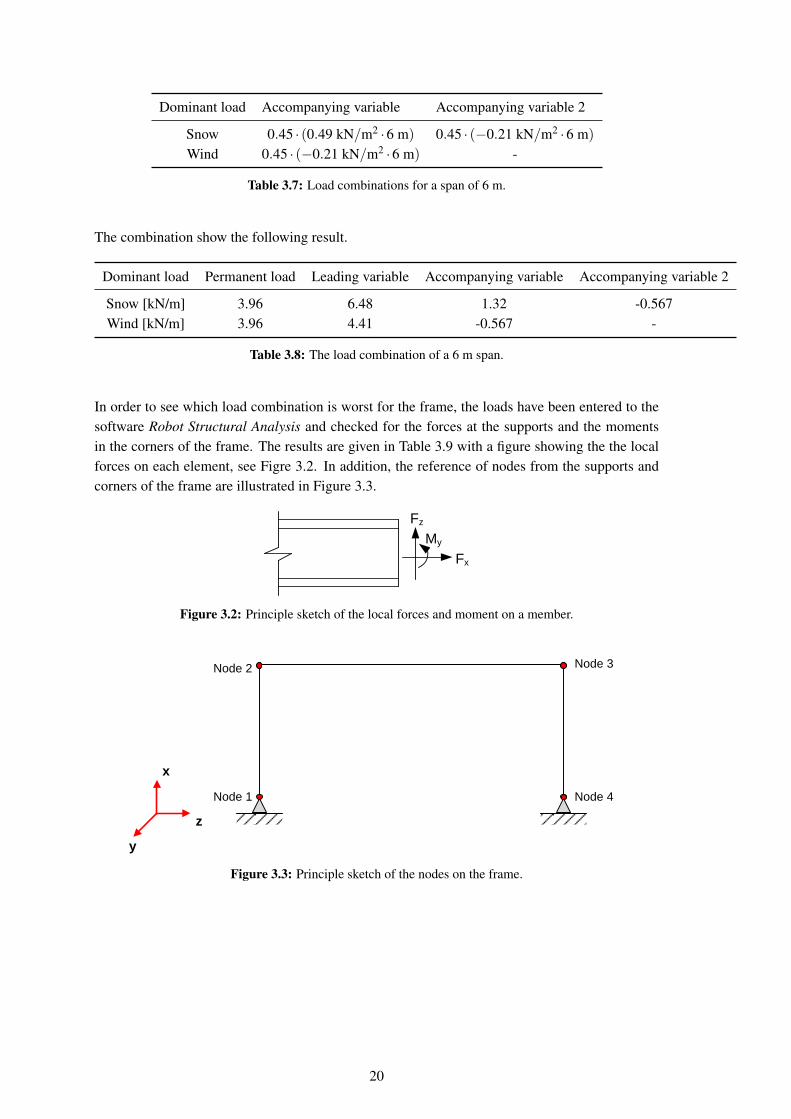
Table 3.7: Load combinations for a span of 6 m.

The combination show the following result.

Dominant load Permanent load Leading variable Accompanying variable Accompanying variable 2

Snow [kN/m] 3.96 6.48 1.32 -0.567Wind [kN/m] 3.96 4.41 -0.567 -

Table 3.8: The load combination of a 6 m span.

In order to see which load combination is worst for the frame, the loads have been entered to thesoftware Robot Structural Analysis and checked for the forces at the supports and the momentsin the corners of the frame. The results are given in Table 3.9 with a figure showing the the localforces on each element, see Figre 3.2. In addition, the reference of nodes from the supports andcorners of the frame are illustrated in Figure 3.3.

My

Fx

Fz

Figure 3.2: Principle sketch of the local forces and moment on a member.

Node 4Node 1

Node 3Node 2

z

x

y

Figure 3.3: Principle sketch of the nodes on the frame.

20

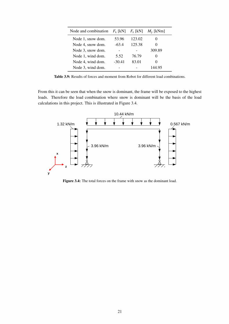
Node and combination Fx [kN] Fz [kN] My [kNm]

Node 1, snow dom. 53.96 123.02 0Node 4, snow dom. -63.4 125.38 0Node 3, snow dom. - - 309.89Node 1, wind dom. 5.52 76.79 0Node 4, wind dom. -30.41 83.01 0Node 3, wind dom. - - 144.95

Table 3.9: Results of forces and moment from Robot for different load combinations.

From this it can be seen that when the snow is dominant, the frame will be exposed to the highestloads. Therefore the load combination where snow is dominant will be the basis of the loadcalculations in this project. This is illustrated in Figure 3.4.

0.567 kN/m

10.44 kN/m

1.32 kN/m

3.96 kN/m 3.96 kN/m

z

x

y

Figure 3.4: The total forces on the frame with snow as the dominant load.

21

4 Analytical Analysis

The following chapter of the project contains the analytical analysis of the reference framepresented in Chapter 2. The analytical analysis conducted is by the Interaction Formulae foundin Eurocode 3 [European Standard, 2005a] where the method takes uniform members in bendingand axial compression into account. The method is used to see if a member can resist the bendingand axial compression it is subjected to. In this chapter, a description of important parameters andassumptions are stated, in addition to the limitations of Method 1. In the end, the results for theInteraction Formulae for the reference frame is given.

4.1 Eurocode - Method 1

In European Standard [2005a], the following expressions must be satisfied for a member which issubjected to combined bending and axial compression, see Eq.4.1 and 4.2.

NEdχy NRk

γM1

+ kyyMy,Ed +∆My,Ed

χLTMy,RkγM1

+ kyzMz,Ed +∆Mz,Ed

Mz,RkγM1

≤ 1 (4.1)

NEdχz NRk

γM1

+ kzyMy,Ed +∆My,Ed

χLTMy,RkγM1

+ kzzMz,Ed +∆Mz,Ed

Mz,RkγM1

≤ 1 (4.2)

NEd , My,Ed , Mz,EdDesign values of the compression force and the maximum moments

[-]about the y-y and z-z axis along the member, respectively

∆My,Ed , ∆Mz,Ed Moments due to the shift of the centroidal axis for class 4 sections [-]

χy , χz Reduction factors due to flexural buckling [-]

χLT Reduction factor due to lateral torsional buckling [-]

kyy , kyz , kzy , kzz Interaction factors [-]

In addition, Table 6.7 in Eurocode 3 part 1-1 explains the following values as seen i Eq. (4.3) and(4.3).

NRk = fy Ai (4.3)

Mi,Rk = fy Wi (4.4)

fy Yield strength[N/mm2]

Ai Area[mm2

]Wi Section modulus

[mm3

]This means that the following equations can be written, see Eq. (4.5) and (4.6).

NEdχy fyAi

γM1

+ kyyMy,Ed +∆My,Ed

χLTfyWiγM1

+ kyzMz,Ed +∆Mz,Ed

fyWiγM1

≤ 1 (4.5)

NEdχz fyAi

γM1

+ kzyMy,Ed +∆My,Ed

χLTfyWiγM1

+ kzzMz,Ed +∆Mz,Ed

fyWiγM1

≤ 1 (4.6)

23

4.1.1 Important Parameters and Assumptions

In this section, a short introduction to the major parameters of Eq. (4.5) and (4.6) are presented.There are also examples given on how different parameters change due to different assumptions,showing how Eq. (4.5) and (4.6) may be influenced due to different assumptions.

The references made to this section are from Eurocode 3 European Standard [2005a].

Reduction Factor for Relevant Buckling Mode, χ:

The reduction factor for the relevant buckling curve, χ , is calculated for both y- and z-axis by theequation seen in Eq. (4.7).

χ =1

Φ+

√Φ2−λ

2, χ ≤ 1 (4.7)

Φ is used to determine the reduction factor. It is calculated as seen in Eq. (4.8).

Φ = 0.5(

1+α

(λ −0.2

)+λ

2)

(4.8)

The non-dimensional slenderness, λ is calculated as follows the following equation, see (4.9).

λ =

√A fy

Ncr(4.9)

Ncr Elastic critical force [N]

The critical parameter when determining either χy or χz is Ncr. Ncr is calculated as seen in Eq.(4.10).

Ncr =π2 E I

l2s

(4.10)

E Young’s Modulus[N/mm2]

I Moment of Inertia[mm4

]ls Effective length [mm]

In Eq. (4.10), ls is the effective length of the buckling length of a member. The effective lengthis calculated from the original length of the member multiplied by an effective length factor, K.The factors are depending on the different support conditions. An illustration of this can be seenin Figure 4.1.

24

Figure 4.1: Effective length factors [Wikipedia].

In order to see how χ will change by using a different effective length factor, an example has beenmade where χy and χz is calculated for the reference frame for both element 2 and 3 . Theresults can be seen in Table 4.1.

Effective Element 2 Element 3length, ls χy [-] χz [-] χy [-] χz [-]

2.0 ·L 0.0918 0.030 0.735 0.356

1.0 ·L 0.320 0.110 0.930 0.730

0.5 ·L 0.735 0.356 1.0 0.926

Table 4.1: Different χ depending on the effective length of the members of the reference frame.

As it can be seen in Table 4.1, χ is depending on the effective length, ls. Therefore, it is importantwhen designing for a frame, that the assumptions of the effective length are as close to the realityas possible. If not, then as seen in Table 4.1, the reduction factor, χ , may have great impact whenEq. (4.5) and (4.6) is calculated i the end.

The imperfection factor α is also used to determine χ , where α depends on the relationship ofh/b and if the section is welded or rolled. However, for the calculation of χ for the referenceframe, there is no difference between α as long as the thickness of the flange, tf, is below 40 mm(tf ≥ 40 mm). This means that for this project the α factor is constant.

Reduction Factor for Lateral Torsional Buckling Curves, χLT:

There are two different ways of determining χLT. There is a general method and a second methodthat is applicable for rolled or equivalent welded sections. From European Standard [2005a], it canbe seen from the equations used to calculate χLT, that choosing the first general method will givea lower value than the second method of rolled or equivalent sections. However, as the referenceframe consists of a rolled or equivalent section, the second method is used for the calculation.

When choosing the second method, European Standard [2005a] states that χLT may be modified.The modification value, f, can be found in the Danish National Annex where it is stated that f = 1as the moment distribution is included in the determination of Mcr. This means that in this case,χLT is not modified.

25

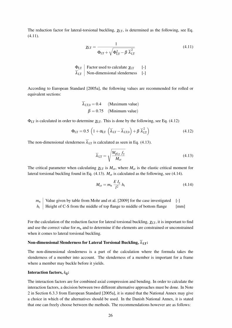
The reduction factor for lateral-torsional buckling, χLT, is determined as the following, see Eq.(4.11).

χLT =1

ΦLT +

√Φ2

LT−β λ2LT

(4.11)

ΦLT Factor used to calculate χLT [-]λ LT Non-dimensional slenderness [-]

According to European Standard [2005a], the following values are recommended for rolled orequivalent sections:

λ LT,0 = 0.4 (Maximum value)

β = 0.75 (Minimum value)

ΦLT is calculated in order to determine χLT. This is done by the following, see Eq. (4.12)

ΦLT = 0.5(

1+αLT

(λ LT−λ LT,0

)+β λ

2LT

)(4.12)

The non-dimensional slenderness λ LT is calculated as seen in Eq. (4.13).

λ LT =

√Wpl,y fy

Mcr(4.13)

The critical parameter when calculating χLT is Mcr, where Mcr is the elastic critical moment forlateral torsional buckling found in Eq. (4.13). Mcr is calculated as the following, see (4.14).

Mcr = mnE Iz

l2 ht (4.14)

mn Value given by table from Mohr and et al. [2009] for the case investigated [-]ht Height of C-S from the middle of top flange to middle of bottom flange [mm]

For the calculation of the reduction factor for lateral torsional buckling, χLT, it is important to findand use the correct value for mn and to determine if the elements are constrained or unconstrainedwhen it comes to lateral torsional buckling.

Non-dimensional Slenderness for Lateral Torsional Buckling, λ LT:

The non-dimensional slenderness is a part of the calculation where the formula takes theslenderness of a member into account. The slenderness of a member is important for a framewhere a member may buckle before it yields.

Interaction factors, kij:

The interaction factors are for combined axial compression and bending. In order to calculate theinteraction factors, a decision between two different alternative approaches must be done. In Note2 in Section 6.3.3 from European Standard [2005a], it is stated that the National Annex may givea choice in which of the alternatives should be used. In the Danish National Annex, it is statedthat one can freely choose between the methods. The recommendations however are as follows:

26

“Method 1 is recommended for significant structures, when economy is crucial and by preparationof a calculation software” [European Standard, 2005a].

“Method 2 is recommended as a more simplifying method at less significant structures”[EuropeanStandard, 2005a].

Even though economy plays an important role when constructing a frame, this project does notprepare for a calculation program. In addition, the frame is not a significant structure. This meansthat for this project, the second more simplifying method is chosen for the calculation of theinteraction factors.

An important decision to make when determining the interaction factors is choosing the rightmoment distribution diagram to follow. The European Standard [2005a] gives a standard momentdistribution diagram for method 2 that can be seen in Figure 4.2.

Figure 4.2: Equivalent uniform moment factors Cm [European Standard, 2005a].

The factor Cmy is included in the calculation of the interaction factor kij. In order to illustrate howit is possible to determine different moment diagrams for the same element, an example is givenof element 3 . Element 3 has originally a moment diagram distribution of a triangle, whereat the bottom of the support, the moment equals zero, see Figure 4.3. However, if the effectivelength used to determine χ is taken into account, the moment distribution changes. This meansthat if an effective length of two times the original length is used, Cmy and in the end kyy and kzy

will change. This is illustrated in Figure 4.3.

27

309.89 kNm309.89 kNmLeff

L

Figure 4.3: Different moment distributions according to original length and effective length of element 3.

The different Cmy, kyy and kzy based on the different moment distributions are compared to eachother in Table 4.2.

Moment distribution from Cmy [-] kyy [-] kzy [-]

Original length 0.6 0.984 0.590

Effective length 0.95 0.623 0.373

Table 4.2: kyy and kzy calculated for different moment distributions on element 3 .

From Table 4.2, it can be seen that there is a significant difference in the kyy and kzy factorsdepending on the moment distribution chosen. The question then becomes if the momentdistribution should be according to the effective length of the member or to the original lengthof the member.

It should also be stated that kzz and kyz equals zero as there is no moment about the z-axis.

4.2 Limitations of Interaction Formulae

In order to use the equations given for the Interaction Formula, which takes uniform members inbending and axial compression into account, it is required, according to Eurocode 3 [EuropeanStandard, 2005a], that the member consists of a profile with constant cross-section. If a membervaries in the cross-section, the General Method, should be used. How the General Method isapplied can be seen in Chapter 5.

28

4.3 Calculation of a Frame Profile

All of the calculations of the frame has been calculated in MATLAB-codes. The codes can beseen in the Digital Appendix, see A.11 and A.12.

Interaction Formulae is used to calculate a profile that is suited for the reference frame. In order tofind a suited profile, a MATLAB code has been made. The program is calculating the utilizationratio for the Interaction Formulae by using Equation (4.1) and (4.2). The input parameters of theprogram are the section properties, the compression force and moment, and different assumptionssuch as the effective length of buckling and of lateral torsional buckling and Cmy. Different profileshave been investigated to find a profile with the utilization ratio closes to 1.0 (100%). In AppendixB, a worked example of a HE320A profile has been done. The calculation is an elaboration onhow method 1 is implemented.

The MATLAB code has been used for the investigation of HE320A. The profile will be usedfor the reference frame so that the utilization ratio for Method 1 and the General Method can becompared.

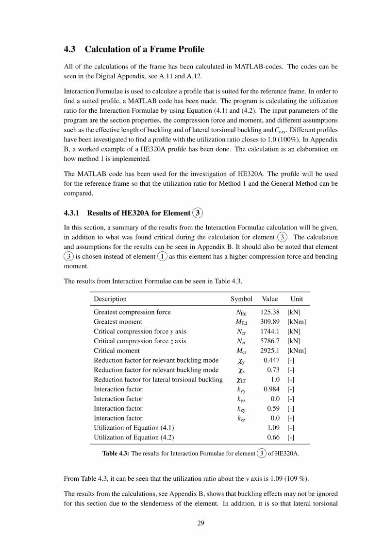
4.3.1 Results of HE320A for Element 3

In this section, a summary of the results from the Interaction Formulae calculation will be given,in addition to what was found critical during the calculation for element 3 . The calculationand assumptions for the results can be seen in Appendix B. It should also be noted that element3 is chosen instead of element 1 as this element has a higher compression force and bending

moment.

The results from Interaction Formulae can be seen in Table 4.3.

Description Symbol Value Unit

Greatest compression force NEd 125.38 [kN]Greatest moment MEd 309.89 [kNm]Critical compression force y axis Ncr 1744.1 [kN]Critical compression force z axis Ncr 5786.7 [kN]Critical moment Mcr 2925.1 [kNm]Reduction factor for relevant buckling mode χy 0.447 [-]Reduction factor for relevant buckling mode χz 0.73 [-]Reduction factor for lateral torsional buckling χLT 1.0 [-]Interaction factor kyy 0.984 [-]Interaction factor kyz 0.0 [-]Interaction factor kzy 0.59 [-]Interaction factor kzz 0.0 [-]Utilization of Equation (4.1) 1.09 [-]Utilization of Equation (4.2) 0.66 [-]

Table 4.3: The results for Interaction Formulae for element 3 of HE320A.

From Table 4.3, it can be seen that the utilization ratio about the y axis is 1.09 (109 %).

The results from the calculations, see Appendix B, shows that buckling effects may not be ignoredfor this section due to the slenderness of the element. In addition, it is so that lateral torsional

29

buckling effects may be ignored and only cross-sectional checks will apply.

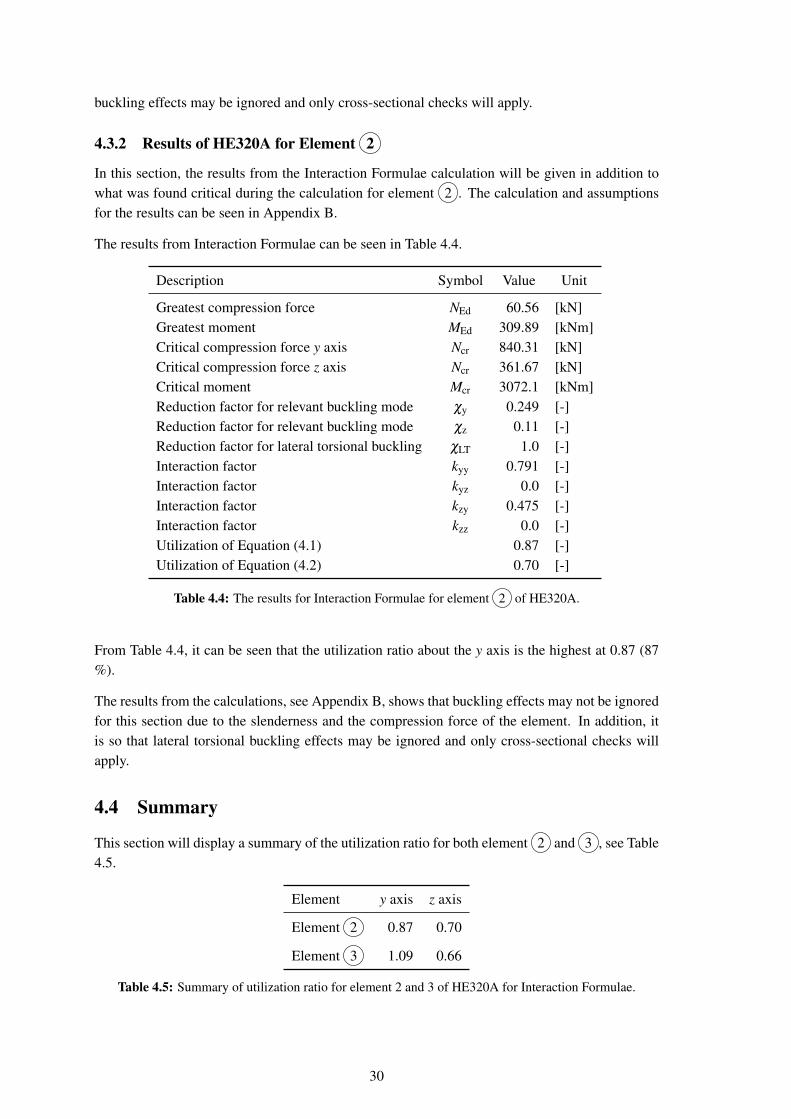
4.3.2 Results of HE320A for Element 2

In this section, the results from the Interaction Formulae calculation will be given in addition towhat was found critical during the calculation for element 2 . The calculation and assumptionsfor the results can be seen in Appendix B.

The results from Interaction Formulae can be seen in Table 4.4.

Description Symbol Value Unit

Greatest compression force NEd 60.56 [kN]Greatest moment MEd 309.89 [kNm]Critical compression force y axis Ncr 840.31 [kN]Critical compression force z axis Ncr 361.67 [kN]Critical moment Mcr 3072.1 [kNm]Reduction factor for relevant buckling mode χy 0.249 [-]Reduction factor for relevant buckling mode χz 0.11 [-]Reduction factor for lateral torsional buckling χLT 1.0 [-]Interaction factor kyy 0.791 [-]Interaction factor kyz 0.0 [-]Interaction factor kzy 0.475 [-]Interaction factor kzz 0.0 [-]Utilization of Equation (4.1) 0.87 [-]Utilization of Equation (4.2) 0.70 [-]

Table 4.4: The results for Interaction Formulae for element 2 of HE320A.

From Table 4.4, it can be seen that the utilization ratio about the y axis is the highest at 0.87 (87%).

The results from the calculations, see Appendix B, shows that buckling effects may not be ignoredfor this section due to the slenderness and the compression force of the element. In addition, itis so that lateral torsional buckling effects may be ignored and only cross-sectional checks willapply.

4.4 Summary

This section will display a summary of the utilization ratio for both element 2 and 3 , see Table4.5.

Element y axis z axis

Element 2 0.87 0.70

Element 3 1.09 0.66

Table 4.5: Summary of utilization ratio for element 2 and 3 of HE320A for Interaction Formulae.

30

From 4.5, it can be seen that the worst element of the frame is element 3 as this element has autilization ratio above 100%. The utilization ratio about the z axis is also higher for element 3than element 2 .

31

5 General Method

The following chapter contains an investigation of the reference frame presented in Chapter 2by the General Method [European Standard, 2005a]. The General Method allows to make useof a Finite Element Analysis (FEA) to determine the two load amplifiers, αult,k and αcr,op, cf.Section 5.1. Therefore, the engineering simulation program Abaqus/CAE is used to perform theanalysis because it makes use of the Finite Element Method (FEM). Brief descriptions of thebackground for the Finite Element Method (FEM) and Abaqus/CAE are given in Appendix C andD, respectively.

5.1 General Method

The General Method is a method described in Section 6.3.4 in European Standard [2005a] toinvestigate if lateral and lateral torsional buckling of structural components occur, and it takes intoaccount the out-of-plane stability of a frame by a global reduction factor, χop. The method canbe used where the method explained in Chapter 4 does not apply e.g. when the C-S of the steelprofile used is varying in dimensions. Eq. (5.1) shows the condition which has to be fulfilled forthe frame to resist out-of-plane buckling for any of the structural components.

χop αult,k

γM1≥ 1.0 (5.1)

αult,k

Minimum load amplifier of the design loads to reach the charac-

[-]

teristic resistance of the most critical cross-section of the structu-ral component considering its in-plane behaviour without takinglateral or lateral torsional buckling into account however account-ing for all effects due to in-plane geometrical deformation and im-perfections, global and local, where relevant

χop Global reduction factor for the non-dimensional slenderness λ op [-]

γM1Partial factor for resistance of members to instability assessed by

[-]member checks, γM1 = 1.20

One of the difficult parameters to determine by a hand calculation is the mininum load amplifier,αult,k. This minimum load amplifier can be determined by a non-linear analysis of a framemodelled by two-dimensional beam elements on which the loads are increasing incrementally.Even though the model is two-dimensional, the analysis remains geometrically and materiallynon-linear, and in-plane bow and sway imperfections are taken into account by the analysis whererelevant, but out-of-plane sway imperfections are not included. Appendix E describes how to takethese imperfections into account.

The global reduction factor for out-of-plane buckling, χop, is determined by another parameterwhich is also difficult to determine by a hand calculation. That parameter is the minimum loadamplifier, αcr,op, for the in-plane design loads to reach the elastic critical resistance of the structuralcomponent with regards to lateral or lateral torsional buckling without accounting for in-planeflexural buckling, which can be evaluated by modelling the frame with three-dimensional shellelements.

The General Method is advantageous compared to the method used in Chapter 4 since it is ableto take into account e.g. varying C-S of the members of the frame. It is a numerical method and

33

Finite Element (FE) software may be used to determine the two load amplifiers contained in Eq.(5.1).

As described in Appendix C, the Finite Element Method (FEM) contains three steps - aPreprocessing, Simulation and Postprocessing step. These steps and the contents of themaccording to the numerical analysis performed on the reference frame are described in thefollowing sections. The results of the analysis and the determination of the two load amplifiers areshown in the Postprocessing step in Section 5.4.

5.2 Preprocessing

In the Preprocessing step, the reference frame is modelled in Abaqus/CAE as described in Chapter2 where the statical model and thereby also the boundary conditions of the frame are set up. Thegeometry of the frame is shown in Figure 2.2, and the material properties are given in Table 2.1.The most critical load scenario for the frame is found in Chapter 3.

5.2.1 Finite Element Types

It is of great importance when analysing a finite element model to apply the appropriate type ofelement to the model being analysed. Abaqus/CAE has access to a database containing a largenumber of different element types categorized based on family, degrees of freedom, number ofnodes, order of interpolation, formulation and integration.

The given reference frame is modelled by two different types of finite elements - beam elementsand shell elements shown to the left and to the right in Figure 5.1, respectively. The differencebetween beam and shell elements is that the beam elements are one-dimensional and are used formodelling structures in which one dimension (the length) is significantly greater than the other twodimensions and in which the longitudinal stress is most important. In contrast to beam elements,shell elements are two-dimensional and are used for modelling structures in which one dimension(the thickness) is significantly smaller than the other two dimensions and in which the stresses inthe thickness direction are negligible.

Figure 5.1: Beam elements and shell elements [SIMULIA, 2012].

The choice of finite element type and the number of finite elements influence the level of detail ofthe model. The level of detail of the model increases by using shell elements compared to beamelements because the number of finite elements increases. However, the computation time is alsoincreasing when using shell elements instead of beam elements.

5.2.2 Modelling by Beam Elements

Firstly, the reference frame is modelled by the simpler beam elements to give a preliminaryestimate of the behaviour of the frame due to instability and to determine the minimum load

34

amplifier, αult,k, cf. Section 5.1. The C-S of the applied steel profile has to be defined when usingbeam elements to model the frame. This is done by defining a generalised beam profile using C-Sengineering properties - in this case of an I-beam. The C-S properties of a HE320A profile, whichis the beam profile used, are shown in Table B.2. In Abaqus/CAE, beam elements are modelledas lines. Therefore, the figures in the following sections are illustrated with a graphical optionswitch on to show the C-S of the steel profile used to model the reference frame. The units used inAbaqus/CAE for the beam element model are millimetres [mm] for the dimensions, megapascals[MPa] for the modulus of elasticity, E, and thus newtons per millimetre [N/mm] for the loads.This can be seen in Figure 5.2. The beam element model made in Abaqus/CAE can be found inDigital Appendix A.1.

x

z

y

0.567 N/mm

10.44 N/mm

1.32 N/mm 3.96 N/mm 3.96 N/mm

20000 mm

5000 mm

Figure 5.2: Units used in the beam element model in Abaqus/CAE.

Mesh

The beam element model is constructed of 2-noded linear beam elements in space. The meshedbeam element model is shown in Figure 5.3.

Figure 5.3: Mesh of the beam element model shown in 2D.

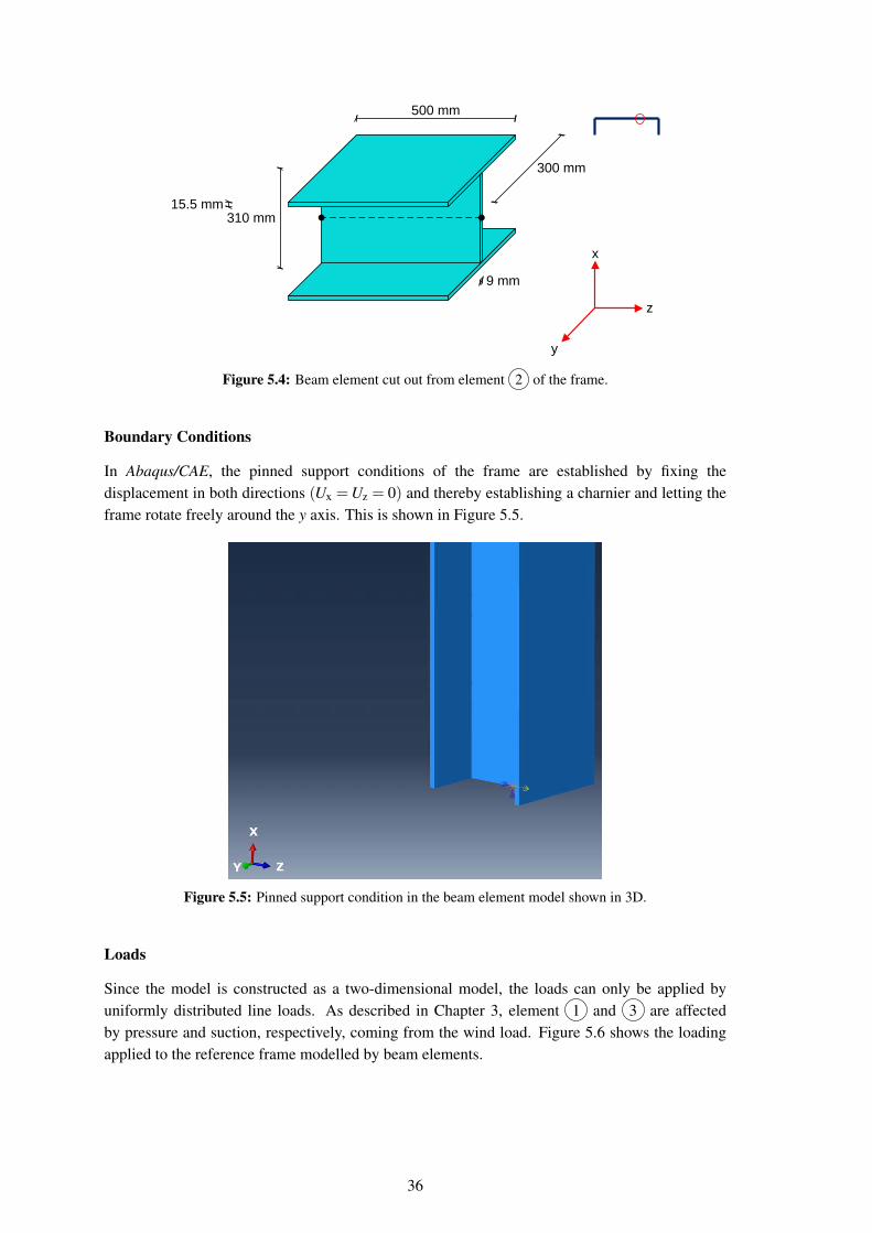
The discretization of the beam element model is set to 500, and this results in an element size inthe length scale of 500 mm. A beam element cut out from element 2 of the frame is shown inFigure 5.4. The black dots in the figure are the two nodes representing the beam element.

35

500 mm

300 mm

310 mm

x

z

y

15.5 mm

9 mm

Figure 5.4: Beam element cut out from element 2 of the frame.

Boundary Conditions

In Abaqus/CAE, the pinned support conditions of the frame are established by fixing thedisplacement in both directions (Ux =Uz = 0) and thereby establishing a charnier and letting theframe rotate freely around the y axis. This is shown in Figure 5.5.

Figure 5.5: Pinned support condition in the beam element model shown in 3D.

Loads

Since the model is constructed as a two-dimensional model, the loads can only be applied byuniformly distributed line loads. As described in Chapter 3, element 1 and 3 are affectedby pressure and suction, respectively, coming from the wind load. Figure 5.6 shows the loadingapplied to the reference frame modelled by beam elements.

36

Figure 5.6: Uniformly distributed line load applied to the reference frame modelled by beam elementsshown in 2D.

5.2.3 Modelling by Shell Elements

To do a more detailed analysis of the behaviour of the reference frame due to instability and todetermine the other minimum load amplifier, αcr,op, the frame is modelled by the more advancedshell elements. The modelling of the frame by shell elements is done separately meaning that thetwo flanges and the web are modelled individually by parts and afterwards merged together. Theunits used in Abaqus/CAE for the shell element model are millimetres [mm] for the dimensions,megapascals [MPa] for the modulus of elasticity, E, and thus newton per square millimetres[N/mm2] for the pressures applied as the loads. This can be seen in Figure 5.7. The self-weightof the reference frame is inflicted by specifying the density of steel, ρ , and applying gravity(g = 9.81 N/kg) to it as well. The shell element model made in Abaqus/CAE can be found inDigital Appendix A.3.

x

z

y 20000 mm

5000 mm

0.0216 N/mm2

0.0044 N/mm2

0.00189 N/mm2

Figure 5.7: Units used in the shell element model in Abaqus/CAE.

Mesh

The shell element model is constructed of 4-noded doubly curved shell elements. The meshedshell element model is shown in Figure 5.8.

37

Figure 5.8: Mesh of the shell element model shown in 3D.

The discretization of the shell element model is chosen to be 80 which results in an element lengthof 80 mm as shown in Figure 5.9. Figure 5.9 also shows the dimensions of the shell elementsrepresenting the flanges and the web, respectively, of a cut out of element 2 . The black dots onthe elements are the four nodes representing the shell element.

x

z

y

80 mm

80 mm

69.75 mm

15.5 mm75 mm

9 mm

WEBFLANGES

80 mm80 mm

69.75 mm75 mm

9 mm15.5 mm

Figure 5.9: Cut out of meshed element 2 with the dimensions of the shell elements. The shell elementsare illustrated by the darker areas. A shell element of the web and the flange are, respectively,illustrated in the bottom of the figure.

The mesh is detailed enough for a global analysis of the frame. If an investigation of the cornersof the frame was of interest, the mesh should have been refined in these areas or refined all overthe frame.Boundary Conditions

38

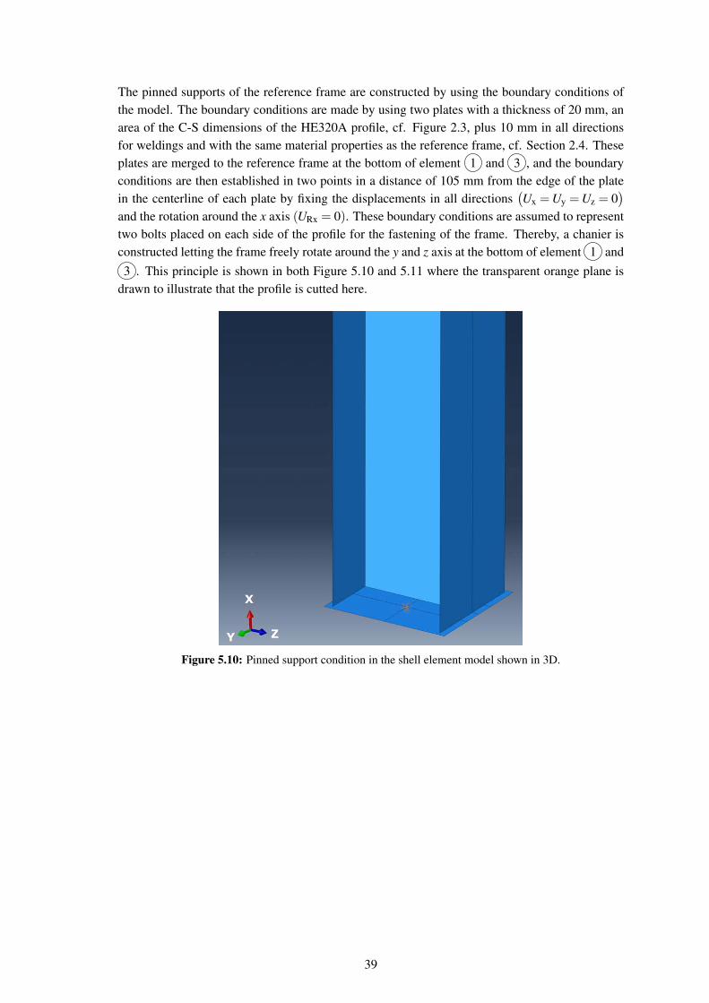
The pinned supports of the reference frame are constructed by using the boundary conditions ofthe model. The boundary conditions are made by using two plates with a thickness of 20 mm, anarea of the C-S dimensions of the HE320A profile, cf. Figure 2.3, plus 10 mm in all directionsfor weldings and with the same material properties as the reference frame, cf. Section 2.4. Theseplates are merged to the reference frame at the bottom of element 1 and 3 , and the boundaryconditions are then established in two points in a distance of 105 mm from the edge of the platein the centerline of each plate by fixing the displacements in all directions

(Ux =Uy =Uz = 0

)and the rotation around the x axis (URx = 0). These boundary conditions are assumed to representtwo bolts placed on each side of the profile for the fastening of the frame. Thereby, a chanier isconstructed letting the frame freely rotate around the y and z axis at the bottom of element 1 and3 . This principle is shown in both Figure 5.10 and 5.11 where the transparent orange plane is

drawn to illustrate that the profile is cutted here.

Figure 5.10: Pinned support condition in the shell element model shown in 3D.

39

330 mm10 mm

20 mm10 mm

320 mm

Figure 5.11: Principle sketch of plate used to make the pinned supports. The transparent orange plane isdrawn to illustrate that the profile is cutted here.

These pinned supports could also have been modelled as done with the beam elements in Section5.2.2 or by applying the boundary conditions to all the lines forming the C-S of the profile but thiswill either lead to infinitely large stresses in the area of the support or an unrealistic representationof a pinned support condition, respectively.

Boundary conditions are also established in the corners of the reference frame at the outer flangeswhere the supporting conditions are assumed to be as fork supports. Thereby, the referenceframe is fixed for out-of-plane displacement

(Uy = 0

)and for rotation around the x and z axis

(URx =URz = 0).

Loads

The uniformly distributed surface loads are applied to the frame by inflicting a pressure on theouter flanges of the frame as shown in Figure 5.12. Element 1 and 3 are, respectively,subjected to pressure and suction. The suction is modelled by a negative pressure on the outerflange of element 3 .

40

Figure 5.12: Uniformly distributed surface loads applied to the reference frame modelled by shell elementsshown in 3D.

5.3 Simulation

The Simulation step is the step where the actual numerical analysis is performed. A full analysisis conducted to get the output data which are used in the Postprocessing step to make a plot ofthe displacement in the x direction (ux) against the load exerted, q, and thereby, getting the in-plane minimum load amplifier, αult,k, by the beam element model. The out-of-plane minimumload amplifer, αcr,op, is determined by solving an eigenvalue problem which gives an eigenvaluerelated to an out-of-plane buckling mode. The eigenvalue is equal to the out-of-plane minimumload amplifier, αcr,op. An analysis in Abaqus/CAE can take from a few seconds to a couple of daysto complete depending on the complexity of model being analysed and the power of the computerused for the analysis. The Simulation step is similar for both the beam element model and theshell elemnt model. Table 5.1 shows the number of elements and nodes for each of the models.

Element modelDiscretization of Number of Number ofelement model elements nodes

Beam element model 500 60 61Shell element model 80 4465 4829

Table 5.1: Number of elements and nodes for the beam and shell element model, respectively.

As shown in Table 5.1, the shell element model is more detailed because of the larger number ofelements and nodes, and it is therefore better modelling and visualizing the effects of instabilityof the reference frame.

It is chosen to use an increment size of 0.01 and thus the loads are increased 1 % in each step. Ifthe model is not able to withstand the increase in loading, the increment size is halved and in thisway, Abaqus/CAE continues to apply the loads until the minimum increment size is reached. Thisminimum incremenet size is chosen to be 10−10.

41

5.3.1 Convergence Analysis

The level of detail of the mesh is investigated by a convergence analysis for both the beam andthe shell element model, respectively. The convergence analysis for the beam element model isshown in Figure 5.13, where it can be seen that the discretization of 500 mm is sufficient for thebeam element model to give reasonable results as the curve approximates a certain displacementwith an element length of around 500 mm.

0 50 100 150 200 250 300155

160

165

170Convergence Analysis − Beam Element Model

Number of elements

Dis

plac

emen

t, u y [m

m]

Figure 5.13: Convergence analysis for the beam element model.

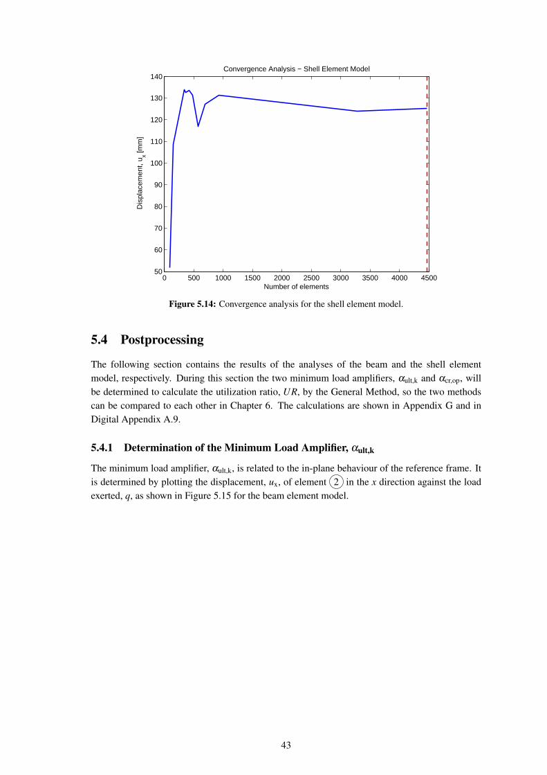
Likewise, a convergence analysis is conducted on the shell element model. This is shown in Figure5.14, whwre it can be seen that a discretization of 80 mm is sufficient for the shell element modelas well to give reasonable results.

42

0 500 1000 1500 2000 2500 3000 3500 4000 4500 50

60

70

80

90

100

110

120

130

140Convergence Analysis − Shell Element Model

Number of elements

Dis

plac

emen

t, u x [m

m]

Figure 5.14: Convergence analysis for the shell element model.

5.4 Postprocessing

The following section contains the results of the analyses of the beam and the shell elementmodel, respectively. During this section the two minimum load amplifiers, αult,k and αcr,op, willbe determined to calculate the utilization ratio, UR, by the General Method, so the two methodscan be compared to each other in Chapter 6. The calculations are shown in Appendix G and inDigital Appendix A.9.

5.4.1 Determination of the Minimum Load Amplifier, αult,k

The minimum load amplifier, αult,k, is related to the in-plane behaviour of the reference frame. Itis determined by plotting the displacement, ux, of element 2 in the x direction against the loadexerted, q, as shown in Figure 5.15 for the beam element model.

43

0 50 100 150 200 250 300 350 0

2

4

6

8

10

12Load−displacement curve − beam element model

Displacement, ux [mm]

Uni

form

line

load

, q [N

/mm

]

Load−displacement curveq

actual

qmax

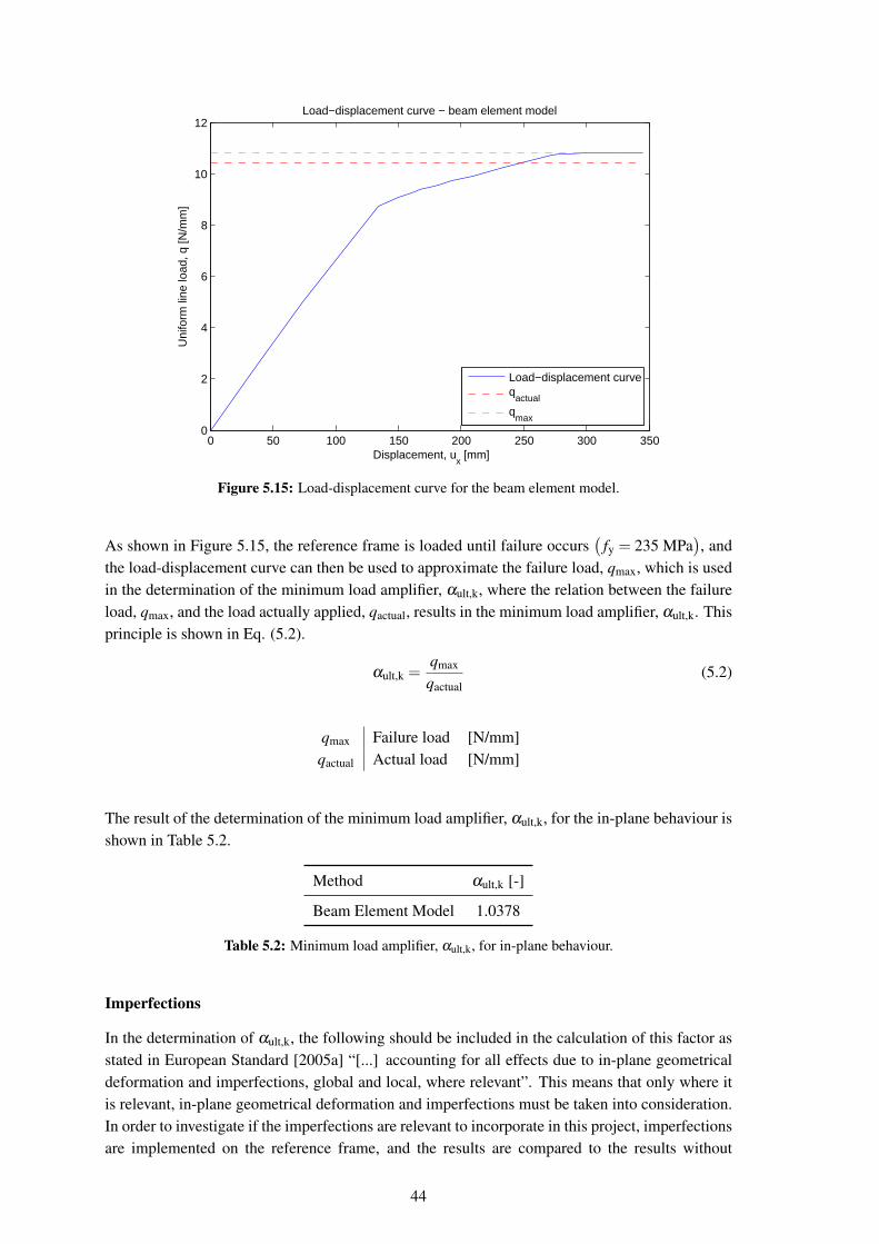
Figure 5.15: Load-displacement curve for the beam element model.

As shown in Figure 5.15, the reference frame is loaded until failure occurs(

fy = 235 MPa), and

the load-displacement curve can then be used to approximate the failure load, qmax, which is usedin the determination of the minimum load amplifier, αult,k, where the relation between the failureload, qmax, and the load actually applied, qactual, results in the minimum load amplifier, αult,k. Thisprinciple is shown in Eq. (5.2).

αult,k =qmax

qactual(5.2)

qmax Failure load [N/mm]qactual Actual load [N/mm]

The result of the determination of the minimum load amplifier, αult,k, for the in-plane behaviour isshown in Table 5.2.

Method αult,k [-]

Beam Element Model 1.0378

Table 5.2: Minimum load amplifier, αult,k, for in-plane behaviour.

Imperfections

In the determination of αult,k, the following should be included in the calculation of this factor asstated in European Standard [2005a] “[...] accounting for all effects due to in-plane geometricaldeformation and imperfections, global and local, where relevant”. This means that only where itis relevant, in-plane geometrical deformation and imperfections must be taken into consideration.In order to investigate if the imperfections are relevant to incorporate in this project, imperfectionsare implemented on the reference frame, and the results are compared to the results without

44

imperfections on the reference frame. The reference frame modelled by beam elements inAbaqus/CAE is given global initial sway imperfections and initial local bow imperfections incoherence with the recommendations from European Standard [2005a], see Appendix E. In Table5.3, the load multiplier for the maximum load on the reference frame at the yielding limit is shownfor the reference frame with and without imperfections.

Imperfections Load multiplier

None 0.010835Both sway and initial bow 0.010834Sway only 0.010834Initial bow only 0.010835

Table 5.3: Results of the load multiplier for the maximum load on the reference frame when imperfectionsare included in the beam element model.

As it can be seen in Table 5.3, the load multiplier for the maximum load of the reference frameis more or less the same whether or not imperfections are included. The displacement of thereference frame is, on the other hand, greater when imperfections are added. However, it is sothat the calculation of αult,k refers to the load amplifier, which means that the results are based onthe loads. As there is no change of maximum load at the yielding limit when imperfections areincluded, the imperfections are concluded not to be relevant for the reference frame. Hence, noimperfections are taken into account in this project report.

5.4.2 Determination of the Minimum Load Amplifier, αcr,op

The minimum load amplifier, αcr,op, is related to the out-of-plane behaviour of the referenceframe. The determination of it is based on the eigenvalue problem described in Appendix F.The eigenvalue problem is shown in Eq. (5.3). The lowest eigenvalue, λcr, giving an out-of-planebuckling mode represents the minimum load amplifier, αcr,op, since the expression in Eq. (5.4) isvalid and thereby, λcr = αcr,op.

([K]+λcr [Kσ ]ref) {δ D}= {0} (5.3)

αcr,op =qmax

qactual=

λcr qactual

qactual(5.4)

[K] Stiffness matrix [-]λcr Eigenvalue - smallest level of external load for which there is bifurcation [-]

[Kσ ]ref Stiffness matrix for stresses associated with load {R}ref [-]{δ D} Eigenvector associated with λcr is the buckling mode (shown in Abaqus) [-]

Abaqus/CAE is able to solve the eigenvalue problem in Eq. (5.3) and thereby show the lowesteigenvalue, λcr, giving an out-of-plane buckling mode. The lowest eigenvalue, λcr, is 2.8183 andthus is the minimum load amplifier, αcr,op = 2.8183 as well. It is the first buckling mode whichgives this eigenvalue, and this buckling mode is shown in Figure 5.16.

45

Figure 5.16: First buckling mode shown in 3D.

The first buckling mode shown in Figure 5.16 illustrates clearly that the reference frame bucklesout-of-the-plane and lateral torsional buckling is present.

5.4.3 Determination of the Utilization Ratio, UR

To compare the results determined by the General Method to the results determined by Method1, cf. Chapter 4, the utilization ratio, UR, is determined. This is done by the inverse of theGeneral Method as shown in Eq. (5.5). The detailed calculation by the General Method is shownin Appendix G.

UR =1

χop αult,kγM1

(5.5)

Firstly, the global non-dimensional slenderness, λ op, of a structural component for out-of-planebuckling has to be determined. This is done by the two minimum load amplifiers, αult,k and αcr,op,as shown in Eq. (5.6).

λ op =

√αult,k

αcr,op(5.6)

αult,k Minimum load amplifier for in-plane behaviour, αult,k = 1.0378 [-]αcr,op Minimum load amplifier for out-of-plane behaviour, αcr,op = 2.8183 [-]

Next, the value, ΦLT, to determine the reduction factor, χLT, for lateral torsional buckling iscalculated by Eq. (5.7).

ΦLT = 0.5[1+αLT

(λ op−λ LT,0

)+β λ

2op

](5.7)

46

αLTImperfection factor for lateral torsional buckling,

[-]αLT = 0.49 (according to buckling curve c)

λ LT,0Plateau length of the lateral torsional buckling curves

[-]for rolled sections, λ LT,0 = 0.4 (Maximum value)

βCorrection factor for the lateral torsional buckling cur-

[-]ves for rolled sections, β = 0.75 (Minimum value)

This value of ΦLT is used to determine the reduction factor, χLT, for lateral torsional buckling inEq. (5.8).

χLT =1

ΦLT +

√Φ2

LT−β λ2op

(5.8)

Hereafter, a value, Φ, to determine the reduction factor, χ , for lateral buckling is calculated in Eq.(5.9).

Φ = 0.5[1+α

(λ op−0.2

)+λ

2op

](5.9)

α Imperfection factor, α = 0.34 (according to buckling curve b) [-]

The result of Φ is used to determine the reduction factor, χ , for relevant buckling mode as shownin Eq. (5.10).

χ =1

Φ+

√Φ2−λ

2op

(5.10)

The reduction factor, χop, for the non-dimensional slenderness, λ op, can be determined by theminimum value of the reduction factor, χLT, for lateral torsional buckling and the reduction factor,χ , for lateral buckling as seen in Eq. (5.11).

χop = min

{χLT for lateral torsional buckling

χ for lateral buckling(5.11)

Finally, the utilization ratio, UR, can be determined by using Eq. (5.5), and this gives theutilization ratio, UR, shown in Table 5.4.

Model used to determine UR UR

Beam Element Model 1.3870

Table 5.4: Utilization ratios, UR, determined by the General Method

The result in Table 5.4 shows that the reference frame is utilized over 100%. In Chapter 6, theutilization ratio, UR, is compared to the utilization ratios, UR, obtained by Method 1 in Chapter4.

47

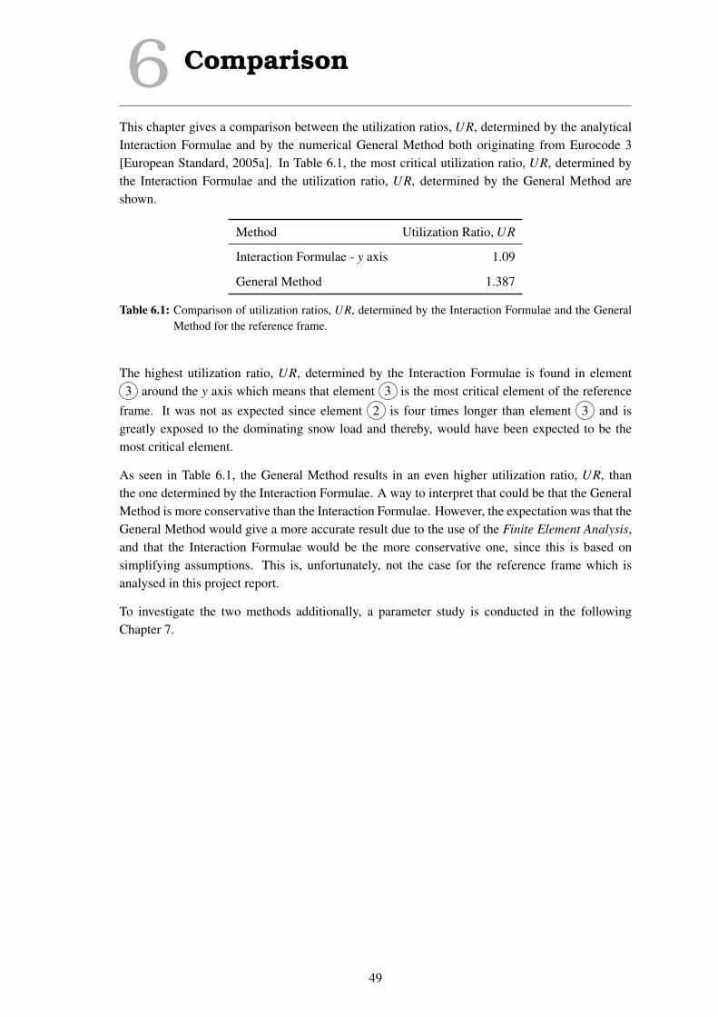
6 Comparison

This chapter gives a comparison between the utilization ratios, UR, determined by the analyticalInteraction Formulae and by the numerical General Method both originating from Eurocode 3[European Standard, 2005a]. In Table 6.1, the most critical utilization ratio, UR, determined bythe Interaction Formulae and the utilization ratio, UR, determined by the General Method areshown.

Method Utilization Ratio, UR

Interaction Formulae - y axis 1.09

General Method 1.387

Table 6.1: Comparison of utilization ratios, UR, determined by the Interaction Formulae and the GeneralMethod for the reference frame.

The highest utilization ratio, UR, determined by the Interaction Formulae is found in element3 around the y axis which means that element 3 is the most critical element of the reference

frame. It was not as expected since element 2 is four times longer than element 3 and isgreatly exposed to the dominating snow load and thereby, would have been expected to be themost critical element.

As seen in Table 6.1, the General Method results in an even higher utilization ratio, UR, thanthe one determined by the Interaction Formulae. A way to interpret that could be that the GeneralMethod is more conservative than the Interaction Formulae. However, the expectation was that theGeneral Method would give a more accurate result due to the use of the Finite Element Analysis,and that the Interaction Formulae would be the more conservative one, since this is based onsimplifying assumptions. This is, unfortunately, not the case for the reference frame which isanalysed in this project report.

To investigate the two methods additionally, a parameter study is conducted in the followingChapter 7.

49

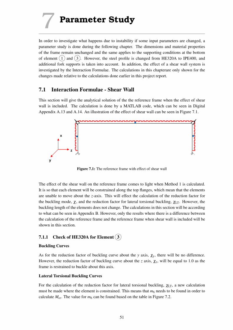
7 Parameter Study

In order to investigate what happens due to instability if some input parameters are changed, aparameter study is done during the following chapter. The dimensions and material propertiesof the frame remain unchanged and the same applies to the supporting conditions at the bottomof element 1 and 3 . However, the steel profile is changed from HE320A to IPE400, andadditional fork supports is taken into account. In addition, the effect of a shear wall system isinvestigated by the Interaction Formulae. The calculations in this chapterare only shown for thechanges made relative to the calculations done earlier in this project report.

7.1 Interaction Formulae - Shear Wall

This section will give the analytical solution of the the reference frame when the effect of shearwall is included. The calculation is done by a MATLAB code, which can be seen in DigitalAppendix A.13 and A.14. An illustration of the effect of shear wall can be seen in Figure 7.1.

z

x

y

Figure 7.1: The reference frame with effect of shear wall

The effect of the shear wall on the reference frame comes to light when Method 1 is calculated.It is so that each element will be constrained along the top flanges, which mean that the elementsare unable to move about the z-axis. This will effect the calculation of the reduction factor forthe buckling mode, χ , and the reduction factor for lateral torsional buckling, χLT. However, thebuckling length of the elements does not change. The calculations in this section will be accordingto what can be seen in Appendix B. However, only the results where there is a difference betweenthe calculation of the reference frame and the reference frame when shear wall is included will beshown in this section.

7.1.1 Check of HE320A for Element 3

Buckling Curves

As for the reduction factor of buckling curve about the y axis, χy, there will be no difference.However, the reduction factor of buckling curve about the z axis, χz, will be equal to 1.0 as theframe is restrained to buckle about this axis.

Lateral Torsional Buckling Curves

For the calculation of the reduction factor for lateral torsional buckling, χLT, a new calculationmust be made where the element is constrained. This means that m6 needs to be found in order tocalculate Mcr. The value for m6 can be found based on the table in Figure 7.2.

51

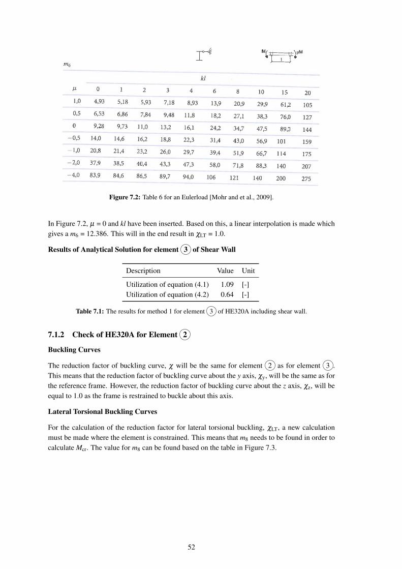
Figure 7.2: Table 6 for an Eulerload [Mohr and et al., 2009].

In Figure 7.2, µ = 0 and kl have been inserted. Based on this, a linear interpolation is made whichgives a m6 = 12.386. This will in the end result in χLT = 1.0.

Results of Analytical Solution for element 3 of Shear Wall

Description Value Unit

Utilization of equation (4.1) 1.09 [-]Utilization of equation (4.2) 0.64 [-]

Table 7.1: The results for method 1 for element 3 of HE320A including shear wall.

7.1.2 Check of HE320A for Element 2

Buckling Curves

The reduction factor of buckling curve, χ will be the same for element 2 as for element 3 .This means that the reduction factor of buckling curve about the y axis, χy, will be the same as forthe reference frame. However, the reduction factor of buckling curve about the z axis, χz, will beequal to 1.0 as the frame is restrained to buckle about this axis.

Lateral Torsional Buckling Curves

For the calculation of the reduction factor for lateral torsional buckling, χLT, a new calculationmust be made where the element is constrained. This means that m8 needs to be found in order tocalculate Mcr. The value for m8 can be found based on the table in Figure 7.3.

52

Figure 7.3: Table 8 for an Eulerload [Mohr and et al., 2009].

In order to use Figure 7.3, the two different end moments are split up and a m8 for both endmoments are calculated. The results can be seen in Table 7.2.

End moment m8 χLT

286.31 kNm 1224.0 1.0309.89 kNm 1078.53 1.0

Table 7.2: The results for the reduction factor for lateral torsional buckling, χLT.

Results of Analytical Solution for element 2 of Shear Wall

Description Value Unit

Utilization of equation (4.1) 0.87 [-]Utilization of equation (4.2) 0.49 [-]

Table 7.3: The results for method 1 for element 2 of HE320A including shear wall.

7.2 Interaction Formulae - Additional Fork Supports

This section will give the analytical solution of the the reference frame when the elements aresupported with fork supports. An illustration of the fork supports can be seen in Figure 7.4.

z

x

y

10 m

2.5 m

10 m

2.5 m

Figure 7.4: The reference frame with fork supports.

53

The effect of additional fork supports on the reference frame can be seen when the InteractionFormulae is calculated. The main effect of the additional fork supports is in regard of the thebuckling length for lateral torsional buckling. In this case, the fork supports will influencing thereduction factor for lateral torsional buckling, χLT.

The load scenario for the frame is altered from line load to point load as illustrated in Figure 7.5.The line load will in this case be concentrated at the laths and purlin, giving point loads wherethese are placed on the frame. However, the self-weight is still calculated as a line load for eachelement. It should also be noticed that the self-weight of the laths and purlin are not taken intoconsideration for this section.

64.8 kN

3.96 kN/m 3.96 kN/m

z

x

y

3.96 kN/m

32.4 kN 32.4 kN

1.65 kN

3.3 kN

0.70875 kN

1.4175 kN

1.65 kN0.70875 kN

Figure 7.5: The new loads on the frame.

The calculations in this chapter will be according to what can be seen in Appendix B. However,only the results where there is a difference between the calculation of the reference frame andthe reference frame when additional fork supports are applied is included will be shown in thissection.

7.2.1 Forces and Moments

The new load distribution on the reference frame gives the following values used in the furthercalculations, see Table 7.4.

NEd elem. 3 My,Ed elem. 3 VEd elem. 3 NEd elem. 2 My,Ed elem. 2 VEd elem. 2

136.79 kN 285.34 kNm 58.48 kN 58.48 kN 285.34 kNm 136.79 kN

Table 7.4: The new forces and moments when purlins are taken into account for the reference frame.

The new moment distribution is illustrated in Figure 7.6.

54

285.34 kNm261.75 kNm

-286.51 kNm

z

x

y

1

2

3

Figure 7.6: Illustration of the new moments occurring on the frame.

7.2.2 Check of HE320A for Element 3

Any elaboration of how the different parameters of the calculation are calculated is found inAppendix B.

Linear summation of the utilization ratios: Only one cross-section will be performed. Thischeck can be seen in Eq. (7.1) and is calculated in the following equation shown in Eq. (7.2).The reason for not taking other checks is based on the results from the previous calculations of thereference frame found in Appedix B. The experience from here shows that Eq. (7.1) is the mostcritical one.

NEd

NRd+

My,Ed

My,Rd+

Mz,Ed

Mz,Rd≤ 1.0 (7.1)

136.79 kN2515.35 kN

+285.34 kNm347.8 kNm

+0≤ 1.0 (7.2)

0.87≤ 1.0⇒ OK

For further details about the cross-section check, see Appendix B.

Buckling Curves

As for the reduction factor of buckling curve about the y axis, χy, there will be no differencefrom the reference frame as it may buckle about the same length. However, the reduction factorof buckling curve about the z axis, χz, change. The effective length will for the additional forksupports case have en effective length equal to h/2 (where h is equal to the height of the frame).When looking at the support condition for element 3 , it is assumed that when the additionalfork support is applied, the element will be fixed. Hence, the effective length is calculated for anelement with pinned and fixed supports giving ls = 0.7 · 2500 mm = 1750 mm. The effectivelength, ls = 1750 mm gives the following results shown in Table 7.5.

55

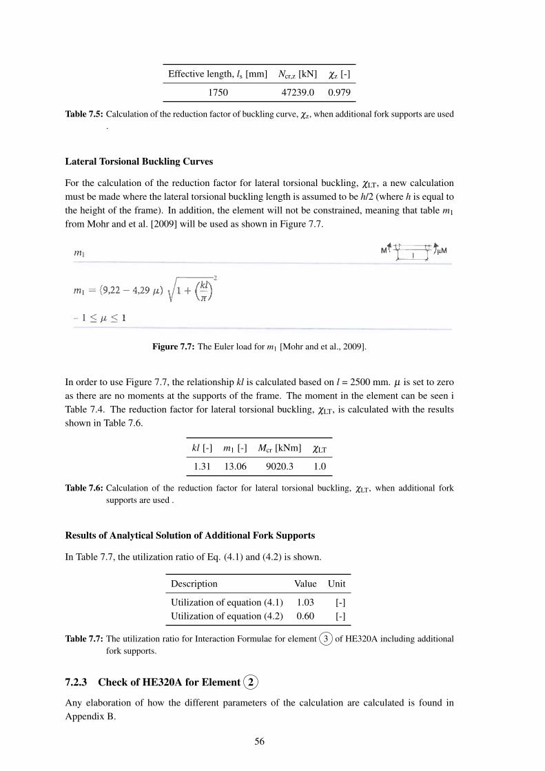
Effective length, ls [mm] Ncr,z [kN] χz [-]

1750 47239.0 0.979

Table 7.5: Calculation of the reduction factor of buckling curve, χz, when additional fork supports are used.

Lateral Torsional Buckling Curves

For the calculation of the reduction factor for lateral torsional buckling, χLT, a new calculationmust be made where the lateral torsional buckling length is assumed to be h/2 (where h is equal tothe height of the frame). In addition, the element will not be constrained, meaning that table m1

from Mohr and et al. [2009] will be used as shown in Figure 7.7.

Figure 7.7: The Euler load for m1 [Mohr and et al., 2009].

In order to use Figure 7.7, the relationship kl is calculated based on l = 2500 mm. µ is set to zeroas there are no moments at the supports of the frame. The moment in the element can be seen iTable 7.4. The reduction factor for lateral torsional buckling, χLT, is calculated with the resultsshown in Table 7.6.

kl [-] m1 [-] Mcr [kNm] χLT

1.31 13.06 9020.3 1.0

Table 7.6: Calculation of the reduction factor for lateral torsional buckling, χLT, when additional forksupports are used .

Results of Analytical Solution of Additional Fork Supports

In Table 7.7, the utilization ratio of Eq. (4.1) and (4.2) is shown.

Description Value Unit

Utilization of equation (4.1) 1.03 [-]Utilization of equation (4.2) 0.60 [-]

Table 7.7: The utilization ratio for Interaction Formulae for element 3 of HE320A including additionalfork supports.

7.2.3 Check of HE320A for Element 2

Any elaboration of how the different parameters of the calculation are calculated is found inAppendix B.

56

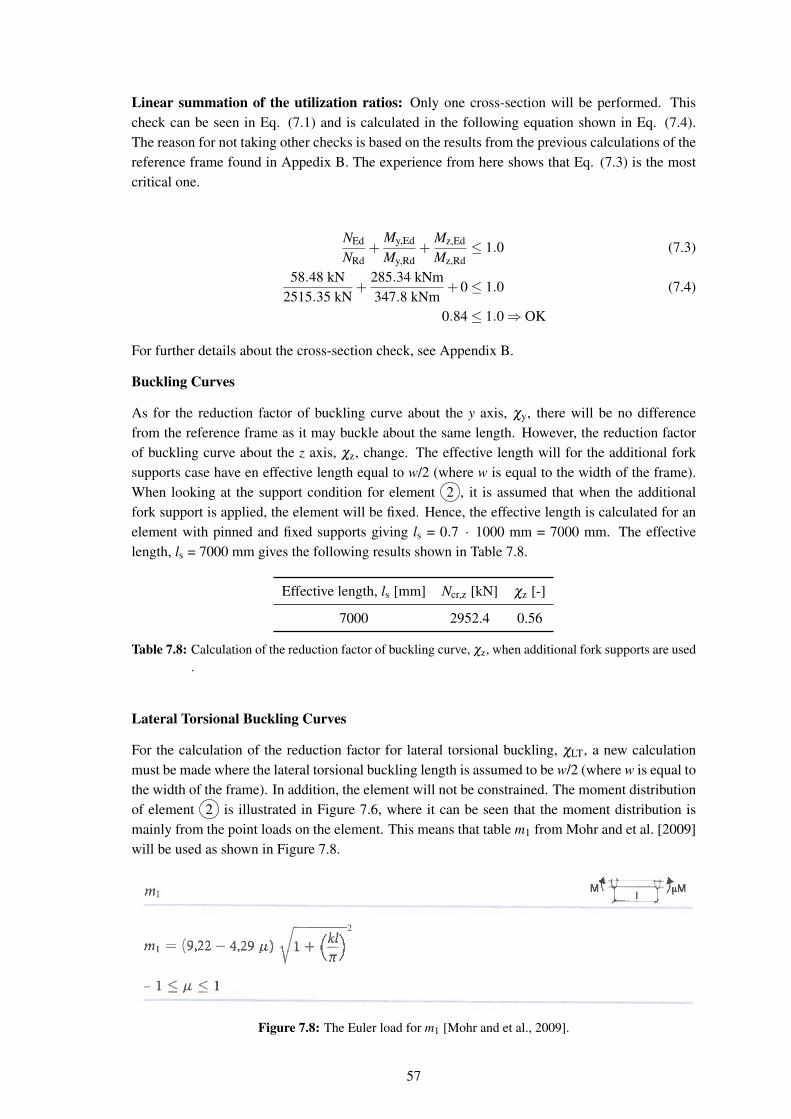
Linear summation of the utilization ratios: Only one cross-section will be performed. Thischeck can be seen in Eq. (7.1) and is calculated in the following equation shown in Eq. (7.4).The reason for not taking other checks is based on the results from the previous calculations of thereference frame found in Appedix B. The experience from here shows that Eq. (7.3) is the mostcritical one.

NEd

NRd+

My,Ed

My,Rd+

Mz,Ed

Mz,Rd≤ 1.0 (7.3)

58.48 kN2515.35 kN

+285.34 kNm347.8 kNm

+0≤ 1.0 (7.4)

0.84≤ 1.0⇒ OK

For further details about the cross-section check, see Appendix B.

Buckling Curves

As for the reduction factor of buckling curve about the y axis, χy, there will be no differencefrom the reference frame as it may buckle about the same length. However, the reduction factorof buckling curve about the z axis, χz, change. The effective length will for the additional forksupports case have en effective length equal to w/2 (where w is equal to the width of the frame).When looking at the support condition for element 2 , it is assumed that when the additionalfork support is applied, the element will be fixed. Hence, the effective length is calculated for anelement with pinned and fixed supports giving ls = 0.7 · 1000 mm = 7000 mm. The effectivelength, ls = 7000 mm gives the following results shown in Table 7.8.

Effective length, ls [mm] Ncr,z [kN] χz [-]

7000 2952.4 0.56

Table 7.8: Calculation of the reduction factor of buckling curve, χz, when additional fork supports are used.

Lateral Torsional Buckling Curves

For the calculation of the reduction factor for lateral torsional buckling, χLT, a new calculationmust be made where the lateral torsional buckling length is assumed to be w/2 (where w is equal tothe width of the frame). In addition, the element will not be constrained. The moment distributionof element 2 is illustrated in Figure 7.6, where it can be seen that the moment distribution ismainly from the point loads on the element. This means that table m1 from Mohr and et al. [2009]will be used as shown in Figure 7.8.

Figure 7.8: The Euler load for m1 [Mohr and et al., 2009].

57

In order to use Figure 7.8, the relationship kl is calculated based on l = 10000 mm. µ is calculatedfrom the relatioship of the end moment and the moment in the middle of the element, see Eq.(7.5).

µ =285.34 kNm−286.51 kNm

=−0.9959 (7.5)

By inserting µ = -0.9959 and the relationship kl, the reduction factor for lateral torsional buckling,χLT, is calculated with the results shown in Table 7.9.

kl [-] m1 [-] Mcr [kNm] χLT

5.25 22.05 951.85 0.95

Table 7.9: Calculation of the reduction factor for lateral torsional buckling, χLT, when additional forksupports are used .

Results of Analytical Solution of Additional Fork Supports

In Table 7.10, the utilization ratio of Eq. (4.1) and (4.2) is shown.

Description Value Unit

Utilization of equation (4.1) 0.85 [-]Utilization of equation (4.2) 0.49 [-]

Table 7.10: The utilization ratio for Interaction Formulae for element 2 of HE320A including additionalfork supports.

7.3 Interaction Formulae - Change of Profile to IPE500

This section will calculate the reference frame and the previously parameter study conducted forshear wall effect and additional forks supports, with a new profile, IPE500. All of the assumptionsand calculations are the same as seen in Section 4.4, 7.1 and 7.2 except for the normal force andthe moment which will be lower because of a reduction of the self-weight. This section will,however, only give the final utilization ratio for each case.

7.3.1 Reference frame - IPE

The utilization ratio for element 3 and 2 can be seen in Table 7.11 and 7.12, respectively.

Description Value Unit

Utilization of equation (4.1) 0.77 [-]Utilization of equation (4.2) 0.54 [-]

Table 7.11: The results for Interaction Formulae for element 3 of IPE500 for the reference frame.

Description Value Unit

Utilization of equation (4.1) 0.55 [-]Utilization of equation (4.2) 0.97 [-]

Table 7.12: The results for Interaction Formulae for element 2 of IPE500 for the reference frame.

58

7.3.2 Effect of Shear Wall - IPE

The utilization ratio for element 3 and 2 can be seen in Table 7.13 and 7.14, respectively.

Description Value Unit

Utilization of equation (4.1) 0.80 [-]Utilization of equation (4.2) 0.49 [-]

Table 7.13: The results for Interaction Formulae for element 3 of IPE500 for the effect of shear wall.

Description Value Unit

Utilization of equation (4.1) 0.53 [-]Utilization of equation (4.2) 0.31 [-]

Table 7.14: The results for Interaction Formulae for element 2 of IPE500 for the effect of shear wall.

7.3.3 Additional Fork Supports - IPE

The utilization ratio for element 3 and 2 can be seen in Table 7.15 and 7.16, respectively.

Description Value Unit

Utilization of equation (4.1) 0.7 [-]Utilization of equation (4.2) 0.44 [-]

Table 7.15: The results for Interaction Formulae for element 3 of IPE500 for the additional fork supports.

Description Value Unit

Utilization of equation (4.1) 0.62 [-]Utilization of equation (4.2) 0.44 [-]

Table 7.16: The results for Interaction Formulae for element 2 of IPE500 for the the additional forksupports.

7.4 General Method - Shear Wall

The reference frame is in this section modified to the configuration shown in Figure 7.9, wherean effect of a shear wall system is present. A purlin is placed on the upper flange on element 2while laths are placed on the outer flanges on element 1 and 3 , respectively. These out-of-plane elements are used as supports for the cladding and to stabilize the frame out-of-the-plane.

59

z

x

y

Figure 7.9: Effect of shear wall system.

To model this configuration in Abaqus/CAE, the boundary conditions and loads are changedcompared to what is done on the reference frame. The pinned support conditions and the forksupports in the corners of the frame are still applied but now the frame is out-of-plane supportedat the midpoints of the elements. This means that in these points Uy = 0. Additionally, the rotationaround the z axis, URz, is fixed and thereby equal to zero at the midpoints of element 1 and 3while the rotation around the x axis, URx, is fixed and thereby equal to zero at the midpoint ofelement 2 . Because of these out-of-plane elements, the loading conditions are changed fromuniformly distributed surface loads acting on the outer flanges to point loads acting at the pinnedsupports, the midpoints and the corners of the frame. The loads are shown in Figure 7.5.

The General Method is used to determine the utilization ratio, UR, of this configuration. TheGeneral Method is described in Chapter 5 and a worked example is shown in Appendix G. Theresults of an analysis of this configuration are shown in Table 7.17.

Description Symbol Value Unit

Minimum load amplifier related to in-plane behaviour αult,k 0.6757 [-]Minimum load amplifier related to out-of-plane behaviour αcr,op 1.4975 [-]Utilization ratio UR 2.2215 [-]

Table 7.17: Minimum load amplifiers, αult,k and αcr,op, related to in-plane and out-of-plane behaviour,respectively, and utilization ratio, UR, for frame with effect of shear wall system.

As seen in Table 7.17, this configuration results in an even larger utilization ratio, UR, than thereference frame. Therefore, there must be an error somewhere, since this configuration should bemore stable and thereby less utilized than the reference frame.

7.5 Discussion

From the analytical parameter study conducted, the worst case for an element with HE320A profileturned out to be the reference frame and the reference frame when shear wall is included. Thehighest utilization ratio was 1.09 (109 %) for element 3 . The reason for the worst case beingboth the reference frame and the reference frame when shear wall is included is due to the criticalmoment, Mcr. The critical moment will result in a reduction factor for lateral torsional buckling,χLT of 1.0 for both cases. For the General Method, the effect of shear wall gave a utilizationratio of 2.22 (222%), which is significantly higher than expected. It would be assumed that theanalytical method would be more conservative, and that the General Method would give the lowestutilization ratio due to the use of Finite Element Analysis.

60

In regard of the parameter study for an element with IPE 500 profile, the worst case is for thereference frame about the z axis for element 2 . This is most likely due to sectional propertiesabout the z axis, meaning that for an element length of 20 m, the z axis will become critical.

For the analytical parameter study it can be said that the reference frame will for all cases be themost critical by having the highest utilization ratio. As the elements are supported by additionalfork supports, the utilization ratio decrease as suspected.

61

8 Conclusion

The goal of this master thesis has been to investigate a predefined reference frame for instabilityby two different methods given in Eurocode 3 [European Standard, 2005a]. The first one - theInteraction Formulae - determines directly the utilization ratio, UR, of an element subjectedto combined bending and axial compression around both the y and z axis. The method takesinto account instability effects such as buckling and lateral torsional buckling, and it is highlydependent on how the supporting conditions are assumed.

The Interaction Formulae shows a utilization ratio, UR, of 1.09 (109%) around the y axis ofelement 3 . This means that for the reference frame, element 3 will be the critical element.The results shows that buckling effects are critical due to the slenderness of the section. However,lateral torsional buckling effects are not critical for this element.

The second method to investigate a frame for instability is the General Method which allows tomake use of a Finite Element Analysis to determine two minimum load amplifiers, αult,k and αcr,op,related to the in-plane and out-of-plane behaviour of a frame, respectively. The utilization ratio,UR, determined by the General Method is unfortunately higher than the one determined by theInteraction Formulae. The General Method results in a utilization ratio, UR, of 1.3870 (139%).

A way to interpret that the utilization ratio, UR, is higher determined by the General Methodcompared to the Interaction Formulae could be that the General Method is more conservativethan the Interaction Formulae. However, the expectation was that the General Method wouldgive a more accurate result due to the use of the Finite Element Analysis, and that the InteractionFormulae would be the more conservative one, since this is based on simplifying assumptions.This is, unfortunately, not the case for the reference frame which is analysed in this master thesis.In the parameter study for the Interaction Formulae, the utilization ratio of element 2 is found tobe the worst case with a value of 0.97 (97%) about the z axis for the reference frame by using anIPE500 steel profile. It can aslo be seen from the parameter study that the additional fork supportson the frame will help to stabilize and in the end giving a smaller utilization ratio for the frame.

8.1 Further Studies

There are a number of different parameters which are well suited for an analysis of a frame, butbecause of the extent and complexity of frame, only some parameters has been chosen. However,there are further studies that can be made in order to investigate a steel frame. Some of thesefurther studies are listed below:

• In a further investigation of a steel frame, the support conditions could be altered to fixedsupports to see what effect that would have on the stability of the frame by using the Inter-action Formulae and the General Method.

• The angle of the roof could have been varied in order to investigate how a pitched-roofframe would behave according to the Interaction Formulae and the General Method.

• From the literature study, articles shows that the stability of the frame is very depending onhow the joints of the frame is modeled. This will have a great impact on the stability of theframe, and it would therefore be interesting to investigate further.

63

• The cross-section of the frame could be made with a non constant cross-section in order tosee how the General Method would analyse the stability the frame.

64

Bibliography

Andersen and Petersen, 2010. Ulrik Andersen and Stefan Petersen. Bygningsingeniør:Halvdelen af undersøgte tage har fejl - 6.000 tage bør tjekkes. URL:http://kortlink.dk/c3q7, 2010. Downloaded: 15-02-2013.

Autobaler. Autobaler. Portal Frame Buildings. URL: http://kortlink.dk/cewp.Downloaded: 05-04-2013.

Bonnerup and et al., 2009. Bent Bonnerup and et al. Stålkonstruktioner efter DS/EN 1993. NytTeknisk Forlag, 1. edition, 2009. ISBN 978-87-571-2683-9.

BYG-ERFA. BYG-ERFA. Forstærkning af simple stålrammebygninger. URL:https://kortlink.dk/a99e. Downloaded: 04-04-2013.

Connections.org. Connections.org. Flexural-Torsional Buckling. URL:http://kortlink.dk/cews. Downloaded: 13-05-2013.

Silva and et al, 2010. Luís Simões da Silva and et al. Design of Steel Structures, Eurocode 3:Design of steel structures. Part 1-1: General rules and rules for buildings. ECCS - EuropeanConvention for Constructional Steelwork, 2010.

Eurocode-resources.com. Eurocode-resources.com. Buckling. URL:http://kortlink.dk/cewn. Downloaded: 04-04-2013.

European Standard, 2005a. European Standard. Eurocode 3: Design of Steel Structures - Part1-1: General Rules and Rules for Buildings. European Standard, 2005.

European Standard, 2005b. European Standard. Eurocode 0: Basic of Structural Design.European Standard, 2005.

European Standard, 2002. European Standard. Eurocode 1: Actions on structures - Part 1-1:General actions - Densities, self-weight, imposed loads for buildings. European Standard,2002.

European Standard, 2007a. European Standard. Eurocode 1: Actions on structures - Part 1-3:General actions - Snow loads. European Standard, 2007.

European Standard, 2007b. European Standard. Eurocode 1: Actions on structures - Part 1-4:General actions - Wind actions. European Standard, 2007.

Freedom Steel, 2010. Freedom Steel. URL: http://kortlink.dk/chfm, 2010. Downloaded:02-06-2013.

Lett-Tak Systemer AS. Lett-Tak Systemer AS. Lett-Tak. URL: http://kortlink.dk/cewg.Downloaded: 06-05-2013.

Ljubljana University, a. Ljubljana University. Lecture 6.3: Elastic Instability Modes. URL:http://kortlink.dk/cewm. Downloaded: 04-04-2013.

Ljubljana University, b. Ljubljana University. Lecture 6.6.2: Buckling of Real Structural,Elements II. URL: http://kortlink.dk/cewk. Downloaded: 04-04-2013.

Made-in-China.com. Made-in-China.com. URL: http://kortlink.dk/chfn. Downloaded:02-06-2013.

65

Mohr and et al., 2009. Gunnar Mohr and et al. Teknisk Ståbi. Nyt Teknisk Forlag, 20. edition,2009. ISBN 978-87-571-2685-3.

SIMULIA, 2012. SIMULIA. Getting Started with Abaqus: Interactive Edition, 2012.

Solberg, 2011. Andreas Solberg. Historiske kollapser de siste 10 år. URL:http://kortlink.dk/c3q6, 2011. Downloaded: 15-02-2013.

Steltech-Structural. Steltech-Structural. Portal Frame Buildings. URL:http://kortlink.dk/cewq. Downloaded: 05-04-2013.

Wikipedia. Wikipedia. Column. URL: http://kortlink.dk/cewr. Downloaded:16-04-2013.

66