Embed Size (px)
Citation preview

A 111 D 2
Bureau of StenM™
>
hmiffiffstandards & tech R|c -
2 2A970
3C100 U573 V33;1 970 C.1 NBS-PUB-C 1964
°r cCv
7>r X'd1 \
0 r. >^ns o* *
NBS
PUBLICATIONS
NSRDS—NBS 33
NSRDS
Electrolytic Conductance
And the Conductances of the
Halogen Acids in Water
u.s.
DEPARTMENTOF
COMMERCENational
n—jureaijof
idards>jn3m\oo
r\jo
iqiO
sdjbi
ozbi
•spiflJQTl
jBDU^iS 1° nesiftfl puo^Mi
NATIONAL BUREAU OF STANDARDS
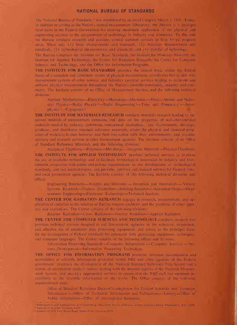
The National Bureau of Standards 1 was established by an act of Congress March 3, 1901. Today,
in addition to serving as the Nation’s central measurement laboratory, the Bureau is a principal
focal point in the Federal Government for assuring maximum application of the physical and
engineering sciences to the advancement of technology in industry and commerce. To this end
the Bureau conducts research and provides central national services in four broad program
areas. These are: (1) basic measurements and standards, (2) materials measurements and
standards, (3) technological measurements and standards, and (4) transfer of technology.
The Bureau comprises the Institute for Basic Standards, the Institute for Materials Research, the
Institute for Applied Technology, the Center for Radiation Research, the Center for Computer
Sciences and Technology, and the Office for Information Programs.
THE INSTITUTE FOR BASIC STANDARDS provides the central basis within the United
States of a complete and consistent system of physical measurement; coordinates that system with
measurement systems of other nations; and furnishes essential services leading to accurate and
uniform physical measurements throughout the Nation’s scientific community, industry, and com-
merce. The Institute consists of an Office of Measurement Services and the following technical
divisions:
Applied Mathematics—Electricity—Metrology—Mechanics—Heat—Atomic and Molec-
ular Physics—Radio Physics -—Radio Engineering -—Time and Frequency -—Astro-
physics -—Cryogenics.-
THE INSTITUTE FOR MATERIALS RESEARCH conducts materials research leading to im-
proved methods of measurement standards, and data on the properties of well-characterized
materials needed by industry, commerce, educational institutions, and Government; develops,
produces, and distributes standard reference materials; relates the physical and chemical prop-
erties of materials to their behavior and their interaction with their environments; and provides
advisory and research services to other Government agencies. The Institute consists of an Office
of Standard Reference Materials and the following divisions:
Analytical Chemistry—Polymers—Metallurgy—Inorganic Materials—Physical Chemistry.
THE INSTITUTE FOR APPLIED TECHNOLOGY provides technical services to promote
the use of available technology and to facilitate technological innovation in industry and Gov-
ernment; cooperates with public and private organizations in the development of technological
standards, and test methodologies; and provides advisory and research services for Federal, state,
and local government agencies. The Institute consists of the following technical divisions and
offices:
Engineering Standards—Weights and Measures— Invention and Innovation — Vehicle
Systems Research—Product Evaluation—Building Research—Instrument Shops—Meas-
urement Engineering—Electronic Technology—Technical Analysis.
THE CENTER FOR RADIATION RESEARCH engages in research, measurement, and ap-
plication of radiation to the solution of Bureau mission problems and the problems of other agen-
cies and institutions. The Center consists of the following divisions:
Reactor Radiation—Linac Radiation—Nuclear Radiation—Applied Radiation.
THE CENTER FOR COMPUTER SCIENCES AND TECHNOLOGY conducts research and•
provides technical services designed to aid Government agencies in the selection, acquisition,
and effective use of automatic data processing equipment; and serves as the principal focus
for the development of Federal standards for automatic data processing equipment, techniques,
and computer languages. The Center consists of the following offices and divisions:
Information Processing Standards—Computer Information — Computer Services— Sys-
tems Development—Information Processing Technology.
THE OFFICE FOR INFORMATION PROGRAMS promotes optimum dissemination and
accessibility of scientific information generated within NBS and other agencies of the Federal
government; promotes the development of the National Standard Reference Data System and a
system of information analysis centers dealing with the broader aspects of the National Measure-
ment System, and provides appropriate services to ensure that the NBS staff has optimum ac-
cessibility to the scientific information of the world. The Office consists of the following
organizational units:
Office of Standard Reference Data—Clearinghouse for Federal Scientific and Technical
Information *—Office of Technical Information and Publications—Library—Office of
Public Information—Office of International Relations.
1 Headquarters and Laboratories at Gaithersburg:, Maryland, unless otherwise noted; mailing address Washington, D.C. 20234.- Located at Boulder. Colorado 80302.
Located at 5285 Port Royal Road, Springfield, Virginia 22151.

UNITED STATES DEPARTMENT OF COMMERCE
Maurice H. Stans, Secretary,
NATIONAL BUREAU OF STANDARDS# Lewis M. Branscomb, DirectorI « I
Electrolytic Conductance and the Conductances of the
Halogen Acids in Water
Walter J. Hamer and Harold J. DeWane
Institute for Basic Standards
National Bureau of Standards
Washington, D.C. 20234
NSRDS
NSRDS-NBS 33
Nat. Stand. Ref. Data Ser., Nat. Bur. Stand. (U.S.), 33, 37 pages (May 1970) CODEN: NSRDA
Issued May 1970
For sale by the Superintendent of Documents, U.S. Government Printing Office, Washington, D.C. 20402
(Order by SD Catalog No. C 13.48:33), Price 5U cents

NATIONAL BUREAU OF STANDARDS
JUL 2 3 1S70
QC/O n
US 73
DO,Foreword
j
The National Standard Reference Data System provides effective access to the quantitative
data of physical science, critically evaluated and compiled for convenience, and readily accessible
through a variety of distribution channels. The System was established in 1963 by action of the
President’s Office of Science and Technology and the Federal Council for Science and Tech-
nology, with responsibility to administer it assigned to the National Bureau of Standards.
The System now comprises a complex of data centers and other activities, carried on in aca-
demic institutions and other laboratories both in and out of government. The independent opera-
tional status of existing critical data projects is maintained and encouraged. Data centers that
are components of the NSRDS produce compilations of critically evaluated data, critical reviews
of the state of quantitative knowledge in specialized areas, and computations of useful functions
derived from standard reference data. In addition, the centers and projects establish criteria
for evaluation and compilation of data and make recommendations on needed improvements in
experimental techniques. They are normally closely associated with active research in the relevant
field.
The technical scope of the NSRDS is indicated by the principal categories of data compilation
projects now active or being planned: nuclear properties, atomic and molecular properties, solid
state properties, thermodynamic and transport properties, chemical kinetics, and colloid and
surface properties.
The NSRDS receives advice and planning assistance from the National Research Council
of the National Academy of Sciences-National Academy of Engineering. An overall Review Com-
mittee considers the program as a whole and makes recommendations on policy, long-term plan-
ning, and international collaboration. Advisory Panels, each concerned with a single technical
area, meet regularly to examine major portions of the program, assign relative priorities, and
identify specific key problems in need of further attention. For selected specific topics, the Advisory
Panels sponsor subpanels which make detailed studies of users’ needs, the present state of knowl-
edge, and existing data resources as a basis for recommending one or more data compilation
activities. This assembly of advisory services contributes greatly to the guidance of NSRDSactivities.
The NSRDS-NBS series of publications is intended primarily to include evaluated reference
data and critical reviews of long-term interest to the scientific and technical community.
Lewis M. Branscomb, Director
© 1970 by the Secretary of Commerce on behalf of the United States Government.
Library of Congress Catalog Card Number: 79-604209
II

Preface
This document represents the initial effort in the compilation and critical evaluation of avail-
able data on the electrolytic conductance of aqueous solutions of electrolytes. A readily available
source of such data is presently needed since the last such compilation and evaluation was madein the early 1930’s. Although, for the most part, these data are available in the literature, they
have not been brought together in a single volume nor have they been treated in a consistent
manner. For example, some data in the literature are given in international ohms, others in absolute
ohms. Methods used to obtain limiting equivalent conductances differ widely. Also most of the
literature data are expressed on the old atomic weight scale of 16 for naturally occurring oxygen
rather than on the 12C scale. All data reported here have been converted to absolute ohms, and
the 12C scale of atomic weights; data presented in subsequent reports will be treated in a similar
manner.
Modern theories of conductance, especially those developed by Peter J. W. Debye, Lars
Onsager, and Raymond M. Fuoss are or will be used in the critical evaluation of the data, in par-
ticular for the determination of limiting equivalent conductances. Also when the available data
are of sufficient accuracy, modern theories will be used to determine apparent “ion-size” param-
eters; such determinations will not be made in the present document, however. In general, the
data on equivalent conductances will be presented in tables. Equations, based in part on theory,
which give equivalent conductances as a function of concentration will also be included. In some
cases, empirical equations will be used in the entirety, but these will reproduce the experimental
results which are, in essence, the essential product desired by the user. For example, empirical
equations are used to express the conductances of HC1 at —10 and —20 °C; in the limit of zero
concentration the solutions are solid, i.e., in the frozen state.
In the present document, definitions relating to the conductance of electrolytic solutions
are first presented. These are followed by some general considerations of the migration of ions
and general laws governing the movement of ions under applied potential gradients as are in-
volved in electrolytic conductance. Conductance relations (equations) are then given, and these
are followed by a condensed treatment of the Debye-Hiickel-Onsager-Fuoss theories of electrolytic
conductance, given in general terms (a more detailed treatment is given in Appendix A, but even
there the minor details and mathematical complexities are omitted). Values of the parameters,
namely B i, B 2 , E\, and E 2 in the theoretical equations are given for temperatures from 0 to 100 °C
for the convenience of those engaged in conductance measurements. They are not needed, how-
ever, by those who are interested only in data on the equivalent conductance of an electrolytic
solution. Finally, tables of data on the electrolytic conductance of HF, HC1, HBr, and HI are given
for various concentrations and temperatures in tables 10 through 19. The constants governing the
dissociation of HF from 0 to 25 °C are given in table 9.
Ill

For the convenience of the reader a glossary of symbols is given at the end of the document.
In 1968, the Commission on Symbols, Terminology, and Units of the Division of Physical
Chemistry of the International Union of Pure and Applied Chemistry in a tentative proposal
(IUPAC Bulletin No. 32) did not include “equivalent conductance” among its list of definitions,
but replaced it by “molar conductance” and assigned the symbol A to the latter. Accordingly, if
this proposal is eventually adopted, the term “equivalent” in the present document should be
replaced by “molar” and the definitions of “molar conductance” and “limiting molar conductance”
given on page 1 eliminated (historically, molar conductivity, as defined on page 1, had use in deter-
mining the mode of ionization of salts when it was not possible to determine the equivalent weight
of the salt). Under this proposal of IUPAC, the meaning of a mole of salt would need to be clearly
specified. Thus, the molar conductance of MgCU, for example, could be given as
A(£ MgCl2)= 129 a- 1 cm 2mol-1 or as A(MgCl 2 )= 258 D _1 cm 2 mol_1
(see IUPAC Bulletin No. 32) depending on how a mole of MgCU is specified (of course, Avogadro’s
constant would apply only to the latter definition).
Acknowledgment
The authors wish to express their appreciation to Professor Raymond M. Fuoss of Yale Uni-
versity for his advice during the course of this work.
IV

Contents
Page
Foreword II
Preface Ill
1. Definitions and symbols 1
2. General considerations 3
3. General laws . 3
4. Conductance relations 4
5. Theoretical expressions for equivalent conductance... 5
6. Determination of Ao 8
7. Equivalent conductances of HF, HC1, HBr, HI 8
HF 8
HC1 10
HBr 12
HI 12
8. Conclusions 13
9. References 13
10. Appendix A. The Debye-Hiickel-Onsager-Fuoss
theory of electrolytic conductance 14
A. Bibliography for Appendix A 18
11. Appendix B. Densities of aqueous solutions of HF 18
12. Appendix C. Use of the Systeme International
d'Unites 19
13. Tables •. 19
Table 1. Specific conductances of standard aqueous
solutions of KC1 19
Table 2. Physical properties of water 20
Table 3. Values of the Debye-Hiickel-Onsager con-
stants B i and B 2 for equivalent conductances for
1-1 aqueous solutions from 0 to 100 °C 20
Table 4. Values of the Fuoss-Onsager E\ and E2
constants for equivalent conductances for
1-1 aqueous solutions from 0 to 100 °C 21
Table 5. Differences in the values of B t and B2
from those given in table 3 if the dielectric
constants of water determined by Owen et al.
Page
are used instead of those of Malmberg and
Maryott 21
Table 6. Differences in the values of E\ and E2
from those given in table 4 if the dielectric
constants of water determined by Owen et al.
are used instead of those of Malmberg and
Maryott 22
Table 7. Values of the Debye-Hiickel constants
A c and Bc for activity coefficients of aqueous
solutions from 0 to 100 °C 22
Table 8. Values of A0 for HF 23
Table 9. Values of the constants governing the
dissociation of HF 23
Table 10. Equivalent conductances of aqueous
solutions of HF at 0, 16, 18, 20, and 25 °C 23
Table 11. Equivalent conductances of aqueous
solutions of HC1 from —20 to 65 °C 24
Table 12. Interpolation equations, constants,
and coefficients for A for HC1 25
Table 13. Equivalent conductances of aqueous
solutions of HBr at 25 °C 26
Table 14. Equivalent conductances of aqueous
solutions of HBr from —20 to 50 °C 27Table 15. Interpolation equations, constants,
coefficients, and standard deviations of fits
for A for HBr 28
Table 16. Equivalent conductances of aqueous
solutions of HI at 25 °C 29
Table 17. Equivalent conductances of aqueous
solutions of HI from — 20 to 50 Tl 30
Table 18. Interpolation formulas for A for HI 31
Table 19. Limiting equivalent conductances of
HF, HC1, HBr, and HI in water at 25 °C 31
14.
Glossary of symbols 32
V

— , I
ss

Electrolytic Conductance and the Conductances of the
Halogen Acids in Water
Walter J. Hamer and Harold J. DeWane
Definitions, symbols, general principles, and general laws related to the electrolytic conductanceof aqueous solutions are presented. The general laws considered are Coulomb’s law for chargedbodies, Poisson’s equation relating the electrostatic potential to charge distribution, and the Stokes andOseen laws for the velocity of a sphere in a fluid medium. The relations between electrical resistance,
electrical conductance, specific resistance, specific conductance, and equivalent conductance are
set forth. Theoretical expressions for the equivalent conductance as derived by Debye, Onsager, andFuoss are given in general form and in a somewhat more detailed fashion in an appendix. The general
methods of treating the equivalent conductances of ionophores and ionogens, especially in regard
to the determination of the limiting equivalent conductance, the degree of ionic association, and the
degree of ionic dissociation are discussed. Data on the equivalent conductances of the halogen acids,
hydrofluoric, hydrochloric, hydrobromic, and hydriodic acids in water are given for a wide range of
concentration and temperature.
Key words: Conductances of HF, HC1, HBr, and HI; electrolytic conductance; theories ot electrolytic
conductance.
1. Definitions and Symbols
Conductance, cr — The conductance of a conductorof electricity is the reciprocal of its electrical
resistance (R ) and its unit is the reciprocal “ab-
solute” ohm, ohm-1, or mho.
Specific conductance, crsp— The specific con-
ductance, or conductivity, of a conductor of elec-
tricity is the conductance of the material betweenopposite sides of a cube, one centimeter in eachdirection. The unit of specific conductance is
ohm -1 cm-1or mho cm -1
.
Electrolytic cell constant, Jc — The cell constant
of an electrolytic cell is the resistance in ohmsof that cell when filled with a liquid of unit re-
sistance.
Equivalent conductance. A— The equivalent
conductance of an electrolytic solution is the
conductance of the amount of solution that con-
tains one gram-equivalent of a solute (or electro-
lyte) when measured between parallel electrodes
which are one centimeter apart and large enoughin area to include the necessary volume of solution.
Equivalent conductance is numerically equalto the conductivity multiplied by the volume in
cubic centimeters containing one gram-equivalentof the electrolyte. The unit of equivalent conduct-ance is ohm -1 cm2 equiv -1
(frequently, in the
literature the unit is given simply, although in-
correctly, as ohm -1, so that it may be comparable
to the unit for conductance, in general).
Limiting equivalent conductance, Ao— Thelimiting equivalent conductance of an electrolytic
solution, Ao, is expressed by Ao=lim ( a-C0rJc
)
where (Ton. is solution conductance corrected for
solvent conductance and c is the equivalent con-
centration. Ao is the value which A approachesas the solution is diluted so far that the effects
of interionic forces become negligible (and dis-
sociation, in the case of ionogens, is essentially
complete).
Molar conductance, Aw— The molar conductanceof an electrolytic solution is the conductanceof a solution containing one gram mole of the solute
(or electrolyte) when measured in a like manner to
equivalent conductance. Seldomly used.
Limiting molar conductance, A^— The limiting
molar conductance of an electrolytic solution,
A(,”, is expressed by Ag'^lim (o-C0rr/m) where
<xcorr is solution conductance corrected for solvent
conductance and m is the molar concentration.
A^ is the value which Am approaches as the solution
is diluted so far that the effects of interionic forces
become negligible. Seldomly used.
Degree of dissociation (or ionization) in general,
a— The degree of dissociation (or ionization) of
an electrolytic solution is the percentage of solute
(or electrolyte) in the dissociated (or ionized)
state in solution. Classically this degree is obtainedfrom conductance measurements from the ratio,
A/A i where A; is the equivalent conductance anelectrolytic solution would have at some finite
concentration if it were completely dissociated
into ions at that concentration. (See ionogens).
This symbol is also used to denote the fraction
of free ions in a solution when simple ions, ion
pairs, and clusters higher than ion pairs are present.
(See ionophores).
Degree of association, (1— a) — The degree of
association of an electrolytic solution is the per-
centage of ions associated into nonconductingspecies, such as ion-pairs. (See ionophores).
Ionic equivalent conductance, The ionic
equivalent conductance is the equivalent conduct-ance of an individual ion constituent of the solute
(or electrolyte) of an electrolytic solution. This
1

symbol is also used to designate the equivalentconductance of complex ions, ion pairs, ion clusters,
etc., in combination with simple ions.
Limiting ionic equivalent conductance, \o— Thelimiting ionic equivalent conductance of an individ-
ual ion constituent of the solute (or electrolyte) of anelectrolytic solution is given by A.0 = lim (A/c). This
c —>0symbol is also used to designate the limiting
equivalent conductances of complex ions, ion
pairs, ion clusters, etc., in combination withsimple ions.
Ionic mobility, a— The mobility of an ion at anyfinite equivalent concentration is the velocity
with which the ion moves under unit potential
gradient. Its unit is cm2 sec -1volt
-1 equiv-1 or
cm2 ohm-1 F-1 where F is the Faraday expressedin coulombs (or ampere seconds) equiv -1
.
Limiting ionic mobility, a0 — The limiting mobility
of an individual ion of a solute (or electrolyte) is
given by u° =lim u.c—»0
Kohlrausch law of independent migration ofions — The value of the equivalent conductance,as the concentration approaches zero, is equal to
the sum of the limiting ionic equivalent conduct-ances of the ions constituting the solute of the
electrolytic solution.
Transference (or transport) number, t— Thetransference number of each ion of a solute (or
electrolyte) in an electrolytic solution is the fraction
of the total current carried by that ion, and is givenby the ratio of the mobility of the ion to the sum of
the mobilities of the ions of the solute constituting
the electrolytic solution.
Interionic attraction— The electrostatic attrac-
tion between ions of unlike charge (sign).
Interionic repulsion — The electrostatic repulsionbetween ions of like charge (sign).
Ion atmosphere (or continuous charge distribu-
tion)— In the electrostatic effects between ions theterm ion atmosphere denotes a continuous chargedistribution, or charge density, p (r), which is a
continuous function of r, the distance from thereference ion, rather than a discrete or discon-
tinuous charge distribution. The ion atmosphereextends from r—a to r— 0(Vlls
)~ °°, where V is the
volume of the system, and acts electrostatically
somewhat like a sphere of charge — e at a distance,k- 1
, from the reference ion of charge -fie (see belowfor definition of k -1
).
Thickness or average radius of ion atmosphere,k- 1 — The average distance of the ion atmosphere
from the reference ion in angstrom units. Thisaverage distance decreases in magnitude with thesquare root of the ionic concentration. Mathe-matically, /c
-1is the distance at which the average
charge, dq, in a spherical shell of volume 4>nr2drreaches a maximum using the continuous density,
p (r), approximation.
Ion size or “ion-size” parameter, a (or a,) — Theion size is formally considered to be the sum ofthe ionic radii of the oppositely charged ions
in contact. The ion size is also called the “distanceof closest approach” of the ions, or the “ion-size”
parameter. Generally the ion size is greater than the
sum of the crystal radii, and the “ion-size” param-eter may include several factors which contribute
to its numerical value.
Electrophoretic effect— The slowing down, owingto interionic attraction and repulsion, of the move-ment of an ion with its solvent molecules in the
forward direction by ions of opposite charge with
their solvent molecules moving in the reverse
direction under an applied electrical field (po-
tential gradient).
Relaxation-field effect— The delay in the ion
atmosphere in maintaining its symmetry arounda central ion as the central ion moves in the for-
ward direction under an applied electrical field
(potential gradient).
Osmotic-pressure effect— An enhancement in
the velocity of the central ion, in the direction
of the applied external field, as a result of morecollisions on the central ion from ions behind the
central ion than from ions in front of it.
Viscosity effect— An alteration in the velocity
of a given ion as a result of the contribution to the
bulk viscosity owing to the ions of opposite charge.
This effect applies to ions of large size.
Walden’s rule, A0170— Walden’s rule states that
the product of the limiting equivalent conductanceof an electrolytic solution, A0 ,
and the viscosity of
the solvent, 170, in which the solute (or electrolyte)
is dissolved is a constant at a particular tempera-
ture. Walden’s rule is an approximation whichwould be valid only for ions which behave hydro-
dynamically like Stokes spheres in a continiuum
(see later for Stokes Law).
Debye-Falkenhagen effect— The increase in the
conductance of an electrolytic solution producedby alternating currents of sufficiently high fre-
quencies over that observed with low frequencies
or with direct current.
Wien effect— The increase in the conductance of
an electrolytic solution produced by high electrical
fields (potential gradients).
Dissociation-field effect— The increased dissocia-
tion (or ionization) of the molecules of weak elec-
trolytes under the influence of high electrical fields
(potential gradients).
Ionophores— Substances, like sodium chloride,
which exist only as ionic lattices in the pure crystal-
line form, and which when dissolved in an appro-
priate solvent give conductances which changeaccording to some fractional power of the concen-tration. Such solutions possess no neutral moleculeswhich can dissociate, but may contain associated
ions.
Ionogens— Substances, like acetic acid (HAc),which, although in the pure state are nonelectro-
lytic neutral molecules, can react with certain
solvents to form products which rearrange to ion
pairs which then dissociate to give conducting
2

solutions. As an example:
HAc + H20^HAc'H20
*±H ;i0 + • Ac-^H 30+ + Ac-
2. General Considerations
Three factors cause ions to move in a medium in
which they may exist. These are (1) thermal motionof a random nature, (2) flow of the medium as a
whole, and (3) forces acting on the ions. The last
may be internal or external or both. Internal forces
may arise from concentration gradients, velocity
gradients (which produce tangential stresses in
viscous flow), temperature gradients (Soret effect),
and electrostatic forces due to the ions themselves.External forces may be produced by pressurechanges, gravitational fields, or the application of anelectric field. Ions in an electrolytic solution are
neither created nor destroyed during their motionunder a dc field, i.e., they follow the equation ofcontinuity, analogous to the equation of continuity
in hydrodynamics which states that matter is con-
served in liquid flow. In moving through a medium,ions must overcome friction whatever may be its
cause. If an ion has a mobility of u\, its velocity i>,
under a force 3F will be SFuu Since the coefficient
of friction of the ion, p\, equals l/ui, the ionic velocity
under the force 3F is given by tFIpu The “absolute”mobility of a body in the Systeme International d’
Unites (SI) and MKSA systems of units is the
velocity in m per s attained under a force of 1 N;in the cgs system of units the “absolute” mobility
of a body is the velocity in cm per s attained under a
force of 1 dyne. In practice, however, when dealing
with ions, the unit of force is taken as a unit poten-tial gradient acting on a unit charge. Letting Ui
denote “absolute” mobility of an ion and u{ “elec-
trical mobility”, the velocity attained by an ion
under unit potential gradient is:
Ui = u'J \zi\e= Nu[l \zi\F (2.1)
where N is Avogadro’s constant and F the Faraday.Since the ionic equivalent conductance, denotedby A,-, is equal to Fu\ eq (2.1) may be written:
Ui= u'J \zi\e= Nkil \zi\F 2(2.2)
The “electric mobility” is directly proportional,
therefore, to the “absolute” mobility and the ap-
plied potential gradient. Since 1 V = [1/299.7925(1)]esu of potential (cgs system) and the elementarycharge e = 4.80298(7) X 10 -10 esu of charge, a
field of 1 V/cm exerts on an ion a force of 1.60210(3)X 10 _11
|zj|dyn. (See appendix C for SI units.) Thefigures in parentheses give the uncertainty in thelast decimal arising from the uncertainties in thephysical constants.
In the treatment of electrolytic conductance at
any selected constant temperature presented here,
it is assumed that internal and external forcesacting on the ions are restricted to electrostatic
forces between ions, the virtual forces due to local
concentration gradients produced by interionic
forces, and an applied electrical field.
3. General Laws
In dealing with electrolytic conductance the
following must be considered:
(1) Coulomb's law for charged bodies: This lawstates that the force, 3F
,
between two charges,
ei and e 2 , directed along a line between the charges,
is directly proportional to the magnitude of the
charges and inversely proportional to the squareof the distance, r, of their separation. If a material
medium is present the force is weakened. This lawmay be represented by
&= (eie 2/e r2 )ri (3.1)
where n is the unit vector in the direction frome\ to e 2 and e denotes the dielectric constant of
the material medium.(2) Poisson s equation relating the electrostatic
potential to charge distribution: This law states
that for any point (ion) in a medium located bythree space coordinates, the divergence of the
gradient of the potential, TV is proportional to
the charge density at that point (ion). This law,
in cartesian coordinates, may be represented by
div grad ^°= V * Vf°=V 2lf0= =:^ (3.2)
where e again is sthe dielectric constant of themedium, and p c is the average charge density.
(3) Stokes law: This law states that the velocity,
v, of a sphere of radius, r, moving under a force cF
,
in a medium will be inversely proportional to theviscosity, 17, of the medium and the radius of thesphere. This law may be represented by
v= SFj()TTr)r (3.3)
For ions moving under an electrical force, JV, this
equation becomes
Vi — ^el6 ,
trvri~ ^Cziel^irqri (3.4)
where X is the vector electric field in the x direction,
Zi the ionic valence, and e the elementary charge.
(4) Oseen law: This law is for a volume force rather
than the directional force of Stokes law. This lawmay be represented by
d\= [d&F+ (d& * r)r/r2 ]/87n7r (3.5)
which gives the velocity dx produced by a volumeforce d&T (acting at the origin), at a point located
by the vector r in a medium whose viscosity is 77.
372-265 0 - 70 -2 3

For ions moving under an electric force, the
volume force is replaced by the electrical force,
and the velocity of the ion is taken in the x or
field direction.
4. Conductance Relations
Since electrical conductance, cr, is the reciprocal
of electrical resistance, R, it may be expressed as
o-tn- 1
)
1
R(n) (4.1)
The conductivity data given in this monographare based on (or referred to) the standards of
Jones and Bradshaw [l]1
, i.e., their data wereused in determining the cell constant of conduct-
ance cells. Jones and Bradshaw with great care
measured the specific conductance of aqueoussolutions of potassium chloride at three different
concentrations and three different temperatures.
Their specific conductances (reported in interna-
tional electrical units) are given in table l2
,cor-
rected to absolute electrical units. The conversion
from international to absolute units was made using
the relation [2]:
The resistance of a homogeneous substance of
uniform cross-sectional area, A, and length, /, is
given by
R — R S p (4.2)
1 international ohm (USA)= 1.000495
absolute ohms.
For data obtained outside of the United States the
relation:
where R sp is known as the specific resistance (or
resistivity). R sp is a characteristic of a substanceunder given physical conditions and is numerically
equal to the resistance between opposite sides of a
cube of the substance, one centimeter in each direc-
tion. The unit of R sp is H cm. It follows that
a=\=W~l=(Jsv T
^ Cm 1
(4 -3)
where crsp is the specific conductance (or conduc-tivity) in units of U _1 cm -1
or mho cm -1.
In terms of Ohm’s law (E=iR ) the specific con-
ductance is given by
o- Sp= HE a O- 1 cm-' (4.4)
where i is the electric current and E a , the potential
applied to a centimeter-cube sample of the con-
ductor, the conductance being measured betweena pair of opposite faces of the cube.
Since conductance cells are not normally con-
structed with uniform cross section and length,
eq (4.3) cannot be used to compute crsp from meas-urements of cr. Instead the cells are calibrated witha conducting solution whose crsp has been measuredwhen A and / are uniform and accurately known;this crsp may be represented by (crsp)g where the
subscript s denotes standard. Then eq (4.3) for
the calibrating solution becomes:
and
{or Sp)s=crs^j-= crsJc (4.6)A S
where J c is the cell constant. Therefore (cr sp) e ,
the specific conductance of an experimental solu-
tion is given by
(cr Sp) e= 0\sp = (TeJc = CT
J
c (4.7)
1 international ohm (mean) = 1.00049
absolute ohms
has been used. Experimental data obtained since
January 1, 1949, are presumed to be in absolute
units; data obtained prior to January 1, 1949,
have been converted from international to absolute
units using the above relations. (The conversionfrom international to absolute units officially took
place - on January 1, 1948, but it is assumed that
approximately one year, from January 1, 1948, to
January 1, 1949, was required to put the transition
into effect if the authors were not specific about the
units they employed.)
Jones and Bradshaw gave their results in termsof a “demal” solution. A “denial” solution is
defined as a solution containing a gram mole of
salt dissolved in a cubic decimeter of solution at
zero degrees Celsius. In calculating the value of
“demal” they used the atomic weights of 1933.
Fortunately they also gave the grams of KC1 addedto 1000 g of solution and no change is necessaryin their values of the specific conductance as a
result of changes in atomic weights to the unified 12 Cscale of atomic weight (the specific value of their
“demal” solutions differs but not the number of
grams added to 1000 g of solution).
Although specific conductance is useful in com-paring metallic conductors, it has little direct im-
portance in dealing with solutions. As the
concentration of solutions may be varied at will,
comparisons of the conductances of solutions
containing equivalents or fractions therefore are
more significant. Equivalent conductance is defined
by:
A = o-sp ( 1000/c) fl~ 1cm 2 equiv -1(4.8)
where c is in equivalents per liter. The factor 1000/c
replaces A/l in eq (4.3), and, therefore, the equiva-
1 Figures in brackets indicate the literature references on p. 13.1 All tables are presented in a group beginning on p. 19.
4

lent conductance is the conductance of that amountof an electrolytic solution which contains one equiva-
lent of solute (or electrolyte) when placed betweenparallel planes 1 cm apart and of sufficient area to
retain the volume expressed in liters of solution;
the conductance is measured normal to the planes.
The equivalent conductance may also be ex-
pressed in terms of Ohm’s law by
the electrophoretic and relaxation-field effects in
particular in a hydrodynamic and electrostatic con-
tinuum concluded that A should vary linearly withthe square root of c in dilute solutions. Somewhatlater Onsager [4] improved on their model by in-
cluding the thermal movement of the reference ion,
and considering ions as point charges obtained the
relation:
A=——
O
-1 cm 2 equiv 1
(4.9)ri <|C
Accordingly, the equivalent conductance is numeri-cally equal to the current in amperes that wouldpass through such a solution if a potential gradient
of 1 V were applied across the electrodes, all dis-
turbing effects being absent.
If the manner of dissociation (or ionization) of the
solute constituting an electrolytic solution is not
known, the molar conductance rather than the
equivalent conductance is used. It is defined by
A m = crsp (1000/ra)n-1 cm 2 mol -1
(4.10)
where m is the gram moles of solute (or electrolyte)
dissolved in 1000 cm 3 of solution.
The equivalent conductance of an individual ion
\i is given by (+ ion taken for example):
A.+ — Fu+Cl~ l cm 2 equiv -1(4.11)
where F is the Faraday and uthe ionic mobility. Theequivalent conductance of a binary electrolyte is
equal to the sum of the individual equivalent con-
ductances of the ions, or,
A= A.+ + X- — F(u+ + u_)fl -1 cm 2 equiv -1(4.12)
Since the transference number of an ion is given by
t+ = u+
1
(u+ + U-) or t- = u-l(u+ + U-) (4.13)
it follows that
|z+z-|e 2 Ao<? / 47rNe 2\ 1/2
3ekT(l + V^) \ 1000ekTj
F 2
67nqN (k+l+k-l)47rNe 2
lOOOeAT
fl 1 cm 2 equiv 1
(5.1)
where
_ |z+z-| ( A.q + X 0 )
(|z+|+|z-|)(|z+|\J + 1-2-1 A(7
)
and z+ is the valence of the positively charged ion,
z- the valence of the negatively charged ion, \o the
limiting equivalent conductance of the individual
+ and — ions, e the relative dielectric constant of
the solvent, r) the viscosity of the solvent, andT= absolute temperature in kelvins, defined in
the thermodynamic scale by assigning 273.16 K to
the triple point of water (freezing point of water= 273.15 K). The 13th General Conference onWeights and Measures in 1967 changed the unit
of temperature and temperature interval from“degrees Kelvin” to simply “kelvin” (symbol K).
The constants have the values:
k = Boltzmann constant = 1.38054(18) X 10 -16
erg K -1
A^= Avogadro constant = 6.02252(28) X 10 23
mol -1
e = elementary charge = 4.80298(20) X 10 -10 esuF = 96,487.0(1.6) coulomb (g-equivalent)
-1,
k+ —
1
+A and A._ = t -A (4.14)
5. Theoretical Expressions forEquivalent Conductance
The equivalent conductance, A, of an electrolytic
solution varies with the concentration, c; for verydilute solutions A varies almost linearly with the
square root of the concentration but for concentratedsolutions the relation between A and c is quite com-plex. Kohlrausch, late in the nineteenth century,found that the equivalent conductance of a large
number of electrolytic solutions, in the dilute range,varied with a fractional power of the concentration;he was inclined to favor the square root as the frac-
tional power.In 1923 Debye and Hiickel [31 by considering
interionic attraction and repulsion in general and
where the numbers in parenthesis in each case
represent established limits of error, namely, three
standard errors based on the standard deviations
of the data and applied to the last digits in the
listed value of the physical constant. These values
of the physical constants are those recommendedin 1963 by the committee on fundamental constants
of the National Academy of Sciences— National
Research Council [5]. (See appendix C for SI units.)
The so-called thickness of the ion atmospherearound a central ion, k
-1
,appears as its reciprocal
in equation 5.1 as
(5.2)
5

where /, the ionic strength, is equal to (c/2)
(v+z^ + v-zl.) and v+ and V- are the number of
positive and negative ions in one molecule of
electrolyte, respectively.
For uni-univalent (or 1—1) electrolytes, eq (5.1)
may be simplified to:
A= A 0— (B 1A0+ B 2 ) V7 n- 1 cm 2 equiv- 1
(5.3)
where
B,=6ekT( l + Vl }2 )
(KlVJ) l'Ke^-' 12
<5 -4 >
co this theory were calculated from J(a), discussed
later.
Values of E i and E 2 for temperatures from 0 to
100 °C are given in table 4 for 1—1 electrolytes.
Differences in the values of B\ and Bo and of
E\ and E 2 from those given if the values of the
dielectric constant of water determined by Owen,Miller, Milner, and Cogan [12] are used instead of
those of Malmberg and Maryott are given in tables
5 and 6, respectively.
Later, Fuoss [lb, 17] extended eq (5.6) to asso-
ciated electrolytes (associated ionophores) and gave:
A = A 0 — {B 1A0 T- B 2 ) Vac 4- Eac log ac
and + J (a)ac — K.AcaylA H -1 cm 2 equiv -1(5.11)
B 2= -r^-—r (k/ V7) n _1 cm 2/1/2 equiv 1/2
(5.5)Snrjly
where B 2 and B 2 are the coefficients of the relaxa-
tion and electrophoretic terms, respectively.
Physical properties of water, especially the
dielectric constant and viscosity needed to calcu-
late B 1 and B 2 for aqueous solutions are given in
table 2. Values of B 1 and B 2 for aqueous solutions,
on the volume basis, from 0 to 100 °C, are given in
table 3 for 1-1 electrolytes. (Conductivity data
are usually reported on the volume basis).
The equation of Onsager is generally referred to
as the limiting law for equivalent conductance.
It gives the tangent to the conductance curve at
zero concentration.
In 1932, Onsager and Fuoss [13] recalculated the
electrophoresis term, using charged rigid spheres
to represent ions and later Fuoss and Onsager
[14] (see also Fuoss and Accascina [15]) by also
considering ions as charged spheres rather than
poipt charges and with the retention of higher-
order terms in treating the relaxation-field effect
obtained for 1-1 electrolytes:
A = A<> — (5iA 0 4-Z? 2 ) Vc + Fclnc
+ J(a)c O -1 cm 2 equiv -1(5.6)
where B 1 and B 2 have the same significance as
given above, and
II > 01
ro (5.7)
where= 2.302585 /c
2a 26 2/24c (5.8)
and£ 2 = 2.302585 ko6R2/16cm (5.9)
and a function J(a), discussed later, where
b = e 2laekT (5.10)
where (1 — a) is the fraction of an ionophore asso-
ciated in ion pairs and related to the association
constant by the mass action equation:
(1 — a)=KA o.2cy2
l mol -1(5.12)
where yc is the activity coefficient, generally
obtained by some theoretical equation [18], such as:
log yc=—
A
c V7/(l +B ca V7) (5.13)
where / is the ionic strength, a, as before, is the
“distance of closest approach of the ions” andA c and B c are theoretical constants, the values
of which are given from 0 to 100 °C in table 7 (the
subscript c means that y,A, and B are on the volumebasis). The Arrhenius hypothesis that
a— A/ A,- (5.14)
where A, is the equivalent conductance of the free
ions, is used to calculate a. Equation 5.11 is usedto determine approximate values of A,- by first
taking a = A/A 0 and then successive arithmetical
approximations are carried out until self-consistent
values of A, and a are obtained for each concen-
tration.
Fuoss and Kraus [19] using the Bjerrum [20]
theory for ion pairs gave
4nN / e 2 \ 3
for the association constant where K 1is the dis-
sociation constant and Q(b ) is the definite integral
i:exp (x)x~4dx where x = e 2lrekT, and the other
symbols have the significance given above. Fuossand Kraus tabulated values of Q as a function of b.
Denison and Ramsey [21] used a Born cycle to showthat Ka should be a continuous function of eTand for a 1-1 electrolyte obtained:
and a is the “ion-size” parameter (actually a „ _ t u\ 1
cancels in (5.8) and (5.9)). Values of a, according A — A^expf ) mo(5.16)
6
t
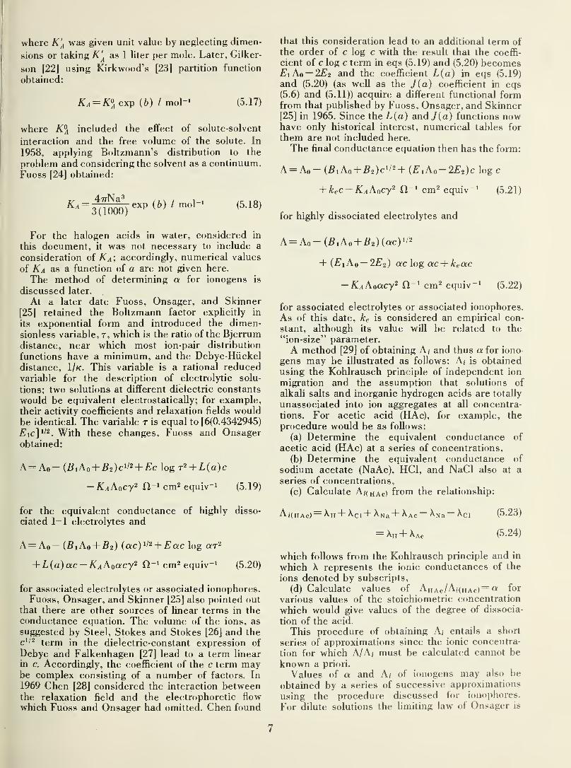
where K'A was given unit value by neglecting dimen-
sions or taking K'A
as 1 liter per mole. Later, Gilker-
son [22] using Kirkwood’s [231 partition function
obtained:
Ka = K°A exp ( b ) / mol -1(3.17)
where K°A included the effect of solute-solvent
interaction and the free volume of the solute. In
1958, applying Boltzmann’s distribution to the
problem and considering the solvent as a continuum,
Fuoss [24] obtained:
^=S) exp(6,/moH ,5 ' 18)
For the halogen acids in water, considered in
this document, it was not necessary to include a
consideration of Ka ;accordingly, numerical values
of Ka as a function of a are not given here.
The method of determining a for ionogens is
discussed later.
At a later date Fuoss, Onsager, and Skinner
[25] retained the Boltzmann factor explicitly in
its exponential form and introduced the dimen-
sionless variable, r, which is the ratio of the Bjerrum
distance, near which most ion-pair distribution
functions have a minimum, and the Debye-Hiickel
distance, 1 /k. This variable is a rational reducedvariable for the description of electrolytic solu-
tions; two solutions at different dielectric constants
would be equivalent electrostatically; for example,their activity coefficients and relaxation fields wouldbe identical. The variable r is equal to [6(0.4342945)
£V] 1/2. With these changes, Fuoss and Onsager
obtained:
A = A 0 — (B iA 0+ B 2 ) c1 '2 + Ec log T2 + L(a)c
— K^Aocy 2 fl_1 cm 2 equiv-1 (5.19)
for the equivalent conductance of highly disso-
ciated 1-1 electrolytes and
A= Ao~ (B 1A 0 + B 2 ) (ac) ll2 + Eac log ar 2
+ L(a) ac — K^Aoctcy 2 cm 2 equiv -1(5.20)
for associated electrolytes or associated ionophores.Fuoss, Onsager, and Skinner [25] also pointed out
that there are other sources of linear terms in the
conductance equation. The volume of the ions, as
suggested by Steel, Stokes and Stokes [26] and thec 1/2 term in the dielectric-constant expression of
Debye and Falkenhagen [27] lead to a term linear
in c. Accordingly, the coefficient of the c term maybe complex consisting of a number of factors. In
1969 Chen [28] considered the interaction betweenthe relaxation field and the electrophoretic flow
which Fuoss and Onsager had omitted. Chen found
that this consideration lead to an additional term of
the order of c log c with the result that the coeffi-
cient of c log c term in eqs (5.19) and (5.20) becomesF 1 A0 — 2E2 and the coefficient L(a
)
in eqs (5.19)
and (5.20) (as well as the J(a) coefficient in eqs(5.6) and (5.11)) acquire a different functional formfrom that published by Fuoss, Onsager, and Skinner
[25] in 1965. Since the L(a
)
and J(a) functions nowhave only historical interest, numerical tables for
them are not included here.
The final conductance equation then has the form:
A = A0 — (B\Ao + B 2 )cll2 -\- (E 1 Ao — 2E2 )c log c
+ kec— K^Aocy 2 O- 1 cm 2 equiv -1
(5.21)
for highly dissociated electrolytes and
A = A 0 — (B iA 0 + B 2 ) (ac)ll>2
+ (Ei A 0 — 2E2 ) ac log ac + keac
— K^Aoacy 2 li-1 cm 2 equiv -1
(5.22)
for associated electrolytes or associated ionophores.
As of this date, ke is considered an empirical con-
stant, although its value will be related to the
“ion-size” parameter.
A method [29] of obtaining A, and thus a for iono
gens may be illustrated as follows: A, is obtained
using the Kohlrausch principle of independent ion
migration and the assumption that solutions of
alkali salts and inorganic hydrogen acids are totally
unassociated into ion aggregates at all concentra-
tions. For acetic acid (HAc), for example, the
procedure would be as follows:
(a) Determine the equivalent conductance of
acetic acid (HAc) at a series of concentrations,
(b) Determine the equivalent conductance of
sodium acetate (NaAc), HC1, and NaCl also at a
series of concentrations,
(c) Calculate A,( HAc )from the relationship:
^i(HAc) = ^H+ ^Cl+ ^Na+ k Ac—
^Na ~~^-Cl (5.23)
= \H "f XAc (5.24)
which follows from the Kohlrausch principle and in
which X represents the ionic conductances of the
ions denoted by subscripts,
(d) Calculate values of AHAc /A;(HA c)= a for
various values of the stoichiometric concentration
which would give values of the degree of dissocia-
tion of the acid.
This procedure of obtaining A, entails a short
series of approximations since the ionic concentra-
tion for which A/A, must be calculated cannot be
known a priori.
Values of a and A,- of ionogens may also be
obtained by a series of successive approximations
using the procedure discussed for ionophores.
For dilute solutions the limiting law of Onsager is
7

used. Values of a at higher concentrations may be
obtained if the E and higher coefficients are known.
As a start these may be estimated and then iteration
is made until values of a, A,-, E , and the higher
terms are self consistent.
In many cases, complex ionic equilibria exist in
aqueous solutions and it is not possible to cate-
gorically cover all of these in a general fashion.
Instead each case will be considered individually
where necessary, as, for example, for HF considered
later in this document.A somewhat more detailed treatment of the
Debye-Hiickel-Onsager-Fuoss theory of electrolytic
conductance is given in appendix A.
The temperature range has been limited since waxor wax lined cells had to be used owing to the
corrosiveness of HF. This situation could beremedied, today, by using polyethylene containers
or other containers of plastic. The data in the
literature on HF have been reported on various
concentration scales, namely, mole percent, weightpercent, volume dilution, etc. These data were all
converted to the molarity basis using available
data on the density of aqueous solutions of HF.The density data were fitted to polynominals. the
constants for which are given in appendix B.
The dissociation of HF is controlled by the twoequilibria:
6. Determination of A 0
The method outlined by Fuoss and Accascina [15J
was followed, where possible, in determining A 0 .
As a start the Shedlovsky [30] function A„ given by
\'0= (A + B 2c 112
) I {l— BiC 11'2
) O -1 cm'2 equiv -1(6.1)
is calculated from observed values of A and the
theoretical constants B\ and B 2 . Values of Aq are
then plotted against c and a preliminary value of A 0
obtained by extrapolation to c = 0. This preliminary
value of Ao is then used to compute B\Ao + B 2
and E (or FhAo — 2E 2 ). Then values of A' given by
A' = A+ (B,Ao + B 2 )c'i*-Ec = Ao
+ kec H- 1 cm 2 equiv -1(6.2)
are plotted against c and the intercept at c = 0 gives
A 0 with the slope giving the empirical constant, k e .
In some cases the procedure must be iterated until
consistent values of A 0 (between (6.1) and (6.2)) are
obtained. The empirical constant corresponds to
the older functions J (a) or L(a) where E was equal
to FhAo — E2. Note here that E— E\A0 — 2E2.
7. Equivalent Conductances of HF,HC1, HBr, HI
Of the four halogen acids HF, HC1, HBr, HI all
are unassociated ionogens except HF which is not
only incompletely dissociated at finite concentra-tions, but exhibits association of the fluoride ion
and the undissociated molecule. These four acids
are considered in order. All data, where necessary,were converted to the Jones-Bradshaw [1] con-
ductance standard, the 12 C scale of atomic weights,and the absolute electrical units [2]. All data wereprogrammed for an IBM 7090 computer.
HF(a ) Equilibria. Data on the equivalent conductance
of HF are available only at 0, 16. 18. 20, and 25 °C.
HF H+ + F- (7.1)
and
HF2-^HF+F- (7.2)
with the first one more significant for dilute solu-
tions below 0.001 molar. The equilibrium constants
for these equilibria are given, respectively, by:
a H c H+ c F-y H
+ 7F_
mol /'
aHF chf7hf(7.3)
and
a HFa F
ahf:
cHFCF~Thf7f
chf7 7hf1mol /
-1(7.4)
where a, c, and y denote, respectively, the activity,
concentration, and activity coefficient of the species
denoted by the subscripts. If we let y and y2 be
the ratios, respectively, of the concentrations of
F _ and HFy to the stoichiometric concentration.
C, of HF, and assuming, as a start, that all activity
coefficients are unity, we have:
K%Qyir±isl^C(+)moU -,
1 y— 2y3 (7.5)
A = —- - - y 2y:i) ~— mot M (7.6)ya 73
The approximations given in eqs (7.5) and (7.6)
are obtained by setting 1 —7—273= 1.
Now the observed conductance of HF is given by:
A — 7A.0 +73A0 O -1 cm 2 equiv -1(7.7)
8

where Ao is the sum of the limiting equivalent
conductances of H + and F - and A0 is the sum of
the limiting equivalent conductances of HF .7 and H +.
Solving the approximate versions of eqs (7.5)
and (7.6) for y and y3 and substituting in (7.7)
gives:
A ( 1 -h c/A-) 1/2 = ( A„ VK/Vf
+ (\o y/~K I k) Vc n-J cm 2 equiv -1(7.8)
This equation may be converted to a linear form [35]
by multiplying by Vc, adding and subtracting
cAoV^/A to the right side, dividing by (l + c/A) 1/2,
squaring both sides, and simplifying; these steps
lead to:
cA2 = A§K + [2Xo/A 0— 1 + ( 1 — Xo/A 0 )
2/(l
+ k/c)]AlKc/kQ,~ 2 cm 4 equiv -2 (7.9)
At low concentrations the term ( 1 — Ao/Ao) 2/ ( 1 + k/c)
vanishes while at high concentrations it approachesasymptotically the limit (1
— A 0 /Ao) 2. Therefore,
this may be neglected when Xo/A 0 is sufficiently
close to unity to render (1 — X 0 /A 0 )2 negligible with
respect to (2X 0/A 0—
1). Accordingly, equation 7.9
reduces to:
cA2 = A 2K + c(2A 0 A 0 — \l)Klkil~2 cm 4 equiv -2
(7.10)
If we now introduce the ionic activity coefficient, y,
and the ionic mobility coefficient, m'
,
we have:
1-A/AoA%K
(2AqAq — A )K(7.11)
Values of y and m
'
are given, respectively, by:
log y = — A c VcA/Ao (7.12)
andm ’ = 1 — (Z?iAo + B>) A 7
1 VcA/Ao (7.13)
where A c is the Debye-Hiickel constant, given by:
2vN \ 1/2 e 3 / 1
1000/ 2.302585A 3/2\ T3l2 e 312
(7.14)
and B\ and B> are the Debye-Hiickel-Onsager con-
stants given, respectively, by eqs (5.4) and (5.5) andA c is the Debye-Hiickel constant in eqs (5.13), values
of which are listed from 0 to 100 °C in table 7.
A plot of values of the left side of eq (7.11) against
c (
1
— A/Ao) gives a straight line for molarities
^
/O 2 mol-1/ 2
between 0.004 and 1.0. The intercept whenc(l — A/A o)=0 gives AIK and the slope of the line
gives (2A 0A 0 — Al) K/k. Thus, since A 0 and A 0 are
known K and k can be evaluated (see below under(b).
(b) Values for Ao. Values reported for A 0 for HFare given in table 8 . The limiting equivalent con-
ductances of the ions at 25 °C as compiled byRobinson and Stokes [41] yield 405.0 for Ao for HF(their values were converted to absolute units here).
Erdey-Griiz, Majthenyi, and Kugler [42] using
Shedlovsky’s [43] A 0 values for HC1 and NaCl andtheir value for NaF obtained 405.04 on the old
Parker conductivity standard which becomes 405.09
on the Jones-Bradshaw standard. Using 126.39 for
A 0 for NaCl [41], 105.43 for Ao for NaF [42], and426.06 for Ao for HC1 (see later in this document)gives 405.10 for Ao for HF; this value was selected
here as the most reliable value for A 0 for HF at 25 °C.
Wooster [35] gave 255 and 404 for Ao at 0 and25 °C, respectively. Using the ratio 405.10/404,
Ao becomes 255.69 at 0 °C. From a linear plot of A 0
against 1 IT one obtains 354.29, 365.85, 377.26 for
Ao at 16, 18, and 20 °C, respectively. Wooster [35]
gave 437 and 275.4 for Ao at 25 and 0 °C, respectively.
On converting to the above basis and using a
(A 0 -l/r) plot, Ao values of 276.15, 383.08, 395.62,
407.99, and 438.19 are obtained, respectively, at
0 , 16, 18, 20, and 25 °C.
(c) Equivalent conductances of HF. The available
data on HF at 25 °C appear in papers by Deussen[37], Fredenhagen and Wellmann [34], Thomas andMaass [44], Ellis [45], and Erdey-Griiz, Majthenyi.
and Kugler [42]. Thomas and Maass reported their
results to only one decimal place and Erdey-Griiz
et al. only for very dilute solutions; the latter’s
data also appear low on a plot of eq (7.11). The data
of Deussen, Fredenhagen, and Wellmann, and of
Ellis agree within their experimental uncertainty
and were fitted to eq (7.11). Data at 16 and 20 °Cwere obtained only by Roth [36] while data at 18 °Cwere obtained both by Roth [36] and Hill andSirkar [31]. The data of Hill and Sirkar, however,were very much lower than those of Roth and wereinconsistent with the data obtained by other experi-
menters at other temperatures. For 0 °C, data were
obtained by Deussen and Hill and Sirkar; the
latter data showed erratic changes with concen-
tration and Deussen’s data at 0 °C were, therefore,
selected as the more reliable.
All of these data were fitted to eq (7.11). From a
plot of the values of the left side of eq (7.11) against
c(l— A/A 0 ), shown for 25 °C for example in
figure 1, the values given in table 9 were obtained
for K and A. The s x values, given in table 9. are
the standard deviation with which eq (7.11) was
fitted over the concentration range of 0.004 to
1.0 N for 0 °C; of 0.006 to 0.2 N for 16. 18. and
20 °C; and 0.004 to 1.0 N for 25 °C.
9

Eq 7.11 may be rearranged to give for A
A = AJK(y)2
(1-A/A„)C
+ (2AoA 0-A 2K)
^^ (1 — A/Ao)2
O- 1 cm 2 equiv -1
It was also found that
(m'/y) 2(1 — A/A 0 ) and (m'ly) 2
(1 — A/A 0
Values of ji, j[ , y 2 ,and j'
2follow:
t j i
• t
h J2•t
h Sx
°c n- 1 cm 2 equiv~ l
0 1.37 0.307 1.28 0.363 0.7
16 1.28 .230 1.26 .320 1.2
18 1.28 .230 1.26 .320 1.1
20 1.28 .230 1.26 .320 1.1
25 1.34 .268 1.29 .341 0.6
may be expressed, respectively, by:
(1 — A/A0 ) =ji+j[ log C (7.16)
and
(y)
2
(l-A/A0 )2=
72 +y; log C (7.17)
The sx values are the standard deviations with
which eq (7.18) was fitted over the concentration
range of 0.004 to 1.0 M for 0 and 25 °C and for
0.006 to 0.2 M for the other temperatures.
Values of the equivalent conductances of HFfor rounded concentrations are given in table 10.
Values at other concentrations, within the rangesgiven, may be calculated from eq (7.18).
Therefore, eq (7.15) may be written:
(2A 0X 0 A~K)A = ^lK{ji+j[ log C)C+
1/2
O'
2
+y; iogC) n- 1 cm 2 equiv-1 (7.18)
HC1
(a) Data at 25 °C. The equivalent conductances of
HC1 at 25 °C have been reported by Ruby and Kwai[46], Hlasko [47], Howell [48], Shedlovsky [43], Sax-
ton and Langer [49], Owen and Sweeton [50],
Klochko and Kurbanov [51], Stokes [52], and Murrand Shiner [53]. Of the earlier data given in the
Figure 1. Plots used to obtain values for K and k governing the dissociation o/HF.
A. No corrections made for activity coefficients or changes in ionic mobilities with concentration.B. Corrections made for activity coefficients.
C. Corrections made for activity coefficients and changes in ionic mobilities with concentration.
10

International Critical Tables only the data of
Hlasko and Howell are considered here; their data
were the most recent and were for higher concen-
trations where there is a sparsity of data.
It was necessary to divide the data into four con-
centration ranges to obtain reasonable least square
fits to the interpolation equation:
A = A0 — (B \Ao + #2 )
c
1 /2 + Ec log c + Ac
+ Be312 + Cc2 + Dc^l2 fl-1 cm2 equiv-1 (7.19)
(This equation is an extension of eq (5.21) which is
required for higher concentrations. When higher
concentrations are included the coefficient of the
c term differs from that obtained when lower con-
centrations are used). At low concentrations the
last two terms on the right were insignificant. Thefour concentration ranges were as follows:
Concentra-
tion rangeSx References
(molarity)
O-OMla-' cm 2eqiiiv~ x
0.05 [43], [49], [50], [52], [53]
0 .01-0.1 .14 [43], [46], [47], [49], [50],
0. 1-3.0 .10
[52]
[50], [51], [52]
3.0-11.6 .15 [47], [48], [50], [51]
The sx values are the standard deviation with whichthe following equations fit the experimental data:
0-0.01 M
A = 426.06-158.63 c J /2 + 185.76 clog c + 747.385 c
— 2095.71 c3/2 O- 1 cm2 equiv-1 (7.20)
0.01-0.1M
A = 426.06- 158.63c 1 / 2 + 173. llc-f 43.515c 3 / 2
— 345.46c 2 O -1 cm 2 equiv -1 (7.21)
0.1-3.0;4f
A = 426.06 - 158.63c 1 / 2 + 221 .501c - 252.771c 3 / 2
+ 115.606c 2 — 19. 5824c5/2 fl-1 cm 2 equiv-1 (7.22)
3.0-11.6M
A = 426.06 - 158.63c 1 / 2 + 143.554c - 116.628c3 /2
+ 35.2535c 2 — 3. 56231c5/2 fl-1 cm2 equiv -1
(7.23)
The coefficient of the c 1/2 term was obtained fromAo and the B\ and B2 coefficients of the Debye-Hiickel-Onsager theory. For the dilute range thecoefficient of the c log c term was obtained from A 0
and the E 1 and 2E 2 coefficients given in table 4(actually 185.767 which was rounded to 185.76).
For concentrations above 0.01 M it was found that
the c log c term was not needed. It was also foundthat the value of A 0 depended somewhat on the
source of the data used in the dilute range. Thedata of Shedlovsky, Saxton and Langer, Owen andSweeton, Stokes, and Murr and Shiner below 0.01
M were used to obtain A 0 , according to the pro-
cedure outlined by Fuoss and Accascina [15], with
the following results:
ExperimentersNumber
of
measure-ments
Ao
Shedlovsky 11
O -1 cm 2 equiv~ x
426.00
Q -1 cm 2 equiv~ x
0.07
Saxton andLanger 10 426.35 .08
Owen andSweeton 5 426.55 .07
Stokes 9 426.40 .04
Murr andShiner. 20 426.06 .02
Since s x for the A 0 value obtained from the dataof Murr and Shiner was the lowest their A 0 valuewas selected (evident on reference to eqs (7.20) to
(7.23)).
The equivalent conductances of HC1 at roundedconcentrations at 25 °C, and the experimental
range covered, calculated by eqs (7.20) to (7.23),
are given in table 11.
(b) Data at other temperatures. Values of the
equivalent conductance of HC1 at —20, —10, 0, 10,
20, 30, 40, and 50 °C, given here, are based on the
data of Haase, Sauermann, and Diicker [54], except
that at 50 °C the values in the dilute range (0 to
0.01 M) were derived from the results of Cook and
Stokes [55]. Values at 5, 15, 35, 45, 55, and 65 °C are
based on the results of Owen and Sweeton [50].
These results were consistent with those obtained
at 25 °C and discussed above.
The equivalent conductances of HC1 at rounded
concentrations for these temperatures and for the
experimental range covered are included in table 11.
The data in each case, except below 0 °C, were
fitted to the equation:
A = A 0 — Sc 1/2 + Ec log c + Ac + Bc'i,2Jr Cc'2
+ Z>c 5/2 0 -1 cm 2 equiv -1(7.24)
372-265 0 - 70 -311

where S= ZCAo + B> and B i, B% and E are the
theoretical Debye-Hiickel-Onsager-Fuoss coeffi-
cients. Below 0 °C the empirical equation
A= A + Be + Cc 2 + Dc 3 + Ec4 + Ec 5
+ Gc 6 El~ 1 cm 2 equiv -1(7.25)
was used. In this case A obviously doesn't represent
Ao as the infinitely dilute solution would be in the
solid or frozen state. Nevertheless eq (7.25) may beused for interpolation purposes.
Values of the coefficients of eqs (7.24) and (7.25)
and the concentration value over which they apply
are given in table 12. The 5 values given in column9 are the standard deviations of the fit.
HBr
(a) Data at 25 °C. Data on the equivalent con-
ductance of HBr at 25 °C are based on the measure-ments of Dawson and Crann [56]. Hlasko [47], andHaase, Sauermann, and Diicker [54]. Only the last
mentioned are recent data. As with HC1 the data
were divided into concentration ranges (in this
case three) to obtain reasonable least square fit
of the data with the equation:
A = A 0 — Sc ll2 + Ec log c+ Ac+ Be312 + Cc 2
+ Z)c5/2 0 _1 cm2 equiv -1(7.26)
The c In c term was not required above 0.01 M, andfor the dilute range the c 5/2 term was negligible.
The concentration ranges with the conductanceequations follow (the s values are the standarddeviations of the fit):
0.0000— 0.014/ (5 = 0.09; references [47, 56])
A = 427.74- 159.02c 1 /2 + 186.65c log c + 899.72c
- 4289.3c 3 /2 + 8912.1c 2 H -1 cm2 equiv" 1 (7.27)
0.01 — 0.104/ (5 = 0.09; references [47, 56])
A = 427.74- 159.02c 1 /2 + 210.8272c
— 209.547c3/2H _1 cm 2 equiv -1(7.28)
0.10— 3.04/ (5 = 0.08; references [47, 56])
A= 427.74- 159.02c 1 /2 + 192.8124c- 177.2474c 3 /2
+ 53.93903c2 -3.746204c5/2 O -1 cm 2 equiv -1(7.29)
3.0— 7.54/ (5 = 0.09; references [47, 54])
A = 427.74 - 159.02c 1 /2 + 130.5906c - 101 ,6916c3 /2
+ 29.49103c2 — 2.843402c5/2 fl-1 cm 2 equiv -1
(7.30)
As for HC1 the coefficient of the c 1/2 term wasobtained from Ao and the B i and Bo coefficients
of the Debye-Hiickel-Onsager theory.
The equivalent conductances of HBr at roundedconcentrations at 25 °C, calculated by eqs (7.27)
to (7.29) for the experimental range covered are
given in table 13.
(b) Data at other temperatures. Values of the
equivalent conductance of HBr at —20. — 10. 0. 10.
20, 30, 40, and 50 °C are based on the recent
measurements of Haase, Sauermann. and Diicker
[54]. The equivalent conductances of HBr at roundedconcentrations for these temperatures and for the
experimental range covered are given in table 14.
The data in each case, except below 0 °C, werefitted to the equation:
A = A 0~~ Sc 112 + Ac + Be 312 + Cc 2
+ Dc 5 /2 H -1 cm 2 equiv -1(7.31)
with a zero standard deviation. The coefficient S
again equals /?iA0 -t-/?2 . Below 0 °C the empirical
equation used for HC1. namely, eq (7.25) was again
used. Values of the coefficients of eqs (7.31) and
(7.25) (as applied to HBr) are given in table 15
together with the concentration range over whichthey apply. The coefficients are empirical and the
coefficient of the c term is low in terms of moderntheory.
HI
Only a few measurements have been made on the
electrolytic conductance of HI and. with the excep-
tion of those of Haase, Sauermann. and Diicker in
[54], these were made over 30 years ago. The Inter-
national Critical Tables (1929) cited two papers
for 18 °C, one by Loomis in 1897 [57] and the other
by Heydweiller in 1909 [58]. For 25 °C, the work of
Ostwald in 1903 [59], of Washburn and Strachan
in 1913 [60], and of Strachan and Chu in 1914 [61]
were cited. Ostwald's results were thrown in doubt
when Bray and Hunt [62] showed that his data for
HC1 were in error by about 3 percent and pre-
sumably his data on HBr were also questionable.
Washburn and Strachan's data were nullified by
analytical errors made in establishing the con-
centration of the solutions; Strachan and Chucorrected their data. Only three references to workon HI were found that had not been listed in ICT.
Two of these contained the same data. Hlasko and
Wazewski [63] and Hlasko [47]. The third one was
by Haase et al. mentioned above [54]. Solutions of
HI may also contain traces of iodine although
the experimenters made attempts to prevent HI
decomposition.
(a) Data at 25 °C. The data of Strachan and Chu,
Hlasko, and Haase et al. at 25 °C were combinedand fitted to a polynomial. The Ao for HI was
calculated from the ionic values listed by Robinson
and Stokes and converted to absolute units. Theequations are from 0.0000— 0.014/ and 0.01 — 7.04/
,
12
respectively, for the equivalent conductance as a
function of c at 25 °C
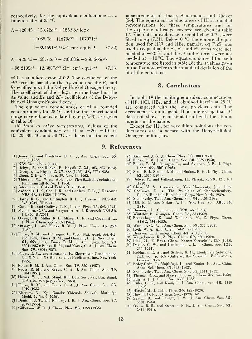
A = 426.45 - 158.72c 1 /2 + 185.96c log c
+ 1085.7c!— 1 1678c 3 /2 + 107071c 2
— 394591c5/2 fl-1 cm2 equiv -1
, (7.32)
A = 426.45 - 158.72c 1 /2 + 248.885c - 256.566
c
3 '2
+ 96.2195c 2 — 12.3887c 5 /2 fl-1 cm 2 equiv -1
(7.33)
with a standard error of 0.2. The coefficient of the
c 1 /2 term is based on the Ao value and the B\ andB 2 coefficients of the Debye-Hiickel-Onsager theory.
The coefficient of the c log c term is based on the
A 0 value and E\ and 2Ez coefficients of the Debye-Hiickel-Onsager-Fuoss theory.
The equivalent conductances of HI at roundedconcentrations for 25 °C and for the experimentalrange covered, as calculated by eq (7.33), are given
in table 16.
(b) Data at other temperatures. Values of the
equivalent conductance of HI at —20, —10, 0,
10, 20, 30, 40, and 50 °C are based on the recent
9. Re
[1] Jones, G., and Bradshaw, B. C., J. Am. Chem. Soc. 55,1780 (1933).
[2] NBS Circ. 459, 7 (1947).
[3] Debye, P., and Hiickel, E., Physik. Z. 24, 185, 305 (1923).
[4] Onsager, L„ Physik. Z. 27, 388 (1926); 28, 277 (1928).
[5] Chem. & Eng. News, p. 39, Nov. 11, 1963.
[6] Thiesen, M., Wiss. Abh. der Physikalisch-TechnischenReichsanstalt 4, No. 1, 1904.
[7] International Critical Tables 3, 25 (1928).
[8] Swindells, J. F., Coe, J. R., and Godfrey, T. B., J. ResearchNBS 48, 1 (1952) RP2279.
[9] Hardy, R. C., and Cottington, R. L., J. Research NBS 42,573 (1949) RP1994.
[10] Coe, J. R., and Godfrey, T. B., J. App. Phys. 15, 625 (1944).
[11] Malmberg, C. G., and Maryott, A. A., J. Research NBS 56,1 (1956) RP2641.
[12] Owen, B. B., Miller, R. C., Milner, C. E., and Cogan, H. L.,
J. Phys. Chem. 65, 2065 (1961).
[13] Onsager, L., and Fuoss, R. M., J. Phys. Chem. 36, 2689(1932).
[14] Fuoss, R. M., and Onsager, L., Proe. Nat. Acad. Sci. 41,283 (1955); Fuoss, R. M., and Onsager, L., J. Phys. Chem.61, 668 (1957); Fuoss, R. M., J. Am. Chem. Soc. 79,3301 (1957); Fuoss, R. M., and Kraus, C. A., J. Am. Chem.Soc. 79, 3304 (1957).
[15] Fuoss, R. M., and Accascina, F., Electrolytic Conductance,Ch. XIV and XV (Interscience Publishers, Inc., New York,1959).
[16] Fuoss, R. M., J. Am. Chem. Soc. 79, 3301 (1957).
[17] Fuoss, R. M., and Kraus, C. A., J. Am. Chem. Soc. 79,3304 (1957).
[18] Hamer, W. J., Nat. Stand. Ref. Data Ser., Nat. Bur. Stand.(U.S.), 24, 276 pages (Dec. 1968).
[19] Fuoss, R. M., and Kraus, C. A., J. Am. Chem. Soc. 55,1019 (1933).
[20] Bjerrum, N., Kgl. Danske Vidensk. Selskab. Math.-fys.
Medd. 7, No. 9 (1926).
[21] Denison, J. T., and Ramsey, J. B., J. Am. Chem. Soc. 77,2615 (1955).
[22] Gilkerson, W. R., J. Chem. Phys. 25, 1199 (1956).
measurements of Haase, Sauermann, and Diicker
[54], The equivalent conductances of HI at roundedconcentrations for these temperatures and for
the experimental range covered are given in table
17. The data in each case, except below 0 °C, werefitted to eq (7.31). Below 0 °C the empirical equa-tion used for HC1 and HBr, namely, eq (7.25) wasused except that the c4
,c5 , and c6 terms were not
needed at —20 °C and the c5 and c6 terms were not
needed at — 10 °C. The equations derived for eachtemperature are listed in table 18; the s values givenin the footnote refer to the standard deviation of the
fit of the equations.
8. Conclusions
In table 19 the limiting equivalent conductances
of HF, HC1, HBr, and HI obtained herein at 25 °C
are compared with the best previous data. Theagreement is quite good. It is interesting that A0
does not show a consistent trend with the atomic
number of the halide.
Except for HF, for very dilute solutions the con-
ductances are in accord with the Debye-Hiickel-
Onsager limiting law.
[23] Kirkwood, J. G., J. Chem. Phys. 18, 380 (1950).
[24] Fuoss, R. M., J. Am. Chem. Soc. 80, 5059 (1958).
[25] Fuoss, R. M., Onsager, L., and Skinner, J. F., J. Phys.
Chem. 69, 2581 (1965).
[26] Steel, B. J., Stokes, J. M., and Stokes, R. H., J. Phys. Chem.62, 1514 (1958).
[27] Debye, P., and Falkenhagen, H., Physik. Z. 29, 121, 401
(1928).
[28] Chen, M. S., Dissertation, Yale University, June 1969.
[29] Maclnnes, D. A., The Principles of Electrochemistry,
Ch. 18 (Reinhold Publishing Corp., New York, 1939).
[30] Shedlovsky, T., J. Am. Chem. Soc. 54, 1405 (1932).
[31] Hill, E. G., and Sirkar, A. P., Proc. Roy. Soc. A83, 140
(1910).
[32] Domange, L., Compt. rend. 198, 469 (1934).
[33] Winteler, F., Z. angew. Chem. 15, 33 (1902).
[34] Fredenhagen, K., and Wellmann, M., Z. Phys. Chem.A 162, 454 (1932).
[35] Wooster, C. B., J. Am. Chem. Soc. 59, 377 (1937).
[36] Roth, W. A., Ann. Chem. 542, 35 (1939).
[37] Deussen, E., Z. anorg. Chem. 44, 310 (1905).
[38] Wegscheider, R., Z. Phys. Chem. 69, 620 (1909).
[39] Pick, H., Z. Phys. Chem. Nernst-Festschrift, 360 (1912).
[40] Davies, C. W., and Hudleston, L. J., J. Chem. Soc. 125,260 (1924).
[41] Robinson, R. A., and Stokes, R. H., Electrolyte Solutions,
2nd. ed., p. 465 (Butterworths Scientific Publications,
London, 1959).
[42] Erdey-Gruz, T., Majthenyi, L., and Kugler, E., Acta Chim.
Acad. Sci. Hung. 37,393 (1963).
[43] Shedlovsky, T., J. Am. Chem. Soc. 54, 1411 (1932).
[44] Thomas, D. K., and Maass, O., Can. J. Chem. 36, 744 (1958).
[45] Ellis, A. J., J. Chem. Soc. 4300 (1963).
[46] Ruby, C. E., and Kwai, J., J. Am. Chem. Soc. 48, 1119
(1926).
[47] Hlasko, M., J. Chim. Phys. 26, 125 (1929).
[48] Howell, O. R., J. Chem. Soc. (1929) 162.
[49] Saxton, B., and Langer, T. W., J. Am. Chem. Soc. 55,
3638 (1933).
[50] Owen, B. B., and Sweeton, F. H.. J. Am. Chem. Soc. 63,
2811 (1941).
13

[51] Kloehko, M. A., and Kurbanov, M. Sh., Akad. Nauk SSSR,Izvest. sek. Fiz-Khim. analiza 24 , 237 (1954).
[52] Stokes, R. H., J. Phys. Chem. 65 , 1242 (1961).
[53] Murr, B. L., Jr., and Shiner, V. J., Jr., J. Am. Chem. Soc.
84 , 4672 (1962).
[54] Haase, R., Sauermann, P. F., and Diicker, K. H., Z. Phys.Chem. Neue Folge 47 , 224 (1965).
[55] Cook, B. M.. and Stokes, R. H., J. Phys. Chem. 67, 511(1963).
[56] Dawson, H. M., and Crann, T. W., J. Chem. Soc. 109 , 1262
(1916).
[57] Loomis, E. H., Ann. Physik. und Chemie 296 [3], 60, 547(1897).
[58] Heydweiller, A., Ann. Physik. 30 , 873 (1909).
[59] Ostwald, W., Lehrbach der allgemeinen Chemie, (Engel-
mann, Leipzig, 1903).
[60] Washburn, E. W., and Straehan. E. K., J. Am. Chem.Soc. 35 , 690 (1913).
[61] Straehan, E. K., and Chu, V. G., J. Am. Chem. Soc. 36 ,
810 (1914).
[62] Bray, W. C., and Hunt, F. L., J. Am. Chem. Soc. 33, 781
(19H).
[63] Hlasko, M., and Wazewski. D., Bull, intern, acad. Polonaise,
No. 4-5A, 181 (1928).
[64] Ref. 29, page 342.
[65] Harned, H. S., and Owen, B. B., The Physical Chemistry of
Electrolytic Solutions, 3rd ed., p. 231 (Reinhold Pub-lishing Corp., New York, 1958).
[66] Ref. 41, page 465.
10. Appendix A. The Debye-Hiickel-lytic Conductance
According to the Debye-Hiickel theory of electro-
lytic solutions, in the electrostatic effect betweenions, the discrete charge distribution is replaced bya continuous charge distribution, or charge density,
p(r), or “ion atmosphere” which is a continuousfunction of r, the distance from a reference ion. The“ion atmosphere” extends from r—a to
r=0(V1/3)~
where V is the volume of the system, and acts elec-
trostatically somewhat like a sphere of charge — e at
a distance k _i from the reference ion of charge+ e. The distance k -1
is considered the thickness
of the “ion atmosphere”.
Thermal or Brownian motion of the ions will
tend to disturb this distribution but not entirely so,
and Debye and Hiickel used the Boltzmann prin-
ciple to express the ionic distribution as a function
of the ratio of the electrical and thermal energies.
The localized concentration of a given species of
ions is equal to the average or bulk concentration
of that species multiplied by the exponential func-
tion exp (— U/kT ) where U gives the potential
energy at the point under consideration. If we havea solution containing Ni ions of species i(i — 1 , 2
for simple ions and 1,2 . . .5 for electrolyte mix-
tures) in a volume V, the localized (average) con-
centration riji of ionic species i in vicinity of ionic
species j is given by
riji= niexp (— Uji/kT ) (A.l)
where ni= Ni/V. The potential energy t/p of ani-ion with charge z,e near a 7-ion is given by z/eT]’
where e is the elementary charge, z; the valence of
an i-ion, and TT is the electrostatic potential at the
location of the i-ion, stated in terms of a spherical
coordinate system with the origin at the location of
the 7-ion (or reference ion). The thermal energy is
given by kT. Since f/= z,e xBj) eq (A.l) may be written:
(A.2)
Onsager-Fuoss Theory of Electro-
Since each i-ion has a charge z,e the net chargedensity of i-ion in the vicinity of a 7-ion, pj, is
given by
pj = ^ n/z/e exp (— neW^/kT) (A.3)
i
Debye and Hiickel also used Poisson’s equation
to relate pj and Tj, namely,
V*F«==i%j (A.4)
where e is the dielectric constant of the medium in
which the ions exist. This relation states that at
any point in a medium located by three spacecoordinates (x, y, z; r, d, $) the divergence of the
gradient of the potential is proportional to the
charge density at this point. Eliminating pj betweeneqs (A.3) and (A.4) gives
— 477V 2 xE?= V /i,-z/e exp (— z,e 'B9/&7’) (A.5)
J £ J
This relation implies a contradiction of the super-
position principle of electrostatics, namely, that
the potential due to an assembly of charges is simplythe sum of the potentials due to each of the chargesacting alone. The left side of eq (A.5) is a linear
function of 'E whereas the right side is not; it is
exponential. Debye and Hiickel resolved this
dilemma by restricting the application to dilute
solutions where the ionic potential energy is small
compared with the thermal energy (see eq (A. 7)
below).
For unperturbed electrolytic solutions the
“ionic atmosphere” is assumed to be spherical.
Therefore, it is most convenient to express V 2 xE;
in spherical coordinates, thus,
f1 dr\ dr j—^ mzie exp (
— Zietyj/kT)
(A.6 )riji = rii exp (— Zie^j/kT)
14
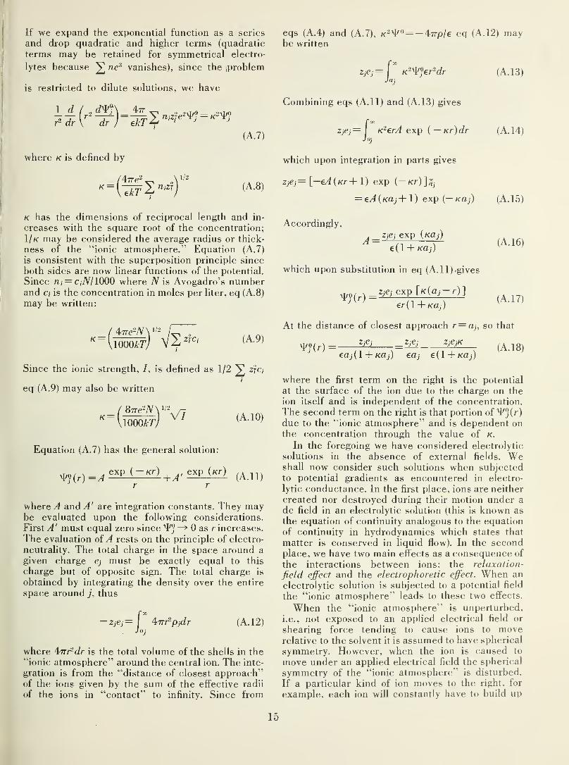
If we expand the exponential function as a series
and drop quadratic and higher terms (quadratic
terms may be retained for symmetrical electro-
lytes because ne2 vanishes), since the iproblem
is restricted to dilute solutions, we have
ld_r2 dr
mzfe2^(A.7)
where k is defined by
K = (A.8)
eqs (A.4) and (A.7), k 2^° = — 47rp/e eq (A. 12) maybe written
ziej=
I K2y¥^er2dr (A. 13)Jdj
Combining eqs (A. 11) and (A. 13) gives
Zjej= I K2erA exp (-Kr)dr (A. 14)Jaj
which upon integration in parts gives
zjej= [—eA ( kt + 1 ) exp (—#cr)]g)
= eA (Ka,j+ 1) exp (— Ka,j) (A.15)
k has the dimensions of reciprocal length and in-
creases with the square root of the concentration;
1Ik may be considered the average radius or thick-
ness of the “ionic atmosphere.” Equation (A.7)
is consistent with the superposition principle since
both sides are now linear functions of the potential.
Since rn= CiN/1000 where A is Avogadro’s numberand c, is the concentration in moles per liter, eq (A.8)
may be written:
Accordingly,
. _ zjej exp (Kdj)
e(l + Kdj)
which upon substitution in eq (A. 11) /gives
it/q/ \ __W exp [ic(aj-r)]
er(l + Kdj)
(A. 16)
(A.17)
K= 4<7re2N \ 1/2
/v1000AT/ VS ZrC!' (A.9)
Since the ionic strength, /, is defined as 1/2 ^ zjCj
i
eq (A.9) may also be written
k = (A. 10)
Equation (A.7) has the general solution:
/M (r)=J4exP (
- Kr)+ /l'
eXpUr>(A. 11)
Jr r
where A and A' are integration constants. They maybe evaluated upon the following considerations.
First A' must equal zero since —» 0 as r increases.
The evaluation of A rests on the principle of electro-
neutrality. The total charge in the space around a
given charge ej must be exactly equal to this
charge but of opposite sign. The total charge is
obtained by integrating the density over the entire
space around thus
~m= (A. 12)
where 47ri^dr is the total volume of the shells in the
“ionic atmosphere” around the central ion. The inte-
gration is from the “distance of closest approach”of the ions given by the sum of the effective radii
of the ions in “contact” to infinity. Since from
At the distance of closest approach r~dj, so that
^)'(r)z
)e
i = ZjCj ziejK
edj ( 1 + Kdj ) edj e ( 1 + Kaj
)
(A.18)
where the first term on the right is the potential
at the surface of the ion due to the charge on the
ion itself and is independent of the concentration.
The second term on the right is that portion of 4^(r)due to the “ionic atmosphere” and is dependent onthe concentration through the value of k.
In the foregoing we have considered electrolytic
solutions in the absence of external fields. Weshall now consider such solutions when subjectedto potential gradients as encountered in electro-
lytic conductance. In the first place, ions are neither
created nor destroyed during their motion under a
dc field in an electrolytic solution (this is known as
the equation of continuity analogous to the equation
of continuity in hydrodynamics which states that
matter is conserved in liquid flow). In the secondplace, we have two main effects as a consequence of
the interactions between ions: the reldxdtion-
field effect and the electrophoretic effect. When an
electrolytic solution is subjected to a potential field
the “ionic atmosphere” leads to these two effects.
When the “ionic atmosphere” is unperturbed,
i.e., not exposed to an applied electrical field or
shearing force tending to cause ions to moverelative to the solvent it is assumed to have spherical
symmetry. However, when the ion is caused to
move under an applied electrical field the spherical
symmetry of the “ionic atmosphere” is disturbed.
If a particular kind of ion moves to the right, for
example, each ion will constantly have to build up
15

its ionic atmosphere to the right while the charge
density to the left gradually decays. The rate at
which the atmosphere to the right forms and the
one on the left decays is expressed in terms of a
quantity known as the time of relaxation of the
“ionic atmosphere.” The decay occurs exponen-tially and the return is asymptotic to the original
random distribution. The time required for the
“ionic atmosphere” to fall essentially to zero is
given by 4qd where 6 is the time of relaxation and
q is defined by
z+z- / A.+ + X- \
^ z+ + \z+X+ + Z-\~)(A.19)
with z+, z- ,k+, and having the same significance
as given previously.
The asymmetry of the ion atmosphere owing to
the effect of the time of relaxation leads to an excess
charge of opposite sign behind the moving ion.
This excess charge of opposite sign causes a retarda-
tion of the moving ion. Onsager by using the
Debye-Hiickel approach, taking care of the
Brownian movement of the ions, and dropping
higher terms in the equation of continuity obtained:
AT,=- grad ^(„m = —2-= k* (A.20 )' 3ekTl + Vq
for the relaxation effect for a dilute electrolyte
solution dissociating into' two kinds of ions. Here
q is defined by eq (A.19), X is the electrical field
intensity acting in the x direction and X\ is the
relaxation field acting in the same direction but
in the opposite sense, as a result of the perturbation
of the “ionic atmosphere.” The resultant field is
then:
X+Xr=X+—
—
—^kX (A.21 )
3ekT 1 + \fq
The total electrical force acting on the ion is then
,(* +*0^4+^^) (A.22)
which leads to a movement of the ion with a velocity,
vf of:
v) = ej(X + Xi)uf = ejX ^1 4
(A.23)
where uf is the “absolute” mobility of the ion.
Since the product eie2 is negative, the relaxation
field opposes the external field.
The other factor, the electrophoretic effect,
arises from the tendency of the “ionic atmosphere”shell to move with its associated solvent moleculesunder an applied electrical field in a direction oppo-
e\e2
3ekT 1 4-V <7
K I U
site to the motion of the ion. The forces, kj, acting
on the ions must be balanced by other forces acting
on the solvent molecules, ks , hence:
X njkj=— n sks (A.24)
where bulk concentrations are denoted by nj
and n s. At a distance r from the central ion andwithin a volume element, dV, the localized con-
centration for the ion will differ from the bulk
concentration and the directed ion force neara 7-ion will be ^ njjkjdV which differs from the gross
volume average force mk\dV because of thei
7-ion concentrations within its vicinity (see later).
For the solvent molecules, the force remains un-
changed and is given by n sk„dV for the volume ele-
ment dV. The net force acting on the volumeelement near a /-ion is, therefore,
(\ njiki + nsks\ dV=^ ( n,-,-— m)kidV (A.25)' t ' i
A spherical shell of radius r and thickness dr is,
therefore, subject to the resultant force, d
,
given by:
dSP = ^ ( nji — rii ) ki (\nr2dr) (A.26)
i
Neglecting the asymmetry of the “ion atmosphere”,Fuoss used the distribution function:
nji =ni [l-eiV?/kT+$ (e^f/kT) 2] (A.27)
to express (% — ni
)
as a function of r and the
Debye-Hiickel expression (eq (A. 17)) for the poten-
tial T/j° (r). Thus, the resultant force on the shell is
given by:
dfX = 47rr2 ^ [— n& ,ej ( 1 4- Ka,
)
i
exp (— Kr)/ekTr exp
(
ko,) + n,e,ej(l 4- Ka,) 2
exp (— 2/cr)/2(e/f7V) 2 exp (2/<«, )] X Zjedr (A.28)
where ki is replaced by the electrical force, Ae,.
Debye and Hiickel originally considered that this
force imparted a velocity to the reference ion whichthey assumed followed Stokes law (eq (3.4)) for a
rigid sphere having a radius = b (hydrodynamicradius). Later Onsager considered that the force
(eq (A.28)) imparted a velocity to the reference ion
and its atmosphere which he assumed followed
Stokes volume equation:
dvj' — d^ffjriqr (A.29)
where p is the viscosity of the medium and the
average radius = r, thus eliminating the hydrody-
namic parameter b (see also Fuoss and Accascina
[15], p. 164). The total velocity, At;/, produced by
16

all the ions in the atmosphere on the 7-ion is thengiven by the integral of the combination of eqs (A.28)
and (A.29) from the “distance of closest approach”of the ions, a, to infinity, or:
2ziz2ql{l + Vq) we have:
/ e2W,
ezj \
At)j'=(|
r)j
j[-A, exp (— nr
)
+ Ao exp (— 2Kr)/r]dr (A.30)
Inserting values of A\ and A 2 from (A.28) gives:
Av"=— 2Xej meySiqekTK ( 1 + Ka)
+ Xej( 1 + Ka) 1Ei(2Kd)
^ rc,ef/3i7(e/T) 2 exp (2Ka) (A.31)
where Ei (2Ka) is the exponential integral e~2K,'dr.
For symmetrical electrolytes ei = e2 and the secondterm of equation (A.31) vanishes. Thus,
Av"=— 2Xejei^ nie']/3riekT(l + ka) (A.32)
Multiplication of the numerator and denominatorof (A.32) by k and substitution in the denominatorof the value for k2 given by (A. 8) give for Av"
Av"= — XejKl6Trr)(l + Ka) (A.33)
which is the original result presented by Onsager.If a = 0 (ions are point charges)(A.33) becomes:
Av"=— XejKl6irr} (A.34)
the limiting value derived by Onsager.Combining (A.23) for the relaxation effect and
(A.34) for the electrophoretic effect gives:
vj= vj + Av"
=Aur+£irrkv=g
u? - Kl67rn)
,A -35)
for the velocity of the ion. Since ejXu* = Vj 0 this
equation may be written, for an electrolyte contain-
ing two kinds of ions:
/ 4>7re2N Y 1
'2
r-——
—
V1000A-77Vz
'Cl + ^C2 - (A.37)
Onsager replaced Ci and c2 by equivalent concen-trations (c is then the same for both types of ions),
here denoted by c; hence:
(e2WVj= V
j°-{tekfVj°
/ 477e 2 /V\ 1/2
UOOOAT/V(| Zi
I+ |z2 |)c. (A.38)
For uni-univalent electrolytes zi = z2 =l andr=2 - V2
,
/e2 (2- V2)Vj= Vj°~{- '
6ekTVjo +
'
8 ire2N Y 12 r-
:ioooat/Vc (A.39)
Now for a potential gradient of 1 V/cm,
V= 1/299.7923 esu
and letting Vj/299.7925 = Uj, the mobility, we have:
Uj= Ujo-
e2 (2 — V2)
6ekTUjo-
ezi
6(299.7925)77r?)
(87
\1000A77V^‘ (A.40)
Now, since UjF=kj, where kj is the equivalent
conductance of the 7-ion, eq (A.40) may be written:
/e2(2-V2
)
k> kj °' 6eAT
kj°
ezjF \
6 (299. 7925) 77V/ 87re2NYl2 n\1000AT/
VC> (A.41)
Since e = 299. 7925 F/N eq (A.41) may also be
written:
|
ziz2| q
3ekT i +KVj 0
ezj
67717K (A.36)
where the valence of the ions, z, is now introduced.
Upon introduction of k as defined by (A.9) and sub-stitution of z2Ci "b z|c2 for ^ zfc,- and W for
kj— k/e-(2 — V2) zjP \
\ 6eAT j " 6Nnri)
/8ne2NYl 2 r(lOOOAT/
^ (A.42)
Now the equivalent conductance, A, of an electro-
lytic solution is the sum of the equivalent con-
17

ductances of the constituent ions, thus:
A = Aoe 2 (2 — V2) | z iz 2
1. (zi+ z 2 )F'- \
6ekT ° 6Nttti )
/ 87reW \ 1/2
V 1000AT /
Vc H- 1 cm 2 equiv 1
which may be written in the form:
A = Ao~ (R1A0 + R2 ) Vc H -1 cm 2 equiv
where B 1 and #2 denote, respectively,
6ekT \ 1000kT )
and
5 ,
(z,+z 2 )F2/ 87reW V /2
()N7TTj \ 1000AT /
1
(A.43)
(A.44)
(A.45)
(A.46)
(See also eqs (5.4) and (5.5)). Equation (A.44) is the
limiting law of Onsager.The Onsager equation, as stated above, gives the
tangent to the conductance curve at zero con-
centration; it is based on point charges as the modelfor the ions. In 1932, Onsager and Fuoss recalcu-
lated the electrophoresis term, using chargedrigid spheres to represent the ions. For symmetricalelectrolytes the electrophoretic term BoC 112 wasreplaced by BoC 112
1 (1 + Ka)
.
Later in a series of
papers Fuoss and Onsager gave a more compre-
hensive treatment in v,nich they retained the
higher terms in the Boltzmann factor and the
equation of continuity and gave a list of numericalvalues for certain transcendental functions related
to the exponential integral functions. In their com-prehensive treatment they considered ions as
charged spheres rather than point charges, included
the osmotic-pressure and viscosity effects, andused Oseen’s equation for the volume force rather
than Stokes’ equation for directional force to obtain
the ionic velocity in the field direction. A rather
complicated expression for the electrophoretic
term resulted; it was shown however, by Fuoss andHsia that the function could be closely approxi-
mated up to about 0.1 M for 1-1 electrolytes in waterby the 1932 result of Onsager and Fuoss. In 1969
Chen found that Fuoss and Onsager had omitted
an interaction between the relaxation field and the
electrophoretic flow, which leads to an additional
term of the order of c log c with the result that the
coefficient of the c log c term in eqs (5.6) and (5.11)
of the main text becomes FiA 0 — 22? 2 and the L(a
)
function (see eqs (5.19) and (5.20)) acquires a dif
ferent functional form 1 from that published in 1965The replacement of E 2 by 2Eo has little effect onthe values of the limiting conductance obtained
by extrapolation because E 2 is small comparedto E 1 Ao. The final equations resulting from the
theory are eqs (5.21) and (5.22) in the main text.
A. Bibliography for Appendix A[1] Fuoss. R. M., and Accascina. F., Electrolytic Conductance
(Interscience Publishers, Inc., New York, 1959).
[2] Harned. H. S., and Owen, B. B.. The Physical Chemistry of
Electrolytic Solutions, 3rd ed., Ch. 4 (Reinhold Publishing
Corp., New York, 1958).
[3] Robinson, R. A., and Stokes, R. H., Electrolyte Solutions,
2nd ed., Ch. 7 (Butterworth Scientific Publications,
London, 1959).
[4] Fuoss, R. M., and Onsager, L., J. Phys. Chem. 66, 1722
(1962); 67, 621, 628 (1963); 68, 1 (1964).
[5] Fuoss, R. M., Onsager, L., and Skinner, J. F., J. Phys. Chem.69, 25_81 (1965).
[6] Fuoss. R. M., and Onsager, L., Proc. Nat. Acad. Sci., U.S.
[7] Fuoss, R. M., and Onsager, L., J. Phys. Chem. 61, 668
(1957).
[8] Fuoss, R. M., J. Am. Chem. Soc. 79, 3301 (1957).
[9] Fuoss, R. M.. and Onsager, L., Proc. Nat. Acad. Sci., U.S.
47, 818 (1961).
[10] Onsager, L., and Fuoss, R. M.. J. Phys. Chem. 36, 2689
(1932).
[11] Onsager, L„ Physik. Z. 27, 388 (1926); 28, 277 (1927).
[12] Debye, P„ and Hiickel. E.. Physik. Z. 24, 185. 305 (1923).
[13] Fuoss, R. M., and Hsia, K. L., Proc. Nat. Acad. Sci., U.S.
57, 1550; 58, 1818 (1967).
[14] Chen, M. S., Dissertation, Yale University, June 1969.
41, 274, 1010 (1955).
11. Appendix B. Densities of aqueous solutions of HF
d= A + Bx + Cx2 + Dx3 + Ex4 + Fx5
x = weight percent
t Range A Bx\0 :i CX 105 Dx 107 £X108 FX10 10s
a Xl04
°c0
wt %0-30 0.99987 3.92 *1.14 12.5
0 0-55 .99987 4.705 -4.451 5.675 29.20
15
0-1000-36
.99987
.99913
4.6518
3.53
-3.5739*5.15
-1.8571 2.3603 -2.3029 73.1
5.015 0-54 .99913 3.507 *6.143 5.0
18 0-30 .99862 3.97 -1.56 5.0
20 0-30 .99823 4.06 - 1.85 3.9
25 0-36 .99707 4.39 — 1.71 3.0
25 0-66 .99707 4.8587 -7.2689 *1.8184 -1.6497 9.8
a — standard deviation of 1 it to equation 18 °C — E. G. Hill and A. P. Sirkar 31]* - X 106 20 °C - F. Winteler [33]
0 °C — E. G. Hill and A. P. Sirkar [31] 25 °C — K. Fredenhagen and M. Wellmann [34]
15 °C — L. Domange [32]
18

12. Appendix C. Use of the Systeme International d’Unites
In 1964 the National Bureau of Standards adoptedthe International System of Units (abbreviated SI
for Systeme International). This International Sys-
tem of Units was defined and given official status
in a resolution of the 11th General Conferenceon Weights and Measures which met in Paris
in October 1960. The SI is based on the meter(m) as the unit of length; the kilogram (kg) for
mass; the second (s) for time; the ampere (A)
for electric current; the Kelvin (K) for temperature;and the candela (cd) for luminous intensity. Ofthese units, those for mass, length, time, and tem-
perature are independent; that is, a definition of
one does not depend on definitions of others. How-ever, the ampere and the candela involve other units
in their definition. For example, the ampere involves
the units of length, mass, and time and is defined
as the magnitude of electricity that, when flowing
through each of two long parallel wires separated
by one meter in free space, results in a force be-
tween two wires (owing to their magnetic fields) of
2X10 -7 newton (N) (kg m s-2
) for each meter of
length. The candela needs not concern us here.
As has been customary heretofore in dealing
with the electrolytic conductance of solutions, the
cgs (centimeter-gram-second) system of units wasused in this paper. In converting to the SI systemthe following changes are required:
General— The unit of length is changed from the
centimeter to the meter, the unit of mass from thegram to the kilogram, the unit of force from the
dyne to the newton, and the unit of energy fromthe erg to the joule (J). Concentrations are then
expressed in kilomoles or kiloequivalent per cubicmeter. The ionic velocity (t>) is given in m s
_1rather
than cm s_1 and the “electrical mobility” of an ion
see page 3) would be the velocity attained by anon under a unit of potential gradient of 1 V permeter rather than 1 V per centimeter. Accordingly,equivalent conductances would retain the valuescommonly used, but with the unit being m 20_1
kequiv -1. The elementary charge is also given in
coulombs rather than in electrostatic units and ion
sizes are expressed in fractions of the meter rather
than in angstroms.Theoretical constants in the expressions for
equivalent conductances and activity coefficients— In
converting to SI, the following changes are required:
(1) In equations 4.8, 4.9, 4.10, 5.1, 5.2, 5.15,
5.18, 7.14, A.9, A.10, A.37, A.38, A.39, A.40, A.41,
A.42, A.43, A.45, and A.46 1000 (moles per liter) is
replaced by 1 m 3.
(2) Since the unit of charge is not defined throughCoulomb’s law on SI, e is replaced by e/ (47reo) 1/2 in
all equations where e appears. The constant, eo is
known as the permittivity of free space and has the
value 8.8541 7(3)>fcO- 12C 2J-
1m- 1.
(3) The constants in the various equations havethe following values:
k = 1.38054(18) X10~23J deg-'
N
=
6.02252(28) XlO26 kmoU 1
e= 1.60210(2) X10“ 19CF = 9.64870(16) X10 17C kequiv- 1
and the unit of viscosity is 10 _1 N s m -2. Here as
in the text, the numbers in parentheses represent
established limits of error.
13. Tables
Table 1 . Specific conductances of standard aqueous solutions o/KCl
Demal* Grams KC1 per 1000
g solution in vacuum
Specific conductances, f1 1 cm at
0 °C 18 °C 25 °C
1.0 71.1352 0.065144 0.097790 0.111287
0.1 7.41913 .0071344 .0111612 .0128496
.01 0.745263 .00077326 .00121992 .00140807
*Based on the international atomic weights of 1933.
19

Table 2. Physical properties of water
Temperature Density " Viscosity 6 Dielectric
constant c
t d 0 e
°C g/ml cP
0 0.99987 1.787 d 87.74 (87.90)
5 .99999 1.517 85.76 (85.90)
10 .99973 1.306 83.83 (83.95)
15 .99913 1.138 81.95 (82.04)
18 .99862 1.053 80.84 (80.93)
20 .99823 1.002 80.10 (80.18)
25 .99707 0.8903 78.30 (78.36)
30 .99567 .7974 76.55 (76.58)
35 .99406 .7194 74.83 (74.85)
38 .99299 .6783 73.82 (73.83)
40 .99224 .6531 73.15 (73.15)
45 .99025 .5963 71.51 (71.50)
50 .98807 .5471 69.91 (69.88)
55 .98573 .5044 68.34 (68.30)
60 .98324 .4669 66.81 (66.76)
65 .98059 .4338 65.32 (65.25)
70 .97781 .4044 63.86 (63.78)
75 .97489 .3782 62.43 (62.34)
80 .97183 .3547 61.03 (60.93)
85 .96865 .3340 59.66 (59.55)
90 .96534 .3149 58.32 (58.20)
95 .96192 .2976 57.01 (56.88)
100 .95838 .2822 55.72 (55.58)
a M. Thiesen [6]; International Critical Tables [7].
bJ. F. Swindells, J. R. Coe, and T. B. Godfrey [8],
R. C. Hardy and R. L. Cottington [9]; and J. R. Coe and
T. B. Godfrey [10].
c C. G. Malmberg and A. A. Maryott [11].
d Values in parentheses are those found by B. B. Owen,
R. C. Miller, C. E. Milner, and H. L. Cogan [12]; values
above 70 °C were calculated from their equation express-
ing the values obtained at lower temperatures as a
function of temperature.
TABLE 3. Values of the Debye-Hiickel-Onsager constants
Bi and B 2 for equivalent conductances for l—l aqueous
solutions from 0 to 100 °C
t B x B~,
°C l112 equiv~ 112 H- 1 cm2
1112 equiv~ 3,2
0 « 0.2211 (1) a 29.817 (6)
5 .2227(1) 35.206(8)
10 .2244(1) 40.995(9)
15 .2261(1) 47.169(10)
18 .2272(1) 51.060(11)
20 .2280(1) 53.722(11)
25 .2300(1) 60.639(13)
30 .2321(1) 67.906(14)
35 .2343(1) 75.508(16)
38 .2357(1) 80.240(17)
40 .2366(1) 83.449(18)
45 .2391(1) 91.711(19)
50 .2416(1) 100.31 (2)
55 .2443(1) 109.20 (2)
60 .2471(1) 118.42 (3)
65 .2499(1) 127.94 (3)
70 .2529(1) 137.79 (3)
75 .2560(1) 147.94 (3)
80 .2593(1) 158.41 (3)
85 .2627(1) 169.95 (4)
90 .2662(1) 179.99 (4)
95 .2698(1) 191.32 (4)
100 .2737(1) 202.71 (4)
" The numbers in the parentheses gives the ± un-
certainty in the last decimal arising from the uncertainties
in the physical constants.
20

TABLE 4. Values of the Fuoss-Onsager Ei and E 2 con-
stants for equivalent conductances for 1—1 aqueous
solutions from 0 to 100 °C
t Ei Ez a
°c 1 equiv~ xfl
_1cm 2/ equiv~ 2
0 b 0.4922(3) b 9.72(1)
5 .4992(3) 11.56(1)
10 .5066(3) 13.56(1)
15 .5146(4) 15.72(1)
18 .5196(4) 17.10(1)
20 .5233(4) 18.06(1)
25 .5325(4) 20.56(1)
30 .5422(4) 23.23(1)
35 .5526(4) 26.08(1)
38 .5591(4) 27.88(1)
40 .5637(4) 29.11(1)
45 .5754(4) 32.32(1)
50 .5876(4) 35.73(2)
55 .6008(4) 39.33(2)
60 .6145(4) 43.13(2)
65 .6287(4) 47.14(3)
70 .6439(4) 51.37(3)
75 .6599(5) 55.83(3)
80 .6768(5) 60.55(3)
85 .6945(5) 65.42(4)
90 .7132(5) 70.63(4)
95 .7328(5) 76.10(4)
100 .7538(5) 81.77(5)
3 Note that 2E2 is involved in the final conductance
equations (eqs (5.21) and (5.22)).
b The numbers in the parentheses give the ± uncer-
tainty in the last decimal arising from the uncertainties
in the physical constants.
Table 5. Differences in the values of Bi and B 2 from
those given in table 3 if the dielectric constants of
water determined by Owen et al. are used instead of
those of Malmberg and Maryott*
t AB, ABi
°C D 12 equiv~ ij
2
fl_1 cm 2
Iff2 equiv
~3/2
0 -0.0006 -0.027
5 - .0005 -.029
10 - .0005 -.029
15 - .0004 -.026
18 - .0004 -.028
20 - .0003 -.027
25 - .0003 -.024
30 - .0001 -.014
35 - .0001 -.010
38 0.0000 -.006
40 .0000 0.000
45 .0001 .006
50 .0002 .02
55 .0002 .04
60 .0003 .04
65 .0004 .07
70 .0005 .09
75 .0006 .11
80 .0006 .13
85 .0007 .16
90 .0008 .19
95 .0009 .22
100 .0010 .26
*Owen et al. value minus Malmberg-Maryott value.
21

Table 6. Differences in the values of Ei and E2 from
those given in table 4 if the dielectric constants of water
determined by Owen et al. are used instead of those
of Malmberg and Maryott*
t ae2 °
°c l equiv~ l Cl- 1 cm 21112 equiv-312
0 -0.0027 -0.04
5 - .0025 -.04
10 - .0021 -.04
15 -.0017 -.03
18 -.0017 -.04
20 -.0015 -.04
25 -.0012 -.03
30 - .0007 -.02
35 - .0004 -.01
38 - .0002 -.01
40 0.0000 0.00
45 .0002 .01
50 .0008 .02
55 .0010 .04
60 .0013 .06
65 .0021 .10
70 .0024 .13
75 .0028 .17
80 .0033 .19
85 .0039 .24
90 .0045 .29
95 .0051 .34
100 .0057 .41
*Owen et al. value minus Malmberg-Maryott value.
a Note that the total difference is 2AE 2 ; see eqs (5.21)
and (5.22).
Table 7. Values ofthe Debye-Hiickel constants A c and B c
for activity coefficients of aqueous solutions from 0 to
100 °C
(On a volume basis)
t A c Bc
°C l112 mol
~ 1/2l112 mol
~
112
0 0.4918 0.3249
5 .4953 .3256
10 .4990 .3264
15 .5029 .3273
18 .5054 .3278
20 .5072 .3282
25 .5116 .3292
30 .5162 .3301
35 .5212 .3312
38 .5242 .3318
40 .5263 .3323
45 .5318 .3334
50 .5374 .3346
55 .5434 .3358
60 .5495 .3371
65 .5559 .3384
70 .5625 .3397
75 .5695 .3411
80 .5767 .3426
85 .5843 .3440
90 .5921 .3456
95 .6001 .3471
100 .6087 .3488
22

TABLE 8. Values of Ao for HF
t Values Experimenters
°c fl~ 1cm 2equiv~ 1
0 255 C. B. Wooster [35]
16 350.3 W. A. Roth [36]
18 361.7 W. A. Roth [36]
18 364 E. G. Hill and A. P. Sir-
kar [31]
20 374.2 W. A. Roth [36]
25 393.2 E. Deussen [37]
25 399 R. Wegscheider [38]
25 397.3 H. Pick [39]
25 400.2 C. W. Davies and L. J.
Hudleston [40]
25 400.2 K. Fredenhagen and M.
Wellmann [34]
25 404 W. A. Roth [36]
25 404 C. B. Wooster [35]
Table 10. Equivalent conductances (fl-1 cm 2 equiv~ x
)
of aqueous solutions o/HF at 0, 16, 18, 20, and 25 °C
c 0 °c 16 °C 18 °C 20 °C 25 °C
mol Z_1
0.004 106.7 140.5
.005 97.7 128.1
.006 90.9 112.9 114.6 116.3 118.8
.007 85.5 105.7 107.3 108.9 111.4
.008 81.1 99.9 101.3 102.9 105.4
.009 77.3 95.0 96.4 97.8 100.4
.01 74.2 90.8 92.1 93.5 96.1
.02 56.2 67.7 68.8 69.8 72.2
.05 39.3 46.8 47.6 48.3 50.1
.07 34.7 41.3 41.9 42.6 44.3
.10 30.7 36.4 37.0 37.7 39.1
.20 24.8 29.6 30.1 30.7 31.7
.50 20.4 26.3
.70 19.5 25.1
1.0 18.8 24.3
Table 9. Values of the constants governing the dissocia-
tion of HF“
t K k
°C mol l~ x mol H- 1 cm 2 equiv~ x
0 0.00109 0.413 0.7
16 .000782 .362 1.2
18 .000755 .355 1.1
20 .000731 .347 1.1
25 .000684 .381 0.6
a See eqs (7.3) and (7.4).
23

Table 11. Equivalent conductances (O 1 cm'2 equiv ') of aqueous solutions o/HCl from —20 to 65 °C
c -20 °C -10°C 0°C 5 °C 10 °C 15 °C 20 °C 25 °C 30 °C 35 °C 40 °C 45 °C 50 °C 55 °C 65 °C
mol l~ l
0.0001 296.4 360.8 424.5 . 487.0 547.9 577.7 606.6 662.9
.0005 295.2 359.2 422.6 , 484.7 545.2 575.1 603.5 660.0
.001 294.3 358.0 421.2 483.1 543.2 573.1 601.3 657.8
.005 291.0 353.5 415.7 . 476.7 535.5 564.4 592.6 647.3
.01 288.6 350.3 411.9 472.2 530.3 558.7 586.5 641.2
.05 280.3 339.9 398.9 456.7 512.4 565.6 616.9
.1 275.0 333.3 391.1 446.8 501.1 552.8 602.8
.5 228.7 254.8 283.0 308.1 336.4 360.7 386.8 411.9 436.9 461.1 482.4 508.0 552.3
1.0 211.7 235.2 261.6 283.9 312.2 332.2 359.0 379.4 402.9 424.8 445.3 468.1 509.3
1.5 196.2 216.9 241.5 261.5 287.5 305.8 331.1 349.4 371.6 391.5 410.8 431.7 469.9
2.0 182.0 199.9 222.7 240.7 262.9 281.4 303.3 321.6 342.4 360.6 378.2 398.0 433.6
2.5 131.7 168.5 184.3 205.1 221.4 239.8 258.9 277.0 295.8 315.2 332.0 347.6 366.7 399.9
3.0 120.8 154.6 169.5 188.5 203.4 219.3 237.6 253.3 271.5 289.3 304.8 319.0 336.9 368.0
3.5 85.5 111.3 139.6 155.6 172.2 186.5 201.6 218.3 232.9 248.6 263.9 279.4 292.1 308.6 337.2
4.0 79.3 102.7 129.2 143.4 158.1 171.5 185.6 200.0 214.2 228.4 242.2 256.6 268.2 283.6 310.1
4.5 73.7 94.9 119.5 132.0 145.4 157.4 170.6 183.1 196.6 209.5 222.5 235.2 246.7 260.2 284.7
5.0 68.5 87.8 110.3 121.3 133.5 144.4 156.6 167.4 180.2 191.9 204.1 215.4 226.5 238.4 261.0
5.5 63.6 81.1 101.7 111.4 122.5 132.3 143.6 152.9 165.0 175.6 187.1 197.1 207.7 218.3 239.1
6.0 58.9 74.9 93.7 102.2 112.3 121.2 131.5 139.7 151.0 160.6 171.3 180.2 190.3 199.7 218.9
6.5 54.4 69.1 86.2 93.8 103.0 111.0 120.4 127.7 138.2 146.8 156.9 164.8 174.3 182.7 200.4
7.0 50.2 63.7 79.3 86.0 94.4 101.7 110.2 116.9 126.4 134.3 143.3 150.8 159.7 167.2 183.5
7.5 46.3 58.6 73.0 78.9 86.5 93.3 100.9 107.0 1J5.7 122.9 131.6 138.1 146.2 153.1 168.1
8.0 42.7 54.0 67.1 72.4 79.4 85.6 92.4 98.2 106.1 112.6 120.6 126.7 134.0 140.4 154.1
8.5 39.4 49.8 61.7 66.5 72.9 78.7 84.7 90.3 97.3 103.2 110.7 116.4 123.0 128.8 141.5
9.0 36.4 45.9 56.8 61.2 67.1 72.5 77.8 83.1 89.4 94.8 101.7 107.1 112.9 118.3 130.1
9.5 33.6 42.3 52.3 56.4 61.8 66.8 71.5 76.6 82.3 87.3 93.6 98.7 103.9 108.8 119.7
10.0 31.2 39.1 48.2 52.0 57.0 61.6 65.8 70.7 75.9 80.5 86.3 91.1 95.7
10.5 28.9 36.1 44.5 48.0 52.7 56.9 60.7 65.3 70.1 74.3 79.6 84.1 88.4
11.0 26.8 33.4 41.1 44.4 48.8 52.6 56.1 60.2 64.9 68.7 73.6 77.7 81.7
11.5 24.9 31.0 38.0 41.1 45.3 48.5 51.9 55.3 60.1 63.6 68.0 71.7 75.6
12.0 23.1 28.7 35.3 38.0 42.0 48.0 55.6 62.8 70.0
12.5 21.4 26.7 32.7 39.0 44.4 51.4 57.9 64.8
13.0 20.0 24.9
24

TABLE 12. Interpolation equations, constants, and coefficients for A for HCT', b,
c
A = A + Be 4- Cc 2 + Dc3 + Ec4 + Fc 5 + Gc6
CJo A B C D FX 10-' Fx 10- 2 Cx 10- 45 c
-20 188.486 -63.0162 16.8512 -2.88586 2.76616 -1.36131 2.68729 0.1 3.5-13.0
-10 225.132 -58.7706 12.3280 -1.88762 1.71785 -0.819972 1.58613 0.1 3.5-13.0
A = A 0 — Sc ll2 -\- Ec log c + Ac-h Be31'2 4- Cc 2 + Dc312
t °C Ao S E A B C D s c
0 265.03 88.42 137.963 -177.413 92.7510 -18.2200 0.07 0.5-3.
5
0 265.03 88.42 57.5126 -43.3796 12.0843 -1.10359 0.10 3.5-12.5
5 297.42 101.45 125.32 558.938 - 1752.15 0.10 0 -0.01
5 297.42 101.45 103.189 414.041 -2474.81 3477.47 0.01 0.01-0.1
5 297.42 101.45 143.672 - 169.686 78.5958 - 13.3975 0.09 0. 1-3.3
5 297.42 101.45 76.6573 -60.7656 17.6613 -1.69413 0.08 3.3-12.0
10 329.78 115.00 167.354 - 194.674 89.2927 -15.1538 0.14 0.5-3.
6
10 329.78 115.00 87.9928 -69.0294 19.9793 -1.91012 0.12 3.6-12.5
15 362.05 129.03 154.83 576.443 -1512.88 0.12 0 -0.01
15 362.05 129.03 30.2129 1403.63 -5817.09 7203.38 0.06 0.01-0.1
15 362.05 129.03 178.321 - 204.494 92.4328 - 15.3605 0.08 0. 1-3.4
15 362.05 129.03 104.249 -83.4819 24.7903 -2.44755 0.06 3.4-11.5
20 394.16 143.59 175.522 - 150.370 36.5182 0.01 0.5-3.
2
20 394.16 143.59 107.020 -81.4337 23.2970 -2.21043 0.14 3.2-12.5
c 25 426.06 158.63 185.76 747.385 -2095.71 0.05 0 -0.01
c 25 426.06 158.63 173.105 43.5147 -345.464 0.14 0.01-0.1
c 25 426.06 158.63 221.501 -252.771 115.606 - 19.5824 0.10 0. 1-3.0
c 25 426.06 158.63 143.554 -116.628 35.2535 -3.56231 0.15 3.0-11.6
30 457.65 174.13 202.319 - 166.121 39.2792 0.01 0. 5-3.2
30 457.65 174.13 139.378 - 105.934 30.5564 -2.94264 0.15 3.2-12.5
35 488.91 190.06 218.01 937.656 -2717.23 0.07 0 -0.01
35 488.91 190.06 62.4686 2225.76 - 10030.0 13176.0 0.06 0.01-0.1
35 488.91 190.06 264.592 -295.287 133.716 -22.5186 0.10 0.1-3.
3
35 488.91 190.06 157.608 -119.583 34.5545 -3.34375 0.14 3.3-11.5
40 519.75 206.42 284.745 -310.940 139.117 -23.3201 0.01 0. 5-3.6
40 519.75 206.42 165.451 -122.051 34.7804 -3.33198 0.13 3.6-12.5
45 550 12 223 24 251.84 960 692 -2068.98 0.10 0 -0.01
45 550.12 223.24 143.352 1716.09 -8031.14 10523.2 0.10 0.01-0.1
45 550.12 223.24 311.829 -343.170 155.721 -26.4600 0.11 0. 1-3.3
45 550.12 223.24 196.780 - 148.978 43.3720 -4.25969 0.12 3.3-11.5
25

TABLE 12. Interpolation equations, constants, and coefficients for A. for HC1", b,
c — Continued
A= A0— Sc 1/2 + Ec log c + Ac+ Be 31'2 + Cc'2 + Dc512
t°C Ao S E A B C D s c
50 579.94 240.42 269.31 3501.14 -90352.7 1060726 -4254317 0.15 0 -0.01
50 579.94 240.42 301.922 -296.692 117.737 - 17.2082 0.08 0.5-3.
7
50 579.94 240.42 188.591 -133.516 37.1664 -3.49219 0.09 3.7-12.5
55 609.17 258.02 287.27 1258.14 -3704.21 0.10 0 -0.01
55 609.17 258.02 255.518 877.709 -4758.72 6156.27 0.06 0.01-0.1
55 609.17 258.02 361.044 -390.808 176.840 -30.1100 0.10 0.1-3.
3
55 609.17 258.02 229.922 - 170.083 49.1104 -4.82221 0.01 3. 3-9.
5
65 665.55 294.26 324.15 5257.15 -117982 1107235 - 3375389 0.09 0 -0.01
65 665.55 294.26 565.968 -1787.61 4760.06 -5501.35 0.13 0.01-0.1
65 665.55 294.26 413.887 -439.598 196.840 -33.1617 0.24 0. 1-3.4
65 665.55 294.26 267.714 - 193.878 55.3978 -5.41006 0.01 3. 4-9.
5
a The dimensions of the coefficients are such that their product with the appropriate power of c is cm 2 equiv -1.
6 The c log c term was not used for temperatures of 0, 10, 20, 30, and 40 °C because data were not available below
0.5 N.c Equations also given in text.
TABLE 13. Equivalent conductances (fl 'em2 equiv~
x
)
ofaqueous solutions o/HBr at 25 °C
c A c A c A
mol /“'
0.0002 425.5
mol /'
0.04 402.7
mol l~ x
0.80 345.3
.0003 425.0 .05 400.4 .85 342.6
.0004 424.6 .06 398.4 .90 339.9
.0005 424.3 .07 396.5 .95 337.2
.0006 424.0 .08 394.9 1.0 334.5
.0007 423.7 .09 393.4 1.5 307.6
.0008 423.4 .10 391.9 2.0 281.7
.0009 423.2 .15 386.0 2.5 257.8
.001 422.9 .20 381.4 3.0 236.8
.002 421.1 .25 377.5 3.5 217.5
.003 419.7 .30 374.0 4.0 199.4
.004 418.5 .35 370.8 4.5 182.4
.005 417.6 .40 367.7 5.0 166.5
.006 416.7 .45 364.7 5.5 151.8
.007 415.8 .50 361.9 6.0 138.2
.008 415.1 .55 359.0 6.5 125.7
.009 414.4 .60 356.2 7.0 114.2
.01 413.7 .65 353.5 7.5 103.8
.02 408.9 .70 350.8 8.0 94.4
.03 405.4 .75 348.0 8.5 85.8
26

Table 14. Equivalent conductances (H-1 cm 2 equiv~ l
) of aqueous solutions of HBr from — 20 to 50 °C
c -20 °C -10 °C 0 °C H—
1
oon 20 °C 30 °C 40 °C 50 °C
mol l~ x
0.50 240.9 295.9 347.0 398.9 453.6 496.8
.75 234.7 284.9 339.0 387.2 433.8 480.6
1.00 229.6 276.0 329.0 380.4 418.6 465.2
1.25 221.7 265.8 314.9 362.8 401.8 442.9
1.50 209.5 254.9 298.9 340.6 381.8 421.4
1.75 198.3 243.1 284.6 327.3 366.2 404.8
2.00 150.8 188.6 231.3 271.8 314.1 350.5 387.4
2.25 143.4 180.1 219.6 258.3 296.9 332.3 367.0
2.50 136.8 171.7 208.3 244.8 281.7 316.0 349.1
2.75 131.1 164.1 198.3 232.9 267.6 301.2 333.2
3.00 125.7 157.2 189.5 222.2 255.0 287.8 318.6
3.25 120.6 150.8 181.7 212.4 244.3 275.4 304.9
3.50 116.1 144.1 174.6 203.2 234.4 263.7 291.9
3.75 87.1 112.0 137.6 167.4 194.7 224.2 252.2 279.4
4.00 84.0 107.5 132.3 160.2 186.8 214.2 239.7 266.9
4.25 80.9 103.1 127.7 153.2 179.0 204.5 228.8 254.6
4.50 78.0 99.0 123.0 146.4 171.2 195.1 218.8 242.6
4.75 75.1 95.1 117.7 139.9 163.1 186.1 209.3 231.3
5.00 72.3 91.4 112.6 134.0 155.7 178.2 199.6 221.3
5.25 69.6 87.8 107.8 128.3 148.7 170.5 190.0 211.4
5.50 67.0 84.2 103.1 122.7 142.1 162.8 181.4 201.8
5.75 64.4 80.6 98.6 117.3 135.7 155.3 173.2 192.4
6.00 61.8 77.2 94.3 112.0 129.6 148.0 165.4 183.4
6.25 59.3 73.8 90.1 106.9 123.7 140.9 157.8 174.7
6.50 56.8 70.7 86.0 102.0 118.0 134.1 150.5 166.3
6.75 54.4 67.7 82.1 97.2 112.5 127.6 143.3 158.4
7.00 51.9 64.6 78.4 92.6 107.1 121.4 136.3 150.8
27

TABLE 15. Interpolation equations, constants, coefficients, and standard deviations offits for A for HBr a ’ b
A =A + Bc + Cc2 + Dc 3 + Ec 4 + Fc 5 + Gc 6
t °c A B C D E F G 5 c
-20
cr" 1cm 2
equiv" 1
153.2186 — 23.74458 1.984868 -0.09437269 0.0 3.85-7.12
- 10 269.7145 -96.49953 23.22557 -2.354479 0.0 2.12-3.43
-10 -2182.739 2809.984 -1391.051 359.8999 -51.69493 3.913505 -0.1220707 0.1 3.43-7.08
A - A0 - Sc l '2 + Ac + Be312 + Cc 2 + Dc 5'2 (s= 0.0)
t °C Ao S A B C D c
0
cr~ 1cm 2equiv~ 1
267.47 88.96 383.7746 -924.1801 909.7568 -318.2496 0.65-1.27
0 267.47 88.96 221.8995 -206.9480 21.53078 18.09947 1.27-2.09
0 267.47 88.96 303.0124 -422.2153 209.3597 -35.63960 2.09-3.42
0 267.47 88.96 1030.928 -1472.506 711.2473 -115.0276 3.42-4.78
0 267.47 88.96 53.84782 -33.86838 6.592146 -0.2034687 4.78-7.05
10 331.59 115.41 517.3115 -1217.696 1138.968 -378.8095 0.65-1.18
10 331.59 115.41 - 14.86989 305.0183 -326.0611 94.43531 1.18-2.11
10 331.59 115.41 418.1359 -573.9359 276.5141 -45.09855 2.11-3.29
10 331.59 115.41 -39.21039 125.1741 -77.38015 14.15616 3.29-4.81
10 331.59 115.41 66.16035 -43.75662 10.46823 - 76.65289 4.81-7.01
20 398.05 144.48 182.2736 - 162.3090 103.8241 -48.40040 0.65-1.23
20 398.05 144.48 565.2512 -928.6667 560.8808 -118.3103 1.23-2.12
20 398.05 144.48 581.8613 -844.4378 433.9378 -76.25953 2.12-3.25
20 398.05 144.48 479.9294 -643.1428 305.0230 -49.29015 3.25-4.76
20 398.05 144.48 174.1218 - 164.6092 57.37973 -6.869268 4.76-6.98
30 460.14 174.71 952.2020 -2645.858 2806.021 -1017.448 0.65-1.23
30 460.14 174.71 2796.582 -6065.851 4514.621 -1130.280 1.23-2.04
30 460.14 174.71 251.6347 - 189.8346 19.28790 9.967165 2.04-3.32
30 460.14 174.71 114.8066 -62.75681 6.837291 1.154146 3.32-4.74
30 460.14 174.71 -1.499032 63.95883 -37.66776 6.133478 4.74-6.91
40 523.06 207.21 771.4765 -1706.708 1518.772 -480.7958 0.65-1.21
40 523.06 207.21 1596.403 -3278.587 2389.530 -593.4768 1.21-2.00
40 523.06 207.21 622.8765 -851.3158 423.1395 - 72.47076 2.00-3.74
40 523.06 207.21 1231.781 - 1628.505 743.0089 -114.2550 3.74-5.08
40 523.06 207.21 280.8612 -268.7814 96.02265 -11.81506 5.08-6.89
50 584.43 241.50 647.1861 -1412.163 1392.202 -504.9734 0.64-1.25
50 584.43 241.50 1870.611 -3887.601 2867.502 -719.6425 1.25-2.01
50 584.43 241.50 850.1113 -1230.670 646.5982 -116.9136 2.01-3.32
50 584.43 241.50 28.24088 109.7581 -84.59918 16.49943 3.32-4.70
50 584.43 241.50 75.99004 3.194942 -18.72547 4.101969 4.70-6.85
a The dimensions of the coefficients are such that their product with the c quantity is fl_1 cm 2 equiv -1
.
b The c log c term was not used for these temperatures because data were not available below 0.5 N.
28
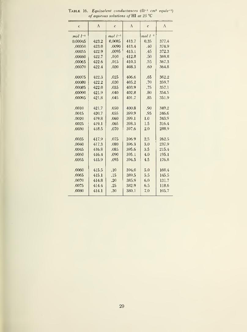
Table 16. Equivalent conductances (fl_1 cm 2 equiv~ l
)
of aqueous solutions of HI at 25 °C
c A c A c A
mol l~ l
0.00045 423.2
mol l~ x
0.0085 413.7
mol l~ x
0.35 377.4
.00050 423.0 .0090 413.4 .40 374.9
.00055 422.9 .0095 413.1 .45 372.3
.00060 422.7 .010 412.8 .50 369.8
.00065 422.6 .015 410.3 .55 367.3
.00070 422.4 .020 408.3 .60 364.8
.00075 422.3 .025 406.6 .65 362.2
.00080 422.2 .030 405.2 .70 359.7
.00085 422.0 .035 403.9 .75 357.1
.00090 421.9 .040 402.8 .80 354.5
.00095 421.8 .045 401.7 .85 351.9
.0010 421.7 .050 400.8 .90 349.2
.0015 420.7 .055 399.9 .95 346.6
.0020 419.8 .060 399.1 1.0 343.9
.0025 419.1 .065 398.3 1.5 316.4
.0030 418.5 .070 397.6 2.0 288.9
.0035 417.9 .075 396.9 2.5 262.5
.0040 417.3 .080 396.3 3.0 237.9
.0045 416.8 .085 395.6 3.5 215.4
.0050 416.4 .090 395.1 4.0 195.1
.0055 415.9 .095 394.5 4.5 176.8
.0060 415.5 .10 394.0 5.0 160.4
.0065 415.1 .15 389.5 5.5 145.5
.0070 414.8 .20 385.9 6.0 131.7
.0075 414.4 .25 382.9 6.5 118.6
.0080 414.1 .30 380.1 7.0 105.7
29

TABLE 17. Equivalent conductances (Vi1 cm 2 equiv *) of aqueous solutions of HI from —20 to 50°
C
c -20 °C -10 °C 0 °C 10 °C 20 °C 30 °C 40 °C 50 °C
mol l~ l
0.4 253.9 300.7 354.5 411.9 453.6 501.8
0.6 249.1 293.6 344.6 401.1 441.5 488.4
0.8 242.4 285.5 333.9 389.1 429.3 474.8
1.0 234.8 276.9 322.7 376.3 416.5 460.8
1.2 226.6 267.9 311.4 363.1 403.4 446.3
1.4 218.2 258.8 300.2 349.8 390.0 431.4
1.6 209.9 249.7 289.1 336.6 376.5 416.3
1.8 201.8 240.7 278.4 323.7 363.0 401.2
2.0 194.0 231.9 268.1 311.1 349.6 386.1
2.2 147.7 186.6 223.4 258.2 299.0 336.3 371.2
2.4 143.5 179.5 215.1 248.8 287.3 323.3 356.5
2.6 138.8 172.8 207.2 239.7 276.1 310.5 342.2
2.8 133.9 166.5 199.5 231.0 265.4 298.1 328.2
3.0 99.9 129.0 160.5 192.0 222.7 255.1 286.1 314.7
3.2 97.4 124.1 154.7 184.8 214.6 245.2 274.5 301.7
3.4 94.2 119.5 149.1 177.8 206.7 235.7 263.4 289.2
3.6 90.6 115.0 143.7 171.0 198.9 226.4 252.6 277.3
3.8 86.9 110.9 138.3 164.3 191.2 217.4 242.3 266.0
4.0 83.6 106.9 132.8 157.6 183.5 208.4 232.5 255.3
4.2 80.9 103.0 127.3 151.0 175.6 199.6 223.1 245.3
4.4 79.3 99.2 121.6 144.3 167.5 190.7 214.1 235.9
30

Table 18. Interpolation formulas for A for HI "• d - e
t°C-20 A =— 188.5 + 268.0c - 79.17c 2 + 7.294c 3
-10 A = 55.399 + 157.67c - 82.804c 2 + 16.276c 3 - 1 . 1560c 4
0 A = 266.31 - 88.70c'/2 + 280.455c - 370.407c 3/ 2 + 176.385c 2 - 29.2746c 5 / 2
10 A = 330.58 - 1 15.18c'/ 2 + 248.768c - 298.965
c
3/2 + 132.508c 2 - 20.8142c 5 /2
20 A = 394.66 - 143.70c'/2 + 302.982c - 379.036c 3/2 + 177.129c 2 - 29.2963c 5'2
» 25 A = 426.45 - 158.72c'/ 2 + 185.96c log c + 1085.7c - 11678c 3/ 2 + 107071c 2 - 394591c 5/ 2
c 25 A = 426.45 - 158.72c'/ 2 + 248.885c - 256.566
c
3'2 + 96.2195c 2 - 12.3887c 5 /2
30 A = 457.93 - 174.20c'/ 2 4- 370.263c - 445.069c 3/2 + 198.665c 2 - 31.2569c5/2
40 A = 519.72 - 206.42c'/2 + 317.597c - 312.945c 5/2 + 112.255c 2 - 13.6656c 5/2
50 A = 579.38 - 240.28c'/ 2 + 354.327c - 331 . 163c 5/2 + 1 10.209c 2 - 1 1.7132c 5/2
a The c log c term was not used for temperatures other than 25 °C because data were not
available below 0.4N.
» 0.0000- 0.01 N.c 0.01N— 7.ON.d The dimensions of the coefficients are such that their product with the c quantity is fl
_1
cm 2 equiv -1.
e Statistical Information.
t °c s n Standarderror
-20 0.07 5 0.03
-10 .14 7 .05
0 1.05 15 .3
10 .75 15 .2
20 1.63 15 .4
25 1.03 30 .2
30 1.14 12 .3
40 1.40 13 .4
50 2.38 13 .6
Table 19. Limiting equivalent conductances
{n~'cm2>equiv~ 1 )of HF, HC1, HBr andWl in water at 25 °C
Thispaper
Maclnnes[64]*
Harnedand Owen
[65]*
Robinsonand Stokes
[66]*
HF 405.10
25 °C
405.01
HC1 426.06 425.95 425.94 425.9.5
HBr 427.74 428.0, 427. 7» 427.7 4
HI 426.45 426A 426.4» 426.44
*Values converted to absolute electrical units.
31

14. Glossary of Symbols
a, activity; also ion size, “ion-size” parameter, or
“distance of closest approach” of ions.
b, Bjerrum ion parameter in conductance (see
eq. (5.10)).
c, concentration in equivalents per 1000 cm 3.
d, density.
e, elementary charge.
i, electric current.
ji, j[, j-2 , j2 , constants in the expression relating Afor HF with the concentration of HF (see p. 10).
k, Boltzmann constant; also constant relating the
equilibrium between HF7 and HF and F~(see table 9).
k,, general forces acting on ions.
A's ,general forces acting on solvent molecules.
/, length in cm; liter.
m, molar concentration.
m' , ionic mobility coefficient.
m, meter.
n, localized average concentration of ions.
rii, number of i ions per volume V.
riji ,average concentration of i ions in the vicinity
of j ions.
q , function in theory of conductance (see p. 5).
r, distance of separation of charges,
ri, unit vector.
Sj-, standard deviations for equation fits.
t, transference or transport number; temperature.
u, ionic mobility.
u°, limiting ionic mobility.
uf, “absolute” mobility of an ion.
u\, “electrical ionic mobility.”
v, velocity.
y, ratio of the concentration of F~ to the stoichio-
metric concentration of HF.73 , ratio of the concentration of HF 2 to the stoichio-
metric concentration of HF.z\ ,
ionic charge.
A , area in cm 2.
A', A", integration constants (see equation (A. 11 )).
A c , coefficient in the limiting law of Debye andHiickel for activity coefficients, on molar basis
(see table 7).
A, B, C, D, E, F, G, constants in polynomials.
B\, coefficient of the relaxation term in the theory
of conductance (see table 3).
By, coefficient of the electrophoretic term in the
theory of conductance (see table 3).
B r , coefficient of ion-size term in the Debye-Hiickeltheory for activity coefficients, on molar scale
(see table 7).
C, stoichiometric concentration.
E, constant in Fuoss-Onsager theory of conductance.
Ei, constant needed to calculate E (see table 4).
E 2 ,constant needed to calculate E (see table 4).
E„, applied potential.
F, Faraday.
/, ionic strength.
J(a), coefficient of c term in the Fuoss-Onsager
theory of conductance.
Jr, cell constant.
K, dissociation constant.
K\, association constant.
K°a, association constant including effects of solute-
solvent interactions and the free volume of the
solute.
L(a), coefficient of the c term in the Fuoss-Onsager-Skinner theory of conductance.
M, molarity.
N, Avogadro constant.
Nj, number of i ions.
r b
Q{b), the definite integral exp {x)x Adx where
x = e 2lrekT.
R, electrical resistance.
R sp , specific electrical resistance or electrical
resistivity.
S, constant equal to B\Ao + B’.
T, Kelvin temperature.
U, potential energy.
V, volume.W, function in the theory of conductance and
related to q (see page 17).
X, vector electric field in the x-direction.
force.
electrical force.
a, degree of dissociation or ionization or complex
formation.
1—a, degree of association.
7 . activity coefficient,
e. dielectric constant,
to, permittivity of free space.
r\, viscosity.
Tjo, viscosity of solvent.
k, the reciprocal of the average radius of an ionic
atmosphere.cr, electrical conductance.
crsp ,specific electrical conductance or electrical
conductivity.
(crsp)s, standard specific electrical conductivity.
cr p , electrical conductance of an experimental
solution.
X, ionic equivalent conductance.
A„, limiting ionic equivalent conductance.
v, number of ions in one molecule ot electrolyte.
p r , charge density.
Pi, coefficient of ionic friction.
r, relation of the Bjerrum parameter and 1 Ik.
A, equivalent conductance.
Ao, limiting equivalent conductance.
A'", molar conductance.A,"', limiting molar conductance.
O, function of volume (see p. 14).
VF\ electric potential.
32


-

Announcement of New Publications in
National Standard Reference Data Series
Superintendent of Documents,
Government Printing Office,
Washington, D.C. 20402
Dear Sir:
Please add my name to the announcement list of new publications to be issued
in the series: National Standard Reference Data Series — National Bureau of
Standards.
Name
Company
Address
City State Zip Code
(Notification key N-337)

.
-

(cut
here)
Publications in the National Standard Reference Data Series
National Bureau of Standards
You may use this listing as your order form by
checking the proper box of the publication(s) youdesire or by providing the full identification of the
publication you wish to purchase. The full letter
symbols with each publications number and full
title of the publication and author must be given
in your order, e.g. NSRDS-NBS-17, Tables of
Molecular Vibrational Frequencies, Part 3, by T.
Shimanouchi.Pay for publications by check, money order, or
Superintendent of Documents coupons or deposit
account. Make checks and money orders payable
to Superintendent of Documents. Foreign remit-
NSRDS-NBS 1, National Standard Reference Data System-Plan of Operation, by E, L. Brady and M. B. Wallenstein, 1964
(15 cents).
NSRDS-NBS 2, Thermal Properties of Aqueous Uni-univalent
Electrolytes, by V. B. Parker, 1965 (45 cents).
NSRDS-NBS 3, Sec. 1, Selected Tables of Atomic Spectra,
Atomic Energy Levels and Multiplet Tables, Si II, Si III, Si IV,
by C. E. Moore, 1965 (35 cents).
NSRDS-NBS 3, Sec. 2, Selected Tables of Atomic Spectra,
Atomic Energy Levels and Multiplet Tables, Si I, by C. E.
Moore, 1967 (20 cents).
NSRDS-NBS 4, Atomic Transition Probabilities, Volume 1,
Hydrogen Through Neon, by W. L. Wiese, M. W. Smith and
B. M. Glennon, 1966 ($2.50).
NSRDS-NBS 5, The Band Spectrum of Carbon Monoxide, by
P. H. Krupenie, 1966 (70 cents).
NSRDS-NBS 6, Tables of Molecular Vibrational Frequencies,
Part 1, by T. Shimanouchi, 1967 (40 cents).
NSRDS-NBS 7, High Temperature Properties and Decomposi-
tion of Inorganic Salts, Part 1, Sulfates, by K. H. Stern and
E. L. Weise, 1966 (35 cents).
NSRDS-NBS 8, Thermal Conductivity of Selected Materials, by
R. W. Powell, C. Y. Ho, and P. E. Liley, 1966 ($1.00).
NSRDS-NBS 9, Bimolecular Gas Phase Reactions (rate coeffi-
cients), by A. F. Trotman-Dickenson and G. S. Milne, 1967
($2 .00 ).
NSRDS-NBS 10, Selected Values of Electric Dipole Moments
for Molecules in the Gas Phase, by R. D. Nelson, Jr., D. R.
Lide, Jr., and A. A. Maryott, 1967 (40 cents).
NSRDS-NBS 11, Tables of Molecular Vibrational Frequencies,
Part 2, by T. Shimanouchi, 1967 (30 cents).
NSRDS-NBS 12, Tables for the Rigid Asymmetric Roto: Trans-
formation Coefficients from Symmetric to Asymmetric Bases
and Expectation Values of P*, PJ, and P®, by R. H. Schwende-
man, 1968 (60 cents).
NSRDS-NBS 13, Hydrogenation of Ethylene on Metallic Cata-
lysts, by J. Horiuti and K. Miyahara, 1968 ($1.00).
NSRDS-NBS 14, X-Ray Wavelengths and X-Ray Atomic Energy
Levels, by J. A. Bearden, 1967 (40 cents).
NSRDS NBS 15, Molten Salts, Vol. 1, Electrical Conductance,
Density, and Viscosity Data, by G. Janz, F. W. Dampier, G. R.
Lakshminarayanan, P. K. Lorenz, and R. P. T. Tomkins, 1968
($3.00).
NSRDS-NBS 16, Thermal Conductivity of Selected Materials,
Part 2, by C. Y. Ho, R. W. Powell, and P. E. Liley, 1968
($2 .00 ).
tances should be made either by international
money order or draft on an American bank.Postage stamps are not acceptable.No charge is made for postage to destinations
in the United States and possessions, Canada,Mexico, and certain Central and South Americancountries. To other countries, payments for docu-ments must cover postage. Therefore, one-fourthof the price of the publication should be added for
postage.
Send your order together with remittance to
Superintendent of Documents, Government Print-
ing Office, Washington, D.C. 20402.
NSRDS-NBS 17, Tables of Molecular Vibration Frequencies,
Part 3, by T. Shimanouchi, 1968 (30 cents).
NSRDS-NBS 18, Critical Analysis of the Heat-Capacity Data
of the Literature and Evaluation of Thermodynamic Prop-
erties of Copper, Silver, and Gold From 0 to 300 K, by G. T.
Furukawa, W. G. Saba, and M. L. Reilly, 1968 (40 cents).
NSRDS-NBS 19, Thermodynamic Properties of Ammonia as
an Ideal Gas, by L. Haar, 1968 (20 cents).
NSRDS-NBS 20, Gas Phase Reaction Kinetics of Neutral
Oxygen Species, by H. S. Johnson, 1968 (45 cents).
NSRDS-NBS 21, Kinetic Data on Gas Phase Unimolecular Re-
actions, by S. W. Benson and H. E. O’Neal (In press).
NSRDS-NBS 22, Atomic Transition Probabilities, Vol. II,
Sodium Through Calcium, A Critical Data Compilation, by
W. L. Wiese, M. W. Smith, and B. M. Miles ($4.50).
NSRDS-NBS 23, Partial Grotrian Diagrams of Astrophysical
Interest, by C. E. Moore and P. W. Merrill, 1968 (55 cents).
NSRDS-NBS 24, Theoretical Mean Activity Coefficients of
Strong Electrolytes in Aqueous Solutions from 0 to 100 °C,
by Walter J. Hamer, 1968 ($4.25).
NSRDS-NBS 25, Electron Impact Excitation of Atoms, by B. L.
Moiseiwitsch and S. J. Smith, 1968 ($2.00).
NSRDS-NBS 26, Ionization Potentials, Appearance Potentials,
and Heats of Formation of Positive Ions, by J. L. Franklin,
J. G. Dillard, H. M. Rosenstock, J. T. Herron, K. Draxl, and
F. H. Field ($4.00).
NSRDS-NBS 27, Thermodynamic Properties of Argon from the
Triple Point to 300 K at Pressures to 1000 Atmospheres, by
A. L. Gosman, R. D. McCarty, and J. G. Hust ($1.25).
NSRDS-NBS 28, Molten Salts, Vol. 2, Section 1, Electro-
chemistry of Molten Salts: Gibbs Free Energies and Excess
Free Energies From Equilibrium-Type Cells, by G. J. Janz and
C. G. M. Dijkhuis. Section 2, Surface Tension Data, by G. J.
Janz, G. R. Lakshminarayanan, R. P. T. Tomkins, and J. Wong
($2.75).
NSRDS-NBS 29, Photon Cross Sections, Attenuation Coeffi-
cients and Energy Absorption Coefficients and Energy
Absorption Coefficients from 10 keV to 100 GeV, by J. H.
Hubbell (75 cents).
NSRDS-NBS 30, High Temperature Properties and Decomposi-
tion of Inorganic Salts, Part 2, Carbonates, by K. H. Stern
and E. L. Weise (45 cents).
NSRDS-NBS 31, Bond Dissociation Energies in Simple
Molecules, by B. deB. Darwent (55 cents).
NSRDS-NBS 32, Phase Behavior in Binary Multicomponent
Systems at Elevated Pressures: n-Pentane and Methane-n-
Pentane, by V. M. Berry and B. H. Sage (In press).
U.S. GOVERNMENT PRINTING OFFICE: 1970 0—372-265

I

NBS TECHNICAL PUBLICATIONS
PERIODICALS
JOURNAL OF RESEARCH reports National
Bureau of Standards research and development in
physics, mathematics, chemistry, and engineering.
Comprehensive scientific papers give complete details
of the work, including laboratory data, experimental
procedures, and theoretical and mathematical analy-
ses. Illustrated with photographs, drawings, andcharts.
Published in three sections, available separately:
• Physics and Chemistry
Papers of interest primarily to scientists working in
these fields. This section covers a broad range of
physical and chemical research, with major emphasis
on standards of physical measurement, fundamentalconstants, and properties of matter. Issued six times
a year. Annual subscription: Domestic, $9.50; for-
eign, $11.75*.
• Mathematical Sciences
Studies and compilations designed mainly for the
mathematician and theoretical physicist. Topics in
mathematical statistics, theory of experiment,' design,
numerical analysis, theoretical physics and chemis-
try, logical design and programming of computers
and computer systems. Short numerical tables.
Issued quarterly. Annual subscription: Domestic,
$5.00; foreign, $6.25*.
• Engineering and Instrumentation
Reporting results of interest chiefly to the engineer
and the applied scientist. This section includes manyof the new developments in instrumentation resulting
from the Bureau’s work in physical measurement,data processing, and development of test methods.It will also cover some of the work in acoustics,
applied mechanics, building research, and cryogenic
engineering. Issued quarterly. Annual subscription:
Domestic, $5.00; foreign, $6.25*.
TECHNICAL NEWS BULLETIN
The best single source of information concerning the
Bureau’s research, developmental, cooperative andpublication activities, this monthly publication is
designed for the industry-oriented individual whosedaily work involves intimate contact with science andtechnology—for engineers, chemists, physicists, re-
search managers, product-development managers, andcompany executives. Annual subscription: Domestic,
$3.00; foreign, $4.00*.
• Difference in price is due to extra cost of foreign mailing.
Order NBS publications from:
NONPERIODICALS
Applied Mathematics Series. Mathematical tables,
manuals, and studies.
Building Science Series. Research results, test
methods, and performance criteria of building ma-terials, components, systems, and structures.
Handbooks. Recommended codes of engineering
and industrial practice (including safety codes) de-
veloped in cooperation with interested industries,
professional organizations, and regulatory bodies.
Special Publications. Proceedings of NBS confer-
ences, bibliographies, annual reports, wall charts,
pamphlets, etc.
Monographs. Major contributions to the technical
literature on various subjects related to the Bureau’s
scientific and technical activities.
National Standard Reference Data Series.
NSRDS provides quantitive data on the physical
and chemical properties of materials, compiled fromthe world’s literature and critically evaluated.
Product Standards. Provide requirements for sizes,
types, quality and methods for testing various indus-
trial products. These standards are developed coopera-
tively with interested Government and industry groups
and provide the basis for common understanding of
product characteristics for both buyers and sellers.
Their use is voluntary.
Technical Notes. This series consists of communi-cations and reports (covering both other agency andNBS-sponsored work) of limited or transitory interest.
Federal Information Processing Standards Pub-lications. This series is the official publication within
the Federal Government for information on standards
adopted and promulgated under the Public Law89—306, and Bureau of the Budget Circular A—86entitled, Standardization of Data Elements and Codesin Data Systems.
CLEARINGHOUSE
The Clearinghouse for Federal Scientific andTechnical Information, operated by NBS, supplies
unclassified information related to Government-gen-
erated science and technology in defense, space,
atomic energy, and other national programs. For
further information on Clearinghouse services, write:
Clearinghouse
U.S. Department of CommerceSpringfield, Virginia 22151
Superintendent of DocumentsGovernment Printing Office
Washington, D.C. 20402

![$m mi fm - NISTnvlpubs.nist.gov/nistpubs/Legacy/NSRDS/nbsnsrds28.pdfTheparticipationofT.G.Coker,F.W.Dampier,P.K.Lorenz,H.Siegenthaler, ... FFaradayConstant TTemperaturein°K ... oftheTemkinrelation[8]](https://img.pdfslide.us/doc/110x75/5ac385f77f8b9a57528c3245/m-mi-fm-fwdampierpklorenzhsiegenthaler-ffaradayconstant-ttemperatureink.jpg)