A Customer-Item Decomposition Approach to Stochastic

Inventory Systems with Correlation

Yimin Yu • Saif Benjaafar

Graduate Program in Industrial and Systems Engineering

Department of Mechanical Engineering

University of Minnesota, Minneapolis, MN 55455

yimin@me.umn.edu, saif@umn.edu

November 2006, Revised January 2008

Abstract

We consider an inventory system with a single stage, periodic review, correlated, non-stationary

stochastic demand and correlated, non-stationary stochastic and sequential leadtimes. We use

the customer-item decomposition approach to decompose the problem into sub-problems, each

involving a single customer-item pair. We then formulate each subproblem as an optimal stop-

ping problem. We use properties that arise from this formulation to show that the optimal

policy is a state-dependent base-stock policy and to show, for several cases, that the optimal

policy can be obtained via a polynomial time algorithm. We also use the formulation to con-

struct a myopic heuristic which leads to an explicit solution for the optimal policy in the form

of a critical fractile. We characterize conditions under which the myopic heuristic is optimal.

Key words: Stochastic inventory systems, demand correlation, leadtime correlation, optimal

control, optimal stopping problem, myopic policy

1

1 Introduction

A common assumption in the inventory literature is that demands and leadtimes are independent

across review periods and independent of external events. In practice, this is rarely the case.

Demands is often correlated over time. Factors that influence an increase or decrease in demand in

one period often persist over the next few periods. In fact, the presence of time-correlation is what

makes demand forecasting a meaningful activity. Demand is also often correlated with external

events. For example, inflation levels, levels of employment, and interest rates tend to significantly

affect consumption and, consequently, demand for most products. Similarly, correlated leadtimes

are common in practice. For example, a long leadtime from a supplier in one period often leads to

long leadtimes from that same supplier in the next few periods (if that supplier is backlogged or

experiencing production difficulties). Similarly, external events, such as disruptions to the supply

network, often affect the length of leadtimes over multiple periods.

The relatively limited treatment of correlation in the literature appears to be due to the math-

ematical and computational intractability of the problem. Traditional approaches to the problem,

which rely on dynamic programming and use aggregate information about demand and inventory,

tend to lead to problems with too many dimensions, making them difficult to analyze and solve. In

this paper, we explore an alternative approach based on the so-called customer-item decomposition

method. In this approach, demand is viewed as consisting of a stream of individual customers ar-

riving over time, with a batch of such customers arriving in each period. Inventory (both in-stock,

on-order, and yet to be ordered) is also viewed as a stream of individual items that are delivered

over time, with a batch of such items delivered in each period. Each item is then matched to a

customer. This reduces the inventory control problem to making decisions about when to place an

order for the item destined to a particular customer. This decision can be made, in some cases, by

taking into account only the marginal cost associated with each customer-item pair. In turn, this

decomposes the problem into independent sub-problems, one for each single customer-item pair.

The approach appears to have its origin in a paper by Axsater (1990) and was subsequently

used by Axsater (1993), Katircioglu and Atkins (1998), Muharremoglu and Tsitsiklis (2003), and

Janakiraman and Muckstadt (2005). Axsater considers a two-stage distribution system that oper-

2

ates under a heuristic policy of one-for-one replenishment with fixed base-stock levels. He evaluates

the cost associated with each customer-item pair and uses this to optimize the parameters of the

heuristic (the base-stock levels at each location). Axsater (1993) extends this technique to systems

with batch-ordering and uses it to optimize the parameters of a heuristic based on a reorder point-

reorder quantity policy. Katircioglu and Atkins (1998) study a continuous review system with

arbitrary order inter-arrival time distributions with increasing failure rates and argue that a time-

delayed base-stock policy is optimal. Muharremoglu and Tsitsiklis (2003) study an uncapacitated,

serial systems under periodic-review with Markov-modulated demand and Markov modulated se-

quential leadtimes. They show that a state-dependent base-stock policy is optimal. Janakiraman

and Muckstadt (2005) consider a capacitated two-stage system and use the decomposition approach

to show that the optimal policy is a modified state-dependent base-stock policy.

In this paper, we consider a system with periodic review where both demands and leadtimes are

stochastic and correlated across periods and with external indicators. The demand and leadtime

correlation models we consider are general and incorporate most models treated in the literature,

including Markov-modulated processes, as special cases. We also allow for the cost parameters to

be non-stationary. This is a complex problem for which it is difficult to compute the optimal policy

using a traditional dynamic programming approach and to characterize the structure of an optimal

policy.

We use the customer-item decomposition approach to show how the inventory control problem

can be formulated as a set of independent optimal stopping problems. We then use properties

that arise from this formulation to characterize the structure of the optimal policy, which we show

to be a state-dependent base-stock policy. Our formulation leads, in several important cases, to

polynomial time algorithms. We also use the formulation to construct a myopic heuristic. This

myopic heuristic leads to explicit solutions for the ordering time of each item (or equivalently the

ordering quantity in each period) in the form of a critical fractile. We characterize conditions

under which the myopic policy is optimal and show that these conditions hold for certain classes

of problems.

The rest of this paper is organized as follows. In Section 2, we provide a brief review of related

literature. In Section 3, we describe our approach in the context of the simpler case of inventory

3

systems with independent demands and fixed leadtimes. We do so for ease of exposition and also

because some of the results we present for this simpler case are new. More importantly, we do

it to illustrate the fact that the analysis of systems with stochastic leadtimes and correlation is

not much more complicated (under the decomposition approach) than the analysis of systems with

no correlation. In section 4, we discuss the one-period look-ahead policy (the myopic policy). In

Section 5, we present our main results for systems with stochastic leadtimes and correlation. In

Section 6, we provide some concluding comments and potential future research directions.

2 Related Literature

Our paper is related to two streams in the inventory literature, one dealing with demand correlation

and the other with leadtime correlation. Existing literature that deals with demand correlation

focuses on either characterizing the structure of optimal policies in specific settings or evaluating

the performance of heuristics (sub-optimal policies). A sub-stream within this literature considers

systems with Markov-modulated demand, where demand is stochastic and affected (modulated) by

an exogenous Markov process; see for example, Song and Zipkin (1992, 1993, 1996a), Chen and

Song (2001), Muharremoglu and Tsitsiklis (2003) and the references therein. An important result

from this literature is the optimality of state-dependent base-stock policies.

Another stream within this literature considers demand correlation across periods (time-correlated

demand) for the purpose of modeling inventory systems with forecasting. This includes treatments

with simple time-series models such as the order-one autoregressive process AR(1) in Scarf (1959,

1960), Johnson and Thompson (1975), Erkip et al. (1990), and Lee et al. (1997, 1999), among

others, or more general models such as the Martingale model of forecast evolution (MMFE) intro-

duced by Graves et al. (1986, 1998) and Heath and Jackson (1994), and the random walk model of

Graves (1999) and Lee and Whang (1998). Levi et al. (2005) consider a general model for demand

correlation (we use a similar model in Section 5.2) and then use it to propose a heuristic with

certain performance guarantees.

Papers that study heuristics include the early papers by Veinott (1963, 1965a and 1965b) and

Ignall and Veinott (1969), and more recent ones by Iida and Zipkin (2006), Dong and Lee (2003),

4

Lu et al. (2006), among several others. An important focus of this literature is the evaluation of

so-called myopic heuristics where in each period the objective is to minimize the expected cost for

that period, ignoring the effect on the cost of future periods. Myopic policies have been shown to

be optimal in some cases (See Karlin 1960,Veinott 1965a and 1965b, Johnson and Thompson 1975,

Iida and Zipkin 2006, et al. 2006). Variations on these policies have also been shown to provide

useful bounds (Levi et al. 2005).

The literature on correlated stochastic leadtimes is relatively limited. Song and Zipkin (1996b)

studied a single stage system with Markov modulated leadtimes and Muharremoglu and Tsitsiklis

(2003) studied a serial system with both Markov modulated demand and Markov modulated lead-

times. The optimal policy is shown to be a base-stock policy with the basestock levels dependent

on the state of the modulating Markov process. Markov modulated leadtimes is a special case of

the leadtime correlation we consider in this paper.

Relative to the existing literature, our paper makes the following contributions. It appears to be

the first to provide results regarding the structure of the optimal policy for systems with stochastic

demands and leadtimes, non-stationary cost parameters, and correlation in both demands and

leadtimes. We do so under a general correlation model that includes correlation across periods

and with external indicators. We provide a new approach for proving the structure of the optimal

policy that takes advantage of the optimal stopping problem formulation of the customer-item

subproblems. The approach, which relies on a submodularity result for the marginal expected

cost, is simple and direct. The formulation also gives rise to efficient solution algorithms in several

important cases. The formulation allows us also to easily specify a myopic policy in terms of a

critical fractile. We show that this myopic policy is optimal in several cases. For these cases, our

results appear to be the first to provide an explicit solution for the optimal policy in systems with

general demand correlation.

5

3 Inventory Systems with Independent Demands and Fixed Lead-

times

Consider a single stage inventory problem with multiple periods, stochastic demands, and fixed

deterministic lead times. Demand Dt ≥ 0 in each period t is a discrete random variable with E[Dt] <

∞, where t = 0, · · · , T and T determines the length of the planning horizon. Demands in different

periods are independent but not necessarily identically distributed (i.e., demand distribution can

be time-varying). Inventory is replenished from an outside supplier with a fixed leadtime, L, so

that an item ordered in period t is received in period t + L. We assume that the outside supplier

has ample stock. Demand is satisfied from on-hand inventory, if any is available; otherwise it is

backlogged. In each period, the decision maker must decide on how many units to order to minimize

the expected discounted cost over the entire planning horizon. There are three types of cost: (1)

an ordering cost ct per unit ordered in period t, (2) a holding cost ht per unit of inventory held in

period t and (3) a backorder cost bt for each order that stays backlogged in period t. Note that we

allow for the cost parameters, ht, bt and ct, to be time-varying. All costs for period t are incurred

at the end of period t. Also, without loss of generality, we assume that hT = bT = 0.

We assume that there is no speculative motivation for holding inventory or backlogging orders.

Therefore, we assume that the following conditions on the cost parameters are satisfied.

Assumption 1

βtct + βt+Lht+L > βt+1ct+1, for t = 0, · · · , T − L, (1)

and

βtct < βt+1ct+1 + βt+Lbt+L, for t = 0, · · · , T − L, (2)

where β ∈ (0, 1] is the discount factor.

This assumption is not necessary for our analysis. It is only used in Theorem 2 below to show that

the optimal base-stock level is non-negative and finite. This avoids anomalous behavior such as

6

ordering an infinite amount in some period or not placing orders despite the presence of backorders.

The following describes the sequence of events in each period t, t = 0, · · · , T : first, an order

of size qt is placed with the outside supplier, qt ∈ {0, 1, · · · }, then the order placed in period

t − L (of size qt−L) is received, and finally demand for the current period in the amount of dt is

realized. Holding and backorder costs are incurred at the end of the period. Let INt denote the

net inventory at the beginning of period t, where INt = It−Bt, It is the level of on-hand inventory,

and Bt is the number of backorders. Then INt+1 = INt + qt−L − dt, It = IN+t ≡ max(0, INt) and

Bt = IN−t ≡ max(0,−INt). The holding cost incurred in period t is htIN+

t+1 and the backorder

cost is btIN−t+1 (we assume that costs are charged based on the ending net inventory in period

t which is the same as the starting net inventory in period t + 1) . Finally, let IOt denote the

number of units on order, and IPt denote the inventory position at the beginning of period t, where

IPt ≡ INt + IOt.

The above problem is typically formulated as a stochastic dynamic program, where in each

period t the decision variable is qt, and the state of the system is IPt (IPt = IPt−1 + qt−1 − dt−1).

In this paper, we take a different approach, the customer-item decomposition approach. We view

demand as a stream of individual customers with a batch of such customers arriving in each period

and where each customer requests one unit of the product. To differentiate between the customers,

we assign at the beginning of the planning horizon a unique index i, i = 1, 2, · · · , to each customer

in increasing order of the customers’ arrival times. This means that customer i refers to the ith

customer that will arrive to the system, with ties broken arbitrarily. At any time, the arrival

times of future customers are of course not known. However, we can use knowledge of the demand

distributions at period t to assign a probability pit,s to customer i if the customer has not arrived

yet, where pit,s denotes the probability evaluated at the beginning of period t that the ith customer

will arrive in period s. More specifically, given that k customers have already arrived prior to

period t, we have:

pit,s =

i−k−1∑

n=0

P (Dt + · · · + Ds−1 = n)P (Ds ≥ i − n − k) , s ≥ t (3)

for i > k. If∑T

s=t pit,s < 1, we can simply redefine pi

t,T ≡ 1−∑T−1

s=t pjt,s, since the customer arrivals

7

at period T will not affect system costs 1. Thus, we have∑T

s=t pit,s = 1 (recall that we assume

hT = bT = 0)

Similarly, we view supply as a stream of physical items with a batch of such items delivered

in each period. We assign index j ′, j′ = 1′, 2′, · · · , to each item in increasing order of the items’

delivery times, with ties again broken arbitrarily. We refer the jth item as item j ′. The delivery

times of items are obviously determined by when orders are placed with the outside supplier.

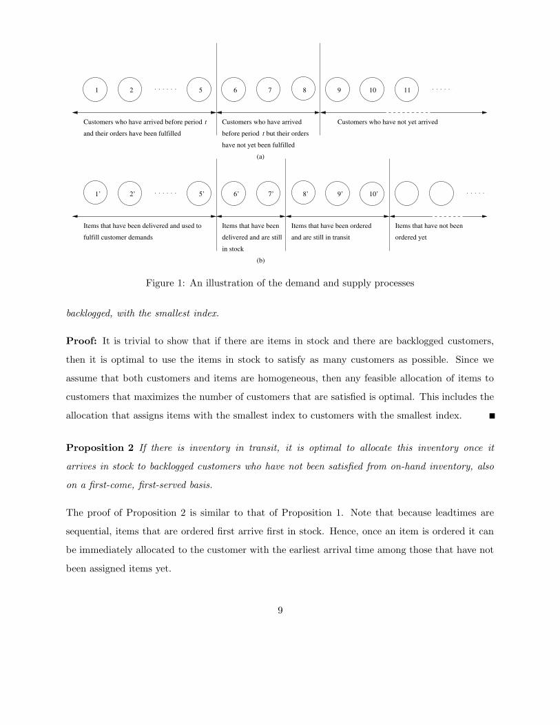
At the beginning of a period t, some customers would have already arrived to the system and

their orders fulfilled; some customers would have arrived but their orders would have not been

fulfilled (they are currently backlogged), while the remaining customers would have not arrived

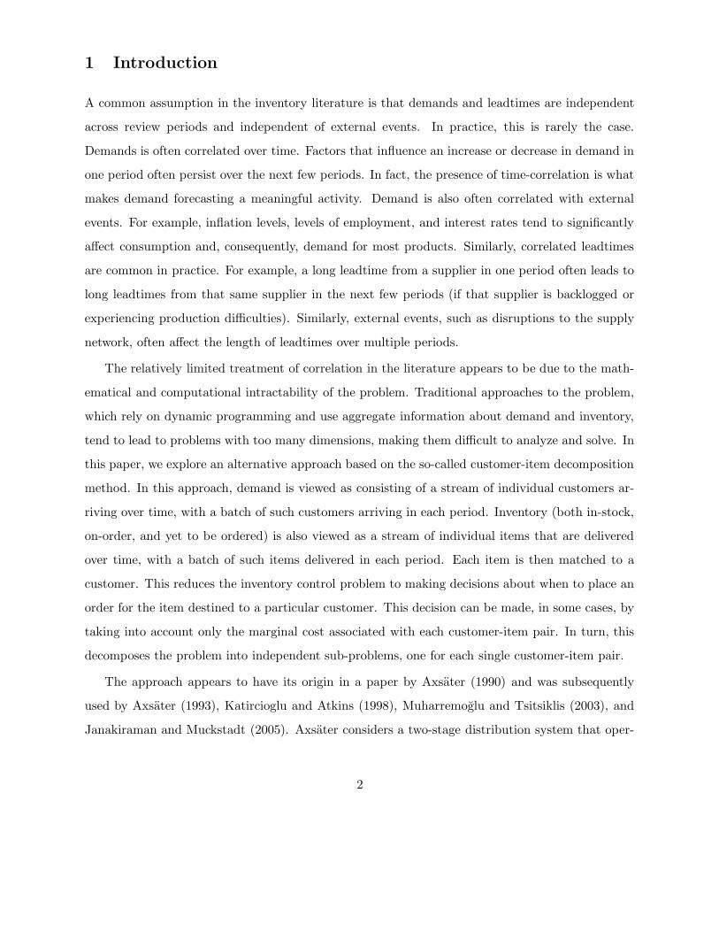
yet. This situation is graphically depicted in Figure 1. Similarly, at the beginning of the same

period, some items would have been delivered and used to fulfill customer orders, some items

would be in transit (they were ordered some time after t−L), some items would be in stock, while

the remaining items (potentially an infinite number of them) would have not been ordered yet; see

Figure 1 for an illustration.

The inventory control problem can now be restated for each period in terms of (1) determining

which items to order, among those who have not been ordered yet and (2) determining how to

allocate available stock to customers who have arrived but whose orders have not been fulfilled yet.

More specifically, at the beginning of each period, we must first decide on how many additional

items to order from the outside supplier (this is equivalent to determining the order quantity), we

then observe the delivery of items, ordered L periods ago, and the arrival of new customers, we

finally must decide on how to allocate items in stock to customers who have arrived but whose

orders have not been fulfilled yet. This includes customers who have arrived in the current period

as well as any backlogged from previous periods.

Proposition 1 If there is inventory on-hand, it is optimal to use this inventory to satisfy customers

that are currently backlogged. Moreover, it is optimal to allocate this inventory on a first-come,

first-served basis, so that the item with the smallest index is assigned to the customer, among those

1Formally, we can define a random variable Xi to describe the arrival time of customer i, where Xi corresponds

to the smallest integer 0 ≤ s ≤ T such that D0 + · · ·+ Ds ≥ i, with Xi = T if no such s exists. The probabilities pit,s

characterize the distribution of Xi given the demand realizations in periods 0, ..., t − 1.

8

2 5

and their orders have been fulfilled

1

Customers who have arrived

have not yet been fulfilled

Customers who have not yet arrived

1’ 5’

6 7 8 9 10 11

7’ 8’ 9’ 10’

(a)

Items that have been delivered and used tofulfill customer demands

Items that have beendelivered and are stillin stock

Items that have been orderedand are still in transit

Items that have not been ordered yet

(b)

2’ 6’

Customers who have arrived before period ttbefore period but their orders

Figure 1: An illustration of the demand and supply processes

backlogged, with the smallest index.

Proof: It is trivial to show that if there are items in stock and there are backlogged customers,

then it is optimal to use the items in stock to satisfy as many customers as possible. Since we

assume that both customers and items are homogeneous, then any feasible allocation of items to

customers that maximizes the number of customers that are satisfied is optimal. This includes the

allocation that assigns items with the smallest index to customers with the smallest index.

Proposition 2 If there is inventory in transit, it is optimal to allocate this inventory once it

arrives in stock to backlogged customers who have not been satisfied from on-hand inventory, also

on a first-come, first-served basis.

The proof of Proposition 2 is similar to that of Proposition 1. Note that because leadtimes are

sequential, items that are ordered first arrive first in stock. Hence, once an item is ordered it can

be immediately allocated to the customer with the earliest arrival time among those that have not

been assigned items yet.

9

Propositions 1 and 2 show that once an item has been ordered, it is optimal to immediately

commit it to the customer with the earliest arrival time among those who have not been assigned

items yet. Consider now an extension of this allocation policy where we commit all items to specific

customers whether or not they have been ordered. We will show that such a policy is indeed optimal.

In order to do so, we will show that it leads to assigning items once they have been ordered to

customer on a first-come, first-served basis.

Suppose that at the beginning of period 0, there are k items that have already been ordered and

are either in transit or in stock, then by the virtue of Proposition 1 and Proposition 2, we know

that it is optimal to allocate these k items to the first k customers on a first-come, first-served

basis. For each of the other customers, let us also assign an item (yet to be ordered) to which we

will refer as item a(i) for i = k + 1, k + 2, · · · . This is possible since the outside supplier can be

viewed as maintaining an infinite stock of items. These items are, by assumption, homogeneous and

undifferentiated prior to ordering. Hence, we can couple each item with the supplier to a specific

customer. By coupling a specific item to a specific customer, we are committed to allocating the

item to the customer regardless of when the item would eventually be ordered and regardless of

when the customer would eventually arrive. We refer to this allocation policy as the committed

allocation policy (see also Muharremoglu and Tsitsiklis 2003 for a similar notion). Since under a

committed allocation policy there is a one-to-one correspondence between customers and items, we

can use a single index, say i, to refer to a coupled customer-item pair i, so that item a(i) now refers

to the item that is allocated to customer i.

Given a committed allocation policy, the inventory control problem reduces to making decisions

in each period on whether or not we should order an item a(i) (destined for customer i) if the item

has not been ordered yet to minimize the expected cost incurred by each customer-item pair. Note

that the expected cost associated with an ordering decision depends only on the distribution of

arrival time Xi of customer i. To see why this is the true, let us consider the case where Xi = xi,

where xi is a particular realization of the arrival time random variable Xi. Also, let τa(i) be the

time at which item a(i) is ordered. If τa(i) + L < xi (the item is delivered before its corresponding

10

customer arrives), then the system incurs a holding cost

g(τa(i), xi) =

xi−1∑

k=τa(i)+L

βkhk; (4)

if τa(i) + L = xi, (the item is delivered in the same period the customer arrives), no holding nor a

backorder cost is incurred; while if τa(i) +L > xi, (the customer arrives before its item is delivered),

the system incurs a backorder cost

g(τa(i), xi) =

τa(i)+L−1∑

k=xi

βkbk. (5)

As we can see, although the dynamics of different customers are correlated (i.e., knowing the ar-

rival of customer j will give us new information concerning customer j +1), the marginal inventory

cost due to a customer-item pair, depends only on when the item is ordered and when the cus-

tomer arrives and is independent of ordering decisions made for other customer-item pairs under a

committed allocation policy.

The expected marginal cost, evaluated in period t, of ordering item a(i) in period l = t, · · · , T −

L − 1 is given by

Gl(i|Ht−1) = βlcl +l+L−1∑

s=t

pit,s

l+L−1∑

k=s

βkbk +T∑

s=l+L+1

pit,s

s−1∑

k=l+L

βkhk. (6)

where Ht−1 = (d0, · · · , dt−1) is the vector of realized demand in periods 0, · · · , t−1, and represents

the information set available at time t (note that the probabilities pit,s depend on Ht−1). The first

term on the right-hand side of the above equality is the discounted ordering cost associated with

ordering item a(i) in period l. The second term is the expected backorder cost and the third term

is the expected holding cost. A backorder cost is incurred if customer i arrives in a period s such

that t ≤ s < l + L. The corresponding cost is then∑l+L−1

k=s βkbk, and the expected cost over all

possible values of s is∑l+L−1

s=t pit,s

∑l+L−1k=s βkbk. A holding cost is incurred if customer i arrives in

a period s such l + L < s. The corresponding cost is then∑s−1

k=l+L βkhk and the expected cost is∑T

s=l+L+1 pit,s

∑s−1k=l+L βkhk.

11

In every period t, we must decide whether or not to place an order for item a(i), if it is has not

been ordered already. In making this decision, we compare the expected cost of ordering the item

in period t to the cost of postponing the ordering decision until a later period. Hence, the ordering

decision can be formulated as an optimal stopping problem (in an optimal stopping problem, the

decision is when to terminate a process by taking a certain action, which in our case corresponds

to placing an order). The optimality equation in period t is given by

Vt(i|Ht−1) = min{Gt(i|Ht−1), E[Vt+1(i|Ht)]}, (7)

for t = 0, · · · , T − L − 1, so that it is optimal to order in period t if Gt(i|Ht−1) ≤ E[Vt+1(i|Ht)]

and to postpone the decision otherwise. Note that the expectation in (7) is taken with respect to

demand in period t, Dt.

Since under a committed allocation policy, the cost incurred by a particular customer-pair

depends only on when the item is ordered and when the customer arrives and is independent of

ordering decisions made for other customer-item pairs, the decision for each item can be treated

independently of decisions for other items. This immediately leads to the following result.

Proposition 3 Under a committed allocation policy, the ordering decision for each customer-item

pair can be made independently of decisions for other customer-item pairs.

The following proposition is needed for the proof of Theorem 1 .

Proposition 4 The function Gl(i|Ht−1) is submodular in (l, i) for t = 0, ..., T , l ≥ t and all

customers i ≥ 1 whose items have not already been ordered at the beginning of period t. That is,

Gl(i|Ht−1) − Gl+1(i|Ht−1) ≤ Gl(i + 1|Ht−1) − Gl+1(i + 1|Ht−1)

for all Ht−1 ∈ Ft−1, where Ft is the set of all possible vectors of demand realizations in periods

0, · · · , t.

Proof. First, let us note that for every possible realization xi and xi+1 of the random variables Xi

and Xi+1 respectively, we have xi ≤ xi+1. Therefore, we also have Pr(Xi > a) ≤ Pr(Xi+1 > a)

12

for any a > 0. In other words, Xi is stochastically smaller than Xi+1. Next, let us consider the

difference

Gl+1(i|Ht−1) − Gl(i|Ht−1) = βl+1cl+1 − βlcl + βl+Lbl+L

l+L∑

s=t

pit,s − βl+Lhl+L

T∑

s=l+L+1

pit,s.

Since Xi is stochastically smaller than Xi+1, we have∑T

s=l+L+1 pit,s ≤

∑Ts=l+L+1 pi+1

t,s , and it follows

that

Gl+1(i|Ht−1) − Gl(i|Ht−1) ≥ Gl+1(i + 1|Ht−1) − Gl(i + 1|Ht−1).

Hence, the function Gl(i|Ht−1) is submodular in (i, l).

The submodularity of the function Gl(i|Ht−1) leads to the following important result.

Theorem 1 It is always optimal to order item a(i) for customer i no later than item a(i + 1) for

customer i + 1. That is,

Gt(i|Ht−1) − E[Vt+1(i|Ht)] ≤ Gt(i + 1|Ht−1) − E[Vt+1(i + 1|Ht)]

for all t and all i and all Ht ∈ Ft. Consequently, the committed allocation policy is optimal.

Proof. We prove the result by induction. First note that in period T −L− 1, the optimal decision

is either to order in period T − L − 1 or to order in period T − L (which is equivalent to not

ordering). Hence,

VT−L−1(i|HT−L−2) =min{GT−L−1(i|HT−L−2), E[VT−L(i|HT−L−1)]}

=min{GT−L−1(i|HT−L−2), GT−L(i,HT−L−2)}.

From Proposition 4, we have

GT−L−1(i|HT−L−2) − GT−L(i|HT−L−2) ≤ GT−L−1(i + 1|HT−L−2) − GT−L(i + 1|HT−L−2).

13

Next, suppose that

Gk+1(i|Hk) − E[Vk+2(i|Hk+1)] ≤ Gk+1(i + 1|Hk) − E[Vk+2(i + 1|Hk+1)],

where k < T + L − 2. It follows that

Gk(i|Hk−1) − E[Vk+1(i|Hk)]

=Gk(i|Hk−1) − E[min{Gk+1(i|Hk), E[Vk+2(i|Hk+1)]}]

=Gk(i|Hk−1) − E[Gk+1(i|Hk) + min{0, E[Vk+2(i|Hk+1)] − Gk+1(i|Hk)}]

=Gk(i|Hk−1) − Gk+1(i|Hk−1) − E[min{0, E[Vk+2(i|Hk+1)] − Gk+1(i|Hk)}]

≤Gk(i + 1|Hk−1) − Gk+1(i + 1|Hk−1) − E[min{0, E[Vk+2(i + 1|Hk+1)] − Gk+1(i + 1|Hk)}]

=Gk(i + 1|Hk−1) − E[Vk+1(i + 1|Hk)],

the inequality is due to Proposition 4 and the inductive assumption.

The optimality of the committed allocation policy follows from the fact that the ith item to be

ordered is always assigned to the ith customer to arrive (a(i) = i′), and from Propositions 1 and 2.

In the following theorem, we show that the optimal ordering policy in each period is a base-stock

policy.

Theorem 2 The optimal ordering policy in periods t = 0, · · · , T −L− 1 is a base-stock policy with

base-stock level st, such that if IPt < st, we order st − IPt items and if IPt ≥ st, we order nothing,

where IPt is the inventory position at the beginning of period t. For periods T − L, · · · , T , it is

optimal to order nothing. Moreover, 0 ≤ st < ∞ for t = 0, · · · , T − L − 1.

Proof: First, we show that it is optimal to order items for any customers who are currently

backlogged and whose items have not been ordered yet. Suppose customer i arrived at some period

xi < t (period t is the current period). Consider the marginal cost g(l, xi) = βlcl +∑l+L−1

k=xiβkbk

14

incurred by the system if item a(i) is ordered in some period l ≥ t. Then, it is easy to show that

g(l + 1, xi) − g(l, xi) = βl+1cl+1 − βlcl + βl+Lbl+L > 0,

where the inequality follows from Assumption 1, which implies that it is indeed optimal to order

item a(i) in period t.

Hence, the only non-trivial decision is for how many future customers to place orders at period

t. Suppose that there are k customers have arrived at the beginning of period t. Let k + j ∗(t) be

the index of the largest customer for which it is optimal to order in period t. Because demands in

different periods are independent, this decision is independent of past demand (i.e., the number of

customers who have already arrived). Then j∗(t) is independent of k. The value of j∗(t) is also

independent of past and future ordering decisions since the decision to order for customer k + j ∗(t)

is independent of all other ordering decisions. By virtue of Theorem 1, if it is optimal to order for

customer k + j∗(t), then it is optimal to order items for customers k + 1, k + 2, · · · , k + j∗(t) − 1 if

these items have not been ordered yet in previous periods. This would bring the inventory position

to j∗(t). On the other hand, if the current inventory position is greater than or equal to j ∗(t), then

we order nothing. Hence, the optimal policy is a base-stock policy with base-stock level st = j∗(t).

Because items ordered in periods T − L, · · · , T will not arrive earlier than period T , it is

optimal to order nothing in periods T − L, · · · , T . The fact that we always order enough to bring

the inventory position to zero (we always order items for customers that have arrived) implies that

st ≥ 0. To show that st < ∞, we first note that∑l+L

s=t pk+jt,s → 0 monotonically as j → ∞ for

t ≤ l < T − L. By Assumption 1, we have β t+1ct+1 − βtct − βt+Lht+L < 0, which leads to

limj→∞

(Gt+1(k + j|Ht−1) − Gt(k + j|Ht−1))

= limj→∞

(βt+1ct+1 − βtct + βt+Lbt+L

t+L∑

s=t

pk+jt,s − βt+Lht+L

T∑

s=t+L+1

pk+jt,s ) < 0.

Therefore, there always exists a large enough finite nmax for which Gt+1(k + n|Ht−1) − Gt(k +

n|Ht−1) < 0 for all n ≥ nmax. This means that for any customer with index i ≥ k + n, n ≥ nmax,

it is not optimal to order the corresponding item in period t. Thus, the base-stock level in period

15

t is finite.

The optimal base-stock level for each period can be computed efficiently using the optimal

stopping formulation in (7) and using the fact that the optimal policy is a base-stock policy. In

particular, for each period t and for each item i, the number of computations needed to solve the

corresponding stopping time problem is (i − k)(T − L − 1). This follows from the fact that if,

at any period t′ ≥ t, cumulative demand from period t to t′ exceeds i − k, then we know it is

optimal to order item a(i) in period t′. The number items to be considered in each period is finite

and bounded by st. By virtue of the base-stock policy, we know that it is optimal not to order

for customers with higher indices. Hence in each period the number of computations is of order

O(s2t T ), where we used the fact that i−k ≤ st and T −L−1 ≤ T . Over the entire planning horizon,

the number of computations needed is of order O(s2maxT 2), where smax = max{s0, · · · , sT−L−1}

This is summarized in the following proposition.

Proposition 5 The optimal policy can be computed using an algorithm with complexity O(s2maxT 2).

The above complexity could be further reduced if we compute the value functions for future

customers in each period t in a backward fashion and take advantage of the value functions computed

previously (at periods t, · · · , T−L−1). Then we can show that the complexity is of order O(s2maxT ),

which is consistent with the result obtained by Muharremoglu and Tsitsiklis (2003) in a different

setting. However, this procedure becomes inefficient for the cases treated in Section 5 where

demands are time-correlated.

4 The One-Period Look-Ahead Policy

In this section, we consider a heuristic policy that makes decisions about whether or not to place an

order for customer i in period t by comparing only Gt+1(i|Ht−1) and Gt(i|Ht−1) (i.e., by comparing

only the expected marginal cost of ordering item a(i) in period t to ordering it in period t+1 based

on the available information at period t). More specifically, item a(i) is ordered in period t if the

following inequality holds

Gt+1(i|Ht−1) − Gt(i|Ht−1) > 0,

16

or equivalently ift+L∑

s=t

pit,s > γt =

1βL (ct − βct+1) + ht+L

ht+L + bt+L. (8)

otherwise, the ordering is postponed until the next period where a similar evaluation is carried

out. The above policy is in general sub-optimal. However, it is intuitively appealing. It states

that if the probability that customer i will arrive during the leadtime interval [t, t + L] exceeds the

threshold γt, then we should go ahead and order item a(i). In other words, the ordering policy is

determined by a critical fractile similar to the way ordering decisions are made for a newsvendor

problem, except that the critical fractile now applies to an individual customer.

In fact, we can recover a newsvendor-type solution by noting that if inequality (8) above specifies

that an item for customer i should be ordered, then the policy would also specify that an item for

customer i− 1 should also be ordered, if customer i− 1 has not arrived yet (by Proposition 4). Let

k denote the number of customers that arrived prior to period t and let k + st be the index of the

largest customer for which Inequality (8) is satisfied. Then, the condition∑t+L

s=t pk+stt,s > γt can be

equivalently restated as the probability that at least st customers arrive in the interval [t, t + L] is

greater than γt. Hence, the heuristic policy is a base-stock policy with base-stock level st in period

t. This base-stock level is the the largest integer s that satisfies the inequality

P (Dt + · · · + Dt+L ≥ s) > γt. (9)

This policy is the same as the so-called myopic base-stock policy that has been studied elsewhere

in the literature (see for example, Karlin 1960, Veinott 1965a and 1965b ). Note however that most

myopic policies discussed in the literature consider systems with stationary cost parameters.

The following proposition states that the base-stock level under the heuristic is always larger

than (or equal to) the base-stock level under the optimal policy.

Proposition 6 st ≥ st for t = 0, ..., T − L − 1.

The result follows from the fact that Gt+1(i|Ht−1)−Gt(i|Ht−1) ≥ E[Vt+1(i|Ht)]−Gt(i|Ht−1), which

is itself due to Gt(i|Ht−1) ≥ Vt(i|Ht−1) for t = 0, ..., T − L − 1.

In the next proposition, we provide a condition under which the heuristic is optimal. The

17

condition is essentially the monotone condition provided by Chow et al. (1971) in the general

context of an optimal stopping problem. We reinterpret the condition here using our notation.

Define the function Ai(t) ≡ Gt(i|Ht−1)−Gt+1(i|Ht−1). We say that the optimal stopping problem

is monotone if Ai(t) < 0 implies that Ai(t+1) < 0 for t = 0, · · · , T −L−1 regardless of the demand

realization in period t and for all customers i whose items have not been ordered yet at time t. If

the monotone condition holds, then if the heuristic calls for ordering item a(i) in period t, then it

would also call for ordering a(i) in period t + 1 no matter what realization of Dt takes place.

Proposition 7 The myopic policy is optimal if Ai(t) is monotone for t = 0, · · · , T −L− 1 and for

i ≥ 0.

The proof, which can be retrieved from Chow et al. (1971), is omitted for the sake of brevity. The

following proposition describes a setting where the monotone condition is satisfied.

Corollary 1 If βct+1 − ct and bt + ht are both non-decreasing in t, ht is non-increasing in t,

and D0, D1, · · · , DT are stochastically non-decreasing, i.e., D0 ≤st D1 ≤st · · · ≤st DT , then the

one-period lookahead policy is optimal.

Proof. Suppose that at the beginning of period t, there are k customers who have already arrived.

It suffices to show that if Gt+1(i|Ht−1)−Gt(i|Ht−1) > 0 for all i > k, then we must have Gt+2(i|Ht)−

Gt+1(i|Ht) > 0. Note that

Gt+1(i|Ht−1) − Gt(i|Ht−1)

=βt+1ct+1 − βtct + βt+Lbt+L

t+L∑

s=t

pit,s − βt+Lht+L

T∑

s=t+L+1

pit,s

=βt

(

βct+1 − ct + (βLbt+L + βLht+L)t+L∑

s=t

pit,s − βLht+L

)

,

18

and

Gt+2(i|Ht) − Gt+1(i|Ht)

=βt+2ct+2 − βt+1ct+1 + βt+L+1bt+L+1

t+L+1∑

s=t+1

pit+1,s − βt+L+1ht+L+1

T∑

s=t+L+2

pit+1,s

=βt+1

(

βct+2 − ct+1 + (βLbt+L+1 + βLht+L+1)t+L+1∑

s=t+1

pit+1,s − βLht+L+1

)

.

Also note thatt+L+1∑

s=t+1

pit+1,s ≥ P (Dt+1 + · · · + Dt+L+1 ≥ i − k),

where P (Dt+1+· · ·+Dt+L+1 ≥ i−k) corresponds to the probability that customer i arrives between

periods t + 1 and t + L + 1 subject to the condition that there is no customer arrival in period t

and∑t+L+1

s=t+1 pit+1,s corresponds to the probability that customer i arrives between periods t+1 and

t + L + 1. Because the Dt’s are stochastically non-decreasing, we have

P (Dt+1 + · · · + Dt+L+1 ≥ i − k) ≥ P (Dt + · · · + Dt+L ≥ i − k) =

t+L∑

s=t

pit,s.

Hence, we have∑t+L+1

s=t+1 pit+1,s ≥

∑t+Ls=t pi

t,s. Furthermore, because βct+1 − ct and bt + ht are

both non-decreasing in t and ht is non-increasing in t, we can conclude that if Gt+1(i|Ht−1) −

Gt(i|Ht−1) > 0, then we must have βct+1 − ct + (βLbt+L + βLht+L)∑t+L

s=t pit,s − βLht+L > 0. This

in turn implies that βct+2 − ct+1 + (βLbt+L+1 + βLht+L+1)∑t+L+1

s=t+1 pit+1,s − βLht+L+1 > 0. Thus,

Gt+2(i|Ht)−Gt+1(i|Ht) > 0 and the monotone condition is satisfied. Consequently the one-period

look-ahead policy is optimal.

The monotone condition of Corollary 1 is sufficient but not necessary. In the following propo-

sition, we provide another condition under which the heuristic policy is optimal.

Proposition 8 Suppose that Dt ≥ ηt for some nonnegative integer ηt, then the one-period look-

ahead policy in period t is optimal if st ≤ st+1 + ηt .

Proof. Suppose that there are k customers already arrived. We know that it is optimal to order

19

customer j at period t if j ≤ k + st. Since 0 ≤ st ≤ st+1 + ηt, it is equivalent to say that if it

is optimal to order for customer j in period t, then it must be optimal to order for customer j in

period t + 1 (since we know in period t there will be at least ηt customer arrivals). Specifically,

Gt(j|Ht−1) − E[Vt+1(j|Ht)]

=Gt(j|Ht−1) − Gt+1(j|Ht−1) − E[min{0, E[Vt+2(j|Ht+1)] − Gt+1(j|Ht)}]

Hence, for j ≤ k + st, we have E[Vt+2(j|Ht+1)] − Gt+1(j|Ht) ≥ 0. It follows that the one-period

lookahead policy is optimal in period t for customers j ≤ k + st.

To the best of our knowledge, the results of Corollary 1 and Proposition 8 and are new. Veinott

(1995a) proved that if demands are stochastically increasing and the leadtime is 0, then the myopic

policy is optimal, which is a special case of Corollary 1. Veinott (1965b) proved that the myopic

policy is optimal at period t if st ≤ st+1 under dependent demands, hence it is also a special case

of Proposition 8, although the proof is more involved in his case.

The results of this section can be easily extended to systems where the timing of when various

costs are incurred is different. Consider for example the case where (1) holding and backordering

costs are incurred at the beginning, instead of the end, of each period and (2) ordering costs are

incurred when the item is received instead when it is ordered. The analysis remains exactly the

same except that the expected marginal cost associated with ordering item a(i) in period l ≥ t, is

now given by

Gl(i|Ht−1) = βt+Lct+L +

l+L∑

s=t

pit,s

l+L∑

k=s+1

βkbk +

T∑

s=l+L+1

pit,s

s∑

k=l+L+1

βkhk.

In the case where βct+1 − ct, bt + ht are non-decreasing in t, ht are non-increasing in t and

D0 ≤st · · · ≤st DT , the optimal base-sock level st is given by the largest integer s that satisfies the

inequality:

P (Dt + · · · + Dt+L ≥ s) >(ct+L − βct+L+1) + ht+L+1

ht+L+1 + bt+L+1(10)

20

For systems with stationary cost parameters, inequality (10) reduces to

P (Dt + · · · + Dt+L ≥ s) >(1 − β)c + h

h + b, (11)

Inequality (11) has been derived elsewhere using more traditional approaches (see Theorem 9.4.3,

Zipkin 2000 and also Karlin 1960 and Veinott 1965a, 1965b, among others). The analysis in those

cases however tends to be more involved.

5 Inventory Systems with Correlation and Stochastic Leadtimes

In this section, we show how the analysis can now be extended to the more complex case of systems

with stochastic leadtimes and correlation in either demand or leadtimes. In Section 5.1, we consider

systems with correlated demand but fixed leadtimes. In Section 5.2, we treat the more general case

of systems with stochastic leadtimes and both demand and leadtime correlation.

5.1 Inventory Systems with Time-Correlated Demand

Consider a system similar to the one described in Section 3, except that the demands in different

periods can now be correlated. Specifically, let D = (D0, · · · , DT ) be a sequence of random variables

corresponding to demand in each period and E = (E0, · · · ,ET ) be a sequence of external discrete

random vectors where Et corresponds to the vector of observable indicators at the beginning of

period t. Let Ht−1 = {e0, · · · , et, d0, · · · , dt−1} ∈ Ft−1 be the realized values of the indicator

variables from period 0 to period t and of demand from period 0 to period t−1 where Ft−1 is the set

of all possible such realizations. Demand in each period t may depend on past demand realizations

and the realizations of the indicator variables. Therefore, at the beginning of each period, the

distribution of demand of all future periods is updated based on the information provided by Ht−1.

Note that the Et is observable at the beginning of period t and can be used in making decisions

in period t. Therefore, we also define F−1 which consists of all possible realizations of the random

vector E0. We make the following additional assumptions:

• The evolution of Et is independent of D. That is, P (Et = et|Ht−2) = P (Et = et|e0, · · · , et−1)

21

for all possible realizations et and all Ht−2 ∈ Ft−2.

• E[Dt′ |Ht] < ∞ for each period t and t′ > t under each possible Ht

• The demand process is independent of inventory policies and inventory status, including the

current inventory level or the number of orders outstanding.

Our setting and our model of demand correlation is similar to the one considered in Levi et al.

(2005) and generalizes most known models of correlation in the literature.

Although the dynamics of the system are more complicated, our analysis changes very little

from the case of independent demands, other than in how we evaluate the distributions of customer

arrival times. Specifically, we now have

pit,s =

i−k−1∑

n=0

P (Dt + · · · + Ds−1 = n,Ds ≥ i − n − k|Ht−1) (12)

where k is the number of customers that have arrived prior to period t. Similarly, the optimality

equation for the customer-item pair i in period t is given by

Vt(i|Ht−1) = min{Gt(i|Ht−1), E[Vt+1(i|Ht)|Ht−1]}, (13)

for t = 0, · · · , T − L − 1, where the expectation in this is taken over Dt and Et+1 given Ht−1).

An analysis similar to the one used for the case of independent demands shows that we can still

decompose the problem into subproblems for each customer-item pair and then use the optimal

stopping formulation to determine how many items to order in each period. Similarly, we can

show that the structure of the optimal policy is still a base-stock policy, except that now the

base-stock level depends on the observed information Ht. In other words, the optimal policy is

a state-dependent base-stock policy. These results are summarized in the following theorem (the

proofs are similar to those presented in Section 3 and are omitted for the sake of brevity). To the

best of our knowledge, the results below are the first to characterize the structure of the optimal

policy under a demand correlation model as general as ours.

22

Theorem 3 The optimal ordering policy for systems with correlated demand is a base-stock policy

with a state-dependent base-stock level st(Ht−1) where 0 ≤ st(Ht−1) < ∞. The structure of the

optimal policy retains all other properties shown for the independent demand case. In particular,

the optimal ordering decisions for each customer-item pair can be made independently of decisions

for other customer-item pairs.

Because of the multi-dimensional nature of the state of the system in the presence of correlation,

computing the optimal policy cannot be generally carried out in polynomial time. However, this is

possible for two important special cases: (1) systems with Markov modulated demand; (2) systems

where demand is strictly positive in each period (or equivalently systems where the arrival times

for future customers are bounded).

A Markov modulated demand is a demand process where all correlation can be captured via

the vector E of external indicator variables, such that P (Dt = dt|Ht−1) = P (Dt = dt|e0, · · · , et)).

Furthermore, P (Et = et|e0, · · · , et−1)) = P (Et = et|et−1) for all all t so that P (Dt = dt|Ht−1) =

P (Dt = dt|et). In other words the process defined by Et is memoryless. Markov-modulated demand

has been widely studied in the literature; see for example Song and Zipkin (1992, 1993, 1996a), Chen

and Song (2001) and Muharremoglu and Tsitsiklis (2003). In what follows let us also assume that

the number of all possible realizations of the random vector Et is upper-bounded by a nonnegative

integer K for each t, which can be arbitrarily large. The following proposition shows that under

the above assumptions the optimal policy can be computed using a polynomial time algorithm.

Proposition 9 For the above Markov modulated demand process, the optimal policy can be com-

puted using an algorithm of complexity O(s2maxKT 2), where smax = max{s0(e0), · · · , sT−L−1(eT−L−1)}.

Proof: Consider a period t where k customers have already arrived. If any of these customers is

backlogged, we order the corresponding item without any computations needed. We then evaluate

whether additional items should be ordered. By virtue of Theorem 3, we know that at most smax

items could be ordered in period t. Since demands are independent, Vl(i|Hl−1) = Vl(i|dt + · · · +

dl−1, el)) for each possible state el, and we need only to consider all possible values of dt + · · ·+dl−1

such that 0 ≤ dt + · · · + dl−1 ≤ i − k ≤ smax. Hence, the computational effort associated with for

customer i is of order O((i−k)K(T −L− 1)) time. Since in each period, we consider at most smax

23

customers, the total computational effort over the entire planning horizon is of order s2maxKT 2.

The next proposition characterizes the computational complexity involved in computing the

optimal policy when demand in each period is always strictly positive, that is Dt ≥ δ, where δ > 0.

Demand can be correlated with demand from previous periods and with the external indicator

variables defined by E (the process that defines E need not be Markovian).

Proposition 10 For a general time-correlated demand process with external information that sat-

isfies Dt ≥ δ > 0 for all t, the optimal policy can be computed using an algorithm with complexity

O(Kb smaxδ

c+1f(smax, δ)s2maxT ),

where smax = max{s0(H−1), · · · , sT−L−1(HT−L−2)} and

f(smax, lb) = max{k=1,···b smax

δc+1}

(

smax − (δ − 1)k

k

)

.

Proof. The proof is similar to the proof of Proposition 9. Consider a period t where k customers

have already arrived. To compute Vl(i|Hl−1), we need to consider each realization dt, · · · , dl−1 such

that 0 ≤ dt + · · · + dl−1 ≤ i − k ≤ smax for each realization of {et+1, · · · , el}. Since δ > 0, the

number of all possible such demand realizations dt, · · · , dl−1 is(

smax−δ(l−t)+(l−t))l−t

)

given a specific

realization of {et+1, · · · , el}. We only need to compute the value functions of customer i from

period t to period t + b smax

δc + 1. We need to consider at most smax customers in each period

where each of those customers will arrive in at most smax periods. Hence, the total number of

computations over the entire planning horizon is of order (K b smaxδ

c+1f(smax, δ)s2maxT ).

Note that the traditional dynamic programming approach does not guarantee the same computa-

tional efficiency even when δ > 0, since in order to compute the optimal policy in period t, one

needs to compute the value functions for all periods after t and for all possible system states.

We conclude this section by revisiting the one-period lookahead policy discussed in Section 4.

Recall that the policy specifies ordering in period t for item i if

Gt+1(i|Ht−1) − Gt(i|Ht−1) > 0,

24

where now Ht = (e0, · · · , et, d0, · · · , dt−1). This leads to the same critical fractile solution

t+L∑

s=t

pit,s >

1βL (ct − βct+1) + ht+L

ht+L + bt+L, (14)

and to the same characterization of the corresponding base-stock level

P (Dt + · · · + Dt+L ≥ s|Ht−1) >

1βL (ct − βct+1) + ht+L

ht+L + bt+L, (15)

except that the distribution of Dt + · · · + Dt+L is now conditioned on Ht−1.

The above one-period look-ahead solution is optimal under the monotone condition of Propo-

sition 7, which is satisfied for the systems described in Corollary 1 (by replacing Dt ≤st Dt+1 with

Dt(Ht−1) ≤st Dt+1(Ht) for all possible HT ) and Proposition 8 (by replacing st ≤ st+1 + ηt with

st(Ht−1) ≤ st+1(Ht) + ηt for all possible Ht). To the best of our knowledge, the above critical

fractile equation is the first explicit expression for the optimal base-stock for systems with general

time-correlated demand. Such an expression would be difficult to derive using a more traditional

approach (see Johnson and Thompson 1975 and Iida and Zipkin 2006 for related discussions on

specific demand forecast models).

5.2 Inventory Systems with Correlated & Stochastic Leadtimes

In this section, we further generalize our analysis to systems where leadtimes are stochastic and

correlated, either across periods or with external events. The system we consider is similar to the

one described in Section 5.1, except that now in each period t, supply leadtime is a random variable

Lt. We assume that leatimes are sequential so that t + Lt(ω) < s + Ls(ω) for all s > t and for

all sample paths ω for the random variables L0, · · · , LT ; in other words, there is no order crossing.

We also assume that leadtimes are finite and bounded so that there exists rmax > 0 such that

Lt(ω) < rmax for all ω and all periods t. In order to eliminate speculative motivations for holding

inventory or backlogging orders, we assume that the following conditions are satisfied.

Assumption 2

βtct + βt+rht+r > βt+1ct+1, (16)

25

and

βtct < βt+1ct+1 + βt+rbt+r (17)

for t = 0, 1, · · · , T and r = 0, 1, · · · , rmax.

Finally, we assume that leadtimes are independent of inventory policies and of inventory status,

including the current inventory level or the number of orders outstanding.

In each period t, in addition to observing the information set Ht−1 for demand, we also observe

an information set Ht−1 = {e0, · · · , et, l0, · · · , lt−1} ∈ Ft−1 for lead time, where et is the realized

value of the vector of random variables Et for the set of leadtime indicators in period t and lt is

the realized value of leadtime in period t and Ft−1 is the set of all possible such realizations. We

also define the sets L = (L0, · · · , LT ) and E = (E0, · · · , ET ). It is straightforward to extend the

analysis to the case where the intersection of the indicator vectors Et and Et is non-empty; i.e., the

case where the demands and leadtime may depend on the same set of indicators. In each period

the observed information Ht−1 is used to update the distributions of future leadtimes, namely the

probability ptl,l+m evaluated at the beginning of period t that an order placed in a future period

l will be received in period l + m. In addition to having probabilistic arrivals of customers, we

now also have probabilistic arrivals of items. However, since leadtimes are sequential, this does not

significantly affect our analysis. First, note that the results in Propositions 1 and 2 continue to

hold. More, specifically, if there is inventory on-hand, it is optimal to use this inventory to satisfy

customers that are currently backlogged and to allocate this inventory on a first-come, first-served

basis, so that the item with the smallest index is assigned to the customer, among those backlogged,

with the smallest index. Also, by virtue of the sequentiality of leadtimes, it is optimal to allocate

inventory in transit once it arrives in stock to backlogged customers who have not been satisfied

from on-hand inventory, on a first-come, first-served basis.

Similarly, the results in Theorem 1 continue to hold. Namely, under a committed allocation

policy, the ordering decision for each customer-item pair can be made independently of decisions

for other customer-item pairs by using the corresponding optimal stopping formulation. In this

case, the marginal cost due to ordering item a(i) in period l, l ≥ t conditioned on Ht−1 and Ht−1

26

is given by:

Gl(i|Ht−1, Ht−1) = βlcl +

rmax∑

m=0

ptl,l+m(

l+m∑

s=t

pit,s

l+m−1∑

k=s

βkbk +

T∑

s=l+m+1

pit,s

s−1∑

k=l+m

βkhk). (18)

The optimality equation for the customer-item pair i is given by

Vt(i|Ht−1, Ht−1) = min{Gt(i|Ht−1, Ht−1), E[Vt+1(i|Ht, Ht)|Ht−1, Ht−1]} (19)

where Vt(i|Ht−1, Ht−1) is the optimal value function given Ht−1 and Ht−1 for t = 0, · · · , T − 1 and

the expectation is taken over Dt,Et+1, Et+1 and Lt given Ht−1 and Ht−1.

To show that the committed allocation policy is optimal, we need to show, as we did in Propo-

sition 4, that

Gl+1(i|Ht−1, Ht−1) − Gl(i|Ht−1, Ht−1) ≥ Gl+1(i + 1|Ht−1, Ht−1) − Gl(i + 1|Ht−1, Ht−1)

for all Ht−1 ∈ Ft−1 and Ht−1 ∈ Ft−1 and all i. To do so, consider a sample path realization ω of

the leadtimes L0(ω), · · · , LT (ω). The expected marginal cost associated with ordering item a(i) in

period l under realization ω is given by:

Gl(i|Ht−1, ω) = βlcl +

l+Ll(ω)∑

s=t

pit,s

l+Ll(ω)−1∑

k=s

βkbk +

T∑

s=l+Ll(ω)+1

pit,s

s−1∑

k=l+Ll(ω)

βkhk

and

Gl+1(i|Ht−1, ω) − Gl(i|Ht−1, ω)

=βl+1cl+1 − βlcl +

Ll+1(ω)∑

m=Ll(ω)

(

βl+mbl+m

l+m∑

s=t

pit,s − βl+mhl+m

T∑

l+m+1

pit,s

)

.

Since Xi is stochastically smaller than Xi+1, i.e.,∑T

l+m+1 pit,s ≤

∑Tl+m+1 pi+1

t,s for all l, and m, we

have Gl+1(i|Ht−1, ω)−Gl(i|Ht−1, ω) ≥ Gl+1(i + 1|Ht−1, ω)−Gl(i + 1|Ht−1, ω) for all sample paths

27

ω. Consequently, we also have

Gl+1(i|Ht−1, Ht−1) − Gl(i|Ht−1, Ht−1) ≥ Gl+1(i + 1|Ht−1, Ht−1) − Gl(i + 1|Ht−1, Ht−1)

for all Ht−1 ∈ Ft−1, Ht−1 ∈ Ft−1. That is, the function, Gl(i|Ht−1, Ht−1) is submodular in (i, l).

Then we can prove that

Gt(i|Ht−1, Ht−1)−E[Vt+1(i|Ht, Ht)|Ht−1, Ht−1] ≤ Gt(i+1|Ht−1, Ht−1)−E[Vt+1(i+1|Ht, Ht)|Ht−1, Ht−1]

for all Ht−1 ∈ Ft−1 and Ht−1 ∈ Ft−1 and all i similarly. To show that it is optimal to order in

period t for any customer i that has arrived in a period xi < t and whose order has not been placed

yet, consider the marginal cost Gl(i|Ht−1, Ht−1) = βlcl +∑l+Ll(ω)−1

k=xiβkbk incurred by the system

if item a(i) is ordered in period l ≥ t given leadtime realization ω. Since

Gl+1(i|Ht−1, ω) − Gl(i|Ht−1, ω) = βl+1cl+1 − βlcl +

l+Ll+1(ω)∑

k=l+Ll(ω)

βkbk > 0, (20)

for all possible realizations ω, where the inequality follows from Assumption 2, it is optimal to

order item i in period t if item a(i) is backlogged.

Having shown that the committed allocation policy is optimal and that ordering decisions for

each customer-item pair can be made independently, it is straightforward to show that the optimal

ordering policy is a base-stock policy with a state-dependent base-stock level. These results are

summarized in the following theorem. The proofs are again similar to those given in Section 3 and

are therefore omitted.

Theorem 4 The optimal ordering policy for systems with stochastic and correlated demand and

leadtimes is a base-stock policy with a state-dependent base-stock level st(Ht−1, Ht−1) where 0 ≤

st(Ht−1, Ht−1) < ∞. The optimal policy retains all other properties shown for the case of fixed

lead times. In particular, the optimal ordering decisions for each customer-item pair can be made

independently of decisions for other customer-item pairs and taking into account only the marginal

cost associated with this customer-item pair.

28

In general, the optimal policy cannot be computed using a polynomial time algorithm (the

problem has even more dimensions than the one in Section 5.1). However, for the case demand

in each period is always strictly positive, that is Dt ≥ δ and δ > 0 for all t, we can show

(the proof is similar to that of Proposition 10) that the optimal policy can be computed us-

ing an algorithm of complexity O((rmax + 1)bsmax

δc+1Kb smax

δc+1f(smax, δ)s2

maxT ), where smax =

max{s0(H−1, H−1), · · · , sT−1(HT−2, HT−2)} and

f(smax, lb) = max{k=1,···b smax

δc+1}

(

smax − (δ − 1)k

k

)

,

where K is the upperbound of the number of all possible realizations of (Et, Et) for all t.

Finally, we note that a single period look-ahead policy can be constructed in the same way as

in Section 5.1. The policy would specify ordering in period t for item a(i) if

Gt(i + 1|Ht−1, Ht−1) − Gt(i|Ht−1, Ht−1) > 0.

This policy is optimal under the monotone condition in Proposition 7 and Proposition 8 (by re-

placing st ≤ st+1 + ηt with st(Ht−1, Ht−1) ≤ st+1(Ht, Ht) + ηt for all possible Ht and Ht).

6 Conclusion

In this paper, we considered a stochastic inventory system with correlation in both demands and

leadtimes. The demand and leadtime correlation models we considered are general and incorpo-

rate most models previously treated in the literature. We used the customer-item decomposition

approach to show how the inventory control problem can be formulated as a set of independent op-

timal stopping problems. We then used properties that arise from this formulation to characterize

the structure of the optimal policy. We showed how our formulation leads in important cases to

polynomial time algorithms. We also used the formulation to construct a myopic heuristic. This

myopic heuristic leads to explicit solutions for the optimal policy in the form of critical fractiles.

We identified conditions under which the myopic heuristic is optimal and described settings under

which these conditions hold.

29

There are several potential avenues for future research. It would be useful to extend the analysis

to systems with serial systems with general correlation models for demands and leadtimes. It may

also be possible to extend the analysis to more complex systems, such as those with assembly

and distribution features. It would be interesting to explore the applicability of the decomposition

approach to systems with capacity limits and to systems with batch ordering. The approach

might also have applicability beyond traditional inventory systems, to systems where the amount

of inventory is fixed and must be allocated to random future demand arising from multiple customer

classes, as in revenue management.

References

Axsater, S., “Simple solution procedures for a class of two echelon inventory problem,” Operations

Research, 38, 64-69, 1990.

Axsater, S., “Exact and approximate evaluation of batch-ordering policies for two level inventory

systems,” Operations Research, 41, 777-785, 1993.

Chen, F. and J.-S. Song, “Optimal policies for multi-echelon inventory problems with Markov

modulated demand,” Operations Research, 49, 226-234, 2001.

Chow, Y.S., H. Robbins and D. Siegmund, Great expectations: the theory of optimal stopping,

Houghton Mifflin Company, Boston, 1971.

Dong, L., H. Lee, “Optimal policies and approximations for a serial multiechelon inventory system

with time-correlated demand,” Operations Research, 51, 969-980, 2003.

Erkip, N., W.H. Hausman and S. Nahmias, “Optimal centralized ordering policies in multi-echelon

inventory systems with correlated demands,” Management Science, 36, 381-392, 1990.

Graves, S.C. “A single-item inventory model for a nonstationary demand process,” Manufacturing

& Service Operations Management, 1, 50-61, 1999.

Graves, S.C., H. C. Meal, S. Dasu, and Y. Qiu, “Two-stage production planning in a dynamic

environment,” S. Axsater, C. Schneeweiss, E. Silver, eds. Multi-Stage Production Planning

and Control. Lecture Notes in Economics and Mathematical Systems, Springer-Verlag, Berlin,

Germany, 266, 9-43, 1986.

30

Graves, S.C., D. B. Kletter, and W. B. Hetzel, “A dynamic model for requirements planning with

application to supply chain optimization,”Operations Research, 46, S35-S49, 1998.

Heath, D.C., P. L. Jackson, “ Modeling the evolution of demand forecasts with application to safety

stock analysis in production/distribution systems,” IIE Transactions, 26, 17-30, 1994.

Ignall, E., A. Veinott, “Optimality of myopic inventory policies for several substitute products,”

Management Science, 15, 284-304, 1969.

Iida, T., P. Zipkin, “Approximation solutions of a dynamic forecast-inventory model,” Manufac-

turing & Service Operations Management 8, 407-425, 2006.

Janakiraman, G., J. Muckstadt , “A decomposition approach for a class of capacitated serial

systems,” working paper, New York University, 2005.

Johnson, G. D., H. E. Thompson, “Optimality of myopic inventory policies for certain dependent

demand processes,” Management Science, 21, 1303-1307, 1975.

Kahn, J., “Inventory and the volatility of production,” American Economic Review, 77, 667-679,

1987.

Kaplan, R.S., “A dynamic inventory model with stochastic leadtimes,” Management Science, 16,

491-507, 1970.

Karlin, S., “Dynamic inventory policy with varying stochastic demands,” Management Science, 6,

231-258, 1960.

Katircioglu, K., and D. Atkins, “ New optimal policies for a unit demand inventory problem,”

working paper, University of British Columbia, 1998.

Lee, H., V. Padmanabhan, and S. Whang, “Information distortion in a supply chain: The bullwhip

effect,” Management Science, 43, 546-558, 1997.

Lee, H., K.C. So, and C. S. Tang, “The value of information sharing in a two-level supply chain,”

Management Science, 46, 626-643, 1999.

Levi, R., M. Pal, R. Roundy, and D. Shmoys, “Approximation algorithms for stochastic inventory

control models,” working paper, School of Operations Research and Industrial Engineering,

Cornell University, 2005.

31

Lu, X., J. Song, and A. Regan, “Inventory planning with forecast updates: approximate solutions

and cost error bounds,” Operations Research, 54, 1079-1097, 2006.

Muharremoglu, A., and J. Tsitsiklis,“A single-unit decomposition approach to multi-echelon inven-

tory systems,” working paper, Graduate School of Business, Columbia University, 2003.

Scarf, H., “Bayes solutions of the statistical inventory problem,” Annals of Mathematical Statistics,

30, 490-508, 1959.

Scarf, H., “Some remarks on Bayes solution to inventory problem,” Naval Research Logistics, 7,

591-596, 1960.

Song, J.-S. and P. Zipkin, “Evaluation of base-stock policies in multiechelon inventory systems with

state-dependent demands: Part I: State-independent policies,” Naval Research Logistics, 39,

715-728, 1996a.

Song, J.-S. and P. Zipkin, “Inventory control in a fluctuating demand environment,” Operations

Research, 41, 351-370, 1993.

Song, J.-S. and P. Zipkin, “Evaluation of base-stock policies in multiechelon inventory systems with

state-dependent demands: Part II: state-dependent depot policies,” Naval Research Logistics,

43, 381-396, 1996b.

Veinott, A., “Optimal stockage policies with non-stationary stochastic demands,” In H. Scarf, D.

Gilford, and M. Shelly (eds.), Multistage Inventory Models and Techniques, Stanford Univer-

sity Press, 85-115, 1963.

Veinott, A.,“Optimal policy for a single product, non-stationary inventory model with several

demand classes,” Operations Research, 13, 761-778, 1965a.

Veinott, A., “Optimal policy for a multi-product, dynamic, non-stationary inventory problem,”

Management Science, 12, 206-222, 1965b.

Zipkin, P., Foundation of inventory management, The McGraw-Hill Companies, Inc., 2000.

32