A Critical Look at the Aumann-Serrano and Foster-Hart Measures

of Riskiness

Chew Soo Hong∗ and Jacob S. Sagi†

Abstract

Hart (2011) argues that the Aumann and Serrano (2008) and Foster and Hart (2009) measures of

riskiness have an objective and universal appeal with respect to a subset of expected utility pref-

erences, UH . We show that mean-riskiness decision-making criteria using either measure violate

expected utility and are generally inconsistent with optimal portfolio choices made by investors

with preferences in UH . We also demonstrate that riskiness measures satisfying Hart’s other

behavioral requirements do not generally exist when his argument is generalized to incorporate

non-expected utility preferences. Finally, we identify other attributes of the Aumann-Serrano

and Foster-Hart measures that raise concerns over their operationalizability and usefulness in

various decision making, risk management, and risk assessment settings.

Keywords: Riskiness; Risk Aversion; Index of Riskiness; Risky asset; Efficient portfolios.

JEL Classification number: D81, G00, G32.

∗Department of Economics and Department of Finance, National University of Singapore; Department of Eco-

nomics, Hong Kong University of Science and Technology. Email: chew.soohong@gmail.com†Kenan-Flagler Business School, UNC Chapel Hill. Email: sagij@kenan-flagler.unc.edu

1 Introduction

In two influential papers, Aumann and Serrano (2008) and Foster and Hart (2009) introduce

measures of riskiness that appear to have many desirable attributes. A gamble’s riskiness strictly

increases if it is subjected to a mean-preserving spread and strictly decreases in the sense of

first-order stochastic dominance. Riskiness is subadditive, meaning that the riskiness of a

portfolio is less than the sum over the riskiness of each portfolio component. Riskiness is

positively homogeneous in that scaling every outcome of a gamble by a constant scales the

riskiness by the same proportion. The most attractive of the attributes of the proposed measures,

not claimed by any other measures in the literature, is their “objectivity.” Hart (2011) argues

that the measure of Aumann and Serrano (2008), denoted RAS, applies whenever a risky profit

opportunity is deemed unacceptable regardless of wealth to anyone with what Hart (2011)

implicitly defines as unobjectionable preferences. Correspondingly, the measure of Foster and

Hart (2009), denoted RFH, applies whenever for some level of wealth everyone with

unobjectionable preferences deem the opportunity unacceptable. These attributes — universal in

the sense that they apply uniformly either across wealth levels or across preferences — lend a

sense of objectivity, if not normative weight, to RAS and RFH.

This paper raises a set of fundamental concerns with RAS and RFH. Specifically, we question their

operational consistency with respect to choices deemed optimal by preferences in the very set that

Hart (2011) identifies as unobjectionable. In relation to the claim of objectivity of RAS and RFH,

we also take issue with Hart’s (2011) definition of unobjectionable preferences which admits only

those satisfying the Independence Axiom (IA) of expected utility (EU). Finally, we point out

several normative shortcomings of the measures in the context of risk management, irrespective of

their motivation.

In contemplating the notion of operational consistency, we explore the link between

mean-riskiness efficient portfolios and the Pareto frontier for the set of unobjectionable

preferences. We demonstrate that, off the Pareto frontier, one can find a mean-riskiness efficient

portfolio that strictly dominates a point on the Pareto frontier (in the sense of both mean and

riskiness). That is, no investor will hold this portfolio even though it strictly dominates some

investor’s portfolio. Restricting ourselves to the set of unobjectionable preferences, we also

provide an example in which the optimal portfolio of one investor strictly dominates, in the sense

of both mean and riskiness, the optimal portfolio of another globally less risk averse investor.

Finally, we demonstrate that any differentiable ranking of gambles trading off the mean against

the riskiness violates IA and is therefore not a member of Hart’s unobjectionable set of

preferences. These findings suggest an inconsistency between the operationalization of RFH or

2

RAS and the idea that they characterize a notion of riskiness on which all investors with

unobjectionable preferences can agree. Thus attempts to replace mean variance analysis (or

similar approaches) with mean-riskiness analysis undermine the very assumptions that endow the

riskiness measures with a sense of objectivity.

In reexamining the set of unobjectionable preferences, we heed Hart’s (2011) suggestion to

consider more general setups including non-expected-utility models in trying to capture universal

notions of “more risky” and/or “more uncertain.” This is inspired by cumulative evidence, dating

back to the 1950’s, that reveals systematic inadequacies in the empirical validity of IA and that

has contributed to the development of numerous alternative models exhibiting greater descriptive

validity and satisfying the basic requirements of transitivity, continuity, and monotonicity (see,

e.g., Starmer, 2000). To summarize our findings, when we relax reliance on IA in Hart’s (2011)

definition of unobjectionable preferences we find that RAS and RFH are no longer universal. In

particular, a mild departure from IA leads to a negative result: No measures featuring the

standard attributes mentioned above apply uniformly across preferences or wealth levels. In other

words, the results in Hart (2011) are, in some sense, knife-edge. Our findings pose a challenge to

advocating a normative approach to risk measurement and/or management using RAS and RFH.

If a significant proportion of the population eschews IA in practice, including those that would

employ RAS or RFH in “mean-riskiness” analysis, then such advocacy may not be convincing.

Beyond the “universality” critique outlined above, we identify several features of RAS and RFH

that potentially render them unsuitable for the purposes of risk management. Specifically, these

measures do not distinguish between prospects that can only result in insignificant gains and

losses versus those that exhibit arbitrarily large gains and losses. Moreover, a profit opportunity

involving a high likelihood of substantial loss can be assessed as being as risky as one whose

likelihood of substantial loss is tiny. These issues arise because RAS and RFH confound mean and

dispersion. We prove that one cannot disentangle the two effects while retaining the standard

requirements of riskiness measures mentioned earlier. Thus it may not be appropriate to rely on

these measures to determine risk management policies such as capital requirements. Another

potential shortcoming of RAS and RFH is that to apply them one must meaningfully identify a

risk-free choice alternative as a proxy for the decision maker’s “wealth”. There are instances,

however, when it may not be possible to arrive at such a meaningful identification. Yet, the need

for measuring and managing risk may be more pressing in precisely such circumstances. Finally,

we take issue with the minimal solvency motivation for RFH presented in Foster and Hart (2009).

They argue that one can only ensure solvency when faced with a sequence of gambles if all

gambles with a riskiness of RFH higher than current wealth are rejected. Though elegant, this

rationale critically relies on the assumption that one has no, or refuses to take advantage of, any

3

information about future gambles when making the decision to accept or reject a current

opportunity. When such information is available and employed, we show that one may ensure

solvency despite accepting some gambles whose riskiness, measured with RFH, exceeds current

wealth.

The rest of this paper is structured as follows. Section 2 provides the formal framework and some

background. Sections 3 - 5 present the analysis of limitations of the RAS and RFH measures

discussed above. We conclude in Section 6.

2 Framework

In deriving their riskiness measures Aumann and Serrano (2008), Foster and Hart (2009) and

Hart (2011) consider all “gambles” in the set G defined as follows.

Definition 1. g ∈ G if and only if g is a real- valued random variable such that

i. 0 < Prob[g < 0]

ii. E[g] > 0

iii. The probability distribution of g has finite support

where Prob[·] denotes the probability of an event and E[·] denotes the expected value operation.

Properties i and ii are binding in the sense that the Aumann and Serrano (2008) and Foster and

Hart (2009) measures are ill-defined for distributions violating these properties. While seemingly

restrictive, property i is well-suited to situations in which there is a risk-free alternative, w, to any

random payoff, W . In the absence of arbitrage, W − w must have some probability of being

strictly negative. One can therefore identify g ∈ G with some W −w, and interpret g as a random

profit opportunity. Taken in that spirit, the addition of property ii is tantamount to restricting

attention to profit opportunities with strictly positive risk premia. This is consistent with

optimization within an equilibrium framework featuring strictly risk-averse decision makers.1 We

will employ the terms “gamble” and “profit opportunity” interchangeably when referring to

g ∈ G. We shall predominantly maintain our focus on the domain G and point out limitations

1The Sharpe Ratio, defined to equal the mean of g divided by its standard deviation, is likewise restricted to

gambles satisfying properties (i) and (ii).

4

imposed by properties i-ii in Subsection 5.2 on illiquid markets.2

Let D be the closure of the set of all finite-outcome and non-negative real-valued random

variables.3 A binary relation < over D is said to be FSD monotonic if whenever x first-degree

dominates y then x < y. Likewise, < is said to be SSD monotonic if whenever x second-degree

dominates y then x < y. When referring to preference relations over D, we will focus our

attention on the set U of binary relations over D satisfying the following:

Basic Preference Assumptions: <∈ U iff < is a weak, continuous, FSD- and SSD-monotonic

order over D.4

Denote by Fg the cumulative distribution function associated with any g ∈ G. For any investment

profits g, g′ ∈ G and α ∈ [0, 1], denote by αg ⊕ (1− α)g′ the random variable with probability

distribution αFg + (1− α)Fg′ . The gamble αg ⊕ (1− α)g′ is the probabilistic α-mixture generated

via an α-coin flip (where the probability of “heads” is α) in which “heads” signifies that the

outcomes will be determined by g, and “tails” signifies that the outcomes will be determined by

g′. A similar definition applies to random variables in D. The Independence Axiom (IA) of

expected utility (EU) can be stated as follows:

IA(Independence Axiom). For any x, y ∈ D,

x < y ⇔ ∀α ∈ [0, 1] and z ∈ D, αx⊕ (1− α)z < αy ⊕ (1− α)z.

The basic preference assumptions above together with IA imply that < has an EU representation

with a weakly concave and nondecreasing utility function (See, for example, Herstein and Milnor,

1953).

2.1 The Aumann and Serrano (2008) and Foster and Hart (2009) measures of

riskiness

Consider a decision maker facing the problem of accepting a prospect versus the risk-free

alternative. In a sufficiently complete market this is canonical and one can pose the problem as a

choice between the risk-free alternative, w — i.e., the future amount achieved if current wealth is

2Hellmann and Riedel (2013) and Schulze (2014) have pointed out issues that arise when attempting to extend

the Aumann and Serrano (2008) and Foster and Hart (2009) measures to continuous distributions. While meriting

attention, especially in applications, our focus is on concerns that arise in these measures’ intended domain.3Following Hart (2011), we restrict attention to non-negative payoffs.4A weak order is complete and transitive. By continuity, we mean that all upper and lower contour sets of < are

closed in the topology of weak convergence on D.

5

invested in a risk-free asset — versus w+ g, where g ∈ G. For obvious reasons, we will refer to the

risk-free alternative, w as “wealth”.5 Hart (2011) defines the following two notions of dominance

relative to a set of preferences U :

Definition 2 (Wealth-Uniform Dominance). g <WU h iff for any <i∈ U ,

w <i g + w ∀w > 0 ⇒ w <i h+ w ∀w > 0.

Definition 3 (Utility-Uniform Dominance). g <UU h iff for any w > 0

w <i g + w ∀ <i∈ U ⇒ w <i h+ w ∀ <i∈ U .

Taken together, the intuition for these dominance criteria could be described as follows: For a

“less risky than” order to be economically meaningful it has to reflect the consensus of a

multitude of decision makers deemed to be rational. Wealth-uniform dominance applies to

preferences expressing a uniform distaste for a profit opportunity regardless of w. Utility-uniform

dominance applies when, fixing w, there is a distaste for a profit prospect across preferences.

Clearly, Definitions 2 and 3 crucially depend on the properties of U . Hart (2011) argues that, to

be unobjectionable, the set U should coincide with UH , defined as follows.

Definition 4. Each continuous monotonic weak order in UH satisfies

1. <i∈ U .

2. Acceptance increases with wealth: For any g ∈ G, w + g <i w implies that w′ + g <i w′

whenever w′ > w.

3. Acceptance decreases with relative wealth: For any g ∈ G, w + g <i w implies that

λ(w + g) <i λw whenever λ ∈ (0, 1).

4. Rejection at some wealth: For any g ∈ G, if g 6= 0, then w <i w + g for some w > 0.

5. <i satisfies the Independence Axiom (IA).

The main result in Hart (2011) is the following theorem:

Theorem 1. Set U = UH . Then g <WU h ⇔ RAS(g) ≤ RAS(h) and

g <UU h ⇔ RFH(g) ≤ RFH(h), where RAS(g) and RFH(g) are defined by

E[

exp(− g

RAS(g)

)]= 1, and E

[ln(1 +

g

RFH(g)

)]= 0.

5It might be more appropriate to identify w with “forward wealth” (i.e., current wealth invested at the risk-free

rate). Because time does not play a formal role in our (or the relevant papers’) analyses, we take some liberties.

6

The potential significance of this result is its scope. Indeed, Hart (2011) advocates that the

measures RAS and RFH be deemed objective in the sense that they reflect a riskiness ordering

that is independent of individual preferences. This lends RAS and RFH a universal appeal,

suggesting that they could be used to rank the riskiness of prospects by individuals as well as

institutions. Suppose that RAS(g) ≤ RAS(h) and RFH(g) ≤ RFH(h). Then one may be tempted to

assert normatively that under a broad range of circumstances where g is forgone so should be h.

This interpretation, however, would be inappropriate. It is more appropriate to draw implications

from RAS(g) ≤ RAS(h) at the individual level: If the investment opportunity g is deemed

unattractive to any individual regardless of available wealth then that same individual should also

avoid h. By contrast, RFH(g) ≤ RFH(h) should be interpreted as being conditional on available

means: If everyone with available wealth of w finds g unattractive, then anyone with wealth w

should also avoid h.6 The key to both the derivation of the representations and to understanding

their scope of interpretation is in specifying the sort of preferences characterizing the set of

individuals comprising “everyone”. This is the content of Definition 4.

Our critiques of the Aumann and Serrano (2008) and Foster and Hart (2009) measures fall into

three categories. In Section 3 we raise concerns about the operational consistency of the

measures. Specifically, we construct instances in which efficiency with respect to mean and

riskiness is inconsistent with optimizing behavior of investors with preferences in UH . In Section 4

we deduce that incorporating preferences that satisfy all of the requirements in Definition 4, save

for IA, generally rules out RAS and RFH as representations of <WU and <UU . In Section 5 we

identify contexts in which adopting RAS and RFH for risk management purposes (e.g.,

determining capital requirements) would not be practical because of market illiquidity, or would

lead to absurd/inefficient recommendations.

3 Quibbles I: Operational Consistency

Aumann and Serrano (2008) and Foster and Hart (2009) distinguish between a measure of

dispersion and a measure of riskiness. The former is unaffected by translation of all payoffs by a

constant amount (i.e., a shift in the mean that leaves all other moments unchanged), while the

latter trades off dispersion against expected return. To be useful, measures of risk or riskiness

should presumably have a role in decision making. Correspondingly, knowing that g <UU h

6While it may be straight forward to check whether a certain individual will reject a profit opportunity at all

wealth levels, it may be more daunting to check, for a fixed wealth w, whether w < w+ g for all <∈ U . Because the

logarithm is the globally least risk-averse utility function in UH (see Corollary 7 in Hart, 2011), it follows that g will

be (weakly) rejected by all <∈ UH whenever w ≤ RFH(g). It is in this sense that <UU can be operationalized.

7

and/or g <WU h would be useful if, along with other information, this may help an individual or

an institution (private, public, or regulatory) rank the desirability of w + g versus w + h. In other

words, to be operational, one should be able to incorporate a measure of risk or riskiness into a

decision-making (i.e., optimization) framework. To be operationally consistent in static choice,

the results of such an optimization should be consistent with optimizing behavior of decision

makers from the set UH .

For comparison, consider the classical measure of risk: the variance. In practice, its

operationalization consists of first characterizing a risk-reward efficient frontier. If a profit

opportunity is not on the efficient frontier, then there is an alternative that dominates it in the

sense of having either a higher mean or a lower variance (or both). Optimization within this

framework would consist of employing a function that trades off risk and reward to select an

efficient profit opportunity. The intuitive appeal of this approach has led to great efforts to pin

down specific conditions under which mean-variance efficient choices are consistent with

single-period expected utility optimization across some set of investors.7 As it turns out, to

achieve operational consistency one must severely limit the set of investors’ preferences and/or

the set of random payoff distributions. Such limitations to operational consistency are precisely

why the variance is often viewed as an objectionable measure of risk.

In the context of static choice, it seems natural, in analogy with the operationalization of the

variance, to consider mean-riskiness efficiency and mean-riskiness optimization.8 Indeed, Foster

and Hart (2009) suggest using a generalized Sharpe ratio, E[g]RFH(g)

, to rank the desirability of profit

opportunities.9 A profit opportunity is said to be mean-riskiness efficient in G ⊂ G whenever no

other profit opportunity dominates it in the sense of having a strictly higher mean and a weakly

lower measure of riskiness, or a weakly higher mean and a strictly lower measure of riskiness.

Correspondingly, given that RFH/AS reflect the universal rejection and acceptance behavior of

investors in UH , we are led to require the following by way of operational consistency: Given a

choice set G ⊂ G,

(i) If g∗ ∈ G is optimal for some investor in UH , then any mean-riskiness efficient g∗∗ ∈ G that

dominates g∗ in the sense of mean and riskiness should be optimal for some investor in UH .

(ii) If uA ∈ UH is globally strictly less risk-averse than uB ∈ UH and g∗A ∈ G and g∗B ∈ G7See Ingersoll (1987), Berk (1997), and references therein.8We clarify that the static operationalization we discuss here is distinct from the notion of operationalization

contemplated in Foster and Hart (2009). The latter specifically refer to a dynamic notion of operationalization in

which repeated acceptance of the same gamble eventually leads to bankruptcy. We tackle dynamic operationalization

in Subection 5.3.9Aumann and Serrano (2008) touch on this point as well.

8

correspond to optimal portfolios for uA and uB, respectively, then g∗A does not

mean-riskiness dominate g∗B.

The first criterion is weaker than requiring that the optimal choice for any investor in UH is also

mean-riskiness efficient. We are only requiring that the collective does not eschew a dominating

portfolio whose level of riskiness is tolerable for at least some investor (i.e., some investor is willing

to choose a portfolio with higher riskiness). Likewise, the second criterion is weaker than requiring

that the optimal choice of the (strictly) more risk averse investor exhibits lower riskiness.

Together, these criteria appear minimal if mean-riskiness efficiency is to have operational

consistency with the set of preferences which RFH and RAS are said to describe. The objective of

the ensuing analysis is to prove that each of the two criteria above does not hold in general.

In what follows, let B({Xi}Ni=0

)be a set of non-negative random variables with finite support

corresponding to a budget set generated by one unit in present value of wealth and N + 1 basis

assets with payoffs, Xi, where i = 0, . . . , N . Each basis asset is assumed normalized to cost one

unit of account, and X0 is risk free, paying Rf in every state. As usual, we assume that the basis

assets are linearly independent (i.e., one cannot use a linear combination of N of the assets to

replicate the payoffs of the remaining asset) and that there is no portfolio that first-degree

stochastically dominates X0 (i.e., there is no arbitrage). Elements of B({Xi}Ni=0

)are assumed to

be non-negative because utilities in UH are not defined over negative wealth levels (see Corollary

7 in Hart, 2011). Finally, we emphasize that B({Xi}Ni=0

)is a budget set of payoff distributions.

The profit opportunity, g ∈ G, associated with a payoff distribution, X ∈ B({Xi}Ni=0

), is

g = X −Rf . (i.e., the portfolio payoff less the sure option yielding Rf ).

Our first result establishes that there are some portfolios deemed efficient with respect to RFH/AS

that are suboptimal for every u ∈ UH even when markets are complete.

Theorem 2. Define G ={g | g +Rf ∈ B

({Xi}Ni=0

), g ∈ G

}. Assume there are N + 1 ≥ 4 states

and that E[Xi] 6= Rf for some i > 0. Let g∗ correspond to the solution to maxg∈GE[

ln(Rf + g

)].

Then there exists some basis set, {Xi}Ni=0 in which g∗ is strictly mean-riskiness dominated in G

with respect to RFH, and every mean-riskiness efficient portfolio that dominates g∗ is suboptimal

for every u ∈ UH . Moreover, a similar result holds for RAS.

Proof. The proof consists of an explicit construction for arbitrary N ≥ 3. Denote Xe as the

vector of asset payoffs in excess of Rf . First note that, because each asset has unit price, the

payoffs of any portfolio in the budget set, B, can be written as Rf + a′ · Xe for some a ∈ RN .

Thus any profit opportunity can be written as g = a′ · Xe.

9

To construct the example that establishes the theorem, assume that Rf = 1, fix the number of

states (N + 1 ≥ 4) with non-zero probability, and consider the configuration of asset payoffs

depicted in Table 1. The N + 1 states are numbered from zero to N to facilitate comparison with

the asset labels. The π in the probabilities of states 0 to 3 can be any number in (0, 1] and differs

from 1 if and only if N > 3.

Table 1: Definition of asset payoffs and optimal holdings used in the proof to Theorem 2.

State 0 1 2 3 4 5 . . . N

Probability 0.05π 0.15π 0.75π 0.05π π4 π5 . . . πN

X1 0 10.25×0.15 0 0 1 1 . . . 1

X2 0 0 10.85×0.75 0 1 1 . . . 1

X3 0 0 0 15.35×0.05 1 1 . . . 1

X4 0 0 0 0 1π4

0 . . . 0

X5 0 0 0 0 0 1π5

. . . 0...

......

......

......

......

XN 0 0 0 0 0 0 0 1πN

a∗i 0.15× (1− 0.251.15) 0.75× (1− 0.85

1.15) 0.05× (1− 5.351.15) 0 0 0 0

a∗∗i 0.15 0.125 -0.1 0 0 0 0

g∗ 11.15 − 1 1

0.25 − 1 10.85 − 1 1

5.35 − 1 0 0 0 0

g∗∗ -0.1750 3.8250 0.0211 -0.5488 0 0 0 0

The first-order conditions for the log investor with unit wealth (which determine g∗) are

0 = E[ Xe

i

Rf + a∗′ · Xe

]= E

[ Xei

Rf + g∗

], ∀i ∈ {1, . . . , N}.

It can be readily checked that a∗′ = (a∗1, a∗2, . . .), as documented in Table 1, solves the first-order

conditions. Concavity of the logarithm guarantees that the solution is unique and corresponds to

an optimum. Table 1 also provides details for an alternative allocation, a∗∗ and its associated

profit opportunity, g∗∗ ∈ G. Table 2 lists the expected returns and riskiness measures for g∗ and

g∗∗. The optimal portfolio of the log investor has a lower mean and higher riskiness measures

than g∗∗ for any N ≥ 3. In particular, the riskiness measures are independent of N in this

example. We have therefore established, for any N ≥ 3, the existence of a basis asset set such

that g∗ is strictly mean-riskiness dominated by some portfolio in G according to both measures of

riskiness. Note that g∗∗ is not mean-riskiness efficient, but its existence implies that there is some

10

Table 2: Mean and riskiness measures for the profit opportunities defined in Table 1.

E[g] RFH RAS

g∗ 0.5352× π 0.8136 0.8131

g∗∗ 0.5534× π 0.5497 0.5488

mean-riskiness efficient portfolio in G that strictly dominates g∗.

Suppose that g∗∗∗ ∈ G is mean-riskiness efficient and (weakly) dominates g∗. Corollary 9 in Hart

(2011) establishes that every investor in UH has relative risk aversion greater than or equal to 1 in

R+. Thus log utility represents the least globally risk-averse investor in UH . Note also that the

market is complete in this example. One can therefore apply Lemma 6 and Theorem 3 in Dybvig

and Wang (2012) to conclude that every other investor in UH that doesn’t hold g∗ will hold a

portfolio that has a strictly lower mean. Thus no investor in UH holds g∗∗∗ despite the fact that it

is mean-riskiness efficient and dominates g∗ in both mean and riskiness.

Remark 1. This result calls into question the usefulness of RFH/AS to precisely those investors

for whom it is developed as a riskiness measure. Suppose some investor is willing to hold a

portfolio g and one can point to an alternative, g′, that dominates g in the sense of RFH/AS while

weakly improving the “reward” (i.e., the mean). If no investor in UH is willing to hold g′, then in

what sense are RFH/AS operationally useful? If “universality” refers to applicability or usefulness

to every investor in UH , how can RFH/AS be viewed as both useful and “universal” in this case?

Remark 2. The example does not appear to be knife-edge. Although we do not show this here,

we conjecture that for N ≥ 3, the set of asset payoffs for which similar examples exist is measure

one. In other words, one expects that “most” complete market economies will feature the

inefficiency of RFH/AS pointed out by Theorem 2.10

Remark 3. The construction in the proof can also be used to establish a similar result for the

weaker notion of efficiency corresponding to dominance by mean as well as both RFH and RAS.

The next example demonstrates the possibility that the optimal portfolio of an investor with

utility in UH can be mean-riskiness dominated by the optimal portfolio of a strictly less risk

averse investor in UH .

Example 1. Assume there are five states and three unit price assets. Let the probabilities of the

states be (0.35, 0.25, 0.2, 0.15, 0.05), assume that there is a risk-free asset, X0, that pays Rf = 1.02

10The intuition is as follows. The example works because g∗ is not mean-riskiness optimal. To be mean-riskiness

optimal, g∗ would have to simultaneously solve a first-order condition corresponding to mean-riskiness optimality.

The resulting over-determined set of equations would not be solvable in most instances.

11

in all states, and that the remaining two assets pay X1 = (2, 2.65, 1.1, 0.7, 0.95) and

X2 = (2, 2.8, 1., 0.75, 0.9). Let ai denote the allocation to Xi. Define,

G ={g | g ∈ G, g +Rf =

2∑i=0

αiXi,

2∑i=0

αi = 1, αi ≥ 0∀ i}.

In other words, G is the set of profit opportunities that can be generated without borrowing any

asset. Consider now two investors with absolute risk aversion RA(x) = 1.7x + 1

4√x

and

RB(x) = RA(x) + 14 . It is clear that RB(x) > RA(x) ∀x, and that the utility of each investor

satisfies the conditions required of members of UH . Finally, it is straightforward to check that the

marginal utilities of these investors satisfy u′A(x) ∝ x−1.7e−√x/2 and u′B(x) ∝ u′A(x)e−x/4. The

first-order conditions for the unconstrained optimal allocation for a utility maximizer with utility

u(x) are given by 0 = E[u′(∑N

i=0 αiXi

)(Xi−Rf )

]. It is straight forward to check that, for u′A the

first-order conditions are satisfied by (a0, a1, a2) = (−0.2886, 0.4776, 0.5224) while for u′B they are

satisfied by (−0.0527, 0.8267, 0.1733).11 In both cases, the short-selling constraint for the risk-free

asset is violated. Restricting the risk-free asset holdings to zero results in first-order condition for

a1 = 1− a2 of 0 = E[u′(a2(X2 − X1) + X1

)(X2 − X1)

]. The optimal constrained allocations are

(a0, a1, a2) = (0, 0.8669, 0.1331) and (0, 0.9148, 0.0852) for investors A and B, respectively. The

corresponding profit opportunities are g∗A = (0.9800, 1.6500, 0.0667,−0.3133,−0.0767) and

g∗B = (0.9800, 1.6428, 0.0715,−0.3157,−0.0743). One calculates that

RAS(g∗A) = 0.1897 < 0.1905 = RAS(g∗B) and that RFH(g∗A) = 0.3138 < 0.3162 = RFH(g∗B).

Moreover, E[g∗A] = 0.7180 and E[g∗B] = 0.7169. Thus, by both measures of riskiness, the more

risk-averse investor prefers the riskier portfolio with the lower mean.

If the two criteria for operational consistency held, then it would also be sensible to choose

optimal portfolios based on a function that traded off mean against riskiness. The first criterion

would ensure that, subject to some constraints, the results of such an optimization would be

consistent with the optimal choice of some investor in UH . The second criterion would ensure that

more risk-averse investors would require more compensation for the same level of riskiness.

Theorem 2 and Example 1 imply that these connections are not generally meaningful. Thus

optimizing a generic mean-riskiness function is not generally operationally consistent. The

question remains whether there is some mean-riskiness function that is consistent with expected

utility maximization.12 The proposition below establishes that this turns out not to be true:

There is no expected utility function that delivers the same ranking as a differentiable function of

11All quantities are rounded to the fourth decimal place.12This is akin to asking whether there are any expected utility functions that trade off the mean against the

variance. The well known answer is that such a utility function must take the form u(x) = −(x−C)2. Monotonicity

further restricts C > 0 and x to be smaller than C.

12

E[g] and R(g). In this sense, from the perspective of applicability to portfolio selection, it is not

clear that adopting a mean-riskiness criterion bears any more normative weight than

mean-variance optimization.

Proposition 1. Suppose that f : R+ × R+ 7→ R is differentiable, non-decreasing in its first

argument, and strictly decreasing in its second argument. Then f(E[g], RAS(g)

)and

f(E[g], RFH(g)

)do not satisfy the Independence Axiom.

Proof. First, assume that f(µ, ρ) is strictly increasing in µ over some interval. Suppose

f(µ, ρ) = f(µ′, ρ′) with µ < µ′ and ρ < ρ′. Let g = ex(eye − 1) where x, y ∈ R; the binary random

variable e pays√

1−pp with probability p and pays −

√p

1−p otherwise; e has zero mean and unit

variance. It is straight forward to show that RFH(g) = ex, and E[g] = ex(E[eye]− 1). Fixing

p ∈ (0, 1), E[eye]− 1 maps y ∈ R onto R+. Thus for any p ∈ (0, 1), one can find some g ∈ G so

that E[g] = µ and RFH(g) = ρ, and there are therefore an infinite number of distinct binary

distributions (differentiated by the skewness of e) that deliver the same µ and ρ. One can likewise

parameterize a binary distribution for g′ with E[g′] = µ′ and RFH(g′) = ρ′.

Consider a probabilistic ε-mixture of any g and g′ parameterized as above. Then for any ε ∈ [0, 1],

E[(1− ε)g ⊕ εg′

]≡ µε = µ+ ε(µ′ − µ), and ρε ≡ RFH

((1− ε)g ⊕ εg′

)solves

0 = εE[

ln(1 +

g′

ρε

)]+ (1− ε)E

[ln(1 +

g

ρε

)].

The derivative of ρε with respect to ε and evaluated at ε = 0 is equal to

ρE[

ln(1 + g′

ρ

)]/E[1− e−ye

](after substituting ex(eye − 1) for g). If f

(E[g], RFH(g)

)is an

expected utility representation, then f(µ, ρ) = f(µε, ρε), and using the differentiability of f(·, ·)one can expand f(µε, ρε) to first order in ε and set the result equal to f(µ, ρ) to obtain,

(µ− µ′)f1(µ, ρ)

ρf2(µ, ρ)=E[

ln(1 + g′

ρ

)]E[1− e−ye

] . (1)

The left side of (1) depends only on ρ, µ, and µ′, and thus so must the right side. Moreover, this

must be true for any g and g′ satisfying the criteria stated at the beginning of the proof. To see

that this is impossible, fix g′, µ and ρ, and consider the limit where p ≡ Prob[e > 0]→ 0 versus

the limit where p→ 1. In the first instance, y ∼ √p ln µpρ and E[e−ye]→ 1. In the second

instance, y ∼ln 1+µ

ρ√1−p and E[e−ye]→∞. Thus, (µ−µ′)f1(µ,ρ)

ρf2(µ,ρ)is not well defined because the

denominator on the right in (1) can vary independently of the choice of µ, µ′, ρ and ρ′.

To repeat a similar analysis for RAS, consider g = µ+ σe where e is the binary random variable

defined above. It is straight forward to show that for any µ and p, setting ρ = RAS(g) is satisfied

13

by some σ ∈ R+. In particular, limp→0 σ ∼ µ√p →∞ and limp→1 σ ∼ ρ

√1− p ln

(eµρ −11−p

)→ 0.

Using arguments similar to the previous case, one deduces that if f(E[g], RAS(g)

)is an expected

utility representation, then

(µ− µ′)f1(µ, ρ)

ρf2(µ, ρ)=E[1− e−

g′ρ]

E[ gρe− gρ] .

The expectation in the denominator approaches 0 as p→ 0 and approaches −∞ as p→ 1. Thus,

here too, (µ−µ′)f1(µ,ρ)ρf2(µ,ρ)

is not well defined.

It remains to establish the result for the case in which f(µ, ρ) = f(ρ) is constant with respect to

µ. Because f(ρ) is monotonically equivalent to −ρ, we can restrict attention to demonstrating

that RAS and RFH themselves violate IA. To that end, note that if RFH/AS satisfies IA then

whenever ρ ≡ RFH/AS(g) = RFH/AS(h) then for any r ∈ G and ε ∈ [0, 1] it must be that

RFH/AS((1− ε)g ⊕ εr) = RFH/AS((1− ε)h⊕ εr). Focusing first on RFH, assume that

g = ex(eyg eg − 1) and that h = ex(eyheh − 1) for suitable choices of yh, yg and standardized

binomial distributions eg and eh as above (with distinct probabilities, pg and ph). Similar to the

analysis that led to Equation (1), taking ε→ 0 implies

E[

ln(1 + g

ρ

)]E[1− e−yg eg

] =E[

ln(1 + h

ρ

)]E[1− e−yheh

] ⇒ E[1− e−yg eg

]= E

[1− e−yheh

].

It is clear that this does not hold for arbitrary yg, pg, yh, and ph.

An analogous construction in the case of RAS leads to the requirement

E[ge− gρ]

= E[he− hρ].

The counterexample used in the case where f(·, ·) was strictly increasing can be applied here as

well.

Summarizing the findings of this section, on the basis of operational consistency, it is not possible

to rationalize the use RFH and RAS in a mean-riskiness decision making approach to portfolio

choice. While one might consider alternative versions of “reward” in place of the mean (e.g.,

median, skewness, etc.), we conjecture that these too will fail to be operationally consistent.

4 Quibbles II: Universality

Together with the overwhelming evidence that EU does not adequately reflect how individuals

trade off risk against reward, Proposition 1 makes a compelling case that Definition 4 needs to be

14

weakened to accommodate non-expected utility preferences. In this regard, it is straightforward

to verify that both AS and FH measures of riskiness satisfy the following weakening of IA called

Betweenness (Chew, 1983, 1989; Dekel, 1986):

BA(Betweenness Axiom). For any x, y ∈ D,

x ∼ y ⇔ ∀α ∈ [0, 1], αx⊕ (1− α)y ∼ x.

If a decision criterion using the Aumann and Serrano (2008) or Foster and Hart (2009) measures

cannot satisfy IA but may satisfy BA, then it seems sensible to allow for preferences satisfying

Betweenness to be included as part of the defining set of permissible decision criteria, U . As it

turns out, doing so unravels the program. Substituting BA for IA in Definition 4 of admissible

preferences compels <WU to be incomplete, while <UU violates strict FSD and SSD monotonicity.

Thus, moving “slightly away” from EU, by allowing for flat though non-parallel indifference

surfaces in the probability simplex, renders <WU and <UU inconsistent with the orderings of

riskiness represented by RAS and RFH. To see how this result comes about, consider the

BA-conforming preferences represented by the following implicitly-defined certainty equivalent

function, CE[x], for any random payoff x ∈ D:

0 = E[ξ ln

( x

CE

)+ (1 + η 1CE>x)

(xCE

)1−γ− 1

1− γ

], (2)

where η, γ, ξ ≥ 0, with ξ > 0 if γ < 1, and 1v>z is an indicator function taking the value of 1 if

v > z and zero otherwise. The certainty equivalent above exhibits all of the properties defining

UH save for the last (it can violate IA but always satisfies BA).13 In particular, when γ ≥ 1, ξ = 0

and η ≥ 0, CE[x] belongs to the class of Disappointment Aversion preferences axiomatized in Gul

(1991) and nests EU with constant relative risk aversion index being greater than or equal to 1. It

is also easy to identify parameters for which (2) exhibits the commonly displayed Allais (1953)

behavior (in violation of IA). Thus, from all appearances there should be no major objection to

inclusion of the preferences described by CE[x] in (2). Using examples, we first illustrate how this

inclusion makes <UU and <WU incompatible with RAS and RFH, and then provide the general

argument in Proposition 2.

Example 2. Assume w = 600. Denote by (−b, 1− p; a, p) a binary profit prospect that pays a

with probability p and −b otherwise. For g = (−599.9, 12 ; 2400, 12) and h = (−100, 12 ; 111, 12), we

calculate that RFH(g) = 799.8 and RFH(h) = 1009.1. Consider the preferences < parameterized

by γ = 12 , η = 0, and ξ = 1

10 in (2). One can check that CE[w + g] = 551.4, and thus g is soundly

rejected. If RFH represents <UU for a set of preferences U that includes UH and <, then it should

be the case that w < h. However, this is not so given that CE[w + h] = 600.4.

13 We establish these claims in the proof of Proposition 2.

15

Observe that < in Example 2 is Frechet differentiable (i.e., it can always be locally approximated

by an EU functional). As Machina (1982) points out, preferences that are Frechet differentiable

retain much of the tools of economic analysis derived using EU without requiring that preferences

satisfy IA (thereby allowing for a greater range of attitudes towards risk). Relying on IA,

Corollary 7 in Hart (2011) demonstrates that Definition 4 of UH assigns a special role to one

utility function – the logarithm – as the globally least risk-averse function satisfying the other

conditions. The logarithm therefore serves as a bulwark for all the other preferences in UH so that

g is rejected in favor of w by all other preferences in UH if it is rejected by expected log-utility in

favor of w. When IA is relaxed, as in the case of the preferences in (2), expected log-utility loses

its special status. Example 2 specifies preferences that exhibit FSD and SSD monotonicity,

continuity (even smoothness), decreasing absolute risk aversion, and increasing relative risk

aversion. Moreover, < in the example also rejects any non-trivial profit opportunity at some level

of wealth (because ξ > 0). However, it is also globally less risk averse than expected log-utility

and thus the rejection thresholds specified by expected log-utility cannot apply to it.

If the preferences in (2) are added to UH , a natural question to raise at this point is whether there

is an alternative preference relation taking the place of expected log-utility in determining

threshold wealth levels (and thus <UU ). While the answer is “yes”, the implications are

disappointing. The reason is that the globally least risk averse preference relation in (2) is

arbitrarily close to one that is risk-neutral. For such preferences, rejection of a positive-mean

profit opportunity will only take place if wealth is arbitrarily close to the magnitude of the highest

possible loss. In other words, the only possible representation for <UU becomes RUU (g) = |min g|,where min is taken over all possible outcomes of g. This representation is not strictly FSD or SSD

monotonic and is clearly inadequate for most purposes of risk measurement or management.

Turning our attention to RAS, we provide a different example.

Example 3. For profit opportunity, g = (−100, 12 ; 110, 12), we calculate its RAS(g) to be 1100.8.

For profit opportunity, h = (−1000, 12 ; 110000, 12), RAS(h) = 1442.7 so that g <WU h according to

the Aumann and Serrano (2008) index. This means that any investor in UH that rejects g

regardless of wealth level, will also do the same with h. In particular, all EU preferences in UHwith absolute risk aversion greater than 1

1100.8 (resp. 11442.7) will reject g (resp. h). Consider

supplementing UH with < in (2) parameterized by γ = 12 , η = 1, and ξ = 1 and define cg via

CE[w + g] = w + cg. For w � 100, one can expand (2) to first order in 1w which yields cg → −16.

Thus w < w + g for sufficiently high w. Because acceptance increases with wealth for this

preference specification (see the proof of Proposition 2), g is always rejected by <. On the other

hand, when wealth is w = 1100, we calculate that CE[w + h] = 7613.7 meaning that w + h is

overwhelmingly preferred to w. Thus, if UH is supplemented with this preference specification,

16

then it is no longer the case that g <WU h. Moreover, because some preferences in UH always

reject h and never reject g (for instance, any EU preferences with absolute risk aversion between1

1442.7 and 11100.8), it cannot be the case that h <WU g. In other words, supplementing UH with <

renders <WU incomplete.

To arrive at a better understanding of Example 3, we first note that a “counter-example” to the

representation of <WU by RAS can only arise from a preference ordering that rejects a profit

opportunity at all wealth levels. Rabin (2000) essentially demonstrates that this can only happen

with an EU representation if large outcomes are exponentially discounted relative to low

outcomes. This feature of EU is the driving force in deriving RAS as a representation of <WU .

With the preferences in (2), rejection of g ∈ G at all wealth levels is not possible unless η > 0,

which in turn implies deviation from “second-order risk aversion” at all wealth levels – something

ruled out by EU (see, for example, the discussion in Segal and Spivak, 1990). Deviations from

second-order risk aversion can be instrumental in addressing the Rabin (2000) critique of EU as

well as the equity premium puzzle (e.g., Epstein and Zin, 1990). Employing η > 0 delivers a

finite downside “penalty” to the certainty equivalent regardless of wealth level. This ensures that

some profit opportunities will always be rejected while large outcomes are not exponentially

discounted relative to low outcomes. Thus, allowing for the possibility of deviations from

second-order risk aversion can void the equivalence between uniform rejection and exponential

discounting that exists under EU, and breaks the connection between <WU and the least risk

averse expected exponential-utility maximizer who rejects g.

We summarize these examples and discussion with the formal statement of the result.

Proposition 2. Let U∗H be the set of preferences satisfying properties 1-4 in Definition 4 and the

Betweenness Axiom, and set U = U∗H . Then the preference orders induced by RAS and RFH are

not consistent with <WU and <UU , respectively. Moreover, <WU is incomplete and <UU is

represented by RUU (g) = |min g|.

Proof. We show that the preferences in (2) satisfy properties 1-4 in Definition 4. The rest of the

proof follows from Examples 2 and 3 and the associated discussion. Strict FSD monotonicity

follows from the fact that CE[x] is a solution to the implicit equation 0 = E[φ(x,CE)] where φ is

strictly increasing in its first argument, strictly decreasing in its second argument, and φ(x, x) = 0.

Under the parametric constraints for ξ, γ and η, φ(x, c) is strictly concave in x and strict SSD

monotonicity follows (see Chew and Mao, 1995), establishing property 1 in Definition 4.

Next, suppose that CE[w + g] ≥ w. Then the implication that E[φ(x, w)] ≥ 0 can be written out

17

as

E[ξ ln

(w + g

w

)+ (1 + η 10>g)

(w+gw

)1−γ− 1

1− γ

]≥ 0.

Consider

F (λ) ≡ E[ξ ln

(1 + λg

)+ (1 + η 10>g)

(1 + λg

)1−γ− 1

1− γ

].

Over the interval λ ∈ [0, 1w ], the function F (λ) is continuous and concave; moreover, F (0) = 0 and

F ( 1w ) ≥ 0. Thus, F (λ) ≥ 0 everywhere in [0, 1

w ]. In particular, this means that CE[w′ + g] > w′

for any w′ ≥ w and that CE[w + τ g] > w for any τ ∈ [0, 1]. This establishes property 2 in

Definition 4. Property 3 follows from the fact that the certainty equivalent in (2) exhibits

constant relative risk aversion (it scales with the prospect): CE[λ(w + g)] = λCE[(w + g)].

Property 4 follows trivially from the fact that Prob(g < 0) > 0 and that, under the parameter

restrictions, limx→0 φ(x, c)→ −∞.

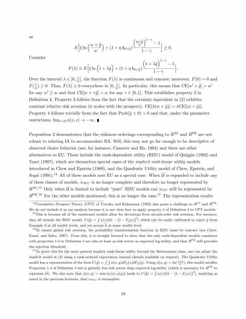
Proposition 2 demonstrates that the riskiness orderings corresponding to RAS and RFH are not

robust to relaxing IA to accommodate BA. Still, this may not go far enough to be descriptive of

observed choice behavior (see, for instance, Camerer and Ho, 1994) and there are other

alternatives to EU. These include the rank-dependent utility (RDU) model of Quiggin (1982) and

Yaari (1987), which are themselves special cases of the implicit rank-linear utility models

introduced in Chew and Epstein (1989), and the Quadratic Utility model of Chew, Epstein, and

Segal (1991).14 All of these models nest EU as a special case. When U is expanded to include any

of these classes of models, <WU is no longer complete and therefore no longer represented by

RAS.15 Only when U is limited to include “pure” RDU models can <UU still be represented by

RFH.16 For the other models mentioned, this is no longer the case.17 The representation results

14Cumulative Prospect Theory (CPT) of Tversky and Kahneman (1992) also poses a challenge to RAS and RFH.

We do not include it in our analysis because it is not clear how to apply property 4 of Definition 4 to CPT models.15This is because all of the mentioned models allow for deviations from second-order risk aversion. For instance,

they all include the RDU model, U(g) =∫u(x)d[1 −

(1 − Fg(x)

)2] which can be easily calibrated to reject g from

Example 3 at all wealth levels, and yet accept h at some wealth level.16To ensure global risk aversion, the probability transformation function in RDU must be concave (see Chew,

Karni, and Safra, 1987). From this, it is straight forward to show that the only rank-dependent models consistent

with properties 1-4 in Definition 4 are also at least as risk averse as expected log-utility, and thus RFH still provides

the rejection threshold.17To prove this for the more general implicit rank-linear utility beyond the Betweenness class, one can adopt the

implicit model in (2) using a rank-ordered expectation instead (details available on request). The Quadratic Utility

model has a representation of the form U(g) =∫ ∫

φ(x, y)dFg(x)dFg(y). Using φ(x, y) = ln(x+y2

), this model satisfies

Properties 1-4 of Definition 4 but is globally less risk averse than expected log-utility (which is necessary for RFH to

represent U). We also note that φ(x, y) = min(u(x), u(y)

)leads to U(g) =

∫u(x)d[1 −

(1 − Fg(x)

)2], implying as

noted in the previous footnote, that <WU is incomplete.

18

for RAS and RFH fail for an even larger class of well-behaved though as yet unaxiomatized models

that nest EU.18 The preceding discussion suggests that Theorem 1 may be better viewed as a

knife-edge result rather than reflective of universal tastes.

5 Quibbles III: Normative Desirability

5.1 Scale issues

Consider the position of a regulator intending to limit the risk undertaken by banks and other

institutions that are deemed “too big to fail”. A typical risk-management approach may specify

that the institution has to maintain a nominal amount of safe and liquid capital commensurate

with the riskiness of profit opportunity (e.g., a loan or a zero-cost derivative position).

Traditionally, such policies have been based on measures such as the standard deviation, or

sometimes the value at risk, of g. Here, we argue that using RAS and RFH to specify risk-based

capital instead may yield less satisfactory results. Suppose that riskiness was measured only using

RAS or RFH and thus capital requirements were set using only a monotonic transformation of one

or both of these measures. Then the following proposition raises concerns.

Proposition 3.

1. Given any ε ∈ (0,∞), let ∆ε be the set of all finite-outcome gambles in G whose support is a

strict subset of (−ε, ε). Then RAS(∆ε) = RFH(∆ε) = (0,∞).

2. Let δ0 correspond to the sure profit of zero. Then for any g ∈ G and α ∈ [1, 0),

RAS(g) = RAS(αg ⊕ (1− α)δ0) and RFH(g) = RFH(αg ⊕ (1− α)δ0).

Proof. To prove the first part, consider any binary gamble in ∆ε that is symmetric about its

mean, µ. Denoting the standard deviation as σ, for the low outcome to be negative it must be

that σ > µ. It is straight forward to show that RFH = σ2−µ22µ and RAS = σ

x where x solves

ln(

cosh(x))

= µσx. In both cases, as µ

σ tends to zero, R tends to infinity; likewise, as µσ tends to

one, R tends to zero.

18A simple example is the following: Let CEu[w+g] correspond to the certainty equivalent of w+g from an expected

utility model with utility function u. Then for any β ∈ (0, 1), the certainty equivalent CEu1 [w+g]βCEu2 [w+g]1−β will

violate IA unless u1 and u2 are affine equivalent (expected utility forms a strict subset of this class of models). Setting

u1(x) = lnx and u2(x) =√x leads to a certainty equivalent that is compatible with properties 1-4 in Definition 4 and

less risk-averse than expected log-utility (inconsistent with RFH). Setting, instead, u2(x) = −e−ax and, say, β = 12

can lead to inconsistency with RAS. If U contains all preferences in this class satisfying properties 1-4 in Definition

4, it is straight forward to show that a result identical to Proposition 2 obtains.

19

To prove part ii, consider

E[

exp(− αg ⊕ (1− α)δ0

RAS(g)

)]= αE

[exp

(− g

RAS(g)

)]+(1−α)E

[exp

( 0

RAS(g)

)]= α+(1−α) = 1,

where the last equality follows from the fact that RAS(g) solves E[

exp( gRAS(g)

)]= 1. The

calculation demonstrates that RAS(g) solves E[

exp(αg⊕(1−α)δ0

RAS(g)

)]= 1. Thus

RAS(g) = RAS(αg ⊕ (1− α)δ0). An analogous argument, also documented in Foster and Hart

(2009), establishes the result for RFH(g).

Proposition 3.1 establishes that within the set of (arbitrarily) small gambles, RAS and RFH take

on every conceivable value. In other words, the riskiness measures RAS and RFH do not convey

the scale of the outcomes in the sense that a report of RAS(g) says nothing about whether

differences in potential outcomes of g can be sizable. Relatedly, Proposition 3.2 establishes that

RAS and RFH do not convey the scale of the likelihood of non-zero profits. The bottom line is that

these measures necessitate a potentially unintuitive or descriptively inaccurate link between the

ranking of small or low-probability profits and those of profit opportunities with moderate or

large variance. In the context of risk-based capital regulation, Proposition 3.1 suggests that a risk

involving arbitrarily small gains and losses will require as much capital as one that has arbitrarily

large gains and losses. Likewise, according to Proposition 3.2, a risk involving only a tiny

likelihood of substantial loss will require as much capital as one with a high likelihood of

substantial loss. In the case of RFH, Foster and Hart (2009) recognize property (ii) of Proposition

3 as “dilution” and rationalize the invariance of RFH to dilution by noting that an infinitely

repeated sequence of a gamble leads to a non-zero probability of bankruptcy if and only if its

diluted counterpart does as well. We revisit this inherently dynamic alternative rationale for

measuring risk in Section 5.3.

The reason for the result in Proposition 3, partly illustrated in its proof, is that RAS and RFH

diverge as E[g] tends to zero. Even though riskiness intuitively declines as either the magnitude

of possible outcomes shrinks or the likelihood of non-zero profit shrinks, the mean of the gamble

simultaneously shrinks, potentially keeping RAS and RFH constant or even causing them to

increase — depending on the rate at which the mean decreases. Every measure of riskiness that is

FSD- and SSD-monotonic necessarily confounds “risk” and “reward”. What is special about RAS

and RFH is that, for any gamble with bounded payoffs, they diverge as Var[g]2E[g] in the limit

E[g]→ 0. In that sense, these may be better viewed as measures of a risk’s performance (similar

to the inverse Sharpe Ratio) than an appropriate dollar-denominated risk premium.19 Based on

19Both Aumann and Serrano (2008) and Foster and Hart (2009) argue that measures of riskiness should be FSD-

monotonic. We do not take issue with that statement. The dollar “risk-premium”, generated by subtracting from w

20

the above analysis of the small mean behavior of RAS and RFH, one may hope to disentangle the

risk from the reward by considering an alternative riskiness measure of the form f(E[g], R(g))

where f is increasing in both its arguments, homogeneous of degree one, and finite as E[g]→ 0.

For instance,√

2E[g]R(g) is finite whenever the outcomes of g are bounded and scales

proportionately with g. In particular, as E[g] tends to zero while holding variance constant, this

measure converges to the standard deviation of g. However,√

2E[g]RAS(g) and√

2E[g]RFH(g)

are not monotonic in E[g], thus undermining one of the advantages of these measures over

variance (and other coherent measures).20 This problem is pervasive as demonstrated below.

Proposition 4. Consider any f : R× R 7→ R+ that is increasing in both arguments, is

homogeneous of degree one, and such that for any constant a > 0, limx→0 f(x, ax) <∞. Then, for

either R(g) = RAS(g) or R(g) = RFH(g), f(E[g], R(g)) is increasing in µ for some g = µ+ ε ∈ G.

Proof. By the homogeneity of f , define f(µ,R) = µf(1, Rµ ) ≡ µϕ(Rµ ). The limit condition

becomes limµ→0 µϕ( aµ2

) <∞, which means that limz→∞ ϕ(z) ∼ b√z + o(

√z), where b is a

constant.21 Consider now that R = R(µ). Taking the derivative,

d

dµµϕ(R(µ)

µ

)= ϕ+

( ddµ

R(µ)− R

µ

)ϕ′. (3)

For the adjusted measure to be decreasing in µ, it must be that ϕ ≤(− d

dµ R(µ) + Rµ

)ϕ′. Write

g = µ+ ε for some zero-mean random variable ε. For the Foster and Hart (2009) measure, we

calculate that

d

dµRFH(g) =

E[

RR+g

]E[

gR+g

] .For g = ex(eye − 1) considered in Proposition 1, with RFH(g) = ex, the derivative of RFH(g)

reduces tod

dµRFH(g) =

E[e−ye]

1− E[e−ye].

In the case of the binary e discussed in the proof of Proposition 1, recall that we are free to

choose E[e−ye] ∈ (1,∞), thus for any µ and R fixed, we can choose ddµ R

FH(g) ∈ (−∞,−1).

the certainty equivalent of w+ g using any one of the models in UH , can also be viewed as a measure of riskiness. It is

FSD- and SSD-monotonic in G, and does not exhibit the scale conundrums of RAS and RFH. The main shortcoming

of the dollar risk-premium just described is that it is not“universal”. The arguments in Section 4 suggest that the

universality advantages of RAS and RFH are limited.20Consider, for example, the binary gamble g that with probability p > 0 yields µ+ σ

√1−pp

and otherwise yields

µ − σ√

p1−p , where σ, µ > 0. For such a gamble to be admissible, it must be that µ < σ

√p

1−p . It is easy to check

that for p = 0.75 and σ = 1 the measures√

2µRAS(g) and√

2µRAS(g) have inverted-U shapes for µ ∈ [0.4, 0.9].21o(√z) denotes a term with the property that limz→∞ z

− 12 o(√z)→ 0.

21

Imposing this result on Equation (3), a necessary condition for f(E[g], RFH(g)) to decrease with µ

is that ϕ ≤(1 + R

µ

)ϕ′. Applying this inequality to the asymptotic condition for ϕ and setting

z = Rµ , yields b

√z + o(

√z) ≤ (1 + z)

(b

2√z

+ o( 1√z)), which is violated for z sufficiently large.

For the Aumann and Serrano (2008) measure, we calculate that

d

dµRAS(g) =

1

E[gRe− gR

] .For g = µ+ σe, as considered in Proposition 1, the denominator can taken on any value in

(−∞, 0), meaning that for any fixed R and µ we can find a corresponding g such that ddµ R

AS

takes any desired value in (−∞, 0). Using this result in Equation (3), a necessary condition for

f(E[g], RAS(g)) to decrease with µ is that ϕ ≤ Rµϕ′. Applying this inequality to the asymptotic

condition for ϕ and setting z = Rµ , yields b

√z + o(

√z) ≤ z

(b

2√z

+ o( 1√z)

)), which is also violated

for z sufficiently large.

In contrast with RAS and RFH, both of which are not separable in the mean of the gamble

evaluated, conventional measures of riskiness like variance, value-at-risk, and/or coherent

measures a la Artzner, Delbaen, Eber, and Heath (1999) convey, or can be adjusted to reflect, a

sense of the magnitude of risk independent of the mean. For such mean-adjusted measures, large

variance gambles engender greater risks because they allow for a greater likelihood of large

differences in outcomes. Proposition 3 indicates that these statements are not true of RAS and

RFH, while Proposition 4 implies that any attempt to mean-adjust RAS and RFH would generally

result in measures that are not FSD-monotonic.

Returning once more to regulating risk-based capital, suppose that the capital requirements are

determined using some function of RAS and RFH and the mean of the profit opportunity.

Proposition 4 tells us that such capital requirements would feature the perverse implication that,

at least in some cases, a positive shift in profit across all possible outcomes will lead to higher

capital requirements. One way to avoid this would be to include additional information (other

than the mean, RAS and RFH) about the distribution of profits — in other words, employ

additional riskiness measures in the exercise. This, however, undermines any “special” status

alloted to RAS or RFH and calls into question the need for them in the first place. In summary,

propositions 3 and 4 raise concerns about the use of RAS and RFH as tools in the measurement

and management of risk.

22

5.2 Illiquid markets

The measures of riskiness RAS and RFH apply only to “gambles” that have positive mean and a

non-zero probability of a negative outcome. In Section 2 we argue that this is suitable for a

setting in which any risky position can be liquidated and the proceeds invested in some risk-free

asset so that a sure outcome is always available. In many cases, reality presents a sufficiently

good approximation to this situation that there is no reason to take issue with such an

assumption. There are, however, important settings in which this approximation materially fails.

Difficulties arise, for instance, if one attempts to evaluate RAS or RFH for a prospect or current

investment position that is non-tradeable or highly illiquid. Consider any one of the various

financial institutions that were heavily invested in complicated structured products during the

Winter of 2008-2009. A market price might not have existed even if it might have been possible to

assign a probability distribution to the value of the institution’s portfolio. At a time when risk

measurement was most needed and while one could still calculate the variance or value-at-risk of

such a portfolio, one might not have been be able to calculate its Aumann and Serrano (2008) or

Foster and Hart (2009) measures.

Another example of a situation that is perhaps more pervasive is that of risk assessment at the

non-institutional level. A small enterprise (or family business) may have need for risk assessment

that cuts across preferences, underscoring the attractiveness of measures that are “universal”.

Suppose that such an entity was capable of calculating the distribution of possible future

outcomes for each of several financial and real investment strategies.22 While standard utility

theory or standard approaches to risk measurement would at this point produce a ranking of

options, this would not be the case if one attempts to calculate RAS or RFH because of the thorny

issue of evaluating the “wealth” of the enterprise, which itself can and typically does carry

significant uncertainty (e.g., real estate valuation, the value of human capital, etc.). In summary,

leaving aside the arguments put forth in Section 4, the additional requirement of risk-free wealth

as a reference point for assessing RAS and RFH is far from innocuous and limits their consistent

application across a satisfactory range of situations.23

22This is a necessary assumption for any decision making approach under risk.23The Cumulative Prospect Theory of Tversky and Kahneman (1992) also features a reference point that is crucial

in determining the merits of various decisions. An important difference is that Prospect Theory is motivated by

psychological biases observed in experiments and generally limits itself to contexts where a status quo is obvious,

without making claims to being broadly operationalizable.

23

5.3 Intertemporal rationale

Foster and Hart (2009) provide an additional rationale for the use of their measure, distinct from

what we have discussed in the Introduction and expounded in Hart (2011). Specifically, RFH(·)can be viewed as the unique solution to the following problem. Suppose a decision maker with

initial wealth w1 faces a sequence of unknown independent profit opportunities, (g1, g2, . . .), such

that gt ∈ G for all t. The decision maker only knows the distribution of gt at date t and at that

point must decide whether to accept or reject it. A “simple rule” is a function, Q : G 7→ R+ that

is homogeneous of degree one. A simple rule strategy will only accept a date-t profit opportunity

from the sequence if Q(gt) ≤ wt. The task is to find the minimal simple rule that guarantees

solvency. Foster and Hart (2009) establish that RFH(g) is the solution to that task. This, too, is

an elegant formulation justifying the operational use of RFH(·). For instance, a bank that is to

remain solvent should ensure that the present value of its portfolio, w, is greater than or equal to

RFH(w) or raise enough capital for this to be the case.

One problem with this rationalization is that it is not obviously linked to an inter-temporal profit

function that a bank or its regulator might seek to optimize. In other words, this formulation is

not justified by more general considerations of inter-temporal optimization with solvency

constraints. Instead, it relies on the stylized assumption that the decision maker does not make

use at date t of information about future distributions either because (s)he does not want to or

because the information is not available.24 The following two examples demonstrate that, relative

to the simple strategy specified via RFH(·), employing information about future distributions can

lead to an alternative strategy that delivers higher utility while guaranteeing solvency.

To place the following into context, note that RFH(g) is the smallest wealth, w, at which an

expected log utility maximizer is willing to choose w + g over w.

Example 4. Suppose a decision maker knows that each gt in the sequence of of gambles to be

faced is an independently distributed binary random variable paying 110 with probability 12 and

−100 otherwise. We calculate that RFH(gt) = 1100. This means that if w1 = 1070 then, when

restricted to simple rules, the entire sequence will be rejected. Consider, however, the “less simple

rule” for which g1 is accepted at w1 ≥ 1070, g2 is accepted only if the outcome of g1 is high, and

gt is rejected for all t > 2. The alternative strategy is solvent because the maximum loss is 100 —

this is because no risk is taken after t > 2. Moreover, a straight-forward calculation demonstrates

24Foster and Hart (2009) concede that their framework is not Bayesian. Another critical assumption is that the

acceptance rule is homogeneous of degree one. Foster and Hart (2009) show that if one allows for more general

strategies, then to avoid bankruptcy the simple acceptance/rejection criterion defined by RFH(·) only matters when

wealth is sufficiently small.

24

that an expected log-utility maximizer would receive a higher EU by accepting this strategy than

by rejecting the entire sequence and keeping w1 = 1070 (as directed by the simple rule based on

constraints RFH). It is easy to show that there are strategies, contingent on the path of outcomes,

that deliver even higher utility. The bottom line is that such strategies dominate the simple rule

and can be employed because one can make use of information about the distribution of future

gambles.

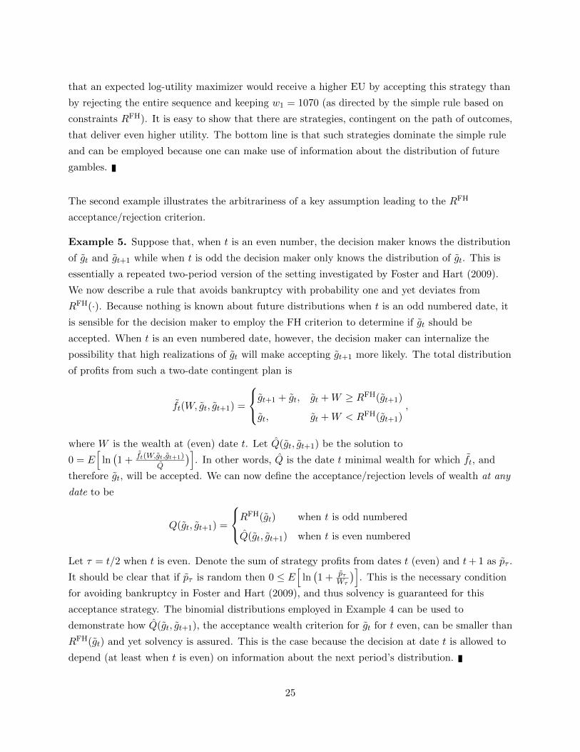
The second example illustrates the arbitrariness of a key assumption leading to the RFH

acceptance/rejection criterion.

Example 5. Suppose that, when t is an even number, the decision maker knows the distribution

of gt and gt+1 while when t is odd the decision maker only knows the distribution of gt. This is

essentially a repeated two-period version of the setting investigated by Foster and Hart (2009).

We now describe a rule that avoids bankruptcy with probability one and yet deviates from

RFH(·). Because nothing is known about future distributions when t is an odd numbered date, it

is sensible for the decision maker to employ the FH criterion to determine if gt should be

accepted. When t is an even numbered date, however, the decision maker can internalize the

possibility that high realizations of gt will make accepting gt+1 more likely. The total distribution

of profits from such a two-date contingent plan is

ft(W, gt, gt+1) =

gt+1 + gt, gt +W ≥ RFH(gt+1)

gt, gt +W < RFH(gt+1),

where W is the wealth at (even) date t. Let Q(gt, gt+1) be the solution to

0 = E[

ln(1 + ft(W,gt,gt+1)

Q

)]. In other words, Q is the date t minimal wealth for which ft, and

therefore gt, will be accepted. We can now define the acceptance/rejection levels of wealth at any

date to be

Q(gt, gt+1) =

RFH(gt) when t is odd numbered

Q(gt, gt+1) when t is even numbered

Let τ = t/2 when t is even. Denote the sum of strategy profits from dates t (even) and t+ 1 as pτ .

It should be clear that if pτ is random then 0 ≤ E[

ln(1 + pτ

Wτ

)]. This is the necessary condition

for avoiding bankruptcy in Foster and Hart (2009), and thus solvency is guaranteed for this

acceptance strategy. The binomial distributions employed in Example 4 can be used to

demonstrate how Q(gt, gt+1), the acceptance wealth criterion for gt for t even, can be smaller than

RFH(gt) and yet solvency is assured. This is the case because the decision at date t is allowed to

depend (at least when t is even) on information about the next period’s distribution.

25

While individuals and institutions may have little information about their investment

opportunities in the very distant future, the notion that this is true at horizons relevant for risk

management/measurement, (e.g., quarterly) seems far-fetched. The preceding examples establish

that, when it is available, ignoring information about future opportunities — which is a

fundamental assumption in the development of RFH(·) as a riskiness measure — can lead to

inefficient outcomes. To the extent that in most realistic applications there will be some

information about future distributions, RFH is generally associated with solvent strategies that

are suboptimal.

6 Conclusions

This paper takes a critical look at the two influential measures of riskiness of Aumann and

Serrano (2008) and Foster and Hart (2009). We raise several fundamental concerns having to do

with their operationalizability as well as claims of objectivity and universality relative to all

decision makers with Expected Utility preferences in the set of “unobjectionable preferences”, UH ,

characterized by Hart (2011). By examining mean-riskiness efficient portfolios and the Pareto

frontier for UH , we demonstrate that one can find a mean-riskiness efficient portfolio that strictly

dominates some point on the Pareto frontier (in the sense of both mean and riskiness). That is,

no investor will hold this portfolio even though it strictly dominates some investor’s portfolio.

Restricting ourselves to preferences in UH , we provide an example in which the optimal portfolio

of one investor strictly dominates the optimal portfolio of another globally less risk averse

investor. We also demonstrate that the preference represented by any differentiable ranking of

gambles trading off the mean against the riskiness results violate the Independence Axiom of

Expected Utility and is therefore not a member of UH . These findings suggest an inconsistency

between the operationalization of RAS or RFH and the idea that they characterize a notion of

riskiness on which all investors with unobjectionable preferences can agree. Thus attempts to

replace mean variance analysis (or similar approaches) with mean-riskiness analysis undermine

the very assumptions that endow the riskiness measures with a sense of objectivity.

At the same time, we follow the suggestion in Hart (2011) to consider more general settings that

include non-expected-utility models in trying to capture universal notions of “more risky”. As it

turns out, even though both RAS and RFH satisfy the Betweenness Axiom which weakens the

Independence Axiom of Expected Utility, they are not universal with respect to the set of

betweenness-conforming preferences that generalizes UH . Moreover, we show that upon such

generalizations, no measures featuring the desirable attributes mentioned in Hart (2011) apply

uniformly across preferences or wealth levels. This suggests that Hart’s (2011) universality results

26

are knife-edge.

We also note that there are risk management, regulatory capital requirement, and decision

making settings for which reliance on RAS and RFH could be problematic. For instance, a

prospect involving only insignificant gains and losses might be deemed riskier than one allowing

for arbitrarily large gains and losses. Likewise, a profit opportunity involving a high probability of

substantial loss can be assessed to be as risky as one with only a tiny probability of substantial

loss. Additionally, we note that RAS and RFH are only applicable in situations where a prospect’s

present value is accurately identifiable and where a risk-free alternative is available. This limits

their application to settings involving only highly liquid investment opportunities. Finally, we

show that the minimal solvency interpretation of RFH put forward in Foster and Hart (2009) is

not applicable in situations where there is even a minimal amount of information about the

distributions of future profit opportunities.

The derivation of the Aumann and Serrano (2008) and Foster and Hart (2009) measures of

riskiness is elegant and economically motivated. Rather than to discourage their application, our

goal is to point out that justifications for their use on the basis of their universality, objectivity,

normative qualities, or scope of application may have severe limitations. At the same time,

together with other measures of riskiness in the literature, such as the Sharpe Ratio or Value at

Risk, the RAS and RFH measures may well contribute to a robust approach to comprehensive risk

management and risk-return trade-off analysis.

References

Allais, M., 1953, “Le comportement de l’homme rationnel devant le risque: critique des postulats

et axiomes de l’ecole Americaine,” Econometrica, 21, 503–546.

Artzner, P., F. Delbaen, J.-M. Eber, and D. Heath, 1999, “Coherent Measures of Risk,”

Mathematical Finance, 9(3), 203–228.

Aumann, R. J., and R. Serrano, 2008, “An Economic Index of Riskiness,” Journal of Political

Economy, 116(5), 810–836.

Berk, J. B., 1997, “Necessary Conditions for the CAPM,” Journal of Economic Theory, 73(1),

245–257.

Camerer, C. F., and T.-H. Ho, 1994, “Violations of the Betweenness Axiom and Nonlinearity in

Probability,” Journal of Risk and Uncertainty, 8(2), 167–96.

27

Chew, S. H., 1983, “A Generalization of the Quasilinear Mean with Applications to the

Measurement of Income Inequality and Decision Theory Resolving the Allais Paradox,”

Econometrica, 51(4), 1065–92.

, 1989, “Axiomatic Utility Theories with the Betweenness Property,” Annals of Operations

Research, 19, 273–298.

Chew, S. H., and L. G. Epstein, 1989, “A unifying approach to axiomatic non-expected utility

theories,” Journal of Economic Theory, 49(2), 207 – 240.

Chew, S. H., L. G. Epstein, and U. Segal, 1991, “Mixture Symmetry and Quadratic Utility,”

Econometrica, 59, 139–63.

Chew, S. H., E. Karni, and Z. Safra, 1987, “Risk Aversion in the Theory of Expected Utility with

Rank Dependent Probabilities,” Journal of Economic Theory, 42, 370–381.

Chew, S. H., and M. H. Mao, 1995, “A Schur Concave Characterization of Risk Aversion for

Non-expected Utility Preferences,” Journal of Economic Theory, 67, 402–435.

Dekel, E., 1986, “An Axiomatic Characterization of Preferences Under Uncertainty: Weakening

the Independence Axiom,” Journal of Economic Theory, 40, 304–318.

Dybvig, P. H., and Y. Wang, 2012, “Increases in risk aversion and the distribution of portfolio

payoffs,” Journal of Economic Theory, 147(3), 1222–1246.

Epstein, L. G., and S. E. Zin, 1990, “’First-order’ risk aversion and the equity premium puzzle,”

Journal of Monetary Economics, 26(3), 387–407.

Foster, D. P., and S. Hart, 2009, “An Operational Measure of Riskiness,” Journal of Political

Economy, 117(5), 785–814.

Gul, F., 1991, “A Theory of Disappointment Aversion,” Econometrica, 59(3), 667–86.

Hart, S., 2011, “Risk by Acceptance and Rejection,” Journal of Political Economy, 119(4),

617–638.

Hellmann, T., and F. Riedel, 2013, “The Foster-Hart Measure of Riskiness for General Gambles,”

Social Science Research Network Working Paper Series.

Herstein, I. N., and J. Milnor, 1953, “An Axiomatic Approoach to Measureable Utility,”

Econometrica, 21, 291–297.

Ingersoll, J. E., 1987, Theory of financial decision making, vol. 3. Rowman & Littlefield.

28

Machina, M. J., 1982, “Expected Utility Analysis without the Independence Axiom,”

Econometrica, 50(2), 277–323.

Quiggin, J., 1982, “A Note on the Existence of a Competitive Optimal Output,” The Economic

Record, 58(161), 174–76.

Rabin, M., 2000, “Risk Aversion and Expected-Utility Theory: A Calibration Theorem,”

Econometrica, 68(5), 1281–1292.

Schulze, K., 2014, “Existence and computation of the AumannSerrano index of riskiness and its

extension,” Journal of Mathematical Economics, 50(0), 219 – 224.

Segal, U., and A. Spivak, 1990, “First order versus second order risk aversion,” Journal of

Economic Theory, 51(1), 111–125.

Starmer, C., 2000, “Developments in Non-expected Utility Theory: The Hunt for a Descriptive

Theory of Choice under Risk,” Journal of Economic Literature, 38(2), 332–382.

Tversky, A., and D. Kahneman, 1992, “ Advances in Prospect Theory: Cumulative

Representation of Uncertainty,” Journal of Risk and Uncertainty, 5(4), 297–323.

Yaari, M. E., 1987, “The Dual Theory of Choice under Risk,” Econometrica, 55, 95–115.

29