A Crisis of Missed Opportunities?Foreclosure Costs and Mortgage Modification During

the Great Recession

Stuart Gabriel∗

University of California, Los Angeles

Matteo Iacoviello†

The Federal Reserve Board

Chandler Lutz‡

Copenhagen Business School

June 25, 2016

Abstract

This paper investigates the housing and broader economic effects of the 2000s crisis- period California Foreclosure Prevention Laws (CFPLs). The CFPLs encouraged lenders to modify mortgage loans by increasing the required time and pecuniary costs of foreclo- sure. Using the Synthetic Control Methodology, we find that the CFPLs prevented 335,000 California foreclosures, equivalent to a 30% reduction during the treatment period. These effects did not reverse after the conclusion of the policy, implying that the CFPLs were not a stopgap measure that simply delayed foreclosures until a later date. Our analysis also shows that the CFPLs increased house prices by 5 percent and in doing so created $250 billion of housing wealth. Findings further indicate that these gains in housing wealth did not translate into increased durable consumption as measured by auto sales. Disaggregated county and zip-code level estimates reveal that the CFPL house price increases were markedly higher in the hard hit areas of Southern California. Altogether, results suggest that the CFPLs were substantially more effective than the US Government’s HAMP Program in mitigating foreclosures and stabilizing the housing markets.

JEL Classification: E52, E58, R20, R30 ;

Keywords: Mortgage Modification, Foreclosure Costs, Housing Crisis

∗stuart.gabriel@anderson.ucla.edu. Gabriel acknowledges funding from the UCLA Gilbert Program inReal Estate, Finance, and Urban Economics.†matteo.iacoviello@frb.gov‡cl.eco@cbs.dk

1 Introduction

In the wake of the 2000s boom-period run-up in house prices, California in 2005 accounted

for one-quarter of US housing wealth.1 But as the 2006 boom turned to the 2008 bust,

house prices in the state fell by 30 percent and 1 million California borrowers lost their

homes to foreclosure.2 In an effort to contain mounting home foreclosures both in Califor-

nia and beyond, the Federal Government enacted Home Affordable Modification Program

(HAMP), which sought to modify distressed mortgages by offering financial incentives to

both homeowners and lenders.3 Yet, as shown by Agarwal et al. (2012), HAMP had little

economic impact as many mortgage lenders lacked the infrastructure to modify loans on

a large scale.4 At the epicenter of the housing bust, the State of California pursued an

alternative policy approach to aid distressed borrowers and limit substantial foreclosures.

Rather than offering financial incentives to modify loans as in HAMP, the California poli-

cies instead imposed foreclosure moratoriums and incremental pecuniary costs on lenders

to encourage their widespread adoption of mortgage modification programs. Thus in the

California policy response, distressed borrowers received policy treatment even in the event

of inaction by their lenders.5 Unlike HAMP, there has been little attention paid to and no

prior evaluation of alternative policy efforts that used increased foreclosure costs to stem the

housing and foreclosure crisis. In this paper, we undertake such an evaluation and use Cali-

fornia as a laboratory to measure the housing and broader economic effects of the California

Foreclosure Prevention Laws (CFPLs).

California is an non-judicial foreclosure state. Prior to the enactment of the CFPLs, the

state only required a lender initiating a foreclosure to deliver a notice of default (NOD; fore-

closure start) to the borrower by mail. A 90-day waiting period then commenced before the

lender could issue a notice of sale (NOS) for the property. In July of 2008 and in the midst of

1Number of housing units by state from table S1101 of the 2005 American Community Survey. State-level house prices are from Zillow in 2005.

2California house prices from the FRED economic database. The number of California foreclosures isfrom Zillow.

3The Federal Government also implemented other housing policy during the crisis. These programs arediscussed below in section 2.

4Specifically, Agarwal et al. (2012) find HAMP reached just a third of the targeted 3-4 million house-holds.

5Inaction by both lenders and borrowers was a constraint in many mortgage modification programs.Section 2 discusses these issues in more detail.

1

a severe housing crisis, the state passed the first of the CFPLs, Senate Bill 1137 (SB-1137).6

This bill, which immediately went into effect, prohibited mortgage lenders and servicers

(henceforth, lenders) from issuing a NOD until 30 days after informing the homeowner of

potential foreclosure alternatives either by telephone or in person.7 The homeowner then

had the right within 14 days of first contact to schedule a second telephonic meeting with the

lender to discuss foreclosure alternatives. SB-1137 additionally mandated that agents who

obtained a vacant residential property through home foreclosure maintain the property or

face fines of up to $1000 per day, further increasing lender out-of-pocket foreclosure costs. In

the second CFPL wave, California passed the California Foreclosure Prevention Act (CFPA)

in early 2009. The CFPA prohibited mortgage lenders from sending borrowers a NOS for

an additional 90 days after the NOD unless the lender had implemented a comprehensive

mortgage modification program. The adequacy of the mortgage modification programs was

determined by the State of California based on debt-to-income targets and potential inter-

est rate or principal payment reductions.8 Therefore, like SB-1137, the CFPA extended the

duration and pecuniary costs of foreclosure in an effort to encourage widespread mortgage

modification and limit the ongoing and extensive mortgage default crisis.

The CFPLs were unique in their scope and intervention. Further, they were implemented

at a moment when prices in many California housing markets were spiraling downward.

As such, these policies provide a rare and important opportunity to use cross-sectional

variation to assess the housing and related economic effects of crisis-period law which sought

to encourage widespread mortgage modification. Using the Synthetic Control Methodology

(SCM) and data at various levels of geography, we find that the CFPLs reduced (Real Estate

Owned (REO)) foreclosures by 30 percent and hence prevented 335,000 California borrowers

from losing their homes. The CFPLs also mitigated prime and subprime foreclosure starts

and ameliorated housing distress.

Our most conservative estimate of the relative gain in California house prices due to the

CFPLs is 5 percent – equivalent to a $250 billion increase in housing wealth.9 Our median

6ftp://www.leginfo.ca.gov/pub/07-08/bill/sen/sb 1101-1150/sb 1137 bill 20080708 chaptered.html7If lenders could not reach homeowners, they had to undertake “due diligence” in their attempts to

contact the homeowner. See section 2 for more details.8See section 2 for more details.9According to table S1101 of the 2007 1-Year ACS Community Survey, there were 12,200,672 homes

in California is 2007. The median house price in 2008M06 according to Zillow was $413,000. Thus,$413,200*12,200,672*0.0479 ≈ $250 billion.

2

estimate of the house price appreciation due to the CFPLs, found using highly disaggregated

zip code level data, is 9.5 percent. These effects were largely concentrated in the hard-hit

areas of Southern California. Indeed, using zip code level data, we find that the CFPLs

caused a 15.8 percent relative house price increase in the Southern California Coastal and

Inland Region.

To put the CFPL house price gains into perspective, note that the effective US Govern-

ment fiscal stimulus during the crisis, through the American Recovery and Reinvestment

Act of 2009 (ARRA) and social transfers, totaled $114 billion.10 The magnitude of the

housing stimulus created by the CFPLs ($250 billion using our most conservative estimate)

was thus 220 percent of the effective US Government package. This implies that our CFPL

estimates are large in magnitude, economically meaningful, and highlight how the CFPLs

ameliorated the decline in California housing markets during the policy period.

Despite the aforementioned bolstering of housing markets, the broader economic effects

of the CFPLs were limited as we find no evidence of an increase in durable consumption as

measured through auto sales. These findings are consistent across California and in areas

where the CFPLs housing impacts were highly beneficial. For example, in Los Angeles

County, the CFPLs increased house prices by 15 percent and created $188 billion of housing

wealth. This rise in house prices was evidenced in 70 percent of Los Angeles zip codes. Yet

we find no increase in Los Angeles County auto sales per capita due to the introduction of

the CFPLs, suggesting a muted impact of the CFPLs beyond the housing sector.

A priori, the housing market effects of the CFPLs were uncertain. Larry Summers,

the Director of the National Economic Council during the crisis, noted that the Federal

Government elected not to increase foreclosure durations as any such increase would sim-

ply delay foreclosures until a later date.11 This was the prevailing view among leading US

policymakers during the crisis.12 Further, other government loan modification programs

enacted during the crisis were largely unsuccessful (Agarwal et al. (2012)). On the other

10Oh and Reis (2012) find that the increase in discretionary transfers from 2007-2009 was $96 billion (seealso Kaplan and Violante (2014)), while Cogan and Taylor (2013) find that only $18 billion of ARRA stimuluswas spent for federal purchases. The remainder of ARRA funds were granted to states who subsequentlyreduced their borrowing. The total effective discretionary fiscal increase from 2007-2009 was $114 billion.

11“Lawrence Summers on ‘House of Debt’ ”. Financial Times. June 6, 2014. Note that Summers didnot discuss the potential effects of programs that increased both costs and durations.

12See, for example, “Geithner Calls Foreclosure Moratorium ‘Very Damaging’ ”. Bloomberg News. Oc-tober 10, 2010.

3

hand, prior academic research provides a basis through which the CFPLs may affect housing

markets. First, Pence (2006) notes that judicial foreclosure laws – laws that mandate that

lenders must process foreclosures in state courts – increase both the costs and duration of

the foreclosure process. Building on this observation, Mian et al. (2015) find that states

with a judicial foreclosure requirement experienced markedly lower rates of foreclosure and

relatively higher house prices during the 2000s housing crisis.13 The economic justification

for these house price gains in areas with with lower foreclosures is based on foreclosure exter-

nalities or theories of foreclosure induced fire sales. With regard to foreclosure externalities,

a large literature contends that a foreclosure negatively affects nearby house prices (the

so-called foreclosure spillover) by increasing housing supply (Anenberg and Kung (2014)) or

through a “disamenity” effect where distressed homeowners neglect maintenance on their

homes (Geradi et al (2015)).14 During a foreclosure induced fire sale, a downward house

price trend may reverse if the frequency with which houses become available for sale slows

(Mian et al. 2015).15 Hence by increasing the duration and cost of the foreclosure process,

the foregoing academic studies imply that CFPLs could have had a positive effect on housing

markets if these laws reduced the flow of homes that entered the foreclosure process.16 This

is what we find in our empirical work: The CFPLs lowered mortgage defaults and stemmed

the downturn in housing, suggesting that an increase in mandated foreclosure costs is effec-

tive in buttressing ailing housing markets. Further, in contrast to the views of Summers and

other leading policymakers, we find no evidence that policy effects reversed in later periods,

meaning that the CFPLs did prolong the crisis or simply delay foreclosures until a later

date.

The broader economic impacts of the CFPLs were also unclear ex ante as there has been

little agreement on the marginal propensity to consume (MPC) out of an increase in housing

wealth during a severe housing downturn. Tim Geithner (2014), the US Treasury Secretary

from 2009-2013, contended that the MPC out of an increase in housing wealth during the

crisis would have been a mere 0.01 or 0.02. This line of thinking postulates that households

13Goodman and Smith (2010) also find that states with lower default rates also placed higher pecuniaryand time foreclosure costs on lenders.

14See also Lambie-Hanson (2015) and the references therein.15See also Shleifer and Vishny (1992), Kiyotaki and Moore (1997), Krishnamurthy (2003, 2010), and

Lorenzoni (2008).16Bolton and Rosenthal (2002) See section 3 for a more detailed overview.

4

are unwilling or unable to increase consumption simply because the decline in the value of an

already highly depreciated, illiquid, hard-to-value asset is less steep. Specifically, increases in

housing wealth may effect consumption through a wealth channel or a collateral constraints

channel (e.g. equity withdrawal or refinancing). Yet note that the CFPLs lessened the

decline in house prices – house prices still fell during the treatment period, but the drop was

less steep due to the introduction of the CFPLs. Thus, the effects of the wealth channel are

likely to be small (see also Buiter (2008) and Sinai and Souleles (2013)), while in the case of

California the collateral channel is likely to be impotent as homeowners, especially those with

non-standard mortgages, may have had difficulty refinancing homes with already depressed

prices in the private market. Indeed, 60 percent of all mortgages originated in California

at the peak of the boom were interest only and thus unlikely candidates for subsequent

refinancing during the housing bust.17 In contrast, some recent academic research papers

suggest that the MPC out of housing wealth to ranges from 0.05 to 0.10.18 Our results

suggest that the CFPLs, while buttressing distressed housing markets, had little impact on

durable consumption measured through auto sales.

The remainder of this paper is organized as follows: Section 2 provides of a detailed

overview of the CFPLs; in section 3 we outline our main empirical hypotheses; the data and

econometric methodologies are described in sections 4 and 5; section 6 provides a preliminary

differences-in-differences analysis using just the Sand States that were highly exposed to the

housing boom–Arizona, California, Nevada, and Florida; the main Synthetic Control results

are in 7; and section 8 concludes.

2 The California Foreclosure Prevention Laws (CFPLs)

The State of California sought to mitigate the effects of the 2000s housing crisis first through

SB-1137 in July 2008 and then again with the passage of the CFPA in February 2009

(implemented in June 2009). The CFPLs aimed to provide mortgage lenders with incentives

to modify loans by increasing the pecuniary and time costs of foreclosure. The following

17Furhter, Mian et al. (2013) find that regions that suffered declines in housing wealthalso experienced tighter credit constraints during the Great Recession. In California, 60percent of all new mortgages originated in 2005 were non-standard interest only loansand anecdotal evidence suggests that these borrowers had trouble refinancing such loans:http://www.sfgate.com/news/article/High-interest-in-interest-only-home-loans-2634044.php

and http://www.nytimes.com/2009/09/09/business/09loans.html?pagewanted=all& r=0.18See Bostic et al. (2009) for an overview.

5

two sections discuss these laws in greater detail.

2.1 California Senate Bill 1137 (SB-1137)

California Senate Bill 1137 (SB-1137) was signed into law on July 8, 2008 and mandated that

mortgage lenders operating in California delay filing a notice of default (NOD), the first step

in the foreclosure process, until 30 days after contacting the homeowner with information on

foreclosure alternatives.19 Specifically, SB-1137 required the lender to contact the borrower

in person or over the telephone and notify the borrower of his right to schedule a meeting

with the lender to discuss foreclosure alternatives. The mortgagor then had the right to

schedule a meeting with the lender within 14 days of first contact. Then, after the initial

contact or attempted “due diligence”, the law required the lender to wait 30 days before filing

a NOD. Three attempts to contact the mortgagor over the telephone on different days and at

different times satisfied the law’s due diligence requirement. This due diligence requirement

likely created large institutional costs for lenders as many lacked the infrastructure to contact

borrowers by telephone on a large scale (Agarwal et al. (2012)). Further, the law required the

legal owner who took possession of a vacant residential property via foreclosure to maintain

it or face fines of up to $1000 per day.20

Prior to the enactment of SB-1137, existing law required only that the lender file a NOD

with the appropriate county recorder and then mail the NOD to the mortgage borrower. In

this letter, lenders were not obligated to provide any information on foreclosure alternatives.

The aim of SB-1137 was to alert struggling homeowners of foreclosure alternatives via

mortgage lenders. Indeed, the Bill’s chaptered text cites a Freddie Mac report that suggested

that 57 percent of late paying borrowers did not know that their lender may offer a foreclosure

alternative. Further, by increasing the pecuniary and time costs of foreclosure (for example,

by requiring maintenance of vacant foreclosed properties), the State of California sought to

change the net present value calculation of foreclosure versus mortgage modification.

19ftp://www.leginfo.ca.gov/pub/07-08/bill/sen/sb 1101-1150/sb 1137 bill 20080708 chaptered.html20Further, SB-1137 was only applicable for mortgages on owner-occupied homes originated between

January 1, 2003 and December 31, 2007.

6

2.2 The California Foreclosure Prevention Act (CFPA)

The CFPA was signed into law on February 20, 2009 and went into effect on June 15, 2009

for the period extending through January 1, 2011.21 The aim of the 2009 California Foreclo-

sure Prevention Act (CFPA) was to provide lenders incentives to implement comprehensive

mortgage modification programs during a period of housing crisis and widespread mortgage

failure. The CFPA prohibited lenders from handing defaulted homeowners a notice of sale

(NOS) for an additional 90 days after the initial NOD unless the lender enacted a mortgage

modification program meeting the requirements of CFPA. Note that as a non-judicial fore-

closure state, California already required a three month period between the NOD and the

NOS. Thus, under the CFPA, lenders that had not implemented loan modification programs

meeting the CFPA regulations were required to wait a total of six months between the NOD

and the NOS.22

Mortgage lenders who implemented an acceptable mortgage modification program were

exempted from the additional 90 day CFPA foreclosure moratorium. To obtain this exemp-

tion, a lender’s loan modification program was required to keep borrowers in their homes

when the anticipated recovery under the loan modification or workout exceeded the proceeds

from foreclosure on a net present value basis. Further, an adequate modification program

was required to achieve a housing-related debt to gross income ratio of 38 percent or less

on an aggregate basis and contain at least two of the following features: An interest rate

reduction over a fixed term for a minimum of five years; an extension of the loan amorti-

zation period up to 40 years from the original date of the loan; deferral of principal until

the maturity of the loan; a reduction in principal; compliance with a federal government

21Further, in March 2009, California established a timeline for the implementation of the CFPA andposted it online; on April 21, 2009 the CA government released a draft of the emergency regulations tointerested parties and accepted comments until May 6, 2009; On May 21, 2009, the emergency regulationsassociated with the CFPA were filed with the California Office of Administrative Law (OAL); and on June1, 2009, the OAL approved the emergency regulations and filed them with the Secretary of State.

22To be eligible for a mortgage modification under the CFPA a borrower must (1) live in the property; (2)be in default (foreclosure); (3) document an ability to pay the modified loan; (4) have obtained the mortgageunder consideration between January 1, 2003 to January 1, 2008; and (5) not have surrendered the propertyor engaged in a bankruptcy proceeding. The CFPA also required that mortgages under consideration formodification be the first lien on a property in California. All loans originated in California that meetthe above requirements were subject to the provisions of the CFPA. Loans where a servicing or poolingagreement prohibited modification are exempt from the CFPA. The State of California also outlined anumber of procedures related to the implementation of the CFPA. When a mortgage lender submitted anapplication for exemption under the CFPA, the State immediately issued a temporary order of exemptionfrom the CFPA foreclosure moratorium. Then, within 30 days, the lender received a final notification ofexemption or denial regarding the mortgage modification program.

7

mortgage program; or other factors that the state Commissioner deems appropriate. Note

that lenders participating in the federal government’s Home Affordable Modification Pro-

gram (HAMP) were considered to be in compliance with the CFPA and thus are exempt

from the extra 90 day foreclosure moratorium under the law.23

In total, 149 applications were submitted for exemptions from the CFPA foreclosure

moratorium. Of these 149 applications, 78.5 percent were accepted, 12 percent were denied,

and 10 percent of the applications were withdrawn. Hence, a non-trivial portion of the

submitted mortgage modification programs did not meet the CFPA standards. Of the

117 accepted applications, only 31 lenders obtained an exemption from the CFPA via the

US government’s HAMP program; indicating that the vast majority of lenders were not

participating in the federal program and thus that the CFPA may have provided stronger

incentives for lenders to implement a mortgage modification program.24

While accurate data on mortgage workouts under the CFPA is scant (California (2010)),

surveys from lenders suggest that a large number of loans were modified under the CFPA:

Permanent mortgage modifications totaled over 171,000 from 2009Q3 to 2010Q3 and rep-

resented nearly one-third of the mortgage workouts closed over that time period.25 In

comparison, the average number of loans in foreclosure across quarters was approximately

120,700 and thus the extent of the mortgage modifications appears to be large in magnitude

and economically meaningful. Of the approximately 171,000 permanently modified loans,

about 110,000 of these mortgages were modified outside of the federal government’s Home

Affordable Modification Program (HAMP). Hence, HAMP accounted for just 35 percent

of the modified mortgages over the foregoing sample period. Interestingly, Agarwal et al.

(2012) find nationally that HAMP reached just one-third of its targeted homeowners, imply-

23The CFPA also outlined long-term sustainability goals regarding the performance of mortgage loansmodified under the CFPA. In particular, the CFPA guidelines state that a modified loan was sustainableif the borrower’s monthly payment under the modified loan was reduced for five years; if the modificationyielded a housing-related debt-to-income ratio of at most 38 percent; if the borrower’s back-end debt-to-income ratio was no more than 55 percent (the back-end debt-to-income ratio is the total monthly debtexpense divided by gross monthly income); if under the modified loan, the borrower was current on hismortgage after a three month period; or if the modification satisfied the requirements of a federal program.Applicants filing for an exemption via HAMP may be required to submit a copy of their Servicer ParticipationAgreement for HAMP under the Emergency Economic Stabilization Act of 2008.

24Also, California law previously required lenders to contact borrowers 30 days prior to filing a NOD. Withthe implementation of the CFPA, lenders were further obligated to include information on their mortgagemodification programs with this initial contact.

25Survey data are tabulated in California (2010). Other mortgage workouts resulted, for example, in theaccount being paid current, a short sale, or the account being paid-in-full.

8

ing that the additional stipulations mandated by the CFPA may have allowed modifications

in California to reach the levels targeted by the federal program.

The 171,000 permanent modifications aided borrowers in the following ways: 113,733

resulted in monthly payment reductions, 82,864 extended the original loan term to no more

than 40 years, 60,932 reflected principal payment reductions, and 30,202 deferred principal

until maturity.26

Finally, lenders regulated by the California Residential Mortgage Lending Act (CRMLA)

who received an exemption under the CFPA handled just 65.5 percent of the total CRMLA

mortgage servicing in 2008. This suggests that a substantial number of CRMLA mortgages

fell outside CFPA mortgage modification programs and thus were subject to the additional

90 day CFPA foreclosure moratorium in the event of default. Last, California (2010) notes

that number of applications for the CFPA exemption was lower than anticipated as some

lenders may have preferred the additional 90 days in foreclosure so they could avoid taking

possession of non-performing properties during the height of the foreclosure crisis.

2.3 Comparison to Other Mortgage Modification Programs

During the Great Recession, other public and private entities also implemented mortgage

modification programs or foreclosure moratoriums. In October 2008, Countrywide entered

into a multi-state settlement and agreed to modify all subprime mortgages that were at

least 60-days delinquent; in March 2009, the federal government instituted the HAMP and

HARP programs; and several mortgage banks, including Bank of America and JPMorgan,

instituted a foreclosure moratorium in October 2010 in light of the filing of flawed foreclo-

sure documents.27 As noted by Mayer et al. (2014), Agarwal et al. (2012), and Agarwal et

al. (2015), these modification programs were national in nature and thus there is no rea-

son to expect these programs to differentially affect comparable homeowners across states.

This implies that these programs do not inhibit our ability to use cross-sectional state-level

variation to assess the effects of the CFPA.

HAMP, the largest federal mortgage modification program, was similar in aim to SB-1137

and the CFPA, but the two policy prescriptions differed dramatically in their implementa-

26See California (2010) for more details.27http://www.nytimes.com/2010/10/08/business/08frozen.html?_r=0. Other mortgage banks in-

cluding Citigroup and Indymac also implemented also implemented mortgage modification programs. SeeMayer et al. (2014) and Agarwal et al. (2012) for more details

9

tion. HAMP offered cash incentives for lenders and mortgage investors to engage in loan

modification and subsidized mortgage borrowers who remained current on their mortgages

thereafter. In marked contrast, the CFPA, for example, placed a 90 day foreclosure mora-

torium on lenders who did not implement an acceptable mortgage modification program.

Thus, HAMP and the CFPA programs adopted different carrot and the stick approaches,

respectively, in their efforts to encourage mortgage modification: HAMP offered the “car-

rot” of subsidies to lenders who participated in the HAMP program, whereas the CFPA

used the “stick” of an extra cost (in terms of the foreclosure moratorium) on lenders lack-

ing an adequate mortgage modification program. Thus, even in the event of inaction by

lenders on specific loans, households received the CFPA treatment. In their analysis of

HAMP, Agarwal et al. (2012) find that the federal loan program reached just one-third of

its targeted three to four million targeted households and that HAMP adversely reduced

mortgage renegotiations outside of the government program. Further, as shown in An et

al. (2016), HAMP may have inadvertently incented borrowers to enter into default in order

to qualify for loan modification. While we do not have access to data regarding modifica-

tions in California prior to the CFPA, survey data from lenders who implemented mortgage

workout programs under the CFPA indicate that a substantial number of modifications took

place outside of the HAMP program. Further, as documented above, the vast majority of

lenders did not receive an exemption from the CFPA foreclosure moratorium via the HAMP

program, suggesting that the CFPA possibly offered stronger incentives than HAMP.

In addition to HAMP, the Federal Government also pursued HARP, a mortgage refinanc-

ing program that offered government guarantees via the GSEs to facilitate the refinancing

of insufficiently collateralized conforming mortgages. Yet at the peak of the boom, over 60

percent newly originated in California were interest only and thus not eligible for the HARP

program.28 This means that the vast majority of California borrowers who were likely facing

underwater mortgages were not eligible for the HARP program. Antithetically, mortgage

borrowers received the CFPL treatment regardless of their loan type. In reviews of HARP,

recent research suggests that that the HARP refinance led to lower interest rates, reduced

monthly payments, and increased durable consumption via auto sales.29

28See “High interest in interest-only home loans.” San Francisco Chronicle. May 20, 2005.29See Agarwal et. al (2015), Tracy and Wright (2016) and the references therein.

10

In order for HAMP and HARP to be efficacious both lenders and mortgage borrowers

needed to take steps towards mortgage modification. Not only did lenders generally lack the

infrastructure to modify mortgages on a large scale, but anecdotal evidence also suggests that

mortgage borrowers may have been inattentive to letters and notices regarding mortgage

modification programs.30 The CFPLs circumvent these issues by applying the treatment to

all households, regardless of actions taken by either or lenders or borrowers, and by adding

stipulations on contact procedures for mortgage borrowers.

3 Hypothesis

The CFPLs may have impacted housing markets through two channels. First, to encourage

lenders to modify mortgages in default, the CFPLs increased the required stipulations and

timeframe of the foreclosure process. These changes imposed notable incremental costs on

lenders, and may have reduced the transition rate from delinquency to foreclosure.31 Indeed,

Mian et al. (2015) find that states with a more costly and lengthy judicial foreclosure

protocol had dramatically lower foreclosure rates and higher house prices during the 2000s

housing crisis. Thus, the findings from Mian et al. (2015) suggest that the more lengthy and

costly foreclosure process created by the CFPLs may have reduced the flow of homes into

foreclosure. From there, further results in Mian et al. (2015) indicate that a reduction in

the rate at which foreclosures hit the market can increase house prices. As noted above, the

economic justification for foreclosure modification and foreclosure abeyance can be traced to

foreclosure externalities or theories of foreclosure induced fire sales. Second, the overriding

intent of the CFPLs was to encourage the modification of mortgages for homeowners facing

default. Hence, the CFPLs aimed to provide debt relief to mitigate excessive foreclosures.

As has been widely noted in the literature, foreclosures result in losses for both borrowers

and lenders and may also produce negative externalities for homeowners.32 Together, these

channels form a key testable hypothesis: CFPL foreclosure costs and related provision of

mortgage modification programs caused (1) a decrease in the portion of mortgages entering

default; and (2) a subsequent firming in house prices.

30“BofA Give-Away Has Few Mortgage Takers Among Homeowners: Mortgages.” Bloomberg News. July12, 2012.

31Ciochetti (1997) and Pence (2006).32See Bolton and Rosenthal (2002), Piskorski, Seru, and Tchistyi (2011), Campbell, Giglio, and Pithak

(2011), Hartely (2014), and Anenburg and Kung (2014).

11

While the aforementioned research implies that the CFPLs should have had a benefi-

cial impact on housing, leading policymakers have suggested otherwise. For example Larry

Summers, who was the Director of the National Economic Council during the Great Reces-

sion, stated that the US Government elected not to increase the duration of the foreclosure

process as such policies would have simply delayed foreclosures until a later period.33 Note,

however, that Summers did not discuss policies that would have increased the pecuniary

costs associated with the foreclosure process.

Additionally, the CFPLs may also have had important implications for the real econ-

omy. If the CFPLs led to a large increase in housing wealth (as we document below), then

an increase in consumption would follow as long as the propensity to consume from hous-

ing wealth is greater than zero. There is a large literature that attempts to estimate the

propensity to consume out of housing wealth, but little policy consensus on variation in that

parameter over the economic cycle and in the wake of crisis-era mortgage modification. For

example, Geithner (2014) contends that the MPC out of housing wealth from a mortgage

modification program during the Great Recession would have been only 0.01 to 0.02 and

thus that such a program would not have led to notable changes in the real economy. In

marked contrast, Bostic et al. (2009) and the references therein contend that the MPC

out of housing wealth is between 0.05 and 0.10. Our unique policy experiment allows us to

assess the effects of mortgage modification on the real economy and calculate the MPC out

of housing wealth during a severe economic recession.

4 Data

We undertake analyses of the effects of the CFPLs on housing and related markets using

data at several different levels of geography including at the state, county, and zip-code

levels. More aggregated data, for example at the state-level, allows us to consider a wider

range of variables and may also be more of interest to policymakers who seek to assess the

broad effects of the policy. Disaggregated data is also advantageous given the breadth of

California and large heterogeneity across local California housing markets. For instance in

Los Angeles, there are 345 different zip codes that vary notably in both average house prices

and income. More local data thus allows differing local effects of the CFPL policies, control

33“Lawrence Summers on ‘House of Debt’ ”. Financial Times. June 6, 2014.

12

for local housing and economic conditions, and yields a larger the number of cross-sectional

observations. We discuss data at different levels of geography in turn. See appendix C for

a complete data description.

State Level Data: This dataset includes prime, subprime, and total foreclosure starts

(NOD, the first step in the foreclosure process) from the Mortgage Bankers Association

(quarterly); the internet search query based Housing Distress Index (HDI) of Chauvet et al.

(2014, henceforth CGL); the log first difference of house prices from Zillow (monthly) and

the FHFA (quarterly); seasonally adjusted auto sales per 1000 people from Polk (quarterly);

housing starts per capita (quarterly); non-farm payrolls per capita (quarterly); personal

income per capita (quarterly); population density in 2005; the Saiz (2010) housing mar-

ket supply elasticity; house price growth during the pre-treatment period (2004Q1-2008Q2;

2004M01-2008M06); housing return variance over the pre-treatment period (2004Q1-2008Q2;

2004M01-2008M06); house price growth one year prior to the treatment (2007Q2-2008Q2;

2007M06-2008M06); and housing returns one quarter prior to the treatment.34 Addition-

ally, the Zillow house price data are available for All Homes; the Top, Middle, and Bottom

Tiers (thirds) of the housing market in terms of price; and condos. We use the returns

on all of these Zillow housing proxies in our Synthetic Control Method (SCM) analysis.

Data are available beginning in 2004Q1 (2004M01). The CFPL treatment period runs from

2008Q3-2010Q4 (2008M07-2010M12).

County Level Data: At the county level, we employ the monthly the Zillow house

price data and auto sales data mentioned above, median household income (annual), the

unemployment rate (annual), population density in 2005.35 Also Shape Files for California

counties used below are from the 2010 US Census.36

Zip Code Level Data (5 Digit): Data available at the zip code level include Zillow All

Homes house price index, Income per household in 2007 from the IRS Statistics of Income,

and the population density in 2007 using the population estimate from the IRS and land area

34Auto sales are seasonally adjusted using the X-13 algorithm from the US Census Bureau. Housing starts,non-farm payrolls, and personal income are converted to per-capita terms using population data from theFRED database of the Federal Reserve Bank of St. Louis. Population Density and total land area used tocompute the population density is from https://www.census.gov/geo/reference/state-area.html.

35Median household income and population by county are from the 1 Year ACS Community Survey,unemployment data is from the Bureau of Labor Statistics. County land areas are from 2010 US Censusand were downloaded from the American Fact Finder website.

36http://www.census.gov/geo/maps-data/data/tiger-line.html.

13

estimates from the US Census Bureau.37 Using the Zillow All Homes indices, we construct

the same house price dataset used at the state level. The Shape Files used to determine

the geo-locations of California zip codes are downloaded for 2013 data from the US Census

Bureau.38

5 Econometric Methodology–Synthetic Control

To assess the impact of the CFPLs on key housing and macroeconomic outcomes, we apply

the Synthetic Control methodology of Abadie, Diamond, and Hainmueller (2010) and Abadie

and Gardeazabal (2003).39 The Synthetic Control Method (SCM) implements comparative

case studies and thus estimates the causal effects of policy announcements on aggregate

units. In essence, the SCM employs data-driven techniques to select an optimal control unit

from a set of potential candidates not exposed to the treatment. In our state-level analysis,

we use the SCM to develop a “Synthetic California,” an optimal linear combination of other

states, whose key economic aggregates can then be compared to the actual values from

California. This process allows us to examine the causal impact of the CFPLs on crucial

variables of interest including housing returns and auto sales.

We define a Synthetic Control as a linear combination of potential controls that ap-

proximates the most pertinent characteristics of the treated unit (Abadie, Diamond, and

Hainmueller (2010)). Suppose that we observe j = 1, . . . , J + 1 units for t = 1, . . . , T time

periods. Without loss of generality, suppose further that the first unit is exposed to the

treatment so that the remaining j = 2, . . . , J + 1 control units are available in the so-called

“donor pool.” In our case, the intervention is the passage of the CFPLs in the state of Cali-

fornia. Let the intervention occur at time T0 + 1; the pre-intervention period is t = 1, . . . , T0

and the post intervention period is t = T0 + 1, T0 + 2, . . . , T .

Next, define two potential outcomes: (1) Let Y Nit be the outcome for unit i in the post

intervention period if i was not exposed to the intervention; and (2) let Y Iit be the outcome

for unit i if i was exposed to the treatment. Our goal is compute α1t = Y I1t−Y N

1t for periods

t = T0 + 1, T0 + 2, . . . , T the causal impact of the intervention for the treated unit. As Y N1t

37Estimates for the population and the number of households are also fromthe IRS Statistics of Income. Land area estimates are from 2010 US Census:https://www.census.gov/geo/maps-data/data/zcta rel layout.html.

38https://www.census.gov/geo/maps-data/data/cbf/cbf zcta.html39See also Abadie, Diamond, and Hainmueller (2011), Billmeier and Nannicini (2013), and Acemoglu et

al. (2016).

14

is not observed, we use the SCM to construct a reasonable approximation for this missing

potential outcome.

To build the Synthetic Control, let Ui be an (r×1) vector of covariates for each i. Ui can

include time varying or time invariant variables. The aim of the SCM is to select weights

W ∗ = (w∗2, . . . , w∗j+1)

′, where w∗j ≥ 0 and w∗2 + · · ·+w∗J+1 = 1 for j = 2, . . . , J + 1, such that

J+1∑j=2

w∗j Yj = Y1 (1)

andJ+1∑j=2

w∗jUj = U1 (2)

hold (or hold approximately), Yj =∑T0

s=11T0Yjs, and Yj is the average over pre-intervention

outcomes.40 The advantage of this approach is that it generalizes the familiar differences-

in-differences estimator as linear combinations of pre-intervention outcomes can be used to

control for unobserved common factors that vary over time.41

In practice, typically there is no set of weights such that equations 1 and 2 hold exactly,

so we follow Abadie, Diamond, and Hainmueller (2010, 2011) and choose the Synthetic

Control unit that minimizes the distance between the characteristics of the treated unit and

the convex hull of the control units. Specifically, we choose the W ∗ that minimizes

||X1 −X0W ||V =√

(X1 −X0W )′V (X1 −X0W ) (3)

where X1 = (U ′1, Y1)′ is the characteristics of the treated unit, X0 is a ((r+1)×J) matrix of

characteristics for the control units whose j-th row is (U ′j, Y1j )′, and V is an (r+ 1)× (r+ 1)

symmetric and positive semi-definite matrix. V is chosen to minimize the mean square

error of the Synthetic Control estimator (the expectation of (Y1− Y0W ∗)′(Y1− Y0W ∗)). An

algorithm chooses V such that the mean-squared prediction error (MSPE) is minimized over

the pre-intervention periods.

To conduct inference within the SCM, we implement placebo tests where the intervention

is assigned to the control units that were not exposed to the treatment. The rarity and

magnitude of the intervention on the treated unit is then compared to this set of placebo

40See Abadie, Diamond, and Hainmueller (2010) for the more general case where multiple pre-interventionlinear combinations are used.

41See Abadie, Diamond, and Hainmueller (2010, 2011) and Billmeier and Nannichi for more details.

15

effects. In our application, the treatment is iteratively assigned to each member of the donor

pool, forming a permutation test. A large and rare estimated treatment effect, relative to

the distribution of placebo effects, supports a causal interpretation of results.

6 Preliminary Analysis: A Sand States Case-Study

Prior to embarking on our SCM analysis, we first undertake a traditional differences-in-

differences (diff-diff) case study analysis of the CFPLs using the Sand States–Arizona, Cal-

ifornia, Florida, and Nevada. Although choosing a comparison group within a case study

diff-diff analysis is often difficult and “ad-hoc” (Peri and Yasenov (2015) and Card (1990)),

we believe that the Sand States make a natural choice as these states all (1) experienced

a substantial boom in house prices during the 2000s; (2) suffered high default rates and

plummeting house prices during the housing bust; and (3) are often lumped together in

descriptions of the excess that transpired during 2000s housing boom.42

Figure 1 plots total, prime, and subprime foreclosure starts as a percentage of the cor-

responding number of outstanding loans; Zillow REO foreclosures per 10,000 people; the

growth in housing distress (HDI); housing returns (FHFA and Zillow); and auto sales per

1000 people for the Sand Sates from 2004 to 2012. In each plot, the path of the variable for

California is the black-bold line, the other Sand States are the gray lines. In the figure, we

denote the passage of SB-1137 in 2008Q3 (2008M07) with the long-dashed-red vertical line,

the passage of the CFPA in 2009Q1 (2009M02) with the dash-dot-green vertical line, and

the implementation of the CFPA in 2009Q2 (2009M06) with dashed-blue vertical line.

As seen in the figure, the Sand States generally yield an apt comparison group for

California during the pre-treatment period (prior to the passage of SB-1137 in 2008Q3),

especially for foreclosure starts, Zillow REO foreclosures, and housing returns. Indeed,

the pre-treatment foreclosure and housing return variables move in lockstep across the Sand

States and the pre-treatment correlations in these variables are all near 1. Given the similar-

ity of the Sand States prior to 2008Q3, Arizona, Florida, and Nevada provide an appropriate

counterfactual for California during the CFPL treatment period. Note, however, that Cali-

fornia auto sales are slightly lower during the pre-treatment period, while California’s HDI

42For example, in this 2009 description of the economy by the FDIC, Ari-zona, California, Florida, and Nevada are lumped together as sand states.https://www.fdic.gov/bank/analytical/quarterly/2009 vol3 1/anatomyperfecthousing.html.

16

is slightly higher. Hence, the Sand States may not constitute an appropriate control group

for these variables. The most immediate impacts of the policy is seen in foreclosure starts

and REO foreclosures. Foreclosure starts moved in unison across the Sand States until SB-

1137 went into effect in 2008Q3 (long-dashed-red vertical line). California foreclosure starts

then fell notably, suggesting that the increased costs created by SB-1137 initially muted

the ascension of foreclosure starts in California. From there, further increases in California

foreclosure starts were limited by the passage and implementation of the CFPA. While there

was a decline in both prime and subprime foreclosure starts, the drop was especially large

for subprime foreclosure starts after the introduction of SB-1137, indicating that this law

had an outsized impact on the subprime market. In contrast, the implementation of the

CFPA in June 2009 at the end of 2009Q2 corresponded to a more noticeable drop in prime

foreclosure starts in 2009Q3. The bottom-left and top-middle plots in the figure also show a

decline in REO foreclosures and the growth of Housing Distress with the passage of SB-1137

and then again as California passed and implemented the CFPA. With regard to prices, the

middle and right columns of the figure show that both FHFA and Zillow California housing

returns ticked upwards over the CFPL period with the most notable deviations from the

other Sand States beginning in 2009Q1. In total, the path of the housing variables after

2008Q3 illustrates the comparable improvement in California housing market dynamics in

the wake of the CFPL policies as foreclosure starts were markedly lower and returns were

higher during the CFPL period. The CFPLs therefore appear to have led to a broad-based

improvement in housing market conditions. Finally, we see little change in the path of auto

sales during the CFPL treatment period.

Table 1 presents the path of each outcome variable across the Sand State during the

CFPL treatment period (2008Q3-2010Q4). House prices and Housing Distress are presented

as the change in logs over the treatment period; all other variables are the cumulative sum

of the levels. The far-right column shows the diff-diff means estimate. The results in table 1

show that the introduction of the CFPLs coincided with a dramatic relative improvement in

the California housing market: During the CFPL period we find a large relative reduction

in the portion of homes that entered the foreclosure process via a foreclosure start (10.14

percentage points) and a notable relative drop in the number of REO Foreclosures per

10,000 people (437.76). We also see similar declines in Housing Distress. Further, California

17

state-wide house prices fell between just 20.19 (FHFA) and 22.03 (Zillow) percent during

the CFPL period, while the smallest house price drop among the other Sand States was the

30.96 percent decline in Florida measured using the FHFA HPIs. The corresponding diff-diff

means estimator for overall California returns relative to the other Sand States is thus large

in magnitude and ranges from 16.83 to 19.35 percentage points. These effects are magnified

for Middle and Bottom Tier homes and Condominiums. Despite this overall differential

improvement in the housing market, we find little change in auto sales per capita, with a

diff-diff means estimate of -6.41.

We also conduct the diff-diff analysis at the county-level, which increases the number of

cross-sectional observations and allows us to control for local housing and macroeconomic

conditions during the pre-treatment period. The results are in table 2 and show the average

county-level REO foreclosures and house price growth within each state over the CFPL pe-

riod; the corresponding standard deviations are in parentheses. The bottom panel displays

the results for auto sales. California experienced lower REO foreclosures higher house prices

compared to the other Sand States, in line with a relative improvement following the intro-

duction of the CFPLs. Yet the standard deviations of house price growth within each state

are large in magnitude, highlighting the large geographical heterogeneity even within states.

The far-right column of the table shows the diff-diff estimates, where we regress the outcome

variable at the county-level (REO foreclosures or house price growth) on an indicator for

California using population weights and controlling for pre-treatment house price growth

(2004Q1-2008Q2), house price growth one year prior to the treatment (2007Q2-2008Q2),

the pre-treatment housing return variance, the unemployment rate in 2007, median income

in 2007, and the population density in 2005. White standard errors are in parentheses. The

diff-diff estimates imply that California counties performed significantly better than their

Sand State counterparts in terms of both foreclosures and house prices. For example, overall

house price growth was 9.80 percentage points higher for the counties in California. This

estimate is smaller than the above state-level means diff-diff result. We also find substantial

variation across housing market tiers using the county-level data. Indeed, the diff-diff esti-

mate for Bottom Tier homes is 24.88 percentage points, while that for the most expensive

home in the Top Tier is only 4.34 percentage points. Last, the bottom panel shows that

auto sales in California counties were lower than in the other Sand States. However, as as

18

noted above and seen in figure 1, the path of auto sales in Arizona, Florida, and Nevada do

not closely match California during the pre-treatment period.

Table 3 shows the results from a zip code level diff-diff analysis using just the Sand

States. The format of 3 is identical to that of table 2. The far right column shows the diff-

diff estimate where controls include pre-treatment housing return variance, pre-treatment

house price growth, house price growth one year prior to the treatment, household income,

and population density in 2007. The regression is estimated using population weights. The

results indicate that the CFPA had a notable impact on California housing markets: Average

house price growth across California zip codes was substantially higher than in the other

Sand States and the diff-diff estimate is statistically significant and large in magnitude at

8.50 percentage points.

Altogether, this case study indicates that the CFPLs attenuated the decline in the Cal-

ifornia housing market, resulting in a positive relative effect compared to the other Sand

States. Yet our choice of a comparison group was arbitrary and based on widely held con-

victions of housing market dynamics across states. Below we use all available data to create

Synthetic Control units. This data-driven approach allows us to build a counterfactual

based on comparative characteristics across the treatment and control groups and assess the

causal impact of the CFPL policies.

7 Main Results – Synthetic Control

We use the SCM to estimate the causal impact of the CFPLs at the state, county, and zip

code levels. The state-level results yield broad estimates of the CFPLs across California,

while the county and zip code level findings describe the heterogeneous geographic impacts

of the policy. For the county and zip code level analysis, we iteratively apply the SCM and

build a Synthetic Control for each region in California.

7.1 State-Level Results

At the state-level, outcome variables of interest include total, prime, and subprime fore-

closure starts (quarterly); Zillow REO Foreclosures (monthly); housing distress (monthly,

HDI); housing returns from both the FHFA (quarterly) and Zillow (monthly); and auto

sales per 1000 people (quarterly). For each of these variables, we search for a Synthetic

match using the following predictors: Housing returns, auto sales, foreclosure starts, non-

19

farm payrolls, personal household income, housing starts, the housing return variance and

house price growth over the pre-treatment period (2004Q1-2008Q2; 2004M01-2008M06), the

house price growth 1 year prior to the treatment (2007Q2-2008Q2;2007M06-2008M06), the

house price returns the quarter before the treatment, the Saiz (2010) housing supply elas-

ticity proxy, and the population density in 2005.43 Here the pre-treatment period is from

2004Q1 to 2008Q2 (2004M01 to 2008M06).

The results are in tables 4 and 5 and in figure 2. To start, table 4 displays the contribu-

tion of each state to California’s Synthetic Control for each outcome variable. Here, we list

the number of states in the donor pool (which is based on data availability) and the SCM

weight applied to each state. For brevity, only states with positive weight are listed. The

results generally match our expectations. First, as seen in the top panel, when foreclosure

starts, REO foreclosures, or the HDI represent the outcome variable, California’s Synthetic

is comprised largely of Nevada, Florida, and Maryland, three states that experienced sub-

stantial house price busts during the recent crisis. Results in the second panel indicate that

Nevada and Florida constitute California’s Synthetic for FHFA housing returns. Using the

Zillow returns, we see that California’s Synthetic makeup is similar across different hous-

ing tiers. For example, California’s Synthetic for the Zillow All Homes house price returns

is built largely from Nevada and Florida as are the Synthetics for California Middle and

Bottom Tier returns. Last, the Synthetic makeup when auto sales represents the outcome

variable consists largely of Florida, Kentucky, and Arizona. Overall, these matches are

congruent with our expectations and suggest that California is best approximated by other

housing bust states such as Nevada and Florida.

Graphically, we can see the accuracy of the Synthetic matches by comparing the left

and right panel figure 2 during the pre-treatment period to the left of the long-dashed-red

vertical line that represents the passage of SB-1137. Here, for each outcome variable we

plot the path of the of California versus the sample average in the left panel and California

versus its Synthetic Control in the right panel. The vertical lines are the same events

highlighted in figure 1. As seen across the figures, during the pre-treatment period the path

43When the HDI represents the outcome variable, we also include the HDI in the set of predictors asrecommended by Abadie et al. (2011). When foreclosure starts or auto sales is the outcome variable, housingreturns are measured using the FHFA quarterly indices. For the HDI, housing returns are measured usingthe monthly Zillow All Homes house price returns. In all other cases, the housing return proxy matches theoutcome variable.

20

of the California and the Synthetic Unit move in lockstep, while the sample average deviates

notably from California in nearly every plot in the left panel of figure.

The Synthetic Control estimation results are in table 5 and figure 2. In table 5, we show

the pre-treatment root mean-squared forecast error (RMSFE) and the change in the path of

the outcome variable from 2008Q3 - 2010Q4 (2008M07 - 2010M12), from when the SB-1137

was passed to the sunset date for the CFPA, for both California and its Synthetic Control.

House prices and Housing Distress are presented as the change in logs over the treatment

period; all other variables are the cumulative sum of the levels. The Gap between California

and its Synthetic is the estimated treatment effect. We also conduct a permutation test

where the treatment is iteratively applied to all available control units; this process yields a

Gap estimate in each of these placebo experiments. The percentile of the Gap for California,

relative to all of the estimated placebo effects, the Gap Percentile, is in the far right column

of the table. Asterisks in the table indicate instances where the Gap for California is in the

upper (lower) 85, 90, and 95th (5, 10, and 15th) percentiles of all estimated placebo effects.

First, the pre-treatment RMSFEs between California and its Synthetic Control, in the

left column of table 5, are all small in magnitude and show that that the Synthetic closely

tracks California for all outcome variables over the pre-treatment period. Indeed, the pre-

treatment RMSFEs are less than one-tenth of the pre-treatment standard deviations. As

noted above, the quality of the match during the pre-treatment period is also highlighted by

figure 2 as California and the Synthetic Control move in tandem during the pre-treatment

period. The top panel in table 5 presents the SCM results for foreclosure starts, REO

foreclosures, and the HDI. During the CFPL period, 15.96 percent of California mortgages

entered foreclosure process (foreclosure start), compared to 23.23 percent the Synthetic

Control. The Gap between these estimates, the treatment effect from the CFPLs, is −7.27.

Hence, 7.27 percent fewer mortgage loans entered default from 2008Q3-2010Q4, implying

that the CFPLs lowered the portion of homes that entered foreclosure by one-third. The

magnitude of the Gap estimate is similar for prime foreclosure starts, but greatly magnified

for subprime foreclosure starts. Yet compared to the portion of subprime loans that entered

into default for the Synthetic, the CFPLs also lowered subprime foreclosures by one-third

(20.36/66.07). The far-right column of table 5 shows the Gap estimate is in the 3rd percentile

of all placebo effects, indicating the effect of the CFPL treatment effect was rare and large in

21

magnitude. Graphically, the causal impact of the CFPLs on foreclosure starts is displayed

in the top three plots in the right column of figure 2. After the introduction of the CFPLs,

foreclosure starts fell markedly compared to the Synthetic counterfactual, indicating that

CFPLs dramatically reduced the incidence of default in California. Notice also that the

path of California foreclosure starts never crossed the path of the Synthetic, indicating that

CFPLs did not simply delay foreclosure starts until a later period. This result is at odds

with the contentions of Larry Summers who suggested that increased foreclosure durations

would simply delay foreclosures until a later period.44 The fourth set of plots in figure 2

presents the treatment effects of the CFPLs on Zillow REO foreclosures. Clearly, there

was a large drop in foreclosures due to the introduction of the CFPLs. The estimates in

table 5 show that the CFPL treatment prevented 230 REO foreclosures per 10,000 people

in California during the treatment period. This translates into a 30 percent reduction in

REO foreclosures. The next set of plots shows the HDI housing distress measure of CGL. In

line with our above results for foreclosures, the HDI fell notably during the CFPA period,

indicating that household concern regarding mortgage foreclosure and default dropped due

to the introduction of the CFPLs. Indeed, the Synthetic Control estimates for the HDI in

the fifth row of table 5, indicate that the CFPLs lowered Housing Distress in California by

approximately 17 percent over the treatment period. The corresponding Gap Percentile for

the HDI is 10.53 and thus the reduction in Housing Distress was large in magnitude.

In the second panel of table 5, we show the estimation output when FHFA housing

returns are the outcome variable. During the CFPL period, California FHFA house prices

fell 20.19 percent, while those for the Synthetic plunged 37.96 percent. The corresponding

Gap and the estimated treatment effect of the CFPLs for FHFA house price returns is

17.77 percentage points. This effect is large in magnitude and implies that the CFPLs

nearly halved the fall California house prices from 2008Q3-2010Q4. The Gap Percentile of

the estimated treatment effect, relative to all placebo effects, is 100, supporting a causal

interpretation of the results. Graphically, the right plot in the fourth row of figure 2 shows

that following the implementation of the CFPLs that California housing returns jumped

from nearly −10 percent per quarter just prior to the treatment to 0 percent in late 2009.

The Synthetic Control estimates using the Zillow All Homes house price indices show

44“Lawrence Summers on ‘House of Debt’ ”. Financial Times. June 6, 2014.

22

that during the CFPL period that California Zillow house prices fell 22.03 percent, those

for the Synthetic dropped 37.33 percent, and hence the Gap estimate is 15.30 percentage

points. This effect is rare and large in magnitude compared to all placebo effects with a

Gap Percentile of 100. As the median California house price in June 2009 was $413,200, the

15.30 percent relative increase in Zillow All Homes house prices translated into an increase

of California housing wealth of approximately $772.2 billion dollars.45 The wealth increase

for owner occupied housing units was $379.5 billion.46

Graphically, in the seventh row of figure 2, we can see the relative increase in Zillow

All Homes housing returns. Over the CFPL period (2008M07-2010M12), California housing

returns were noticeably higher than those of the Synthetic before falling back in line with

those of the counterfactual in 2011. A comparison of these Zillow All Homes results with

our above FHFA SCM findings shows that the Gap estimates are nearly identical across

the two measures, highlighting the robustness of our results to different house price index

methodologies. The FHFA and Zillow SCM plots also show that the California returns did

not fall below their Synthetic counterparts at any point during the CFPL period or through

the end of 2012. This suggests that the CFPLs gains were not temporary and that the

CFPL did not simply delay California housing distress until a later period. Altogether, the

CFPLs reduced the slide in housing returns and attenuated the negative effects of the 2000s

housing crisis.

Table 5 also shows that the CFPL relative house price gains extended to all housing

market tiers. But relative to the magnitude of price drops in the Synthetic, the gains were

relatively muted for Bottom Tier homes. Indeed, the CFPLs halved the drop in house

prices for Top and Middle homes, yielding Gap estimates of 9.83 and 18.87 percentage

points, respectively. In contrast, while the Gap estimate for Bottom Tier homes is large at

20.93 percentage points, it is only one-third of the fall of the Synthetic’s house prices over

the CFPL period. In other words, the cheapest California homes enjoyed the largest Gap

estimate, but the smallest relative gain compared to a counterfactual that did not receive

the CFPL treatment. Note also that the Gap Percentiles across the Zillow housing market

45House price data are from Zillow. The total number of California housing units from the 2008 1-YearACS Community Survey Table S1101 is 12,176,760. $413,200*(0.1530)*12,214,891 ≈ $772.2 billion.

46The total number of California owner-occupied housing units from the 2008 1-Year ACS CommunitySurvey Table B25081 is 6,946,432. $359,000*(0.1530)*6,910,054 ≈ $379.5 billion.

23

tiers are all large and therefore support a causal interpretation of the results.

Last, the bottom panel of table 5 displays the SCM estimation output for auto sales.

Graphically, the results are in the final row of figure 2. The results show that California and

its Synthetic move in unison during the pre-treatment period with a SCM RMSFE of just

0.17. Then after the implementation of the CFPLs, there is no noticeable deviation in the

path of California relative to its Synthetic, suggesting that the CFPLs had a limited impact

on California aggregate auto sales.

7.2 County-Level Results

Next, we measure the local effects of the CFPLs on REO foreclosures, housing returns,

and auto sales by building a Synthetic Control unit for each California county.47 The

path of the outcome variable for each California county is compared to its corresponding

Synthetic, yielding the Gap estimate and thus the causal impact of the policy for that

county. Our dataset includes 39 counties across California; the donor pool consists of 537

other counties outside of California. 21 counties in California are excluded due to missing

data.48 For each county, we have Zillow REO foreclosures (monthly) or house price returns

(All Homes, Top Tier, Middle Tier, and Bottom Tier; monthly), auto sales (quarterly), the

unemployment rate (annual), median household income (annual), the population density in

2005, the pre-treatment house price growth (2004M01-2008M06), the pre-treatment house

growth 1 year prior to the treatment (2007M06-2008M06), and pre-treatment housing return

variance (2004M01-2008M06), and the housing returns one quarter prior to the treatment.

These proxies capture key housing market dynamics and broad macroeconomic effects. As

above, the outcome variables of interest are REO foreclosures, housing returns, and auto

sales; all other variables are used during the pre-treatment period to build the Synthetic

Control. Appendix C contains a complete description of the data along with a list of the

California counties used in our sample and their corresponding FIPs codes.

Table 6 shows the complete county-level SCM estimation results including the RMSFEs,

the estimated Gap in REO foreclosures, house price growth, or auto sales during the CFPL

period (2008M07-2010M12; 2008Q3-2010Q4), and the percentile of the Gap relative to all

47To ease the computational burden of the Synthetic Control approach, for the placebo experiments weuse the average weights across California counties calculated in equation 3.

48More counties have missing data when the outcome variable is Zillow REO foreclosures or Zillow returnsfor Middle and Bottom Tier Homes.

24

estimated placebo effects. A summary of these results is in table 7 and figure 4. First, table 7

shows the population weighted and housing wealth weighted averages of the SCM RMSFEs

and Gap estimates across California counties. The weighted average RMSFEs over the pre-

treatment period are small in magnitude, especially compared to the average pre-treatment

standard deviations. Thus, the Synthetic Control units thus yield appropriate matches for

California counties over the pre-treatment period on average. Yet a closer inspection of table

6 indicates that there are California counties with poor Synthetic matches. For the Zillow

REO foreclosures, for example, these counties, including San Joaquin and Stanislaus, are

sparsely populated and have large agricultural sectors. Housing markets variables for these

counties are also most likely less precisely estimated. Table 7 also shows the population or

housing wealth weighted Gap estimates. When Zillow REO foreclosures are the outcome

variable, the results imply that there were 92 fewer foreclosures per 10,000 people due to

the introduction of the CFPLs. This implies that the CFPLs saved 330,000 homeowners

from REO foreclosure during the CFPL treatment period.49 Note that this estimate is

more conservative than our above results that employed aggregated state-level data. With

regard to prices, we find that the average Gap estimates are positive, but also that these

estimates are generally smaller than the state-level results found above and our zip code

results discussed below. Indeed, these county level estimates are the most conservative in

our paper and, for house prices, range from 4.44 to 5.07 percentage points. Yet even these

results suggest that the CFPLs created substantial California housing wealth, equivalent

to $250 billion dollars.50 The far-right column of table 7 displays the average county-

level results for auto sales. On average, the Synthetic units yield appropriate matches for

California counties when auto sales represent the outcome variable but that the CFPLs had

a negligible effect on auto sales. Indeed, the Gap estimate of 8 vehicles per 1000 similar to

our above state-level results

Figure 4 presents the results graphically in California choropleth plots. Here, red, grey,

and blue represent negative, near zero, and positive Gap estimates, respectively. The colors

in the plot become brighter as the Gap increases in magnitude. Counties that are colored

49California’s population in 2008 was 36.6 million. Thus 92/10, 000 ∗ 36, 600, 000 ≈ 335, 000.50Using table S1101 of the 2007 1-Year ACS Community Survey, there were 12,200,672 homes in

California is 2007. The median house price in 2007M06 according to Zillow was $413,000. Thus,$413,200*12,200,672*0.05 ≈ $241 billion.

25

white have no data and are excluded from our sample. We print the names of counties whose

Gap estimate is below the 15th percentile for REO foreclosures (above the 85th percentile

for house prices or auto sales) on the choropleths where one, two, and three asterisks printed

next to each county name represents a Gap below the 5, 10, or 15th (above the 85, 90, or

95th) percentiles relative to all estimated placebo effects, respectively. The results in the

choropleths indicate that the CFPLs were most efficacious in Southern California including

in the hard hit areas of Los Angeles, Riverside, and San Bernardino. For example, in Los

Angeles County, a quintessential housing boom and bust county, there were 175 fewer REO

foreclosures and house prices were 15 percentage points higher than the counterfactual due to

the introduction of the CFPLs, estimates that are large compared to the estimated placebo

effects. As there were 3,181,903 housing units in Los Angeles County in 2007 with an median

price $456,000, the 15 percent CFPL house price increase corresponds to an increase in Los

Angeles County housing wealth of $215 billion–implying the CFPL housing gains largely

manifested in the hard hit Los Angeles area.51

In San Bernardino and Riverside Counties, two of the most hard-hit counties during

the crisis in Inland Southern California, there was variation in the CFPL house price gains

across house price tiers. For example, Top Tier and Middle homes in San Bernardino County

experienced notable house price gains, while Bottom Tier homes did not. Similarly, prices

for Top and Bottom Tier homes increased in Riverside following the CFPLs, but there was

no corresponding gain for Middle Tier Homes. This variation highlights the heterogeneous

impact of the CFPL policy across homes in Inland Southern California. Further, note that

counties such as Riverside and San Bernardino include large, sparsely populated areas and

thus the county-level house price indices incorporate a broad range of both urban and rural

areas.

The choropleths in figure 4 also indicate that there are some counties where the Gap

estimates for housing returns are negative and large in magnitude. However, these counties

have small populations, are sparsely populated, and often have large agricultural sectors.

For example, the Gap for Lake County, in central-northern California, was negative and

large. But the population for Lake county is just 64,665.

51House prices are from the Zillow All Homes HPI in 2008M06. The number of households is from the2007 ACS survey–table S1101. 3,181,903*(0.1298)*$456,000 ≈ $188 billion.

26

Finally, the choropleth for auto sales shows that the CFPA did not have a positive

impact on durable consumption as measured by auto sales. This result persists even for Los

Angeles, which experienced substantial house price growth across all housing market tiers.

Figure 5 provides a closer look at the CFPL effects in Los Angeles County – an area

that comprises over a quarter of California’s population whose housing market benefited

noticeably from the CFPL policies. The plots show that marked drop in REO foreclosures

with the passage of SB-1137 and further dampening in the path of foreclosures with both

the passage and implementation of the CFPA. The middle panel shows the these reductions

in foreclosures translated into increases in house prices. Yet despite these beneficial housing

market effects there was no change in the path of California auto sales, implying that the

the CFPLs had a limited impact on the real economy.

7.3 Zip Code Level House Price Returns

Last, we use the SCM to evaluate the impact of the CFPLs on zip code level house prices

as measured by the Zillow All Homes indices. For ease of computation, we restrict the SCM

donor pool to Arizona, Florida, and Nevada, the other Sand States that were shown to closely

approximate California above in section 6. Thus, we construct a Synthetic match for each

of California’s 1196 zip codes using 1140 zip codes from Arizona, Florida, and Nevada.52

The outcome variable of interest is Zillow All Homes returns and we build a Synthetic

match for each California zip code using housing returns, the pre-treatment house price

growth (2004M01-2008M06), the pre-treatment house growth 1 year prior to the treatment

(2007M06-2008M06), and pre-treatment housing return variance (2004M01-2008M06), the

housing returns one quarter prior to the treatment, Income per household in 2007, and the

population density in 2007.

The results for the zip code level SCM estimates are in tables 8 and 9. First, table

8 shows the unweighted and population weighted averages of the SCM RMSFEs and Gap

estimates for all California zip codes and for zip codes who’s Gap Percentile is greater

than 95, between 90 and 95, and between 85 and 90. Based on the permutation tests, the

cutoffs for the 85, 90 and 95th percentiles of the Gap estimates are 10.87, 13.46, and 17.48

52To further ease the computational burden of the Synthetic Control Approach, we use the variableweights for equation 3 from California at the state-level in each zip code estimate for California and in eachplacebo experiment.

27

percentage points, respectively. The top row indicates that the population weighted average

RMSFE is just 0.53, approximately just one-tenth of the annualized population weighted

pre-treatment standard deviation. Therefore, that SCM produces apt matches for California

zip code codes on average. The population weighted Gap estimate for house price growth

during the CFPL period is large in magnitude at 9.52 percentage points. This zip code Gap

estimate nearly directly splits the above county- and state-level estimated effects.

Further, nearly a quarter (279/1196) of all California zip codes had a Gap Percentile

greater than 95, highlighting large economic impact of the CFPLs in many areas. The

population weighted average Gap estimate for these zip codes is 23.79 percentage points;

hence nearly a quarter of California zip codes experienced CFPL house price gains of 23.79

percent. There are 242 other zip codes with a Gap Percentile between 85 and 90 and

therefore nearly 50 percent of California zip codes have a Gap percentile greater than 85

and a CFPL Gap greater than 10.17 percentage points. Finally, note that the population

weighted average SCM RMSFEs for zip codes with large gap estimates are all small in

magnitude.

Next, in table 9 we assess the heterogeneous geographic effects of the CFPLs and break

down the zip code SCM Gap estimates by geographic region. We create the following

broad geographic regions within California: Central California (Central), Inland Southern

California (Inland), Los Angeles (LosAngeles), Northern California (Northern), San Diego

(SanDiego), Southern Los Angeles (SouthLA), and Other.53 Within the broad LA area,

Inland includes cities such as Ontario, Riverside and San Bernardino; LosAngeles consists

of Downtown LA and the surrounding areas; and SouthLA is made up of Anaheim, Newport

Beach, and Irvine. Table 9 shows the portion of zip codes within each region with a Gap

Percentile greater than 95, between 90 and 95, and between 85 and 95. The bottom row of

the table displays the total number of zip codes in each region. Clearly, large CFPL effects

53We define the these regions as follows from South to North: SanDiego is east of where California StateRoute 54 meets California State Route 95 and south of south San Clemente, lat < 33.392089 & long >-116.942938; SouthLA is north of south San Clemente, South of where I-5 meets CA-91, and West of whereI-605 meets the CA-60, lat > 33.392089 & lat < 33.856324 & long < -117.590565; LosAngeles is North ofwhere I-5 meets CA-91, South of Ojai, and west of where I-605 meets CA-60, lat > 33.856324 & lat <34.464635 & long < -118.027303; Inland is East of where I-605 meets CA-60, west of were CA-60 meets I-10,south Ojai, and north where I-5 meets CA-91, lat > 33.856324 & lat < 34.464635 & long > -118.027303& long < -116.990628, Central California is North of Ojai and south of San Jose, lat > 34.464635 & lat <37.243092; Northern California is north of San Jose, lat > 37.243092. Other includes all zip codes not inthe defined regions. We sort zip codes into these regions using their average latitudes and longitudes.

28

are highly concentrated in the greater Los Angeles area. In Inland Southern California

(Inland), for example, 45.10 percent of zip codes had a CFPL Gap Percentile greater than

95 and thus a Gap estimate greater than 17.48 percentage points. In total, 63.72 percent

of Inland zip codes have a Gap Percentile greater than 85 and thus a Gap estimate larger

than 10.87 percentage points. Similarly, over 70 percent of zip codes in LosAngeles and

SouthLA have a Gap Percentile greater than 85. In marked contrast, the portion zip codes

in all other California regions with a Gap percentile greater than 85 does not exceed 34.82

percent (Central).

7.4 Credit Constraints and Refinancing Volume

7.5 Other Transformations for Auto Sales

In our previous analysis, we used the number of auto sales per 1000 people as the outcome

variable of interest and found no impact of the CFPLs on this proxy of durable consumption.

We repeated this analysis using different transformations of auto sales including log, log first-

difference, growth from 2004Q1 and growth from 2008Q2. In none of these cases was there

a deviation from our above findings.

7.6 Crime

7.7 Food Stamps

Last, we measure the impact of the CFPLs and thus a reduction in foreclosure rates and

housing distress on the number of food stamp recipients, a pro-cyclical proxy of the poverty.54

Annual data at the state and county levels are from the USDA. At the state level, the growth

of food stamps during the pre-treatment and treatment period closely follows the national

average and we find no impact of the CFPLs on the growth food stamp recipients using

the SCM. Similarly, at the county level we generally find no impact of the CFPLs across

California counties.55 Results are available upon request.

8 Conclusion

This paper uses the Synthetic Control approach to assess the of the housing and broader eco-

nomic effects of the CFPLs, a unique set of mortgage modification programs that increased

54The Food Stamps program has changed its name to the Supplemental Nutrition Assistance Program(SNAP).

55Exceptions include Alameda, Santa Barbara, Santa Cruz, and Solano Counties.

29

the cost and duration of the foreclosure process in an attempt to encourage widespread

mortgage modification. We find that the CFPLs significantly attenuated the decline of the

California housing market, reducing the number of homes that entered default during the

treatment period by 7.27 percentage points. The corresponding increase in housing wealth,

using our most conservative estimates, was $241 billion–a 4.79 percent increase. A back of

the envelope application of our estimates to the other Sand States, whose housing markets

were nearly indistinguishable from California’s in the pre-treatment period, indicates that

the CFPLs would have dramatically improved housing market conditions in these other

markets: 350,000 homes in Arizona, Florida, and Nevada would have avoided default and

housing wealth in these states would have increased $97 billion.56

Despite the positive impact of the CFPLs on housing markets, we find no evidence

that these policies had a positive effect on durable consumption as measured through auto

sales. These results hold for California overall and for areas where the CFPLs were highly

efficacious, such as Los Angeles County. Thus, the broader economic effects of policies that

increase foreclosure costs to encourage mortgage modification may be limited.

All said, results of our analysis suggest that the CFPLs were substantially more effective

than the US Government’s HAMP Program for purposes of stabilizing housing markets and

mitigating foreclosures. Further, contrary to concerns raised by policymakers regarding the

likely transitory nature of foreclosure abeyance, our results suggest the gains to housing

markets were long-lived.

56The number of homes with a mortgage in each state is table B25081 of the 2007 1-Year ACS CommunitySurvey. Adding up the number of homes with a mortgage in Arizona, Florida, and Nevada and multiplyingby the treatment effect yields: (1,088,152 + 3,288,932 + 445,322)*0.0727 ≈ 350,000. The total numberof housing units is from the table S1101 of the 2007 1-Year ACS Community Survey and house prices arefrom 2008M06 from Zillow. (2,251,546*$209,700 + 7,088,960*$189,500 + 954,067*$233,600)*0.0479 ≈ $97billion.

30

References

[1] A. Abadie, A. Diamond, and J. Hainmueller. Synthetic control methods for comparativecase studies: Estimating the effect of california’s tobacco control program. Journal ofthe American Statistical Association, 105(490), 2010.

[2] A. Abadie, A. Diamond, and J. Hainmueller. Synth: An r package for synthetic controlmethods in comparative case studies. Journal of Statistical Software, 42(i13), 2011.

[3] A. Abadie and J. Gardeazabal. The economic costs of conflict: A case study of thebasque country. American Economic Review, pages 113–132, 2003.

[4] D. Acemoglu, S. Johnson, A. Kermani, J. Kwak, and T. Mitton. The value of con-nections in turbulent times: Evidence from the united states. Journal of FinancialEconomics, Forthcoming, 2016.

[5] S. Agarwal, G. Amromin, I. Ben-David, S. Chomsisengphet, T. Piskorski, and A. Seru.Policy intervention in debt renegotiation: Evidence from the home affordable modifi-cation program. 2012.

[6] S. Agarwal, G. Amromin, S. Chomsisengphet, T. Piskorski, A. Seru, and V. Yao. Mort-gage refinancing, consumer spending, and competition: Evidence from the home afford-able refinancing program. Technical report, National Bureau of Economic Research,2015.

[7] X. An, Y. Deng, and S. A. Gabriel. Default option exercise over the financial crisis andbeyond. Working Paper, 2016.

[8] E. Anenberg and E. Kung. Estimates of the size and source of price declines due tonearby foreclosures. American Economic Review, 104(8):2527–51, 2014.

[9] A. Billmeier and T. Nannicini. Assessing economic liberalization episodes: A syntheticcontrol approach. Review of Economics and Statistics, 95(3):983–1001, 2013.

[10] P. Bolton and H. Rosenthal. Political intervention in debt contracts. Journal of PoliticalEconomy, 110(5):1103–1134, 2002.

[11] R. Bostic, S. Gabriel, and G. Painter. Housing wealth, financial wealth, and con-sumption: New evidence from micro data. Regional Science and Urban Economics,39(1):79–89, 2009.

[12] W. H. Buiter. Housing wealth isn’t wealth. 2008.

[13] D. o. C. California. California foreclosure prevention act report, 2010.

[14] D. Card. The impact of the mariel boatlift on the miami labor market. Industrial &Labor Relations Review, 43(2):245–257, 1990.

[15] B. A. Ciochetti. Loss characteristics of commercial mortgage foreclosures. Real EstateFinance, 14:53–69, 1997.

[16] J. F. Cogan and J. B. Taylor. What the government purchases multiplier actually mul-tiplied in the 2009 stimulus package. Government Policies and the Delayed EconomicRecovery, page 85, 2013.

[17] T. F. Geithner. Stress Test: Reflections on Financial Crises. Crown, 2014.

31

[18] K. Gerardi, E. Rosenblatt, P. S. Willen, and V. Yao. Foreclosure externalities: Newevidence. Journal of Urban Economics, 87:42–56, 2015.

[19] A. C. Goodman and B. C. Smith. Residential mortgage default: Theory works and sodoes policy. Journal of Housing Economics, 19(4):280–294, 2010.

[20] D. Hartley. The effect of foreclosures on nearby housing prices: Supply or dis-amenity?Regional Science and Urban Economics, 49:108–117, 2014.

[21] M. Iacoviello. House prices, borrowing constraints, and monetary policy in the businesscycle. American Economic Review, pages 739–764, 2005.

[22] G. Kaplan and G. L. Violante. A model of the consumption response to fiscal stimuluspayments. Econometrica, 82(4):1199–1239, 2014.

[23] N. Kiyotaki and J. Moore. Credit cycles. The Journal of Political Economy, 105(2):211–248, 1997.

[24] A. Krishnamurthy. Collateral constraints and the amplification mechanism. Journal ofEconomic Theory, 111(2):277–292, 2003.

[25] A. Krishnamurthy. Amplification mechanisms in liquidity crises. American EconomicJournal: Macroeconomics, pages 1–30, 2010.

[26] L. Lambie-Hanson. When does delinquency result in neglect? mortgage distress andproperty maintenance. Journal of Urban Economics, 90:1–16, 2015.

[27] G. Lorenzoni. Inefficient credit booms. The Review of Economic Studies, 75(3):809–833,2008.

[28] A. Mian, K. Rao, and A. Sufi. Household balance sheets, consumption, and the eco-nomic slump. The Quarterly Journal of Economics, 128(4):1687–1726, 2013.

[29] A. Mian, A. Sufi, and F. Trebbi. Foreclosures, house prices, and the real economy. TheJournal of Finance, 70(6):2587–2634, 2015.

[30] H. Oh and R. Reis. Targeted transfers and the fiscal response to the great recession.Journal of Monetary Economics, 59:S50–S64, 2012.

[31] K. M. Pence. Foreclosing on opportunity: State laws and mortgage credit. Review ofEconomics and Statistics, 88(1):177–182, 2006.

[32] G. Peri and V. Yasenov. The labor market effects of a refugee wave: Applying thesynthetic control method to the mariel boatlift. 2015.

[33] T. Piskorski, A. Seru, and V. Vig. Securitization and distressed loan renegotiation: Ev-idence from the subprime mortgage crisis. Journal of Financial Economics, 97(3):369–397, 2010.

[34] A. Saiz. The geographic determinants of housing supply. Quarterly Journal of Eco-nomics, 125(3), 2010.

[35] T. Sinai and N. Souleles. Can owning a home hedge the risk of moving? AmericanEconomic Journal. Economic Policy, 5(2):282, 2013.

[36] J. Tracy and J. Wright. Payment changes and default risk: The impact of refinancingon expected credit losses. Journal of Urban Economics, 93:60 – 70, 2016.

32

A Tables

Table 1: Sand States–Foreclosures, Housing Distress, Housing Returns, and Auto Sales During theCFPL Treatment Period

CFPL Treatment Period (2008Q3-2010Q4)

AZ CA FL NV Diff-Diff

Forc Starts (% of All Loans) 22.75 15.96 24.31 31.25 -10.14Prime Forc Starts (% of Prime Loans) 18.17 12.90 19.96 26.93 -8.79Subprime Forc Starts (% of Subprime Loans) 57.94 45.71 50.91 66.36 -12.69Zillow REO Forc per 10,000 people 961.76 640.26 NA 1194.28 -437.76Growth in Housing Distress (HDI) -38.46 -68.00 -41.25 NA -28.14

FHFA HP Growth -36.53 -20.19 -30.96 -43.56 16.83Zillow All Homes HP Growth -38.91 -22.03 -33.39 -51.84 19.35Zillow Top Tier HP Growth -30.29 -9.14 -22.62 -38.51 21.33Zillow Middle Tier HP Growth -39.81 -16.19 -32.88 -53.76 25.95Zillow Bottom Tier HP Growth -60.62 -40.26 -53.48 -82.58 25.31

Auto Sales per 1000 people 59.64 60.82 84.98 57.08 -6.41

Notes: When foreclosure starts, FHFA returns, and auto sales represent the outcome variable (quarterly data), theCFPL treatment period is 2008Q3 to 2010Q4. For the HDI and Zillow data, the treatment period runs from 2008M07 to2010M12. The far-right column shows difference between the outcome variable for California relative to the average ofAZ, FL, and NV.

33

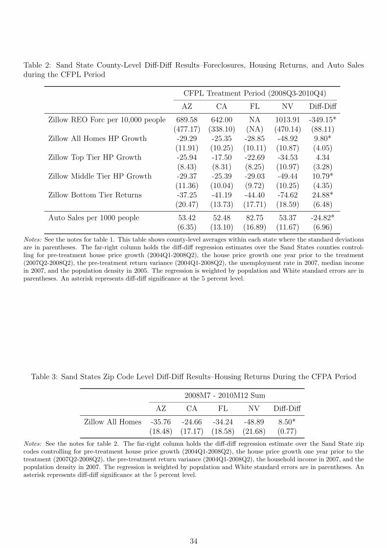
Table 2: Sand State County-Level Diff-Diff Results–Foreclosures, Housing Returns, and Auto Salesduring the CFPL Period

CFPL Treatment Period (2008Q3-2010Q4)

AZ CA FL NV Diff-Diff

Zillow REO Forc per 10,000 people 689.58 642.00 NA 1013.91 -349.15*(477.17) (338.10) (NA) (470.14) (88.11)

Zillow All Homes HP Growth -29.29 -25.35 -28.85 -48.92 9.80*(11.91) (10.25) (10.11) (10.87) (4.05)

Zillow Top Tier HP Growth -25.94 -17.50 -22.69 -34.53 4.34(8.43) (8.31) (8.25) (10.97) (3.28)

Zillow Middle Tier HP Growth -29.37 -25.39 -29.03 -49.44 10.79*(11.36) (10.04) (9.72) (10.25) (4.35)

Zillow Bottom Tier Returns -37.25 -41.19 -44.40 -74.62 24.88*(20.47) (13.73) (17.71) (18.59) (6.48)

Auto Sales per 1000 people 53.42 52.48 82.75 53.37 -24.82*(6.35) (13.10) (16.89) (11.67) (6.96)

Notes: See the notes for table 1. This table shows county-level averages within each state where the standard deviationsare in parentheses. The far-right column holds the diff-diff regression estimates over the Sand States counties control-ling for pre-treatment house price growth (2004Q1-2008Q2), the house price growth one year prior to the treatment(2007Q2-2008Q2), the pre-treatment return variance (2004Q1-2008Q2), the unemployment rate in 2007, median incomein 2007, and the population density in 2005. The regression is weighted by population and White standard errors are inparentheses. An asterisk represents diff-diff significance at the 5 percent level.

Table 3: Sand States Zip Code Level Diff-Diff Results–Housing Returns During the CFPA Period

2008M7 - 2010M12 Sum

AZ CA FL NV Diff-Diff

Zillow All Homes -35.76 -24.66 -34.24 -48.89 8.50*(18.48) (17.17) (18.58) (21.68) (0.77)

Notes: See the notes for table 2. The far-right column holds the diff-diff regression estimate over the Sand State zipcodes controlling for pre-treatment house price growth (2004Q1-2008Q2), the house price growth one year prior to thetreatment (2007Q2-2008Q2), the pre-treatment return variance (2004Q1-2008Q2), the household income in 2007, and thepopulation density in 2007. The regression is weighted by population and White standard errors are in parentheses. Anasterisk represents diff-diff significance at the 5 percent level.

34

Table 4: State-Level Synthetic Control Unit Weights

Outcome Variable Controls Synth Weights

Forc Starts (% of All Loans) 42 NV: 0.47; MD: 0.31; FL: 0.22Prime Forc Starts (% of Prime Loans) 42 NV: 0.59; MD: 0.20; AZ: 0.17; FL: 0.04Subprime Forc Starts (% of Subprime Loans) 42 NV: 0.98; FL: 0.02Zillow REO Forc per 10,000 people 21 NV: 0.68; MA: 0.32Growth in Housing Distress (HDI) 20 FL: 0.46; MA: 0.42; MD: 0.10; MI: 0.02

FHFA HP Growth 42 NV: 0.58; FL: 0.39; MI: 0.02Zillow All Homes HP Growth 37 NV: 0.41; FL: 0.36; MI: 0.23Zillow Top Tier HP Growth 39 NV: 0.33; VA: 0.27; MA: 0.16; MI: 0.11;

WA: 0.09; FL: 0.03; MD: 0.00Zillow Middle Tier HP Growth 37 NV: 0.42; FL: 0.27; MN: 0.23; MA: 0.08Zillow Bottom Tier HP Growth 38 NV: 0.60; MA: 0.22; FL: 0.17; MN: 0.02

Auto Sales per 1000 people 42 FL: 0.36; KY: 0.27; AZ: 0.22; AR: 0.08;MA: 0.03; MS: 0.02; MI: 0.01

Notes: The Synthetic Control unit weights. The left column lists the outcome variable, the middle column shows thenumber of available controls, and the right column shows Synthetic Control weights. Only states weights with positiveweight are listed.

Table 5: State-Level Synthetic Control Estimation Results

CFPL Treatment Period (2008Q3-2010Q4)

Outcome Variable RMSFE California Synthetic Gap Percentile

Forc Starts (% of All Loans) 0.01 15.96 23.23 -7.27*** 2.33Prime Forc Starts (% of Prime Loans) 0.00 12.90 21.11 -8.21*** 2.33Subprime Forc Starts (% of Subprime Loans) 0.03 45.71 66.07 -20.36*** 2.70Zillow REO Forc per 10,000 people 0.96 640.26 871.00 -230.73** 5.00Growth in Housing Distress (HDI) 0.01 -68.00 -45.09 -16.88* 10.53

FHFA HP Growth 0.40 -20.19 -37.96 17.77*** 100.00Zillow All Homes HP Growth 0.03 -22.03 -37.33 15.30*** 100.00Zillow Top Tier HP Growth 0.03 -9.14 -18.97 9.83** 90.32Zillow Middle Tier HP Growth 0.03 -16.19 -35.07 18.87*** 100.00Zillow Bottom Tier HP Growth 0.06 -40.26 -61.19 20.93*** 100.00Auto Sales per 1000 people 0.17 60.82 69.71 -8.90** 5.13

Notes: State-level estimates from the Synthetic Control procedure. The left column lists the outcome variable, RMSFEis the root mean-squared forecast error from the Synthetic control match during the pre-treatment period, the nexttwo columns show the change in the outcome variable during the CFPL treatment period (2008Q3-2010Q4; 2008M7-2010M12), and Gap is the difference between of the change in the outcome variable for Treated Unit (California) relativeto its Synthetic Control. The far right column shows the percentile of the Gap estimate relative to all placebo effects.One, two, and three asterisks indicates that the Gap estimate for the treated unit is the greater (lower) than the 85, 90,and 95th (5, 10, and 15th) percentiles of all estimated placebo effects.

35

Tab

le6:

Cou

nty

-Lev

elSynth

etic

Con

trol

Est

imat

es

Zillow

Foreclosu

res

Zillow

AllHomes

Zillow

TopTier

Zillow

Middle

Tier

County

RMSFE

Gap

Percentile

RMSFE

Gap

Percentile

RMSFE

Gap

Percentile

RMSFE

Gap

Percentile

Alamed

a6001

0.56

126.43

94.12

0.05

11.16**

91.73

0.07

-0.63

36.79

0.11

0.64

41.70

Butte6

007

NA

NA

NA

0.38

12.21**

94.17

0.20

3.18

63.77

0.23

15.22***

98.46

ContraCosta6013

1.65

-218.07***

4.58

0.04

-10.65

4.70

0.07

0.31

44.53

0.07

-3.04

19.88

ElD

orado6017

NA

NA

NA

0.08

-12.14

3.95

0.10

-8.13

7.17

0.13

-9.10

4.83

Fresn

o6019

1.01

-178.63**

6.54

0.18

-0.19

39.10

0.18

2.61

58.87

0.19

-1.55

28.19

Humboldt6023

NA

NA

NA

0.42

-6.23

11.84

0.56

-9.91

4.72

0.39

-4.48

13.71

Imperial6025

NA

NA

NA

0.69

-21.87

1.13

0.29

-13.31

2.08

0.21

-17.75

0.97

Kern6029

1.40

-494.81***

0.65

0.24

-2.29

26.32

0.21

0.49

46.04

0.26

-4.90

12.36

Kings6031

0.74

-73.47

24.18

0.27

4.92

71.24

0.47

10.58**

93.02

0.30

4.43

68.73

Lake6

033

1.31

-15.70

48.37

0.56

-4.80

15.23

0.88

-23.87

0.38

0.49

-8.74

4.83

LosA

ngeles6037

1.33

-174.91**

6.54

0.20

14.83***

96.24

0.14

6.78

81.51

0.18

8.95*

88.03

Madera6039

NA

NA

NA

0.76

-1.47

30.45

0.70

-3.72

18.87

0.73

-3.07

19.88

Marin6041

NA

NA

NA

0.08

-1.81

29.14

0.18

-3.93

18.68

0.09

-9.49

4.63

Men

docino6045

NA

NA

NA

1.92

-0.37

37.59

0.59

7.41

84.34

1.56

2.12

53.67

Monterey6053

NA

NA

NA

0.66

-0.42

36.47

0.47

9.52**

90.94

0.84

7.23

82.82

Napa6055

NA

NA

NA

0.20

-7.54

8.27

0.14

-1.66

31.51

0.17

-10.14

4.25

Nevada6057

NA

NA

NA

0.10

6.64

77.82

0.16

-3.45

20.00

0.11

0.29

39.77

Orange6

059

0.52

-103.65*

11.76

0.32

7.10

80.26

0.28

-1.72

31.32

0.31

5.70

76.45

Placer6061

NA

NA

NA

0.22

-10.83

4.70

0.10

-7.31

8.49

0.11

-7.56

6.95

Riverside6

065

5.22

154.07

95.42

0.36

-3.95

17.86

0.19

2.81

60.57

0.29

-7.26

7.92

Sacramen

to6067

5.31

55.49

86.93

0.15

-0.76

35.15

0.12

2.90

61.13

0.10

0.66

41.89

SanBernard

ino6071

2.75

-256.68***

1.31

0.27

-1.42

30.64

0.09

13.51***

96.42

0.08

11.66**

94.40

SanDiego6073

2.72

-156.39**

6.54

0.33

2.94

59.77

0.31

3.33

64.72

0.38

6.13

77.80

SanFrancisco6075

NA

NA

NA

0.37

6.39

76.69

0.30

-0.95

35.66

0.26

-0.76

33.59

SanJoaquin6077

36.09

533.37

100.00

0.24

1.38

50.75

0.43

-7.00

8.87

0.31

-4.70

13.32

SanLuisObispo6079

NA

NA

NA

0.50

-20.49

1.50

0.35

2.02

56.60

0.30

-15.34

1.16

SanMateo6081

0.18

4.52

62.09

0.12

-0.33

37.97

0.19

-2.40

26.23

0.16

-9.57

4.63

SantaBarb

ara6083

NA

NA

NA

0.30

4.16

66.35

0.33

3.33

64.72

0.31

6.32

78.57

SantaClara6085

2.38

-2.50

54.25

0.04

-1.17

32.71

0.08

-0.65

36.42

0.06

2.63

57.34

SantaCru

z6087

NA

NA

NA

0.26

14.31***

95.68

0.16

-6.21

10.57

0.28

11.06**

92.86

Shasta6089

2.46

7.08

63.40

0.49

-11.00

4.70

0.19

4.40

72.08

0.29

-3.56

17.18

Solano6095

1.57

-135.21**

8.50

0.21

-12.61

3.76

0.12

-9.84

4.91

0.15

-17.18

0.97

Sonoma6097

1.19

-252.64***

1.31

0.18

3.00

60.53

0.14

0.39

45.09

0.21

-1.40

29.34

Stanislaus6099

9.80

492.65

99.35

0.19

-4.64

15.60

0.25

-15.18

1.32

0.19

-7.44

7.14

Sutter6101

NA

NA

NA

0.77

-13.48

2.82

0.68

-12.82

2.08

0.70

-6.25

9.27

Tulare6107

0.23

-123.21**

9.80

0.45

9.79*

88.53

0.31

-0.53

37.92

0.34

10.80**

92.86

Ven

tura6111

0.62

-83.67

21.57

0.23

2.31

57.71

0.28

5.85

78.49

0.23

4.71

71.04

Yolo6113

NA

NA

NA

1.25

-6.03

12.41

0.51

9.61**

91.32

0.85

-7.27

7.72

Yuba6115

NA

NA

NA

1.10

5.95

75.00

0.80

-1.52

31.70

0.62

3.87

65.44

Notes:

Cou

nty

-lev

eles

tim

ates

from

the

Synth

etic

Con

trol

pro

ced

ure

wh

ere

ou

tcom

eva

riab

les

are

retu

rns

on

the

Zil

low

All

Hom

es,

Top

Tie

r,M

idd

leT

ier,

Bott

om

Tie

r,an

dC

ond

omin

ium

Hou

sep

rice

ind

ices

and

auto

sale

sp

er10

00p

eop

le.

Wit

hin

each

pan

el,

we

show

the

pre

-tre

atm

ent

RM

SF

E,

the

Gap

Est

imate

,an

dth

eG

ap

Per

centi

lere

lati

veto

all

pla

ceb

oeff

ects

.T

he

FIP

Sco

de

for

each

cou

nty

isap

pen

ded

toth

eco

unty

nam

e.

36

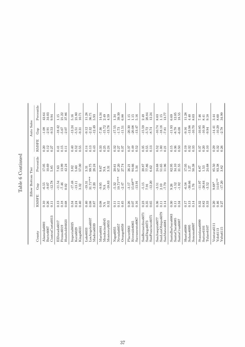
Tab

le6

Con

tinued

Zillow

Bottom

Tier

Auto

Sales

County

RMSFE

Gap

Percentile

RMSFE

Gap

Percentile

Alamed

a6001

0.10

-6.55

17.05

0.20

-1.08

42.64

Butte6

007

0.26

-9.07

10.69

0.12

-2.91

34.03

ContraCosta6013

0.11

-12.78

5.85

0.27

-9.53

9.94

ElD

orado6017

0.13

-11.54

7.63

0.41

-18.42

1.15

Fresn

o6019

0.18

-7.46

13.99

0.15

-5.67

21.22

Humboldt6023

0.68

0.02

42.24

0.11

-2.07

37.86

Imperial6025

0.34

-17.48

3.82

0.40

-13.24

5.16

Kern6029

0.24

-13.11

5.60

0.52

-5.51

21.80

Kings6031

0.40

3.32

57.00

0.55

-9.31

10.71

Lake6

033

0.40

-19.31

3.31

0.14

-9.12

11.28

LosA

ngeles6037

0.08

31.71***

99.75

0.13

-2.32

36.71

Madera6039

0.87

-2.20

28.24

0.43

-12.49

5.93

Marin6041

0.08

-9.95

9.67

0.33

-7.36

14.34

Men

docino6045

NA

NA

NA

0.25

-15.72

2.49

Monterey6053

0.32

-18.83

3.31

0.24

-13.78

4.59

Napa6055

0.11

-5.32

20.61

0.32

-17.55

1.34

Nevada6057

0.11

19.71***

97.20

0.27

-1.73

39.39

Orange6

059

0.45

-2.47

27.74

0.37

-11.51

6.88

Placer6061

0.26

-3.17

26.21

0.37

-20.30

1.15

Riverside6

065

0.07

15.68**

94.66

0.49

-20.08

1.15

Sacramen

to6067

0.16

-13.91

5.34

0.52

-13.47

5.16

SanBernard

ino6071

0.23

-5.15

20.87

0.35

-15.59

2.49

SanDiego6073

0.35

7.91

77.86

0.55

-5.72

20.84

SanFrancisco6075

0.65

-12.20

6.62

0.13

-8.74

12.24

SanJoaquin6077

0.36

-3.51

24.68

0.52

-10.74

8.03

SanLuisObispo6079

0.11

2.10

51.65

1.00

-18.18

1.15

SanMateo6081

0.14

-7.79

11.96

0.21

-7.81

13.77

SantaBarb

ara6083

0.30

9.26

82.95

0.15

-11.93

6.69

SantaClara6085

0.11

-1.52

34.10

0.36

-8.78

12.05

SantaCru

z6087

0.34

-1.92

31.55

0.50

-6.08

18.55

Shasta6089

0.17

-6.58

17.05

0.19

-9.16

11.28

Solano6095

0.13

-30.66

1.27

0.32

-13.98

4.40

Sonoma6097

0.14

1.76

50.38

0.33

-10.70

8.03

Stanislaus6099

0.32

-11.97

6.87

0.37

-10.85

7.46

Sutter6101

0.82

-26.64

1.53

0.20

-10.30

8.41

Tulare6107

0.33

-3.52

24.68

0.10

-9.94

9.18

Ven

tura6111

0.20

9.68*

85.50

0.29

-14.41

3.44

Yolo6113

0.46

14.01**

93.38

0.32

-10.29

8.60

Yuba6115

0.27

-17.20

3.82

0.26

-2.78

34.99

37

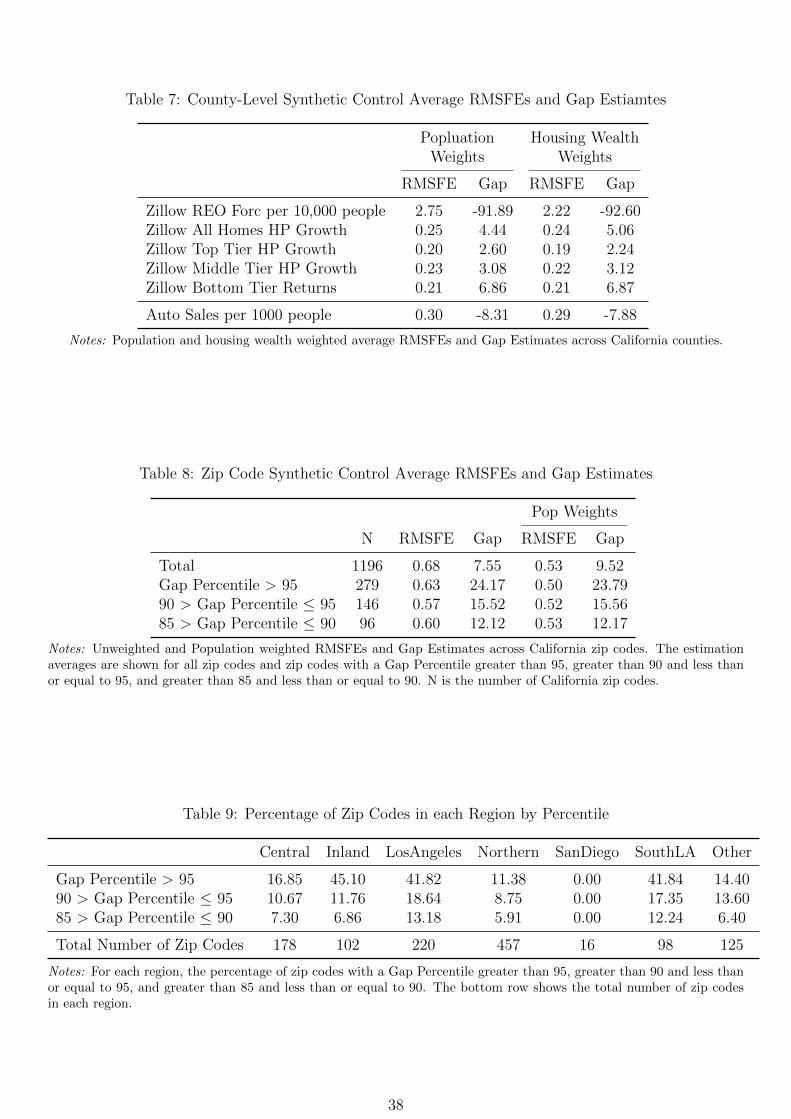
Table 7: County-Level Synthetic Control Average RMSFEs and Gap Estiamtes

PopluationWeights

Housing WealthWeights

RMSFE Gap RMSFE Gap

Zillow REO Forc per 10,000 people 2.75 -91.89 2.22 -92.60Zillow All Homes HP Growth 0.25 4.44 0.24 5.06Zillow Top Tier HP Growth 0.20 2.60 0.19 2.24Zillow Middle Tier HP Growth 0.23 3.08 0.22 3.12Zillow Bottom Tier Returns 0.21 6.86 0.21 6.87

Auto Sales per 1000 people 0.30 -8.31 0.29 -7.88

Notes: Population and housing wealth weighted average RMSFEs and Gap Estimates across California counties.

Table 8: Zip Code Synthetic Control Average RMSFEs and Gap Estimates

Pop Weights

N RMSFE Gap RMSFE Gap

Total 1196 0.68 7.55 0.53 9.52Gap Percentile > 95 279 0.63 24.17 0.50 23.7990 > Gap Percentile ≤ 95 146 0.57 15.52 0.52 15.5685 > Gap Percentile ≤ 90 96 0.60 12.12 0.53 12.17

Notes: Unweighted and Population weighted RMSFEs and Gap Estimates across California zip codes. The estimationaverages are shown for all zip codes and zip codes with a Gap Percentile greater than 95, greater than 90 and less thanor equal to 95, and greater than 85 and less than or equal to 90. N is the number of California zip codes.

Table 9: Percentage of Zip Codes in each Region by Percentile

Central Inland LosAngeles Northern SanDiego SouthLA Other

Gap Percentile > 95 16.85 45.10 41.82 11.38 0.00 41.84 14.4090 > Gap Percentile ≤ 95 10.67 11.76 18.64 8.75 0.00 17.35 13.6085 > Gap Percentile ≤ 90 7.30 6.86 13.18 5.91 0.00 12.24 6.40

Total Number of Zip Codes 178 102 220 457 16 98 125

Notes: For each region, the percentage of zip codes with a Gap Percentile greater than 95, greater than 90 and less thanor equal to 95, and greater than 85 and less than or equal to 90. The bottom row shows the total number of zip codesin each region.

38

B Figures

39

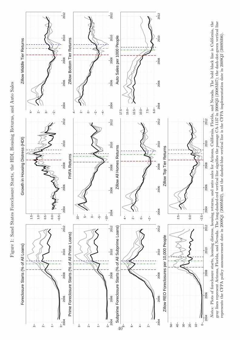
Fig

ure

1:San

dSta

tes

For

eclo

sure

Sta

rts,

the

HD

I,H

ousi

ng

Ret

urn

s,an

dA

uto

Sal

es

0123

2004

2006

2008

2010

2012

For

eclo

sure

Sta

rts

(% o

f All

Loan

s)

0123

2004

2006

2008

2010

2012

Prim

e F

orec

losu

re S

tart

s (%

of A

ll P

rime

Loan

s)

2468

2004

2006

2008

2010

2012

Sub

prim

e F

orec

losu

re S

tart

s (%

of A

ll S

ubpr

ime

Loan

s)

01020304050

2004

2006

2008

2010

2012

Zill

ow R

EO

For

eclo

sure

s pe

r 10

,000

Peo

ple

−0.

5

0.0

0.5

1.0

1.5

2004

2006

2008

2010

2012

Gro

wth

in H

ousi

ng D

istr

ess

(HD

I)

−10−

50510

2004

2006

2008

2010

2012

FH

FA R

etur

ns

−2024

2004

2006

2008

2010

2012

Zill

ow A

ll H

omes

Ret

urns

−2.

5

0.0

2.5

2004

2006

2008

2010

2012

Zill

ow T

op T

ier

Ret

urns

−2024

2004

2006

2008

2010

2012

Zill

ow M

iddl

e T

ier

Ret

urns

−4

−2024

2004

2006

2008

2010

2012

Zill

ow B

otto

m T

ier

Ret

urns

5.0

7.5

10.0

12.5

15.0

17.5

2004

2006

2008

2010

2012

Aut

o S

ales

per

100

0 P

eopl

e

Notes:

Plo

tsof

fore

clos

ure

star

ts,

hou

sin

gd

istr

ess,

hou

sin

gre

turn

s,an

dau

tosa

les

for

Ari

zon

a,

Cali

forn

ia,

Flo

rid

a,

an

dN

evad

a.

Th

eb

old

bla

cklin

eis

Cali

forn

ia,

the

gray

lin

esre

pre

sent

Ari

zon

a,F

lori

da,

and

Nev

ada.

Th

elo

ng-

das

hed

-red

vert

ical

lin

esi

gn

ifies

the

pass

age

CA

-1137

in2008Q

3(2

008M

07);

the

dash

-dot-

gre

enve

rtic

al

line

rep

rese

nts

the

CF

PA

pol

icy

ann

oun

cem

ent

dat

ein

2009

Q1

(200

9M

02),

an

dth

ed

ash

ed-b

lue

vert

ical

lin

eis

the

CF

PA

imp

lem

enta

tion

date

in2009Q

2(2

009M

06).

40

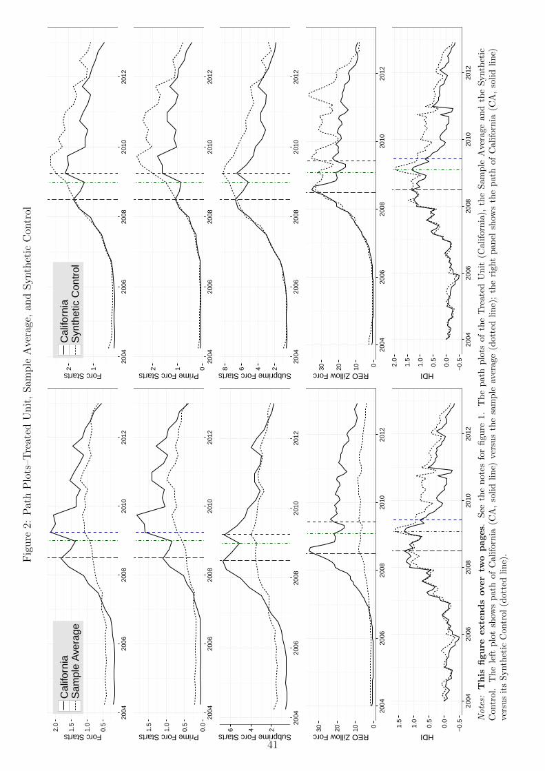
Fig

ure

2:P

ath

Plo

ts–T

reat

edU

nit

,Sam

ple

Ave

rage

,an

dSynth

etic

Con

trol

0.5

1.0

1.5

2.0

2004

2006

2008

2010

2012

Forc Starts

Cal

iforn

iaS

ampl

e A

vera

ge

0.0

0.5

1.0

1.5

2004

2006

2008

2010

2012

Prime Forc Starts 246

2004

2006

2008

2010

2012

Subprime Forc Starts

0102030

2004

2006

2008

2010

2012

REO Zillow Forc −0.

5

0.0

0.5

1.0

1.5

2004

2006

2008

2010

2012

HDI

12

2004

2006

2008

2010

2012

Forc Starts

Cal

iforn

iaS

ynth

etic

Con

trol

012

2004

2006

2008

2010

2012

Prime Forc Starts 2468

2004

2006

2008

2010

2012

Subprime Forc Starts

0102030

2004

2006

2008

2010

2012

REO Zillow Forc −0.

5

0.0

0.5

1.0

1.5

2.0

2004

2006

2008

2010

2012

HDI

Notes:

Th

isfi

gu

reexte

nd

sover

two

pages.

See

the

not

esfo

rfi

gu

re1.

Th

ep

ath

plo

tsof

the

Tre

ate

dU

nit

(Cali

forn

ia),

the

Sam

ple

Aver

age

an

dth

eS

ynth

etic

Con

trol

.T

he

left

plo

tsh

ows

pat

hof

Cal

ifor

nia

(CA

,so

lid

lin

e)ve

rsu

sth

esa

mp

leav

erage

(dott

edli

ne)

;th

eri

ght

pan

elsh

ows

the

path

of

Cali

forn

ia(C

A,

soli

dli

ne)

vers

us

its

Synth

etic

Con

trol

(dot

ted

lin

e).

41

Fig

ure

2C

onti

nued

−50510

2004

2006

2008

2010

2012

FHFA Returns −2

−1012

2004

2006

2008

2010

2012

Zillow All Homes −1012

2004

2006

2008

2010

2012

Zillow Top Teir −2

−1012

2004

2006

2008

2010

2012

Zillow Middle Tier −3

−2

−1012

2004

2006

2008

2010

2012

Zillow Bottom Tier

5791113

2004

2006

2008

2010

2012

Auto Sales

−10−

50510

2004

2006

2008

2010

2012

FHFA Returns −2

−1012

2004

2006

2008

2010

2012

Zillow All Homes −1012

2004

2006

2008

2010

2012

Zillow Top Teir −2

−1012

2004

2006

2008

2010

2012

Zillow Middle Tier −202

2004

2006

2008

2010

2012

Zillow Bottom Tier

681012

2004

2006

2008

2010

2012

Auto Sales

42

Figure 3: California County-Level Gap in House Price Growth and Auto Sales

ContraCosta***

Fresno***

Kern***

LosAngeles***

Orange***

SanBernardino***

SanDiego***

Solano***Sonoma***

Tulare***

−250

0

250

500

Gap in Zillow REO Forc per 10,000 people

Kings**Monterey**

SanBernardino***

Yolo**

−20

−10

0

10

Gap in Zillow Top Tier HP Growth

Alameda**

Butte**

LosAngeles***

SantaCruz***

Tulare*

−20

−10

0

10

Gap in Zillow All Homes HP Growth

Butte***

LosAngeles*SanBernardino**

SantaCruz**

Tulare**

−10

0

10

Gap in Zillow Middle Tier HP Growth

Notes: Continued on next page. Choropleth plots of the Gap in California county-level house pricegrowth and auto sales during the CFPA period.

43

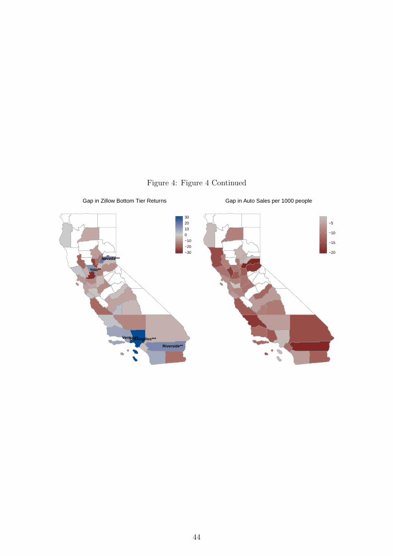
Figure 4: Figure 4 Continued

LosAngeles***

Nevada***

Riverside**

Ventura*

Yolo**

−30

−20

−10

0

10

20

30

Gap in Zillow Bottom Tier Returns

−20

−15

−10

−5

Gap in Auto Sales per 1000 people

44

Fig

ure

5:P

ath

Plo

ts–L

osA

nge

les

Cou

nty

,Sam

ple

Ave

rage

,an

dSynth

etic

Con

trol

01020

2004

2006

2008

2010

2012

Zillow REO Forc

Los

Ang

eles

Cou

nty

Sam

ple

Ave

rage

−2

−1012

2004

2006

2008

2010

2012

Zillow All Homes

791113

2004

2006

2008

2010

2012

Auto Sales

01020

2004

2006

2008

2010

2012

Zillow REO Forc

Los

Ang

eles

Cou

nty

Syn

thet

ic C

ontr

ol

−2

−1012

2004

2006

2008

2010

2012

Zillow All Homes

791113

2004

2006

2008

2010

2012

Auto Sales

Notes:

Pat

hp

lots

for

Los

An

gele

sC

ounty

for

Zil

low

RE

OF

ore

closu

res

per

10,0

00

peo

ple

,Z

illo

wA

llH

om

esre

turn

s,an

dau

tosa

les

per

1000

peo

ple

.T

he

left

plo

tsh

ows

pat

hof

Los

An

gele

s(s

olid

lin

e)ve

rsu

sth

esa

mp

leav

erage

(dott

edli

ne)

;th

eri

ght

pan

elsh

ows

the

path

of

Los

An

gel

esC

ou

nty

(soli

dli

ne)

vers

us

its

Synth

etic

Con

trol

(dot

ted

lin

e).

Th

elo

ng-

das

hed

-red

vert

ical

lin

esi

gnifi

esth

ep

ass

age

CA

-1137

in2008Q

3(2

008M

07);

the

dash

-dot-

gre

enve

rtic

al

lin

ere

pre

sents

the

CF

PA

policy

ann

oun

cem

ent

dat

ein

2009

Q1

(200

9M02

),an

dth

ed

ash

ed-b

lue

vert

ical

lin

eis

the

CF

PA

imp

lem

enta

tion

date

in2009Q

2(2

009M

06).

45

C Appendix: Data List

46

Tab

le10

:D

ata

Lis

t

Mnem

onic

Des

crip

tion

Fre

quen

cySou

rce

Sta

te-L

evel

Dat

a

For

eclo

sure

Sta

rts–

Per

centa

geof

loan

sth

aten

ter

fore

clos

ure

QM

BA

Pri

me

For

elco

sure

Sta

rts

QM

BA

Subpri

me

For

eclo

sure

Sta

rts

QM

BA

Hou

sing

Dis

tres

sIn

dex

(HD

I)M

CG

LF

HFA

Hou

seR

eturn

sQ

FH

FA

Zillo

wR

eturn

s(A

llH

omes

,T

opT

ier,

Mid

dle

Tie

r,B

otto

mT

ier,

Con

dos

)M

Zillo

wA

uto

Sal

esP

er10

00P

eople

QP

olk

**B

P1F

HSA

Hou

sing

Sta

rts

QF

RE

D**

NA

Non

farm

Pay

rolls

QF

RE

D**

OT

OT

Tot

alP

erso

nal

Inco

me

QF

RE

DSai

zE

last

icit

yN

ASai

z**

PO

PP

opula

tion

Den

sity

in20

05N

AF

RE

D,C

ensu

s

Cou

nty

-Lev

elD

ata

Zillo

wR

eturn

s(A

llH

omes

,T

opT

ier,

Mid

dle

Tie

r,B

otto

mT

ier,

Con

dos

)M

Zillo

wA

uto

Sal

esP

er10

00P

eople

QP

olk

Med

ian

Hou

sehol

dIn

com

eY

AC

SU

nem

plo

ym

ent

Rat

eY

BL

SP

opula

tion

Den

sity

in20

05N

AA

CS,C

ensu

s

Zip

Code

Lev

elD

ata

Zillo

wR

eturn

s(A

llH

omes

)M

Zillo

wIn

com

ep

erhou

sehol

dN

AIR

SP

opula

tion

Den

sity

in20

07N

AIR

S,C

ensu

s

Notes:

MB

Ais

the

Mor

tgag

eB

anke

rs’

Ass

oci

atio

n;

CG

Lis

Ch

au

vet,

Gab

riel

,an

dL

utz

(2015);

FR

ED

isth

eF

RE

DD

ata

base

of

the

Fed

eral

Res

erve

Ban

kof

St.

Lou

is;

Cen

sus

isth

eU

SC

ensu

s;A

CS

isth

eA

mer

ican

Com

mu

nit

yS

urv

ey;

BL

Sis

the

Bu

reau

of

Lab

or

Sta

tist

ics;

IRS

isth

eIR

SS

tati

stic

sof

Inco

me.

47

Table 11: California Counties and FIPs codes

Alameda - 6001 Sacramento - 6067Butte - 6007 San Bernardino - 6071Contra Costa - 6013 San Diego - 6073El Dorado - 6017 San Francisco - 6075Fresno - 6019 San Joaquin - 6077Humboldt - 6023 San Luis Obispo - 6079Imperial - 6025 San Mateo - 6081Kern - 6029 Santa Barbara - 6083Kings - 6031 Santa Clara - 6085Lake - 6033 Santa Cruz - 6087Los Angeles - 6037 Shasta - 6089Madera - 6039 Solano - 6095Marin - 6041 Sonoma - 6097Mendocino - 6045 Stanislaus - 6099Monterey - 6053 Sutter - 6101Napa - 6055 Tulare - 6107Nevada - 6057 Ventura - 6111Orange - 6059 Yolo - 6113Placer - 6061 Yuba - 6115Riverside - 6065

48