Embed Size (px)
DESCRIPTION
A textbook about error-correcting codes. Written by Jørn Justesen and Tom Høholdt, Technical University of Denmark (DTU)
Citation preview

S
E
EM
SM E M S
SS
E
EM
SS
E
EM MM
ETB_justesen_titelei.qxd 14.01.2004 9:36 Uhr Seite 1

EMS Textbooks in Mathematics
EMS Textbooks in Mathematics is a book series aimed at students or professional mathematicians seeking anintroduction into a particular field. The individual volumes are intended to provide not only relevant techniques,results and their applications, but afford insight into the motivations and ideas behind the theory. Suitablydesigned exercises help to master the subject and prepare the reader for the study of more advanced and spe-cialized literature.
ETB_justesen_titelei.qxd 14.01.2004 9:36 Uhr Seite 2
Jørn JustesenTom Høholdt
A Course In Error-Correcting Codes
SS
E
EM
SS
E
EM MM European Mathematical Society
S
E
EM
SM
ETB_justesen_titelei.qxd 14.01.2004 9:36 Uhr Seite 3

Authors:
Jørn Justesen Tom HøholdtCOM Department of MathematicsTechnical University of Denmark Technical University of DenmarkBldg.371 Bldg. 303DK-2800 Kgs. Lyngby DK-2800 Kgs. LyngbyDenmark Denmark
2000 Mathematics Subject Classification 94-01;12-01
Bibliographic information published by Die Deutsche Bibliothek
Die Deutsche Bibliothek lists this publication in the Deutsche Nationalbibliografie; detailed bibliographic data are available in the Internet at http://dnb.ddb.de.
ISBN 3-03719-001-9
This work is subject to copyright. All rights are reserved, whether the whole or part of the material is concerned, specifically the rights of translation, reprinting, re-use of illustrations, recitation, broadcasting,reproduction on microfilms or in other ways, and storage in data banks. For any kind of use permission of the copyright owner must be obtained.
© 2004 European Mathematical Society
Contact address:
European Mathematical Society Publishing HouseSeminar for Applied MathematicsETH-Zentrum FLI C1CH-8092 ZürichSwitzerland
Phone: +41 (0)1 632 34 36Email: [email protected]: www.ems-ph.org
Printed on acid-free paper produced from chlorine-free pulp. TCF ∞Printed in Germany
9 8 7 6 5 4 3 2 1
ETB_justesen_titelei.qxd 14.01.2004 9:36 Uhr Seite 4
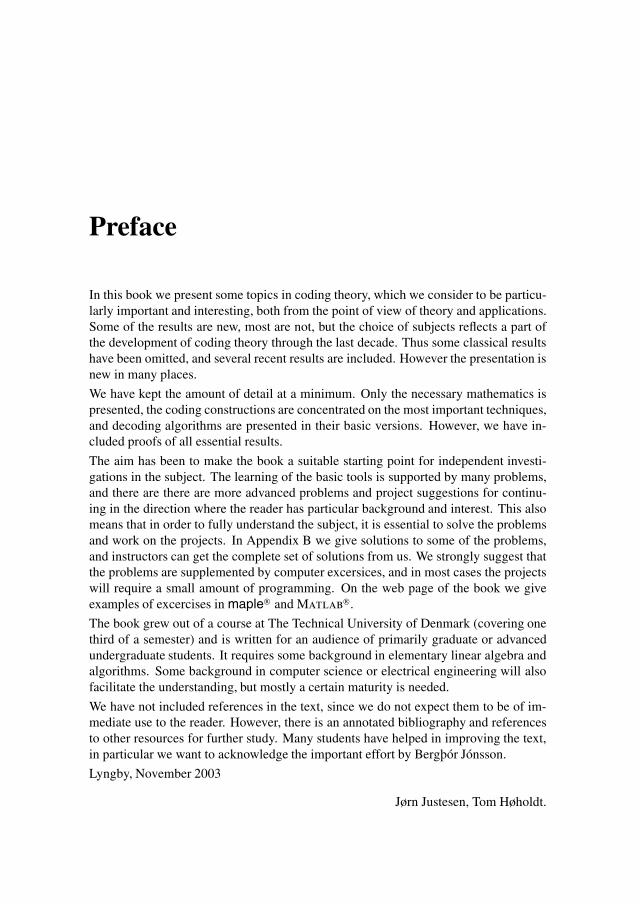
Contents
Preface . . . . . . . . . . . . . . . . . . . . . . . . . . . . . . . . . . . . . . ix
1 Block codes for error-correction1.1 Linear codes and vector spaces . . . . . . . . . . . . . . . . . . . . . 11.2 Minimum distance and minimum weight . . . . . . . . . . . . . . . . 41.3 Syndrome decoding and the Hamming bound . . . . . . . . . . . . . 81.4 Weight distributions . . . . . . . . . . . . . . . . . . . . . . . . . . . 111.5 Problems . . . . . . . . . . . . . . . . . . . . . . . . . . . . . . . . 13
2 Finite fields2.1 Fundamental properties of finite fields . . . . . . . . . . . . . . . . . 192.2 The finite field F2m . . . . . . . . . . . . . . . . . . . . . . . . . . . 222.3 Minimal polynomials and factorization of xn − 1 . . . . . . . . . . . 252.4 Problems . . . . . . . . . . . . . . . . . . . . . . . . . . . . . . . . 29
3 Bounds on error probability for error-correcting codes3.1 Some probability distributions . . . . . . . . . . . . . . . . . . . . . 333.2 The probability of failure and error for bounded distance decoding . . 343.3 Bounds for maximum likelihood decoding of binary block codes . . . 373.4 Problems . . . . . . . . . . . . . . . . . . . . . . . . . . . . . . . . 39
4 Communication channels and information theory4.1 Discrete messages and entropy . . . . . . . . . . . . . . . . . . . . . 414.2 Mutual information and capacity of discrete channels . . . . . . . . . 42
4.2.1 Discrete memoryless channels . . . . . . . . . . . . . . . . . 424.2.2 Codes and channel capacity . . . . . . . . . . . . . . . . . . 45
4.3 Problems . . . . . . . . . . . . . . . . . . . . . . . . . . . . . . . . 47
5 Reed-Solomon codes and their decoding5.1 Basic definitions . . . . . . . . . . . . . . . . . . . . . . . . . . . . . 495.2 Decoding Reed-Solomon Codes . . . . . . . . . . . . . . . . . . . . 515.3 Vandermonde matrices . . . . . . . . . . . . . . . . . . . . . . . . . 535.4 Another decoding algorithm . . . . . . . . . . . . . . . . . . . . . . 575.5 Problems . . . . . . . . . . . . . . . . . . . . . . . . . . . . . . . . 61

vi Contents
6 Cyclic Codes6.1 Introduction to cyclic codes . . . . . . . . . . . . . . . . . . . . . . . 636.2 Generator- and parity check matrices of cyclic codes . . . . . . . . . 656.3 A theorem on the minimum distance of cyclic codes . . . . . . . . . . 666.4 Cyclic Reed-Solomon codes and BCH-codes . . . . . . . . . . . . . 67
6.4.1 Cyclic Reed-Solomon codes . . . . . . . . . . . . . . . . . . 686.4.2 BCH-codes . . . . . . . . . . . . . . . . . . . . . . . . . . . 68
6.5 Problems . . . . . . . . . . . . . . . . . . . . . . . . . . . . . . . . 70
7 Frames7.1 Definitions of frames and their efficiency . . . . . . . . . . . . . . . . 737.2 Frame quality . . . . . . . . . . . . . . . . . . . . . . . . . . . . . . 76
7.2.1 Measures of quality . . . . . . . . . . . . . . . . . . . . . . . 767.2.2 Parity checks on frames . . . . . . . . . . . . . . . . . . . . 76
7.3 Error detection and error correction . . . . . . . . . . . . . . . . . . 777.3.1 Short block codes . . . . . . . . . . . . . . . . . . . . . . . . 777.3.2 Convolutional codes . . . . . . . . . . . . . . . . . . . . . . 797.3.3 Reed-Solomon codes . . . . . . . . . . . . . . . . . . . . . . 797.3.4 Low density codes and ‘turbo’ codes . . . . . . . . . . . . . . 80
7.4 Problems . . . . . . . . . . . . . . . . . . . . . . . . . . . . . . . . 80
8 Convolutional codes8.1 Parameters of convolutional codes . . . . . . . . . . . . . . . . . . . 838.2 Tail-biting codes . . . . . . . . . . . . . . . . . . . . . . . . . . . . 868.3 Parity checks and dual codes . . . . . . . . . . . . . . . . . . . . . . 878.4 Distances of convolutional codes . . . . . . . . . . . . . . . . . . . . 898.5 Punctured codes . . . . . . . . . . . . . . . . . . . . . . . . . . . . . 908.6 Linear systems as encoders . . . . . . . . . . . . . . . . . . . . . . . 918.7 Unit memory codes . . . . . . . . . . . . . . . . . . . . . . . . . . . 938.8 Problems . . . . . . . . . . . . . . . . . . . . . . . . . . . . . . . . 95
9 Maximum likelihood decoding of convolutional codes9.1 Finite state descriptions of convolutional codes . . . . . . . . . . . . 979.2 Maximum likelihood decoding . . . . . . . . . . . . . . . . . . . . . 1029.3 Problems . . . . . . . . . . . . . . . . . . . . . . . . . . . . . . . . 106
10 Combinations of several codes10.1 Product codes . . . . . . . . . . . . . . . . . . . . . . . . . . . . . . 10910.2 Concatenated codes (serial encoding) . . . . . . . . . . . . . . . . . 112
10.2.1 Parameters of concatenated codes . . . . . . . . . . . . . . . 11210.2.2 Performance of concatenated codes . . . . . . . . . . . . . . 11310.2.3 Interleaving and inner convolutional codes . . . . . . . . . . 114
10.3 Problems . . . . . . . . . . . . . . . . . . . . . . . . . . . . . . . . 116
11 Decoding Reed-Solomon and BCH-codes with the Euclidian algorithm11.1 The Euclidian algorithm . . . . . . . . . . . . . . . . . . . . . . . . 119

Contents vii
11.2 Decoding Reed-Solomon and BCH codes . . . . . . . . . . . . . . . 12111.3 Problems . . . . . . . . . . . . . . . . . . . . . . . . . . . . . . . . 125
12 List decoding of Reed-Solomon codes12.1 A list decoding algorithm . . . . . . . . . . . . . . . . . . . . . . . . 12712.2 An extended list decoding algorithm . . . . . . . . . . . . . . . . . . 13012.3 Factorization of Q(x, y) . . . . . . . . . . . . . . . . . . . . . . . . 13212.4 Problems . . . . . . . . . . . . . . . . . . . . . . . . . . . . . . . . 135
13 Iterative decoding13.1 Low density parity check codes . . . . . . . . . . . . . . . . . . . . . 13713.2 Iterative decoding of LDPC codes . . . . . . . . . . . . . . . . . . . 13813.3 Decoding product codes . . . . . . . . . . . . . . . . . . . . . . . . 14313.4 Parallel concatenation of convolutional codes (‘turbo codes’) . . . . . 14513.5 Problems . . . . . . . . . . . . . . . . . . . . . . . . . . . . . . . . 149
14 Algebraic geometry codes14.1 Hermitian codes . . . . . . . . . . . . . . . . . . . . . . . . . . . . . 15114.2 Decoding Hermitian codes . . . . . . . . . . . . . . . . . . . . . . . 15514.3 Problems . . . . . . . . . . . . . . . . . . . . . . . . . . . . . . . . 157
A Communication channelsA.1 Gaussian channels . . . . . . . . . . . . . . . . . . . . . . . . . . . . 159A.2 Gaussian channels with quantized input and output . . . . . . . . . . 160A.3 ML Decoding . . . . . . . . . . . . . . . . . . . . . . . . . . . . . . 161
B Solutions to selected problemsB.1 Solutions to problems in Chapter 1 . . . . . . . . . . . . . . . . . . . 163B.2 Solutions to problems in Chapter 2 . . . . . . . . . . . . . . . . . . . 166B.3 Solutions to problems in Chapter 3 . . . . . . . . . . . . . . . . . . . 168B.4 Solutions to problems in Chapter 4 . . . . . . . . . . . . . . . . . . . 169B.5 Solutions to problems in Chapter 5 . . . . . . . . . . . . . . . . . . . 170B.6 Solutions to problems in Chapter 6 . . . . . . . . . . . . . . . . . . . 171B.7 Solutions to problems in Chapter 7 . . . . . . . . . . . . . . . . . . . 173B.8 Solutions to problems in Chapter 8 . . . . . . . . . . . . . . . . . . . 173B.9 Solutions to problems in Chapter 9 . . . . . . . . . . . . . . . . . . . 175B.10 Solutions to problems in Chapter 10 . . . . . . . . . . . . . . . . . . 176B.11 Solutions to problems in Chapter 11 . . . . . . . . . . . . . . . . . . 178B.12 Solutions to problems in Chapter 12 . . . . . . . . . . . . . . . . . . 180B.13 Solutions to problems in Chapter 13 . . . . . . . . . . . . . . . . . . 182B.14 Solutions to problems in Chapter 14 . . . . . . . . . . . . . . . . . . 182
C Table of minimal polynomials . . . . . . . . . . . . . . . . . . . . . . . . 185
Bibliography . . . . . . . . . . . . . . . . . . . . . . . . . . . . . . . . . . . 187
Index . . . . . . . . . . . . . . . . . . . . . . . . . . . . . . . . . . . . . . . 191

Preface
In this book we present some topics in coding theory, which we consider to be particu-larly important and interesting, both from the point of view of theory and applications.Some of the results are new, most are not, but the choice of subjects reflects a part ofthe development of coding theory through the last decade. Thus some classical resultshave been omitted, and several recent results are included. However the presentation isnew in many places.
We have kept the amount of detail at a minimum. Only the necessary mathematics ispresented, the coding constructions are concentrated on the most important techniques,and decoding algorithms are presented in their basic versions. However, we have in-cluded proofs of all essential results.
The aim has been to make the book a suitable starting point for independent investi-gations in the subject. The learning of the basic tools is supported by many problems,and there are there are more advanced problems and project suggestions for continu-ing in the direction where the reader has particular background and interest. This alsomeans that in order to fully understand the subject, it is essential to solve the problemsand work on the projects. In Appendix B we give solutions to some of the problems,and instructors can get the complete set of solutions from us. We strongly suggest thatthe problems are supplemented by computer excersices, and in most cases the projectswill require a small amount of programming. On the web page of the book we giveexamples of excercises in maple r© and Matlab r©.
The book grew out of a course at The Technical University of Denmark (covering onethird of a semester) and is written for an audience of primarily graduate or advancedundergraduate students. It requires some background in elementary linear algebra andalgorithms. Some background in computer science or electrical engineering will alsofacilitate the understanding, but mostly a certain maturity is needed.
We have not included references in the text, since we do not expect them to be of im-mediate use to the reader. However, there is an annotated bibliography and referencesto other resources for further study. Many students have helped in improving the text,in particular we want to acknowledge the important effort by Bergþór Jónsson.
Lyngby, November 2003
Jørn Justesen, Tom Høholdt.


Chapter 1
Block codes for error-correction
This chapter introduces the fundamental concepts of block codes and error correction.Codes are used for several purposes in communication and storage of information. Inthis book we discuss only error-correcting codes i.e. in the received message, somesymbols are changed, and it is the objective of the coding to allow these errors tobe corrected. The discussion of error mechanisms and channel models is postponedto Chapter 4 and here we will simply consider the number of errors that the code cancorrect. One of the most important classes of codes, the linear block codes, is describedas vector spaces, and some concepts from linear algebra are assumed. In particular thisincludes bases of vector spaces, matrices, and systems of linear equations. Initially welet all codes be binary, i.e. the symbols are only 0 and 1, since this is both the simplestand the most important case, but later on we will consider other symbol alphabets aswell.
1.1 Linear codes and vector spacesA block code C is a set of M codewords
C = {c1, c2, . . . , cM }ci = (ci0, ci1, . . . , cin−1)
where the codewords are n-tuples and we refer to n as the length of the code. The ele-ments ci j belong to a finite alphabet of q symbols. For the time being we consider onlybinary codes, i.e. the alphabet is {0, 1}, but later we shall consider larger alphabets.The alphabet will be given the structure of a field, which allows us to do computationson the codewords. The theory of finite fields is presented in Chapter 2.
Example 1.1.1. The binary field F2
The elements are denoted 0 and 1 and we do addition and multiplication according to the follow-ing rules: 0 + 0 = 0, 1 + 0 = 0 + 1 = 1, 1 + 1 = 0 and 0 · 0 = 1 · 0 = 0 · 1 = 0, 1 · 1 = 1.One may say that addition is performed modulo 2, and in some contexts the logical operation +is referred to as exclusive or (xor).
2 Block codes for error-correction
With few exceptions we shall consider only linear codes, which are described as vectorspaces.
If F is a field and n a natural number, then the elements of Fn can be seen as a vectorspace V = (Fn,+,F) where
x, y ∈ Fn
x = (x0, x1, . . . , xn−1)
y = (y0, y1, . . . , yn−1)
x + y = (x0 + y0, x1 + y1, . . . , xn−1 + yn−1)
f x = ( f x0, f x1, . . . , f xn−1) where f ∈ FThis may be a familiar concept with F as the field of real numbers, but we shall useother fields, in particular F2, in the following examples. Note that a vector space has abasis, i.e. a maximal set of linearly independent vectors, and that any vector is a linearcombination of elements from the basis. The dimension of a vector space is the numberof elements in a basis.
In V we have an inner product defined by
x · y = x0y0 + x1y1 + · · · + xn−1yn−1
So the value of the inner product is an element of the field F. If two vectors x and ysatisfy x · y = 0 they are said to be orthogonal. Note that we can have x · x = 0 withx �= 0 if F = F2.
Definition 1.1.1. A linear (n, k) block code C, is a k-dimensional subspace of thevector space V .
The code is called linear since if C is a subspace we have
ci ∈ C ∧ c j ∈ C ⇒ ci + c j ∈ C
ci ∈ C ∧ f ∈ F⇒ f ci ∈ C
In particular the zero vector is always a codeword. The number of codewords is M =qk , where q is the number of elements in the field F.
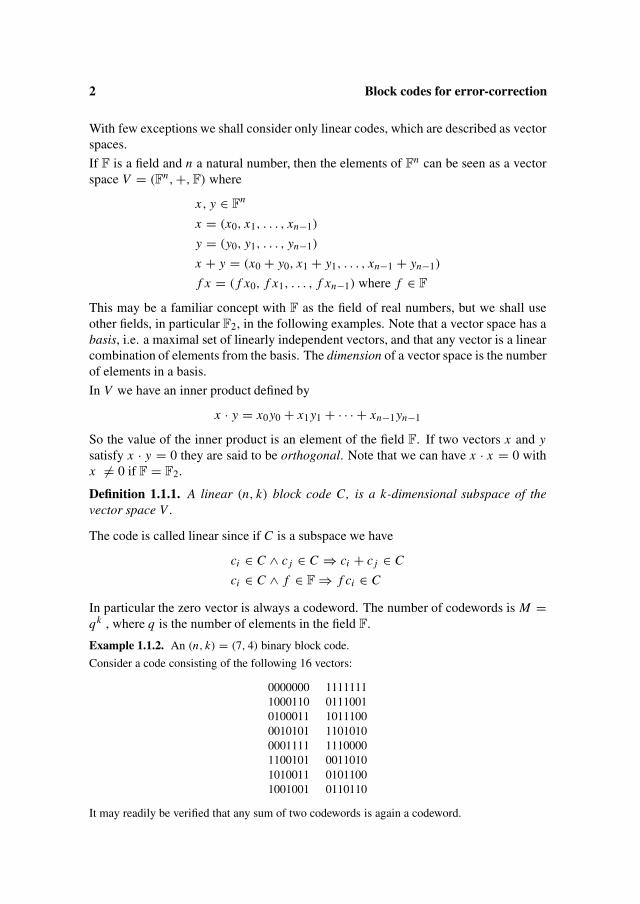
Example 1.1.2. An (n, k) = (7, 4) binary block code.
Consider a code consisting of the following 16 vectors:
0000000 11111111000110 01110010100011 10111000010101 11010100001111 11100001100101 00110101010011 01011001001001 0110110
It may readily be verified that any sum of two codewords is again a codeword.

1.1 Linear codes and vector spaces 3
When a code is used for communication or storage, the information may be assumed tobe a long sequence of binary digits. The sequence is segmented into blocks of lengthk. We may think of such a block of information as a binary vector u of length k. Weshall therefore need an encoding function that maps k-vectors onto codewords. In asystematic encoding, we simply let the first k coordinates be equal to the informationsymbols. The remaining n − k coordinates are sometimes referred to as parity checksymbols and we shall justify this name below.
Instead of listing all the codewords, a code may be specified by a basis of k linearlyindependent codewords.
Definition 1.1.2. A generator matrix G of an (n, k) code C is a k × n matrix whoserows are linearly independent.
If the information is the vector u of length k, we can state the encoding rule as
c = uG (1.1)
Example 1.1.3. A basis for the (7,4) code.
We may select four independent vectors from the list above to give the generator matrix
G =
1 0 0 0 1 1 00 1 0 0 0 1 10 0 1 0 1 0 10 0 0 1 1 1 1
The same code, in the sense of a set of words or a vector space, may be describedby different generator matrices or bases of the vector space. We usually just take onethat is convenient for our purpose. However, G may also be interpreted as specifyinga particular encoding of the information. Thus row operations on the matrix do notchange the code, but the modified G represents a different encoding mapping. SinceG has rank k, we can obtain a convenient form of G by row operations in such a waythat k columns form a k × k identity matrix I . We often assume that this matrix can bechosen as the first k columns and write the generator matrix as
G = (I, A)
This form of the generator matrix gives a systematic encoding of the information.
We may now define a parity check as a vector, h, of length n which satisfies
GhT = 0
where hT denotes the transpose of h.
The parity check vectors are again a subspace of V with dimension n − k.
Definition 1.1.3. A parity check matrix H for an (n, k) code C is an (n −k)×n matrixwhose rows are linearly independent parity checks.
4 Block codes for error-correction
So if G is a generator matrix for the code and H is a parity check matrix, we have
G H T = 0
where 0 is a k × (n − k) matrix of zeroes.
From the systematic form of the generator matrix we may find H as
H = (−AT , I ) (1.2)
where I now is an (n − k) × (n − k) identity matrix. If such a parity check matrix isused, the last n − k elements of the codeword are given as linear combinations of thefirst k elements. This justifies calling the last symbols parity check symbols.
Definition 1.1.4. Let H be a parity check matrix for an (n, k) code C and let r ∈ Fn,then the syndrome s = syn(r ) is given by
s = Hr T (1.3)
We note that if the received word, r = c + e, where c is a codeword and e is the errorpattern (also called the error vector) then
s = H (c + e)T = H eT (1.4)
The term syndrome refers to the fact that s reflects the error in the received word. Thecodeword itself does not contribute to the syndrome, and for an error-free codewords = 0.
It follows from the above definition that the rows of H are orthogonal to the codewordsof C . The code spanned by the rows of H is what is called the dual code C⊥ definedby
C⊥ = {x ∈ Fn|x · c = 0 ∀c ∈ C}It is often convenient to talk about the rate of a code R = k
n . Thus the dual code hasrate 1 − R.
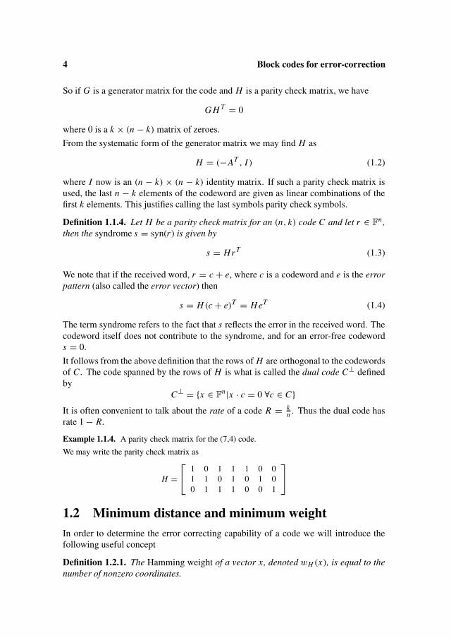
Example 1.1.4. A parity check matrix for the (7,4) code.
We may write the parity check matrix as
H =
1 0 1 1 1 0 01 1 0 1 0 1 00 1 1 1 0 0 1
1.2 Minimum distance and minimum weightIn order to determine the error correcting capability of a code we will introduce thefollowing useful concept
Definition 1.2.1. The Hamming weight of a vector x, denoted wH (x), is equal to thenumber of nonzero coordinates.

1.2 Minimum distance and minimum weight 5
Note that the Hamming weight is often simply called weight.
For a received vector r = c j + e the number of errors is the Hamming weight of e.
We would like to be able to correct all error patterns of weight ≤ t for some t , and wemay use the following definition to explain what we mean by that.
Definition 1.2.2. A code is t-error correcting if for any two codewords ci �= c j , andfor any error patterns e1 and e2 of weight ≤ t , we have ci + e1 �= c j + e2.
This means that it is not possible to get a certain received word from making at most terrors in two different codewords.
A more convenient way of expressing this property uses the notion of Hamming dis-tance
Definition 1.2.3. The Hamming distance between two vectors x and y, denoteddH (x, y) is the number of coordinates where they differ.
It is not hard to see that
dH (x, y) = 0 ⇔ x = y
dH (x, y) = dH (y, x)
dH (x, y) ≤ dH (x, z) + dH (z, y)
So dH satisfies the usual properties of a distance, in particular the third property is thetriangle inequality. With this distance V becomes a metric space.
As with the weight the Hamming distance is often simply called distance, hence wewill in the following often skip the subscript H on the weight and the distance.
Definition 1.2.4. The minimum distance of a code, d, is the minimum Hamming dis-tance between any pair of different codewords.
So the minimum distance can be calculated by comparing all pairs of codewords, butfor linear codes this is not necessary since we have
Lemma 1.2.1. In an (n, k) code the minimum distance is equal to the minimum weightof a nonzero codeword.
Proof. It follows from the definitions that w(x) = d(0, x) and that d(x, y) = w(x − y).Let c be a codeword of minimum weight. Then w(c) = d(0, c) and since 0 is acodeword we have dmin ≤ wmin . On the other hand, if c1 and c2 are codewords atminimum distance, we have d(c1, c2) = w(c1 − c2) and since c1 − c2 is again acodeword we get wmin ≤ dmin . We combine the two inequalities and get the result. �Based on this observation we can now prove
Theorem 1.2.1. An (n, k) code is t-error correcting if and only if t < d2 .

6 Block codes for error-correction
Proof. Suppose t < d2 and we had two codewords ci and c j and two error patterns
e1 and e2 of weight ≤ t such that ci + e1 = c j + e2. Then ci − c j = e2 − e1 butw(e2 − e1) = w(ci − c j ) ≤ 2t < d , contradicting the fact that the minimum weightis d . On the other hand suppose that t ≥ d
2 and let c have weight d . Change t + 1of the nonzero positions to zeroes to obtain y. Then d(0, y) ≤ d − (t + 1) ≤ t andd(c, y) ≤ t but 0 + y = c + (y − c) so the code is not t-error correcting. �
Example 1.2.1. The minimum distance of the (7, 4) code from Example 1.1.2 is 3 and t = 1.
Finding the minimum distance of a code is difficult in general, but the parity checkmatrix can sometimes be used. This is based on the following simple observation.
Lemma 1.2.2. Let C be an (n, k) code and H a parity check matrix for C. Then, if jcolumns are linearly dependent, C contains a codeword with nonzero elements in someof the corresponding positions, and if C contains a word of weight j , then there exist jlinearly dependent columns of H .
This follows directly from the definition of matrix multiplication, since for a codewordc we have H cT = 0.
Lemma 1.2.3. Let C be an (n, k) code with parity check matrix H . The minimumdistance of C equals the minimum number of linearly dependent columns of H .
This follows immediately from the Lemma 1.2.3 and Lemma 1.2.1
For a binary code this means that d ≥ 3 ⇔ the columns of H are distinct and nonzero.
One of our goals is, for given n and k, the construction of codes with large minimumdistance. The following important theorem ensures the existence of certain codes, thesecan serve as a reference for other codes.
Theorem 1.2.2. (The Varshamov-Gilbert bound)
There exists a binary linear code of length n, with at most m linearly independent paritychecks and minimum distance at least d, if
1 +(
n − 1
1
)+ · · · +
(n − 1
d − 2
)< 2m
Proof. We shall construct an m × n matrix such that no d − 1 columns are linearlydependent. The first column can be any nonzero m-tuple. Now suppose we have choseni columns so that no d − 1 are linearly dependent. There are
(i
1
)+ · · · +
(i
d − 2
)
linear combinations of these columns taken d − 2 or fewer at a time. If this numberis smaller than 2m − 1 we can add an extra column such that still d − 1 columns arelinearly independent. �
1.2 Minimum distance and minimum weight 7
For large n, the Gilbert-Varshamov bound indicates that good codes exist, but there isno known practical way of constructing such codes. It is also not known if long binarycodes can have distances greater than indicated by the Gilbert-Varshamov bound. Shortcodes can have better minimum distances. The following examples are particularlyimportant.
Definition 1.2.5. A binary Hamming code is a code whose parity check matrix has allnonzero binary m-vectors as columns.
So the length of a binary Hamming code is 2m − 1 and the dimension is 2m − 1 − m,since it is clear that the parity check matrix has rank m. The minimum distance is atleast 3 by the above and it it easy to see that it is exactly 3. The columns can be orderedin different ways, a convenient method is to represent the natural numbers from 1 to2m − 1 as binary m-tuples.
Example 1.2.2. The (7, 4) code is a binary Hamming code with m = 3.
Definition 1.2.6. An extended binary Hamming code is obtained by adding a zerocolumn to the parity check matrix of a Hamming code and then adding a row of all 1s.
This means that the length of the extended code is 2m . The extra parity check isc0 + c1 + · · · + cn−1 = 0 and therefore all codewords in the extended code have evenweight and the minimum distance is 4. Thus the parameters, (n, k, d), of the binaryextended Hamming code are (2m, 2m − m − 1, 4).
Definition 1.2.7. A biorthogonal code is the dual of the binary extended Hammingcode.
The biorthogonal code has length n = 2m and dimension k = m + 1. It can be seenthat the code consists of the all 0s vector, the all 1s vector and 2n − 2 vectors of weightn2 (See problem 1.5.9).
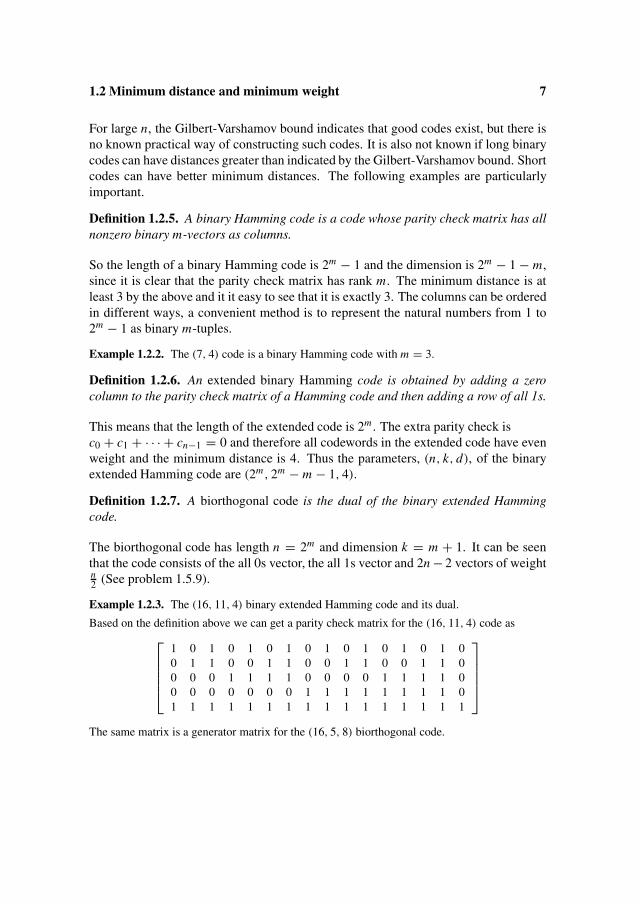
Example 1.2.3. The (16, 11, 4) binary extended Hamming code and its dual.
Based on the definition above we can get a parity check matrix for the (16, 11, 4) code as
1 0 1 0 1 0 1 0 1 0 1 0 1 0 1 00 1 1 0 0 1 1 0 0 1 1 0 0 1 1 00 0 0 1 1 1 1 0 0 0 0 1 1 1 1 00 0 0 0 0 0 0 1 1 1 1 1 1 1 1 01 1 1 1 1 1 1 1 1 1 1 1 1 1 1 1
The same matrix is a generator matrix for the (16, 5, 8) biorthogonal code.

8 Block codes for error-correction
1.3 Syndrome decoding and the Hamming boundWhen a code is used for correcting errors, one of the important problems is the designof a decoder. One can consider this as a mapping from
nFq into the code C, as an
algorithm or sometimes even as a physical device. We will usually see a decoder asa mapping or as an algorithm. One way of stating the objective of the decoder is: fora received vector r , select as the transmitted codeword c a codeword that minimizesd(r, c). This is called maximum likelihood decoding for reasons we will explain inChapter 3. It is clear that if the code is t-error correcting and r = c + e with w(e) ≤ t ,then the output of such a decoder is c.
It is often difficult to design a maximum likelihood decoder, but if we only want tocorrect t errors where t < d
2 it is sometimes easier to get a good algorithm.
Definition 1.3.1. A minimum distance decoder is a decoder that, given a received wordr , selects the codeword c that satisfies d(r, c) < d
2 if such a word exists, and otherwisedeclares failure.
It is obvious that there can be at most one codeword within distance d2 from a received
word.
Using the notion of syndromes from the previous section we can think of a decoder asa mapping of syndromes to error patterns. Thus for each syndrome we should choosean error pattern with the smallest number of errors, and if there are several error pat-terns of equal weight with the same syndrome we may choose one of these arbitrarily.Such a syndrome decoder is not only a useful concept, but may also be a reasonableimplementation if n − k is not too large.
Definition 1.3.2. Let C be an (n, k) code and a ∈ nF . The coset containing a is the
set a + C = {a + c|c ∈ C}.
If two words x and y are in the same coset and H is a parity check matrix of the code,we have H xT = H (a + c1)
T = H aT = H (a + c2)T = H yT so the two words have
the same syndrome. On the other hand if two words x and y have the same syndrome,then H xT = H yT and therefore H (x − y)T = 0, so this is the case if and only if x − yis a codeword and therefore x and y are in the same coset. We therefore have
Lemma 1.3.1. Two words are in the same coset if and only if they have the samesyndrome.
The cosets form a partition of the spacenF into qn−k classes each containing qk ele-
ments.
This gives an alternative way of describing a syndrome decoder: Let r be a receivedword. Find a vector f of smallest weight in the coset containing r (i.e. syn( f ) =syn(r )) and decode into r − f . A word of smallest weight in a coset can be foundonce and for all, such a word is called a coset leader. With a list of syndromes and
1.3 Syndrome decoding and the Hamming bound 9
corresponding coset leaders, syndrome decoding can be performed as follows: Decodeinto r − f where f is the coset leader of the coset corresponding to syn(r ). In thisway we actually do maximum likelihood decoding and can correct qn−k error patterns.If we only list the cosets where the coset leader is unique and have the correspondingsyndromes we do minimum distance decoding.
We illustrate this in
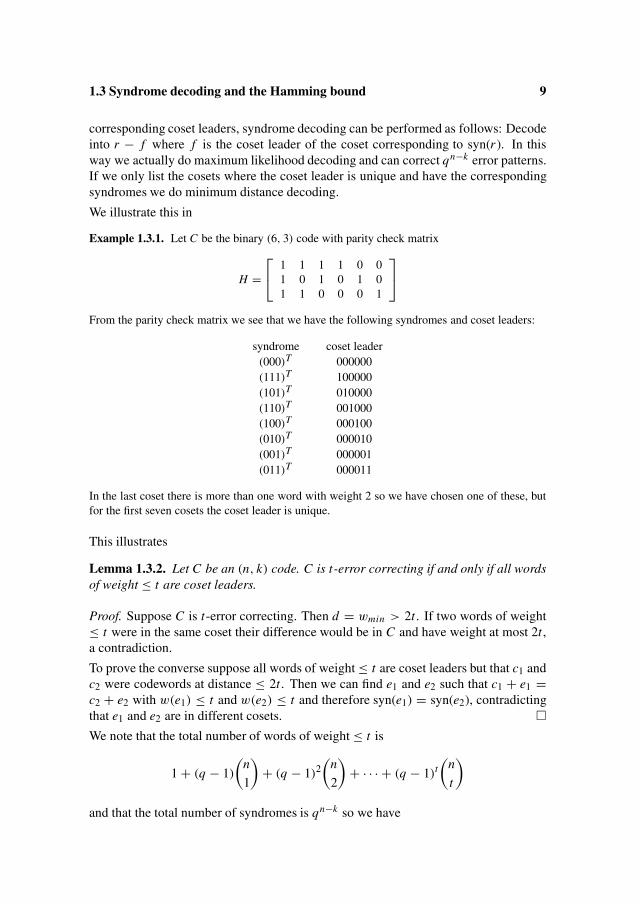
Example 1.3.1. Let C be the binary (6, 3) code with parity check matrix
H =
1 1 1 1 0 01 0 1 0 1 01 1 0 0 0 1
From the parity check matrix we see that we have the following syndromes and coset leaders:
syndrome coset leader(000)T 000000(111)T 100000(101)T 010000(110)T 001000(100)T 000100(010)T 000010(001)T 000001(011)T 000011
In the last coset there is more than one word with weight 2 so we have chosen one of these, butfor the first seven cosets the coset leader is unique.
This illustrates
Lemma 1.3.2. Let C be an (n, k) code. C is t-error correcting if and only if all wordsof weight ≤ t are coset leaders.
Proof. Suppose C is t-error correcting. Then d = wmin > 2t . If two words of weight≤ t were in the same coset their difference would be in C and have weight at most 2t ,a contradiction.
To prove the converse suppose all words of weight ≤ t are coset leaders but that c1 andc2 were codewords at distance ≤ 2t . Then we can find e1 and e2 such that c1 + e1 =c2 + e2 with w(e1) ≤ t and w(e2) ≤ t and therefore syn(e1) = syn(e2), contradictingthat e1 and e2 are in different cosets. �We note that the total number of words of weight ≤ t is
1 + (q − 1)
(n
1
)+ (q − 1)2
(n
2
)+ · · · + (q − 1)t
(n
t
)
and that the total number of syndromes is qn−k so we have
10 Block codes for error-correction
Theorem 1.3.1. (The Hamming bound) If C is an (n, k) code over a field F with qelements that corrects t errors, then
t∑j=0
(q − 1) j(
n
j
)≤ qn−k .
The bound can be seen as an upper bound on the minimum distance of a code withgiven n and k, an upper bound on k if n and d are given or as a lower bound on n if kand d are given.
0 5 10 15 20 25 30 350
20
40
60
80
100
120
140
d
n−k
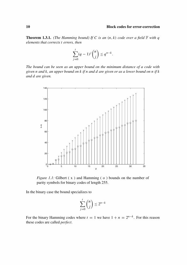
Figure 1.1: Gilbert ( x ) and Hamming ( o ) bounds on the number ofparity symbols for binary codes of length 255.
In the binary case the bound specializes to
t∑j=0
(n
j
)≤ 2n−k
For the binary Hamming codes where t = 1 we have 1 + n = 2n−k . For this reasonthese codes are called perfect.
1.4 Weight distributions 11
1.4 Weight distributionsIf we need more information about the error-correcting capability of a code than whatis indicated by the minimum distance, we can use the weight distribution.
Definition 1.4.1. The weight distribution of a code is a vector A = (A0, A1, . . . , An)
where Aw is the number of codewords of weight w. The weight enumerator is thepolynomial
A(z) =n∑
w=0
Awzw.
We note that for a linear code the number Aw is also the number of codewords ofdistance w from a given codeword. In this sense the geometry of the code as seen froma codeword is the same for all these.
We note an important result on the weight distribution of dual codes
Theorem 1.4.1. (MacWilliams) If A(z) is the weight enumerator of a binary (n, k)
code C, the weight enumerator B(z) of the dual code C⊥ is given by
B(z) = 2−k(1 + z)n A
(1 − z
1 + z
)(1.5)
Because of the importance of the theorem we give a proof even though it is quitelengthy (and may be skipped at first reading).
Proof. Let H be a parity check matrix of C . Let Hext be the matrix that consists of alllinear combinations of the rows of H , so Hext has as rows all the codewords of C⊥.Let y ∈ n
F2 and define the extended syndrome
sext = Hext yT
It is obvious thatc ∈ C ⇔ H cT = 0 ⇔ Hextc
T = sext = 0 (1.6)
Letsext = (s1, s2, . . . s2n−k )
and defineE j = {x ∈ n
F2 |s j = 0}, j = 1, 2, . . . 2n−k
From (1.6) we have that
C = E1 ∩ E2 ∩ · · · ∩ E2n−k
= nF2 \(E1 ∪ E2 ∪ · · · ∪ E2n−k )
whereE j = n
F2 \E j = {x ∈ nF2 |s j = 1}.
12 Block codes for error-correction
If we letE = E1 ∪ · · · ∪ E2n−k
we haveC = n
F2 \E (1.7)
The weight enumerator ofnF2 is
n∑i=0
(n
i
)zi = (1 + z)n,
so if we let E(z) denote the weight enumerator of E we have
A(z) = (1 + z)n − E(z)
In the following we will determine E(z).
We first note that by linearity if sext �= 0, then sext consists of 2n−k−1 0s and 2n−k−1
1s. That means that a word from E is in exactly 2n−k−1 of the E j s and we thereforehave
2n−k−1 E(z) =2n−k∑j=1
E j (z)
where E j (z) is the weight enumerator of E j
Let w j denote the Hamming weight of the j -th row of Hext , then
E j (z) = (1 + z)n−w j
w j∑k=1,odd
(w j
k
)zk
= (1 + z)n−w j1
2
[(1 + z)w j − (1 − z)w j
]
= 1
2(1 + z)n − 1
2(1 + z)n−w j (1 − z)w j
From this we get
E(z) = (1 + z)n − 1
2n−k(1 + z)n
2n−k∑j=1
(1 − z
1 + z
)w j
= (1 + z)n − 1
2n−k(1 + z)n B
(1 − z
1 + z
)(1.8)
and therefore
A(z) = 1
2n−k(1 + z)n B
(1 − z
1 + z
)
By interchanging the roles of C and C⊥ we get the result. �

1.5 Problems 13
From (1.5) we can get
2kn∑
i=0
Bi zi =
n∑w=0
Aw
(1 − z
1 + z
)w
(1 + z)n
2kn∑
i=0
Bi zi =
n∑w=0
Aw(1 − z)w(1 + z)n−w
2kn∑
i=0
Bi zi =
n∑w=0
Aw
w∑m=0
(w
m
)(−z)m
n−w∑l=0
(n − w
l
)zl (1.9)
From which we can find B if A is known and vice versa. The actual calculation can betedious, but can be accomplished by many symbolic mathematical programs.
Example 1.4.1. (Example 1.2.3 continued) The biorthogonal (16, 5, 8) code has weight enu-merator
A(z) = 1 + 30z8 + z16
The weight enumerator for the (16, 11, 4) extended Hamming code can then be found using (1.9)
B(z) = 2−5((1 + z)16 + 30(1 − z)8(1 + z)8 + (1 − z)16
)
= 2−5
16∑j=0
(16
j
)[z j + (−z) j
]+ 30
8∑m=0
(8
m
)(−z)m
8∑l=0
(8
l
)zl
= 1 + 140z4 + 448z6 + 870z8 + 448z10 + 140z12 + z16
1.5 ProblemsProblem 1.5.1 Consider the following binary code
( 0 0 0 0 0 0 )
( 0 0 1 1 1 1 )
( 1 1 0 0 1 1 )
( 1 1 1 1 0 0 )
( 1 0 1 0 1 0 )
1) Is this a linear code?
2) Add more words such that the resulting code is linear.
3) Determine a basis of this code.
Problem 1.5.2 Let C be the binary linear code of length 6 with generator matrix
G =
1 0 1 0 1 01 1 1 1 0 01 1 0 0 1 1

14 Block codes for error-correction
1) Determine a generator matrix for the code of the form (I A).
2) Determine a parity check matrix for the code C⊥.
3) Is (1,1,1,1,1,1) a parity check for the code?
Problem 1.5.3 A linear code has the generator matrix
G =
1 0 0 0 1 1 0 0 1 1 1 00 1 0 0 0 1 1 0 0 1 1 10 0 1 0 0 0 1 1 1 0 1 10 0 0 1 1 0 0 1 1 1 0 1
1) Determine the dimension and the minimum distance of the code and its dual.
2) How many errors do the two codes correct?
Problem 1.5.4 Let the columns of the parity check matrix of a code be h1, h2, h3, h4, h5 so
H =
| | | | |h1 h2 h3 h4 h5| | | | |
1) What syndrome corresponds to an error at position j?
2) Express H(10011)T using h1, h2, h3, h4, h5 .
3) Show that if (1, 1, 1, 1, 1) is a codeword, then h1 + h2 + h3 + h4 + h5 = 0.
Problem 1.5.5 Let C be a code with minimum distance d and parity check matrix H .
1) Show that H has d linearly dependent columns.
2) Show that any d − 1 or fewer columns of H are linearly independent.
3) What is d then?
Problem 1.5.6 Use the Gilbert-Varshamov bound to determine k such that there exists a binary(15, k) code with minimum distance 5.
Problem 1.5.7
1) Determine the parameters of the binary Hamming codes with m = 3, 4, 5 and 8.
2) What are the parameters of the extended codes?
Problem 1.5.8 In Example 1.1.2 we gave a parity check matrix for a Hamming code.
1) What is the dimension and the minimum distance of the dual code?
2) Show that all pairs of codewords in this code have the same distance.
3) Find the minimum distance of the dual to a general binary Hamming code.
These codes are called equidistant because of the property noted in 2).
Problem 1.5.9 Consider the biorthogonal code B(m) of length 2m and dimension m + 1.
1) Show that B(2) contains (0, 0, 0, 0), (1, 1, 1, 1) and six words of weight 2.
2) Show that B(m) contains the all 0s vector, the all 1s vector and 2n − 2 vectors of weight n2 .
3) Replace {0, 1} with {1,−1} in all the codewords and show that these are orthogonal as realvectors.
1.5 Problems 15
Problem 1.5.10 Let G be a generator matrix of an (n, k, d) code C where d ≥ 2. Let G∗ be thematrix obtained by deleting a column of G and let C∗ be the code with generator matrix G∗.
1) What can you say about n∗, k∗ and d∗ ?This process of obtaining a shorter code is called puncturing.Another way of getting a shorter code from an (n, k, d) code C is to force an informationsymbol, x say, to be zero and then delete that position.This process is called shortening.
2) What are the parameters of the shortened code?
Problem 1.5.11 Let H be a parity check matrix for an (n, k) code C . We construct a new codeCext of length n + 1 by defining cn = c0 + c1 + · · · + cn−1.
What can be said about the dimension, the minimum distance and the parity check matrix ofCext ?
Problem 1.5.12 Let C be a binary (n, k) code.
1) Show that the number of codewords that has 0 at position j is either 2k or 2k−1.
2) Show that∑
c∈C w(c) ≤ n · 2k−1 (Hint : Write all the the codewords as rows of a 2k × nmatrix.)
3) Prove that
dmin ≤ n · 2k−1
2k − 1
This is the so-called Plotkin bound.
Problem 1.5.13 Let C be the code with generator matrix
G =
1 0 0 1 0 10 1 0 1 1 10 0 1 0 1 1
1) Determine a parity check matrix for C .
2) Determine the minimum distance of C .
3) Determine the cosets that contain (111111), (110010) and (100000) respectively and find foreach of these the coset leader.
4) Decode the received word (111111).
Problem 1.5.14 Let C be the code of length 9 with parity check matrix
H =
0 1 0 0 1 1 0 0 00 1 1 1 0 0 1 0 01 1 1 1 0 0 0 1 01 1 1 0 1 0 0 0 1
1) What is the dimension of C?
2) Determine the minimum distance of C .
3) Determine coset leaders and the corresponding syndromes for at least 11 cosets.
4) Is 000110011 a codeword?
5) Decode the received words 110101101 and 111111111.

16 Block codes for error-correction
Problem 1.5.15 Let C be an (n, k) code with minimum distance 5 and parity check matrix H .
Is it true that H(1110 . . . 0)T = H(001110 . . . 0)T ?
Problem 1.5.16 Determine a parity check matrix for a code that has the following coset leaders:000000, 100000, 010000, 001000, 000100, 000010, 000001, 110000.
Problem 1.5.17 Find an upper bound on k for which there exists a (15, k) code with minimumdistance 5. Compare the result with Problem 1.5.6
Problem 1.5.18 An (8, 1) code consists of the all 0s word and the all 1s word.
What is the weight distribution of the dual code?
Problem 1.5.19 In this problem we investigate the existence of a binary (31, 22, 5) code C .
1) Show that the Hamming bound does not rule out the existence of such a code.
2) Determine the number of cosets of C and determine the number of coset leaders of weight0, 1, and 2 respectively.
3) Determine for each of the cosets, where the coset leaders have weights 0, 1 or 2, the maximalnumber of words of weight 3 in such a coset.
4) Determine for each of the cosets, where the coset leader has weight at least 3, the maximalnumber of words of weight 3 in such a coset.
5) Show that this leads to a contradiction and therefore that such a code does not exist!
Problem 1.5.20 Let C be the binary (32, 16) code with generator matrix G = (I, A) where I isa 16 × 16 identity matrix and
A =
J I I II J I II I J II I I J
where I is a 4 × 4 identity matrix and
J =
1 1 1 11 1 1 11 1 1 11 1 1 1
1) Prove that C = C⊥ i.e. the code is self dual. (Why is it enough to show that each row in G isorthogonal to any other row?)
2) Determine a parity check matrix H .
3) Find another generator matrix of the form G′ = (A′, I )
4) Prove that for a self dual code the following statement is true: If two codewords both haveweights that are multiples of 4, that is also true for their sum.
5) Prove that the minimum distance of the code is a multiple of 4.
6) Prove that the minimum distance is 8.
7) How many errors can the code correct?
8) How many cosets does the code have?
9) How many error patterns are there of weight 0, 1, 2 and 3?
10) How many cosets have coset leaders of weight at least 4?

1.5 Problems 17
Problem 1.5.21 Project Write a program for decoding the (32, 16) code above using syndromedecoding. If more than three errors occur, the program should indicate a decoding failure andleave the received word unchanged.
We suggest that you generate a table of error patterns using the syndrome as the address. Initiallythe table is filled with the all 1s vector (or some other symbol indicating decoding failure). Thenthe syndromes for zero to three errors are calculated, and the error patterns are stored in thecorresponding locations.
Assume that the bit error probability is 0.01.
1) What is the probability of a decoding failure?
2) Give an estimate of the probability of decoding to a wrong codeword.
Problem 1.5.22 Project Write a program that enables you to determine the weight enumeratorof the binary (32, 16) code above.
One way of getting all the codewords is to let the information vector run through the 216 possi-bilities by converting the integers from 0 to 216 − 1 to 16 bit vectors and multiply these on thegenerator matrix.
Problem 1.5.23 Project A way to construct binary codes of prescribed length n and minimumdistance d is the following: List all the binary n vectors in some order and choose the codewordsone at the time such that it has distance at least d from the previously chosen words. Thisconstruction is greedy in the sense that it selects the first vector on a list that satisfies the distancetest. Clearly different ways of listing all length n binary vectors will produce different codes.One such list can be obtained by converting the integers from 0 to 2n − 1 to binary n vectors.
Write a program for this greedy method.
1) Try distance 3, 5 and 6. Do you get good codes?
2) Are the codes linear? If so why?
You might try listing the binary vectors in a different order.


Chapter 2
Finite fields
As we have stated earlier we shall consider codes where the alphabet is a finite field.In this chapter we define finite fields and investigate some of the most important prop-erties. We have chosen to cover in the text only what we think is necessary for codingtheory. Some additional material is treated in the problems.
2.1 Fundamental properties of finite fields
We begin with the definition of a field.
Definition 2.1.1. A field F is a nonempty set, S, with two binary operations, + and ·,and two different elements of S, 0 and 1, such that the following axioms are satisfied.
1. ∀x, y x + y = y + x
2. ∀x, y, z (x + y) + z = x + (y + z)
3. ∀x x + 0 = x
4. ∀x ∃(−x) x + (−x) = 0
5. ∀x, y x · y = y · x
6. ∀x, y, z x · (y · z) = (x · y) · z
7. ∀x x · 1 = x
8. ∀x �= 0 ∃x−1 x · x−1 = 1
9. ∀x, y, z x · (y + z) = x · y + x · z
Classical examples of fields are the rational numbers Q, the real numbers R, and thecomplex numbers C.
20 Finite fields
If the number of elements, |S|, in S is finite we have a finite field and it is an interestingfact that these can be completely determined in the sense that these exist if and only ifthe number of elements is a power of a prime and they are essentially unique. In thefollowing we will consider only the case where |S| = p, p is a prime, and |S| = 2m .
Theorem 2.1.1. Let p be a prime and let S = {0, 1, . . . , p − 1}. Let + and · denoteaddition and multiplication modulo p respectively. Then (S,+, ·, 0, 1) is a finite fieldwith p elements which we denote Fp.
Proof. It follows from elementary number theory that the axioms 1 – 7 and 9 are sat-isfied. That the nonzero elements of S have a multiplicative inverse (axiom 8) can beseen in the following way:
Let x be a nonzero element of S and consider the set S = {1 · x, 2 · x, . . . , (p − 1) · x}.We will prove that the elements in S are different and nonzero so therefore S = S\{0}and in particular there exists an i such that i · x = 1.
It is clear that 0 /∈ S since 0 = i · x, 1 ≤ i ≤ p − 1 implies p|i x and since p is a primetherefore p|i or p|x , a contradiction.
To see that the elements in S are different suppose that i · x = j · x where 1 ≤ i, j ≤p − 1. We then get p|(i x − j x) ⇔ p|(i − j)x and again since p is a prime we getp|(i − j) or p|x . But x < p and i − j ∈ {−(p−2), . . . , (p−2)} so therefore i = j . �
Example 2.1.1. The finite field F2
If we let p = 2, we get F2 that we have already seen.
Example 2.1.2. The finite field F3.
If we let p = 3 we get the ternary field with elements 0, 1, 2.
In that we have
0 + 0 = 0, 0 + 1 = 1 + 0 = 1, 0 + 2 = 2 + 0 = 2, 1 + 1 = 2,
1 + 2 = 2 + 1 = 0, 2 + 2 = 1, 0 · 0 = 0 · 1 = 1 · 0 = 2 · 0 = 0 · 2 = 0,
1 · 2 = 2 · 1 = 2, 2 · 2 = 1, (so 2−1 = 2 !)
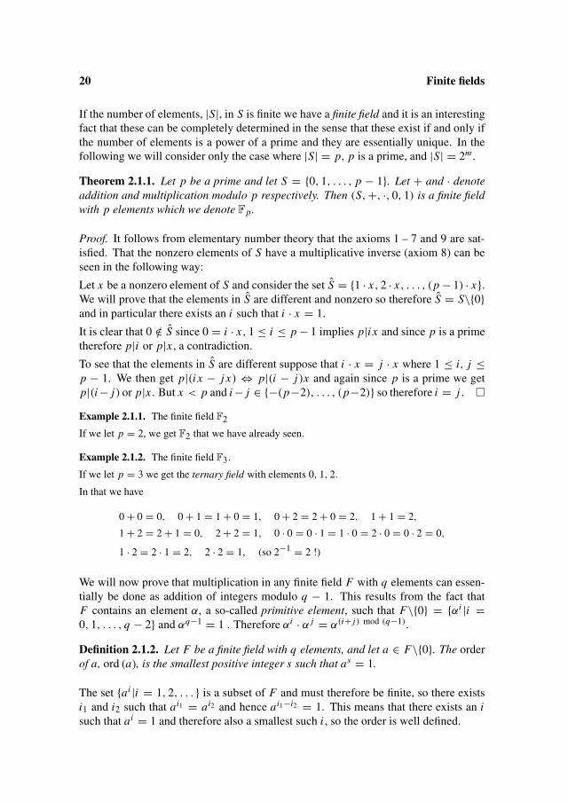
We will now prove that multiplication in any finite field F with q elements can essen-tially be done as addition of integers modulo q − 1. This results from the fact thatF contains an element α, a so-called primitive element, such that F\{0} = {αi |i =0, 1, . . . , q − 2} and αq−1 = 1 . Therefore αi · α j = α(i+ j ) mod (q−1).
Definition 2.1.2. Let F be a finite field with q elements, and let a ∈ F\{0}. The orderof a, ord (a), is the smallest positive integer s such that as = 1.
The set {ai |i = 1, 2, . . . } is a subset of F and must therefore be finite, so there existsi1 and i2 such that ai1 = ai2 and hence ai1−i2 = 1. This means that there exists an isuch that ai = 1 and therefore also a smallest such i , so the order is well defined.

2.1 Fundamental properties of finite fields 21
Lemma 2.1.1. Let F be a finite field with q elements, and let a, b ∈ F\{0}; then
1. ord (a) = s ⇒ a, a2, . . . , as are all different.
2. a j = 1 ⇔ ord (a) | j .
3. ord(a j) = ord(a)
gcd(ord(a), j ) .
4. ord (a) = s, ord (b) = j , gcd(s, j) = 1 ⇒ ord (ab) = s j .
Proof.
1. If ai = a j , 0 < i < j ≤ s we get a j−i = 1 with 0 < j − i < s, contradictingthe definition of order.
2. If ord (a) = s and j = sh we get a j = ash = (as)h = 1. If a j = 1 we letj = sh + r with 0 ≤ r < s and get 1 = a j = ash+r = (as)har = ar andtherefore r = 0 by the definition of order, so s| j .
3. Let ord (a) = s and ord(a j) = l; then 1 = (a j )l = a jl so by 2, we get s| j l and
therefore sgcd(s, j )
∣∣ j lgcd(s, j ) hence s
gcd(s, j )
∣∣l.
On the other hand (a j )s
gcd( j,s) = (as)j
gcd( j,s) = 1 so again by 2 we have l∣∣ s
gcd( j,s)and therefore l = s
gcd( j,s) .
4. (ab)s j = (as) j (b j )s = 1 · 1 = 1 so by 2 ord (ab) |s j , but since gcd(s, j) = 1this means that ord (ab) = l1 · l2 where l1|s and l2| j .
So 1 = (ab)l1l2 and therefore 1 = [(ab)l1l2 ] sl1 = asl2bsl2 = bsl2 so by 2 j |l2s
and since gcd( j, s) = 1 we have j |l2 and hence j = l2.
In the same way we get s = l1 and the claim is proved. �
The lemma enables us to prove
Theorem 2.1.2. Let F be a finite field with q elements, then F has an element of orderq − 1.
Proof. Since |F\{0}| = q − 1 it follows from 1 of Lemma 2.1.1 that the order of anyelement is at most q − 1.
Let α be an element of maximal order and β any element in F\0.
Let ord (α) = r and ord (β) = s. We will first show that s|r .
Suppose not, then there exists a prime p and natural numbers i and j such that r =pi · a, s = p j · b with j > i and gcd(a, p) = gcd(b, p) = 1.
We have from Lemma 2.1.1 3 that
ord(α pi
)= r
gcd(r, pi
) = a and ord(βb)
= s
gcd(s, b)= p j

22 Finite fields
and since gcd(a, p) = 1 we get from 2.1.1 4
ord(α pi · βb
)= a · p j > a · pi = r
contradicting the assumption that r is the maximal order.
So we have ord (β) |ord (α).
This implies that every element of F\{0} is a zero of the polynomial zord(α) − 1 andsince a polynomial of degree n can have at most n zeroes (see Theorem 2.2.2) weconclude that ord (α) ≥ q − 1 and hence that ord (α) = q − 1 and the theorem isproved. �
Corollary 2.1.1. The order of any nonzero element in a finite field with q elementsdivides q − 1.
Corollary 2.1.2. Any element γ of a finite field with q elements satisfies γ q − γ = 0.
The theorem does not give a method to find a primitive element; usually one has to usetrial and error.
Example 2.1.3. 3 is a primitive element of F17.
Since the possible orders of a nonzero element of F17 are 1, 2, 4, 8 and 16 but 32 = 9, 34 = 13and 38 = 16 we see that 3 must have order 16.
2.2 The finite field F2m
In the following we will consider some of the properties of polynomials with coeffi-cients in a field and present the construction of a finite field with 2m elements.
Recall that if F is a field, then F[x] denotes the set of polynomials with coefficientsfrom F , i.e. expressions of the form
anxn + · · · + a1x + a0
where ai ∈ F . We have the notion of the degree of a polynomial (denoted deg) and cando addition and multiplication of polynomials.
Theorem 2.2.1. Let a(x), b(x) ∈ F[x], b(x) �= 0; then there exist unique polynomialsq(x) and r(x) with deg (r(x)) < deg(b(x)) such that
a(x) = q(x)b(x) + r(x)
Proof. To prove the uniqueness suppose a(x) = q1(x)b(x) + r1(x) and a(x) =q2(x)b(x) + r2(x) where deg(r1(x)) < deg(b(x)) and deg(r2(x)) < deg(b(x)). Wethen get r2(x) − r1(x) = b(x)(q1(x) − q2(x)), but since the degree of the polyno-mial on the left hand- side is smaller than the degree of b(x), this is only possible if(q1(x) − q2(x)) = 0 and r2(x) − r1(x) = 0.

2.2 The finite field F2m 23
To prove the existence we first note that if deg(b(x)) > deg(a(x)) we have a(x) =0 · b(x) + a(x) so the claim is obvious here. If deg(b(x)) ≤ deg(a(x)) let a(x) =anxn + · · · + a1x + a0 and b(x) = bm xm + · · · + b1x + b0 and look at the polynomialb−1
m anxn−mb(x) − a(x). This has degree < n so we can use induction on the degree ofa(x) to get the result. �
Theorem 2.2.2. A polynomial of degree n has at most n zeroes.
Proof. Let a be a zero of the polynomial f (x) ∈ F[x]. By the above we have thatf (x) = q(x)(x − a) + r(x) with deg(r(x)) < 1 so r(x) must be a constant. Since a isa zero of f (x) we have 0 = f (a) = q(a) · 0 + r(a) and therefore r(x) = r(a) = 0 sof (x) = q(x)(x − a) and q(x) has degree n − 1. If b, b �= a also is a zero of f (x), itmust be a zero of q(x) so we can repeat the argument and eventually get the result. �A polynomial f (x) ∈ F[x] is called irreducible if f (x) = a(x)b(x) implies thatdeg(a(x)) = 0 or deg(b(x)) = 0 (e.g. either a(x) or b(x) is a constant).
Irreducible polynomials play the same role in F[x] as prime numbers for the integers,since it can be shown that any polynomial can be written (uniquely) as a product of irre-ducible polynomials. From this follows that if f (x) is irreducible and f (x)|a(x)b(x),then f (x)|a(x) or f (x)|b(x). Actually the proofs are fairly easy modifications of thecorresponding proofs for the integers.
Example 2.2.1. Irreducible polynomials from F2[x] of degree at most 4
These are: Of degree 1: x , x + 1. Irreducible polynomials of higher degree must have constantterm 1 since else x would be a factor and an odd number of terms since else 1 would be a zeroand therefore (x −1) would be a factor, so of degrees 2 and 3 we get: x2 + x +1, x3 + x +1 andx3 + x2 +1. Of degree 4 we get: x4 + x +1, x4 + x3 +1, x4 + x3 + x2 + x +1. The polynomialx4 + x2 + 1 which also has an odd number of terms and constant term 1 is not irreducible sincex4 + x2 + 1 = (x2 + x + 1)2.
We are now ready to construct the field F2m .
As elements of F2m we take the 2m m-tuples with elements from F2 and addition isdefined coordinatewise. This implies that a + a = 0. It is easy to see that the first fouraxioms for a field are satisfied.
Multiplication is somewhat more complicated. Let f (x) ∈ F2[x] be an irreduciblepolynomial of degree m. Let a = (a0, a1, . . . , am−1) and b = (b0, b1, . . . , bm−1) andtherefore a(x) = am−1xm−1+· · ·+a1x+a0 and b(x) = bm−1xm−1+· · ·+b1x+b0 . Wedefine the multiplication as a(x)b(x) modulo f (x), i.e. if a(x)b(x) = q(x) f (x)+r(x)
where deg(r(x)) < m, we set r = (r0, r1, . . . , rm−1). If we let 1 = (1, 0, . . . , 0) wesee that 1 · a = a.
With the addition and multiplication we have just defined we have constructed a field.This is fairly easy to see, again the most difficult part is to prove the existence of amultiplicative inverse for the nonzero elements.
To this end we copy the idea from Fp . Let a ∈ F2m \{0}. The set A = {a · h|h ∈F2m \{0}} does not contain 0 since this would, for the corresponding polynomials, imply

24 Finite fields
that f (x)|a(x) or f (x)|h(x). Moreover the elements of A are different since if a ·h1 =a · h2 we get for the corresponding polynomials that f (x)|a(x)(h1(x) − h2(x)), andsince f (x) is irreducible this implies f (x)|a(x) or f (x)|h1(x)−h2(x). But this is onlypossible if h1(x) = h2(x), since f (x) has degree m but both a(x) and h1(x) − h2(x)
have degree < m. This gives that A = F2m \{0} and in particular that 1 ∈ A.
It can be proven that for any positive integer m there exists an irreducible polynomialof degree m with coefficients in F2 and therefore the above construction gives for anypositive integer m a finite field with q = 2m elements; we denote this Fq . It can alsobe proven that essentially Fq is unique.
Example 2.2.2. The the finite field F4
Let the elements be 00, 10, 01 and 11, then we get the following table for the addition:
+ 00 10 01 1100 00 10 01 1110 10 00 11 0101 01 11 00 1011 11 01 10 00
Using the irreducible polynomial x2 + x + 1 we get the following table for multiplication:
· 00 10 01 1100 00 00 00 0010 00 10 01 1101 00 01 11 1011 00 11 10 01
From the multiplication table it is seen that the element 01 corresponding to the polynomial x isprimitive, i.e. has order 3.
We have seen that multiplication in a finite field is easy once we have a primitiveelement and from the construction above addition is easy when we have the elementsas binary m-tuples. Therefore we should have a table listing all the binary m-tuples andthe corresponding powers of a primitive element in order to do calculations in F2m . Weillustrate this in
Example 2.2.3. The finite field F16
The polynomial x4 + x + 1 ∈ F2[x] is irreducible and can therefore be used to construct F16.The elements are the binary 4-tuples : (0, 0, 0, 0) . . . (1, 1, 1, 1). These can also be consideredas all binary polynomials of degree at most 3. If we calculate the powers of (0, 1, 0, 0) whichcorresponds to the polynomial x we get:
x0 = 1 , x1 = x , x2 = x2, x3 = x3, x4 = x + 1, x5 = x2 + x , x6 = x3 + x2, x7 = x3 + x + 1,x8 = x2 + 1, x9 = x3 + x , x10 = x2 + x + 1, x11 = x3 + x2 + x , x12 = x3 + x2 + x + 1,x13 = x3 + x2 + 1, x14 = x3 + 1, x15 = 1.
2.3 Minimal polynomials and factorization of xn − 1 25
This means we can use (0, 1, 0, 0) as a primitive element which we call α and list all the binary4-tuples and the corresponding powers of α.
binary 4 − tuple power of α polynomial0000 00001 α0 10010 α x0100 α2 x2
1000 α3 x3
0011 α4 x + 10110 α5 x2 + x1100 α6 x3 + x2
1011 α7 x3 + x + 10101 α8 x2 + 11010 α9 x3 + x0111 α10 x2 + x + 11110 α11 x3 + x2 + x1111 α12 x3 + x2 + x + 11101 α13 x3 + x2 + 11001 α14 x3 + 1
If f (x) ∈ F2[x] is irreducible and has degree m it can be used to construct F2m as wehave seen. If we do this, then there exists an element β ∈ F2m such that f (β) = 0,namely the element corresponding to the polynomial x . This follows directly from theway F2m is constructed.
Actually as we shall see the polynomial f (x) can be written as a product of polynomi-als from F2m [x] of degree 1.
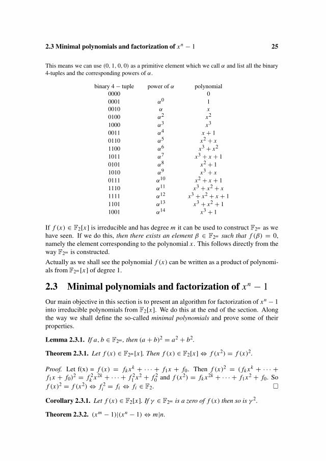
2.3 Minimal polynomials and factorization of xn − 1
Our main objective in this section is to present an algorithm for factorization of xn − 1into irreducible polynomials from F2[x]. We do this at the end of the section. Alongthe way we shall define the so-called minimal polynomials and prove some of theirproperties.
Lemma 2.3.1. If a, b ∈ F2m , then (a + b)2 = a2 + b2.
Theorem 2.3.1. Let f (x) ∈ F2m [x]. Then f (x) ∈ F2[x] ⇔ f (x2) = f (x)2.
Proof. Let f(x) = f (x) = fk xk + · · · + f1x + f0. Then f (x)2 = ( fk xk + · · · +f1x + f0)
2 = f 2k x2k + · · · + f 2
1 x2 + f 20 and f (x2) = fk x2k + · · · + f1x2 + f0. So
f (x)2 = f (x2) ⇔ f 2i = fi ⇔ fi ∈ F2. �
Corollary 2.3.1. Let f (x) ∈ F2[x]. If γ ∈ F2m is a zero of f (x) then so is γ 2.
Theorem 2.3.2. (xm − 1)|(xn − 1) ⇔ m|n.

26 Finite fields
Proof. Follows from the identity:
xn − 1 = (xm − 1)(xn−m + xn−2m + · · · + xn−km) + xn−km − 1 �
Theorem 2.3.3. F2m is a subfield of F2n ⇔ m|n.
Proof. If F2m is a subfield of F2n , then F2n contains an element of order 2m − 1and therefore (2m − 1)|(2n − 1) and so m|n. If m|n we have (2m − 1)|(2n − 1) andtherefore(x2m−1 − 1)|(x2n−1 − 1) so (x2m − x)|(x2n − x) and hence F2m = {x |x2m =x} ⊂ F2n = {x |x2n = x}. �
Definition 2.3.1. Let γ be an element of F2m . The minimal polynomial of γ , mγ (x) isthe polynomial in F2[x] of lowest degree that has γ as a zero.
Since γ is a zero of x2m − x indeed there exists a binary polynomial with γ as a zero.The minimal polynomial is unique since if there were two of the same degree theirdifference would have lower degree but still have γ as a zero.
Theorem 2.3.4. Let γ be an element of F2m and let mγ (x) ∈ F2[x] be the minimalpolynomial of γ . Then:
1. mγ (x) is irreducible.
2. If f (x) ∈ F2[x] satisfy f (γ ) = 0, then mγ (x)| f (x).
3. x2m − x is the product of the different minimal polynomials of the elements ofF2m .
4. deg(mγ (x)) ≤ m, with equality if γ is a primitive element.
Proof.
1. If mγ (x) = a(x)b(x) we would have a(γ ) = 0 or b(γ ) = 0, contradicting theminimality of the degree of mγ (x).
2. Let f (x) = mγ (x)q(x)+r(x) with deg(r(x)) < deg(mγ (x)). This gives r(γ ) =0 and therefore r(x) = 0.
3. Any element of F2m is a zero of x2m − x , so by 2 we get the result.
4. Since F2m can be seen as a vector space over F2 of dimension m, the m + 1elements, 1, γ , . . . , γ m , are linearly dependent so there exists (a0, a1, . . . , am),ai ∈ F2 such that amγ m + · · · + a1γ + a0 = 0. If γ is a primitive element1, γ , . . . , γ m−1 must be linearly independent, since if not, the powers of γ wouldgive fewer than 2m − 1 different elements. �
Theorem 2.3.5. x2m − x = the product of all binary irreducible polynomials whosedegrees divide m.

2.3 Minimal polynomials and factorization of xn − 1 27
Proof. Let f (x) be an irreducible polynomial of degree d where d|m. We want toprove that f (x)|x2m − x . This is trivial if f (x) = x so we assume f (x) �= x . Sincef (x) is irreducible it can be used to construct F2d and f (x) is the minimal polynomial
of some element in F2d ; so by 2, above, we have f (x)|x2d−1 − 1 and since d|m wehave from that 2d −1|2m −1 and therefore x2d−1 −1|x2m−1 −1. Conversely if f (x) isirreducible, divides x2m − x and has degree d , we shall prove that d|m. Again we canassume f (x) �= x and hence f (x)|x2m−1 − 1. We can use f (x) to construct F2d . Letβ ∈ F2d be a zero of f (x) and let α be a primitive element of F2d , say
α = ad−1βd−1 + · · · + a1β + a0 (2.1)
Since f (β) = 0 we have β2m = β and by equation (2.1) and Lemma 2.3.1 thereforeα2m = α and hence α2m−1 = 1. Then the order 2d − 1 of α must divide 2m − 1 so byTheorem 2.3.2 d|m and we are finished. �
Definition 2.3.2. Let n be an odd number and let j be an integer 0 ≤ j < n. Thecyclotomic coset containing j is defined as
{ j, 2 j mod n, . . . , 2i j mod n, . . . , 2s−1 j mod n}where s is the smallest positive integer such that 2s j mod n = j .
If we look at the numbers, 2i j mod n, i = 0, 1, . . . , they can not all be different soindeed the s in the definition above exists.
If n = 15 we get the following cyclotomic cosets:
{0}{1, 2, 4, 8}{3, 6, 12, 9}
{5, 10}{7, 14, 13, 11}
We will use the notation that if j is the smallest number in a cyclotomic coset, thenthat coset is called C j . The subscripts j are called coset representatives. So the abovecosets are C0, C1, C3, C5 and C7. Of course we always have C0 = {0}.It can be seen from the definition that if n = 2m − 1 and we represent a number i as abinary m-vector, then the cyclotomic coset containing i consists of that m-vector andall its cyclic shifts.
The following algorithm is based on
Theorem 2.3.6. Suppose n is an odd number, and that the cyclotomic coset C1 has
m elements. Let α be a primitive element of F2m and β = α2m −1
n . Then mβ j =∏i∈c j
(x − β i ).

28 Finite fields
Proof. Let f j = ∏i∈c j
(x − β i ), then f j (x2) = ( f j (x))2 by Definition 2.3.2 and thefact that β has order n. It then follows from Theorem 2.3.1 that f j (x)F2[x].We also have that f j (β
j ) = 0 so mβ j | f j (x) by Theorem 2.3.4. It follows from Corol-
lary 2.3.1 that the elements(β j)i
with i ∈ C j also are zeroes of mβ j (x) and thereforemβ j = f j (x). �
Corollary 2.3.2. With notation as above we have
xn − 1 =∏
j
f j (x)
We can then give the algorithm. Since this is the first time we present an algorithm, weemphasize that we use the concept of an algorithm in the common informal sense of acomputational procedure, which can be effectively executed by a person or a suitableprogrammed computer. There is abundant evidence that computable functions do notdepend on the choice of a specific finite set of basic instructions or on the programminglanguage. An algorithm takes a finite input, and terminates after a finite number of stepsproducing a finite output. In some cases no output may be produced, or equivalently aparticular message is generated. Some programs do not terminate on certain inputs, butwe exclude these from the concept of an algorithm. Here, algorithms are presented instandard algebraic notation, and it should be clear from the context that the descriptionscan be converted to programs in a specific language.
Algorithm 2.3.1. Factorization of xn − 1
Input: An odd number n
1. Find the cyclotomic cosets modulo n.
2. Find the number m of elements in C1.
3. Construct the finite field F2m , select a primitive element α and put β = α2m −1
n .
4. Calculatef j (x) =
∏i∈c j
(x − β i ), j = 0, 1, . . . .
Output: The factors of xn − 1, f0(x), f1(x), . . .
One can argue that this is not really an algorithm because in step 3 one needs an irre-ducible polynomial in F2[x] of degree m.
The table in appendix C not only gives such polynomials up to degree 16, these arealso chosen such that they are minimal polynomials of a primitive element.
For m ≤ 8 we have moreover given the minimal polynomials for α j , where j is a cosetrepresentative.

2.4 Problems 29
Example 2.3.1. Factorization of x51 − 1
The cyclotomic cosets modulo 51 are
C0 = {0}C1 = {1, 2, 4, 8, 16, 32, 13, 26}C3 = {3, 6, 12, 24, 48, 45, 39, 27}C5 = {5, 10, 20, 40, 29, 7, 14, 28}C9 = {9, 18, 36, 21, 42, 33, 15, 30}
C11 = {11, 22, 44, 37, 23, 46, 41, 31}C17 = {17, 34}C19 = {19, 38, 25, 50, 49, 47, 43, 35}
We see that |C1| = 8. Since 28−151 = 5 we have that β = α5 where α is a primitive element
of F28 .
Using the table from Appendix C (the section with m = 8) we get for the minimal polynomials:
m1(x) = 1 + x
mβ(x) = mα5(x) = x8 + x7 + x6 + x5 + x4 + x + 1
mβ3 (x) = mα15(x) = x8 + x7 + x6 + x4 + x2 + x + 1
mβ5 (x) = mα25(x) = x8 + x4 + x3 + x + 1
mβ9 (x) = mα45(x) = x8 + x5 + x4 + x3 + 1
mβ11 (x) = mα55(x) = x8 + x7 + x5 + x4 + 1
mβ17 (x) = mα85(x) = x2 + x + 1
mβ19 (x) = mα95(x) = x8 + x7 + x4 + x3 + x2 + x + 1
2.4 Problems
Problem 2.4.1 In this problem we are considering F17.
1) What is the sum of all the elements?
2) What is the product of the nonzero elements?
3) What is the order of 2?
4) What are the possible orders of the elements?
5) Determine for all the possible orders an element of that order.
6) How many primitive elements are there?.
7) Try to solve the equation x2 + x + 1 = 0.
8) Try to solve the equation x2 + x − 6 = 0.

30 Finite fields
Problem 2.4.2 Let F be a field.
1) Show that a · b = 0 ⇒ a = 0 or b = 0.
2) Show that {0, 1, 2, 3} with addition and multiplication modulo 4 is not a field.
Problem 2.4.3 Let a ∈ Fq . Determine
q−2∑j=0
(ai ) j
Problem 2.4.4 Determine all binary irreducible polynomials of degree 3.
Problem 2.4.5 Construct F8 using f (x) = x3 + x + 1 , that is explain what the elements areand how to add and multiply them.
Construct a multiplication table for the elements of F8�{0, 1}.Problem 2.4.6 Which of the following polynomials can be used to construct F16?
x4 + x2 + x, x4 + x3 + x2 + 1, x4 + x + 1, x4 + x2 + 1.
Problem 2.4.7 We consider F16 as constructed in Example 2.2.3
1) Determine the sum of all the elements of F16.
2) Determine the product of all the nonzero elements of F16.
3) Determine all the primitive elements of F16.
Problem 2.4.8
1) The polynomial z4 + z3 + 1 has zeroes in F16. How many?
2) The polynomial z4 + z2 + z has zeroes in F16. How many?
Problem 2.4.9 Let f (x) = (x2 + x + 1)(x3 + x + 1).
Determine the smallest number m such that f (x) has five zeroes in F2m .
Problem 2.4.10 What are the possible orders of the elements in F25? and in F26 ?
Problem 2.4.11 Factorize x9 − 1 over F2.
Problem 2.4.12 Factorize x73 − 1 over F2.
Problem 2.4.13 Factorize x85 − 1 over F2.
Problem 2.4.14 Factorize x18 − 1 over F2.
Problem 2.4.15 Is x8 + x7 + x6 + x5 + x4 + x + 1 an irreducible polynomial over F2 ?
Problem 2.4.16
1) Show that f (x) = x4 + x3 + x2 + x + 1 is irreducible in F2[x].2) Construct F16 using f (x) , that is explain what the elements are and how to add and multiply
them.
3) Determine a primitive element.
4) Show that the polynomial z4 + z3 + z2 + z + 1 has four roots in F16.

2.4 Problems 31
Problem 2.4.17 Let f (x) ∈ F2[x] be an irreducible polynomial of degree m. Then f (x) has azero γ in F2m .
By solving 1) – 7) below you shall prove the following: f (x) has m different zeroes in F2m andthese have the same order.
1) Show that f (γ 2) = f (γ 4) = · · · = f (γ 2m−1) = 0.
2) Show that γ, γ 2, . . . , γ 2m−1have the same order.
3) Show that γ 2i = γ 2 j, j > i ⇒ γ 2 j−i = γ . (You can use the fact that a2 = b2 ⇒ a = b)
Let s be the smallest positive number such that γ 2s = γ .
4) Show that γ, γ 2, . . . , γ 2s−1are different.
5) Show that g(x) = (x − γ )(x − γ 2) · · · (x − γ 2s−1) divides f (x).
6) Show that g(x) ∈ F2[x].7) Show that g(x) = f (x) and hence s = m.
Problem 2.4.18
1) Determine the number of primitive elements of F32.
2) Show that the polynomial x5 + x2 + 1 is irreducible over F2.
3) Are there elements γ in F32 that has order 15?
4) Is F16 a subfield of F32?
We construct F32 using the polynomial x5 + x2 + 1. Let α be an element of F32 that satisfiesα5 + α2 + 1 = 0.
5) What is (x − α)(x − α2)(x − α4)(x − α8)(x − α16)?
6) α4 + α3 + α = αi . What is i?
F32 can be seen as a vector space over F2.
7) Show that the dimension of this vector space is 5.
Let γ be an element of F32, γ �= 0, 1.
8) Show that γ is not a root of a binary polynomial of degree less than 5.
9) Show that 1, γ , γ 2, γ 3, γ 4 is a basis for the vector space.
10) What are the coordinates of α8 with respect to the basis 1, α, α2, α3, α4?
Problem 2.4.19 Let C be a linear (n, k, d) code over Fq .
1) Show that d equals minimal number of linearly dependent columns of a parity matrix H .
2) What is the maximal length of an (n, k, 3) code over Fq?
3) Construct a maximal length (n, k, 3) code over Fq and show that it is perfect, i.e. that a1 + (q − 1)n = qn−k .

Chapter 3
Bounds on error probability forerror-correcting codes
In this chapter we discuss the performance of error-correcting codes in terms of errorprobabilities. We derive methods for calculating the error probabilities, or at leastwe derive upper bounds on these probabilities. As a basis for the discussion somecommon probability distributions are reviewed in Section 3.1. Some basic knowledgeof probability theory will be assumed, but the presentation is largely self-contained.
In applying notions of probability, the relation to actual observations is always an issue.In the applications we have in mind, the number of transmitted symbols is alwaysvery large, and the probabilities are usually directly reflected in observable frequencies.Many system specifications require very small output error probabilities, but even insuch cases the errors usually occur with a measurable frequency. In a few cases theerrors are so rare, that they may not be expected to occur within the lifetime of thesystem. Such figures should be interpreted as design parameters that may be used forcomparison with reliability figures for critical system components.
3.1 Some probability distributions
Assume that the symbols from the binary alphabet, {0, 1}, have probabilities P[1] = p,P[0] = 1 − p. If the symbols in a string are mutually independent, we have
P[x1, x2, . . . , xn] =∏
i
P[xi ] (3.1)
Lemma 3.1.1. The probability that a string of length n consists of j 1s and n − j 0s isgiven by the binomial distribution:
P[n, j ] =(
n
j
)p j (1 − p)n− j (3.2)

34 Bounds on error probability for error-correcting codes
Proof. Follows from (3.1).
The expected value of j is µ = np, and the variance is σ 2 = np(1 − p).
When n is large, it may be convenient to approximate the binomial distribution by thePoisson distribution
P[ j ] = e−µ µ j
j ! (3.3)
where again µ is the expected value and the variance is σ 2 = µ. The formula (3.3)may be obtained from (3.2) by letting n go to infinity and p to zero while µ = np iskept fixed.
3.2 The probability of failure and error for boundeddistance decoding
If a linear binary (n, k) code is used for communication, we usually assume that thecodewords are used with equal probability, i.e. each codeword, c j has probability
P[c j ] = 2−k
If errors occur with probability p, and are mutually independent and independent ofthe transmitted symbol, we say that we have a binary symmetric channel (BSC).
For codes over larger symbol alphabets, there may be several types of errors with differ-ent probabilities. However, if p is the probability that the received symbol is differentfrom the one transmitted, and the errors are mutually independent, (3.2) and (3.3) canstill be used.
In this section we consider bounded distance decoding, i.e. all patterns of at most t
errors and no other error patterns are corrected. In the particular case t =⌊
d−12
⌋such
a decoding procedure is, as in Chapter 1, called minimum distance decoding.
If more that t errors occur in bounded distance decoding, the word is either not decoded,or it is decoded to a wrong codeword. We use the term decoding error to indicate thatthe decoder produces a word different from the word that was transmitted. We use theterm decoding failure to indicate that the correct word is not recovered. Thus decodingfailure includes decoding error. We have chosen to define decoding failure in this waybecause the probability of decoding error, Perr , is typically much smaller than theprobability of decoding failure, Pfail. If this is not the case, or there is a need for theexact value of the probability that no decoded word is produced, it may be found asPfail − Perr .
From (3.2) we get
Theorem 3.2.1. The probability of decoding failure for bounded distance decoding is
Pfail = 1 −t∑
j=0
(n
j
)p j (1 − p)n− j =
n∑j=t+1
(n
j
)p j (1 − p)n− j (3.4)
3.2 The probability of failure and error for bounded distance decoding 35
The latter sum may be easier to evaluate for small p. In that case one, or a few, termsoften give a sufficiently accurate result. Clearly for minimum distance decoding, theerror probability depends only on the minimum distance of the code.
If more than t errors occur, a wrong word may be produced by the decoder. Theprobability of this event can be found exactly for bounded distance decoding. Weconsider only the binary case.
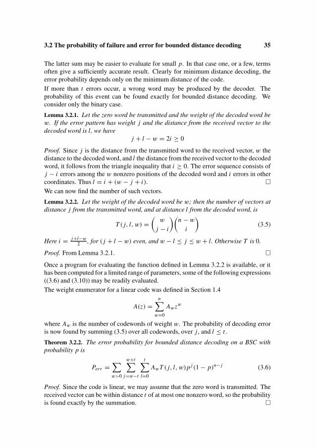
Lemma 3.2.1. Let the zero word be transmitted and the weight of the decoded word bew. If the error pattern has weight j and the distance from the received vector to thedecoded word is l, we have
j + l − w = 2i ≥ 0
Proof. Since j is the distance from the transmitted word to the received vector, w thedistance to the decoded word, and l the distance from the received vector to the decodedword, it follows from the triangle inequality that i ≥ 0. The error sequence consists ofj − i errors among the w nonzero positions of the decoded word and i errors in othercoordinates. Thus l = i + (w − j + i). �We can now find the number of such vectors.
Lemma 3.2.2. Let the weight of the decoded word be w; then the number of vectors atdistance j from the transmitted word, and at distance l from the decoded word, is
T ( j, l, w) =(
w
j − i
)(n − w
i
)(3.5)
Here i = j+l−w2 , for ( j + l − w) even, and w − l ≤ j ≤ w + l. Otherwise T is 0.
Proof. From Lemma 3.2.1. �Once a program for evaluating the function defined in Lemma 3.2.2 is available, or ithas been computed for a limited range of parameters, some of the following expressions((3.6) and (3.10)) may be readily evaluated.
The weight enumerator for a linear code was defined in Section 1.4
A(z) =n∑
w=0
Awzw
where Aw is the number of codewords of weight w. The probability of decoding erroris now found by summing (3.5) over all codewords, over j , and l ≤ t .
Theorem 3.2.2. The error probability for bounded distance decoding on a BSC withprobability p is
Perr =∑w>0
w+t∑j=w−t
t∑l=0
AwT ( j, l, w)p j (1 − p)n− j (3.6)
Proof. Since the code is linear, we may assume that the zero word is transmitted. Thereceived vector can be within distance t of at most one nonzero word, so the probabilityis found exactly by the summation. �

36 Bounds on error probability for error-correcting codes
11
01
00
10
11
01
00
1011
01
00
10
yx
z
w
j
i, l
Figure 3.1: A (6, 3, 3) code is obtained from the codewords listed in Ex-ample 1.1.2 by eliminating the first symbol in the eight codewords thatstart with a ‘0’. In the figure, x represents the first two bits of a code-word, y the next two, and z the last. Vectors with Hamming distance 1are represented as neighbors in this way, and it is readily checked that theHamming distance between codewords is at least 3. The lines illustrateLemma 3.2.2: There is a vector at distance 4 from the zero word and atdistance s = 1 from a codeword of weight w = 3. In this case i = 1.
Theorem 3.2.2 indicates that the weight enumerator contains the information requiredto find the error probability. However, finding the weight enumerator usually requiresextensive computations. It is usually possible to get a sufficiently good approximationby expanding (3.6) in powers of p and only include a few terms.
Example 3.2.1. Error probability of the (16, 11, 4) extended Hamming code.
The code can correct one error. Two errors are detected, but not corrected. Thus we may find theprobability of decoding failure from (3.4) as
Pfail = 1 − (1 − p)16 − 16p(1 − p)15 = 120p2 + · · ·
If p is not very large, decoding errors occur mostly as a result of three errors. From (3.5) wefind T (3, 1, 4) = 4, and Perr can be found from (3.6) using A4 = 140. Actually three errors arealways decoded to a wrong codeword. Thus the first term of the expansion in powers of p is
Perr = 560p3 + · · ·

3.3 Bounds for maximum likelihood decoding of binary block codes 37
3.3 Bounds for maximum likelihood decoding of binaryblock codes
It is often possible to decode more than d2 errors, but for such algorithms it is much
more difficult to calculate the exact error probability. In this section we give somebounds for this case.
The following concept is particularly important:
Definition 3.3.1. Maximum likelihood (ML) decoding maps any received vector, r , to acodeword c such that the distance d(r, c) is minimized.
The term likelihood refers to the conditional probability of receiving r given that c istransmitted. If we assume that all codewords are used equally often, ML decodingminimizes the probability of decoding error. If the closest codeword is not unique, wechoose one of them. The corresponding error patterns are then corrected while othererror patterns of the same weight cause decoding error. In Section 1.3 we discussedhow decoding could be based on syndrome tables. In principle one error pattern ineach coset may be decoded, and if these error patterns are known, we could extendthe summation in (3.4) and calculate the error probability. However, this approach isfeasible only for short codes.
This section gives some upper bounds for the error probability of ML decoding ofbinary codes. These bounds depend only on the weight enumerator, and as for Theo-rem 3.2.1 it is often sufficient to know the first terms of the numerator.
Theorem 3.3.1. For a code with weight enumerator A(z) used on the BSC with bit errorprobability p, an upper bound on the probability of decoding error is
Perr ≤∑w>0
∑j> w
2
Aw
(w
j
)p j (1 − p)w− j + 1
2
∑j>0
A2 j
(2 j
j
)p j (1 − p) j (3.7)
Proof. Since the code is linear, we may assume that the zero word is transmitted. Anerror occurs if the received vector is closer to some nonzero codeword than to the zerovector. For each codeword of odd weight w > 0, the probability that the receivedcodeword is closer to this codeword than to the zero word is
∑j> w
2
(w
j
)p j (1 − p)w− j
since there must be errors in more than w2 of the positions where the nonzero codeword
has a 1. We now get an upper bound on the probability of the union of these events bytaking the sum of their probabilities. When w is even and there are errors in half ofthe positions, there are at least two codewords at distance w
2 . If a pattern of weight w2
occurs only in a single nonzero codeword, a decoding error is made with probability 12 .
If the same pattern occurs in more than one word, the error probability is higher, butthe pattern is then counted with weight 1
2 at least twice in (3.7). �

38 Bounds on error probability for error-correcting codes
Because most errors occur for j close to w2 , we can use this value of j for all error
patterns. Since half of all error patterns have weights greater than w2 , we now find a
simpler approximation
Perr <∑w>0
Aw2w−1(p − p2)w2 (3.8)
Introducing the function Z =√4 p(1− p), which depends only on the channel, we get
Perr <1
2
∑w>0
Aw Zw (3.9)
This is a useful bound when the number of errors corrected is fairly large. Equations(3.7) and (3.9) indicate that the error probability depends not only on the minimumdistance, but also on the number of low weight codewords. As p increases, codewordsof higher weight may contribute more to the error probability, because their number ismuch greater.
In (3.7) we overestimate the error probability whenever a vector is closer to more thanone nonzero word than to the zero word. Actually even an error pattern of weight d
2may be equally close to the zero word and to several nonzero words, but that usuallyhappens only in relatively few cases.
When calculating the terms in (3.7) we do not specify the value of the error patternsoutside the w positions under consideration. Thus if there are several errors in other po-sitions, it is more likely that the vector is also close to another codeword, and vectors ofhigh weight are clearly counted many times (but of course they have small probability).We can get a better bound by keeping track of the weight of the entire error pattern.
The number of error patterns of weight j > w2 that are closer to a particular nonzero
word of weight w than to the zero word may be found using Lemma 3.2.2 as:∑j≥ w
2
∑l< j
T ( j, l, w)
We may again take a union bound by multiplying this number by Aw and summing overw. This sum is an upper bound on the number of errors of weight j that may cause adecoding error. As long as the j -th term is less than the total number of weight j vec-tors, we include it in the bound. However, when j becomes larger, we simply assumethat all vectors of weight j cause errors. Thus the bound (Poltyrev’s bound) becomes
Theorem 3.3.2. For an (n, k, d) code used on the BSC with transition probability p, anupper bound on the error probability is
Perr ≤∑w>0
Aw
∑w2 < j≤J
∑l< j
T ( j, l, w)p j (1 − p)n− j (3.10)
+∑j>J
(n
j
)p j (1 − p)n− j + 1
2
∑l>0
∑l≤ j≤J
A2l T ( j, j, 2l)p j(1 − p)n− j

3.4 Problems 39
Equation (3.10) is true for any choice of J , but the value should be chosen to minimizethe left side. As in (3.7) an extra term has been added to account for error patterns ofweight w
2 . This bound usually gives an excellent approximation to the actual probabil-ity of error with maximum likelihood decoding for all p of interest.
Example 3.3.1. Consider the (16, 5, 8) code with weight distribution A(z) = 1 + 30z8 + z16.Using (3.7) we get the bound
Perr ≤ 30
[1
2
(8
4
)p4(1 − p)4 +
(8
5
)p5(1 − p)3 + · · ·
]
In Theorem 3.3.2 we may include the weight 4 errors in the same way, and we again get30 · 35 = 1050 as the first term. Among error patterns of weight 5 we find the 30 · 56 included inthe expression above, which are patterns with five errors among the eight positions of a nonzeroword. However, there are additional error patterns obtained by adding a single error to a weight4 error pattern in any of the eight zero coordinates of the codeword. These errors were implicit inthe first term, but by counting them explicitly we see that the number, 1050 · 8+30 · 56 = 10080exceeds the total number of weight 5 vectors, 4368. Thus the bound should be
Perr ≤ 1050p4(1 − p)12 +(
16
5
)p5(1 − p)11 +
(16
6
)p6(1 − p)10
A more detailed analysis shows that some 4-tuples are shared between the codewords, and thusthe number of weight 4 errors is slightly overestimated. Actually some weight 5 errors are alsocorrected, and thus the second term is also a little too large.
3.4 ProblemsProblem 3.4.1 Consider the (16, 11, 4) code used on a BSC with p = 0.01.
1) What is the mean value and the standard deviation of the number of errors in a block?
2) What are the probabilities of 0, 1, 2, 3, and 4 errors?
3) Compare these results to the approximation using the Poisson distribution.
4) What is the probability of decoding failure?
5) What is the probability of decoding error (as indicated in Example 3.2.1 this number is closelyapproximated by the probability of 3 errors)?
Problem 3.4.2 The weight distribution of a (15, 7) code is
[1, 0, 0, 0, 0, 18, 30, 15, 15, 30, 18, 0, 0, 0, 0, 1]1) How many errors can the code correct?
Assume minimum distance decoding.
2) If the error probability is p = 0.01, what is the probability of decoding failure?
3) How many error patterns of weight 3 cause decoding error (either an exact number or a goodupper bound)?
4) Give an approximate value of the probability of decoding error based on (3.6).
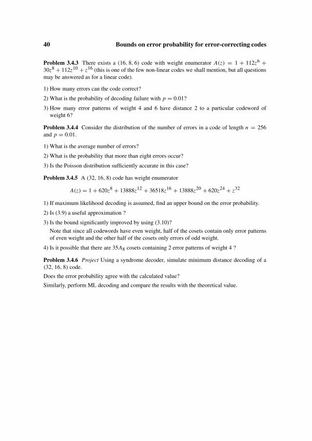
40 Bounds on error probability for error-correcting codes
Problem 3.4.3 There exists a (16, 8, 6) code with weight enumerator A(z) = 1 + 112z6 +30z8 + 112z10 + z16 (this is one of the few non-linear codes we shall mention, but all questionsmay be answered as for a linear code).
1) How many errors can the code correct?
2) What is the probability of decoding failure with p = 0.01?
3) How many error patterns of weight 4 and 6 have distance 2 to a particular codeword ofweight 6?
Problem 3.4.4 Consider the distribution of the number of errors in a code of length n = 256and p = 0.01.
1) What is the average number of errors?
2) What is the probability that more than eight errors occur?
3) Is the Poisson distribution sufficiently accurate in this case?
Problem 3.4.5 A (32, 16, 8) code has weight enumerator
A(z) = 1 + 620z8 + 13888z12 + 36518z16 + 13888z20 + 620z24 + z32
1) If maximum likelihood decoding is assumed, find an upper bound on the error probability.
2) Is (3.9) a useful approximation ?
3) Is the bound significantly improved by using (3.10)?
Note that since all codewords have even weight, half of the cosets contain only error patternsof even weight and the other half of the cosets only errors of odd weight.
4) Is it possible that there are 35A8 cosets containing 2 error patterns of weight 4 ?
Problem 3.4.6 Project Using a syndrome decoder, simulate minimum distance decoding of a(32, 16, 8) code.
Does the error probability agree with the calculated value?
Similarly, perform ML decoding and compare the results with the theoretical value.

Chapter 4
Communication channels andinformation theory
In Chapter 3 we discussed the Binary Symmetric Channel as a model of independenterrors in a transmitted sequence. We now give a more general treatment of modelsof communication channels. An information channel is a model of a communicationlink or a related system where the input is a message and the output is an imperfectreproduction of it. The discussion is based on results from information theory, whichprovides ways of measuring the amounts of information that can be transferred throughchannels with given properties.
4.1 Discrete messages and entropyTo discuss how information is transmitted through a channel that introduces errors weneed at least a simple model of the messages we want to transmit. We assume that thesender has an unlimited amount of data that he, or she, wants to send to a receiver. Thedata is divided into messages, which we usually assume to be strings of independentbinary symbols. One reason for using this particular kind of message is that it is oftenpossible to convert a more realistic message into a string of binary data. We shall give amore formal model of the messages here, because the concepts involved will be neededfor describing the channels.
For a discrete memoryless source the output is a sequence of independent randomvariables with the same properties. Each output, X , has values in a finite alphabet{x1, x2, . . . , xr }. The probability of x j is P(x j ) = p j . It is often convenient to refer tothe probability distribution of X as the vector Q(X) = (p1, p2, . . . , pr ). As a measureof the amount of information represented by X we define
Definition 4.1.1. The entropy of a discrete memoryless source, X, is
H (X) = E[− log P(X)
] = −∑
j
p j log p j (4.1)

42 Communication channels and information theory
where E indicates the expected value. Usually the logarithms are taken with base 2 inthis context, and the (dimensionless) unit of information is a bit.
We note that for an alphabet of r symbols, the maximal value of H is log r , and thisvalue is reached when all symbols have probability 1
r .
Example 4.1.1. The entropy of a discrete source
A source has an alphabet of four symbols with probability distribution(
12 , 1
4 , 18 , 1
8
). If the
symbols all had probability 14 , the entropy would be two bits. Now we find
H = 1
2log 2 + 1
4log 4 + 1
8log 8 + 1
8log 8 = 1
2+ 1
2+ 3
4= 7
4
The source symbols may be represented by on the average 74 binary symbols if we use the source
code a : 0, b : 10, c : 110, d : 111.
The importance of the information theoretic quantities is related to the coding theo-rems, which indicate that sequences of symbols can be mapped into a standard repre-sentation with the same information content, usually binary symbols. Thus an encodermaps (a fixed or variable) number of source symbols to a (fixed or variable) numberof binary encoded symbols such that (on the average) N source symbols are mappedto approximately N H (X) encoded symbols. The code in Example 4.1.1 is a simpleexample of a variable length source code. Most interesting sources are more compli-cated, and in particular they have memory. Coding for such sources is often referred toas data compression.
4.2 Mutual information andcapacity of discrete channels
An information channel is a model of a communication link or a related system wherethe input is a message and the output is an imperfect reproduction of it. The chan-nel may describe a number of restrictions on the message and various transmissionimpairments.
In this section we introduce the concept of mutual information as a measure of theamount of information that flows through the channel, and we shall define the capacityof a channel.
4.2.1 Discrete memoryless channels
In a discrete memoryless channel the input and output are sequences of symbols, andthe current output depends only on the current input. The channel connects a pairof random variables, (X, Y ), with values from finite alphabets {x1, x2, . . . , xr } and{y1, y2, . . . , ys}. The channel is described by the conditional probability of yi given x j ,P(yi |x j ) = p j i . It is often convenient to represent the channel by the transition matrixQ(Y |X) = [p j i ]. The probability distribution of the output variable, Y , then becomes
Q(Y ) = Q(X)Q(Y |X)

4.2 Mutual information and capacity of discrete channels 43
As a measure of the amount of information about X represented by Y we define
Definition 4.2.1. The mutual information of the pair, (X, Y ) is
I (X; Y ) = E
[log
P(y|x)
P(y)
]=∑
j
P(x j )∑
i
p j i[log p j i − log P(yi )
](4.2)
We note that for a given X , the mutual information I (X; Y ) cannot exceed H (X). Thisvalue is reached when Q is a unit matrix, i.e. each value of X corresponds to a uniquevalue of Y , since in that case P(X, Y ) = P(Y ).
It may also be noted that I (Y ; X) = I (X; Y ). The symmetry follows from rewritingP(Y |X) as P(Y,X)
P(X)in the definition of I . This is an unexpected property since we tend
to think of the flow of information going from X to Y (carried by a flow of energy).But actually we may interpret I as the amount of information about Y provided byX .
Lemma 4.2.1. I (X; Y ) = H (Y ) − H (Y |X) = H (X) − H (X |Y ).
This follows immediately from the definition and is a convenient way of calculating I .Usually it is easier to calculate I from the first form, and this calculation is indicated onthe right side of (4.2). The term H (Y |X) can be found from the transition probabilitiesof the channel, and H (Y ) is found from the output distribution, which is obtained bymultiplying the input distribution by the transition matrix. To use the second form weneed to calculate H (X |Y ) from the reverse transition probabilities.
Definition 4.2.2. The capacity of a discrete channel, C(Y |X) is the maximum of I withrespect to P(X).
The definition of capacity may appear straightforward, but analytical solutions are of-ten difficult. In many cases of interest, the symmetry of the transition probabilitiessuggests that the maximum is obtained with symmetric input probabilities. If neces-sary the maximum over a few parameters can be computed numerically.
Example 4.2.1. The binary symmetric channel
The single most important channel model is the binary symmetric channel, (BSC). This channelmodels a situation where random errors occur with probability p in binary data. The transitionmatrix is
Q =(
1 − p pp 1 − p
)
For equally distributed inputs, the output has the same distribution, and the mutual informationmay be found from Lemma 4.2.1 as (in bits/symbol)
C = 1 − H(p) (4.3)
where H is the binary entropy function
H(p) = −p log p − (1 − p) log(1 − p) (4.4)

44 Communication channels and information theory
The entropy function is symmetrical with respect to p = 12 , and reaches its maximal value, 1,
there. Thus the capacity of the BSC drops to 0, which is expected since the output is independentof the input. For small p the capacity decreases quickly with increasing p, and for p = 0.11, weget C = 1
2 .
For a long (n, k) block code, we expect the number of errors to be close to np. For thecode to correct this number of errors it is necessary that the number of syndromes, 2n−k
is at least equal to the number of error patterns (this is the Hamming bound). We relatethis result to the capacity of the channel through the following useful approximation tothe binomial coefficients:
Lemma 4.2.2.m∑
j=0
(n
j
)≤ 2nH( m
n ) (4.5)
Proof. For mn < 1
2 we can use the binomial expansion to get
1 =(m
n+(
1 − m
n
))n ≥m∑
j=0
(n
j
)(m
n
) j (1 − m
n
)n− j
=m∑
j=0
(n
j
)( mn
1 − mn
) j
(1 − m
n)n ≥
m∑j=0
(n
j
)( mn
1 − mn
)m (1 − m
n
)n
= 2−nH( mn )
m∑j=0
(n
j
)
and the inequality follows. �Thus np errors can be corrected only if H (p) < 1 − k
n , i.e. R = kn < C .
The main difficulty in proving that one can get a small probability of decoding errorfor rates close to capacity is related to the fact that it is not possible to construct longcodes that reach the Hamming bound. Thus while it is possible to correct most errorsof weight close to np, not all errors can be corrected.
Example 4.2.2. The binary erasure channel
We say that the channel erases symbols if it outputs a special character ? in stead of the one sent.If actual errors do not occur, the transition matrix becomes
Q =(
1 − p p 00 p 1 − p
)
The capacity of this channel, the binary erasure channel, BEC, is easily found from the last ver-sion of Lemma 4.2.1 as C = 1 − p. Thus the information is simply reduced by the fraction ofthe transmitted symbols that are erased. If a long (n, k) code is used on the BEC, the syndromeequations provide a system of linear equations that may be solved to give the erased symbols.If close to np symbols are erased and the rate of the code is less than 1 − p, there are more

4.2 Mutual information and capacity of discrete channels 45
equations than variables. Since we know that at least the transmitted word is a solution, it isusually unique. However, for any set of j columns of the matrix to be linearly independent, wemust have j < d , and for a binary code d is much smaller than n − k. Thus it is not alwayspossible to correct the erasures.
Example 4.2.3. Let the transition matrix of a discrete channel be
Q =
12
12 0 0
0 12
12 0
0 0 12
12
12 0 0 1
2
Because of the symmetry, all the input symbols may be chosen to have probability 14 . The mu-
tual information is then readily calculated from Lemma 4.2.1 as I = 1. This value cannot beincreased by changing the input distribution, but it is more convenient to use symbols 1 and 3with probability 1
2 , and in this case one bit is transmitted without error.
Other discrete channels may be used as models of the signal processing in modula-tors/demodulators (modems). Many channel models of practical interest are derivedby assuming that the input symbols are real values, and that the channel adds indepen-dent Gaussian noise of zero mean and some variance to the input. In Appendix A wediscuss coding for such channels and give the capacity of a Gaussian noise channel.
4.2.2 Codes and channel capacity
The importance of the capacity is related to coding theorems, which indicate that kmessage bits can be reliably communicated by using the channel a little more thann = k
C times. Thus an encoder maps the k message bits to n encoded symbols usinga code consisting of 2k vectors. A coding theorem states that for any code length, n,and for any rate R < C (in bits per channel symbol), there is a positive constant, E(R)
such that for some codes the error probability satisfies
P(e) < 2−N E(R) (4.6)
For most channels of interest it has not been possible to give direct proofs by construct-ing good codes. Instead the proofs rely on averages over large sets of codes. We givean outline of a proof for the BSC.
If a class of linear block codes use all nonzero vectors with equal probability, the av-erage weight enumerator is obtained by scaling the binomial distribution to the rightnumber of words.
A(z) = 1 +∑w>0
2−n+k(
n
w
)zw (4.7)
It may be noted that with this distribution Theorem 1.4.1 gives a B(z) of the same formwith k ′ = n − k. For small weight, w, the number of codewords is less than 1, and
46 Communication channels and information theory
the Varshamov-Gilbert bound, Theorem 1.2.2 indicates the first weight where the dis-tribution exceeds 1. Combining the bound (3.9) with this weight distribution we getthe following result:
Theorem 4.2.1. For rates R < R0 and any block length n there exist block codes suchthat the error probability on a BSC satisfies
P(e) < 2−n(R0−R) (4.8)
whereR0 = 1 − log(1 + Z) (4.9)
Proof. From (3.9) and (4.5) we get
P(e) < 2−n+k+nH( wn )+w log(Z)
The channel parameter Z = √4 p(1 − p) was introduced in Chapter 3. Here we find
the exponent in the bound by taking the largest term, which occurs for wN = Z
1+Z . Theresult then follows. �A different method is needed to obtain a positive exponent for rates close to capacity.
For a memoryless channel, we can reach the maximal value of I by using independentinputs. However, it is not clear how such symbols could be used for communicating amessage efficiently. If we want to transmit k information bits reliably, we must use thechannel at least n = k
C times in order to get enough information. A block code is ex-actly a rule for selecting a vector of n symbols in such a way that with high probabilitywe can recover the message from the received vector.
When the inputs are no longer independent, less information is in general transmit-ted through the channel. In principle the loss could be calculated by converting thechannel into a vector channel. Now the input is one of the 2k equally likely messagevectors, and since the channel is memoryless, the transition probabilities are found asthe product of the symbol probabilities.
We can now derive some information from Lemma 4.2.1: Assume that we want toget the mutual information close to k = nC . One version of the lemma gives thatH (X) = k, so H (X |Y ) should be zero. Thus an output vector should almost alwaysindicate a unique transmitted message. The other version of the Lemma gives
H (Y1, Y2, . . . , Yn) ≈ nC + nH (Y |X) = nH (Y )
Thus the output distribution should be close to that of n independent symbols, andthe channel should spread out the output vectors enough to eliminate the effect of theselected input vectors.

4.3 Problems 47
4.3 Problems
Problem 4.3.1 A memoryless source has three symbols and probability distribution(
12 , 1
4 , 14
).
1) What is the entropy of the source?
2) What is the largest entropy of a source with three symbols?
3) Give a variable length binary code for the source.
4) Let ui be a sequence of independent variables with probability distribution(
12 , 1
2
), and let
vi be generated as vi = ui−ui−12 . Find the probability distribution of vi . Is V a memoryless
source? Argue that the entropy of V is 1 bit.
Problem 4.3.2 A memoryless channel has transition probabilities
Q =(
12
38
18 0
0 18
38
12
)
1) Find the output distribution when the input distribution is(
12 , 1
2
).
2) Find the mutual information between input and output for this distribution.
3) What is the channel capacity?
Problem 4.3.3 A binary symmetric channel has transition probability p = 0.05.
1) What is the capacity of the channel?
2) If a code of length 256 is used, what is the average number of errors?
3) What is the Hamming bound on the number of errors that can be corrected with a (256, 160)
code?
4) What would be the probability of decoding error if such a code could be used?
5) What is the Gilbert bound for the same parameters?
Problem 4.3.4 The binary Z channel. In some binary channels one of the input symbols is muchmore likely to be in error than the other. Consider the channel with transition matrix
Q =(
1 01 − p p
)
1) Let the input symbols have probability 12 each. What is the mutual information?
2) How much bigger is the channel capacity for p = 0.1, p = 14 , p = 1
2 ?
3) Find an analytic expression.
Problem 4.3.5 A discrete memoryless channel has 17 input and output symbols, both indicatedby [x1, x2, x3, . . . , x17]. The probability of error, i.e. the probability that Y �= X , is p.
1) What is the channel capacity if all other symbols occur with the same probability, p16 ?
2) What is the capacity if the only error symbols are x( j±1 mod 17) when x j is transmitted andtheir probability is p
2 ?
3) Evaluate the capacities for p = 0.11.


Chapter 5
Reed-Solomon codes andtheir decoding
Reed-Solomon codes were discovered in 1959 and have since then been one of themost important classes of error-correcting codes. The applications range from CDs andDVDs to satellite communications. In this chapter we will describe the Reed-Solomoncodes and also give some decoding algorithms of these codes.
5.1 Basic definitions
Before introducing the codes we will first prove an upper bound on the minimum dis-tance of any code.
Theorem 5.1.1. (The Singleton bound) Let C be an (n, k) code with minimum distanced. Then
d ≤ n − k + 1
Proof. We give three different proofs of the theorem, in one of which we do not assumethat the code is linear.
1) Choose the information vector to consist of k − 1 zeroes and one nonzero. Then theweight of the corresponding codeword is at most (n − k) + 1.
2) The rank of a parity check matrix H for the code is n − k so n − k + 1 columns of Hare linearly dependent. Therefore the minimum number of dependent columns (i.e.d) must be smaller than or equal to n − k + 1.
3) If we delete d − 1 fixed positions from all the qk codewords, they are still differ-ent since each pair differ in at least d positions. There are qn−d+1 vectors with theremaining positions and thus k ≤ n − d + 1 and the result follows. �

50 Reed-Solomon codes and their decoding
Definition 5.1.1. (Reed-Solomon codes)Let x1, . . . , xn be different elements of a finite field Fq . For k ≤ n consider the set Pk
of polynomials in Fq [x] of degree less than k. A Reed-Solomon code consists of thecodewords
( f (x1), f (x2), . . . , f (xn)) where f ∈ Pk
It is clear that the length of the code is n ≤ q . The code is linear since if
c1 = ( f1(x1), . . . , f1(xn)) and c2 = ( f2(x1), . . . , f2(xn)),
then
ac1 + bc2 = (g(x1), . . . , g(xn))
where a, b ∈ Fq and g(x) = a f1(x) + b f2(x).
The polynomials in Pk form a vector space over Fq of dimension k since there arek coefficients. We now invoke a fundamental theorem of algebra (Theorem 2.2.1)twice: Two distinct polynomials cannot generate the same codeword since the differ-ence would be a polynomial of degree < k and it cannot have n zeroes, so the dimen-sion of the code is k. A codeword has weight at least n − k + 1 since a polynomial ofdegree < k can have at most k − 1 zeroes. Combining this with Theorem 5.1.1 we get
Theorem 5.1.2. The minimum distance of an (n, k) Reed-Solomon code is n − k + 1.
In many applications one takes xi = αi−1 , i = 1, 2, . . . , q − 1 where α is a primitiveelement of Fq , so in this case we have xn
i = 1 , i = 1, . . . , n, and n = q − 1.
From the definition of the codes it can be seen that one way of encoding these codes isto take k information symbols i0, i1, . . . , ik−1 and encode them as
(i(x1), i(x2), . . . , i(xn))
where i(x) = ik−1xk−1 + · · · + i1x + i0.
This is a non-systematic encoding; we will describe a systematic encoding in a problemin the next chapter.
Since for Reed-Solomon Codes we must have n ≤ q there are no interesting binarycodes. Codes over Fq where q is a prime make easier examples and in particular thefield F11 is useful for decimal codes, since there is no field with ten elements. Howeverin most practical cases we have q = 2m .
Example 5.1.1. Reed-Solomon codes over F11
Since 2 is a primitive element of F11 we can take xi = 2i−1 mod 11, i = 1, 2, . . . , 10 withk = 5 and i(x) = i4x4 + · · · + i1x + i0; we get as the corresponding codeword as
(i(1), i(2), i(4), i(8), i(5), i(10), i(9), i(7), i(3), i(6))

5.2 Decoding Reed-Solomon Codes 51
So
(1, 0, 0, 0, 0) is encoded into (1, 1, 1, 1, 1, 1, 1, 1, 1, 1)
(0, 1, 0, 0, 0) is encoded into (1, 2, 4, 8, 5, 10, 9, 7, 3, 6)
(0, 0, 1, 0, 0) is encoded into (1, 4, 5, 9, 3, 1, 4, 5, 9, 3)
(0, 0, 0, 1, 0) is encoded into (1, 8, 9, 6, 4, 10, 3, 2, 5, 7)
(0, 0, 0, 0, 1) is encoded into (1, 5, 3, 4, 9, 1, 5, 3, 4, 9)
and these five codewords can be used as the rows of a generator matrix of the code, which is a(10, 5, 6) code over F11.
5.2 Decoding Reed-Solomon CodesIn this section we describe the first of three minimum distance decoding algorithmsfor Reed-Solomon codes (in Chapter 12 we present an algorithm for correcting moreerrors). We will first present the idea and give a formal algorithm later.
Let r = c + e be a received word, and assume that w(e) ≤ t = ⌊ n−k2
⌋. The idea is to
determine a bivariate polynomial
Q(x, y) = Q0(x) + y Q1(x) ∈ Fq [x, y]\{0}such that
1. Q(xi , ri ) = 0, i = 1, . . . , n.
2. deg(Q0) ≤ n − 1 − t .
3. deg(Q1) ≤ n − 1 − t − (k − 1).
The polynomial Q(x, y) is called an interpolating polynomial for the received word.We first prove:
Theorem 5.2.1. There is at least one nonzero polynomial Q(x, y) which satisfies con-ditions 1 − 3.
Proof. The condition 1 gives n homogeneous linear equations in the coefficients andthere are n − 1 − t + 1 + n − 1 − t − (k − 1) + 1 ≥ n + 1 possible coefficients, soindeed the system has a nonzero solution. �We also have
Theorem 5.2.2. If the transmitted word is generated by g(x) and the number of errorsis less than d
2 , then g(x) = −Q0(x)Q1(x)
.
Proof. c = (g(x1), . . . , g(xn)) and r = c + e with w(e) ≤ t . The polynomial Q(x, y)
satisfies Q(xi , g(xi ) + ei ) = 0 and since ei = 0 for at least n − t is, we see thatthe univariate polynomial Q(x, g(x)) has at least n − t zeroes, namely the xi s whereg(xi) = ri . But Q(x, g(x)) has degree at most n − t − 1, so Q(x, g(x)) = 0 andtherefore Q0(x) + g(x)Q1(x) = 0 and hence g(x) = − Q0(x)
Q1(x). �
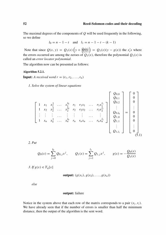
52 Reed-Solomon codes and their decoding
The maximal degrees of the components of Q will be used frequently in the following,so we define
l0 = n − 1 − t and l1 = n − 1 − t − (k − 1)
Note that since Q(x, y) = Q1(x)(
y + Q0(x)Q1(x)
)= Q1(x)(y − g(x)) the x ′
i s where
the errors occurred are among the zeroes of Q1(x), therefore the polynomial Q1(x) iscalled an error locator polynomial.
The algorithm now can be presented as follows:
Algorithm 5.2.1.
Input: A received word r = (r1, r2, . . . , rn)
1. Solve the system of linear equations
1 x1 x21 . . . xl0
1 r1 r1x1 . . . r1xl11
1 x2 x22 . . . xl0
2 r2 r2x2 . . . r2xl12
......
... . . ....
...... . . .
...
1 xn x2n . . . xl0
n rn rn xn . . . rn xl1n
Q0,0Q0,1Q0,2
...
Q0,l0Q1,0Q1,1
...
Q1,l1
=
000...
000...
0
(5.1)
2. Put
Q0(x) =l0∑
j=0
Q0, j x j , Q1(x) =l1∑
j=1
Q1, j x j , g(x) = − Q0(x)
Q1(x)
3. If g(x) ∈ Fq [x]
output: (g(x1), g(x2), . . . , g(xn))
else
output: failure
Notice in the system above that each row of the matrix corresponds to a pair (xi , ri ).We have already seen that if the number of errors is smaller than half the minimumdistance, then the output of the algorithm is the sent word.
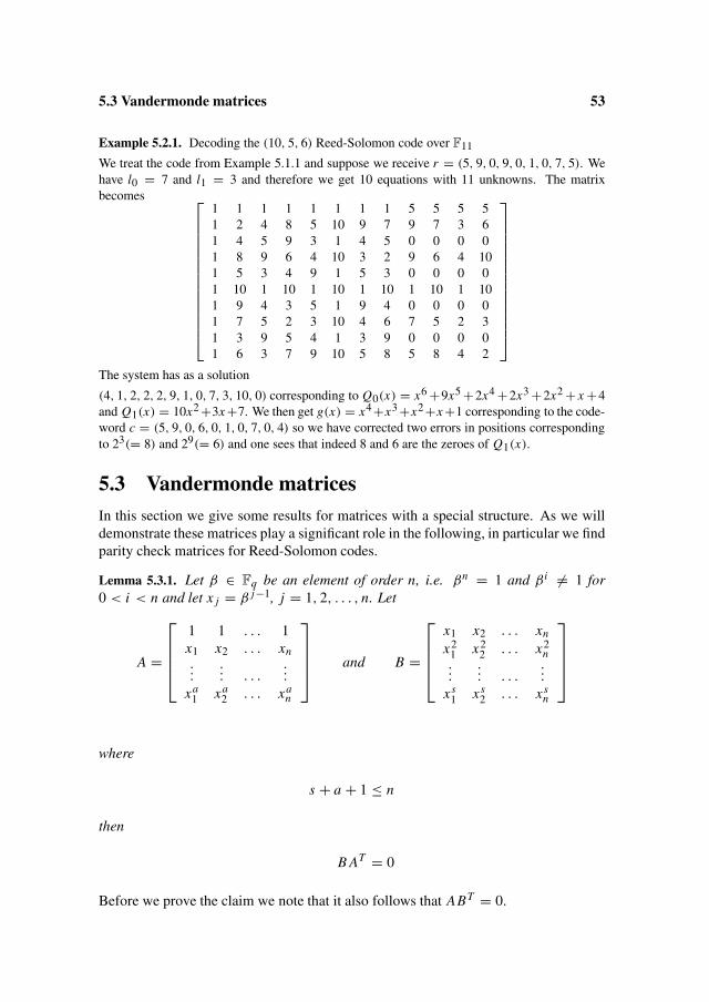
5.3 Vandermonde matrices 53
Example 5.2.1. Decoding the (10, 5, 6) Reed-Solomon code over F11
We treat the code from Example 5.1.1 and suppose we receive r = (5, 9, 0, 9, 0, 1, 0, 7, 5). Wehave l0 = 7 and l1 = 3 and therefore we get 10 equations with 11 unknowns. The matrixbecomes
1 1 1 1 1 1 1 1 5 5 5 51 2 4 8 5 10 9 7 9 7 3 61 4 5 9 3 1 4 5 0 0 0 01 8 9 6 4 10 3 2 9 6 4 101 5 3 4 9 1 5 3 0 0 0 01 10 1 10 1 10 1 10 1 10 1 101 9 4 3 5 1 9 4 0 0 0 01 7 5 2 3 10 4 6 7 5 2 31 3 9 5 4 1 3 9 0 0 0 01 6 3 7 9 10 5 8 5 8 4 2
The system has as a solution
(4, 1, 2, 2, 2, 9, 1, 0, 7, 3, 10, 0) corresponding to Q0(x) = x6 +9x5 +2x4 +2x3 +2x2 + x +4and Q1(x) = 10x2 +3x +7. We then get g(x) = x4 +x3 +x2 +x +1 corresponding to the code-word c = (5, 9, 0, 6, 0, 1, 0, 7, 0, 4) so we have corrected two errors in positions correspondingto 23(= 8) and 29(= 6) and one sees that indeed 8 and 6 are the zeroes of Q1(x).
5.3 Vandermonde matricesIn this section we give some results for matrices with a special structure. As we willdemonstrate these matrices play a significant role in the following, in particular we findparity check matrices for Reed-Solomon codes.
Lemma 5.3.1. Let β ∈ Fq be an element of order n, i.e. βn = 1 and β i �= 1 for0 < i < n and let x j = β j−1, j = 1, 2, . . . , n. Let
A =
1 1 . . . 1x1 x2 . . . xn...
... . . ....
xa1 xa
2 . . . xan
and B =
x1 x2 . . . xn
x21 x2
2 . . . x2n
...... . . .
...
xs1 xs
2 . . . xsn
where
s + a + 1 ≤ n
then
B AT = 0
Before we prove the claim we note that it also follows that ABT = 0.

54 Reed-Solomon codes and their decoding
Proof. Let C = B AT . Since bi j = xij and ar j = xr−1
j we get
cir =n∑
j=1
xij xr−1
j =n∑
j=1
xi+r−1j =
n∑j=1
(β i+r−1
) j−1
Sincei + r − 1 ≤ s + a ≤ n − 1
soβ i+r−1 �= 1
we get
cir =(β i+r−1
)n − 1
β i+r−1 − 1but (
βn)i+r−1 = 1
and the result follows. �If a = n −1 the A-matrix is a so-called Vandermonde matrix, and here the determinantcan be calculated.
Theorem 5.3.1. Let
Dn =
∣∣∣∣∣∣∣∣∣
1 x1 x21 . . . xn−1
11 x2 x2
2 . . . xn−12
......
......
...
1 xn x2n . . . xn−1
n
∣∣∣∣∣∣∣∣∣where xi ∈ Fq .
Then
Dn =n∏
i> j
(xi − x j
)
Proof. By induction on n. We have D2 = x2 − x1. Dn can be considered as a polyno-mial of degree n − 1 in the variable xn . This has zeroes x1, x2, . . . xn−1 and since thecoefficient to xn−1
n is Dn−1 we get
Dn =n−1∏i=1
(xn − xi ) Dn−1
and the result follows. �Corollary 5.3.1.
∣∣∣∣∣∣∣∣∣
xi1 xi2 . . . xitx2
i1x2
i2. . . x2
it...
......
...
xti1
xti2
. . . xtit
∣∣∣∣∣∣∣∣∣= xi1 · · · xit
∏1≤l< j≤t
(xi j − xil
)
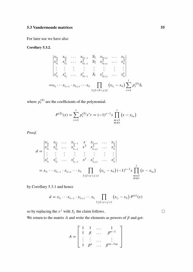
5.3 Vandermonde matrices 55
For later use we have also
Corollary 5.3.2.
∣∣∣∣∣∣∣∣∣
xi1 xi2 . . . xiS−1 S1 xiS+1 . . . xitx2
i1x2
i2. . . x2
iS−1S2 x2
iS+1. . . x2
it...
......
......
......
...
xti1
xti2
. . . xtiS−1
St x tiS+1
. . . xtit
∣∣∣∣∣∣∣∣∣
=xi1 · · · xis−1 · xis+1 · · · xit
∏1≤l<S< j≤t
(xi j − xil
) t∑r=1
p(S)r Sr
where p(S)r are the coefficients of the polynomial.
P(S)(x) =t∑
r=1
p(S)r xrr = (−1)s−1x
t∏m=1m �=s
(x − xim
)
Proof.
d =
∣∣∣∣∣∣∣∣∣
xi1 xi2 . . . xis−1 x xis+1 . . . xitx2
i1x2
i2. . . x2
is−1x2 x2
is+1. . . x2
it...
......
......
......
...
xti1
xti2
. . . xtis−1
xt x tis+1
. . . xtit
∣∣∣∣∣∣∣∣∣
= xi1 · · · xis−1 · xis+1 · · · xit
∏1≤l<s< j<t
(xi j − xil
)(−1)s−1x
t∏m=1m �=s
(x − xim
)
by Corollary 5.3.1 and hence
d = xi1 · · · xis−1 · xis+1 · · · xit
∏1≤l<s< j<t
(xi j − xil
)P(s)(x)
so by replacing the x j with Sj the claim follows. �We return to the matrix A and write the elements as powers of β and get:
A =
1 1 . . . 11 β . . . βn−1
...... . . .
...
1 βa . . . β(n−1)a
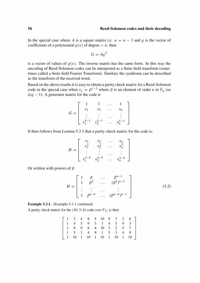
56 Reed-Solomon codes and their decoding
In the special case where A is a square matrix i.e. a = n − 1 and g is the vector ofcoefficients of a polynomial g(x) of degree < n, then
G = AgT
is a vector of values of g(x). The inverse matrix has the same form. In this way theencoding of Reed-Solomon codes can be interpreted as a finite field transform (some-times called a finite field Fourier Transform). Similary the syndrome can be describedas the transform of the received word.
Based on the above results it is easy to obtain a parity check matrix for a Reed-Solomoncode in the special case when x j = β j−1 where β is an element of order n in Fq (son|q − 1). A generator matrix for the code is
G =
1 1 . . . 1x1 x2 . . . xn...
... . . ....
xk−11 xk−1
2 . . . xk−1n
It then follows from Lemma 5.3.1 that a parity check matrix for the code is:
H =
x1 x2 . . . xn
x21 x2
2 . . . x2n
...... . . .
...
xn−k1 xn−k
2 . . . xn−kn
Or written with powers of β
H =
1 β . . . βn−1
1 β2 . . . (β2)n−1
...... . . .
...
1 βn−k . . . (βn−k)n−1
(5.2)
Example 5.3.1. (Example 5.1.1 continued)
A parity check matrix for the (10, 5, 6) code over F11 is then
1 2 4 8 5 10 9 7 3 61 4 5 9 3 1 4 5 9 31 8 9 6 4 10 3 2 5 71 5 3 4 9 1 5 3 4 91 10 1 10 1 10 1 10 1 10

5.4 Another decoding algorithm 57
5.4 Another decoding algorithm
In this section we present another version of minimum distance decoding of RS codes(historically this was the first such algorithm).
We treat the case where xi = β i−1 where β is an element of order n in Fq .
Here the decoding problem is split into two stages. First we find an error locator poly-nomial i.e. Q1(x) and then we determine the error values.
Let r = c + e be a received word with w(e) < d2 . Let the syndrome S = (S1, S2, . . . ,
Sn−k) be
S = Hr T
where H is the parity check matrix( 5.2). With r = (r1, r2, . . . , rn) and r(x) =rn xn−1 + · · · + r2x + r1 this means that
Si = r(β i ) = e(β i).
In the following we also refer to the individual Si s as syndromes.
Theorem 5.4.1. An error locator Q1 is a solution to the system of linear equations
S1 S2 . . . Sl1+1S2 S3 . . . Sl1+2...
... . . ....
Sl1 Sl1+1 . . . S2(l1)
Q1,0Q1,1Q1,2
...
Q1,l1
=
000...
0
Proof. We use the results of Section 5.2 to prove first that if Q1(x) is an error locatorthen the system of equations is satisfied and then if we have a solution to the system ofequations we can get the interpolating polynomial Q(x, y).
We note that the system of equations to determine Q(x, y) can be written as
1 x1 x21 . . . xl0
11 x2 x2
2 . . . xl02
......
... . . ....
1 xn x2n . . . xl0
n
Q0,0Q0,1Q0,2
...
Q0,l0
+
r1 r1x1 . . . r1xl11
r2 r2x2 . . . r2xl12
...... . . .
...
rn rn xn . . . rn xl1n
Q1,0Q1,1Q1,2
...
Q1,l1
=
0...
0
(5.3)

58 Reed-Solomon codes and their decoding
Since the first part of this system is independent of the received word we can remove itby multiplying the system with
B =
x1 x2 . . . xn
x21 x2
2 . . . x2n
...... . . .
...
xl11 xl1
2 . . . xl1n
it follows from Section 5.3 that we get
x1 x2 . . . xn
x21 x2
2 . . . x2n
...... . . .
...
xl11 xl1
2 . . . xl1n
r1 r1x1 . . . r1xl11
r2 r2x2 . . . r2xl12
...... . . .
...
rn rn xn . . . rn xl1n
Q1,0Q1,1Q1,2
...
Q1,l1
=
000...
0
This is the same as
x1 x2 . . . xn
x21 x2
2 . . . x2n
...... . . .
...
xl11 xl1
2 . . . xl1n
r1 . . . 0 00 r2 . . . 0...
.... . . 0
0 0 . . . rn
×
1 x1 . . . xl11
1 x2 . . . xl12
...... . . .
...
1 xn . . . xl1n
Q1,0Q1,1Q1,2
...
Q1,l1
=
000...
0
If we let
D(r) =
x1 x2 . . . xn
x21 x2
2 . . . x2n
...... . . .
...
xl11 xl1
2 . . . xl1n
r1 . . . 0 00 r2 . . . 0...
.... . . 0
0 0 . . . rn
1 x1 . . . xl11
1 x2 . . . xl12
...... . . .
...
1 xn . . . xl1n
then an easy calculation shows that di j = Si+ j−1 , i = 1, . . . , l1 j = 1, . . . , l1 + 1 andthat D(r) = D(e).
So Q1(x) is a solution to the system
S1 S2 . . . Sl1+1S2 S3 . . . Sl1+2...
... . . ....
Sl1 Sl1+1 . . . S2(l1)
Q1,0Q1,1Q1,2
...
Q1,l1
=
000...
0
(5.4)

5.4 Another decoding algorithm 59
On the other hand
If Q1(x) solves (5.4) we have that
x1 x2 . . . xn
x21 x2
2 . . . x2n
...... . . .
...
xl11 xl1
2 . . . xl1n
r1 r1x1 . . . r1xl11
r2 r2x2 . . . r2xl12
...... . . .
...
rn rn xn . . . rn xl1n
Q1,0Q1,1Q1,2
...
Q1,l1
=
000...
0
and therefore the vector
r1 r1x1 . . . r1xl11
r2 r2x2 . . . r2xl12
...... . . .
...
rn rn xn . . . rn xl1n
Q1,0Q1,1Q1,2
...
Q1,l1
is in the nullspace of B .
This, as follows from (5.3), is contained in the space spanned by the columns of
1 x1 x21 . . . xl0
11 x2 x2
2 . . . xl02
......
... . . ....
1 xn x2n . . . xl0
n
and therefore (5.3) has a solution Q0(x). �The above argument holds for any solution Q1(x), so in the case where there is a choicewe select the solution of lowest degree.
When Q1(x) has been determined, its zeroes β i1 , β i2 , . . . β it are found, usually bytesting all q elements of Fq . Since
H eT = (S1, S2, . . . , S2(l1)),
the error values can then be found by solving the system of equations.
xi1 xi2 . . . xitx2
i1x2
i2. . . x2
it...
......
...
xti1
xti2
. . . xtit
ei1ei2...
eit
=
S1S2...
St
(5.5)

60 Reed-Solomon codes and their decoding
By Cramers rule we get
eis =
∣∣∣∣∣∣∣∣∣
xi1 xi2 . . . xiS−1 S1 xiS+1 . . . xitx2
i1x2
i2. . . x2
iS−1S2 x2
iS+1. . . x2
it...
......
......
......
...
xti1
xti2
. . . xtiS−1
St x tiS+1
. . . xtit
∣∣∣∣∣∣∣∣∣∣∣∣∣∣∣∣∣∣
xi1 xi2 . . . xiS−1 xiS xiS+1 . . . xitx2
i1x2
i2. . . x2
iS−1x2
iSx2
iS+1. . . x2
it...
......
......
......
...
xti1
xti2
. . . xtiS−1
xtiS
x tiS+1
. . . xtit
∣∣∣∣∣∣∣∣∣
and therefore using corollaries 5.3.1 and 5.3.2
eiS =xi1 . . . xiS−1 xiS+1 . . . xit
∏1≤l<S< j≤t
(xi j − xil
)
xi1 . . . xit
∏1≤l≤ j≤t
(xi j − xil
)t∑
r=1
P(S)r Sr
=
t∑r=1
P(S)r Sr
P(S)(xiS )(5.6)
We now have the following
Algorithm 5.4.1. Peterson’s
Input: A received word r = (r1, r2, . . . , rn)
1. Calculate the syndromes Si = r(β i), i = 1, 2, . . . , n − k, where r(x) =
rn−1xn−1 + · · · + r1x + r0.
2. Find the solution Q1(x) of lowest degree to the system
S1 S2 . . . Sl1+1S2 S3 . . . Sl1+2...
... . . ....
Sl1 Sl1+1 . . . S2l1
Q1,0Q1,1
...
Q1,l1
=
00...
0
3. Find the zeroes of Q1(x), β i1 , . . . , β it , say.
4. Find the error values by solving the system (5.5) or use the formula (5.6.)
Output: The error vector (e1, e2, . . . , en)
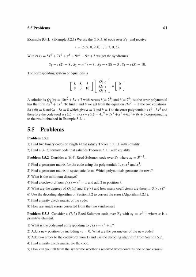
5.5 Problems 61
Example 5.4.1. (Example 5.2.1) We use the (10, 5, 6) code over F11 and receive
r = (5, 9, 0, 9, 0, 1, 0, 7, 0, 5).
With r(x) = 5x9 + 7x7 + x5 + 9x3 + 9x + 5 we get the syndromes
S1 = r(2) = 8 , S2 = r(4) = 8 , S3 = r(8) = 3 , S4 = r(5) = 10.
The corresponding system of equations is
[8 8 38 3 10
]
Q1,0Q1,1Q1,2
=
[00
]
A solution is Q1(x) = 10x2 +3x +7 with zeroes 8(= 23) and 6(= 29), so the error polynomialhas the form bx9 + ax3. To find a and b we get from the equation HeT = S the two equations
8a+6b = 8 and 9a+3b = 8 which give a = 3 and b = 1 so the error polynomial is x9+3x5 andtherefore the codeword is c(x) = w(x)− e(x) = 4x9 + 7x7 + x5 + 6x3 + 9x + 5 correspondingto the result obtained in Example 5.2.1.
5.5 ProblemsProblem 5.5.1
1) Find two binary codes of length 4 that satisfy Theorem 5.1.1 with equality.
2) Find a (4, 2) ternary code that satisfies Theorem 5.1.1 with equality.
Problem 5.5.2 Consider a (6, 4) Reed-Solomon code over F7 where xi = 3i−1.
1) Find a generator matrix for the code using the polynomials 1, x, x2 and x3.
2) Find a generator matrix in systematic form. Which polynomials generate the rows?
3) What is the minimum distance?
4) Find a codeword from f (x) = x3 + x and add 2 to position 3.
5) What are the degrees of Q0(x) and Q1(x) and how many coefficients are there in Q(x, y)?
6) Use the decoding algorithm of Section 5.2 to correct the error (Algorithm 5.2.1).
7) Find a parity check matrix of the code.
8) How are single errors corrected from the two syndromes?
Problem 5.5.3 Consider a (7, 3) Reed-Solomon code over F8 with xi = αi−1 where α is aprimitive element.
1) What is the codeword corresponding to f (x) = x2 + x?
2) Add a new position by including x8 = 0. What are the parameters of the new code?
3) Add two errors to the codeword from 1) and use the decoding algorithm from Section 5.2.
4) Find a parity check matrix for the code.
5) How can you tell from the syndrome whether a received word contains one or two errors?
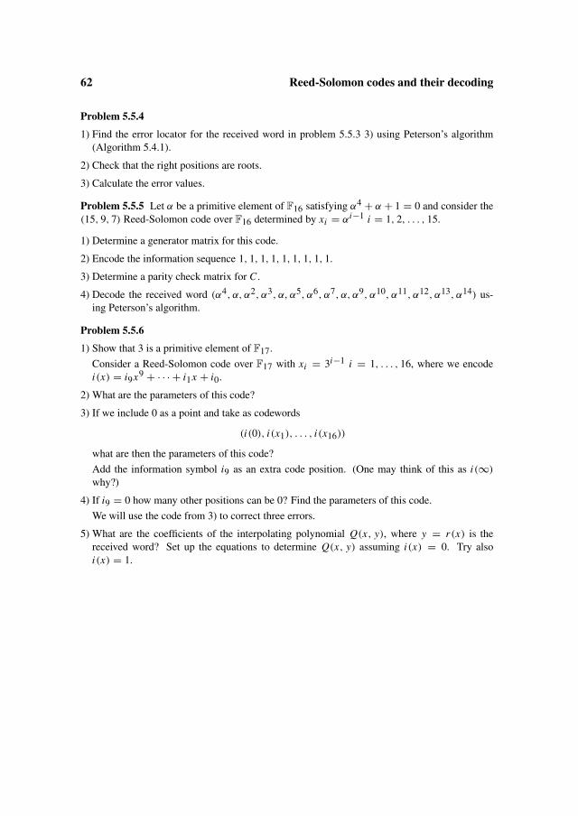
62 Reed-Solomon codes and their decoding
Problem 5.5.4
1) Find the error locator for the received word in problem 5.5.3 3) using Peterson’s algorithm(Algorithm 5.4.1).
2) Check that the right positions are roots.
3) Calculate the error values.
Problem 5.5.5 Let α be a primitive element of F16 satisfying α4 + α + 1 = 0 and consider the(15, 9, 7) Reed-Solomon code over F16 determined by xi = αi−1 i = 1, 2, . . . , 15.
1) Determine a generator matrix for this code.
2) Encode the information sequence 1, 1, 1, 1, 1, 1, 1, 1, 1.
3) Determine a parity check matrix for C .
4) Decode the received word (α4, α, α2, α3, α, α5, α6, α7, α, α9, α10, α11, α12, α13, α14) us-ing Peterson’s algorithm.
Problem 5.5.6
1) Show that 3 is a primitive element of F17.
Consider a Reed-Solomon code over F17 with xi = 3i−1 i = 1, . . . , 16, where we encodei(x) = i9x9 + · · · + i1x + i0.
2) What are the parameters of this code?
3) If we include 0 as a point and take as codewords
(i(0), i(x1), . . . , i(x16))
what are then the parameters of this code?
Add the information symbol i9 as an extra code position. (One may think of this as i(∞)
why?)
4) If i9 = 0 how many other positions can be 0? Find the parameters of this code.
We will use the code from 3) to correct three errors.
5) What are the coefficients of the interpolating polynomial Q(x, y), where y = r(x) is thereceived word? Set up the equations to determine Q(x, y) assuming i(x) = 0. Try alsoi(x) = 1.
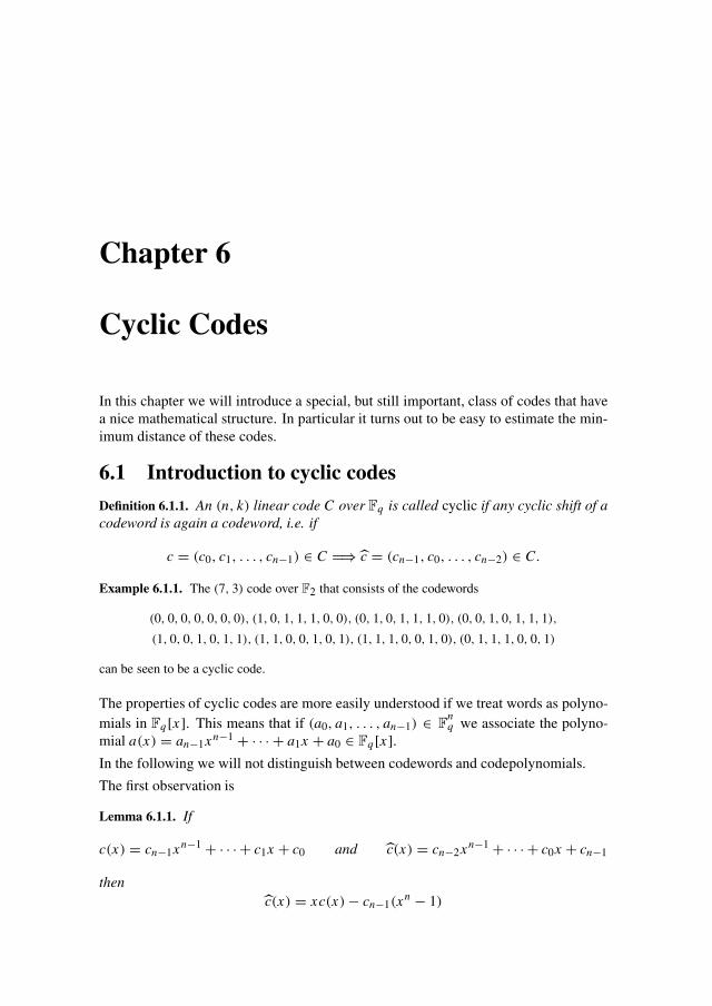
Chapter 6
Cyclic Codes
In this chapter we will introduce a special, but still important, class of codes that havea nice mathematical structure. In particular it turns out to be easy to estimate the min-imum distance of these codes.
6.1 Introduction to cyclic codes
Definition 6.1.1. An (n, k) linear code C over Fq is called cyclic if any cyclic shift of acodeword is again a codeword, i.e. if
c = (c0, c1, . . . , cn−1) ∈ C =⇒ c = (cn−1, c0, . . . , cn−2) ∈ C.
Example 6.1.1. The (7, 3) code over F2 that consists of the codewords
(0, 0, 0, 0, 0, 0, 0), (1, 0, 1, 1, 1, 0, 0), (0, 1, 0, 1, 1, 1, 0), (0, 0, 1, 0, 1, 1, 1),
(1, 0, 0, 1, 0, 1, 1), (1, 1, 0, 0, 1, 0, 1), (1, 1, 1, 0, 0, 1, 0), (0, 1, 1, 1, 0, 0, 1)
can be seen to be a cyclic code.
The properties of cyclic codes are more easily understood if we treat words as polyno-mials in Fq [x]. This means that if (a0, a1, . . . , an−1) ∈ n
Fq we associate the polyno-mial a(x) = an−1xn−1 + · · · + a1x + a0 ∈ Fq [x].In the following we will not distinguish between codewords and codepolynomials.
The first observation is
Lemma 6.1.1. If
c(x) = cn−1xn−1 + · · · + c1x + c0 and c(x) = cn−2xn−1 + · · · + c0x + cn−1
thenc(x) = xc(x) − cn−1(xn − 1)

64 Cyclic Codes
The lemma is proved by direct calculation.
Theorem 6.1.1. Let C be a cyclic (n, k) code over Fq and let g(x) be the monic poly-nomial of lowest degree in C\{0}.Then
1. g(x) divides c(x) for every c ∈ C.
2. g(x) divides xn − 1 in Fq [x].3. k = n − deg(g(x)).
We first note that g(x) is uniquely determined, since if there were two, their difference(since the code is linear) would have lower degree and would be a codeword.
Proof of the theorem.
It is clear from the definition of g(x) that k ≤ n − deg(g(x)), since there are onlyn − deg(g(x)) positions left.
If g(x) has degree s, then g(x) = gs−1xs−1 +· · ·+g1x +g0+xs so from Lemma 6.1.1we get that x j g(x) is in C if j ≤ n − 1 − s. Therefore a(x)g(x) where deg(a(x)) ≤n − 1 − s are also codewords of C .
It is also easy to see that x j g(x) where j ≤ n − 1 − s are linearly independent code-words of C , so k ≥ n − s, and we then have k = n − s, proving 3.
To prove 1, suppose c(x) ∈ C then c(x) = a(x)g(x) + r(x) where deg(r(x)) <
deg(g(x)). Since deg(a(x)) ≤ n − 1 − s we have that a(x)g(x) is a codeword andtherefore that r(x) = c(x)−a(x)g(x) is also in the code. Since deg(r(x)) < deg(g(x))
this implies that r(x) = 0 and therefore g(x) divides c(x), and 1 is proved.
2 follows directly from the lemma since g(x) divides c(x) and also c(x). �The polynomial g(x) in the theorem is called the generator polynomial for the cycliccode C .
Example 6.1.2. (Example 6.1.1 continued) We see that g(x) = x4 + x3 + x2 + 1 and thatthe codewords all have the form (a2x2 + a1x + a0)g(x) where ai ∈ F2 and that x7 − 1 =(x4 + x3 + x2 + 1)(x3 + x2 + 1).
So to a cyclic code corresponds a divisor of xn − 1 and a natural question is thereforeif there to any divisor of xn − 1 corresponds a cyclic code. We answer that in theaffirmative in
Theorem 6.1.2. Suppose g(x) ∈ Fq [x] is monic and divides xn − 1.
Then C = {i(x)g(x)|i(x) ∈ Fq [x], deg(i(x)) < n − deg(g(x))} is a cyclic code withgenerator polynomial g(x).
Proof. It is obvious that C is a linear code, and if it is cyclic the generator polynomial isg(x) and hence the dimension is n−deg(g(x)) so we only have to prove that C is cyclic.

6.2 Generator- and parity check matrices of cyclic codes 65
To this end let g(x) = gs−1xs−1 + · · · + g1x + g0 + xs and h(x) = (xn−1)g(x)
=xn−s + hn−s−1xn−s−1 + · · · + h1x + h0.
Let c(x) = i(x)g(x) where deg(i(x)) < n − s, then
c(x) = xc(x)−cn−1(xn −1) = xi(x)g(x)−cn−1h(x)g(x) = (xi(x)−cn−1h(x))g(x).
Now cn−1 = in−s−1 so indeed (xi(x) − cn−1h(x)) has deg < n − s and therefore c(x)
is also in C . �The two theorems combined tell us that we can study cyclic codes by studying the di-visors of xn − 1. In the case q = 2 and n odd we gave a method for finding divisors ofxn − 1 in Section 2.3.
Example 6.1.3. Binary cyclic codes of length 21
Using the algorithm of Section 2.3 we have
x21−1 = (x−1)(x6+x4+x2+x+1)(x3+x2+1)(x6+x5+x4+x2+1)(x2+x+1)(x3+x+1).
With g(x) = (x6 + x4 + x2 + x + 1)(x3 + x2 + 1) we get a (21, 12) binary code. Withg1(x) = (x6 + x4 + x2 + x + 1)(x3 + x + 1) we also get a (21, 12) code.
6.2 Generator- and parity check matricesof cyclic codes
Let C be an (n, k) cyclic code over Fq . As proved in Section 6.1 the code C has a gen-erator polynomial g(x) of degree n − k, that is g(x) = xn−k + gn−k−1xn−k−1 + · · · +g1x + g0 and we also saw that x j g(x), j = 0, 1, . . . , k − 1 gave linearly independentcodewords. This means that a generatormatrix of C is
G =
g0 g1 g2 . . .
0 g0 g1 . . .
0 0 g0 . . ....
......
. . .
So G has as its first row the coefficients of g(x) and the remaining k − 1 rows areobtained as cyclic shifts.
To get a parity check matrix we observe that g(x)h(x) = xn−1, since h(x) was definedexactly in this way and, if c(x) = i(x)g(x), we get that c(x)h(x) = i(x)g(x)h(x) =i(x)(xn − 1) so the polynomial c(x)h(x) does not contain any terms of degrees k, k +1, . . . , n −1 and therefore
∑n−1i=0 ci h j−i = 0 for j = k, k +1, . . . , n −1, where hs = 0
if s < 0.
From this we get that the vectors
(hk, hk−1, . . . , h0, 0, . . . , 0), . . . , (0, . . . , hk, hk−1, . . . , h0)

66 Cyclic Codes
give n − k independent parity check equations so a parity check matrix is
H =
hk hk−1 hk−2 . . .
0 hk hk−1 . . .
0 0 hk . . ....
......
. . .
So H has as its first row the coefficients of h(x) in reverse order and the remainingn − k − 1 rows are cyclic shifts of the first row. Therefore we have
Theorem 6.2.1. If C is an (n, k) cyclic code with generator polynomial g(x), then thedual code C⊥ is also cyclic and has generator polynomial g⊥(x) = h0xk + · · · +hk−1x + hk = xkh(x−1) where h(x) = xn−1
g(x)
Example 6.2.1. For the code considered in Example 6.1.1 we get
G =
1 0 1 1 1 0 00 1 0 1 1 1 00 0 1 0 1 1 1
and
H =
1 1 0 1 0 0 00 1 1 0 1 0 00 0 1 1 0 1 00 0 0 1 1 0 1
6.3 A theorem on the minimum distance of cyclic codes
In this section we prove a lower bound on the minimum distance of a cyclic code (theso-called BCH-bound).
Theorem 6.3.1. Let g(x) be the generator polynomial of a cyclic (n, k) code C overFq and suppose that g(x) has among its zeroes βa, βa+1, . . . , βa+d−2 where β ∈ m
Fq
has order n.
Then dmin(C) ≥ d.
Proof.
H =
1 βa β2a . . . βa(n−1)
......
... . . ....
......
... . . ....
1 βa+d−2 β2(a+d−2) . . . β(n−1)(a+d−2)

6.4 Cyclic Reed-Solomon codes and BCH-codes 67
is a parity check matrix of C (properly interpreted) and if we take the determinant ofthe matrix consisting of d − 1 coloumns of H we get:
∣∣∣∣∣∣∣∣∣∣
βai1 βai2 . . . βa(id−1)
...... . . .
......
... . . ....
β(a+d−2)i1 β(a+d−2)i2 . . . β(a+d−2)(id−1)
∣∣∣∣∣∣∣∣∣∣
=
∣∣∣∣∣∣∣
xa1 . . . xa
d−1... . . .
...
xa+d−21 . . . xa+d−2
d−1
∣∣∣∣∣∣∣
where x j = β i j . This is then
xa1 . . . xa
d−1
∣∣∣∣∣∣∣∣∣
1 . . . 1x1 . . . xd−1... . . .
...
xd−21 . . . xd−2
d−1
∣∣∣∣∣∣∣∣∣
so from Theorem 5.3.1 we get
xa1 . . . xa
d−1
d−1∏i> j
(xi − x j ) �= 0
So any d − 1 columns are linearly independent and the result follows. �
Example 6.3.1. (Example 6.1.3 continued)
The (21, 12) code with g(x) = (x6 + x4 + x2 + x + 1)(x3 + x2 + 1) = mβ(x)mβ3 (x) = x9 +x8 + x7 + x5 + x4 + x +1 has minimum distance at least 5, since the generator has β, β2, β3, β4
among its zeroes. Since c(x) = (x2 + x + 1)g(x) = x11 + x9 + x4 + x3 + 1 is a codewordthe minimum distance is 5. This is actually best possible. For the (21, 12) code with generatorg1(x) = mβ(x)mβ9 (x) the bound only gives dmin ≥ 3, but the true minimum distance is again 5.
6.4 Cyclic Reed-Solomon codes and BCH-codes
In this section we shall see that a large class of the Reed-Solomon codes as defined inChapter 5 are cyclic codes and we will determine their generator polynomials. We willalso consider (in the case where q = 2m ), the subcode consisting of the binary wordsof the original code and show that this is also a cyclic code with a generator polyno-mial that is easy to determine. It then follows from the definition that indeed we havea lower bound on the minimum distance. We shall also indicate how the Peterson’sdecoding algorithm works for decoding these binary codes.
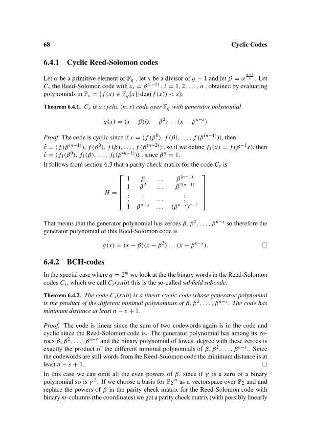
68 Cyclic Codes
6.4.1 Cyclic Reed-Solomon codes
Let α be a primitive element of Fq , let n be a divisor of q − 1 and let β = αq−1
n . LetCs the Reed-Solomon code with xi = β(i−1) , i = 1, 2, . . . , n , obtained by evaluatingpolynomials in Ps = { f (x) ∈ Fq [x]| deg( f (x)) < s}.Theorem 6.4.1. Cs is a cyclic (n, s) code over Fq with generator polynomial
g(x) = (x − β)(x − β2) · · · (x − βn−s)
Proof. The code is cyclic since if c = ( f (β0), f (β), . . . , f (β(n−1))), then
c = ( f (β(n−1)), f (β0), f (β), . . . , f (β(n−2)) , so if we define f1(x) = f (β−1x), thenc = ( f1(β
0), f1(β), . . . , f1(β(n−1))) , since βn = 1.
It follows from section 6.3 that a parity check matrix for the code Cs is
H =
1 β . . . β(n−1)
1 β2 . . . β2(n−1)
...... . . .
...
1 βn−s . . . (βn−s)n−1
That means that the generator polynomial has zeroes β, β2, . . . , βn−s so therefore thegenerator polynomial of this Reed-Solomon code is
g(x) = (x − β)(x − β2) . . . (x − βn−s). �
6.4.2 BCH-codes
In the special case where q = 2m we look at the the binary words in the Reed-Solomoncodes Cs , which we call Cs(sub) this is the so-called subfield subcode.
Theorem 6.4.2. The code Cs(sub) is a linear cyclic code whose generator polynomialis the product of the different minimal polynomials of β, β2, . . . , βn−s . The code hasminimum distance at least n − s + 1.
Proof. The code is linear since the sum of two codewords again is in the code andcyclic since the Reed-Solomon code is. The generator polynomial has among its ze-roes β, β2, . . . , βn−s and the binary polynomial of lowest degree with these zeroes isexactly the product of the different minimal polynomials of β, β2, . . . , βn−s . Sincethe codewords are still words from the Reed-Solomon code the minimum distance is atleast n − s + 1. �In this case we can omit all the even powers of β, since if γ is a zero of a binarypolynomial so is γ 2. If we choose a basis for F2
m as a vectorspace over F2 and andreplace the powers of β in the parity check matrix for the Reed-Solomon code withbinary m-columns (the coordinates) we get a parity check matrix (with possibly linearly

6.4 Cyclic Reed-Solomon codes and BCH-codes 69
dependent rows) for the subfield subcode. From this follows that the dimension ofCs(sub) is at least n − m
( n−s2
). Usually this a very weak bound; in specific cases
where we have the generator polynomial g(x) of course there is no problem since thenk = n − deg(g(x)). The true minimum distance of these codes can be hard to find,however in many cases the bound actually gives the truth. With n = 2m −1 and dmin =2t + 1 we get n − k ≤ t log(n). For low rates this is very close to the Hamming bound.
The codes obtained in this way are called (narrow sense) BCH-codes after Bose,Chaudhuri and Hocquenghem who first considered them. One of the nice things isthat you can guarantee (a lower bound on) the minimum distance of the code, and itwas exactly this that originally was the rationale for the construction.
The Peterson decoding algorithm can be used to decode these codes as well, as we aregoing to illustrate.
Example 6.4.1. Decoding of a (15, 5, 7) BCH-code
This code corresponds to the case where n = 15, s = 9 and q = 24, so the generator polynomialhas among its roots β, β2, . . . , β6 and in this case β = α, where α is a primitive element of F16.Since mβ(x) = mβ2 (x) = mβ4 (x) and mβ3(x) = mβ6 (x) we get that the generator polynomial
is mβ(x)mβ3 (x)mβ5 (x) = x10 +x9 +x8 +x6 +x5 +x2 +1 where we have used the table to findthe minimal polynomials. The dimension of the code is therefore 15−10 = 5 and since the gen-erator has weight 7 and we know that the minimum distance is at least 7, we have that dmin = 7.
In the following we use the version of F16 that has a primitive element α which satisfies α4+α3+1 = 0. Actually we already used that in the determination of the minimal polynomials above.
If we receive the word r(x) = x5 + x4 + x3 + x we first calculate the syndromes.
We get S1 = r(α) = α3 , S2 = r(α2) = S12 = α6 , S3 = r(α3) = α6, S4 = r(α4) = S2
2 =α12, S5 = r(α5) = α5 and S6 = r(α6) = S3
2 = α12.
We now solve the system
S1 S2 S3 S4S2 S3 S4 S5S3 S4 S5 S6
Q1,0Q1,1Q1,2Q1,3
=
000
and get:Q1,0 = α7, Q1,1 = α8, Q1,2 = α3, Q1,3 = 1
and therefore Q1(x) = x3 + α3x2 + α8x + α7 that has zeroes α0, α10 and α12.
From this we get as codeword c(x) = r(x)+ x12 + x10 +1 = x12 + x10 + x5 + x4 + x3 + x +1.It turns out that c(x) = (x2 + x + 1)g(x).
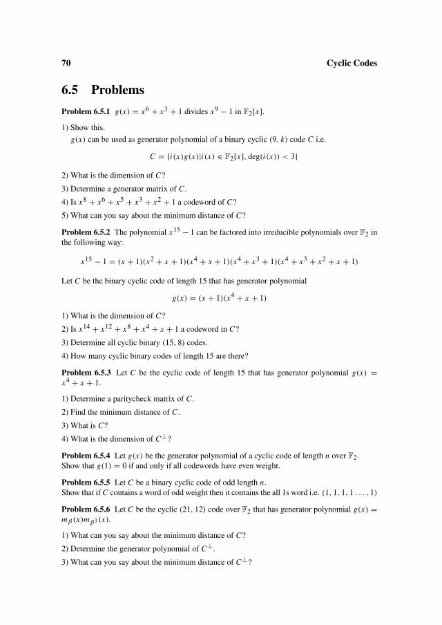
70 Cyclic Codes
6.5 Problems
Problem 6.5.1 g(x) = x6 + x3 + 1 divides x9 − 1 in F2[x].1) Show this.
g(x) can be used as generator polynomial of a binary cyclic (9, k) code C i.e.
C = {i(x)g(x)|i(x) ∈ F2[x], deg(i(x)) < 3}2) What is the dimension of C?
3) Determine a generator matrix of C .
4) Is x8 + x6 + x5 + x3 + x2 + 1 a codeword of C?
5) What can you say about the minimum distance of C?
Problem 6.5.2 The polynomial x15 − 1 can be factored into irreducible polynomials over F2 inthe following way:
x15 − 1 = (x + 1)(x2 + x + 1)(x4 + x + 1)(x4 + x3 + 1)(x4 + x3 + x2 + x + 1)
Let C be the binary cyclic code of length 15 that has generator polynomial
g(x) = (x + 1)(x4 + x + 1)
1) What is the dimension of C?
2) Is x14 + x12 + x8 + x4 + x + 1 a codeword in C?
3) Determine all cyclic binary (15, 8) codes.
4) How many cyclic binary codes of length 15 are there?
Problem 6.5.3 Let C be the cyclic code of length 15 that has generator polynomial g(x) =x4 + x + 1.
1) Determine a paritycheck matrix of C .
2) Find the minimum distance of C .
3) What is C?
4) What is the dimension of C⊥?
Problem 6.5.4 Let g(x) be the generator polynomial of a cyclic code of length n over F2.Show that g(1) = 0 if and only if all codewords have even weight.
Problem 6.5.5 Let C be a binary cyclic code of odd length n.Show that if C contains a word of odd weight then it contains the all 1s word i.e. (1, 1, 1, 1 . . . , 1)
Problem 6.5.6 Let C be the cyclic (21, 12) code over F2 that has generator polynomial g(x) =mβ(x)mβ3 (x).
1) What can you say about the minimum distance of C?
2) Determine the generator polynomial of C⊥.
3) What can you say about the minimum distance of C⊥?

6.5 Problems 71
Problem 6.5.7 Let C be the cyclic code of length 63 over F2 that has generator polynomial(x + 1)(x6 + x + 1)(x6 + x5 + 1).
What can you say about the minimum distance of C ?
Problem 6.5.8
1) Determine a generator polynomial for a cyclic code of length 31 over F2 that can correct 3errors.
2) What is the dimension of the code you found?
3) Can you do better?
Problem 6.5.9 Let C be a binary (n, k) code. Recall that an encoding rule is called systematicif the information (i0, i1, . . . , ik−1) is encoded into a codeword (c0, c1, . . . , cn−1) that contains(i0, i1, . . . , ik−1) in k fixed positions.
A cyclic (n, k) code consists of all the words of the form i(x)g(x) where i(x) has degree < kand g(x) is the generator polynomial of the code.
1) Show that the encoding rule i(x) → i(x)g(x) is not systematic by looking at the (7, 4) codewith generator polynomial x3 + x + 1.We now use the rule i(x) → xn−k i(x) − (xn−k i(x) mod g(x)).
2) Show that xn−k i(x) − (xn−k i(x) mod g(x)) is a codeword in the cyclic code with generatorg(x).
3) Prove that this is a sytematic encoder.
4) Use the same code as above to encode 1011 using the systematic encoder.
Problem 6.5.10 Let C be a cyclic (n, k) code with generator polynomial g(x).
Let h(x) = xn−1g(x)
and let a(x) be a polynomial of degree < k and gcd(h(x), a(x)) = 1.
Let C ′ = {c(x) = i(x)a(x)g(x) mod (xn − 1)| deg(i(x)) < k}.Show that C ′ = C .
Problem 6.5.11 x23 − 1 = (x + 1)mβ(x)mβ5 (x) where mβ(x) = 1 = x11 + x9 + x7 + x6 +x5 + x + 1.
Let C be the (23, 12) code that has generator polynomial mβ(x).
1) Show that C has minimum distance at least 5.
Let Cext be the (24, 12) code obtained by adding an overall parity check.
2) Show that the weights of all the codewords in Cext are divisible by 4.
3) Show that C has minimum distance 7.
4) Show that C is a perfect code.
This is the famous binary Golay code.
Problem 6.5.12 Let C be a cyclic (n, k) code whose generator polynomial g(x) is the productof the different minimalpolynomials of the elements β, β2, β3, . . . , β2t , where β ∈ F2m hasorder n.
We then know that dmin (C) ≥ 2t + 1.
Consider the case where n = a(2t + 1).

72 Cyclic Codes
1) Show that β, β2, β3, . . . , β2t are not zeroes of xa − 1.
2) Show that mβs (x), s = 1, 2, . . . , 2t does not divide xa − 1.
3) Show that gcd(g(x), xa − 1) = 1.
4) Show that p(x) = xn−1xa−1 is a binary polynomial.
5) Show that g(x)|p(x).
6) What is the weight of p(x)?
7) Show that the minimum distance of C is 2t + 1.
Problem 6.5.13 We have
x31 − 1 =(x + 1)(x5 + x2 + 1)(x5 + x3 + 1)(x5 + x4 + x3 + x2 + 1)
(x5 + x3 + x2 + x + 1)(x5 + x4 + x2 + x + 1)(x5 + x4 + x3 + x + 1).
1) How many binary cyclic codes of length 31 are there?
2) Is there one of these with dimension 10 ?
Let C be the code with generator polynomial g(x) = (x + 1)(x5 + x2 + 1).
3) Is x7 + x5 + x4 + x2 + 1 a codeword of C?
4) Is x7 + x5 + x4 + 1 a codeword of C?
5) What can you say about the minimum distance of C?
Problem 6.5.14 Determine the generator polynomials and the dimension of the cyclic codes oflength 63 that corrects 4, 5, 9, 10, 11 and 15 errors.
Problem 6.5.15 Show that there exists cyclic (n, k, dmin ) binary codes with the following pa-rameters:
(21, 12, ≥ 5) , (73, 45, ≥ 10) , (127, 71,≥ 19).
Problem 6.5.16 When we construct binary cyclic codes of length n we use minimal polynomi-als for powers of an element β of order n. It is a natural question if the choice of this element β
is important. This problem treats the question in a special case.
Let n be an odd number and j a number such that gcd(n, j) = 1.
1) Show that the mapping π : {0, 1, . . . , n − 1} → {0, 1, . . . , n − 1} defined by π(x) = x jmod n is a permutation i.e. a bijective mapping.
Let C1 be the cyclic code that has mβ(x) as generator polynomial, and let C2 be the code thathas mβ j (x) as generator polynomial.
2) Show that (c0, c1, . . . , cn−1) ∈ C1 ⇐⇒ (cπ(0), cπ(1), . . . , cπ(n−1)) ∈ C2.
3) What does that mean for the two codes?

Chapter 7
Frames
So far we have considered transmission of independent symbols and block codes. How-ever, in order to assure correct handling and interpretation, the data is usually organizedin files with a certain structure. In a communication system the receiver also needsstructure in order to decode and further process the received sequence correctly. Ageneral discussion of the architecture of communication systems is outside the scopeof this text. However, we can capture some essential aspects of the discussion by as-suming that the information is transmitted in frames of some fixed length. In somepractical systems the frames are already part of the data structure, in other cases thedata is segmented to facilitate the transmission.
It is often desirable to express the performance of the error-correcting code in terms ofthe quality of the frames. We define some commonly used parameters for frame qualityand relate them to the error probability of the codes. If it were possible to constructgood long block codes and decode them with the error probability indicated in Chap-ter 3, the required quality could clearly be reached. However, at this time there is noknown practical method for achieving this performance. Thus we have to study codingmethods that give a satisfactory quality using short codes or simple codes with sub-optimal error-correcting properties. In many cases a combination of two or more cod-ing steps is used, and the combined construction is adapted to the length of the frame.
7.1 Definitions of frames and their efficiency
Definition 7.1.1. A data frame is an entity of data that can be independently stored,communicated, and interpreted. It consists of a header, a data field, and a parity field.
We assume that the data field consists of a fixed number of source symbols, althoughsome systems use frames of variable length identified in the header. When informationis transmitted over a channel, it is encoded using a suitable error-correcting code. Thetransfer frame consists of a fixed number of channel symbols, which in general belongto a different alphabet.
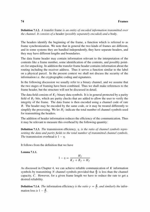
74 Frames
Definition 7.1.2. A transfer frame is an entity of encoded information transmitted overthe channel. It consists of a header (possibly separately encoded) and a body.
The headers identify the beginning of the frame, a function which is referred to asframe synchronization. We note that in general the two kinds of frames are different,and in some systems they are handled independently, they have separate headers, andthey may have different lengths and boundaries.
The data frame header may contain information relevant to the interpretation of thecontents like a frame number, some identification of the contents, and possibly point-ers for unpacking. In addition the transfer frame header contains information about therouting including the receiver address. Thus it serves a function similar to the labelon a physical parcel. In the present context we shall not discuss the security of theinformation i.e. the cryptographic coding and signatures.
In the following discussion we usually refer to a binary channel, and we assume thatthe two stages of framing have been combined. Thus we shall make references to theframe header, but the structure will not be discussed in detail.
The data field consists of K f binary data symbols. It is in general protected by a parityfield of B f bits, which are parity checks that are added to allow the user to verify theintegrity of the frame. The data frame is then encoded using a channel code of rateR. The header may be encoded by the same code, or it may be treated differently tosimplify the processing. We let H f indicate the total number of channel symbols usedfor transmitting the headers.
The addition of header information reduces the efficiency of the communication. Thusit may be relevant to measure this overhead by the following quantity:
Definition 7.1.3. The transmission efficiency, η, is the ratio of channel symbols repre-senting the data and parity fields to the total number of transmitted channel symbols.The transmission overhead is 1 − η.
It follows from the definition that we have
Lemma 7.1.1.
1 − η = H f
K f + B f + H f
As discussed in Chapter 4, we can achieve reliable communication of K informationsymbols by transmitting N channel symbols provided that K
N is less than the channelcapacity, C . However, for a given frame length we have to reduce the rate to get adesired reliability.
Definition 7.1.4. The information efficiency is the ratio γ = RC , and similarly the infor-
mation loss is 1 − RC .

7.1 Definitions of frames and their efficiency 75
In terms of the parameters of the frame we have:
Lemma 7.1.2.
γ = K f(K f + B f
)C
A high efficiency can only be obtained with long frames. The transmission overhead1 − η can be reduced by using a frame that is long compared to the header. We mayassume the length of the header to be almost independent of the frame length, but var-ious practical constraints limit the frame length. Since we assume that the frames areprocessed independently, the length of the frame limits the information efficiency. Wewould get the best reliability by encoding a frame using a good block code of length N ,and when the frame length is given, there is a maximal value of γ that allows a desiredperformance to be reached.
In Example 7.1.1 we demonstrate that at least in principle a small probability of decod-ing failure is possible for a realistic frame size and a low transmission overhead.
Example 7.1.1. Frames on a BSC
If N = 8192 binary symbols and the error probability on the channel is p = 164 , we have on the
average 128 errors. Assuming that the errors are independent, the probability of having j errorsis given by (3.2) or (3.3). If we could use a code to correct 192 errors with bounded distancedecoding, (3.4) gives
Pfail = 5 · 10−8.
From (4.3) we find the capacity of the BSC with p = 1/64 to be C = 0.884. As discussedin relation to Lemma 4.2.2, the Hamming bound is really based on the same calculation as thecapacity. Since we want to correct a fractional number of errors equal to 192
8192 = 3128 , we need a
a code of rate
R ≤ 1 − H
(3
128
)= 0.84
It should be noted that the minimum distance of a code of length 8192 and rate 0.84 is proba-bly only about 194 (by the Gilbert bound, Theorem 1.2.2). However, the following calculationshows that the error probability is not increased much by the low weight codewords. Using theapproximation to the weight distribution (4.7) we find the expected number of codewords ofweight 200 to be about 1012. The contribution to the error probability estimated by the unionbound (3.7) is vanishing. This example shows that for realistic frame sizes we can have a fairlyhigh information efficiency,
γ = 0.84
0.884= 0.95
and still have a low probability of error. However, a block code with these parameters may notbe practical.

76 Frames
7.2 Frame quality
7.2.1 Measures of quality
In a communication network, the transmission of a frame can go wrong in a numberof ways. The address may be corrupted, or the package may be lost or delayed. Itis the purpose of the error-correction to ensure that the frame is delivered to the userwithout errors, or that transmission errors are at least detected. The performance canbe characterized by two numbers:
Definition 7.2.1. The probability of undetected error, P(ue), is the probability that aframe is passed on to the user as error-free while in fact parts of the data are in error.
Definition 7.2.2. The probability of frame error, P(fe), is the probability that the receiverdetects errors in the data, but is not able to correct them, or at least is not able to doso with sufficient reliability.
In some applications the receiver may discard unreliable frames (and the user may beable to have them retransmitted). In other cases it is preferable to get a frame eventhough it is slightly corrupted. In our discussion we shall assume that frames withdetected errors are discarded, and we shall analyze the probability of this event, theprobability of frame error. It should clearly be small enough to allow normal commu-nication to take place, but it does not have to be extremely small (10−5 may be a typicaltarget value). On the other hand the probability of undetected error should be muchsmaller (< 10−10, although for voice communication there is no such requirement).
7.2.2 Parity checks on frames
If there are few errors, it may be sufficient to include a system of parity checks in theframe structure. Often cyclic versions of Hamming codes or subcodes of Hammingcodes are used for this purpose, and we shall discuss only this case.
Lemma 7.2.1. A cyclic binary code defined by the generator polynomial
g(x) = p(x)(x + 1)
where p(x) is a primitive polynomial of degree m has parameters(n, k, d) = (2m − 1, 2m − m − 2, 4)
The maximum number of information symbols is 2m −m−2, but the code can be short-ened by leaving out leading information bits. The m + 1 parity bits are known as theframe check sequence or the CRC (cyclic redundancy check). Usually the frame checksequence is not used for error correction, but errors in the transmission are detected. Ifmore than two errors occur, we may estimate the probability that the frame is acceptedas the probability that a random sequence produces the zero frame check sequence, i.e.
P(ue) ≈ P[t ≥ 2] · 2−m−1 (7.1)
Thus the length of the sequence is chosen to give a sufficient frame length and anacceptable reliability.

7.3 Error detection and error correction 77
Example 7.2.1. Standard CRCs
The following two polynomials used for standard CRCs:
x16 + x12 + x5 + 1
= (x + 1)(x15 + x14 + x13 + x12 + x4 + x3 + x2 + x + 1) CRC-ITU-T
x16 + x15 + x2 + 1 = (x + 1)(x15 + x + 1) CRC-ANSI
Both polynomials are products of x + 1 and irreducible polynomials of degree 15 andperiod 32767. Thus they generate distance 4 subcodes of Hamming codes, and allcombinations of at most three errors in at most 32751 data bits are detected.
7.3 Error detection and error correctionIn this section we discuss the performance of different codes in relation to commu-nication of frames. The discussion also serves as motivation for the various codingstructures introduced in subsequent chapters.
7.3.1 Short block codes
For long frames and channels with a significant error probability, p, we cannot simplyuse a good block code and correct t = N p errors. There is no known method forsolving such a decoding problem with a realistic amount of computation. Thereforewe have to use codes and decoding methods that require less computation. A frame oflength N may be broken into m codewords from a (n, k) code. Here we assume that kis chosen to divide the number of information symbols in the frame.
In Chapter 3 we presented bounds on the error probability for block codes. Assumethat based on a bound or on simulations of the particular code we know the probabilityof decoding error, P(e).
Lemma 7.3.1. If the frame consists of Nn blocks, and the noise is independent, the prob-
ability of a correct frame is
1 − P(ue) = (1 − P(e)
) Nn (7.2)
Thus we can get a very small probability of undetected errors only if the error rate onthe channel is very small, and the system is not very efficient. In order to improve theperformance we may restrict the number of errors corrected in each block. However,with a probability of decoding failure, P( f ), we similarly get a bigger probability offrame error.
Lemma 7.3.2. If the frame consists of Nn blocks, and the noise is independent, the prob-
ability of frame error is
P(fe) = 1 − (1 − P( f )
) Nn (7.3)

78 Frames
This may be the best approach if data is transmitted in short frames. If separate en-coding of the header field is used, it may also be preferable to only correct a limitednumber of errors. However, for the situation of main interest here, it is more efficientto combine error correction with a frame check sequence as discussed in the previoussection. By using 16 or 32 bits for this purpose it is possible to make the probabilityof undetected error very small, and we can still use the full power of the short blockcode for error correction. If there are several equally probable transmitted words for aparticular received block, we may choose to leave it as received.
In the degraded frames some blocks are either not decoded or decoded to a wrongword. We may calculate (a close approximation to) the bit error probability by as-suming that the number of bit errors is d
2 for a block that is not decoded and d for awrong word. These bits are equally likely to hit the information symbols and the paritysymbols in the code, so the number should be multiplied by the rate, R. Clearly it isan advantage in this situation that the encoding is systematic, since decoding mightotherwise change more information bits. However, the output bit error probability isnot necessarily a good measure of the quality of the received signal when the errorsare concentrated in a few blocks. For some purposes the bits are going to be used aslarger symbols, and a symbol error probability would be more relevant. If the errorprobability is used for predicting the performance of subsequent stages of processing,a more accurate description of the error statistics is also required (an assumption ofindependent errors might lead to wrong conclusions). Such a description might againbe a symbol error probability of a combination of bit errors and symbol errors.
Example 7.3.1. Frame reliability of block codes
If a (64, 37) block code is used for the frames in Example 7.1.1, each frame contains 128 blocks.It follows from the Hamming bound Theorem 1.3.1, that in most cases it is possible to correct 6errors. Assuming bounded distance decoding with six errors, we find the probability of decodingfailure from (3.4)
Pfail = 8 · 10−5
Thus the average number of blocks decoded to a wrong codeword is 0.01 in each frame. If adecoding error causes 13 bits to be in error, the average bit error probability would be
Pbit = 13 · 0.01
N= 1.6 · 10−5
but that is not a satisfactory level.
We could correct fewer errors in each block and reduce the probability of undetected error. Thereis a (64, 36) code with minimum distance 12, and we might do minimum distance decoding cor-recting five errors. However, in this case the probability of decoding failure may be found from(3.4) to be
Pfail = 5 · 10−4
and Lemma 7.3.2 gives P(fe) = 0.06, which is clearly too high. If we use maximum likelihooddecoding, but apply a 16 bit CRC, the probability of accepting a frame with a false decoding isreduced by a factor of
2−16 = 1.5 · 10−5.

7.3 Error detection and error correction 79
Lemma 7.3.1 gives P(ue) = 0.01, but with the CRC check this is reduced to
P(ue) ≤ 1.5 · 10−7
while the probability of frame error is
P(fe) ≤ 10−2.
The example shows that with a short block code supplemented with a CRC check we can get anacceptable performance, but the rate, 37
64 = 0.58, is not close to capacity.
The decoder must somehow know how to segment the received sequence into blocks inthe correct way. In the setting we consider here, the obvious solution to the problem ofblock synchronization is to partition the frame starting from the sync pattern. However,block codes, and cyclic codes in particular are quite vulnerable to shifts of the symbolsequence within the frame. In addition all linear codes have the undesirable feature thatthe all 0s word appears. For this reason a fixed coset of such a code is sometimes usedrather than the original code. One such method is to add a pseudo random sequence atthe transmitter and the receiver. If the sequence is not a codeword, it may serve to shiftthe code to a suitable coset.
7.3.2 Convolutional codes
Another approach to error correction in long frames is convolutional codes. Here paritychecks are inserted in the transmitted stream following a simple periodic pattern. Theencoded string consists of blocks of length n each representing k information symbols,but (n, k) are usually very small integers, and each information symbol is used in theencoding of M + 1 blocks (M being referred to as the memory of the code).
The theory of convolutional codes and their decoding is developed in Chapters 8 and 9.
We shall adopt the point of view that a convolutional code is a generic structure thatallows the code to be adapted to the frame length in question. Once the frame lengthand the method of ending the encoding are specified, we have a long block code. Theencoding gives a minimum distance, which is independent of the block length, and thusthe error probability is similar to that of a short block code. Although a convolutionalcode is encoded as one long block, a decoding error changes only a limited segment.
7.3.3 Reed-Solomon codes
When coding is used on a channel with a significant bit error probability, most errorsare corrected by a suitably chosen short block code or convolutional code. However, asmentioned earlier, the probability of decoding error may not be acceptable. The prob-ability of undetected errors can be reduced by having a frame check sequence as partof the data.
However, Reed-Solomon codes provide a much more powerful alternative for the par-ity field in the data frame. The data (which often consists of bytes or 16−32 bit words)
80 Frames
is first encoded using a Reed-Solomon code over a big field, most often the field of 8-bit symbols, F28. Such a code allows several errors to be corrected, often 8 or 16, butat the same time the probability of undetected error is low.
The Reed-Solomon codes are used alone on channels with relatively few errors, butthey can also be combined with a binary channel code. Such a two-stage coding sys-tem is called a concatenated code, and these codes are the subject of Chapter 10.
7.3.4 Low density codes and ‘turbo’ codes
In some sense the advantage of all suboptimal code structures is that some of the errorcorrection can be performed on the basis of ‘local’ parity checks involving a small setof symbols. A more direct approach is to select a parity check matrix, which is verysparse; i.e. each row contains only a relatively small number of 1s. Such codes, calledlow-density parity check codes and their decoding, are treated in Chapter13.
So-called ‘turbo’ codes is a related idea based on iteration between two very simpleconvolutional codes. The data frame is first encoded using one encoder, and then thedata are permuted and encoded again. In the decoding the estimated reliabilities ofthe information symbols are exchanged between the two decoders, and the decoding isiterated until they agree. This topic is also treated in Chapter13.
7.4 ProblemsProblem 7.4.1 Consider frames consisting of 32 words of 16 bits. The first word is the frameheader, which combines header information for both the data frame and the transmission frame.There are used 30 words to transmit 11 data bits protected by the (16,11,4) extended Hammingcode. The last word is a parity check on the frame excluding the header (the mod 2 sum of thedata words).
1) Find the transmission efficiency of the frame.
2) The frame is transmitted over a BSC with bit error probability, p = 0.005. Find the informa-tion efficiency.
3) Prove that the last word is also a word in the extended Hamming code.
4) With the given bit error probability, what is the probability that a word
a) Is correct?
b) Contains one error?
c) Contains two errors or another even number, but is not a codeword?
d) Contains an odd number of errors > 1?
e) Is a codeword different from the one sent.
5) The receiver uses the Hamming code to correct an error and detect double errors. If a doubleerror is detected, the parity word at the end of the frame is used to correct it. What is theprobability that
a) The frame is detected in error (parity word not satisfied) or there are two or more doubleerrors?
b) The frame is accepted with errors?
7.4 Problems 81
Problem 7.4.2 Frames are transmitted on a BSC with p = 1128 . The length of the frame is 4096
bits excluding the unencoded header of the transmission frame.
1) What is the capacity of the channel?
2) Is it possible, in principle, to communicate reliably over the channel using codes of rate
a) 1415 ?
b) 1516 ?
3) Assuming a code rate of R = 34 ,
a) How many information bits are transmitted?
b) What is the information efficiency?
4) If a block code of length 256 is used,
a) What is the average number of bit errors in a block?
b) How many errors, T can be corrected (assuming that this number is found from the Ham-ming bound)?
5) If T errors cause a decoding failure and T + 1 errors a decoding error, what are the proba-bilities of these events? The probability distribution for the number of errors is the binomialdistribution, but it may be approximated by the Poisson distribution.
6) If only this code is used, what are the probabilities of frame error and undetected error?
7) A 16 bit CRC is used to reduce the probability of undetected error.
a) Is the sequence long enough?
b) How much is the information efficiency reduced ?

Chapter 8
Convolutional codes
While most results in coding theory are related to block codes, more complex structuresare found in many applications. In this chapter we present the definitions and basicproperties of some types of codes, which are collectively referred to as convolutionalcodes. The common characteristic of these codes is that the block length is variable, of-ten it is matched to the frame length, while the code is defined by a local encoding rule.
Even though convolutional codes and block codes have been studied in parallel forseveral decades, many aspects of convolutional codes are still not well understood, andthere are several approaches to the theory. Thus the present chapter does not followany established standard for terminology and notation.
8.1 Parameters of convolutional codesThroughout this chapter N denotes the length of the encoded frame and R the rate ofthe convolutional code. All codes considered in this chapter are binary.
The essential difference between convolutional codes and block codes is that the framelength is variable and does not directly enter into the definition of the code. The follow-ing sequence of definitions will lead to the definition of a convolutional code as a familyof block codes with the same nonzero segment in the rows of the generator matrix.
Let R = kn where k and n are integers, and let N be a multiple of n. Most of the exam-
ples have R = 12 , since this case is particularly important and in several ways easier to
analyze than other rates.
Definition 8.1.1. A frame input, u, is a binary vector of RN information symbols. Aninformation vector, v(u), is a binary vector of length N, where
v j ={
ui for j = ⌊ iR
⌋0 otherwise
Thus the input bits are distributed evenly through the frame. We refer to these positionsas information positions even though the encoding is not necessarily systematic.
84 Convolutional codes
Definition 8.1.2. A convolutional encoding of the information vector v(u) by a binarygenerating vector, g, where g0 = gm = 1, maps v(u) to the encoded N-vector
y j =m∑
i=0
giv j−i (8.1)
where the sum is modulo 2, N > m, and the indices are interpreted modulo N.
We refer to the composition in (8.1) as a cyclic convolution of v and g, and the termconvolutional code refers to this form of the encoding. It is simple to perform the en-coding as a non-cyclic convolution, and we can make this modification by insertingm R 0s at the end of the frame input. The reduction of the information efficiency issmall when N is much larger than m. In real frames, a known synchronization patternin the header may serve the same function.
The rate is often a ratio between very small integers, R = kn . In this case the encoded
sequence can be segmented into blocks of length n, each containing k informationsymbols and n − k parity symbols. When we write sequences of such blocks, they areseparated by periods in order to simplify the reading.
The encoding rule has been chosen in such a way that a particular information symbolonly affects a short segment of the encoded frame. Later we shall see that an errorsimilarly only affects a short segment of the syndrome.
Example 8.1.1. A rate 12 convolutional code
A code that is often used in examples has R = 12 and g = (11.10.11). A codeword consists
of blocks each of two symbols, where the first can be chosen as an information symbol andthe second as a parity bit. For N = 16 the frame input u = (11001000) is first convertedinto the information vector v = (10.10.00.00.10.00.00.00) and then convolved with g to givey = (11.01.01.11.11.10.11.00).
Lemma 8.1.1. For a given generating vector, g, the convolutional encoding defines alinear (N, K ) block code with dimension K ≤ RN.
Proof. The linearity follows from (8.1), and the dimension is at most equal to thenumber of symbols in u. �It is easy to find examples of generating vectors such that K < RN for some N . How-ever, the discussion below will show that such codes are usually not interesting. Thefollowing definition serves to eliminate this case.
Definition 8.1.3. An encoding with generating sequence, g, and rate, R, is non-cata-strophic if all block codes obtained from the convolutional encoding (8.1) with suffi-ciently large N have dimension K = RN.
The encoding of a convolutional code may be expressed in matrix form. The matrixthat corresponds to the encoding rule has a particular form since only a narrow band ofsymbols can be nonzero.

8.1 Parameters of convolutional codes 85
Definition 8.1.4. The K by N generator matrix for a convolutional code, G(N) is de-fined by
y = uG(N)
where y is the encoded vector defined by (8.1).
Example 8.1.2. (Example 8.1.1 continued)
For the code with R = 12 and g = (11.10.11), the generator matrix G(16) is obtained in the
following way: In the first row of the generator matrix, g is followed by N − 6 zeros. Row 2 andthe following rows are obtained as cyclic shifts of the previous row by two positions.
G =
1 1 1 0 1 1 0 0 0 0 0 0 0 0 0 00 0 1 1 1 0 1 1 0 0 0 0 0 0 0 00 0 0 0 1 1 1 0 1 1 0 0 0 0 0 00 0 0 0 0 0 1 1 1 0 1 1 0 0 0 00 0 0 0 0 0 0 0 1 1 1 0 1 1 0 00 0 0 0 0 0 0 0 0 0 1 1 1 0 1 11 1 0 0 0 0 0 0 0 0 0 0 1 1 1 01 0 1 1 0 0 0 0 0 0 0 0 0 0 1 1
Lemma 8.1.2. A generating sequence is non-catastrophic if and only if there is a lengthL such that an encoded sequence can contain at most L consecutive 0s when the infor-mation vector has at least one 1 for every m bits.
Proof. If there could be an arbitrarily long sequence of 0s, the input could be periodicwith some period N ′. But this would imply that a nonzero vector was encoded as thezero word by the length N ′ code, and thus the rank would be less than RN ′ . If thereis a length N ′ code with dimension less than RN ′, we can find a nonzero input that isencoded as the zero vector. By repeating this input, we can get an arbitrarily long zeroencoded sequence in a long code. �The proof indicates that a catastrophic encoding would have the undesirable propertythat a periodic nonzero input would produce only a finite nonzero encoded segment inthe output sequence. This also implies that two inputs could differ in arbitrarily manypositions while the outputs were the same except for a finite number of symbols. Forlong frames such an encoding would tend to give many errors in the decoded informa-tion symbols (catastrophic error-propagation).
Definition 8.1.5. The integer, M = �R(m + 1)� − 1, is called the memory of the code.
The parameters of a convolutional code are given as (n, k, M). If R = kn and the length
of g, m+1, is (M+1)n, the encoder stores kM input symbols. More generally we have
Lemma 8.1.3. Every encoded symbol depends on at most the previous M + 1 informa-tion symbols (with the indices taken modulo RN).
Proof. In (8.1) y j depends on m + 1 consecutive symbols of v. If the first of theseis the information symbol ui = v j , j = ⌊ i
R
⌋, then uM+i+1 is the symbol v j ′ ,

86 Convolutional codes
j ′ =⌊
i+M+1R
⌋≥ ⌊ i
R
⌋ +⌊
M+1R
⌋≥ j + m + 1. (When A and B are integers and
R < 1,A = �B R� ⇒ ⌊ AR
⌋ ≥ B). Thus it is outside the range of the summation, whichcan therefore include at most M + 1 information symbols. �
Example 8.1.3. (Example 8.1.1 continued)
The code considered earlier has parameters (2, 1, 2). The encoding in the example is readilyseen to be non-catastrophic, since a nonzero input cannot produce two consecutive zero outputblocks. The memory of the code is 2. The (16, 8) block code generated by this matrix hasminimum distance 4, since (10.00.10.00.10.00.10.00) is a codeword. All longer block codesgenerated by g have minimum distance 5.
The encoding rule (8.1) is slightly too restrictive in the general case. The sequence gshould be defined as a periodic function and allowed to alternate between k generatingvectors. Thus there would be k different types of rows in the generator matrix. Suchcodes will be further discussed in Sections 8.3 and 8.5. Note that we do not require kand n to be mutually prime, and we can introduce a longer period by multiplying k andn by the same factor. Thus a (4, 2) code indicates that the rows in the generator matrixof a rate 1
2 code alternates between two different generators.
As discussed in this section, the concept of convolutional codes is closely related toa particular form of the encoding. We may choose to define the code as such in thefollowing (non-standard) way:
Definition 8.1.6. An (n, k, M) convolutional code is the sequence of block codes oflength, N = jn, obtained by the encoding rule of (8.1).
8.2 Tail-biting codes
In our definition of convolutional codes we have used cyclic convolution as the standardencoding rule. When we want to emphasize that a code is defined in this way, in par-ticular if a relatively short frame is considered, we refer to such a code as a tail-bitingcode. This concept provides a particularly smooth transition from block codes to con-volutional codes. Short tail-biting codes are useful as alternative descriptions of someblock codes, and they have the same properties as block codes in general, whereas along tail-biting code is one of several equivalent ways of defining a convolutional code.
Many good codes with small block lengths have generator matrices of this form. Anequivalent form of the generator matrix for a rate 1
2 code can be obtained by collectingthe even numbered columns into a circulant matrix and the odd numbered columns intoa matrix with the same structure. Such codes are sometimes called quasi-cyclic.
Example 8.2.1. A short tail-biting code
A (16, 8, 5) block code may be described as a rate 12 tail-biting code with generator sequence
g = (11.11.00.10). This code has the largest possible minimum distance for a linear (16, 8)code, although there exists a non-linear (16, 8, 6) code. Longer codes with the same generatoralso have minimum distance 5.

8.3 Parity checks and dual codes 87
Example 8.2.2. The form of the generator matrix for tail-biting codes suggests a relation tocyclic codes.
A (15, 5) cyclic code with minimum distance 7 is generated by g(x) = x10 + x8 + x5 + x4 +x2 + x + 1.
In this case a generator matrix may be written taking shifts of the generator by three positions ata time. It can be proved (as discussed in Problem 8.8.5) that longer tail-biting codes generated bythe same generator also have minimum distance 7. Unfortunately this (and other constructionsderived from good block codes) do not produce the best convolutional codes.
8.3 Parity checks and dual codesParity check matrices are of great importance in the analysis of block codes. In thissection we introduce a parallel concept for convolutional codes, although at this pointit is not as widely used. For a given tail-biting code and a fixed length N , we can find aparity check matrix by solving a system of linear equations as discussed in Chapter 1.However, it is a natural requirement that H should have a structure similar to that of G,and in particular the nonzero part of the rows should be independent of N . With thisconstraint the problem becomes more difficult, and in fact it may not be possible to geta parity check matrix that is quite as simple as G.
For non-catastrophic codes of rate R = 12 , the parity check matrix has the same form
as G, and the nonzero sequence h is obtained by simply reversing g. The orthogonalityof G and H follows from the fact that each term in the inner product appears twice.
Example 8.3.1. (Example 8.1.2 continued)
The parity check matrix has rows that are shifts of h = (11.01.11). Thus by letting the first rowrepresent the first parity check involving the first block, H(16) becomes
H =
1 1 0 0 0 0 0 0 0 0 0 0 1 1 0 10 1 1 1 0 0 0 0 0 0 0 0 0 0 1 11 1 0 1 1 1 0 0 0 0 0 0 0 0 0 00 0 1 1 0 1 1 1 0 0 0 0 0 0 0 00 0 0 0 1 1 0 1 1 1 0 0 0 0 0 00 0 0 0 0 0 1 1 0 1 1 1 0 0 0 00 0 0 0 0 0 0 0 1 1 0 1 1 1 0 00 0 0 0 0 0 0 0 0 0 1 1 0 1 1 1
The parity symbol in position j is associated with a row of H that has its last nonzeroentry in position j . Thus the parity symbol is a function of previously received sym-bols.
For codes of other rates we can always find the parity check sequence, h, by solving asystem of linear equations. If we look again at the row of H that has its last nonzeroentry in position j , the last row of G that we have to consider is the one that has itsfirst nonzero symbols in the same block. If M is the memory of the code, the previousM rows may also have nonzero symbols in the same block, and h has to be orthogonalto these rows. It is not clear offhand how long the vector h must be, but whenever we
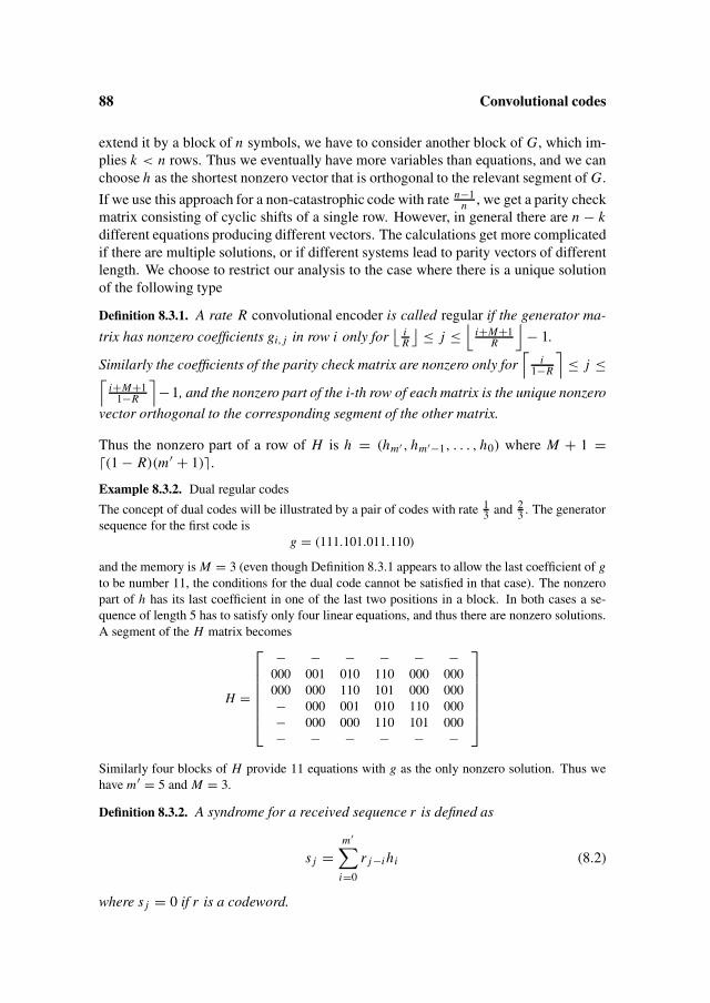
88 Convolutional codes
extend it by a block of n symbols, we have to consider another block of G, which im-plies k < n rows. Thus we eventually have more variables than equations, and we canchoose h as the shortest nonzero vector that is orthogonal to the relevant segment of G.
If we use this approach for a non-catastrophic code with rate n−1n , we get a parity check
matrix consisting of cyclic shifts of a single row. However, in general there are n − kdifferent equations producing different vectors. The calculations get more complicatedif there are multiple solutions, or if different systems lead to parity vectors of differentlength. We choose to restrict our analysis to the case where there is a unique solutionof the following type
Definition 8.3.1. A rate R convolutional encoder is called regular if the generator ma-
trix has nonzero coefficients gi, j in row i only for⌊ i
R
⌋ ≤ j ≤⌊
i+M+1R
⌋− 1.
Similarly the coefficients of the parity check matrix are nonzero only for⌈
i1−R
⌉≤ j ≤⌈
i+M+11−R
⌉−1, and the nonzero part of the i-th row of each matrix is the unique nonzero
vector orthogonal to the corresponding segment of the other matrix.
Thus the nonzero part of a row of H is h = (hm′ , hm′−1, . . . , h0) where M + 1 =�(1 − R)(m′ + 1)�.
Example 8.3.2. Dual regular codes
The concept of dual codes will be illustrated by a pair of codes with rate 13 and 2
3 . The generatorsequence for the first code is
g = (111.101.011.110)
and the memory is M = 3 (even though Definition 8.3.1 appears to allow the last coefficient of gto be number 11, the conditions for the dual code cannot be satisfied in that case). The nonzeropart of h has its last coefficient in one of the last two positions in a block. In both cases a se-quence of length 5 has to satisfy only four linear equations, and thus there are nonzero solutions.A segment of the H matrix becomes
H =
− − − − − −000 001 010 110 000 000000 000 110 101 000 000− 000 001 010 110 000− 000 000 110 101 000− − − − − −
Similarly four blocks of H provide 11 equations with g as the only nonzero solution. Thus wehave m′ = 5 and M = 3.
Definition 8.3.2. A syndrome for a received sequence r is defined as
s j =m′∑
i=0
r j−i hi (8.2)
where s j = 0 if r is a codeword.
8.4 Distances of convolutional codes 89
Lemma 8.3.1. A single error affects at most M + 1 syndrome bits.
We may use H as the generator matrix for a dual rate 1n code, but it is preferable to
define the dual convolutional code by the matrix that has the order of the blocks re-versed (a similar convention is used for cyclic block codes as discussed in Section 6.2).It follows from the definition of regular codes that the dual pair has the same memory.
Lemma 8.3.2. A pair of dual regular codes have the same memory.
8.4 Distances of convolutional codesFor block codes the Hamming distance between codewords gives important informa-tion about the error-correcting properties. In particular the minimum distance is impor-tant. We present a similar parameter for convolutional codes.
If we eliminate the last M bits of the frame input u (or force them to be zero), theencoding (8.1) becomes a regular non-cyclic convolution. This way of adapting theconvolutional encoding to a particular frame length is called termination.
Definition 8.4.1. A terminated (n, k, M) convolutional code is the sequence of blockcodes of length N = jn obtained by the encoding rule (8.1) with the last M input bitsset to zero.
Thus a terminated code has rate less than R, but for a long frame the difference issmall. However, in the analysis of convolutional codes it is also useful to considershort terminated codes. If we consider j consecutive rows of the generator matrix andthe segment of the encoded sequence where these rows are not all zero, the length N ′of the sequence satisfies j = ⌊
R(N ′ − m)⌋
. The set of encoded sequences is a linear(N ′, j) code called the j-th terminated code.
Definition 8.4.2. The j -th row distance of the convolutional code is the minimum weightof a nonzero vector spanned by j consecutive rows.
Thus the j -th row distance is the minimum distance of the j -th terminated code. Sinceeach terminated code contains all shorter codes, we have
Lemma 8.4.1. The row distance is a decreasing function of j .
Definition 8.4.3. The free distance, d f , is the minimum value of the row distance.
In most codes of interest the row distance is constant from j = 1, or it is reached with avery small value of j . The free distance d f is also the minimum distance of the convo-lutional code as defined in Definition 8.1.2 and Lemma 8.1.1 for any sufficiently largeN . The free distance is the most important measure of the error-correcting capabilityof a convolutional code.
Lemma 8.4.2. For a given non-catastrophic convolutional code, all tail-biting codes oflength greater than some constant N ′ have minimum distance d f .

90 Convolutional codes
Proof. Since the long tail-biting codes contain all shorter terminated codes, they havewords of weight d f . A codeword that is not contained in a terminated code is producedby a nonzero input in the full length of the code. However, for a non-catastrophic codesuch a codeword cannot have arbitrarily long zero segments, and thus the weight mustincrease with the length of the code. For sufficiently long codes, the weights of thesecodewords must exceed d f . �
Theorem 8.4.1. A convolutional code with free distance d f can correct any error pat-
tern of weight less thand f2 if N is sufficiently large.
Proof. The theorem follows from Lemma 8.4.1 and a similar result for block codes. �Lemma 8.4.1 provides a link between the free distance of convolutional codes and theminimum distance of tail-biting codes. However, the following result is more usefulfor predicting possible values of d f .
Theorem 8.4.2. The free distance of a convolutional code is upper bounded by the min-imum distance of the best (N ′, j) block code, where j = �R(N ′ − m)�.
Proof. The terminated code is a block code with these parameters, and its minimumdistance, the row distance, is an upper bound on the free distance of the convolutionalcode. �Since the largest value of the minimum distance of any block code with given param-eters is known for a large number of cases, it is possible to obtain close bounds on thefree distance. In spite of this important connection between the minimum distances,the result does not suggest any constructions.
Example 8.4.1. We may obtain an upper bound on the distance of a (3, 1) code with M = 3by considering the parameters of block codes obtained by termination: (11, 1), (14, 2), (17, 3),. . . . It follows that the upper bound is 9. For rate 2
3 we should compare with block codes(7, 2), (10, 4), (13, 6), . . . , and the upper bound is 4.
In this section we have shown that convolutional codes have a parameter, the free dis-tance, which is closely related to minimum distances of block codes. However, as Nincreases, this distance is fixed. Thus while it is useful to know that even in short seg-ments, all error patterns of weight less than
d f2 can be corrected, we need to know how
the number of errors can be increased for long segments. We return to this problem inChapter 9.
8.5 Punctured codesIn Problem 1.5.10 we have considered two methods for decreasing the length of a blockcode by one symbol. We give the definition here to emphasize the terminology.
Definition 8.5.1. A code is shortened when an information symbol is first forced to bezero and then eliminated. A code is punctured when a parity symbol is eliminated.
8.6 Linear systems as encoders 91
Thus the rate is decreased by shortening and increased by puncturing the code. Theopposite operations are called lengthening and extending. We have
Lemma 8.5.1. The dual of a shortened code is the punctured dual code.
Proof. The dual of the original code has a parity symbol where the original code has aninformation symbol. If this symbol is forced to be zero, the remaining positions satisfyall the parity checks, and the position can be punctured. �These concepts may be applied to convolutional codes, but usually symbols are punc-tured in a periodic pattern through the entire frame or a predefined part of the frame.The main advantage of puncturing is that the rate of the code can be increased whilethe structure of the decoder is unchanged. In particular the same decoder can be used.We return to this aspect in Chapter 9.
Most of the high-rate codes that are used in current systems are obtained by puncturingcodes of rate 1
2 . Puncturing may be used to change between different rates depend-ing on the bit error probability, or the technique may be used to vary the number ofcorrectable errors so that some information symbols are given additional protection.
The definition of general (n, k, M) codes in Section 8.1 was partially motivated by thestructure of punctured codes.
Example 8.5.1. Starting from the rate 12 code in Example 8.1.1, we can puncture every other
parity symbol to get a rate 23 code with generators g′ = (1101) and g′′ = (11111). We still
have M = 2. In order to find the generator of the dual code we can solve a system of linearequations or we can shorten the dual code by eliminating the same symbols. Before we caneliminate the symbols from the dual code, we must find a linear combination of rows such thatall the relevant symbols are zero. In this case it is simply the sum of three consecutive shifts ofh, h′ = (111.011.110). However when this generator is interpreted as generating a code of rate13 , the memory is still 2.
8.6 Linear systems as encodersConvolutional codes have been characterized by the parameters, (n, k, M). The linearencoding rule can be expressed in matrix form by the convolution
y j =∑i≥0
Gi u j−i (8.3)
Here the input blocks, u, have length k, the output blocks, y, length n, and the matrices,Gi , are k by n. Note that for k = 1, (8.3) coincides with (8.1), but if k is not very small,this is a much wider definition of encoding rules than (8.1).
The encoding equation suggests using methods from linear systems or power series,and in particular the technique of generating functions (Z -transforms). This allows usto express the code by a polynomial generating function
y(D) = u(D)G(D) (8.4)
The indeterminate, D, is used in the literature, and it may be thought of as an elementin an extension field of the symbol field (as Z is complex in usual linear systems).
92 Convolutional codes
The D notation allows us to manipulate sequences in a more compact notation, but themost important difference is that we can write infinite (eventually periodic) sequencesas rational functions. The notation is used to study questions relating to encoders,notably equivalences between encoders and duality of encoders. Since we assumeda finite memory in (8.1), the entries in G(D) will be polynomials of degree at mostm. However by suitable scalings and row operations we can obtain a generator matrixin systematic form, i.e. a form containing a k by k identity matrix while the remain-ing entries may be rational functions in D. Such systematic encoders are sometimespreferred.
Example 8.6.1. (Example 8.1.1 continued)
We may write the generator and parity check matrices as
G(D) = (1 + D + D2, 1 + D2) H(D) = (1 + D2, 1 + D + D2)
Note that the polynomial vectors are orthogonal, but to convert them to binary vectors, the sym-bol D in H must be interpreted as a left shift of one block.
Example 8.6.2. (Example 8.3.2 continued)
The generator matrix for a rate 13 code may be written in transform notation as
G(D) = (1 + D + D3, 1 + D2 + D3, 1 + D + D2)
Similarly we may take the transform of the generator matrix (parity check matrix), but in orderto get the same result of polynomial multiplication and scalar products of vectors, we need touse negative powers of D or reverse the order of the blocks:
H(D) =[
1 1 + D D2
1 + D D 1
]
The encoding rules for convolutional codes are often non-systematic. The generatormatrix for any particular tail-biting code could be converted to systematic form, but thestructure would be changed. The D notation allows us to reduce the generator matrixto systematic form if rational functions are allowed for the parity symbols.
Example 8.6.3. (Example 8.3.2 continued)
The generator matrix
G(D) = (1 + D + D3, 1 + D2 + D3, 1 + D + D2)
can be replaced by the systematic encoding matrix
Gs(D) =(
1,1 + D2 + D3
1 + D + D3,
1 + D + D2
1 + D + D3
)
If H is seen as the generator matrix for the dual rate 23 code, we can similarly modify the encod-
ing to make it systematic:
Hs (D) = 1 0 1+D+D3
1+D+D2
0 1 1+D2+D3
1+D+D2
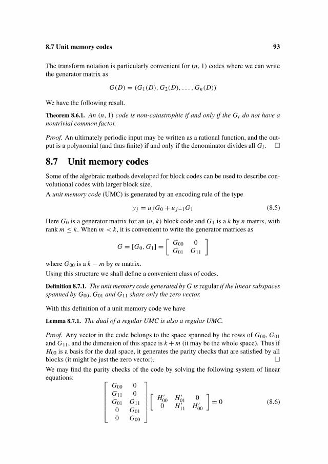
8.7 Unit memory codes 93
The transform notation is particularly convenient for (n, 1) codes where we can writethe generator matrix as
G(D) = (G1(D), G2(D), . . . , Gn(D))
We have the following result.
Theorem 8.6.1. An (n, 1) code is non-catastrophic if and only if the Gi do not have anontrivial common factor.
Proof. An ultimately periodic input may be written as a rational function, and the out-put is a polynomial (and thus finite) if and only if the denominator divides all Gi . �
8.7 Unit memory codesSome of the algebraic methods developed for block codes can be used to describe con-volutional codes with larger block size.
A unit memory code (UMC) is generated by an encoding rule of the type
y j = u j G0 + u j−1G1 (8.5)
Here G0 is a generator matrix for an (n, k) block code and G1 is a k by n matrix, withrank m ≤ k. When m < k, it is convenient to write the generator matrices as
G = [G0, G1] =[
G00 0G01 G11
]
where G00 is a k − m by m matrix.
Using this structure we shall define a convenient class of codes.
Definition 8.7.1. The unit memory code generated by G is regular if the linear subspacesspanned by G00, G01 and G11 share only the zero vector.
With this definition of a unit memory code we have
Lemma 8.7.1. The dual of a regular UMC is also a regular UMC.
Proof. Any vector in the code belongs to the space spanned by the rows of G00, G01and G11, and the dimension of this space is k + m (it may be the whole space). Thus ifH00 is a basis for the dual space, it generates the parity checks that are satisfied by allblocks (it might be just the zero vector). �We may find the parity checks of the code by solving the following system of linearequations:
G00 0G11 0G01 G11
0 G010 G00
[H ′
00 H ′01 0
0 H ′11 H ′
00
]= 0 (8.6)
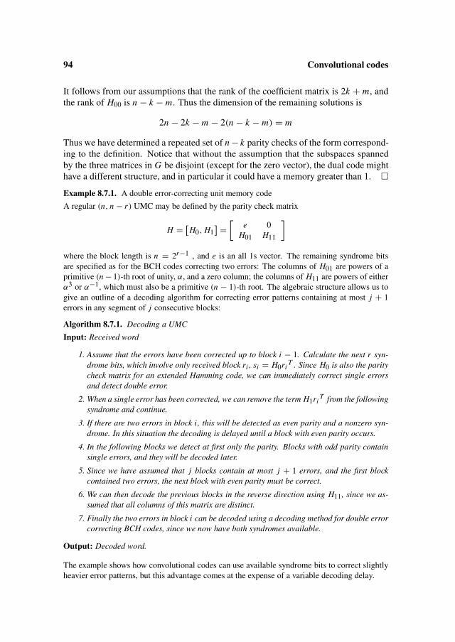
94 Convolutional codes
It follows from our assumptions that the rank of the coefficient matrix is 2k + m, andthe rank of H00 is n − k − m. Thus the dimension of the remaining solutions is
2n − 2k − m − 2(n − k − m) = m
Thus we have determined a repeated set of n − k parity checks of the form correspond-ing to the definition. Notice that without the assumption that the subspaces spannedby the three matrices in G be disjoint (except for the zero vector), the dual code mighthave a different structure, and in particular it could have a memory greater than 1. �Example 8.7.1. A double error-correcting unit memory code
A regular (n, n − r) UMC may be defined by the parity check matrix
H = [H0, H1
] =[
e 0H01 H11
]
where the block length is n = 2r−1 , and e is an all 1s vector. The remaining syndrome bitsare specified as for the BCH codes correcting two errors: The columns of H01 are powers of aprimitive (n − 1)-th root of unity, α, and a zero column; the columns of H11 are powers of eitherα3 or α−1, which must also be a primitive (n − 1)-th root. The algebraic structure allows us togive an outline of a decoding algorithm for correcting error patterns containing at most j + 1errors in any segment of j consecutive blocks:
Algorithm 8.7.1. Decoding a UMC
Input: Received word
1. Assume that the errors have been corrected up to block i − 1. Calculate the next r syn-drome bits, which involve only received block ri , si = H0ri
T . Since H0 is also the paritycheck matrix for an extended Hamming code, we can immediately correct single errorsand detect double error.
2. When a single error has been corrected, we can remove the term H1riT from the following
syndrome and continue.
3. If there are two errors in block i , this will be detected as even parity and a nonzero syn-drome. In this situation the decoding is delayed until a block with even parity occurs.
4. In the following blocks we detect at first only the parity. Blocks with odd parity containsingle errors, and they will be decoded later.
5. Since we have assumed that j blocks contain at most j + 1 errors, and the first blockcontained two errors, the next block with even parity must be correct.
6. We can then decode the previous blocks in the reverse direction using H11, since we as-sumed that all columns of this matrix are distinct.
7. Finally the two errors in block i can be decoded using a decoding method for double errorcorrecting BCH codes, since we now have both syndromes available.
Output: Decoded word.
The example shows how convolutional codes can use available syndrome bits to correct slightlyheavier error patterns, but this advantage comes at the expense of a variable decoding delay.

8.8 Problems 95
8.8 Problems
Problem 8.8.1 Consider a rate 12 convolutional code with generating vector g = (11.10.01.11).
1) How is the information sequence u = (10111000) encoded?
2) Write a generator matrix for the tail-biting code of length 16. What is the dimension of thecode?
3) How many consecutive zero blocks can there be in a nonzero codeword?
4) Is the encoding non-catastrophic?
5) What is the memory of the code?
6) Find the minimum distance of the code of length 16.
7) What is the minimum distance of a code of length 64?
Problem 8.8.2 A rate 13 convolutional code has generating vector g = (111.101.110).
1) Is the encoding non-catastrophic?
2) What is the memory of the code?
3) Encode the sequence u = (11010).
Problem 8.8.3 Consider the same code as in Problem 8.8.1.
1) Prove that the matrix from 8.8.1 2 is also a parity check matrix for the code.
2) Find the syndrome for a single error.
3) In a long code the syndrome is found to be (. . . 00011000 . . . ). Find a likely error pattern.
4) Same question with the syndrome (. . . 0001000 . . . ).
Problem 8.8.4 Consider the same code as in Problem 8.8.2.
1) Find a parity check matrix for the tail-biting code of length 15.
2) Is the code regular?
Problem 8.8.5 Consider the same codes as in Problems 8.8.1 and 8.8.2.
1) Find the row distances of the codes and their free distances.
2) How many errors can the codes correct?
3) Give examples of patterns with higher weight that lead to decoding error.
Problem 8.8.6 Consider the (2, 1, 3) code from Problem 8.8.1and puncture the code to get arate 2
3 code.
1) Write a generator matrix of length 15 for this code.
2) Find a parity check matrix for the code (or a generator matrix for the dual code).
Problem 8.8.7 Same codes as in Problems 8.8.1 and 8.8.2.
1) Write generator matrices and parity check matrices in D notation.
2) Verify that the rows of these matrices are orthogonal when the terms are multiplied as poly-nomials.

96 Convolutional codes
Problem 8.8.8 Consider the convolutional (2, 1, 4) code with generator matrix
G(D) = [g0(D), g1(D)
] =[1 + D + D4, 1 + D2 + D3 + D4
]
1) Show that g0 is reducible, while g1 factors into two primary polynomials.
2) Show that it follows from 1) that the weight of short encoded sequences is at least 7.
3) For the information sequence u = (1011), find the weight of the encoded sequence.
4) How many consecutive blocks can be 00?
Problem 8.8.9 A convolutional (2, 1, 6) code which is often used has generator matrix
G(D) = [g0(D), g1(D)
] =[1 + D + D2 + D5 + D6, 1 + D2 + D3 + D4 + D6
]
The free distance is 10.
1) Show that g0 is irreducible, while g1 factors into two binary polynomials.
2) Find the information polynomial, u(D), of lowest degree such that for some j ,
u(D)g1(D) = 1 + D j
3) Find the weight of the encoded sequence for this information polynomial.
Problem 8.8.10 Let g be the generating vector for a non-catastrophic R = 12 encoding.
1) Is it possible to get the same code with a different vector ?
2) Write G as a polynomial, G(D). Is G(D)(1 + D2) a generating vector for a non-catastrophicencoding ?
3) Prove that the encoding is non-catastrophic if and only if g(x) does not have a factor that is apolynomial in D2.
Problem 8.8.11 Consider the (8, 4) unit memory code generated by the matrix:
G =[
e 0G0 G1
]
where
G0 =
0 1 0 0 1 0 1 10 0 1 0 1 1 1 00 0 0 1 0 1 1 1
, G1 =
0 1 1 1 0 1 0 00 0 1 0 0 1 1 10 0 0 1 1 1 0 1
and e is a vector of 1s.
1) Show that the code is regular.
2) Verify that the dual code has the same form.
3) Verify that the code is constructed as discussed in Example 8.6.1.
4) Find the free distance.

Chapter 9
Maximum likelihood decodingof convolutional codes
The main topic of this chapter is an efficient algorithm for ML decoding of convolu-tional codes. The algorithm is described in detail in Section 9.2, but before we presentit we need a new way of describing convolutional codes.
9.1 Finite state descriptions of convolutional codesIn this section we describe convolutional codes as output sequences of finite state ma-chines.
Definition 9.1.1. A finite state machine is defined by a finite set of states,
� = {σ0, σ1, σ2, . . . , σr },an input alphabet A, a next state function from A × � to �, an output alphabet B, andan output function from A × � to B. In any instance of time, j, the machine receivesan input symbol, makes a transition from its current state to the state given by the nextstate function and produces the output symbol given by the output function.
The encoding of a convolutional code may be described by a finite state machine (theencoder). The input is an information symbol, u j . It is usually most convenient toidentify the state by the previous M input symbols, [u j−1, u j−2, . . . , u j−M ], and weshall refer to state σi as the state where the previous input bits are the binary expansionof the integer i with the most recent symbol as the least significant bit.
The next state is obtained by shifting the state variables to the right and adding the newinput as the first state variable. Thus a transition from state i leads to either state 2i or2i + 1. An important consequence of this labeling of the states is that all encoders witha given memory have the same states and next state mapping.
The output, y j , is a string of symbols, which are determined as a function of the inputand the state, i.e. of M + 1 input symbols. For a linear code, the output function may
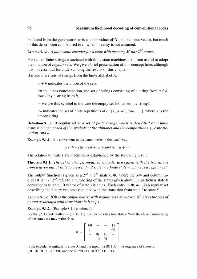
98 Maximum likelihood decoding of convolutional codes
be found from the generator matrix as the product of G and the input vector, but muchof this description can be used even when linearity is not assumed.
Lemma 9.1.1. A finite state encoder for a code with memory M has 2M states.
For sets of finite strings associated with finite state machines it is often useful to adoptthe notation of regular sets. We give a brief presentation of this concept here, althoughit is not essential for understanding the results of this chapter.
If a and b are sets of strings from the finite alphabet A,
a + b indicates the union of the sets,
ab indicates concatenation, the set of strings consisting of a string from a fol-lowed by a string from b,
− we use this symbol to indicate the empty set (not an empty string),
a∗ indicates the set of finite repetitions of a: {λ, a, aa, aaa, . . .}, where λ is theempty string.
Definition 9.1.2. A regular set is a set of finite strings which is described by a finiteexpression composed of the symbols of the alphabet and the compositions +, concate-nation, and ∗.
Example 9.1.1. It is convenient to use parentheses in the usual way
a ∗ (b + c)d = bd + cd + abd + acd + · · ·The relation to finite state machines is established by the following result.
Theorem 9.1.1. The set of strings, inputs or outputs, associated with the transitionsfrom a given initial state to a given final state in a finite state machine is a regular set.
The output function is given as a 2M × 2M matrix, , where the row and column in-dices 0 ≤ i < 2M refer to a numbering of the states given above. In particular state 0corresponds to an all 0 vector of state variables. Each entry in , φi ′ i , is a regular setdescribing the binary vectors associated with the transition from state i to state i ′.Lemma 9.1.2. If is the output matrix with regular sets as entries, b gives the sets ofoutput associated with transitions in b steps.
Example 9.1.2. (Example 8.1.1 continued)
For the (2, 1) code with g = (11.10.11), the encoder has four states. With the chosen numberingof the states we may write as
=
00 − − 1111 − − 00− 01 10 −− 10 01 −
If the encoder is initially in state 00 and the input is (101100), the sequence of states is(01, 10, 01, 11, 10, 00) and the output (11.10.00.01.01.11).
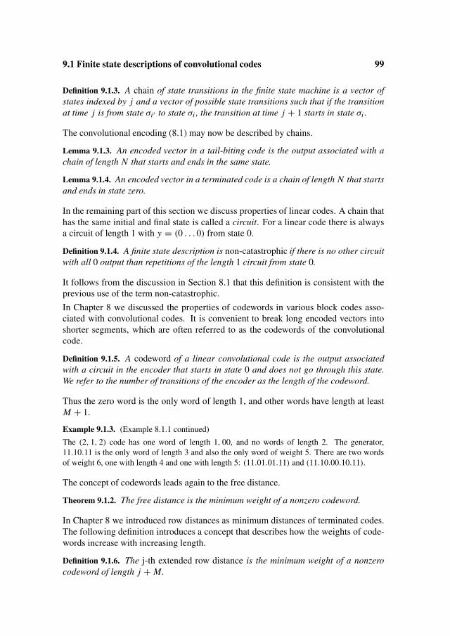
9.1 Finite state descriptions of convolutional codes 99
Definition 9.1.3. A chain of state transitions in the finite state machine is a vector ofstates indexed by j and a vector of possible state transitions such that if the transitionat time j is from state σi ′ to state σi , the transition at time j + 1 starts in state σi .
The convolutional encoding (8.1) may now be described by chains.
Lemma 9.1.3. An encoded vector in a tail-biting code is the output associated with achain of length N that starts and ends in the same state.
Lemma 9.1.4. An encoded vector in a terminated code is a chain of length N that startsand ends in state zero.
In the remaining part of this section we discuss properties of linear codes. A chain thathas the same initial and final state is called a circuit. For a linear code there is alwaysa circuit of length 1 with y = (0 . . . 0) from state 0.
Definition 9.1.4. A finite state description is non-catastrophic if there is no other circuitwith all 0 output than repetitions of the length 1 circuit from state 0.
It follows from the discussion in Section 8.1 that this definition is consistent with theprevious use of the term non-catastrophic.
In Chapter 8 we discussed the properties of codewords in various block codes asso-ciated with convolutional codes. It is convenient to break long encoded vectors intoshorter segments, which are often referred to as the codewords of the convolutionalcode.
Definition 9.1.5. A codeword of a linear convolutional code is the output associatedwith a circuit in the encoder that starts in state 0 and does not go through this state.We refer to the number of transitions of the encoder as the length of the codeword.
Thus the zero word is the only word of length 1, and other words have length at leastM + 1.
Example 9.1.3. (Example 8.1.1 continued)
The (2, 1, 2) code has one word of length 1, 00, and no words of length 2. The generator,11.10.11 is the only word of length 3 and also the only word of weight 5. There are two wordsof weight 6, one with length 4 and one with length 5: (11.01.01.11) and (11.10.00.10.11).
The concept of codewords leads again to the free distance.
Theorem 9.1.2. The free distance is the minimum weight of a nonzero codeword.
In Chapter 8 we introduced row distances as minimum distances of terminated codes.The following definition introduces a concept that describes how the weights of code-words increase with increasing length.
Definition 9.1.6. The j-th extended row distance is the minimum weight of a nonzerocodeword of length j + M.
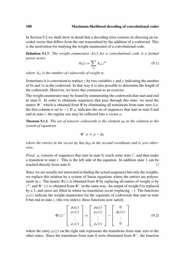
100 Maximum likelihood decoding of convolutional codes
In Section 9.2 we shall show in detail that a decoding error consists in choosing an en-coded vector that differs from the one transmitted by the addition of a codeword. Thisis the motivation for studying the weight enumerator of a convolutional code.
Definition 9.1.7. The weight enumerator A(z) for a convolutional code is a formalpower series
A(z) =∑w
Awzw (9.1)
where Aw is the number of codewords of weight w.
Sometimes it is convenient to replace z by two variables x and y indicating the numberof 0s and 1s in the codeword. In that way it is also possible to determine the length ofthe codewords. However, we leave this extension as an exercise.
The weight enumerator may be found by enumerating the codewords that start and endin state 0. In order to eliminate sequences that pass through this state, we need thematrix − which is obtained from by eliminating all transitions from state zero (i.e.the first column is set to −). If ρi indicates the set of sequences that start in state 0 andend in state i , the regular sets may be collected into a vector ρ.
Theorem 9.1.3. The set of nonzero codewords is the element ρ0 in the solution to thesystem of equations
−ρ = ρ − φ1
where the entries in the vector φ1 has φ10 in the second coordinate and is zero other-wise.
Proof. ρi consists of sequences that start in state 0, reach some state i ′, and then makea transition to state i . This is the left side of the equation. In addition state 1 can bereached directly from state 0. �
Since we are usually not interested in finding the actual sequences but only the weights,we replace this relation by a system of linear equations where the entries are polyno-mials in z. The matrix (z) is obtained from by replacing all entries of weight w byzw, and −(z) is obtained from − in the same way. An output of weight 0 is replacedby a 1, and zeros are filled in where no transitions occur (replacing −). The functionsρi (z) indicate the weight enumerator for the segments of codewords that start in state0 but end in state i , (the row index); these functions now satisfy
(z)−
ρ0(z)ρ1(z)
...
ρr (z)
=
ρ0(z)ρ1(z)
...
ρr (z)
−
0φ1(z)
...
0
(9.2)
where the entry ρi (z) on the right side represents the transitions from state zero to theother states. Since the transitions from state 0 were eliminated from −, the function

9.1 Finite state descriptions of convolutional codes 101
ρ0 enumerates the chains that end here, which are the codewords. Thus we can findA(z) = ρ0(z) by solving a system of symbolic equations. With a suitable programmingtool that can be done even for a moderately large number of states. It follows from thiscalculation that we have
Theorem 9.1.4. The weight enumerator of a convolutional code is the rational functionρ0(z).
Example 9.1.4. (Example 8.1.1 continued)
The codewords of the code from Example 8.1.1 may be found by removing the zero circuit oflength 1. This gives the following system of equations:
0 0 0 z2
0 0 0 10 z z 00 z z 0
ρ0ρ1ρ2ρ3
=
ρ0ρ1 − z2
ρ2ρ3
And we obtain the weight enumerator as
A(z) = ρ0(z) = z5
1 − 2z= z5 + 2z6 + 4z7 + · · ·
The weight enumerator is primarily of interest as a tool for obtaining upper boundson the error probability. By following the derivation of the union bound in Chapter 3,we get an upper bound on the probability that the decoder makes an error in the firstblock. Assume that the zero word is transmitted. An ML decoder will select one ofthe nonzero words leaving state 0 in the first block, and this will happen if the receivedsequence is closer to one of these words than to the zero sequence. Thus the samecalculation as the one used to derive (3.7) gives
P(e) <∑w>0
∑j≥ w
2
Aw
(w
j
)p j (1 − p)w− j (9.3)
which may be approximated by
P(e) <1
2A(Z) (9.4)
where Z is the function
Z = √4 p(1 − p)
The bound (9.3) is closely related to (3.9) in Chapter 3, but it is particularly useful forconvolutional code since it allows us to use the rational form of the weight enumerator.

102 Maximum likelihood decoding of convolutional codes
9.2 Maximum likelihood decoding
The process of decoding a convolutional code is conveniently described as a search fora chain that disagrees with the received sequence in the smallest number of positions.We present several properties of maximum likelihood decoding which lead to the im-portant Viterbi decoding algorithm for convolutional codes (we use this name althoughthe algorithm may be seen as a special case of the principle of dynamic programming).
Earlier we introduced the transition matrix with entries φi ′ i , which are the blocksthat the encoder outputs in making a transition from state i to state i ′. For a receivedblock, r , we may find the number of differences between φi ′ i and r j as
ei ′ i ( j) = W(φi ′ i + r j
)
where W indicates Hamming weight. Thus we may store these values in a table indexedby the values of r .
Example 9.2.1. Consider the decoding of the (3, 1) code with M = 3 and
g = (111.011.110.111)
The encoder has memory 3 and eight states. The state transition matrix is
=
000 − − − 111 − − −111 − − − 000 − − −− 011 − − − 100 − −− 100 − − − 011 − −− − 110 − − − 001 −− − 001 − − − 110 −− − − 101 − − − 010− − − 010 − − − 101
For a received zero block, the ei ′ i are found as the number of 1s in each entry of this matrix. Werefer to this integer matrix as E000. Similarly for each of the other seven values of a receivedblock we need a table of the corresponding error weights. For 101 we have
E101 =
2 − − − 1 − − −1 − − − 2 − − −− 2 − − − 1 − −− 1 − − − 2 − −− − 2 − − − 1 −− − 1 − − − 2 −− − − 0 − − − 3− − − 3 − − − 0
Here the symbol ‘–’ is used instead of ∞ (or a sufficiently large number).
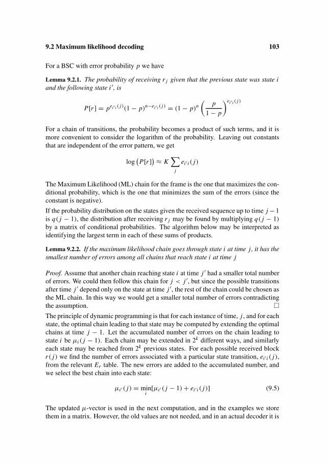
9.2 Maximum likelihood decoding 103
For a BSC with error probability p we have
Lemma 9.2.1. The probability of receiving r j given that the previous state was state iand the following state i ′, is
P[r ] = pei′ i ( j )(1 − p)n−ei′ i ( j ) = (1 − p)n(
p
1 − p
)ei′ i ( j )
For a chain of transitions, the probability becomes a product of such terms, and it ismore convenient to consider the logarithm of the probability. Leaving out constantsthat are independent of the error pattern, we get
log(P[r ]) ≈ K
∑j
ei ′ i ( j)
The Maximum Likelihood (ML) chain for the frame is the one that maximizes the con-ditional probability, which is the one that minimizes the sum of the errors (since theconstant is negative).
If the probability distribution on the states given the received sequence up to time j −1is q( j − 1), the distribution after receiving r j may be found by multiplying q( j − 1)
by a matrix of conditional probabilities. The algorithm below may be interpreted asidentifying the largest term in each of these sums of products.
Lemma 9.2.2. If the maximum likelihood chain goes through state i at time j , it has thesmallest number of errors among all chains that reach state i at time j
Proof. Assume that another chain reaching state i at time j ′ had a smaller total numberof errors. We could then follow this chain for j < j ′, but since the possible transitionsafter time j ′ depend only on the state at time j ′, the rest of the chain could be chosen asthe ML chain. In this way we would get a smaller total number of errors contradictingthe assumption. �The principle of dynamic programming is that for each instance of time, j , and for eachstate, the optimal chain leading to that state may be computed by extending the optimalchains at time j − 1. Let the accumulated number of errors on the chain leading tostate i be µi ( j − 1). Each chain may be extended in 2k different ways, and similarlyeach state may be reached from 2k previous states. For each possible received blockr( j) we find the number of errors associated with a particular state transition, ei ′i ( j),from the relevant Er table. The new errors are added to the accumulated number, andwe select the best chain into each state:
µi ′ ( j) = mini
[µi ′ ( j − 1) + ei ′ i ( j)] (9.5)
The updated µ-vector is used in the next computation, and in the examples we storethem in a matrix. However, the old values are not needed, and in an actual decoder it is
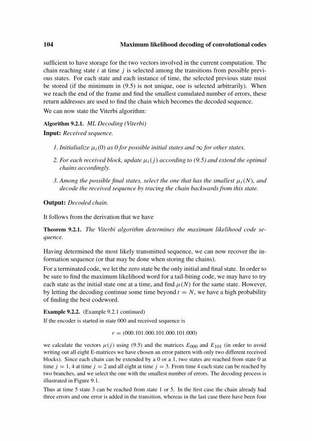
104 Maximum likelihood decoding of convolutional codes
sufficient to have storage for the two vectors involved in the current computation. Thechain reaching state i at time j is selected among the transitions from possible previ-ous states. For each state and each instance of time, the selected previous state mustbe stored (if the minimum in (9.5) is not unique, one is selected arbitrarily). Whenwe reach the end of the frame and find the smallest cumulated number of errors, thesereturn addresses are used to find the chain which becomes the decoded sequence.
We can now state the Viterbi algorithm:
Algorithm 9.2.1. ML Decoding (Viterbi)
Input: Received sequence.
1. Initialialize µi (0) as 0 for possible initial states and ∞ for other states.
2. For each received block, update µi ( j) according to (9.5) and extend the optimalchains accordingly.
3. Among the possible final states, select the one that has the smallest µi (N), anddecode the received sequence by tracing the chain backwards from this state.
Output: Decoded chain.
It follows from the derivation that we have
Theorem 9.2.1. The Viterbi algorithm determines the maximum likelihood code se-quence.
Having determined the most likely transmitted sequence, we can now recover the in-formation sequence (or that may be done when storing the chains).
For a terminated code, we let the zero state be the only initial and final state. In order tobe sure to find the maximum likelihood word for a tail-biting code, we may have to tryeach state as the initial state one at a time, and find µ(N) for the same state. However,by letting the decoding continue some time beyond t = N , we have a high probabilityof finding the best codeword.
Example 9.2.2. (Example 9.2.1 continued)
If the encoder is started in state 000 and received sequence is
r = (000.101.000.101.000.101.000)
we calculate the vectors µ( j) using (9.5) and the matrices E000 and E101 (in order to avoidwriting out all eight E-matrices we have chosen an error pattern with only two different receivedblocks). Since each chain can be extended by a 0 or a 1, two states are reached from state 0 attime j = 1, 4 at time j = 2 and all eight at time j = 3. From time 4 each state can be reached bytwo branches, and we select the one with the smallest number of errors. The decoding process isillustrated in Figure 9.1.
Thus at time 5 state 3 can be reached from state 1 or 5. In the first case the chain already hadthree errors and one error is added in the transition, whereas in the last case there have been four
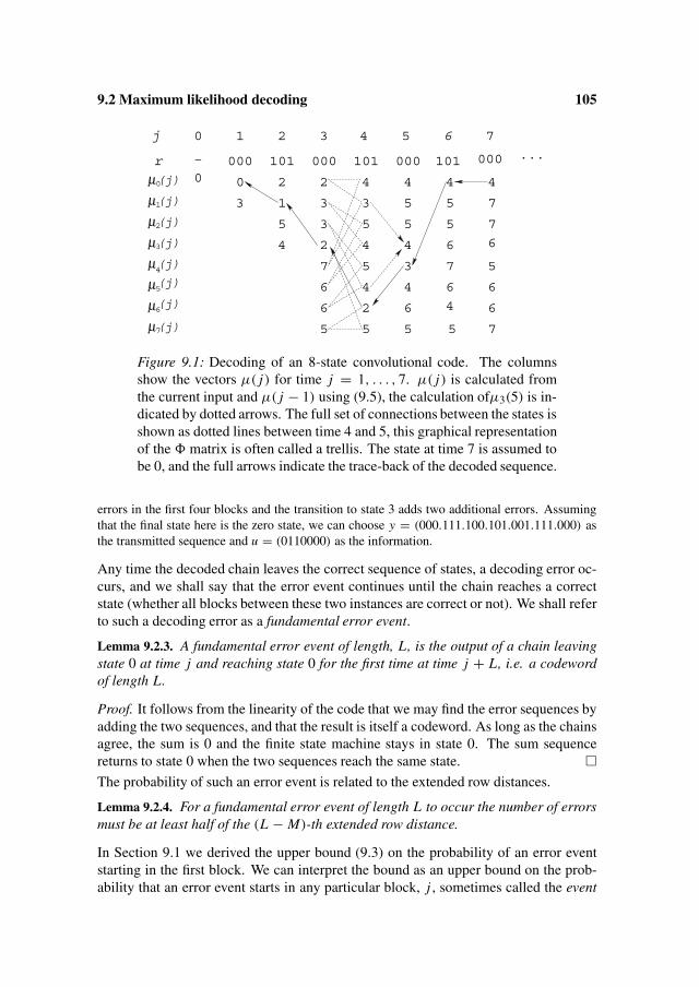
9.2 Maximum likelihood decoding 105
2
r 000 101 000 101 000 101 000 ...−
j 1 3 4 5 6 7
µµ
µµµµ
0
1
2
3
4
5
6
7(j)
(j)
(j)
(j)
(j)
µ(j)
(j)
(j)
0
0
2
6
5
6
4
5
7
6
6
0
3
2
1
5
4
2
3
3
7
6
6
5
4
3
5
4
5
4
2
5
5
5
4
3
4
5
4 4 4
5 7
6
57
6
7µ
Figure 9.1: Decoding of an 8-state convolutional code. The columnsshow the vectors µ( j) for time j = 1, . . . , 7. µ( j) is calculated fromthe current input and µ( j − 1) using (9.5), the calculation ofµ3(5) is in-dicated by dotted arrows. The full set of connections between the states isshown as dotted lines between time 4 and 5, this graphical representationof the matrix is often called a trellis. The state at time 7 is assumed tobe 0, and the full arrows indicate the trace-back of the decoded sequence.
errors in the first four blocks and the transition to state 3 adds two additional errors. Assumingthat the final state here is the zero state, we can choose y = (000.111.100.101.001.111.000) asthe transmitted sequence and u = (0110000) as the information.
Any time the decoded chain leaves the correct sequence of states, a decoding error oc-curs, and we shall say that the error event continues until the chain reaches a correctstate (whether all blocks between these two instances are correct or not). We shall referto such a decoding error as a fundamental error event.
Lemma 9.2.3. A fundamental error event of length, L, is the output of a chain leavingstate 0 at time j and reaching state 0 for the first time at time j + L, i.e. a codewordof length L.
Proof. It follows from the linearity of the code that we may find the error sequences byadding the two sequences, and that the result is itself a codeword. As long as the chainsagree, the sum is 0 and the finite state machine stays in state 0. The sum sequencereturns to state 0 when the two sequences reach the same state. �The probability of such an error event is related to the extended row distances.
Lemma 9.2.4. For a fundamental error event of length L to occur the number of errorsmust be at least half of the (L − M)-th extended row distance.
In Section 9.1 we derived the upper bound (9.3) on the probability of an error eventstarting in the first block. We can interpret the bound as an upper bound on the prob-ability that an error event starts in any particular block, j , sometimes called the event

106 Maximum likelihood decoding of convolutional codes
error probability. This probability is smaller than the probability of an error starting inthe first block because the decoder may select a wrong branch starting before time j .To arrive at the expected number of wrong blocks, the probabilities of the error eventsmust be multiplied by their length.
The Viterbi algorithm is a practical way of performing maximum likelihood decoding.The complexity is directly related to the number of states, and thus it increases expo-nentially with the memory of the code. Decoders with a few thousand states can beimplemented. It is an important aspect of the algorithm that it can use ‘soft decision’received values, i.e. real values of the noisy signal, rather than binary values. Theweights ei ′i , which we derived as the number of errors per block, may be replaced bythe logarithm of the conditional probability or a suitable approximation. Decoding forGaussian noise channels is discussed in Appendix A .
The algorithm can be used to perform ML decoding of block codes if they can be de-scribed as tail-biting codes. In principle other block codes can be decoded using thesame principle if the decoder is based on a finite state description of the encoder, butthe tail-biting structure is important as a way of keeping the number of states small.
9.3 Problems
Problem 9.3.1 Consider again the rate 12 convolutional code with generating vector
g = (11.10.01.11).
1) What are the codewords of weight 6?
2) How many states are there in the encoder?
3) If the input is a periodic repetition of 11100.11100. . . . , what is the encoded sequence?
4) Write out the transition matrix for the code.
5) Find the codewords of length 4, 5, and 6.
6) Find the weight enumerator of the code.
7) How many words of weight 7 and 8 are in the code?
8) Which of the following error patterns will always be correctly decoded?
a : 00.10.00.00.10.00 . . .
b : 01.10.00.00.00.00 . . .
c : 11.00.01.00.00.00 . . .
d : 11.00.00.00.00.11.00 . . .
e : 11.00.10.00.00.00 . . .
f : 00.00.00.01.11.00 . . .
9) Find an upper bound on the error probability using (9.3) when p = 0.01.
10) What is the largest value of p such that (9.3) gives a probability < 1?
11) Write out the E matrices needed for decoding.
12) Assume that there is a single error in the first block. Find those weights µ(i) that are less than4. Repeat the problem with two errors in the first block.
13) How can the information symbols be recovered from the decoded sequence?
9.3 Problems 107
Problem 9.3.2 Consider the (2, 1, 2) code in Example 8.1.1
1) In the transition matrix (z), replace z with variables x and y such that xi indicates i 0s andy j indicates j 1s. Calculate the two-variable weight enumerator.
2) How many codewords have four 0s and six 1s?
Problem 9.3.3 Consider the matrix in Example 8.1.1 with sequences (regular sets) as entries.
1) Find 2 and 3.
2) Check that the generator sequence appears in the expected place in the last matrix.
3) Set up the system of linear equations in regular sets as discussed in Section 9.1 and eliminateas many variables as possible by substitution.
4) In order to solve for ρ0 the following result is needed:
Let A, B, C be regular sets and A = B + AC; then A = BC∗.
Find a regular set description of the set of nonzero codewords.
5) Compare the results of 9.3.3 4) and 9.3.2 1).
Problem 9.3.4 (project) Use a program for symbolic computation to find the weight enumeratorof the convolutional code given in Problem 8.8.8.
Problem 9.3.5 (project)
1) Write a program for encoding and decoding the code from Problem 8.8.8.
2) Decode terminated frames of length 1000 information bits with bit error probability p = 0.02and p = 0.05.
3) Compare the results to the upper bounds.
4) Modify the encoder/decoder to use tail/biting frames.


Chapter 10
Combinations of several codes
As discussed in Chapter 7, long codes are often required to obtain sufficient reliabil-ity, but a single long block code or a convolutional code cannot provide the requiredperformance with an acceptable amount of computation. Here we give an introductionto coding methods where several codes, or several stages of coding, are combined in aframe. The difficulty of constructing good long codes led to this approach in an earlystage of the study of error-correcting codes, and it continues to be a focal point of muchdevelopment of communication systems.
If the length of the combined code is chosen to match the length of a transfer frame, theperformance is also directly related to the required frame error probability. We discussthe performance from this point of view, and also briefly mention some other issuesrelated to the application of such codes in communication systems or data storage.
When several codes are combined, the received symbols are stored in a buffer, and thedecoders work on only a subset of these symbols. In this way the total length will havean impact on the decoding delay and possibly other secondary properties of the sys-tem, but it does not directly determine the complexity of the decoding. The total codemay not have a very good minimum distance, but in most cases error patterns will bedecoded even though the weight exceeds half the minimum distance. Since the errorprobability depends on a combination of weights of error patterns and the number ofsuch patterns, a code with a relatively small number of low weight words can still havean acceptable performance.
10.1 Product codes
Product codes are the simplest form of composite codes, but nevertheless it is still aconstruction of interest.
Definition 10.1.1. A product code is a vector space of n1 by n2 arrays such that eachrow is a codeword in a linear (n1, k1, d1) code, and each column is a codeword in alinear (n2, k2, d2) code.

110 Combinations of several codes
Theorem 10.1.1. The parameters of a product code are (N,K ,D)=(n1n2,k1k2,d1d2).
Proof. The information symbols may be arranged in a k1 by k2 array. The paritychecks on rows and columns of information symbols may be computed independently.The parity checks on parity checks may be computed in two ways, but it follows fromlinearity that the results are the same: The last rows may be calculated as a linear com-bination of previous rows, and consequently they are codewords in the row code. Thus(N, K ) are the products stated in the lemma. The product of the minimum distances isa lower bound since a nonzero codeword has at least one nonzero row of weight at leastd1and each nonzero column has weight at least d2. A minimum distance codeword ofweight d1 may be repeated in d2 rows to form a codeword of weight exactly d1d2. Infact these are the only codewords of that weight. �For simplicity we shall assume that the row and column codes are identical with pa-rameters (n, k, d) unless different parameters are explicitly given.
In the simplest approach to decoding, each column of the received word is first decodedseparately, and a decoding algorithm for the row codes is then applied to the correctedword. We refer to such an approach as serial decoding.
Lemma 10.1.1. If a product code is decoded serially, any error pattern of weight atmost D−1
4 is decoded.
Proof. If d is odd, the worst case situation is that several columns contain d+12 errors
and are erroneously decoded. However given the total number of errors, there can be atmost d−1
2 such columns, and the errors will be decoded by the row codes. Of course, ifthe rows had been decoded first, the errors would have been decoded immediately. Onthe other hand an error pattern with at least d
2 errors in each row and column cannot be
decoded immediately, and thus we cannot be sure to decode⌈ d
2
⌉2errors. �
Any error pattern with at most D−12 errors can be corrected, but it is not trivial to extend
the decoding algorithm to reach this limit. Furthermore, to ensure small probability offrame error, the algorithm should also decode most errors of somewhat greater weight.We return to this decoding problem in Chapter 13.
The following lemma is useful for estimating the error probability.
Lemma 10.1.2. If the number of minimum weight codewords in the two componentcodes is a1 and a2, the number of words of weight d1d2 in the product code is a1a2.
Proof. Since the weight of a nonzero row is at least d1 and the weight of a columnis at least d2, a minimum weight codeword can have only d1 nonzero columns and d2nonzero rows. Thus the number of codewords of that weight is at most the number ofways of choosing the nonzero rows and columns such that there is a minimum weightcodeword on exactly those positions. On the other hand for any choice of a minimumweight row word and column word, there is a corresponding minimum weight word inthe product code. �

10.1 Product codes 111
For slightly higher weights the number of words can also be expressed in a fairly directway as indicated in the following example, however the relations become more com-plicated for higher weights. Thus we can get an upper bound on the error probabilityin the following form.
Theorem 10.1.2. For a product of binary (n, k, 2t) codes with weight distribution Aw ,the error probability is upper bounded by
P(e) ≤ 1
2A2
2t
(4t2
2t2
)p2t2 + · · ·
Proof. The result follows from Theorem 3.3.1. �Example 10.1.1. Product of extended Hamming codes
If the component codes are chosen as the extended Hamming code (64, 57, 4), the product codehas length N = 4096, rate K
N = 0.793, and minimum distance 16. If ML decoding is performed,the error probability can be estimated by the probability that eight errors occur within a set ofnonzero coordinates of a weight 16 word. The number of weight 4 codewords in the (64, 57)
code is
A4 =(64
3)
4= 10416
And the number of weight 16 words in the product code is the square of this number. FromTheorem 3.3.1 we get an upper bound on the error probability: Thus of the 12870 subsets of 16positions in a word, only 12 are shared with other minimum weight codewords. From Theorem10.1.2 we get an upper bound on the error probability:
P(e) ≤ 1
2·(
16
8
)· 104162 p8 + · · ·
Thus for p = 1/64 we get P(e) ≈ 0.0025. Of the 12870 subsets of 8 positions among the onesof a weight 16 word only 12 are shared with other minimum weight codewords. Thus this isa very close estimate for small p. The next term in the weight distribution of the product codeis A24, and it is possible to find the number of weight 24 codewords as the number of pairs ofweight 16 words that share four positions. It may then be verified that these words contributemuch less to the error probability. Thus a sufficiently powerful decoding algorithm could decodeon the average one error in each row and column, and if the frame is supplied with a frame checksequence, one could obtain adequate performance even for fairly large error probabilities.
Example 10.1.2. Product of RS codes
In composite coding systems Reed-Solomon codes play a particularly important role. The com-monly used codes are based on 8-bit symbols, q = 256. In some systems with very large frames(video), product codes of RS codes are used, and for complexity reasons the component codesare decoded only up to half the minimum distance. Improved performance may be achievedby reordering the symbols between the two codings. In common CDs, two stages of (short-ened) RS codes are used, and interleaving is used between the stages to spread out the effect ofconcentrated surface defects. Here both RS codes have distance only 4. The first stage of de-coding corrects single errors and detects double errors. After deinterleaving, the second decoderstage corrects the symbols that come from blocks with double errors. We refer to the technicalstandards for details of these systems.
112 Combinations of several codes
10.2 Concatenated codes (serial encoding)There are historical reasons for the use of the word ‘concatenate’, two encoders/de-coders were placed next to each other. The term does not quite reflect the way thecodes are combined. Some authors use the term serial to indicate that the output of thefirst stage of encoding is input into the second stage encoder. We shall use the termconcatenated code to indicate a combination of an RS (outer) code and a binary (inner)code, which is how the expression was originally used.
10.2.1 Parameters of concatenated codes
In Chapter 5 we defined a class of Reed-Solomon codes over the alphabet of q symbols(q a power of a prime) and parameters (N, K , D) = (q − 1, K , q − K ).
Lemma 10.2.1. The binary image of an RS code over the symbol field of q = 2r elementsis a binary (r(q − 1), r K , D′) code with D′ ≥ q − K .
Proof. The symbols in the big field are represented as binary r -vectors with additionrepresented as vector addition. We can find a basis for the binary image by convertinga row in the original generator matrix to r binary vectors. Let the original informationsymbol be a 1 in position j , 0 ≤ j < K , and consider the r − 1 codewords obtainedby multiplying this word by the first r − 1 powers of the primitive element used forconstructing the field. The images of these vectors have a 1 in one of the positionsjr to jr + r − 1. Since all elements in the big field are linear combinations of theser elements, we can get all images of the RS codewords as linear combinations of theKr binary vectors. The minimum weight of the binary image is at least the Hammingweight of the RS codeword. �The real minimum distance is difficult to analyze, and also of minor importance to thedecoding. However, we can get an upper bound using the construction of BCH codes(Chapter 6):
Lemma 10.2.2. The minimum distance of the binary image of an (N, K , D) RS code isupper bounded by the minimum distance of the BCH code CK (sub).
Proof. As discussed in Chapter 6, the BCH code is contained in the RS code. Takingthe binary image of a codeword that is already binary does not change its weight. Sincethe generator polynomial of the BCH code contains all roots in the generator polyno-mial of the RS code and some additional roots, its minimum distance may be greaterthan D. For RS codes of low rates, the bound is trivial, D ≤ N . �Now we combine the binary images of RS codes with a second binary coding stage ina way that is similar to the product codes. Let the information bits be represented as anr I by K array. Rows jr − r + 1 to jr are encoded as the binary image of an (N, K )
RS code, the j ’th outer code. Each column, which consists of a symbol from each RScode, is then encoded as a codeword from an (n, Ir, d) block code, the inner code. Theparameter I is referred to as the interleaving degree.

10.2 Concatenated codes (serial encoding) 113
Definition 10.2.1. A concatenated code with outer (q − 1, K ) RS code, interleaving de-gree I , and binary (n, I log q) inner code, is a binary (n(q − 1), K I log q) code, suchthat K log q information symbols are encoded as a binary image of the RS code, andfor each j , symbols j from each of the I RS codes are encoded as a codeword of theinner code.
Theorem 10.2.1. The minimum distance of the concatenated code is at least Dd.
Proof. In a nonzero word at least one RS code has D = q − K nonzero symbols. Theseare encoded by the inner code which has weight at least d in each nonzero column. �While a product code has many codewords with weight equal to the lower bound, a con-catenated code may have none or very few. If D′ is the minimum distance of CK (sub),there are codewords of weight D′d .
10.2.2 Performance of concatenated codes
The common decoding method for a concatenated code is to first decode the inner code.The information symbols obtained in this way are interpreted as symbols of the RScodewords, which are then decoded. As discussed in the case of product codes, serialcorrection of errors in the inner and outer code ensures only correction of Dd
4 errors. Ifmore than d
2 errors occur in a codeword of the inner code, a symbol error in the outercode may be produced, and only D−1
2 symbol errors can be corrected. However, witha random distribution of bit errors, most of them would be corrected by the inner code.
Let p be the bit error probability. For a given inner code and decoding method (whichwould usually be maximum likelihood decoding), the probability of decoding error forthe inner code, pi , can be found by one of the methods of Chapter 3.
The average number of symbol errors in a block of the RS code is µ = N pi . Sincethis is typically a small fraction of the block length and N is quite large, the Poissondistribution
P(t) = eµ µt
t !is a good approximation to the number of errors. We get a simple upper bound on thetail of the Poisson distribution by using a quotient series with quotient m
T +1 .
Lemma 10.2.3. If errors occur independently with probability, p, the probability thatthere are more than T errors in a block of N symbols is upper bounded by
�(p, T ) = e−N p(N p)T +1
(T + 1)!(
1 − N p(T +1)
)
Thus we have
Theorem 10.2.2. The probability of decoding failure for the concatenated code with anouter RS code correcting T errors and inner code decoding error probability, pi , isupper bounded by
Pf l < �(pi, T )

114 Combinations of several codes
Actual decoding errors are usually quite rare. The following theorem is a useful ap-proximation.
Theorem 10.2.3. The probability of decoding error for the concatenated code is approx-imately
Pue ≈ Pf l
T !Proof. Decoding of T = D−1
2 errors maps only a small fraction of the q N−K syn-
dromes on error patterns. Since there are about NT
T ! sets of error positions and qT setsof error values, the probability that a random syndrome corresponds to an error patternis 1
T ! . �For a typical RS code with T = 8 this factor is 40320 > 215. Thus in addition to cor-recting errors left by the inner code, the RS code provides a reduction of the probabilityof undetected error about equal to that of the 16 bit CRC check. It is consistent with thedefinitions in Chapter 7 to consider the check symbols of the RS code as the parity fieldin the data frame. However, since the outer code contributes to the error correction, theconvention in some contexts is to include it in the rate of the overall code, and in thisway it will also affect the information efficiency.
Example 10.2.1. A concatenated code
If we consider a moderately large field as F216 , we get (N, K ) RS codes which easily reach thelimits of practical frame sizes. However for shorter frames, interleaving of eight bit symbols isoften preferred. If two such codes are interleaved and each symbol is expressed in the usual wayas a binary vector of length 8, the total code is a linear binary (16N, 16K ) code. However, theminimum distance of the binary code may not be much larger than N − K . With (32, 16, 8)
inner codes we get codes of length 213. If the rate of the outer code is 34 , the total code has rate
38 and minimum distance 512 (the Varshamov-Gilbert bound for these parameters is D ≥ 1280).However, we get an acceptable performance even with an average number of errors per frame of460. With the bit error probability 460
8192 , Theorem 3.3.1 gives an upper bound on the decodingerror probability for the inner code of 0.055. Thus the RS code has to correct an average of14 errors, and a decoding failure caused by more than 32 errors has probability < 10−5. WithT = 32 the probability of undetected error is extremely small.
10.2.3 Interleaving and inner convolutional codes
The concatenated codes used in practice often have a convolutional code as the innercode. If the binary images of the I interleaved codes are written as an m I by N array,the array is encoded by the convolutional code one column at a time. The purpose ofthe interleaving, other than making the code longer, is to make the symbol errors ineach RS code almost independent. A precise analysis of such a code is difficult.
However, we can get a very similar code using a tail-biting version of the convolu-tional code as the inner code for each column. The advantage from the point of viewof the analysis is that the symbol errors in a particular outer code are mutually nowindependent.

10.2 Concatenated codes (serial encoding) 115
In tail-biting codes (and convolutional codes), there is a length associated with an er-ror event and a probability distribution on the lengths. What is relevant in this con-text is that the performance of the inner code may be characterized by probabilitiespi1, pi2, . . . , pi I that 1, 2, . . . , I consecutive outer code symbols in a particular col-umn are in error. Since a single long error event is more likely than two shorter events,we assume
pi j > pi1 pi, j−1
Clearly it may also occur that two non-consecutive symbols in the same column are inerror, but since this would be the result of two independent decoding errors, we maytreat this situation as errors in different columns. The probability that there is an errorin a column is
pc =∑
j
pi j
The average symbol error probability may be found as
ps = 1
I
∑j
j pi j
Clearly the probability of decoding failure is upper bounded by �(pc, T ), which fol-lows from using Theorem 10.2.1 with pc as the probability of error for the inner code.However, we can get a stronger bound.
Theorem 10.2.4. For a concatenated code with an inner convolutional code, where thesymbol error probability after decoding the inner code is Ps , the probability of frameloss is upper bounded as
Pfl < I�(ps, T )
Proof. For each RS code the probability of decoding failure is �(ps, T ). Thus for Iinterleaved codes the average number of RS codewords that are not decoded I timesthis number. The errors in different RS words within a frame are not independent, butthe theorem is true for any distribution of the words. �The actual performance is a little better since longer error events in the inner code tendsto cause more decoding failures in certain frames.
Even though several of the outer codewords cannot be decoded, there is often at leastone decoded RS word. Since this word has a very high probability of being correct,it would be possible to iterate the decoding of the inner and outer codes. In the posi-tions where errors have been corrected in the RS words, the decoding of the inner codeshould be repeated with the corrected symbols. However, it is difficult to analyze theimprovement in performance of such a procedure.
116 Combinations of several codes
10.3 ProblemsProblem 10.3.1 Consider a product of (7, 4, 3) Hamming codes.
1) What are the parameters of the code?
2) How many errors can be corrected if the rows and columns are decoded serially?
3) How many minimum weight words are there in the product code?
4) Describe a parity check matrix for the product code (without necessarily writing it out).
5) How can three errors be decoded if they are
a) in three different rows or columns?
b) in only two rows and columns?
Problem 10.3.2 Consider a product of (16, 12) RS codes over F16.
1) What are the parameters of the code?
2) How many errors can be corrected if we assume minimum distance decoding?
3) How many errors can be decoded if rows and columns are decoded serially?
Problem 10.3.3 Consider a product of the binary (5, 4) and (3, 2) even parity codes.
1) What are the parameters of the code?
2) Prove that the code is cyclic if the positions are taken in the proper order.
3) Find the generator polynomial of the cyclic code.
Problem 10.3.4 Consider the binary image of a (15, 10) RS code over F16.
1) What are the parameters of the code?
2) Change the code to a concatenated code with inner code (5, 4, 2). What are the parameters?
3) Change the code to interleaving degree 2 using the (9, 8, 2) code as inner code. What are theparameters?
Problem 10.3.5 Consider a (30, 20) RS code.
1) If the symbol error probability is 130 , what is the probability of decoding failure?
2) Under the same assumptions, what is the probability of decoding error?
3) The code is used as the outer code in a concatenated code with I = 2 and inner (14, 10, 3)code. If the bit error probability is 0.01, give an upper bound on the symbol error probability.
4) Give an upper bound on the probability of decoding failure for the concatenated code.
Problem 10.3.6 Let F16 be expressed as in Chapter 2, Example 2.2.3.
1) Find the coefficients of the generator polynomial for an RS code of length 15 correcting twoerrors.
2) Which binary code is contained in the RS code?
3) Let the generator matrix of a (7,4) Hamming code be as in Example 1.1.3. What are thecodewords representing the coefficients found in 1)?
10.3 Problems 117
4) Consider the concatenated code obtained by encoding the symbols of the RS code from ques-tion 1) using the code from 3). What are the parameters of the code? (You may use the resultof 2) to find the exact minimum distance).
5) Find a codeword in the concatenated code by taking the generator polynomial of the RS codeand encoding the symbols as in 4). Introduce seven bit errors in the nonzero symbols, anddecode the word.
Problem 10.3.7 (project) Use the interleaved RS code from Problem 10.3.5 and use the convo-lutional code from Problem 8.8.1 as the inner code. Compare decoding results for a single innercode and for a tail-biting code in each column.
Problem 10.3.8 (project) Write a decoding program for a (255, 239) RS code. Use this decoderfor a concatenated code with the (2, 1, 6) convolutional code from Problem 8.8.9 as inner code.Perform a simulation with 2% bit errors.


Chapter 11
Decoding Reed-Solomon and BCH-codes with the Euclidian algorithm
In this chapter we present the extended Euclidian algorithm for polynomials with coef-ficients in a (finite) field and then show how this can be used for the decoding of cycliccodes. Many practical decoders of Reed-Solomon codes use this method.
11.1 The Euclidian algorithmLet F be a field and let a(x), b(x) ∈ F[x] and suppose that deg(a(x)) ≥ deg(b(x)).
The Euclidian algorithm is used to determine a greatest common divisor, d(x), of a(x)
and b(x), and the extended version also produces two polynomials f (x) and g(x) suchthat
f (x)a(x) + g(x)b(x) = d(x)
The input to the algorithm is a(x) and b(x).
The algorithm operates with four sequences of polynomials ri (x), qi(x), fi (x) andgi (x).
The initialization is
r−1(x) = a(x), f−1(x) = 1, g−1(x) = 0
and
r0(x) = b(x), f0(x) = 0, g0(x) = 1
For i ≥ 1 the algorithm performs polynomial division of ri−2 by ri−1 to obtain thequotient qi and the new remainder ri (see section 2.2):
ri−2(x) = qi (x)ri−1(x) + ri (x), where deg(ri (x)) < deg(ri−1(x))
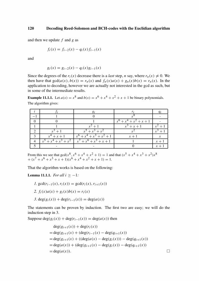
120 Decoding Reed-Solomon and BCH-codes with the Euclidian algorithm
and then we update f and g as
fi (x) = fi−2(x) − qi (x) fi−1(x)
and
gi (x) = gi−2(x) − qi(x)gi−1(x)
Since the degrees of the ri (x) decrease there is a last step, n say, where rn(x) �= 0. Wethen have that gcd(a(x), b(x)) = rn(x) and fn(x)a(x) + gn(x)b(x) = rn(x). In theapplication to decoding, however we are actually not interested in the gcd as such, butin some of the intermediate results.
Example 11.1.1. Let a(x) = x8 and b(x) = x6 + x4 + x2 + x + 1 be binary polynomials.
The algorithm gives:
i fi gi ri qi−1 1 0 x8 -0 0 1 x6 + x4 + x2 + x + 1 -1 1 x2 + 1 x3 + x + 1 x2 + 12 x3 + 1 x5 + x3 + x2 x2 x3 + 13 x4 + x + 1 x6 + x4 + x3 + x2 + 1 x + 1 x4 x5 + x4 + x3 + x2 x7 + x6 + x3 + x + 1 1 x + 15 - - 0 x + 1
From this we see that gcd(x8, x6 + x4 + x2 + 1) = 1 and that (x5 + x4 + x3 + x2)x8
+ (x7 + x6 + x3 + x + 1)(x6 + x4 + x2 + x + 1) = 1.
That the algorithm works is based on the following:
Lemma 11.1.1. For all i ≥ −1:
1. gcd(ri−1(x), ri (x)) = gcd(ri (x), ri+1(x))
2. fi (x)a(x) + gi (x)b(x) = ri (x)
3. deg(gi (x)) + deg(ri−1(x)) = deg(a(x))
The statements can be proven by induction. The first two are easy; we will do theinduction step in 3.
Suppose deg(gi(x)) + deg(ri−1(x)) = deg(a(x)) then
deg(gi+1(x)) + deg(ri (x))
= deg(gi+1(x) + (deg(ri−1(x) − deg(qi+1(x))
= deg(gi+1(x) + ((deg(a(x) − deg(gi(x))) − deg(qi+1(x))
= deg(a(x)) + (deg(gi+1(x) − deg(gi(x)) − deg(qi+1(x))
= deg(a(x)). �

11.2 Decoding Reed-Solomon and BCH codes 121
11.2 Decoding Reed-Solomon and BCH codes
Let C be a cyclic (n, k) code over Fq and suppose that the generator polynomial hasamong its zeroes the elements β, β2, . . . , β2t where β ∈ Fqm is an element of order n.
For the RS-codes we have n|q − 1 and t = ⌊ n−k2
⌋and for the binary BCH-codes we
have n|2m − 1 and dmin ≥ 2t + 1.
We know from Chapters 5 and 6 that if Q(x) = q0 + q1x + q2x2 + · · · + qt x t satisfies
S1 S2 . . . St+1S2 S3 . . . St+2...
... . . ....
St St+1 . . . S2t
q0q1q2...
qt
=
000...
0
(11.1)
where the syndromes Si are defined as Si = r(β i)
when r(x) is the received word,then the error locations (i.e. the powers of β that indicate the positions of the errors)are among the zeroes of Q(x).
If we define
S(x) =2t∑
i=1
Si x2t−i
and calculate S(x)Q(x), then (11.1) gives that the terms of degree t, t + 1, . . . , 2t − 1in S(x)Q(x) are all zero and therefore deg
(S(x)Q(x) mod x2t
)< t .
On the other hand if Q(x), with deg(Q(x)) ≤ t satifies that
deg(
S(X)Q(x) mod x2t)
< t
then we have a solution to (11.1)
Theorem 11.2.1. If the Euclidian algorithm is used on input a(x) = x2t and b(x) =S(x) and j is chosen s.t. deg(r j−1(x)) ≥ t and deg(r j (x)) < t , then Q(x) = g j (x).
Proof. It follows from Lemma 11.1.1 3 that deg(g j (x)) = 2t − deg(r j−1(x)) ≤ t . Bythe definition of j and from Lemma 11.1.1 2 we have that f j (x)x2t + g j (x)S(x) =r j (x). Since deg(r j (x)) < t we then get that deg
(g j (x)S(x) mod x2t
)< t and there-
fore the theorem is proved. �
Example 11.2.1. A (15, 5, 7) binary code
Let α be a primitive element of F16 where α4 +α+1 = 0. Let C be the cyclic code with genera-tor polynomial g(x) = mα(x)mα3(x)mα5 (x) = (x4+x+1)(x4 +x3+x2 +x+1)(x2 +x+1) =x10 + x8 + x5 + x4 + x2 + x + 1.
So C is a (15, 5, 7) code.

122 Decoding Reed-Solomon and BCH-codes with the Euclidian algorithm
Let the received word be r(x) = x4 + x2 + x + 1. The syndromes are
S1 = r(α) = 1 + α2 + α5 + α6 = 1
S2 = S12 = 1
S3 = r(α3) = 1 + α6 + α15 + α3 = α7
S4 = S22 = 1
S5 = r(α5) = 1 + α10 + α10 + 1 = 0
S6 = S32 = α14
We therefore have S(x) = x5 + x4 + α7x3 + x2 + α14.
The Euclidian algorithm on x6 and S(x) gives:
i gi ri qi−1 0 x6 -0 1 x5 + x4 + α7x3 + x2 + α14 -1 x + 1 α13x4 + α13x3 + x2 + α14x + α14 x + 12 α2x2 + α2x + 1 α12x3 + α12x2 + αx + α14 α2x3 α3x3 + α3x2 + α12x + 1 α9x2 + α11x + α14 αx
From this we see that j = 3 and g3(x) = α3x3 + α3x2 + α12x + 1, which has α8, α9 and α10
as zeroes, so the error vector is x10 + x9 + x8 and the codeword is therefore x10 + x9 + x8 +x6 + x5 + x2 + 1 ( = g(x)).
Example 11.2.2. A (15, 9, 7) Reed-Solomon code over F16
Let α be a primitive element of F16 where α4 + α + 1 = 0 and let C be the (15, 9, 7)
Reed-Solomon code over F16 obtained by evaluation of polynomials of degree at most 8 inα0, α, . . . , α14. Then C has generator polynomial g(x) = (x − α)(x − α2)(x − α3)(x − α4)
(x − α5)(x − α6) = x6 + α10x5 + α14x4 + α4x3 + α6x2 + α9x + α6.
Let r(x) = x8 + α14x6 + α4x5 + α9x3 + α6x2 + α be a received word.
The syndromes are
S1 = r(α) = α8 + α5 + α9 + α12 + α8 + α = 1
S2 = r(α2) = α + α11 + α14 + 1 + α10 + α = 1
S3 = r(α3) = α9 + α2 + α4 + α2 + α = α3
S4 = r(α)4 = α2 + α8 + α9 + α6 + α14 + α = α
S5 = r(α5) = α10 + α14 + α14 + α9 + α + α = α13
S6 = r(α6) = α3 + α5 + α4 + α12 + α3 + α = α3
We therefore have S(x) = x5 + x4 + α3x3 + α6x2 + α13x + α3.

11.2 Decoding Reed-Solomon and BCH codes 123
The Euclidian algorithm on x6 and S(x) gives:
i gi ri qi−1 0 x6 -0 1 x5 + x4 + α3x3 + α6x2 + α13x + α3 -1 x + 1 α14x4 + α5x3 + x2 + α8x + α3 x + 12 α2x2 + α4x α11x3 + α10x2 + +α7x αx + 13 α4x3 + α3x2 + α9x + 1 α7x2 + αx + α3 α3x + α3
The polynomial g3(x) has as zeroes 1, α4 and α7, so the error polynomial is e(x) = e1 +e2x4 +e3x7.
To find the error values one can solve the system of equations:
S1 = 1 = e(α) = e1 + e2α4 + e3α7 (11.2)
S2 = 1 = e(α2) = e1 + e2α8 + e3α14 (11.3)
S3 = α3 = e(α3) = e1 + e2α12 + e3α6 (11.4)
The solution is e1 = α, e2 = α6 and e3 = α10 so we get e(x) = α10x7 +α6x4 +α and thereforec(x) = r(x) + e(x) = x8 + α10x7 + α14x6 + α4x5 + α6x4 + α9x3 + α6x2(= x2g(x)).
The error values can be found directly using a formula (due to D. Forney) that we willnow derive. Before doing that we will introduce a useful concept.
Definition 11.2.1. Let a(x) = anxn + · · · + a1x + a0 be a polynomial in Fq [x].Then a′(x) = nan xn−1 + · · · + 2a2x + a1 where the integers i in the coefficients arethe sum of i 1s in the field.
With this definition it is easy to see that
(a(x) + b(x))′ = a′(x) + b′(x) and (a(x)b(x))′ = a′(x)b(x) + a(x)b′(x).
Let the error positions be xi1 , xi2 , . . . , xit with the corresponding error values ei1 , ei2 ,. . . , eit . Using the notation from Theorem 11.2.1 we will prove
Theorem 11.2.2.
eiS = −x−(2t+1)iS
r j(xiS
)
g′j
(xiS
) (11.5)
Proof. From (5.6) we have that
eiS =∑t
r=1 P(S)r Sr
P(S)(xiS )
where
P(S)(x) =t∑
r=1
P(S)r xr = (−1)S−1x
t∏l=1l �=S
(x − xil
)and Sr =
t∑j=1
ei j xri j.
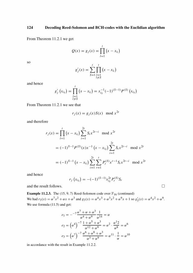
124 Decoding Reed-Solomon and BCH-codes with the Euclidian algorithm
From Theorem 11.2.1 we get
Q(x) = g j (x) =t∏
l=1
(x − xil
)
so
g′j (x) =
t∑S=1
t∏l=1l �=S
(x − xil
)
and hence
g′j
(xiS
) =t∏
l=1l �=S
(x − xil
) = x−1iS
(−1)(S−1)P(S)(xiS
)
From Theorem 11.2.1 we see that
r j (x) = g j (x)S(x) mod x2t
and therefore
r j (x) =t∏
l=1
(x − xil
) 2t∑i=1
Si x2t−i mod x2t
= (−1)S−1P(S)(x)x−1 (x − xiS
) 2t∑i=1
Si x2t−i mod x2t
= (−1)S−1 (x − xil
) 2t∑i=1
t∑r=1
P(S)r xr−1Si x2t−i mod x2t
and hencer j(xiS
) = −(−1)(S−1)x2tiS
P(S)r Sr
and the result follows. �Example 11.2.3. The (15, 9, 7) Reed-Solomon code over F16 (continued)
We had r3(x) = α7x2 + αx + α3 and g3(x) = α4x3 + α3x2 + α9x + 1 so g′3(x) = α4x2 + α9.
We use formula (11.5) and get:
e1 = −−7 α7 + α + α3
α4 + α9
1
α14= α
e2 =(α4)−7 1 + α5 + α3
α12 + α9= α2 · α12
α8= α6
e3 =(α7)−7 α6 + α8 + α3
α3 + α9= α11 · 1
α= α10
in accordance with the result in Example 11.2.2.
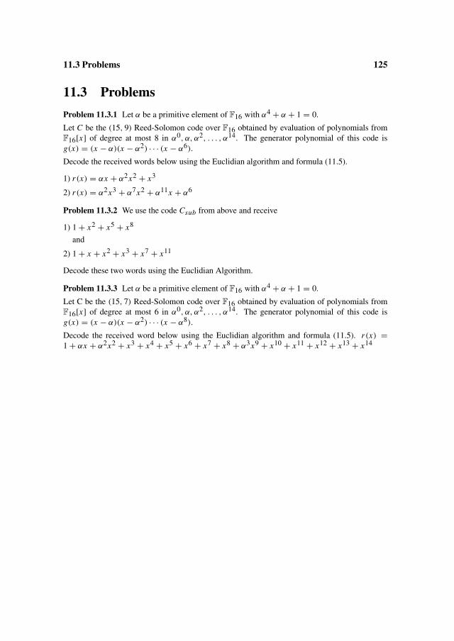
11.3 Problems 125
11.3 Problems
Problem 11.3.1 Let α be a primitive element of F16 with α4 + α + 1 = 0.
Let C be the (15, 9) Reed-Solomon code over F16 obtained by evaluation of polynomials fromF16[x] of degree at most 8 in α0, α, α2, . . . , α14. The generator polynomial of this code isg(x) = (x − α)(x − α2) · · · (x − α6).
Decode the received words below using the Euclidian algorithm and formula (11.5).
1) r(x) = αx + α2x2 + x3
2) r(x) = α2x3 + α7x2 + α11x + α6
Problem 11.3.2 We use the code Csub from above and receive
1) 1 + x2 + x5 + x8
and
2) 1 + x + x2 + x3 + x7 + x11
Decode these two words using the Euclidian Algorithm.
Problem 11.3.3 Let α be a primitive element of F16 with α4 + α + 1 = 0.
Let C be the (15, 7) Reed-Solomon code over F16 obtained by evaluation of polynomials fromF16[x] of degree at most 6 in α0, α, α2, . . . , α14. The generator polynomial of this code isg(x) = (x − α)(x − α2) · · · (x − α8).
Decode the received word below using the Euclidian algorithm and formula (11.5). r(x) =1 + αx + α2x2 + x3 + x4 + x5 + x6 + x7 + x8 + α3x9 + x10 + x11 + x12 + x13 + x14


Chapter 12
List decoding of Reed-Solomon codes
In this chapter we will extend the decoding method presented in Chapter 5 for Reed-Solomon codes in a way that allows correction of errors of weight greater than half theminimum distance. In this case the decoder gives a list of closest codewords, so themethod is called list decoding.
12.1 A list decoding algorithmRecall that if X = {x1, x2, . . . , xn} ⊆ Fq and k ≤ n, then the Reed-Solomon codeconsists of all the words of the form
( f (x1), f (x2), . . . , f (xn))
where f (x) ∈ Fq [x] has degree < k. The parameters are (n, k, n − k + 1).
Let r ∈ nFq be a received word, and suppose r is the sum of a codeword c and an error
vector e of weight at most τ . The idea here is an extension of the method presented inChapter 5, namely to determine a bivariate polynomial
Q(x, y) = Q0(x) + Q1(x)y + Q2(x)y2 + · · · + Ql (x)yl
such that:
1. Q(xi , ri ) = 0, i = 1, 2, . . . , n.
2. deg(Q j (x)) ≤ n − τ − 1 − j (k − 1), j = 0, 1, . . . , l.
3. Q(x, y) �= 0.
We then have
Lemma 12.1.1. If Q(x, y) satisfies the above conditions and c = ( f (x1), f (x2), . . . ,f (xn)) with deg( f (x)) < k, then (y − f (x))|Q(x, y).

128 List decoding of Reed-Solomon codes
Proof. The polynomial Q(x, f (x)) has degree at most n − τ − 1 but since ri = f (xi )
except in at most τ cases we have that Q(xi , f (xi )) = 0 in at least n − τ cases andtherefore Q(x, f (x)) = 0. If we consider the polynomial Q(x, y) as a polynomial iny over Fq [x], we then conclude that (y − f (x)) divides Q(x, y). �This means that we can find all the codewords that are within distance at most τ fromthe received word by finding factors of the polynomial Q(x, y) of the form (y − f (x))
with deg( f (x)) < k. If τ is greater than half the minimum distance it is possible thatwe get more than one codeword (a list), but since the y-degree of Q(x, y) is at most l,there are at most l codewords on the list. Not all factors may correspond to a codewordwithin distance τ to the received word.
It is not obvious under which conditions, on the numbers τ and l, a polynomial Q(x, y)
that satisfies the conditions actually exists, but the following analysis adresses thisquestion.
The first condition is a homogeneous system of n linear equations so if the number ofunknowns is greater than n this system indeed has a nonzero solution. The number ofunknowns is (n −τ )+ (n −τ − (k −1))+ (n −τ −2(k −1))+· · ·+ (n −τ − l(k −1)).This number equals (l + 1)(n − τ ) − 1
2 l(l + 1)(k − 1), so the condition becomes
(l + 1)(n − τ ) − 1
2l(l + 1)(k − 1) > n (12.1)
or equivalently
τ < nl
l + 1− l
2(k − 1) (12.2)
and in order that condition (12.2) gives a nonnegative degree we must also have that
(n − τ ) − l(k − 1) ≥ 0 (12.3)
or equivalentlyτ ≤ n − l(k − 1) (12.4)
If l = 1 condition (12.2) becomes τ < n−k+12 which is half the minimum distance.
If l = 2 we get τ < n − 2(k − 1) if kn ≥ 2
3 + 1n and this is smaller than half the
minimum distance! If kn < 2
3 + 1n then we get τ < 2
3 n − (k − 1) and this is smallerthan half the minimum distance if k
n ≥ 13 + 1
n . So we only get an improvement on halfthe minimum distance if k
n < 13 + 1
n .
This illustrates the general situation: In order to get an improvement on half the mini-mum distance the parameters should satisfy
k
n<
1
l + 1+ 1
n
and in this case
τ < nl
l + 1− l
2(k − 1)

12.1 A list decoding algorithm 129
Example 12.1.1. List of 2 decoding of a (15, 3) Reed- Solomon code over F16.
Let α be a primitive element of F16 where α4 + α3 + 1 = 0 and consider the (15, 3) Reed-Solomon code obtained by evaluating polynomials of degree at most 2 in the powers of α. Thecode has minimum distance 13 and is thus 6-error correcting. However using the above withl = 2 we see that it is possible to decode up to seven errors with list size at most 2.
If w = (0, 0, 0, 0, 0, 0, 0, 0, α6, α2, α5, α14, α, α7, α11)
is received one finds
Q(x, y) = (1+ x)y + y2 = (y −0)(y − (1+ x)) and the corresponding two codewords are then
(0, 0, 0, 0, 0, 0, 0, 0, 0, 0, 0, 0, 0, 0, 0) and
(0, α12, α9, α4, α3, α10, α8, α13, α6, α2, α5, α14, α, α7, α11)
The list of l decoding algorithm can be presented as follows.
Algorithm 12.1.1. List decoding of RS codes (Sudan)
Input: A received word r = (r1, r2, . . . , rn), and a natural number τ
1. Solve the system of linear equations
l∑j=0
r1j . . . 0 0
0 r2j . . . 0
......
. . . 00 0 . . . rn
j
1 x1 . . . xl j1
1 x2 . . . xl j2
...... . . .
...
1 xn . . . xl jn
Q j,0Q j,1Q j,2
...
Q j,l j
=
000...
0
Here l j = n − τ − 1 − j (k − 1).
2. Put
Q j (x) =l j∑
r=0
Q j,r xr
and
Q(x, y) =l∑
j=o
Q j (x)y j .
3. Find all factors of Q(x, y) of the form (y − f (x)) with deg ( f (x)) < k.
Output: A list of the factors f (x) that satisfyd ( f (x1), f (x2), . . . , f (xn), (r1, r2, . . . , rn)) ≤ τ
We will return to the factorization problem in Section 12.3. It follows from the aboveanalysis that if τ < n l
l+1 − l2 (k − 1), then the sent codeword is on the resulting list.

130 List decoding of Reed-Solomon codes
12.2 An extended list decoding algorithmAs we have seen the method described in the previous section only works for low ratesof the codes. In this section we discuss an improvement that works for all rates. Inorder to explain this, we first define what we mean by the multiplicity of a zero of abivariate polynomial.
Definition 12.2.1. Let Q(x, y) = ∑qi, j x i y j be a polynomial in Fq [x, y].
Let (a, b) ∈ nFq2 and let Q∗(x, y) = Q(x + a, y + b) = ∑
q∗i, j x i y j .
If q∗i, j = 0 for i + j < s and s is the largest such number, then (a, b) is said to be a
zero of Q(x, y) of multiplicity s.
The polynomial Q(x, y) = 1 + x2 + y2 + x2y2 ∈ F2[x, y] has (1, 1) as a zero ofmultiplicity 4 since Q(x + 1, y + 1) = x2y2.
We note that if Q(x, y) has (a, b) as a zero of multiplicity s, this corresponds to(s+1
2
)homogeneous linear equations in the coefficients.
Let C be a Reed-Solomon code and let r be a received word, that is the sum of acodeword c and an error vector of weight at most τ . We then determine a bivariatepolynomial
Q(x, y) = Q0(x) + Q1(x)y + Q2(x)y2 + · · · + Ql (x)yl
such that:
1. (xi , ri ), i <= 1, 2, . . . , n are zeroes of Q(x, y) of multiplicity s.
2. deg(Q j (x)) ≤ s(n − τ ) − 1 − j (k − 1), j = 0, 1, . . . , l.
3. Q(x, y) �= 0.
We then have
Lemma 12.2.1. If Q(x, y) satisfies the above conditions and c = ( f (x1), . . . , f (xn))
with deg( f (x)) < k, then (y − f (x))|Q(x, y).
Proof. We first prove that if f (xi) = ri , then (x − xi )s |Q(x, f (x)). To see this let
p(x) = f (x + xi ) − ri ; we then have p(0) = 0 and therefore x |p(x).If h(x) = Q(x + xi , p(x) + wi ) it follows from condition 1 that h(x) has no terms ofdegree smaller than s so xs |h(x) and therefore (x − xi )
s |h(x − xi ). Since h(x − xi) =Q(x, f (x)) the claim is proved.
Now the proof of the lemma follows by noting that the polynomial Q(x, f (x)) hasdegree at most s(n − τ ) − 1. But (x − xi )
s |Q(x, f (x)) for at least n − τ x ′i s and
therefore Q(x, f (x)) is divisible by a polynomial of degree at least s(n − τ ) and henceQ(x, f (x)) = 0. �

12.2 An extended list decoding algorithm 131
This implies that we can find all the codewords of distance at most τ from the receivedword by finding factors of Q(x, y) of the form (y − f (x)) with deg( f (x)) < k.
In order to ensure the existence of a polynomial Q(x, y) that satisfies the three condi-tions, we first note that condition 2 only gives nonnegative degrees if
s(n − τ ) − l(k − 1) ≥ 0 (12.5)
or equivalently
τ ≤ n − l(k − 1)
s(12.6)
The first condition is a system of n(s+1
2
)homogeneous linear equations, so if the num-
ber of unknowns is greater than this number the system has a nonzero solution. Thecondition is
(l + 1)s(n − τ ) − 1
2l(l + 1)(k − 1) > n
(s + 1
2
)(12.7)
or equivalently
τ <n(2l − s + 1)
2(l + 1)− l(k − 1)
2s(12.8)
A detailed analysis of the numbers involved shows that if s < l, then we get an im-provement on half the minimum distance if
k
n≤ 1
n+ s
l + 1(12.9)
Example 12.2.1. List of 4 decoding of a (63, 31) Reed-Solomon code over F64.
The code has minimum distance 33, but with s = 3 and l = 4 we can correct 17 errors.
We can now formulate the algorithm.
Algorithm 12.2.1. List decoding of RS codes (Gurusami-Sudan)
Input: A received word (r1, r2, . . . , rn) and natural numbers τ and s
1. Solve for Qa,b the system of linear equations, h + r < s and i = 1, 2, . . . , n.
∑a≥hb≥r
(a
h
)(b
r
)Qa,bxa−h
i rb−ri = 0 (12.10)
with Qa, b = 0 if l > a or b > la where la = s(n − τ ) − 1 − a(k − 1).
2. Put
Q j (x) =l j∑
r=0
Q j,r xr and Q(x, y) =l∑
j=0
Q j (x)y j
3. Find all factors of Q(x, y) of the form (y − f (x)) with deg ( f (x)) < k
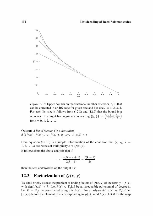
132 List decoding of Reed-Solomon codes
0 0.1 0.2 0.3 0.4 0.5 0.6 0.7 0.8 0.9 10
0.1
0.2
0.3
0.4
0.5
0.6
0.7
0.8
k/n
τ/n
Figure 12.1: Upper bounds on the fractional number of errors, τ/n, thatcan be corrected in an RS code for given rate and list size l = 1, 2, 3, 4.For each list size it follows from (12.8) and (12.9) that the bound is a
sequence of straight line segments connecting( k
n , τn
) =(
s(s+1)l(l+1)
, l−sl+1
)
for s = 0, 1, 2, . . . , l.
Output: A list of factors f (x) that satisfyd (( f (x1), f (x2), . . . , f (xn)) , (r1, r2, . . . , rn)) < τ
Here equation (12.10) is a simple reformulation of the condition that (xi , ri ), i =1, 2, . . . , n are zeroes of multiplicity s of Q(x, y).
It follows from the above analysis that if
τ <n(2l − s + 1)
2(l + 1)− l(k − 1)
2s
then the sent codeword is on the output list.
12.3 Factorization of Q(x, y)
We shall briefly discuss the problem of finding factors of Q(x, y) of the form y − f (x)
with deg( f (x)) < k. Let h(x) ∈ Fq [x] be an irreducible polynomial of degree k.Let E = Fqk be constructed using this h(x). For a polynomial p(x) ∈ Fq [x] let[p(x)] denote the element in E corresponding to p(x) mod h(x). Let be the map

12.3 Factorization of Q(x, y) 133
: Fq [x, y] → E[y] given by
(∑i
pi (x)yi
)=∑
i
[pi(x)]yi (12.11)
So the effect of the mapping is to reduce all the pi (x) modulo h(x) and therefore (Q(x, y)) can be considered as an element of Fqk [y]. It is not hard to see that
(Q1 Q2) = (Q1) (Q2) and (Q1 + Q2) = (Q1) + (Q2)
based on this observation one can prove
Lemma 12.3.1. If (y − f (x))|Q(x, y), then y − [ f ] is a factor of (Q(x, y)).
This means that the factorization problem is reduced to factoring univariate polynomi-als over Fqk and there are efficient algorithms (in most symbolic computing languages)for doing this. Actually some of these packages can factor Q(x, y) directly.
Example 12.3.1. We consider the (15, 7, 9) Reed-Solomon code over F16 where α is a primitiveelement of F16 satisfying α4 + α + 1 = 0 and xi = αi−1, i = 1, 2, . . . , 15.
With s = 4 and l = 6 we can list decode five errors.
Let the received word be r = (0, 0, α11, 0, α12, α11, 0, 0, 0, 0, 0, 0, α3, 0, α7).
If we use the method of Section 12.2 we get
Q(x, y) = (α5 + α4x + α2x2 + x3 + α7x4 + α3x5 + α6x6 + α3x7 + α7x8 + α6x9
+ α10x10 + α13x11 + α9x12 + α10x13 + α3x14 + α11x15 + x17 + α14x18
+ α2x19 + α4x20 + α10x21 + α12x22 + α6x24 + α2x25 + α2x26 + αx27
+ α3x28 + α8x29 + α9x31 + α13x32 + x33)y
+ (α4x + x2 + α11x3 + α8x4 + x5 + α14x6 + α3x7 + α14x8 + α5x9
+ α7x10 + α11x11 + α6x12 + αx13 + α9x14 + α11x15 + αx16
+ α13x17 + α11x18 + α11x19 + α14x20 + α10x21 + α5x22
+ α13x23 + αx24 + α4x25 + α3x26 + α9x27)y2
+ (α9 + α5x + α9x2 + α3x3 + α10x4 + α4x6 + α9x15 + α5x16
+ α9x17 + α3x18 + α10x19 + α4x21)y3
+ (α2 + α3x + α5x2 + α10x3 + αx4 + α10x5 + α14x7 + α4x8 + α5x9 + α12x10
+ α12x11 + α12x12 + x13 + x14)y4
+ (α12 + α14x+α13x2 + α4x3 + α10x4 + α9x5 + α11 + x6 + α4x7 + α8x8)y5
+ (αx + α8x2)y6

134 List decoding of Reed-Solomon codes
The polynomial h(x) = 1+α11x +α6x2 +α8x3 +α11x4 +α12x5 +α13x6 + x7 is irreducibleover F16 and using that we get
(Q(x, y)) = (α8 + α14x + α9x2 + α10x3 + x4 + α5x5 + α12x6)y
+ (α8 + αx + α11x2 + α4x3 + α7x4 + α6x5 + α6x5 + x6)y2
+ (α8 + α10x + α8x2 + x3 + α2x4 + x5)y3
+ (α4 + α14x + α8x2 + α11x3 + α9x4 + α9x5 + αx6)y4
+ (α5 + α2x + x2 + α9x3 + αx4 + α3x5 + x6)y5
+ y6
The factorization of this polynomial into irreducible factors over F167 gives
(Q(x, y)) = y((α4 + α10x + α11x2 + α9x3 + α4x4 + α9x5 + x6) + y
)((1 + α14x + α3x2 + α5x3 + α7x4 + α3x5 + αx6)
+ (α13 + α10x + α7x2 + αx3 + α10x4 + α7x5 + α4x6)y
+ (α8 + α8x + α12x2 + α3x3 + α13x4 + α6x6)y2
+(α8 + α4x + α12x2 + x4 + αx5)y3 + y4)
The factor (α4 + α10x + α11x2 + α9x3 + α4x4 + α9x5 + x6) + y corresponds to a word withdistance 14 from the received word r and the only other degree 1 factor is y, so in this case weonly get one word on the list, namely the all 0s word and therefore the decoding was not onlycorrect but also unique. Actually this is the typical case.
If we consider the same situation as above and receive
r = (1, 0, 0, 1, 0, 0, 1, 0, 0, 1, 0, 0, 1, 0, 0)
we getQ(x, y) = (α14 + α14x10 + α14x20)y2 + (α14 + α14x10)y4 + α14y6
and
(Q(x, y)) = (α11 + α6x2 + α2x3 + α10x4 + α8x5 + α2x6)y2
+ (α8 + α6x + α5x2 + α8x4 + α10x5 + x6)y4 + y6
The factorization gives:
(Q(x, y)) =((α5 + α10x5) + y
)2 ((α10 + α5x5) + y
)2y2
This in turn corresponds to three codewords, all with distance 5 to r , namely
(0, 0, 0, 0, 0, 0, 0, 0, 0, 0, 0, 0, 0, 0, 0)
(1, α10, 0, 1, α10, 0, 1, α10, 0, 1, α10, 0, 1, α10, 0)
and(1, 0, α5, 1, 0, α5, 1, 0, α5, 1, 0, α5, 1, 0, α5)
12.4 Problems 135
12.4 ProblemsProblem 12.4.1
1) How many errors can be corrected with a list size 2 in a (31,10) Reed-Solomon code over F32?
2) With list size 3?
Problem 12.4.2 A (31, 5) Reed-Solomon code over F32 is list decoded. What list size shouldbe used in order to correct as many errors as possible?
Problem 12.4.3 Consider the (10,3,8) Reed-Solomon code over F11 with xi = 2i−1, i =1, 2, . . . , 10
1) How many errors can be corrected with list size 2?
2) If (0, 0, 6, 9, 1, 6, 0, 0, 0, 0) is received and we decode with list size 2, show that Q(x, y) =y2 − y(x2 − 3x + 2).
3) What are the possible sent codewords?
Problem 12.4.4 Consider a (31,15) Reed-Solomon code over F32. If this is list decoded usingthe extended algorithm, how many errors can be corrected using different values of l and s?

Chapter 13
Iterative decoding
In Chapter 10 we discussed several ways of building a frame structure from smallercomponent codes. Here we discuss decoding of composite codes based on iterating thedecoding of the components. Our starting point is a type of long codes where the partsare rather loosely connected, and in this way some decoding decisions can be madebased on local information. In the development of coding theory this was one of theearly approaches, although it has only recently become a subject of wide interest.
13.1 Low density parity check codesAs discussed in Chapter 1, a block code is defined by its parity check matrix, H , andevery row in H indicates a parity check that all words satisfy. A code has many equiv-alent parity check matrices, but for codes under consideration here we concentrate ona particular matrix with a useful property. Sometimes it is useful to specify a matrixwith more than N − k rows to get a desirable structure. Thus in this chapter we shallnot require that the rows of H are linearly independent.
Definition 13.1.1. A low-density parity check (LDPC) code with parameters (N, i, j)has block length N and a parity check matrix with j 1s in each row and i 1s in eachcolumn. N is usually much larger than i and j .
Lemma 13.1.1. The rate of an (N, i, j) LDPC satisfies
R ≥ 1 − i
j
Proof. If H has b rows, the total number of 1s is bj = Ni . These rows may not all belinearly independent, and thus the dimension k of the code satisfies
k ≥ N − b = N − Ni
j
Let the parity check matrix be indexed as H = [huv]. It is convenient to refer to theset of row indices in column v such that huv = 1 as Iv , and Ju is similarly the set of
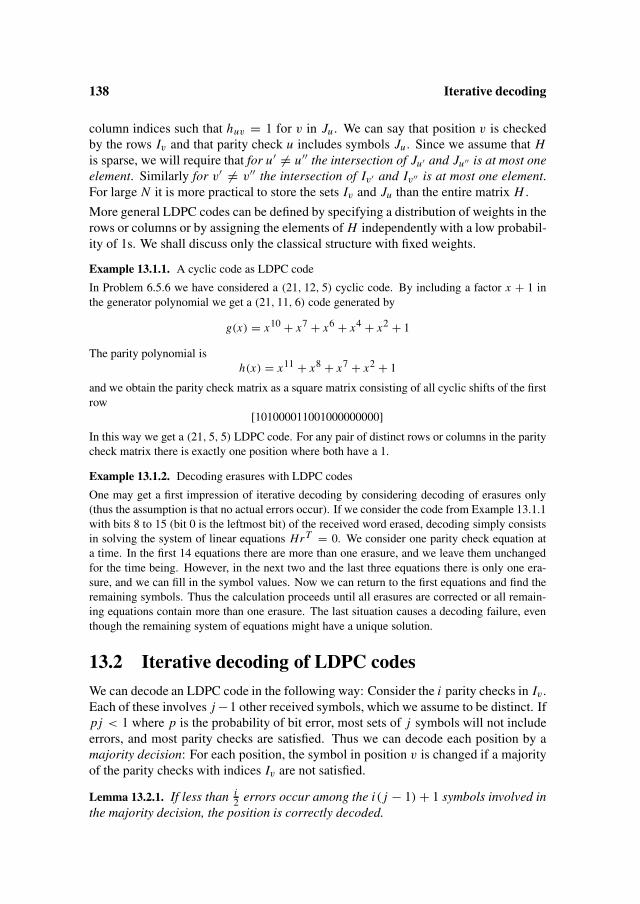
138 Iterative decoding
column indices such that huv = 1 for v in Ju . We can say that position v is checkedby the rows Iv and that parity check u includes symbols Ju . Since we assume that His sparse, we will require that for u′ �= u′′ the intersection of Ju′ and Ju′′ is at most oneelement. Similarly for v′ �= v′′ the intersection of Iv′ and Iv′′ is at most one element.For large N it is more practical to store the sets Iv and Ju than the entire matrix H .
More general LDPC codes can be defined by specifying a distribution of weights in therows or columns or by assigning the elements of H independently with a low probabil-ity of 1s. We shall discuss only the classical structure with fixed weights.
Example 13.1.1. A cyclic code as LDPC code
In Problem 6.5.6 we have considered a (21, 12, 5) cyclic code. By including a factor x + 1 inthe generator polynomial we get a (21, 11, 6) code generated by
g(x) = x10 + x7 + x6 + x4 + x2 + 1
The parity polynomial ish(x) = x11 + x8 + x7 + x2 + 1
and we obtain the parity check matrix as a square matrix consisting of all cyclic shifts of the firstrow
[101000011001000000000]In this way we get a (21, 5, 5) LDPC code. For any pair of distinct rows or columns in the paritycheck matrix there is exactly one position where both have a 1.
Example 13.1.2. Decoding erasures with LDPC codes
One may get a first impression of iterative decoding by considering decoding of erasures only(thus the assumption is that no actual errors occur). If we consider the code from Example 13.1.1with bits 8 to 15 (bit 0 is the leftmost bit) of the received word erased, decoding simply consistsin solving the system of linear equations Hr T = 0. We consider one parity check equation ata time. In the first 14 equations there are more than one erasure, and we leave them unchangedfor the time being. However, in the next two and the last three equations there is only one era-sure, and we can fill in the symbol values. Now we can return to the first equations and find theremaining symbols. Thus the calculation proceeds until all erasures are corrected or all remain-ing equations contain more than one erasure. The last situation causes a decoding failure, eventhough the remaining system of equations might have a unique solution.
13.2 Iterative decoding of LDPC codesWe can decode an LDPC code in the following way: Consider the i parity checks in Iv .Each of these involves j −1 other received symbols, which we assume to be distinct. Ifpj < 1 where p is the probability of bit error, most sets of j symbols will not includeerrors, and most parity checks are satisfied. Thus we can decode each position by amajority decision: For each position, the symbol in position v is changed if a majorityof the parity checks with indices Iv are not satisfied.
Lemma 13.2.1. If less than i2 errors occur among the i( j − 1) + 1 symbols involved in
the majority decision, the position is correctly decoded.
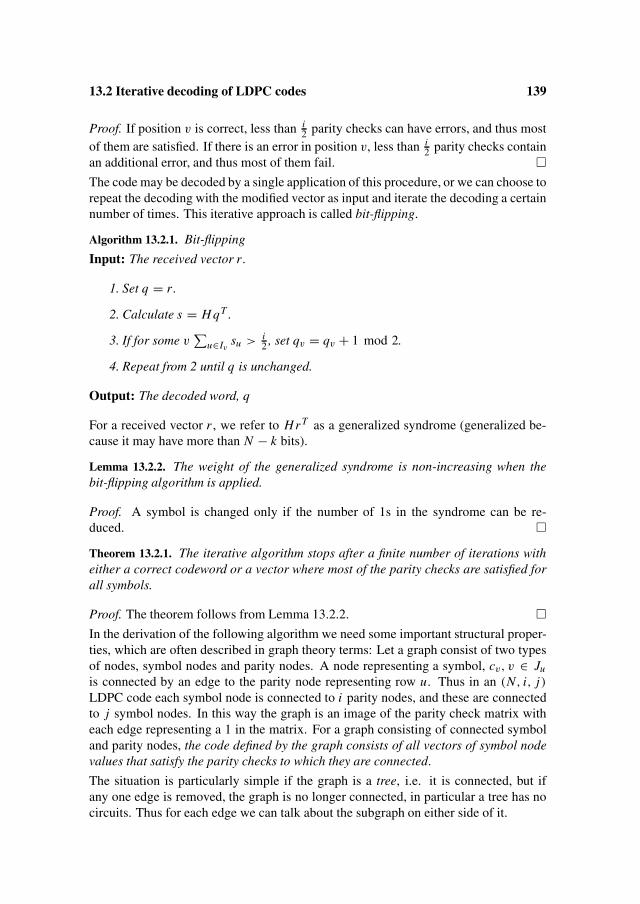
13.2 Iterative decoding of LDPC codes 139
Proof. If position v is correct, less than i2 parity checks can have errors, and thus most
of them are satisfied. If there is an error in position v, less than i2 parity checks contain
an additional error, and thus most of them fail. �The code may be decoded by a single application of this procedure, or we can choose torepeat the decoding with the modified vector as input and iterate the decoding a certainnumber of times. This iterative approach is called bit-flipping.
Algorithm 13.2.1. Bit-flipping
Input: The received vector r .
1. Set q = r .
2. Calculate s = H qT .
3. If for some v∑
u∈Iv su > i2 , set qv = qv + 1 mod 2.
4. Repeat from 2 until q is unchanged.
Output: The decoded word, q
For a received vector r , we refer to Hr T as a generalized syndrome (generalized be-cause it may have more than N − k bits).
Lemma 13.2.2. The weight of the generalized syndrome is non-increasing when thebit-flipping algorithm is applied.
Proof. A symbol is changed only if the number of 1s in the syndrome can be re-duced. �
Theorem 13.2.1. The iterative algorithm stops after a finite number of iterations witheither a correct codeword or a vector where most of the parity checks are satisfied forall symbols.
Proof. The theorem follows from Lemma 13.2.2. �In the derivation of the following algorithm we need some important structural proper-ties, which are often described in graph theory terms: Let a graph consist of two typesof nodes, symbol nodes and parity nodes. A node representing a symbol, cv, v ∈ Ju
is connected by an edge to the parity node representing row u. Thus in an (N, i, j)LDPC code each symbol node is connected to i parity nodes, and these are connectedto j symbol nodes. In this way the graph is an image of the parity check matrix witheach edge representing a 1 in the matrix. For a graph consisting of connected symboland parity nodes, the code defined by the graph consists of all vectors of symbol nodevalues that satisfy the parity checks to which they are connected.
The situation is particularly simple if the graph is a tree, i.e. it is connected, but ifany one edge is removed, the graph is no longer connected, in particular a tree has nocircuits. Thus for each edge we can talk about the subgraph on either side of it.
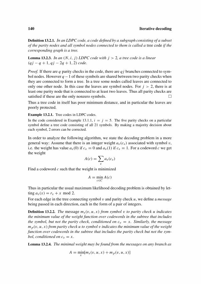
140 Iterative decoding
Definition 13.2.1. In an LDPC code, a code defined by a subgraph consisting of a subsetof the parity nodes and all symbol nodes connected to them is called a tree code if thecorresponding graph is a tree.
Lemma 13.2.3. In an (N, i, j) LDPC code with j > 2, a tree code is a linear(q j − q + 1, q j − 2q + 1, 2) code.
Proof. If there are q parity checks in the code, there are q j branches connected to sym-bol nodes. However q −1 of these symbols are shared between two parity checks whenthey are connected to form a tree. In a tree some nodes called leaves are connected toonly one other node. In this case the leaves are symbol nodes. For j > 2, there is atleast one parity node that is connected to at least two leaves. Thus all parity checks aresatisfied if these are the only nonzero symbols. �Thus a tree code in itself has poor minimum distance, and in particular the leaves arepoorly protected.
Example 13.2.1. Tree codes in LDPC codes.
In the code considered in Example 13.1.1, i = j = 5. The five parity checks on a particularsymbol define a tree code consisting of all 21 symbols. By making a majority decision abouteach symbol, 2 errors can be corrected.
In order to analyze the following algorithm, we state the decoding problem in a moregeneral way: Assume that there is an integer weight av(cv) associated with symbol v,i.e. the weight has value av(0) if cv = 0 and av(1) if cv = 1. For a codeword c we getthe weight
A(c) =∑v
av(cv)
Find a codeword c such that the weight is minimized
A = minc∈C
A(c)
Thus in particular the usual maximum likelihood decoding problem is obtained by let-ting av(x) = rv + x mod 2.
For each edge in the tree connecting symbol v and parity check u, we define a messagebeing passed in each direction, each in the form of a pair of integers.
Definition 13.2.2. The message ms(v, u, x) from symbol v to parity check u indicatesthe minimum value of the weight function over codewords in the subtree that includesthe symbol, but not the parity check, conditioned on cv = x. Similarly, the messagem p(v, u, x) from parity check u to symbol v indicates the minimum value of the weightfunction over codewords in the subtree that includes the parity check but not the sym-bol, conditioned on cv = x.
Lemma 13.2.4. The minimal weight may be found from the messages on any branch as
A = minx
[ms(v, u, x) + m p(v, u, x)]

13.2 Iterative decoding of LDPC codes 141
Proof. Each edge separates the tree into two subtrees, and the minimal weight is ob-tained by adding the contributions for the subtrees with one of the choices for cv = x .
�
Theorem 13.2.2. The messages defined in Definition 13.2.2 can be calculated recur-sively starting from the leaves of the tree. When all incoming messages to a node areknown, the outgoing messages are calculated as
1. Symbol node v,
ms(v, u′, x) = av(x) +∑
u∈Iv,u �=u′m p(v, u, x)
2. Parity node u,
m p(v′, u, x ′) =
∑v∈Ju,v �=v′
minx
ms(v, u, x)
when x ′ satisfies the parity check. For the other value of x ′, change one of thems such that the increase is minimal.
Proof. For a symbol node, the minimal value is the sum of the incoming values fromsubtrees connected to it plus the weight of the symbol itself. All of these values areconditioned on the same symbol value. For a parity node we first find the sum of theminimal incoming messages. The associated symbol values determines the possiblevalue on the output edge. In order to get the message for the other symbol value, wehave to change at least one input symbol. The smallest increase in the weight is ob-tained by changing only one message. In the first step we can calculate the messagesfrom those symbol nodes that are leaves in the tree, since the only input here are thesymbol weights av(cv). After each step, the new set of nodes that have all input mes-sages defined may be obtained as the leaves of the tree that remain when the leavesfrom the previous stage have been removed. �The minimal weight calculated from the messages is a lower bound on the number oferrors in the tree. Even though not all errors can be corrected with certainty, decodingthe tree code serves as a way of estimating the number of errors.
The messages can be simplified by always taking the difference between the two valuesrather than transmitting a pair of integers. This change has no effect on the result of thedecoding, but we lose information about the number of errors that is corrected. In thiscase the initial values of the weights are av = av(1) − av(0), i.e. ±1. The numericalvalue of the message difference indicates the reliability of the symbol. If all symbolweights are initiated to av(cv) and the outgoing messages are initially set to this value,we can use the updating from Theorem 13.2.2. By iterating this calculation a finitenumber of times, we arrive at the same result. The reason is that the message froma subtree does not depend on the incoming message, and thus the correct value willpropagate from the leaves as before.

142 Iterative decoding
If the symbol weights are initiated in the same way in a general graph, and the sameupdating rules are used, the messages in a given edge after s steps will depend on onlynodes that can be reached in s steps from this branch. If this part of the graph is a tree,the messages may be interpreted as for the tree code.
Algorithm 13.2.2. Iterative decoding by message-passing
Input: The received vector r
1. Initially the received symbols are assigned weights av(cv) = rv + 1 mod 2.
2. The messages are calculated as in Theorem 13.2.2.
3. The algorithm continues until the weights are unchanged or a preset limit on thenumber of iterations has been reached.
4. For each symbol, the value that gives the minimum number of errors is chosen.
Output: The decoded word q
The application of Algorithm 13.2.2 is only justified even in some approximate senseas long as the number of nodes that can be reached from a given starting node is lessthan N . If the difference messages av are used, they may be interpreted as reliabilitiesof the symbols and used in additional iterations of the algorithm. It can be observedexperimentally that the performance of the decoding is improved, but an exact analysisof this form of iterative decoding is difficult. However the following result indicatesthat it is sometimes possible to combine the local results of decoding the tree codesinto a global result:
Theorem 13.2.3. Assume that several tree codes in an LDPC code are decoded, and thatall N − k independent parity checks are included in the codes. If T is the largest num-ber of errors detected in the decoding of the tree codes, any error patterns of weight Twhich is consistent with the decoding results of the tree codes is an ML decision.
Proof. As discussed earlier, the minimal weight obtained by decoding a tree code is alower bound on the number of errors that has occurred, but there may be several possi-ble error patterns of the same weight. After decoding each code we can make a list ofthese patterns. Since the tree codes include all parity checks, an error pattern which isshared between all lists has the right syndrome. Since each tree code is decoded ML,the number of errors cannot be less than T . Thus any error pattern with T errors is ML,but there may not be such an error pattern. �
Example 13.2.2. A (15, 3, 3) LDPC code
The code considered in this example is the dual of the (15, 11, 3) Hamming code. We can geta generator matrix by removing the bottom row and the right (all 0s) column from the matrix inExample 1.2.3. The parity checks are weight 3 codewords of the Hamming code. There are 35such words, but we shall use a particular set of 15 words (of course only 11 of these are linearly
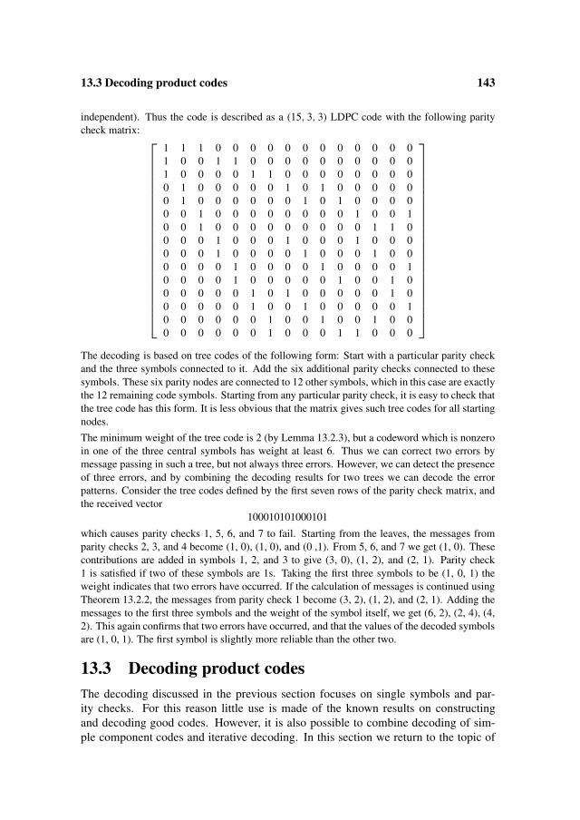
13.3 Decoding product codes 143
independent). Thus the code is described as a (15, 3, 3) LDPC code with the following paritycheck matrix:
1 1 1 0 0 0 0 0 0 0 0 0 0 0 01 0 0 1 1 0 0 0 0 0 0 0 0 0 01 0 0 0 0 1 1 0 0 0 0 0 0 0 00 1 0 0 0 0 0 1 0 1 0 0 0 0 00 1 0 0 0 0 0 0 1 0 1 0 0 0 00 0 1 0 0 0 0 0 0 0 0 1 0 0 10 0 1 0 0 0 0 0 0 0 0 0 1 1 00 0 0 1 0 0 0 1 0 0 0 1 0 0 00 0 0 1 0 0 0 0 1 0 0 0 1 0 00 0 0 0 1 0 0 0 0 1 0 0 0 0 10 0 0 0 1 0 0 0 0 0 1 0 0 1 00 0 0 0 0 1 0 1 0 0 0 0 0 1 00 0 0 0 0 1 0 0 1 0 0 0 0 0 10 0 0 0 0 0 1 0 0 1 0 0 1 0 00 0 0 0 0 0 1 0 0 0 1 1 0 0 0
The decoding is based on tree codes of the following form: Start with a particular parity checkand the three symbols connected to it. Add the six additional parity checks connected to thesesymbols. These six parity nodes are connected to 12 other symbols, which in this case are exactlythe 12 remaining code symbols. Starting from any particular parity check, it is easy to check thatthe tree code has this form. It is less obvious that the matrix gives such tree codes for all startingnodes.
The minimum weight of the tree code is 2 (by Lemma 13.2.3), but a codeword which is nonzeroin one of the three central symbols has weight at least 6. Thus we can correct two errors bymessage passing in such a tree, but not always three errors. However, we can detect the presenceof three errors, and by combining the decoding results for two trees we can decode the errorpatterns. Consider the tree codes defined by the first seven rows of the parity check matrix, andthe received vector
100010101000101
which causes parity checks 1, 5, 6, and 7 to fail. Starting from the leaves, the messages fromparity checks 2, 3, and 4 become (1, 0), (1, 0), and (0 ,1). From 5, 6, and 7 we get (1, 0). Thesecontributions are added in symbols 1, 2, and 3 to give (3, 0), (1, 2), and (2, 1). Parity check1 is satisfied if two of these symbols are 1s. Taking the first three symbols to be (1, 0, 1) theweight indicates that two errors have occurred. If the calculation of messages is continued usingTheorem 13.2.2, the messages from parity check 1 become (3, 2), (1, 2), and (2, 1). Adding themessages to the first three symbols and the weight of the symbol itself, we get (6, 2), (2, 4), (4,2). This again confirms that two errors have occurred, and that the values of the decoded symbolsare (1, 0, 1). The first symbol is slightly more reliable than the other two.
13.3 Decoding product codesThe decoding discussed in the previous section focuses on single symbols and par-ity checks. For this reason little use is made of the known results on constructingand decoding good codes. However, it is also possible to combine decoding of sim-ple component codes and iterative decoding. In this section we return to the topic of

144 Iterative decoding
decoding product block codes, and the following section discusses iterative decodingusing convolutional codes.
The basic properties of product codes were introduced in Section 10.1, and we notedthat it was desirable to correct a number of errors significantly greater than D
2 .
We introduce a graph terminology similar to the one in the previous section by associat-ing a node with each symbol and a parity node with each row and column. Each symbolnode is connected to the parity node for the respective row and column. Thus the paritynode represents not just a single parity check, but a decoding of the component code.
Definition 13.3.1. In a product code, a code defined by a subgraph consisting of theparity node for a row and all column nodes and symbol nodes is called a row treecode. Similarly a column tree code is defined by one column node, all row nodes andall symbol nodes.
It may be readily checked that the graphs in question are in fact trees.
In order to decode the first row tree code we decode each column twice. We decodecolumn j assuming that the symbol in the first row is 0; the number of errors correctedin this case is a j (0). Similarly a j (1) is the number of errors corrected when the firstsymbol is assumed to be 1. Using these weights we find a codeword in row 1, c1, suchthat the sum of the weights is minimized:
A = min∑c∈C
a j (c1 j )
Lemma 13.3.1. For any error pattern of weight less than D2 the first row is correctly
decoded.
Proof. Any codeword in the row tree code that has a nonzero symbol in the first row,has weight at least d in that row, and total weight at least D = d2. Thus if the numberof errors is less than D
2 , any codeword with a different bit in the first row would havedistance greater than D
2 to the received vector. However, since there are codewordsof weight d which are nonzero only in a single column (and outside row 1), the errorpattern is not necessarily correct in other rows. �We can now prove a result similar to Theorem 13.2.3.
Theorem 13.3.1. Let a row tree code and a column tree code in a product code be de-coded, and the total number of errors be T in both cases. Any error pattern of weightT which is consistent with both results is maximum likelihood.
Proof. All parity nodes are included in the two codes, and by the same reasoning asin the proof of Theorem 13.2.3 any error pattern that is consistent with the results ofdecoding the two codes is maximum likelihood. �

13.4 Parallel concatenation of convolutional codes (‘turbo codes’) 145
Example 13.3.1. Decoding of product code
We consider a product of two extended Hamming codes defined by the parity check matrix givenin Example 1.2.3. Thus the parameters of the code are (256, 121, 16). As a first step of the de-coding we calculate the syndromes of all rows and columns. The syndrome of a single Hammingcode may be expressed as xp, where p is 0 for an even number of errors and 1 for error patternsof odd weight, and x is the mod 2 sum of the error positions. In order to simplify the examplewe consider a case where the rows and columns have the same sequence of syndromes (the errorpattern otherwise has a typical distribution on rows and columns):
(01, 20, 31, 20, 51, 41, 150, 71, 91, 00, 00, 00, 00, 00, 00, 31)
Since there is at least one error in the odd columns and two errors in even syndromes withnonzero syndromes, the syndromes indicate at lest 13 errors. We shall base the decoding on twotree codes, the row 0 code with messages from all columns and the corresponding column 0 code.The messages may be described in the following simplified way when only a single iteration isused:
00: 0 errors if the symbol is correct, four errors otherwisex0: two errors whether the symbol is correct or in error01: one error if the symbol is an errors, three otherwisex1: three errors if the symbol is an error, one otherwise
Given these messages we search for the minimum weight codeword in row 0, which has syn-drome 31. We shall not give a formal decoding algorithm for the extended Hamming code withweights associated with the symbols, but based on the decoding of the row without weights, weshall find a nearby codeword which minimizes the sum of the weights. In addition to the zerocodeword we consider low weight codewords with 1s among the positions 1, 2, 4, and 7 wherethe columns indicate a single error in row 0 or a double error. Adding a 1 in position 3 to givethe correct syndrome we get the potential error patterns
1 1 0 0 0 0 0 0 0 0 0 0 0 0 0 10 0 0 1 0 0 1 0 0 0 0 0 0 0 0 11 1 1 1 0 0 1 0 0 0 0 0 0 0 0 0
Of these the second pattern gives at least 17 errors, whereas the two other patterns could give 15errors. While these results give codewords in the tree codes, they may not produce codewords inthe product code. The third error pattern would place the double errors in columns 2 and 4 in rows0 and 2, but this is not consistent with the syndrome in row 2. By the symmetry of the syndromes,the remaining solution is also the unique minimum weight codeword in the column 0 tree code.The single errors in rows/columns 3, 5, and 9 are in immediate agreement. The remainingsingle and double errors in rows/columns 4, 6, 7, and 8 are seen to agree if placed in positions(4, 4), (4, 6), (6, 4), (7, 7), (7, 8), and (8, 7). Since the two tree codes agree, the decoding is ML.
13.4 Parallel concatenation of convolutional codes(‘turbo codes’)
In parallel encoding the same information symbols are encoded by two systematic en-coders, and the transmitted frame consists of the information symbols and two sets ofparity symbols. Usually the information symbols are permuted in some way before
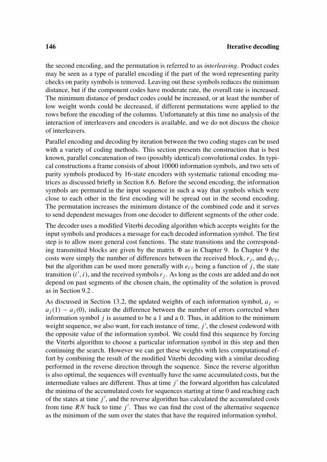
146 Iterative decoding
the second encoding, and the permutation is referred to as interleaving. Product codesmay be seen as a type of parallel encoding if the part of the word representing paritychecks on parity symbols is removed. Leaving out these symbols reduces the minimumdistance, but if the component codes have moderate rate, the overall rate is increased.The minimum distance of product codes could be increased, or at least the number oflow weight words could be decreased, if different permutations were applied to therows before the encoding of the columns. Unfortunately at this time no analysis of theinteraction of interleavers and encoders is available, and we do not discuss the choiceof interleavers.
Parallel encoding and decoding by iteration between the two coding stages can be usedwith a variety of coding methods. This section presents the construction that is bestknown, parallel concatenation of two (possibly identical) convolutional codes. In typi-cal constructions a frame consists of about 10000 information symbols, and two sets ofparity symbols produced by 16-state encoders with systematic rational encoding ma-trices as discussed briefly in Section 8.6. Before the second encoding, the informationsymbols are permuted in the input sequence in such a way that symbols which wereclose to each other in the first encoding will be spread out in the second encoding.The permutation increases the minimum distance of the combined code and it servesto send dependent messages from one decoder to different segments of the other code.
The decoder uses a modified Viterbi decoding algorithm which accepts weights for theinput symbols and produces a message for each decoded information symbol. The firststep is to allow more general cost functions. The state transitions and the correspond-ing transmitted blocks are given by the matrix as in Chapter 9. In Chapter 9 thecosts were simply the number of differences between the received block, r j , and φi ′ i ,but the algorithm can be used more generally with ei ′ i being a function of j , the statetransition (i ′, i), and the received symbols r j . As long as the costs are added and do notdepend on past segments of the chosen chain, the optimality of the solution is provedas in Section 9.2 .
As discussed in Section 13.2, the updated weights of each information symbol, a j =a j (1) − a j (0), indicate the difference between the number of errors corrected wheninformation symbol j is assumed to be a 1 and a 0. Thus, in addition to the minimumweight sequence, we also want, for each instance of time, j ′, the closest codeword withthe opposite value of the information symbol. We could find this sequence by forcingthe Viterbi algorithm to choose a particular information symbol in this step and thencontinuing the search. However we can get these weights with less computational ef-fort by combining the result of the modified Viterbi decoding with a similar decodingperformed in the reverse direction through the sequence. Since the reverse algorithmis also optimal, the sequences will eventually have the same accumulated costs, but theintermediate values are different. Thus at time j ′ the forward algorithm has calculatedthe minima of the accumulated costs for sequences starting at time 0 and reaching eachof the states at time j ′, and the reverse algorithm has calculated the accumulated costsfrom time RN back to time j ′. Thus we can find the cost of the alternative sequenceas the minimum of the sum over the states that have the required information symbol.

13.4 Parallel concatenation of convolutional codes (‘turbo codes’) 147
The messages from code 1 about information symbol u j , m1( j)) is now calculated asa j − m2( j), where m2 is the message received from code 2.
Algorithm 13.4.1. Turbo decoding
Input: The received sequence
1. Decode code 1 using the modified Viterbi algorithm with weights
ei ′i ( j) = W (φi ′ i + r j )
if the information symbol ui ′ i = 0,
ei ′ i ( j) = W (φi ′ i + r j ) + m2( j)
if the information symbol ui ′ i = 1.
2. Repeat the decoding in the reverse direction to obtain the accumulated weightsµ′
i ( j).
3. For each j ′, find the new weight of the information symbol at time j ′, a j ′ as thedifference between the weight of the ML sequence and the best sequence with theopposite value of the information symbol at time j ′.
4. Generate a message for each information symbol as m1( j ′) = a j ′ − m2( j ′).
5. Permute the information symbols and decode code 2 using these messages.
6. Iterate between the two decoding steps a prescribed number of times.
Output: The decoded information sequence
The rationale for Algorithm 13.4.1 is that decoding decisions in a convolutional codeusually depend on only a short segment of the received sequence. Thus the weightof an information symbol may be interpreted as the difference in weight between twodecoded sequences that differ only on a segment close to the symbol. The purpose ofthe interleaver is to ensure that the messages contributing to the decision come fromdifferent parts of the frame and are based on independent decoding decisions. If theframe is large and only a limited number of iterations are used, the decoding will in thisway approximately have the properties of decoding a tree code. However, the numberof iterations is often about 20, and tree code approximation is no longer valid. As formessage passing decoding of LDPC codes we may interpret the later iterations as at-tempts to reconcile the decoding results for the two convolutional codes by assigningreliabilities of the information symbols. However, a precise analysis of the algorithmhas not been made.
Example 13.4.1. Turbo decoding.
In this example we illustrate the decoding principle by considering a very small parallel encod-ing. A systematic convolutional code of rate 1
2 and memory 1 is generated by g = (11.01). A

148 Iterative decoding
tail-biting version of length 5 is used here. If the information bits are reordered to the sequence(1, 3, 5, 2, 4), and encoded again with the same code, we may represent the total rate 1
3 code bythe generator matrix
1 0 0 0 0 1 1 0 0 0 1 1 0 0 00 1 0 0 0 0 1 1 0 0 0 0 1 1 00 0 1 0 0 0 0 1 1 0 1 0 0 0 10 0 0 1 0 0 0 0 1 1 0 1 1 0 00 0 0 0 1 1 0 0 0 1 0 0 0 1 1
Thus the code is a (15, 5, 5) block code. The codeword is (11000, 10100, 11110) and the re-ceived sequence (01000, 10000, 01110). We iterate between decoding the two tail-biting codes.
The first decoding operates on the received sequence 01.10.00.00.00. Starting and ending instate 0 we get the costs [
0 1 2 2 2 2− 1 1 2 3 −
]
There are two equally good decisions, and we choose the zero word. Decoding the same se-quence in the reverse direction we get the costs
[2 1 0 0 0 0− 1 1 1 1 −
]
Thus for the information symbols (0, 0, 0, 0, 0) the costs are (2, 2, 2, 2, 2), while a 1 in each ofthe first four positions gives weights that are the sums of the costs in state 1: (2, 2, 3, 4, 3). Wehave added the weight of the last information bit without a detailed calculation. This result showsthat the information sequence (1, 1, 0, 0, 0) has the same number of errors as the zero sequence,whereas more errors would have to be assumed to make the other information bits 1s. Takingthe difference between the two sets of weights we get
a( j) = (0, 0, 1, 2, 1)
The messages are obtained by subtracting the contribution from the current information symbol:
µ1( j) = (−1, 1, 0, 1, 0)
Now the second code is decoded with the received sequence 00.01.11.01.00. In the decoding,the messages from the first decoding stages are added to the cost of the transitions where theinformation symbol is a 1. However the messages have to be permuted in the same way as theinformation symbols.
Again starting in state 0 the costs become[
0 0 1 3 2 2− 1 2 2 4 −
]
and in the reverse direction [2 2 1 1 0 0− 1 2 0 1 −
]
This gives messagesµ2( j) = (0, 0, −3, 2, 2)
Thus, when the decoding of the first code is repeated, the message −3 decides the second bit infavor of a 1, and the decoded information sequence becomes (1, 1, 0, 0, 0).
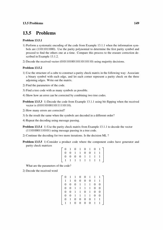
13.5 Problems 149
13.5 ProblemsProblem 13.5.1
1) Perform a systematic encoding of the code from Example 13.1.1 when the information sym-bols are (11011011000). Use the parity polynomial to determine the first parity symbol andproceed to find the others one at a time. Compare this process to the erasure correction de-scribed in Example 13.1.2.
2) Decode the received vector (010110100110110110110) using majority decisions.
Problem 13.5.2
1) Use the structure of a cube to construct a parity check matrix in the following way: Associatea binary symbol with each edge, and let each corner represent a parity check on the threeadjoining edges. Write out the matrix.
2) Find the parameters of the code.
3) Find a tree code with as many symbols as possible.
4) Show how an error can be corrected by combining two tree codes.
Problem 13.5.3 1) Decode the code from Example 13.1.1 using bit flipping when the receivedvector is (010110100110111110110).
2) How many errors are corrected?
3) Is the result the same when the symbols are decoded in a different order?
4) Repeat the decoding using message passing.
Problem 13.5.4 1) Use the parity check matrix from Example 13.1.1 to decode the vector(111010001110101) using message passing in a tree code.
2) Continue the decoding for two more iterations. Is the decision ML ?
Problem 13.5.5 1) Consider a product code where the component codes have generator andparity check matrices
0 1 0 1 0 1 0 10 0 1 1 0 0 1 10 0 0 0 1 1 1 11 1 1 1 1 1 1 1
What are the parameters of the code?
2) Decode the received word
0 1 1 0 0 1 1 11 1 0 0 0 0 1 10 0 0 1 1 1 0 00 0 1 1 1 1 0 00 0 1 1 0 1 0 00 0 1 1 1 1 0 00 1 0 0 0 0 1 11 1 0 0 0 0 1 1

Chapter 14
Algebraic geometry codes
In this chapter we briefly describe a class of algebraic block codes, which is a recentgeneralization of Reed-Solomon codes.
Where Reed-Solomon codes over Fq can have length at most q , these so called alge-braic geometry codes can be significantly longer. We will not give the general theoryhere but we present a special class of codes that seems to have the best chance to even-tually be used in practice.
14.1 Hermitian codesA codeword in an (n, k) Reed-Solomon code is obtained by evaluating certain functions(polynomials from Fq [x] of degree smaller than k) in certain elements (x1, x2, . . . , xn)from Fq . In particular we can get a basis for the code by evaluating the monomials1, x, . . . , xk−1 in the n elements.
The algebraic geometry codes are obtained by generalizing this idea in the sense thatone chooses points from some geometric object (i.e. curves or higher dimensionalsurfaces) and then chooses a suitable set of functions. The evaluation of any of thesefunctions in the chosen points gives a codeword. It turns out that with the proper choiceof points and functions one gets codes (for large q and n) that are better than previouslyknown codes.
In order to describe the codes we need some facts on polynomials in two variables. LetF be a field, then F[x, y] denotes the set of polynomials in the variables x and y withcoefficients from F , i.e. expressions of the form
am,nxm yn + · · · + ai, j x i y j + · · · + a0,1y + a1,0x + a0,0
where ai, j ∈ F . The degree is the maximum of the numbers i + j with ai, j �= 0. Likepolynomials in one variable a polynomial in two variables is irreducible if it cannot bewritten as a product of polynomials of positive degree.
We state without proof a theorem that plays the same role as Theorem 2.2.2 did forReed-Solomon codes.
152 Algebraic geometry codes
Theorem 14.1.1. (Bezout) Let f (x, y), g(x, y) ∈ F[x, y] where f (x, y) is irreducibleand has degree m, and g(x, y) has degree n. If g(x, y) is not a multiple of f (x, y),then the two polynomials have at most mn common zeroes in F2.
In the following we will describe some algebraic geometric codes, the Hermitian codes.The construction consists of choosing points on a specific curve and then choosing asuitable set of functions whose values in these points give a codeword. This illustratesthe general construction.
We choose points P1 = (x1, y1), P2 = (x2, y2), . . . , Pn = (xn, yn) as all the differentelements of 2Fq2 that satisfy the equation
xq+1 − yq − y = 0
It can be shown (see Problem 14.3.3) that the polynomial xq+1 − yq − y is irreducible.
Note that the points have coordinates in Fq2 . With the notation as above we have:
Lemma 14.1.1. n = q3.
The points are (0, β) with β ∈ Fq2, βq + β = 0
and(αi(q+1)+ j (q−1), βi
), i = 0, 1, . . . , q − 2, j = 0, 1, . . . , q,
where βiq + βi = αi(q+1), βi ∈ Fq2 and α is a primitive element of Fq2 .
Proof. We first note that if β ∈ Fq2 , then βq + β ∈ Fq . Also βq1 + β1 = β
q2 + β2 ⇒
βq1 − β
q2 + β1 − β2 = 0 and therefore (β1 − β2)
q + (β1 − β2) = 0. The polynomialxq + x has exactly q zeroes in Fq2 (see Problem 14.3.4), so βq + β = 0 in q cases and
for each i ∈ {0, 1, . . . , q −2}, βq +β = αi(q+1) in q cases, since αq+1 is a primitiveelement of Fq . In the first case we get xq+1 = 0 and hence x = 0 and in the secondcase we get xq+1 = αi(q+1) with the q + 1 solutions αi+ j (q−1), j = 0, 1, . . . , q.
Therefore the number of points n = q + (q2 − q)(q + 1) = q3. �In order to describe the set of functions we will use in the construction of the codes,we introduce the following:
Definition 14.1.1. For xa yb ∈ Fq2[x, y] let
ρ(xa yb) = aq + b(q + 1)
and for f (x, y) = ∑i, j fi, j x i y j ∈ Fq2[x, y],
ρ ( f (x, y)) = maxfi, j �=0
ρ(
xi y j)
The function ρ : Fq2[x, y] is called the order function.
We note that ρ( f (x, y)g(x, y)) = ρ( f (x, y)) + ρ(g(x, y)).
With this we define the Hermitian codes.
14.1 Hermitian codes 153
Definition 14.1.2. Let s be a natural number s < n − q2 + q. A Hermitian code H (s)over Fq2 consists of the codewords
( f (P1), f (P2), . . . , f (Pn))
where f (x, y) ∈ Fq2[x, y] with ρ( f (x, y)) ≤ s and degx ( f (x, y)) < q + 1
From the construction it is obvious that the length of the code is n, and it is also clearthat the code is linear.
To determine the dimension we first note that the evaluation of the monomials
M(s) = {xa yb where 0 ≤ ρ(
xa yb)
≤ s, 0 ≤ a < q + 1}
in P1, P2, . . . , Pn gives a basis for the code. To see this we first prove
Lemma 14.1.2. The elements of M(s) have different orders.
Proof. If
ρ(
xa1 yb1)
= ρ(
xa2 yb2)
we have a1q + b1(q + 1) = a2q + b2(q + 1) and therefore
(a1 − a2 + b1 − b2)(q + 1) = (a1 − a2). But the absolute value of the right- hand sideis smaller than q + 1 and therefore we must have a1 = a2 and hence b1 = b2. �This in turn also implies that we have a natural ordering of these monomials namelyby their ρ value. Let this be φ0, φ1, . . . .
Lemma 14.1.3. The vectors obtained by evaluating the monomials in M(s) in the pointsP1, P2, . . . , Pn are linearly independent.
Proof. Suppose that λ0φ0(Pj ) + · · · + λvφv(Pj ) = 0 for j = 1, 2, . . . , n.
This implies that the polynomial φ(x, y) = λ0φ0(x, y) + · · · + λvφv(x, y) has n ze-roes. Since degx(φ(x, y)) < q + 1 it is not a multiple of xq+1 − yq − y and the degreeof φ(x, y) is at most s+q
q+1 and since P1, P2, . . . , Pn are points on the curve with the
equation xq+1 − yq − y = 0 which has degree q + 1 it follows from Theorem 14.1.1that the number of zeroes is at most s + q . But s + q < n and therefore λ0φ0(x, y) +· · · + λvφv(x, y) must be the zero polynomial so λ0 = λ1 = · · · = λv = 0. �Let µ(s) denote the number of elements in M(s).
We then have
Theorem 14.1.2. If s > q2 − q − 2, then µ(s) = s + 1 − q2−q2 and for s > q2 − q − 1
there exists (a, b) with 0 ≤ a ≤ q, 0 ≤ b such that aq + b(q + 1) = s.
Proof. By induction on s. If s = q2 − q − 1 the number of solutions to the inequality
that has a = j is q − 1 − j so the total number is q2−q2 corresponding to the statement

154 Algebraic geometry codes
of the theorem. If s = q2 − q , then (q − 1)q = s. Suppose we have proven thestatement for all s∗ where q2 − q ≤ s∗ < s. Then if a1q + b1(q + 1) = s − 1 we get(a1 − 1)q + (b1 + 1)(q + 1) = s. If a1 = 0 we get s = q · q + (b1 + 1 − q). �This combined with the observation above immediately gives
Theorem 14.1.3. The dimension k(s) of the code H (s) is
k(s) ={
µ(s) if 0 ≤ s ≤ q2 − q − 2
s + 1 − q2−q2 if q2 − q − 2 < s < n − q2 + q
The number g = 12 (q2 − q) is called the genus of the curve xq+1 − yq − y = 0. It can
be proved that this is the number of natural numbers that do not appear as orders. Wealso have
Theorem 14.1.4. H (s)⊥ = H (n + q2 − q − 2 − s).
Proof. We will only prove the theorem in the case where s > q2 − q − 2. From theabove it is easy to see that k(s) + k(n + q2 − q − 2 − s) = n, so it suffices to provethat any element of H (s) is orthogonal to any element of H (n + q2 − q − 2 − s).
This is the same as showing that if (a1, b1) and (a2, b2) satisfy a1q + b1(q + 1) ≤s, a1 < q + 1 and a2q + b2(q + 1) ≤ n + q2 − q − 2 − s, a2 < q + 1 then,
n∑i=0
xa1+a2 yb1+b2(Pi ) = 0
By Lemma 14.1.1 the left- hand side of this equation is the same as
∑βq+β=0
0a1+a2βb1+b2 +q−2∑i=0
∑
βq+β=αi(q+1)
βb1+b2
q∑j=0
(αi(q+1)+ j (q−1))a1+a2
If a1 + a2 = 0 this is ∑βb1+b2 = 0
If a1 + a2 �= 0 we get
q−2∑i=0
α j (q−1)(a1+a2)∑
βq+β=αi(q+1)
βb1+b2
q∑j=0
α j (q−1)(a1+a2)
Sinceq∑
j=0
α j (q−1)(a1+a2) = α(q2−1)(a1+a2) − 1
α(q−1)(a1+a2) − 1
the sum is 0 if α(q−1)(a1+a2) �= 1.
The case α(q−1)(a1+a2) = 1 is treated in Problem 14.3.5.

14.2 Decoding Hermitian codes 155
Note that it is now easy to get a parity check matrix for the code H (s). The rowsof that are the evaluation of the monomials in M(n + q2 − q − 2 − s) in the pointsP1, P2, . . . , Pn .
Our final task is to estimate the minimum distance of the Hermitian codes. Here wehave the following
Theorem 14.1.5. Let d(s) denote the minimum distance of the code H (s).
If q2 − q − 2 < s < n − q2 + q, then d(s) ≥ n − s
We will only prove this in the case where s = h(q +1) for some nonnegative integer h.We can show that a codeword ( f (P1), . . . , f (Pn)) in H (s) has weight at least n − s byshowing that the polynomial f (x, y) has at most s zeroes among the points P1, . . . , Pn .Since aq + b(q + 1) ≤ h(q + 1) we get (a + b)(q + 1) ≤ h(q + 1) + q and hencea + b ≤ h + q
q+1 and therefore a + b ≤ h, so the degree of f (x, y) is at most h. Wealso have that degx ( f (x, y)) < q + 1 and therefore by Theorem 14.1.1 f (x, y) has atmost h(q + 1) = s zeroes, since P1, P2, . . . , Pn are on a curve of degree q+1. �A proof of the theorem for other values of s is more difficult, actually one can provethat d(s) = n − s.
Combining Theorem 14.1.3 and Theorem 14.1.5 we get
Corollary 14.1.1. d(s) ≥ n − k(s) + 1 − g for the codes H (s).
Recall that for Reed-Solomon codes we have d = n − k + 1 so the algebraic geometrycodes have smaller minimum distance, but are longer.
Example 14.1.1. Hermitian codes over F16
With q = 4 we get (64, s + 1 − 6, 64 − s) codes over F16 for s = 10, 11, . . . , 50. If we take the(64, 32, 27) code over F16 and concatenate it with the (8,4,4) extended Hamming code we get a(512,128,108) binary code.
14.2 Decoding Hermitian codesIn this section we will present a mixture of the methods from Section 5.2 and Section5.4 to give a decoding algorithm for Hermitian codes.
We consider the code H (s) as presented in Section 14.1 and receive a word r =(r1, r2, . . . , rn) which is the sum of a codeword c = ( f (P1), f (P2), . . . , f (Pn)) andan error vector e of weight τ . The idea is to determine a polynomial in three variables
Q(x, y, z) = Q0(x, y) + z Q1(x, y) ∈ Fq2[x, y, z]\{0}
1. Q(xi , yi , ri ) = 0, i = 1, . . . , n.
2. ρ(Q0) ≤ s + τ + g.
3. ρ(Q1) ≤ τ + g.

156 Algebraic geometry codes
Theorem 14.2.1. If τ errors occurred, then there is at least one nonzero polynomialQ(x, y, z) which satisfies the three conditions.
Proof. If there are τ errors, there exists a polynomial Q1(x, y) = ∑τi=0 λiφi with
the error positions as zeroes since we get a system of τ homogenous linear equationsin τ + 1 unknowns. If f (x, y) is the polynomial that gives the transmitted code-word, and r(x, y) is the polynomial corresponding to the received word we then havef (Pj )Q1(Pj ) = r(Pj )Q1(Pj ) for j = 1, 2, . . . , n since f (Pj ) = r(Pj ) if Pj isnot an error position and Q1(Pj ) = 0 if Pj is an error position. This means thatQ(x, y, z) = f (x, y)Q1(x, y) − z Q1(x, y) satisfies all three conditions. �
Theorem 14.2.2. If the number of errors is less than d−g2 , then the error postions are
zeroes of Q1(x, y).
Proof. If τ <d−g
2 = n−s−g2 we get s+τ+g < n−τ . The polynomial Q(x, y, f (x, y)),
where the transmitted codeword is generated by f (x, y) has at least n−τ zeroes amongthe points P1, P2, . . . , Pn . The degree of Q(x, y, f (x, y)) is smaller than or equal tos+τ+g
q+1 so by Theorem 14.1.1 it must either be the zero polynomial or a multiple of the
polynomial xq+1 − yq − y. In both cases we get Q0(Pj ) + f (Pj )Q1(Pj ) = 0 forj = 1, 2, . . . , n. Since we have Q0(Pj ) + r(Pj )Q1(Pj ) = 0 for j = 1, 2, . . . , n,we get by subtraction (r(Pj ) − f (Pj ))Q1(Pj ) = 0 for j = 1, 2, . . . , n and henceQ1(Pj ) = 0 if Pj is an error position. �From the above we can now give a decoding algorithm for the codes H (s). We definel0 = s + � d−g
2 � and l1 = � d−g2 �.
The algorithm now can be presented as follows:
Algorithm 14.2.1.
Input: A received word r = (r1, r2, . . . , rn)
1. Solve the system of linear equations
φ0(P1) φ1(P1) . . . φl0(P1) r1φ0(P1) r1φ1(P1) . . . r1φl1
(P1)
φ0(P2) φ1(P2) . . . φl0(P2) r2φ0(P2) r2φ1(P2) . . . r2φl1
(P2)
.
.
.
.
.
.
.
.
.
.
.
.
.
.
.
.
.
.
.
.
.
.
.
.φ0(Pn ) φ1(Pn ) . . . φl0
(Pn ) rnφ0(Pn ) rn φ1(Pn ) . . . rn φl1(Pn )
Q0,0Q0,1Q0,2
.
.
.Q0,l0Q1,0Q1,1
.
.
.Q1,l1
=
000
.
.
.000
.
.
.0
2. Put Q1(x, y) = ∑l1j=0 Q1, jφ j .
3. Find the zeroes of Q1(x, y) among the points P1, P2, . . . , Pn.
4. Calculate the first l1 + g −1 syndromes using the parity check matrix of the codeand the received word.

14.3 Problems 157
5. Solve the system of linear equations using the parity check matrix and the (pos-sible) error positions and the calculated syndromes to find the error values.
output: The error vector
Notice in the system above that each row of the matrix corresponds to a triple (xi ,yi ,ri ).We have already seen that if the number of errors is smaller than d−g
2 , then the outputof the algorithm is the sent word.
Example 14.2.1. Decoding of the code H(27) over F16.
The code has parameters (64, 22, 37) and the above algorithm corrects 15 errors.
It is possible to present another version of the above algorithm as we did in Section5.4 and generalize it so that all error patterns of weight smaller than half the minimumdistance can be decoded; we refer to the special literature for that.
14.3 ProblemsProblem 14.3.1
1) With s = 27 what are the parameters of the code H(s) over F16?
2) Find a generator matrix for the code.
3) What are the parameters of the dual code?
4) How can you find a parity check matrix of the code?
Problem 14.3.2 (Project) Write a program that implements the decoding algorithm for the codesH(s) over F16.
Try to decode random error patterns of weight up to half the minimum distance.
Problem 14.3.3 Show that the polynomial xq+1 − yq − y is irreducible in Fq2 [x, y].Hint: write xq+1 − yq − y as (a(x) + yb(x, y)) · (c(x) + yd(x, y)).
Problem 14.3.4 Show that the polynomial xq + x has exactly q zeroes in Fq2 .
Problem 14.3.5 Complete the proof of Theorem 14.1.4 by considering the case whenα(q−1)(a1+a2) = 1.

Appendix A
Communication channels
In some communication channels the output is accurately described as the sum of (ascaled version of) the input and an independent noise term, which follows a Gaussiandistribution. This description applies to deep space communication where several cod-ing techniques were first applied. The appendix describes how the codes studied in thisbook are applied to such channels, and how some of the decoding techniques can bemodified to work in this context.
A.1 Gaussian channelsThe concept of mutual information as introduced in Chapter 4 can be extended to realvariables. We define the mutual information by a modification of (4.2)
I (X; Y ) = E
[log
p(y|x)
p(y)
](A.1)
where p is the density function. Note that for a ratio between two probabilities, wemay use the ratio of the density function. Again the capacity is the maximum of thisquantity with respect to an acceptable input distribution. We shall consider only thespecial case that is of practical importance:
Definition A.1.1. A discrete time memoryless additive Gaussian channel is defined byvariables X and Y , where X has zero mean and standard deviation σ , and Y = X + Nwhere the noise variable N is normal with zero mean and standard deviation ρ andindependent of X.
We note without proof that the mutual information is maximized by choosing Y tobe Gaussian, and that this implies X Gaussian. With this choice the capacity may becalculated.
Theorem A.1.1. The capacity of the discrete memoryless Gaussian channel is
C = 1
2log
(1 + σ 2
ρ2
)(A.2)
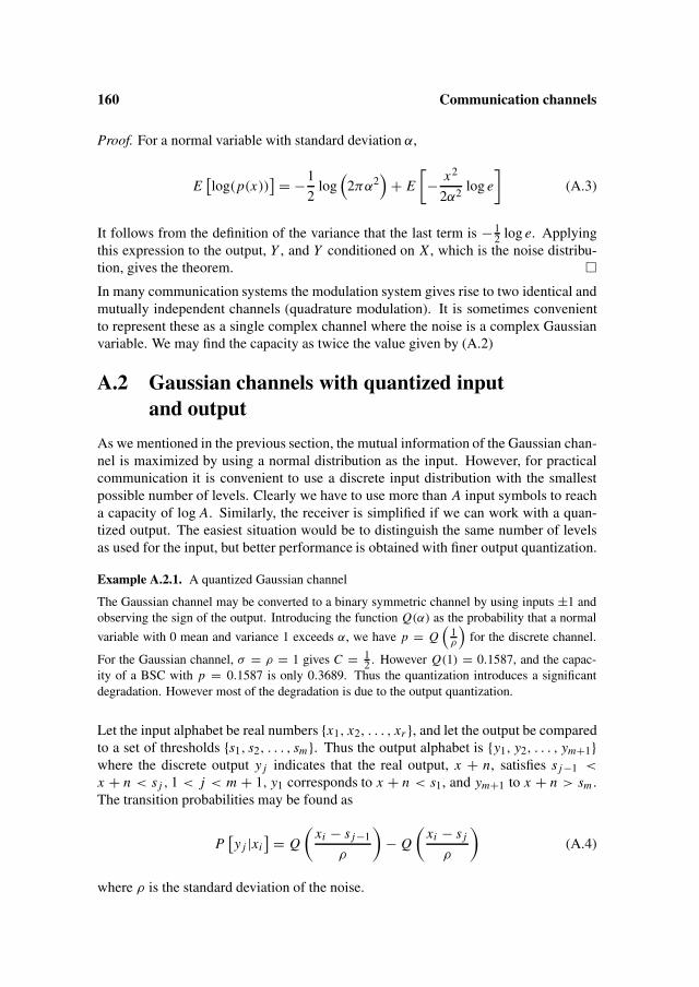
160 Communication channels
Proof. For a normal variable with standard deviation α,
E[log(p(x))
] = −1
2log
(2πα2
)+ E
[− x2
2α2log e
](A.3)
It follows from the definition of the variance that the last term is − 12 log e. Applying
this expression to the output, Y , and Y conditioned on X , which is the noise distribu-tion, gives the theorem. �In many communication systems the modulation system gives rise to two identical andmutually independent channels (quadrature modulation). It is sometimes convenientto represent these as a single complex channel where the noise is a complex Gaussianvariable. We may find the capacity as twice the value given by (A.2)
A.2 Gaussian channels with quantized inputand output
As we mentioned in the previous section, the mutual information of the Gaussian chan-nel is maximized by using a normal distribution as the input. However, for practicalcommunication it is convenient to use a discrete input distribution with the smallestpossible number of levels. Clearly we have to use more than A input symbols to reacha capacity of log A. Similarly, the receiver is simplified if we can work with a quan-tized output. The easiest situation would be to distinguish the same number of levelsas used for the input, but better performance is obtained with finer output quantization.
Example A.2.1. A quantized Gaussian channel
The Gaussian channel may be converted to a binary symmetric channel by using inputs ±1 andobserving the sign of the output. Introducing the function Q(α) as the probability that a normal
variable with 0 mean and variance 1 exceeds α, we have p = Q(
1ρ
)for the discrete channel.
For the Gaussian channel, σ = ρ = 1 gives C = 12 . However Q(1) = 0.1587, and the capac-
ity of a BSC with p = 0.1587 is only 0.3689. Thus the quantization introduces a significantdegradation. However most of the degradation is due to the output quantization.
Let the input alphabet be real numbers {x1, x2, . . . , xr }, and let the output be comparedto a set of thresholds {s1, s2, . . . , sm}. Thus the output alphabet is {y1, y2, . . . , ym+1}where the discrete output y j indicates that the real output, x + n, satisfies s j−1 <
x + n < s j , 1 < j < m + 1, y1 corresponds to x + n < s1, and ym+1 to x + n > sm .The transition probabilities may be found as
P[y j |xi
] = Q
(xi − s j−1
ρ
)− Q
(xi − s j
ρ
)(A.4)
where ρ is the standard deviation of the noise.
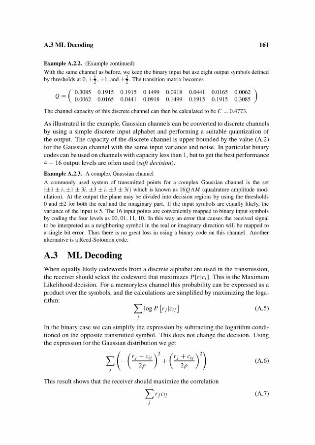
A.3 ML Decoding 161
Example A.2.2. (Example continued)
With the same channel as before, we keep the binary input but use eight output symbols definedby thresholds at 0,± 1
2 ,±1, and ± 32 . The transition matrix becomes
Q =(
0.3085 0.1915 0.1915 0.1499 0.0918 0.0441 0.0165 0.00620.0062 0.0165 0.0441 0.0918 0.1499 0.1915 0.1915 0.3085
)
The channel capacity of this discrete channel can then be calculated to be C = 0.4773.
As illustrated in the example, Gaussian channels can be converted to discrete channelsby using a simple discrete input alphabet and performing a suitable quantization ofthe output. The capacity of the discrete channel is upper bounded by the value (A.2)for the Gaussian channel with the same input variance and noise. In particular binarycodes can be used on channels with capacity less than 1, but to get the best performance4 − 16 output levels are often used (soft decision).
Example A.2.3. A complex Gaussian channel
A commonly used system of transmitted points for a complex Gaussian channel is the set{±1 ± i,±1 ± 3i, ±3 ± i,±3 ± 3i} which is known as 16Q AM (quadrature amplitude mod-ulation). At the output the plane may be divided into decision regions by using the thresholds0 and ±2 for both the real and the imaginary part. If the input symbols are equally likely, thevariance of the input is 5. The 16 input points are conveniently mapped to binary input symbolsby coding the four levels as 00, 01, 11, 10. In this way an error that causes the received signalto be interpreted as a neighboring symbol in the real or imaginary direction will be mapped toa single bit error. Thus there is no great loss in using a binary code on this channel. Anotheralternative is a Reed-Solomon code.
A.3 ML DecodingWhen equally likely codewords from a discrete alphabet are used in the transmission,the receiver should select the codeword that maximizes P[r |ci ]. This is the MaximumLikelihood decision. For a memoryless channel this probability can be expressed as aproduct over the symbols, and the calculations are simplified by maximizing the loga-rithm: ∑
j
log P[r j |ci j
](A.5)
In the binary case we can simplify the expression by subtracting the logarithm condi-tioned on the opposite transmitted symbol. This does not change the decision. Usingthe expression for the Gaussian distribution we get
∑j
(−(
r j − ci j
2ρ
)2
+(
r j + ci j
2ρ
)2)
(A.6)
This result shows that the receiver should maximize the correlation∑
j
r j ci j (A.7)

162 Communication channels
or equivalently minimize the error
∑j
ci j(ci j − r j
)(A.8)
Thus when the channel output is quantized using A − 1 equally spaced thresholds, wecan simply use the integers {0, 1, . . . , A − 1} as weights for the symbols.
Using such a set of weight, the Viterbi algorithm for convolutional codes, iterative de-coding of block codes and certain other techniques can be modified with these so-calledsoft decisions.
Appendix B
Solutions to selected problems
B.1 Solutions to problems in Chapter 1Problem 1.5.1
1) No, the sum of the last two words is not in there. Or 5 is not a power or of 2.
2) If we add (010110), (011001) and (100101) we get a linear code.
3) There are many possibilities, e.g. (101010), (010110), (001111).
Problem 1.5.2
1) Using row operations we get
G =
1 0 0 1 0 10 1 0 1 1 00 0 1 1 1 1
2) Since HC⊥ = GC this is the G that we have.
3) No, G(111111)T = (100) �= (000).
Problem 1.5.3
1) The dimension of the code is 4 and therefore the dimension of the dual is 12−4 = 8.
To get the minimum distance of the code (= minimum weight) at this point we listthe 24 = 16 codewords and find dmin = 6.
For the dual code we have HC⊥ = GC and since columns 1, 4 and 5 in G sum tozero and there is no zero column and no two equal columns, the minimum distanceof C⊥ is 3.
2) The original code can correct two errors and the dual code can correct one error.
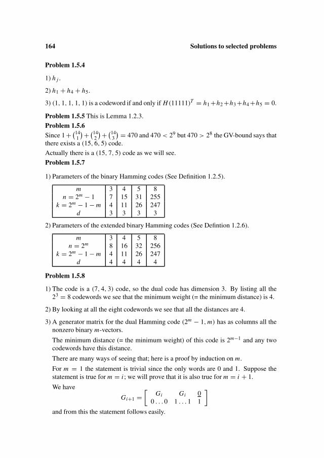
164 Solutions to selected problems
Problem 1.5.4
1) h j .
2) h1 + h4 + h5.
3) (1, 1, 1, 1, 1) is a codeword if and only if H (11111)T = h1 +h2 +h3 +h4 +h5 = 0.
Problem 1.5.5 This is Lemma 1.2.3.
Problem 1.5.6Since 1 + (14
1
)+ (142
)+ (143
) = 470 and 470 < 29 but 470 > 28 the GV-bound says thatthere exists a (15, 6, 5) code.
Actually there is a (15, 7, 5) code as we will see.
Problem 1.5.7
1) Parameters of the binary Hamming codes (See Definition 1.2.5).
m 3 4 5 8n = 2m − 1 7 15 31 255
k = 2m − 1 − m 4 11 26 247d 3 3 3 3
2) Parameters of the extended binary Hamming codes (See Defintion 1.2.6).
m 3 4 5 8n = 2m 8 16 32 256
k = 2m − 1 − m 4 11 26 247d 4 4 4 4
Problem 1.5.8
1) The code is a (7, 4, 3) code, so the dual code has dimension 3. By listing all the23 = 8 codewords we see that the minimum weight (= the minimum distance) is 4.
2) By looking at all the eight codewords we see that all the distances are 4.
3) A generator matrix for the dual Hamming code (2m − 1, m) has as columns all thenonzero binary m-vectors.
The minimum distance (= the minimum weight) of this code is 2m−1 and any twocodewords have this distance.
There are many ways of seeing that; here is a proof by induction on m.
For m = 1 the statement is trivial since the only words are 0 and 1. Suppose thestatement is true for m = i ; we will prove that it is also true for m = i + 1.
We have
Gi+1 =[
Gi Gi 00 . . . 0 1 . . . 1 1
]
and from this the statement follows easily.

B.1 Solutions to problems in Chapter 1 165
Problem 1.5.9
1) B(2) has generator matrix
G =
1 0 1 00 1 1 01 1 1 0
From this the result is trivial.
2) This follows directly from Problem 1.5.8.
3) Since the distance between any two words is n2 this is obvious (except that the all 1s
word and the all −1s word are not orthogonal.
Problem 1.5.10
1) We get
n∗ = n − 1
k∗ = k (since d ≥ 2)
d∗ ={
d if d is even
d − 1 if d is odd
d is even if all minimum weight words have a zero in the deleted position.
2) We get
n∗ = n − 1
k∗ = k − 1
d∗ = d
Problem 1.5.11
We get
kext = k and dext,min ={
d if d is even
d + 1 otherwise
The parity check matrix for the extended code is obtained by adding a column of zeroesto H and the a row of 1s, i.e.
Hext =
Hc 0...
01 . . . 1
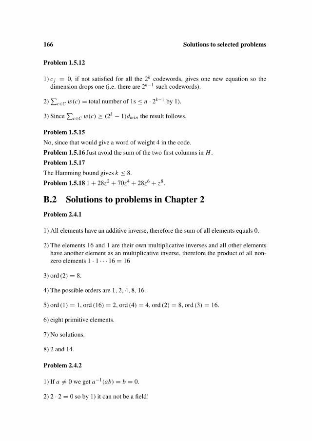
166 Solutions to selected problems
Problem 1.5.12
1) c j = 0, if not satisfied for all the 2k codewords, gives one new equation so thedimension drops one (i.e. there are 2k−1 such codewords).
2)∑
c∈C w(c) = total number of 1s ≤ n · 2k−1 by 1).
3) Since∑
c∈C w(c) ≥ (2k − 1)dmin the result follows.
Problem 1.5.15
No, since that would give a word of weight 4 in the code.
Problem 1.5.16 Just avoid the sum of the two first columns in H .
Problem 1.5.17
The Hamming bound gives k ≤ 8.
Problem 1.5.18 1 + 28z2 + 70z4 + 28z6 + z8.
B.2 Solutions to problems in Chapter 2
Problem 2.4.1
1) All elements have an additive inverse, therefore the sum of all elements equals 0.
2) The elements 16 and 1 are their own multiplicative inverses and all other elementshave another element as an multiplicative inverse, therefore the product of all non-zero elements 1 · 1 · · · 16 = 16
3) ord (2) = 8.
4) The possible orders are 1, 2, 4, 8, 16.
5) ord (1) = 1, ord (16) = 2, ord (4) = 4, ord (2) = 8, ord (3) = 16.
6) eight primitive elements.
7) No solutions.
8) 2 and 14.
Problem 2.4.2
1) If a �= 0 we get a−1(ab) = b = 0.
2) 2 · 2 = 0 so by 1) it can not be a field!
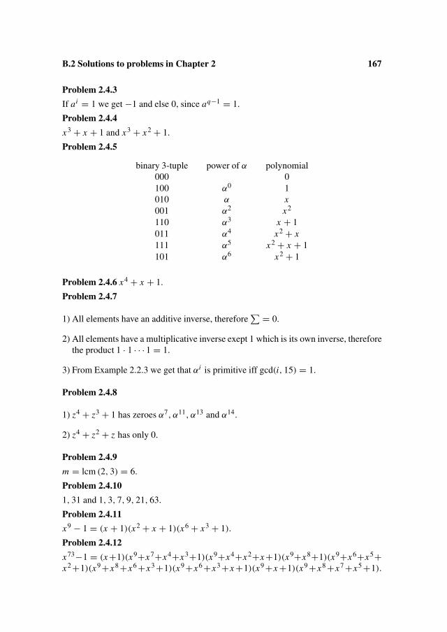
B.2 Solutions to problems in Chapter 2 167
Problem 2.4.3
If ai = 1 we get −1 and else 0, since aq−1 = 1.
Problem 2.4.4
x3 + x + 1 and x3 + x2 + 1.
Problem 2.4.5
binary 3-tuple power of α polynomial000 0100 α0 1010 α x001 α2 x2
110 α3 x + 1011 α4 x2 + x111 α5 x2 + x + 1101 α6 x2 + 1
Problem 2.4.6 x4 + x + 1.
Problem 2.4.7
1) All elements have an additive inverse, therefore∑ = 0.
2) All elements have a multiplicative inverse exept 1 which is its own inverse, thereforethe product 1 · 1 · · · 1 = 1.
3) From Example 2.2.3 we get that αi is primitive iff gcd(i, 15) = 1.
Problem 2.4.8
1) z4 + z3 + 1 has zeroes α7, α11, α13 and α14.
2) z4 + z2 + z has only 0.
Problem 2.4.9
m = lcm (2, 3) = 6.
Problem 2.4.10
1, 31 and 1, 3, 7, 9, 21, 63.
Problem 2.4.11
x9 − 1 = (x + 1)(x2 + x + 1)(x6 + x3 + 1).
Problem 2.4.12
x73−1 = (x +1)(x9+x7+x4+x3+1)(x9+x4+x2+x +1)(x9+x8+1)(x9+x6+x5+x2 +1)(x9+x8 +x6 +x3 +1)(x9+x6 +x3 +x +1)(x9+x +1)(x9 +x8 +x7 +x5 +1).

168 Solutions to selected problems
Problem 2.4.13 x85 −1 = (x +1)(x8 + x6 + x5 + x4 + x2 + x +1)(x8 + x7 + x5 + x4 +x3 + x2 +1)(x8 + x7 + x6 + x4 + x2 + x +1)(x8+ x7 + x3 + x +1)(x8+ x5 + x4 + x3 +x2 + x + 1)(x8 + x7 + x6 + x5 + x4 + x3 + 1)(x8 + x5 + x4 + x3 + 1)(x4 + x3 + x2 +x +1)(x8 + x7 + x6 + x4 + x3 + x2 +1)(x9 + x7 + x5 + x2 +1)(x9 + x6 + x3 + x +1).
Problem 2.4.14 x18 − 1 = (x9 − 1)2.
Problem 2.4.15 Yes it is on the list, see Appendix C, m = 8, i = 5.
Problem 2.4.16
3) x + 1.
4) x, x2, x4, x8.
B.3 Solutions to problems in Chapter 3Problem 3.4.1
1) µ = np = 16 · 0.01 = 0.16 and σ = √np(1 − p) = 0.401
2) From (3.2) we get 0.852, 0.138, 0.010, 0.0005, 0.00002.
3) From (3.3) we get 0.852, 0.134, 0.011, 0.00058, 0.00002. Thus the agreement isquite good for these parameters.
4) From (3.4) we get Pfail = 1 − 0.852 − 0.138 = 0.011 since t = 1 here.
5) So it is the probability of getting three errors i.e. 0.0005.
Problem 3.4.2
1) The weight distribution shows d = 5, thus t = 2.
2) Pfail = P(> 2) = 0.0004.
3) 3 bit errors cause a decoding error if the received vector is at distance 2 from acodeword of weight 5. Thus there are 18·(53
) = 180 such error patterns (exact result).
The total number of weight 3 words is(15
3
) = 455. The number could also be foundusing (3.6) with j = 3, w = 5, s = 2, i = 0.
4) Perr = 180 ·0.013 ·0.9912 = 0.00016. The next term for j = 4 gives 90+450 errorpatterns, but the total probability is much smaller.
Problem 3.4.3
1) The minimum distance is 6, so the code corrects two errors.
2) Assuming that only two errors are corrected we havePf ail ≈ P(3) = (16
3
) · p3 · (1 − p)13 = 0.0005.
3) From (3.5) we get T (4, 2, 6) = 15 and T (6, 2, 6) = 6 · 10 = 60.

B.4 Solutions to problems in Chapter 4 169
Problem 3.4.4
1) np = 2.56
2) P(9) = 0.00094 , P(10) = 0.00024 , P(11) = 0.00005 so P(> 8) = 0.00125.
3) We get about 0.00132, all terms are slightly larger.
B.4 Solutions to problems in Chapter 4
Problem 4.3.1
1) The entropy of the source is H = 1.5 bits.
2) Hmax = log(3) = 1.585 bits.
3) C = {0, 10, 11}.
4)[
12 , 1
4 , 14
]for [0, 1,−1]. V is not memoryless. There is a one-to-one mapping be-
tween the binary and the ternary sequences.
Problem 4.3.2
1) When the input distribution is(
12 , 1
2
), the output distribution becomes P(Y ) =[
516 , 3
16 , 316 , 5
16
].
2) I = H (Y ) − H( Y
X
) = 1 + H(
38
)− 7
4 = 0.204 bits.
3) C = I ; this is the maximizing distribution .
Problem 4.3.3
1) C = 1 − H (0.05) = 0.714 bits.
2) The average number of errors is ta = 256 · 0.05 = 12.8.
3) The Hamming bound gives : log2
((256t
))< 256 − 160 thus t = 19.
4) P(e) = P[> 19 errors] = (25620
)p20(1 − p)236 + (256
21
)p21(1 − p)235 + · · · = 0.03.
5) The Gilbert bound for the same parameters is dg = 21 by a similar calculation.(There is a code with d = 26.)

170 Solutions to selected problems
B.5 Solutions to problems in Chapter 5Problem 5.5.1
1) There are (4, 1, 4), (4, 3, 2) and (4, 4, 1) binary codes.
2) A (4, 2, 3) ternary code could have
H =[
1 0 1 10 1 1 −1
]
Problem 5.5.2
1)
G =
1 1 1 1 1 11 3 2 6 4 51 2 4 1 2 41 6 1 6 1 6
2) Using the polynomials
2(x − 3)(x − 2)(x − 6)
(x − 1)(x − 2)(x − 6)
2(x − 1)(x − 3)(x − 6)
2(x − 1)(x − 3)(x − 2)
we get
G =
1 0 0 0 6 20 1 0 0 6 20 0 1 0 2 10 0 0 1 5 6
3) dmin = n − k + 1 = 6 − 4 + 1 = 3.
4) Addition of the second and fourth row of G from 1) gives (2, 2, 3, 5, 5, 4) so r =(2, 4, 3, 5, 5, 4).
5) l0 = 4 and l1 = 1 so we have seven coeffiencients. (and six equations).
6) Q0(x) = 4x4 + 3x3 + 4x2 + 3x, Q1(x) = x + 4 so − Q0(c)Q1(x)
= x + x3.
7) H =[
1 3 2 6 4 51 2 4 1 2 4
]
8) A single error would give a syndrome that is a column of H .

B.6 Solutions to problems in Chapter 6 171
Problem 5.5.3
1) (1, α, α2, α3, α4, α5, α6) + (1, α2, α4, α6, α, α3, α5) = (0, α5, α, α4, α2, α2, α).
2) (8, 3, 6).
3) With r = (0, α5, α, 0, 0, α2, α) one gets Q0(x) = x4 + α2x3 + α2x2 + x andQ1(x) = x2 + α6x + 1 and f (x) = x + x2.
4)
H =
1 α α2 α3 α4 α5 α6
1 α2 α4 α6 α α3 α5
1 α3 α6 α2 α5 α α4
1 α4 α α5 α2 α6 α3
5) One error would give: S2S1
= S3S2
= S4S3
.
Problem 5.5.4
1) Q1(x) = x2 + α6x + 1 = (x − α3)(x − α4).
2) yes.
3) α4 and α2.
B.6 Solutions to problems in Chapter 6Problem 6.5.1
1) x9 − 1 = (x3 − 1)(x6 + x3 + 1).
2) k = 3.
3)
G =
1 0 0 1 0 0 1 0 00 1 0 0 1 0 0 1 00 0 1 0 0 1 0 0 1
4) Yes, since x8 + x6 + x5 + x3 + x2 + 1 = (x2 + 1)(x6 + x3 + 1).
5) dmin = 3 (List the eight codewords).
Problem 6.5.2
1) k = 15 − 5 = 10.
2) No g(x) does not divide.

172 Solutions to selected problems
3) The possible generator polynomials are
(x3 + 1)(x4 + x + 1)
(x3 + 1)(x4 + x3 + 1)
(x3 + 1)(x4 + x3 + x2 + x + 1)
4) 25 but two of them are trivial so they are 30.
Problem 6.5.3
1) h(x) = x15 − 1
x4 + x + 1= x11 + x8 + x7 + x5 + x3 + x2 + x + 1.
so
H =
1 1 1 1 0 1 0 1 1 0 0 1 0 0 00 1 1 1 1 0 1 0 1 1 0 0 1 0 00 0 1 1 1 1 0 1 0 1 1 0 0 1 00 0 0 1 1 1 1 0 1 0 1 1 0 0 1
2) dmin = 3.
3) C is the (15, 11, 3) Hamming code.
4) The dual code has dimension 4.
Problem 6.5.4
g(x)|c(x) so 0 = c(1) = c0 + c1 + · · · + cn−1 ⇔ c has even weight.
Problem 6.5.5
Since C has a word of odd weight x+1 does not divide g(x) and therefore g(x)∣∣ xn−1
x+1 =1 + x + · · · + xn−1 so (1111 . . .1) is a codeword.
Problem 6.5.6
1) g(x) has among its zeroes β, β2, β3, β4 so dmin ≥ 5.
2) g⊥(x) = (x − 1)mβ(x)mβ7(x)mβ3(x) so,
3) d⊥min ≥ 6.
Problem 6.5.7
g(x) has among its zeroes α−2, α−1, 1, α, α2 so dmin ≥ 6, but by the Hamming boundthere is no (63, 50, 7) code so it is exactly 6.
Problem 6.5.8
With g(x) = mα(x)mα3(x)mα5(x), α primitive in F25 we get a (31, 16, 7) code andthis is best possible.
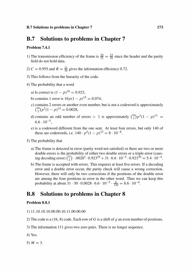
B.7 Solutions to problems in Chapter 7 173
B.7 Solutions to problems in Chapter 7Problem 7.4.1
1) The transmission efficiency of the frame is 3032 = 15
16 since the header and the parityfield do not hold data.
2) C = 0.955 and R = 1116 gives the information efficiency 0.72.
3) This follows from the linearity of the code.
4) The probability that a word
a) Is correct is (1 − p)16 = 0.923,
b) contains 1 error is 16 p(1 − p)15 = 0.074,
c) contains 2 errors or another even number, but is not a codeword is approximately(162
)p2(1 − p)14 = 0.0028,
d) contains an odd number of errors > 1 is approximately(16
3
)p3(1 − p)13 =
6.6 · 10−5,
e) is a codeword different from the one sent. At least four errors, but only 140 ofthese are codewords, i.e. 140 · p4(1 − p)12 = 8 · 10−8.
5) The probability that
a) The frame is detected in error (parity word not satisfied) or there are two or moredouble errors is the probability of either two double errors or a triple error (caus-ing decoding error)
(312
) · .00282 · 0.92329 + 31 · 6.6 · 10−5 · 0.92330 = 5.4 · 10−4.
b) The frame is accepted with errors. This requires at least five errors. If a decodingerror and a double error occur, the parity check will cause a wrong correction.However, there will only be two corrections if the positions of the double errorare among the four positions in error in the other word. Thus we can keep thisprobability at about 31 · 30 · 0.0028 · 6.6 · 10−5 · 6
120 = 8.6 · 10−6.
B.8 Solutions to problems in Chapter 8Problem 8.8.1
1) 11.10.10.10.00.00.10.11.00.00.00
2) The code is a (16, 8) code. Each row of G is a shift of g an even number of positions.
3) The information 111 gives two zero pairs. There is no longer sequence.
4) Yes.
5) M = 3.

174 Solutions to selected problems
6) d is even and at most 6. The information 11101110 gives a codeword of weight 4,so d = 4.
7) For all long codes the minimum distance is 6.
Problem 8.8.2
1) Yes.
2) M = 2.
3) 111.010.011.001.101.110.000.000
Problem 8.8.3
1) As noted in Section 8.3 the sequence h for a code of rate 12 is found by reversing g.
Since g is symmetric here, h = g.
2) The nonzero part of the syndrome for a single error is (1011) for the first position ina pair and (1101) for the second position.
3) Adding the two syndromes from the previous question we find that the error11.00.00. . . . gives the syndrome (0110. . . ).
4) From the previous questions it follows that at least three errors are needed to givethe syndrome. One possibility is 10.11.
Problem 8.8.4
1) The reversed sequence is the same as g.
2) There are two different columns (1101) and (1011).
3) Two errors in a pair 00.11.00. . . . gives the right syndrome.
4) There have to be three errors.
Problem 8.8.5
Code from 8.8.1:
1) All row distances are 6, which is also the free distance.
2) 2.
3) Since g = 11.10.01.11 is a codeword, 11.10.00.00 and 00.00.01.11 have the samesyndrome, and at most one of them can be correctly decoded. The error pattern11.00.00.11 would be decoded as 00.10.01.00

B.9 Solutions to problems in Chapter 9 175
Code from 8.8.2:
1) All row distances are 7, which is also the free distance.
2) 3.
3) 111.100.000.000. . . . would be decoded as 000.001.110.000
Problem 8.8.6
1) Generator of punctured code
11.1.01.1
1.10.0.11
11.1.01.1
2) It is enough to find one row. Multiplying by (1011) gives 11.10.10.10.11.10.11Eliminating the punctured 0s give 111.101.111.110 and memory 3.
Problem 8.8.7
1) All row distances are 6 for the first code and 7 for the second. That is also the freedistance.
2) 2 and 3.
3) Take error patterns that are part of codewords (11.10.00. . . . ) and (111.100.000. . . . )
Problem 8.8.8
G = (1 + D + D3, 1 + D2 + D3)
H = (1 + D2 + D3, 1 + D + D3)
G = (1 + D + D2, 1 + D2, 1 + D)
B.9 Solutions to problems in Chapter 9
Problem 9.3.1
1) 2 , g and the sum of the first 3 rows.
2) 8.
3) 00.01.00.00.10. etc.

176 Solutions to selected problems
4) A next state table indicating the next state for each input symbol.
Present state 000/0 001/1 010/2 011/3 100/4 101/5 110/6 111/7Next state on 0 0 2 4 6 0 2 4 6Next state on 1 1 3 5 7 1 3 5 7
The outputs for the transitions listed above are
Present state 0 1 2 3 4 5 6 7Output on 0 00 10 01 11 11 01 10 00Output on 1 11 01 10 00 00 10 01 11
5) 11.10.01.11, 11.01.11.10.11, 11.10.10.01.01.11, 11.01.00.00.10.11
6) 2x6−x10
1−5x2+2x6 = 2x6 + 10x8 + · · ·7) none of weight 7 (all weights are even) two of weight 6 (found in 5)), ten of weight 8.
8) a and b are decoded since they have weight <d f ree
2 , c and f are not uniquely de-coded since the three 1s are among the first six 1s in g. d is decoded as a doubleerror. e is decoded since it has distance > 3 to all nonzero codewords.
9) Since Z = 0.2 , we get Pe < 1.6 · 10−4.
10) about 0.05.
Problem 9.3.2
1) As in Example 9.1.4 ρ0 = y2ρ3. ρ2 = ρ3. ρ1 = y2+x2ρ3. ρ3 = xy3/(1−xy−xy).And the result ρ0 = xy5/(1 − xy − x3y) which agrees with the example.
2) By long division the first terms are found as ρ0 = xy5+x2y6+x4y6+x3y7+2x5y7+x7y7 + · · · (words of weight > 7). Thus there is one word with four 0s and six 1s.
B.10 Solutions to problems in Chapter 10Problem 10.3.1
1) (49, 16, 9).
2) 3. At least two by Lemma 10.1.1, less than four from the comments in the proof.
3) 49 since there are seven words of weight three in the Hamming code.
4) There are three rows in the parity check matrix of the Hamming code. These arecopied to give parity checks on the seven rows and seven columns, however, the lastthree sets of checks are linear combinations of other rows. Thus we get 33 rows,which is the right number.
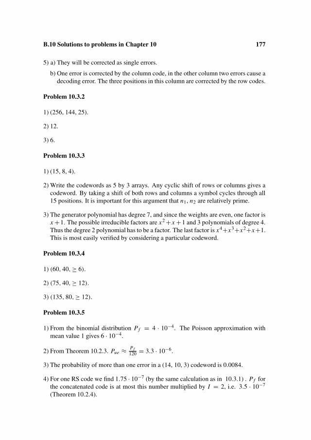
B.10 Solutions to problems in Chapter 10 177
5) a) They will be corrected as single errors.
b) One error is corrected by the column code, in the other column two errors cause adecoding error. The three positions in this column are corrected by the row codes.
Problem 10.3.2
1) (256, 144, 25).
2) 12.
3) 6.
Problem 10.3.3
1) (15, 8, 4).
2) Write the codewords as 5 by 3 arrays. Any cyclic shift of rows or columns gives acodeword. By taking a shift of both rows and columns a symbol cycles through all15 positions. It is important for this argument that n1, n2 are relatively prime.
3) The generator polynomial has degree 7, and since the weights are even, one factor isx +1. The possible irreducible factors are x2 + x +1 and 3 polynomials of degree 4.Thus the degree 2 polynomial has to be a factor. The last factor is x4+x3+x2+x+1.This is most easily verified by considering a particular codeword.
Problem 10.3.4
1) (60, 40,≥ 6).
2) (75, 40,≥ 12).
3) (135, 80,≥ 12).
Problem 10.3.5
1) From the binomial distribution Pf = 4 · 10−4. The Poisson approximation withmean value 1 gives 6 · 10−4.
2) From Theorem 10.2.3. Pue ≈ Pf120 = 3.3 · 10−6.
3) The probability of more than one error in a (14, 10, 3) codeword is 0.0084.
4) For one RS code we find 1.75 · 10−7 (by the same calculation as in 10.3.1) . Pf forthe concatenated code is at most this number multiplied by I = 2, i.e. 3.5 · 10−7
(Theorem 10.2.4).

178 Solutions to selected problems
B.11 Solutions to problems in Chapter 11Problem 11.3.1
1) r(x) = αx + α2x2 + x3, so we know already that the error locations are α, α2, α3
with the corresponding error values α, α2, 1
S1 = r(α) = α2 + α4 + α3 = α12
S2 = r(α2) = α3 + α6 + α6 = α3
S3 = r(α3) = α4 + α8 + α9 = α6
S4 = r(α4) = α5 + α10 + α12 = α11
S5 = r(α5) = α6 + α12 + 1 = α
S6 = r(α6) = α7 + α14 + α3 = α9
SoS(x) = α12x5 + α3x4 + α6x3 + α11x2 + αx + α9.
The Euclidian algorithm on x6 an S(x) gives:
i gi ri qi
−1 0 x6 –
0 1 S(x) –
1 α3x + α9 α8x4 +α3x3 +α8x2 +α3x +α3 α3x + α9
2 α7x2 + α2x + α10 α9x3 +α5x2 +α4 α4x + α11
3 α6x3 + α2x2 + α4x + α12 α13x2 + α6 α14x + α13
so the error locator is g3(x) = α6x3 +α2x3 +α4x +α12 which indeed has α, α2 andα3 as zeroes. Since g′
3 = α6x2 + α4, formula (11.5) gives e1 = α−7 · α15+α6
α8+α4 = α,
e2 = α−14 · α17+α6
α10+α4 = α2, e3 = α−21 · α19+α6
α12+α4 = 1.
2) r(x) = α2x3 + α7x2 + α11x + α6.
S1 = r(α) = α5 + α9 + α12 + α6 = α12
S2 = r(α2) = α8 + α11 + α13 + α6 = α9
S3 = r(α3) = α11 + α13 + α14 + α6 = α5
S4 = r(α4) = α14 + 1 + 1 + α6 = α8
S5 = r(α5) = α2 + α2 + α + α6 = α11
S6 = r(α6) = α5 + α4 + α2 + α6 = α13
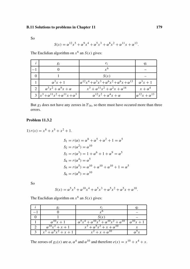
B.11 Solutions to problems in Chapter 11 179
So
S(x) = α12x5 + α9x4 + α5x3 + α8x2 + α11x + α13.
The Euclidian algorithm on x6 an S(x) gives:
i gi ri qi
−1 0 x6 –
0 1 S(x) –
1 α3x + 1 α12x4 +α3x3 +α6x2 +α6x +α13 α3x + 1
2 α3x2 + α9x + α x3 + α11x2 + α2x + α14 x + α4
3 x3 +α11x2 +α11x +α3 α12x2 + α4x + α α12x + α13
But g3 does not have any zeroes in F16, so there must have occured more than threeerrors.
Problem 11.3.2
1) r(x) = x8 + x5 + x2 + 1.
S1 = r(α) = α8 + α5 + α2 + 1 = α5
S2 = r(α2) = α10
S3 = r(α3) = 1 + α6 + 1 + α9 = α5
S4 = r(α4) = α5
S5 = r(α5) = α10 + α10 + α10 + 1 = α5
S6 = r(α6) = α10
So
S(x) = α5x5 + α10x4 + α5x3 + α5x2 + α5x + α10.
The Euclidian algorithm on x6 an S(x) gives:
i gi ri qi
−1 0 x6 –0 1 S(x) –1 α10x + 1 α5x4 + α10x3 + α10x2 + α10 α10x + 12 α10x2 + x + 1 x3 + α5x2 + x + α10 x3 x3 + α5x2 + x + 1 x2 + x + α10 α5x
The zeroes of g3(x) are α, α4 and α10 and therefore e(x) = x10 + x4 + x .

180 Solutions to selected problems
2) r(x) = x11 + x7 + x3 + x2 + x + 1.
S1 = r(α) = α11 + α7 + α3 + α2 + α + 1 = α9
S2 = r(α2) = α3
S3 = r(α3) = α3 + α6 + α9 + α6 + α3 + 1 = α7
S4 = r(α4) = α6
S5 = r(α5) = α10 + α5 + 1 + α10 + α5 + 1 = 0
S6 = r(α6) = α14
SoS(x) = α9x5 + α3x4 + α7x3 + α6x2 + α14.
The Euclidian algorithm on x6 an S(x) gives:
i gi ri qi
−1 0 x6 –0 1 S(x) –1 α6x + 1 α8x4 + α2x3 + α6x2 + α5x + α14 α6x + 12 α7x2 + αx + 1 x + α14 αx
Here g2(x) has α10 and α13 as zeroes, so e(x) = x10 + x13 and we decode intox13 + x11 + x10 + x7 + x3 + x2 + x + 1.
B.12 Solutions to problems in Chapter 12Problem 12.4.1
n = 31, k = 10 so dmin = 22.
1) With list size 2, we get τ < 31 · 23 − 2
2 · 9 = 20 23 − 9, so τ ≤ 11.
2) With list size 3, we get τ < 31 · 34 − 3
2 · 9 = 394 , so the answer is τ ≤ 11!
Problem 12.4.2
• n = 31, k = 10.
l = 1 gives τ ≤ 13.
l = 2 gives τ ≤ 16.
l = 3 gives τ ≤ 18.
l = 4 gives τ ≤ 16.
so the optimal list size is 3.
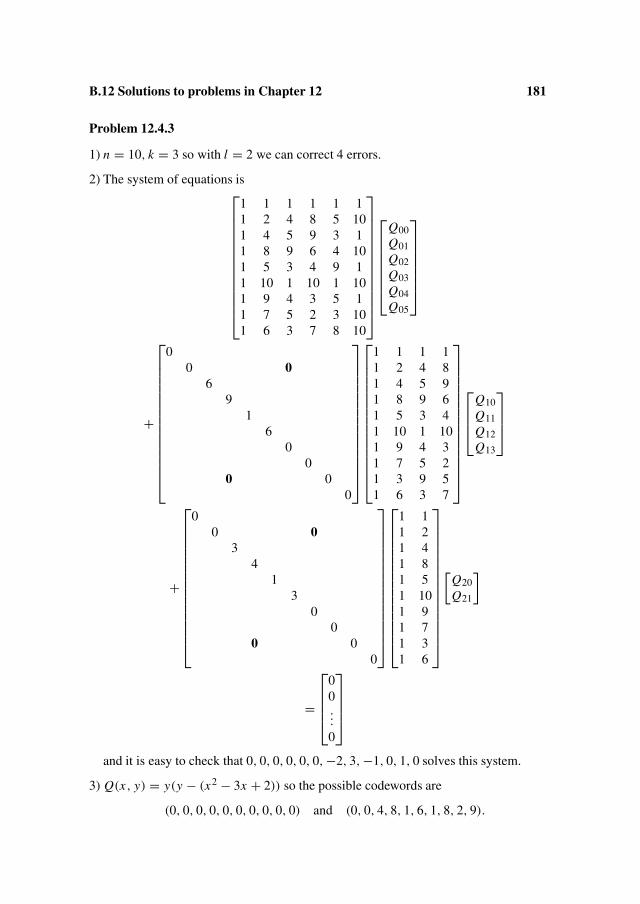
B.12 Solutions to problems in Chapter 12 181
Problem 12.4.3
1) n = 10, k = 3 so with l = 2 we can correct 4 errors.
2) The system of equations is
1 1 1 1 1 11 2 4 8 5 101 4 5 9 3 11 8 9 6 4 101 5 3 4 9 11 10 1 10 1 101 9 4 3 5 11 7 5 2 3 101 6 3 7 8 10
Q00Q01Q02Q03Q04Q05
+
00 0
69
16
00
0 00
1 1 1 11 2 4 81 4 5 91 8 9 61 5 3 41 10 1 101 9 4 31 7 5 21 3 9 51 6 3 7
Q10Q11Q12Q13
+
00 0
34
13
00
0 00
1 11 21 41 81 51 101 91 71 31 6
[Q20Q21
]
=
00...
0
and it is easy to check that 0, 0, 0, 0, 0, 0,−2, 3,−1, 0, 1, 0 solves this system.
3) Q(x, y) = y(y − (x2 − 3x + 2)) so the possible codewords are
(0, 0, 0, 0, 0, 0, 0, 0, 0, 0) and (0, 0, 4, 8, 1, 6, 1, 8, 2, 9).

182 Solutions to selected problems
B.13 Solutions to problems in Chapter 13Problem 13.5.1 The parity bits are (00011001001).
The encoding can be interpreted as correcting erasures on the last n − k positions.
The decoded word is (110110110110110110110)
Problem 13.5.2The code has n = 12 symbols and 8 parity checks, 7 of these independent. So it is a(12, 5, 4) code.
1 1 1 0 0 0 0 0 0 0 0 01 0 0 1 1 0 0 0 0 0 0 00 1 0 0 0 1 1 0 0 0 0 00 0 1 0 0 0 0 1 1 0 0 00 0 0 1 0 0 0 1 0 1 0 00 0 0 0 1 0 1 0 0 0 1 00 0 0 0 0 1 0 0 1 0 0 10 0 0 0 0 0 0 0 0 1 1 1
A tree code can have four parity checks and nine symbols. A single error is identifiedby the two parity checks that fail. They can be in the same tree code, or there may beone in each code.
Problem 13.5.3Three errors are corrected, but the result depends on the order in which the positionsare considered.
With message passing the weights indicate that three errors have occurred, but there isnot a unique result.
B.14 Solutions to problems in Chapter 14Problem 14.3.1
1) (64, 22,≥ 37).
2) Let α be a primitive element of F16 with α4 + α + 1 = 0, then the 64 points on thecurve x5 + y4 + y = 0 are
(0, 0), (0, 1), (0, α5), (0, α10);(1, α), (α3, α), (α6, α), (α12, α), (α9, α);
(1, α2), (α3, α2), (α6, α2), (α12, α2), (α9, α2);(1, α4), (α3, α4), (α6, α4), (α12, α4), (α9, α4);(1, α8), (α3, α8), (α6, α8), (α12, α8), (α9, α8);(α, α6), (α4, α6), (α7, α6), (α10, α6), (α13, α6);(α, α7), (α4, α7), (α7, α7), (α10, α7), (α13, α7);

B.14 Solutions to problems in Chapter 14 183
(α, α9), (α4, α9), (α7, α9), (α10, α9), (α13, α9);(α, α13), (α4, α13), (α7, α13), (α10, α13), (α13, α13);
(α2, α3), (α5, α3), (α8, α3), (α11, α3), (α14, α3);(α2, α11), (α5, α11), (α8, α11), (α11, α11), (α14, α11);(α2, α12), (α5, α12), (α8, α12), (α11, α12), (α14, α12);(α2, α14), (α5, α14), (α8, α14), (α11, α14), (α14, α14)
and the 22 polynomials in which one evaluates these points are:
1, x, y, x2, xy, y2, x3, x2y, xy2, y3, x4, x3 y,
x2y2, xy3, y4, x4 y, x3y2, x2y3, xy4, y5, x4y, x3y3.
This gives a 22 × 64 generator matrix for the code.
3) (64, 42,≥ 17).
4) Since H (22)⊥ = H (42) we can copy the previous method.
Problem 14.3.3
xq+1 − yq − y = (a(x) + yb(x, y))(c(x) + yd(x, y))
= a(x)c(x) + y(b(x, y)c(x) + d(x, y)a(x)) + y2b(x, y)d(x, y)
and therefore a(x)c(x) = xq+1 so a(x) = xq+1−i ,c(x) = xi but this implies
b(x, y)xi + d(x, y)xq+1−i + yb(x, y)d(x, y) = −yq−1 − 1
and hence i = 0 and b(x, y) = −1 or i = q + 1 and d(x, y) = −1. In the first casewe get d(x, y) = yq−2 and in the second case b(x, y) = yq−1. If we insert these inthe original expression we get a contradiction.
Problem 14.3.4The zeroes of xq + x in Fq2 for q even are 0 and αi(q+1), i = 0, 1, . . . , q − 2 where α
is a primitive element of Fq2 and for q odd the zeroes are
0 and αq+1
2 · j , j = 1, 3, . . . , 2(q − 1) − 1, where α is a primitive lement of Fq2 .
Problem 14.3.5If α(q−1)(a1+a2) = 1 we have q2 − 1
∣∣(q − 1)(a1 + a2) and hence a1 + a2 = h(q + 1)
with h ≥ 1. So the relevant sum in this case is
q−2∑i=0
∑−βq + β = αi(q+1)βb1+b2
q∑j=0
α2ih(q+1)
= −∑
βb1+b2(βq + β
)2h
=∑
βb1+b2
2h∑l=0
(2h
l
)βlq − β2h−l = 0

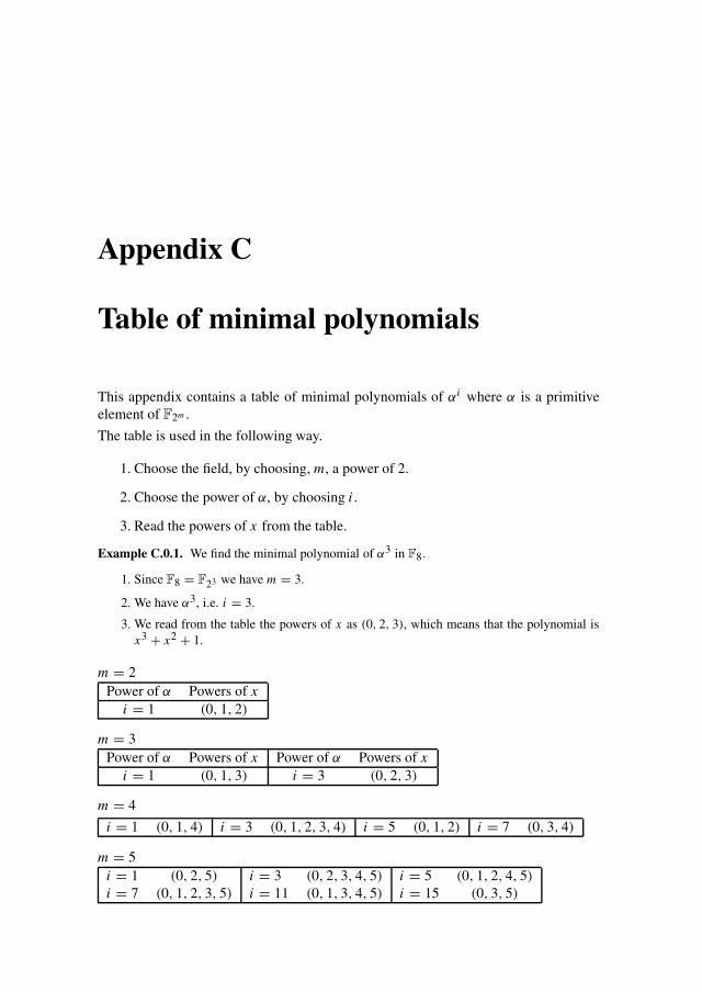
Appendix C
Table of minimal polynomials
This appendix contains a table of minimal polynomials of αi where α is a primitiveelement of F2m .
The table is used in the following way.
1. Choose the field, by choosing, m, a power of 2.
2. Choose the power of α, by choosing i .
3. Read the powers of x from the table.
Example C.0.1. We find the minimal polynomial of α3 in F8.
1. Since F8 = F23 we have m = 3.
2. We have α3, i.e. i = 3.
3. We read from the table the powers of x as (0, 2, 3), which means that the polynomial isx3 + x2 + 1.
m = 2Power of α Powers of x
i = 1 (0, 1, 2)
m = 3Power of α Powers of x Power of α Powers of x
i = 1 (0, 1, 3) i = 3 (0, 2, 3)
m = 4
i = 1 (0, 1, 4) i = 3 (0, 1, 2, 3, 4) i = 5 (0, 1, 2) i = 7 (0, 3, 4)
m = 5i = 1 (0, 2, 5) i = 3 (0, 2, 3, 4, 5) i = 5 (0, 1, 2, 4, 5)
i = 7 (0, 1, 2, 3, 5) i = 11 (0, 1, 3, 4, 5) i = 15 (0, 3, 5)
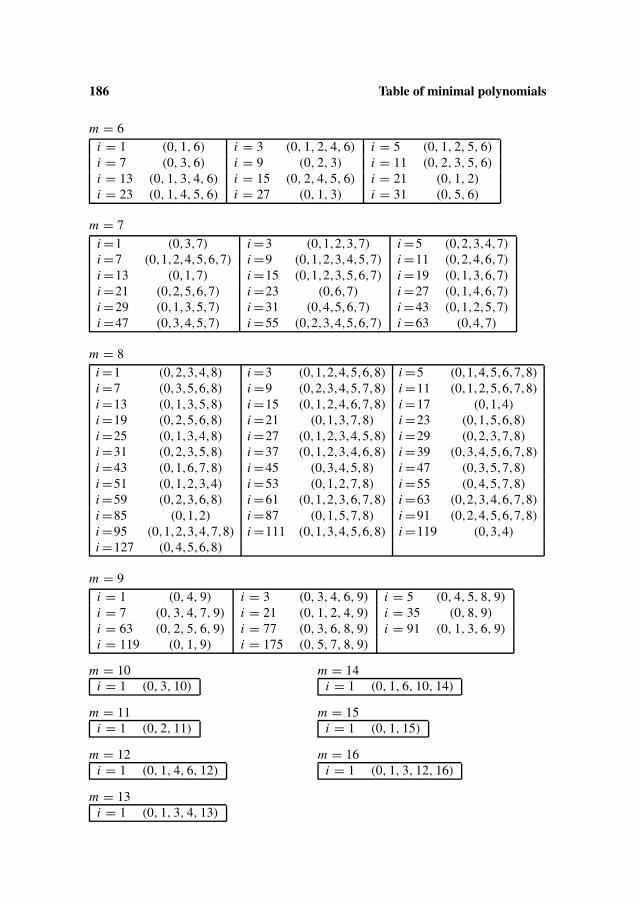
186 Table of minimal polynomials
m = 6i = 1 (0, 1, 6) i = 3 (0, 1, 2, 4, 6) i = 5 (0, 1, 2, 5, 6)
i = 7 (0, 3, 6) i = 9 (0, 2, 3) i = 11 (0, 2, 3, 5, 6)
i = 13 (0, 1, 3, 4, 6) i = 15 (0, 2, 4, 5, 6) i = 21 (0, 1, 2)
i = 23 (0, 1, 4, 5, 6) i = 27 (0, 1, 3) i = 31 (0, 5, 6)
m = 7i =1 (0,3,7) i =3 (0,1,2,3,7) i =5 (0,2,3,4,7)
i =7 (0,1,2,4,5,6,7) i =9 (0,1,2,3,4,5,7) i =11 (0,2,4,6,7)
i =13 (0,1,7) i =15 (0,1,2,3,5,6,7) i =19 (0,1,3,6,7)
i =21 (0,2,5,6,7) i =23 (0,6,7) i =27 (0,1,4,6,7)
i =29 (0,1,3,5,7) i =31 (0,4,5,6,7) i =43 (0,1,2,5,7)
i =47 (0,3,4,5,7) i =55 (0,2,3,4,5,6,7) i =63 (0,4,7)
m = 8i =1 (0,2,3,4,8) i =3 (0,1,2,4,5,6,8) i =5 (0,1,4,5,6,7,8)
i =7 (0,3,5,6,8) i =9 (0,2,3,4,5,7,8) i =11 (0,1,2,5,6,7,8)
i =13 (0,1,3,5,8) i =15 (0,1,2,4,6,7,8) i =17 (0,1,4)
i =19 (0,2,5,6,8) i =21 (0,1,3,7,8) i =23 (0,1,5,6,8)
i =25 (0,1,3,4,8) i =27 (0,1,2,3,4,5,8) i =29 (0,2,3,7,8)
i =31 (0,2,3,5,8) i =37 (0,1,2,3,4,6,8) i =39 (0,3,4,5,6,7,8)
i =43 (0,1,6,7,8) i =45 (0,3,4,5,8) i =47 (0,3,5,7,8)
i =51 (0,1,2,3,4) i =53 (0,1,2,7,8) i =55 (0,4,5,7,8)
i =59 (0,2,3,6,8) i =61 (0,1,2,3,6,7,8) i =63 (0,2,3,4,6,7,8)
i =85 (0,1,2) i =87 (0,1,5,7,8) i =91 (0,2,4,5,6,7,8)
i =95 (0,1,2,3,4,7,8) i =111 (0,1,3,4,5,6,8) i =119 (0,3,4)
i =127 (0,4,5,6,8)
m = 9i = 1 (0, 4, 9) i = 3 (0, 3, 4, 6, 9) i = 5 (0, 4, 5, 8, 9)
i = 7 (0, 3, 4, 7, 9) i = 21 (0, 1, 2, 4, 9) i = 35 (0, 8, 9)
i = 63 (0, 2, 5, 6, 9) i = 77 (0, 3, 6, 8, 9) i = 91 (0, 1, 3, 6, 9)
i = 119 (0, 1, 9) i = 175 (0, 5, 7, 8, 9)
m = 10 m = 14i = 1 (0, 3, 10) i = 1 (0, 1, 6, 10, 14)
m = 11 m = 15i = 1 (0, 2, 11) i = 1 (0, 1, 15)
m = 12 m = 16i = 1 (0, 1, 4, 6, 12) i = 1 (0, 1, 3, 12, 16)
m = 13i = 1 (0, 1, 3, 4, 13)
Bibliography
Readers looking for additional information can use the following directions and start-ing points.
TextbooksThe following two textbooks give an introduction to codes with some emphasis onapplications in communication systems
Shu Lin and Daniel J. Costello, Jr. Error Control Coding: Fundamentals andApplications. Prentice-Hall, Englewood Cliffs, NJ, USA, 1983, 2nd ed. 2004.ISBN 0-13-283796-X.
R. Blahut. Algebraic Codes for Data Transmission. Cambridge UniversityPress, 2003.
An introduction to convolutional codes with in- depth treatment of linear encoders maybe found in
Rolf Johannesson and Kamil Sh. Zigangirov. Fundamentals of ConvolutionalCoding. IEEE Press, New York, NY, USA, 1999. ISBN 0-7803-3483-3.
Reference booksConstructions and combinatorial properties of error-correcting codes are treated ingreat detail in
F. J. MacWilliams and N. J. A. Sloane. The Theory of Error-Correcting Codes,volume 16 of North-Holland Mathematical Library. North-Holland, 1983,reprinted 1998.
An extensive set of reference articles, somewhat uneven in the treatment of the differentproblems.
V. S. Pless and W. Huffman, editors. Handbook of Coding Theory. Elsevier,1999.
188 Table of minimal polynomials
The following classical textbook is still a valuable reference on cyclic codes.
W. W. Peterson and E. J. Weldon. Error Correcting Codes. John Wiley & SonsPublishers, (New York NY),
Professional journalsThe most important journal covering original research on coding theory.
IEEE Transactions on Information Theory.
The following special issue is particularly important as an entry point into the literature
Information Theory 1948-98 Special Commemorative Issue. IEEE Transactionson Information Theory, 44(6), October 1998.
This issue contains a number of surveys with extensive lists of references.
Developing areas and applications are often treated in special issues of this and otherjournals. Some recent issues are
Special issue on graphs and iterative algorithms. IEEE Transactions on Infor-mation Theory, February 2001.
Signal Processing for High-Density Storage Channels. IEEE Journal on SelectedAreas in Communications, April 2001.
Important mathematics journals are
• North Holland. Discrete Mathematics.
• Academic Press. Finite Fields and their Applications.
• Kluwer Acad. Publ. Designs, Codes and Cryptograpy.
• Springer. Applicable Algebra in Engineering, Communication and Computing.
Applications standardsThe details of codes used in particular systems may be found in documents publishedby various standards organizations. However, the information will often have to beextracted from large amounts of related information.
The Consultative Committee for Space Data Systems is an international body that setscommon standards for the major space agencies. The documents are available at
www.ccsds.org
Standards for commercial communication systems including mobile communicationmay be obtained from European Telecommunication Standards Institute at
www.etsi.org

189
ImplementationsDetails of coding and decoding algorithms are covered in some of the books and jour-nals mentioned above. However, practical decoders often use special circuits, and manyare based on programmable logic arrays. Some information may be obtained from ma-jor suppliers of such circuits at
www.xilinx.com or www.altera.com
Tables of codesSome reseachers maintain web sites which are updated with information about the bestknown codes etc. A useful site is
www.win.tue.nl/∼aeb/voorlincod.htmlwhich give parameters of best known codes.
Internet resourcesMuch information can be obtained by using standard search engines as Google.com.The entry Reed-Solomon codes gives many useful references. However it should benoted that the information cannot always be expected to be correct or up-to-date. Moreinformation about coding in space system can be found at
www331.jpl.nasa.gov/public/JPLtcodes.html
Finally the authors plan to make sample problem sheets in maple r© and Matlab r© aswell as corrections to this book available on
www.mat.dtu.dk/publications/books


Index
A, 11A(z), 11Aw , 11algebraic geometry codes, 151α, 20
B, 11B(z), 11B f , 74Bw, 11basis, 2BCH-bound, 66BCH-codes, 69BEC, 44β, 27binary, 1
channel, 74code, 1erasure channel, 44field, 1Hamming code, 7symmetric channel, 34, 43
binomial distribution, 33biorthogonal code, 7bit-flipping, 139block codes, 1body, 74bounded distance decoding, 34BSC, 34, 43
C(Y | X), 43C⊥, 4Cs , 68Cs(sub), 68C, 1c, 4capacity of a discrete channel, 43catastrophic error-propagation, 85catastropic encoding, 85
chain of state transitions, 99channel symbols, 73circuit, 99circulant matrix, 86code
algebraic geometry, 151binary, 1biorthogonal, 7block, 1column tree, 144composite, 109concatenated, 113convolutional, 83cyclic, 63dual regular convolution, 89Golay, 71Hamming, 7Hermitian, 152length, 1low-density parity check, 137polynomial, 63product, 109punctured, 90punctured dual, 91quasi-cyclic, 86Reed-Solomon, 50regular unit memory, 93row tree, 144shortened, 90tail-biting, 86tree, 140unit memory, 93
codeword, 1number of ∼s, 2
column error probability, 115column tree code, 144composite code, 109concatenated code, 80, 112, 113
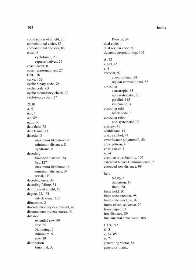
192 Index
construction of a field, 23convolutional codes, 83convolutional encoder, 88coset, 8
cyclotomic, 27representatives, 27
coset leader, 8coset representatives, 27CRC, 76curve, 152cyclic binary code, 76cyclic code, 63cyclic redundancy check, 76cyclotomic coset, 27
D, 91d , 5dH , 5d f , 89dmin , 5data field, 73data frame, 73decoder, 8
maximum likelihood, 8minimum distance, 8syndrome, 8
decodingbounded distance, 34list, 127maximum likelihood, 8minimum distance, 34serial, 110
decoding error, 34decoding failure, 34definition of a field, 19degree, 22, 151
interleaving, 112dimension, 2discrete memoryless channel, 42discrete memoryless source, 41distance
extended row, 99free, 89Hamming, 5minimum, 5row, 89
distributionbinomial, 33
Poisson, 34dual code, 4dual regular code, 89dynamic programming, 102
E , 42E(R), 45e, 4encoder, 97
convolutional, 88regular convolutional, 88
encodingcatastropic, 85non-systematic, 50parallel, 145systematic, 3
encoding ruleblock code, 3
encoding rulesnon-systematic, 92
entropy, 41equidistant, 14erase symbol, 44error locator polynomial, 52error pattern, 4error vector, 4η, 74event error probability, 106extended binary Hamming code, 7extended row distance, 99
fieldbinary, 1definition, 19finite, 20
finite field, 20finite state encoder, 98finite state machine, 97frame check sequence, 76frame input, 83free distance, 89fundamental error event, 105
G(D), 92G, 3g, 84, 85γ , 74generating vector, 84generator matrix
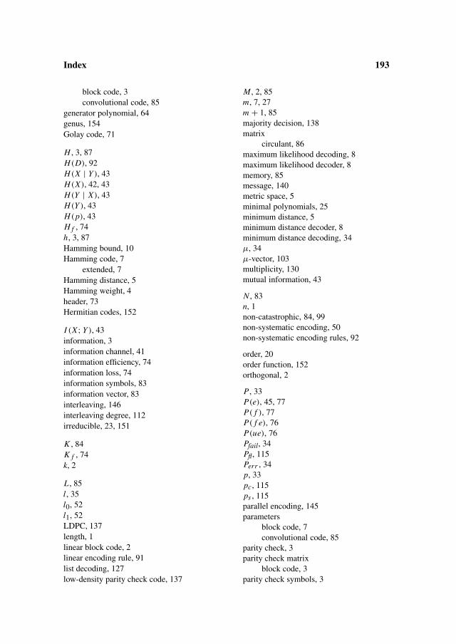
Index 193
block code, 3convolutional code, 85
generator polynomial, 64genus, 154Golay code, 71
H , 3, 87H(D), 92H(X | Y ), 43H(X), 42, 43H(Y | X), 43H(Y ), 43H(p), 43H f , 74h, 3, 87Hamming bound, 10Hamming code, 7
extended, 7Hamming distance, 5Hamming weight, 4header, 73Hermitian codes, 152
I (X; Y ), 43information, 3information channel, 41information efficiency, 74information loss, 74information symbols, 83information vector, 83interleaving, 146interleaving degree, 112irreducible, 23, 151
K , 84K f , 74k, 2
L , 85l , 35l0, 52l1, 52LDPC, 137length, 1linear block code, 2linear encoding rule, 91list decoding, 127low-density parity check code, 137
M , 2, 85m, 7, 27m + 1, 85majority decision, 138matrix
circulant, 86maximum likelihood decoding, 8maximum likelihood decoder, 8memory, 85message, 140metric space, 5minimal polynomials, 25minimum distance, 5minimum distance decoder, 8minimum distance decoding, 34µ, 34µ-vector, 103multiplicity, 130mutual information, 43
N , 83n, 1non-catastrophic, 84, 99non-systematic encoding, 50non-systematic encoding rules, 92
order, 20order function, 152orthogonal, 2
P, 33P(e), 45, 77P( f ), 77P( f e), 76P(ue), 76Pfail, 34Pfl, 115Perr , 34p, 33pc , 115ps , 115parallel encoding, 145parameters
block code, 7convolutional code, 85
parity check, 3parity check matrix
block code, 3parity check symbols, 3

194 Index
parity field, 73perfect code, 10, 98Plotkin bound, 15Poisson distribution, 34polynomial
degree, 22irreducible, 23minimal, 25
Polytrev’s bound, 38primitive element, 20probability, 33
of correct frame, 77of frame error, 76of undected error, 76event error, 106of decoding failure, 77
probability of frame loss, 115product code, 109�, 113punctured code, 90punctured dual code, 91puncturing, 15
Q(), 41Q(x), 51Q(x, y), 51Q0(x), 52Q1(x), 52q, 2quality, 76quasi-cyclic code, 86
R, 4, 83r, 4rate, 4received word, 4Reed-Solomon code, 50regular convolutional encoder, 88regular set, 98regular unit memory code, 93ρ, 100row distance, 89row tree code, 144
S, 57s, 4serial decoding, 110serial encoding, 112
shortened code, 90shortening, 15σ , 34source symbols, 73subfield subcode, 68symbol error probability, 115syndrome, 4syndrome decoder, 8systematic encoding, 3
t, 5tail-biting code, 86termination, 89ternary field, 20transfer frame, 74transmission efficiency, 74transmission overhead, 74tree, 139tree code, 140triangle inequality, 5
u, 83, 89u, 3UMC, 93unit memory code, 93
V , 2v(u), 83Varshamov-Gilbert bound, 6vector space, 2
wH , 4wmin , 5weight, 5weight distribution, 11weight enumerator, 11
Z , 38