Embed Size (px)
Citation preview
A Cost to Benefit Analysis of a Next Generation Electric Power
Distribution System
by
Apurva Raman
A Thesis Presented in Partial Fulfillment
of the Requirements for the Degree
Master of Science
Approved July 2015 by the
Graduate Supervisory Committee:
Gerald Heydt, Chair
George Karady
Raja Ayyanar
ARIZONA STATE UNIVERSITY
August 2015
i
ABSTRACT
This thesis provides a cost to benefit analysis of the proposed next generation of
distribution systems- the Future Renewable Electric Energy Distribution Management
(FREEDM) system. With the increasing penetration of renewable energy sources onto the
grid, it becomes necessary to have an infrastructure that allows for easy integration of
these resources coupled with features like enhanced reliability of the system and fast pro-
tection from faults. The Solid State Transformer (SST) and the Fault Isolation Device
(FID) make for the core of the FREEDM system and have huge investment costs.
Some key features of the FREEDM system include improved power flow control,
compact design and unity power factor operation. Customers may observe a reduction in
the electricity bill by a certain fraction for using renewable sources of generation. There
is also a possibility of huge subsidies given to encourage use of renewable energy. This
thesis is an attempt to quantify the benefits offered by the FREEDM system in monetary
terms and to calculate the time in years required to gain a return on investments made.
The elevated cost of FIDs needs to be justified by the advantages they offer. The result of
different rates of interest and how they influence the payback period is also studied. The
payback periods calculated are observed for viability. A comparison is made between the
active power losses on a certain distribution feeder that makes use of distribution level
magnetic transformers versus one that makes use of SSTs. The reduction in the annual
active power losses in the case of the feeder using SSTs is translated onto annual savings
in terms of cost when compared to the conventional case with magnetic transformers.
Since the FREEDM system encourages operation at unity power factor, the need
for installing capacitor banks for improving the power factor is eliminated and this re-

ii
flects in savings in terms of cost. The FREEDM system offers enhanced reliability when
compared to a conventional system. The payback periods observed support the concept of
introducing the FREEDM system. All cases studied in chapters one to five in this thesis
are tabulated in APPENDIX F.

iii
ACKNOWLEDGEMENTS
I would like to sincerely thank Dr. Gerald Heydt for giving me this amazing op-
portunity to pursue research and culminate my Master's experience with a thesis. He has
been very motivating, encouraging, patient with my questions and passionate about his
work. I have learnt a great deal professionally working under his guidance. I want to
thank Dr. George Karady and Dr. Raja Ayyanar for investing their time in being a part of
my defense committee and for their valuable suggestions.
This thesis would not have been possible without the funding provided by Na-
tional Science Foundation (NSF) and the FREEDM center. I am honored to be a part of
the Electrical Engineering department at Arizona State University. I want to thank all the
staff members, my academic advisors and teachers who have taught me a wide range of
courses specializing in power systems that have sharpened my knowledge of power sys-
tem concepts.
I dedicate this thesis to my parents, late Mr. V.S. Raman and Mrs. Lata Raman as
well as my elder brother Mr. Aditya Raman who have been constant pillars of strength
and a major reason behind me pursuing my Master's. Without their support, motivation
and confidence in my abilities, I could not have reached this stage. Lastly, I would like to
thank all my relatives, friends and colleagues who have helped me at every step of my
life in shaping me into a strong individual.
iv
TABLE OF CONTENTS
Page
LIST OF TABLES ........................................................................................................... viii
LIST OF FIGURES ........................................................................................................... ix
NOMENCLATURE ......................................................................................................... xii
CHAPTER
1 THE FREEDM SYSTEM: COSTS AND BENEFITS .............................................1
Motivation ..............................................................................................................1
Project Objectives ...................................................................................................1
Cost to Benefit Analysis .........................................................................................2
The FREEDM System ............................................................................................5
Cost and Attributes of Distribution Transformers ..................................................8
The Solid State Transformer ..................................................................................9
Fault Isolation Devices .........................................................................................12
Principal Assumptions Made in the Cost to Benefit Analysis ..............................14
Organization of this Thesis ...................................................................................16
2 ACTIVE POWER LOSSES IN DISTRIBUTION TRANSFORMERS ................18
Introduction ..........................................................................................................18
Simulation Studies ................................................................................................18
Example Evaluation of Losses in a 36 kVA Magnetic Transformer................... 20
v
CHAPTER Page
Scaled Loading on the 36 kVA Transformer for Every Hour Using ERCOT Load
Data................ ......................................................................................................22
Example Evaluation of Losses in a 36 kVA SST ................................................23
Annual Energy Loss for a 36 kVA Magnetic Transformer .................................25
Annual Energy Loss: 36 kVA SST ......................................................................25
An algorithm for Calculation of Annual Energy Loss in Transformers..............26
Calculation Summary for Transformer Active Power Losses ..............................26
3 ACTIVE POWER LOSSES IN DISTRIBUTION PRIMARY CONDUCTORS ..32
A Test Bed for the Evaluation of Active Power Losses.......................................32
Example Evaluation of Feeder Losses with 36 kVA Magnetic Transformers .....33
Example Evaluation of Feeder Losses with 36 kVA SSTs ..................................35
Annual Energy Loss in Feeder: Using 36 kVA Magnetic Transformers .............36
Annual Energy Loss in Feeder: Using 36 kVA SSTs ..........................................36
Algorithm for Calculation of Annual Energy Loss in the Feeder ........................37
Calculation of Feeder Losses with Capacitor Bank Compensation.................. ...37
Calculation of Cost of Capacitor Banks to Improve Power Factor of Feeder ......39
Calculation Summary of Line and Transformer Active Power Losses................42
Summary of Results..............................................................................................42
4 RELIABILITY OF SERVICE TO CUSTOMERS AND NUMBER OF FIDs. .....45
vi
CHAPTER Page
Service Reliability ................................................................................................45
Reliability Calculations for Configuration A .......................................................47
A Closed Form Expression for E(E) for Configuration A ....................................52
Summary of Results for Configuration A ............................................................52
Reliability Calculations for Configuration B .......................................................53
A Closed Form Expression for E(E) for Configuration B ....................................59
Summary of Results for Configuration B .............................................................59
Results for Configuration A and Configuration B ...............................................59
Comparison of SAIFI between a Certain Base Case and FREEDM System .......60
Solid State Fuses as an Alternative to FID ...........................................................61
5 CALCULATION AND DISCUSSION OF PAYBACK PERIODS ......................63
Introduction ..........................................................................................................63
Calculation of Payback Period without Considering Rate of Interest ..................65
Calculation of Payback Period Considering Rate of Interest ...............................66
Results ..................................................................................................................67
Summary and Conclusions...................................................................................67
6 CONCLUSIONS AND RECOMMENDATIONS .................................................69
Conclusions ..........................................................................................................69
Recommendations and Future Work ....................................................................70
vii
CHAPTER Page
REFERENCES ..................................................................................................................72
APPENDIX
A: LOSS CALCULATION FOR A 36 KVA MAGNETIC TRANSFORMER .........76
B: LOSS CALCULATION FOR A 36 KVA SST ......................................................80
C: ANNUAL ENERGY LOST IN FEEDER USING DISTRIBUTION LEVEL
MAGNETIC TRANSFORMERS AND SSTs............................................................83
D: CURVE APPROXIMATION OF RELIABILITY CALCULATIONS FOR
CONFIGURATIONS A AND B .................................................................................86
E: CALCULATION OF PAYBACK PERIOD WITH INTEREST RATES FOR
CONFIGURATIONS A AND B .................................................................................88
F: SUMMARY OF ALL THE TEST CASES USED .................................................92
viii
LIST OF TABLES
Table Page
1.1 Mapping of FREEDM Features/Functions to Benefits............................................7
2.1 Summary of Energy Loss and Cost of Energy Loss Obtained for 36 kVA Con-
ventional Transformer............................................................................................29
2.2 Summary of Energy Loss and Cost of Energy Loss Obtained for 36 kVA SST...30
3.1 A Summary of Cost of Active Power Losses in Feeder and Transformers
with and without Addition of Capacitor Banks.....................................................44
4.1 Test Cases for Configuration A ........................................................................ ....46
4.2 Test Cases for Configuration B............................................................................. 46
4.3 Results for Configuration A and B ....................................................................... 60
5.1 Calculation Summary of Payback Period for Both Configurations with and with-
out Rate of Interest ....... .........................................................................................68
F.1 Summary of all the Cases Studied in this Thesis .................................................. 95
ix
LIST OF FIGURES
Figure Page
1.1 The Envisioned FREEDM Distribution System ......................................................2
1.2 A Pictorial of Investments and Functionalities ....................................................... 4
1.3 FREEDM System.................................................................................................... 5
1.4 Topology Classification of an SST ....................................................................... 10
1.5 Potential Application of an SST in Future Electrical System ............................... 12
1.6 Application of SST in a Prototype Distribution System ....................................... 12
1.7 The CBEMA Curve .............................................................................................. 14
2.1 A Pictorial of the Approach Used to Evaluate Transformer Losses in Distribution
System ................................................................................................................... 19
2.2 Distribution System Assumed for Loss Calculations for a Single 36 kVA Trans-
former, T2, Serving 4-5 Residences ..................................................................... 19
2.3 Ercot Loading for the Year 2013 as Divided by Peak Load of the Year. ............. 21
2.4 A Pictorial of a 0.72 MVA Feeder showing 20 Distribution Transformers ......... 21
2.5 Algorithm for Calculation of Annual Active Power Losses in a 36 kVA Magnetic
Transformer........................................................................................................... 27
2.6 Algorithm for Calculation of Annual Active Power Losses in a 36 kVA SST .... 28
2.7 A Summary of Annual Energy Lost in a 36 kVA Magnetic Transformer Tabulated
in Table 2.1(MWh/Year) ...................................................................................... 29
2.8 A Summary of Annual Cost of Energy Lost in a 36 kVA Magnetic Transformer
Tabulated in Table 2.1($/Year) ............................................................................. 30
x
Figure Page
2.9 A Summary of Annual Energy Lost in a 36 kVA SST Tabulated in Table 2.2
(MWh/Year) .......................................................................................................... 31
2.10 A Summary of Annual Cost of Energy Lost in a 36 kVA SST Tabulated in
Table 2.2 ($/Year)..................................................................................................31
3.1 A Pictorial of the Test Bed Feeder Used for Active Power Loss Calculations .... 32
3.2 Algorithm For Calculation Annual Cost of Energy Loss in a Distribution
Feeder.....................................................................................................................37
3.3 Annual Cost of Energy Lost in the Feeder as well as Transformers .................... 43
4.1 A Pictorial of the Configurations Used to Study Reliability of Service to
Customers ............................................................................................................. 45
4.2 A Pictorial of the System Used to Calculate Reliability of Service Due to Faults
with 2n+2 Number of Fids in Service (Case 1A) ................................................. 48
4.3 A Pictorial of the System Used to Calculate Reliability of Service Due to Faults
with (2n+1) Number of FIDs in Service (Case 2A) .............................................. 49
4.4 A Pictorial of the System Used to Calculate Reliability of Service Due to Faults
with (2n) FIDs in Service (Case 3A) .................................................................... 50
4.5 A Pictorial Of The System Used To Calculate Reliability Of Service Due To
Faults With 3 FIDs In Service (Case 4A) ............................................................. 51
4.6 A Pictorial of the System Used to Calculate Reliability of Service Due to Faults
with 2 FIDs in Service (Case 5A) ......................................................................... 52
4.7 A Graph of Number of Customers Served Versus Number of FIDs in Service for
Configuration A .................................................................................................... 53
xi
Figure Page
4.8 A Pictorial of the System Used to Calculate Reliability of Service Due to Faults
with (n+2) Number of FIDs in Service (Case 1B) ............................................... 54
4.9 A Pictorial of the System Used to Calculate Reliability of Service Due to Faults
with (n+1) FIDs in Service (Case 2B)...................................................... ...........55
4.10 A Pictorial of the System Used to Calculate Reliability of Service Due to Faults
with n FIDs In Service (Case 3B) ........................................................................57
4.11 A Pictorial of the System Used to Calculate Reliability of Service Due to Faults
with 3 FIDs in Service (Case 4B) .........................................................................57
4.12 A Pictorial of the System Used to Calculate Reliability of Service Due to Faults
with 2 FIDs in Service (Case 5B) .........................................................................58
4.13 A Graph of Number of Customers Served Versus Number of FIDs in Service for
Configuration B ................................................................................................. 61
4.14 SAIFI Comparison of a Conventional Residential Feeder Versus the
FREEDM System...............................................................................................61
xii
NOMENCLATURE
a Constant used in Third Degree Curve Approximation of Expected Num-
ber of Customers Served
b Constant used in Third Degree Curve Approximation of Expected Num-
ber of Customers Served
Benefit Total Benefits Associated with the FREEDM System
BIL Basic Insulation Level
c Constant used in Third Degree Curve Approximation of Expected Num-
ber of Customers Served
C Capacitance in µF
CBEMA Computer Business Equipment Manufacturer's Association
Cost Total Costs Related to the FREEDM System
CP Annual Reduction in Cost due to Elimination of Installation of Capacitor
Banks
d Constant used in Third Degree Curve Approximation of Expected Num-
ber of Customers Served
DESD Distributed Energy Storage Devices
DGI Distributed Grid Intelligence
DLMP Distribution Locational Marginal Price
DRER Distributed Renewable Energy Resource
E Number of Customers Served
E(.) Expectation
ERCOT Electric Reliability Council of Texas
freq Frequency in Hertz
f Variable used in Iterative Calculations of Payback Periods

xiii
f0 Variable used in Iterative Calculations of Payback Periods
f1 Variable used in Iterative Calculations of Payback Periods
F Total Cost of Fault Interruption Devices Installed in a given Configura-
tion of System
FID Fault Isolation Device
FO Forced Oil Cooled Units
FREEDM Future Renewable Electric Energy Delivery and Management
G Subsidy of 10 % of the Customer's Annual Bill to Encourage Utilization
of the FREEDM System
H Annual Savings in Electricity Bill per Customer due to use of Renewa-
bles
i Annual Rate of Interest in %
I Current Flowing in the Conductors
IEC International Electrotechnical Commission
l Length of the Feeder
L Annual Reduction in Cost of Active Power Losses When Compared with
a System Consisting of Conventional Transformers
LOLE Loss of Load Energy
Ln, Lm, Lk Load at Points n, m and k
MOSFET Metal Oxide Semiconductor Field Effect Transistor
n Number of Customers served
n'
Payback Period in Years
n0 Variable used in Iterative Calculations of Payback Periods
n1 Variable used in Iterative Calculations of Payback Periods
xiv
NEMA National Electrical Manufacturers Association
pf Power Factor
P Active Power
PSERC Power Systems Engineering Research Center
Plost Active Power Losses
Pmax Maximum Loading in Watts for a Given Year
Pscaled Scaled Loading of Transformer
Q Reactive Power in kVAr
Qcompensation Reactive Power to be Compensated while Improving Power Factor
r RMS Error in Curve Approximation
R Resistance of the Conductors
RB Value of Enhanced Reliability Benefit for all the Customers Served in a
Given System for a Given Year
RPS Renewable Portfolio Standards
Rsection Resistance of a Given Line Section
S Total Cost of Solid State Transformers Installed in a Given Configura-
tion of System
SAIDI System Average Interruption Duration Index
SAIFI System Average Interruption Frequency Index
SST Solid State Transformer
US DoE Unites States Department of Energy
V Variable Used in Third Degree Curve Approximation of Expected Num-
ber of Customers Served that Represents Number of Fault interruption
devices in service
Vop Operating Voltage at a Given Bus

xv
y Constant Used for Calculating the Value of kVARs Required to Improve
the Operating Power Factor of the Feeder
Frequency in rad/s
1
CHAPTER 1 THE FREEDM SYSTEM: COSTS AND BENEFITS
1.1 Motivation
This thesis relates to electric power distribution systems. With the increasing need
for integration of renewable energy resources, it is necessary that an architecture that fa-
cilitates some automated features will be used. These automated features include: 'plug
and play' of distributed renewable energy resources and storage devices, central monitor-
ing and control and advanced instrumentation [1]. The next generation of distribution
system is exemplified by the Future Renewable Electric Energy Delivery and Manage-
ment (FREEDM) system which uses solid state transformers and other semiconductor
switched distribution system components to achieve the cited features. The automated
features come with costs. The main motivation of this thesis relates to the study of the
costs versus benefits of a solid state controlled power distribution system. The FREEDM
system shall be used as the test bed for the study.
1.2 Project Objectives
The FREEDM system has been envisioned as the next generation of power distri-
bution system architecture laying emphasis on solid state transformers (SSTs). While this
system has many obvious advantages to offer in terms of enhancing control of the power
distribution grid, these controls come with investment as well. This thesis attempts to
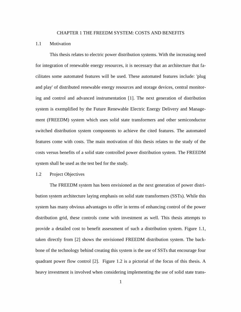
provide a detailed cost to benefit assessment of such a distribution system. Figure 1.1,
taken directly from [2] shows the envisioned FREEDM distribution system. The back-
bone of the technology behind creating this system is the use of SSTs that encourage four
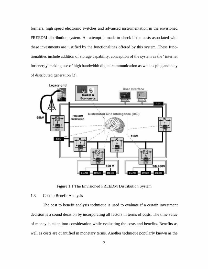
quadrant power flow control [2]. Figure 1.2 is a pictorial of the focus of this thesis. A
heavy investment is involved when considering implementing the use of solid state trans-
2
formers, high speed electronic switches and advanced instrumentation in the envisioned
FREEDM distribution system. An attempt is made to check if the costs associated with
these investments are justified by the functionalities offered by this system. These func-
tionalities include addition of storage capability, conception of the system as the ' internet
for energy' making use of high bandwidth digital communication as well as plug and play
of distributed generation [2].
Figure 1.1 The Envisioned FREEDM Distribution System
1.3 Cost to Benefit Analysis
The cost to benefit analysis technique is used to evaluate if a certain investment
decision is a sound decision by incorporating all factors in terms of costs. The time value
of money is taken into consideration while evaluating the costs and benefits. Benefits as
well as costs are quantified in monetary terms. Another technique popularly known as the

3
life cycle analysis is a method used to assess measurable quantities of a particular system
through its entire cycle from cradle to grave [3]. At times it becomes difficult to quantify
all factors in terms of a number for the purpose of analysis and the data for the same may
not be easily available or accurate. In order to decide which one of the two methods
should be executed for the analysis of the prototype distribution system suggested, certain
advantages and disadvantages of both the methods are discussed. The following are cer-
tain advantages and disadvantages of using the cost to benefit analysis method [4]:
Advantages of the cost to benefit analysis method:
1. Commonly used in electrical power industry.
2. Gives a calculated estimate of payback period to determine feasibility.
3. Easy and fast method to recognize if a project is viable.
Disadvantages of the cost to benefit analysis method:
1. Certain factors are difficult to quantify in dollars- pollution, time and human
life.
2. Difficult to assess indirect benefits.
3. Accuracy – if inaccurate it results in false estimation of payback period there-
by risking project feasibility.
4. Uncertainty in data and risk factors may add to the costs.
5. Short term analysis.
The following are certain advantages and disadvantages of using the life cycle analysis
method [3]:
Advantages of the life cycle analysis method:
4
Factors in all the costs right from initial costs to the operation, maintenance and decom-
mission costs.
1. Detailed analysis of costs and benefits over the entire life cycle of the project
(cradle to grave cost).
Disadvantages of the life cycle analysis method:
1. It may get difficult to limit the scope of the project at times.
2. Uncertainty in data.
3. Tricky to envisage the risks and uncertainties in future.
4. It is difficult to predict the value of dollar in future.
5. Technology may become obsolete.
The cost to benefit method is a straightforward and fast method to recognize if a
project is viable and since it also gives a calculated estimate of the payback period, it is
favorable to proceed with the cost to benefit analysis for the suggested FREEDM distri-
bution system. References [21] – [23] further document cost to benefit analysis in power
distribution systems.
Figure 1.2 A Pictorial of Investments and Functionalities
5
1.4 The FREEDM System
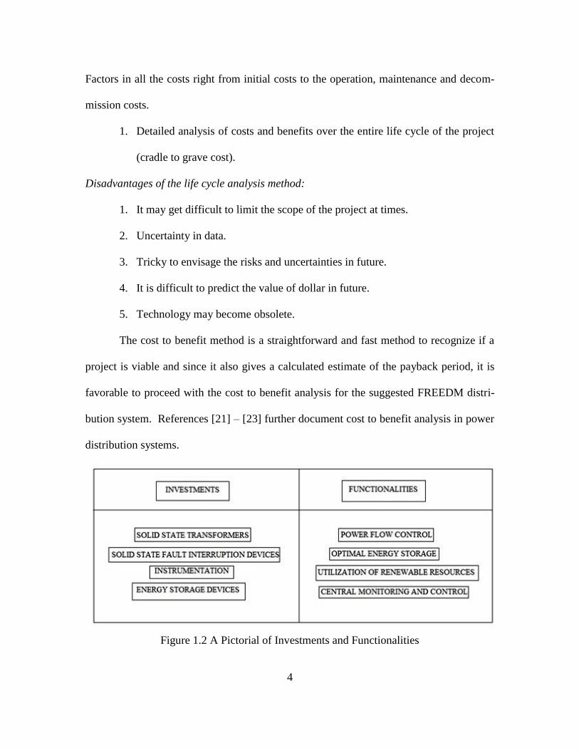
Figure 1.3, inspired from [11] shows the FREEDM distribution system which im-
plements the use of an SST instead of a conventional magnetic transformer as the distri-
bution level transformer. In addition to the blocks shown in Figure 1.3, Distributed Grid
Intelligence (DGI) as well as Distributed Energy Storage Devices (DESD) control the
effective functioning of the FREEDM system. The FREEDM system ensures seamless
integration of renewable energy resources and facilitates storage of energy. High fre-
quency isolation, AC/AC converters and high power converters have made the power
grid very robust and active [6]. The zonal DC micro grid concept being applied to the
FREEDM system is highlighted in [8]. The integration issues in the DC micro grid and
SST are analyzed and measures are suggested to minimize burden on the existing AC
grid. The problem with the existing system is that utilization of power converters is very
low in current transmission and distribution systems [7].
Figure 1.3 FREEDM System

6
To evaluate the benefits of the system indicated in Figure 1.3, an effort is made to
quantify them in terms of cost as follows:
Costs easily quantifiable:
Elimination of capacitors for reactive power compensation can be translated as a
reduction in cost for the FREEDM system.
Reduction in size and weight by comparison of prototype SST with a convention-
al low frequency transformer.
Material and parts cost.
Cost is quantifiable if a target renewable level is mandated or there are other
mandates to be implemented.
Savings due to improvement in load factor.
For some cases, loss of load energy (LOLE) is quantifiable and the FREEDM sys-
tem could reduce LOLE.
Reduced shipping costs.
Potential for reduced manufacturing costs.
Costs quantifiable with difficulty:
Costs associated with reduction of harmonic currents in SST supply (harmonic fil-
tering).
Labor and equipment costs involved in manufacturing SSTs.
Control and monitoring equipment for two way power flow.
Costs due to political and sociological influences on the project.
Potential to achieve environmental goals.

7
Achieving high safety standards via fast interruption and protection in comparison
to conventional system using magnetic transformers.
The FREEDM project was funded mainly by the National Science Foundation as
an Engineering Research Center. References [1], [2], [6] and [10] document the main ef-
forts of the FREEDM project. Table 1.1 maps the potential features and functions of the
proposed FREEDM system as benefits as follows and is taken directly from [31].
Table 1.1 Mapping of FREEDM Features/Functions to Benefits
Benefits
FREEDM system fea-
tures/functions Economics
Reliability
& power
quality Societal
Energy
security
Renewable integration
· Manage high penetration
· Plug & play
Enhanced system protection
· Looped primary
· Fast protection with FID
Enhanced fault protection
· Fault locating, isolation, service
restoration
Real time load monitoring &
management
· Regulate service voltage
Customer participation
· DGI- price signals DLMP, de-
mand side management
Enhanced system control
· DGI: power & energy manage-
ment
· DGI: volt/var control
Resiliency
· Microgrid at node, feeder sec-
tion, whole feeder
8
1.5 Cost and Attributes of Distribution Transformers
There exist few direct quantitative comparisons between a magnetic transformer
and an SST of the same rating. This is because there is, in reality, no solid state trans-
former in production and for sale in large volume quantity. Nonetheless, some estimates
can be made but it is important to admit that there is uncertainty in the estimates.
An attempt is made to provide a comparison between the volume, weight and cost
of a 1000 kVA, 10 kV/ 400 V solid state transformer and a magnetic transformer of the
same rating in [5]. The estimated values of cost only take into account the lower bound
values of material costs, a major part of which is that of hardware. SST costs exclude in-
stallation costs, cost of protection equipment and final assembly costs. Reference [5]
gives a comparison of losses in the transformers per kVA, material costs per kVA, vol-
ume per kVA as well as the weight per kVA. It was observed that the SST was 5 times
more expensive when compared to the conventional transformer with 3 times higher loss-
es. The weight was almost the same but the volume of the SST was only 80% of that of a
conventional transformer.
As the losses in an SST are generally higher as compared to those in a magnetic
transformer, the efficiencies of SSTs will be significantly lower than those of conven-
tional transformers. This is specially the case for low operational loading. In spite of this,
“SSTs can act as energy routers of a future smart grid” [5]. SSTs offer a high degree of
intelligent control of power flows. This is indispensable considering recent developments
in the fields of smart grid and distributed energy generation systems. SSTs are also useful
in integrating renewable energy sources into distribution systems. SST is an emerging
technology for the future of distribution systems and smart grids [6]. The SST offers AC

9
as well as DC links that enhance the supply of power and allow both AC and DC net-
works to easily communicate with the SST [7]. Researchers involved in developing SSTs
are interested in identifying which topology will be best suitable for field applications
and are involved with improving and enhancing performance of high power converters.
SSTs can help in replacing the oil used in conventional magnetic transformers and can
enhance the functionality and power quality to justify its cost. This thesis attempts to
quantify the costs and benefits and tries to prove if this is in fact possible.
An investigation on the application issue of SSTs in the future electrical grid is
carried out in [8]. It attempts to explain how integrating multiple functionalities in the
SST may justify its cost. It is suggested that increasing the switching frequency can ena-
ble reduction in size of SSTs in [9]. High voltage insulation needs to be carefully de-
signed. The specified requirements for SST application at high frequency and voltage
were optimized and a prototype achieving an efficiency of 96.9 % was suggested. Figure
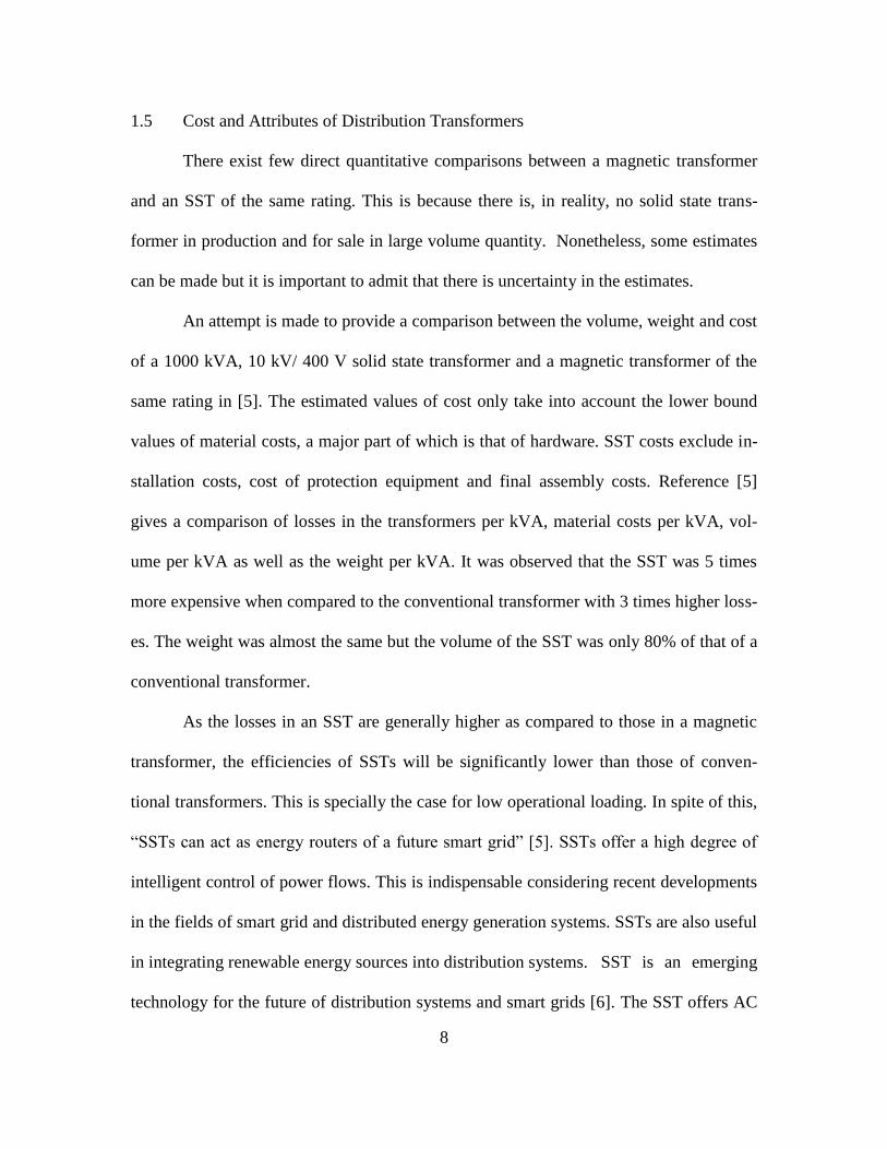
1.4 shows the classification of different topologies of SSTs. The type D topology is sug-
gested to be used extensively in the field applications of SST. Figures 1.5 shows the po-
tential application of SST in the future electrical grid. Figures 1.4 and 1.5 were inspired
by [7].
1.6 The Solid State Transformer
SSTs are an evolving topic of discussion in terms of ongoing research within the
realms of improving the existing state of distribution systems. They can play an important
role when used in smart grid applications to improve flexibility and controllability of the
system. An SST may be defined as follows: “A solid state transformer is a collection of
high-powered semiconductor components, conventional high-frequency transformers and
10
control circuitry which is used to provide a high level of flexible control to power distri-
bution networks” [10].
Figure 1.4 Topology Classification of an SST
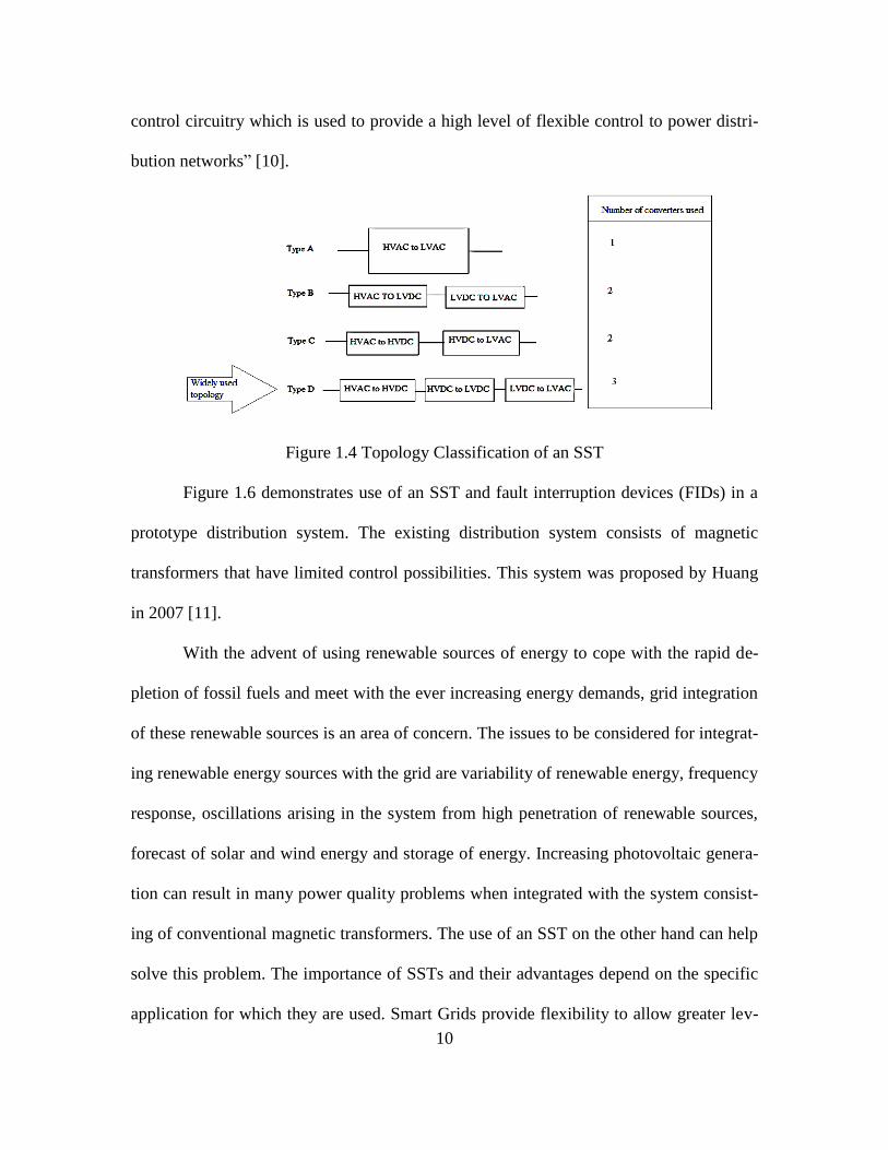
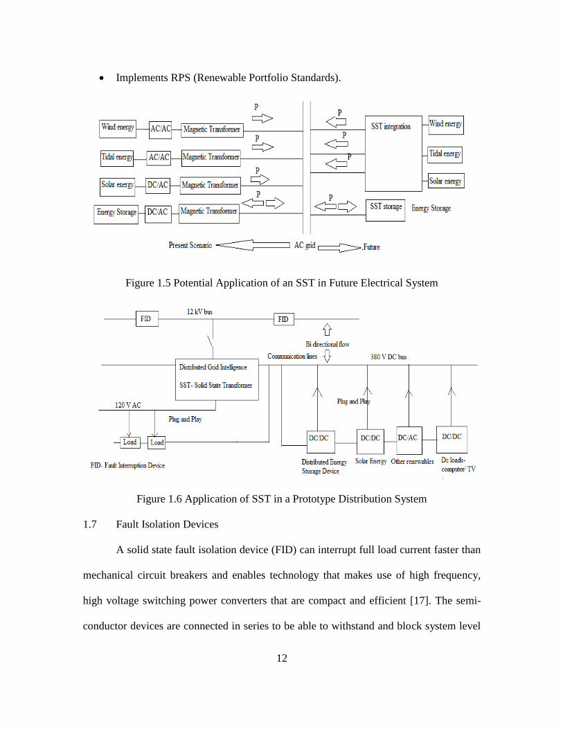
Figure 1.6 demonstrates use of an SST and fault interruption devices (FIDs) in a
prototype distribution system. The existing distribution system consists of magnetic
transformers that have limited control possibilities. This system was proposed by Huang
in 2007 [11].
With the advent of using renewable sources of energy to cope with the rapid de-
pletion of fossil fuels and meet with the ever increasing energy demands, grid integration
of these renewable sources is an area of concern. The issues to be considered for integrat-
ing renewable energy sources with the grid are variability of renewable energy, frequency
response, oscillations arising in the system from high penetration of renewable sources,
forecast of solar and wind energy and storage of energy. Increasing photovoltaic genera-
tion can result in many power quality problems when integrated with the system consist-
ing of conventional magnetic transformers. The use of an SST on the other hand can help
solve this problem. The importance of SSTs and their advantages depend on the specific
application for which they are used. Smart Grids provide flexibility to allow greater lev-

11
els of penetration of variable renewable energy sources such as wind and solar even
without the addition of energy storage [12]. Thus, SSTs serve their purpose well in Smart
Grid applications and offer the following advantages when installed in distribution sys-
tems:
Fast interruption and protection of faults.
AC-DC type SSTs may have some efficiency benefit.
Integrate energy storage.
Maintain unity power factor.
Load transient and harmonic regulation (no/very low harmonic currents in SST
supply currents).
Smaller in size and weight as compared to conventional magnetic transformers.
Potential for fast installation.
Central monitoring and control via instrumentation.
Encourage renewable energy.
Protect load from power system disturbances.
Voltage harmonic and sag compensation on the load side.
Can take DC input from solar and batteries.
Help in levelizing load and improving load factor. (For e.g. by varying the load
voltage)
Potential for support of the grid using distributed generation.
"Next Generation” of distribution system.
Potential for operating “off grid”.
12
Implements RPS (Renewable Portfolio Standards).
Figure 1.5 Potential Application of an SST in Future Electrical System
Figure 1.6 Application of SST in a Prototype Distribution System
1.7 Fault Isolation Devices
A solid state fault isolation device (FID) can interrupt full load current faster than
mechanical circuit breakers and enables technology that makes use of high frequency,
high voltage switching power converters that are compact and efficient [17]. The semi-
conductor devices are connected in series to be able to withstand and block system level

13
high voltages. According to [18], to validate the use of fault interruption devices in medi-
um voltage distribution systems, a system with FID model is subjected to simulated tests
for continuous current carrying capacity, rated fault current interruption and lightning
impulse withstand tests. This semiconductor device driven power electronic interface fa-
cilitates connection of distributed generation sources to the network. The operation of the
interface devices can be disrupted by transients and over-voltages caused in the system
due to fault conditions. This disruption can be faster than the time taken by conventional
circuit breakers to operate. The FID on the contrary provides high speed interruption to
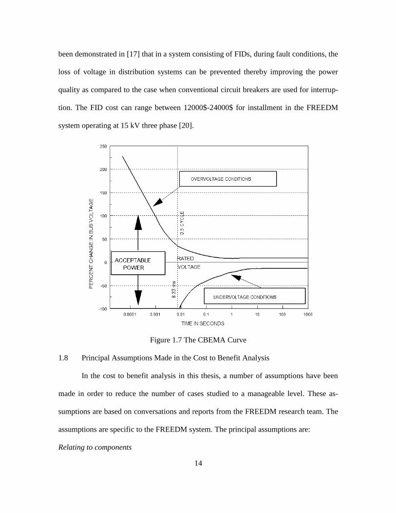
help solve the issue of loss of power during faults [18]. The basic philosophy of the use
of a very high speed FID is to limit the duration of a fault in the distribution primary. As
an example, the Computer Business Equipment Manufacturer's Association (CBEMA)
curve allows a 100% low voltage (i.e. total outage) for one half cycle. This is
second
in a 60 Hz system. References [34]-[35] document the CBEMA curve and its applica-
tions. Figure 1.7 shows the CBEMA curve [36].
Reference [19] addresses the timely issues in modeling of and specifying the se-
lection criteria for FIDs to be used in medium voltage power distribution systems. Major
drawbacks of installing FIDs in place of mechanical circuit breakers are the high material
costs and on-state losses (switching losses). Reference [19] validates selection of a suita-
ble topology of FID installation and the feasibility of the proposed topology through sim-
ulations.
Thus, FIDs interrupt fault currents within a few 100 microseconds as compared to
about 12 milliseconds for even the fastest operating conventional circuit breaker. It has
14
been demonstrated in [17] that in a system consisting of FIDs, during fault conditions, the
loss of voltage in distribution systems can be prevented thereby improving the power
quality as compared to the case when conventional circuit breakers are used for interrup-
tion. The FID cost can range between 12000$-24000$ for installment in the FREEDM
system operating at 15 kV three phase [20].
Figure 1.7 The CBEMA Curve
1.8 Principal Assumptions Made in the Cost to Benefit Analysis
In the cost to benefit analysis in this thesis, a number of assumptions have been
made in order to reduce the number of cases studied to a manageable level. These as-
sumptions are based on conversations and reports from the FREEDM research team. The
assumptions are specific to the FREEDM system. The principal assumptions are:
Relating to components

15
Switching losses in an SST are five times the active power losses of the I2R losses
in the semiconductor switches.
Two loss cases are assumed for the SST, namely a 5% loss and a 1% loss (at 75%
loading, the US Department of Energy standard).
The cost of distribution class capacitors is 3.54$/kVAr (based on a 10 microfarad
unit, 15 kV line – line class, single phase unit priced). To span the possible costs
for capacitors, 35.4$/kVAr was also considered.
The cost of FREEDM designed fault interruption devices (FIDs) was assumed to
lie between 1000$-10000$ (assuming technology matures and a mass scale bulk
order is placed for commercialization of the FREEDM system).
The cost of the SST was estimated at 67$/kVA, single phase unit (estimated from
the FREEDM research team).
The distribution primary conductor was assumed to be No. 2 Aluminum as docu-
mented in [16].
The life of capacitors was taken to be 10 years.
The life of an SST as well as an FID was taken to be 12 years.
The life of a magnetic transformer was taken to be 20 years.
Relating to feeder design
The FREEDM feeder was assumed to have 2 sources of generation at the two
ends of the feeder, 20 distribution transformers, 36 kVA each, with three to four
individual services for each transformer, totaling 0.72 MVA of the total load.
The load along the FREEDM feeder was assumed to be evenly distributed along
the feeder.

16
The FREEDM feeder was taken to be 10 miles long.
Relating to the feeder load
The load data was a scaled version of assumed typical US residential load data.
These load data were taken from the Electric Reliability Council of Texas
(ERCOT). The data used were for the entire state of Texas, and appropriate scal-
ing was used to obtain the FREEDM feeder loading.
The load power factor was taken over a range of values in order to span actual
load conditions, namely 60 to 100%.
1.9 Organization of this Thesis
Chapter 1 of this thesis discusses the motivation behind this research and outlines
the project objectives. It explains how a cost to benefit analysis is conducted and how it
can be applied to the FREEDM system. A brief introduction about FIDs and SSTs is giv-
en. The principal assumptions made in the cost to benefit analysis are also discussed.
Chapter 2 discusses active power losses in transformers, magnetic as well as solid state
and compares the annual active power losses for a 36 kVA magnetic transformer with
that for a 36 kVA SST. The ERCOT loading data for the year 2013 is scaled to obtain the
value of loading on a single 36 kVA transformer. The annual energy loss is calculated for
both the transformers and compared. Chapter 3 discusses active power losses in a 10 mile
long feeder fed from both the ends. The active power losses in the feeder are calculated
for two cases: one with 36 kVA magnetic transformers at the 20 load points and the other
with 36 kVA SSTs at the 20 load points. The annual energy lost in the feeder is compared
for these two cases. Cost of installing capacitors banks to improve operating power factor
of the feeder are calculated for the conventional system.

17
Chapter 4 establishes the relation between the reliability of service to customers
versus the number of FIDs installed in the system for two different configurations- A and
B. A closed form expression for the expected number of customers served is calculated
for both the configurations and compared. A comparison of SAIFI between a radial con-
ventional system and the FREEDM system is also provided. Chapter 5 calculates the
payback period required to earn a return on investments for the FREEDM system by
quantifying the benefits calculated in Chapters 2, 3 and 4 in terms of cost. It also discuss-
es how different rates of interest affect the payback periods. Chapter 6 summarizes the
results obtained in Chapter 5 as conclusions and explains why the FREEDM system is
certainly a viable project based on the cost to benefit analysis. Appendices A through F
support the analysis done in Chapters 2 through 5.
18
CHAPTER 2 ACTIVE POWER LOSSES IN DISTRIBUTION TRANSFORMERS
2.1 Introduction
This chapter focuses on active power losses in transformers. The objective of this
chapter is to compare the active power lost in an SST versus the active power lost in a
conventional magnetic transformer of the same rating. MATLAB simulations are done to
arrive at the results. References [24] to [28] help in understanding the steps involved in
calculation of active power losses in a conventional magnetic transformer.
2.2 Simulation Studies
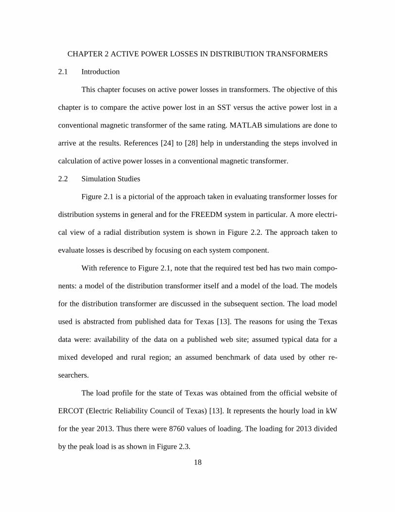
Figure 2.1 is a pictorial of the approach taken in evaluating transformer losses for
distribution systems in general and for the FREEDM system in particular. A more electri-
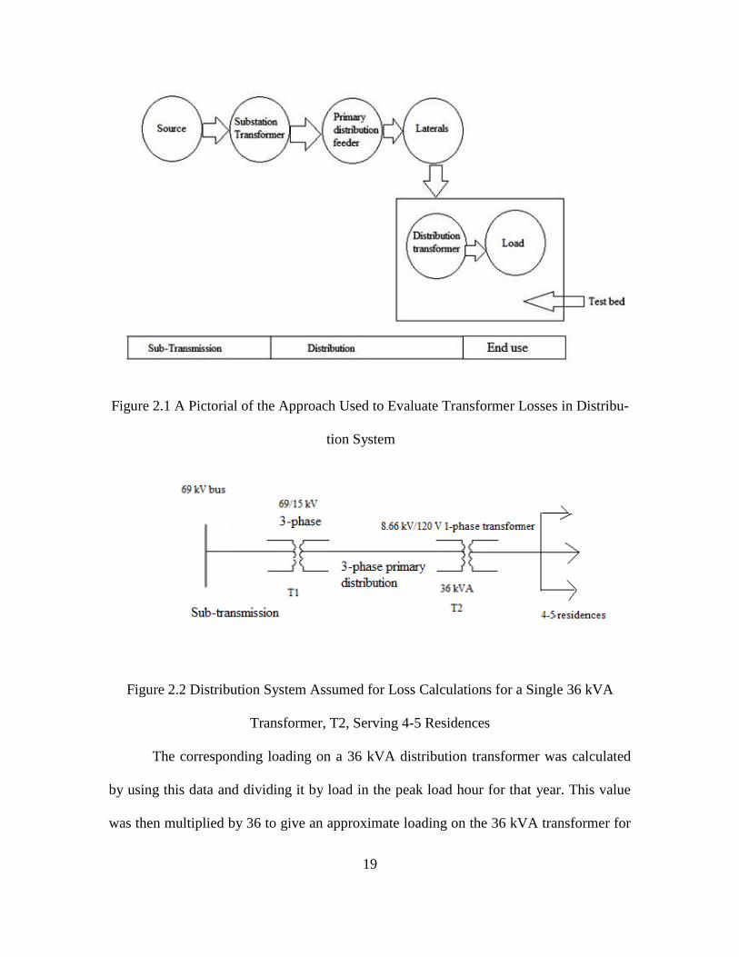
cal view of a radial distribution system is shown in Figure 2.2. The approach taken to
evaluate losses is described by focusing on each system component.
With reference to Figure 2.1, note that the required test bed has two main compo-
nents: a model of the distribution transformer itself and a model of the load. The models
for the distribution transformer are discussed in the subsequent section. The load model
used is abstracted from published data for Texas [13]. The reasons for using the Texas
data were: availability of the data on a published web site; assumed typical data for a
mixed developed and rural region; an assumed benchmark of data used by other re-
searchers.
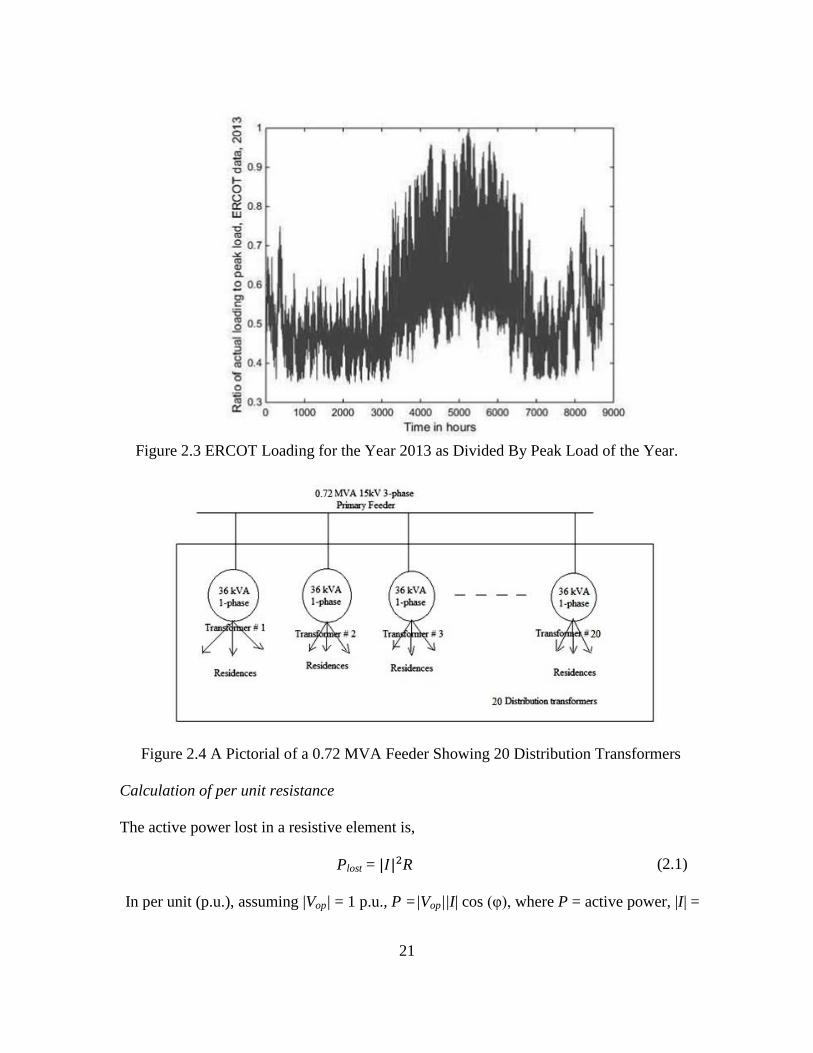
The load profile for the state of Texas was obtained from the official website of
ERCOT (Electric Reliability Council of Texas) [13]. It represents the hourly load in kW
for the year 2013. Thus there were 8760 values of loading. The loading for 2013 divided
by the peak load is as shown in Figure 2.3.
19
Figure 2.1 A Pictorial of the Approach Used to Evaluate Transformer Losses in Distribu-
tion System
Figure 2.2 Distribution System Assumed for Loss Calculations for a Single 36 kVA
Transformer, T2, Serving 4-5 Residences
The corresponding loading on a 36 kVA distribution transformer was calculated
by using this data and dividing it by load in the peak load hour for that year. This value
was then multiplied by 36 to give an approximate loading on the 36 kVA transformer for

20
every hour of the year 2013. This meant that the peak load hour would load the trans-
former 100%, that is, the loading would be 36 kVA for the peak load hour.
The losses in a 36 kVA conventional transformer as well as SST of the same rat-
ing were calculated using the above obtained values of loading on the transformer. The
transformer T2 is the transformer of interest for calculation of losses. Two cases are con-
sidered: T2 is a magnetic transformer and T2 is an SST.
2.3 Example Evaluation of Losses in a 36 kVA Magnetic Transformer
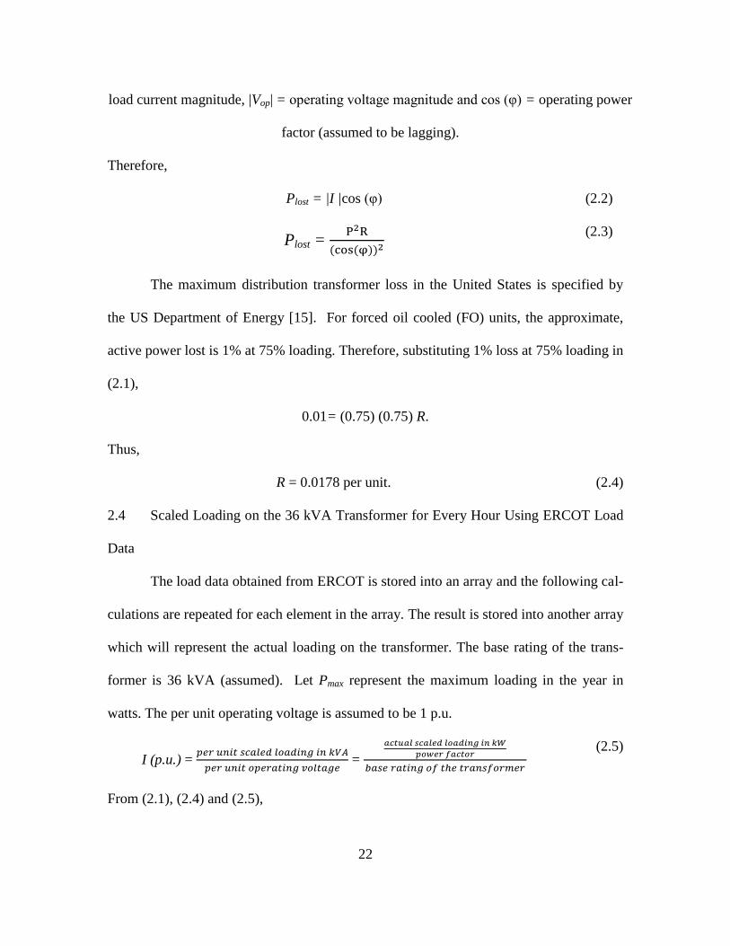
Figure 2.4 shows the assumed artifact distribution system. The total circuit rating
is 0.72 MVA which was selected to agree approximately with the original FREEDM de-
sign. Figure 2.4 shows 20 single phase distribution transformers each rated at 36 kVA,
8660/120 V. There are two principal types of electrical losses in conventional transform-
ers:
Core losses: these depend on the magnetic properties of materials used to con-
struct the core. Hysteresis loss and eddy current loss are the two types of core
losses in a transformer.
Copper losses: these vary depending on the loading of transformer.
Transformers are usually designed to utilize the core to the maximum. For pur-
poses of this study, core losses are neglected because full load and 75% full load opera-
tion is considered. This section evaluates losses in the 36 kVA conventional transformer
for the entire year of 2013 for different values of power factor- 60 %, 85 % and unity
power factor. The calculation of active power losses is shown as follows for a magnetic
transformer.
21
Figure 2.3 ERCOT Loading for the Year 2013 as Divided By Peak Load of the Year.
Figure 2.4 A Pictorial of a 0.72 MVA Feeder Showing 20 Distribution Transformers
Calculation of per unit resistance
The active power lost in a resistive element is,
Plost = R (2.1)
In per unit (p.u.), assuming |Vop| = 1 p.u., P =|Vop||I| cos (φ), where P = active power, |I| =
22
load current magnitude, |Vop| = operating voltage magnitude and cos (φ) = operating power
factor (assumed to be lagging).
Therefore,
Plost = |I |cos (φ) (2.2)
Plost =
(2.3)
The maximum distribution transformer loss in the United States is specified by
the US Department of Energy [15]. For forced oil cooled (FO) units, the approximate,
active power lost is 1% at 75% loading. Therefore, substituting 1% loss at 75% loading in
(2.1),
0.01= (0.75) (0.75) R.
Thus,
R = 0.0178 per unit. (2.4)
2.4 Scaled Loading on the 36 kVA Transformer for Every Hour Using ERCOT Load
Data
The load data obtained from ERCOT is stored into an array and the following cal-
culations are repeated for each element in the array. The result is stored into another array
which will represent the actual loading on the transformer. The base rating of the trans-
former is 36 kVA (assumed). Let Pmax represent the maximum loading in the year in
watts. The per unit operating voltage is assumed to be 1 p.u.
I (p.u.) =
=
(2.5)
From (2.1), (2.4) and (2.5),

23
I2R loss (p.u.) =|I|
2R (2.6)
I2R loss (actual) = I
2R loss (p.u.)*base rating of the transformer. (2.7)
The above calculations are carried out for each hour of the year and are summed
up to obtain the value of total energy lost per year in MWh/year.
2.5 Example Evaluation of Losses in a 36 kVA SST
This section evaluates losses in the 36 kVA SST for the entire year 2013. For es-
timating losses in an SST, 2 cases are considered:
A) 5% loss at 75% load.
B) 1% loss at 75% load.
Two types of losses are considered in the 36 kVA SST: switching losses and I2R
losses. For the sake of convenience, the switching losses are assumed to be 5 times the
I2R losses. Also, switching losses are proportional to the value of current flowing through
the transformer while the I2R losses are proportional to the square of the value of current
flowing through the transformer. Thus, the power loss formula has been approximately
formulated as follows:
Ploss = a |I| + b |I| 2, where a, b can be considered as loss coefficients (2.8)
The first term, a |I|, represents the switching loss and the second term, b |I| 2
rep-
resents the copper loss. Two cases are now shown to illustrate the model used in (2.8).
Two loss levels are illustrated.
Case A: Assuming 5% loss at 75% load
Ploss = a |I| + b |I|2.
In per unit,
24
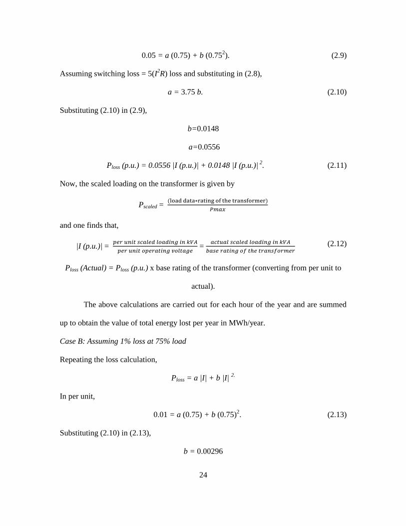
0.05 = a (0.75) + b (0.752). (2.9)
Assuming switching loss = 5(I2R) loss and substituting in (2.8),
a = 3.75 b. (2.10)
Substituting (2.10) in (2.9),
b=0.0148
a=0.0556
Ploss (p.u.) = 0.0556 |I (p.u.)| + 0.0148 |I (p.u.)| 2
. (2.11)
Now, the scaled loading on the transformer is given by
Pscaled =
and one finds that,
|I (p.u.)| =
=
(2.12)
Ploss (Actual) = Ploss (p.u.) x base rating of the transformer (converting from per unit to
actual).
The above calculations are carried out for each hour of the year and are summed
up to obtain the value of total energy lost per year in MWh/year.
Case B: Assuming 1% loss at 75% load
Repeating the loss calculation,
Ploss = a |I| + b |I| 2.
In per unit,
0.01 = a (0.75) + b (0.75)2. (2.13)
Substituting (2.10) in (2.13),
b = 0.00296
25
a = 0.01111
Ploss (p.u.) = 0.01111 |I (p.u.)| + 0.00296 |I (p.u.)| 2
. (2.14)
The scaled loading on the transformer is given by
=
From which one finds |I (p.u.)| from (2.12). Therefore,
Ploss (actual) = Ploss (p.u.) x base rating of the transformer (converting from per unit to
actual).
The above calculations are carried out for each hour of the year and are summed
up to obtain the value of total energy lost per year in MWh/year.
2.6 Annual Energy Loss for a 36 kVA Magnetic Transformer
The value of energy lost obtained in Section 2.4 is then multiplied with the aver-
age cost of energy to obtain the value of the cost of energy lost for the transformer for the
entire year in $/year. Average cost of energy is taken as 10.27 cents/kWh as obtained
from [14] for the year 2012. The MATLAB code used to obtain this value is attached in
the Appendix A. A summary of resulting calculations over a range of power factors is
presented in a subsequent summary section.
2.7 Annual Energy Loss: 36 kVA SST
The previous section related to magnetic transformer losses. In this section, the
same calculation is repeated for an SST. The value of energy lost obtained in Section 2.5
is then multiplied with the average cost of energy to obtain the value of the cost of energy
lost for the transformer for the entire year in $/year. Average cost of energy is taken as
10.27 cents/kWh as obtained from [14] for the year 2012. The MATLAB code used to
obtain this value is attached in the Appendix B. A summary of resulting calculations over
26
a range of power factors is presented in a subsequent summary section.
2.8 An Algorithm for Calculation of Annual Energy Loss in Transformers
Algorithms for the calculation of active power losses in a 36 kVA conventional
(magnetic) transformer and also for an SST are as follows:
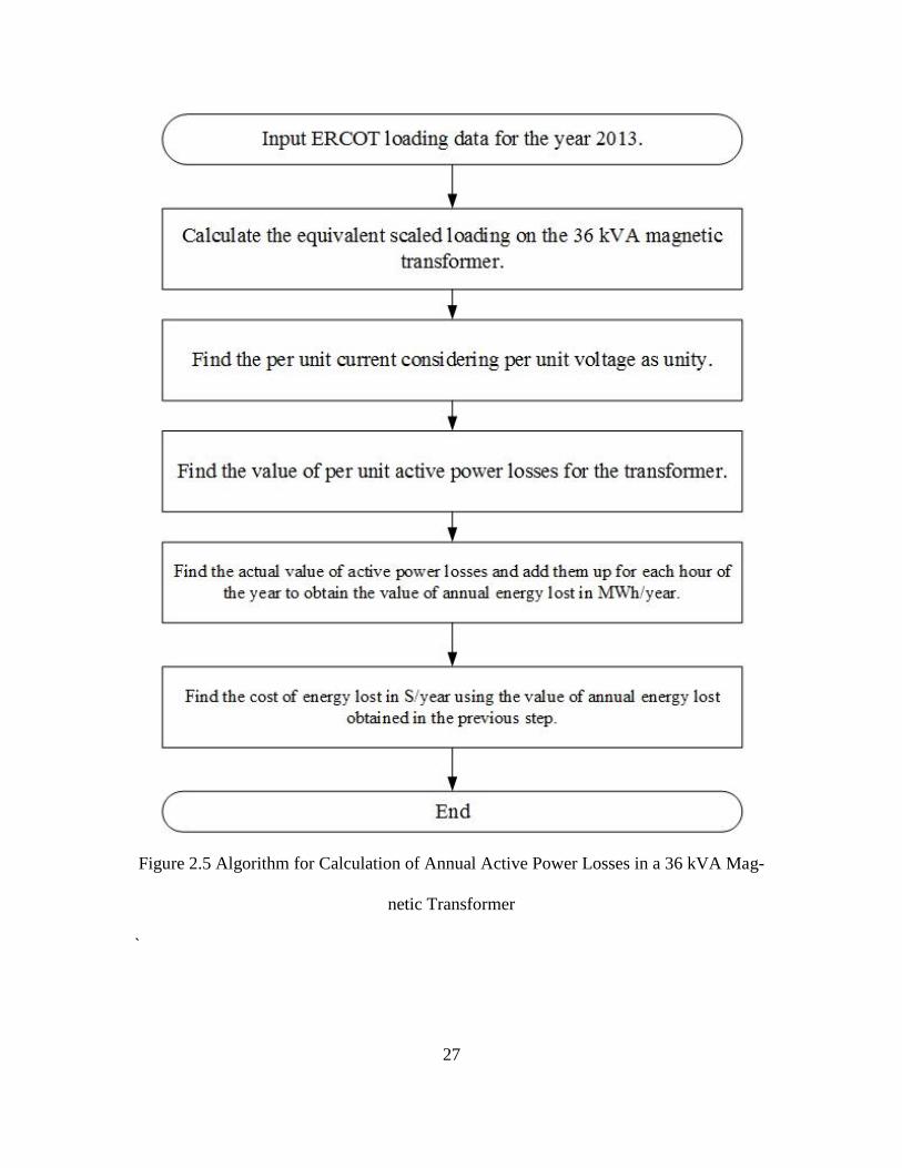
Algorithm for 36 kVA Magnetic transformer
Figure 2.5 shows a pictorial of the algorithm for the calculation of annual active
power losses in a 36 kVA magnetic transformer.
Algorithm for 36 kVA SST
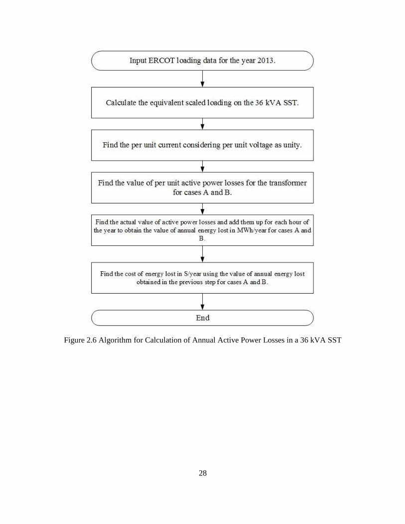
Figure 2.6 shows a pictorial of an algorithm for calculation of annual active power
losses in a 36 kVA SST. Figure 2.9 gives a summary of annual energy lost in a 36 kVA
SST. Figure 2.10 gives a summary of annual cost of energy lost in a 36 kVA magnetic
transformer.
2.9 Calculation Summary for Transformer Active Power Losses
In this section, the active power losses for both the magnetic and electronic trans-
former are summarized. Table 2.1 shows the results for losses in a conventional 36 kVA
transformer. Table 2.2 is a similar summary for an SST.
27
Figure 2.5 Algorithm for Calculation of Annual Active Power Losses in a 36 kVA Mag-
netic Transformer
`
28
Figure 2.6 Algorithm for Calculation of Annual Active Power Losses in a 36 kVA SST
29
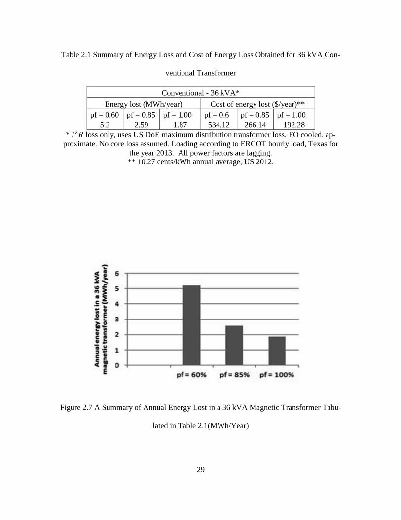
Table 2.1 Summary of Energy Loss and Cost of Energy Loss Obtained for 36 kVA Con-
ventional Transformer
Conventional - 36 kVA*
Energy lost (MWh/year) Cost of energy lost ($/year)**
pf = 0.60 pf = 0.85 pf = 1.00 pf = 0.6 pf = 0.85 pf = 1.00
5.2 2.59 1.87 534.12 266.14 192.28
* loss only, uses US DoE maximum distribution transformer loss, FO cooled, ap-
proximate. No core loss assumed. Loading according to ERCOT hourly load, Texas for
the year 2013. All power factors are lagging.
** 10.27 cents/kWh annual average, US 2012.
Figure 2.7 A Summary of Annual Energy Lost in a 36 kVA Magnetic Transformer Tabu-
lated in Table 2.1(MWh/Year)
30
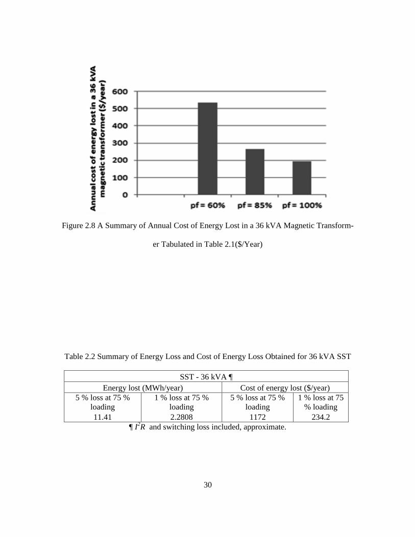
Figure 2.8 A Summary of Annual Cost of Energy Lost in a 36 kVA Magnetic Transform-
er Tabulated in Table 2.1($/Year)
Table 2.2 Summary of Energy Loss and Cost of Energy Loss Obtained for 36 kVA SST
SST - 36 kVA 
Energy lost (MWh/year) Cost of energy lost ($/year)
5 % loss at 75 %
loading
1 % loss at 75 %
loading
5 % loss at 75 %
loading
1 % loss at 75
% loading
11.41 2.2808 1172 234.2
¶ I2R and switching loss included, approximate.
31
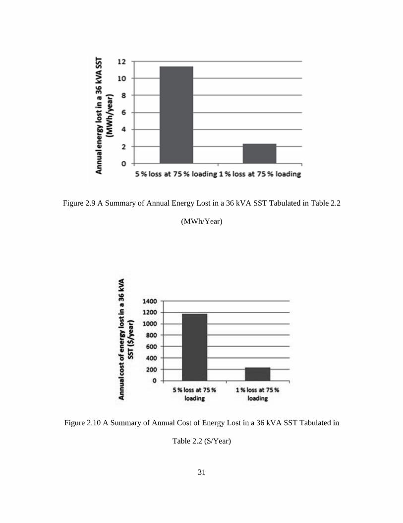
Figure 2.9 A Summary of Annual Energy Lost in a 36 kVA SST Tabulated in Table 2.2
(MWh/Year)
Figure 2.10 A Summary of Annual Cost of Energy Lost in a 36 kVA SST Tabulated in
Table 2.2 ($/Year)
32
CHAPTER 3 ACTIVE POWER LOSSES IN DISTRIBUTION PRIMARY CONDUC-
TORS
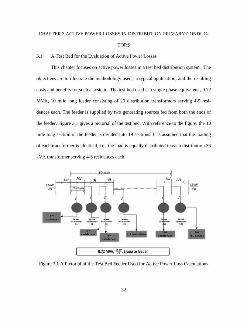
3.1 A Test Bed for the Evaluation of Active Power Losses
This chapter focuses on active power losses in a test bed distribution system. The
objectives are to illustrate the methodology used; a typical application; and the resulting
costs and benefits for such a system. The test bed used is a single phase equivalent , 0.72
MVA, 10 mile long feeder consisting of 20 distribution transformers serving 4-5 resi-
dences each. The feeder is supplied by two generating sources fed from both the ends of
the feeder. Figure 3.1 gives a pictorial of the test bed. With reference to the figure, the 10
mile long section of the feeder is divided into 19 sections. It is assumed that the loading
of each transformer is identical, i.e., the load is equally distributed in each distribution 36
kVA transformer serving 4-5 residences each.
Figure 3.1 A Pictorial of the Test Bed Feeder Used for Active Power Loss Calculations

33
From the ERCOT load data obtained, for every hour of the year 2013 [13], the
active power losses are calculated for each of the sections and are summed to obtain the
total active power lost in the feeder for that particular hour. In a similar manner, active
power lost in the feeder is calculated for every hour of the year 2013 and is summed to
obtain the annual total active power lost in the feeder. These calculations are done for two
cases: assuming that all the distribution level 36 kVA transformers are magnetic trans-
formers; and assuming that all the distribution level 36 kVA transformers are SSTs. The-
se calculations are then compared to identify in which case more active power losses are
incurred. For the magnetic transformer, three cases are considered: transformer operating
at 60% power factor lagging; transformer operating at 85% power factor lagging; and
transformer operating at unity power factor. These use cases span the typical range of
power factor of residential loads.
3.2 Example Evaluation of Feeder Losses with 36 kVA Magnetic Transformers
For the feeder shown in Figure 3.1, #2 Aluminum conductors are assumed. For
this conductor, the resistance is 1.41 Ω/mile [16]. The 10 mile long section of the feeder
is divided into 19 sections of equal length as seen in Figure 3.1. Each section starts and
ends with a 36 kVA distribution transformer.
Base rating of the transformer = 36 kVA (assumed)
Pmax represents the maximum loading in the year in watts
The operating voltage is given by
.
The load data are obtained from ERCOT loading data for the year 2013. These
data give the load in MW for every hour of the year 2013. Thus, 8760 values of scaled
loading on the 36 kVA transformer are obtained as follows:
34
|I| =
=
.
(3.1)
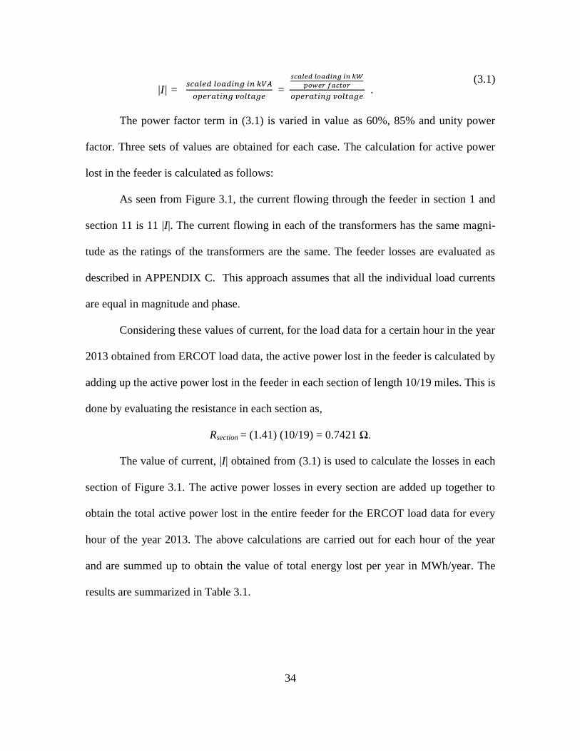
The power factor term in (3.1) is varied in value as 60%, 85% and unity power
factor. Three sets of values are obtained for each case. The calculation for active power
lost in the feeder is calculated as follows:
As seen from Figure 3.1, the current flowing through the feeder in section 1 and
section 11 is 11 |I|. The current flowing in each of the transformers has the same magni-
tude as the ratings of the transformers are the same. The feeder losses are evaluated as
described in APPENDIX C. This approach assumes that all the individual load currents
are equal in magnitude and phase.
Considering these values of current, for the load data for a certain hour in the year
2013 obtained from ERCOT load data, the active power lost in the feeder is calculated by
adding up the active power lost in the feeder in each section of length 10/19 miles. This is
done by evaluating the resistance in each section as,
Rsection = (1.41) (10/19) = 0.7421 Ω.
The value of current, |I| obtained from (3.1) is used to calculate the losses in each
section of Figure 3.1. The active power losses in every section are added up together to
obtain the total active power lost in the entire feeder for the ERCOT load data for every
hour of the year 2013. The above calculations are carried out for each hour of the year
and are summed up to obtain the value of total energy lost per year in MWh/year. The
results are summarized in Table 3.1.
35
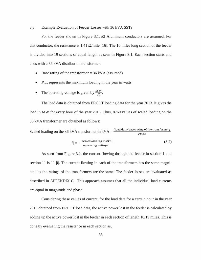
3.3 Example Evaluation of Feeder Losses with 36 kVA SSTs
For the feeder shown in Figure 3.1, #2 Aluminum conductors are assumed. For
this conductor, the resistance is 1.41 Ω/mile [16]. The 10 miles long section of the feeder
is divided into 19 sections of equal length as seen in Figure 3.1. Each section starts and
ends with a 36 kVA distribution transformer.
Base rating of the transformer = 36 kVA (assumed)
Pmax represents the maximum loading in the year in watts.
The operating voltage is given by
.
The load data is obtained from ERCOT loading data for the year 2013. It gives the
load in MW for every hour of the year 2013. Thus, 8760 values of scaled loading on the
36 kVA transformer are obtained as follows:
Scaled loading on the 36 kVA transformer in kVA =
|I| =
. (3.2)
As seen from Figure 3.1, the current flowing through the feeder in section 1 and
section 11 is 11 |I|. The current flowing in each of the transformers has the same magni-
tude as the ratings of the transformers are the same. The feeder losses are evaluated as
described in APPENDIX C. This approach assumes that all the individual load currents
are equal in magnitude and phase.
Considering these values of current, for the load data for a certain hour in the year
2013 obtained from ERCOT load data, the active power lost in the feeder is calculated by
adding up the active power lost in the feeder in each section of length 10/19 miles. This is
done by evaluating the resistance in each section as,
36
Rsection = (1.41)(10/19) = 0.7421 Ω.
The value of current, |I| obtained from (3.2) is used to calculate the losses in each
section of Figure 3.1. The active power losses in every section are added up together to
obtain the total active power lost in the entire feeder for the ERCOT load data for every
hour of the year 2013. The above calculations are carried out for each hour of the year
and are summed up to obtain the value of total energy lost per year in MWh/year. The
results are summarized in Table 3.1.
3.4 Annual Energy Loss in Feeder: Using 36 kVA Magnetic Transformers
The value of energy lost obtained in Section 3.2 is then multiplied with the aver-
age cost of energy to obtain the value of the cost of energy lost in the feeder using 20 dis-
tribution level magnetic transformers for the entire year in $/year. Average cost of energy
is taken as 10.27 cents/kWh as obtained from [14]. The MATLAB code used to obtain
this value is attached in the Appendix C section. It assumes that the system is operating at
unity power factor. The value of power factor is modified to obtain results for 60 % and
85 % power factor cases.
3.5 Annual Energy Loss in Feeder: Using 36 kVA SSTs
The value of energy lost obtained in Section 3.2 is then multiplied with the aver-
age cost of energy to obtain the value of the energy lost in the feeder. The assumption is
that 20 distribution level SSTs operate for the entire year. The cost is in $/year. Average
cost of energy is taken as 10.27 cents/kWh as obtained from [14]. The MATLAB code
used to obtain this value is attached in the Appendix C section.
37
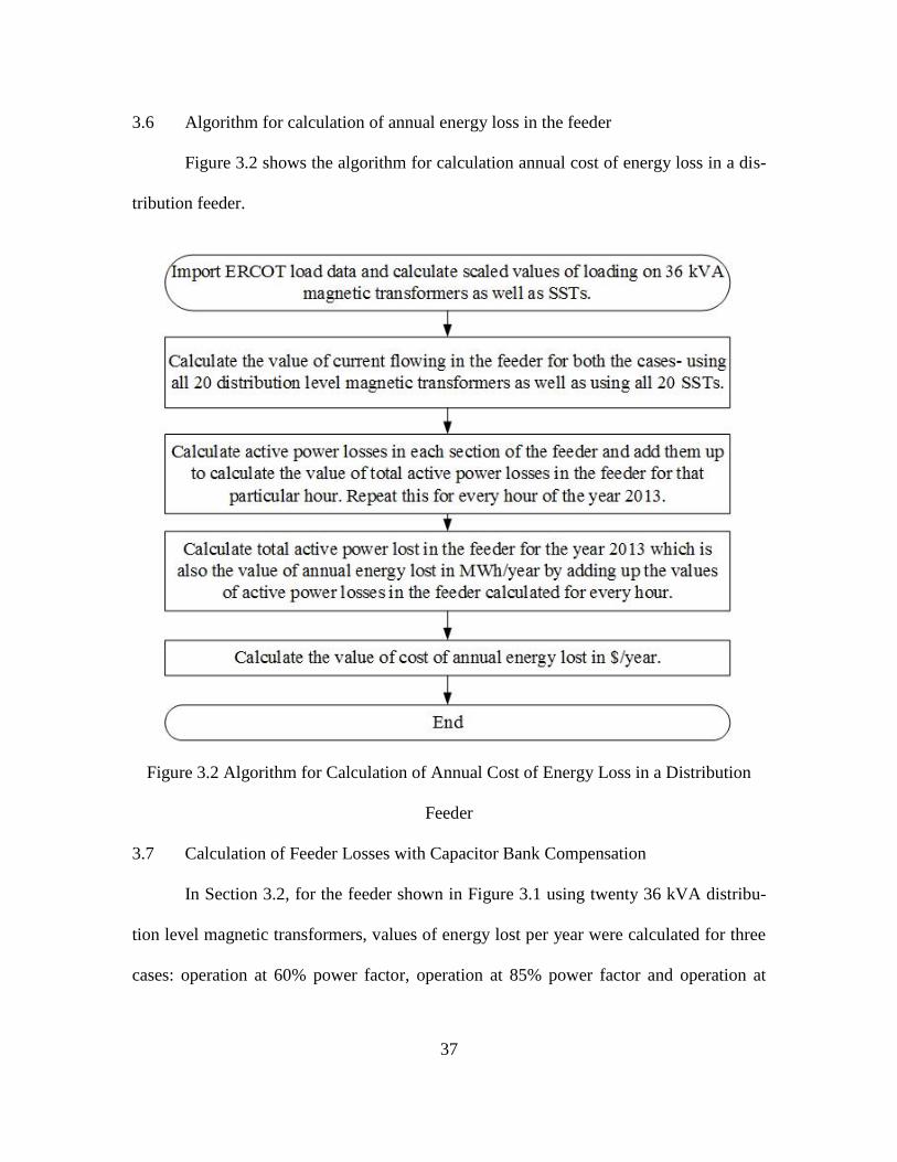
3.6 Algorithm for calculation of annual energy loss in the feeder
Figure 3.2 shows the algorithm for calculation annual cost of energy loss in a dis-
tribution feeder.
Figure 3.2 Algorithm for Calculation of Annual Cost of Energy Loss in a Distribution
Feeder
3.7 Calculation of Feeder Losses with Capacitor Bank Compensation
In Section 3.2, for the feeder shown in Figure 3.1 using twenty 36 kVA distribu-
tion level magnetic transformers, values of energy lost per year were calculated for three
cases: operation at 60% power factor, operation at 85% power factor and operation at

38
unity power factor. Capacitor banks were introduced to improve the power factor as fol-
lows:
Case 1: Improve power factor from 60% to 85%.
For this case, the transformers will continue to operate at 60% power factor while
the distribution lines will be operating at 85% power factor and the value of energy lost
per year in the feeder in this case will be equivalent to the case when the system incurs
losses at 85% power factor. The system will incur lesser losses as compared to the 60%
power factor case due to reduction in the current flowing through the lines at 85% power
factor. But this reduction in the cost of energy lost per year will also be accompanied by
an increase in cost of installing additional capacitor banks.
Case 2: Improve power factor from 85% to 100%.
For this case, the transformers will continue to operate at 85% power factor while
the distribution lines will be operating at 100% power factor and the value of energy lost
per year in the feeder in this case will be equivalent to the case when the system incurs
losses at 100% power factor. The system will incur lesser losses as compared to the 85%
power factor case due to reduction in the current flowing through the lines at 100% pow-
er factor. But this reduction in the cost of energy lost per year will also be accompanied
by an increase in cost of installing additional capacitor banks.
Case 3: Improve power factor from 60% to 100%.
For this case, the transformers will continue to operate at 60% power factor while
the distribution lines will be operating at 100% power factor and the value of energy lost
per year in the feeder in this case will be equivalent to the case when the system incurs
losses at 100% power factor. The system will incur lesser losses as compared to the 60%
39
power factor case due to reduction in the current flowing through the lines at 100% pow-
er factor. But this reduction in the cost of energy lost per year will also be accompanied
by an increase in cost of installing additional capacitor banks. These values are tabulated
in Table 3.1.
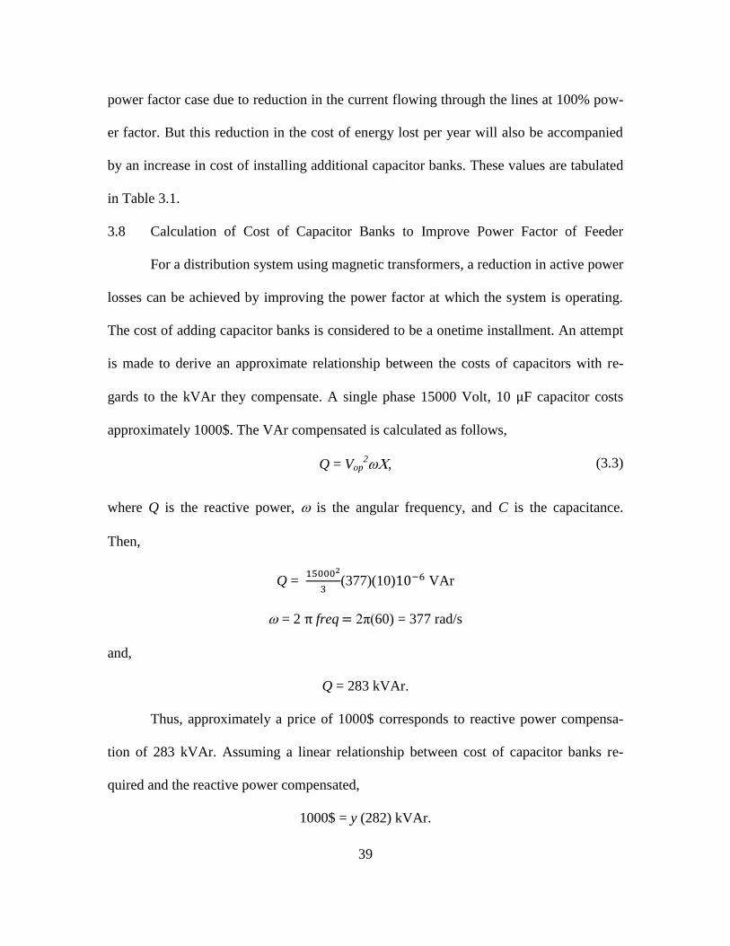
3.8 Calculation of Cost of Capacitor Banks to Improve Power Factor of Feeder
For a distribution system using magnetic transformers, a reduction in active power
losses can be achieved by improving the power factor at which the system is operating.
The cost of adding capacitor banks is considered to be a onetime installment. An attempt
is made to derive an approximate relationship between the costs of capacitors with re-
gards to the kVAr they compensate. A single phase 15000 Volt, 10 F capacitor costs
approximately 1000$. The VAr compensated is calculated as follows,
Q = Vop2, (3.3)
where Q is the reactive power, is the angular frequency, and C is the capacitance.
Then,
Q =
(377)(10) VAr
= 2 π freq 2π(60) = 377 rad/s
and,
Q = 283 kVAr.
Thus, approximately a price of 1000$ corresponds to reactive power compensa-
tion of 283 kVAr. Assuming a linear relationship between cost of capacitor banks re-
quired and the reactive power compensated,
1000$ = y (282) kVAr.
40
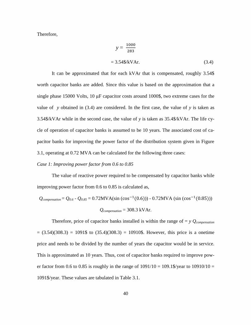
Therefore,
y =
= 3.54$/kVAr. (3.4)
It can be approximated that for each kVAr that is compensated, roughly 3.54$
worth capacitor banks are added. Since this value is based on the approximation that a
single phase 15000 Volts, 10 F capacitor costs around 1000$, two extreme cases for the
value of y obtained in (3.4) are considered. In the first case, the value of y is taken as
3.54$/kVAr while in the second case, the value of y is taken as 35.4$/kVAr. The life cy-
cle of operation of capacitor banks is assumed to be 10 years. The associated cost of ca-
pacitor banks for improving the power factor of the distribution system given in Figure
3.1, operating at 0.72 MVA can be calculated for the following three cases:
Case 1: Improving power factor from 0.6 to 0.85
The value of reactive power required to be compensated by capacitor banks while
improving power factor from 0.6 to 0.85 is calculated as,
Qcompensation = Q0.6 - Q0.85 = 0.72MVA(sin ( )) - 0.72MVA (sin ( ))
Qcompensation = 308.3 kVAr.
Therefore, price of capacitor banks installed is within the range of = y Qcompensation
= (3.54)(308.3) = 1091$ to (35.4)(308.3) = 10910$. However, this price is a onetime
price and needs to be divided by the number of years the capacitor would be in service.
This is approximated as 10 years. Thus, cost of capacitor banks required to improve pow-
er factor from 0.6 to 0.85 is roughly in the range of 1091/10 = 109.1$/year to 10910/10 =
1091$/year. These values are tabulated in Table 3.1.
41
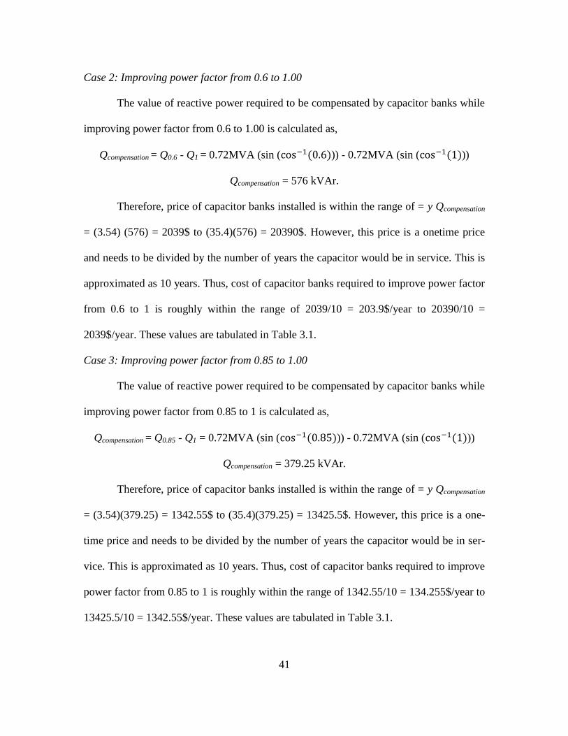
Case 2: Improving power factor from 0.6 to 1.00
The value of reactive power required to be compensated by capacitor banks while
improving power factor from 0.6 to 1.00 is calculated as,
Qcompensation = Q0.6 - Q1 = 0.72MVA (sin ( )) - 0.72MVA (sin ( ))
Qcompensation = 576 kVAr.
Therefore, price of capacitor banks installed is within the range of = y Qcompensation
= (3.54) (576) = 2039$ to (35.4)(576) = 20390$. However, this price is a onetime price
and needs to be divided by the number of years the capacitor would be in service. This is
approximated as 10 years. Thus, cost of capacitor banks required to improve power factor
from 0.6 to 1 is roughly within the range of 2039/10 = 203.9$/year to 20390/10 =
2039$/year. These values are tabulated in Table 3.1.
Case 3: Improving power factor from 0.85 to 1.00
The value of reactive power required to be compensated by capacitor banks while
improving power factor from 0.85 to 1 is calculated as,
Qcompensation = Q0.85 - Q1 = 0.72MVA (sin ( )) - 0.72MVA (sin ( ))
Qcompensation = 379.25 kVAr.
Therefore, price of capacitor banks installed is within the range of = y Qcompensation
= (3.54)(379.25) = 1342.55$ to (35.4)(379.25) = 13425.5$. However, this price is a one-
time price and needs to be divided by the number of years the capacitor would be in ser-
vice. This is approximated as 10 years. Thus, cost of capacitor banks required to improve
power factor from 0.85 to 1 is roughly within the range of 1342.55/10 = 134.255$/year to
13425.5/10 = 1342.55$/year. These values are tabulated in Table 3.1.
42
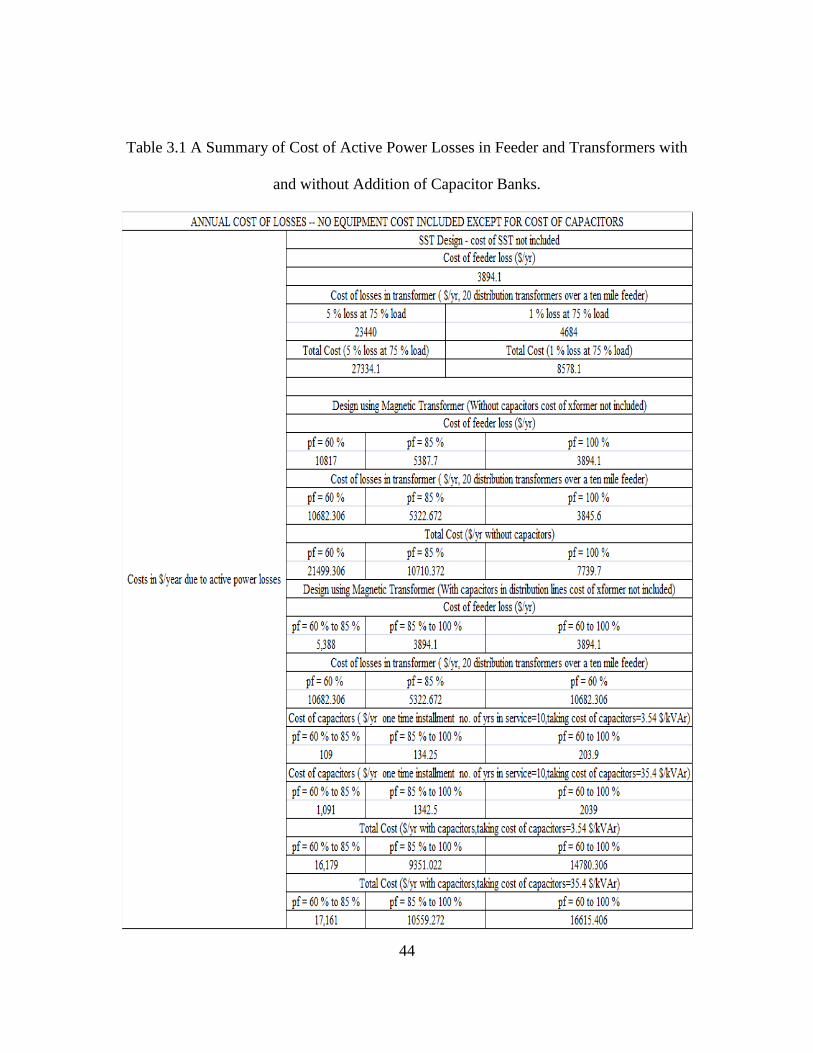
3.9 Calculation Summary of Line and Transformer Active Power Losses
Table 3.1 excludes cost of transformers. For an SST, typical cost of the trans-
former after technology matures can be estimated at around 67$/ kVA for a single phase
unit [20]. Thus, a single 36 kVA SST will cost around 67*36 = 2,412$ after technology
matures. As per [5], the ratio of cost of a 1 MVA SST to that of a magnetic transformer
of the same rating is predicted to be 4.61. The average life expectancy of a medium volt-
age distribution level 36 kVA SST can be assumed to be 12 years while that of a magnet-
ic transformer of the same rating can be assumed to be 20 years.
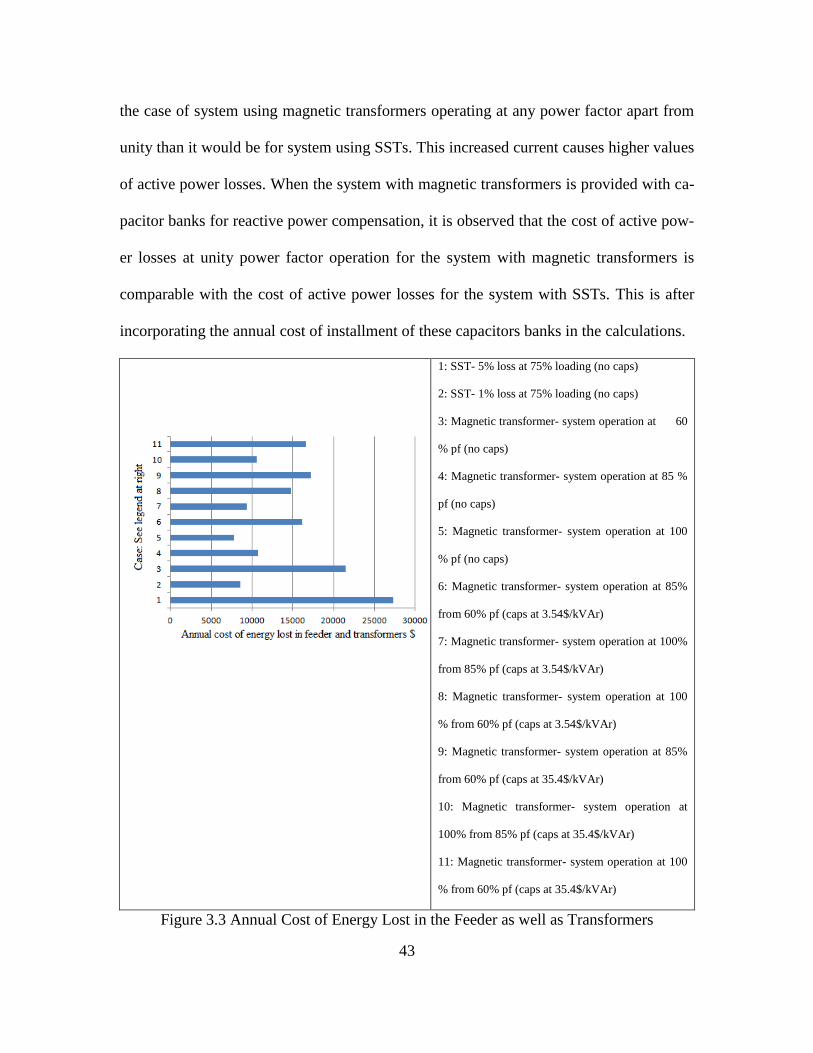
3.10 Summary of Results
The annual cost of active power losses in the 20 transformers as well as the distri-
bution feeder for the system shown in Figure 3.1 are tabulated in Table 3.1 for both the
cases: system having solid state transformers and system having magnetic transformers.
This is done for the ERCOT load data for the year 2013 [13]. For the magnetic trans-
former case, operation at three different power factors is considered: 60%, 85% and unity
power factor. Capacitor bank compensation is also provided to improve the power factor
from 60% to 85%, 85% to 100% and 60% to 100%. The results obtained for these cases
are summarized in Figure 3.3.
The feeder loss for the case with all SSTs is the same as the case with magnetic
transformers operating at 100% power factor. This is because the current flowing in the
system with SSTs would be the same as the current flowing in the system with magnetic
transformers operating at unity power factor. The system incurs high losses in the mag-
netic transformer case for power factor operation at 60 % and 85%. as compared to the
SST case. This is because, the current flowing in the feeder and transformers is higher in
43
the case of system using magnetic transformers operating at any power factor apart from
unity than it would be for system using SSTs. This increased current causes higher values
of active power losses. When the system with magnetic transformers is provided with ca-
pacitor banks for reactive power compensation, it is observed that the cost of active pow-
er losses at unity power factor operation for the system with magnetic transformers is
comparable with the cost of active power losses for the system with SSTs. This is after
incorporating the annual cost of installment of these capacitors banks in the calculations.
1: SST- 5% loss at 75% loading (no caps)
2: SST- 1% loss at 75% loading (no caps)
3: Magnetic transformer- system operation at 60
% pf (no caps)
4: Magnetic transformer- system operation at 85 %
pf (no caps)
5: Magnetic transformer- system operation at 100
% pf (no caps)
6: Magnetic transformer- system operation at 85%
from 60% pf (caps at 3.54$/kVAr)
7: Magnetic transformer- system operation at 100%
from 85% pf (caps at 3.54$/kVAr)
8: Magnetic transformer- system operation at 100
% from 60% pf (caps at 3.54$/kVAr)
9: Magnetic transformer- system operation at 85%
from 60% pf (caps at 35.4$/kVAr)
10: Magnetic transformer- system operation at
100% from 85% pf (caps at 35.4$/kVAr)
11: Magnetic transformer- system operation at 100
% from 60% pf (caps at 35.4$/kVAr)
Figure 3.3 Annual Cost of Energy Lost in the Feeder as well as Transformers
44
Table 3.1 A Summary of Cost of Active Power Losses in Feeder and Transformers with
and without Addition of Capacitor Banks.
45
CHAPTER 4 RELIABILITY OF SERVICE TO CUSTOMERS AND NUMBER OF
FIDs
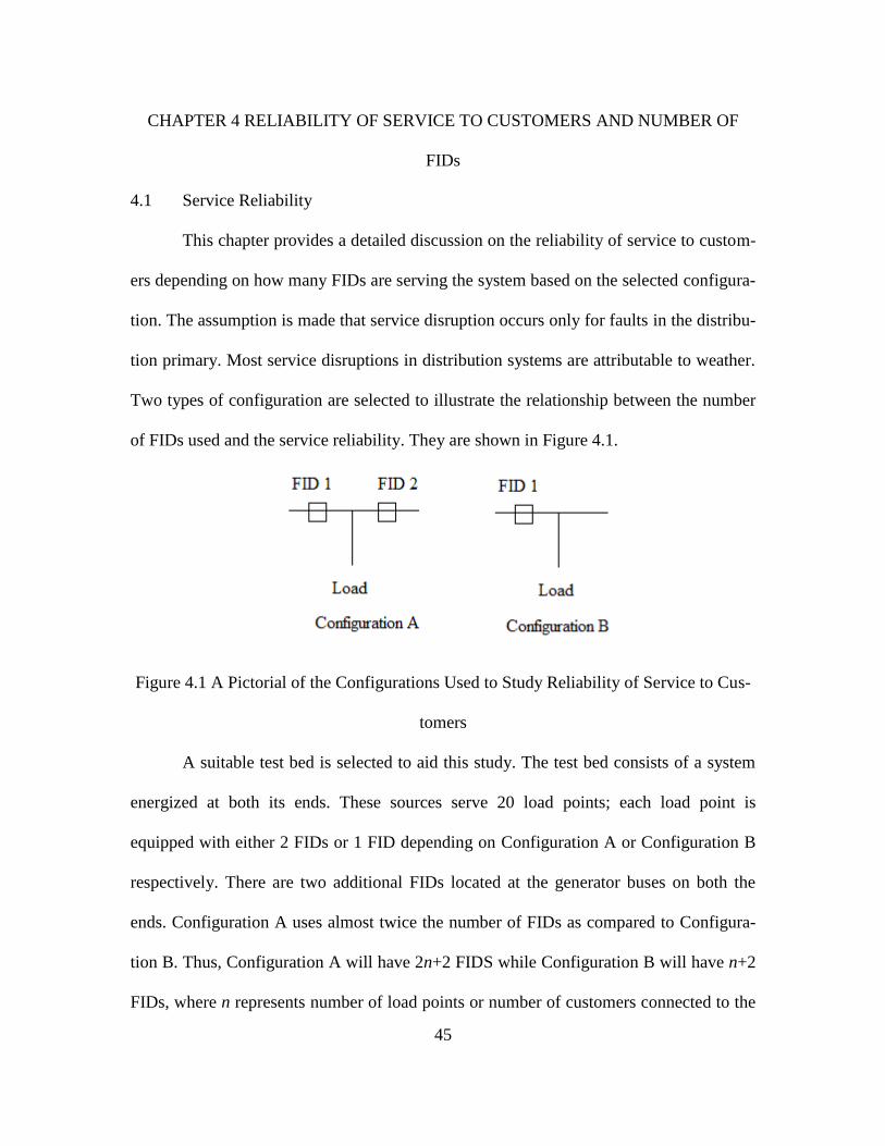
4.1 Service Reliability
This chapter provides a detailed discussion on the reliability of service to custom-
ers depending on how many FIDs are serving the system based on the selected configura-
tion. The assumption is made that service disruption occurs only for faults in the distribu-
tion primary. Most service disruptions in distribution systems are attributable to weather.
Two types of configuration are selected to illustrate the relationship between the number
of FIDs used and the service reliability. They are shown in Figure 4.1.
Figure 4.1 A Pictorial of the Configurations Used to Study Reliability of Service to Cus-
tomers
A suitable test bed is selected to aid this study. The test bed consists of a system
energized at both its ends. These sources serve 20 load points; each load point is
equipped with either 2 FIDs or 1 FID depending on Configuration A or Configuration B
respectively. There are two additional FIDs located at the generator buses on both the
ends. Configuration A uses almost twice the number of FIDs as compared to Configura-
tion B. Thus, Configuration A will have 2n+2 FIDS while Configuration B will have n+2
FIDs, where n represents number of load points or number of customers connected to the
46
service.
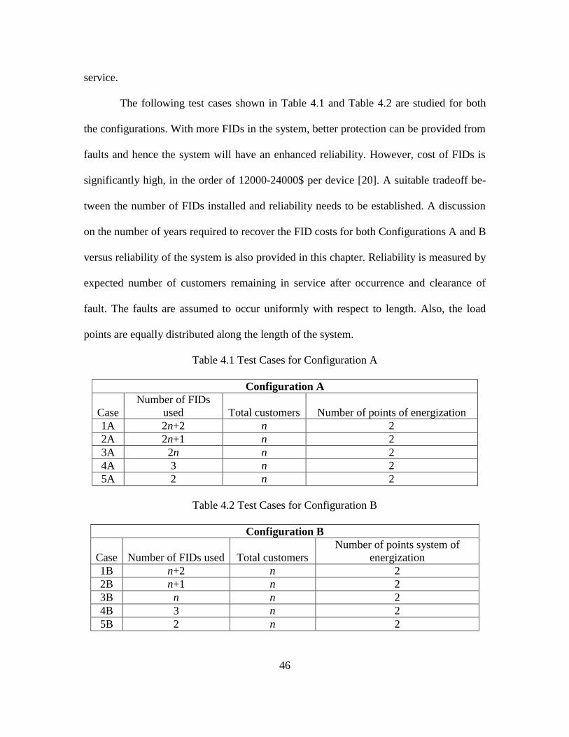
The following test cases shown in Table 4.1 and Table 4.2 are studied for both
the configurations. With more FIDs in the system, better protection can be provided from
faults and hence the system will have an enhanced reliability. However, cost of FIDs is
significantly high, in the order of 12000-24000$ per device [20]. A suitable tradeoff be-
tween the number of FIDs installed and reliability needs to be established. A discussion
on the number of years required to recover the FID costs for both Configurations A and B
versus reliability of the system is also provided in this chapter. Reliability is measured by
expected number of customers remaining in service after occurrence and clearance of
fault. The faults are assumed to occur uniformly with respect to length. Also, the load
points are equally distributed along the length of the system.
Table 4.1 Test Cases for Configuration A
Configuration A
Case
Number of FIDs
used Total customers Number of points of energization
1A 2n+2 n 2
2A 2n+1 n 2
3A 2n n 2
4A 3 n 2
5A 2 n 2
Table 4.2 Test Cases for Configuration B
Configuration B
Case Number of FIDs used Total customers
Number of points system of
energization
1B n+2 n 2
2B n+1 n 2
3B n n 2
4B 3 n 2
5B 2 n 2
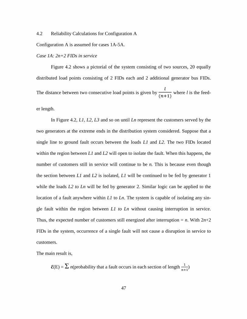
47
4.2 Reliability Calculations for Configuration A
Configuration A is assumed for cases 1A-5A.
Case 1A: 2n+2 FIDs in service
Figure 4.2 shows a pictorial of the system consisting of two sources, 20 equally
distributed load points consisting of 2 FIDs each and 2 additional generator bus FIDs.
The distance between two consecutive load points is given by
where l is the feed-
er length.
In Figure 4.2, L1, L2, L3 and so on until Ln represent the customers served by the
two generators at the extreme ends in the distribution system considered. Suppose that a
single line to ground fault occurs between the loads L1 and L2. The two FIDs located
within the region between L1 and L2 will open to isolate the fault. When this happens, the
number of customers still in service will continue to be n. This is because even though
the section between L1 and L2 is isolated, L1 will be continued to be fed by generator 1
while the loads L2 to Ln will be fed by generator 2. Similar logic can be applied to the
location of a fault anywhere within L1 to Ln. The system is capable of isolating any sin-
gle fault within the region between L1 to Ln without causing interruption in service.
Thus, the expected number of customers still energized after interruption = n. With 2n+2
FIDs in the system, occurrence of a single fault will not cause a disruption in service to
customers.
The main result is,
E(E) = Σ n(probability that a fault occurs in each section of length
)
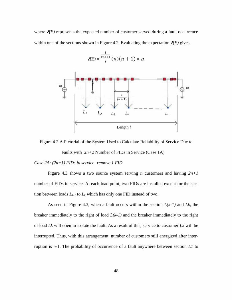
48
where E(E) represents the expected number of customer served during a fault occurrence
within one of the sections shown in Figure 4.2. Evaluating the expectation E(E) gives,
E(E) =
= n.
Figure 4.2 A Pictorial of the System Used to Calculate Reliability of Service Due to
Faults with 2n+2 Number of FIDs in Service (Case 1A)
Case 2A: (2n+1) FIDs in service- remove 1 FID
Figure 4.3 shows a two source system serving n customers and having 2n+1
number of FIDs in service. At each load point, two FIDs are installed except for the sec-
tion between loads Lk-1 to Lk which has only one FID instead of two.
As seen in Figure 4.3, when a fault occurs within the section L(k-1) and Lk, the
breaker immediately to the right of load L(k-1) and the breaker immediately to the right
of load Lk will open to isolate the fault. As a result of this, service to customer Lk will be
interrupted. Thus, with this arrangement, number of customers still energized after inter-
ruption is n-1. The probability of occurrence of a fault anywhere between section L1 to
L1 L2 L3 L4 Ln
Length l
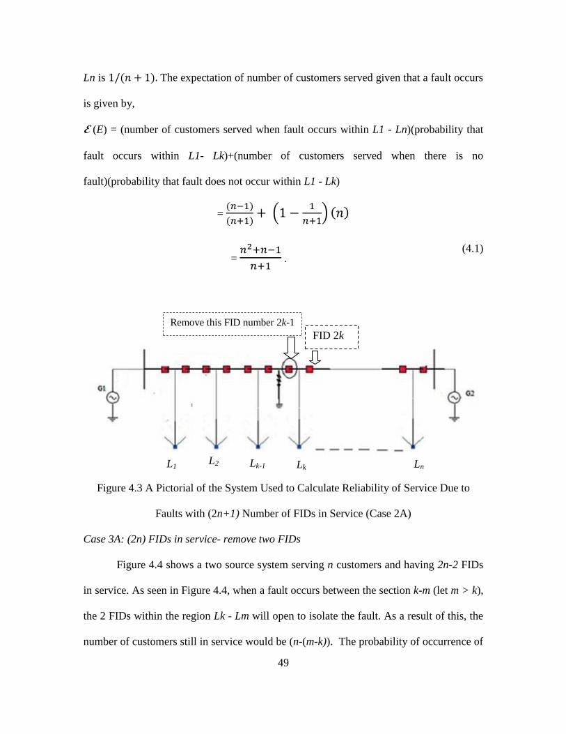
49
Ln is The expectation of number of customers served given that a fault occurs
is given by,
E (E) = (number of customers served when fault occurs within L1 - Ln)(probability that
fault occurs within L1- Lk)+(number of customers served when there is no
fault)(probability that fault does not occur within L1 - Lk)
=
=
.
(4.1)
Figure 4.3 A Pictorial of the System Used to Calculate Reliability of Service Due to
Faults with (2n+1) Number of FIDs in Service (Case 2A)
Case 3A: (2n) FIDs in service- remove two FIDs
Figure 4.4 shows a two source system serving n customers and having 2n-2 FIDs
in service. As seen in Figure 4.4, when a fault occurs between the section k-m (let m > k),
the 2 FIDs within the region Lk - Lm will open to isolate the fault. As a result of this, the
number of customers still in service would be (n-(m-k)). The probability of occurrence of
L1 L2 Lk-1 Lk Ln
Remove this FID number 2k-1
FID 2k
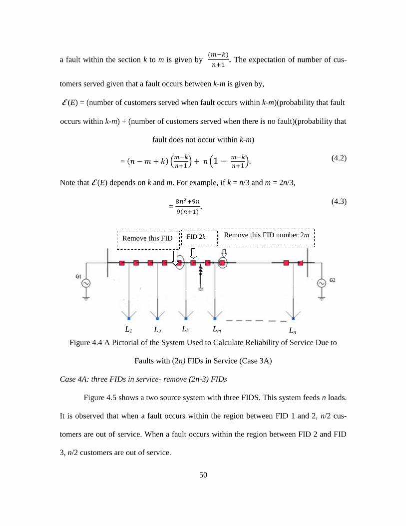
50
a fault within the section k to m is given by
. The expectation of number of cus-
tomers served given that a fault occurs between k-m is given by,
E (E) = (number of customers served when fault occurs within k-m)(probability that fault
occurs within k-m) + (number of customers served when there is no fault)(probability that
fault does not occur within k-m)
=
(4.2)
Note that E (E) depends on k and m. For example, if k = n/3 and m = 2n/3,
=
.
(4.3)
Figure 4.4 A Pictorial of the System Used to Calculate Reliability of Service Due to
Faults with (2n) FIDs in Service (Case 3A)
Case 4A: three FIDs in service- remove (2n-3) FIDs
Figure 4.5 shows a two source system with three FIDS. This system feeds n loads.
It is observed that when a fault occurs within the region between FID 1 and 2, n/2 cus-
tomers are out of service. When a fault occurs within the region between FID 2 and FID
3, n/2 customers are out of service.
L1 L2 Lk Lm Ln
Remove this FID number 2m FID 2k Remove this FID
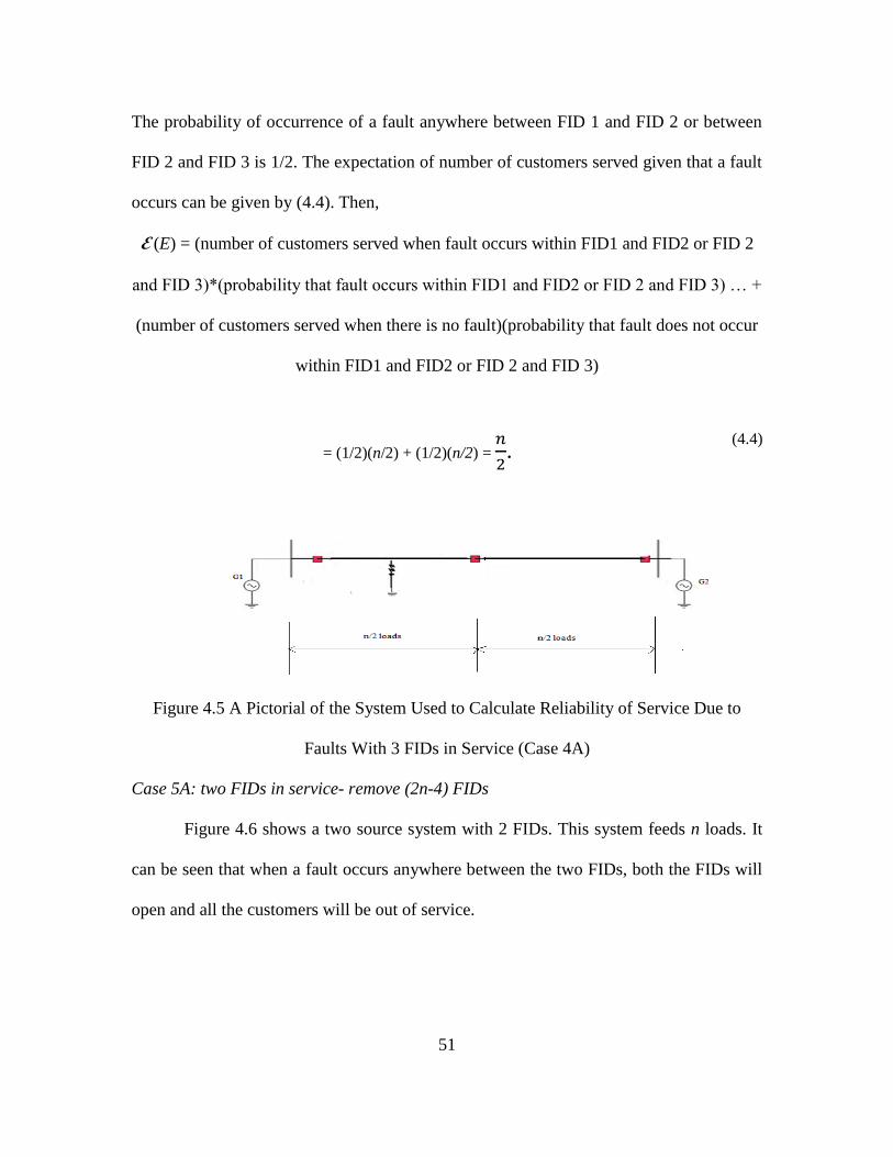
51
The probability of occurrence of a fault anywhere between FID 1 and FID 2 or between
FID 2 and FID 3 is 1/2. The expectation of number of customers served given that a fault
occurs can be given by (4.4). Then,
E (E) = (number of customers served when fault occurs within FID1 and FID2 or FID 2
and FID 3)*(probability that fault occurs within FID1 and FID2 or FID 2 and FID 3) … +
(number of customers served when there is no fault)(probability that fault does not occur
within FID1 and FID2 or FID 2 and FID 3)
= (1/2)(n/2) + (1/2)(n/2) =
.
(4.4)
Figure 4.5 A Pictorial of the System Used to Calculate Reliability of Service Due to
Faults With 3 FIDs in Service (Case 4A)
Case 5A: two FIDs in service- remove (2n-4) FIDs
Figure 4.6 shows a two source system with 2 FIDs. This system feeds n loads. It
can be seen that when a fault occurs anywhere between the two FIDs, both the FIDs will
open and all the customers will be out of service.
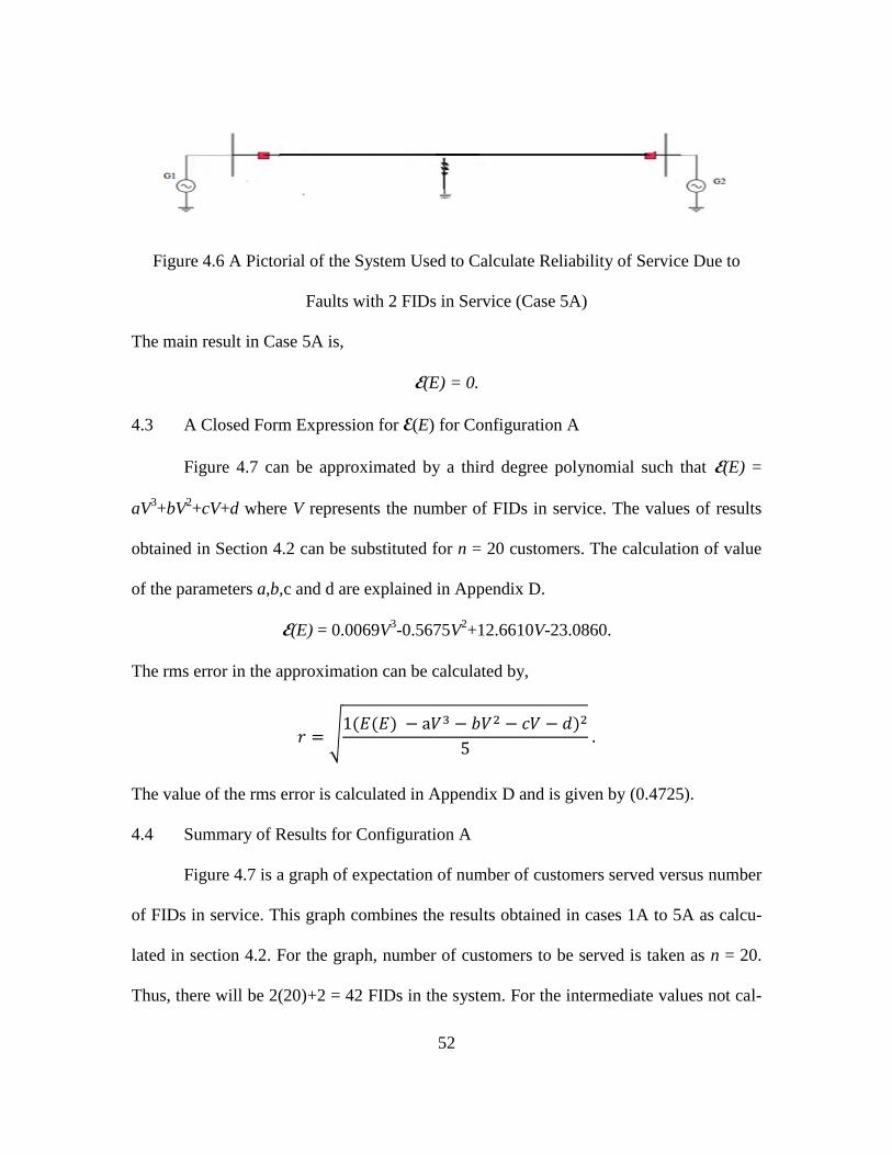
52
Figure 4.6 A Pictorial of the System Used to Calculate Reliability of Service Due to
Faults with 2 FIDs in Service (Case 5A)
The main result in Case 5A is,
E(E) = 0.
4.3 A Closed Form Expression for E(E) for Configuration A
Figure 4.7 can be approximated by a third degree polynomial such that E(E) =
aV3+bV
2+cV+d where V represents the number of FIDs in service. The values of results
obtained in Section 4.2 can be substituted for n = 20 customers. The calculation of value
of the parameters a,b,c and d are explained in Appendix D.
E(E) = 0.0069V3-0.5675V
2+12.6610V-23.0860.
The rms error in the approximation can be calculated by,
The value of the rms error is calculated in Appendix D and is given by (0.4725).
4.4 Summary of Results for Configuration A
Figure 4.7 is a graph of expectation of number of customers served versus number
of FIDs in service. This graph combines the results obtained in cases 1A to 5A as calcu-
lated in section 4.2. For the graph, number of customers to be served is taken as n = 20.
Thus, there will be 2(20)+2 = 42 FIDs in the system. For the intermediate values not cal-
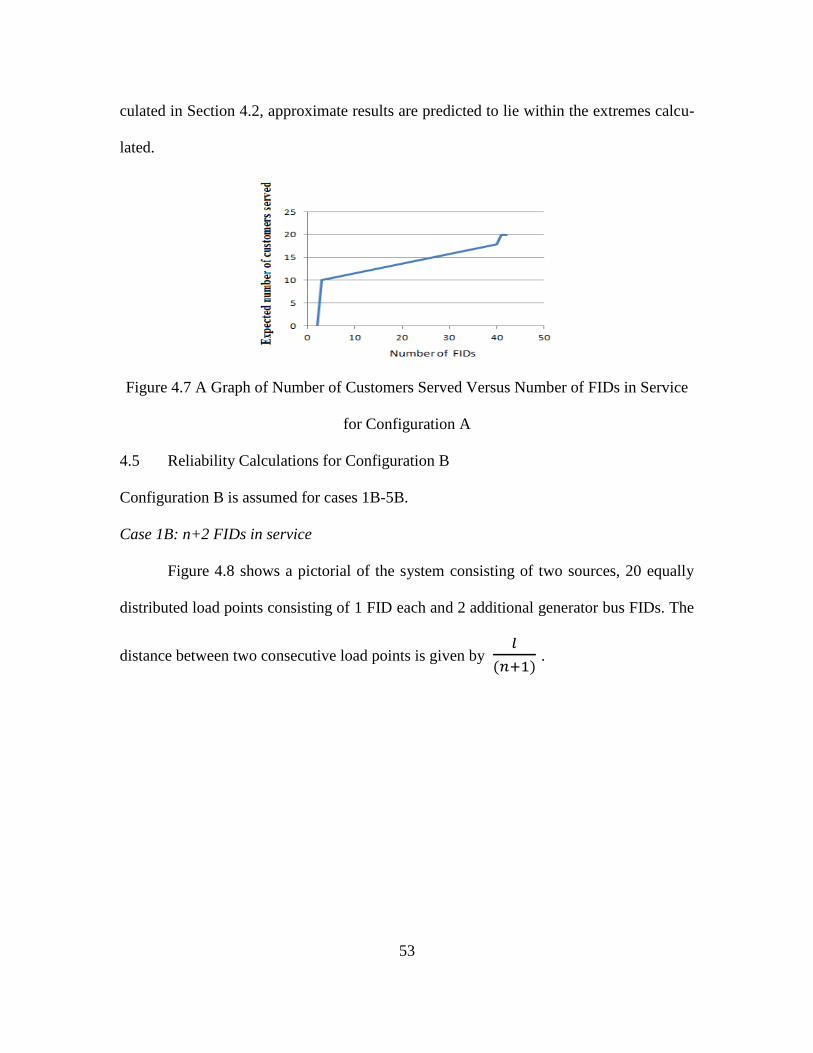
53
culated in Section 4.2, approximate results are predicted to lie within the extremes calcu-
lated.
Figure 4.7 A Graph of Number of Customers Served Versus Number of FIDs in Service
for Configuration A
4.5 Reliability Calculations for Configuration B
Configuration B is assumed for cases 1B-5B.
Case 1B: n+2 FIDs in service
Figure 4.8 shows a pictorial of the system consisting of two sources, 20 equally
distributed load points consisting of 1 FID each and 2 additional generator bus FIDs. The
distance between two consecutive load points is given by
.
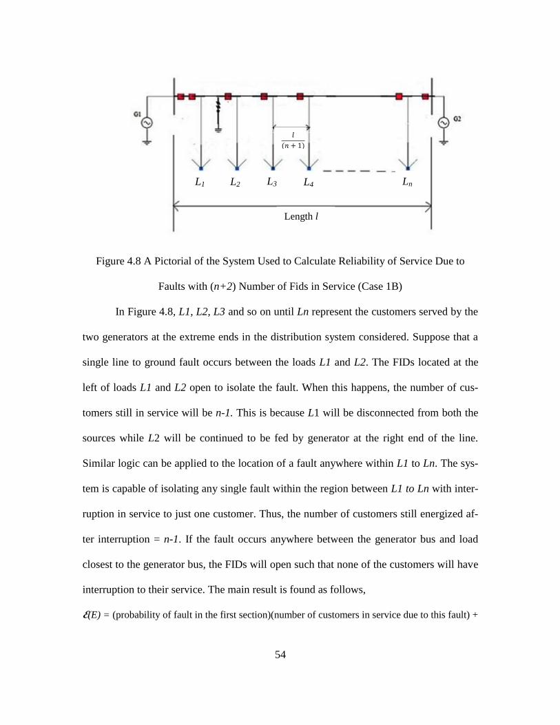
54
Figure 4.8 A Pictorial of the System Used to Calculate Reliability of Service Due to
Faults with (n+2) Number of Fids in Service (Case 1B)
In Figure 4.8, L1, L2, L3 and so on until Ln represent the customers served by the
two generators at the extreme ends in the distribution system considered. Suppose that a
single line to ground fault occurs between the loads L1 and L2. The FIDs located at the
left of loads L1 and L2 open to isolate the fault. When this happens, the number of cus-
tomers still in service will be n-1. This is because L1 will be disconnected from both the
sources while L2 will be continued to be fed by generator at the right end of the line.
Similar logic can be applied to the location of a fault anywhere within L1 to Ln. The sys-
tem is capable of isolating any single fault within the region between L1 to Ln with inter-
ruption in service to just one customer. Thus, the number of customers still energized af-
ter interruption = n-1. If the fault occurs anywhere between the generator bus and load
closest to the generator bus, the FIDs will open such that none of the customers will have
interruption to their service. The main result is found as follows,
E(E) = (probability of fault in the first section)(number of customers in service due to this fault) +
Length l
L1 L2 L3 L4 Ln
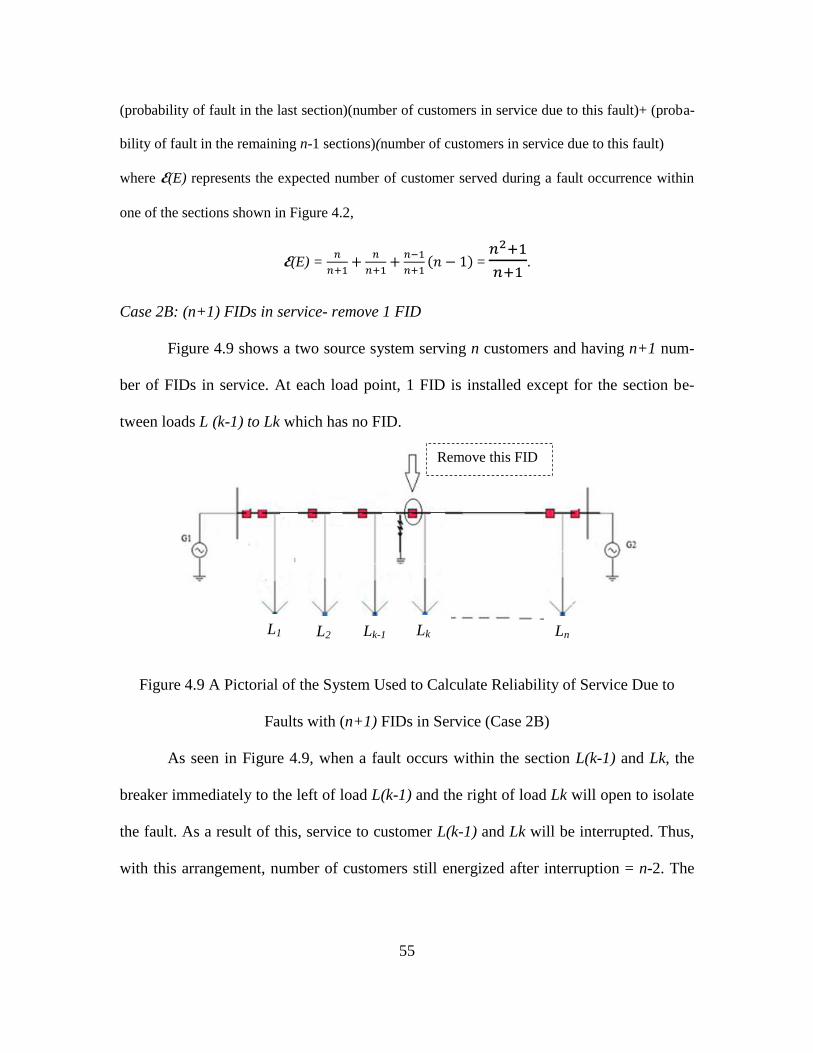
55
(probability of fault in the last section)(number of customers in service due to this fault)+ (proba-
bility of fault in the remaining n-1 sections)(number of customers in service due to this fault)
where E(E) represents the expected number of customer served during a fault occurrence within
one of the sections shown in Figure 4.2,
E(E) =
=
.
Case 2B: (n+1) FIDs in service- remove 1 FID
Figure 4.9 shows a two source system serving n customers and having n+1 num-
ber of FIDs in service. At each load point, 1 FID is installed except for the section be-
tween loads L (k-1) to Lk which has no FID.
Figure 4.9 A Pictorial of the System Used to Calculate Reliability of Service Due to
Faults with (n+1) FIDs in Service (Case 2B)
As seen in Figure 4.9, when a fault occurs within the section L(k-1) and Lk, the
breaker immediately to the left of load L(k-1) and the right of load Lk will open to isolate
the fault. As a result of this, service to customer L(k-1) and Lk will be interrupted. Thus,
with this arrangement, number of customers still energized after interruption = n-2. The
Remove this FID
L1 Lk Ln L2 Lk-1
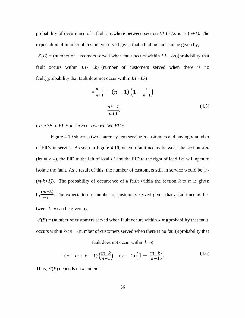
56
probability of occurrence of a fault anywhere between section L1 to Ln is 1/ (n+1). The
expectation of number of customers served given that a fault occurs can be given by,
E (E) = (number of customers served when fault occurs within L1 - Ln)(probability that
fault occurs within L1- Lk)+(number of customers served when there is no
fault)(probability that fault does not occur within L1 - Lk)
=
=
.
(4.5)
Case 3B: n FIDs in service- remove two FIDs
Figure 4.10 shows a two source system serving n customers and having n number
of FIDs in service. As seen in Figure 4.10, when a fault occurs between the section k-m
(let m > k), the FID to the left of load Lk and the FID to the right of load Lm will open to
isolate the fault. As a result of this, the number of customers still in service would be (n-
(m-k+1)). The probability of occurrence of a fault within the section k to m is given
by
. The expectation of number of customers served given that a fault occurs be-
tween k-m can be given by,
E (E) = (number of customers served when fault occurs within k-m)(probability that fault
occurs within k-m) + (number of customers served when there is no fault)(probability that
fault does not occur within k-m)
=
(4.6)
Thus, E (E) depends on k and m.
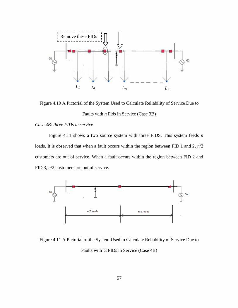
57
Figure 4.10 A Pictorial of the System Used to Calculate Reliability of Service Due to
Faults with n Fids in Service (Case 3B)
Case 4B: three FIDs in service
Figure 4.11 shows a two source system with three FIDS. This system feeds n
loads. It is observed that when a fault occurs within the region between FID 1 and 2, n/2
customers are out of service. When a fault occurs within the region between FID 2 and
FID 3, n/2 customers are out of service.
Figure 4.11 A Pictorial of the System Used to Calculate Reliability of Service Due to
Faults with 3 FIDs in Service (Case 4B)
L1 Lk Lm Ln
Remove these FIDs
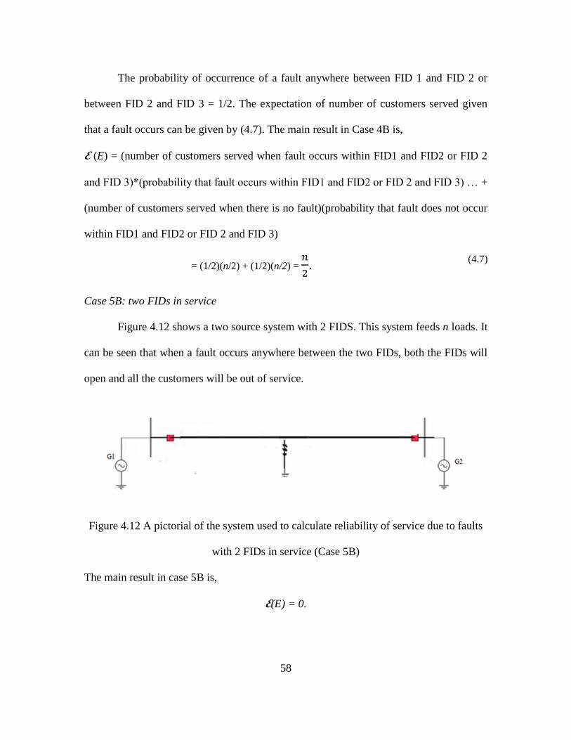
58
The probability of occurrence of a fault anywhere between FID 1 and FID 2 or
between FID 2 and FID 3 = 1/2. The expectation of number of customers served given
that a fault occurs can be given by (4.7). The main result in Case 4B is,
E (E) = (number of customers served when fault occurs within FID1 and FID2 or FID 2
and FID 3)*(probability that fault occurs within FID1 and FID2 or FID 2 and FID 3) … +
(number of customers served when there is no fault)(probability that fault does not occur
within FID1 and FID2 or FID 2 and FID 3)
= (1/2)(n/2) + (1/2)(n/2) =
.
(4.7)
Case 5B: two FIDs in service
Figure 4.12 shows a two source system with 2 FIDS. This system feeds n loads. It
can be seen that when a fault occurs anywhere between the two FIDs, both the FIDs will
open and all the customers will be out of service.
Figure 4.12 A pictorial of the system used to calculate reliability of service due to faults
with 2 FIDs in service (Case 5B)
The main result in case 5B is,
E(E) = 0.
59
4.6 A Closed Form Expression for E(E) for Configuration B
Figure 4.13 can be approximated by a third degree polynomial such that E(E) =
aV3+bV
2+cV+d where V represents the number of FIDs in service. The values of results
obtained in Section 4.5 can be substituted for n = 20 customers. The calculation of value
of the parameters a,b,c and d are explained in Appendix D.
E(E) = 0.0279V3-1.2214V
2+15.4694V-26.226.
The rms error in the approximation can be calculated by,
The value of the rms error for Configuration B is calculated in Appendix D and is
given by (0.5501).
4.7 Summary of Results for Configuration B
Figure 4.13 is a graph of expectation of number of customers served versus num-
ber of FIDs in service. This graph combines the results obtained in cases 1B to 5B as cal-
culated in section 4.5. For the graph, number of customers to be served is taken as n = 20.
Thus, there will be (20) +2 = 22 FIDs in the system. For the intermediate values not cal-
culated in Section 4.5, approximate results are predicted to lie within the extremes calcu-
lated.
4.8 Results for Configuration A and Configuration B
The results for all the test cases considered for both the Configurations A and B
are summarized in Table 4.3.
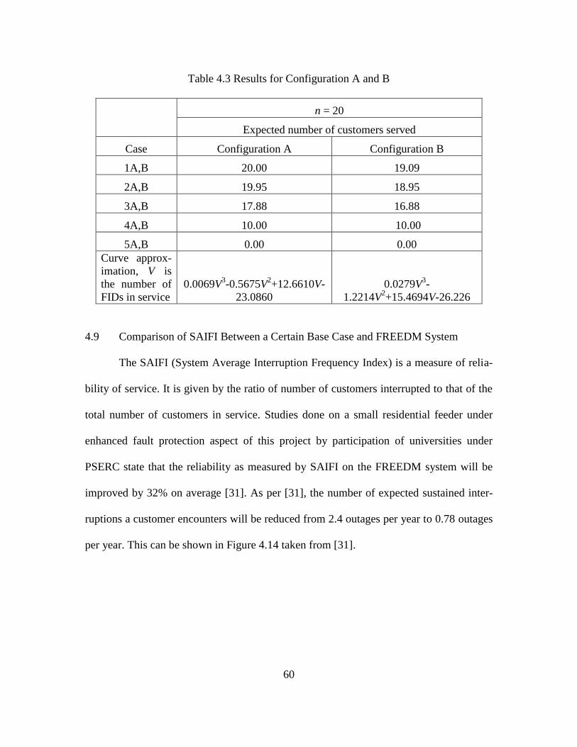
60
Table 4.3 Results for Configuration A and B
n = 20
Expected number of customers served
Case Configuration A Configuration B
1A,B 20.00 19.09
2A,B 19.95 18.95
3A,B 17.88 16.88
4A,B 10.00 10.00
5A,B 0.00 0.00
Curve approx-
imation, V is
the number of
FIDs in service
0.0069V3-0.5675V
2+12.6610V-
23.0860
0.0279V3-
1.2214V2+15.4694V-26.226
4.9 Comparison of SAIFI Between a Certain Base Case and FREEDM System
The SAIFI (System Average Interruption Frequency Index) is a measure of relia-
bility of service. It is given by the ratio of number of customers interrupted to that of the
total number of customers in service. Studies done on a small residential feeder under
enhanced fault protection aspect of this project by participation of universities under
PSERC state that the reliability as measured by SAIFI on the FREEDM system will be
improved by 32% on average [31]. As per [31], the number of expected sustained inter-
ruptions a customer encounters will be reduced from 2.4 outages per year to 0.78 outages
per year. This can be shown in Figure 4.14 taken from [31].
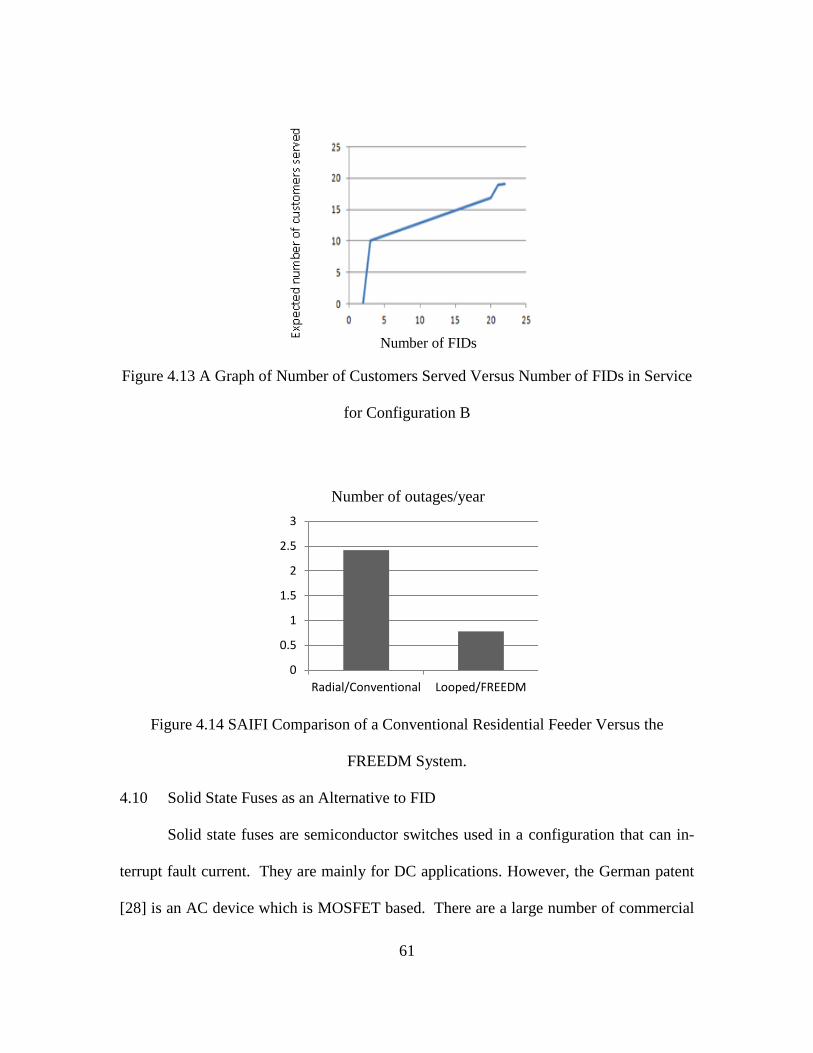
61
Figure 4.13 A Graph of Number of Customers Served Versus Number of FIDs in Service
for Configuration B
Figure 4.14 SAIFI Comparison of a Conventional Residential Feeder Versus the
FREEDM System.
4.10 Solid State Fuses as an Alternative to FID
Solid state fuses are semiconductor switches used in a configuration that can in-
terrupt fault current. They are mainly for DC applications. However, the German patent
[28] is an AC device which is MOSFET based. There are a large number of commercial
0
0.5
1
1.5
2
2.5
3
Radial/Conventional Looped/FREEDM
Number of outages/year
Number of FIDs

62
applications of solid state fuses commercialized by Cooper Bussmann industries. In sin-
gle units, these fuses are available to 7500 A, 1250 V [29]. The use of solid state fuses in
industrial applications remains uncertain. The interrupt speeds are very fast and adhere to
IEC 60269 standards [32]. The costs of such fuses are very much lower than their FID
counterparts.
As specified in Section 1.7, FIDs interrupt fault currents within a few 100 micro-
seconds as compared to about 12 milliseconds for even the fastest operating conventional
circuit breaker. However, C57.1200 [33] states that a fault of 0.25 second has to be ac-
commodated, and NEMA ST20-1992 [30] states that a fault of 2 seconds needs to be ac-
commodated. In C57.1259 [33], it implies 100 ms is a guideline for fuse interruption
which is approximately 6 cycles of operation. This helps in stating that the extreme high
speed protection of FIDs is not quite required and hence a compromise can be made on
reliability by using solid state fuses. The lower level of performance of solid state fuses
could be a real alternative.

63
CHAPTER 5 CALCULATION AND DISCUSSION OF PAYBACK PERIODS
5.1 Introduction
In this chapter an effort is made to quantify the benefits of the FREEDM system
such as enhanced reliability of service to customers, reduction in active power losses in
the feeder as compared to a case with magnetic transformers of the same rating, reduction
in cost due to elimination of capacitor banks as well as reduction in cost due to use of re-
newables. The major investment involved in the FREEDM system comes from the SSTs
and FIDs. As mentioned in Section 3.9, cost of an SST after technology matures can be
estimated to be around 67$/ kVA. The FID cost can range between 12000$-24000$ for
installment in the FREEDM system shown in Figure 3.1 [20]. Estimated cost for a single
15 kV prototype is roughly 50,000$ [37]. The cost of a single FID used for calculation of
payback period for the system shown in Figure 3.1 is taken to be 5000$ assuming reduc-
tion in cost by a factor of 10 when a large scale bulk order is placed for massive commer-
cialization of the FREEDM system as well as after technology matures. A range of cost
of FIDs can also be studied for payback period using the same procedure mentioned in
this chapter. Evaluating the value of providing enhanced reliability of service to custom-
ers in case of the FREEDM system is a difficult process. It is mostly psychological in the
sense that it depends on how much of a disruption in service can be tolerated and also on
how much is the cost of every outage per customer. Research done by the team at North
Carolina State University has calculated the value of outage cost per customer by taking
into consideration the reduction in SAIFI and SAIDI in case of the FREEDM system
when compared to the conventional system [37]. Two values of benefit due to reliability

64
per year per customer are considered to span a range: 40$ and 80$. For the Configura-
tions A and B specified in Chapter 4, two cases are studied:
Case X: No subsidy.
Case Y: Subsidy of 10 % of the customer's annual bill to encourage utilization of
the FREEDM system.
For each of the above cases, the value of benefit due to reliability is varied as
40$/customer/year and 80$/customer/year. The savings due to use of renewables in cost
per year for all the customers is estimated to be around 10 % of the total annual bill of all
the customers. The calculation of payback period is done for the following category of
assumptions:
Cost of a single FID for the system shown in Figure 3.1 is 5000$ [20]. This value
is taking after considering that technology matures as well as reduction in cost
when a mass scale bulk order is placed after going for commercialization of the
FREEDM system.
SST incurs 1 % active power losses at 75 % of loading.
A single 36 kVA magnetic transformer is assumed to operate at 85 % power fac-
tor.
Capacitors used in the system consisting of magnetic transformers shown in Fig-
ure 3.1 improve power factor to unity and cost 35.4$/ kVAr as described in Sec-
tion 3.8.
Value of $ does not change over the course of the payback period.
1% and 2% rates of interest are also taken into consideration while calculating
payback period.
65
5.2 Calculation of Payback Period without Considering Rate of Interest
Consider:
F =
S =
RB = reliability benefit in $ per customer per year number of customers
L = annual reduction in cost of active power losses when compared to system hav
ing conventional transformers
CP = annual reduction in cost due to elimination of installing capacitor banks
H = annual savings in total electricity bill for all customers due to use of renewa-
bles
G = subsidy of 10 % of the total customer's annual bill to encourage utilization of
the FREEDM system
The payback period is calculated by the following formula which is applicable to
both the configurations.
n', Payback period (years) =
(5.1) )
For the case X, the value of G = 0. From the ERCOT loading data, the value of
energy consumed per year per 36 kVA transformer as per APPENDIX A comes out to be
around 177.24 MWh/year. The average value of cost of energy taken to be approximately
10 cents/kWh as mentioned in Chapter 3 gives the annual cost of energy per transformer
to be around 17,700$/year. The FREEDM system assumed in Figure 3.1 has 20 custom-
ers with each transformer serving 3 residences. Thus, total cost of energy per year for all
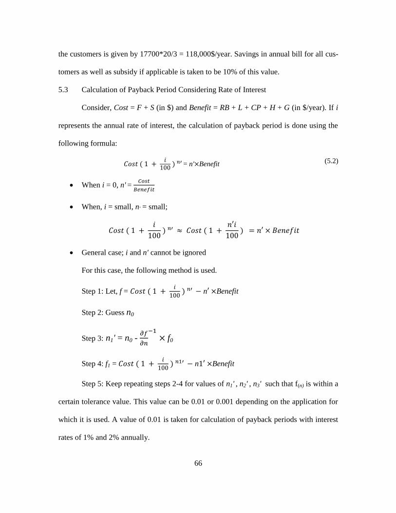
66
the customers is given by 17700*20/3 = 118,000$/year. Savings in annual bill for all cus-
tomers as well as subsidy if applicable is taken to be 10% of this value.
5.3 Calculation of Payback Period Considering Rate of Interest
Consider, Cost = F + S (in $) and Benefit = RB + L + CP + H + G (in $/year). If i
represents the annual rate of interest, the calculation of payback period is done using the
following formula:
= n' Benefit (5.2)
When i = 0, n' =
When, i = small, n' = small;
General case; i and n' cannot be ignored
For this case, the following method is used.
Step 1: Let, f =
n Benefit
Step 2: Guess n0
Step 3: n1' = n0 -
f0
Step 4: f1 =
n Benefit
Step 5: Keep repeating steps 2-4 for values of n1' , n2' , n3' such that f(n) is within a
certain tolerance value. This value can be 0.01 or 0.001 depending on the application for
which it is used. A value of 0.01 is taken for calculation of payback periods with interest
rates of 1% and 2% annually.

67
5.4 Results
The calculations for both cases X and Y for Configurations A and B are illustrated
in Appendix E. These calculations are done for the following rates of interest: i = 0%, i =
1% and i = 2%. The results are tabulated in Table 5.1.
5.5 Summary and Conclusions
It is observed from the results tabulated in Table 5.1 that the fastest payback peri-
od of 5.82 years is expected for the enhanced reliability case for Configuration B without
taking the rate of interest into consideration. The longest payback period of 36.45 years is
observed for Configuration A with an annual rate of interest of 2% and for the lower
range of reliability case. These results make sense as Configuration B has almost half the
number of FIDs as Configuration A and hence the cost of the system in Configuration B
is a lot less than that of Configuration A. Also, as the rate of interest gets introduced in
the calculations, the payback period will increase. A payback period of 5 - 10 years for
the FREEDM system is justified. According to that philosophy, adopting the FREEDM
system thus would be viable.
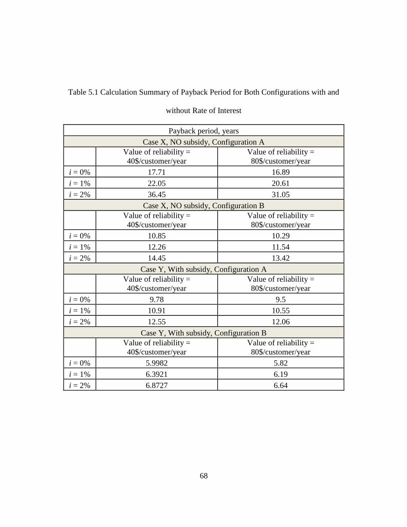
68
Table 5.1 Calculation Summary of Payback Period for Both Configurations with and
without Rate of Interest
Payback period, years
Case X, NO subsidy, Configuration A
Value of reliability =
40$/customer/year
Value of reliability =
80$/customer/year
i = 0% 17.71 16.89
i = 1% 22.05 20.61
i = 2% 36.45 31.05
Case X, NO subsidy, Configuration B
Value of reliability =
40$/customer/year
Value of reliability =
80$/customer/year
i = 0% 10.85 10.29
i = 1% 12.26 11.54
i = 2% 14.45 13.42
Case Y, With subsidy, Configuration A
Value of reliability =
40$/customer/year
Value of reliability =
80$/customer/year
i = 0% 9.78 9.5
i = 1% 10.91 10.55
i = 2% 12.55 12.06
Case Y, With subsidy, Configuration B
Value of reliability =
40$/customer/year
Value of reliability =
80$/customer/year
i = 0% 5.9982 5.82
i = 1% 6.3921 6.19
i = 2% 6.8727 6.64

69
CHAPTER 6 CONCLUSIONS AND RECOMMENDATIONS
6.1 Conclusions
This thesis focuses on a future power distribution system, the FREEDM system.
Electronic controls are used in the FREEDM system. Active power losses for a distribu-
tion feeder are calculated for both the FREEDM and conventional systems. The conven-
tional system uses magnetic transformers; the FREEDM system uses SSTs. A reduction
in the active power losses in the feeder of about a maximum of 18.76% is observed in
case of the FREEDM system. A savings of about a maximum of 47.6 % in the cost of
FIDs can be obtained by changing the configuration from A to B, by serving one load
point less which typically consists of 3-4 residences. A further study regarding the effect
of storage devices in coping with this contingency of loss of one load point as well as the
duration for which the service is out needs to be quantitatively conducted. In [31], the
reliability of a conventional system is compared with that of the proposed FREEDM sys-
tem. The main observation relating to reliability is an improvement of 32% for the
FREEDM system in terms of SAIFI.
A second area of comparison for the FREEDM system relates to cost/benefit,
namely the payback period. For the FREEDM system, an optimistic value of payback
period is 5.82 years. For a less optimistic scenario, the FREEDM system payback period
is longer. The longest value of payback period for a scenario with reduced value of relia-
bility is 36.45 years. A maximum of 10 years for payback period may be acceptable for
the commercialization of the FREEDM system. The study in this thesis includes alterna-
tives relating to
Subsidy

70
Rate of interest
Configuration/design
The different values of payback periods are listed in Table 5.1. Configuration B is
an alternative with approximately one-half the number of FIDs of that in Configuration
A, and Configuration B has a lower value of payback period due to reduced number of
FIDs by about 5.89 years. This reduction in payback period could be an alternative to
Configuration A. Introducing the rate of interest increases the time required for payback
typically by about three years. The payback period calculated without considering subsi-
dy given by the state can increase by a maximum of 15 years when compared with that
calculated with subsidy.
6.2 Recommendations and Future Work
The value of the dollar can be taken into account while evaluating the payback
periods. The FIDs are cost intensive and technology needs to develop cheaper solutions
that can introduce functionalities similar to that of the piezoelectric FIDs considered for
the FREEDM system. A strong contender for FIDs could be solid state fuses.
The main recommendations for future work relating to the cost/benefit analysis of
the FREEDM system are:
Put the cost/benefit analysis into a real neighborhood setting, calculating the bene-
fits and costs to the distribution supplier and home owner.
Resolve the question of whether less expensive FID components are suitable for
this application.
Expand the sensitivity studies shown in this thesis by adding to the scenarios stud-
ied.

71
Resolve any differences between cost/benefit analysis shown here and those con-
ducted elsewhere.
Add the benefit of DESD as well as real time load monitoring and management
to this study.
A study of the benefits if solar or wind is added needs to be conducted.
A "cost" of SST failure versus a conventional transformer should be included.
Identify what possible configurations can be used apart from the configurations A
and B mentioned in this study.
Include the costs of relay circuits used to trip the FID.
What was studied is a single phase
equivalent, a study needs to be done to
observe what happens in a real three phase 15 kV case.
Include the study of re-closers and fuses in both the configurations.
72
REFERENCES
[1] Next Generation Power Distribution System Architecture, “The Future Renewable
Electric Energy Delivery and Management (FREEDM) System”. [Online], available:
http://www.thinkmind.org/index.php?view=article&articleid=energy_2013_2_40_40
134
[2] FREEDM systems center, “About: FREEDM Systems”. [Online], available:
http://www.freedm.ncsu.edu/index.php?s=1&p=6
[3] H. P. Barringer, P. E. Barringer & Associates, Inc. “A Life Cycle Cost Summary,”
Humble, Texas.
[4] R. Reis, “Pros and Cons of Performing a Cost-Benefit Analysis,” [Online], available:
http://www.docstoc.com/article/98795770/Pros-and-Cons-of-Performing-a-Cost
Benefit- Analysis
[5] J. E. Huber, J. W. Kolar, “Volume/Weight/Cost Comparison of a 1 MVA 10kV/400
V Solid-State against a Conventional Low-Frequency Distribution Transformer,”
IEEE Energy Conversion Congress and Exposition, 2014, pp. 4545 – 4552.
[6] G. G. Karady, A. Q. Huang, M. Baran, “FREEDM System: An Electronic Smart
Distribution Grid For The Future,” IEEE Transmission and Distribution Conference
and Exposition 2012, pp. 1 – 6.
[7] X. She, R. Burgos, G.Wang, F.Wang, A. Q.Huang, “Review of Solid State Trans-
former in the Distribution System: From Components to Field Application,”
IEEE Energy Conversion Congress and Exposition (ECCE), 2012, pp. 4077-4084.
[8] X. She, A. Q. Huang, S. Bhattacharya, M. Baran, “Performance Evaluation of Solid
State Transformer based Micro Grid in FREEDM Systems,” IEEE Applied Power
Electronics Conference and Exposition (APEC), 2011, pp. 182-188.
[9] S. B. Y. Du, G. Wang, S. Bhattacharya, “Design Considerations of High Voltage and
High Frequency Transformer for Solid State Transformer Application,” IECON
36th Annual Conference on IEEE Industrial Electronics Society, 2010, pp. 421-426.
[10] FREEDM systems center, “News and Events: Solid-State Transformers Ready to
Enable the Smart Grid?”. [Online], available:
http://www.freedm.ncsu.edu/index.php?s=2&t=news&p=121
[11] A. Q. Huang, “Wide Bandgap Power Semiconductor Devices and Future Electric
Power Delivery System”. [Online], available:
http://nanohub.org/resources/21309/watch?resid=21310
73
[12] U.S. Department of Energy. “Smart Grid / Department of Energy,” [Online], availa-
ble:
http://energy.gov/sites/prod/files/oeprod/DocumentsandMedia/DOE_SG_Book_Sing
le_Pages%281%29.pdf
[13] ERCOT, “Hourly Load Data Archives,” [Online], available:
http://www.ercot.com/gridinfo/load/load_hist/
[14] U.S. Energy Information Administration, “Annual Energy Outlook 2012”, [Online],
available: http://www.eia.gov/forecasts/aeo/pdf/0383 (2012).pdf
[15] U.S. Department of Energy, “Supplement to the “Determination Analysis” (ORNL-
6847) and Analysis of the NEMA Efficiency Standard for Distribution Transform-
ers”, [Online], available: http://www.eia.gov/forecasts/aeo/pdf/0383(2012).pdf
[16] Westinghouse Electric Co., “Electrical Transmission and Distribution Reference
Book,” Westinghouse, Pittsburgh, PA, 1965.
[17] M. Kempkes, I. Roth, M. Gaudreau, “Solid-State Circuit Breakers For Medium
Voltage DC Power,” IEEE Electric Ship Technologies Symposium (ESTS), 2011,
pp. 254-257.
[18] M. K. Madan and B. H. Chowdhury, “Study of Solid State Fault Interruption Device
for Medium Voltage Distribution Systems with Distributed Generators,” IEEE
Power and Energy Society General Meeting, 2010, pp. 1-7.
[19] O. Vodyakho, M. Steurer, C. Edrington, G. Karady, B. Chowdhury and S.
Bhattacharya, “Design of a Solid State Fault Isolation Device for Implementation in
Power Electronics based Distribution Systems,” North American Power Symposium,
2009, pp. 1-6.
[20] FREEDM conference call, “Cost/Benefit Project-ItemizedParts_updatedJan20.xls,”
02/27/2015.
[21] G. Strbac, N. Jenkins, “Calculation of Cost and Benefits to the Distribution Network
of Embedded Generation,” IEE Colloquium on Economics of Embedded Genera-
tion, 1998, pp. 6/1 – 6/13.
[22] Y. Yang, N. Yang, H. Li, “Cost-benefit Study of Dispersed Battery Storage to In-
crease Penetration of Photovoltaic Systems on Distribution Feeders,” IEEE PES
General Meeting, 2014, pp. 1 – 5.
[23] C. Yang, P. Hu, Y. He, “Research on Cost-Benefit Analysis and Evaluation of Re-
gional Distribution Network Planning,” China International Conference on Elec-
tricity Distribution, 2010, pp. 1 – 6.

74
[24] S. Umans, W. Fitzgerald, G. Kingsley, “Electric Machinery,” The McGraw Hill
Companies, Delhi, India, 2013.
[25] D. P. Kothari, I. J. Nagrath, “Electrical Machines,” The McGraw Hill Companies,
Delhi, India, 2008.
[26] S. Chapman, “Electric Machinery Fundamentals,” BAE Systems Australia.
[27] F. Ioan, R. Nicolae, H. Viorel, “Experimental Correction of Transformer Losses
which Operates in Harmonic Regime,” IET Conference Publications, 20th In-
ternational Conference and Exhibition on Electricity Distribution - Part 1, 2009, pp.
1-4.
[28] M. Feldtkeller, “Electronic Fuse (protection device) DE 3705177 A1,” Siemens Ag,
Application no. DE19873705177, Germany, 1987.
[29] “High Speed Fuses,” Cooper Bussmann Industries, [Online], available:
http://www.cooperindustries.com/content/dam/public/bussmann/Electrical/Resourc
es/solution-center/technical_library/BUS_Ele_Tech_Lib_High_Speed_Fuses.pdf
[30] National Electrical Manufacturers Association, 2007, [Online], available:
http://infostore.saiglobal.com/store/Details.aspx?productID=1748487
[31] M. Baran, L. White, G. Heydt, M. Crow, S. Bhattacharya, M. Steurer, “Volume II-
Core Project Summary,” Cost-Benefit project, FREEDM, 2015.
[32] International Electrotechnical Commission, “International IEC Standard 60269-1,”
Reference Number IEC 60269-1:2006(E), Geneva, 2006.
[33] Waukesha Electric Systems, “New Diagnostic Concepts for Better Asset Manage-
ment,” Weidmann-ACTI Inc. Technical Conference, 2005, [Online], available:
http://www.weidmannsolutions.cn/huiyi/Seminar%202005%20San%20Antonio/200
5simpresentation.pdf
[34] A. Kusko, M. Thompson, “Power Quality in Electrical Systems,” McGraw-Hill,
New York, 2007.
[35] J. Kyei, “Analysis and Design of Power Acceptability Curves for Industrial Loads,”
Power Systems Engineering Research Center, New York, 2001.
[36] G. T. Heydt, “Electric Power Quality,” Stars in a Circle, West Lafayette, Indiana,
1991.

75
[37] M. Baran, L. White, G. Heydt, M. Crow, S. Bhattacharya, M. Steurer, “FREEDM
System Cost-Benefit Analysis,” Site Visit Presentation, Year 07, Cost-Benefit pro-
ject, FREEDM, 2015.

76
APPENDIX A
LOSS CALCULATION FOR A 36 KVA MAGNETIC TRANSFORMER

77
clc;
clear all;
close all;
cost=10.27 % cents/kwh as per data for the year 2012
% Also considering a 36 KVA distribution transformer in service.
rating=36000; % base rating of the distribution transformer
r1=0.0178; % per unit resistance
sum=0;
load = importfile4('2013_ERCOT_Hourly_Load_Data.xls','2013',2,8761);
for i=1:8760
load(i)=load(i)*10^6;
sum=sum+load(i);
end
pmax=max(load)
load_factor=sum/(pmax*8760)
%Actual Load on the transformer is denoted by load1
%Calculate the load on the transformer for all the 8760 hours
% of the year and store it in the matrix load1
for i=1:8760
load_size_kw(i)= load(i)*rating/pmax;
end
a=max(load_size_kw)
b=min(load_size_kw)
% Calculate the value of per unit current flowing through the
% transformer for every hour as well as the losses per hour in per unit
% as per loading on the transformer calculated above.
c1=0;c2=0;c3=0;
for i=1:8760
current_pu_1(i)= load_size_kw(i)/(rating*1);
current_pu_2(i)= load_size_kw(i)/(rating*0.85);
current_pu_3(i)= load_size_kw(i)/(rating*0.6);
loss_pu1(i)=current_pu_1(i)*current_pu_1(i)*r1;
loss1(i)=loss_pu1(i)*rating;
c1=c1+loss1(i);
loss_pu2(i)=current_pu_2(i)*current_pu_2(i)*r1;
loss2(i)=loss_pu2(i)*rating;
c2=c2+loss2(i);
loss_pu3(i)=current_pu_3(i)*current_pu_3(i)*r1;
loss3(i)=loss_pu3(i)*rating;
c3=c3+loss3(i);

78
end
display('Energy lost per year for the 36 KVA transformer operating at unity power factor
is as follows');
c1
display('Cost of Energy lost per year for the 36 KVA transformer operating at unity pow-
er factor in$/year is as follows')
cost*c1*10^-5
display('Energy lost per year for the 36 KVA transformer operating at 85 % factor is as
follows');
c2
display('Cost of Energy lost per year for the 36 KVA transformer operating at 85 % pow-
er factor in$/year is as follows')
cost*c2*10^-5
display('Energy lost per year for the 36 KVA transformer operating at 60 % power factor
is as follows');
c3
display('Cost of Energy lost per year for the 36 KVA transformer operating at 60 % pow-
er factor in$/year is as follows')
cost*c3*10^-5
OUTPUT
cost = 10.2700
pmax = 6.7596e+10
load_factor = 0.5620
a = 36000
b = 1.2484e+04
Energy lost per year for the 36 KVA transformer operating at unity power factor is as fol-
lows
c1 = 1.8723e+06
Cost of Energy lost per year for the 36 KVA transformer operating at unity power factor
in$/year is as follows
ans = 192.2815
Energy lost per year for the 36 KVA transformer operating at 85 % factor is as follows
c2 = 2.5914e+06

79
Cost of Energy lost per year for the 36 KVA transformer operating at 85 % power factor
in$/year is as follows
ans = 266.1336
Energy lost per year for the 36 KVA transformer operating at 60 % power factor is as fol-
lows
c3 = 5.2007e+06
Cost of Energy lost per year for the 36 KVA transformer operating at 60 % power factor
in$/year is as follows
ans = 534.1153

80
APPENDIX B
LOSS CALCULATION FOR A 36 KVA SST

81
clc;
clear all;
close all;
cost=10.27 % cents/kwh as per data for the year 2012
% Also considering a 36 KVA distribution transformer in service.
rating=36000; % rating of the distribution transformer
r=0.0178; % per unit resistance
% Considering 5 % loss at 75 % Load
a1=0.0556;
b1=0.0148148;
% Considering 1 % loss at 75 % Load
a2=0.01111;
b2=2.96296*10^-3;
load = importfile4('2013_ERCOT_Hourly_Load_Data.xls','2013',2,8761);
for i=1:8760
load(i)=load(i)*10^6;
end
pmax=max(load)
% Load on the transformer is denoted by load1
% Calculate the load on the transformer for all the 8760 hours
% of the year and store it in the matrix load1
for i=1:8760
load1(i)= load(i)*rating/pmax;
end
a=max(load1)
b=min(load1)
% Calculate the value of per unit current flowing through the
% transformer for every hour as well as the losses per hour in per unit
% as per loading on the transformer calculated above.
c=0;d=0;
for i=1:8760
current_pu(i)=load1(i)/rating;
loss_pu(i)=a1*current_pu(i)+(b1*current_pu(i)*current_pu(i));
loss(i)=loss_pu(i)*rating;
c=c+loss(i);

82
loss_pu_1(i)=a2*current_pu(i)+(b2*current_pu(i)*current_pu(i));
loss_1(i)=loss_pu_1(i)*rating;
d=d+loss_1(i);
end
display('Energy lost per year for the 36 KVA SST transformer for 5 % losses at 75 %
load is as follows');
c
display('Cost of Energy lost per year for the 36 KVA transformer in$/year is as follows')
cost*c*10^-5
display('Energy lost per year for the 36 KVA SST transformer for 1 % losses at 75 %
load is as follows');
d
display('Cost of Energy lost per year for the 36 KVA transformer in$/year is as follows')
cost*d*10^-5
OUTPUT
cost = 10.2700
pmax = 6.7596e+10
a = 36000
b = 1.2484e+04
Energy lost per year for the 36 KVA SST transformer for 5 % losses at 75 % load is as
follows
c = 1.1413e+07
Cost of Energy lost per year for the 36 KVA transformer in$/year is as follows
ans = 1.1721e+03
Energy lost per year for the 36 KVA SST transformer for 1 % losses at 75 % load is as
follows
d = 2.2808e+06
Cost of Energy lost per year for the 36 KVA transformer in $/year is as follows
ans = 234.2413

83
APPENDIX C
ANNUAL ENERGY LOST IN FEEDER USING DISTRIBUTION LEVEL MAGNET-
IC TRANSFORMERS AND SSTS

84
clc;
clear all;
close all;
rating=36000; % rating of the distribution transformer
cost=10.27; % cents/kwh as per data for the year 2012
load = importfile4('2013_ERCOT_Hourly_Load_Data.xls','2013',2,8761);
for i=1:8760
load(i)=load(i)*10^6;
end
pmax=max(load);
%Actual Load on the transformer is denoted by load1
% Calculate the load on the transformer for all the 8760 hours
% of the year and store it in the matrix load1
for i=1:8760
load1(i)= load(i)*rating/pmax;
current_sst(i)= load1(i)*sqrt(3)/(15000);
current_magnetic(i)= load1(i)*sqrt(3)/(15000*0.85);
end
sum1_mag=0;
sum1_sst=0;
for k=1:8760
sum_mag(k)=0;
sum_sst(k)=0;
r=1.41; % ohms per mile
d=11;
summ_mag=0;
summ_sst=0;
for n=1:11
c=1.41*10/19 ;
ploss_mag(n)=c*d*d*current_magnetic(k)*current_magnetic(k);
ploss_sst(n)=c*d*d*current_sst(k)*current_sst(k);
d=d-1;
summ_mag=summ_mag+ploss_mag(n);
summ_sst=summ_sst+ploss_sst(n);
end
sum_mag(k)=summ_mag;
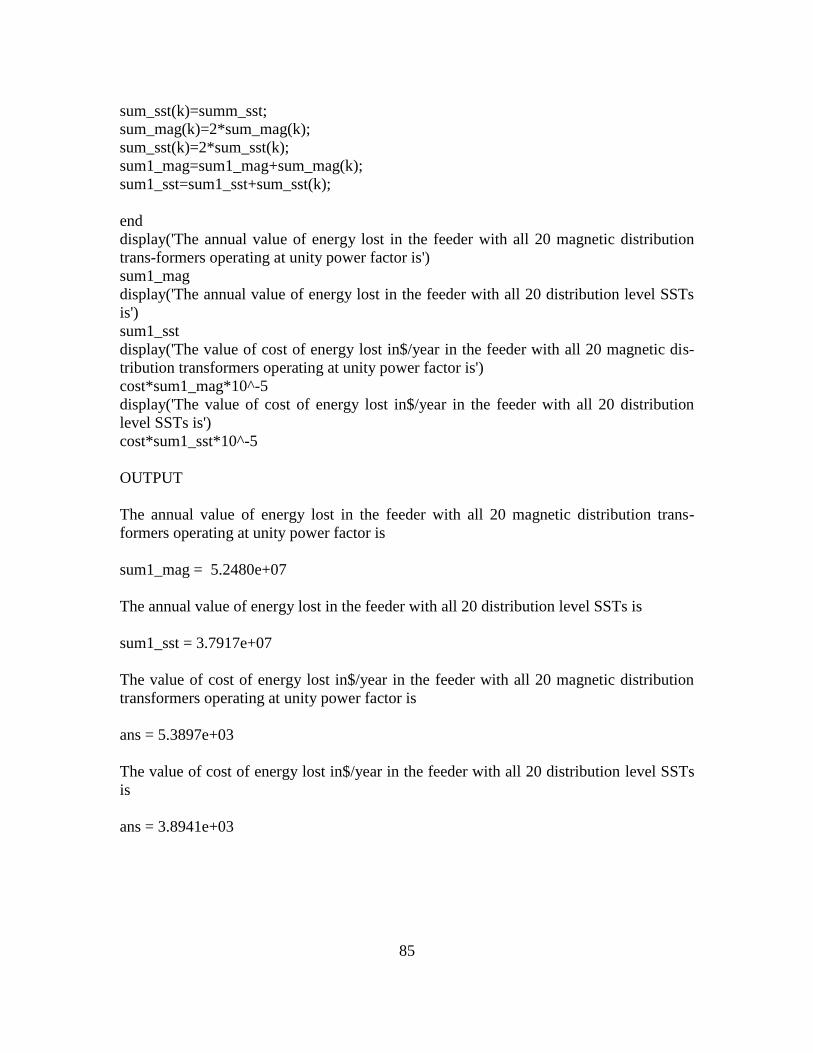
85
sum_sst(k)=summ_sst;
sum_mag(k)=2*sum_mag(k);
sum_sst(k)=2*sum_sst(k);
sum1_mag=sum1_mag+sum_mag(k);
sum1_sst=sum1_sst+sum_sst(k);
end
display('The annual value of energy lost in the feeder with all 20 magnetic distribution
trans-formers operating at unity power factor is')
sum1_mag
display('The annual value of energy lost in the feeder with all 20 distribution level SSTs
is')
sum1_sst
display('The value of cost of energy lost in$/year in the feeder with all 20 magnetic dis-
tribution transformers operating at unity power factor is')
cost*sum1_mag*10^-5
display('The value of cost of energy lost in$/year in the feeder with all 20 distribution
level SSTs is')
cost*sum1_sst*10^-5
OUTPUT
The annual value of energy lost in the feeder with all 20 magnetic distribution trans-
formers operating at unity power factor is
sum1_mag = 5.2480e+07
The annual value of energy lost in the feeder with all 20 distribution level SSTs is
sum1_sst = 3.7917e+07
The value of cost of energy lost in$/year in the feeder with all 20 magnetic distribution
transformers operating at unity power factor is
ans = 5.3897e+03
The value of cost of energy lost in$/year in the feeder with all 20 distribution level SSTs
is
ans = 3.8941e+03

86
APPENDIX D
CURVE APPROXIMATION OF RELIABILITY CALCULATIONS FOR CONFIGU-
RATIONS A AND B

87
clc;
clear all;
close all;
A=[42*42*42 42*42 42 1; 41*41*41 41*41 41 1; 40*40*40 40*40 40 1; 3*3*3 3*3 3 1;
2*2*2 2*2 2 1];
D=[22*22*22 22*22 22 1; 21*21*21 21*21 21 1; 20*20*20 20*20 20 1; 3*3*3 3*3 3 1;
2*2*2 2*2 2 1];
B=[19.09;18.952;16.88;10;0]; % config B
C=[20;19.95;17.8819;10;0]; % config A
E=pinv(A)*C % config A
F=pinv(D)*B % Config B
expected(1)=E(1)*42*42*42+E(2)*42*42+E(3)*42+E(4);
expected(2)=E(1)*41*41*41+E(2)*41*41+E(3)*41+E(4);
expected(3)=E(1)*40*40*40+E(2)*40*40+E(3)*40+E(4);
expected(4)=E(1)*3*3*3+E(2)*3*3+E(3)*3+E(4);
expected(5)=E(1)*2*2*2+E(2)*2*2+E(3)*2+E(4);
expected_b(1)=F(1)*22*22*22+F(2)*22*22+F(3)*22+F(4);
expected_b(2)=F(1)*21*21*21+F(2)*21*21+F(3)*21+F(4);
expected_b(3)=F(1)*20*20*20+F(2)*20*20+F(3)*20+F(4);
expected_b(4)=F(1)*3*3*3+F(2)*3*3+F(3)*3+F(4);
expected_b(5)=F(1)*2*2*2+F(2)*2*2+F(3)*2+F(4);
sum_a=0;
sum_b=0;
for i=1:5
x=(C(i)-expected(i))^2;
sum_a=sum_a+x;
y=(B(i)-expected_b(i))^2;
sum_b=sum_b+y;
end
error_a=sqrt(0.2*(sum_a))
error_b=sqrt(0.2*(sum_b))
OUTPUT
E = 0.0069
-0.5675
12.6610
-23.0860

88
F = 0.0279
-1.2214
15.4694
-26.2260
error_a = 0.4725
error_b = 0.5501

89
APPENDIX E
CALCULATION OF PAYBACK PERIOD WITH INTEREST RATES FOR CONFIG-
URATIONS A AND B

90
clc; clear all; close all; % Assuming configuration A c = 258240; b = 14581.17; i=0.02; n(1) = 5.653009395; f(1)= c*(1.02)^n(1)-b*n(1); i=1; tolerance =1; while (tolerance >= 0.01) df(i)=c*(1.02)^n(i)*log(1.02)-b; n(i+1)=n(i)-((df(i))^-1*f(i)); f(i+1)=c*(1.02)^n(i+1)-b*n(i+1); tolerance = f(i+1) n(i)=n(i+1); f(i)=f(i+1); end n(i)
OUTPUT
tolerance = 3.6045e+04
tolerance = 4.0156e+03
tolerance = 91.6292
tolerance = 0.0531
tolerance = 1.7928e-08
ans = 36.4530
clc; clear all; close all; % Assuming configuration A c = 158240; b = 14581.17; i=0.02; n(1) = 5.653009395; f(1)= c*(1.02)^n(1)-b*n(1);

91
i=1; tolerance =1; while (tolerance >= 0.01) df(i)=c*(1.02)^n(i)*log(1.02)-b; n(i+1)=n(i)-((df(i))^-1*f(i)); f(i+1)=c*(1.02)^n(i+1)-b*n(i+1); tolerance = f(i+1) n(i)=n(i+1); f(i)=f(i+1); end n(i)
OUTPUT
tolerance = 2.6776e+03
tolerance = 2.7124
tolerance = 2.8041e-06
ans = 14.4467

92
APPENDIX F
SUMMARY OF ALL THE TEST CASES USED

93
Case A) Evaluation of losses in a 36 kVA SST: 5% loss at 75% load, Chapter 2
Case B) Evaluation of losses in a 36 kVA SST: 1% loss at 75% load, Chapter 2
Case 1) Improving power factor from 60% to 85% by introducing capacitor banks, Chap-
ter 3
Case 2) Improving power factor from 85% to 100% by introducing capacitor banks,
Chapter 3
Case 3) Improving power factor from 60% to 100% by introducing capacitor banks,
Chapter 3
Case 1A) Reliability of service to customer calculations for (2n + 2) FIDs and Configura-
tion A, Chapter 4
Case 2A) Reliability of service to customer calculations for (2n + 1) FIDs and Configura-
tion A, Chapter 4
Case 3A) Reliability of service to customer calculations for (2n) FIDs and Configuration
A, Chapter 4
Case 4A) Reliability of service to customer calculations for 3 FIDs and Configuration A,
Chapter 4
Case 5A) Reliability of service to customer calculations for 2 FIDs and Configuration A,
Chapter 4
Case 1B) Reliability of service to customer calculations for (2n + 2) FIDs and Configura-
tion B, Chapter 4
Case 2B) Reliability of service to customer calculations for (2n + 1) FIDs and Configura-
tion B, Chapter 4

94
Case 3B) Reliability of service to customer calculations for (2n) FIDs and Configuration
B, Chapter 4
Case 4B) Reliability of service to customer calculations for 3 FIDs and Configuration B,
Chapter 4
Case 5B) Reliability of service to customer calculations for 2 FIDs and Configuration B,
Chapter 4
Case X) Calculation of payback period without any subsidy, Chapter 5
Case Y) Calculation of payback period with 10% subsidy in electricity bill, Chapter 5
Table F.1 shows a summary of all the cases studied in this thesis.
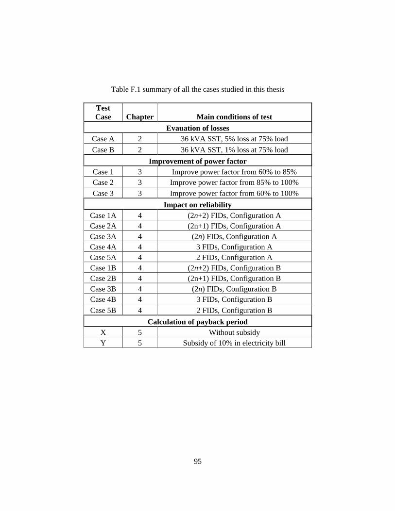
95
Table F.1 summary of all the cases studied in this thesis
Test
Case Chapter Main conditions of test
Evauation of losses
Case A 2 36 kVA SST, 5% loss at 75% load
Case B 2 36 kVA SST, 1% loss at 75% load
Improvement of power factor
Case 1 3 Improve power factor from 60% to 85%
Case 2 3 Improve power factor from 85% to 100%
Case 3 3 Improve power factor from 60% to 100%
Impact on reliability
Case 1A 4 (2n+2) FIDs, Configuration A
Case 2A 4 (2n+1) FIDs, Configuration A
Case 3A 4 (2n) FIDs, Configuration A
Case 4A 4 3 FIDs, Configuration A
Case 5A 4 2 FIDs, Configuration A
Case 1B 4 (2n+2) FIDs, Configuration B
Case 2B 4 (2n+1) FIDs, Configuration B
Case 3B 4 (2n) FIDs, Configuration B
Case 4B 4 3 FIDs, Configuration B
Case 5B 4 2 FIDs, Configuration B
Calculation of payback period
X 5 Without subsidy
Y 5 Subsidy of 10% in electricity bill


![Principles and Standards for Benefit–Cost Analysis] Introduction- Professionalizing Benefit–Cost Analysis](https://img.pdfslide.us/doc/110x75/56d6beb21a28ab30169333bb/principles-and-standards-for-benefitcost-analysis-introduction-professionalizing.jpg)