Embed Size (px)
Citation preview

A Cost Effective Load Balancing Scheme for
Better Resource Utilization in Cloud Computing
K.PushpaLatha Student, M.Phil(Computer Science)
Noorul Islam Centre of Higher Education, Thucklay, India
Dr. R. S. Shaji Professor, Information Technology,
Noorul Islam Centre of Higher Education, Thucklay, India
J. P. Jayan Assistant Professor, Department of Software Engineering
Noorul Islam Centre of Higher Education, Thucklay, India
Abstract—Cloud computing is a new rising paradigm,
consists a pool of virtual resources for cloud users, where
they can access, build and use different operations as per
their need by just agree upon the contract called Service
Level Agreement (SLA) with the cloud provider. Task
Allocation and Storage Distribution are the two discussable
issues while talking about cloud storage (Collection of
VMs).Thus it is very important to the cloud provider for
choosing highly efficient and maximum profitable
scheduling and load leveling strategy to allocate resources to
the various customers for their different operations. In this
article a cost effective load balancing scheme for cloud
computing is proposed that increases the performance of the
resources by decreasing migration time and response time.
The proposed system has a new task scheduling with load
balancing technique (TSLB algorithm) associated with
compression technique to increase resource utilization and
to speed up the process.
IndexTerms—task scheduling, load balancing, cloud
computing,compression.
I. INTRODUCTION
A. Cloud Computing
In the computer world, very latest and commonly
pronounceable term by the many is “Cloud computing”. A
computing system consists of number of interconnected
virtual machines to process different tasks from different
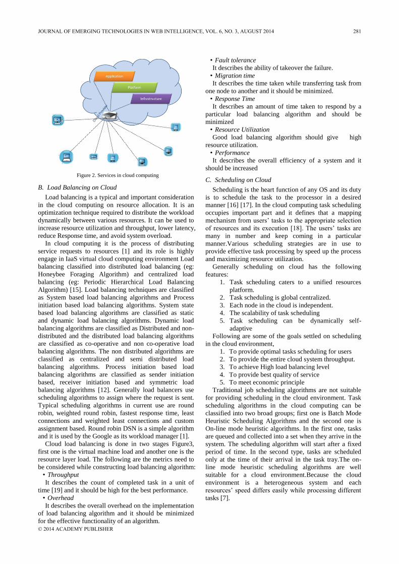
users called cloud. Cloud computing includes three major
components Figure 1 named Datacenters, servers and
virtual machines. A cloud contains multiple of datacenters,
each datacenter contains group of servers and each server
is extended by different number of virtual machines. By
using these components it provided three kinds of services
Figure 2 to its clients. They are, Infrastructure as a Service
(IaaS) for providingvirtualized storage, hardware, servers
and networking componentseg: Amazon Elastic Compute
Cloud, Platform as a Service(PaaS) for application
platforms and databases as a serviceeg: Google
AppEngine and Software as a Service(SaaS) for installing,
running and maintaining software in the cloud eg: Google
AppEngine. These services are facilitates that access
software, applications, and data, build their own software,
application and infrastructure, use the storage and
resources in a very safe and less complexity manner.
Since it is a place of very large, scalable and virtual
resources in the parallel and distributed computing
environment, its clients are allowed to use these resources
for performing their tasks. For using those resources the
clients need to make an agreement with the cloud
provider called SLA. By this agreement the cloud
provider takes some rent from the clients for the
resources used by them. So it is called as a pay-per-use-
on-demand internet system. By the increasing clients with
multiple tasks in the cloud computing it is important to
manage virtual resources in an effective way to avoid
resource wastage and the virtual manager is responsible
for selecting a superlative scheduling with load balancing
plan.
Figure 1. Components in cloud computing
280 JOURNAL OF EMERGING TECHNOLOGIES IN WEB INTELLIGENCE, VOL. 6, NO. 3, AUGUST 2014
© 2014 ACADEMY PUBLISHERdoi:10.4304/jetwi.6.3.280-290
B. Load Balancing on Cloud
Load balancing is a typical and important consideration
in the cloud computing on resource allocation. It is an
optimization technique required to distribute the workload
dynamically between various resources. It can be used to
increase resource utilization and throughput, lower latency,
reduce Response time, and avoid system overload.
In cloud computing it is the process of distributing
service requests to resources [1] and its role is highly
engage in IaaS virtual cloud computing environment Load
balancing classified into distributed load balancing (eg:
Honeybee Foraging Algorithm) and centralized load
balancing (eg: Periodic Hierarchical Load Balancing
Algorithm) [15]. Load balancing techniques are classified
as System based load balancing algorithms and Process
initiation based load balancing algorithms. System state
based load balancing algorithms are classified as static
and dynamic load balancing algorithms. Dynamic load
balancing algorithms are classified as Distributed and non-
distributed and the distributed load balancing algorithms
are classified as co-operative and non co-operative load
balancing algorithms. The non distributed algorithms are
classified as centralized and semi distributed load
balancing algorithms. Process initiation based load
balancing algorithms are classified as sender initiation
based, receiver initiation based and symmetric load
balancing algorithms [12]. Generally load balancers use
scheduling algorithms to assign where the request is sent.
Typical scheduling algorithms in current use are round
robin, weighted round robin, fastest response time, least
connections and weighted least connections and custom
assignment based. Round robin DSN is a simple algorithm
and it is used by the Google as its workload manager [1].
Cloud load balancing is done in two stages Figure3,
first one is the virtual machine load and another one is the
resource layer load. The following are the metrics need to
be considered while constructing load balancing algorithm:
• Throughput
It describes the count of completed task in a unit of
time [19] and it should be high for the best performance.
• Overhead
It describes the overall overhead on the implementation
of load balancing algorithm and it should be minimized
for the effective functionality of an algorithm.
• Fault tolerance
It describes the ability of takeover the failure.
• Migration time
It describes the time taken while transferring task from
one node to another and it should be minimized.
• Response Time
It describes an amount of time taken to respond by a
particular load balancing algorithm and should be
minimized
• Resource Utilization
Good load balancing algorithm should give high
resource utilization.
• Performance
It describes the overall efficiency of a system and it
should be increased
C. Scheduling on Cloud
Scheduling is the heart function of any OS and its duty
is to schedule the task to the processor in a desired
manner [16] [17]. In the cloud computing task scheduling
occupies important part and it defines that a mapping
mechanism from users‟ tasks to the appropriate selection
of resources and its execution [18]. The users‟ tasks are
many in number and keep coming in a particular
manner.Various scheduling strategies are in use to
provide effective task processing by speed up the process
and maximizing resource utilization.
Generally scheduling on cloud has the following
features:
1. Task scheduling caters to a unified resources
platform.
2. Task scheduling is global centralized.
3. Each node in the cloud is independent.
4. The scalability of task scheduling
5. Task scheduling can be dynamically self-
adaptive
Following are some of the goals settled on scheduling
in the cloud environment,
1. To provide optimal tasks scheduling for users
2. To provide the entire cloud system throughput.
3. To achieve High load balancing level
4. To provide best quality of service
5. To meet economic principle
Traditional job scheduling algorithms are not suitable
for providing scheduling in the cloud environment. Task
scheduling algorithms in the cloud computing can be
classified into two broad groups; first one is Batch Mode
Heuristic Scheduling Algorithms and the second one is
On-line mode heuristic algorithms. In the first one, tasks
are queued and collected into a set when they arrive in the
system. The scheduling algorithm will start after a fixed
period of time. In the second type, tasks are scheduled
only at the time of their arrival in the task tray.The on-
line mode heuristic scheduling algorithms are well
suitable for a cloud environment.Because the cloud
environment is a heterogeneous system and each
resources‟ speed differs easily while processing different
tasks [7].
Figure 2. Services in cloud computing
JOURNAL OF EMERGING TECHNOLOGIES IN WEB INTELLIGENCE, VOL. 6, NO. 3, AUGUST 2014 281
© 2014 ACADEMY PUBLISHER

Figure 3.Load balancing architecture
In the Cloud environment load balanced task
scheduling is an important issue to be discussed. Since it
is a NP-Complete problem, most of the clouds computing
research scholars focus on this load balancing problems.
D. Compression
Data compression is a technique of reducing the size of
data. It is helpful in data storage to minimize the space
needed in the resources and in data transmission to speed
up the transaction process. Thus it can be defined as a
space–time complexity trade-off. Lossless and Lossy
Compression are two types of data compression. In lossy
data compression the compressed data cannot be
recovered as its original data. So it is not suitable for
textual and sensitive data and commonly it is used for
Digitally Sampled Analogy Data. In Lossless data
compression the compressed data can be recovered its
original data. Thus it is best for text file compression [9].
Data compression can also be used for in-network
processing technique in order to save energy because it
reduces the amount of data in order to reduce data
transmitted and/or decreases transfer time because the
size of data is reduced [10]. J-bit encoding (JBE) works
by manipulate bits of data to reduce the size and optimize
input for other algorithm. The main idea of this algorithm
is to split the input data into two data where the first data
will contain original nonzero byte and the second data
will contain bit value explaining position of nonzero and
zero bytes. Both data can be compressed separately with
other data compression algorithm to achieve maximum
compression ratio [11].
II.BACKGROUND STUDY
Many papers have been studied related on scheduling
tasks and load balancing and few of them noted below, by
this way identified that many scheduling algorithms have
been designed for cloud environments, to solve the
problem of mapping a set of tasks to a set of virtual
machines (scheduling). In the infrastructure as a service
perspective, cloud providers allow customers to run their
applications in modern virtualized cloud data centers [20].
It has been proved that optimal-solving of this mapping is
an NP problem.
Jose Luis Lucas-Simarro is proposed “Scheduling
strategies for optimal service deployment across multiple
clouds”; he introduced a cloud brokering architecture. It
acts as a middleware between the user and the
administrator. Scheduler, Database service pool, virtual
manager, cloud manager, VM interface, and information
interface a cloud broker are the components in this
architecture to handle with cloud market information, to
help users to distribute their services among available
clouds making it transparent for them, to provide for
users in the task of managing their virtual infrastructure
using a unique interface, and also to provide them the
way to optimize some parameters of their service (e.g.
cost, performance) with different scheduling strategies [3].
Sen Su was proposed “Cost-efficient task scheduling
for executing large programs in the cloud”. Here tasks are
represented as a DAG and two heuristic strategies used
for scheduling. The first strategy, named Pareto Optimal
Scheduling Heuristic, is using Pareto dominance concept
to map tasks to the most cost-efficient VMs dynamically.
The second strategy, named Slack Time Scheduling
Heuristic, is added as a complementary for the first
strategy and it for reducing the monetary costs of non-
critical tasks. It gives good makespan and reduces
monitory cost to a large extent. This algorithm is
designed for single type of virtual machines with one
pricing model. So it is not suitable for multiple types of
VMs with different pricing models [2].
YuanjunLailiis proposed “A Ranking Chaos Algorithm
for dual scheduling of cloud service and computing
resource in private cloud”, here a dual scheduling of cloud
services and computing resources which combines the
service composition optimal selection and optimal
allocation of computing resources is presented. A new
Ranking Chaos algorithm is designed for DS-CSCR in
private cloud to achieve high efficient one-time decision
in DS-CSCR. This algorithm combines new adaptive
chaos optimal strategy with ranking selection and dynamic
heuristic mechanism to balance the exploration and
exploitation in optimization. Finding optimal solution of
DS-CSCR is tough. Through the experiments he proved
that this algorithm is improved in searching capability and
reduced time-consuming [5].
Chia-Ming Wu proposed “A green energy efficient
scheduling algorithm using the DVFS technique for cloud
datacenters”. Here the author introduced a scheduling
algorithm for the cloud datacenter with a dynamic voltage
frequency scaling technique. Two processes are there.
First one is to provide the feasible combination or
scheduling for a job. The next one is to provide the
appropriate voltage and frequency supply for the servers
through the DVFS technique. The system architecture of
DVFS algorithm is sketched out with job submission,
VM Manager, Scheduling Algorithm, DVFS controller,
Servers and VMs. This algorithm is good in reducing
power consumption but not provided the solid
confirmation on the quality of performance of a system
[6].
282 JOURNAL OF EMERGING TECHNOLOGIES IN WEB INTELLIGENCE, VOL. 6, NO. 3, AUGUST 2014
© 2014 ACADEMY PUBLISHER

III. MODELLING AND ARCHITECTURE
3.1. System Model
In cloud computing the tasks of multiple clients come
across datacenters, multiple of servers and virtual
machines for their processes. By nature these all satisfies
heterogeneity. Every server has its own RAM and hard
disk and they could be shared with the virtual machine
instances generated on them. For the best performance it
is needed to handle the resources and their memory in a
well efficient manner. Following are some definitions
made to achieve such an effective mapping and balancing
scheme:
Definition 1. Let Vr= { Vr1, Vr2, Vr3,……. Vrn } denotes
the set of virtual machines in a server and Vc={ Vc1, Vc2,
Vc3, Vc4,……Vcn } are corresponding speed of each VM
as CPU cycle per second.
Definition 2. Let Tl= { Tl1, Tl2, Tl3, Tl4,…….. Tlm }
denotes the set of independent tasks is in the task tray
waiting for virtual machines to be processed and Tc=
{ Tc1, Tc2, Tc3, Tc4,…….. Tcm} are the corresponding
CPU cycles needed of each task.
Definition 3. Let Sa ={ Sa1, Sa2, Sa3, Sa4,………Sap } denotes
list of SLA, associated with VMs, is provided by the
cloud service provider. Based on the client selection from
this list the client tasks are mapped to virtual machines to
be processed.
Tasks executions are assumed as pre-emptive. Most of
the providers offer their virtual machines in one-hour
periods. Thus here the time quantum is treated as one
hour.
3.1.1. Costreckoning
In the cloud different types of workloads assign to
different types of virtual machines and these virtual
machines have different process capacities and afford on
different pricing models. Google pricing model is
adopted here. In this pricing model, highest processing
power virtual machine is associated with a higher
monetary cost and one of the two pricing model, a linear
pricing model is used for the monetary cost calculation.
By this pricing model the cost of virtual machine usage is
measured on the basis of number of CPU cycles
consumed. Let Vcpis the slowest machine (Vs)‟s CPU
cycle and minimum price charged to Vs is Vcs. then the
cost to execute task Ti on Vjis calculated by,
𝑪𝑻 𝑻𝒊, 𝑽𝑱 = 𝜷 × 𝑬𝑻 𝑻𝒊, 𝑽𝑱 × 𝑽𝒄𝒔 ×Ti‟s CPU Cycles
Vj‟s CPU Cycles (1)
Here, β is a random variable used to generate different
combination of virtual machine pricing and capacity.
3.1.2. Makespanreckoning
The maximum completion time of all the tasks is
known as makespan. It is actually a time variation of start
and finish time of a sequence of tasks in a resource. Total
completion time, TCt, of a task is calculated by,
𝑻𝑪𝒕 = 𝑻𝑪 + 𝑻𝑬 + 𝑻𝑾 (2)
𝑴𝒂𝒌𝒆𝒔𝒑𝒂𝒏 = 𝑴𝑨𝑿 𝑻𝑪𝒊 + 𝑻𝑬𝒊 + 𝑻𝑾𝒊 𝒏𝒊=𝟏 (3)
Here, TCdenotes Communication time of the task
between resources, TE denotes the time taken to execute
and TW denotes the time to wait for resource.
3.1.3. VM Load reckoning
Load of a virtual machine (LoadVM) is the summation
of all tasks‟ CPU cycles to be processes on that particular
virtual machine. Thus it can be calculated by the
following formulae,
𝐋𝐨𝐚𝐝𝐕𝐌 = 𝑻𝑪𝑪𝒊𝒏𝒊=𝟏 (4)
Here, Tcc is denotes single task‟s CPU cycles count.
3.1.4. Resourceutilization
Resource utilization (RUT) is measured by calculating
the number of tasks (Tli) handled by all virtual machines
(Vrj) in particular time duration (t).
𝑹𝑼𝑻 = ( (𝑻𝒍𝒊,𝑽𝒓𝒋𝒏,𝒎𝒊=𝟎𝒋=𝟎
)/𝒕 (5)
3.1.5. Throughputreckoning
Throughput (TP) of a system is calculated by the count
of task in the maximum average execution time of a set of
tasks. The formulae is,
Tp=TasksCount/MAX(AETi); i=0,1,2…..n , (6)
Here, AETi is denotes the Average Execution Time of
each task, and it is calculated by,
𝐀𝐄𝐓𝐢 = 𝐓𝐜𝐜𝐢/𝐕𝐜𝐜𝐣
𝐕𝐜𝐜𝐧
𝐧𝐣=𝟏 (7)
Here, Tcci denotes the time taken to complete the CPU
cycles of particular task allocated on a particular machine,
Vccjdenotes time taken to complete all CPU cycles
allocated on a particular virtual machine, and Vccn
denotes over all time taken to complete all tasks on all
virtual machines.
3.2. System Architecture
The system architecture is shown in [Fig.8] consists of
the Task Queue, Virtual Machine Manager, the status
record, Compression technique, the TSLB Algorithm and
Virtual Machines. Their descriptions are,
Tasks:
Tasks are in ready queue, waiting for the
resources to get deploy. Each task is labelled with the
CPU cycles expected to be processed. While sending task
the SLA also has to be sent with it.
Virtual Machine Manager:
Virtual Machine Manager is the Controller of
virtual machines and has responsible for selecting
suitable resources for every task. When the tasks are
received the requirement of resources and status of VMs
are send to the TSLB algorithm, once the virtual manager
receives the choice of TSLB algorithm , the virtual
manager generate the virtual machine instances as per the
need and assign task to them with the help of algorithm.
Compression Technique:
With the help of J-bit encodingcompression
technique the virtual machine manager Compress the data
JOURNAL OF EMERGING TECHNOLOGIES IN WEB INTELLIGENCE, VOL. 6, NO. 3, AUGUST 2014 283
© 2014 ACADEMY PUBLISHER
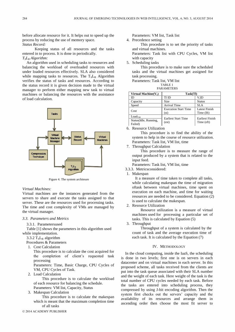
before allocate resource for it. It helps out to speed up the
process by reducing the use of memory space.
Status Record:
Keeping status of all resources and the tasks
entered in to process. It is done in periodically.
TSLB Algorithm:
An algorithm used in scheduling tasks to resources and
balancing the workload of overloaded resources with
under loaded resources effectively. SLA also considered
while mapping tasks to resources. The TSLB Algorithm
verifies the status of tasks and resources. According to
the status record it is given decision made to the virtual
manager to perform either mapping new task to virtual
machines or balancing the resources with the assistance
of load calculation.
Virtual Machines:
Virtual machines are the instances generated from the
servers to share and execute the tasks assigned to that
server. These are the resources used for processing tasks.
The time and cost complexity of VMs are managed by
the virtual manager.
3.3. Parameters and Metrics
3.3.1. Parametersused
Table [1] shows the parameters in this algorithm used
while implementation.
3.3.2 TSLB algorithm
Procedures & Parameters
1. Cost Calculation
This procedure is to calculate the cost acquired for
the completion of client‟s requested task
processing
Parameters: Time, Basic Charge, CPU Cycles of
VM, CPU Cycles of Task.
2. Load Calculation
This procedure is to calculate the workload
of each resource for balancing the schedule.
Parameters: VM list, Capacity, Status
3. Makespan Calculation
This procedure is to calculate the makespan
which is meant that the maximum completion time
of all tasks
Parameters: VM list, Task list
4. Precedence setting
This procedure is to set the priority of tasks
and virtual machines.
Parameters: Task list with CPU Cycles, VM list
with capacity
5. Scheduling tasks
This procedure is to make sure the scheduled
tasks and the virtual machines get assigned for
task processing.
Parameters: Task list, VM list TABLE 1
PARAMETERS
6. Resource Utilization
This procedure is to find the ability of the
system to help in the course of resource utilization.
Parameters: Task list, VM list, time
7. Throughput Calculation
This procedure is to measure the range of
output produced by a system that is related to the
input feed.
Parameters: Task list, VM list, time
3.3.3. Metricsconsidered:
1. Makespan
It a measure of time taken to complete all tasks,
while calculating makespan the time of migration
oftask between virtual machines, time spent on
execution on each machine, and time for waiting
resources are needed to be considered. Equation (2)
is used to calculate the makespan.
2. Resource Utilization
Resource utilization is a measure of virtual
machines used for processing a particular set of
tasks. This is calculated by Equation (5)
3. Throughput
Throughput of a system is calculated by the
count of task and the average execution time of
each task. It is calculated by the Equation (7)
IV. METHODOLOGY
In the cloud computing, inside the IaaS, the scheduling
is done in two levels; first one is on servers in each
datacenter and on virtual machines in each server. In this
proposed scheme, all tasks received from the clients are
put into the task queue associated with their SLA number
and the weight of each task. Here weight of the task is the
total number of CPU cycles needed by each task. Before
the tasks are entered into scheduling process, they
compressed by using J-bit encoding algorithm. Then the
system first checks out the servers‟ capacity and the
availability of its resources and arrange them in
ascending order then choose the most fit server to
Virtual Machine(Vr) Task(Tl)
ID Tl ID VrID
Capacity Size Status
Speed Arrival Time SLA
Cost Execution Start Time
(st)
Latest Finish
Time (lft)
LoadVM Earliest Start Time (est)
Earliest Finish Time (eft)
Status(Idle, Running,
Failed)
Figure 4. The system architeure
284 JOURNAL OF EMERGING TECHNOLOGIES IN WEB INTELLIGENCE, VOL. 6, NO. 3, AUGUST 2014
© 2014 ACADEMY PUBLISHER

4.1 Procedure of TSLB Algorithm
The simplest procedure of TSLB algorithm is shown
below:
1. Take compressed tasks and Virtual Machines are as
input
2. Initialize the status record
3. Set priority by „priority setting‟ procedure based on
CPU cycles.
4. Load of virtual machines calculated by „Load
Calculation‟ procedure
5. Update status record
6. Assign task to virtual machine by „Mapping‟
procedure.
Procedure Schedule (vr[],tl[]){
for each tl
for each vr
{ //get load of each virtual machine from load
calculation procedure
currentcapacity[vr]=capacity[vr]-load[vr]
//get task status from status record
If(load[vr]<=capacity[vr] &&
status[tl]==’waiting’
&&tcw[tl]<=currentcapacity[vr]
vrtcw[tl]}
} //output:virtual machines and their assigned
tasks
Procedure Load(vr[],tcw[],tcr[])
{
for each vr{
for each tcw,tcr}
Load[vr]=tc[tcw]+tc[tcr]}
}
} //output:load of each virtual machine
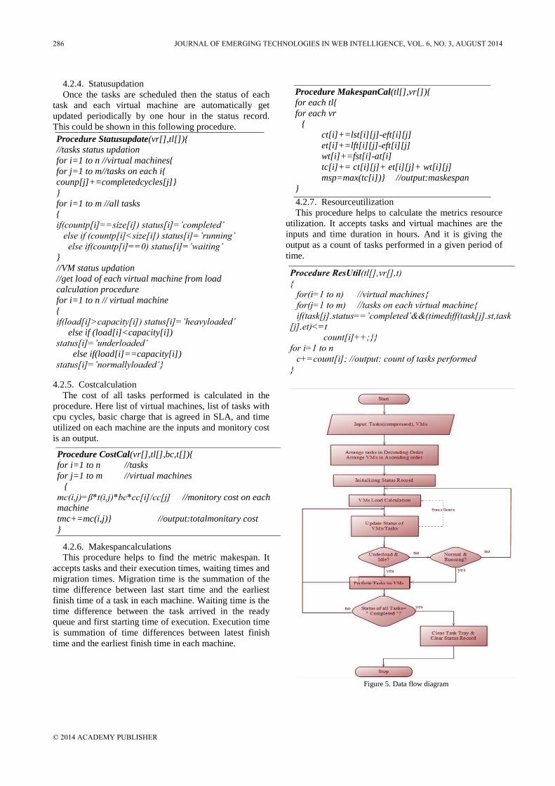
perform the given task list. After selecting the server the
process of TSLB will start. In Figure 5 the planning of the
data flow of TSLB algorithm is sketched clearly.
The detailed procedure of the TSLB algorithm is show
below:
4.2. Procedures and Pseudo Code:
This section revealed the list of pseudo codes of
procedures used on the TSLB algorithm and the pseudo
codes of metrics costing:
4.2.1 Precedence setting This procedure takes compressed tasks and their CPU
cycles needed and the resources and their capacity as
inputs. Next arrange all tasks in ascending order and all
resources in descending order. The outputs of this
procedure are the ordered tasks and resources.
4.2.2. Loadcalculation
Load of virtual machine is needed to calculate for
scheduling to avoid congestion. For that here the
procedure has taken the resource „vr‟ and all tasks‟ CPU
cycles in waiting queue „tcw‟ and in processing „tcr‟ are
as input and determines the load. According to the load of
each machine that is calculated, the status record gets
updated. So here the load of each virtual machine is the
output
4.2.3. Scheduling
This procedure handles assigning tasks, tl[], to virtual
machines, vr[], according to the load calculated by the
„Load‟ procedure. So here the compressed and ordered
tasks those are waiting for resources and the ordered
virtual machines those are ready to receive tasks for
processing are the inputs.
∀𝑉𝑀
∀ 𝑠𝑐ℎ𝑑𝑢𝑙𝑒𝑑 𝐶𝑇
1. Input: CTi(from TaskTray),VMj,tq; i=1…n|n≥1;
j=1…m|m≥1
2. ∀𝑉𝑀, ∀𝐶𝑇,
Call “PreSet”
3. ∀𝑉𝑀,
Call “Load”
4. ∀𝑉𝑀, ∀ 𝑢𝑛𝑠𝑐ℎ𝑑𝑢𝑙𝑒𝑑 𝐶𝑇,
If Curr.Cap[VMi]≤ Size[CTi] &&
Status[VMi]= „idle‟ || Status[VMi]=
„underloaded‟ then
Call “Schedule”
Call “Statusupdate”
5. 𝑖𝑓𝑡𝑞𝑡ℎ𝑒𝑛
If Status[CTi]==”WoM” &&
Status[VMi]== „overloaded‟ then
Move CTi to TaskTray
Else If Status[CTi]==”Completed”
then
Delete CTi from TaskTray
Call “Statusupdate”
6. Repeat 1 to 5 till
∀𝐶𝑇 , Status[CTi]==”Completed”||
∃𝐶𝑇 𝑜𝑛 𝑇𝑎𝑠𝑘𝑇𝑟𝑎𝑦
Procedure PreSet(tl[], vr[])
{
for each tl {
iftc[tl]>tc[tl+1] {
temp= tl;
tl = tl +1;
tl+1=temp; } }
for each vr {
if capacity[vr]<capacity[vr+1] {
Temp=vr;
vr=vr+1;
vr+1=temp; } }
} //output: ordered tasks and virtual machines
JOURNAL OF EMERGING TECHNOLOGIES IN WEB INTELLIGENCE, VOL. 6, NO. 3, AUGUST 2014 285
© 2014 ACADEMY PUBLISHER
Procedure CostCal(vr[],tl[],bc,t[]){
for i=1 to n //tasks
for j=1 to m //virtual machines
{
mc(i,j)=β*t(i,j)*bc*cc[i]/cc[j] //monitory cost on each
machine
tmc+=mc(i,j)} //output:totalmonitary cost
}
Procedure MakespanCal(tl[],vr[]){
for each tl{
for each vr
{
ct[i]+=lst[i][j]-eft[i][j]
et[i]+=lft[i][j]-eft[i][j]
wt[i]+=fst[i]-at[i]
tc[i]+= ct[i][j]+ et[i][j]+ wt[i][j]
msp=max(tc[i])} //output:maskespan
}
Procedure ResUtil(tl[],vr[],t)
{
for(i=1 to n) //virtual machines{
for(j=1 to m) //tasks on each virtual machine{
if(task[j].status==’completed’&&(timediff(task[j].st,task
[j].et)<=t
count[i]++;}}
for i=1 to n
c+=count[i]; //output: count of tasks performed
}
4.2.4. Statusupdation
Once the tasks are scheduled then the status of each
task and each virtual machine are automatically get
updated periodically by one hour in the status record.
This could be shown in this following procedure.
4.2.5. Costcalculation
The cost of all tasks performed is calculated in the
procedure. Here list of virtual machines, list of tasks with
cpu cycles, basic charge that is agreed in SLA, and time
utilized on each machine are the inputs and monitory cost
is an output.
4.2.6. Makespancalculations
This procedure helps to find the metric makespan. It
accepts tasks and their execution times, waiting times and
migration times. Migration time is the summation of the
time difference between last start time and the earliest
finish time of a task in each machine. Waiting time is the
time difference between the task arrived in the ready
queue and first starting time of execution. Execution time
is summation of time differences between latest finish
time and the earliest finish time in each machine.
4.2.7. Resourceutilization
This procedure helps to calculate the metrics resource
utilization. It accepts tasks and virtual machines are the
inputs and time duration in hours. And it is giving the
output as a count of tasks performed in a given period of
time.
Procedure Statusupdate(vr[],tl[]){
//tasks status updation
for i=1 to n //virtual machines{
for j=1 to m//tasks on each i{
counp[j]+=completedcycles[j]}
}
for i=1 to m //all tasks
{
if(countp[i]==size[i]) status[i]=‟completed‟
else if (countp[i]<size[i]) status[i]=‟running‟
else if(countp[i]==0) status[i]=‟waiting‟
}
//VM status updation
//get load of each virtual machine from load
calculation procedure
for i=1 to n // virtual machine
{
if(load[i]>capacity[i]) status[i]=‟heavyloaded‟
else if (load[i]<capacity[i])
status[i]=‟underloaded‟
else if(load[i]==capacity[i])
status[i]=‟normallyloaded‟}
}
Figure 5. Data flow diagram
286 JOURNAL OF EMERGING TECHNOLOGIES IN WEB INTELLIGENCE, VOL. 6, NO. 3, AUGUST 2014
© 2014 ACADEMY PUBLISHER
Procedure Thruput(tl[],vr[],t[]){
t1=ft[t1,v1]-st[t1,v1] //time taken to complete single
task
for(i=1 to n) //virtual machines
for(j=1 to m) //tasks
{
t2[i]+=ft[j]-st[j] //time taken to complete allotted
tasks on single machine
}
for(i=1 to n ) //all t2 s
t3+=t2[i] //time taken to complete all tasks
for(i=1 to n) //all task
aet[i]= (t1/t2[i])/t3
Tp=taskcount/MAX(aet[i])
}
4.2.8. Throughputcalculation:
This procedure facilitates to locate the metric named
through put. For that it accepts the tasks, virtual machines,
and execution details of each task on various machines
thenperforms the required calculation and utilizes the
equation and giving the throughput as an output.
V. IMPLEMENTATION
5.1. ExperimentalSetup:
The LBTS algorithm has been implemented in
Microsoft Visual Studio 2012 Express on Windows
Azure Platform. It provides the easiest way of virtual
machine creation and provides multiples of class libraries
for the .Net developers [13]. All those libraries can be
used by downloading NuGet package manager on
Microsoft Visual Studio 2012. NuGet is the package
manager with number of tools that facilitate the
constructing and deconstructing packages [14].
5.2. Variation on Inputs and Its Effects:
Firstly, make the flow of uncompressed tasks (files)
through this algorithm and collected the results to verify
the metrics. Next collect and verify the metrics values
with compressed tasks.
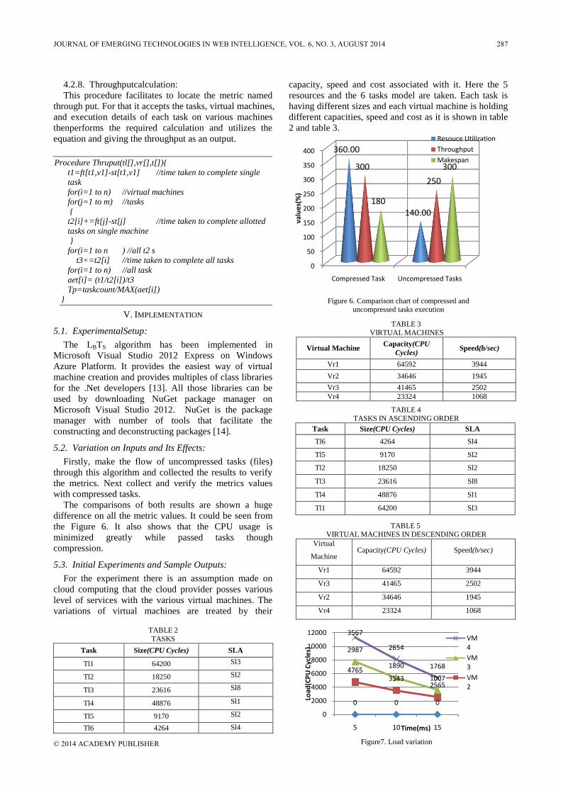
The comparisons of both results are shown a huge
difference on all the metric values. It could be seen from
the Figure 6. It also shows that the CPU usage is
minimized greatly while passed tasks though
compression.
5.3. Initial Experiments and Sample Outputs:
For the experiment there is an assumption made on
cloud computing that the cloud provider posses various
level of services with the various virtual machines. The
variations of virtual machines are treated by their
capacity, speed and cost associated with it. Here the 5
resources and the 6 tasks model are taken. Each task is
having different sizes and each virtual machine is holding
different capacities, speed and cost as it is shown in table
2 and table 3.
Figure 6. Comparison chart of compressed and
uncompressed tasks execution
0
50
100
150
200
250
300
350
400
Compressed Task Uncompressed Tasks
360.00
140.00
300
250
180
300
valu
es(
%)
Resouce Utilization
Throughput
Makespan
TABLE 2
TASKS
Task Size(CPU Cycles) SLA
Tl1 64200 Sl3
Tl2 18250 Sl2
Tl3 23616 Sl8
Tl4 48876 Sl1
Tl5 9170 Sl2
Tl6 4264 Sl4
TABLE 3 VIRTUAL MACHINES
Virtual Machine Capacity(CPU
Cycles) Speed(b/sec)
Vr1 64592 3944
Vr2 34646 1945
Vr3 41465 2502
Vr4 23324 1068
TABLE 4
TASKS IN ASCENDING ORDER
Task Size(CPU Cycles) SLA
Tl6 4264 Sl4
Tl5 9170 Sl2
Tl2 18250 Sl2
Tl3 23616 Sl8
Tl4 48876 Sl1
Tl1 64200 Sl3
TABLE 5
VIRTUAL MACHINES IN DESCENDING ORDER
Virtual
Machine Capacity(CPU Cycles) Speed(b/sec)
Vr1 64592 3944
Vr3 41465 2502
Vr2 34646 1945
Vr4 23324 1068
Figure7. Load variation
0 0 0
47653543
2565
2987
1890
1007
3567
2654
1768
0
2000
4000
6000
8000
10000
12000
5 10 15
Load
(CP
U C
ycle
s)
Time(ms)
VM4
VM3
VM2
JOURNAL OF EMERGING TECHNOLOGIES IN WEB INTELLIGENCE, VOL. 6, NO. 3, AUGUST 2014 287
© 2014 ACADEMY PUBLISHER

By calling the PreSet procedure the tasks and virtual
machines are arranged in ascending and descending order.
Table 4 and Table 5 show the result of PreSet procedure
calling.
Initially the status of tasks and virtual machines are
empty. Once the execution of task has been started on
virtual machines, then the values of status record gets
updated after the given period. The capacity of each
virtual machine also changed after starting task
processing. Here the variations are monitored on each
time quantum and updated in the status record. The table
6 shows filtered values from the status record that is
obtained with 30mins time quantum.
Experiments on metrics:
This section concise the values of various metrics
those are taken in account while structuring and
implementing the TSLB algorithm.
The load of each virtual machines obtained by the
procedure Load and the metric values Makespan,
Resource Utilization and Throughput are obtained in the
course of calling their corresponding procedures. The
graph in the Figure 7 shows the load variation of virtual
machines on few of its time quantum.
Resource utilization of an overall system is calculated
through the procedure ResUtil, is the implementation of
an equation (5). Here it is needed to know the difference
between the CPU usage and the resource utilization. This
paper means that CPU usage is the space occupied on a
memory by a task while processing. But resource
utilization is calculated based on the ability of handling
number of CPU Cycles by a virtual machine in a given
period of time. The graph illustrated in Figure 8 shows
the task handled ratio of each virtual machine.
The metric throughput values are collected by
implementing and executing the procedure „Thruput‟
which follows on equation (6).
Throughput means that here the expected ratio of
output in an average execution time of a set of task. The
graph in Figure 9 shows the throughput ratio of each
task.Makespan is calculated by calling the procedure
MakespanCalwhich holds the implementation of equation
(3) and the monitory cost is calculated by
CostCalprocedure.
For calculating monitory cost, the random number β
generated dynamically and measured cost afford for the
utilization of resources. The Figure 10 shows the
relativity of makespan and monitory cost by the values
given through the execution.
VI.RESULT ANALYSIS AND DISCUSSION
This section covers the comparison of overall
performance of the TSLB algorithm against the algorithms
in [2][3][5][6]. The main goal of this TSLB algorithm is to
maximizing the resource utilization by decreasing the
CPU usage of the resources. This was initially achieved
by using task compression [10]. Thus the discussion
hereabout the resource utilization of different algorithms
Figure 8. Resource utilization
050000
100000150000200000250000300000350000400000450000500000
100 150 200 250
CP
U C
ycle
s
Time/ms
VM1
VM2
VM3
VM4
Figure 9. Throughput
0
5
10
15
20
100 200 300 400 500 600
18.34
9.13 9.08
16.29
9.17
6.09
Thro
ugh
pu
t
Time(ms)
TABLE 6
STATUS RECORD
Virtual
Machines Tasks
Starting
Time Finish Time
CPU cycles
allotted
Status of
Tasks
Status of
VM
Capacity
of VM
Vr1 Tl6 11:00 11:02 4264 Completed Underload 60328
Vr3 Tl5 11:00 11:05 9170 Completed Underload 32295
Vr2 Tl2 11:01 11:19 18250 Completed Underload 16396
Vr4 Tl3 11:01 11:25 23324 Completed Normal 0
Vr1 Tl4 11:03 11:06 48876 Completed Underload 11451
Vr3 Tl1 11:06 11:20 32295 Completed Normal 0
Vr2 Tl3 11:20 11:27 291 Completed Underload 28250
Vr1 Tl1 11:26 11:30 9170 Completed Underload 1281
288 JOURNAL OF EMERGING TECHNOLOGIES IN WEB INTELLIGENCE, VOL. 6, NO. 3, AUGUST 2014
© 2014 ACADEMY PUBLISHER

thoseare revised in the background study section. Table 7
shows the comparison result of usage of resources by the
various scheduling schemes and the Figure 11 shows the
graphical presentation of the same. The TSLB algorithm is
executed with different sets of tasks and with different
capacity of virtual machines. Then those obtained values
are compared with the results produced by other
algorithms.
The comparative result shows that the TSLB algorithm
is produced good makespan than others. At every
quantum of time period the load of each resource are
calculated and reschedule them so the resources are not
falling in wastage of time and help to produce high
throughput than other algorithms. Graphs in Figure 12
and Figure 13 show the variation of throughput and
makespan, monitory cost of different algorithms.
VII.CONCLUSION
Load balancing is one of the researchable area in the
cloud computing and it could be more efficient when
using with scheduling. Here the cost efficient load
balancing scheme is introduced and the algorithm
introduced in it is called TSLB algorithm. Nowadays in the
cloud environment processing huge amount of data from
its more than billion customers is crucial due to the lack
of resources. So the foremost theme of this newly devised
algorithm is to reduce the usage of memory while
processing the tasks from its various clients. Through the
experiments it is also proved that this algorithm is
increasing the resource utilization, producing good
makespan and awarded high throughput. The
performance of this algorithm also compared with other
schemes and proved its effectiveness and the importance
in the cloud computing.
REFERENCES
[1] Barrie Sosinsky, Cloud Computing Bible(2011), Wiley
India Pvt Ltd.
[2] Sen Su, Cost-efficient task scheduling for executing large
programs in the cloud, SciVerseScienceDirect , Parallel
Computing 39 (2013) 177–188.
[3] Jose Luis Lucas-Simarro, “Scheduling strategies for
optimal service deployment across multiple clouds”,
SciVerseScienceDirect, Future Generation Computer
Systems 29 (2013) 1431–1441.
[4] Jinn-TsongTsai,“Optimized task scheduling and resource
allocation on cloud computing environment using
improved differential evolution algorithm”,
SciVerseScienceDirect, Computers & Operations Research
40 (2013)3045–3055".
[5] YuanjunLaili, “A Ranking Chaos Algorithm for dual
scheduling of cloud service and computing resource in
Figure10.Relativity of makespan and monitory cost
8
5
10
13
7
17
4.58
10
10.45
9.54
3.76
14.58
100
105
110
115
120
0.1 0.2 0.3 0.4 0.9 1
Tim
e/m
.sec
Cost
Makespan
Monitory Cost
Figure 12. Comparison result of makespan
1.52.09
32.5
2.031.45
3.87
2 1.78
1.042.34
2
11.5
1.002
1.01 1.006
0.08 0.05 0.030
1
2
3
4
5
Tl1 Tl2 Tl3 Tl4 Tl5
Mak
esp
an
Task set
POSHRanking ChaosDVFSTSLB
Figure 13. Comparison result of throughput
45.66
56.57
67.87
78.7985.67
34.45
45.56 47.4553.56
58.6532.3336.67
45.67 48.76
59.08
48.67
68.7977.88
87.9 90.86
0
20
40
60
80
100
100 200 300 400 500
Thro
ugh
pu
t(%
)
Time(m.sec)
POSH
Ranking Chaos
DVFS
TSLB
TABLE 7
COMPARATIVE RESULT OF RESOURCE UTILIZATION
Resources POSH Ranking
Chaos DVFS TSLB
V1 2.34 1.45 1.01 3.86
V2 1.24 1.35 1.04 2.01
V3 1.02 1.05 0.5 2.03
V4 1.75 1.83 1.06 2.01
Figure 11. Comparison result of resource utilization
0
1
2
3
4
Vr1 Vr2 Vr3 Vr4
2.34
1.24 1.021.75
1.45 1.351.05
1.831.01 1.04
0.51.06
3.86
2.012.03
2.01
Spac
e in
me
mo
ry
Resourceset
POSH
Ranking Chaos
DVFS
JOURNAL OF EMERGING TECHNOLOGIES IN WEB INTELLIGENCE, VOL. 6, NO. 3, AUGUST 2014 289
© 2014 ACADEMY PUBLISHER

private cloud”, SciVerseScienceDirect, Computers in
Industry, 64(2013)448–463.
[6] Chia-Ming Wu, “A green energy-efficient scheduling
algorithm using the DVFS technique for cloud datacenters”,
SciVerseScienceDirect, 2013, (article in press).
[7] Abraham Silberschatz, Peter Baer Galvin, Greg
Gagne,“Operating System Concepts”, Sixth Edition.
[8] PinalSalot, “A Survey of Various scheduling algorithm in
cloud omputing environment”, IRJET, vol.2, Is. 2, p.131-
135, yr.2013.
[9] Introduction to Data Compression, Guy E. Blelloch
[10] Capo-chichi, E. P., Guyennet, H. and Friedt, J. K-RLE a
“New Data Compression Algorithm for Wireless Sensor
Network”, In Proceedings of the 2009 Third International
Conference on Sensor Technologies and Applications.
[11] AgusDwiSuarjava, “A new algorithm for data compression
optimization”, IJACSA, vol.3, No.8, 2012.
[12] YatendraSahu, “Cloud Computing overview with load
balancing techniques”, International Journal of Computer
Applications, vol.65, No.24,p.0975-8887, 2013.
[13] Building Real-world Cloud Apps with Windows Azure,
Tom Dykstra Rick Anderson Mike Wasson, Microsoft
Corporation, January, 2014
[14] http://nuget.codeplex.com/documentation?title=Getting%2
0Started
[15] https://devcentral.f5.com/articles/intro-to-load-balancing-
for-developers-ndash-the-algorithms#.Us_xJprrbIU
[16] DhananjayM.Dhamdhere, Operating Systems-A Concept-
Based Approach
[17] Andrew S. Tanenbarem, Modern Operating System, 2nd
Edition
[18] Yiqiu Fang, Fei Wang, and Junwei, “A Task Scheduling
Algorithm Based on Load Balancing in Cloud Computing”,
Web Information Systems and Mining
[19] Lecture Notes in Computer science, vol 6318, pp 271-277,
2010.
SubasishMohapatra, Subhadarshini and K.SmrutiRekha,
“Analysis of Different Varients in Round Robin
Algorithms for Load Balancing in Cloud Computing”,
International Journal of Computer Applications, Vol.69,
No.22,pp 0975-8887, 2013.
[20] Canali C and Lancellotti R., “Improving Scalability of
Cloud Monitoring Through PCA - Based Clustering of
Virtual Machines”, Journal Of Computer Science And
Technology, 29(1), pp. 38-52,2014.
290 JOURNAL OF EMERGING TECHNOLOGIES IN WEB INTELLIGENCE, VOL. 6, NO. 3, AUGUST 2014
© 2014 ACADEMY PUBLISHER