Embed Size (px)
Citation preview
NASA/TP- 1998-208463
A Control Law Design Method Facilitating
Control Power, Robustness, Agility, and FlyingQualities Tradeoffs: CRAFT
Patrick C. Murphy and John B. Davidson
Langley Research Center, Hampton, Virginia
National Aeronautics and
Space Administration
Langley Research Center
Hampton, Virginia 23681-2199
September 1998

Available from the following:
NASA Center for AeroSpace Information (CASI)7121 Standard Drive
Hanover, MD 21076-1320
(301) 621-0390
National Technical Information Service (NTIS)
5285 Port RoyalRoad i ! _ - _)
Springfield, VA 22161-2171
(703) 487-4650
; I I|
Summary
Recent advances in aircraft technology are placing increasing demands on flight control designers tosatisfy many competing design objectives. Advances in weapons and aircraft technology are significantly
changing air combat for the next generation of fighter aircraft. New control effectors, such as thrust
vectoring, offer the capability to expand the flight envelope, but also complicate the control mix with
redundant effectors. Future fighters will operate in environments where having high levels of
maneuverability and controllability, throughout a greatly expanded flight envelope, are requirements.
These diverse and often competing requirements have created a need for a design method that allows
production of a balanced final design.
The control law design methodology outlined in this report enables a designer to integrate numerous
design requirements into one design process. This methodology, known as CRAFT, is named for the
design objectives addressed, namely, Control Power, Robustness, A__gility,and Flying Qualities Tradeoffs.
The approach combines eigenspace assignment with a graphical technique for representing numerous
design goals in one composite illustration. The design goals are represented by control design metrics
that are quantitative measures of specific system capabilities translating desired operational
characteristics into useful engineering terms for control design. The methodology described in this report
makes use of control design metrics from the four design objective areas indicated. Although these
metrics are key in control law design for fighter aircraft, the methodology is more broadly applicable and
any metric quantifying design requirements can be used; for example, metrics characterizing ride quality,
weapons control, or structural requirements may be key in certain designs.
The CRAFT methodology is demonstrated using a model of an experimental high performance F/A-18
fighter aircraft with thrust vectoring. Redundant control surfaces have been reduced to two orthogonal
control inputs (stability axis roll and yaw commands) by using the Pseudo Control method. Control
synthesis is accomplished using Direct Eigenspace Assignment (DEA). The DEA control synthesis
technique provides a mechanism to determine measurement feedback control gains that produce anachievable eigenspace for the closed-loop system.
In the CRAFT design process, the desired eigenspace is systematically varied over the complex plane,allowing the computation of metric values corresponding to each eigenspace specification. Metric values
are numerical representations of design criteria. Metric surfaces are formed by plotting metric values
corresponding to each frequency and damping point specified as a target eigenvalue. Graphical overlays
of the metric surfaces are then used to show the best design compromise. Because the sensitivity of the
metrics to pole placement is clearly displayed through surface gradients, the designer can readily assess
the cost of tradeoffs among many metrics. This approach enhances the designer's ability to make
informed design tradeoffs and to achieve effective final designs.
Introduction
Recent advances in aircraft technology are placing increasing demands on flight control design.
Lighter structure for increased performance or less structure for low radar cross-section, the need for good
flying qualities in extreme flight conditions, such as high angle-of-attack flight, demands for greater high-
speed performance and for lower cost have all increased the complexity of the flight control design
problem. Superimposed on these requirements, fighter aircraft have additional demands for agility, orenhanced maneuverability and controllability, resulting from advances in "point and shoot" weapons that
are significantly changing air combat for the next generation of fighter aircraft. In the past, air combat
engagements often resulted in tail-chase fights measured in minutes. Now engagements are measured in
secondswithcombatantsusingall-aspectweapons.Future fighters may have to operate in environments
where having substantial agility throughout a greatly expanded flight envelope is a requirement. Studies
involving piloted and numerical air combat simulations (refs. 1-6) have shown that fighters with this
capability are able to perform combat maneuvers in shorter time and in less space and thus achieve a
tactical advantage. The demand for agility adds complexity to the control design problem. In addition,new control effectors, such as thrust vectoring and actuated nose strakes, offer the capability to achieve
higher levels of agility than previously attainable, thus further complicating the control mix with
redundant effectors that have varying effectiveness over the flight envelope.
Research efforts have focused on characterizing an aircraft's agility and defining high angle-of-attack
flying qualities requirements. Many agility metrics have been proposed (refs. 7-14) for assessing combat
capability, but they do not readily lend themselves for use in the control design process. Efforts to
provide metrics for control law design have been reported in references 15-18 and have resulted in
candidate design metrics and guidelines that have proven useful to a flight control law designer. Inaddition, several related studies have been performed as part of the NASA High Alpha Technology
Program (HATP) (refs. 19-22). To achieve high levels of agility, including post-stall maneuvering
capability, successful development and integration of several emerging technologies, such as thrust
vectoring and highly integrated flight control systems, are required (ref. 23).
Successful completion of a control law design for systems incorporating these advanced capabilities
requires control design methods that handle diverse design requirements. These design methods mustallow the designer to conduct systematic tradeoffs to achieve a balanced design. This report describes a
design methodology that uses a graphical approach to achieve a balanced design for systems where the
design requirements can be quantified in the form of control design metrics. Control design metrics are
quantitative measures of specific system capabilities that translate desired operational characteristics intouseful engineering terms for control design. The design approach, referred to as CRAFT, stands for the
design objectives addressed, namely, C_ontrol Power, R_obustness, Agility, and _Flying Qualities T_radeoffs.
This approach, initially reported in reference 24, has been further developed and flight tested by
application to the NASA High Alpha Research Vehicle (HARV). HARV is an experimental F/A-18 that
uses both thrust vectoring and actuated nose strakes for enhanced high alpha control. This vehicle has a
programmable flight computer on board that allows testing of different research control laws.
For the HARV flight experiments, feedback gains were designed for both the NASA-1A and the
ANSER (Actuated Nose Strakes for Enhanced Rolling) control laws. For these flight experiments, alateral-directional control law was developed using CRAFT in combination with Pseudo Controls
(ref. 25). Pseudo Controls is a nonlinear control blending scheme that provides cooperative action amongredundant controls while minimizing the number of feedback gains required and the complication of
feedback gain schedules. Redundant control surfaces are reduced to two orthogonal control inputs by
using the Pseudo Control method. Within the CRAFT feedback design process, the Pseudo Control
system is linearized at design points to provide a linear matrix mapping between aircraft controls and the
two orthogonal pseudo controls. A description of one control law, labeled NASA-1A, providing botharchitecture and simulation results, can be found in reference 26. This control law was used in the HARV
thrust-vectoring-only experiments. A complete and detailed design specification for the ANSER control
law, which included both thrust-vectoring and actuated nose strakes, is provided in reference 27.
The CRAFT methodology provides a coherent design process allowing the designer to judge the
inevitable compromise among many different and often competing requirements. The process allows
optimization of aircraft agility, manual control requirements, system tolerance to model error, and
disturbance rejection, while at the same time respecting the limitations of finite control power.
I t i

Symbols and Abbreviations
aj
A
An
bj
B
Bn
C
CL_
Cn
D
E
g
gm
G
Gx
I
J
K
KG
L
L'p
L'_
L' 8
m
M
n
N
denominator coefficients for observer-canonical form
plant matrix
plant matrix for nonphysical states
numerator coefficients for observer-canonical form
control distribution matrix for states
control distribution matrix for nonphysical states
state distribution matrix for outputs
nondimensional variation of lift coefficient with angle of attack
state distribution matrix for nonphysical outputs
control distribution matrix for outputs
uncertainty model
feedback gain
gain metric based on sum of squares of gains
feedback gain matrix
maps states to controls, Gx = Jim - G Nc] -1 G M
identity matrix (subscripts indicate dimension)
complex number (j = xfL-1)
plant compensation
loop transfer matrix
matrix defining achievable subspace for v
roll moment due to roll rate, sec -1
roll moment due to sideslip angle, sec -2
roll moment due to control input, sec -2
number of controls
state distribution matrix for measurements
number of states
control distribution matrix for measurements

NPr
N'I3
N'_
P
Pstab
q
Qdi
r
rad
rstab
R n
S
T
Te2
U
U
v
V
Vo
W
W
X
Xn
Y
Y'_
Y'_
Z
yaw moment due to yaw rate, sec -1
yaw moment due to sideslip angle, sec -2
yaw moment due to control input, sec -2
number of outputs
stability-axis roll rate, rad/sec
number of eigenvector elements specified
weighting matrix to select elements of desired eigenvector
number of measurements
radians
stability-axis yaw rate, rad/sec
vector space of dimension n
Laplace variable, s = j co
scale matrix
flight path attitude lag parameter, sec
single control input
control vector (m x 1)
side velocity, ft/sec
matrix of eigenvectors
trim velocity, ft/sec
desired eigenvector projection vector
matrix of wi columns
state vector (n x 1)
nonphysical state vector
output vector (p x 1)
side force due to sideslip angle, sec -1
side force due to control input, sec -1
measurement vector (r x 1)
angle of attack, rad
4

13 sideslip, rad
_5 generic control input
A transfer function denominator
damping ratio
0 pitch angle, rad
_, eigenvalue
_roll roll mode eigenvalue
v eigenvector
t_ minimum singular value
maximum singular value
_)stab stability axis bank angle, rad
¢o frequency, rad/sec
element of set
Subscripts
a achievable values
c associated with controller
DR Dutch roll
d desired values
i index over n modes
p associated with pilot
s scaled vector or matrix
ss steady state
Superscripts
p number of outputs
T matrix transpose
Abbreviations
AOA angle of attack, rad
CO combat
CRAFT
DEA
HARV
HATP
Mil-Std
MIMO
rad
RMS
sec
SISO
SSV
Control Power Robustness _Agility and _Flying Qualities Tradeoffs
Direct Eigenspace Assignment
High Alpha Research Vehicle
High Alpha Technology Project
Military Standard Specifications
multiple input, multiple output system
radians
root mean square
seconds
single input, single output system
structured singular value
Control Design Metrics
Mag
Mcp
Mdr
Mri
Mro
agility metric for yawing motion
control power metric, defined as RMS magnitude of feedback gains
flying qualities metric for Dutch roll mode
robustness metric for uncertainty at the inputs
robustness metric for uncertainty at the outputs
CRAFT Design Method
CRAFT is a control law design approach that addresses key design objectives of concern to many
flight control designers, namely, tradeoffs among control power, robustness, agility, and flying qualitiesrequirements. This approach provides the designer with a graphical tool to simultaneously assess any
quantifiable metric representing design objectives. The strength of this approach cornes from thecombined use of eigenspace assignment, which allows direct specification of eigenvalues and
eigenvectors in the design, and graphical overlays of metric surfaces that capture the design goals in a
composite illustration. Although eigenspace assignment facilitates this design process very efficiently, a
number of design methods can be used to determine feedback gains in this approach. Designers must
choose a control design algorithm and appropriate design metrics suited for each design problem.
In the CRAFT approach, design tradeoffs are made by interpreting graphical overlays of metric
surfaces that quantitatively characterize each design goal. Numerous metrics from each of the key design
objective areas can be applied simultaneously. Any unique metric reflecting a specialized requirement
that can be expressed in engineering terms can be applied as well. Graphical overlays of the metric
surfaces show the best design compromise for all the design criteria and clearly display the sensitivity of
changing from that best-compromise design point. This feature can greatly enhance the designer's ability
to make informed design tradeoffs.
6
I II1
Method Overview .....
CRAFT is summarized in block diagram form in figure 1. The design process begins by selecting a
reasonable range of frequency and damping for the closed-loop dynamics of interest. For example, if a
longitudinal design was desired, a range of frequency and damping for the short-period mode would be
selected with the phugoid mode specified to meet Level 1 flying qualities. Within this range, a grid ofdesign points is chosen to systematically cover the design space. Using eigenspace assignment as the
control design algorithm, feedback gains are computed to achieve the desired dynamics for the closed-
loop system at each design point. With eigenspace assignment, the designer must define both eigenvaluesand eigenvectors; specifying the eigenvectors is discussed in sections "Eigenspace Selection" and
"Design Issues." Once the desired closed-loop systems are determined for a specified set of frequency
(to) and damping ratio (4) pairs, each control design metric can be evaluated and plotted, producing asurface over the k-to space. Some metrics, such as flying qualities specifications, may be known before
the closed-loop design; however, the control power, robustness, and agility metrics require determination
of the closed-loop system. Viewing the metric surface in a 2-D contour plot highlights the most desirable
region to locate the short period pole with respect to the particular metric studied. The individual metric
surfaces are an indication of the sensitivity of that metric to closed-loop pole location. A final overlayplot of desirable regions from each metric surface can then be obtained. This is represented by the
bottom center block of figure 1. The intersection of desirable regions provides the best designcompromise for all the design criteria considered.
One possible result of applying the CRAFT method is that some of the most desirable regions do not
overlap. In such a case, a solution for all the metrics to be satisfied simultaneously does not exist, and
therefore some compromise will be required. For example, the designer may feel it is better to give up
Level 1 flying qualities to achieve acceptable robustness margins, or agility might be reduced to maintain
acceptable flying qualities. With graphical overlays of metric surfaces, the designer is given a clear
picture of both the sensitivities and impact of the tradeoffs being made. Although many metrics can beused, the designer can weight certain design metrics to achieve a desired final effect.
Control Synthesis Algorithm
In this study, the control synthesis algorithm is Direct Eigenspace Assignment (DEA), taken fromreference 28. This control synthesis technique provides a mechanism to determine measurement
feedback control gains that produce an achievable eigenspace for the closed-loop system. It has been
shown (ref. 29) that, for a system that is observable and controllable with n states, m controls, and r
measurements, one can exactly place r eigenvalues and m elements of their associated eigenvectors in the
closed-loop system. DEA provides a mechanism to find achievable eigenvectors by placing q dements
(m < q < n) of r eigenvectors associated with r eigenvalues through a least squares fit of the desiredeigenvectors to the achievable eigenspace.
Consider the observable and controllable system expressed as
)( = A X + Bc Uc + Bp Up (X e Rn) (1)
Y = C X + Dc Uc + Dp Up (Y e RP) (2)
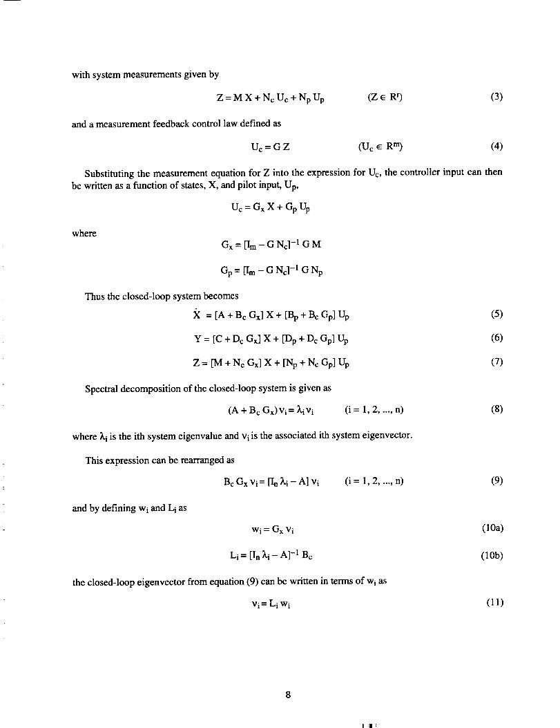
withsystemmeasurementsgivenby
Z=MX+NcUc +NpUp
andameasurementfeedbackcontrollawdefinedas
Uc=GZ
(Z e Rr) (3)
(Uc e Rm) (4)
Substituting the measurement equation for Z into the expression for Uc, the controller input can then
be written as a function of states, X, and pilot input, Up,
Uc= GxX + GpUp
(5)
(6)
(7)
(8)
(9)
(10a)
(10b)
(11)
where
Gx= [Im- G Nc] -1GM
Gp= lira -GNc] -1GNp
Thus the closed-loop system becomes
_( = [A + Bc Gx] X + [Bp + Bc Gp] Up
Y = [C + Dc Gx] X + [Dp + Dc Gp] Up
Z= [M +Nc Gx] X+ [Np +Nc Gp] Up
Spectral decomposition of the closed-loop system is given as
(A + B c Gx)V i= _vi (i = 1, 2..... n)
where _-i is the ith system eigenvalue and vi is the associated ith system eigenvector.
This expression can be rearranged as
Bc Gx Vi = [In _,i -- A] vi (i = 1, 2, ..., n)
and by defining wi and Li as
wi = Gx vi
Li = [In _ - A] -1 Bc
the closed-loop eigenvector from equation (9) can be written in terms of wi as
vi = Li wi
I II 1
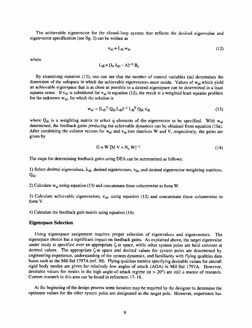
The achievable eigenvector for the closed-loop system that reflects the desired eigenvalue andeigenvector specification (see fig. 2) can be written as
Vai -- Ldi Wai (12)
where
Ldi = [In _qli- A] -1 Bc
By examining equation (12), one can see that the number of control variables (m) determines the
dimension of the subspace in which the achievable eigenvectors must reside. Values of Wai which yield
an achievable eigenspace that is as close as possible to a desired eigenspace can be determined in a least
squares sense. IfVdi is substituted for Vai in equation (12), the result is a weighted least squares problemfor the unknown Wai, for which the solution is
Wai = [LdiT Qdi Ldi] -1 LdiT Qdi Vdi (13)
where Qdi is a weighting matrix to select q elements of the eigenvector to be specified. With Wai
determined, the feedback gains producing the achievable dynamics can be obtained from equation (10a).
After combining the column vectors for Wai and Vai into matrices W and V, respectively, the gains aregiven by
G=W [M V +NcW] -1 (14)
The steps for determining feedback gains using DEA can be summarized as follows:
1) Select desired eigenvalues, Xdi, desired eigenvectors, Vdi, and desired eigenvector weighting matrices,Qdi.
2) Calculate Wai using equation (13) and concatenate these columnwise to form W.
3) Calculate achievable eigenvectors, Vai, using equation (12) and concatenate these columnwise toform V.
4) Calculate the feedback gain matrix using equation (14).
Eigenspace Selection
Using eigenspace assignment requires proper selection of eigenvalues and eigenvectors. The
eigenspace choice has a significant impact on feedback gains. As explained above, the target eigenvalue
under study is specified over an appropriate _-to space, while other system poles are held constant at
desired values. The appropriate _-t0 space and desired values for system poles are determined by
engineering experience, understanding of the system dynamics, and familiarity with flying qualities data
bases such as the Mil-Std 1797A (ref. 30). Flying qualities metrics specifying desirable values for aircraftrigid body modes are given for relatively low angles: of attack (AOA) in Mil-Std 1797A. However,
desirable values for modes in the high angle-of-attack regime (or > 20 °) are still a matter of research.Current research in this area can be found in references 17-18.
At the beginning of the design process some iteration may be required by the designer to determine the
optimum values for the other system poles not designated as the target pole. However, experience has
shownthatthis issueiseasyto resolve,especiallyif thereis sufficientfrequencyseparationbetweenthetargetpoleandothersystempoles.Nominalvaluesfor slowdynamics,suchasphugoidorspiralmodes,usuallycanbespecifiedoncewith little effectonthebestchoicefor thefastermodes.A slowmodecanbeoptimizedquicklyby designatingit asthetargetpolefor oneiterationin theCRAFTprocess,ifnecessary.
Eigenvectors,on theotherhand,needto be determined by the designer, and unfortunately, little
guidance is available for determining the best eigenvectors. Although Mil-Std 1797A does not provide
explicit guidance in the form of standard eigenvector specifications, it does provide a substantial body of
design criteria which describes desirable classical dynamics for aircraft transfer functions. This data base,
along with engineering experience, allows creation of design or "desired" eigenvectors. Mil-Std 1797A
captures a long history of experience with aircraft and specifies desirable aircraft dynamics mostly in low
order equivalent transfer function form. Transfer functions can be transformed to state-space form and
thus can define the eigenspace. Unfortunately, until more experience is obtained with aircraft capable of
high AOA, the Mil-Std for aircraft flying qualities is limited to providing low AOA design criteria.
However, for defining eigenvectors, other options exist besides building up a "desired" state-space model
from design criteria. The following sections introduce a few methods for specifying eigenvectors thathave been used with the CRAFT method. These methods are categorized as (1) open-loop eigenvectors,
(2) minimum-specification eigenvectors, and (3) desired-model eigenvectors. Results indicating some of
the advantages and disadvantages for these different approaches are discussed in "Design Issues."
Open-Loop Eigenvectors
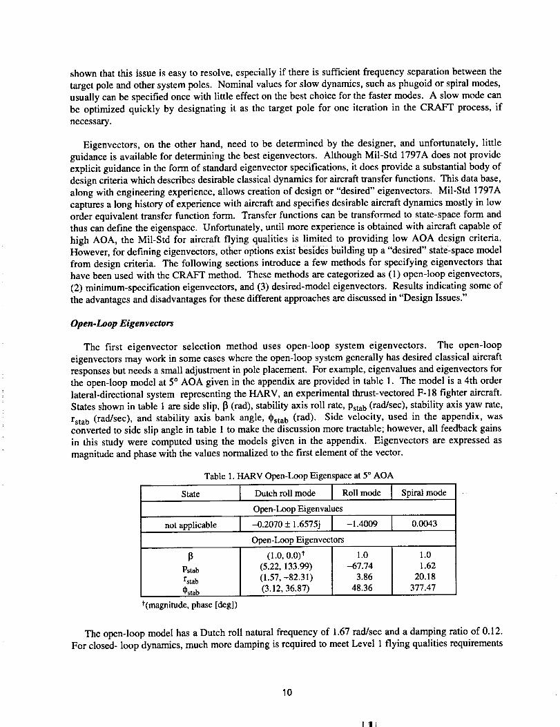
The first eigenvector selection method uses open-loop system eigenvectors. The open-loop
eigenvectors may work in some cases where the open-loop system generally has desired classical aircraft
responses but needs a small adjustment in pole placement. For example, eigenvalues and eigenvectors forthe open-loop model at 5° AOA given in the appendix are provided in table 1. The model is a 4th order
lateral-directional system representing the HARV, an experimental thrust-vectored F-18 fighter aircraft.
States shown in table 1 are side slip, [3 (rad), stability axis roll rate, Pstab (rad/sec), stability axis yaw rate,
rstab (rad/sec), and stability axis bank angle, t_stab (rad). Side velocity, used in the appendix, wasconverted to side slip angle in table 1 to make the discussion more tractable; however, all feedback gains
in this study were computed using the models given in the appendix. Eigenvectors are expressed as
magnitude and phase with the values normalized to the first element of the vector.
Table 1. HARV Open-Loop Eigenspace at 5 ° AOA
State Dutch roll mode Roll mode Spiral mode, ,,. ,,,.
Open-Loop Eigenvalues
not applicable -0.2070 + 1.6575j -1.4009 0.0043
Open-Loop Eigenvectors
[3 (1.0, 0.0) t
Pstab (5.22, 133.99)rstab (1.57, -82.31)Cstab (3.12, 36.87)
*(magnitude, phase [deg])
1.0-67.74
3.8648.36
1.01.62
20.18377.47
The open-loop model has a Dutch roll natural frequency of 1.67 rad/sec and a damping ratio of 0.12.For closed- loop dynamics, much more damping is required to meet Level 1 flying qualities requirements
10
iii
for fighteraircraftin combatmaneuvering(ClassIV aircraft,COphase).TheDutchroll dampingratiomustbegreaterthan0.4andthenaturalfrequencymustbegreaterthan1.0rad/sec.Thisrepresentsacasewhereaviabledesigncouldbemadeusingopen-loopeigenvectorsandsimplycompensatingfor alackof Dutchroll damping.Theeigenvectorsshowafairly classicalanddesirablecharacter,becausetheroll modeisdominatedbyroll ratewithverylittle sideslip,andtheDutchroll modehasadesirablet_/_
ratio of about 3.0 (ref. 30). Thus, a designer could use these eigenvectors in a design specification with
the appropriate eigenvalues specified. An advantage of this approach is a straight-forward design process
and possibly very low feedback gains if the poles are not specified too far from the open-loop values.
Minimum-Specification Eigenvectors
The second eigenvector selection method is a straight forward technique that uses eigenvectors
defined by zeroes and ones. Each element of the eigenvector is chosen to be 0 or 1, as appropriate, to
achieve desired decoupling of the aircraft rigid body modes and to maintain linear independence of the
eigenvectors. For a design using the lateral-directional model in the appendix, the choice would reflect
the desire to decouple roll and Dutch roll modes. Specifying O's or l's in the "desired" eigenvector can
be done with eigenspace assignment, since the method will provide the closest achievable eigenvector to
that "desired" eigenvector. Minimum-specification eigenvectors have been used with success by Shapiro
and others in application to flight control design (refs. 31, 32). In references 26 and 27, this design
approach was used effectively for lateral-directional design of eigenvectors, but with modification, to
provide appropriate f/13 ratio over the CRAFT design space and to minimize gain magnitudes.
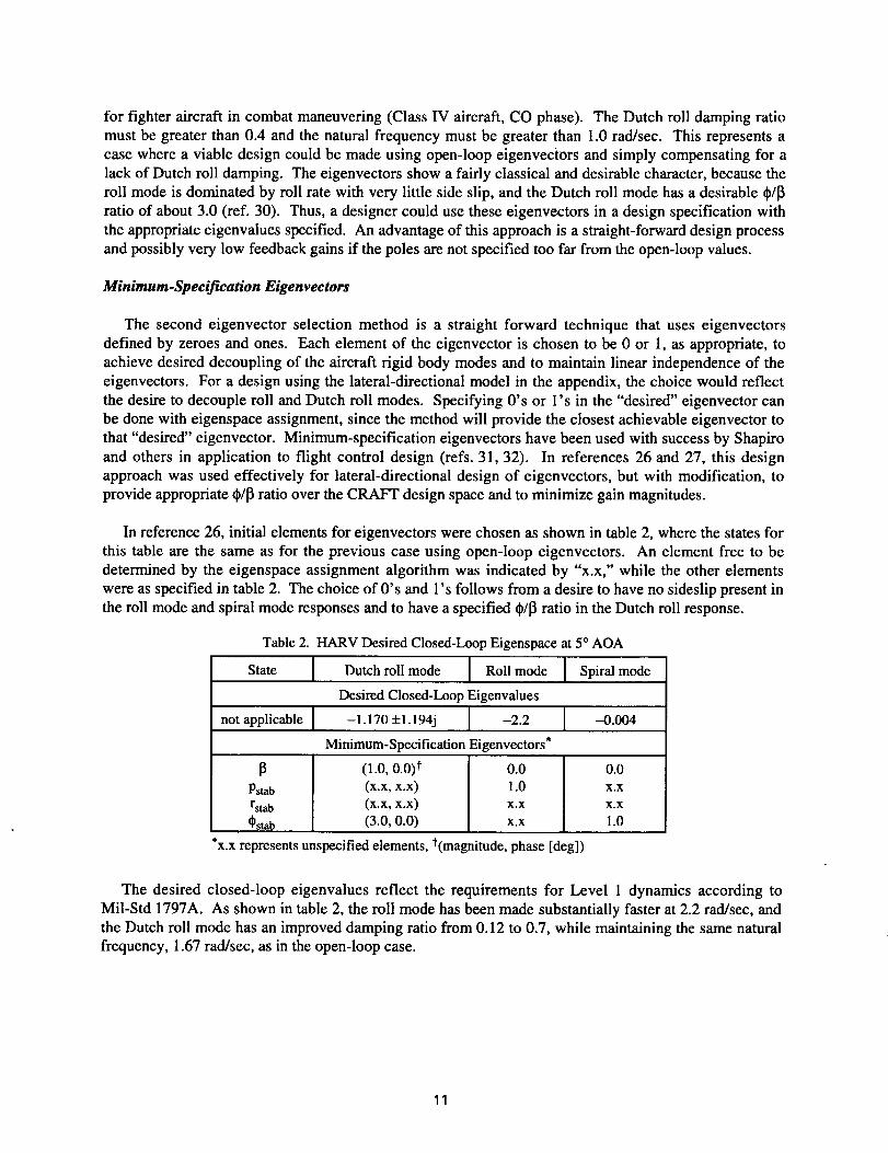
In reference 26, initial elements for eigenvectors were chosen as shown in table 2, where the states for
this table are the same as for the previous case using open-loop eigenvectors. An element free to be
determined by the eigenspace assignment algorithm was indicated by "x.x," while the other elements
were as specified in table 2. The choice of O's and 1's follows from a desire to have no sideslip present in
the roll mode and spiral mode responses and to have a specified t_/13ratio in the Dutch roll response.
Table 2. HARV Desired Closed-Loop Eigenspace at 5 ° AOA
State Dutch roll mode Roll mode Spiral mode
Desired Closed-Loop Eigenvalues
not applicable -1.170 + 1.194j -2.2 --0.004
Minimum-Specification Eigenvectors*
[3 (1.0, 0.0)* 0.0 0.0
Pstab (x.x, x.x) 1.0 x.xrstab (x.x, x.x) x.x x.xCstab (3.0, 0.0) x.x 1.0
x.x represents unspecified elements, t(magnitude, phase [deg])
The desired closed-loop eigenvalues reflect the requirements for Level 1 dynamics according to
Mil-Std 1797A. As shown in table 2, the roll mode has been made substantially faster at 2.2 rad/sec, andthe Dutch roll mode has an improved damping ratio from 0.12 to 0.7, while maintaining the same natural
frequency, 1.67 rad/sec, as in the open-loop case.
11
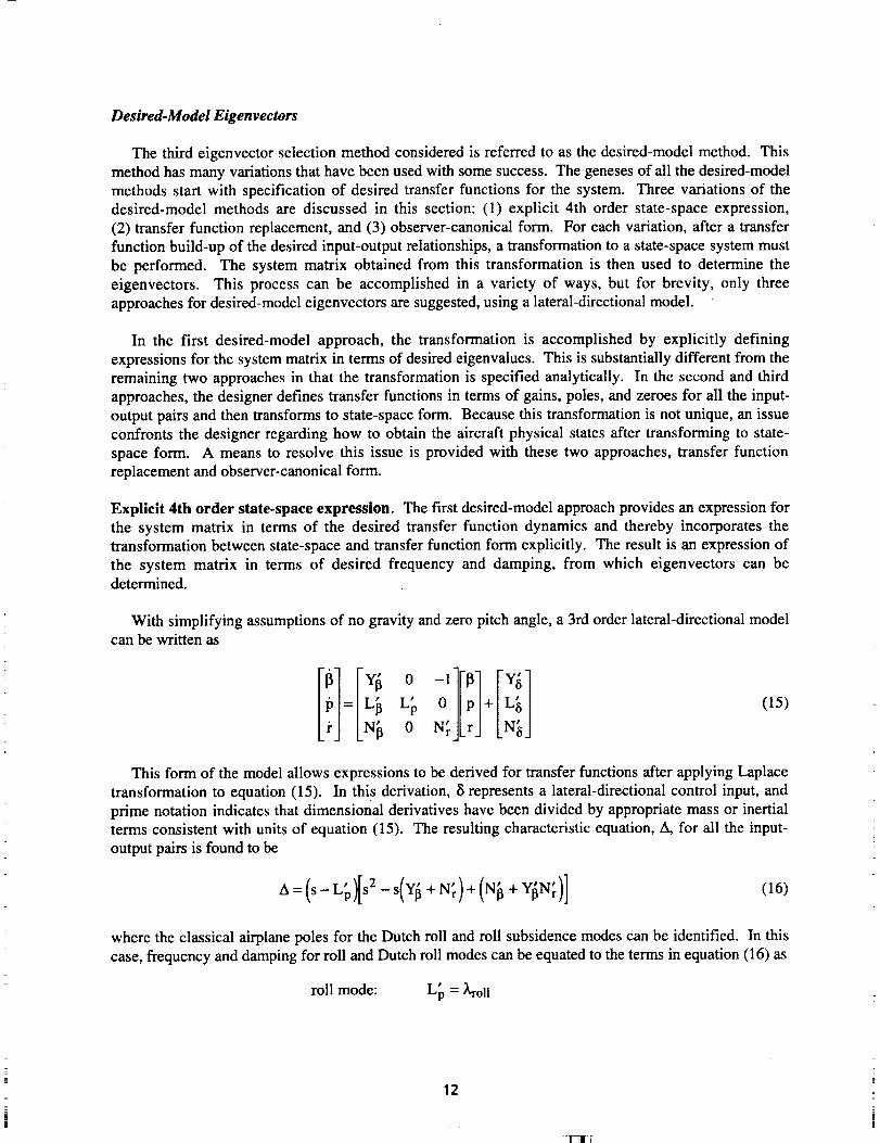
Desired-Model Eigenvectors
The third eigenvector selection method considered is referred to as the desired-model method. This
method has many variations that have been used with some success. The geneses of all the desired-model
methods start with specification of desired transfer functions for the system. Three variations of thedesired-model methods are discussed in this section: (1) explicit 4th order state-space expression,
(2) transfer function replacement, and (3) observer-canonical form. For each variation, after a transfer
function build-up of the desired input-output relationships, a transformation to a state-space system must
be performed. The system matrix obtained from this transformation is then used to determine the
eigenvectors. This process can be accomplished in a variety of ways, but for brevity, only three
approaches for desired-model eigenvectors are suggested, using a lateral-directional model.
In the first desired-model approach, the transformation is accomplished by explicitly defining
expressions for the system matrix in terms of desired eigenvalues. This is substantially different from the
remaining two approaches in that the transformation is specified analytically. In the second and third
approaches, the designer defines transfer functions in terms of gains, poles, and zeroes for all the input-
output pairs and then transforms to state-space form. Because this transformation is not unique, an issue
confronts the designer regarding how to obtain the aircraft physical states after transforming to state-
space form. A means to resolve this issue is provided with these two approaches, transfer functionreplacement and observer-canonical form.
Explicit 4th order state-space expression. The first desired-model approach provides an expression for
the system matrix in terms of the desired transfer function dynamics and thereby incorporates the
transformation between state-space and transfer function form explicitly. The result is an expression of
the system matrix in terms of desired frequency and damping, from which eigenvectors can bedetermined.
With simplifying assumptions of no gravity and zero pitch angle, a 3rd order lateral-directional modelcan be written as
: +IL IN_ 0 N;JLrj LN_J
(15)
This form of the model allows expressions to be derived for transfer functions after applying Laplace
transformation to equation (15). In this derivation, 8 represents a lateral-directional control input, and
prime notation indicates that dimensional derivatives have been divided by appropriate mass or inertial
terms consistent with units of equation (15). The resulting characteristic equation, A, for all the input-
output pairs is found to be
.,,_-(s- )[,,_ +N;)-,--,- )] (16)
where the classical airplane poles for the Dutch roll and roll subsidence modes can be identified. In this
case, frequency and damping for roll and Dutch roll modes can be equated to the terms in equation (16) as
t
roll mode: Lp = _,roll
12
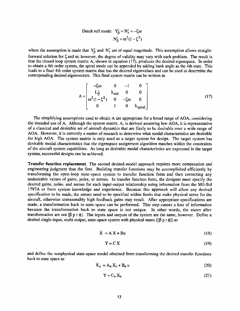
Dutchroll mode: Y6 = Nr = -_o_
= c02(1-42)
where the assumption is made that Y6 and N r are of equal magnitude. This assumption allows straight-
forward solution for _ and co; however, the degree of validity may vary with each problem. The result isthat the closed-loop system matrix A, shown in equation (17), produces the desired eigenspace. In orderto obtain a 4th order system, the spiral mode can be appended by adding bank angle as the 4th state. Thisleads to a final 4th order system matrix that has the desired eigenvalues and can be used to determine thecorresponding desired eigenvectors. This final system matrix can be written as
-_; 0 -1 0 1A = [O2(10 _2 ) _'roll 0
0 -_to _ (17)
1 0 Z,spiral
The simplifying assumptions used to obtain A are appropriate for a broad range of AOA, considering
the intended use of A. Although the system matrix, A, is derived assuming low AOA, it is representative
of a classical and desirable set of aircraft dynamics that are likely to be desirable over a wide range of
AOA. However, it is currently a matter of research to determine what modal characteristics are desirable
for high AOA. The system matrix is only used as a target system for design. The target system has
desirable modal characteristics that the eigenspace assignment algorithm matches within the constraints
of the aircraft system capabilities. As long as desirable modal characteristics are expressed in the target
system, successful designs can be achieved.
Transfer function replacement. The second desired-model approach requires more computation and
engineering judgment than the first. Building transfer functions may be accomplished efficiently by
transforming the open-loop state-space system to transfer function form and then correcting any
undesirable values of gains, poles, or zeroes. In transfer function form, the designer must specify the
desired gains, poles, and zeroes for each input-output relationship using information from the Mil-Std1797A or from system knowledge and experience. Because this approach will allow any desired
specification to be made, the zeroes need to be specified within limits that make physical sense for the
aircraft, otherwise unreasonably high feedback gains may result. After appropriate specifications are
made, a transformation back to state space can be performed. This step causes a loss of information
because the transformation back to state space is not unique. In other words, the states after
transformation are not [_ p r _p]. The inputs and outputs of the system are the same, however. Define a
desired single-input, multi-output, state-space system with physical states ([13 p r 4]) as
_( =AX+Bu (18)
Y = C X (19)
and define the nonphysical state-space model obtained from transforming the desired transfer functions
back to state space as
Xn = An Xn + Bn u (20)
Y=CnXn (21)
13
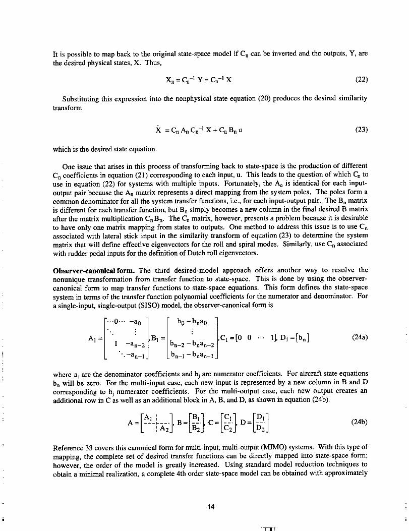
It is possible to map back to the original state-space model if C n can be inverted and the outputs, Y, are
the desired physical states, X. Thus,
Xn = Cn-1 Y = Cn-1 X (22)
Substituting this expression into the nonphysical state equation (20) produces the desired similaritytransform
_[ = Cn An Cn-1X + Cn Bn u (23)
which is the desired state equation.
One issue that arises in this process of transforming back to state-space is the production of different
Cn coefficients in equation (21) corresponding to each input, u. This leads to the question of which Cn to
use in equation (22) for systems with multiple inputs. Fortunately, the A n is identical for each input-
output pair because the An matrix represents a direct mapping from the system poles. The poles form a
common denominator for all the system transfer functions, i.e., for each input-output pair. The Bn matrix
is different for each transfer function, but Bn simply becomes a new column in the final desired B matrix
after the matrix multiplication Cn Bn. The Cn matrix, however, presents a problem because it is desirable
to have only one matrix mapping from states to outputs. One method to address this issue is to use Cn
associated with lateral stick input in the similarity transform of equation (23) to determine the system
matrix that will define effective eigenvectors for the roll and spiral modes. Similarly, use Cn associated
with rudder pedal inputs for the definition of Dutch roll eigenvectors.
Observer-canonical form. The third desired-model approach offers another way to resolve the
nonunique transformation from transfer function to state-space. This is done by using the observer-
canonical form to map transfer functions to state-space equations. This form defines the state-space
system in terms of the transfer function polynomial coefficients for the numerator and denominator. For
a single-input, single-output (SISO) model, the observer-canonical form is
r0a0 ....[b0bna0]=/'" : /,B1 = ,C 1=[0 0
Al / I -an-2[ bn-2-bnan-2L "'- -an-1 _1 bn-1 - bnan-I
•-. 1], D l=[bn] (24a)
where a i are the denominator coefficients and bj are numerator coefficients. For aircraft state equationsbn will be zero. For the multi-input case, each new input is represented by a new column in B and D
corresponding to bj numerator coefficients. For the multi-output case, each new output creates anadditional row in C as well as an additional block in A, B, and D, as shown in equation (24b).
(24b)
Reference 33 covers this canonical form for multi-input, multi-output (MIMO) systems. With this type of
mapping, the complete set of desired transfer functions can be directly mapped into state-space form;however, the order of the model is greatly increased. Using standard model reduction techniques to
obtain a minimal realization, a complete 4th order state-space model can be obtained with approximately
14
TTI l
the desired dynamics. By choosing the system outputs to be the aircraft states of interest, this system can
then be transformed back to aircraft physical states using the similarity transform shown for the transferfunction replacement approach, equation (23).
Control Design Metrics
Control design metrics quantify control design goals and are an integral part of the CRAFT Design
Method. Many control design metrics exist for aircraft and most fit into one of four design objective
areas characterizing control power, robustness, agility, or flying qualities. In this paper a representative
metric is proposed for each design objective area and demonstrated in examples. Clearly, many more
metrics exist and may be required for a particular design problem. For tractability, the design example in
this paper is limited in the number of metrics applied.
Control Power Metrics
Control power metrics characterize the forces and moments required to achieve certain dynamics with
a given aircraft. The metric chosen for this study is based on a Frobenius norm of gains that indirectly
represents a measure of control power required to achieve the desired eigenspace. The assumption ismade that larger gains generally correspond to a demand for greater control deflection or deflection rate,
and this, in turn, reflects a demand for greater control power. For this metric, smaller values are more
desirable, since small gains reflect reduced control power demands. The expression for the gain metric isgiven as
gm(_'to'v)= 1_ l _ _ g2(_'to'v)i=jj=l (25)
where gij(_,to,v) is an element of the m x n feedback gain matrix determined using eigenspace
assignment. The feedback gains are a function of the particular eigenvalues and eigenvectors
(represented as 4, to, and v) chosen for each CRAFT design point. If desired, a weighting matrix to
selectively emphasize or eliminate certain gains from the analysis could be included. In this case, the
leading factor in equation (25) scales the Frobenius norm to provide an RMS gain value.
Robustness Metrics
An important concern to control designers is that the control system tolerate the inevitable model error
associated with mathematical descriptions of physical systems, as well as reject disturbances and
measurement noise. Model error has several sources, but certainly one source of concern is the limited
fidelity of low-order, linear, time-invariant models in representing the actual aircraft, especially at off-
design points in the flight envelope. These models, typically used in design, cannot fully capture the
strong nonlinearities that exist in aerodynamic models at high angles of attack. Consequently, the
designer must respect these limitations or aggravate the robustness problem. Fighter aircraft experience
additional nonlinear characteristics, such as inertial coupling due to very high roll rates and relatively
high angles of attack. Multivariable stability robustness is an especially important design considerationfor high angle-of-attack and high agility aircraft.
A variety of metrics can be used to indicate the regions in the k-to design space with the greatesttolerance to model error. Unstructured uncertainties, in the form of multiplicative error models at the
input and output, may be satisfactory for initial designs. For a given error model, singular values of the
15
inversereturn difference matrix provide an easily computed, general robustness metric. Structured
uncertainties would provide less conservative measures for configuration-specific cases; however, more
computation and user knowledge of the uncertainties are needed in that case. An example application of
structured singular values (SSV) as a robustness metric is given in reference 26, where SSV are used as a
CRAFT design metric for the HARV control laws. Although more conservatism than generally desired isobtained with unstructured uncertainty models, some benefit is obtained by erring on the conservative
side for initial designs. The more conservative metric yields a smaller desirable region in the k-co space.
Therefore the designer has some confidence that being on or near the edge of that conservative region is
not prohibitive.
A candidate robustness metric for this report, using unstructured singular values, is determined from
the minimum singular value given as 21I + [K(s)G(s)]-l], where K(s)G(s) is the loop transfer matrix. In
using these metrics a designer would consider the peaks as regions with the most promise for robustness
over the 4-03 space considered. If an uncertainty model, E(s), were available, it could be applied to
determine the regions of guaranteed stability. A sufficient condition for stability is ¢_[I + [K(s)G(s)] -1] >
[E(s)] for s = jco. Because an uncertainty model is not always available, this metric is chosen to
highlight the regions with the most promise, that is, the regions where the metric has greatest value. It is
possible, however, to show that metric values of 0.5 correspond to a multivariable equivalent of 6 dB gain
margin and 30 ° phase margin (ref. 34). Therefore, it is reasonable to view regions of the robustness
metric with values greater than 0.5 to be desirable regions.
Agility Metrics
For this study, the design objective area for agility is restricted to airframe agility. These agility
metrics, unlike many in the literature, do not reflect pilot compensation effects. This was done
intentionally to allow separation of flying qualities and agility metrics. This approach enhances a
"building block" design philosophy where the designer can choose to add or delete varying degrees of
any characteristic by selecting the appropriate metrics. Thus, design freedom exists within regions of
Level 1 flying qualities (or Level 2 if Level 1 cannot be achieved) to select the desired level of airframe
agility. The agility metrics in combination with the flying qualities metrics aid the designer in selecting
the most agile aircraft within the limitations of a pilot.
Some controversy exists on the exact definition of agility and which parameters best describe it
(ref. 35). This reflects the limited experience of both the operational and research communities with
advanced agile fighters capable of high angles of attack. A significant experience base is needed,
involving air combat aircraft capable of high-cx flight, using, for example, thrust vectoring and all aspect
weapons, before precise definitions become established. Even without the precise definition, many agree
that angular accelerations characterize an important aspect of transient agility. For this reason, anacceleration metric is suggested as one of the agility metrics that should be considered in a CRAFT
design. Many other metrics, such as maximum rates or displacements, may be appropriate in a particular
design and can easily be accommodated in CRAFT.
The agility metrics described in this paper represent an average rotational acceleration characterizing
roll or yaw accelerations in the lateral-directional axis. These metrics represent a blend of transient andfunctional agility characteristics and are just one type among many in the literature. Agility metrics for
each of the three axes can be computed similarly with only minor differences that reflect the different
nature of longitudinal, lateral, and directional axes.
16
:'lJ I-
The yaw acceleration metric is computed as peak stability-axis yaw rate divided by the corresponding
time to peak. The pitch acceleration metric (not used in this paper) can be computed in the same fashion.
The roll acceleration metric is computed by taking an average of the stability-axis roll acceleration over a
specified period of time. Computing an average roll acceleration avoids determining a time-to-peak for
roll rate. This is advantageous because roll response is typically designed to behave as a 1st order
response. In any case, each metric has its values determined using the response to a step input at each
design point in the CRAFT design space.
Some additional modification to agility metric computation is required, however, to ensure a valid
comparison of metric values. If used directly, the agility metrics described above may lead the designer
to choose low damping ratios or low frequencies for the target pole in order to obtain greater
accelerations. This can be seen by considering the system equations (26) and controller equation (27)given as
)( = A X + Bc Uc + Bp GpUp (26a)
Y = C X (26b)
Uc=GY
The resulting closed-loop system produces a steady-state response to a step pilot input Up, given as
(27)
Vss = -C[A + Bc G C] -1 Bp Gp Up (28)
which implies reduced response levels as feedback gain magnitude, G, is increased. Because feedback
gains have been designed in the feedback path, the increased gain required to achieve pole placement at
higher frequencies also produces reduced response magnitudes. In this case, high gains required forfaster poles and therefore greater accelerations result in lower peak rates. The result, in terms of the
metrics, is that larger values of peak rate occur at lower frequency and dominate the metric plot.
To make the metric comparisons valid, steady-state displacement of the response variable is forced to
the same displacement at each design point. For example, in the longitudinal axis a steady-state pitch
angle is specified, and for the directional axis a steady-state sideslip angle (_ss) is defined. In this study,13ssis specified to be 10 °. In the lateral axis, a steady-state roll rate is used with a value of 1 rad/sec.
Forcing the same steady-state displacement (or rate for the lateral axis) requires, in effect, a "gearing
change" to be reflected in the closed-loop control distribution matrix. This is accomplished by
multiplying Bp by the Gp gain. This allows the designer to adjust Yss to desired values.
Flying Qualities Metrics
The fourth design objective area addresses pilot-in-the-loop issues that are usually quantified by flying
qualities metrics. Flying qualities metrics help the designer assess the best tradeoff between pilotworkload and system performance. Although a large data base exists for flying qualities metrics at low
angles of attack, such as Mil-Std 1797A (ref. 30), the data base is virtually nonexistent beyond relatively
modest (>20 °) angles of attack. Research to develop flying qualities criteria at high angles of attack,supported by NASA, has been reported in references 16-18.
17
Figures 3(a) and 3(b) show flying qualities specifications that define desirable regions for the rollmode time constant and Dutch roll mode, respectively. These metrics are taken from Moorhouse-Moran
(ref. 36), Mil-Std 1797A (ref. 30), and McDonnell Aircraft (refs. 37, 38). The Mil-Std Level 1 and Level
2 regions represent the largest areas in figure 3(a). The desirable regions used in the Moorhouse-Moran
study are much smaller than the Mil-Std because of the restricted nature of the tasks considered; these
tasks were specifically tailored to modem high-performance fighter missions. Both the Moorhouse-Moran and the Mil-Std values are for the low angle-of-attack case. The smallest region in figure 3(a),
shown as an elliptic area, reflects the even more restricted nature of the tasks used by McDonnell Aircraft
to specifically define lateral gross acquisition dynamics for a modem high performance fighter at low
angle of attack. Initial studies by McDonnell Aircraft investigating desirable roll mode time constants for
fighter aircraft at 30 ° angle of attack are shown as solid lines defining Level 1 and Level 2 boundaries for
the region considered (refs. 37, 38). These results have been updated and extended to other angles of
attack in reference 18. Figure 3(b) provides Dutch roll mode specifications from both Mil-Std 1797A andMoorhouse-Moran. Again the more restrictive nature of the tasks used in the Moorhouse-Moran study
lead to a smaller area for Level 1 flying qualities.
Design Example
The design example presented in this paper highlights the facility that CRAFT provides to the designer
in achieving the desired closed-loop dynamic characteristics. The technique is applied to a lateral-
directional model using the explicit form of the desired-model eigenvector approach for eigenspace
selection. The ramifications of choosing this approach over the other approaches discussed previously
are considered in the 'q)esign Issues" section.
To demonstrate the CRAFT method, a single-point design applying CRAFT to a 4th order linear
model of HARV, trimmed at 30 ° angle of attack, is presented. The open-loop plant is defined in the
appendix. The system states are side velocity (ft/sec), stability axis roll rate (rad/sec), stability axis yaw
rate (rad/sec) and stability axis bank angle (rad). Inputs are vlat and vdir, the Pseudo Controls
representing lateral and directional commands. These control inputs are normalized acceleration
commands and represent the pilot's commands to lateral stick and pedal after crossfeeds, shaping,
feedbacks, and appropriate filtering are done. Feedback measurements are stability axis roll rate
(ratYsec), stability axis yaw rate (rad/sec), lateral acceleration (g's), and sideslip rate (rad/sec). Full statefeedback is not required because CRAFT has been configured with DEA that only requires independent
measurements and controls.
Design Specifications
Design specifications enter into the CRAFT design method as control design metrics. For this
example, only one metric from each of the four design objective areas is considered. In a more complete
design, many metrics from each design objective area would be considered. The design metrics for eachof the four design areas are representative metrics used in design applications. The flying qualities
metrics described in figure 3 define a recommended range of pole locations for the CRAFT design. For
this example, the desired Dutch roll mode damping ratio is varied from 0.1 to 0.9 and the natural
frequency is varied from 0.4 rad/sec to 2.4 rad/sec, which gives reasonable coverage to the range of
possible pole locations appropriate for the system under study. Dutch roll frequency is limited to
2.4 rad/sec because analysis shows the feedback gains become unacceptable for larger values. The rollmode is varied from -0.2 to -4.2 rad/sec, which corresponds to a roll mode time constant range of 5.0 sec
to 0.238 sec. The range of values (0.2 to 1.6 sec) shown in figure 3(a) gives complete coverage to the
18
_I:I i
recommended range based on results from the McDonnell Aircraft simulation study at 30 ° angle of attack(ref. 38).
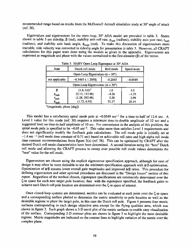
Eigenvalues and eigenvectors for the open-loop, 30 ° AOA model are provided in table 3. Statesshown in table 3 are sideslip, [3 (rad), stability axis roll rate, Pstab (rad/sec), stability axis yaw rate, rstab
(rad/sec), and stability axis bank angle, _stab (rad). To make this discussion of eigenvectors more
tractable, side velocity was converted to sideslip angle for presentation in table 3. However, all CRAFTcalculations for this paper were done using the models as given in the appendix. Eigenvectors areexpressed as magnitude and phase with the values normalized to the first element ([3) of the vector.
State
Table 3. HARV Open-Loop Eigenspace at 30° AOA
] Roll mode Spiral modeDutch roll mode
Open-Loop Eigenvalues (o_= 30 °)
not applicable --0.3465 ± 1.2058j -0.2045 -0.0549
Open-Loop Eigenvectors (t_ = 30°)
13 (1.0, 0.0) t 1.0 1.0Pstab (2.13, 112.96) -4.26 -1.35rstab (1.28,292.98) 2.58 2.99
.Ostab (1.72, 6.93) 21.17 26.14
t(magnitude, phase [deg])
This model has a satisfactory spiral mode pole at -0.0549 sec -I for a time-to-half of 12.6 sec. A
Level 1 value for this mode (ref. 30) requires a minimum time-to-double amplitude of 12 sec and a
suggested limit on time-to-half amplitude of 10 sec. For convenience in the analysis of this problem, the
spiral mode pole is specified to be -0.05 sec -1. This value more than satisfies Level 1 requirements and
does not significantly modify the feedback gain calculations. The roll mode pole is initially set at
-1.4 sec -1 (roll mode time constant of 0.71 sec) based on achievable roll rates and high-alpha roll mode
time constant recommendations from figure 3(a) (ref. 38). This can be optimized l_y CRAFT after the
desired Dutch roll mode characteristics have been determined. A second iteration using the "best" Dutch
roll mode and allowing the CRAFT process to sweep over possible roll mode values determines the"best" value for the roll mode.
Eigenvectors are chosen using the explicit eigenvector specification approach, although for ease of
design it may often be more desirable to use the minimum-specification approach with @/1_optimization.
Optimization of _/_ ensures lower overall gain magnitudes and improved t_/_ ratios. This procedure for
defining eigenvectors and other optional procedures are discussed in the "Design Issues" section of this
report. Regardless of the method chosen, eigenspace specifications are consistently determined over the
_-ta space for each new target pole location; then with the eigenspace specified, the feedback gains to
achieve each Dutch roll pole location are determined over the _-to space of interest.
Once closed-loop systems are determined, metrics can be evaluated at each point over the _-to spaceand a corresponding surface plotted to determine the metric sensitivity to pole location as well as the
desirable regions to place the target pole, in this case the Dutch roll pole. Figure 4 presents four metricsurfaces corresponding to each design objective area except for the flying qualities area, which was
shown in figure 3. Each graph shows a 3-D mesh plot of the metric surfaces to enable easy visualization
of the surface. Corresponding 2-D contour plots are shown in figure 5 to highlight the most desirable
regions. Metric magnitudes are indicated on the contour lines to highlight variation of the metric over thecomplex plane.
19
Control PowermDutch Roll Mode
The upper left-hand graphics of figures 4 and 5 present the control power metric from the first design
objective area; these graphs are labeled as "Mcp" as a function of frequency and damping ratio. For thisdesign example, Mcp was defined as a gain metric given by equation (25) and all feedback gains were
equally weighted in the calculations. Plotted in this fashion the metric is a sensitivity measure indicatingdesirable regions for the Dutch roll pole and preferred directions to move the pole if an adjustment is
desired. This surface gives an indication of where, in terms of pole placement, the greatest control power
demands will be placed on the control system. Low values of Mcp correspond to desirable values
(reduced gains), and high values in the high frequency region correspond to undesirable values (high
gains) and greater required control power. The lower damping ratios are favored in the sense of reducing
gain magnitudes; these values are closer to the open-loop value of the system.
For this eigenspace configuration and the target region considered, wide latitude exists for the choice
of damping with respect to control power. Relatively small gain metric values (Mcp < 2.0) fall in the
frequency range of 0.6 to 1.6 rad/sec for all damping ratios considered. High frequency requirements will
drive up control power required. The most desirable region naturally tends to be an area near the open-
loop pole where no feedback is required. If the open-loop eigenvectors had been chosen, zero gains
would be required for the point at (_, to) = (0.28, 1.25). For this example, however, the gain metric does
not go exactly to zero at the open-loop pole location because some feedback is still required to achieve
the desired eigenvector specification that does not correspond to the open-loop case.
Robustness--Dutch Roll Mode
For this example, robustness metrics for uncertainty at the inputs and outputs were determined based
on unstructured uncertainty models discussed in the "Robustness Metrics" section of this report. These
robustness measures are shown over a range of frequency and damping for the Dutch roll mode on the
bottom left- and right- hand sides of figures 4 and 5. The robustness metric is labeled "Mri" for
uncertainty at the input and "Mro" for uncertainty at the output.
Figure 5(c) shows that Mri, robustness to uncertainty at the inputs, begins to deteriorate with Dutch
roll frequencies above 1.6 rad/sec, but is well above the suggested datum of 0.5 for all values of
frequency and damping considered. For this example, Mri does not provide a hard design constraint;
consequently, the designer has flexibility in choosing the Dutch roll mode with respect to this metric. Onthe other hand, Mro, the robustness to uncertainty at the outputs, meets the 0.5 datum only in a region
between 1.2 and 1.45 rad/sec. Considering both robustness design metrics together, a fairly large
desirable region for Dutch roll frequency is obtained between 1.2 and 1.45 rad/sec.
Agility--Dutch Roll Mode
The graphic in the upper fight hand comer of figure 4 presents the airframe yaw agility metric, Mag.
Roll agility is not presented because there is little sensitivity of roll agility to Dutch roll mode placement
given the eigenspace chosen for this example. For the yaw agility metric, progressively greater valuesshow the more desirable values of agility, i.e., greater yaw acceleration. The 2-D contour plot, figure
5(b), has contour lines quantifying the value of the metric. As expected, the contour lines indicate that
increasing frequency and reducing damping will improve yaw agility. For maximum agility the most
desirable region is located at the lower fight-hand portion of the figure, where Mag ranges from0.4 rad/sec 2 to 0.5 rad/sec 2. Care must be used when comparing these metric values with measured or
simulated instantaneous values of yaw acceleration. This Mag is an average acceleration produced from a
20
q_| I-
stepinput. In addition,theinputis adjusted to provide the same ste_id);-_tate sideslip angle for each polelocation. Consequently, incorrect conclusions could result from a direct comparison with instantaneous
simulated or measured values. Design experience will indicate the best values for this metric; however,
sensitivity information is contained in the plot, and it provides an indicator of the best direction to move
the poles for increasing agility. In this example, the agility metric indicates that, to achieve the most yawagility, the designer should choose the highest frequency and lowest damping that still satisfies the othermetrics.
Flying Qualities--Dutch Roll Mode
The fourth design objective area covers pilot-in-the-loop requirements. A presentation of flying
qualities specifications for the roll and Dutch roll modes is given in figure 3. Included in this figure are
roll mode specifications for gross acquisition at 30 ° AOA. Because no high AOA design guidelines exist
for the Dutch roll mode, the requirement for low feedback gain magnitudes (i.e., Mcp) will be weighted
heavily. In addition, the low AOA flying qualities requirements for Dutch roll frequency and damping
will be satisfied only if no contradiction exists with the other metrics. Given this design viewpoint, the
Moorhouse-Moran suggested minimum Dutch roll frequency of 1.0 rad/sec will be readily satisfied.
For this example, the flying qualities metrics are known before the design closed-loop systems are
calculated. Although no flying qualities metrics need to be calculated for the closed-loop system, a
designer may choose to apply other criteria that may require computation. For example, criteria such as
Neal-Smith, Smith-Geddes, or Backdrop criteria (refs. 39-41) could be applied in a longitudinal problem.
Composite/Contour OverlaymFinal Design--Dutch Roll Mode
For this example problem, only five metrics are involved, and an astute designer may quickly
determine the best design compromise by just considering figures 3-5. However, in a general design
problem many more metrics may be involved, making the analysis more difficult. In the CRAFT design
approach, to make determination of the best design region for a target pole more tractable, a compositemetric surface is formed over the _-¢0 design space.
The CRAFT composite surface reflects all the metrics by increasing in value where desirable-metricregions overlap and where the net sum of metrics is increasing. The composite surface is formed by first
normalizing all metric surfaces shown in figure 4 to unity, i.e., the best (usually the largest) value is set to
one. Dutch roll flying qualities specification (labeled "Mdr" in figure 6), is represented as a flat surface
equal to one and is used to reflect the Level 1 region (_DR > 0.4, 0_R>I.0 ) of the flying qualities metric
defined in figure 3(b). The normalized metric surfaces are then summed together. If a metric has the
convention of increasing positive values indicating improvement, it can be summed directly. If a metricsuch as the control power metric, Mcp, is included, it must be modified to the same convention before
being added to the composite surface. Because Mcp has an improving value as the metric value becomes
smaller, it requires an "inversion" before being added to the composite. This is accomplished bysubtracting the normalized metric from one. The result is that the new metric now has larger values close
to one as the control power required becomes more favorable, i.e., as control power required is reduced.
For this example problem, figure 6(a) shows the composite metric surface. Since all 5 metrics are
represented in this figure, a maximum value close to 5 is possible but not likely, because that would
require the best points of each metric to occur at the same values of _ and co. One variation on this
process is to have weights multiply the normalized metrics to reflect individual designer requirements.No weights are used in this example.
21
The "best" design choice is a region where all metric desirable regions overlap with their greatest
values. In practice, it is not likely to have all the desirable regions overlap, so the best design choice is
where most metric desirable regions overlap. The best region is easily seen by considering a contour
representation of the composite surface, as shown in figure 6(b), "Composite metric contours." In this
graphic the best design region is centered on to = 1.3 and extends from 4 = 0.4 to 0.8, with the peak
occurring at (4, to) = (0.4, 1.3). A smaller or more definitive best design region could be determined by
using contours with more resolution; however, little is gained in the final analysis. Using designer's
discretion, composite metric values greater than 3.0 will be considered adequate and greater than 3.5 asmost desirable.
The designer's final decision can be simplified by observing some of the key desirable regions
superimposed over the composite metric contour graphic. The most desirable regions of all five metrics
in figures 3 and 5 are shown together in figure 6(c), "Metric desired regions." For this design example,
the desirable region for the control power metric, Mcp, was chosen to be Mcp < 1.0. This region
corresponds to the contour labeled as "1" in both figures 5(a) and 6(c). The desirable region for bothrobustness metrics was chosen as the region with magnitudes > 0.5. For Mro, this region is defined by
two vertical solid-line contours labeled as "0.5" in figures 5(d), 6(c), and 6(d). The other robustness
metric, Mri, was satisfactory over the entire region considered and therefore its contour is not shown in
figure 6. In this graphic, the most desirable regions of all the metrics overlap except for the agility metric,
Mag, which has its largest values (0.4-0.5 rad/sec 2) in the low damping and high frequency region.Unfortunately, very limited specifications exist for agility of advanced fighter aircraft, and no
specification exists for this specific metric. However, experience with HARV indicates that values of0.1 to 0.2 rad/sec 2 may be acceptable for this metric when considering HARV-like aircraft at 30°AOA.
The fifth metric used in this example is the flying qualities metric, shown as dashed lines in figure 6(c)
and labeled as Mdr, defining Level 1 to be where _-_OR> 0.4 and toDR > 1.0 for the Dutch roll damping and
frequency.
Figure 6(d), labeled as "Composite/contour overlay," has the composite contour regions shown as
shaded areas, the lighter shade indicating the more desirable region. Superimposed on the same graphic
are desirable regions for the control power metric, Mcp, the robustness metric, Mro, and the agility
metric, Mag. At this point the final design decision can easily be fine-tuned. Starting at the apparent
"best" design point [near (4, to) = (0.4, 1.3)], the designer may choose to make some important tradeoffs
to suit the particular design problem at hand. For example, 4 = 0.4 is at the edge of the desirable region
(because it is the edge of Level 1 flying qualities), and it may be more desirable to move the final design
point up to a higher damping ratio. As seen in this graphic, the designer has flexibility to move as far up
as 4 = 0.8 without substantially reducing the values of the other metrics. This region maintains Level 1
flying qualities, good robustness to model error at the input or output, and relatively low gains. Muchless freedom exists for changing the design Dutch roll frequency, however, if the designer is striving for
greater agility. In this case, the designer must trade off robustness for agility. For example, moving from
approximately (4, to) = (0.4, 1.2) to (4, to) = (0.4, 1.6) would double the agility metric from 0.i to0.2 rad/sec2, but it would move out of the acceptable robustness region. Since the robustness metric used
in this study is very conservative, this may be acceptable. Clearly, the final design requires judgment by
the control designer; even more judgment may be required at times, because the best region of an
individual metric does not always overlap the other metrics. This complication highlights the nature of
control design, which often requires tradeoffs in order to achieve a final overall design. An insightful
choice is more readily made using the CRAFT approach because the desirable regions and relative
tradeoffs of important metrics are graphically displayed. The designer's choice for a final design of the
Dutch roll pole might be chosen with a damping value between 0.4 and 0.6 and a frequency between 1.2and 1.45 rad/sec. However, the flying qualities specification for Dutch roll damping has not been
22
developedfor highAOAflight. Therefore,in thisexample,thedesignchoicewill beto giveupagilityformorestabilityandselectadampingandfrequencyof 0.7 and 1.25 rad/sec, respectively.
Composite OverlaymFinal Design--Roll Mode
Using the design selection above for Dutch roll mode, the corresponding roll mode overlay can be
developed by performing a CRAFT survey. Figure 7(a) shows the results of evaluating the same designmetrics for a roll mode variation. The survey is performed using the same eigenvector design process as
for the Dutch roll survey. For this case, the Dutch roll mode is held fixed to the design specified above
while the roll mode is allowed to vary from-4.2 sec -1 to -0.2 sec -1.
Figure 7(a) shows that increasing control power (Mcp) is required to drive the roll mode to faster
values. It reaches its lowest values close to the open-loop roll pole location, 0.2 sec-_. This figure also
shows the multivariable robustness metric at the output (Mro) as constant over the range of roll mode
considered and therefore it is not a constraint in this design problem. Multivariable robustness at the
input (Mri), on the other hand, shows improved or greater values as the roll mode frequency is reduced.
Thus, control power demands and robustness are improved as the roll mode is moved to slower values.
However, agility degrades with slower placement of the roll mode, as indicated by Mag. The vertical
boundary shown in figure 7(a) is a lower limit for the roll mode value as determined from figure 7(b).
This particular aircraft achieves maximum stability axis roll rates of 50 deg/sec when operating at 30°
AOA. The maximum roll rate is not determined by the inner loop dynamics and therefore must be input
to this design process. Various criteria have been used to determine the best roll rate to design into this
system, such as the roll overshoot criteria from reference 17. Given 50 deg/sec as a design constraint, the
McDonnell Aircraft flying qualities specification from figure 3(a), replotted on figure 7(b), indicates a
lower limit for roll mode placement of -0.8 sec -1. Since this aircraft model is not capable of satisfying
design criteria at higher roll rates, the designer is forced into the Level 2 region.
For this design example, the results of the roll mode overlay indicate that a final design choice, with
roll mode equal to -1.4 sec-I would be satisfactory. With this design choice, desirable levels of
robustness are provided, close to minimum gain magnitudes have been obtained (inferring reduced
control power required), and at least Level 2 flying qualities have been achieved. This design reflects a
choice to trade off maximum roll agility for reduced control power and robustness while respecting flyingqualities requirements.
In some cases, further analysis to assess the sensitivity of the roll mode placement on Dutch roll mode
overlay might be needed. In this case, however, a repeated CRAFT analysis is not necessary. First, the
final roll mode chosen is identical to that used in the Dutch roll mode survey, so there is no change in the
Dutch roll survey. Second, additional analysis would not be needed even with a fairly wide range of
choices for roll mode since the eigenvectors have been designed to decouple the lateral and directional
characteristics. The two surveys are somewhat insensitive to each other because of the decoupledeigenvectors.
The final feedback gains determined using CRAFT for this example provide excellent modal
characteristics and decoupling of roll and Dutch roll modes as desired. However, further design isrequired to obtain a system that gives satisfactory response to pilot inputs. Proper design of feedforward
command gains and crossfeeds are also required to obtain a complete, final design ready for pilotcommands. Feedforward design is beyond the scope of this paper, but the subject is addressed inreference 26.
23
Design Issues
Many issues arise for the designer in determining a feedback system for flight. A key concern for the
designer using the CRAFT approach with DEA is the determination of a desired eigenspace. This
concern is a result of very limited information in the literature on specifying eigenvectors. Fortunately,there is a substantial amount of literature for specifying eigenvalues, although this information is
predominantly limited to low AOA. The experience gained in this study designing suitable eigenvectorsis discussed in the next section.
One issue that has been removed from the example in this paper, but significantly affects the
eigenspace design, concerns redundant control effectors. By using Pseudo Controls in the design model,
two independent and orthogonal controls, providing directional and lateral control, replace theconventional redundant controls. The redundant yaw controls are mapped into one independent
directional control effector with minimal lateral coupling, and similarly, all the roll control effectors are
mapped into an independent lateral control with minimal directional coupling. More details of this
approach can be found in reference 25, and details of the application of Pseudo Controls and CRAFT tothe HARV control law are found in reference 26. With independent and orthogonal controls, design
complexity is greatly simplified, the designer has better insight into the design problem, and
implementation costs are significantly reduced. An additional benefit to the designer using DEA is a
clear picture of how many elements of the eigenvectors can be exactly specified.
Another issue for the designer, not addressed by this study, is determining the proper set of feedback
signals. Although this issue is problem dependent, the choice directly affects the ability of the control
system to meet performance specifications. In particular, the choice of feedback measurements and the
number of independent feedback measurements directly determine the achievable eigenspace for the
closed-loop system. With the DEA approach, each independent feedback measurement allows exact
placement of one system eigenvalue. The choice of feedbacks for the example in this paper reflects theconstraints of accurate and reliable sensors available for the control law in HARV.
The CRAFT design process provides a mechanism to sort many competing design issues and allow the
designer to find desirable placement for the system eigenvalues. However, one issue in the design
process involves proper selection of desirable eigenvector characteristics. These characteristics may beconstant or variable as the CRAFT survey is performed over the complex plane. Consequently, the
designer may require multiple eigenvalue surveys to assess metric sensitivity to design eigenvectors. To
demonstrate the sensitivity to eigenvector choice, Mcp is considered for each of the three basiceigenvector design approaches described previously, i.e., open-loop, minimum-specification, and desired-
model eigenvectors. Mcp defines RMS gain magnitude that reflects demands on the control system to
change system dynamics from existing open-loop characteristics to desired closed-loop characteristics.The more demanding changes in terms of eigenvalues or eigenvectors are reflected in the greater
magnitude of this metric.
System scaling is an issue that arises when using DEA and CRAFT, because it can help with
interpretation of the eigenvectors in the design process. System scaling, however, was not used in thisstudy because Psuedo Controls attempt to provide a unity transfer function to the feedbacks. Only scaling
for final presentation of eigenvectors is used in this report, as noted previously. From a control designer' s
point of view it is important to note that scaling the system, implemented as a similarity transform, affects
the eigenvectors and gains that result from the design process. Therefore, interpretation of gains andeigenvectors must be done with knowledge of any scaling. However, the system responses and
eigenvalues are independent of similarity transforms on the system.
24
To demonstrate the impact of eigenvector choice on design, the Current work performs analysis with
four different eigenvector specifications. For each case the control power metric, Mcp, is considered as a
function of Dutch roll mode frequency and damping. In all four cases, eigenvector design choices have
been applied to the 30 ° AOA model for calculating feedback gains and to the Mcp metric. The first two
cases considered utilize open-loop eigenvectors that remain constant as the Dutch roll mode pole is
varied. These two cases utilize open-loop eigenvectors that are taken from 5 ° and 30 ° AOA models,
respectively. The third and fourth cases utilize minimum-specification and desired-model eigenvectors.
For these eigenvector choices, the eigenvector specification varies with choice of Dutch roll mode pole.
Open-Loop Eigenvectors
The first approach for eigenvector design considered in this study was the use of the open-loop
eigenvectors of the system. As described earlier, this approach works well with an aircraft that behaves
classically already but may need some adjustments to its eigenvalues. The resulting eigenspace for the
30 ° AOA design point, using 5 ° AOA open-loop eigenvectors as desired eigenvectors, is shown in
table 4. Transformation of side velocity, v, to sideslip, [3, has not been done for these eigenspace
comparisons, so comparisons of desired and achieved eigenvectors, as well as the impact of eigenvector
choice on RMS gains (Mcp), can be made directly.
Table 4. Design Closed-Loop Eigenspace at 30 ° AOA
Using 5 ° AOA Open-Loop Eigenvectors
State Dutch roll mode Roll mode Spiral mode
Final Design: Closed-Loop Eigenvalues
-0.8750 + 0.8927j -1.40 -0.050
Final Design: Desired Closed-Loop Eigenvectors
v (1.0, O.O)f 1.0 1.0
Pstab (0.0087, 134.0) -0.1133 0.0027
rstab (0.0026, 277.69) 0.0064 0.0337
t_stab (0.0052, 36.87) 0.0809 0.6312
Final Design: Achieved Closed-Loop Eigenvectors
V
Pstab
rstab
_stab
(1.0, 0.0)
(0.0064, -188.12)
(0.0044, -40.15)
(0.0052, 36.87)
1.0 1.0
-0.1133 -0.0295
0.0122 0.0718
0.0811 0.6312
*(magnitude, phase [deg])
The final design eigenvalues are exactly as desired, since there are four independent measurements in
this design problem. However, with only two independent controls, only two elements of each
eigenvector could be specified. The final achieved eigenvectors match the desired eigenvectors for those
elements that were weighted. For example, the first and last elements of the Dutch roll eigenvectors, the
first and second elements of the roll mode eigenvector, and the first and last elements of the spiral mode
eigenvector were weighted. Consequently, for these elements the achieved values match desired values
exactly.
The resulting eigenspace at the final design point, using 30 ° AOA open-loop eigenvectors as desired
eigenvectors, is given in table 5. Again the desired and achieved values of the eigenspaee match where
weights were applied in the DEA algorithm to force the match. As in the previous case, the unweighted
25
elements of the eigenvectors are allowed to vary in order to match, in a least squares sense, an achievable
eigenspace to the desired eigenspace. Considering the achieved eigenvectors from the two designs using
open-loop eigenvectors, one cannot easily discern the impact on the final design. Using design metrics
such as Mcp can provide more insight, because the final design is sensitive to these measures, and these
measures are important to the designer.
The impact on Mcp of choosing an open-loop eigenvector specification is shown in figures 8(a) and
8(b). These eigenvector specifications are constant as Dutch roll mode frequency and damping are varied
during the CRAFT survey. Figure 8(a) shows the impact of choosing desired eigenvectors from a 5°
AOA, open-loop model and figure 8(b) shows the results of choosing from a 30 ° AOA, open-loop model.
Comparing these two cases, the more classical eigenvector from the lower AOA model produced the
lower values of RMS feedback gains overall, and it produced the largest region of low Mcp values, i.e.,
values of Mcp < 2. This makes the designer's work easier, giving more freedom of choice for the final
pole placement. Both cases show regions of lower metric values near Dutch roll mode frequencies of
1 rad/sec; however, the shapes of the low valued regions and nearby gradients are substantially different.
Figures 8(a) and 8(b) highlight the sensitivity of the final design to choice of desired eigenvectors.
Table 5. Design Closed-Loop Eigenspace at 30 ° AOA
Using 30 ° AOA Eigenvectors
State Dutch roll mode Roll mode Spiral mode
Final Design: Closed-Loop Eigenvalues
not applicable -0.8750 + 0.8927j -1.40 -0.050
Final Design: Desired Closed-Loop Eigenvectors
v
Pstab
rsmb
_bstab
(1.0, 0.0)1
(0.0075, 112.96)
(0.0046, 292.98)
(0.0061, 6.93)
1.0
-0.0151
0.0091
0.0751
1.0
--0.0048
0.0106
0.0927
Final Design: Achieved Closed-Loop Eigenvectors
v
Psmb
rs_b
_s_b
0.0, 0.0)(0.0075, -218.62)
(0.0048,-40.28)
(0.0061, 6.93)
1.0
--0.0151
0.0060
0.0109
1.0-0.0043
0.0106
0.0927
¢(magnitude, phase [deg])
In general, as a CRAFT survey moves the values of the target closed-loop poles toward the open-loop
poles, while using the system open-loop eigenvectors, the gains will go to zero. However, the design
using 30 ° AOA, open-loop eigenvectors [shown in figure 8(b)] did not produce a large area of reduced
Mcp, and the gains did not go to zero near the open-loop pole locations. In this case, the lower gains are
not achieved because the 30 ° AOA eigenvectors are used in combination with eigenvalues that are not all
selected close to their open-loop values. For this design example, the desired closed-loop roll mode is
substantially different from the system's open-loop value; consequently, the final design has an
eigenspace different from an open-loop eigenspace that would have produced reduced feedback gains.
Feedback gain magnitudes generally reflect the degree of difference between open-loop and desired
closed-loop eigenspace.
Eigenvector choice has a significant impact on feedback gains. Unfortunately, there is not much
guidance available for determining the best eigenvectors. The open-loop eigenvector may be a valid
26
I _1-
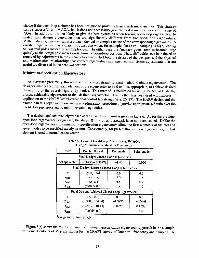
choice if the open-loop airframe has been designed to provide classical airframe dynamics. This strategycan be successful at low AOA, but it does not necessarily give the best dynamics over a full range ofAOA. In addition, it is not likely to give the best dynamics when forcing open-loop eigenvectors to
match with design eigenvalues that are significantly different from the open-loop eigenvalues.Mathematically, eigenvectors must match the real or complex nature of the corresponding eigenvalues. A
constant eigenvector may violate this constraint when, for example, Dutch roll damping is high, leadingto two real poles instead of a complex pair. In either case the feedback gains tend to become largequickly as the design pole moves away from the open-loop position. These difficulties can be reduced or
removed by adjustments in the eigenvectors that reflect both the desires of the designer and the physicaland mathematical relationships that connect eigenvalues and eigenvectors. Some adjustments that areuseful are discussed in the next two sections.
Minimum-Specification Eigenvectors
As discussed previously, this approach is the most straightforward method to obtain eigenvectors. The
designer simply specifies each element of the eigenvector to be 0 or 1, as appropriate, to achieve desired
decoupling of the aircraft rigid body modes. This method is facilitated by using DEA that finds theclosest achievable eigenvector to the "desired" eigenvector. This method has been used with success in
application to the HARV lateral-directional control law design (refs. 26, 27). The HARV design and the
example in this paper were done using an optimization procedure to provide appropriate _/13 ratio over theCRAFT design space and to minimize gain magnitudes.
The desired and achieved eigenspace at the final design point is given in table 6. As for the previous
open-loop eigenvector design case, the states, X = [v Pstab rstab_stab], have not been scaled. Unlike theopen-loop eigenvectors, the minimum-specification eigenvectors allow the first elements of the roll and
spiral modes to be specified exactly as zero. Consequently, for presentation of these eigenvectors, the lastelement is used to normalize the vector.
Table 6. Design Closed-Loop Eigenspace at 30° AOAUsing Minimum-Specification Eigenvector
State Dutch roll mode Roll mode Spiral mode
Final Design: Closed-Loop Eigenvalues
not applicable -0.8750 + 0.8927j -1.40 --0.050
Final Design: Desired Closed-Loop Eigenvectors
V
Pstab
rsmb
_stab
(1.0, 0.0)*(x.x, x.x)
(x.x, x.x)
(0.0065, 0.0)
0.01.0
X.X
X.X
Final Design: Achieved Closed-Loop Eigenvectors
0.0X,X
X.X
1.0
V
Pstab
rstab
t_stab
(1.o, o.o)(0.0080, 134.34)
(0.0049, -40.43)
(0.0065, o.o)
0.0-1.3975
0.0879
1.0
0.0
-0.0468
0.1138
1.0
*(magnitude, phase [deg])
Figure 8(c) shows the results of using the minimum-specification eigenvector approach in the example
problem. Contours of Mcp are shown for the CRAFT survey of Dutch roll frequency and damping. A
27
fairly largeareain thedesignspacebelowaDutchroll frequencyof 1.5rad/sechasverylow feedbackgains. A fairly sharpincreaseof Mcp occurswith this approachfor frequenciesbetween1.5and1.6rad/sec;above1.6rad/sec,themagnitudeof Mcplevelsoutto valuesslightlyunderthatfoundwiththe30° AOAopen-loopeigenvector.Thisrapidchangeingainsreflectsthesensitivityof feedbackgainsto eigenvectors.Partof this sensitivity is due to a limit on allowable t_/l_ ratios, which was reached during
the optimization to minimize RMS gain magnitude.
This sensitivity also reflects the need for caution when specifying eigenvectors in a minimum-
specification manner. Eigenvectors can be specified directly as linearly independent combinations ofzeroes and ones, as is often seen in the literature when eigenspace assignment is used. It provides a direct
way to decouple responses of aircraft states. However, this neither respects physical constraints of the
aircraft nor modal requirements that may exist. The choice of eigenvalue and eigenvector is closely
related to specifying the placement of poles and zeroes in a transfer function representation. Transferfunction zeroes are functions of aircraft physical characteristics; for example, T02 is directly tied to fLa.
Consequently, specifying nonaircraft-like values for these parameters may result in physically
unachievable eigenvectors and large gains. Fortunately, eigenspace assignment allows a solution for the
achievable eigenvectors that are as close to the desired eigenspace as possible, but there is no guarantee of
small gains at the solution point. Very high gains imply the theoretically achievable eigenspace is not
practical. The designer must work a tradeoff between desirable eigenspace and available control power.
Desired-Model Eigenvectors
Creating desired-model eigenvectors by first creating a state-space model that expresses the
eigenspace explicitly is an approach that has also been used with success. This method, although not assimple as the minimum-specification method, is straightforward. It does, however, require more a prioriinformation to create the desired state-space model. This additional information for the desired model
may not be available in some cases, for example, at high AOA conditions where there is limited design
experience.
Figure 8(d) shows the contours of Mcp for this choice of eigenvector design. This method produced
the lowest values of Mcp of all the approaches considered, reinforcing the idea that the RMS gains are
kept lowest with eigenvector designs that vary during the CRAFT survey. For the example, in the 30 °
AOA system in this paper, the desired-model approach provided a larger region of acceptable values for
Mcp than the minimum-specification approach. This result highlights the sensitivity of eigenvectorchoice because the resultant eigenvectors at the final design point are very similar between the two
methods. Table 7 shows the final design eigenspace resulting from design with desired-model
eigenvectors. The achieved eigenspace using desired-model eigenvectors appears very close to thatachieved using minimum-specification eigenvectors; however, it is clear from figure 8 that potentially
large differences exist from a control designer's point of view. These differences highlight the sensitivityof the control designer's problem to eigenspace choice and the need for a CRAbT design methodology.
28
'1 I1
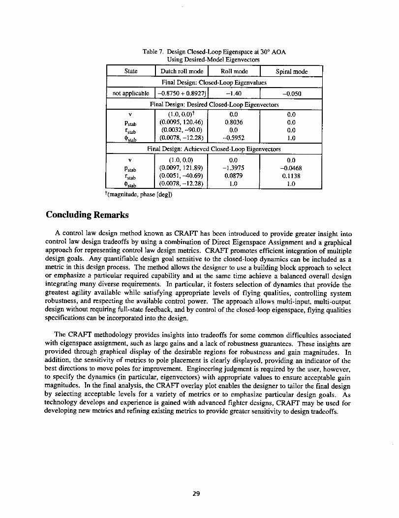
Table 7. Design Closed-Loop Eigenspace at 30 ° AOAUsing Desired-Model Eigenvectors
State Dutch roll mode Roll mode Spiral mode
Final Design: Closed-Loop Eigenvalues
not applicable -0.8750 + 0.8927j -1.40 -0.050
Final Design: Desired Closed-Loop Eigenvectors
v (1.0, 0.0)_ 0.0 0.0
Pstab (0.0095, 120.46) 0.8036 0.0rstab (0.0032, --90.0) 0.0 0.0_stab (0.0078, --12.28) -0.5952 1.0
Final Design: Achieved Closed-Loop Eigenvectors
v (1.0, 0.0) 0.0 0.0
Pstab (0.0097, 121.89) -1.3975 -0.0468rstab (0.0051, --40.69) 0.0879 0.1138_stab (0.0078, - 12.28) 1.0 1.0
t(magnitude, phase [deg])
Concluding Remarks
A control law design method known as CRAFT has been introduced to provide greater insight into
control law design tradeoffs by using a combination of Direct Eigenspace Assignment and a graphical
approach for representing control law design metrics. CRAFT promotes efficient integration of multipledesign goals. Any quantifiable design goal sensitive to the closed-loop dynamics can be included as a
metric in this design process. The method allows the designer to use a building block approach to select
or emphasize a particular required capability and at the same time achieve a balanced overall design
integrating many diverse requirements. In particular, it fosters selection of dynamics that provide the
greatest agility available while satisfying appropriate levels of flying qualities, controlling system
robustness, and respecting the available control power. The approach allows multi-input, multi-output
design without requiring full-state feedback, and by control of the closed-loop eigenspace, flying qualitiesspecifications can be incorporated into the design.
The CRAFT methodology provides insights into tradeoffs for some common difficulties associated
with eigenspace assignment, such as large gains and a lack of robustness guarantees. These insights are
provided through graphical display of the desirable regions for robustness and gain magnitudes. In
addition, the sensitivity of metrics to pole placement is clearly displayed, providing an indicator of the
best directions to move poles for improvement. Engineering judgment is required by the user, however,
to specify the dynamics (in particular, eigenvectors) with appropriate values to ensure acceptable gain
magnitudes. In the final analysis, the CRAFT overlay plot enables the designer to tailor the final design
by selecting acceptable levels for a variety of metrics or to emphasize particular design goals. As
technology develops and experience is gained with advanced fighter designs, CRAFT may be used for
developing new metrics and refining existing metrics to provide greater sensitivity to design tradeoffs.
29
References
1. Herbst, W. B.; and Krogull, B.: Design for Air Combat. AIAA 72-749, Aug. 1972.
2. Eidetics International, Inc: Tactical Evaluation of the Air-to-Air Combat Effectiveness of Supermaneuverability.
WRDC-TR-90-3035, June 1990.
3. McDonnell Aircraft Co., McDonnell Douglas Corp: Multi-System Integrated Control (MUSIC) Program.WRDC-TR-90-6001, June 1990.
4. Herbst, W.: Future Fighter Technologies. J. A irc., vol. 17, no. 8, Aug. 1980.
5. Hamilton, W. L.; and Skow, A.M.: Operational Utility Survey: Supermaneuverability. AFWAL-TR-85-3020,
Sept. 1984.
.
.
.
.
10.
11.
12.
13.
14.
15.
16.
Ogburn, M. E.; Nguyen, L. T.; Wunschel, A. J.; Brown, P. W.; Carzoo, S. W.: Simulation Study of Flight
Dynamics of a Fighter Configuration With Thrust-Vectoring Controls at Low Speeds and High Angles ofAttack. NASA TP-2750, 1988.
Foltyn, Robert W.; Skow, Andrew W.; Lynch, Urban H.; Lynch, Anerew M. P.; Laboy, Orlando J.; Arand,
Anthony J.: Development of Innovative Air Combat Measures of Merit for Supermaneuverable Fighters.AFWAL-TR-87-3073, Eidetics, Oct. 1987.
Hodgkinson, J., Skow, A.; Ettinger, R.; Lynch, U.; Laboy, O.; Chody, J.; Cord, T. J.: Relationships Between
Flying Qualities, Transient Agility, and Operational Effectiveness of Fighter Aircraft. AIAA 88-4327, Aug.1988.
Phillips, William H.: Analysis of Effects of lnterceptor Roll Performance and Maneuverability on Success of
Collision-Course Attacks. NACA RM L58E27, 1958.
McAtee, Thomas P.: Agility in Demand. Aerosp. America, May 1988.
Tamrat, B. F.: Fighter Aircraft Agility Assessment Concepts and Their Implication on Future Agile Fighter
Design. AIAA 88-4400, Sept. 1988.
Skow, Andrew M.; Hamilton, William L.; Taylor, John H.: Advanced Fighter Agility Metrics. AIAA 85-1779,
Aug. 1985.
Taylor, John H.; Skow, Andrew M.; Parker, Robert W.; Malcolm, Gerald N.; Folytn, Robert W.: Flight TestValidation of Advanced Agility Metrics for T-38 and F-4. USAF Contract F33615-85-C-0120, TR 86-212, Sept.1986.
Skow, Andrew M.; Foltyn, Robert W.; Taylor, John H.; Parker, Robert W.: Transient Performance and
Maneuverability Measures of Merit for Fighter/Attack Aircraft. USAF Contract F33615-85-C-0120, TR 86-201,Jan. 1986.
Murphy, P. C.; Bailey, M. L.; and Ostroff, A. J: Candidate Control Design Metrics for an Agile Fighter. NASA
TM-4238, 1991.
Foster, J. V.; Bundick, W. T.; and Pahle, J. W.: Controls for Agility Research in the NASA High-Alpha
Technology Program. SAE TP-912148, Sept. 1991.
17. Hoffler, K. D.; Brown, P. W.; Phillips, M. R.; Rivers, R. A.; Davidson, J. B.; Lallman, F. J.; Murphy, P. C.; and
3O
Ostroff,A.J.: EvaluationManeuverandGuidelineDevelopmentforHigh-AlphaControlLawDesignUsingPilotedSimulation.AIAA94-3512,Aug.1994.
18.Wilson,D. J.; and Riley, D. R.: Volume 1 and 2: Flying Qualities Criteria Development Through MannedSimulation for 60°Angle-of-Attack. NASA CR-4535, 1993.
19. Chambers, Joseph R.; Gilbert, William P.; Nguyen, Luat T., eds.: High-Angle-of-Attack Technology. NASACP-3149, 1990.
20. Matheny, N. W., compiler: High-Angle-of-Attack Projects and Technology Conference. NASA CP-3137, 1992.
21. Fourth High Alpha Conference. NASA CP-10143, 1994.
22. Fifth High Alpha Conference. NASA/CP-1998-207676, 1998.
23. Nguyen, Luat T.: Flight Dynamics Research for Highly Agile Aircraft. SAE TP-892235, Sept. 1989.
24. Murphy, P. C.; and Davidson, J. B.: Control Design for Future Agile Fighters. AIAA 91-2882, Aug. 1991.
25. Lallman, F. J.; Davidson, J. B.; and Murphy, P. C.: A Method for Integrating Thrust-Vectoring and Actuated
Forebody Strakes With Conventional Aerodynamic Controls on a High-Performance Fighter Airplane.NASA/TP-1998-208464, 1998.
26. Davidson, J. B.; Murphy, P. C.; Lallman, F. J.; Hoffler, K. D.; and Bacon, B. J.: High-Alpha Research Vehicle
Lateral-Directional Control Law Description, Analyses, and Simulation Results. NASA/TP-1998-208465,1998.
27. HARV Control Law Design Team: Design Specification for a Thrust-Vectoring, Actuated-Nose-Strake FlightControl Law for the High-Alpha Research Vehicle. NASA TM-110217, 1996.
28. Davidson, J. B.; and Schmidt, D. K.: Flight Control Synthesis for Flexible Aircraft Using EigenspaceAssignment. NASA CR-178164, 1986.
29. Srinathkumar, S.: Modal Control Theory and Application to Aircraft Lateral Handling Qualities Design.NASA TP-1234, 1978.
30. Military Standard--Flying Qualities of Piloted Aircraft. MIL-STD-1797A, Jan. 1990.
31. Shapiro, E. Y.; and Chung, J. C.: Flight Control System Synthesis Using Eigenstructure Assignment. J. Optim.Theory & Appl., vol. 43, no. 3, July 1984.
32. Farineau, J.: Lateral Electric Flight Control Laws of a Civil Aircraft Based Upon Eigenstructure AssignmentTechnique. AIAA 89-3594, Aug. 1989.
33. Unbehauen, H.; and Rao, G. P.: Identification of Continuous Systems, North-Holland Systems and ControlSeries. Elsevier Sci. Publ. Co., Inc., 1987.
34. Mukhopadhyay, V.; and Newsom, J. R.: A Multiloop System Stability Margin Study Using Matrix SingularValues. J. Guid., Navigat., & Control, vol. 8, no. 4, Sept.-Oct. 1984.
35. Bitten, R.: Qualitative and Quantitative Comparison of Government and Industry Agility Metrics. AIAA-89-3389-CP, Aug. 1989.
31
36.
37.
38.
39.
40.
41.
Moorhouse,D.J.;andMoran,W.A.:FlyingQualitiesDesignCriteriaforHighlyAugmentedSystems.IEEE
National Aerospace and Electronics Conference, NAECON, May 1985.
Riley, David R.; and Drajeske, Mark H.: Relationships Between Agility Metrics and Fl_ng Qualities. SAE
Aerospace Atlantic Conference, SAE TP-901003, April 1990.
Krekeler, Gregory C.; Wilson, David J.; and Riley, David R.: High Angle-of-Attack Flying Qualities Criteria.
AIAA 90-0219, .tan. 1990.
Neal, P. T.; and Smith, R. E.: An In-Flight Investigation to Develop Control System Design Criteria for Fighter
Airplanes. AFFDL-TR-70-74, vol. 1, Dec. 1970.
Smith, R.; and Geddes, N. D.: Handling Quality Requirements for Advanced Aircraft Design: Longitudinal
Mode. AFFDL-TR-78-154, Aug. 1979.
Gibson, J. C.: Piloted Handling Qualities Design Criteria for High Order Flight Control Systems. AGARD-
CP-333, 1982.
32
_1 1I _
Appendix
Open-loop system quadruples, describing 4th order, linear, lateral-dlrectional dynamics of HARV with
thrust-vectoring at 5 ° and 30 ° AOA, are shown below. System quadruples have the form of
which define state-space equations for states, X, controls, U, and measurements, Z, as
X=AX+BU
Z=MX+NU
System states are side velocity (ft/sec), stability-axis roll rate (rad/sec), stability-axis yaw rate (rad/sec),
and stability-axis bank angle (rad). Two Pseudo Control inputs are normalized pseudo lateral control and
normalized pseudo yaw control. Measurements for feedback are stability-axis roll rate, stability-axis yaw
rate, lateral acceleration at the sensor (g's), and sideslip rate (rad/sec). Trim values for total velocities are
598.0 ft/sec at 5 ° AOA and 282.0 ft/sec at 30 ° AOA.
Sys_05 =
Sys_30 =
-0.1305 0.1512 -597.5821 32.1667-0.0187 -1.5271 0.6757 0.0
0.0050 0.1152 -0.1529 0.00.0 1.0 0.0 0.0
0.0 1.0 0.0 0.00.0 0.0 1.0 0.0
-0.0021 0.0535 -0.0462 0.0-0.0002 0.0003 -0._92 0.0538
-0.0403 -0.1337 -282.2581 32.1549-0.0099 -0.3858 0.7811 0.0
0.0060 0.2001 -0.5262 0.00.0 1.0 -0.0280 0.0
0.0 1.0 0.0 0.00.0 0.0 1.0 0.0
-0.0007 0.0041 -0.0675 0.0--0.0001 -0.0005 -1.0009 0.1140
-2.0005 - 19.10221.1179 -0.19410.0096 1.35270.0 0.0
0.0 0.00.0 0.0
-0.0614 -0.0669-0.0033 -0.0319
-4.5212 -8.6376
0.6768 -0.21300.1948 1.19100.0 0.0
0.0 0.00.0 0.0
-0.0145 0.0296-0.0160 -0.0306
33
co
Model [
Control design ___
algorithm:direct eigenspace
assignmentFeedback Igains
Closed-loopanalysis system [_
Control design metric S codesirable regions --t"
Final control law
Best desi.gn
compromise
Figure 1. CRAFT control synthesis methodology.
lDesired eigenvector, Wai _N
Subspace spanned by \/
c°lumns °f [_iIn - A]- 1Bc"--',% /
Achievable eigenvector, Vai---/ "
Figure 2. Achievable eigenvector obtained through DEA.
34
I _|1
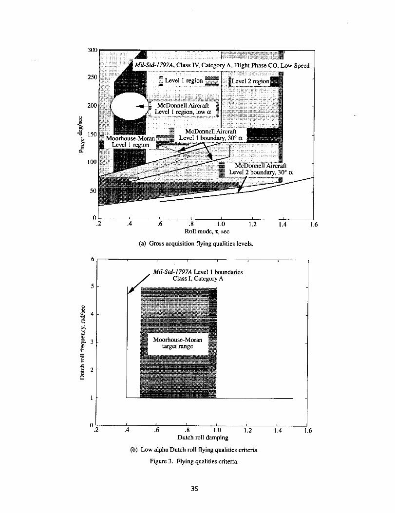
300 __ ,,m ................... K_:_iii!ili;_;_i,:i!i_i_i!iiiiii',iiii!i:!ili;ii_:!i!!!W'Mil-Std-1797A, Class IV, Category A, Flight Phase CO, Low Speed
250 _ Level 1 re_i 2_
200
150
100
50
Level 1 region
I I I
.6 .8 1.0 1.2
Roll mode, x, sec
(a) Gross acquisition flying qualities levels.
i i i I i i
!
1.4
3
0.2I
.4
Mil-Std-1797A Level 1 boundaries
Class I, Category A
i I I I
.6 .8 1.0 1.2
Dutch roll damping
(b) Low alpha Dutch roll flying qualities criteria.
Figure 3. Flying qualities criteria.
1.4 1.6
35
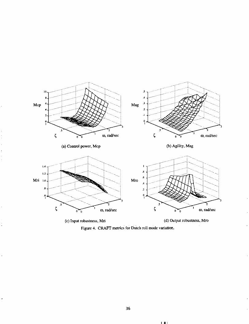
Mop
Mri
I0,
8,
6,
4.
2.
O.I
1,4.
1.2.
1.0.
,8
.6l
..-¢.
o o co, rad/sec
Mag
....-- , ".
.- -" "i "° """"""" ";" "" ... "'"r..
• ..'" ""'. ""- 3
co, rad/sec
(a) Control power, Mcp (b) Agility, Mag
°.°.- ,o
......... :'::'-.. "''"-._ " 3
Mro
........._......i/.i..........i....iiii.....:....
3
• °.
o o co, rad/sec
(c) Input robustness, Mri (d) Output robustness, Mro
Figure 4. CRAFT metrics for Dutch roll mode variation.
36
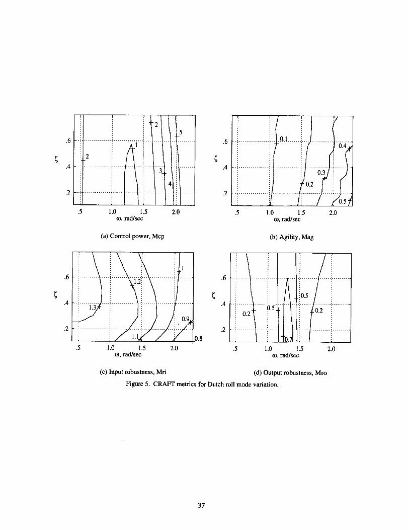
.6
.4
.2
.6
.4
.2
• 2 1,.
IL.!.
.5 1.0 1.5to, rad/sec
21 " "
i -4-
...... 4--I ........
3!itiit..
i
2.0
.6
.4
.2
t'Ii::...............i..............!.......0:3!.......
.5 1.0 1.5 2.0to, rad/sec
(a) Control power, Mcp (b) Agility, Mag
.5 1.0 1.5 2.0to, rad/sec
1
0.9_
0.8
.6
.4
.2
!.......!.5 1.0
li......"''4""
0.71
1.5
0.5
0.2
.....t ......... i .........!
2.0to, rad/sec
(c) Input robustness, Mri (d) Output robustness, Mro
Figure 5. CRAFT metrics for Dutch roll mode variation.
37
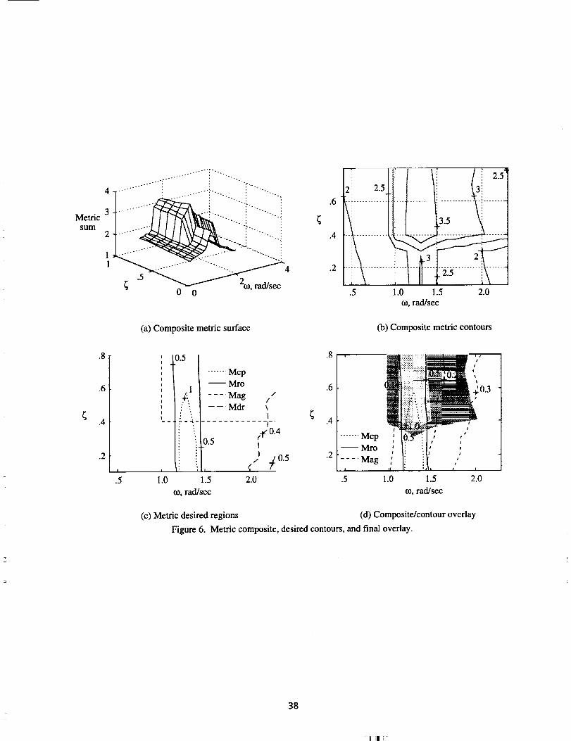
Metricsum
.8
.6
.4
.2
4
3
2
1
5 ........... "........... "....... i4
(a) Composite metric surface
i i i i 25_21 2.51 i 3!
.5 1.0 1.5 2.0co, rad/sec
(b) Composite metric contours
!
.5
0.5
i o.5
i i: •
1.0 1.5
0_, rad/sec
....... McpMro
.... Mag / /- --Mdr \
I
.8 ,
.6
.4
r-le"0.4I
/I 7_0.5 .2¢2.0
!_!_!ii........................,,-7--
0.3
....... I t+.-
I ! !
Mlro ! I I
Mag ,| | I I
.5 1.0 1.5 2.0
co, rad/sec
(c) Metric desired regions (d) Composite/contour overlay
Figure 6. Metric composite, desired contours, and final overlay.
38
'!-_ 1-
O
@
Z_
O
t_
2.5
2.0
1.5
1.0
0.5
0-4._
150
100
50
Mcp_ _ __,,,,%,
I I I I I I I
-4.0 -3.5 -3.0 -2.5 -2.0 -1.5 -1.1Roll mode, 1/sec
(a) CRAFT overlay for roll mode survey
Level 2/3
boundary
\
I
-.5 0
r 1 i
Design Pmax = 50 deg/sec
0 ___...1. L 1 1 L ..1__-4.5 -4.0 -3.5 -3.0 -2.5 -2.0 -1.5 -1.0 -.5
Roll mode, l/sec
1 T--T--T_ F
Level 1/2 boundary _
/
-_v_lLevel 2/3 boundary
(b) CRAFT overlay for roll mode survey
Figure 7. Roll mode requirements for gross acquisition.
39
1
: i
,6 "'i .....
.4: ......
.2_--_......
.5
.6
.4
.2
I
i 3 5
3 2 i
1.0 1.5 2.0
co, rad/sec
I I
!!!! !!!!.4
.2
.5 1.0 1.5 2.0tO, rad/sec
(a) Constant open-loop eigenvector 5° AOA (b) Constant open-loop eigenvector 30° AOA
| ;
i , ,
........ i.................i
.5
l........ii
1.0 1.5 2.0
(O, l'ad]sec
.6i--i...............!.............................3--.i i 2
,2 _ ...............................
[ ti
.5 1.0 .5 2.0
(0, rad/sec
(c)Minimum-specification eigenvector (d) Desired-model eigenvector
Figure 8. Variation of control power metric, Mcp, with eigenvector selection.
40
:1 11
Form ApprovedREPORT DOCUMENTATION PAGE oMBNo.077_-0188
Public reporting burden for this collection of Information is estimated to average 1 hour per response, Including the time for reviewing instr_ns, searching e0<isttngdata sources,getherlng and maintaining the data needed, and completing and reviewing the collection of information. Send comments rege_dtng this burden estimate or any other espect of thiscolleclfon of information, Including suggestions for reducing this burden, to Washington Headquarters Services, Directorate for Information Operations and Reports, 1215 JeffersonDavis Highway, Suite 1204, Arlington, VA 22202-4302, and to the Office of Managernerd and Budget, Papenvork Reduction Project (0704-0188), Washington, DC 20503.
1
1. AGENCY USE ONLY (Leave blank) 2. REPORT DATE 3. REPORT TYPE AND DATES COVERED
September 1998 Technical Publication4. TITLE AND SUBTITLE 5. FUNDING NUMBERS
A Control Law Design Method Facilitating Control Power, Robustness,Agility, and Elying Qualities Tradeoffs: CRAFT WU 505-68-30-05
]6. AUTHOR(S)
Patrick C. Murphy and John B. Davidson
7. PERFORMING ORGANIZATION NAME(S) AND ADDRESS(ES)
NASA Langley Research CenterHampton, VA 23681-2199
9. SPONSORING/MONITORINGAGENCYNAME(S)ANDADDRESS(ES)
National Aeronautics and Space AdministrationWashington, DC 20546-0001
8. PERFORMING ORGANIZATION
REPORT NUMBER
L-17571
10. SPONSORING/MONITORING
AGENCY REPORT NUMBER
NASA/TP-1998-208463
11. SUPPLEMENTARY NOTES
12a. DISTRIBUTION/AVAILABILITYSTATEMENT
Unclassified-Unlimited
Subject Category 08 Distribution: StandardAvailability: NASA CASI (301) 621-0390
12b. DISTRIBUTION CODE
13. ABSTRACT (Maximum 200 words)
A multi-input, multi-output control law design methodology, named "CRAFT', is presented. CRAFT stands forthe design objectives addressed, namely, Control power, Robustness, Agility, and Elying Qualities Tradeoffs. Themethodology makes use of control law design metrics from each of the four design objective areas. It combineseigenspace assignment, which allows for direct specification of eigenvalues and eigenvectors, with a graphicalapproach for representing the metrics that captures numerous design goals in one composite illustration. Sensitiv-ity of the metrics to eigenspace choice is clearly displayed, enabling the designer to assess the cost of designtradeoffs. This approach enhances the designer's ability to make informed design tradeoffs and to reach effectivefinal designs. An example of the CRAFT methodology applied to an advanced experimental fighter and discussion:of associated design issues are provided.
14. SUBJECT TERMS
Control law design; Design tradeoffs; Feedback control; Feedback gains; Output feed-back; Eigenspace assignment; High performance aircraft; High angle of attack; Fighteraircraft; Metrics; Agility; Robustness; Flying qualities; Handling qualities
17. SECURITY CLASSIFICATION 18. SECURITY CLASSIFICATION 19. SECURITY CLASSIFICATION
OF REPORT OF THIS PAGE OF ABSTRACT
Unclassified Unclassified Unclassified
NSN 7540-01-280-5500
15. NUMBER OF PAGES
45'16. PRICE CODE
A03
20. LIMITATION
OF ABSTRACT
Standard Form 298 (Rev. 2-89)
Prescdbed by ANSI Std. 239-18298-102
42

41