A Contribution to the Validation of the Electromagnetism Module in

12th

International LS-DYNA® Users Conference Electromagnetic(2)

1

Simulation of a Railgun: A contribution to the validation of

the Electromagnetism module in LS-DYNA® v980

Iñaki Çaldichoury

Pierre L'Eplattenier

Livermore Software Technology Corporation

7374 Las Positas Road

Livermore, CA 94551

Abstract A railgun is an electrical gun using electromagnetic forces in order to accelerate and launch projectiles

at several times the speed of sound. Railguns have long belonged to the science-fiction world or existed

as experimental and demonstrator technology. However in recent years, the U.S Navy has shown an

increased interest for Railguns as they offer the potential for reduced logistics and firing power. The

purpose of this paper is to simulate a railgun model using the Electromagnetism solver in LS-DYNA, to

compare results with existing analytical models and to show how LS-DYNA may help to improve such

existing models.

1- Introduction

An electromagnetism (EM) module is under development in LS-DYNA in order to

perform coupled mechanical/thermal/electromagnetic simulations [1], [2], [3]. This module

allows us to introduce some source electrical currents into solid conductors, and to compute the

associated magnetic field, electric field, as well as induced currents solved in the Eddy current

approximation.

One of the solver’s recent developments is the electromagnetic contact feature that allows

two conductive parts to come into contact and to exchange current with one another. The purpose

of this paper is to simulate a railgun model using the Electromagnetism solver in LS-DYNA in

order to validate this new feature. The railgun is an electrical gun using electromagnetic forces in

order to accelerate and launch projectiles at several times the speed of sound. Railguns have long

belonged to the science-fiction world or existed as experimental and demonstrator technology.

However in recent years, the U.S Navy has shown an increased interest for Railguns as they offer

the potential for reduced logistics and firing power. Results will be compared to an analytical

model and comments will be made on how LS-DYNA may be used to improve such existing

simple models. Finally, other applications of the LS-DYNA electromagnetic contact feature will

be mentioned.

Electromagnetic(2) 12th

International LS-DYNA® Users Conference

2

2- Railgun analytical system description

In its most basic form, a railgun consists of two parallel metal rails connected to an

electric power supply. When a projectile is inserted between the two bars, it provides a

conductive path between the rails thus completing the circuit. The current flowing through the

rails and armature generates a magnetic field between the bars which, in turn, creates a Lorenz

force applied on the projectile (See Figure 1).This force will propel the projectile and then eject

it from the end of the railgun at a very high speed. Based on the physical equations for this

problem and on some hypotheses that will be further discussed, this section describes a simple

analytical model that can be used to simulate a railgun model as proposed by [4] :

Figure 1 Schematic representation of a Railgun model

The chosen system consists in a storage capacitor ( circuit) connected to the railgun bars

and discharging when the railgun is ready to fire. The circuit equation gives:

𝑞

+𝑑( 𝑖)

𝑑𝑡+ 𝑖 = 0

where 𝑞 is the circuit charge, the circuit capacity, the whole circuit's inductance (rails,

projectile and power source), 𝑖 the current and the whole circuit's resistance .

The current can be expressed as a function of the charge:

𝑖 =𝑑𝑞

𝑑𝑡

The initial conditions yield:

𝑞(0) = 𝑑𝑞(0)

𝑑𝑡= 0

where is the initial charge of the capacitor ( = with being the initial voltage

applied to the system).

We now get:

𝑞

+𝑑

𝑑𝑡 𝑑𝑞

𝑑𝑡+

𝑑 𝑞

𝑑𝑡 +

𝑑𝑞

𝑑𝑡= 0

12th


3

With: 𝑑

𝑑𝑡=𝑑

𝑑

𝑑

𝑑𝑡=

𝑑

𝑑

where is the projectile’s velocity and

is now only dependent of the geometry.

Furthermore, the Lorentz force applied to the projectile can be written as [5]:

= 𝑑

𝑑𝑡=

𝑖 𝑑

𝑑

with M being the mass of the solid.

In order to solve these equations, a representation of the resistance's and inductance's behavior as

a function of the projectile's displacement x are needed. The circuit's resistance can be computed

as:

= + + = +

+

where is the initial resistance of the power source ( circuit), , the material's

conductivity, the size of the projectile (See Figure 2) and the surface through which

the current flows.

The behavior of the inductance of the rail gun system is not known. A first approach would be to

use the expression of the external inductance for parallel plane transmission lines. According to

this model, the inductance of the rail gun reads:

= +

where would be the initial inductance of the power source ( circuit), the

permeability of free space and , the railgun’s width (See Figure 2).

Figure 2 Geometry of the Railgun model



4

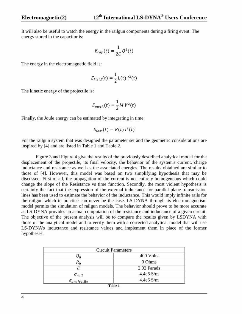
It will also be useful to watch the energy in the railgun components during a firing event. The

energy stored in the capacitor is:

(𝑡) =

(𝑡)

The energy in the electromagnetic field is:

(𝑡) =

(𝑡) 𝑖 (𝑡)

The kinetic energy of the projectile is:

(𝑡) =

(𝑡)

Finally, the Joule energy can be estimated by integrating in time:

(𝑡) = (𝑡) 𝑖 (𝑡)

For the railgun system that was designed the parameter set and the geometric considerations are

inspired by [4] and are listed in Table 1 and Table 2.

Figure 3 and Figure 4 give the results of the previously described analytical model for the

displacement of the projectile, its final velocity, the behavior of the system's current, charge

inductance and resistance as well as the associated energies. The results obtained are similar to

those of [4]. However, this model was based on two simplifying hypothesis that may be

discussed. First of all, the propagation of the current is not entirely homogeneous which could

change the slope of the Resistance vs time function. Secondly, the most violent hypothesis is

certainly the fact that the expression of the external inductance for parallel plane transmission

lines has been used to estimate the behavior of the inductance. This would imply infinite rails for

the railgun which in practice can never be the case. LS-DYNA through its electromagnetism

model permits the simulation of railgun models. The behavior should prove to be more accurate

as LS-DYNA provides an actual computation of the resistance and inductance of a given circuit.

The objective of the present analysis will be to compare the results given by LSDYNA with

those of the analytical model and to verify them with a corrected analytical model that will use

LS-DYNA's inductance and resistance values and implement them in place of the former

hypotheses.

Circuit Parameters

400 Volts

0 Ohms

2.02 Farads

4.4e6 S/m

4.4e6 S/m Table 1

12th


5

Railgun Geometry Parameters

1 m

30 mm

𝑖 30 mm

𝑖 10 mm

𝑡𝑖 20 mm Table 2

Figure 3 Railgun variables during firing given by the analytical model



6

Figure 4 Railgun Energy variables during firing given by the analytical model

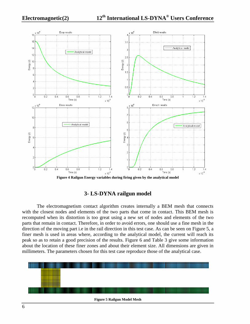
3- LS-DYNA railgun model

The electromagnetism contact algorithm creates internally a BEM mesh that connects

with the closest nodes and elements of the two parts that come in contact. This BEM mesh is

recomputed when its distortion is too great using a new set of nodes and elements of the two

parts that remain in contact. Therefore, in order to avoid errors, one should use a fine mesh in the

direction of the moving part i.e in the rail direction in this test case. As can be seen on Figure 5, a

finer mesh is used in areas where, according to the analytical model, the current will reach its

peak so as to retain a good precision of the results. Figure 6 and Table 3 give some information

about the location of these finer zones and about their element size. All dimensions are given in

millimeters. The parameters chosen for this test case reproduce those of the analytical case.

Figure 5 Railgun Model Mesh

12th


7

Figure 6 Railgun meshing zones

Railgun Mesh information

𝑡 𝑖 (x-direction) 2 mm

𝑡 𝑖 (x-direction) 0.5 mm




𝑡 𝑖 (x-direction) 9.5 mm

𝑡 𝑖 𝑡𝑖 1.875 mm

Total number of nodes 100 000

Total number of elements 80 000 Table 3

4- Results

The magnetic field generated by the circuit behind the projectile can be seen on Figure 7.

Figure 8 offers a view of the current density at two different times, when the projectile reaches

the very fine mesh defined as zone 2 and when it reaches the coarse mesh defined as zone 6.

When the projectile crosses zone 2, a very small gap where the current density is null (blue

color) between the projectile base and the rail can be observed. This is due to the BEM mesh that

"occults" the closest elements of the rail in contact with the projectile. When the projectile

crosses the coarser mesh of zone 6, this gap where no current diffusion is calculated, logically

grows. However, by the time the projectile reaches this zone, the railgun is almost entirely

discharged and it is believed that the influence on the results of this coarser mesh can be

neglected.

Figure 7 Magnetic field during firing



8

Figure 8 Current density when a) projectile is crossing zone 2 and when b) projectile is crossing zone 6

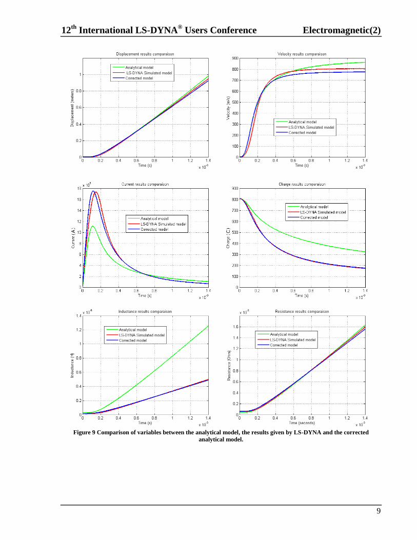
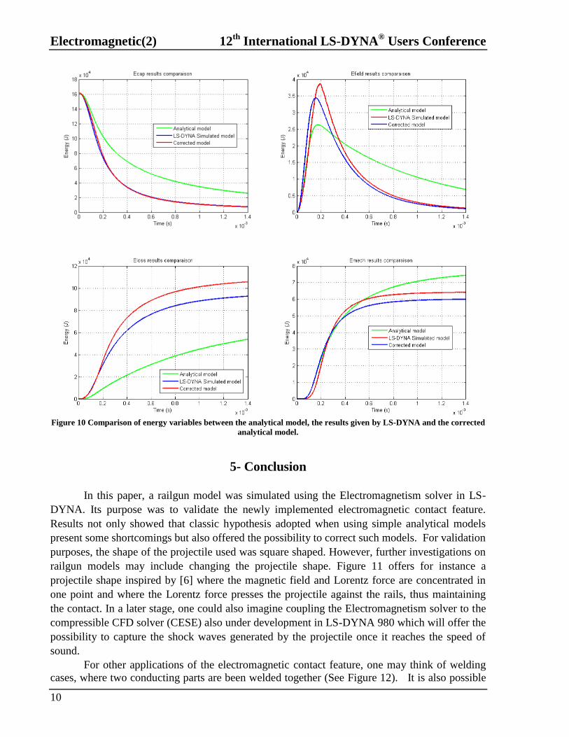
Figure 9 and Figure 10 offer a comparison between the variable results of the analytical

model and the inductance model. As can be seen on the curves showing the resistance and the

inductance function of time, the first analytical hypothesis made on the resistance behavior

proves to be accurate enough while the assumption made for the inductance proves to be rather

diverging with the results obtained. This causes an important underestimation of the current peak

while overestimating the velocity at which the projectile is expelled. Surprisingly enough, the

displacement curve shows that the projectile gets expelled at about the same time for both cases.

Similar conclusions can be reached when looking at the energy curves.

Finally, in order to verify that the electromagnetism contact algorithm yields coherent

results, the resistance and inductance curves calculated by LS-DYNA have been implemented in

the analytical model in place of the former assumption resulting in a "corrected model". Figure 9

and Figure 10 show a comparison of the results. It can be observed that the results given by LS-

DYNA are coherent with those given by the corrected model with a global behavior retained and

a good agreement regarding the current peak and the final velocity of the projectile (See Table

4). However, some overestimations of the energy losses and kinetic energy can also be observed.

These discrepancies will be the object of further investigations for LS-DYNA's electromagnetic

contact algorithm.

Railgun Simulation main results

Analytical LS-DYNA Corrected

Displacements (meters) 0.9815 0.9483 0.9256

Final Velocity (m/s) 862 805 775

Current peak (kA) 1120 1722 1746

Final Charge (F) 324 175 175 Table 4

12th


9

Figure 9 Comparison of variables between the analytical model, the results given by LS-DYNA and the corrected

analytical model.



10

Figure 10 Comparison of energy variables between the analytical model, the results given by LS-DYNA and the corrected

analytical model.

5- Conclusion

In this paper, a railgun model was simulated using the Electromagnetism solver in LS-

DYNA. Its purpose was to validate the newly implemented electromagnetic contact feature.

Results not only showed that classic hypothesis adopted when using simple analytical models

present some shortcomings but also offered the possibility to correct such models. For validation

purposes, the shape of the projectile used was square shaped. However, further investigations on

railgun models may include changing the projectile shape. Figure 11 offers for instance a

projectile shape inspired by [6] where the magnetic field and Lorentz force are concentrated in

one point and where the Lorentz force presses the projectile against the rails, thus maintaining

the contact. In a later stage, one could also imagine coupling the Electromagnetism solver to the

compressible CFD solver (CESE) also under development in LS-DYNA 980 which will offer the

possibility to capture the shock waves generated by the projectile once it reaches the speed of

sound.

For other applications of the electromagnetic contact feature, one may think of welding

cases, where two conducting parts are been welded together (See Figure 12). It is also possible

12th


11

to calculate a recently implemented contact resistance between two conducting parts based on

the Holm model [7].

Figure 11 Railgun model with complex projectile shape. Magnetic field concentrated at the center

Figure 12 Current density fringes of a Welding test case between two metal pieces. Conducted in collaboration with the

University of Waterloo, Canada



12

References

[1] P. L'Eplattenier, G. Cook, C. Ashcraft, M. Burger, J. Imbert and M. Worswick, "Introduction

of an Electromagnetism Module in LS-DYNA for Couple Mechanical-Thermal-

Electromagnetic Simulations," Steel Research Int., vol. 80, no. 5, 2009.

[2] J. Jin, The Finite Element Method in Electromagnetics, 1993: Wiley.

[3] J. Shen, "Computational Electromagnetics Using Boundary Elements, Advances in

Modelling Eddy Currents," vol. 24, 1995.

[4] B. Kuhn and S. Sudhoff, "Pulsed Power System with Railgun Model".

[5] P. Krause, O. Wasynczuk and S. Sudhoff, "Analysis of Electric Machinery," IEE Press,

1995.

[6] B. Chung, "Finite-Element Analysis of Physical Phenomena of a Lab-Scale Electromagnetic

Launcher," Georgia Institute of Technology, 2007.

[7] R. Holm, Electric Contacts: Theory and Application, Springer, 1967.

Documents

A Contribution to the Validation of the Electromagnetism Module in