ARTICLE IN PRESS

Basic and Applied Ecology 8 (2007) 1—12

1439-1791/$ - sdoi:10.1016/j.

�CorrespondTel.: 86 21 6223

E-mail addr

www.elsevier.de/baae

A contribution diversity approach to evaluatespecies diversity

Hui-Ping Lua,b, Helene H. Wagnerc, Xiao-Yong Chena,b,�

aDepartment of Environmental Sciences, East China Normal University, Zhongshan Road (N.) 3663,Shanghai 200062, PR ChinabShanghai Key Laboratory for Ecological Processes and Restoration in Urban Areas, Shanghai 200062, PR ChinacWSL Swiss Federal Research Institute, 8903 Birmensdorf, Switzerland

Received 5 October 2004; accepted 26 June 2006

KEYWORDSSpecies richness;Simpson’s index;Additivepartitioning;a diversity;b diversity;g diversity

ee front matter & 2006baae.2006.06.004

ing author. Shanghai Key7895.ess: xychen@des.ecnu.

SummaryMeasuring species diversity is critical for ecological research and biodiversityconservation. The separate assessment of within-unit diversity and unit distinctive-ness in the form of endemism may lead to biased results when evaluating theimportance of a unit for regional diversity. In this paper, we adopt the additivepartitioning of species diversity and propose a series of measurements decomposingthe contribution of a unit into two components, one based on within-unit speciesdiversity and the other on unit distinctiveness, for species richness and Simpson’sindex. We also propose a differentiation coefficient to evaluate the distribution ofspecies diversity within and among units and to compare the relative importance ofunit distinctiveness and within-unit diversity for regional diversity. Using simulationsand a real data set of tree species in a community consisting of nine plots, wecompared the proposed method with other ranking methods. The definition of unit-specific additive components of species diversity facilitates diversity scaling inhierarchical systems. The individual components may be used to identify the factorsdetermining the contribution of a unit to larger-scale diversity, while avoidingtypical problems associated with the number of endemic species. The ranking ofunits based on an integrated assessment of a and b diversity at the unit levelprovides an objective foundation for determining conservation priorities.& 2006 Gesellschaft fur Okologie. Published by Elsevier GmbH. All rights reserved.

ZusammenfassungFur okologische Forschung und den Schutz der Biodiversitat ist die Erfassung derArtendiversitat entscheidend. Die getrennte Betrachtung der Diversitat innerhalb

Gesellschaft fur Okologie. Published by Elsevier GmbH. All rights reserved.

Laboratory for Ecological Processes and Restoration in Urban Areas, Shanghai 200062, PR China.

edu.cn (X.-Y. Chen).

ARTICLE IN PRESS

H.-P. Lu et al.2

einer Einheit und die Besonderheit der Einheit in Form von Endemismus kann zu einerSchiefe der Ergebnisse fuhren, wenn die Bedeutung einer Einheit fur die regionaleDiversitat evaluiert wird. In dieser Veroffentlichung wenden wir die additivePartitionierung der Artendiversitat an und schlagen eine Serie von Erfassungen vor,die den Beitrag einer Einheit am Artenreichtum und Simpsons Index in zweiKomponenten teilt, eine basiert auf der Artendiversitat innerhalb der Einheit und dieandere auf der Besonderheit der Einheit. Wir schlagen außerdem einen Differ-enzierungskoeffizienten vor, um die relative Bedeutung der Besonderheit einerEinheit und der Diversitat innerhalb einer Einheit fur die regionale Artendiversitat zuevaluieren. Unter Verwendung von Simulationen und eines echten Datensatzes vonBaumarten in einer Gemeinschaft, die aus neun Flachen besteht, verglichen wir dievorgeschlagene Methode mit den Rangfolgemethoden. Die Definition von einheiten-spezifischen additiven Komponenten der Artendiversitat ermoglicht die Einordnungin hierarchische Systeme. Die individuellen Komponenten konnen benutzt werden,um die Faktoren zu bestimmen, die den Beitrag einer Einheit zur Diversitat auf einergroßeren Skala bestimmen, wobei die typischen Probleme vermieden werden, diemit der Anzahl der endemischen Arten verbunden sind. Die Klassifizierung derEinheiten, die auf einer integrierten Einschatzung der a- und b-Diversitat auf demEinheitenlevel basiert, stellt ein objektives Fundament fur die Bestimmung vonSchutzprioritaten zur Verfugung.& 2006 Gesellschaft fur Okologie. Published by Elsevier GmbH. All rights reserved.

Introduction

Measuring species diversity is critical for ecolo-gical research and biodiversity conservation. In theecological literature, many measures have beenproposed to assess species diversity based on dataon presence or abundance of species (Magurran,1988; Pielou, 1975). Because species diversity isunevenly distributed among units, the contributionof each unit to region-level diversity is not equal.Usually, the higher the contribution of a unit, thehigher the priority it should receive from thebiological view (Johnson, 1995).

In a region consisting of many units, the speciesdiversity found in each unit, i.e., a diversity asdefined by Whittaker (1960), is commonly used torank the importance of each unit for the region.Species richness is the simplest and most frequentlyused diversity measure. However, species-richnessassessments are notoriously sensitive to scale, dueto the species–area relationship (Palmer & White,1994; Veech, 2000), and to sampling effort, due tothe difficulty of obtaining complete species lists(Palmer, 1995). The two problems are closelyrelated: the number of observed species generallyincreases with the number of individuals sampled,and the number of individuals increases with thesize of the sampling unit. In order to comparespecies richness among units of different size, therarefaction method (Hurlbert, 1971) or Coleman’smethod (Coleman, 1981) can be used. Recently,Veech (2000) and Hobohm (2003) have shown how

the residuals of species richness based on species–area curves can be used to rank units.

When the contribution of a unit is assessed fromwithin-unit species diversity alone, differences inunit distinctiveness may introduce considerablebias. A unit that has many specialist species willcontribute more to the regional species diversitythan another unit with the same number of species,all of which are generalists (Wagner & Edwards,2001). Unit distinctiveness is determined by thedistinctiveness of each species in the unit. Speciesdistinctiveness is essentially a continuum, with thehighest values for endemic species that occur onlyin a single unit, and the lowest values for universalspecies occurring in every unit. Despite thecontinuous nature of distinctiveness, the binarydefinition of endemism is frequently used to assessunit distinctiveness from regional to global levels(Johnson, 1995; Myers, Mittermeier, Mittermeier,da Fonseca, & Kent, 2000).

Because within-unit species diversity and distinc-tiveness are two different aspects of the contribu-tion of a unit to regional species diversity, theyshould be combined in evaluating the contributionof a unit to higher-level species diversity. However,they are usually considered separately (Johnson,1995; Myers et al., 2000; Hobohm, 2003). Byextending Dufrene and Legendre’s (1997) ap-proach, Wagner and Edwards (2001) defined unitspecificity as the sum of the specificity of eachspecies, which is based on its frequency ofoccurrence among units. Although this seems to

ARTICLE IN PRESS

Contribution diversity to evaluate species diversity 3

be a distinctiveness approach, the measure com-bines richness and distinctiveness (Wagner &Edwards, 2001). However, this measure cannot tellus which part, the richness or distinctiveness, playsthe more important role for the contribution of aunit to the species diversity in the region.Furthermore, it cannot be simply extended andapplied to Simpson’s index or other speciesdiversity measures.

Whittaker proposed scale-dependent speciesdiversity terms, where among-unit diversity b is adimensionless, multiplicative factor linking within-unit diversity a and regional diversity g ðg ¼ a� bÞ,In recent years, however, the additive partitioningof species diversity that expresses b in the sameunits as a and gðg ¼ aþ bÞ is increasingly applied inecological research and biodiversity conservation(Lande, 1996; Veech, Summerville, Crist, & Gering,2002), explicitly quantifying how g diversity ispartitioned into a and b diversity (Chen, Lu, Ying,& Song, 2006; Crist, Veech, Gering, & Summerville,2003; Fournier & Loreau, 2001; Gering & Crist,2002; Gering, Crist, & Veech, 2003; Loreau, 2000;Martin, Moloney, & Wilsey, 2005; Ricotta, 2003;Stendera & Johnson, 2005; Wagner, Wildi, & Ewald,2000). The additive approach treats a diversity asthe average within-unit diversity, regardless ofwhether diversity is measured by species richnessor Simpson’s index. Among-unit diversity b is thusthe average amount of diversity not found in asingle, randomly chosen unit (Veech et al., 2002),and reflects the distinctiveness of all units. There-fore, a and b diversity are commensurate and candirectly be compared. If b diversity could bedissected and attributed to each unit, it would beeasier to develop a combined index that integrateswithin-unit diversity and unit distinctiveness.

In the present paper, we derive methods toattribute an additive b diversity component to eachunit by quantifying species and unit distinctiveness,and propose indices combining the two aspects ofspecies diversity to evaluate the contribution of aspecific unit to regional diversity. We develop themethods not only for species richness, but also forthe Simpson’s index, which incorporates the num-ber and abundance of species. The calculations areillustrated with a small artificial data set, and theranking method is evaluated with simulations usinga real data set of plant diversity in TiantongNational Forest Park, Zhejiang Province of China.

Methods

According to the additive partitioning of speciesdiversity, g ¼ aþ b, where a is the average within-

unit diversity, and b is the average amount ofdiversity not found in a single, randomly-chosenunit (Lande, 1996; Veech et al., 2002). Obviously, gis also an average; it is the average amount of thediversity each unit contributes to the region, whichcombines the within-unit diversity with the distinc-tiveness of each unit. This additive partitioning canbe applied to multiple scales (Loreau, 2000) as wellas to different diversity measures (Ricotta, 2005;Veech et al., 2002), including species richness,Simpson’s index and Shannon information index(Veech et al., 2002). Symbols and their descriptionsused in this study are listed in Table 1.

Species richness-based contributiondiversity

Given a region that consists of a set of n units ofequal size with complete species lists, we defineregion-level species richness gST as the sum of theunit-level contributions aST and bST to the region,i.e. aST ¼ Sn

kaSðkÞ, bST ¼ SnkbSðkÞ, and gST ¼ Sn

kgSðkÞ ¼aST þ bST . Let Sk and S be the species richness ofthe kth unit and of the region, respectively, then

aST ¼1n

Xn

k

Sk ¼1n

XS

i

ni,

where ni is the number of units in which the ithspecies occurs within the region, and gST ¼ S. Thecontribution of the kth unit to the species richnessof the region is

aSðkÞ ¼1nSk ¼

XSk

i

1n.

According to the additive relationship, we canobtain the b diversity of the region as

bST ¼ gST � aST ¼XS

i

n� nin

.

Obviously, (n�ni)/n represents the b diversity, i.e.distinctiveness or among-unit diversity, of the ithspecies and depends on the frequency of thespecies in the region. Therefore, for a specific unitwith the ith species, the distinctiveness contrib-uted by this species and unit is (n�ni)/nni. As thenumber of units of the region is fixed, the fewerunits the ith species appears in, the higher is thedistinctiveness of each unit that contains the ithspecies. The distinctiveness of the kth unit can beobtained by summing the distinctiveness of allspecies, i.e.

bSðkÞ ¼XSk

i

n� ninni

.

ARTICLE IN PRESS

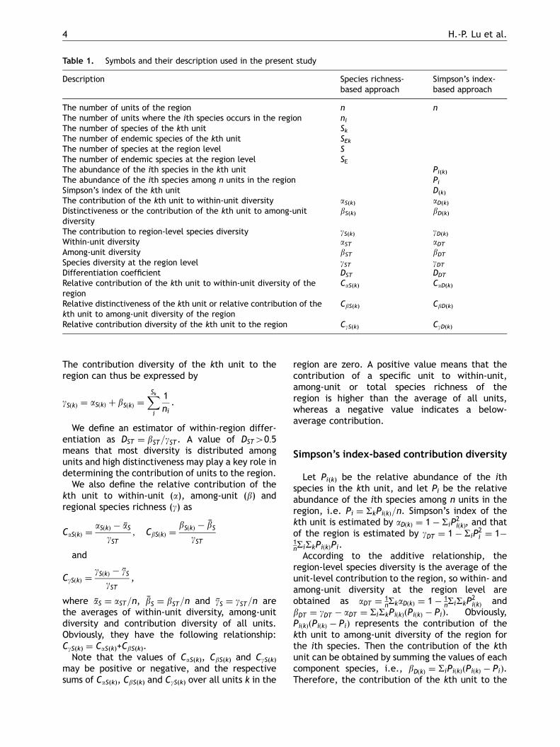
Table 1. Symbols and their description used in the present study

Description Species richness-based approach

Simpson’s index-based approach

The number of units of the region n nThe number of units where the ith species occurs in the region niThe number of species of the kth unit SkThe number of endemic species of the kth unit SEkThe number of species at the region level SThe number of endemic species at the region level SEThe abundance of the ith species in the kth unit Pi(k)The abundance of the ith species among n units in the region PiSimpson’s index of the kth unit D(k)

The contribution of the kth unit to within-unit diversity aS(k) aD(k)Distinctiveness or the contribution of the kth unit to among-unitdiversity

bS(k) bD(k)

The contribution to region-level species diversity gS(k) gD(k)Within-unit diversity aST aDTAmong-unit diversity bST bDTSpecies diversity at the region level gST gDTDifferentiation coefficient DST DDT

Relative contribution of the kth unit to within-unit diversity of theregion

CaS(k) CaD(k)

Relative distinctiveness of the kth unit or relative contribution of thekth unit to among-unit diversity of the region

CbS(k) CbD(k)

Relative contribution diversity of the kth unit to the region CgS(k) CgD(k)

H.-P. Lu et al.4

The contribution diversity of the kth unit to theregion can thus be expressed by

gSðkÞ ¼ aSðkÞ þ bSðkÞ ¼XSk

i

1ni.

We define an estimator of within-region differ-entiation as DST ¼ bST=gST. A value of DST40:5means that most diversity is distributed amongunits and high distinctiveness may play a key role indetermining the contribution of units to the region.

We also define the relative contribution of thekth unit to within-unit (a), among-unit (b) andregional species richness (g) as

CaSðkÞ ¼aSðkÞ � aS

gST; CbSðkÞ ¼

bSðkÞ � bSgST

and

CgSðkÞ ¼gSðkÞ � gS

gST,

where aS ¼ aST=n, bS ¼ bST=n and gS ¼ gST=n arethe averages of within-unit diversity, among-unitdiversity and contribution diversity of all units.Obviously, they have the following relationship:CgS(k) ¼ CaS(k)+CbS(k).

Note that the values of CaS(k), CbS(k) and CgS(k)

may be positive or negative, and the respectivesums of CaS(k), CbS(k) and CgS(k) over all units k in the

region are zero. A positive value means that thecontribution of a specific unit to within-unit,among-unit or total species richness of theregion is higher than the average of all units,whereas a negative value indicates a below-average contribution.

Simpson’s index-based contribution diversity

Let Pi(k) be the relative abundance of the ithspecies in the kth unit, and let Pi be the relativeabundance of the ith species among n units in theregion, i.e. Pi ¼ SkPiðkÞ=n. Simpson’s index of thekth unit is estimated by aDðkÞ ¼ 1� SiP

2iðkÞ, and that

of the region is estimated by gDT ¼ 1� SiP2i ¼ 1�

1nSiSkPiðkÞPi.

According to the additive relationship, theregion-level species diversity is the average of theunit-level contribution to the region, so within- andamong-unit diversity at the region level areobtained as aDT ¼ 1

nSkaDðkÞ ¼ 1� 1nSiSkP

2iðkÞ and

bDT ¼ gDT � aDT ¼ SiSkPiðkÞðPiðkÞ � PiÞ. Obviously,PiðkÞðPiðkÞ � PiÞ represents the contribution of thekth unit to among-unit diversity of the region forthe ith species. Then the contribution of the kthunit can be obtained by summing the values of eachcomponent species, i.e., bDðkÞ ¼ SiPiðkÞðPiðkÞ � PiÞ.Therefore, the contribution of the kth unit to the

ARTICLE IN PRESS

Contribution diversity to evaluate species diversity 5

species diversity of the region can be estimatedby gDðkÞ ¼ aDðkÞ þ bDðkÞ ¼ 1� SiPiðkÞPi. A Simpson’s index-based differentiation coefficient can bedefined as DDT ¼ bDT=gDT .

With these estimates, we can also characterizethe relative contribution of the kth unit to within-unit, among-unit and total species diversity of theregion by

CaDðkÞ ¼aDðkÞ � aD

ngDT; CbDðkÞ ¼

bDðkÞ � bDngDT

and

CgDðkÞ ¼gDðkÞ � gDngDT

.

The ecological meanings of these components arethe same as for the corresponding estimates in thespecies-richness approach.

Example data sets

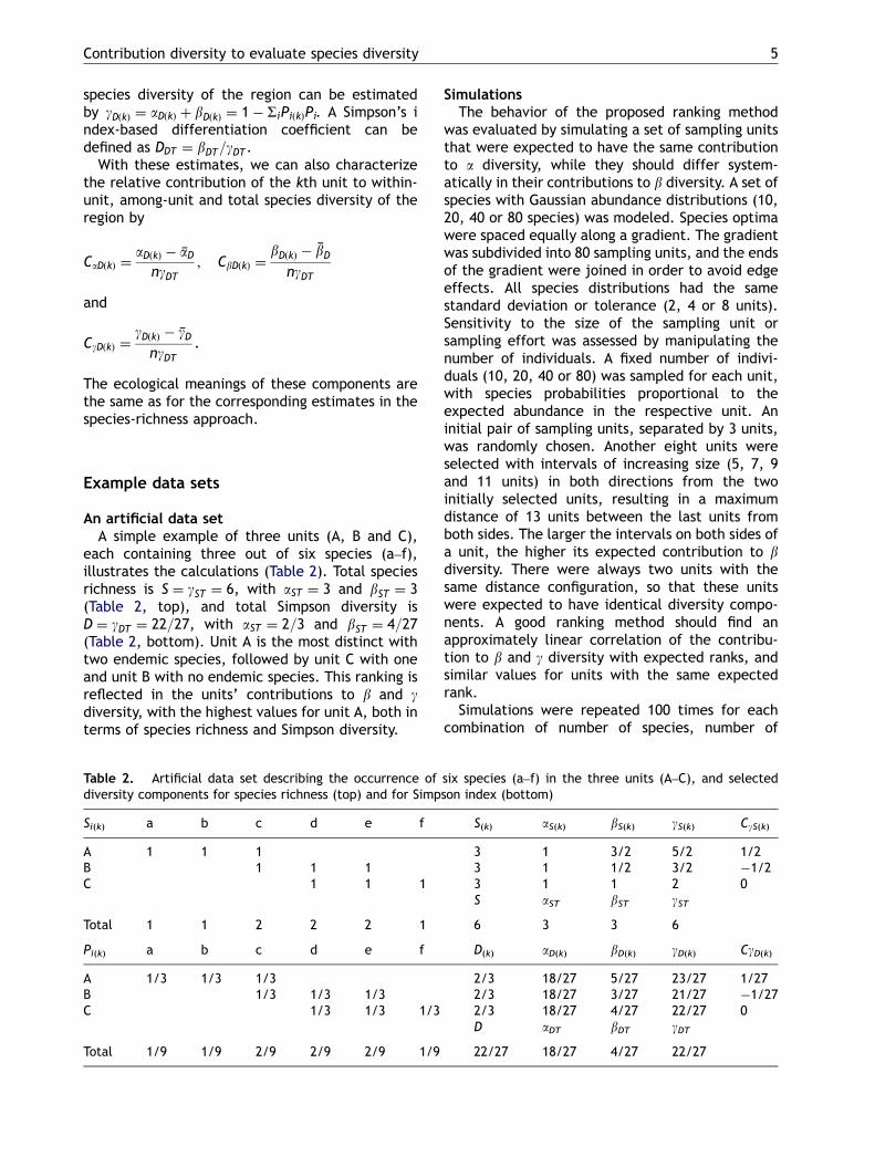
An artificial data setA simple example of three units (A, B and C),

each containing three out of six species (a–f),illustrates the calculations (Table 2). Total speciesrichness is S ¼ gST ¼ 6, with aST ¼ 3 and bST ¼ 3(Table 2, top), and total Simpson diversity isD ¼ gDT ¼ 22=27, with aST ¼ 2=3 and bST ¼ 4=27(Table 2, bottom). Unit A is the most distinct withtwo endemic species, followed by unit C with oneand unit B with no endemic species. This ranking isreflected in the units’ contributions to b and gdiversity, with the highest values for unit A, both interms of species richness and Simpson diversity.

Table 2. Artificial data set describing the occurrence ofdiversity components for species richness (top) and for Simp

Si(k) a b c d e f

A 1 1 1B 1 1 1C 1 1 1

Total 1 1 2 2 2 1

Pi(k) a b c d e f

A 1/3 1/3 1/3B 1/3 1/3 1/3C 1/3 1/3 1/3

Total 1/9 1/9 2/9 2/9 2/9 1/9

SimulationsThe behavior of the proposed ranking method

was evaluated by simulating a set of sampling unitsthat were expected to have the same contributionto a diversity, while they should differ system-atically in their contributions to b diversity. A set ofspecies with Gaussian abundance distributions (10,20, 40 or 80 species) was modeled. Species optimawere spaced equally along a gradient. The gradientwas subdivided into 80 sampling units, and the endsof the gradient were joined in order to avoid edgeeffects. All species distributions had the samestandard deviation or tolerance (2, 4 or 8 units).Sensitivity to the size of the sampling unit orsampling effort was assessed by manipulating thenumber of individuals. A fixed number of indivi-duals (10, 20, 40 or 80) was sampled for each unit,with species probabilities proportional to theexpected abundance in the respective unit. Aninitial pair of sampling units, separated by 3 units,was randomly chosen. Another eight units wereselected with intervals of increasing size (5, 7, 9and 11 units) in both directions from the twoinitially selected units, resulting in a maximumdistance of 13 units between the last units fromboth sides. The larger the intervals on both sides ofa unit, the higher its expected contribution to bdiversity. There were always two units with thesame distance configuration, so that these unitswere expected to have identical diversity compo-nents. A good ranking method should find anapproximately linear correlation of the contribu-tion to b and g diversity with expected ranks, andsimilar values for units with the same expectedrank.

Simulations were repeated 100 times for eachcombination of number of species, number of

six species (a–f) in the three units (A–C), and selectedson index (bottom)

S(k) aS(k) bS(k) gS(k) CgS(k)

3 1 3/2 5/2 1/23 1 1/2 3/2 �1/23 1 1 2 0S aST bST gST

6 3 3 6

D(k) aD(k) bD(k) gD(k) CgD(k)

2/3 18/27 5/27 23/27 1/272/3 18/27 3/27 21/27 �1/272/3 18/27 4/27 22/27 0D aDT bDT gDT

22/27 18/27 4/27 22/27

ARTICLE IN PRESS

H.-P. Lu et al.6

individuals, and tolerance. After each replicatesimulation, diversity components were calculated.Ranking performance was evaluated by the R2 oflinear regressions of the number of endemic speciesSEk and of the contributions to b and g diversity,bS(k) and gS(k), on the expected ranks.

A real data setWe illustrate the ecological application of the

proposed methods with data from a Castanopsisfargesii+Schima superba community, the localclimax vegetation type, in Tiantong National ForestPark (TNP), Zhejiang Province of China (Song &Wang, 1995). The community data (region) con-sisted of nine 400m2 plots (units) (see Appendix A).Each plot was further divided into sixteen 5� 5m2

subplots. Each individual with diameter at breastheight45 cm was recorded and measured. Pi(k) wasdefined as the relative importance value, which ismeasured as one-third of the sum of the relativeabundance, relative dominance and relative fre-quency, of species i in the pooled subplots of unit k.

Based on these data, we calculated a, b and gdiversity components for species richness andSimpson index using the proposed formulae. Tocompare with other measurements, we also calcu-lated unit specificity, Sajj (total specificity of theunit j) and Sj (relative specificity of the unit j)(Wagner & Edwards, 2001) and residuals of species–area curves based on species richness (RS) andendemic species (RE), respectively (Hobohm,2003). As all plots were of the same size, residualswere calculated as log S–log Smean for speciesrichness and log E�log Emean for endemic species.

To evaluate the ranking of the units, we alsoapplied the complementarity approach (Vane-Wright, Humphries, & Williams, 1991), which hasbeen widely used to identify areas of conservationpriority based on species richness. This is aniterative procedure that selects units in a step-wise manner, such that at each step the newlyselected unit includes the greatest number ofspecies not yet represented among selected units(Vane-Wright et al., 1991). All units are initiallyranked according by the number of species, and theunit with the highest number of species is chosenfirst. Once the first choice has been made, allspecies included within that unit are ignored. Thesecond area is then drawn from the taxonomiccomplement of the first–the unit with the highestnumber of remaining species. This algorithmicprocedure is repeated until all species are ac-counted for the total complement (Vane-Wrightet al., 1991).

Results

Simulation results

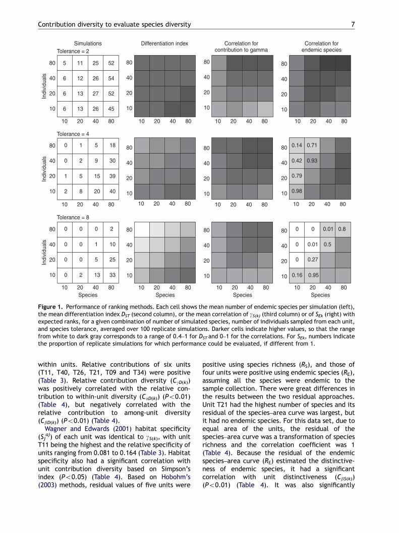
The sampled units differed much in speciescomposition and little in species richness, so thatgS(k) was highly correlated with bS(k) (r ¼ 0:97, onlygS(k) shown in Fig. 1, third column). The perfor-mance of the ranking methods depended stronglyon species tolerance, i.e., the standard deviationof simulated species distributions (Fig. 1, withincreasing tolerance from top to bottom row). Asexpected, the differentiation index (Fig. 1, secondcolumn) decreased with increasing tolerance, dueto an increasing overlap of species abundancedistributions along the gradient. However, smallsamples from species communities artificially in-creased DST. Narrow speciose distributions (Fig. 1,top row) resulted in high numbers of endemicspecies, leading to generally high linear correla-tions between the expected ranks and all threediversity measures. SEk (Fig. 1, last column)performed slightly better than gS(k), mostly becausethe latter was more sensitive to sample size. On theother hand, gS(k) was robust towards changes intolerance, whereas the performance of SEk de-creased strongly with increasing tolerance, espe-cially for large samples and few simulated species.Furthermore, SEk often could not be calculated atall in these situations.

Tiantong National Forest Park data

In the nine plots (units) of the Castanopsisfargesii+Schima superba community (region), gdiversity was 42, means of a and b diversity were13.22 and 28.78, respectively, based on speciesrichness (Table 3). The differentiation index wasDST ¼ 0:685, indicating that most diversity waspartitioned among units. Relative contributions offive units (T11, T21, T34, T01, and T40) werepositive, indicating that their contributions werelarger than the average. Relative contributiondiversity (CgS(k)) was significantly correlated withrelative unit distinctiveness (CbS(k)) (Po0.01) andhad a critically significant correlation with therelative contribution of within-unit diversity (CaS(k))(Po0.10) (Table 4). No significant correlation wasfound between relative contribution of within-unitdiversity (CaS(k)) and relative unit distinctiveness(CbS(k)).

The average of Simpson’s indices of the units was0.816, while Simpson’s index of the region was0.883. The differentiation index was DDT ¼ 0:077,indicating that most diversity was partitioned

ARTICLE IN PRESS

10

20

40

80

10

20

40

80

10 20 40 80

10

20

40

80

Differentiation index

10

20

40

80

10 20 40 80

Correlation forcontribution to gamma

10 20 40 80

0.98

0.79

0.42 0.93

0.14 0.71

10

20

40

80

10

20

40

80

10

20

40

80

Species10 20 40 80 10 20 40 80

Species

0.16 0.95

0 0.27

0 0.01 0.5

0 0 0.01 0.8

10 20 40 80

10

20

40

80

Indi

vidu

als

2 8 20 40

1 5 15 39

0 2 9 30

0 1 5 18

Tolerance = 4

Indi

vidu

als

Tolerance = 8

10 20 40 80

10

20

40

80

Species

0 2 13 33

0 0 5 25

0 0 1 10

0 0 0 2

Tolerance = 2Simulations

10 20 40 80

10

20

40

80

Indi

vidu

als

6 13 26 45

6 13 27 52

6 12 26 54

5 11 25 52

10 20 40 80

10

20

40

80

10 20 40 80

10 20 40 80Species

10 20 40 80

10

20

40

80

Correlation forendemic species

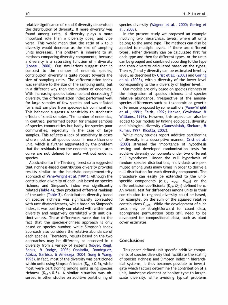
Figure 1. Performance of ranking methods. Each cell shows the mean number of endemic species per simulation (left),the mean differentiation index DST (second column), or the mean correlation of gS(k) (third column) or of SEk (right) withexpected ranks, for a given combination of number of simulated species, number of individuals sampled from each unit,and species tolerance, averaged over 100 replicate simulations. Darker cells indicate higher values, so that the rangefrom white to dark gray corresponds to a range of 0.4–1 for DST and 0–1 for the correlations. For SEk, numbers indicatethe proportion of replicate simulations for which performance could be evaluated, if different from 1.

Contribution diversity to evaluate species diversity 7

within units. Relative contributions of six units(T11, T40, T26, T21, T09 and T34) were positive(Table 3). Relative contribution diversity (CgD(k))was positively correlated with the relative con-tribution to within-unit diversity (CaD(k)) (Po0.01)(Table 4), but negatively correlated with therelative contribution to among-unit diversity(CbD(k)) (Po0.01) (Table 4).

Wagner and Edwards (2001) habitat specificity(Sj

aj) of each unit was identical to gS(k), with unitT11 being the highest and the relative specificity ofunits ranging from 0.081 to 0.164 (Table 3). Habitatspecificity also had a significant correlation withunit contribution diversity based on Simpson’sindex (Po0.05) (Table 4). Based on Hobohm’s(2003) methods, residual values of five units were

positive using species richness (RS), and those offour units were positive using endemic species (RE),assuming all the species were endemic to thesample collection. There were great differences inthe results between the two residual approaches.Unit T21 had the highest number of species and itsresidual of the species–area curve was largest, butit had no endemic species. For this data set, due toequal area of the units, the residual of thespecies–area curve was a transformation of speciesrichness and the correlation coefficient was 1(Table 4). Because the residual of the endemicspecies–area curve (RE) estimated the distinctive-ness of endemic species, it had a significantcorrelation with unit distinctiveness (CbS(k))(Po0.01) (Table 4). It was also significantly

ARTICLE IN PRESS

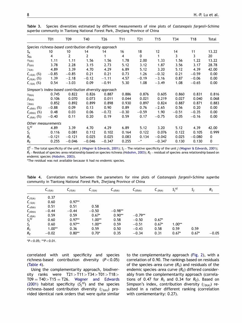
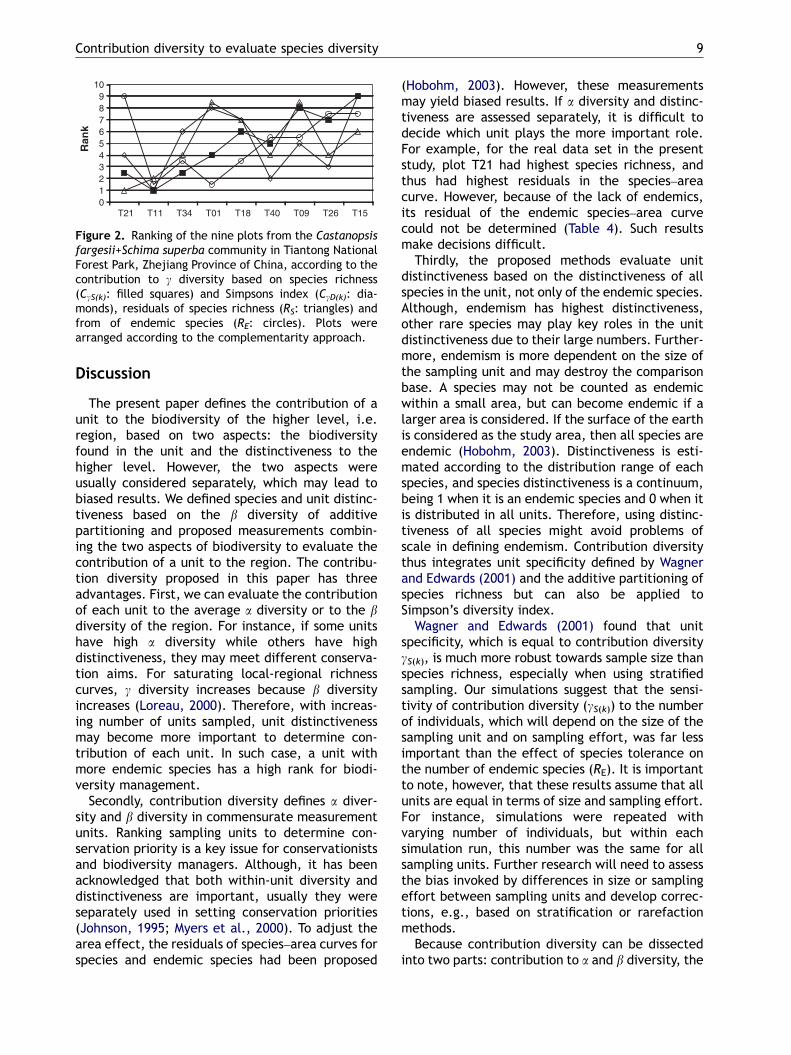
Table 3. Species diversities estimated by different measurements of nine plots of Castanopsis fargesii+Schimasuperba community in Tiantong National Forest Park, Zhejiang Province of China

T01 T09 T40 T26 T11 T21 T15 T34 T18 Total

Species richness-based contribution diversity approachSk 10 10 14 14 16 18 12 14 11 13.22SEk 4 2 2 1 4 0 1 3 3 20aS(k) 1.11 1.11 1.56 1.56 1.78 2.00 1.33 1.56 1.22 13.22bS(k) 3.78 2.28 3.15 2.73 5.12 3.12 1.87 3.56 3.17 28.78gS(k) 4.89 3.39 4.70 4.29 6.89 5.12 3.20 5.12 4.39 42.00CaS(k) (%) �0.85 �0.85 0.21 0.21 0.73 1.26 �0.32 0.21 �0.59 0.00CbS(k) (%) 1.39 �2.18 �0.12 �1.11 4.57 �0.19 �3.16 0.87 �0.06 0.00CgS(k) (%) 0.54 �3.03 0.09 �0.91 5.30 1.08 �3.49 1.08 �0.65 0.00

Simpson’s index-based contribution diversity approachaD(k) 0.745 0.822 0.826 0.887 0.886 0.876 0.605 0.860 0.831 0.816bD(k) 0.106 0.070 0.073 0.011 0.044 0.021 0.219 0.027 0.040 0.068gD(k) 0.852 0.892 0.899 0.898 0.930 0.897 0.824 0.887 0.871 0.883CaD(k) (%) �0.88 0.09 0.13 0.90 0.89 0.76 �2.65 0.56 0.20 0.00CbD(k) (%) 0.48 0.03 0.06 �0.72 �0.30 �0.59 1.90 �0.51 �0.35 0.00CgD(k) (%) �0.40 0.11 0.20 0.19 0.59 0.17 �0.75 0.05 �0.16 0.00

Other measurementsSj

aj 4.89 3.39 4.70 4.29 6.89 5.12 3.20 5.12 4.39 42.00Sj 0.116 0.081 0.112 0.102 0.164 0.122 0.076 0.122 0.105 0.999RS �0.121 �0.121 0.025 0.025 0.083 0.134 �0.042 0.025 �0.080 0RE 0.255 �0.046 �0.046 �0.347 0.255 —* �0.347 0.130 0.130 0

Sajj – The total specificity of the unit j (Wagner & Edwards, 2001); Sj – The relative specificity of the unit j (Wagner & Edwards, 2001);RS – Residual of species–area relationship based on species richness (Hobohm, 2003); RE – residual of species–area relationship based onendemic species (Hobohm, 2003).*The residual was not available because it had no endemic species.

Table 4. Correlation matrix between the parameters for nine plots of Castanopsis fargesii+Schima superbacommunity in Tiantong National Forest Park, Zhejiang Province of China

CaS(k) CbS(k) CgS(k) CaD(k) CbD(k) CgD(k) Sjaj Sj RS

CbS(k) 0.37CgS(k) 0.60 0.97**CaD(k) 0.51 0.51 0.58CbD(k) �0.44 �0.44 �0.50 �0.98**CgD(k) 0.59 0.59 0.67* 0.90** �0.79**Sj

aj 0.60 0.97** 1.00** 0.58 �0.50 0.67*Sj 0.60 0.97** 1.00** 0.59 �0.51 0.67* 1.00**RS 1.00** 0.36 0.59 0.50 �0.43 0.58 0.59 0.59RE �0.02 0.80** 0.70* 0.35 �0.34 0.31 0.67* 0.67* �0.05

*Po0.05; **Po0.01.

H.-P. Lu et al.8

correlated with unit specificity and speciesrichness-based contribution diversity (Po0.05)(Table 4).

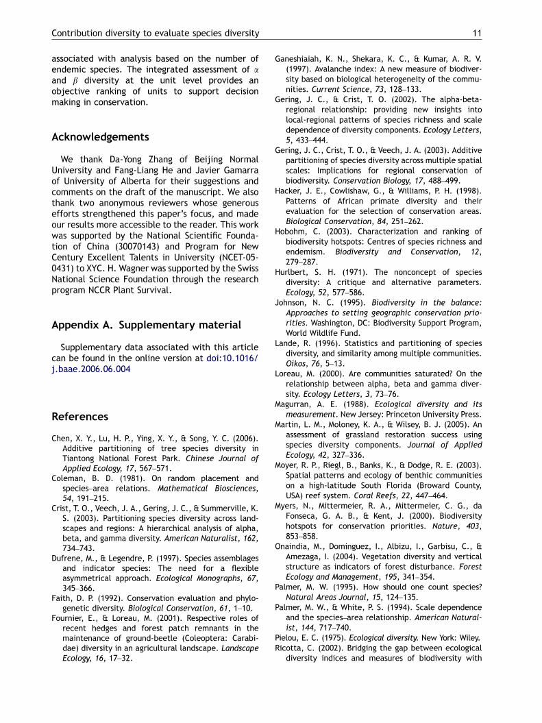
Using the complementarity approach, biodiver-sity ranks were T214T114T344T014T184T09 ¼ T404T15 ¼ T26. Wagner and Edwards(2001) habitat specificity (Sj

aj) and the speciesrichness–based contribution diversity (gS(k)) pro-vided identical rank orders that were quite similar

to the complementarity approach (Fig. 2), with acorrelation of 0.90. The rankings based on residualsof the species–area curve (RS) and residuals of theendemic species–area curve (RE) differed consider-ably from the complementarity approach (correla-tions of 0.47 for RS and 0.34 for RE). Based onSimpson’s index, contribution diversity (gD(k)) re-sulted in a rather different ranking (correlationwith comlementarity: 0.27).

ARTICLE IN PRESS

0123456789

10

T21 T11 T34 T01 T18 T40 T09 T26 T15

Ran

k

Figure 2. Ranking of the nine plots from the Castanopsisfargesii+Schima superba community in Tiantong NationalForest Park, Zhejiang Province of China, according to thecontribution to g diversity based on species richness(CgS(k): filled squares) and Simpsons index (CgD(k): dia-monds), residuals of species richness (RS: triangles) andfrom of endemic species (RE: circles). Plots werearranged according to the complementarity approach.

Contribution diversity to evaluate species diversity 9

Discussion

The present paper defines the contribution of aunit to the biodiversity of the higher level, i.e.region, based on two aspects: the biodiversityfound in the unit and the distinctiveness to thehigher level. However, the two aspects wereusually considered separately, which may lead tobiased results. We defined species and unit distinc-tiveness based on the b diversity of additivepartitioning and proposed measurements combin-ing the two aspects of biodiversity to evaluate thecontribution of a unit to the region. The contribu-tion diversity proposed in this paper has threeadvantages. First, we can evaluate the contributionof each unit to the average a diversity or to the bdiversity of the region. For instance, if some unitshave high a diversity while others have highdistinctiveness, they may meet different conserva-tion aims. For saturating local-regional richnesscurves, g diversity increases because b diversityincreases (Loreau, 2000). Therefore, with increas-ing number of units sampled, unit distinctivenessmay become more important to determine con-tribution of each unit. In such case, a unit withmore endemic species has a high rank for biodi-versity management.

Secondly, contribution diversity defines a diver-sity and b diversity in commensurate measurementunits. Ranking sampling units to determine con-servation priority is a key issue for conservationistsand biodiversity managers. Although, it has beenacknowledged that both within-unit diversity anddistinctiveness are important, usually they wereseparately used in setting conservation priorities(Johnson, 1995; Myers et al., 2000). To adjust thearea effect, the residuals of species–area curves forspecies and endemic species had been proposed

(Hobohm, 2003). However, these measurementsmay yield biased results. If a diversity and distinc-tiveness are assessed separately, it is difficult todecide which unit plays the more important role.For example, for the real data set in the presentstudy, plot T21 had highest species richness, andthus had highest residuals in the species–areacurve. However, because of the lack of endemics,its residual of the endemic species–area curvecould not be determined (Table 4). Such resultsmake decisions difficult.

Thirdly, the proposed methods evaluate unitdistinctiveness based on the distinctiveness of allspecies in the unit, not only of the endemic species.Although, endemism has highest distinctiveness,other rare species may play key roles in the unitdistinctiveness due to their large numbers. Further-more, endemism is more dependent on the size ofthe sampling unit and may destroy the comparisonbase. A species may not be counted as endemicwithin a small area, but can become endemic if alarger area is considered. If the surface of the earthis considered as the study area, then all species areendemic (Hobohm, 2003). Distinctiveness is esti-mated according to the distribution range of eachspecies, and species distinctiveness is a continuum,being 1 when it is an endemic species and 0 when itis distributed in all units. Therefore, using distinc-tiveness of all species might avoid problems ofscale in defining endemism. Contribution diversitythus integrates unit specificity defined by Wagnerand Edwards (2001) and the additive partitioning ofspecies richness but can also be applied toSimpson’s diversity index.

Wagner and Edwards (2001) found that unitspecificity, which is equal to contribution diversitygS(k), is much more robust towards sample size thanspecies richness, especially when using stratifiedsampling. Our simulations suggest that the sensi-tivity of contribution diversity (gS(k)) to the numberof individuals, which will depend on the size of thesampling unit and on sampling effort, was far lessimportant than the effect of species tolerance onthe number of endemic species (RE). It is importantto note, however, that these results assume that allunits are equal in terms of size and sampling effort.For instance, simulations were repeated withvarying number of individuals, but within eachsimulation run, this number was the same for allsampling units. Further research will need to assessthe bias invoked by differences in size or samplingeffort between sampling units and develop correc-tions, e.g., based on stratification or rarefactionmethods.

Because contribution diversity can be dissectedinto two parts: contribution to a and b diversity, the

ARTICLE IN PRESS

H.-P. Lu et al.10

relative significance of a and b diversity depends onthe distribution of diversity. If more diversity wasfound among units, b diversity plays a moreimportant role than a diversity does, and viceversa. This would mean that the ratio of a to bdiversity would decrease as the size of samplingunits increases. This problem is inherent to allmethods comparing diversity components, becausea diversity is a saturating function of g diversity(Loreau, 2000). Our simulations suggest that incontrast to the number of endemic species,contribution diversity is quite robust towards thesize of sampling units. The differentiation indexwas sensitive to the size of the sampling units, butin a different way than the number of endemics.With increasing species tolerance and decreasing bdiversity, the differentiation index performed wellfor large samples of few species and was inflatedfor small samples from species-rich communities.This behavior suggests a sensitivity to stochasticeffects of small samples. The number of endemics,in contrast, performed better for smaller samplesof species communities but badly for species-poorcommunities, especially in the case of largesamples. This reflects a lack of sensitivity in caseswhere most or all species occur in more than oneunit, which is further aggravated by the problemthat the residuals from the endemic species - areacurve are not defined for units without endemicspecies.

Application to the Tiantong forest data suggestedthat richness-based contribution diversity providesresults similar to the heuristic complementarityapproach of Vane-Wright et al.(1991). Although thecontribution diversity of each unit based on speciesrichness and Simpson’s index was significantlyrelated (Table 4), they produced different rankingsof the units (Table 3). Contribution diversity basedon species richness was significantly correlatedwith unit distinctiveness, while based on Simpson’sindex, it was positively correlated with within-unitdiversity and negatively correlated with unit dis-tinctiveness. These differences were due to thefact that the species-richness approach is onlybased on species number, while Simpson’s indexapproach also considers the relative abundance ofeach species. Therefore, results based on the twoapproaches may be different, as observed in adiversity from a variety of systems (Moyer, Riegl,Banks, & Dodge, 2003; Onaindia, Dominguez,Albizu, Garbisu, & Amezaga, 2004; Song & Wang,1995). In fact, most of the diversity was partitionedwithin units using Simpson’s index (DDTo0.5), whilemost were partitioning among units using speciesrichness (DST40.5). A similar situation was ob-served in other studies on additive partitioning of

species diversity (Wagner et al., 2000; Gering etal., 2003).

In the present study we proposed an exampleinvolving two hierarchical levels, where all unitsbelong to the same type. The methods can also beapplied to multiple levels. If there are differenttypes, either diversity can be calculated first foreach type and then for different types, or the unitscan be grouped and combined according to the typeand then diversity calculated based on the types.Then a, b and g diversity can be estimated level bylevel, as described by Crist et al. (2003) and Geringet al. (2003), with g diversity of the lower levelcorresponding to the a diversity of higher level.

Our models are only based on species richness orthe integration of species richness and speciesrelative abundance, irrespective of the among-species differences such as taxonomic or geneticdifferences proposed by some authors (Vane-Wrightet al., 1991; Faith, 1992; Hacker, Cowlishaw, &Williams, 1998). However, this aspect can also beadded to our models by linking ecological diversityand biological diversity (Ganeshiaiah, Shekara, &Kumar, 1997; Ricotta, 2002).

While many studies report additive partitioningof diversity in a descriptive manner, Crist et al.(2003) stressed the importance of hypothesistesting and developed randomization tests foradditive diversity components under two differentnull hypotheses. Under the null hypothesis ofrandom species distributions, individuals are per-muted among units many times in order to derive anull distribution for each diversity component. Theprocedure can easily be extended to the unit-specific components (e.g., aS(k), bS(k)) or thedifferentiation coefficients (DST, DDT) defined here.An overall test for differences among units in theircontribution to regional diversity could be based,for example, on the sum of the squared relativecontributions CgS(k). While the development of suchtests may be straightforward for count data,appropriate permutation tests still need to bedeveloped for compositional data, such as plantcover estimates.

Conclusions

This paper defined unit-specific additive compo-nents of species diversity that facilitate the scalingof species richness and Simpson index in hierarch-ical systems. It thus becomes possible to investi-gate which factors determine the contribution of aunit, landscape element or habitat type to larger-scale diversity, while avoiding typical problems

ARTICLE IN PRESS

Contribution diversity to evaluate species diversity 11

associated with analysis based on the number ofendemic species. The integrated assessment of aand b diversity at the unit level provides anobjective ranking of units to support decisionmaking in conservation.

Acknowledgements

We thank Da-Yong Zhang of Beijing NormalUniversity and Fang-Liang He and Javier Gamarraof University of Alberta for their suggestions andcomments on the draft of the manuscript. We alsothank two anonymous reviewers whose generousefforts strengthened this paper’s focus, and madeour results more accessible to the reader. This workwas supported by the National Scientific Founda-tion of China (30070143) and Program for NewCentury Excellent Talents in University (NCET-05-0431) to XYC. H. Wagner was supported by the SwissNational Science Foundation through the researchprogram NCCR Plant Survival.

Appendix A. Supplementary material

Supplementary data associated with this articlecan be found in the online version at doi:10.1016/j.baae.2006.06.004

References

Chen, X. Y., Lu, H. P., Ying, X. Y., & Song, Y. C. (2006).Additive partitioning of tree species diversity inTiantong National Forest Park. Chinese Journal ofApplied Ecology, 17, 567–571.

Coleman, B. D. (1981). On random placement andspecies–area relations. Mathematical Biosciences,54, 191–215.

Crist, T. O., Veech, J. A., Gering, J. C., & Summerville, K.S. (2003). Partitioning species diversity across land-scapes and regions: A hierarchical analysis of alpha,beta, and gamma diversity. American Naturalist, 162,734–743.

Dufrene, M., & Legendre, P. (1997). Species assemblagesand indicator species: The need for a flexibleasymmetrical approach. Ecological Monographs, 67,345–366.

Faith, D. P. (1992). Conservation evaluation and phylo-genetic diversity. Biological Conservation, 61, 1–10.

Fournier, E., & Loreau, M. (2001). Respective roles ofrecent hedges and forest patch remnants in themaintenance of ground-beetle (Coleoptera: Carabi-dae) diversity in an agricultural landscape. LandscapeEcology, 16, 17–32.

Ganeshiaiah, K. N., Shekara, K. C., & Kumar, A. R. V.(1997). Avalanche index: A new measure of biodiver-sity based on biological heterogeneity of the commu-nities. Current Science, 73, 128–133.

Gering, J. C., & Crist, T. O. (2002). The alpha-beta-regional relationship: providing new insights intolocal-regional patterns of species richness and scaledependence of diversity components. Ecology Letters,5, 433–444.

Gering, J. C., Crist, T. O., & Veech, J. A. (2003). Additivepartitioning of species diversity across multiple spatialscales: Implications for regional conservation ofbiodiversity. Conservation Biology, 17, 488–499.

Hacker, J. E., Cowlishaw, G., & Williams, P. H. (1998).Patterns of African primate diversity and theirevaluation for the selection of conservation areas.Biological Conservation, 84, 251–262.

Hobohm, C. (2003). Characterization and ranking ofbiodiversity hotspots: Centres of species richness andendemism. Biodiversity and Conservation, 12,279–287.

Hurlbert, S. H. (1971). The nonconcept of speciesdiversity: A critique and alternative parameters.Ecology, 52, 577–586.

Johnson, N. C. (1995). Biodiversity in the balance:Approaches to setting geographic conservation prio-rities. Washington, DC: Biodiversity Support Program,World Wildlife Fund.

Lande, R. (1996). Statistics and partitioning of speciesdiversity, and similarity among multiple communities.Oikos, 76, 5–13.

Loreau, M. (2000). Are communities saturated? On therelationship between alpha, beta and gamma diver-sity. Ecology Letters, 3, 73–76.

Magurran, A. E. (1988). Ecological diversity and itsmeasurement. New Jersey: Princeton University Press.

Martin, L. M., Moloney, K. A., & Wilsey, B. J. (2005). Anassessment of grassland restoration success usingspecies diversity components. Journal of AppliedEcology, 42, 327–336.

Moyer, R. P., Riegl, B., Banks, K., & Dodge, R. E. (2003).Spatial patterns and ecology of benthic communitieson a high-latitude South Florida (Broward County,USA) reef system. Coral Reefs, 22, 447–464.

Myers, N., Mittermeier, R. A., Mittermeier, C. G., daFonseca, G. A. B., & Kent, J. (2000). Biodiversityhotspots for conservation priorities. Nature, 403,853–858.

Onaindia, M., Dominguez, I., Albizu, I., Garbisu, C., &Amezaga, I. (2004). Vegetation diversity and verticalstructure as indicators of forest disturbance. ForestEcology and Management, 195, 341–354.

Palmer, M. W. (1995). How should one count species?Natural Areas Journal, 15, 124–135.

Palmer, M. W., & White, P. S. (1994). Scale dependenceand the species–area relationship. American Natural-ist, 144, 717–740.

Pielou, E. C. (1975). Ecological diversity. New York: Wiley.Ricotta, C. (2002). Bridging the gap between ecological

diversity indices and measures of biodiversity with

ARTICLE IN PRESS

H.-P. Lu et al.12

Shannon’s entropy: Comment to Izsak and Papp.Ecological Modelling, 152, 1–3.

Ricotta, C. (2003). Additive partition of parametricinformation and its associated beta-diversity measure.Acta Biotheoretica, 51, 91–100.

Ricotta, C. (2005). A note on functional diversitymeasures. Basic and Applied Ecology, 6, 479–486.

Song, Y. C., & Wang, X. R. (1995). Vegetation and flora ofTiantong national forest park, Zhejiang province.Shanghai: Shanghai Scientific Documentary Press.

Stendera, S. E. S., & Johnson, R. K. (2005). Additivepartitioning of aquatic invertebrate species diversityacross multiple spatial scales. Freshwater Biology, 50,1360–1375.

Vane-Wright, R. I., Humphries, C. J., & Williams, P. H.(1991). What to protect? Systematics and the agony ofchoice. Biological Conservation, 55, 235–254.

Veech, J. A. (2000). Choice of species–area functionaffects identification of hotspots. Conservation Biol-ogy, 14, 140–147.

Veech, J. A., Summerville, K. S., Crist, T. O., & Gering,J. C. (2002). The additive partitioning of speciesdiversity: Recent revival of an old idea. Oikos, 99,3–9.

Wagner, H. H., & Edwards, P. J. (2001). Quantifyinghabitat specificity to assess the contribution of a patchto species richness at a landscape scale. LandscapeEcology, 16, 121–131.

Wagner, H. H., Wildi, O., & Ewald, K. C. (2000). Additivepartitioning of plant species diversity in an agricultur-al mosaic landscape. Landscape Ecology, 15, 219–227.

Whittaker, R. H. (1960). Vegetation of the siskiyoumountains, Oregon and California. Ecological Mono-graphs, 30, 279–338.