Embed Size (px)
DESCRIPTION
A Continuum Theory of Elastic Material Surfaces
Citation preview

A Continuum Theory of Elastic Material Surfaces
MORTON E. GURTIN & A. IAN MURDOCH
Abstract
A mathematical framework is developed to study the mechanical behavior of material surfaces. The tensorial nature of surface stress is established using the force and moment balance laws. Bodies whose boundaries are material surfaces are discussed and the relation between surface and body stress examined. Elastic surfaces are defined and a linear theory with non-vanishing residual stress derived. The free-surface problem is posed within the linear theory and uniqueness of solution demonstrated. Predictions of the linear theory are noted and compared with the corresponding classical results. A note on frame-indifference and symmetry for material surfaces is appended.
Table of Contents
I n t roduc t i on . . . . . . . . . . . . . . . . . . . . . . . . . . . . . . . . . . . . 291 1. P r e l i m i n a r y Def in i t ions . . . . . . . . . . . . . . . . . . . . . . . . . . . . . 293 2. Surfaces . . . . . . . . . . . . . . . . . . . . . . . . . . . . . . . . . . . . 294 3. K i n e m a t i c s . . . . . . . . . . . . . . . . . . . . . . . . . . . . . . . . . . . 299 4. Bodies. M a t e r i a l Surfaces. Interfaces . . . . . . . . . . . . . . . . . . . . . . . . 300 5. Surface Stress . . . . . . . . . . . . . . . . . . . . . . . . . . . . . . . . . . 301 6. E q u i l i b r i u m for T h r e e - D i m e n s i o n a l Bodies wi th M a t e r i a l Bounda r i e s . . . . . . . . . . 307 7. E las t ic Surfaces . . . . . . . . . . . . . . . . . . . . . . . . . . . . . . . . . 310 8. L inear ized T h e o r y . . . . . . . . . . . . . . . . . . . . . . . . . . . . . . . . 313 9. L inear ized T h e o r y of a B o d y wi th a F ree Surface . . . . . . . . . . . . . . . . . . . 314
10. S imple A p p l i c a t i o n s of the L inea r T h e o r y . . . . . . . . . . . . . . . . . . . . . . 319 10.1. Inf ini te Cy l ind r i ca l Surface B o u n d i n g a H o m o g e n e o u s I so t rop ic Body . . . . . . . 319 10.2. P l a n e Waves in a Hal f -Space . . . . . . . . . . . . . . . . . . . . . . . . . 320
A p p e n d i x . . . . . . . . . . . . . . . . . . . . . . . . . . . . . . . . . . . . . 321 References . . . . . . . . . . . . . . . . . . . . . . . . . . . . . . . . . . . . . 323
Introduction
As is well known, 1 surfaces of bodies and interfaces between pairs of bodies exhibit properties quite different from those associated with their interiors. While the literature on surface phenomena is extensive, 2 it is based, for the most part, on molecular considerations. In spite of the importance of surface phenomena, with the exception of some isolated work on fluid films 3 and on the thermodynamics of
t Cf . , e.g., ADAM (1941) and ADAMSON (1967). 2 Cf. , e.g., the h is tor ica l b a c k g r o u n d out l ined by OROWAN (1970). There the con t r i bu t i ons of
YOUNG, LAPLACE, Gmas , and others are discussed. 3 Cf. , e.g., S c R r v ~ (1960).
21 Arch. Rat. Mech. Anal., Vol. 57
292 M.E . GURTIN & A. I. MURDOCH
non-deformable interfaces, 1 there does not exist a systematic treatment 2 of material surfaces based on the modem ideas now prevalent in continuum mechan- ics. That such an approach is valid and of use in the understanding of surface phenomena has been cogently argued by HERRING. 3 In this paper we present a first step towards the development of a rational theory of material surfaces.
Section 1 is concerned with preliminary definitions and notation, while Section 2 develops a general theory of surfaces in Euclidean space. In Section 3 we study the deformation of surfaces and introduce the relevant measures of strain. Section 4 is devoted to a careful definition of the notion of a material surface; roughly speaking, a material surface is defined as a two-dimensional continuous body embedded in a Euclidean space of dimension three. What we believe is a radically new view of the boundary surface of a three-dimensional body is also presented in Section 4 together with a precise definition for the interface between two continuous bodies. Here we are concerned with modelling transition zones between immiscible materials and do not consider diffusion; thus phase interfaces do not fall within the scope of our theory. Surface stress is introduced in Section 5 and its tensorial nature (Cauchy's Theorem) is established, in the usual manner, with the aid of the force and moment balance laws. Here, of course, the ideas are the same as those underlying the classical theory of membranes. 4 We feel, however, that the modem geometric concepts used allow for a more precise and compact theory. In Section 6 we study the consequences of equilibrium for a body whose boundary is a material surface. In particular, we deduce interesting relations be- tween the stress field associated with the body and that associated with the boundary surface. Section 7 is concerned with the only constitutive class we presently consider: that of an elastic surface. Here we study, in the usual manner, 5 the consequences of frame-indifference and material symmetry. In Section 8 we deduce a linearized theory of elastic surfaces. A novel feature of this theory is the linearized stress-strain relation giving the surface stress tensor as a residual stress tensor plus a linear function of surface strain. 6 This obviously generalizes the usual notion of surface tension and is, in fact, consistent with atomistic calcula- tions indicating the presence of compressive surface stresses in certain c r y s t a l s . 7
Section 9 deals with the formulation of the free-surface problem within the linear theory. This problem models situations, for example, in which a part of a body is removed, thereby exposing a free surface. Thus, while the interior of the body may be initially free of stress, the residual surface stress in the boundary surface generates a stress field in the body. Predictions of the linear theory in several simple cases are noted in Section 10 and compared with the corresponding classical results.
1 FISHER (~ LEITMAN (1968); WILLIAMS (1972). 2 Of COurse, there do exist various ad hoc theories, such as the theory of fracture, in which cracks
are allowed to have surface tension, but in which the effect of this surface tension on the strain field in the body is ignored. In this connection see the remarks by GOODIER (1968), p. 21.
3 HERRING (1953).
4 Cf., e.g., TRUESDELL (g~ TOUPIN (1960) and NAGHDI (1972). 5 Cf, e.g., TRUESDELL t~ NOLL (1965). 6 C f the remarks of HERRING (1953). 7 SHUTTLEWORTH (1950). See also LENNARD-JoNm & DENT (1928), LENNARD-JONm (1930),
OROWAN (1932).

Elastic Material Surfaces 293
1. Preliminary Definitions
Let ~ / and ~ r designate finite-dimensional inner product spaces, and let
U n i t ( ~ ) = t h e set of all unit vectors in q/, Lin(q/, ~fr)= the space of linear transformations from q/ in to
Invlin(~, ~ r ) = {FeLin(r ~C): F is invertible}.
(Of course, Invlin(q/, ~/C) is empty when dim o//4= dim ~.) We write S T for the transpose of SeLin(q/, ~/~)~ so that STeLin(~C, ~/) and
w . S u = S r w . u
for every ueq/, we~r (We use the same symbol "-" for the inner product on any finite-dimensional inner product space; the underlying space will always be clear from the context.) We say that SeLin(r o//) is symmetric i f S = S r, positive- definite if u4:0 implies u .Su>O. For SeLin(q/, o//), trS and detS denote, respec- tively, the trace and determinant of S, and the inner product on Lin(~, ~r is defined by
U . F = tr (UF r)
for all U, F e Lin(q/, ~r Let dim q / = d i m ~.. Then QeLin(~ ~r) is orthogonal if
Q r Q = the ident i tyon ~ ,
Q Q r = t h e identity on ~ .
Given vectors u e q/, we ~ we define u | w e Lin(~r,, o//) by
(u | a = ( w . a ) u
for every a e ~/r and, when u, we ~r
UAW=U|174
We will consistently use the following notation:
Sym(~) = {Se Lin(O//, ://): S is symmetric}, Sym + (q/)= {SeSym(qQ: S is positive-definite},
Orth(~, ~/:)= {QeLin(~ , ~/:): Q is orthogonal}, Unim(~) = {UeLin(q/, ~) : det U = -t- 1}.
We now state, without proof, the following slightly generalized version of the polar decomposition theorem: 1
Theorem 1.1. Each F e Invlin(~, ~t:) admits the unique decomposition
F = R U (1.1)
with U e S y m + (~/)and ReOrth(q/, ~r). Moreover
U 2 = FTF. (1.2)
I Cf., e.g., HALMOS (1958), p. 169. 21"
294 M.E. GURTIN (g: A. I. MURDOCH
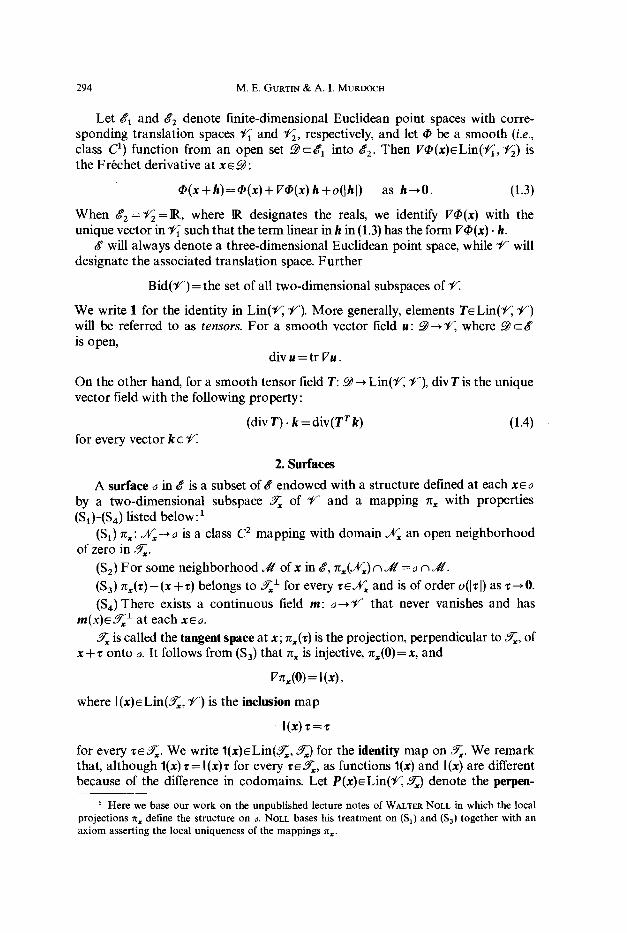
Let 81 and 8 2 denote finite-dimensional Euclidean point spaces with corre- sponding translation spaces ~ and V22, respectively, and let q, be a smooth (i.e., class C 1) function from an open set ~ c 8 1 into gz. Then V~(x)~Lin(~ , ~2) is the F r6chet derivative at x ~ ~ :
�9 ( x+h)=~(x )+ lTr as h ~ 0 . (1.3)
When ~ 2 = ~ = ~ , where IR designates the reals, we identify V~(x) with the unique vector in ~ such that the term linear in h in (1.3) has the form V~(x). h.
will always denote a three-dimensional Euclidean point space, while ~e- will designate the associated translation space. Further
B i d (~ ) = the set of all two-dimensional subspaces of ~.
We write 1 for the identity in Lin(~,, ~r). More generally, elements T~Lin(~,, ~ ) will be referred to as tensors. For a smooth vector field u: ..@~V, where ~ c & is open,
div u = tr Vu.
On the other hand, for a smooth tensor field T: ~ ~ Lin(~,, ~ ) , div T is the unique vector field with the following property:
(div T)- k = div(T T k) (1.4)
for every vector k 6 ~ .
2. Surfaces
A surface 0 in o ~ is a subset ofo ~ endowed with a structure defined at each x~o by a two-dimensional subspace ~ of C and a mapping rr x with properties (S1)-(S,) listed below: 1
(St) nx: J f f ~ o is a class C 2 mapping with domain JV~ an open neighborhood of zero in ~ .
($2) For some neighborhood Jg of x in d ~, rr~(Jff~)n ~ / = 0 c~ J / .
($3) 7z~(~)-(x + ~) belongs to ~ • for every ~eJff~ and is of order o(l~ I) as ~ 0.
(S,) There exists a continuous field m: 0--,~/r that never vanishes and has r a ( x ) e ~ • at each x~o.
is called the tangent space at x; rt~(~) is the projection, perpendicular to ~ , of x +~ onto o. It follows from ($3) that 7z~ is injective, 7zx(0)= x, and
v ~ . ( 0 ) = I (x) ,
where I(x)~ L i n ( ~ , ~/:) is the inclusion map
I(x)~=~
for every ~ e ~ . We write l (x )~L in (~ , ~ ) for the identity map on ~ . We remark that, al though l (x )~= I(x)~ for every ~ , as functions l(x) and I(x) are different because of the difference in codomains. Let P(x)~Lin(~,, ~ ) denote the perpen-
Here we base our work on the unpublished lecture notes of WALTER NOLL in which the local projections n~ define the structure on ~. NOLL bases his treatment on (S 0 and ($3) together with an axiom asserting the local uniqueness of the mappings n~.
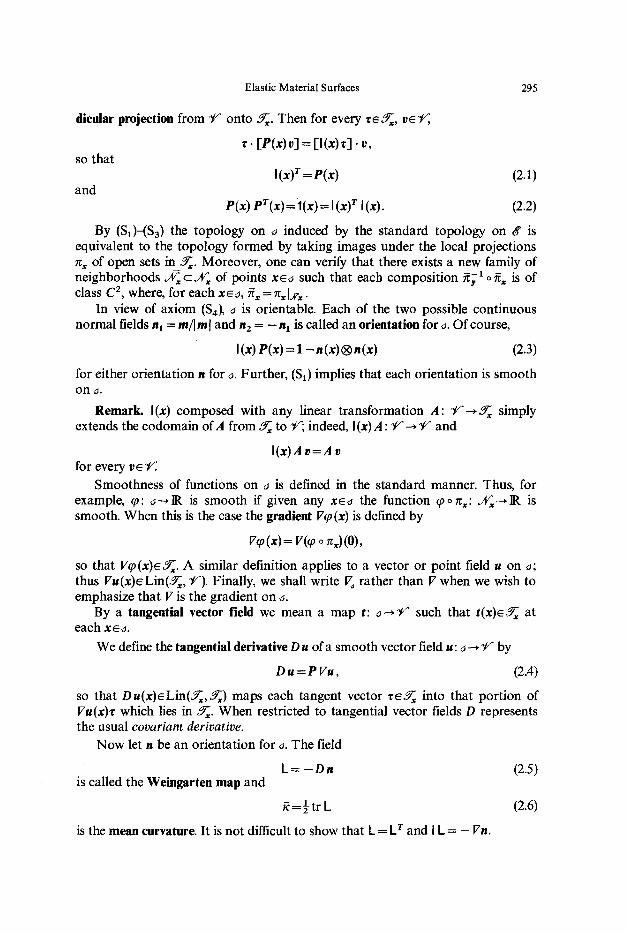
Elastic Material Surfaces 295
dicular projection from ~e" onto ~ . Then for every ~ , t~e ~r,,
�9 . I F ( x ) v] = [ l ( x ) ~ ] �9 v , so that
I (x )T=p(x) and
(2.1)
P(x) pT(x) =~I(x) = ' (X) T I(X). (2.2)
By ($I)-($3) the topology on o induced by the standard topology on g is equivalent to the topology formed by taking images under the local projections rcx of open sets in ~r x. Moreover, one can verify that there exists a new family of neighborhoods J ~ C J ~ x of points x~o such that each composit ion ~ - I o fix is of class C 2, where, for each x ~ , ~x = rq, l~,,.
In view of axiom ($4), a is orientable. Each of the two possible continuous normal fields n~ = m/[ m l and n2 = - n l is called an orientation for o. Of course,
I(x) V(x) = I - n (x) | n(x) (2.3)
for either orientation n for o. Further, (Sx) implies that each orientation is smooth on o.
Remark. I(x) composed with any linear transformation A: ~v ' - - .~ simply extends the codomain of,4 from ~ to ~v; indeed, I (x) A : ~v'---, ~ and
[ ( x ) A v = A v for every v ~ .
Smoothness of functions on o is defined in the standard manner. Thus, for example, q~: o - - ,R is smooth if given any x~o the function q~orc~: J f f ~ R is smooth. When this is the case the gradient Vq~ (x) is defined by
v ~ (x) = v(~0 o ~ ) (0),
so that V~o(x)e~. A similar definition applies to a vector or point field u on o; thus IZu(x)eLin(~d~x, ~v~). Finally, we shall write ~ rather than 17 when we wish to emphasize that I z is the gradient on ~.
By a tangential vector field we mean a map t: o ~ v " such that t ( x ) e ~ at each x ~ o.
We define the tangential derivative D u of a smooth vector field u: o--* ~v by
D u = P Vu, (2.4)
so that D u ( x ) 6 L i n ( ~ , ~ ) maps each tangent vector , E ~ into that portion of Vu(x)r which lies in ~ . When restricted to tangential vector fields D represents the usual covariant derivative.
Now let n be an orientation for o. The field
L = - D n (2.5) is called the Weingarten map and
= �89 tr I_ (2.6)
is the mean curvature. It is not difficult to show that L = L r and I L = - 17n.
296 M.E. GURTIN & A. I. MURDOCH
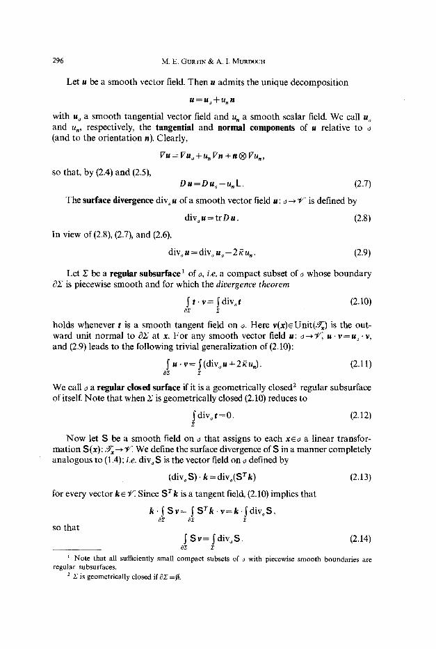
Let u be a smoo th vector field. Then u admits the unique decompos i t ion
U = U ~ + U n n
with u~ a smoo th tangential vector field and u, a smoo th scalar field. We call u o and u,, respectively, the tangential and normal components of u relative to o (and to the or ienta t ion n). Clearly,
Vu = Vuo + u, Vn + n | Vu,,
so that, by (2.4) and (2.5), D u = D u ~ - u . L . (2.7)
The surface divergence divo u of a smoo th vector field u: o ~ ~e" is defined by
divo u = t rD u. (2.8)
In view of (2.8), (2.7), and (2.6),
div~ u = divo u o - 2 ~ u.. (2.9)
Let Z be a regular subsurface 1 of o, i.e. a compac t subset of o whose bounda ry BZ is piecewise smoo th and for which the divergence theorem
t . v = ~ divot (2.10) O2 ,~
holds whenever t is a smooth tangent field on o. Here v ( x ) e U n i t ( ~ ) is the out- ward unit no rma l to OZ at x. F o r any smoo th vector field u: o ~ , , u . v = u ~ .v, and (2.9) leads to the following trivial general izat ion of (2.10):
u . v = ~ (div~ u + 2 ~ u , ) . (2.11) 02 2
We call o a regular closed surface if it is a geometr ical ly closed 2 regular subsurface of itself. No te that when Z is geometr ical ly closed (2.10) reduces to
div~ t = 0 . (2.12)
N o w let S be a smoo th field on o that assigns to each x e o a linear t ransfor- ma t ion $ (x): ~ ~ ~ . We define the surface divergence of $ in a manne r complete ly ana logous to (1.4); i.e. divo 5 is the vector field on o defined by
(div~ 5 ) . k = divo(Sr k) (2.13)
for every vector k ~ . Since 5 r k is a tangent field, (2.10) implies that
k . ~ S v = ~ 5 r k - v = k . ~ d i v o 5 ,
so tha t 5 v = ~ d ivo5 . (2.14)
0f
Note that all sufficiently small compact subsets of o with piecewise smooth boundaries are regular subsurfaces.
2 27 is geometrically closed if 02: =~.

Elastic Material Surfaces 297
A tangential tensor field is a field T on o that assigns to each x~o a linear transformation T(x): ~ ~ ~ . Examples of tangential tensor fields are 1, L, and D u. The above definition of the divergence cannot be used for such a field T, since T r k is defined only for k e ~ . However, since I(x)T(x): ~ f , , $ = IT is a field of the type discussed in the previous paragraph, and we can define
div~ T = div~(I T), (2.15)
or equivalently, by (2.13),
(div, T)- k = d i v ~ ( T r p k )
for every k e ~. Then, if we replace S in (2.14) by I T and use the fact that I T v = T v, we are led to the conclusion that
T v = ~ divo T. (2.16)
The following useful identities can be proved in the same way as their more familiar counterparts:
V(u . v )=(Vu) r v + ( V v ) r u ,
V@ u)=~o Vu + u | V~o ,
divo(q~ u)=q~ divo u + u. IZgo, (2.17)
divo(q~ $)=~0 divo $ + $ Vq~,
divo(S T u) = (div~ $) . u + S . Vu,
where qh u, v, and S are smooth fields on o with ~0 scalar-valued, u and v vector- valued, and S(x)eLin(o~, ~/r). If T is a smooth tangential tensor field, then (2.17)4 and (2.17)s with S = IT yield, on use of (2.15),
div,@ T)=rp divo T + Y Vrp,
div~(Tr pu )=(d i vo T) �9 u + T . Du. (2.18)
Further, (2.18)2 with u = n and (2.5) imply that
(divo Y)- n = T- I_. (2.19)
Proposition 2.1. div, 1 = divo I =2~n . (2.20)
Proof. F o r any k~oe we have
(div, 1). k = (divo I). k = div,(Pk) = div, (k - (n. k) n) = (n. k) 2 ~,
as is clear from (2.15) with T = 1, (2.13), (2.1), (2.3), (2.17)3, and (2.9). D
In addition to the above identities, the following lemma will be useful.
Lemma 2.1. Let S be a smooth tensor f ield on ~ with S(x)ELin(~-~, ~ ) , and let u be a smooth vector f ie ld on ~. Then
S S v | S [div~ S | + S Fur]. (2.21)

298 M.E. GURTIN & A. I. MURDOCH
Further, u | ~ [u | $ + Vu S t ] ,
u ^ S v = ~ [ u ^ d i v ~ S + V u S r - S V u r ] , 05 Z
u. S v= I [(divo S)" u + S" Vu].
Proof. For every ke3e ~ we have
(2.22)
on using (2.14). implies that
( I $ v | u) k = I (u- k) S v = ~ divo ((u. k) S),
However, if we note that V(u.k)=(Fu)rk by (2.17) 1, (2.17)4
I div~((u �9 k)S)= I [(u. k) div, $ + S [7urk] ={~ [(div~ $) | u + S Fur]} k,
which yields the proof of (2.21). The operators on Lin(~,, "U) which deliver the transpose, skew part, and trace are linear and continuous and, when applied to a| have values b| �89 ^b, and a . b, respectively. Thus, if we apply these operators to both sides of(2.21), we are led, at once, to equations (2.22). D
A curve 7 on ~ is a subset ofo with the following property: 7 is the range of a smooth one-to-one mapping from [0, 1] into 6. We write 171 for the length of 7. An oriented curve is a curve 7 together with a choice of unit normal field v to 7; v is then called the positive unit normal field for 7. (A unit normal field v for 7 is a continuous vector field on 7 such that, for each xe 7, v(x)e Unit(~) is perpendicular to 7 at x. Of course, each curve 7 has exactly two such unit normal fields.) A curve 7' c 7 is an oriented subcurve of 7 if the positive unit normal fields to 7' and 7 coincide on 7'.
Definitions analogous to the above apply to curves in 4 . In particular, if 7 is an oriented curve in ~ , we denote by 7" the image of 7 under n~; 7~ is assumed to have the orientation induced by nx. We shall omit the subscript x when the underlying tangent space ~ is clear from the context. If 7 is parametrized by f : [0, 1 ] ~ , then 7" is parametrized by ~ o f : [13, 1]--*~, and a simple compu- tation leads to the inequality
[17"1 -I~,1 [ s sup {1Vnx(~; 1 ( r ) ) - I(x)[} 171. (2.23)
Given xea, we write ~r for the family of all line segments in ~ having ve Unit(G) as positive unit normal, and, for TeXx,
~q~ T)= {Ee 5('~(v): TEE}. (2.24)
Let A~ (e > 0) be a one-parameter'family of subsets of 6. We say that A, tends to xeo if, given any neighborhood X of x in a, there is an e0>0 such that A ~ c Y for all e < eo.
Let Z, (e > 13) be a one-parameter family of area-measurable sets in ~ such that 2;* =n~(Z3 tends to x. Then, since ~ is the tangent space at x, it is not difficult

Elas t i c Ma te r i a l Surfaces 299
to verify that I area(Z*)- area(Z~)l ~ 0 as e--}0. (2.25)
3. Kinematics
Let Diff(8) denote the set of all class C 2 diffeomorphisms of 8 onto itself. Let % be a surface in 6". By a deformation of 6o (into 6) we mean a mapping f : %--+6, where ~ is a surface in ~f, such that f=gl~o with g~Diff(8). Let Jx ~ X~6o, and ~ , x~o, designate the tangent spaces to ~o and ~, respectively, and let
F= Vf, (3.1)
so that F(X)~Lin(3"x ~ ~) .
Proposition 3.1. For each X~ 6 o the linear transformation F(X) has range in ~ , where x = f (X). Further, if we let F(X) denote F(X) considered as a linear transfor- mation with ~ as codomain, then F(YOs Invlin(fx ~ ~~).
The field F is called the deformation gradient corresponding to f. The above proposition and Theorem 1.1 imply that F has the polar decomposition
F = R U (3.2)
with U(X)~Sym+(Jx ~ and R(X)~Orth(~x~ The tensor U(X) is called the right stretch tensor at X. For all vectors u, VSSx ~
(F rFu).v=Fu- Fv=Fu- Fv=(FrFu).v, so that, by (1.2),
U 2 : F r F = ~r ~. (3.3)
The displacement u: ~o ~ f/" corresponding to f is defined by
u ( X ) = f ( X ) - X . Then, clearly,
Vu = g - I, (3.4)
where I(X): ~x~ e" is the inclusion map of the tangent space to 6o at X. By (3.3), (3.4), (2.1), (2.2) and (2.4),
U 2 =1 +2 E + Vu r Vu, (3.5)
where I(X) is the identity on Jx ~ and
E =�89 u +D ur). (3.6)
The tangential tensor field E is called the infinitesimal strain; E is important in theories based on the approximative assumption that IZu be small. By (2.7) and the symmetry of L,
E = �89 Uoo + D UYo) - u. L, (3.7) 1
where k is the Weingarten map on 6o, and where uoo and u, are, respectively, the tangential and normal components of u relative to %.
1 Cf., e.g., NAGHDI (1972), (6.18) 1 .

300 M.E. GURTIN & A. I. MURDOCH
Now let geDiff(o ~) be given by g(X) = Zo + Fo(X- Xo), (3.8)
where Xo, Zor and Fo~Invlin(~,,~). Then o=g(%) is a surface in g, and fo =gl~o is a deformation of ~o into ~. A deformation fo of this form is called a homogeneous deformation of ~o into a.
Proposition 3.2. Let ~r and let Fr ~ q/). ?hen there exists a homogeneous deformation fo of ~o whose deformation gradient at X is F.
Proof. Let nl and n2 be unit vectors with n ~ x ~177 and n2~q/• let
be defined by Fo ~ Invlin(~,, C)
Fou=Fu, u~Jx ~
F o U l = n 2 ,
and let g: o ~ o ~ be given by (3.8) with Xo, Zo arbitrary. Then the corresponding homogeneous deformation fo has F as deformation gradient at X. rq
4. Bodies. Material Surfaces. Interfaces
We begin by defining a body 1 in sufficient generality to include the notion of a material surface. A body is a set IB with a structure defined by a family �9 of configurations subject to the following axioms:
(i) each K~C is an injection oflB into 8;
(ii) if !r and f ~ Diff(o~), then f Is(s) o r ~ C; (iii) if r, F-~ C, then there exists an fE Diff(8) such that F o K- t = f Is(m).
The elements XelB are called material points, and the sets rOB ) ( reC) images of IB. Let IBo cIB. Then lBo equipped with the family
Co={~l~o: ~ } is also a body; 113o is called a subbody of IB. Two bodies 1131 and IB2 are compatible if IB1 u 1132 can be endowed with the structure of a body in such a way that IB1 and IBz are subbodies oflB1 ulBz.
A material surface is a body 6P whose images are all surfaces. We will con- sistently write ~x(x) for the tangent space to the surface x(Se) at the point X = to(X); ~x(K) is called the tangent space at X in x.
A three-dimensional body is a body ~ whose images are closures of bounded z open sets in 8. For such a body ~ is the subset of ~ with the property that K(d~)=t3(K(~)) in some (and hence every) configuration x. We say that ~ has a material boundary if ~3~ is a material surface.
Let ~ and ~2 be compatible three-dimensional bodies. Then Se = ~1 c~ ~2 is the interface between ~1 and ~2 provided ~ as a subbody of ~ u ~z, is a material surface.
1 Cf. NOEL (1973), p. 70. 2 We assume ~ is bounded to avoid repeated regularity assumptions concerning the behavior
of the relevant fields at infinity. In Section 10, where we apply our theory, this assumption is tacitly dropped.
Elastic Material Surfaces 301
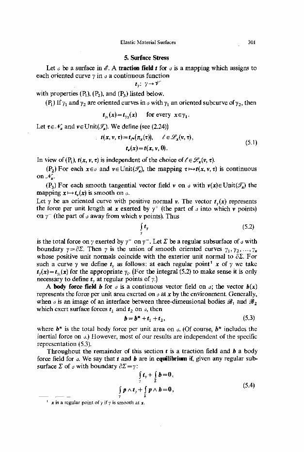
5. Surface Stress
Let 6 be a surface in 8. A traction field t for 6 is a mapping which assigns to each oriented curve 2) in ~ a continuous function
t~: 2)---, V
with properties (P1), (P2), and (P3) listed below.
(P1) If 2)1 and 2)2 are oriented curves in 6 with 2)1 an oriented subcurve of 2)2, then
tT~(x)=t~2(x ) for every x~2)1.
Let z ~ ~ and w Unit (~-:). We define (see (2.24))
t(x, v, ~)=t~.(~x(~)), :~ex(v, ~), (5.1)
t~(x)=t(x, v, 0).
In view of (P1)~ t(x, v, ~) is independent of the choice o f : 6 Lax(v, ~).
(P2) For each x66 and v6Unit(~v~), the mapping ~--, t(x, v, ~) is continuous o n ,~x .
(P3) For each smooth tangential vector field v on 6 with v (x )~Uni t (~ ) the mapping x~-+t~(x) is smooth on 6. Let 2) be an oriented curve with positive normal v. The vector tr(x) represents the force per unit length at x exerted by 3, + (the part of 6 into which v points) on 2)- (the part of 6 away from which v points). Thus
?
is the total force on 2) exerted by 2)+ on 2)-. Let Z be a regular subsurface of 6 with boundary 2)= dZ. Then 2) is the union of smooth oriented curves 71,2)2 . . . . . 2), whose positive unit normals coincide with the exterior unit normal to ~E. For such a curve 2) we define t v as follows: at each regular point 1 x of 2) we take tr(x)=tv,(x ) for the appropriate ?i. (For the integral (5.2) to make sense it is only necessary to define t r at regular points of 2).)
A body force field b for 6 is a continuous vector field on a; the vector b(x) represents the force per unit area exerted on 6 at x by the environment. Generally, when a is an image of an interface between three-dimensional bodies ~1 and ~2 which exert surface forces tl and t2 on 6, then
b = b* + t l + t 2 , (5.3)
where b* is the total body force per unit area on 6. (Of course, b* includes the inertial force on 6.) However, most of our results are independent of the specific representation (5.3).
Throughout the remainder of this section t is a traction field and b a body force field for 6. We say that t and b are in eqmlibrium if, given any regular sub- surface Z of ~ with boundary dE = 2):
~t~+~b=O, 7 s
p ^ t~ + y p ^ b = 0, (5.4)
x is a regular poin t of ? if ? is s m o o t h at x.

302 M. E. GURTIN & A. I. MURDOCH
where p ( x ) = x - Xo (5.5)
is the position vector from an arbitrary fixed point Xo.
Theorem 5.1. Let t and b be in equilibrium. Then tr(x) depends on y only through the positive unit normal v to 7 at x. In fact, given x~6 and veUni t (~ ) ,
tr(x)=tv(X) (5.6)
for every oriented curve 7 in o which passes through x and whose positive unit normal f ield takes the value v at x.
The proof of this theorem is based on the following three lemmas. The first is a direct consequence of the continuity of t r on 7; the second follows from (P2), (2.23), and (5.1)2; the third is a consequence of (2.25) and the continuity of b on 6.
Lemma 5.1. Let ~ be an oriented curve in 6, and let ?~ (e > O) be a one-parameter family of oriented subcurves of y such that 7~ tends to x ~6 as e ~ O. Then
tv=lT, Itv(x)+o(17,l) as e ~ O . Y~
Lemma 5.2. Let vr Further, let f~ (e>0) be a one-parameter family of line segments with f ~6 ~x(v), and suppose that f ~ tends to x~6 as e ~O. Then
t .--141 tv(x)+o(l<l) as 5 0. r
LemmaS.3. Let x66, and let r,~ (5>0) be a one-parameter family of area- measurable sets in ~ such that ~,* = nx(2~) tends to x as e~O. Then
b=O(Area(Z )) as -o0.
Proof of Theorem 5.1. In what follows it is often convenient to identify the tangent space ~ with the tangent plane at x by means of the correspondence x*--~x+r for every ~ 6 ~ . We shall generally make no distinction between the tangent space and tangent plane; it will always be clear from the context which is intended. Our first step will be to prove that
iv(x)= (5.7)
for every w U n i t ( ~ ) . Thus choose such a v and consider the rectangle R~ in centered at x with sides of length e and e6 (e > 0, c5 > 0) and with the sides of length eft parallel to v. Clearly, for sufficiently small e, R,6Jff~ and, further, R* = n~(R,) as well as each of its sides tends to x as e ~ 0 . Thus if we apply (5.4)1 to R*, divide the resulting equation by e, and let e ~ 0 , we conclude with the aid of Lemmas 5.2 and 5.3 that
t~ (x) + t_~(x) + 6 {t~(x) + t_,(x)} = 0,
where r e U n i t ( ~ ) and v- r =0. Since 6 is arbitrary, this clearly implies (5.7).
Now let ? be an oriented curve on 6 whose positive unit normal at x is v, and let F be a segment of the tangent line to 7 at x, lying within Jff~, including x, and having orientation opposite to that of 7 at x. Then F e o ~ ( - v , O ) and, by

Elastic Mater ia l Surfaces 303
(5.1) and (5.7), tr,(x)= -tv(x).
Thus, to complete the proof, it clearly suffices to prove that
-tr,(x). (5.8) With this in mind, let
so that 7' is that curve in JV~ which corresponds, under the diffeomorphism nx, to that part of 7 lying in the range of ~ . If 7 and F* coincide in a neighborhood of x, then (near x) 7' must be a line segment through x with orientation opposite to that of F, and (5.8) follows at once from (5.7). Thus we assume that ~ and F* differ in every neighborhood of x. Then locally at x in ~ we shall have, for a sub- segment of F, one of the two situations in Figure 1.
Case (i). Choose y on F with I x - y l = e and zeT' with z - y perpendicular to F. Let E~ denote the line segment from y to z, and let ~', and F~ denote, respectively, those parts of 7 and F which with g~ form a curvilinear triangle 27, with vertices x, y, and z. Further, let ~ be equipped with the orientation corresponding to the outward normal to 27~. Then ~*, ~*, and 7~ = rc~(7',) form the boundary of the region 2~* =rc~(27,) in 6, and therefore, since t and b are in equilibrium, (5.4)1 applied to 27* yields
S tet + ~ tr, + I tr + I b = 0. (5.9)
Clearly, Z*, g*, F~*, and ~,~ each tend to x as ~ 0 . Further, since F~ and 7'~ are tangent at x, it follows that IF~I =~, I~'~l =IF~I +o(~), It~l =o(~), and Area(27~)= o(~ 2)
1,.' - M
- ~ , ( i ) ~, (ii)
Fig, 1
- v
- ' b '
Fig. 2 "12 Fig. 3

304 M. E. GURTIN & A. I. MURDOCH
as e~0. Thus if we divide (5.9) by e and let e~0, we conclude, with the aid of Lemmas 5.1-5.3, that
tr(x)+tr,(x)=O,
which is the desired result (5.8).
Case (ii). For this case we must choose another curvilinear triangle in ~M~ before (5.4)1 can be applied. This time Z~ is the curvilinear triangle with vertices at x, y' and z, where [ x - y ' I = l y - z [ and x - y ' is perpendicular to x - y . With F~ the line segment from y' to z furnished with unit normal -v , and f~ the line seg- ment from x to y' furnished with the outward normal to Z,, a completely anal- ogous analysis leads once again to (5.8). D
Theorem 5.2. Let t and b be in equilibrium. Then there exists a smooth symmetric tangential tensor field T such that
tv (x)=r(x)v (5.10)
for every v~ Uni t (d) and every x ~ o. Further
divo T + b = 0 .
Proof. We begin by defining "l~(x, .) on ~ by
(5 .11) 1
with T(x, v) : Ivl tv(x)
v=v/Ivl for v+0 .
(5.12)
If we set ~'(x, 0)=0, it is a simple matter, by use of (5.7), to show that
T(x, 2v)=2T(x, v) (5.13)
for every v ~ and every real number 2. We now show that 1"(x, "): ~ - ~ " is linear; i.e.,
T(x, " )~Lin(~ , U). (5.14)
By virtue of (5.13) it suffices to show additivity on linearly independent vectors. Thus let u, v ~ be linearly independent and construct a triangle in ~ with sides of lengths ~lul, ~lvl, and ~lu+vl having outward normals u,v, and -(u+v), respectively, and with x as circum-center. If we denote this triangle by A~, it is clear that, for small enough e, A, will lie in Jff~. Since Area(A,)=O(e z) as e~O, and since A* =zcx(A~) and each of its (curvilinear) sides tends to x as e~0 , if we apply (5.4)1 to A* and use Lemmas 5.2 and 5.3 we arrive at
~lul'~(x,u/lul)+~lvl$(x,v/Ivl)+elu+vl'~(x,-(u+v)/lu+vl)=o(e) as e~O.
Dividing by e, letting e--*0, and using (5.13) yields
$ (x, u) + ' t (x, v ) - ~ (x, (u + v))=0,
so that ~'(x, ") is additive on linearly independent vectors and (5.14) holds.
Cf, e.g., TRU~SDELL & TOUPIN (1960), Eq. (212.6) 1 .

Elastic Mater ia l Surfaces 305
We now write T(x, v)= T(x) v (5.15)
for all v e ~ , so that t ( x ) e L i n ( ~ , f ) . In view of (5.6), (5.12), and (5.15), the balance laws (5.4)1 and (5.4)2 now take
the forms S / ' v + S b = 0 ,
l p ^ , t v + l p ^ b = O , (5.16) 0s s
where v is the outward unit normal to OZ. By (P3) the mapping x ~ ?(x) is smooth on a. Thus (5.16)1 and the divergence theorem imply that
(di% ? + b) = 0
for every regular subsurface Z, and therefore, in the usual manner, the continuity of divo T and b yield the local relation
di% ~" + b =0 . (5.17)
Next let 2; be an arbitrary regular subsurface of ~. Since V ( x - Xo) = Izrrx(O) = I (x), (2.1) and (5.5) yield (vp)r=P, and (2.22)2 (with u = p and $ = I ) implies that
I P ^ T v = I ( p ^ d i v o T + p r T r - ' ~ P ) .
If we use (5.16)2 and (5.17), we arrive at the relation
I ( p r ~ r _ I" P)=O; X
hence
The remainder (2.1) and (2.2). Choose n e ~ x. Then, since "l~(x): ~ , (5.18) implies that
~ r n = I t r n = Pr ' i ' r n ='f 'Pn = 0
(where, for convenience, we have suppressed the argument x). Thus
n . "p v='pr n . v=O
for every v ~ , so that the range of ~'(x) lies in 4 . Therefore, if we let
T =P ' I ~, (5.19)
so that T is a smooth tangential tensor field on a, it follows that
"t = I r . (5.20) Thus
T v = T v
for every v ~ ; hence (5.12) and (5.15) imply (5.10). On the other hand, (5.20) and the definition of the divergence of a tangential tensor field yield (5.11). Thus, to
"[" p =p r ' ~ r . (5.18)
of the proof will make repeated use (without mention) of

306 M.E . GURTIN & A. I. MURDOCH
complete the proof, we have only to show that T is symmetric. By (5.18) and (5.19),
T = T p p r = p ' r p p r = p p r ' t r p r = ~ r p r = T r,
and the proof is complete. [q
For the remainder of this section we assume that t and b are in equilibrium. The symmetric tangential tensor field T, defined in Theorem 5.2, is called the surface stress.
Theorem 5.3. The surface stress T and the body force b satisfy the relation 1
T-L=-b.,
where b, = b . n with n a choice of unit normal f ield for ~ and L is the corresponding Weingarten map (2.5).
Proof. The result is immediate on using (2.19) and (5.11). D
We say that T is a surface tension a if a is a smooth scalar field on o and
T = a l .
Theorem 5.4. Let T be a surface tension a. Then
Vtr= -b~ ; 2~ t r= -bn ,
where b~ and b n are, respectively, the tangential and normal components of b.
Proof. By (5.11), (2.18), with q~ =cr and T =1, and (2.20)
V t r + 2 ~ a n + b = O .
The desired conclusions follow from this relation and the fact that Vtr is a tangential vector field. 0
Theorem 5.4 has an important corollary when o is (an image of) the interface between two three-dimensional bodies ~1 and ~2. Indeed, in the absence of inertial forces on 6, and when the forces exerted by &l and ~2 on o are derived from (not necessarily constant) pressures px and P2, then b in (5.3) is given by
b = (Pl - P2) n .
Here, of course, n is the outward unit normal to ~1 in the configuration under consideration. This should serve to motivate
Corollary 5.5. I f T is a surface tension a, and if b = (Pl - P2) n, then a is constant and
2 ~tr =P2 - P l . (5.21)
The equation (5.21) is usually referred to as Laplace's formula. 2 We remark that Theorem 5.3 is a generalized version of this relation.
In applications T represents the stress field in the current configuration of a material surface 6 a undergoing deformation. More precisely, if / l is such a con-
t C f . , e.g., TRUESDELL ~; TOUPIN (1960), Eq. (212.22)2.
2 Cf . , e.g . , LANDAU & LIFSHITZ (1959), w 60.

Elas t i c M a t e r i a l Su r f aces 307
figuration with/1(6e)=6, then for any xe6 and any unit vector v ~ ( / 0 , T(x)v is the force per unit length at x on any oriented curve ~ in 6 passing through x and having v as its positive unit normal at x. Let r be a second configuration of 6a and let f =/~ o ~ - 1 denote the corresponding deformation of 6o = ~(5 a) into 6 =/~(Sa). Then there exists a unique smooth field S on 6o with S(X)~ Lin(9-x(g), ~ ) such that
Sv o =~Tv (5.22) Yo y
for every oriented curve 7o in %, provided 7=f(7o) and v0 and v are, respectively, the positive unit normal fields for 7o and 7- S is called the Piola-Kirehhoff stress in/~ relative to x; by (5.22), Svo is the force per unit length of 7o. If F denotes the deformation gradient o f f , it may be shown that 1
(det U) (F - 1)r VO = j V, (5.23)
where U is the right stretch tensor field and j is the Radon-Nikodym derivative of the arc length measure on 7 with respect to that on 70. Equations (5.22) and (5.23) imply that
S (X) = (det U (X)) I ( f (X)) T ( f (X)) ( F (X)-I) r, (5.24)
where I(x) is the inclusion map of ~(/~) into ~. In view of(2.1) and (2.2),
T=(de t U ) - I P S F r ,
where P(x)=l(x) r is the perpendicular projection of ~ onto ~(p) , and where, for convenience, we have omitted arguments. Thus, since T takes symmetric values, S must satisfy
PSFT=FSrl. Let
where x=f(X), so that bo(X) = [det U(X)] b(x),
S bo=S b f - t ( ~ )
for any regular subsurface Z of o. Then balance of forces (5.16)1 is equivalent to the requirement that
Svo+ ~ bo=0 d,~o ~o
for every regular subsurface 2, o of Oo with vo the outward unit normal to a2; o. The divergence theorem together with the continuity of both divoo S and bo therefore yield the local form
divoo S + bo =0 . (5.25)
6. Equilibrium for Three-Dimensional Bodies with Material Boundaries
Let ~ be a three-dimensional body with a material boundary 5 a = a~, and let B=/K&) be the image of ~ in a configuration/~. If n denotes the outward unit normal field to OB, we take tl, the force per unit area exerted on 0B by the material
1 C f , e.g., TRUESDELL (1966), (11.12).
22 Arch. Rat. Mech. Anal., Vol. 57

308 M . E . GURTIN & A. I. MURDOCH
in/~ (the interior of B) to be given by
ti= - T n ,
where T is the continuous extension to dB of the Cauchy stress in/3. The body force field b on the image surface ~ =/~(6 e) is then given by (cf. (5.3))
b = b * - T n + t e ,
where b* is the inertial force per unit area and te is the force per unit area exerted on dB by the environment. Thus, if the traction and body force fields are in equi- librium, (5.3) and (5.11) imply that
d i v ~ T + b * - T n + t e = O on dB, (6.1)
and, when b* and t e vanish,
divo T = Tn on dB. (6.2)
If, in addition, & is in equilibrium in p with zero body force, then
div T=O on B, (6.3)
where the divergence is here as defined in (1.4).
Theorem 6.1. Let B be an image of a three-dimensional body with a material boundary. Further, let T be a smooth symmetric tangential tensor field on o, let T be a smooth symmetric tensor field on B, and assume that (6.2) and (6.3) are satisfied. Then
T + ~ I T P = 0 . (6.4) B
Proof. By the divergence theorem on B,
~ p | Tn= ~ (p| T+ TT), o B
where p is given by (5.5). Since div T=O and T= T r, this reduces to
~ p | Tn= ~ T. (6.5) o B
On the other hand, (6.2), (2.22)1 with u = p and $ = I "1", and 17p = I imply that
p | Tn =~ p | divo T = - ~ I(I T) r. (6.6) a a a
By use of (2.1) and the symmetry of "1" the desired result follows from (6.5) and (6.6). 0
The quantities _ 1
T(B)=voI(B) ~ T
and 1 T(o)= g r e a ( ~ ! I T P

Elas t i c M a t e r i a l Su r faces 309
represent, respectively, the mean stress in B and the mean surface stress on OB. Thus Theorem 6.1 gives a simple relation between the mean value of the body stress, the mean value of the surface stress, and the geometry of the equilibrium configuration. Further, it is interesting to note that this relation is completely independent of specific constitutive assumptions. In particular, if T is a pressure, - p l , and T a surface tension, trl, on taking the trace of (6.4) we have
3 p Vol(B) = 2 ~ Area(o),
so that the mean pressure p and mean surface tension ~ must have the same sign.
One can ask the question: if T is a constant surface tension, will the corre- sponding mean stress T(B) be a pressure? As will be clear from what follows, the answer to this question is, in general, no. For the remainder of this section we assume that the hypotheses of Theorem 6.1 are satisfied.
Theorem 6.2. Let T be a constant surface tension tr 4=0. Then a necessary and sufficient condition that the mean stress T(B) be a pressure is that
~ n| (6.7) d
Proof. T = t r l with tr constant and (2.3) imply that
i I e = a~ ( 1 - n @ n)= a Area(o )1 -a~n |
since tr 4= 0, this result, in conjunction with (6.4), leads to the desired conclusion.
An example of a region in ~ in which (6.7) is not satisfied is furnished by a rectangular box, R. Indeed, let ai (i = 1, 2, 3) denote the areas of the sides, and let {ei} be an orthonormal basis for U with each ei perpendicular to the face with area ai. Then, clearly,
3
n | n = 2 ~ ai(ei | ei), (6.8) OR i=1
so that (6.7) holds if and only if al = a2 = aa. Of course, for this example dR is not smooth. However, if ~ (e >0) is a sequence of sufficiently smooth "approximate rectangular boxes" such that R and ~ differ only within sets of area less than e, then
I J n | j" n| cgR azr
Thus, in view of (6.8), for e sufficiently small ~ = t3~r cannot possibly satisfy (6.7).
We now give a class of regions for which (6.7) is satisfied. Choose an origin oE8 and identify ~ with ~e" in the natural way. Then the geometric symmetry group go(B) for B relative to o is the group of all orthogonal transformations Q such that Q(B)=B. We shall say that B has weak geometrienl symmetry if there exists an origin o such that for any e~V,, e~=0, the set {Qe: Q~g,(B)} spans V.. Simple examples of regions with weak geometrical symmetry are furnished by spheres and cubes.
Theorem 6.3. Let T be a constant surface tension, and assume that B has weak geometrical symmetry. Then the mean stress T(B) is a pressure. 22*

310 M . E . GURTIN & A. I. MURDOCH
Proof. Let A be the symmetric tensor
a =~n| 6
Then, clearly, Qsgo(B ) implies that
QAQT=~Qn| ~ QnQen=~nQn=A.
Thus QA =AQ, so that Q leaves each of the characteristic spaces of A invariant. I_zt e be a characteristic vector of A corresponding to a characteristic value a. Since B has weak geometrical symmetry, {Qe: Q~go(B)} spans ~. Thus the characteristic space for a is all of ~. Hence A = a l , and the desired conclusion follows from Theorem 6.2. D
It is often convenient to refer all quantities to a reference configuration K of ~. Thus consider the Piola-Kirchhoff stress $ in / , relative to K, as defined in (5.24):
$ =(det U) I T(FT) -1.
We then have, from (5.25) and, respectively, (6.1) and (6.2),
div~oS+b~-Sn'+se=O on 0r(~) (6.9) and
div~oS=Sn' on ~r(.~). (6.10)
Here S denotes the continuous extension to ~K(~) of the Piola-Kirchhoff stress
over r(;~)=K(~), n' is the outward unit normal to 3K(~), and b~ and s e represent the inertial force and external traction, respectively.
7. Elastic Surfaces
An elastic surface is a material surface S r together with a constitutive equation
T = I',,(F, X)
giving the surface stress T at the material point X in any deformation from an arbitrary configuration r, provided, of course, F is the deformation gradient at r(X). Thus, letting /J be the deformed configuration and q/=~x(/*), we have FeInvlin(~x(r), ql), and, since T is the stress in F, T s Sym(ql). By Proposition 3.1, the domain of T,( . , X) is (.J*2~Bid(~)Invlin(Jx(r), q/) (since every element F in that set can be obtained as the gradient of a (homogeneous) deformation from r). Thus
"t~(., X): U Invlin(~x(r), q l )~ U Sym(q/) ~ B i d (~) */~ Bid ('V)
with "t,(F, X)eSym(~//) whenever FeInvlin(Jx(r), q/).
For convenience, we now choose a material point X and reference con- figuration r and write
3- for ~x(K) and "t(.) for T , ( . , x ) .

Elastic Material Surfaces 311
If we assume that the surface stress is flame-indifferent, the principle of material frame-indifference 1 implies that
O I"(F) Or= I"(0 F) (7.1)
for every F ~ Invlin(~-~, o//), Q e Orth(~, ~/:), and q/, Yi:e Bid(~).
Proposition 7.1. "[" is completely determined by its restriction to Sym + (3-). In
fact, I"(F)= F O -1 ~'(U) U -1 F r. (7.2)
Proos Proceeding in the usual manner, 2 we take, in (7.1), ~ = Y and Q = R r, where R is the orthogonal transformation in the polar decomposition (3.2). Thus
T(F)= R'['(U) R r, (7.3)
and, since R = F U- l , we can write (7.3) in the form (7.2). D The symmetry group 3 f~x for X relative to r is the group of all HeUnim(~ -)
such that ~'(F) = $(F H) (7.4)
for every F E Invlin(J, q/) and ok' e Bid(q:). By (7.1) and (7.4),
O I"(F) Or = I"(0 F O r) (7.5)
whenever Q~f#~c~ Orth(J , ~ and F~Invlin(J , ~J-). If Orth(~, ~q-)c f~, then X is isotropic relative to r. If f~x=Unim(~) for some (and hence every 4) con- figuration r, then X is a fluid.
Theorem 7.2. I f the material point X is a fluid, then the surface stress T is a surface tension. In fact, the constitutive equation reduces to
T = tr,(det U) 1 (7.6) with a~ scalar-valued.
Proof. f#, = Unim (~'-) implies
T(U) = "F'(U (det U) U -1)= 1"((det U) 1). (7.7)
Since Orth (:- , : - ) c Unim ( J ) , (7.5) and (7.7) yield
O1"(u) O~=T(u) for every Q~Or th (~ , ~-). This and the symmetry of ~'(U) imply that "['(U) is a scalar multiple of the identity 1 on J . Thus (7.7) reduces to
T ( U ) = a , ( d e t U)I. D
Thus, by Corollary 5.5, if ~ is the image of an elastic fluid interface with zero inertia, lying between two three-dimensional bodies 9~ 1 and ~2 whose correspond-
1 This is discussed in the Appendix. 2 Cf, e.g., TRUESDELL & NOLL (1965), w 29. 3
For further details consul t the Appendix. 4 It is shown in the Appendix that, as in the three-dimensional case, the symmetry groups for any
given X relative to two different configurations are conjugate, so that f#,= Un im (~-) implies that the symmetry group of X relative to any configuration is the relevant unimodular group.

312 M .E . GURTIN 8z A. I. MURDOCH
ing stress fields are pressures, then tr~ must be constant on o and satisfy Laplace's formula (5.21).
The tensor M = "t', (1, X) (7.8)
is the residual stress at X in the configuration r. An immediate consequence of (7.5) is:
Proposition 7.3. I f the material is isotropic relative to r, then the residual stress in K is a surface tension.
Recall the Piola-Kirchhoff surface stress defined by (5.24):
S =(det U) IT(Fr) -1. By virtue of (7.2)
S =(det U) IFU-1 i '(u) U-1 = IF~(U).
Thus, since F = IF (see Proposition (3.1)),
S=F$(U), (7.9) where
$(U)=(det U) U -~ "['(U) U-1. (7.10)
Further, since I" has symmetric values,
$: Sym(J-) --* Sym(J ) ; (7.11)
and, if Q ~ Orth(J,, g - )~ f t , , then (7.5) implies
,~(QUQ T) = Q$(U) QT. (7.12)
Also, by (7.8) and (7.10), $(1) = M.
Assume now that ~ is differentiable at 1 with Fr6chet derivative C, so that
$(1 + E)= M + C [E] + o(IEI) (7.13)
as E ~ 0 with E~Sym(~--). We call C the elasticity tensor. Of course, M and C depend on the material point X, or equivalently, on the position X of X in Oo- If Q~Orth(J, , J-)c~ f~, then (7.12) and (7.13) imply
QC [E] Q~= C [QEQT] +o([E[) as E~O.
Dividing by IEI, proceeding to the limit as E ~ 0 , and using the linearity of C, we have
C [Q EQ 7"] = QC [ E] QT (7.14)
for every Q ~ Orth (~,, g-) c~ ~ and every E ~ Sym (J').
Using a standard theorem for linear, isotropic, symmetric tensor-valued functions of a symmetric tensor variable, ~ we find that when the material point X is isotropic relative to K,
C [E] =2o(tr E)I +2po E. (7.15)
1 C f , e.g., GURTIN (1972), p. 76.

Elastic Material Surfaces 313
In this case we also have, from Proposition 7.3, that
M = aol.
Of course, 20,/~o, and ao depend on the material point X.
(7.16)
8. Linearized Theory
Consider now an elastic surface ~ The linear theory for 6e is based on the assumption that the deformation relative to a fixed reference configuration be small. Thus let !r be a fixed reference configuration, let f be a deformation of Oo =x(Se), and assume that
e = supo o I Vul (8.1)
is small. In view of (3.5) and (3.6), the fields U and E can be considered functions of Vu. It therefore follows from (3.5) that
O = 1 + E + O(e 2) (8.2)
as e~O, where E is the infinitesimal strain given by (3.6) and I(X) is the identity on Yx = ~x (g).
If,~ is a regular domain in Oo, then its change of area due to the deformat ionf is
S ( S - 1), (8.3) Z
where J = det U
is the Jacobian associated with f. Thus
J - 1 =de t U - 1 =de t U - d e t 1 = t r (U - 1 ) + O(e2),
so that by (8.2), J - 1 = t r E+O(e 2)
as e ~ 0. Since tr E = divoo u, and since the bound (8.1) is uniform,
S J - 1 = j divoou+O(e 2) Z
as ~--, O. For this reason we call
6a(T-,) = j div~o u (8.4) Z
the infinitesimal area change under the displacement u. Note that if S is geometri- cally closed, then (2.11) implies that
6 a ( Z ) = - 2 j ~ u , ,
where u, is the normal component of u on %.
Consider next the Piola-Kirchhoff stress as given in (7.9). Then (3.4), (8.2), (7.13), and (8.1) imply that
S = IM + IC [E] + Vu M +o(e) (8.5)

314 M. E. GURTIN & A. I. MURDOCH
as s --, 0, where I (X): Jx ~ ~/r is the inclusion map. The basic equations of the linear theory are the strain-displacement relation (3.6), the constitutive equation (8.5) with terms of order o(s) neglected, and the balance law (5.25):
E=�89 S = IM + IC[E] + 17u M, (8.6)
divoo S + b 0 = 0.
We remark that the linearized version (8.6)2 of the Piola-Kirchhoff surface stress does not take symmetric values because of the presence of the term 17u M.
When the material point concerned is isotropic (in the reference configuration) we have, from (7.15), (7.16), and (8.6)2,
S = % I + 20 (tr E) I + 2/~o I E + % Fu. (8.7)
Remark. It should be noted that an infinitesimal rigid displacement. of the surface is a displacement field
u(x)=
with WELin(~,, ~ ) skew. For such E =0. Thus, by (8.6)2,
S =
the stress S in (8.6)2 is not invariant under Indeed, an infinitesimal rigid displacement of the form
go + W ( x - Xo) (8.8)
a field 17oo u = WI and (2.4), (3.6) imply that
IM+WolM.
This is as it should be: it is simply the transformation law IM--* IM + W o IM for the residual stress in an infinitesimal rigid rotation of the entire surface.
Since (8.6)2 can also be written in the form
S=IM+O(~),
we might also wish to consider situations in which S obeys a constitutive relation of the form
S = I M .
With this in mind we now trivially generalize (8.6)2 as follows:
S = I M + I C [ E] + Vu M, (8.9)
so that we have the possibility of setting M and C equal to zero. Of course (8.9) also allows for situations in which we wish to neglect the term Vu M but retain the term C [E], and vice versa. We observe that if M is present, then it is equal to M. Thus, we are adopting a convenient notation for dealing simultaneously with three cases of possible interest. Similarly, we rewrite (8.7) as follows:
S = % I +2o(tr E) I +2#0 IE+~ o Vu. (8.10)
9. Linearized Theory of a Body with a Free Surface
Consider a three-dimensional elastic body ~ with a material boundary ~ , and assume that, in a fixed reference configuration, ~ occupies the region B.

Elastic Material Surfaces 315
Then, in the absence of body forces, the system of equilibrium equations appropriate to small deformations from B consists of
E =�89 + Vur)," S = C [El , on B (9.1) div S = 0,
where u:B ~ ~e- is the displacement, E: B ~ Sym(~e ~) the strain, S: B ~ Sym(~e-) the stress, and C: B ~ L i n ( S y m ( ~ ) , Sym(C)) the elasticity tensor. We assume that 0~ is amaterial surface 6 ~ which we here take to be elastic. We further assume that 6 a is free from external loads. Then, for infinitesimal deformations of 6 a from the reference configuration, we must adjoin to (9.1) the system (8.6) for the surface 6: = d~. Under equilibrium conditions this consists of (8.6)1, (8.9), and the appro- priate modification to (8.6)3 as in (6.10):
E=�89 _ } S = I M + I C [ E ] + V~uM, on dB. (9.2) div, S = S n
Here n is the outward unit normal to o=dB. Of course, in (9.1) Vand div are the gradient and divergence operators in 8, while in (9.2) D = P V, and divo involve the gradient Vo and divergence divo with respect to 0. Further u is the restriction of the displacement u to ~.
We now state the free-surface problem for an elastic body.
Given: At each X~B the (body) elasticity tensor C(X)eSym(Sym(V)); at each XeOB the (surface) elasticity tensor C(X)~Sym(Sym(~x)), the residual stress M (X)~ Sym (~x), and the tensor M (X)~ Sym (Jx). We assume that C(X) is positive-- definite, that C(X) and M(X) are positive semi-definite, 1 and that C, C, M and M are smooth fields.
Find: A class C 2 displacement field u: B ~ ~e ~ such that (9.1) and (9.2) are satisfied.
The quantities G { u } = � 8 9
n (9.3)
UoB{u} =�89 ~ [CEE]- E+(V, uM). F,u] OB
represent, respectively, the strain energy of B and of dB in the displacement u. In view of the properties of C, C, and M,
Un{u}+U~B{u } = 0 =~ E = 0 on B. (9.4)
Theorem 9.1. Let u be a solution of the free-surface problem. Then
-�89 }" M. E= Un{u} + U~B {u}. OB
1 Notice that we do not assume a priori that M is positive semi-definite. Thus we include (at least for situations in which the term Vou M can be neglected) the possibility of a compressive residual stress (cf the discussion by Hr~R~G (1953), pp. 15-16).

316 M.E . GURTIN 8r A. I. MURDOCH
Proof. By the divergence theorem,
u. S n = ~ div(S r u) = ~ [(div S). u + S. Vu]. OB B B
By use of(9.1)3, (9.1)2, and the symmetry of S, this becomes
u . S n = ~ S. E= S C[E] . E = 2 Us{u}. (9.5) OB B B
On the other hand, since ~3B=~ is a regular geometrically closed surface, 0~=~J and (9.2)3 and (2.17)5 yield
~ u . S n = ~ u . d i v ~ S = - ~S.V~u. (9.6) OB OB OB
Equations (9.2)2, (9.5), and (9.6), together with the symmetry of M and C[E], imply that
2Us{u}= - ~ [M. E+CEE]. E+(Vou M). Vou], B
and this relation with (9.3)2 yields the desired result.
Corollary 9.2. Any two solutions of the free-surface problem differ at most by an infinitesimal rigid displacement of the entire body.
Proof. Suppose that u I and u 2 are two solutions of the free-surface problem. Then U=Ul-u2 gives rise to fields E, E,S, and $, satisfying equations (9.1) and (9.2) with M =0. Thus we may conclude from Theorem 9.1 that
G{u} + G.{u} =0,
and (9.4) yields E =0 on B; hence u 1 and u 2 can differ at most by an infinitesimal rigid displacement of the entire body.1 D
Corollary 9.3. Assume that M is a constant surface tension ~o 4 =0. Then the area change 6a(OB) corresponding to a solution u, if one exists, of the free-surface problem is given by
f i a (OB)=- 2 [Us{u}+Uen{u}]. if0
an immediate consequence of (8.4) and Theorem 9.1 upon Proof. This is noting that
M. E = a o divo u. B (9.7)
Note that, by Corollary 9.3 and since UB{u} + UoB{u} >0, if 6a(OB)+-O, then the surface area decreases or increases according as ao is positive or negative.
As is true in classical elasticity theory, the foregoing problem can also be characterized by a minimum principle. Let ~r denote the class of all C 2 vector fields on B. We call
@{u}=UB{u}+UoB{u} + S M. E (9.8) 0B
I C f , e.g., GURTIN (1972), Theorem 13.2.

Elastic Mater ia l Surfaces 317
the potential energy of ue~r @ is the total strain energy plus the work done by the residual stress. By Theorem 9.1, when u is a solution @{u} equals one-half of the work done by the residual stress.
Theorem 9.4. I f u is a solution of the free-surface problem, then
~{u}__<~.{2} for every 2Ed.
Proof. It is a simple matter to show that
Us{2} = Us{(~-u)+ u} = Vs { ~ - u } + Us{u } + ~ CEE] . (ft.-E), B
U~s{~} = U~s{2- u} + U~s{u } +~ [(2 [E]. (E- E)+(V~ u ~1). (V o(2 -u))]. aB
Thus, from the definition of @ and equations (9.9), we have
(9.9)
�9 {~} - ~ { u } - G { 2 - u } - u ~ { 2 - u }
= ~ CEE]. (E-E)+ ~ [CEE1. (E- E)+(Vo uM) �9 V,(~ -u )+ M-(E- E)]. B OB
Now by (9.1)2, the symmetry of S, (9.1) 3, and the divergence theorem,
(9.10)
)" CEE]. (~-n)=)" s . (~'-E)= ~ s . v(~ -u ) B B B
= ~ [div (St(2 - u)) - (div S)- (2 - u)] (9.11) B
= ~Sn . (2 -u ) . OB
By use of (9.2)3 and (2.17)5 with u replaced by ( ~ - u) and Z = 8B (observing that since 8B is geometrically closed, aZ =@ (9.11) implies that
~C[E] . (P , -E)= ~ ( d i v o S ) . ( 2 - u ) = - SS. vo(2-u). (9.12) B OB OB
However, by (9.2)2,
S . Vo(~- u)=(IM + ICEE] + ~u M). (Vo(2- u))
= M. ( E - E) + C [E]. ( E - E) + 17o uM. 17o(2- u),
on using the symmetry of M and of C[E]. This together with (9.10) and (9.12) yields
~{2}-~{u}=UB{~-u}+G~{2-u}>=O. D
Upon noting that $ is not necessarily symmetric, and using the same steps as were used in the proof of (6.4), we see that (9.1) a and (9.2)3 yield the identity
S S+ S ISr=0 . (9.13) B 0B

318 Elastic Material Surfaces
Since S is symmetric, this implies that
(IS T- SP)=a, 8B
and this result, together with the symmetry of M, M, and C, yields the identity
(IM Vo u r - Vou MP)=0. (9.14) 0B
Use of (2.21) of Lemma 2.1 with S = IM and S = O B (so that ~S =)0) yields
I~t117our= - S divo(IM)| u; 0B 0B
hence (9.14) becomes, by use of (2.15),
u ^ div~ ~1 =0. (9.15) 0B
The relation (9.15) must be satisfied by the solution u of the free-surface problem. When M = go 1 with ao ~ 0 and constant, (9.15) reduces to the requirement that
~u^n=O. en
When ~ is homogeneous and isotropic (relative to the reference configuration, (9.1)2 reduces to 1
S=2( t r E) 1 +2/zE, (9.16)
(9.2)2 takes the form (8.10), and 2,/~, ao, 20, #o, and ao are constants. Thus, if we take the trace of (9.13) and use (8.10) and (9.16), we find that the infinitesimal change of area 6a(OB) and the infinitesimal changeZ of volume
6v(B)= ~ div u B
are related by
20 o Area (t3B) +(3 2+21+) 6v(B)+(8 o +220 + 2/~o) 6a(OB)=O.
We now discuss briefly the more general mixed boundary-value problem for an elastic body with a material surface. For convenience, we omit all proofs; these are completely analogous to their counterparts in the free-surface problem. Using the notation of this section, we suppose that ~ = dB is a regular geometri- cally closed surface with
OB=S,w~, ,
where S and S are regular, complementary, subsurfaces of OB with
r = S c ~ ,
a closed, piecewise smooth curve. Then the problem may be stated as follows:
Given: Everything as in the free-surface problem, except that now C, M, and M are defined on S rather than t3B, and, in addition, continuous vector fields b, g, and fi defined, respectively, in B, on S, and on S.
1 Cf, e.g., GURTIN (1972), T h e o r e m 22.2. 2 Cf, e.g., GURTIN (1972), w 12.

Elastic Material Surfaces 319
Find: A class C 2 displacement field u: B--* ~ such that
vu , I S=C[E] , ~ on B (9.17) d i v S + b = 0 , J
E=�89 }
S = I M + I C [ E ] + VouM, on Z (9.18)
divo S + g=Sn, and
u = ~ on 2. (9.19)
The quantities Us{u } and U~{u} are defined as in (9.3) with 8B replaced by ~. We then have the following analog of Theorem 9.1 :
Theorem 9.5. Let u be a solution of the mixed boundary-value problem. Then
-�89 ~ M-E=U,{u}+U~{u}-�89 b . u - � 8 9 ~ g . u - � 8 9 ~ ~ . S n - � 8 9 ~ Sv-~, OB B Z ~, F
where v is the outward unit normal to Z.
This can be used as before to obtain the appropriate uniqueness result:
Corollary 9.6. Any two solutions of the mixed boundary-value problem differ at most by an infinitesimal rigid displacement of the entire body.
We remark that if 2 4=~ then there is at most one solution; infinitesimal rigid rotations of the entire body are excluded by the prescription of the displacement field on 2.
The potential energy is now defined by
�9 {~}=UB{~}+Us{~}- ~b.~+ ~(M.E-g. ~). B
The counterpart of Theorem 9.4 is:
Theorem 9.7. I f u is a solution of the mixed boundary-value problem, and if is a class C 2 vector field on B satisfying ~ = it on 2, then
~{u}__<~{~}.
10. Simple Applications of the Linear Theory
We now use the linear theory developed in Section 8 for a three-dimensional body with material boundary and examine, in some simple cases, the predicted departure from classical results. This departure is accounted for by the presence in (6.1) of (div, T+b*), which is absent in classical treatments.
10.1. Infinite cylindrical surface bounding a homogeneous isotropic body. Consider the removal of an infinite circular cylinder of radius a from a homo- geneous isotropic body ~ occupying in its natural configuration all of 8. The surface of the cylindrical hole so exposed is a material surface. We assume that

320 M. E. GURTIN & A. I. MURDOCH
this, too, is homogeneous and isotropic. Thus, the corresponding free-surface problem consists in equations (9.1) and (9.2) with (9.1)2 given by (9.16) and with (9.2)2 taking the form (8.10). This problem admits of the following solution: the radius of the cylindrical hole decreases by
a G o , y---2pa+~o +2o +2/~o, (10.1)
Y
while the corresponding stresses are
2#a 2 o o S , , = - S , o = ~ ,
S00 ~ 0 .
Here, of course, (r, 0) denotes the usual polar coordinates. The associated problem of removing from the same body the exterior to an
infinite cylinder of radius a results in a solution in which the radius again decreases, this time by
atr~ (10.2) 2 2 a + y '
while the stress is a uniform pressure of magnitude
2 (2 + #) ao 2 2 a + y
It is of interest to note that (for 2,#, Oo, ~o, 2o, #o>0) the cylinder decreases in radius by an amount less than the decrease in radius of the cylindrical hole. Further, as (~o +2o +2#o)/a ~0 , (10.1) and (10.2) tend, respectively, to
% and Oo 2# 2(2+/,)"
10.2. Plane waves in a half-space) We indicate the departure from the classical result in the simplest case, tha t of solenoidal waves in which the displacements are parallel to the plane surface of the body. Classically the field equations to be solved consist in
div S = p i / in z > 0
in conjunction with the strain-displacement relation (9.1)1, and the stress-strain relation (9.16). The relevant boundary condition is
Se3=O on z = 0 ,
where the body occupies the region z >0 and e3 is perpendicular to z =0. This problem admits the solution u = u ( x , y, z, t) Ca,
u = cos {k(x sin ~ - z cos ~ - c t)} + cos {k (x sin ~ + z cos a - c t)},
where e2 is parallel to the y axis and c z = #/p. This solution consists in an incident wave together with a reflected wave, the angle a of incidence clearly being equal
1 For a fuller discussion of the classical theory, cf, e.g., NADEAU (1964), p. 241.

Elastic Material Surfaces 321
to the angle of reflection. Further, there is no change of phase or wave length between the two component waves.
Treating z = 0 as a (homogeneous and isotropic) material surface introduces the new boundary condition
Sea+di%S=O on z=O,
where S is given by (8.10) with E defined as in (3.6). Here ~ is the plane surface z = 0. The corresponding solution is now
u = cos {k(x sin ~ - z cos ct - c t)} + cos {k (x sin �9 + z cos ~ - c t ) - 6},
where
with 6 = 2 t a n -~ (l sin ~ tan ~),
l = k(#~ + #o) #
Again the angles of incidence and reflection are equal and there is no change in wavelength. The departure from the classical result is contained in the phase change 6, which now depends upon wavelength. Thus a superposition of such waves would imply a distortion of the composite incident wave upon reflection. Energy flux considerations show that the material surface is periodically storing and releasing energy. Figure 4 gives the phase change 6 as a function of the angle of incidence ~ for various values of the dimensionless wavelength I.
~o t ~
I I 0 ~ 2- 2
Angle of incidence
Fig. 4. Phase change, 6, as a function of angle of incidence, ct, for various values of dimensionless wave length l = k(~o + #o)/~.
A p p e n d i x
Material Frame-indifference for Elastic Surfaces We wish here to justify our assertion (7.1) and hence use the notation of Section 7.
Let ~ be an elastic material surface, and let r be a configuration of S~. Let X e 6 e and set ~J -=Jx (r), x (X)= X. I f f denotes a deformation from r, let Vf(X)=F, where the range of F is ~//eBid(~/~), so that FeInvl in(Y, q/). (Recall that F is with codomain restricted to the range.) Set f(X)=x. The surface stress T is "['K(F,X)eSym(q/). We write this as T - T ( F ) .

322 M.E. GURTIN & A. I. MURDOCH
Consider a change of frame 1
x* = c + Q ( x - Xo), where x o, c~8 and Q~Orth(~,, ~//~) are arbitrary. This induces a deformat ionff from r defined by
f*(X)=c + Q( f (X) - xo).
The deformation gradient off* at X is F*, where
F*=Q- F,
where O-~Orth(~ "W) is QI~ with codomain equal to the range W'~Bid(~U). Thus the corresponding stress is
T* = ~(F*) = '~ (Q- F), (A.1)
where T*e Sym(~) . Assuming that the surface stress is frame-indifferent yields
T* Qs = Q T s (A.2)
for every sEq/. Equations (A.1) and (A.2) imply that
T(Q- F) Q- = Q-.T(F),
so that Q- T(F)(Q-) r = ' ~ ( o - F).
The result (7.1) follows on observing that given ~//~ Bid (~//') and Q-~ Orth(q/, ~F), we can construct QeOr th (~ , ~ ) such that Q[ , (with codomain restricted to the range) is Q- .
Material Symmetry for Elastic Surfaces
Let r and / l be two configurations of an elastic surface ~ and let f be a de- formation from /x(5~)=~. Then f induces a deformation fo2 from r(5~)=%, where 2=#o r -1. If T denotes the surface stress in the deformed configuration at a given surface material point, then, by the definition of an elastic surface, we have
L (V~o(fO it)) -- T -- ~(Vof),
where we have suppressed the material point dependence. Writing VJ= F and F for F when the codomain is restricted to the range, we have
I~,(F) = I",, (F H), (A.3)
where H = Voo/L Thus to determine the surface stress T in any configuration it suffices to know the response function T. relative to just one configuration r. We define the symmetry group (g. relative to r as essentially those configurations in which the response is the same as that in K. In view of(A.3), it suffices to consider only those configurations that share the same tangent space at the material point under consideration. Thus we define the symmetry group of the material point X in the configuration K by
~#.(X)= {H eUnim(Jx(M): T.(F, X)= I".(FH, X) for every F~Invlin(~x(r), q/) with q/~Bid(~tr)},
a Cf , e.g., TRU~DELL & NOLL (1965), p. 42.
Elastic Material Surfaces 323
where, for the usual reasons, we have restricted our attention to unimodular tensors. Clearly ff,,(X) is a subgroup of Unim(~x(K)).
From fA.3) we can deduce that, if ~ and p are arbitrary configurations of then fC~(X) = H fr H -I,
where H = 17~o ~o ~- 1) (x(X)), with ~o = ~(S/).
Acknowledgment. This research was carried out at the University of Pisa, where GuR'rrN was supported by Fulbright and Guggenheim grants and Mu~Docn was a visiting lecturer supported by the Italian Research Council (C.N,R.).
References 1928 LENNARD-JONES, J. E., & B.M. D~NT, Change in lattice spacing at crystal boundary. Proe. Roy.
Soc. A 121, 247-259. 1930 LI~NARD-JONm, J.E., Note on the dependence of crystal spacing on crystal size. Zeits, f.
KristaUog. 75, 215-216. 1932 OROWAr,I, E., Bemerkung zu den Arbeiten yon F.Zwicky iiber die Struktur der Realkristalle.
Zeits. f. Physik. 79, 573-582. 1941 ADAM, N. K.,The Physics and Chemistry of Surfaces, 3 'd edition. London: Oxford University
Press. 1950 SHUTa'LEWORTH, R.,The surface tension of solid~ Proc. Phys. Soe. A63, 444-457. 1953 HmRn~G, C.,The use of classical macroscopic concepts in surface energy problems, in Structure
and Properties of Solid Surfaces (ed. R. GoMm~ & C. S. SMrrH). University of Chicago Press. 1958 HALMOS, P.R., Finite-dimensional Vector Space~ Prince ton-Toronto-London-NewYork:
Van Nostrand. 1959 LAr~DAU, L. D., & E. M. Ln~snrrz, Fluid Mechanics. London-Paris-Frankfurt: Pergamon. 1960 SCRIWN, L.E., Dy~Xamics of a fluid interface. Chem. Eng. Sc. 12, 98-108.
TRU~DKLL, C., & R. TOUPIN, The Classical Field Theories. In Handbuch der Physik, Vol. III/1 (ed. S. FLOGGE). Berlin-G6ttingen-Heidelherg: Springer.
1964 NADEAU, G., Introduction to Elasticity. New York-Chicago-San Francisco-Toronto-London: Holt, Rinehart & Wilson.
1965 TRUESDELL, C., & W.NOLL, The Non-linear Field Theories of Mechanics. Handbuch der Physik, Vol. III/3 (ed. S. FLOGt3E~ Berlin-Heidelberg-New York: Springer.
1966 TRUESDELL, C.,Thr Elements of Continuum Mechanics. New York: Springer. 1967 ADAMSON, A.W., Physical Chemistry of Surfaces. New York-London: Interscience. 1968 Flsnvat, G.M.C., & M.J.LEn'MAN, On continuum thermodynamics with interfaces. Arch.
Rational Mectr Anal. 30, 225-262. 1968 OooDr~, J.N., Mathematical theory of equilibrium crack~ In Fracture an Advanced Treatise.
Vol. II (ed. H. Lmaowrrz). New York-London: Academic Press. 1970 OROW~,N,E., Surface energy and "surface tension in solids and fluids. Proc. Roy. Soc. A 316,
473-491. 1972 GURTrN, M. E., The Linear Theory of Elasticity. In Handbuch der Physik, Vol. Via/2 (ed.
C.TrtumDELL). Berlin-Heidelberg-New York: Springer. NAGHD1, P. M., The Theory of Shells and Plates. In Handbuch der Physik, Vol. Via/2 (ed.
C.,TRuESDELL). Berlin-Heidelberg-New York: Springer. WILLIAMs,W.O., Axioms for work and energy in general continua. II. Surfaces of discontinuity.
Arch. Rational Mech. Anal. 49, 225-240. 1973 NoLLW., Lectures on the foundations of continuum mechanics and thermodynamics. Arch.
Rational Mech. Anal. 52, 62-92. Department of Mathematics Carnegie-Mellon University
Pittsburgh, Pennsylvania and
School of Mathematics & Physics University of East Anglia
Norwich, England
(Received October 9, 1974) 23 Arch. Rat, Mech. Anal., VoL 57
![Mathematics and Mechanics of Solids On the mechanics of thin … · 2019. 6. 25. · stress in the first continuum theory of elastic material surfaces [40]. Since then, the concept](https://img.pdfslide.us/doc/110x75/60ff62997072250c5b06b89d/mathematics-and-mechanics-of-solids-on-the-mechanics-of-thin-2019-6-25-stress.jpg)


![Detail Preserving Continuum Simulation of Straight Hairjteran/papers/MWSST09.pdfnon-linear elastic part as in [Bridson et al. 2003] to preserve elastic modes. Step 3 rasterizes the](https://img.pdfslide.us/doc/110x75/5fc58c50ab5c5513be21c919/detail-preserving-continuum-simulation-of-straight-hair-jteranpapers-non-linear.jpg)