Journal of Environmental Planning and Management,46(l), 79-96, 2003

A Contingent Trip Model for Estimating Rail-trailDemand

CARTER J. BETZ*, JOHN C. BERGSTROM+ & J, M. BOWKER*

*US Department of Agriculture Forest Service, Southern Research Station, 320 Greene Street,Athens, GA 30602-2044, USA. E-mail: mbowker@fs.fed.us‘Department of Agricultural and Applied Economics, University of Georgia, GA, USA

ABSTRACT The authors develop a contingent trip model to estimate the recreationdemand for and value of a potential rail-trail site in north-east Georgia. The contingenttrip model is an alternative to travel cost modelling useful for ex ante evaluation ofproposed recreation resources or management alternatives. The authors estimate theempirical demand for trips using a negative binomial regression specification. Theirfindings indicate a per-trip consumer surplus rangingfrom US$l8.46 to US$29.23 anda price elasticity of - 0.68. In aggregate, they estimate that the rail-trail would receiveapproximately 416 213 recreation visits per year by area households and account for atotal consumer surplus in excess of US$7.5 million.

Introduction

Greenways are corridors of protected open space managed for conservation andrecreation purposes (President’s Commission on Americans Outdoors (PCAO),1986). A primary recommendation of the PCAO during the Reagan administra-tion was the development of a national network of greenways characterized bylocal, grassroots activism. Although greenways have existed in various forms formany years, it was not until the PCAO report and the founding of theRails-to-trails Conservancy (RTC) in 1986 that greenways finally gained wide-spread recognition as practical and cost-efficient recreation and conservationresources. Greenways have been identified as perhaps the “last realistic optionfor land conservation in rapidly developing urbanized areas” (Smith, 1993, p. 3).

Rail-trails are a type of greenway in which abandoned railway rights-of-wayare converted to multi-purpose public paths. The PCAO (1986, p. 104) reportrecommended that “thousands of miles of abandoned rail lines should becomehiking, biking, and bridle paths”. Since 1986, rail-trail development has in-creased rapidly in the USA from about 250 known rail-trails to over 1100 trailscovering more than 11300 miles (1 mile = 1.62 km) (RTC, 2001). Moreover,1200-plus projects encompassing 19 000 miles are currently in various stages ofdevelopment. An informal survey conducted by the RTC found that Americansused rail-trails for recreation and transportation purposes 96 million times in1996 (Morris, 2000).

The former Central of Georgia railway line (now Norfolk Southern) innorth-east Georgia has attracted attention as an ideal setting for establishing a

0964-0568 Print/1360-0559 0dine/03/010079-18 0 2003 University of Newcastle upon TyneDOI: 10.1080/0964056032000037140

8 0 C. J. Betz, J C. Bergstrom & J. M. Bowker

rail-trail (Bemisderfer, 1995; Athens DuiZy News, 1999; Carr, 2000). A 23-milestretch of tracks near Athens, Georgia, is envisioned as both a recreation andtransportation resource for local residents and a potential regional touristattraction. Many rail-trails have considerable tourism potential, in addition totheir scenic qualities, because of their connection with the national heritage ofrailways and the trail link they provide between communities located along thetrail (Forsberg, 1994). Currently, there are only eight completed rail-trails inGeorgia, comprising 93 miles (RTC, 2001). None of the 22 proposed projects inthe state includes any part of this Central of Georgia line, which parallels USHighways 441 and 129, running from Athens to Macon, Georgia.

One segment of interest to rail-trail advocates connects the towns ofWatkinsville and Madison (Figure 1). Some locals refer to it as the Antebellumrail-trail (ART), after the Antebellum Trail promotional name given to USHighway 441, which it parallels, by the Georgia Department of Industry, Tradeand Tourism. Despite being out of service for several years, this line has notbeen legally abandoned by Norfolk Southern. The proposed ART corridor hasmany factors necessary for a successful rail-trail. There are historic towns ateither end to anchor the trail, each with thriving arts and cultural communities.The northern terminus of the ART would be located less than 10 miles fromAthens, with its 30 000-plus University of Georgia students and more than100 000 metropolitan area residents. The rail-trail’s attractive setting in theGeorgia Piedmont includes three trestle crossings over the Apalachee River andit is near many other regional recreation and tourism attractions, e.g. the OconeeNational Forest and Lake Oconee, the State Botanical Gardens of Georgia andHard Labor Creek State Park.

The basic research question motivating this study is whether a market existsfor the proposed ART and, if so, what is an estimate of access value to the ART.More specifically, objectives of the research were to: (1) estimate a demandfunction for recreation trips to the ART; (2) examine the sensitivity of demandfor ART trips to changes in the trip price and other socio-economic factors; (3)estimate the recreation use value of the resource; and (4) discuss policy implica-tions and recommendations for further research that arise from the economicanalysis. In addressing their objectives, the authors present a method that is botha lower-cost alternative to collecting data on-site and a viable option for plannersseeking to address demand for currently undeveloped recreation resources.

The remainder of this paper is organized as follows. First, the authors discussthe economic theory and methods needed to estimate a demand function for theART that allows estimation of per-trip economic benefits. Secondly, they presentthe research methodology, including survey design, sampling, regression modelspecification and functional form. Thirdly, sample statistics and empirical resultsof model estimation are described. Finally, the authors summarize the researchresults, discuss policy and management implications and offer suggestions forfurther research.

Theoretical Background

Rail-trails have economic value as a recreation resource if individuals are willingto pay to use them, either directly, through access fees, or indirectly, throughtravel expenditures necessary to reach and use the site. Other economic benefitsassociated with greenway and rail-trail use may include increased visitor spend-

A Contingent Trip Model for Estimating Rail-trail Demand 81

Figure 1. Rail-trail corridor in north-east Georgia.

ing and sales tax revenues, and business relocations due to enhanced communityattractiveness (National Park Service, 1995). Somewhat more abstract economicand social benefits include preserving undeveloped space, enhanced communitybeauty, historic preservation and community pride captured by users’ recreationdemand for the rail-trail resource (National Bicycle and Pedestrian Clearing-house, 1995). Alternatively, Carr et al. (1998) point out that potential economicand social costs of greenways should not be overlooked. These costs include sitedevelopment and operation, decreased property tax revenues from putting landon the public roll and opportunity costs associated with using the land for otherpurposes.

Multiple values notwithstanding, the key to the economic feasibility of arail-trail lies in the value associated with its direct use as a recreation resource.Recognizing this fact, the Georgia Department of Natural Resources 1992 Geor-gia Trails and Greenways Plan called for the assessment of recreation demand

82 C. J. Betz, J. C. Bergstrom & J. M. Bowker

as an essential part of the greenways planning process (Dawson, 1995). Demandstudies enable estimation of the net economic benefit to individuals for access toa recreation site. Ordinary demand functions for access to recreation sites thathave no entry fee are commonly estimated using travel cost methods (Freeman,1993; Loomis & Walsh, 1997). The theoretical basis for travel cost derives fromthe basic notion of economic utility maximization subject to budget and timeconstraints. The method is predicated on a number of assumptions, the foremostof which is that individuals perceive and respond to changes in the travel-related component of the cost of a trip or visit to a recreation site in the sameway they would respond to a change in admission price (Freeman, 1993). Hof(1993) demonstrates that this weak complementarity relationship can be ex-ploited to derive consumer surplus (or net economic benefit) for access to arecreation site or for a given experience.

The demand for a site can be modelled as a market or aggregate demandusing the zonal travel cost approach (English & Bowker, 1996; Loomis & Walsh,1997). Zonal models are particularly useful in situations where data on theindividuals are limited, for example when sampling is done via licence platesurveys or permits requiring very limited information (Boxall et al., 1996). Moreoften, demand is modelled at the individual or household level through on-siteor mail-back surveys (Freeman, 1993). Demand functions and consequent con-sumer surpluses are then estimated at the per-trip or per-person level and canbe aggregated to obtain a value for the site with the appropriate independentestimate of total visits or total visitors (Leeworthy & Bowker, 1997). Examples ofapplications of the individual travel cost model include Creel & Loomis (1990),Englin & Shonkwiler (1995) and Fix & Loomis (1998).

Travel cost analysis, whether at the aggregate or individual scale, is usuallyconducted with data collected from a sample of visitors at a given recreation site.However, this restricts the method to evaluating demand for a site under theconditions at the time of the survey (Randall, 1994). This limitation precludes exante policy evaluation involving management alternatives that differ from thestatus quo. One alternative is to pool visitor data from multiple sites withdiffering characteristics and management regimes and employ a varying par-ameter travel cost model (Vaughn & Russell, 1982). The varying parametermodel is particularly well suited to addressing recreation demand and valuationrelated to differences in physical characteristics like water quality or catch rate.

Another alternative to the standard travel cost model is to combine theindividual travel cost model with contingent behaviour questions. This hybrid iscommonly called the contingent trip model (CTM) or the trip response model(TRM). The basic premise of the model is that responses to anticipated orintended trips by visitors can be treated similarly to recalled trips in creating atravel cost demand function. One of the earliest applications of this model wasused to compare trip-taking behaviour and economic benefits for current versusimproved water quality conditions at a beach on Lake Champlain in Vermont(Ribaudo & Epp, 1984). More recently, this hybrid model has been used toexamine trip responses to proposed changes in recreation site user fee policies(Teasley et al., 1994), to evaluate changes in fishing trip demand and economicbenefits in response to proposed alternative fishery management practices(Layman et al., 1996) and to evaluate anticipated trips and consumer surplusassociated with proposed wildlife and fish viewing sites on public lands (Baylesset al., 1994).

A Contingent Trip Model for Estimating Rail-trail Demand 8 3

The present study uses a variant of the CTM or TRM because the ART is aproposed recreation resource. Survey respondents were asked about intendedrather than actual behaviour. Instead of ‘trips’, the dependent variable becomes‘expected trips’ or ‘anticipated trips’. Other than this distinguishing character-istic, the TRM is treated the same as any other travel cost model with the sameprocedures and assumptions. The general specification of the TRM demandfunction in this study is:

Yi = F(TCi, Mi, SBi, SE;) + U;

where, for the ith individual, Yi is the annual quantity of intended trips to theART, TC; is the round-trip travel cost of one trip, Mi is income, SB; is the travelcost to an alternative site with similar attributes, SEi is a vector representingother relevant socio-economic variables (e.g. attitudes, gender, age) and ui is anindependent and identically distributed random error term.

Survey Data

A mail survey was designed and administered to a sample of 800 north Georgiaresidents during the autumn of 1999. Given a restricted research budget, a limitwas put on the potential geographical market to sample in light of two majorconsiderations: (1) sufficient variation in travel distances to the rail-trail in orderto estimate statistically a travel cost model; and (2) an adequate survey responserate. Previous research by Moore et al. (1994) indicated that only about 25% ofvisitors lived 20 or more miles from two rail-trails they studied with similarcharacteristics as the ART.

The selected sample region was defined as a radius of about 75 miles in alldirections from the rail-trail or an approximately 1.5 hour drive. This alsoreflected the belief that, for this type of recreation resource, most visits would beday trips. A simple random sample of households in this region was purchasedfrom a commercial survey-sampling firm. Survey administration followed theDillman (1978) method of an initial mailing, a postcard reminder one week laterand then a second questionnaire mailing if necessary two weeks after that. Ofthe 800 mailed, about 14% were returned because of bad addresses, leaving aneffective sample of 687. A total of 268 questionnaires were returned for aresponse rate of 39.0%. Three Atlanta metropolitan counties comprised 59% ofthe respondents, nearly identical to their proportion of the sample. The responserate here is considerably lower than that of Siderelis & More (1995), whoobtained a rate of 79%. However, their mail survey used addresses obtaineddirectly from on-site users rather than the population at large.

The contingent trip response question was introduced with a paragraphdescribing the proposed trail as “most likely having a crushed stone surfacesuitable for bicycling and jogging”. The trail was also described as a “regionalresource” serving north-east Georgia as well as a potential non-motorizedtransportation alternative to US Highway 441. A map similar to Figure 1 wasalso included in the description. The text of the trip question, as it appeared inthe survey, is shown in Box 1.

Each questionnaire was customized with the appropriate one-way mileagefrom the respondent’s residence to the closer of the two rail-trail endpoints. (Nomajor highways bisect the trail.) Respondents were not reminded of their income

8 4 C. J Betz, J. C. Bergstrom &J. M. Bowker

T h e p o t e n t i a l “ A n t e b e l l u m R a i l - T r a i l ” w o u l d c o n n e c t t h e t o w n s o f W a t k i n s v i l l e a n d M a d i s o n , G e o r g i a .The closer of these two towns is located about m i l e s f r o m y o u r r e s i d e n c e .

I f a r a i l - t r a i l w e r e d e v e l o p e d o n t h i s a b a n d o n e d r a i l c o r r i d o r , o n t h e a v e r a g e h o w m a n y t r i p s p e ryear would you take to the rail-trail for the main purpose of using it for either recreation ortransportation?

TRIPS PER YEAR (Please write in the number of trips.)

Box 1.

Table 1. Names and definitions of selected variables

Variable name Definition

TRPSYRMILESUBMILE

Average number of intended trips annually to ART by respondentRound-trip mileage from residence to closer of two rail-trail endpointsRound-trip mileage to a substitute rail-trail (the closer of either the Silver CometTrail in Smyrna, Georgia, or one of three Augusta, Georgia, area rail-trails)Annual household income before taxes (US$lOOOs)Experience binary variable where 1 = respondent has used rail-trails previously forrecreation or transportation, 0 = otherwiseBiker binary variable where 1 = respondent bicycled or mountain biked often oroccasionally in the past 12 months, 0 = respondent bicycled or mountain bikedseldom or never

HHINCDI’REV

DBIKE

RURALAGEUNDER16DCOLLEGEHHNUMRACEGENDER

Binary variable where 1 = respondent lives in a rural county, 0 = otherwiseRespondent’s ageNumber in household under age 16Binary variable where 1 = college graduate, 0 = otherwiseNumber in householdBinary variable where 1 = non-white, 0 = otherwiseBinary variable where 1 = male, 0 = otherwise

Table 2. Descriptive statistics for selected variables

Variable name

TRII’SYRMILETIMESUBMILESUBTIMEHHINC (us$1ooos)AGEDCOLLEGEHHNUMUNDER16DPREVDBIKERURALRACEGENDER

StandardN Mean deviation Minimum Maximum

268 1.937 5.10 0 50268 104.6 34.5 2 158267 143.7 51.3 1 0 274267 83.7 55.2 1 4 228267 118.8 68.8 3 2 316237 6 4 . 4 2 9 . 0 1 0 1002 6 1 46.8 1 5 . 0 1 8 87263 0.563 0.497 0 1263 2 . 5 6 1 . 2 4 1 6260 0.63 0.93 0 4265 0.204 0.404 0 1268 0.228 0.420 0 1268 0.180 0 . 3 8 1 0 1268 0.168 0 . 3 8 1 0 1268 0.634 0.483 0 1

A Confingenf Trip Model for Estimating Rail-trail Demand 8 5

constraint as is sometimes the case with contingent valuation studies becausethey were not asked directly to make a valuation in dollars.’

Overall, the survey contained 25 questions and required about 20 minutes tocomplete. Questions included awareness and previous use of rail-trails ingeneral, trail-related recreation activity participation, attitudes on selected rec-reation and conservation issues and, finally, a demographic profile. A follow-upto the trips response question elicited reason(s) why any respondent reportedzero trips. Selected variables are reported in Table 1. Descriptive statistics arereported in Table 2. Copies of the complete questionnaire are available from theauthors.

Empirical Model

Innovations in recreation trip demand modelling have improved statisticalefficiency by recognizing that the dependent variable is a non-negative integerrather than a continuous variable. These count data models are estimators thataccount for the fact that the random dependent variable, Yi, more closely followsa discrete rather than a continuous probability distribution. Typically, thePoisson or negative binomial distribution is selected (Greene, 2000). A numberof recent studies have used count data models to estimate recreation demand(e.g. Smith, 1988; Creel & Loomis, 1990; Yen & Adamowicz, 1993; Siderelis &Moore, 1995; Bowker & Leeworthy, 1998; Fix & Loomis, 1998; Zawacki et al.,2000).

In the only published study wherein rail-trail demand equations are esti-mated, Siderelis & Moore (1995) examined and compared a number of differentmodels and assumptions to estimate demand for three sites across the USA.Their simplest models included various functional specifications using ordinaryleast squares. To account for their data being zero-truncated (all respondentsvisited at least once), they also estimated Tobit and negative binomial models,although it is unclear whether they estimated a zero-truncated negative binomialmodel. While they acknowledge that on-site sampling can also lead to problemsfrom endogenous stratification, a bias resulting from over-sampling visitorsmore likely to visit the site, they made no adjustments.

In a study examining mountain biking demand in Utah, Fix & Loomis (1997)employ a zero-truncated Poisson model adjusted for endogenous stratificationusing a method suggested by Englin & Shonkwiler (1995). A number of otherstudies have used negative binomial models instead of the Poisson. Bowker &Leeworthy (1998) use a truncated negative binomial model to estimate naturalresource-based recreation demand in the Florida Keys. They do not adjust forendogenous stratification because they claim that the heterogeneous trip lengthsaffect the estimator suggested by Englin & Shonkwiler (1995). Yen & Adamo-wicz (1993) and Zawacki ef al. (2000) use count data estimators to estimate thedemand for sheep hunting and non-consumptive wildlife viewing, respectively.In both studies, the authors examine and compare the results of truncated anduntruncated models. Both studies conclude that estimates from zero-truncatedmodels, either Poisson or negative binomial, may be inappropriate when appliedto at-large populations.

Because the data in this study derive from a sample of the population at large,on-site data problems such as endogenous stratification and zero-truncation arenot encountered. Hence, negative binomial and Poisson count data models,

8 6 C. J. Betz, J. C. Bergstrom 1-9 J. M. Bowker

without adjustment for truncation, are appropriate. The choice between negativebinomial and Poisson models is based on the presence of over-dispersion, acondition found when the mean and variance of trips are unequal. The negativebinomial model is considered an extension of Poisson regression that allows thevariance to differ from the conditional mean (Siderelis & Moore, 1995). Becausethe mean and variance of the dependent variable appear unequal (Table 2), thepresent authors initially selected the negative binomial model.

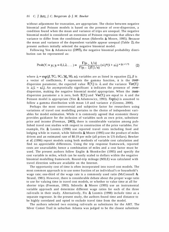
Following Yen & Adamowicz (1993), the negative binomial probability distri-bution can be represented as:

Prob(Y; = y;; yi = 0,1,2, . . . ) = I-@ + l’@)

r(yi + l)r(l/a)

(&)Y,(l + (.&) - (yt+ 119(2)

where Ri = exp(P, TCi, SC, Mi, SEi, ui), variables are as listed in equation (l), /3 isa vector of coefficients, I represents the gamma function, c( is the over-dispersion parameter, the expected value E(Y;) is 3,i and the variance Var(Yi)is ,$(l + HAi). An asymptotically significant CI indicates the presence of over-dispersion, making the negative binomial model appropriate. When the over-dispersion parameter a is zero, both E(Yi) and Var(Yi) are equal to li and thePoisson model is appropriate (Yen & Adamowicz, 1993). Exp(ui) is assumed tofollow a gamma distribution with mean 1.0 and variance 0 (Greene, 2000).

Perhaps the most controversial and subjective factor for researchers usingvariations of travel cost modelling pertains to the choice of independent vari-ables for model estimation. While it is commonly agreed that economic theoryprovides guidance for the inclusion of variables such as own price, substituteprice and income (Freeman, 1993), there is considerable variation among pub-lished travel cost studies with respect to construction of the price variables. Forexample, Fix & Loomis (1998) use reported travel costs including food andlodging while in transit, while Siderelis & Moore (1995) use the product of milesdriven and an estimated rate of $0.19 per mile (all prices in US dollars). Bowkeret ~2. (1996) report models using both methods of variable cost calculation andfind no appreciable differences. Using the trip response framework, reportedcosts are unavailable; hence a combination of miles and a cost factor must beused. The present authors follow Englin & Shonkwiler (1995) and specify thecost variable in miles, which can be easily scaled to dollars within the negativebinomial modelling framework. Round-trip mileage (MILE) was calculated withtravel direction software available on the Internet.

The opportunity cost of time is often incorporated into travel cost models. Themost common approach is to use some fraction of an individual’s or household’swage rate; one-third of the wage rate is a commonly used ratio (McConnell &Strand, 1981). However, there is considerable debate about the proper wage ratioto use for valuing time in travel cost models, or whether to value time at all forshorter trips (Freeman, 1993). Siderelis & Moore (1995) use an instrumentalvariable approach and determine different wage ratios for each of the threerail-trails in their study. Alternatively, Fix & Loomis (1998) include time as aseparate regressor. In the present study, the authors found time and distance tobe highly correlated and opted to exclude travel time from the model.

The authors selected two existing rail-trails as substitutes for the ART. TheSilver Comet Trail in suburban Atlanta was judged to be the closest substitute

A Contingent Trip Model for Estimating Rail-trail Demand 8 7

site for the large majority of the study’s sample; the remainder lived closer to arail-trail in suburban Augusta, Georgia. It was assumed that if an individualsought out information on rail-trails in general, information on the Silver Cometand Augusta rail-trail would be readily available. Round-trip substitute sitemileage (SUBMILE) was constructed for each zip code to substitute site combi-nation.

While many recreation demand studies, including Fix & Loomis (1998) andSiderelis & Moore (1995), do not find income to be a statistically significantvariable, the authors chose to include household income (HHINC) for theoreticalreasons. In particular, income imposes a budget constraint on consumption thatshould be accounted for in demand functions. In addition to income, Loomis &Walsh (1997) list a number of candidate socio-economic variables that may beincluded in travel cost demand models, including age, education, race, gender,occupation and others. Bayless et al. (1994) included a total of nine socio-economic variables in their TRM model. After dropping income because of thelack of statistical significance, Fix & Loomis (1998) included age as the onlysocio-economic demand shifter, while Siderelis & Moore (1995) use a variablereflecting the age composition of each visitor group. Both studies found mixedresults with age variables. Given these results, and no clear theoretical guidance,the present authors chose to include the age (AGE) of the respondents.

Siderelis & Moore (1995) use binary variables to differentiate users by bikingand walking activities. The authors follow this approach by using a dummyvariable (DBIKE) for respondents who biked on a regular basis. The authors alsoincluded binary variables to indicate previous experience with rail-trails(DPREV) and whether the individual lived in a rural county (DRURAL). Anumber of studies have found experience, either with a specific site or inreference to a given activity, to be significant in explaining recreation behaviour(Schreyer et al., 1984; Bowker & Leeworthy, 1998; Furuseth & Altman, 1991). Thepresent authors included the rural variable to account for possible differences intastes and preferences between rural and suburban residents. Moreover, giventhat the rail-trail would be situated in a rural area but the majority of users inthe sample are from surrounding suburban areas, the authors felt it importantto see if differences in tastes and preferences existed, as these could haveimportant policy ramifications.

Results

Table 2 lists summary statistics for a number of variables in the questionnairerelated to the empirical model. Mean annual household income for the samplewas about $64 400. This compares favourably to 1999 estimates of mean house-hold income in Georgia of $70 500 (Woods & Poole Economics, Inc., 1997) andmean household income of $60 200 for the 41 sample counties (1999 dollars, USCensus Bureau, provided by Survey Sampling, Inc.). Sample proportions forgender and race differed considerably from those reported in the 2000 census forGeorgia. Males represented 63% of the present sample, while males make upslightly over 49% of the state’s population. Similarly, non-whites comprised 17%of the sample, while making up about 35% of the state’s population. Averageage of the survey respondents was about 47 years, ranging from 18 to 87. Themean household size of respondents was about 2.6.

8 8 C. J. Betz, J. C. Bergstrom &J. M. Bowker

Regarding individual tastes and preferences, about 20% of the sample hadprevious experience with rail-trails. About 31% of the sample said they werefamiliar with the term ‘rail-trail’ before receiving the survey. Nearly 47%responded that they had previously used a more generic ‘greenway’ trail.Almost three-fourths of the respondents were occasional or frequent walkers,regardless of location. A much lower proportion, 23%, rode mountain bikes orroad bicycles either occasionally or often in the past year. Forty-one per cent ofthe sample expressed strong support, in a Likert-type question, for convertingabandoned railways to public use trails in their communities.

Table 2 also includes variables used for demand modelling. Respondentsanticipated, on average, taking fewer than two trips annually to the ART. Justunder 99% of respondents reported 12 or fewer trips per year, while no onereported 13 to 29 trips per year. Approximately 1% of the sample, four observa-tions, reported expecting to make from 30 to 50 trips. About 38% of respondentssaid they would take zero trips to the rail-trail. More than half of these (56%)said they might visit the ART, but would not make any trips specifically to doso. Time and cost constraints were the next most common reason for a zero-tripsresponse, about 26%. The mean distance of all survey respondents from therail-trail was about 52 miles one-way. Travel time to the rail-trail averaged about72 minutes one-way with a high of more than two hours. Average distance toeither substitute site was 42 miles one-way.

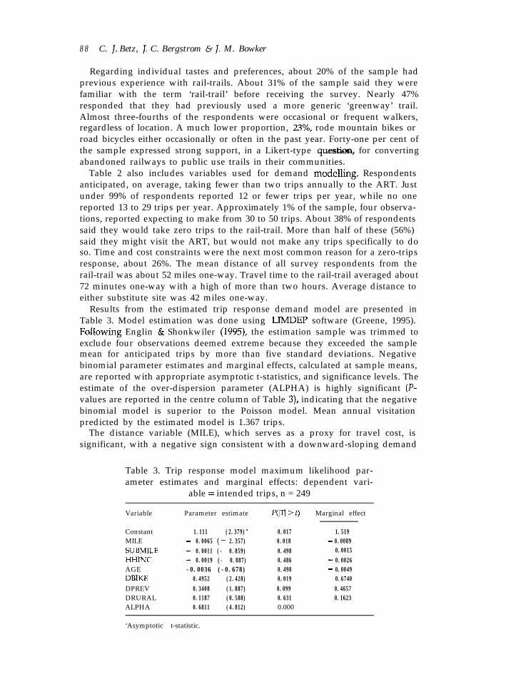
Results from the estimated trip response demand model are presented inTable 3. Model estimation was done using LIMDEP software (Greene, 1995).FoILowing Englin & Shonkwiler (1995), the estimation sample was trimmed toexclude four observations deemed extreme because they exceeded the samplemean for anticipated trips by more than five standard deviations. Negativebinomial parameter estimates and marginal effects, calculated at sample means,are reported with appropriate asymptotic t-statistics, and significance levels. Theestimate of the over-dispersion parameter (ALPHA) is highly significant (P-values are reported in the centre column of Table 3), indicating that the negativebinomial model is superior to the Poisson model. Mean annual visitationpredicted by the estimated model is 1.367 trips.

The distance variable (MILE), which serves as a proxy for travel cost, issignificant, with a negative sign consistent with a downward-sloping demand

Table 3. Trip response model maximum likelihood par-ameter estimates and marginal effects: dependent vari-

able = intended trips, n = 249

Variable Parameter estimate w ’ f) Marginal effect

ConstantMILESUBMILEHJc-IINCAGEDBIKEDPREVDRURALALPHA

1.111 (2.379)" 0.017- 0.0065 (- 2.357) 0.018- 0.0011 (- 0.859) 0.498- 0.0019 (- 0.887) 0.486-0.0036 (-0.678) 0.498

0.4952 (2.428) 0.0190.3408 (1.887) 0.0990.1187 (0.588) 0.6310.6811 (4.812) 0.000

1.519- 0.0089- 0.0015- 0.0026- 0.0049

0.67400.46570.1623

‘Asymptotic t-statistic.

A Contingent Trip Model for Estimating Rail-trail Demand 8 9

curve. Counter to economic theory, the household income variable, HHINC, hada negative although insignificant coefficient. One possible reason is that peopleof similar incomes choose similar recreation pursuits. However, given the rangeof incomes in the study, one might argue that people of all incomes partake ofrail-trail recreation. Multicollinearity is another possible reason, which wouldcause inflated coefficient variance; however, correlation coefficients betweenincome and other explanatory variables show no apparent problems. Bowker &Leeworthy (1998) note that insignificant income coefficients are not uncommonin recreation demand studies. Both Siderelis & Moore (1995) and Fix & Loomis(1998) exclude income from their reported demand models.

The substitution variable, SUBMILE, was also insignificant. A number offactors could account for this. While the authors chose two existing rail-trail sitesas likely substitutes for the ART, it is possible that individuals would substitutealternative locations offering similar activity venues, like state and local parks,or that individuals would substitute different activities altogether. Fix & Loomis(1997) were more successful in identifying substitute variables. This is probablyrelated to the fact that the demand function they modelled was for a speciallocation (Moab), with a very specialized activity (mountain biking). Altema-tively, Siderelis & Moore (1995) could not find an adequate substitute for any oftheir rail-trail sites.

The binary variable identifying bikers (DBIKE = 1) was significant with apositive sign. This indicates that when other factors are equal, bikers woulddemand more trips than non-bikers. The authors obtain a similar result forindividuals who claim to have previously used a rail-trail (DPREV = 1). Thisresult corroborates previous recreation research suggesting that experienceaffects recreation choices and behaviour.

A final variable in the model was DRURAL, indicating whether the individuallived in a rural area. The coefficient for this variable was positive, suggestingthat rural dwellers would be more likely to use the ART. However, the resultwas not statistically significant. The lack of a significant difference between ruraland non-rural suggests that development of a rail-trail in a rural area would notnecessarily lead to excessive use by outsiders.

Economic and Use Measures

Two important economic policy measures can be derived from the estimateddemand model: price elasticity of demand (0 and consumer surplus (CS). Priceelasticity is a unitless measure of demand response to changes in a good orservice’s price. It is defined as the percentage change in quantity demandeddivided by the percentage change in the price. Price elasticity is negative becauseof the inverse relationship between price and quantity. A unitary elasticityimplies that price and quantity change in the same proportion. Price elasticitytypically encountered in recreation demand studies ranges from about - 0.2 to- 2.0 (Loomis & Walsh, 1997).

Within the negative binomial model’s semi-log form, price elasticity is derivedas [ = & X TC, where & is the estimated coefficient on the travel cost variableand TC is travel cost. As distance or travel cost increases so does the estimatedelasticity. At the sample mean for roundtrip distance of 104.6 miles, [ = - 0.68.Elasticities calculated from the Siderelis & Moore (1995) study, using thenegative binomial estimates, range from - 0.207 for the suburban Lafayette

9 0 C. J. Betz, J. C. Bergstrom &J. M. Bowker

Morgana Trail in Oakland, California, to - 0.235 for the St Mark’s Trail innorthern Florida, to - 0.430 for the Heritage Trail in rural Iowa.

While the present authors’ results can be termed moderately inelastic, they aremore elastic, and hence price sensitive, than those of Siderelis & Moore (1995).The differences could be due to a number of reasons, the most basic being thatthere are inherent differences in surveyed populations, with the authors’ resultssuggesting that general public demand for rail-trail use is more price sensitivethan the on-site user population examined by Siderelis & Moore (1995). Cer-tainly, the authors’ sample of potential users would not have developed anyaffinity or place attachment effects that might make their demand more priceinelastic. Another explanation for the elasticity differences is that demand andsupply relationships may have changed somewhat since Siderelis & Moore’s(1995) data were collected in 1991. Siderelis & Moore (1995) state that suitablesubstitute sites were not readily identifiable at the time of their work. Also, thehigher proportion of local users in their study, coupled with the fact that theformula for elasticity in count models forces elasticity to increase as distance(cost increases), could be a factor. Finally, a basic methodological differencestems from the present authors’ use of the trip-response method versus Siderelis& Moore (1995) using on-site surveying and standard travel cost models.

A practical implication of the inelastic price elasticity pertains to the im-plementation of access or parking fees that could be used to supplement publicfunding for trail maintenance. For example, using a per-mile cost of 12 cents,’sample average travel cost is $12.56 and [ = - 0.681. Price would have to rise toapproximately $18.46 before the unitary portion of the demand curve wasreached, implying that entry or parking fees of up to $5.90 would depressvisitation by a lesser percentage than the increase in price and consequently leadto increases in revenue. This is conditioned by the assumption that usersresponded similarly to the on-site fees as to any other increase in travel cost.

The other important measure gleaned from demand estimation is CS or neteconomic value. It expresses a non-observable measure of utility in terms ofdollars and is interpreted as willingness to pay (WTP) for access to the site overand above the necessary travel cost (Bergstrom, 1990; Siderelis & Moore, 1995).Typically, for recreation applications, use is measured in visits, trips or rec-reation days. For day use sites, these measures are equal. Hence, for economicvaluation it is convenient to derive consumer surplus on a per-trip basis. Usingthe negative binomial specification, per-trip consumer surplus is calculated asCS = - l/& (Creel & Loomis, 1990). Unlike the calculated price elasticity, CSper trip varies with assumed per-mile travel cost. Using 12 cents per mile,per-trip consumer surplus for access to the ART is $18.46. Following Siderelis &Moore (1995), using 19 cents per mile, CS per trip is $29.23. The latter estimatefalls within the range of estimated surpluses ($9.56, $30.18, $49.78) for the threerail-trails (Lafayette-Morgana, Heritage, St Mark’s) in their study.

CS estimates can be of use to regional, state and local planners in estimatingaggregate benefits necessary for a cost-benefit analysis of the ART. For example,aggregate annual net economic value can be estimated by combining consumersurplus per trip ($18.46) with annual visitation. Visitation can be approximatedby combining average predicted annual trips (1.367), the product of the numberof households in the 75-mile study radius (780 697) and the percentage ofhouseholds responding to the survey (0.39). This yields an estimated 416 213household visits with aggregate annual benefits totalling over $7.5 million.

A Contingent Trip Model for Estimating Rail-trail Demand 91

Previous studies have shown evidence that WTP stated in contingent valu-ation surveys may over-estimate actual WTP, including applications to green-way projects, of which rail-trails are a special case (Lindsey & Knaap, 1999). Theobserved differences between stated WTP and actual WTP observed in previousstudies are often relatively small, suggesting that in well-designed contingentvaluation studies, stated WTP provides a reasonable approximation of actualWTP (Mitchell & Carson, 1989; Boyle & Bergstrom, 1999). To the presentauthors’ knowledge, previous validation studies have not been conducted tocompare stated trip responses to actual trip responses. If the results of validationstudies comparing stated and actual WTP carry over to trip response studies, itis possible that the authors’ estimates of stated mean trips and WTP (CS) perperson associated with the ART derived from the trip response model over-estimate actual mean trips and WTP per person. More research is needed to testand confirm the extent to which stated trip responses and actual trip responsesmay differ.

Because of the possibility that stated trip responses may over-estimate actualtrip responses, the present estimate of aggregate annual benefits includes severalconservative use assumptions. First, the authors assumed that neither thenon-respondents nor those beyond the imposed 75-mile radius would take tripsto the ART. Secondly, the study is focused at the household level, and hencemay under-count total visits, which could include additional household mem-bers. Thirdly, the estimate is based on the assumption that local demand wouldnot be further stimulated by the existence of the site. In addition, the wordingof the trip response question does not explicitly mention fitness as a reason fortaking rail-trail trips, because the authors assumed that fitness was subsumed inrecreation. However, as suggested by one of the reviewers, if some respondentsexcluded fitness trips because of the particular wording of the trip responsequestion, the expected effect would be to under-estimate use. This effect, ifindeed present in the trip response model results, would also help to offset apotential tendency for respondents to over-estimate stated trips as compared toactual trips.

A final potential source of error pertains to sample versus population propor-tions. The sample contained higher proportions of whites and males than recentcensus figures for the area. Also, a disproportionately high proportion ofrespondents, 56%, reported having at least four years of college. These propor-tions are not unlike those reported by Furuseth & Altman (1991). Because it hasbeen documented that white males are more likely to engage in trail-basedactivities than other race/gender combinations (Bowker et al., 1999), the authors’estimate of 1.367 visits per household, even in the absence of hypothetical bias,would not be appropriate for extrapolation across all area households. Rather, asegmented procedure, albeit ad hoc, as the authors followed with respondentsand non-respondents, should be used. A related alternative for future researchwould be to explore the development of two-stage procedures combiningsample and non-sample information to first predict whether a household wouldbe a potential market entrant, and if so, how many trips they would take. Suchmodels have been suggested for use in recreation demand modelling to mitigatethe problem of non-response bias.

These caveats notwithstanding, the authors’ visitation estimate appears to bein line with a number of previous studies. For example, Hunter & Huang (1995)report use estimates from a number of studies of multipurpose trails ranging

9 2 C. J. Betz, J. C. Bergstrom & J. M. Bowker

from over 2000 per day in metropolitan New York to 200 per day outsideProvidence. On the same trails studied by Siderelis & Moore (1995), Moore et al.(1994) report estimated annual user densities ranging from 52 632 per mile forthe urban Lafayette-Morgana Trail to 5192 for the Heritage Trail in rural Iowaand 10 625 for the St Mark’s Trail proximal to a major university in Florida. Ina study of the North Central Rail Trail outside Baltimore, PFK Consulting (1994)reported an annual visitation estimate of 457540 on the 20-mile length of thetrail. The present authors’ estimate is also relatively close to Lindsey’s (1999)visitation estimates of 456 600 and 379 500 for two sections of the Monon Trailin Indianapolis.

Summary and Conclusions

This study examined the demand for and value of access to a proposed rail-trailthat would result from conversion of a 23-mile-long stretch of abandonedrailway corridor in north-east Georgia to a public use trail that prohibitsmotorized vehicles. Rail-trails have been touted for providing much-neededclose-to-home recreation resources that support popular activities like walking,bicycling, in-line skating and wildlife viewing. In many cases, they are alsoconsidered important regional tourism attractions that bring in significantamounts of visitor spending to local economies.

The authors used a contingent trip approach, a stated preference variant of thetravel cost method, to estimate net benefits or consumer surplus values associ-ated with rail-trail trips. This approach provides a cost-effective alternative toon-site sampling and more traditional travel cost modelling in a number ofways. First, it allows planners to obtain demand and value information about apotential site or management alternative at a given site for which comparablestudies do not exist. Secondly, it incorporates information from non-users intothe formulation of the demand model, thus circumventing problems of zero-truncation and endogenous stratification (Siderelis & Moore, 1995).

Although the CTM or TRM has been applied in past studies, more researchusing this type of hybrid model is recommended to verify its utility and validity.The authors’ findings of per-trip consumer surplus and price elasticity suggestthat the per-trip economic measures are reasonable. These results notwithstand-ing, there are a number of limitations and caveats that must be mentioned. First,the CTM is still subject to criticism associated with its intended behaviourunderpinning. Nevertheless, techniques based on hypothetical or intended be-haviour are prevalent in marketing research conducted in the private sector.However, there exists an important need to develop comparison experimentswhereby the aggregate use estimates developed from CTM models can bevalidated against actual counts. Secondly, with a response rate of about 40%, thepossibility of non-response bias is a concern. In this study, income levels ofsample respondents were reasonably close to census figures for the region.However, the minorities are under-represented, while males and college gradu-ates are over-represented.

The most salient policy implication from this study is the basic fact that adiscernible demand for the proposed ART would exist with considerable econ-omic value. Identification of tourism markets is critical because they representthe demand side of the industry, without which there would be no need fortourism suppliers or producers. It is expected that the ART’s potential market

A Contingent Trip Model for Estimating Rail-trail Demand 9 3

would consist primarily of regional day users. There was some evidence,however, of potential users living beyond a one- to two-hour drive, as far awayas 200 miles one-way. This has important implications with respect to tourismdevelopment objectives, as the ART would possess attributes and characteristicssimilar to other rail-trails in the USA that have proven to be successful tourismattractions.

The estimates of aggregate value would prove useful to a cost-benefit analysisassessing the economic feasibility of converting the rail corridor to a public usetrail. If costs exceeded the most conservative value estimate, decision makerswould need to weigh the credibility of the other estimates in the process. Theauthors did not consider the cost side of the equation, but an accounting ofacquisition, development, maintenance, economic and other costs to convert thecorridor into the ART would be fairly straightforward.

Model findings might also have implications for the marketing and manage-ment of the proposed ART. One is an improved understanding of the potentialusers. For example, none of the basic socio-economic variables was statisticallysignificant, indicating that among respondents, no specific demographic segmentwould more likely to frequent the rail-trail. However, whites, males and collegegraduates were over-represented in the sample, suggesting that results from asingle-stage model should be interpreted cautiously. More research is neededbefore conclusions can be drawn about the type of individuals that wouldcharacterize the market. The cost variables show that users do respond to priceat less than unitary elasticity. This is important information if user fees wereever considered. Not surprisingly, the more avid potential users would bebicyclists and those with previous rail-trail experience. This knowledge of userscould prove useful toward building constituent groups and public support.

More economic research on the demand for and valuation of rail-trails iswarranted as these dormant resources are considered for conversion to viablerecreation destinations. As a relatively new and increasingly popular type ofrecreation resource, additional, credible economic information about the benefitsand costs of these resources is needed. Very little previous work addressingeconomic values of rail-trails has been accomplished. More is needed forcomparative purposes. More research has evaluated the more generic ‘green-ways’, especially in urban areas. While similar in many respects, there aredistinctive differences between rail-trails and the more general greenways,including types of surfaces, lengths, grades, environments and settings. Allrail-trails are also considered ‘greenways’, but the reverse is not true. Researchinto user preferences for the various attributes of greenways and rail-trailswould help improve understanding of economic value and demand. Of particu-lar interest would be knowing more about the differences in attributes (beyondjust their location) between greenways and rail-trails that are recognized astourist attractions and those that are not. More information on the characteristicsof individuals who demand rail-trail trips, perhaps through some kind ofclustering technique that examined demographics with attitudes and desiredattributes, would also prove helpful in improving rail-trail demand models.

Acknowledgements

This research benefited from the helpful comments of Dr Greg Lindsey and thejournal’s reviewers. The authors are also grateful for the support of the Georgia

9 4 C. J. Betz, J. C. Bergstrom i3 J. M. Bowker

Agricultural Experiment Station and Southern Research Station of the USDepartment of Agriculture Forest Service. Responsibility for both the viewsexpressed in this paper and any remaining errors rests with the authors.

Notes

1. As a matter of protocol, many contingent valuation questionnaires include a statement remind-ing respondents to consider their budget constraint when answering willingness-to-pay ques-tions. We did not include such a statement in our questionnaire. We assume that whenanswering the trip response question, respondents to our survey considered their budgetconstraints as well as substitutes. An interesting future experiment would be to test whether ornot budget constraint reminders result in statistically significant changes in mean responses totrip response questions.

2. Federal guidelines recommend using the most current figures from the U.S. Department ofTransportation or American Automobile Association (AAA) on the average per-mile cost ofoperating automobiles (Loomis & Walsh, 1997). AAA’s 1998 edition of Your Driving Costs citesan average operating cost of $0.12 per mile for an 8-cylinder, I-door passenger sedan and thesame cost for a 6-cylinder, 2-door sport utility vehicle.

References

Athens Daily News (1999) Athens-to-Madison rails-to-trails project could pay, Editorial, 29 June.Bayless, D.S., Bergstrom, J.C., Messonnier, M.L. & Cordell, H.K. (1994) Assessing the demand for

designated wildlife viewing sites, journal of Hospitality and Leisure Marketing, 2(3), pp. 75-93.Bemisderfer, T.R. (1995) Using abandoned railroad rights-of-way in rural landscapes as nature

conservation and linear recreation areas, unpublished master’s thesis (Athens, GA, Department ofLandscape Architecture, University of Georgia).

Bergstrom, J.C. (1990) Concepts and measures of the economic value of environmental quality: areview, Journal of Environmental Management, 31, pp. 215-228.

Bowker, J.M. & Leeworthy, V.R. (1998) Accounting for ethnicity in recreation demand: a flexiblecount data approach, Journal of Leisure Research, 30(l), pp. 64-78.

Bowker, J.M., English, D.B.K. & Donovan, J.A. (1996) Toward a value for guided rafting on Southernrivers, Journal of Agricultural and Applied Economics, 28(2), pp. 423432.

Bowker, J.M., English, D.B.K. & Cordell, H.K. (1999) Projections of outdoor recreation participationto 2050, in: H. K. Cordell (Ed) Outdoor Recreation in American Life: A National Assessment of Supplyand Demand Trends (Champaign, IL, Sagamore Publishing).

Boxall, P.C., McFarlane, B.L. & Gartrell, M. (1996) An aggregate travel cost approach to valuing forestrecreation at managed sites, Forest Chronicles, 72, pp. 615-621.

Boyle, K.J. & Bergstrom, J.C. (1999) Doubt, doubts, and doubters: the genesis of a new researchagenda?, in: I. J. Bateman & K. G. Willis (Eds) Valuing Environmental Preferences: Theory and Practiceof the Contingent Valuation Method in the US, EU and Developing Countries (New York, OxfordUniversity Press).

Carr, G. (2000) Rails to trails keeps the faith, Flagpole Magazine, 26 January.Carr, J.B., Delhomme, K.A. & Johnson, L.S. (1998) Assessing Community Impacts from Greenways:

Recommendations for Idenfr$jng, Measuring, and Estimating the Benefits and Costs of Corridors (Talla-hassee, FL, Center for International Public Management, Inc. & Florida Department of Environ-mental Protection, Office of Greenways and Trails).

Creel, M.D. & Loomis, J.B. (1990) Theoretical and empirical advantages of truncated count dataestimators for analysis of deer hunting in California, American Journal of Agricultural Economics, 72,pp. 434441.

Dawson, K.J. (1995) A comprehensive conservation strategy for Georgia’s greenways, landscape andUrban Planning, 33, pp. 2743.

Dillman, D.A. (1978) Mail and Telephone Surveys: The Total Design Method (New York, Wiley).Englin, J. & Shonkwiler, J.S. (1995) Estimating social welfare using count data models: an application

to long-run recreation demand under conditions of endogenous stratification, Reviezc of Economicsand Statistics, 77, 104-112.

English, D.B.K. & Bowker, J.M. (1996) Sensitivity of whitewater rafting consumer’s surplus topecuniary travel cost specifications, Journal of Environmental Management, 47, pp. 79-91.

A Contingent Trip Model for Estimating Rail-trail Demand 9 5

Fix, I’. & Loomis, J.B. (1997) The economic benefits of mountain biking at one of its Meccas: anapplication of the travel cost method to mountain biking in Moab, Utah, journal of Leisure Research,29(3), pp. 342-352.

Fix, P. & Loomis, J.B. (1998) Comparing the economic value of mountain biking estimated usingrevealed and stated preference, lournal of Environmental Planning and Management, 41(2), pp. 227-2 3 6 .

Forsberg, M. (1994) Rails-to-trails, Nebraskaland, June, pp. 44-55.Freeman III, A.M. (1993) The Measurement of Environmental and Resource Values (Washington, DC,

Resources for the Future).Furuseth, O.J. & Altman, R.E. (1991) Who’s on the greenway: socioeconomic, demographic, and

locational characteristics of greenway users, Environmental Management, 15(3), pp. 329-336.Greene, W.H. (1995) LIMDEP, Version 7.0 (Plainview, NY, Econometric Software, Inc.).Greene, W.H. (2000) Econometric Analysis, 4th edition (EngIewood Cliffs, NJ, Prentice-Hall).Hof, J. (1993) Coactive Forest Management (New York, Academic Press).Hunter, W.W. & Huang, H.F. (1995) User counts on bicycle lanes and multiuse trails in the United

States, Transportation Research Record, 1502, pp. 45-57.Layman, R.C., Boyce, J.R. & Criddle, K. (1996) Economic valuation of the Chinook salmon sport

fishery of the Gulkana River, Alaska, under current and alternate management plans, LandEconomics, 72(l), pp. 113-128.

Leeworthy, V.R. & Bowker, J.M. (1997) Nonmarket Economic User Values of the Florida Keys/Key West,National Oceanic and Atmospheric Administration, Strategic Environmental Assessments Division(http://www-orca.nos.noaa.gov/projects/eco~lkeys/ecollkeys.h~l).

Lindsey, G. (1999) Use of urban greenways: insights from Indianapolis, Landscape and Urban Planning,45, pp. 145157.

Lindsey, G. & Knaap, G. (1999) Willingness to pay for greenway projects, Journal of the AmericanPlanning Association, 65(3), pp. 297-313.

Loomis, J.B. & Walsh, R.G. (1997) Recreation Economic Decisions: Comparing Benefits and Costs, 2ndedition (State College, PA, Venture Publishing).

McConnell, K.E. & Strand, I. (1981) Measuring the cost of time in recreation demand analysis:applications to sport fishing, American Journal of Agricultural Economics, 61, pp. 153-156.

Mitchell, R.C. & Carson, R.T. (1989) Using Surveys to Value Public Goods: The Contingent ValuationMethod (Washington, DC, Resources for the Future).

Moore, R.L., Graefe, A.R. & Gitelson, R.J. (1994) The economic impact of rail-trails, Journal of Park andRecreation Administration, 12(2), pp. 63-72.

Morris, H. (2000) [Research Director, Rails-to-trails Conservancy, Washington, DC] Personal com-munication.

National Bicycle and Pedestrian Clearinghouse (1995) The Economic and Social Benefits of Of-roadBicycle and Pedestrian Facilities, National Bicycle and Pedestrian Clearinghouse Technical Brief,Technical Assistance Series, Number 2 (Washington, DC, US Department of Transportation).

National Park Service (1995) Economic Impacts of Protecting Rivers, Trails and Greetzzuay Corridors: AResource Book (Washington, DC, Rivers, Trails and Conservation Assistance Division).

PFK Consulting (1994) Analysis of Economic Impacts of the Northern Central Rail Trail, prepared forMaryland Greenways Commission (Annapolis, MD, Maryland Department of Natural Resources).

President’s Commission on Americans Outdoors (PCAO) (1986) Report and Recommendations to thePresident of the United States (Washington, DC, US Government Printing Office).

Rails-to-trails Conservancy (RTC) (2001) (www.railtrails.org).Randall, A. (1994) A difficulty with the travel cost method, Land Economics, 70(l), pp. 8896.Ribaudo, M.O. & Epp, D.J. (1984) The importance of sample discrimination in using the travel cost

method to estimate the benefits of improved water quality, land Economics, 60(4), pp. 397403.Schreyer, R., Lime, D.W. & Williams, D.R. (1984) Characterizing the influence of past experience on

recreation behavior, journal of Leisure Research, 16(l), pp. 34-50.Siderelis, C. & Moore, R.L. (1995) Outdoor recreation net benefits of rail-trails, Journal of Leisure

Research, 27(4), pp. 344359.Smith, D.S. (1993) An overview of greenways: their history, ecological context, and specific functions,

in: D. S. Smith & P. C. Hellmund (Eds) Ecology of Greenzoays: Design and Function of LinearConservation Areas (Minneapolis, MN, University of Minnesota Press).

Smith, V.K. (1988) Selection and recreation demand, American Journal of Agricultural Economics, 70,pp. 29-36.

Teasley, R.J., Bergstrom, J.C. & Cordell, H.K. (1994) Estimating revenue-capture potential associatedwith public area recreation, Iournal of Agricultural and Resource Economics, 19(l), pp. 89-101.

9 6 C. J. Betz, J. C. Bergstrom & J M. Bowker

US Census Bureau (1998) Educational Attainment of Persons 15 Years Old and Over, by Age, Sex, Race,and Hispanic Origin, March 1998 (wwwcensusgov).

Vaughn, W.J. & Russell, C.S. (1982) Valuing a fishing day: an application of a systematic varyingparameter model, Land Economics, 58, pp. 450463.

Woods & Poole Economics, Inc. (1997) The Complete Economic and Demographic Data Source (Washing-ton, DC, Woods & Poole Economics, Inc.).

Yen, S.T. & Adamowicz, W.L. (1993) Statistical properties of welfare measures from count datamodels of recreation demand, Review of Agricultural Economics, 15(2), pp. 203-215.

Zawacki, W.T., Marsinko, A. & Bowker, J.M. (2000) A travel cost analysis of nonconsumptivewildlife-associated recreation in the United States, Forest Science, 46(4), pp. 496-506.