A consistent bootstrap procedure for the maximum score ...emilio/maxScoreEstimator.pdfBootstrap methods avoid the problem of estimating nuisance parameters and are generally reliable

A consistent bootstrap procedure for the maximum

score estimator

Rohit Kumar Patra, Emilio Seijo, and Bodhisattva Sen∗†

Department of Statistics, Columbia University

September 9, 2015

Abstract

In this paper we propose a new model-based smoothed bootstrap procedure

for making inference on the maximum score estimator of Manski (1975, 1985)

and prove its consistency. We provide a set of sufficient conditions for the

consistency of any bootstrap procedure in this problem. We compare the finite

sample performance of different bootstrap procedures through simulations stud-

ies. The results indicate that our proposed smoothed bootstrap outperforms

other bootstrap schemes, including the m-out-of-n bootstrap. Additionally, we

prove a convergence theorem for triangular arrays of random variables arising

from binary choice models, which may be of independent interest.

JEL classification: C14; C25

Keywords: Binary choice model, cube-root asymptotics, (in)-consistency of the

bootstrap, latent variable model, smoothed bootstrap.

∗Corresponding author. Tel.: +1 212 851 2149; fax: +1 212 851 2164. E-mail address:[email protected].†Research partially supported by NSF grant DMS-1150435 (CAREER)

1

1 Introduction

Consider a (latent-variable) binary response model of the form

Y = 1β>0 X+U≥0,

where 1 is the indicator function, X is an Rd-valued continuous random vector of

explanatory variables, U is an unobserved random variable and β0 ∈ Rd is an unknown

vector with |β0| = 1 (| · | denotes the Euclidean norm in Rd). The parameter of

interest is β0. If the conditional distribution of U given X is known up to a finite

set of parameters, maximum likelihood techniques can be used for estimation, among

other methods; see, e.g., McFadden (1974). The parametric assumption on U may be

relaxed in several ways. For instance, if U and X are independent or if the distribution

of U depends on X only through the index β>0 X, the semiparametric estimators of

Han (1987), Horowitz and Hardle (1996), Powell et al. (1989), and Sherman (1993)

can be used; also see Cosslett (1983). The maximum score estimator considered by

Manski (1975) permits the distribution of U to depend on X in an unknown and very

general way (heteroscedasticity of unknown form). The model replaced parametric

assumptions on the error disturbance U with a conditional median restriction, i.e.,

med (U |X) = 0, where med (U |X) represents the conditional median of U given X.

Given n observations (X1, Y1), . . . , (Xn, Yn) from such a model, Manski (1975) defined

a maximum score estimator as any maximizer of the objective function

n∑i=1

(Yi −

1

2

)1β>Xi≥0

over the unit sphere in Rd.

The asymptotics for the maximum score estimator are well-known. Under some

regularity conditions, the estimator was shown to be strongly consistent in Manski

2

(1985) and its asymptotic distribution was derived in Kim and Pollard (1990) (also

see Cavanagh (1987)). Even though the maximum score estimator is the most general

estimator available for the binary response model considered here, the complicated

nature of its limit law (which depends, among other parameters, on the conditional

distribution of U given X for values of X on the hyperplane x ∈ Rd : β>0 x = 0)

and the fact that it exhibits nonstandard asymptotics (cube-root rate of convergence)

have made it difficult to do inference for the estimator under complete generality.

As an alternative, Horowitz (1992) proposed the smoothed maximum score esti-

mator. Although this estimator is asymptotically normally distributed under certain

assumptions (after proper centering and scaling) and the classical bootstrap can be

used for inference (see Horowitz (2002); also see de Jong and Woutersen (2011) for

extensions to certain dependence structures), it has a number of drawbacks: it re-

quires stronger assumptions on the model for the asymptotic results to hold, the

smoothing of the score function induces bias which can be problematic to deal with,

and the plug-in methods (see Horowitz (1992, 2002)) used to correct for this bias are

not effective when the model is heteroscedastic or multimodal (see Kotlyarova and

Zinde-Walsh (2009)).

This motivates us to study the maximum score estimator and investigate the per-

formance of bootstrap — a natural alternative for inference in such nonstandard prob-

lems. Bootstrap methods avoid the problem of estimating nuisance parameters and

are generally reliable in problems with n−1/2 convergence rate and Gaussian limiting

distributions; see Bickel and Freedman (1981), Singh (1981), Shao and Tu (1995) and

its references. Unfortunately, the classical bootstrap (drawing n observations with

replacement from the original data) is inconsistent for the maximum score estimator

as shown in Abrevaya and Huang (2005). In fact, the classical bootstrap can behave

quite erratically in cube-root convergence problems. For instance, it was shown in

Sen et al. (2010) that for the Grenander estimator (the nonparametric maximum

3

likelihood estimator of a non-increasing density on [0,∞)), a prototypical example

of cube-root asymptotics, the bootstrap estimator is not only inconsistent but has

no weak limit in probability. This stronger result should also hold for the maximum

score estimator. These findings contradict some of the results of Abrevaya and Huang

(2005) (especially Theorem 4 and the conclusions of Section 4 of that paper) where

it is claimed that for some single-parameter estimators a simple method for inference

based on the classical bootstrap can be developed in spite of its inconsistency.

Thus, in order to apply the bootstrap to this problem some modifications of the

classical approach are required. Two variants of the classical bootstrap that can be

applied in this situation are the so-called m-out-of-n bootstrap and subsampling. The

performance of subsampling for inference on the maximum score estimator has been

studied in Delgado et al. (2001). The consistency of the m-out-of-n bootstrap can

be deduced from the results in Lee and Pun (2006). Despite their simplicity, the

reliability of both methods depends crucially on the size of the subsample (the m

in the m-out-of-n bootstrap and the block size in subsampling) and a proper choice

of this tuning parameter is difficult; see Section 4 of Lee and Pun (2006) for a brief

discussion on this. Thus, it would be desirable to have other alternatives — more

automated and consistent bootstrap procedures — for inference in the general setting

of the binary choice model of Manski.

In this paper we propose a model-based smoothed bootstrap procedure (i.e., a

method that uses the model setup and assumptions explicitly to construct the boot-

strap scheme; see Section 3.1 for the details) that provides an alternative to subsam-

pling and the m-out-of-n bootstrap. We prove that the procedure is consistent for

the maximum score estimator. In doing so, we state and prove a general convergence

theorem for triangular arrays of random variables coming from binary choice models

that can be used to verify the consistency of any bootstrap scheme in this setup.

4

We derive our results in greater generality1 than most authors by assuming that β0

belongs to the unit sphere in Rd as opposed to fixing its first co-ordinate to be 1 (as

in Abrevaya and Huang (2005)). To make the final results more accessible we express

them in terms of integrals with respect to the Lebesgue measure as opposed to surface

measures, as in Kim and Pollard (1990). We run simulation experiments to compare

the finite sample performance of different bootstrap procedures. Our results indicate

that the proposed smoothed bootstrap method (see Section 3.1) outperforms all the

others. Even though the proposed bootstrap scheme involves the choice of tuning

parameters, they are easy to tune — smoothing bandwidths that fit the data well are

to be preferred.

To the best of our knowledge, this paper is the first attempt to understand the be-

havior of model-based bootstrap procedures under the very general heteroscedasticity

assumptions for the maximum score estimator.

Our exposition is organized as follows: In Section 2 we introduce the model and

our assumptions. In Section 3 we propose the smoothed bootstrap procedure for the

maximum score estimator and discuss its consistency. We study and compare the

finite sample performance of the different bootstrap schemes in Section 4 through

simulation experiments. In Section 5 we state a general convergence theorem for

triangular arrays of random variables coming from binary choice models (see Theorem

5.1) which is useful in proving the consistency of our proposed bootstrap scheme (given

in Section 6). Section 7 gives the proofs of the results in Section 5. Appendix A

contains some auxiliary results and some technical details omitted from the main

text. In Appendix B we provide a necessary and sufficient condition for the existence

of the latent variable structure in a binary choice model, that may be of independent

interest.

1We do not need to assume that the coefficient corresponding to a particular covariate is non-zero.

5

2 The model

We start by introducing some notation. For a signed Borel measure µ on some

metric space X and a Borel measurable function f : X→ R which is either integrable

or nonnegative we will use the notation µ(f) :=∫fdµ. If G is a class of such

functions on X we write ‖µ‖G := sup|µ(f)| : f ∈ G. We will also make use of

the sup-norm notation, i.e., for functions g : X → Rd, G : X → Rd×d we write

‖g‖X := sup|g(x)| : x ∈ X and ‖G‖X := sup‖G(x)‖2 : x ∈ X, where | · | stands for

the usual Euclidean norm and ‖ · ‖2 denotes the matrix L2-norm on the space Rd×d

of all d× d real matrices (see Meyer (2001), page 281). For a differentiable function

f : Rd → R we write ∇f(x) := ∂f/∂x for its gradient at x. We will regard the

elements of Euclidean spaces as column vectors. For two real numbers a and b, we

write a ∧ b := min(a, b) and a ∨ b := max(a, b).

Consider a Borel probability measure P on Rd+1, d ≥ 2, such that if (X,U) ∼

P then X takes values in a closed, convex region X ⊂ Rd with X 6= ∅ (here X

denotes the interior of the set X) and U is a real-valued random variable that satisfies

med (U |X) = 0 almost surely (a.s.), where med (·) represents the median. We only

observe (X, Y ) ∼ P where

Y := 1β>0 X+U≥0 (1)

for some β0 ∈ Sd−1 (Sd−1 is the unit sphere in Rd with respect to the Euclidean norm).

Throughout the paper we assume the following conditions on the distribution P:

(C1) X is a convex and compact subset of Rd.

(C2) Under P, X has a continuous distribution with a strictly positive and continu-

ously differentiable density p on X. We also assume that ∇p is integrable (with

respect to the Lebesgue measure) over X. Let F denote the distribution of X

under P, i.e., F (A) := P (X ∈ A), for A ⊂ Rd Borel.

6

(C3) Define

κ(x) := P (Y = 1|X = x) = P(β>0 X + U ≥ 0|X = x

). (2)

We assume that κ is continuously differentiable on X, the set x ∈ X :

∇κ(x)>β0 > 0 intersects the hyperplane x ∈ Rd : β>0 x = 0, and that∫|∇κ(x)|xx>p(x)dx is well-defined.

Given observations (X1, Y1), . . . , (Xn, Yn) from such a model, we wish to estimate

β0 ∈ Sd−1. A maximum score estimator of β0 is any element βn ∈ Sd−1 that satisfies:

βn := argmaxβ∈Sd−1

1

n

n∑i=1

(Yi −

1

2

)1β>Xi≥0

. (3)

Note that there may be many elements of Sd−1 that satisfy (3). We will focus on

measurable selections of maximum score estimators, i.e., we will assume that we can

compute the estimator in such a way that βn is measurable (this is justified in view

of the measurable selection theorem, see Chapter 8 of Aubin and Frankowska (2009)).

We make this assumption to avoid the use of outer probabilities.

Our assumptions (C1)–(C2) on P and the continuous differentiability of κ imply

that Γ(β), defined as

Γ(β) := P[(Y − 1

2

)1β>X≥0

](4)

is twice continuously differentiable in a neighborhood of β0 (see Lemma A.1). More-

over, condition (C3) implies that the Hessian matrix ∇2Γ(β0) is non-positive definite

on an open neighborhood U ⊂ Rd of β0; see Lemma A.1. Our regularity conditions

(C1)–(C3) are equivalent to those in Example 6.4 of Kim and Pollard (1990) and

imply those in Manski (1985). Hence, a consequence of Lemmas 2 and 3 in Man-

ski (1985) is that β0 is identifiable and is the unique maximizer of the process Γ(β)

where β ∈ Sd−1. Similarly, Theorem 1 in the same paper implies that if (βn)∞n=1 is

any sequence of maximum score estimators, we have βna.s.−→ β0.

7

3 Bootstrap and consistency

3.1 Smoothed bootstrap

In this sub-section we propose a smoothed bootstrap procedure for constructing con-

fidence regions for β0. Observe that Y given X = x follows a Bernoulli distribution

with probability of “success” κ(x), i.e., Y |X = x ∼ Bernoulli(κ(x)), where κ is defined

in (2). Our bootstrap procedure is model-based and it exploits the above relationship

between Y and X using a nonparametric estimator of κ. The smoothed bootstrap

procedure can be described as follows:

(i) Choose an appropriate nonparametric smoothing procedure (e.g., kernel density

estimation) to construct a density estimator pn of p using X1, . . . , Xn.

(ii) Use (X1, Y1, ), . . . , (Yn, Xn) to find a smooth estimator κn of κ (e.g., using kernel

regression).

(iii) Sample (X∗n,1, Y∗n,1), . . . , (X∗n,n, Y

∗n,n) i.i.d. Qn (conditional on the data), where

(X, Y ) ∼ Qn if and only if X ∼ pn and Y |X = x ∼ Bernoulli(κn(x)).

(iv) Let β∗n be any maximizer of

S∗n(β) :=1

n

n∑i=1

(Y ∗n,i −

1

2

)1β>X∗n,i≥0.

(v) Compute

βn = argmaxβ∈Sd−1

∫β>x≥0

κn(x)− 1

2

pn(x)dx. (5)

Let Gn be the distribution of the (normalized and centered) maximum score estimator,

i.e.,

∆n := n1/3(βn − β0) ∼ Gn. (6)

8

Kim and Pollard (1990) showed that, under conditions (C1)–(C3), ∆n converges in

distribution. Let G denote the distribution of this limit. Thus,

ρ(Gn,G)→ 0,

where ρ is the Prokhorov metric or any other metric metrizing weak convergence of

probability measures. Moreover, let Gn be the conditional distribution of

∆∗n := n1/3(β∗n − βn) (7)

given the data, i.e., for any Borel set A ⊂ Rd, Gn(A) = P(∆∗n ∈ A

∣∣σ ((Xn, Yn)∞n=1)).

We will approximate Gn by Gn, and use this to build confidence sets for β0. In

Section 3.2, we will show that the smoothed bootstrap scheme is weakly consistent,

i.e.,

ρ(Gn, Gn)P−→ 0.

It was shown in Abrevaya and Huang (2005) that the bootstrap procedure based on

sampling with replacement from the data (X1, Y1), . . . , (Xn, Yn) (the classical boot-

strap) is inconsistent.

Steps (i)—(v) deserve comments. We start with (i). It will be seen in Theorem 5.1

that the asymptotic distribution of ∆n depends on the behavior of F , the distribution

of X under P, around the hyperplane H := x ∈ Rd : β>0 x = 0. As the empirical

distribution is discrete, a smooth approximation to F might yield a better finite

sample approximation to the local behavior around H. Indeed our simulation studies

clearly illustrate this point (see Section 4). We can use any nonparametric density

estimation method to estimate p. In our simulation studies, we use the “product

kernel function” constructed from a product of d univariate kernel functions and

9

estimate p by

pn(x) =1

nhn,1 · · ·hn,d

n∑i=1

K

(x−Xi

hn

), for x ∈ Rd, (8)

where hn = (hn,1, . . . , hn,d), K(x−Xihn

):= k

(x1−Xi,1hn,1

)× . . . × k

(xd−Xi,dhn,d

), and k(·)

is the density function of a symmetric random variable with finite variance; see Ein-

mahl and Mason (2005) and the references therein for the consistency of kernel-type

function estimators.

As noted after (2), κ plays a central role in determining the joint distribution

of (X, Y ) and in the absence of any prior knowledge on the conditional distribution

function of Y given X we can estimate it nonparametrically using the Nadaraya-

Watson estimator

κn(x) =

∑ni=1 YiK((x−Xi)/hn)∑ni=1K((x−Xi)/hn)

, (9)

where hn ∈ Rd is the bandwidth vector and K : Rd → R is the product kernel. A huge

literature has been developed on the consistency of the Nadaraya-Watson estimator;

see e.g., Li and Racine (2011) and the references therein.

In (iii), we generate the bootstrap sample from the estimated joint distribution of

(X, Y ). Note that our approach is completely nonparametric and allows us to model

any kind of dependence between X and Y . The maximum score estimator from the

bootstrap sample is computed in (iv).

Our bootstrap procedure does not necessarily reflect the latent variable structure

in (1); see Appendix B for a detailed discussion of this and a lemma discussing a

necessary and sufficient condition for the existence of the latent variable structure.

Therefore, βn is not guaranteed to be the maximum score estimator for the sampling

distribution at the bootstrap stage. For the bootstrap scheme to be consistent we

need to change the centering of our bootstrap estimator from βn to βn, the maximum

score estimator obtained from the smoothed joint distribution of (X, Y ). This is done

10

in (v).

Remark 3.1 In the above smoothed bootstrap scheme we generate i.i.d. samples from

the joint distribution of (X, Y ) by first drawing X from its marginal distribution and

then generating Y from the conditional distribution of Y |X. A natural alternative

is to draw Y ∼ Bernoulli(π) first (where π := P(Y = 1)) and then to generate X

from the conditional distribution of X|Y . In this approach, we need to estimate the

conditional density of X given Y = 0 (fX|Y=0) and Y = 1 (fX|Y=1) and π. Note that

κ and the conditional densities are related as

κ(x) =πfX|Y=1(x)

(1− π)fX|Y=0(x) + πfX|Y=1(x). (10)

A natural estimator of π, πn, can be the relative frequency of Y = 1 in the observed

data. Further, fX|Y=0 and fX|Y=1 can be estimated using standard kernel density

estimation procedures after partitioning the data based on the values of Y .

Remark 3.2 Note that κn in the smoothed bootstrap procedure, as described in Sec-

tion 3.1, does not necessarily satisfy the inequality (β>n x)(κn(x) − 1/2) ≥ 0 for all

x ∈ X. Thus the smoothed bootstrap procedure does not strictly mimic the latent vari-

able structure in the model. However, it must be noted that the referred inequality

will be satisfied asymptotically for all x outside the hyperplanex ∈ Rd : β>0 x = 0

whenever βn and κn are consistent.

3.2 Consistency of smoothed bootstrap

In this sub-section we study the consistency of the smoothed bootstrap procedure

proposed in the previous sub-section. The classical bootstrap scheme is known to

be inconsistent for the maximum score estimator; see Abrevaya and Huang (2005).

The consistency of subsampling and the m-out-of-n bootstrap in this problem can be

11

deduced from the results in Delgado et al. (2001) and Lee and Pun (2006), respec-

tively. However, finite sample performance of both subsampling and the m-out-of-n

bootstrap depend crucially on the choice of the block size (m), and the choice of a

proper m is very difficult. Moreover, different choices of m lead to very different

results. In contrast, the tuning parameters involved in the model based smoothed

bootstrap procedure can be easily calibrated — smoothing bandwidths that fit the

given data well are to be preferred.

We recall the notation and definitions established in Section 2. We will denote

by Z = σ ((Xn, Yn)∞n=1) the σ-algebra generated by the sequence (Xn, Yn)∞n=1 with

(Xn, Yn)∞n=1

i.i.d.∼ P. Let Qn be the probability measure on Rd+1 such that (X, Y ) ∼ Qn

if and only if

X ∼ pn and Y |X = x ∼ Bernoulli(κn(x)),

where pn and κn are estimators of p and κ respectively, and may be defined as in (8)

and (9). We can regard the bootstrap samples as (X∗n,1, Y∗n,1), . . . , (X∗n,n, Y

∗n,n)

i.i.d.∼ Qn.

Recall that Gn denotes the distribution of n1/3(βn−β0) and ρ(Gn,G)→ 0. More-

over, Gn denotes the conditional distribution of n1/3(β∗n − βn), given the data, where

βn is defined in (5). Thus, a necessary and sufficient condition for the smoothed

bootstrap procedure to be weakly consistent is

ρ(Gn,G)P−→ 0. (11)

In the following theorem, we give sufficient conditions for the smoothed bootstrap

procedure proposed to be consistent.

Theorem 3.1 (Main Theorem) Consider the smoothed bootstrap scheme described

in Section 3.1 and assume that assumptions (C1)–(C3) hold. Furthermore, assume

that the following conditions hold:

12

(S1) The sequence (pn)∞n=1 of densities is such that pn is continously differentiable

on X, ∇pn is integrable (with respect to the Lebesgue measure) over X, and

‖pn − p‖X = oP(n−1/3).

(S2) κn converges to κ uniformly on compact subsets of X w.p. 1.

(S3) For any compact set X ⊂ X, ‖∇κn−∇κ‖X → 0 a.s. and ‖∇κn−∇κ‖X = OP(1).

Then, the smoothed bootstrap procedure is weakly consistent, i.e., the conditional dis-

tribution of ∆∗n, given (X1, Y1), . . . , (Xn, Yn), converges to G in probability (see (11)).

The proof of Theorem 3.1 is involved and is given in Section 6. The proof uses

results from Section 5 where we give a convergence theorem for the maximum score

estimator for triangular arrays of random variables arising from the binary choice

model.

Conditions (S1)–(S3) deserve comments. In the following we discuss the existence

of pn and κn satisfying conditions (S1)–(S3). If we use kernel density estimation

techniques to construct pn, then Theorem 1 and Corollary 1 of Einmahl and Mason

(2005) give very general conditions on the uniform in bandwidth consistency of kernel-

type function estimators. In particular, they imply that (S1) holds if p is sufficiently

smooth. According to Stone (1982) the optimal and achievable rate of convergence

for estimating p nonparametrically is n−r

2r+d if p is r times continuously differentiable

over X. For the Nadaraya-Watson estimator Theorem 2 and Corollary 2 of Einmahl

and Mason (2005) gives numerous results on the uniform convergence of κn which,

in particular, shows that (S2) holds. The first condition in (S3) on the uniform

convergence on compacts (in the interior of the support of X) of ∇κn holds for the

Nadaraya-Watson estimator defined in (9); see Blondin (2007). The second condition

in (S3) can also be shown to hold under appropriate conditions on the smoothing

bandwidth and kernel if p is strictly positive on X.

13

Remark 3.3 Recall the alternative data generating mechanism described in Remark 3.1.

Let κn now be the estimator based on (10), where we use plug-in kernel density estima-

tors of fX|Y=0 and fX|Y=1, and estimate π by the sample mean of Y . Then, Theorem

1 and Corollary 1 of Einmahl and Mason (2005) (note that p(x) is bounded away from

zero on X) can be used to show that pn and κn satisfy conditions (S1)–(S3). Hence,

by Theorem 3.1, this smoothed bootstrap approach can also be shown to be consistent.

4 Simulation experiments

In this section we illustrate the finite sample performance of our proposed smoothed

bootstrap, the classical bootstrap, and the m-out-of-n bootstrap through simula-

tion experiments. Let (X∗1 , Y ∗1 ), . . . , (X∗m, Y∗m) be m samples drawn randomly with

replacement from (X1, Y1), . . . , (Xn, Yn). The m-out-of-n bootstrap estimates Gn

(see (6)) by the distribution of m1/3(βm − βn), where

βm := argmaxβ∈Sd−1

1

m

m∑i=1

(Y ∗i −

1

2

)1β>X∗i ≥0

.

Lee and Pun (2006) prove that such a bootstrap procedure is weakly consistent for

the binary response model considered in this paper if m = o(n) and m → ∞, as

n→∞. However finite sample performance of m-out-of-n bootstrap relies heavily on

the choice of m, and a proper choice is difficult. Also, most data driven choices for

m are computationally very expensive. For a comprehensive overview of m-out-of-n

bootstrap methods and discussion on the choice of m see Bickel et al. (1997) and

Bickel and Sakov (2008).

In our simulation study we take (X,U) ∼ P, where P is a distribution on Rd+1

and fix β0 = 1√d(1, . . . , 1)>. For P to satisfy our model assumptions, we let

U |X ∼ N

(0,

1

(1 + |X|2)2

), X ∼ Uniform([−1, 1]d), and Y = 1β>0 X+U≥0.

14

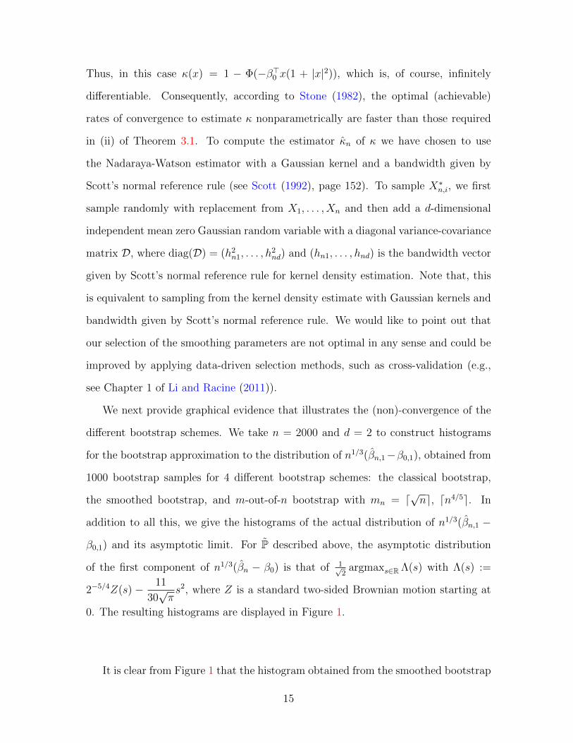
Thus, in this case κ(x) = 1 − Φ(−β>0 x(1 + |x|2)), which is, of course, infinitely

differentiable. Consequently, according to Stone (1982), the optimal (achievable)

rates of convergence to estimate κ nonparametrically are faster than those required

in (ii) of Theorem 3.1. To compute the estimator κn of κ we have chosen to use

the Nadaraya-Watson estimator with a Gaussian kernel and a bandwidth given by

Scott’s normal reference rule (see Scott (1992), page 152). To sample X∗n,i, we first

sample randomly with replacement from X1, . . . , Xn and then add a d-dimensional

independent mean zero Gaussian random variable with a diagonal variance-covariance

matrix D, where diag(D) = (h2n1, . . . , h

2nd) and (hn1, . . . , hnd) is the bandwidth vector

given by Scott’s normal reference rule for kernel density estimation. Note that, this

is equivalent to sampling from the kernel density estimate with Gaussian kernels and

bandwidth given by Scott’s normal reference rule. We would like to point out that

our selection of the smoothing parameters are not optimal in any sense and could be

improved by applying data-driven selection methods, such as cross-validation (e.g.,

see Chapter 1 of Li and Racine (2011)).

We next provide graphical evidence that illustrates the (non)-convergence of the

different bootstrap schemes. We take n = 2000 and d = 2 to construct histograms

for the bootstrap approximation to the distribution of n1/3(βn,1−β0,1), obtained from

1000 bootstrap samples for 4 different bootstrap schemes: the classical bootstrap,

the smoothed bootstrap, and m-out-of-n bootstrap with mn = d√ne, dn4/5e. In

addition to all this, we give the histograms of the actual distribution of n1/3(βn,1 −

β0,1) and its asymptotic limit. For P described above, the asymptotic distribution

of the first component of n1/3(βn − β0) is that of 1√2

argmaxs∈R Λ(s) with Λ(s) :=

2−5/4Z(s) − 11

30√πs2, where Z is a standard two-sided Brownian motion starting at

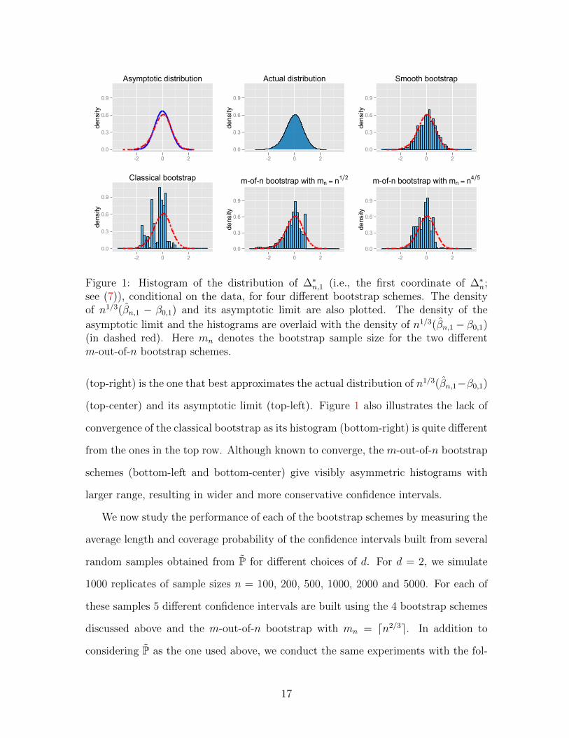
0. The resulting histograms are displayed in Figure 1.

It is clear from Figure 1 that the histogram obtained from the smoothed bootstrap

15

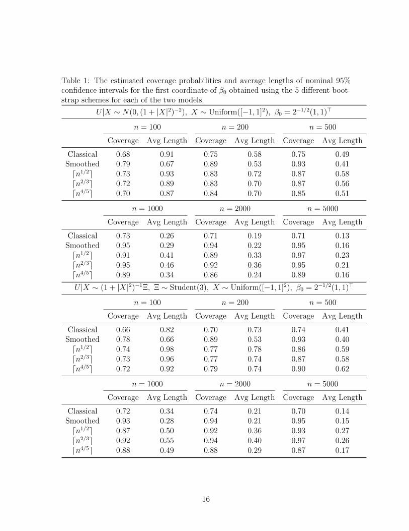
Table 1: The estimated coverage probabilities and average lengths of nominal 95%confidence intervals for the first coordinate of β0 obtained using the 5 different boot-strap schemes for each of the two models.

U |X ∼ N(0, (1 + |X|2)−2), X ∼ Uniform([−1, 1]2), β0 = 2−1/2(1, 1)>

n = 100 n = 200 n = 500

Coverage Avg Length Coverage Avg Length Coverage Avg Length

Classical 0.68 0.91 0.75 0.58 0.75 0.49Smoothed 0.79 0.67 0.89 0.53 0.93 0.41dn1/2e 0.73 0.93 0.83 0.72 0.87 0.58dn2/3e 0.72 0.89 0.83 0.70 0.87 0.56dn4/5e 0.70 0.87 0.84 0.70 0.85 0.51

n = 1000 n = 2000 n = 5000



U |X ∼ (1 + |X|2)−1Ξ, Ξ ∼ Student(3), X ∼ Uniform([−1, 1]2), β0 = 2−1/2(1, 1)>

n = 100 n = 200 n = 500



n = 1000 n = 2000 n = 5000



16

0.0

0.3

0.6

0.9

-2 0 2

density

Asymptotic distribution

0.0

0.3

0.6

0.9

-2 0 2

density

Actual distribution

0.0

0.3

0.6

0.9

-2 0 2

density

Smooth bootstrap

0.0

0.3

0.6

0.9

-2 0 2

density

Classical bootstrap

0.0

0.3

0.6

0.9

-2 0 2

density

m-of-n bootstrap with mn = n1 2

0.0

0.3

0.6

0.9

-2 0 2

density

m-of-n bootstrap with mn = n4 5

Figure 1: Histogram of the distribution of ∆∗n,1 (i.e., the first coordinate of ∆∗n;see (7)), conditional on the data, for four different bootstrap schemes. The densityof n1/3(βn,1 − β0,1) and its asymptotic limit are also plotted. The density of the

asymptotic limit and the histograms are overlaid with the density of n1/3(βn,1− β0,1)(in dashed red). Here mn denotes the bootstrap sample size for the two differentm-out-of-n bootstrap schemes.

(top-right) is the one that best approximates the actual distribution of n1/3(βn,1−β0,1)

(top-center) and its asymptotic limit (top-left). Figure 1 also illustrates the lack of

convergence of the classical bootstrap as its histogram (bottom-right) is quite different

from the ones in the top row. Although known to converge, the m-out-of-n bootstrap

schemes (bottom-left and bottom-center) give visibly asymmetric histograms with

larger range, resulting in wider and more conservative confidence intervals.

We now study the performance of each of the bootstrap schemes by measuring the

average length and coverage probability of the confidence intervals built from several

random samples obtained from P for different choices of d. For d = 2, we simulate

1000 replicates of sample sizes n = 100, 200, 500, 1000, 2000 and 5000. For each of

these samples 5 different confidence intervals are built using the 4 bootstrap schemes

discussed above and the m-out-of-n bootstrap with mn = dn2/3e. In addition to

considering P as the one used above, we conduct the same experiments with the fol-

17

lowing setting: U |X ∼ (1 + |X|2)−1Ξ, Ξ ∼ Student(3), X ∼ Uniform([−1, 1]2), β0 =

2−1/2(1, 1)> and Y = 1β>0 X+U≥0, where Student(3) stands for a standard Student-t

distribution with 3 degrees of freedom. The results are reported in Table 1.

Table 1 indicates that the smoothed bootstrap scheme outperforms all the others

as it achieves the best combination of high coverage and small average length. Its

average length is, overall, considerably smaller than those of the other consistent

procedures. Needless to say, the classical bootstrap performs poorly compared to the

others.

To study the effect of dimension on the performance of the 5 different bootstrap

schemes, we fix n = 10000 and sample from P for d = 3, 4, 5, and 6. For each d,

we consider 500 samples and for each sample we simulate 500 bootstrap replicates

to construct the confidence intervals. The results are summarized in Table 2. An

obvious conclusion of our simulation study is that the smoothed bootstrap is the best

choice.

It is easy to see from (3) that βn is the maximizer of a step function which is

not convex. Thus, the computational complexity of finding the maximum score es-

timator and that of bootstrap procedures increase with sample size and dimension;

see Manski and Thompson (1986), Pinkse (1993), and Florios and Skouras (2007) for

discussions on the computational aspect of the maximum score estimator. All sim-

ulations in this paper were done on a High Performance Computing (HPC) cluster

with Intel E5-2650L processors running R software over Red Hat Enterprise Linux.

For d = 6 and n = 10000, each of the 500 independent replications took an average

of 33 hours to evaluate the smoothed bootstrap confidence interval, while it took 23

hours to compute the classical bootstrap interval, and 3 hours for the m-out-of-n

bootstrap procedure with mn = n4/5. We would like to point out that the routine

implementing the different bootstrap procedures has not been optimized. Further-

more as bootstrap procedures are embarrassingly parallel, distributed computing can

18

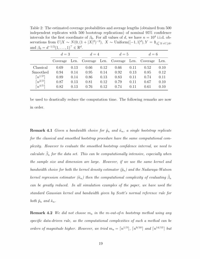
Table 2: The estimated coverage probabilities and average lengths (obtained from 500independent replicates with 500 bootstrap replications) of nominal 95% confidenceintervals for the first coordinate of β0. For all values of d, we have n = 104 i.i.d. ob-servations from U |X ∼ N(0, (1 + |X|2)−2), X ∼ Uniform([−1, 1]d), Y = 1β>0 X+U≥0,

and β0 = d−1/2(1, . . . , 1)> ∈ Rd.

d = 3 d = 4 d = 5 d = 6

Coverage Len. Coverage Len. Coverage Len. Coverage Len.

Classical 0.69 0.13 0.66 0.12 0.66 0.11 0.52 0.10Smoothed 0.94 0.14 0.95 0.14 0.92 0.13 0.85 0.12dn1/2e 0.89 0.14 0.86 0.13 0.83 0.11 0.74 0.11dn2/3e 0.87 0.13 0.81 0.12 0.79 0.11 0.67 0.10dn4/5e 0.82 0.13 0.76 0.12 0.74 0.11 0.61 0.10

be used to drastically reduce the computation time. The following remarks are now

in order.

Remark 4.1 Given a bandwidth choice for pn and κn, a single bootstrap replicate

for the classical and smoothed bootstrap procedure have the same computational com-

plexity. However to evaluate the smoothed bootstrap confidence interval, we need to

calculate βn for the data set. This can be computationally intensive, especially when

the sample size and dimension are large. However, if we use the same kernel and

bandwidth choice for both the kernel density estimator (pn) and the Nadaraya-Watson

kernel regression estimator (κn) then the computational complexity of evaluating βn

can be greatly reduced. In all simulation examples of the paper, we have used the

standard Gaussian kernel and bandwidth given by Scott’s normal reference rule for

both pn and κn.

Remark 4.2 We did not choose mn in the m-out-of-n bootstrap method using any

specific data-driven rule, as the computational complexities of such a method can be

orders of magnitude higher. However, we tried mn = dn1/3e, dn9/10e and dn14/15e but

19

their results were inferior to the reported choices (dn1/2e, dn2/3e and dn4/5e). Further-

more, we would like to point out that finite sample performance of smoothed bootstrap

is superior to that of those obtained by Delgado et al. (2001) using subsampling (sam-

pling without replacement) bootstrap methods.

5 A convergence theorem

We now present a convergence theorem for triangular arrays of random variables

arising from the binary choice model discussed above. This theorem will be used in

Section 6 to prove Theorem 3.1.

Suppose that we are given a probability space (Ω,A,P) and a triangular array of

random variables (Xn,j, Yn,j)n∈N1≤j≤mn where (mn)∞n=1 is a sequence of natural numbers

satisfying mn ↑ ∞ as n→∞, and Xn,j and Yn,j are Rd and 0, 1-valued random vari-

ables, respectively. Furthermore, assume that the rows (Xn,1, Yn,1), . . . , (Xn,mn , Yn,mn)

are formed by i.i.d. random variables. We denote the distribution of (Xn,j, Yn,j),

1 ≤ j ≤ mn, n ∈ N, by Qn and the density of Xn,j by pn. Recall the probability

measure P on Rd+1 and the notation introduced in Section 2. Denote by P∗n the em-

pirical measure defined by the row (Xn,1, Yn,1), . . . , (Xn,mn , Yn,mn). Consider the class

of functions

F :=

fα(x, y) :=

(y − 1

2

)1α>x≥0 : α ∈ Rd

, (12)

G :=

gβ(x) :=

(κ(x)− 1

2

)1β>x≥0 : β ∈ Rd

. (13)

We will say that β∗n ∈ Sd−1 is a maximum score estimator based on (Xn,i, Yn,i),

1 ≤ i ≤ mn, if

β∗n = argmaxβ∈Sd−1

1

mn

mn∑i=1

(Yn,i −

1

2

)1β>Xn,i≥0 = argmax

β∈Sd−1

P∗n(fβ),

20

where fβ is defined in (12). For any set Borel set A ⊂ Rd, let νn(A) :=∫Apn(x)dx. We

take the measures Qnn∈N and densities pnn∈N to satisfy the following conditions:

(A1) ‖Qn − P‖G → 0 and the sequence νn∞n=1 is uniformly tight. Moreover, pn

is continuously differentiable on X and ∇pn is integrable (with respect to the

Lebesgue measure) over X.

(A2) For each n ∈ N there is a continuously differentiable function κn : X → [0, 1]

such that

κn(x) = Qn(Y = 1|X = x)

for all n ∈ N, and ‖κn − κ‖X → 0 for every compact set X ⊂ X.

For n ∈ N, define Γn : Rd → R as

Γn(β) := Qn (fβ) =

∫ (κn(x)− 1

2

)1β>x≥0 pn(x) dx. (14)

(A3) Assume that

βn := argmaxβ∈Sd−1

Γn(β), (15)

exists for all n, and

∫β>n x=0

(∇κn(x)>βn) pn(x)xx> dσβn →∫β>0 x=0

(∇κ(x)>β0) p(x)xx> dσβ0 , (16)

where the above terms are standard surface integrals and σβn denotes the surface

measure over x ∈ Rd : β>n x = 0, for all n ≥ 0.

Let Fn,K be a measurable envelope of the class of functions

Fn,K := 1β>x≥0 − 1β>n x≥0 : |β − βn| ≤ K.

21

Note that there are two small enough constants C,K∗ > 0 such that for any 0 < K ≤

K∗ and n ∈ N, Fn,K can be taken to be of the form 1β>Kx≥0>α>Kx+ 1α>Kx≥0>β>Kx

for

αK , βK ∈ Rd satisfying |αK − βK | ≤ CK.

(A4) Assume that there exist R0,∆0 ∈ (0, K∗ ∧ 1] and a decreasing sequence εn∞n=1

of positive numbers with εn ↓ 0 such that for any n ∈ N and for any ∆0m−1/3n <

R ≤ R0 we have

(i) |(Qn − P)(F 2n,R)| ≤ ε1R;

(ii) sup|α−βn|∨|β−βn|≤R

|α−β|≤R

∣∣(Qn − P)(1α>X≥0 − 1β>X≥0)∣∣ ≤ εnRm

−1/3n .

In Lemma A.1, we show that conditions (A1)–(A3) imply that Γn, as defined in

(14), is twice continuously differentiable in a neighborhood of βn. The main properties

of Γ and Γn are established in Lemma A.1 of the appendix.

5.1 Consistency and rate of convergence

In this sub-section we study the asymptotic properties of β∗n. Before attempting to

prove any asymptotic results, we will state the following lemma, proved in Section 7,

which establishes an important relationship between the βn’s, defined in (15), and β0.

Lemma 5.1 Under (A1) and (A2), we have βn → β0.

In the following lemma, proved in Section 7, we show that β∗n is a consistent estimator

of β0.

Lemma 5.2 If (A1) and (A2) hold, β∗nP−→ β0.

We will now deduce the rate of convergence of β∗n. It will be shown that β∗n converges at

rate m−1/3n . The proof of this fact relies on empirical processes arguments like those

used to prove Lemma 4.1 in Kim and Pollard (1990). The following two lemmas,

22

proved in Section 7, adopt these ideas to our context (a triangular array in which

variables in the same row are i.i.d.). The first lemma is a maximal inequality specially

designed for this situation.

Lemma 5.3 Under (A1), (A2), and (A4), there is a constant CR0 > 0 such that

for any R > 0 and n ∈ N such that ∆0m−1/3n ≤ Rm

−1/3n ≤ R0 we have

E

(sup

|βn−β|≤Rm−1/3n

|(P∗n −Qn)(fβ − fβn)|2

)≤ CR0Rm

−4/3n ∀ n ∈ N.

With the aid of Lemma 5.3 we can now derive the rate of convergence of the

maximum score estimator.

Lemma 5.4 Under (A1), (A2), and (A4), m1/3n (β∗n − βn) = OP(1).

5.2 Asymptotic distribution

Before going into the derivation of the limit law of β∗n, we need to introduce some

further notation. Consider a sequence of matrices (Hn)∞n=1 ⊂ Rd×(d−1) and H ∈

Rd×(d−1) satisfying the following properties:

(a) ξ 7→ Hnξ and ξ 7→ Hξ are bijections from Rd−1 to the hyperplanes x ∈ Rd :

β>n x = 0 and x ∈ Rd : β>0 x = 0, respectively.

(b) The columns of Hn and H form orthonormal bases for x ∈ Rd : β>n x = 0 and

x ∈ Rd : β>0 x = 0, respectively.

(c) There is a constant CH > 0, depending only on H, such that ‖Hn − H‖2 ≤

CH |βn − β0|.

We now give an intuitive argument for the existence of such a sequence of matrices.

Imagine that we find an orthonormal basis e0,1, . . . , e0,d−1 for the hyperplane x ∈

Rd : β>0 x = 0 and we let H have these vectors as columns. We then obtain the rigid

23

motion T : Rd → Rd that moves β0 to βn and the hyperplane x ∈ Rd : β>0 x = 0 to

x ∈ Rd : β>n x = 0. We let the columns of Hn be given by T e0,1, . . . , T e0,d−1. The

resulting sequence of matrices will satisfy the (a), (b) and (c) for some constant CH .

Note that (b) implies that H>n and H> are the Moore-Penrose pseudo-inverses

of Hn and H, respectively. In particular, H>nHn = H>H = Id−1, where Id−1 is the

identity matrix in Rd−1 (in the sequel we will always use this notation for identity

matrices on Euclidean spaces). Additionally, it can be inferred from (b) that H>n (Id−

βnβ>n ) = H>n and H>(Id − β0β

>0 ) = H>. Now, for each s ∈ Rd−1 define

βn,s :=

(√1− (m

−1/3n |s|)2 ∧ 1 βn +m−1/3

n Hns

)1|s|≤m1/3

n+ |s|−1Hns1|s|>m1/3

n. (17)

Note that βn,s ∈ Sd−1 as β>nHns = 0 and |Hns| = |s| for all s ∈ Rd−1. Also, as

s varies in the set |s| < m1/3n , βn,s takes all values in the set β ∈ Sd−1 : β>n β >

0. Furthermore, if |s| ≤ m1/3n , Hns is the orthogonal projection of βn,s onto the

hyperplane x ∈ Rd : β>n x = 0; otherwise βn,s is orthogonal to βn. Define the

process

Λn(s) := m2/3n P∗n(fβn,s − fβn)

and

s∗n := argmaxs∈Rd−1

Λn(s) = argmaxs∈Rd−1

P∗n(fβn,s).

Recall that β∗n = argmaxβ∈Sd−1 P∗nfβ. As β∗n converges to βn, β∗n will belong to the

set β ∈ Sd−1 : β>n β > 0 with probability tending to one. Thus, βn,s∗n = β∗n and

|s∗n| < m1/3n with probability tending to one, as n→∞. Note that by (17), we have

β∗n =

√1− (m

−1/3n s∗n)2 ∧ 1 βn +m−1/3

n Hns∗n,

24

when |s∗n| < m1/3n . Rearranging the terms in the above display, we get

s∗n = m1/3n H>n (β∗n − βn) +m1/3

n

[√1− (m

−1/3n s∗n)2 ∧ 1− 1

]H>n βn,

when |s∗n| < m1/3n . As H>n βn = 0 (from the defintion of Hn), we have

s∗n = m1/3n H>n (β∗n − βn), (18)

with probability tending to 1, as n→∞. Considering this, we will regard the processes

Λnn≥1 as random elements in the space of locally bounded real-valued functions on

Rd−1 (denoted by Bloc(Rd−1)) and then derive the limit law of s∗n by applying the

argmax continuous mapping theorem. We will take the space Bloc(Rd−1) with the

topology of uniform convergence on compacta; our approach is based on that of Kim

and Pollard (1990).

To properly describe the asymptotic distribution we need to define the function

Σ : Rd−1 × Rd−1 → R as follows:

Σ(s, t) :=1

4

∫Rd−1

[(s>ξ) ∧ (t>ξ)]+ + [(s>ξ) ∨ (t>ξ)]−p(Hξ) dξ

=1

8

∫Rd−1

(|s>ξ|+ |t>ξ| − |(s− t)>ξ|)p(Hξ) dξ.

Additionally, denote by Wn the Bloc(Rd−1)-valued process given by

Wn(s) := m2/3n (P∗n −Qn)(fβn,s − fβn).

In what follows, the symbol will denote convergence in distribution. We are now

in a position to state and prove our convergence theorem.

Theorem 5.1 Assume that (A1)–(A4) hold. Then, there is a Bloc(Rd−1)-valued

stochastic process Λ of the form Λ(s) = W (s)+ 12s>H>∇2Γ(β0)Hs, where W is a zero-

25

mean Gaussian process in Bloc(Rd−1) with continuous sample paths and covariance

function Σ. Moreover, Λ has a unique maximizer w.p. 1 and we have

(i) Λn Λ in Bloc(Rd−1),

(ii) s∗n s∗ := argmaxs∈Rd−1

Λ(s),

(iii) m1/3n (β∗n − βn) Hs∗.

Proof: Lemmas A.3 and A.4 imply that the sequence (Wn)∞n=1 is stochastically

equicontinuous and that its finite dimensional distributions converge to those of a

zero-mean Gaussian process with covariance Σ. From Theorem 2.3 in Kim and

Pollard (1990) we know that here exists a continuous process W with these prop-

erties and such that Wn W . By definition of Γn, note that Λn(·) = Wn(·) +

m2/3n (Γn(βn,(·)) − Γn(βn)). Moreover, from Lemma A.1, we have m

2/3n (Γn(βn,(·)) −

Γn(βn))P−→ 1

2(·)>H>∇2Γ(β0)H(·) on Bloc(Rd−1) (with the topology of uniform conver-

gence on compacta). Thus, applying Slutsky’s lemma (see e.g., Example 1.4.7, page

32 in van der Vaart and Wellner (1996)) we get that Λn Λ. The uniqueness of

the maximizers of the sample paths of Λ follows from Lemmas 2.5 and 2.6 in Kim

and Pollard (1990). Finally an application of Theorem 2.7 in Kim and Pollard (1990)

gives (ii), and (iii) follows from (18).

As a corollary we immediately obtain the asymptotic distribution of the maximum

score estimator (taking κn ≡ κ and βn ≡ β0) computed from i.i.d. samples from P.

Corollary 5.1 If (Xn, Yn)∞n=1i.i.d.∼ P and βn is a maximum score estimator computed

from (Xi, Yi)ni=1, for every n ≥ 1, then,

n1/3(βn − β0) H argmaxs∈Rd−1

Λ(s).

26

One final remark is to be made about the process Λ. The quadratic drift term can

be rewritten, by using the matrix H to evaluate the surface integral, to obtain the

following more convenient expression

Λ(s) = W (s)− 1

2s>(∫

Rd−1

(∇κ(Hξ)>β0)p(Hξ)ξξ> dξ

)s.

Remark: Theorem 5.1 gives us a general framework to prove the consistency of any

bootstrap scheme. For example, if Qn is an estimator of P, computed from the data,

such that (A1)–(A4) hold in probability or a.s. (see the proof of Theorem 3.1), then

the bootstrap scheme which generates bootstrap samples from Qn will be consistent.

6 Proof of Theorem 3.1

In this section we use Theorem 5.1 to prove Theorem 3.1. We set κn = κn, βn =

βn. Let nk be a subsequence of N. We will show that there exists a further

subsequence nkl such that conditional on the data Z , ρ(Gnkl,G)

a.s.→ 0. To show that

ρ(Gnkl,G) → 0 a.e. data (X1, Y1), . . . , (Xn, Yn) we appeal to Theorem 5.1. To apply

Theorem 5.1 we need to show that conditions (A1)–(A4) hold along the subsequence

nkl for a.e. (X1, Y1), . . . , (Xn, Yn).

First observe that (S2) implies that (A2) holds along nkl a.s. We first show

that ‖Qn − P‖GP→ 0. Observe that by assumption (S1),

|(Qn − P)(gβ(X))| =∣∣∣∣∫

X

(κ(x)− 1

2

)1β>x≥0(pn(x)− p(x)) dx

∣∣∣∣ ≤ ‖pn − p‖X P−→ 0.

As pn converges to p uniformly, νn converges and is thus uniformly tight. This shows

that (A1) holds along a further subsequence of nk for a.e. data sequence. Next we

will show that (A3) hold in probability and the probability that inequalities (A4)

(i)–(ii) holds tend to 1 as n→∞.

27

We will now show that (16) holds in probability with κn = κn, pn = pn and

βn = βn. The proof of (A3) is slightly more involved and we describe the details

below. Without loss of generality2 we can assume that X is the closed unit ball in Rd

and write Xρ := (1− ρ)X, for any 0 < ρ < 1. By triangle inequality

∥∥∥∥∥∫β>n x=0

(∇κn(x)>βn)pn(x)xx>dσβn −∫β>0 x=0

(∇κ(x)>β0)p(x)xx>dσβ0

∥∥∥∥∥2

≤ Un + Zn + Vn

where

Un :=

∥∥∥∥∫β>n x=0

(∇κn(x)−∇κ(x))>βnpn(x)xx> dσβn

∥∥∥∥2

,

Zn :=

∥∥∥∥∫β>n x=0

∇κ(x)>βn(pn(x)− p(x))xx> dσβn

∥∥∥∥2

, and

Vn :=

∥∥∥∥∥∫β>n x=0

(∇κ(x)>βn) p(x)xx> dσβn −∫β>0 x=0

(∇κ(x)>β0) p(x)xx> dσβ0

∥∥∥∥∥2

.

Consider the matrices H and (Hn)∞n=1 described at the beginning of Section 5.2. Then

Vn can be expressed as

∥∥∥∥∫Rd−1

(∇κ(Hnξ)>βn) p(Hnξ)Hnξξ

>H>n dξ −∫Rd−1

(∇κ(Hξ)>β0) p(Hξ)Hξξ>H> dξ

∥∥∥∥2

.

As p has compact support (both ∇κ and p are bounded) and the Hn’s are linear

isometries, we can apply the dominated convergence theorem to show that the above

display goes to zero w.p. 1. Note that βn and thus Hn’s converge to β0 and H, respec-

tively, w.p. 1 as a consequence of Lemma 5.1 and observation (c) in the beginning of

Section 5.2.

2For a general convex compact set X with non-empty interior define R∗ := supR > 0 : ∂B(0, R)∩X 6= ∅, where ∂B(0, R) is the boundary of the ball of radius R around 0 in Rd. For any 0 < ρ < R∗,take Xρ := X ∩B(0, R∗ − ρ). The proof would now follow with appropriate changes in the domainsof integration.

28

On the other hand, Un is bounded from above by

‖∇κn −∇κ‖X ‖pn‖X∫

β>n x=01−ρ≤|x|≤1

|x|2 dσβn + ‖∇κn −∇κ‖Xρ ‖pn‖X∫β>n x=0|x|≤1

|x|2 dσβn .

From the results in Blondin (2007) we know that ‖∇κn(x) − ∇κ(x)‖Xρa.s.→ 0. Thus,

noting that these surface integrals are βn-invariant, we get

Un ≤ ‖∇κn −∇κ‖X ‖pn‖X∫

β>0 x=01−ρ≤|x|≤1

|x|2 dσβ0 + oP(1).

For any ε > 0 we can choose Mε large enough, and ρε sufficiently small so that

supn≥1

P(‖∇κn −∇κ‖X > Mε

)<ε

2and Mε(‖p‖X + op(n

−1/3))

∫β>0 x=0

1−ρε≤|x|≤1

|x|2 dσβ0 <ε

2.

Thus for all sufficiently large n ∈ N,

P(Un > ε) ≤ P(‖∇κn −∇κ‖X > Mε) + P(Un > ε, ‖∇κn −∇κ‖X ≤Mε) < ε.

Finally, Zn can be bounded from above as

∥∥∥∥∫β>n x=0

∇κ(x)>βn(pn(x)− p(x))xx> dσβn

∥∥∥∥2

≤ ‖∇κ‖X‖pn − p‖X∫β>n x=0|x|≤1

|x|2 dσβn = op(n−1/3).

To see that (A4) holds, we will first show (A4)-(ii). Observe that the set x ∈ Rd :

α>x ≥ 0 > β>x is a multi-dimensional wedge-shaped region in Rd, which subtends

an angle of order |α − β| at the origin. As X is a compact subset of Rd (assumption

(C1)), we have that ∫X

|1α>x≥0 − 1β>x≥0| dx . |α− β|,

29

where by . we mean bounded from above by a constant multiple; also see Example

6.4, page 214 of Kim and Pollard (1990). Thus, for any α, β ∈ Rd, we have

|(Qn − P)(1α>X≥0 − 1β>X≥0)|

=

∣∣∣∣∫X

(1α>x≥0 − 1β>x≥0)(pn(x)− p(x)) dx

∣∣∣∣. |α− β|‖pn − p‖X.

It is now straightforward to show that (A4)-(ii) will hold in probability because

‖pn − p‖X = oP(n−1/3). A similar argument gives (A4)-(i).

7 Proofs of results in Section 5.1

7.1 Proof of Lemma 5.1

Let ε > 0 and consider a compact set Xε such that Qn(Xε × R) > 1 − ε for all n ∈ N

(its existence is guaranteed by (A1)). Then,

|Γn(β)−Qn(gβ)| ≤ 2Qn((Rd \ Xε)× R) + ‖κn − κ‖Xε

for all β ∈ Sd−1, where gβ is defined in (13). Consequently, (A2) shows that

lim ‖Γn(β)−Qn(gβ)‖Sd−1 ≤ 2ε. Moreover, from (A1), we have that ‖Qn − P‖G → 0.

Therefore, as ε > 0 is arbitrary and Γ(β) = P(gβ), we have

‖Γn − Γ‖Sd−1 → 0. (19)

Considering that β0 is the unique maximizer of the continuous function Γ we can

conclude the desired result as βn maximizes Γn and the argmax function is contin-

uous (under the sup-norm) for continuous functions on compact spaces with unique

30

maximizers.


Recall that β0 is the well-separated unique maximizer of P(fβ) ≡ Γ(β). Thus, the

result would follow as a simple consequence of the argmax continuous mapping theo-

rem (see e.g., Corollary 3.2.3, van der Vaart and Wellner (1996)) if we can show that

‖(P∗n − P)(fβ)‖Sd−1P−→ 0. As

‖(P∗n − P)(fβ)‖Sd−1 ≤ ‖(P∗n −Qn)(fβ)‖Sd−1 + ‖Γn − Γ‖Sd−1 ,

in view of (19), it is enough to show that E (‖P∗n −Qn‖F) → 0. Now consider the

classes of functions F1 := y1α>x≥0 : α ∈ Rd and F2 := 1α>x≥0 : α ∈ Rd.

Note that as F = F1 − 12F2, it follows that E (‖P∗n −Qn‖F) ≤ E (‖P∗n −Qn‖F1) +

E (‖P∗n −Qn‖F2) . Furthermore, observe that both F1 and F2 have the constant one as

a measurable envelope function. The proof of the lemma would be complete if we can

show the classes of functions F1 and F2 are manageable in the sense of definition 4.1 of

Pollard (1989), as by corollary 4.3 of Pollard (1989) we will have E (‖P∗n −Qn‖Fi) ≤

Ji/√mn for i = 1, 2, where the constants J1 and J2 are positive and finite. As VC-

subgraph classes of functions with bounded envelope are manageable, we will next

show that both F1 and F2 are VC-subgraph classes of functions. Since the class of

all half-spaces of Rd+1 is VC (see Exercise 14, page 152 in van der Vaart and Wellner

(1996)), Lemma 2.6.18 in page 147 of van der Vaart and Wellner (1996) implies that

both F1 = y1α>x≥0 : α ∈ Rd and F2 are VC-subgraph classes of functions.


Take R0 ≤ K∗, so for any K ≤ R0 the class fβ − fβn|β−βn|<K is majorized by Fn,K .

Our assumptions on P then imply that there is a constant C such that P(F 2n,K) =

31

P(Fn,K) ≤ CCK for 0 < K ≤ K∗ (recall that Fn,K is an indicator function). Note

that the last inequality follows as (α, β) 7→ P(β>X ≤ 0 < α>X) is continuously

differentiable around (βn, βn) (which can be shown using similar ideas as in Lemma

A.1), and thus locally Lipschitz. Now, take R > 0 and n ∈ N such that ∆0m−1/3n <

Rm−1/3n ≤ R0. Since F

n,Rm−1/3n

is a VC-class (with VC index bounded by a constant

independent of n and R), the maximal inequality 7.10 in page 38 of Pollard (1990)

implies the existence of a constant J , not depending neither on mn nor on R, such

that

E

(‖P∗n −Qn‖2

Fn,Rm

−1/3n

)≤ JQn(F

n,Rm−1/3n

) m−1n .

From (A4)-(i) we can conclude that

E

(‖P∗n −Qn‖2

Fn,Rm

−1/3n

)≤ J(O(m−1/3

n ) + CCRm−1/3n ) m−1

n

for all R and n for which m−1/3n R ≤ R0. This finishes the proof.


Take R0 as in (A4), let ε > 0 and define

Mε,n := inf

a > 0 : sup|β−βn|≤R0

β∈Sd−1

|(P∗n −Qn)(fβ − fβn)| − ε|β − βn|2 ≤ am−2/3n

;

Bn,j :=β ∈ Sd−1 : (j − 1)m−1/3n < |β − βn| ≤ jm−1/3

n ∧R0.

32

Then, by Lemma 5.3 we have

P (Mε,n > a)

= P(∃ β ∈ Sd−1, |β − βn| ≤ R0 : |(P∗n −Qn)(fβ − fβn)| > ε|β − βn|2 + a2m−2/3

n

)≤

∞∑j=1

P(∃ β ∈ Bn,j : m2/3

n |(P∗n −Qn)(fβ − fβn)| > ε2(j − 1)2 + a2)

≤∞∑j=1

m4/3n

(ε(j − 1)2 + a2)2E

(sup

|βn−β|<jm−1/3n ∧R0

|(P∗n −Qn)(fβ − fβn)|2

)

≤ CR0

∞∑j=1

j

(ε(j − 1)2 + a2)2→ 0 as a→∞.

It follows that Mε,n = OP(1). From Lemma A.1-(c) we can find N ∈ N and R, ε > 0

such that Γn(β) ≤ Γn(βn) − 2ε|β − βn|2 for all n ≥ N and β ∈ Sd−1 such that

0 < |β − βn| < R. Since Lemma 5.2 implies β∗n − βnP−→ 0, with probability tending

to one we have

P∗n(fβ∗n − fβn) ≤Qn(fβ∗n − fβn) + ε|β∗n − βn|2 +M2ε,nm

−2/3n

≤Γn(β∗n)− Γn(βn) + ε|β∗n − βn|2 +M2ε,nm

−2/3n

≤− ε|β∗n − βn|2 +M2ε,nm

−2/3n .

Therefore, since β∗n is a maximum score estimator and Mε,n = OP(1) we obtain

that ε|β∗n − βn|2 ≤ 32εn|β∗n − βn|m

−1/3n +OP(m

−2/3n ). This finishes the proof.

8 Acknowledgement

The third author would like to thank Jason Abrevaya for suggesting him the problem.

We would also like to thank the Associate Editor and two anonymous referees for their

helpful and constructive comments.

33

A Auxiliary results for the proof of Theorem 5.1

Lemma A.1 Denote by σβ the surface measure on the hyperplane x ∈ Rd : β>x =

0. For each α, β ∈ Rd \ 0 define the matrix Aα,β := (Id − |β|−2ββ>)(Id −

|α|−2αα>) + |β|−1|α|−1βα>. Note that, x 7→ Aα,βx maps the region α>x ≥ 0 to

β>x ≥ 0, taking α>x = 0 onto β>x = 0. Recall the definitions of Γn (see (14))

and Γ (see (4)). Then,

(a) β0 is the only maximizer of Γ on Sd−1 and we have

∇Γ(β) =β>β0

|β|2

(Id −

1

|β|2ββ>

)∫β>0 x=0

(κ(Aβ0,βx)− 1

2

)p(Aβ0,βx)x dσβ0 ,

∇2Γ(β0) =−∫β>0 x=0

(∇κ(x)>β0) p(x)xx> dσβ0 .

Furthermore, there is an open neighborhood U ⊂ Rd of β0 such that β>∇2Γ0(β0)β <

0 for all β ∈ U \ tβ0 : t ∈ R.

(b) Under (A1)–(A3), we have

∇Γn(β) =β>βn|β|2

(Id −

1

|β|2ββ>

)∫β>n x=0

(κn(Aβn,βx)− 1

2

)pn(Aβn,βx)x dσβn ,

∇2Γn(βn) =−∫β>n x=0

(∇κn(x)>βn) pn(x)xx> dσβn .

(c) If conditions (A1)–(A3) hold, then ∇2Γn(βn)→ ∇2Γ(β0). Consequently, there

is N ≥ 0 and a subset U ⊂ U such that for any n ≥ N , βn is a strict local

maximizer of Γn on Sd−1 and β>∇2Γn(βn)β < 0 for all β ∈ U \ tβn : t ∈ R.

Proof: We start with (a). Lemma 2 in Manski (1985) implies that β0 is the

only minimizer of Γ on Sd−1. The computation of ∇Γ and ∇2Γ are based on those

in Example 6.4 in page 213 of Kim and Pollard (1990). Note that for any x with

β>0 x = 0 we have ∇κ(x)>β0 ≥ 0 (because for x orthogonal to β0, κ(x + tβ0) ≤ 1/2

34

and κ(x + tβ0) ≥ 1/2 whenever t < 0 and t > 0, respectively). Additionally, for any

β ∈ Rd we have:

β>∇2Γ(β0)β = −∫β>0 x=0

(∇κ(x)>β0)(β>x)2p(x) dσβ0 .

Thus, the fact that the set x ∈ X : (∇κ(x)>β0)p(x) > 0 is open (as p and ∇κ are

continuous) and intersects the hyperplane x ∈ Rd : β>0 x = 0 implies that ∇2Γ(β0)

is negative definite on a set of the form U \ tβ0 : t ∈ R with U ⊂ Rd being an open

neighborhood of β0.

We now prove (b) and (c). By conditions (A1) and (A2) we have that κn is

continuously differentiable on X and ∇pn is integrable on X. Thus, we can compute

∇Γn by an application of the divergence theorem as in Example 6.4 in page 213 of

Kim and Pollard (1990). By the change of variable formula for measures (see Theorem

16.13, page 216 of Billingsley (1995)), we can express ∇Γn(β) as

β>n β0β>βn|β|2

(Id −

1

|β|2ββ>

)∫β>0 x=0

(κn(Aβn,βAβ0,βnx)− 1

2

)pn(Aβn,βAβ0,βnx)Aβ0,βnx dσβ0 .

Starting with the above expression for ∇Γn we take the derivative with respect to

β using the product rule and differentiate under the integral sign. Recall that βn

maximizes Γn(·), i.e., ∇Γn(βn) = 0. Thus, one of the terms in ∇2Γn(βn) will be zero

as (note that Aβn,βn = Id)

∫β>0 x=0

(κn(Aβ0,βnx)− 1

2

)pn(Aβ0,βnx)Aβ0,βnx dσβ0 = 0.

Hence, the only non-zero term in ∇2Γn(βn) is −∫β>n x=0

(∇κn(x)>βn)pn(x)xx>dσβn .

Part (c) now follows immediately from (b) and condition (A3).

Lemma A.2 Let R > 0. Under (A1)–(A4) there is a sequence of random variables

35

∆Rn = OP(1) such that for every δ > 0 and every n ∈ N we have,

sup|s−t|≤δ|s|∨|t|≤R

P∗n[(fβn,s − fβn,t)2

]≤ δ∆R

nm−1/3n .

Proof: Define GnR,δ := fβn,s − fβn,t : |s − t| ≤ δ, |s| ∨ |t| ≤ R and GnR :=

fβn,s − fβn,t : |s| ∨ |t| ≤ R. It can be shown that GnR is manageable with envelope

Gn,R := 3Fn,2Rm

−1/3n

(as |κn−1/2| ≤ 1). Note that Gn,R is independent of δ. Moreover,

our assumptions on P then imply that there is a constant C such that P(F 2n,K) =

P(Fn,K) ≤ CCK for 0 < K ≤ K∗, where the first equality is true because Fn,K is

an indicator function (see proof of Lemma 5.3 for more detail). Considering this,

condition (A4)-(i) implies that

QnG2n,R .

∣∣(Qn − P)(F 2

n,2Rm−1/3n

)∣∣+∣∣P(F 2

n,2Rm−1/3n

)∣∣

. ε12Rm−1/3n + 2Rm−1/3

n = O(m−1/3n ).

Thus, (A4)-(ii) and the maximal inequality 7.10 from Pollard (1990) show that there

is a constant JR such that for all large enough n we have

E



]≤ 2E


P∗n(|fβn,s − fβn,t |

)≤ 2E

(supf∈GnR

(P∗n −Qn)|f |

)+ 2 sup

f∈GnR,δQn|f |

≤ m−1/2n 4ε1JR

√QnG2

n,R + 2 supf∈GnR

∣∣(Qn − P)|f |∣∣+ 2 sup

f∈GnR,δP|f |

≤ mn−1/24ε1JR

√O(m

−1/3n ) +

2εnR

m1/3n

+ 2 supf∈GnR,δ

P|f |.

36

On the other hand, our assumptions on P imply that the function P(1(·)>x≥0) is

continuously differentiable, and hence Lipschitz, on Sd−1. Thus, there is a constant

L, independent of δ, such that

E



] ≤ o(m−1/3n ) + δLm−1/3

n .

The result now follows.

Lemma A.3 Under (A1)–(A4), for every R, ε, η > 0 there is δ > 0 such that

limn→∞

P


m2/3n

∣∣(P∗n −Qn)(fβn,s − fβn,t)∣∣ > η

≤ ε.

Proof: Let Ψn := m1/3n P∗n(4F 2

n,Rm−1/3n

) = m1/3n P∗n(F

n,Rm−1/3n

). Note that our assump-

tions on P then imply that there is a constant C such that P(F 2n,K) = P(Fn,K) ≤ CCK

for 0 < K ≤ K∗ (Fn,K is an indicator function). Considering this, conditions (A4)-(i)

and Lemma 5.3 imply that

E (Ψn) =m1/3n Qn

(P∗nFn,Rm−1/3

n

)=m1/3

n QnFn,Rm−1/3n

=m1/3n (Qn − P)(F

n,Rm−1/3n

) +m1/3n P(F

n,Rm−1/3n

) = O(1).

Now, define

Φn := m1/3n sup

|s−t|≤δ|s|∨|t|≤R

P∗n((fβn,s − fβn,t)2

).

The class of all differences fβn,s− fβn,t with |s| ∨ |t| ≤ R and |s− t| < δ is manageable

(in the sense of definition 7.9 in page 38 of Pollard (1990)) for the envelope function

37

2Fn,Rm

−1/3n

. By the maximal inequality 7.10 in Pollard (1990), there is a continuous

increasing function J with J(0) = 0 and J(1) <∞ such that

E


∣∣(P∗n −Qn)(fβn,s − fβn,t)∣∣ ≤ 1

m2/3n

Qn

(√ΨnJ (Φn/Ψn)

).

Let ρ > 0. Breaking the integral on the right on the events that Ψn ≤ ρ and Ψn > ρ

and the applying Cauchy-Schwartz inequality,

E


m2/3n

∣∣(P∗n −Qn)(fβn,s,βn − fβn,t,βn)∣∣

≤ √ρJ(1) +√

E (Ψn1Ψn>ρ)√E (J (1 ∧ (Φn/ρ))),

≤ √ρJ(1) +√

E (Ψn1Ψn>ρ)√E (J (1 ∧ (δ∆R

n /ρ))),

where ∆Rn = OP(1) is as in Lemma A.2. It follows that for any given R, η, ε > 0 we

can choose ρ and δ small enough so that the results holds.

Lemma A.4 Let s, t, s1, . . . , sN ∈ Rd−1 and write ΣN ∈ RN×N for the matrix given

by ΣN := (Σ(sk, sj))k,j. Then, under (A1)–(A4) we have

(a) m1/3n Qn(fβn,s − fβn)→ 0,

(b) m1/3n Qn

((fβn,s − fβn)(fβn,t − fβn)

)→ Σ(s, t),

(c) (Wn(s1), . . . ,Wn(sN))> N(0,ΣN),

where N(0,ΣN) denotes an RN -valued Gaussian random vector with mean 0 and co-

variance matrix ΣN and stands for weak convergence.

Proof: (a) First note that for large enough mn, by (17), we have

m1/3n |βn,s − βn| ≤

∣∣∣√m2/3n − s2 −m1/3

n

∣∣∣+ |s| ≤ 2|s|,

38

where the second inequality is true as b− a ≤√b2 − a2, when b ≥ a ≥ 0 and the fact

that |Hns| = |s|. Moreover, we have that |βn,s − βn| → 0 and mn →∞. Now as βn is

the maximizer of Γn, observe that by (14), we have

m1/3n Qn(fβn,s − fβn) = m1/3

n (Γn(βn,s)− Γn(βn))

= m1/3n

[∇Γn(βn)>(βn,s − βn) +O(|βn,s − βn|2)

]= O(m1/3

n |βn,s − βn|2)

= O(|βn,s − βn|) = o(1).

(b) First note that (1U+β>nX≥0 − 1/2)2 ≡ 1/4 and

(1β>n,sx≥0 − 1β>n x≥0)(1β>n,tx≥0 − 1β>n x≥0) = 1(β>n,sx)∧(β>n,tx)≥0>β>n x+ 1β>n x≥0>(β>n,sx)∨(β>n,tx).

In view of these facts and condition (A4)-(ii), we have

m1/3n Qn


)= m1/3

n P((fβn,s − fβn)(fβn,t − fβn)

)+ o(1)

=m

1/3n

4P(1(β>n,sx)∧(β>n,tx)≥0>β>n x

+ 1β>n x≥0>(β>n,sx)∨(β>n,tx)

)+ o(1).

(20)

Now consider the transformations Tn : Rd → Rd given by Tn(x) := (H>n x; β>n x),

where H>n x ∈ Rd−1 and β>n x ∈ R. Note that Tn is an orthogonal transformation so

det(Tn) = ±1 and for any ξ ∈ Rd−1 and η ∈ R we have T−1n (ξ; η) = Hnξ+ηβn. Under

this transformation, observe that

Cn,ξ :=x ∈ Rd : (β>n,sx) ∧ (β>n,tx) ≥ 0 > β>n x

=

(ξ; η) ∈ Rd−1 × R : −m−1/3n

s>ξ√1−m−2/3

n |s|2∧ t>ξ√

1−m−2/3n |t|2

≤ η < 0

.

39

Similarly, we have

Dn,ξ :=x ∈ Rd : β>n x ≥ 0 > (β>n,sx) ∧ (β>n,tx)

=

(ξ; η) ∈ Rd−1 × R : 0 ≤ η < −m−1/3n

s>ξ√1−m−2/3

n |s|2∨ t>ξ√

1−m−2/3n |t|2

.

Applying the above change of variable (x 7→ Tn(x) ≡ (ξ; η)) and Fubini’s theorem to

(20), for all n large enough,

m1/3n Qn


)= m1/3

n

∫∫ (1Cn,ξ + 1Dn,ξ

)p(Hnξ + ηβn) dηdξ.

With a further change of variable w = m1/3n η and an application of the dominated

convergence theorem we have

m1/3n Qn


)→ 1

4

∫Rd−1

((s>ξ ∧ t>ξ)+ + (s>ξ ∨ t>ξ)−

)p(Hξ) dξ.

(c) Define ζn := (Wn(s1), . . . ,Wn(sN))>, ζn,k to be the N -dimensional random vector

whose j-entry is m−1/3(fβn,sj (Xn,k, Yn,k)− fβn(Xn,k, Yn,k)), ζn,k := ζn,k−E(ζn,k

)and

ρn,k,j := Qn

((fβn,sk − fβn)(fβn,sj − fβn)

)−Qn

((fβn,sk − fβn)

)Qn

((fβn,sj − fβn)

).

We therefore have ζn =∑mn

k=1 ζn,k and E (ζn,k) = 0. Moreover, (a) and (b) im-

ply that∑mn

k=1 Var (ζn,k) =∑mn

k=1 E(ζn,kζ

>n,k

)→ ΣN . Now, take θ ∈ RN and de-

fine αn,k := θ>ζn,k. In the sequel we will denote by ‖ · ‖∞ the L∞-norm on RN .

The previous arguments imply that E (αn,k) = 0 and that s2n :=

∑mnk=1 Var (αn,k) =

40

∑mnk=1 θ

>Var (ζn,k) θ → θ>ΣNθ. Finally, note that for all ε > 0,

1

sn

mn∑l=1

E(α2n,l1|αn,l|>εsn

)≤N

2‖θ‖2∞m

−2/3n

sn

mn∑l=1

Qn(|αn,l| > εsn)

≤N2‖θ‖2

∞m−2/3n

s3nε

2

∑1≤k,j≤N

θkθjm1/3n ρn,k,j → 0.

By the Lindeberg-Feller central limit theorem we can thus conclude that θ>ζn =∑mnj=1 αn,j N(0, θ>ΣNθ). Since θ ∈ RN was arbitrarily chosen, we can apply the

Cramer-Wold device to conclude (c).

B The latent variable structure

In this section we discuss the latent variable structure of the binary response model

and give some equivalent conditions on its existence, that might be of independent

interest. The median restriction med (U |X) = 0 on the unobserved variable U implies

that β>0 x ≥ 0 if and only if κ(x) ≥ 1/2 for all x ∈ X; see Manski (1975). This condition

can be re-written as

β>0 x

(κ(x)− 1

2

)≥ 0

for all x ∈ X. Moreover, provided that the event [κ(X) ∈ 0, 1/2, 1] has probability

0, the above condition is also sufficient for the data to be represented with this latent

variable structure. We make this statement precise in the following lemma.

Lemma B.1 Let X be an random vector taking values in X ⊂ Rd and let Y be a

Bernoulli random variable defined on the same probability space (Ω,A,P). Write

κ(x) := E (Y |X = x). Then:

(i) If there are β0 ∈ Sd−1 and a random variable U such that med (U |X) = 0 and

Y = 1U+β>0 X≥0, then β>0 x (κ(x)− 1/2) ≥ 0 for all x ∈ X.

41

(ii) Conversely, assume the event [κ(X) ∈ 0, 1/2, 1] has probability 0 and that

β>0 x(κ(x) − 1/2) ≥ 0 for all x ∈ X. Then, there is a probability measure µ

on Rd+1 such that if (V, U) ∼ µ, then VD= X, med (U |V ) = 0 and (X, Y )

D=

(V,W ), where W = 1U+β>0 V≥0 andD= denotes equality in distribution.

(iii) Moreover, if (Ω,A,P) admits a continuous, symmetric random variable Z with

a strictly increasing distribution function that is independent of X, then V in

(ii) can be taken to be identically equal to X.

Proof: The proof of (i) follows from the arguments preceding the lemma; also

see Manski (1975). To prove (ii) consider an X-valued random vector V with the

same distribution as X and an independent random variable Z with a continuous,

symmetric and strictly increasing distribution function Ψ. Define

U :=β>0 V

Ψ−1 (κ(V ))Z 1κ(V )/∈0,1/2,1

and let µ to be the distribution of (V, U). Then, letting W = 1U+β>0 V≥0, for all v with

probability (w.p.) 1,

P(W = 1|V = v) = P(U ≥ −β>0 v|V = v) = P(Z ≤ Ψ−1 (κ(v)) |V = v) = κ(v),

where we have used the fact that β>0 V/Ψ−1 (κ(V )) > 0 w.p. 1 (since β>0 x(κ(x)−1/2) ≥

0 is equivalent to β>0 x Ψ−1(κ(x)) ≥ 0). Thus (ii) follows. Under the assumptions of

(iii) note that we can take V to be identically equal to X in the above argument and

result follows.

42

References

Abrevaya, J. and Huang, J. (2005). On the bootstrap of the maximum score estimator.

Econometrica, 73:1175–1204.

Aubin, J. and Frankowska, H. (2009). Set-Valued Analysis. Birkhauser, Boston, MA,

USA.

Bickel, P. and Freedman, D. (1981). Some asymptotic theory for the bootstrap. Ann.

Statist., 9:1196–1217.

Bickel, P. J., Gotze, F., and van Zwet, W. R. (1997). Resampling fewer than n

observations: gains, losses, and remedies for losses. Statist. Sinica, 7:1–31.

Bickel, P. J. and Sakov, A. (2008). On the choice of m in the m out of n bootstrap

and confidence bounds for extrema. Statistica Sinica, 18(3):967–985.

Billingsley, P. (1995). Probability and Measure. John Wiley & Sons, New York, NY,

USA.

Blondin, D. (2007). Rates of strong uniform consistency for local least squares kernel

regression estimators. Statist. Probab. Lett., 77(14):1526–1534.

Cavanagh, C. L. (1987). Limiting behavior of estimators defined by optimization.

unpublished manuscript.

Cosslett, S. R. (1983). Distribution-free maximum likelihood likelihood estimator of

the binary choice model. Econometrica, 51:765–782.

de Jong, R. M. and Woutersen, T. (2011). Dynamic time series binary choice. Econo-

metric Theory, 27(04):673–702.

43

Delgado, M., Rodrıguez-Poo, J., and Wolf, M. (2001). Subsampling inference in

cube root asymptotics with an application to manski’s maximum score estimator.

Econom. Lett., 73:241–250.

Einmahl, U. and Mason, D. (2005). Uniform in bandwidth consistency of kernel-type

function estimators. The Annals of Statistics, 33(3):1380–1403.

Florios, K. and Skouras, S. (2007). Computation of maximum score type estimators

by mixed integer programming. Technical report, Working paper, Department of

International and European Economic Studies, Athens University of Economics

and Business.

Han, A. K. (1987). Non-parametric analysis of a generalized regression model: The

maximum rank correlation estimator. J. Econometrics, 35:303–316.

Horowitz, J. (1992). A smoothed maximum score estimator for the binary response

model. Econometrica, 60:505–531.

Horowitz, J. (2002). Bootstrap critical values for tests based on the smoothed maxi-

mum score estimator. J. Econometrics, 111:141–167.

Horowitz, J. and Hardle, W. (1996). Direct semiparametric estimation of a single-

index model with discrete covariates. Jour. Amer. Statist. Assoc., 91:1632–1640.

Kim, J. and Pollard, D. (1990). Cube root asymptotics. Ann. Statist., 18:191–219.

Kotlyarova, Y. and Zinde-Walsh, V. (2009). Robust estimation in binary choice

models. Communications in Statistics-Theory and Methods, 39(2):266–279.

Lee, S. and Pun, M. (2006). On m out of n bootstrapping for nonstandard m-

estimation with nuisance parameters. J. Amer. Statist. Assoc., 101:1185–1197.

Li, Q. and Racine, J. (2011). Nonparametric econometrics: Theory and practice.

Princeton University Press.

44

Manski, C. (1975). Maximum score estimation of the stochastic utility model of

choice. J. Econometrics, 3:205–228.

Manski, C. F. (1985). Semiparametric analysis of discrete response. Asymptotic prop-

erties of the maximum score estimator. J. Econometrics, 27(3):313–333.

Manski, C. F. and Thompson, T. S. (1986). Operational characteristics of maximum

score estimation. Journal of Econometrics, 32(1):85–108.

McFadden, D. (1974). Conditional logit analysis of qualitative choice behavior. Fron-

tiers in Econometrics, ed. by P. Zarembka. New York: Academic Press:105–142.

Meyer, C. D. (2001). Matrix Analysis and Applied Linear Algebra. SIAM, Philadel-

phia, PA, USA.

Pinkse, C. (1993). On the computation of semiparametric estimates in limited de-

pendent variable models. Journal of Econometrics, 58(1):185–205.

Pollard, D. (1989). Asymptotics via empirical processes. Statist. Sci., 4:341–366.

Pollard, D. (1990). Empirical Processes: Theory and Applications. Institute of Math-

ematical Statistics, United States of America.

Powell, J. L., Stock, J. H., and Stoker, T. M. (1989). Semiparametric estimation of

index coefficients. Econometrica, 57:1403–1430.

Scott, D. W. (1992). Multivariate Density Estimation: Theory, Practice, and Visu-

alization. John Wiley & Sons, New York, NY.

Sen, B., Banerjee, M., and Woodroofe, M. (2010). Inconsistency of bootstrap: The

grenander estimator. Ann. Statist., 38:1953–1977.

Shao, J. and Tu, D. (1995). The Jackknife and Bootstrap. Springer-Verlag, New York,

USA.

45

Sherman, R. P. (1993). The limiting distribution of the maximum rank correlation

estimator. Econometrica, 61:123–138.

Singh, K. (1981). On asymptotic accuracy of efron’s bootstrap. Ann. Statist., 9:1187–

1195.

Stone, C. (1982). Optimal global rates of convergence for nonparametric regression

estimators. Ann. Statist., 10:1040–1053.

van der Vaart, A. W. and Wellner, J. (1996). Weak Convergence and Empirical

Processes. Springer-Verlag, New York, NY, USA.

46

Documents

A consistent bootstrap procedure for the maximum score ...emilio/maxScoreEstimator.pdfBootstrap methods avoid the problem of estimating nuisance parameters and are generally reliable