Copyright UCT

A Conjoint Analysis of Decision Making

in Business Valuation.

A Research Report

presented to

The Graduate School of Business

University of Cape Town

In partial fulfilment of

the requirements of the

Master of Business Administration Degree

By Rael Koping

Dec 2006

Supervisor: Professor Enrico Uliana

Copyright UCT

Acknowledgements

I extend thanks to Professor Enrico Uliana for the direction, insights and

perspectives he has contributed to this study.

I am also thankful to Ms. Lindsey Gavine for her time and assistance on the

statistical design and analysis involved.

I am similarly grateful to all of this study’s respondents who gave of their valuable

time to answer an engaging questionnaire.

This report is not confidential, and may be used freely by the Graduate School of

Business.

Plagiarism Disclaimer I declare that: A I acknowledge that plagiarism is wrong. Plagiarism entails copying another

persons work under the pretences that is one’s own B This report, apart form the above acknowledgements, is entirely my own work C I will not allow my work to be copied or reproduced by another party or

individual, with them claiming it as their own work

Signed____________ Rael Koping

1

Copyright UCT

Abstract

In efficient markets, investors value different assets and allocate their capital

accordingly. It has been proposed that although similar valuation tools are used,

different financial sectors apply them with specific bias reflective of their

appropriate investment philosophies.

The purpose of this study was to assess the applicability of conjoint analysis

techniques to the elucidation of differences in financial valuation across different

financial sectors.

Thirty five respondents representative of five financial sectors were surveyed.

All parameters used were validated on an aggregate level, and then scrutinized for

differences between groups.

The study corroborates the findings of others in that intra-group variability seems

to exceed inter-group variability.

Significant differences between groups were found on the value associated with:

high Economic Yield; Unqualified Management; High NOPAT; Low NOPAT;

management’s Good Track Record; and ventures offering Quick or Long Payback

periods.

Key Words Valuation decision; conjoint analysis; venture capital; investment decision.

2

Copyright UCT

Index Acknowledgements 1

Abstract 2

Glossary 4

Literature and Methodology Review 7

Introduction 7

Research Objective 9

Conjoint Analysis Design 10

Factor Selection 12

Questionnaire Administration 18

Scoring 18

Statistical Analysis 18

Population Description 21

Sample Grouping 22

Assumptions and Limitations 22

Results 24

Full Profile Method

Q1.1 Full Profile Method 24

Self Explicating Matrices

Q2.1 Management Qualification 28 Vs. NOPAT

Q 2.2 Entry Barriers 33 Vs. Economic Yield Q2.3 Information Source 36 Vs. P: E ratio Q2.4 Market Measures 39 Vs. Management Track Record Q2.5 Economic Value Added 43 Vs. Payback Period Q2.6 Competitive Risk 46 Vs. Internal Risk Comparison of derived values using different 49 methodologies Conclusions 52 Future Research 53

Appendices 55 References 69

3

Copyright UCT

Glossary Adaptive conjoint Methodology for conducting a conjoint analysis relies on information from the

respondents (e.g., importance of attributes) to adapt the conjoint design to make the task even simpler.

Examples are the self –explicated and adaptive or hybrid models.

Adaptive model Technique for simplifying conjoint analysis by combining the self-explicated and

traditional conjoint models. The most common example is Adaptive Conjoint from Sawtooth Software.

Additive model Model basesd on the additive composition rule, which assumes that individuals just

“add up” the part –worths to calculate an overall or “total worth “ score indicating utility or preference.

It is the simplest conjoint model in terms of the number of evaluations and the estimation procedure

required.

Choice-based conjoint approach Alternative form of collecting responses and estimating the

conjoint model. The primary difference is that respondents select a single full profile stimulus from a

set of stimuli (known as a choice set) instead of rating or ranking each stimulus separately.

Choice set Set of full profile stimuli constructed through experimental design principles and used in

the choice-based approach.

Composition rule Rule used in combining attributes to produce a judgement of relative value or

utility for a product or service. For illustration, let us suppose a person is asked to evaluate four objects.

The person is assumed to evaluate the attributes of the four objects and to create some overall relative

value for each. The rule may be as simple as creating a mental weight for each perceived attribute and

adding the weights for an overall score (additive model), or it may be a more complex procedure

involving interaction effects.

Decompositional model Class of multivariate models that “decompose” the respondent’s preference.

This class of models presents the respondent with a predefined set of independent variables, usually in

the form of a hypothetical or actual product or service, and then asks for an overall evaluation or

preference of the product or service. Once given, the preference is “decomposed” by relating the

known attributes of the product (which become the independent variables) to the evaluation (dependent

variable). Principal among such models is conjoint analysis and some forms of multidimensional

scaling (see chapter 10).

Full-profile method Method of presenting stimuli to the respondent for evaluation that consists of a

complete description of the stimuli across all attributes. For example, let us assume that a candy was

described by three factors with two levels each: price (15 or 25 cents), flavor (citrus or butterscotch),

and color (white or red). A full profile stimulus would be defined by one level of each factor. One such

full profile stimulus would be a red butterscotch candy costing 15 cents.

4

Copyright UCT

Factor Variable the researcher manipulates that represents a specific attribute. In conjoint analysis,

the factors (independent variables) are non-metric. Factors must be represented by two or more values

(also known as levels), which are also specified by the researcher.

Interaction effects Effects of a combination of related features, also known as interaction. In

assessing value , a person may assign a unique value to specific combinations of features that runs

counter to the additive composition rule. For example, let us assume a person is evaluating mouthwash

products described by the factors (attributes) of colour and brand. Let us further assume that this person

has an average preference for red and brand x. When this specific combination of levels (red and

brand) is evaluated with the same additive composition rule as all other combinations, the red brand x

product would have expected overall preference rating somewhere in the middle of all possible stimuli.

If , however, the person actually prefers the red brand x mouthwash more than any other stimuli, even

above other combinations of attributes (colour and brand) that had higher evaluations of the individual

features, then an interaction is found to exist. This unique evaluation of a combination that is greater

(or could be less) than expected based on the separate judgements indicates a two-way interaction.

Higher-order (three-way or more) interactions can occur among more combinations of levels

Interattribute correlation Correlation among attributes, also known as environmental correlation,

that makes combinations of attributes unbelievable or redundant. A negative correlation depicts the

situation in which two attributes are naturally assumed to operate in different directions, such as

horsepower and gas mileage. As one increases, the other is naturally assumed to decrease. Thus,

because of this correlation, all combinations of these two attributes (e.g., high gas mileage and high

horsepower) are not believable. The same effects can be seen for positive correlations, where perhaps

price and quality are assumed to be positively correlated. It may not be believable to find a high-price,

low quality product in such a situation. The presence of strong interattribute correlations requires that

the researcher closely examine the stimuli presented to respondents and avoid unbelievable

combinations that are not useful in estimating the part-worths.

Level Specific value describing a factor. Each factor must be represented by two or more levels, but

the number of levels typically never exceeds four or five. If the factor is metric, it must be reduced to a

small number of levels. For example, the many possible values of size and price may be represented by

a small number of levels: size (10,12, or 16 ounces); or price ($1.19, $1.39, or $1.99). If the variable is

non-metric, the original values can be used as in these examples: Colour (red or blue); brand (x, y. or

z); or fabric softener additive (present or absent).

Nearly orthogonal Characteristic of a stimuli design that is not orthogonal, but the deviations from

orthogonality are slight and carefully controlled in the generation of the stimuli. This type of design can

be compared with other stimuli designs with measures of design efficiency.

Orthogonal Mathematical constraint requiring that the part-worth estimates be independent of each

other. In conjoint analysis, orthogonality refers to the ability to measure the effect of changing each

5

Copyright UCT

attribute level and to separate it from the effects of changing other attribute levels and from

experimental error.

Part-worth Estimate from conjoint analysis of the overall preference or utility associated with each

level of each factor used to define the product or service.

Preference structure Representation of both the relative importance or worth of each factor and the

impact of individual levels in affecting utility.

Self-explicated structure Compositional technique for performing conjoint analysis in which the

respondents provides the part-worth estimates directly without making choices.

Stimulus Specific set of levels (one per factor) evaluated by respondents (also known as a treatment).

One method of defining stimuli (factional design) is achieved by taking all combinations of all levels.

For example, three factors with two levels each would create eight (2*2*2) stimuli. However, in many

conjoint analyses, the total number of combinations is too large for a respondent to evaluate them all.

In all these instances, some subsets of stimuli are created according to a systematic plan, most often a

fractional factorial design.

Trade-off method Method of presenting stimuli to respondents in which attributes are depicted two

at a time and respondents rank all combinations of the levels in terms of preference.

Traditional conjoint analysis Methodology that employs the “classic” principles of conjoint

analysis, using an additive model of consumer preference and pairwise comparison or full-profile

methods of presentation.

Utility A subjective preference judgement by an individual representing the holistic value or worth of

a specific object. In conjoint analysis, utility is assumed to be formed by the combination of part-worth

estimates for any specified set of levels with the use of an additive model, perhaps in conjunction with

interaction effects.

Glossary Reference:

Hair J.F., Anderson R.E., Tatham, R.L., and Black, W.C. (1998) Multivariate Data

Analysis 5th Ed. Prenitence Hall pp389-92

6

Copyright UCT

Literature and Methodology Review

Conjoint analysis is unique among multivariate methods. Whereas most multivariate

research is performed post hoc on existing data, in conjoint analysis the researcher

constructs a set of real or hypothetical product offerings a priori by combining

different options for selected product features.

Johnson (2002) thus offers that conjoint methods require careful preliminary research

to arrive at a subset of salient factors and levels.

The literature reviewed in developing factors, and conjoint study construction process

may prove awkward to extricate from each other. Hence, in the interest of brevity,

much of the reviewed literature is presented in the sub-section factor development

below.

Introduction

In capital markets, investors value different assets and allocate their financial

resources accordingly. There are three basic approaches to valuation. These are the

discounted cash flow model, the earnings multiple model and asset valuations.

Damodaran reflects that “the models that we use in valuation may be quantitative, but

the inputs leave plenty of room for subjective judgements. Thus the final value that

we obtain from these models is coloured by the bias that we bring into the process.”

(Damodaran, 2002, 2)

This bias is determined largely by the investment philosophy of the investor. It has

thus been argued that in order to understand how capital markets perform valuations,

and accordingly allocate their resources, it is necessary to understand which

parameters they consider in making investment decisions (Fried and Hirsch, 1994).

The range of information which may be relevant to valuation is considerable (Ernst

and Young, 1999). However, complex models with many variables do not necessarily

yield better results. Damodaran (2002) asserts that building more detail into a

valuation model increases the probability of error in estimation. He submits that

separating the information that matters from the information that does not matter is

7

Copyright UCT

almost as important as the valuation technique used. To this end, numerous studies

have focused on elucidating financial decision making processes in the following

specific financial sectors:

• Venture Capital (Sandberg, Schweiger and Hofer, 1988; Riquelme and

Rickards, 1992; Fried and Hirsch, 1994; Shepherd and Zacharakis, 2001;

Franke, Gruber, Harhoff, and Henkel, 2006 and De Clercq, Fried, Lehtonen,

and Sapienza, 2006).

• Banking (Olu-Tima, 2003 and Li-Ping Tang et al., 2005).

• Auditing (Bonner, 1990 and Davis, 1996).

• Individual investors (Nagy and Obenberger, 1994; Lo and Lin, 2005 and

Clark-Murphy and Soutar, 2005).

Sandberg et al. (1988) however contend that the decision making process cannot be

understood by simply studying final outcomes. He advocates the study of the

cognitive processes which ultimately lead to the choice if we want to gain an adequate

understanding of human decision making. Shepherd and Zacharakis (1999) similarly

criticize decision elucidating studies which use post hoc methodologies. They assert

that cognitive insights are limited as subjects are poor at introspections, and findings

may suffer from post hoc rationalization biases. They strongly advocate the use of

conjoint analysis as an empirical methodology for deconstructing the valuation

decision process.

Conjoint analysis has its origins, and is well established in judging consumer

preferences in market research. Expansions in methodology include psychometric

testing and mathematical modelling. It was first applied to finance by Riquelme and

Rickards (1992) in modelling a venture capital decision protocol. Conjoint Analysis

may be briefly defined as “a general term referring to a technique that requires

respondents to make a series of judgements based on a set of attributes from which

the underlying structure of their cognitive system can be investigated” (Shepherd and

Zacharakis 1999, 207).

The argument for sector specific bias may seem intuitive and convincing, and all of

the cited studies have been confined to specific financial groupings. Analysis seeks a

commonality in group approach, or specific intra-group differences. None offer inter-

group analyses. This practice may reflect prudent study design in homogenising the

population sample, but there is an implicit a priori assumption of sectorial bias.

8

Copyright UCT

Examples include Shepherd and Zacharakis (1999) focussing on venture capitalists

whose decision process they propose is more biased and economically less rational

than other financial sectors. Davis (1996) seeks difference in auditing practice

emphasizes situational knowledge gained from industry experience. Clark-Murphy

and Soutar (2005) focus on distinctive circumstances of Australian stock market

investors. Sahlman (1990) attributes a significantly higher than average survival rate

among new ventures which have successfully attained venture capital backing (i.e.

complied with their decision making criteria).

Broad review of study results however suggests little sectoral uniformity in valuation

strategy. Bonner’s (1990) results were inconclusive; Davies (1996) reported disunity

in the measures used by experienced auditors, but no difference in process outcomes.

Riquelme and Rickards (1992), who limited their study to one group of venture

capitalists, found within group variance was so high that agreement could be reached

on only one investment criterion. Nagy and Obenberger (1994) used factor analysis to

assess variables influencing individual investor behaviour, concluding that although

individuals base their decisions on classical “wealth maximising criteria”, these are

used in combination with a diversity of other variables, and they consequently cannot

be viewed as having a single integrated approach.

Research Objective

The conceptual design of this analysis accordingly has two objectives.

One is to contribute to the small body of work exploring the application of conjoint

analysis to deconstructing the valuation decision process.

The other is to test the assumption that sectorial bias does exist in the application of

popular valuation factors in financial decision making.

The null hypothesis to be tested is:

H0: “There are no differences in the financial decision process across different

financial sectors.”

9

Copyright UCT

H1: “There are differences in the financial decision process across different financial

sectors.”

Conjoint Analysis Design

The treatments assessed in this study are a series of applications for business finance.

The applications’ salient features are termed factors. The goal of factor selection is to

identify those attributes which best differentiate between products. Factors which are

important may not necessarily be good differentiators. One example is projected

profitability. This is a basic requirement for all applications, and a proposal predicting

financial loss would be disqualified.

Fourteen factors were selected as predictor variables. Because conjoint analysis

requires respondents to make considered choices, there is a risk that the inclusion of

too many factors may be confounding. Different numbers of factors may be

accommodated in various models conducive to surveying.

The Traditional Conjoint model utilizes up to nine factors. Each factor is assigned a

number of levels. For example, in assessing a hypothetical car’s attributes, a “colour”

factor may feature “red” and “blue” as two levels of measurement. Similarly, a “sound

system” factor may feature “C.D. shuttle” and “MP3 player” as two levels.

The levels are then combined to form the product offerings, or stimuli. In this

example, one stimulus may be a red car with a C.D. shuttle, another a blue car with an

MP3 player.

Each factor may have numerous levels. The model designed for this survey is

balanced with two levels per factor.

Hair et al. (1998) suggests that levels be set at the extremes of existing ranges, but not

at unbelievable values. The more homogeneous the population, the more specific one

may be in assigning level values. Because this study deliberately targets a broad range

of respondents, levels were left largely in relative terms such as “above market

average”.

The method employed in administering the traditional conjoint component of this

study is called Full-profile presentation (Appendix 2). In this approach each stimulus

is described separately, often on an individual profile card. Each stimulus may be

rated individually, or ranked within the group of stimuli. According to Hair et al.

10

Copyright UCT

(1998), the full-profile approach elicits fewer judgements from the respondent, but

each is more complex. Among its advantages are a more realistic assessment of each

level which is better contextualised in a stimulus; and a more explicit portrayal of the

trade-offs among all factors.

Full-profile presentation does have some limitations.

One risk in conjoint design is factor multicollinearity. This may be defined as an

interattribute correlation which denotes a lack of conceptual independence (Hair et al.,

1998, 406). An example of this may be a stimulus featuring a company with a very

high risk profile trading at a very high P: E ratio. In reality, investors in such a

company may only invest at a higher equity risk premium, reducing the P: E ratio.

The two levels may thus be contradictory, something to guard against during factorial

design (Appendix 1.).

Hair et al. (1998) also warns of information overload if too many factors are included,

recommending that the method be used optimally for six, but no more than ten

factors. In this study ten factors were used, following a pilot study in which two

subjects responded positively to the full-profile cards. The additional four factors

were accommodated in trade-off matrices.

Trade-off Matrices permit respondents to compare two or three levels at a time

(Appendix 3.). It is simple, easy to administer, and avoids information overload.

Hair et al. (1998) cites some limitations of this method to include: the sacrifice of

realism; the tendency of respondents to follow a routinized response pattern; and the

inability to use fractional factorial design to reduce the number of comparisons made.

In this study self explicating matrices were used, requiring the respondent to provide a

part-worth score to each factorial combination, without making choices. Huber,

Wittink, Fielder and Miller (1993) submit that despite its ease of use, the self

explicating system is not designed as a stand alone model, and is used in conjunction

with other conjoint instruments.

Some of the factors included in the full-factor presentation method were repeated in

the self explicating matrices for comparison of results between methodologies.

The resultant survey combined the self explicating matrices and full-factor

presentation into an adaptive model. Statistical requirements for the evaluation of the

11

Copyright UCT

full-factor method at group level demanded the creation of ten stimuli. Hair et al.

(1998) however advises that no more than six stimuli be administered at once. The ten

stimuli were therefore divided into two groups of five. The first group appears on

“Questionnaire 1”, and the second on “Questionnaire 2” (Appendix 1.). The stimuli

were factored to permit testing of the two surveys’ populations for homogeneity

before aggregating their results.

Factor Selection 1) Macroeconomic Factors - G.D.P.

According to Weber (1995), fundamental valuation begins at the macro level with

economic market analysis, and then progresses into industry and company

analysis. Damodaran (2002) cites several macroeconomic factors including

G.D.P., interest and inflation rates as predictors of future growth. Nagy and

Obenberger (1994) report that current economic indicators are used in valuation

by 14% of stock market investors.

G.D.P. was chosen as proxy for all macroeconomic factors because of its

accessibility to all respondents, particularly those with less formal training.

Interest and inflation rates were avoided because of possible multicollinearities

with other factors such as weighted average cost of capital (W.A.C.C.).

G.D.P. was included in both full-profile and self explicating matrix

methodologies. Levels of G.D.P. included positive and negative forecasts, or

bull and bear markets.

This factor was expected to have different worths for groups who have different

investment horizons. Fund managers who assume a speculative stance may for

example view G.D.P. differently from business brokers or equity investors who

may take a longer view, expecting the business to go through multiple economic

cycles.

2) Microeconomic/ Industry factors – Entry Barriers

Porter (1990) proposed a model of five microeconomic forces which shape the

economic terrain in which firms compete. He argues that all firms in a sector

experience the same macroeconomic factors, and that sustainable advantage

depends on how they are able to position themselves on the micro-terrain. Porter’s

five forces include: The threat of new market entrants (entry barriers); the

bargaining power of customers; the bargaining power of suppliers; the threat of

substitute products; and rivalry among firms.

12

Copyright UCT

Of these factors, entry barriers was selected because of its accessibility to all

participants. Riquelme and Rickards (1992) report the entry barrier of product

patents to be the second most important investment criterion used by venture

capitalists.

Damodaran (2002) emphasizes the importance of understanding entry barriers

when projecting future growth rates, asserting that higher barriers will lead to a

slower loss of competitive advantage.

In the full-factor method, entry barrier levels were set by a) choice of industry,

with financial services or pharmacy representing higher barriers than a car wash

of coffee shop; or b) through including patent rights to the proposed venture.

In the self explicating matrix, levels of high, moderate or low were used.

While high entry barriers were expected to be prized in general, different worths

may be experienced by business brokers who may see the firm as less tradable;

bankers, who may find the assets of a specialised firm less liquid; or equity

investors seeking turnaround opportunities with the view to re-sale.

3) Business Focus

Fried and Hirsch (1994) report many V.C. firms to have specific investment

criteria including investment size, industry and stage of financing. Damodaran

(2002) distinguishes between criteria for valuing known business models, such as

franchises, and those used for unfamiliar start-ups.

Although the full profile questionnaire does cite industry examples, these were

further qualified with the levels of either new business or franchise to denote

known or unknown business models. In the self explicating matrices, three levels

were used, namely Niche focus, Known business/ Franchise and New business

model. These parameters seemed likely to illustrate differences between money

lenders, who do not get involved in the management of the business, but may

draw some comfort from existing franchise standards, and equity investors who

may have a specialised business focus. Another consideration may be different

perceptions of franchises between money lenders and investors who may be more

involved in the operational side of the business.

4) Management Qualification

13

Copyright UCT

Fried and Hirsch (1994) evaluate management characteristics necessary to secure

funding, and include leadership abilities and management experience among their

findings. Chemanura and Paeglis (2005) empirically examine the relationship

between the quality and reputation of a firm's management and various aspects of

its IPO and post-IPO performance, finding that higher quality management

translated to higher share value. Franke, Gruber, Harhoff, and Henkel (2006)

found V.C.’s to place the highest value on management qualifications resembled

their own.

In the full profile method, the levels used are C.A. or unqualified Entrepreneur.

The self explicating matrices feature four levels: C.A.; commercial qualification;

non commercial qualification; and no qualification.

5) Source of Referral

Fried and Hirsch (1994) found that V.C.’s rarely invest in proposals which they

have received “cold”, almost exclusively preferring ventures which have come via

personal referral. This may contrast sharply with small business funders who

service a stream of formal applications, and banks that centralise the financing

decision, thereby precluding the financier form having any personal contact with

the applicant. In the full profile presentation, assessment levels include formal

application and recommendation by a close colleague.

6) Accounting Measures -Economic Yield

Economic Yield, defined in all questionnaires as Return On Net Assets less the

Weighted Average Cost of Capital (RONA-WACC) was derived from the EVA

calculation (Stewart, 1991). In this survey Economic Yield is used as proxy for

all Discounted Cash Flow (DCF) techniques. Gilbert (2003) reports that among a

surveyed group of South African manufacturers most used a combination of DCF

and non-DCF techniques in evaluating projects. Only 5% of surveyed firms used

DCF measures exclusively, and in the majority of cases, the use of non-DCF

techniques predominated.

7) Accounting Measures -Free Cash Flow

Free Cash Flow (F.C.F.) is the cash generated form operations net of reinvestment

requirements and net of additional working capital requirements for growth

14

Copyright UCT

objectives. Firms funding growth internally may have low or negative F.C.F. for

a period, despite increasing in economic value. For this reason the preference of

F.C.F. measures over economic yield may indicate a liquidity bias. This measure

may therefore be of greater relevance to small equity investors and personal

financial advisors than it is to arms length institutional investors such as equity

fund managers.

In the full profile questionnaire, F.C.F was given the levels of high or moderate.

8) Accounting Measures -Payback Period

Payback (PB)period as the length of time it takes to recover the initial investment.

The payback calculation is criticised for failing to account for the time value of

money. There is also no economic justification for setting a specific cut-off period

for recoupment of investment, and it may lead to the rejection of profitable longer

term opportunities.

PB period is however commonly used because: there is a strong probability that

quick payback projects will have a positive NPV; it exercises control over

commitment to long term expenditure; and it adds a bias toward liquidity. De

Clercq et al. (2006) claims that venture capitalists specifically seek projects which

offer payback and exit opportunities within three to seven years. Olu-Tima (2003)

criticizes Nigerian bankers for giving preference to quick PB projects at the

expense of longer term, but higher NPV ventures. He claims they do so to reduce

exposure to defaulters on long term debt repayments. Grinyer and Green (2003)

argue that PB reduces avoidable costs and encourages risk averse subordinate

managers to adopt more positive NPV projects, thereby creating a greater NPV

outcome than would be generated using NPV directly.

In the full profile method, payback period is given the levels of quick, as

illustrated by payback within 2.5 years, or long, as denoted by a period exceeding

seven years.

Levels used for self explicating matrices were: <2 yrs; 2-6 yrs; and > 6yrs.

The factor is included as a commonly used valuation tool, in order to assess its

application across groupings, and worth when compared to measures such as

EVA.

15

Copyright UCT

9) Market Measures – Beta

Nagy and Obenberger (1994) report past stock performances to effect the

investment decision of 34% of stock market investors.

Beta is a technical market measure, and while it is presumably in daily use among

market analysts, it is of questionable relevance to personal bankers and financial

advisors. Its inclusion as a factor is to assess weather technical market measures

find comparable utility among all groups.

In the full profile questionnaire, the two levels of Beta assessed are β < 1 and β >

1. In the self explicating matrices, the levels of High Beta and 1<β<0 are used.

10) Market Measures – P:E ratio

Damodaran (2002) elucidates numerous methods of deriving P:E ratios for

unlisted firms and start-ups, all of which require some level of assumption and

estimation. In this study P:E ratio is taken to be an indicator of market sentiment

toward a venture.

In the full profile questionnaire a high P:E ratio may be justified as driven up by

market demand, or as discounted to attract investment. Levels used were either

higher than average or lower than average.

In a self explicating matrix, levels of high, average and low were used.

11) NOPAT

Riquelme and Rickards (1992) found gross profitability of a venture to be the

most important selection criterion used by venture capitalists. Net Operating Profit

After Tax (NOPAT) is an easily available accounting measure that removes any

non operational and tax items that may affect Gross Margins. In this conjoint

study, NOPAT is expected to be a prominent factor.

In the self explicating matrices, levels of high, average, and below average

NOPAT are used.

16

Copyright UCT

12) Information Source

While insider trading is illegal, efficient markets rely on information being

disseminated quickly to all stakeholders. Clark-Murphy and Soutar (2005)

determined the information source to be the fourth most important of eleven

factors guiding buyers’ listed stock preferences. Sansing (1992) reports that

although markets do respond to published management forecasts, unfavourable

forecasts are confirmed more by analysts than favourable ones. The markets

respond most strongly to forecasts supplied by firms that are not tracked by

analysts. The Journal of Behavioural Finance (Editorial comment, 2004) lists

multiple sources of company information, citing the perils of trading on rumour,

and notes that poorly validated data is featured in financial publications including

the wall Street Journal. Nagy and Obenberger (1994) report data in financial

reports influencing 15%, and information from the financial press influencing

11.5% of investors’ decision respectively.

In the self explicating matrices, levels of information source are management,

annual report and media article.

13) Management Track Record

De Clercq et al. (2006) claim that venture capitalists place heavy emphasis on an

entrepreneur’s management track record, with “world class” status a requirement

at the start of the relationship. Clark-Murphy and Soutar (2005) identified a good

management track record as having the highest level of worth among Australian

stock market investors. Franke et al. (2006) made similar findings among venture

capitalists.

In the self explicating matrices, the levels of good, fair and no track record are

used.

14) Firm Rivalry

The firm’s market environment may range from being a protected monopoly, to a

fiercely competitive industry. Brandenburger and Nalebuff (1995) explain the

“Game Theory” concept of cooperative competition. This may be simply

described as competitors choosing a “win-win strategy” such as differentiating

their product to provide more added value to target markets, as opposed to the

17

Copyright UCT

“lose-lose” strategy of price competition whereby all competitors maintain their

market share, but at lower levels of profitability.

Kaplan and Atkinson (1998) claim that sliding scale incentive schemes are most

effective at motivating staff in highly competitive sectors. It is therefore

imaginable that Equity investors, who may take a controlling share in a business,

may prefer competitive environments where an appropriate incentive scheme can

change operational performance. This factor is anticipated to differentiate between

the money lenders anticipated aversion to competitive risk, as opposed to the

venture capitalist or equity investor seeking strategic intervention

In one self explicating matrix, the three assigned levels of rivalry are

collaborative, cooperative and fierce competition.

Questionnaire Administration

Prospective respondents were contacted telephonically, and sent electronic copies of

the questionnaires. All were encouraged to conduct the survey in a personal interview,

but had the option of completing it alone and re-submitting the reply. In larger

organizations a contact person disseminated the questionnaires to relevant and willing

participants.

Scoring All part-worths were composed according to a basic additive model as described by

Hair et al. (1998, 391-441). This model assumes that the sum of a respondent’s scores

adds up to the total value/ utility of a combination of attributes. Hair et al. (1998)

estimated that this model is preferred in 80-90 percent of cases and suffices for most

applications.

Statistical Analysis All analyses were performed using M.S. Excel. T-Tests and ANOVA tests were

performed using Excel’s Data Analysis Pack, while X2 tests for normality, Bartlett’s

test for equal variance, Kruskal-Wallis’ test for non-parametric data and Fisher’s

18

Copyright UCT

L.S.D. were all performed on add-on software developed by U.C.T.’s statistical

department.

Statistical Assessment Protocols

Part-worths calculated, derive Aggregated Factor. 1) Aggregated

Factor Analysis

____________________________________________

Paired T-test for difference of means.

Significant Yes/ No

Part-worths calculated, derive Aggregated Level.

2) Aggregated Level Analysis

X2 Test for normality

Yes/ No

Bartlett’s Test for = Variance

Yes/ No Kruskall-Wallis Non-parametric test for difference in variance

ANOVA test for difference between groups

Yes/ No Yes/ No

19

Copyright UCT

3) Group Analysis

_____________________________

4) Individual analysis

X2 Test for normality

Part-worths calculated, derive Group Level.

Yes/ No Bartlett’s Test for = Variance

Kruskall-Wallis Non-parametric test for difference in variance

Yes/ No

ANOVA test for difference between groups

Yes/ No Yes/ No

Graph of means +/- 1 S.D. for visual inspection Groups isolated and single

factor ANOVA performed

Yes/ No

Fisher’s L.S.D.

Aggregated part worth used to predict response

Individual X2 Test for goodness

Yes/ No Outliers reviewed individually

20

Copyright UCT

Population Description Thirty five people responded to the questionnaire. Seventeen answered Questionnaire

1, and 18 answered Questionnaire 2 (Appendix 2.).

Sixteen of the respondents were Chartered accountants, or had the equivalent of an

honours level bachelor of commerce degree. The other 19 respondents had less

specific qualifications, including no qualifications, legal qualifications, and

quantitative qualifications. Most had some level of commercial education. Five

participating MBA students with no prior financial qualifications were included in the

latter group. With the exception of the MBA students there was no difference in

qualification between groups (p=0.54).

Nineteen of the surveys were conducted as personal interviews, while the remaining

16 were done by electronic correspondence. There was no difference in survey

method between groups (p=0.79).

Survey Format V.S. Category

02468

1012

MoneyLenders

Arms LengthInvestors

Personal/PrivateEquity

Investors

Prof Advisors Students

Personal Interview Correspondence

Qualification V.S. Category

02468

1012

MoneyLenders

Arms LengthInvestors

Personal/Private Equity

Investors

Prof Advisors Students

C.A./Bus Sci Other

Fig.1. Respondent qualification by category. Fig 2. Survey format by respondent category. No difference between groups (p=0.54) No difference between groups (p=0.79)

21

Copyright UCT

Sample Grouping The 35 respondents were divided into 5 categories:

The first category, Money Lenders, includes people who assess finance requests on

behalf of lending institutions. They are more involved with the screening of

applications than with the allocation of funds.

The second category, Arms Length Investors, consists of equity portfolio managers.

They are responsible for allocating and managing funds, but are minority shareholders

in their acquisitions and may have limited strategic influence.

The third category, Personal/Private Equity Investors includes those responsible for

making their own personal/ small company’s investment decisions. These investments

are less diversified, and usually involve a large or outright shareholding which

permits strategic input into the company’s management. This group includes a large

number of venture capitalists.

Members of the forth category, Professional Advisors, include personal accountants,

consultants and brokers who advise clients on asset procurement.

The last category of Students comprises of 5 MBA participants with no previous

financial education/ industry exposure.

Table 1. Composition of Respondent Groupings

Money Lenders

Arms Length Investors

Personal/ Private Equity Investors Prof Advisors Students

3 Small business bankers.

5 Equity portfolio managers/ analysts.

5 Private company C.F.O.s.

6 Accountants in private practice.

5 MBA students.

3 Small business financiers.

4. Venture Capitalists.

1 Company accountant.

3 Business brokers.

Assumptions and Limitations The first limitation of this study is the small sample size and limited regional

distribution of its participants who may not be representative of their respective

financial sectors at large.

22

Copyright UCT

The relatively small sample size may also preclude inter-group differences from

reaching statistical significance.

A second limitation may be the necessary presumption of the axioms of utility theory

(Von Neumann and Morgenstern, 1947). These argue that investors are:

1) Completely rational

2) Able to deal with complex choices

3) Risk averse

4) Wealth maximizing.

It has been recognised that some investors do not conform to these requirements, and

have been dismissed as “noise traders” (De Long, Shleifer, Summers and Waldmann,

1991). By contrast, Lo and Lin (2005) review a mounting body of evidence of

seeming inconsistency and irrationality as a part of normal investor behaviour. Huber

et al. (1993) identify another source of variance as simple human inconsistency, their

study indicating that only 77% of respondents replicate their original choices when

repeating a conjoint questionnaire.

All of these possible sources of variance fall beyond the scope of this study, but what

may be mentionable is the fluidity of roles of many respondents, particularly the

Personal/Private Equity Investors and Professional Advisors, many of whom have

advisory, venturing and brokering components to their portfolios. This may however

be a common characteristic to these sectors.

Finally, the use of paper environments and ventures may lack external validity.

Although the full profile analysis is designed to simulate a real-world finance

application, the respondent is well aware that it forms part of a study survey, and may

answer differently from they way they would act in practice.

23

Copyright UCT

Results

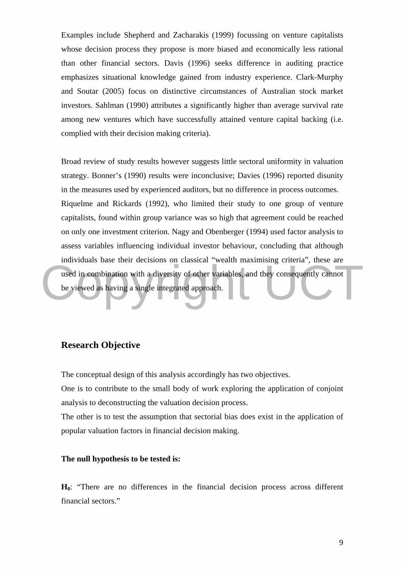
1. Aggregate Data 1.1 Question 1 – Full profile method. Ordinal and Cardinal results. Table 1. Comparison between Cardinal and Ordinal factor ranking.

Factor Levels Ordinal Rank

Ordinal Score

Cardinal Value

Economic Value High/ Low 1 0.131 0.116 Payback Period Short (~2 yrs)/ Long(~ 7 yrs) 2 0.130 0.112 Knowledge of Business New Business/ Franchise 3 0.122 0.111 Market Measures Beta>1/ Beta< 1 4 0.104 0.105 Macroeconomic Factors GDP forecast :Bull/ Bear 5 0.102 0.099 Management Qualification C.A./ Unqualified 6 0.097 0.097 Entry Barriers High/ Low 7 0.078 0.090 Referral Source Personal/ Formal 8 0.078 0.090 Free Cash Flow Good/ Modest 9 0.078 0.090 Price Earnings Ratio Premium/ Discounted 10 0.078 0.090

A Matched pair t-test strongly suggests that the outcomes are identical (p=1). The

range and variance among the cardinal scores is noticeably lower than those of the

ordinal score, suggesting smaller margins of preference between stimuli.

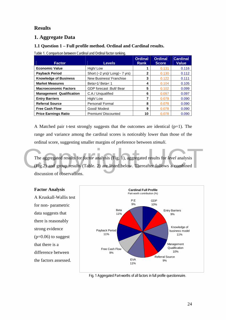
The aggregated results for factor analysis (Fig. 1), aggregated results for level analysis

(Fig.2) and group results (Table. 2) are listed below. Thereafter follows a combined

discussion of observations.

Factor Analysis Cardinal Full ProfilePart-worth contribution (%)

GDP10%

Entry Barriers9%

Knowledge of business model

11%

Management Qualification

10%

Referral Source9%EVA

11%

Free Cash Flow9%

Payback Period11%

Beta11%

P:E9%

A Kruskall-Wallis test

for non- parametric

data suggests that

there is reasonably

strong evidence

(p=0.06) to suggest

that there is a

difference between

the factors assessed.

Fig. 1 Aggregated Part-worths of all factors in full profile questionnaire.

24

Copyright UCT

Level Analysis

Aggregated Part-worth for Full Profile Levels

-1.50 -1.00 -0.50 0.00 0.50 1.00 1.50

GDP Bearish

New Product

Below Ave Economic Value

Moderate F.C.F.

Formal application

Beta<1

Low Entry Barrier

Below Sector P:E

Long Payback

Manager Unqualified

GDP Bullish

Personal Introduction

High F.C.F.

Franchise

High Entry Barrier

Above sector P:E

Beta >1

High Econimic Value

Manager C.A.

Short payback

Fig. 2 Aggregated Part-worths of all levels in full profile questionnaire.

Group Analysis Table 2. Full Profile Factors – Probability of no difference between Groups

Factor Probability Economic Value 0.153

Payback Period 0.690 Knowledge of Business 0.203 Market Measures 0.658 Macroeconomic Factors 0.555 Management Qualification 0.465 Entry Barriers 0.611

Referral Source 0.612 Free Cash Flow 0.610 Price Earnings Ratio 0.612

There were no significant differences between groups for any factor, although

“Economic Value” tends towards significance at a 15% confidence level. Fig. 3 Fisher’s LSD for Full Profile factor Economic Value

Money

Lenders Arms Length

Investors Equity

Investors Prof Advisors Students mean 0.153034 0.127683 0.114226 0.100253 0.091114

25

Copyright UCT

The greatest source of difference between groups points towards Money Lenders

placing higher utility on projects delivering high economic value than do

Professional Advisors and Students respectively.

Discussion

Both ordinal and cardinal scoring systems generate the same preference structure.

While this seems intuitive, there were several respondents who assigned stimuli

different preferences on the two scoring scales. Ordinal scoring forces the respondents

to rank their preferences. Because the increment between ranking positions is constant

at the value of 1, ranking does not capture relative value, and is considered categorical

data. In assigning a cardinal value, the respondent is able to indicate personal utility.

Whereas ranking forces the respondent to choose one product over another, ordinal

scoring permits assigning multiple products the same utility value.

Although the difference between stimuli is highly statistically significant, the

distribution of utility between factors (Fig.1) seems more homogeneous with a 3%

range between the highest and lowest scoring variables. This observation echoes that

of Nagy and Obenberger (1994) who, using factor analysis, found there to be seven

relatively homogeneous groups of variables influencing investor behaviour.

It may be notable that the four lowest scoring factors (Table 1.) all seem to be equally

“thinly traded”. They could possibly be casualties of information overload as the

questionnaire featured the maximum number of ten factors, as opposed to the ideal of

six, as suggested by Hair et al. (1998). This phenomenon is illustrated by Huber,

Wittink, Fielder and Miller (1993), reporting a highly significant (p=0.01) 10% drop

in predictive accuracy when a five attribute full profile questionnaire in expanded to

accommodate nine attributes. Green and Srinivasan (1990) warn that if there is

substantial intercorrelation between factors, it is difficult for the respondent to provide

ratings cet par. This may be the case for Economic Value, Payback Period, Free

Cash Flow and Price Earnings Ratio which, according to Gilbert (2003), are often

used in combination. The former two factors received the highest utility ratings, and

the latter two among the lowest. Conversely, it is equally possible that respondents

did indeed find the former two valuation techniques far more relevant to the presented

stimuli, and the heuristics of the decision process are well reflected.

26

Copyright UCT

Level analysis indicates that most respondents took a “high upside, low down-side”

position, placing the highest utility on quick payback projects and businesses which

are managed by C.A.s. While this may be interpreted as a bias towards liquidity and

conservatism, the next highest levels of worth are those of high EVA and higher

levels of Beta, which may be interpreted as a tempered appetite for risk.

Another consideration in interpreting this result is that the stimuli were generated

through factorial design. Consequently all combinations generated contained some

measure of compromise and no single stimulus offered particularly outstanding

prospects. This preference pattern may thus reflect a “safety first” investor preference

model (Nagy and Obenberger, 1994, 63), concentrating on avoiding “bad outcomes”.

A high level of variance within respondent groups may be a contributor to the lack of

distinction between the groups. The only factor approaching significance was the

appreciation for high economic yield ventures, with the highest utility perhaps

surprisingly lying with the Money Lenders, the least with Professional Advisors and

Students respectively (Fig 3.). While this observation may warrant further

investigation, the overall finding, that the variance within groups is greater than the

difference between groups, does correspond with that of Riquelme and Rickards

(1992) and Nagy and Obenberger (1994).

The factors and levels of the full profile questionnaire are largely self explanatory

(Fig 2.) but where appropriate, are referred to in discussion of the matrix results

below.

27

Copyright UCT

Self Explicating Matrices Question 2.1

Self Explicating Matrix of Management Qualification vs. NOPAT

Aggregated Results.

Management Qualification,

0.34

NOPAT, 0.63

0%

10%

20%

30%

40%

50%

60%

70%

Management Qualification NOPAT

Table 3. Statistic Management Qualification

NOPAT

χ2 test for normality P= 0.128 P=0.07 Bartlett’s Test for Equal Variance P=0.73 Paired T-Test P= 0.001889

Fig4 Aggregated Part-worths Management Qualification Vs. NOPAT

Factor Analysis.

This matrix aims to investigate the extent to which a business’ management’s

qualification may modify business valuation when compared to the traditional

accounting measure of NOPAT. Management qualification and NOPAT are

significantly different factors (P= 0.002), constituting 34% and 63% of the total

decision utility respectively.

Level Analysis

Levels of management qualification are significantly different (p = 1.05 e -16), as are

the three levels of NOPAT (p=0.0) (Appendix 5 – Table 4.)

Part- worths of Management Qualification and NOPAT

y = -0.099x2 + 0.0544x + 0.6064R2 = 0.9983

y = 0.0402x2 - 1.5164x + 2.8451R2 = 1

-1.5

-1

-0.5

0

0.5

1

1.5

2

NonCommercial.

No Qualification

Commercial.C.A.

High NOPAT

Average NOPAT

Low NOPAT

Fig 5. Relative Part- worths for Aggregated levels of Management Qualification and NOPAT.

28

Copyright UCT

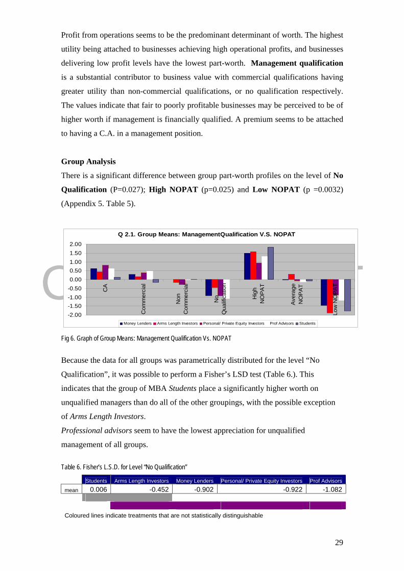
Profit from operations seems to be the predominant determinant of worth. The highest

utility being attached to businesses achieving high operational profits, and businesses

delivering low profit levels have the lowest part-worth. Management qualification

is a substantial contributor to business value with commercial qualifications having

greater utility than non-commercial qualifications, or no qualification respectively.

The values indicate that fair to poorly profitable businesses may be perceived to be of

higher worth if management is financially qualified. A premium seems to be attached

to having a C.A. in a management position.

Group Analysis

There is a significant difference between group part-worth profiles on the level of No

Qualification (P=0.027); High NOPAT (p=0.025) and Low NOPAT (p =0.0032)

(Appendix 5. Table 5).

Q 2.1. Group Means: ManagementQualification V.S. NOPAT

-2.00-1.50-1.00-0.500.000.501.001.502.00

CA

Com

mer

cial

Non

Com

mer

cial

No

Qua

lific

atio

n

Hig

hN

OP

AT

Ave

rage

NO

PA

T

Low

NO

PA

T

Money Lenders Arms Length Investors Personal/ Private Equity Investors Prof Advisors Students Fig 6. Graph of Group Means: Management Qualification Vs. NOPAT

Because the data for all groups was parametrically distributed for the level “No

Qualification”, it was possible to perform a Fisher’s LSD test (Table 6.). This

indicates that the group of MBA Students place a significantly higher worth on

unqualified managers than do all of the other groupings, with the possible exception

of Arms Length Investors.

Professional advisors seem to have the lowest appreciation for unqualified

management of all groups.

Table 6. Fisher’s L.S.D. for Level “No Qualification”

Students Arms Length Investors Money Lenders Personal/ Private Equity Investors Prof Advisors

mean 0.006 -0.452 -0.902 -0.922 -1.082 Coloured lines indicate treatments that are not statistically distinguishable

29

Copyright UCT

Data for both High and Low NOPAT are non-parametric, precluding the use of

Fisher’s LSD test. Possible sources of significant differences (Appendix 5. Table 5.)

are estimated by visual inspection of plots of group mean +/- 1 S.D. (Fig.7 and Fig.8).

Students seem to differ quite starkly form Private Equity Investors, placing the

highest, and lowest utility on High NOPAT levels respectively. Both groups however

find a high measure of worth in this level.

Chart of Mean+/- S.D. for High NOPAT

0.00

0.50

1.00

1.50

2.00

2.50

Money Lenders Arms LengthInv estors

Personal/ Priv ateEquity Inv estors

Prof Adv isors Students

Fig 7. Differences in Group Mean +/- 1 S.D. for Level High NOPAT

A similar pattern seems to hold for the utility of “Low NOPAT”, with a visible

difference between (St) and (PEI) groups, (St) placing a somewhat lower value on low

profit companies. In this case, the (ALI) group also seems to differ from the (PEI)

rating, with a profile which is closer to that of (St).

Chart of Mean+/- S.D. for Low NOPAT

-2.50

-2.00

-1.50

-1.00

-0.50

0.00

0.50

Money Lenders Arms LengthInv estors

Personal/ Priv ateEquity Inv estors

Prof Adv isors Students

Fig 8. Differences in Group Mean +/- 1 S.D. for level Low NOPAT

30

Copyright UCT

Individual Analysis

Individuals who differ significantly from the predictions of this model (Appendix 6.),

seem to do so predominantly in relation two levels. The first is Average NOPAT,

with three respondents finding this level of performance far more agreeable than

most. One advisor differed, rating it far less acceptable than the aggregate.

The second level, Non Commercial Qualification also had three outliers. Two were

professional advisors who respectively found the measure far more and far less

attractive than the aggregate. The third was from the Arms Length Investors group,

and indicated an unusual appreciation for C.A.s, to the detriment of all other included

measures.

Discussion The observations of Fried and Hirsch (1994) and Chemanura and Paeglis (2005)

regarding management qualification are supported by this study. The illustration of

aggregated part-worths (Fig 5.) attests to the elegance of conjoint analysis in

graphically quantifying respondent preferences.

There is perfect correspondence between the matrix and full profile derived

relationships on all levels bar that of the utility of having a C.A. in management. In

the full profile rating, the C.A. scored higher than accounting measures, while in the

matrix, business profitability had the highest utility. This disparity may be due to the

higher risk context provided in the full profile questionnaire, with respondents prizing

the conservative competency of C.A. management.

The high utility allocated to a measure of earnings corresponds with the findings of

Nagy and Obenberger (1994) and Raquelme and Rickards (1992).

The use of multiple levels in the self explicating matrix have permitted the charting of

non-linear relationships for both level series.

The Students’ belief in unqualified management is not unexpected, and possibly

presents a personal bias with a different perspective from that of financial managers.

The response may be explained by Byrne’s (1971) “similarity hypothesis” which

predicts that the higher the similarity between the profile of the assessor to that of the

management team, the more favourable the assessor’s evaluation will be. This

hypothesis would be supported by Franke et al. (2006), who found this to be the case

31

Copyright UCT

among V.C.’s assessing their management teams. Practically, most respondents did

mention that the relevance of qualification depends on the industry, but without

context they offered a generic answer.

On the utility of both high and low NOPAT, the (St) group seems to have differed

most strongly from the (PEI) group. It may be due to the students valuing the business

on current status, while the (PEI) group contained many venture capitalists who seek

businesses as turnaround opportunities.

One of the main purposes of the individual analysis is to identify outliers who have

unusual decision patterns. One Private Equity Investor reported unusually high utility

in high performing companies with non-financial managers. His rationale was that, as

a financial expert, he could purchase a controlling share, and add value in improving

the company’s performance. He did not feel the same opportunities existed when the

company was C.A. managed.

32

Copyright UCT

Question 2.2 Self Explicating Matrix of Entry Barriers vs. Economic Yield (RONA-WACC)

Aggregated Part-worths

42%

58%

0%

10%

20%

30%

40%

50%

60%

70%

Entry Barrier RONA-WACC

Statistic Entry Barrier Yield χ2 test for normality P= 0.109 P=0.109 Bartlett’s Test for Equal Variance P=1 Paired T-Test P= 0.03

Fig. 9 Aggregated Part-worths for Entry Barrier Vs. Economic Yield (PONA-WACC) Factor Analysis

This matrix strives to assess a funder’s appetite for market risk, trading off the

security of high entry barriers against the promise of high economic yield. Entry

barriers and Economic yield are significantly different factors (p=0.03), contributing

42% and 68% of the total decision utility respectively.

Level Analysis

Levels of the factor Entry Barrier were all significantly different (p=0.0), as were

the levels for Economic Yield (p=0.0) (Appendix 7. Table 6)

Part- worths of Entry Barrier and Yield (RONA-WACC)

y = -0.0146x2 - 0.8672x + 1.8026R2 = 1

y = -0.0804x2 - 0.9596x + 2.2942R2 = 1

-1.5

-1

-0.5

0

0.5

1

1.5

High Entry Barrier

Moderate Entry Barrier

Low Entry Barrier

Average Yield

High Yield

Below Average Yield

Fig. 9 Relative Part-worths for Aggregated levels of Entry Barriers and Economic Yield.

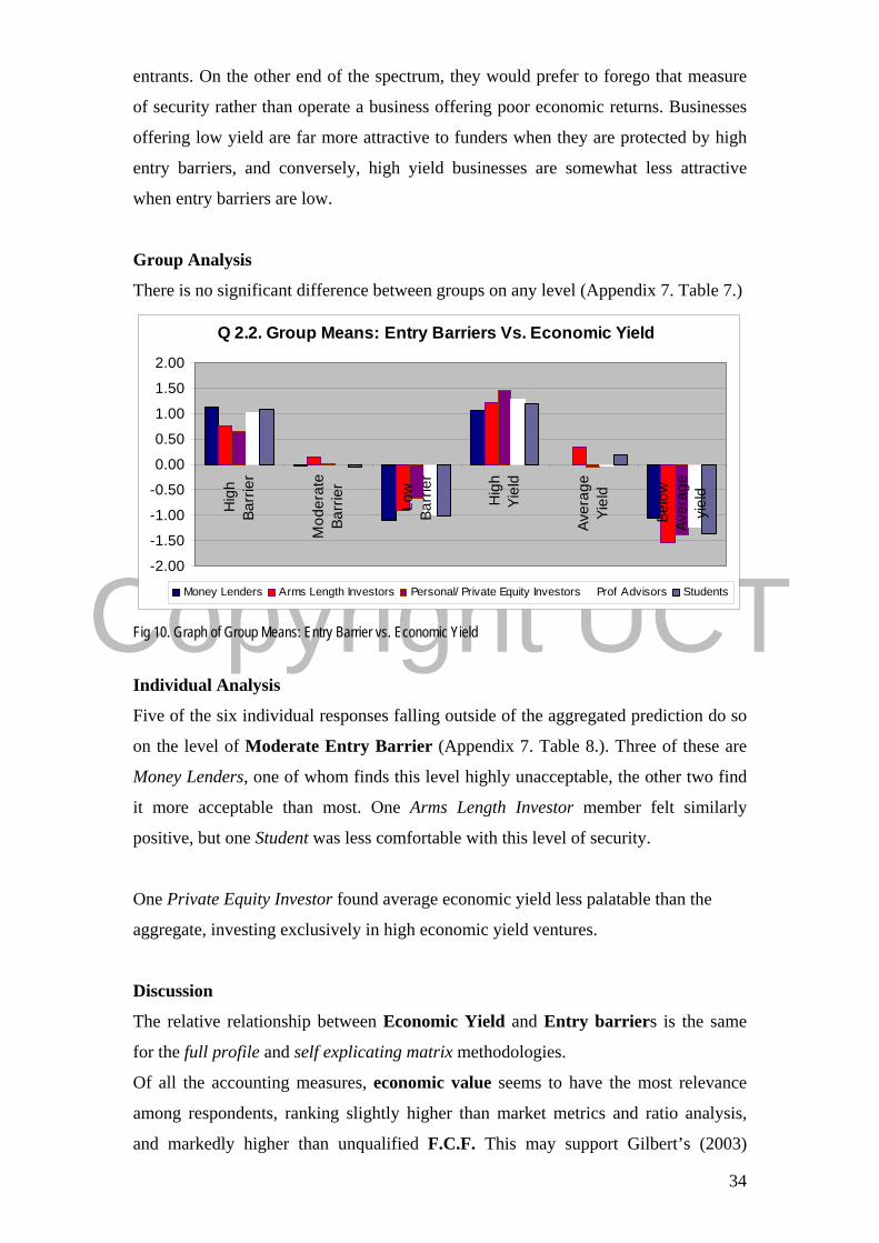
Respondents place the highest utility on businesses offering high economic yield, but

seem similarly appreciative of a high measure of protection against new market

33

Copyright UCT

entrants. On the other end of the spectrum, they would prefer to forego that measure

of security rather than operate a business offering poor economic returns. Businesses

offering low yield are far more attractive to funders when they are protected by high

entry barriers, and conversely, high yield businesses are somewhat less attractive

when entry barriers are low.

Group Analysis

There is no significant difference between groups on any level (Appendix 7. Table 7.)

Q 2.2. Group Means: Entry Barriers Vs. Economic Yield

-2.00

-1.50

-1.00

-0.50

0.00

0.50

1.00

1.50

2.00

Hig

hBa

rrie

r

Mod

erat

eBa

rrie

r

Low

Barr

ier

Hig

hYi

eld

Aver

age

Yiel

d

Belo

wAv

erag

eyi

eld

Money Lenders Arms Length Investors Personal/ Private Equity Investors Prof Advisors Students

Fig 10. Graph of Group Means: Entry Barrier vs. Economic Yield

Individual Analysis

Five of the six individual responses falling outside of the aggregated prediction do so

on the level of Moderate Entry Barrier (Appendix 7. Table 8.). Three of these are

Money Lenders, one of whom finds this level highly unacceptable, the other two find

it more acceptable than most. One Arms Length Investor member felt similarly

positive, but one Student was less comfortable with this level of security.

One Private Equity Investor found average economic yield less palatable than the

aggregate, investing exclusively in high economic yield ventures.

Discussion

The relative relationship between Economic Yield and Entry barriers is the same

for the full profile and self explicating matrix methodologies.

Of all the accounting measures, economic value seems to have the most relevance

among respondents, ranking slightly higher than market metrics and ratio analysis,

and markedly higher than unqualified F.C.F. This may support Gilbert’s (2003)

34

Copyright UCT

findings that a basket of DCF and non DCF measures are used in valuation. This

study’s findings will have to be further qualified, but may point to a different

preference of models between the financial and manufacturing sectors.

Riquelme and Rickards (1992) assertions are similarly supported, although this paper,

in finding no difference between groups, suggests that the values they described are

not unique to venture capitalists alone.

The individual analysis seems to have highlighted some personal idiosyncrasies

reflecting possibly slightly more dogmatic stances among some respondents.

The V.C. characterised as an outlier was identified on the grounds of his extreme bias

towards high yield projects. Of greater interest is his unusual valuation of high and

low entry barriers which were contrary to the norm. His rationale was that high entry

barriers implied more specialised management, thereby exaggerating the information

asymmetry between himself and his staff. Additionally, he felt that lower entry

barriers made the company more tradable, offering him an easier exit strategy.

A similar view was expressed by a business broker.

Neither of these exceptional preference patterns was detected by the statistical tools

employed.

35

Copyright UCT

Question 2.3Question 2.3

Self Explicating Matrix of Information Source vs. P:E ratio Aggregated Results

Information Source,

53% P:E, 44%

0%

10%

20%

30%

40%

50%

60%

Information Source P:E

Statistic Information Source

P:E

χ2 test for normality P= 0.102 P=0.252 Bartlett’s Test for Equal Variance P=0.8828 Paired T-Test P= 0.203

Fig. 11. Aggregated Part-worths for Information Source vs. P:E ratio

Factor Analysis.

This matrix strives to assess preferences in information source when valuing a

company. Positive insights which may be individually derived are compared to

market sentiment as expressed by the prevailing P:E ratio. Results indicate that 53%

of the decision may be influenced by personal insights derived from various

Information Sources, and 44% by the P:E ratio. These weightings are however not

significant (p=0.203).

Level Analysis

There is a significant difference between levels of ‘Information Source’ (p=0.0) and

‘P:E Ratio’ (p=0.0) respectively (Appendix. 8. Table 9.)

Part-worth of P:E Ratio and Information Source

y = 0.175x2 - 1.1958x + 1.5751R2 = 1

y = 0.0486x2 - 1.1453x + 2.0636R2 = 1

-1.50

-1.00

-0.50

0.00

0.50

1.00

1.50

High P:EAve P:E

Low P:E

Management Source

Annual Report

Media Article

Fig. 12. Relative Part-worths for Aggregated levels of Information Source vs. P:E Ratio.

The greatest value is attached to information derived directly form management, with

the least associated with media articles. Funders seek value in low P: E offerings,

seeming reluctant to pay market premiums. Highest utility seems to be associated

36

Copyright UCT

with positive prospects divulged by management of a firm trading at a discount to

sector average. The least utility comes from promising medial articles on already

highly valued stock. Media articles were generally inferred by respondents to indicate

financial publications.

Group Analysis

Q 2.3. Group Means: Information source V.S. P:E ratio

-2.00

-1.50

-1.00

-0.50

0.00

0.50

1.00

1.50

Man

agem

ent

Ann

ual

Rep

ort

Med

ial

Arti

cle

Low

P:E

Ave

rage

P:E

Hig

h P

:E

Money Lenders Arms Length Investors Personal/ Private Equity Investors Prof Advisors Students

Fig 13. Graph of Group Means: Information Source vs. P:E Ratio.

No significant difference was found between groups on any level of analysis

(Appendix 8. Table10.)

Individual Analysis

Nineteen of the twenty individuals falling outside of the predictive model did so on

the relative value attached to information in the Annual Report (Appendix 9, Table

11.) One Professional Advisor was guided exclusively by market measures, and one

student displays far higher than average levels of faith in the media, possibly

distrusting management’s claims.

Discussion

These results are not comparable between the two methodologies used, but the results

obtained do concur with Clark-Murphy and Soutar’s (2005) observations of V.C.’s

and Nagy and Obenberger’s (1994) observations of stock market investors. Again, the

inability of this study to demonstrate a difference between groups may indicate that

these factors are ubiquitously considered in business valuation across sectors.

The large number of outliers on the level of information gleaned from the annual

report is likely to reflect a) the faith placed in the audited report by many who do not

37

Copyright UCT

have access to senior management or b) the feeling that the information offered is

already stale, public domain, and probably sanitized. The latter sentiment was

successfully identified in the X2 test whereby the second highest deviation belonged

to a leading equity fund manager who showed no faith in either management or

annual report, but was guided most strongly by media articles. He does not limit

himself to the formal financial press, and looks for breaking news in all media.

38

Copyright UCT

Question 2.4

Self Explicating Matrix of Marke

g 14 Aggregated Part-worths for Market

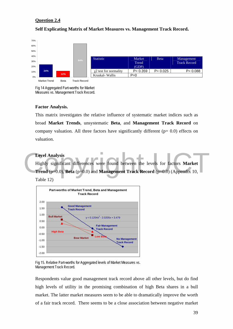
actor Analysis.

igates the relative influence of systematic market indices such as

evel Analysis

nt differences were found between the levels for factors Market

t Measures vs. Management Track Record.

FiMeasures vs. Management Track Record. F

This matrix invest

broad Market Trends, unsystematic Beta, and Management Track Record on

company valuation. All three factors have significantly different (p= 0.0) effects on

valuation.

L

Highly significa

Trend (p=0.0), Beta (p=0.0) and Management Track Record (p=0.0) (Appendix 10,

Table 12)

Part-worths of Market Trend, Beta and Management Track Record

y = 0.1204x2 - 2.0205x + 3.479

-2.00

-1.50

-1.00

-0.50

0.00

0.50

1.00

1.50

2.00Good Management Track Record

Fair Management Track Record

No Management Track Record

Bear Market

Bull Market

High Beta

Low Beta

Fig 15. Relative Part-worths for Aggregated levels of Market Measures vs. Management Track Record.

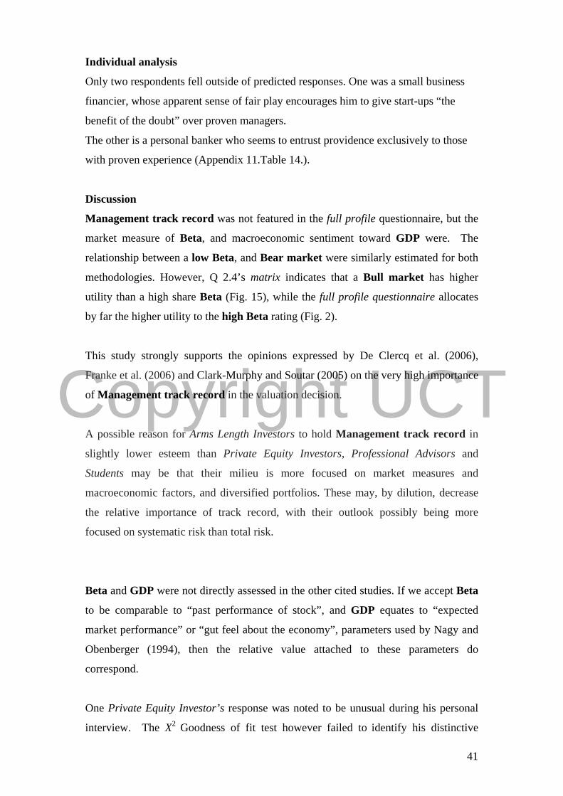
od management track record above all other levels, but do find

Respondents value go

high levels of utility in the promising combination of high Beta shares in a bull

market. The latter market measures seem to be able to dramatically improve the worth

of a fair track record. There seems to be a close association between negative market

Statistic Market Trend (GDP)

Beta Management Track Record

χ2 test for normality P= 0.359 P= 0.025 P= 0.088 Kruskal- Wallis P=0

64%

12%24%

0%

10%

20%

30%

40%

50%

60%

70%

Market Trend Beta Track Record

39

Copyright UCT

predictors and a fair track record, suggesting that valuers of such companies have

little faith in management’s ability to out-perform market troughs. The least value is

placed on companies where management’s record is not known, and enthusiasm for

such entities is even more circumspect than might be expected for foreboding market

forecasts.

Group Analysis

ant difference between groups on the level of Good Track Record There is a signific

(p= 0.045) (Appendix 10, Table 13)

Q 2.4. Group Means: Market Measures V.S. Management Track Record

-2.00

-1.50

-1.00

-0.50

0.00

0.50

1.00

1.50

2.00

Bul

lM

arke

t

Bea

rM

arke

t

Hig

hB

eta

Low

Bet

a

Goo

dTr

ack

Fair

Trac

k

No

Trac

k

Money Lenders Arms Length Investors Personal/ Private Equity Investors Prof Advisors Students

Fig. 16. Graph of Group Means: Market Measures vs. Management Track Record.

raphic inspection suggests a likely difference between Arms Length Investors, who

G

place relatively lower value on good track record , and Private Equity Investors,

Professional Advisors and Students who hold the parameter in increasing regard

respectively.

Chart of Mean+/- S.D. for Good Track Record

-0.50

0.00

0.50

1.00

1.50

2.00

2.50

Money Lenders Arms Length Investors Personal/ PrivateEquity Investors

Prof Adv isors Students

Fig 16. Differences in Group Mean +/- 1 S.D. for level Good Track Record.

40

Copyright UCT

Individual analysis

Only two respondents fell outside of predicted responses. One was a small business

financier, whose apparent sense of fair play encourages him to give start-ups “the

benefit of the doubt” over proven managers.

The other is a personal banker who seems to entrust providence exclusively to those

with proven experience (Appendix 11.Table 14.).

Discussion

Management track record was not featured in the full profile questionnaire, but the

market measure of Beta, and macroeconomic sentiment toward GDP were. The

relationship between a low Beta, and Bear market were similarly estimated for both

methodologies. However, Q 2.4’s matrix indicates that a Bull market has higher

utility than a high share Beta (Fig. 15), while the full profile questionnaire allocates

by far the higher utility to the high Beta rating (Fig. 2).

This study strongly supports the opinions expressed by De Clercq et al. (2006),

Franke et al. (2006) and Clark-Murphy and Soutar (2005) on the very high importance

of Management track record in the valuation decision.

A possible reason for Arms Length Investors to hold Management track record in

slightly lower esteem than Private Equity Investors, Professional Advisors and

Students may be that their milieu is more focused on market measures and

macroeconomic factors, and diversified portfolios. These may, by dilution, decrease

the relative importance of track record, with their outlook possibly being more

focused on systematic risk than total risk.

Beta and GDP were not directly assessed in the other cited studies. If we accept Beta

to be comparable to “past performance of stock”, and GDP equates to “expected

market performance” or “gut feel about the economy”, parameters used by Nagy and

Obenberger (1994), then the relative value attached to these parameters do

correspond.

One Private Equity Investor’s response was noted to be unusual during his personal

interview. The X2 Goodness of fit test however failed to identify his distinctive

41

Copyright UCT

valuation criteria. He placed highest value on companies with high Betas in a bear

market, but with a good management track record. His rationale was that in a bull

market, all funds perform well, and there is little to distinguish between them. When

the markets turn, however, disgruntled investors shop around for better yields. He

specifically seeks companies which perform well in that environment, aiming to pick

up new clients during economic downturn. They are then easy to retain when the

markets improve. He thus grows his client base with each successive negative

economic cycle.

42

Copyright UCT

Question 2.5

Self Explicating Matrix of Economic Value Added vs. Payback Period.

Fig. 17. Aggregated Part-worths for EVA Vs. Payback Period

Factor Analysis

EVA and Payback period are both measures used in valuing prospective ventures. The

EVA measure is not time sensitive, and conversely, prizing fast payback may be at the

expense of more profitable opportunities which have a longer period to maturity. This

matrix explores investor preference between these considerations. The data indicate

that EVA accounts for 53% of the valuation consideration, and Payback period 47%.

There is however no statistically significant distinction between the two factors

(p= 0.31).

Level Analysis

Highly significant differences were found between all levels of EVA (P=0.0) and

Payback Period (p= 0.0) (Appendix 12, Table 15).

Part-worths of EVA and Payback Period

y = -0.0607x2 - 0.8018x + 1.8869R2 = 1

y = 0.0231x2 - 1.2694x + 2.4311R2 = 1

-1.50

-1.00

-0.50

0.00

0.50

1.00

1.50

<2yr payback

2-6yr payback

>6yr payback

High EVA

Low EVA

Moderate EVA

Fig 18. Relative Part-worths for Aggregated levels of EVA and Payback Period.

Respondents have placed similarly high value on short payback and high EVA

prospects. They have an accordingly poor appetite for ventures offering low economic

returns, or offering payback after a period longer than six years. Low, but positive

Statistic EVA Payback

χ2 test for normality p=0.22 p=0.22 Bartlett’s Test for Equal Variance Paired T-Test p=0.31

47%53%

40%

45%

50%

55%

EVA Payback Period

43

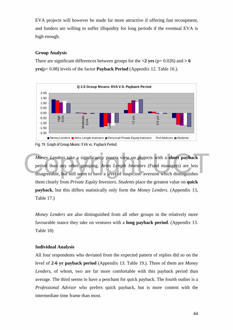
Copyright UCT

EVA projects will however be made far more attractive if offering fast recoupment,

and funders are willing to suffer illiquidity for long periods if the eventual EVA is

high enough.

Group Analysis

There are significant differences between groups for the <2 yrs (p= 0.026) and > 6

yrs(p= 0.08) levels of the factor Payback Period (Appendix 12. Table 16.).

Q 2.5 Group Means: EVA V.S. Payback Period

-2.00-1.50-1.00-0.500.000.501.001.502.00

Hig

hE

VA

Mod

erat

eE

VA

Low

EV

A

<2 y

rs

2-6

yrs

>6yr

s

Money Lenders Arms Length Investors Personal/ Private Equity Investors Prof Advisors Students

Fig. 19 Graph of Group Means: EVA vs. Payback Period.

Money Lenders take a significantly poorer view on projects with a short payback

period than any other grouping. Arms Length Investors (Fund managers) are less

disagreeable, but still seem to have a level of suspicion/ aversion which distinguishes

them clearly from Private Equity Investors. Students place the greatest value on quick

payback, but this differs statistically only form the Money Lenders. (Appendix 13,

Table 17.)

Money Lenders are also distinguished from all other groups in the relatively more

favourable stance they take on ventures with a long payback period. (Appendix 13.

Table 18)

Individual Analysis

All four respondents who deviated from the expected pattern of replies did so on the

level of 2-6 yr payback period (Appendix 13. Table 19.). Three of them are Money

Lenders, of whom, two are far more comfortable with this payback period than

average. The third seems to have a penchant for quick payback. The fourth outlier is a

Professional Advisor who prefers quick payback, but is more content with the

intermediate time frame than most.

44

Copyright UCT

Two Money Lenders had significantly stronger views on Moderate EVA than

average. One was more favourable, one less.

Discussion

These results seem to support the findings of Grinyer and Green (2003), who claim

that under simulated “normal” conditions, the use of payback period would yield

much the same result as a more complex DCF calculation such as Economic Yield.

It is reported by Correia, Flynn, Uliana and Wormald (2003) that the two

methodologies are commonly used in combination with each other, or with additional

measures as appropriate.

In this study the outcomes of both measures were provided, and the respondent did

not have to consider the implications of performing the calculations. Determinants of

the better choice of measure may include availability of information, time constraints,

valuation costs, and the magnitude of the financial decision being made. Without

these considerations it is perhaps not unexpected that no clear preference between

methodology is made.

Moneylenders’ less favourable view on short payback, and more favourable position

on long payback probably reflects their bias towards longer term loans. One financier

said that he felt that a venture offering quick payback inherently held higher risk. He

asserted that he was not swayed by the length of the payback period, he just adjusted

the risk premium accordingly. By contrast, another explained that he preferred high

economic yield ventures with a longer payback period as these served to smooth his

income streams should the markets experience turbulence.

45

Copyright UCT

Question 2.6 Self Explicating Matrix of Competitive Risk vs. Internal Risk

53%

47%

42%

44%

46%

48%

50%

52%

54%

Ext Comp Internal Risk

Statistic External Comp

Intrinsic risk

χ2 test for normality p=0.37 p=0.37 Bartlett’s Test for Equal Variance p=1.00 Paired T-Test p=0.20

Fig. 20 Aggregated Part-worths for External Competition vs. Intrinsic Risk

Factor Analysis.

This matrix attempts to explore the valuers’ preference /aversion towards external

risks stemming from the nature of the industry under consideration, as opposed to

benefits or liabilities associated with the extent of knowledge of the business’

operations. The data indicate that 53% of consideration will revolve around external

factors, and 47% around understanding of the business model. There is however no

statistical difference in this weighting (p= 0.20).

Level Analysis

There is a significant difference between all levels assessed for External Competition (p=0.0) and Internal Risk (p=0.0) respectively (Appendix 14. Table 20.)

Part-worths of External Competition and Internal Risk

y = -0.1155x2 - 0.5457x + 1.6304R2 = 1

y = -0.3851x2 + 0.3777x + 1.0419R2 = 1

-1.50

-1.00

-0.50

0.00

0.50

1.00

1.50

Collabourative Competition

Cooperative Competition Fierce

Competition

Own Niche Market

Franchise/ Known Model

New Business Model

Fig. 21 Relative Part-worths for aggregated levels of External Risk and Internal Competition.

46

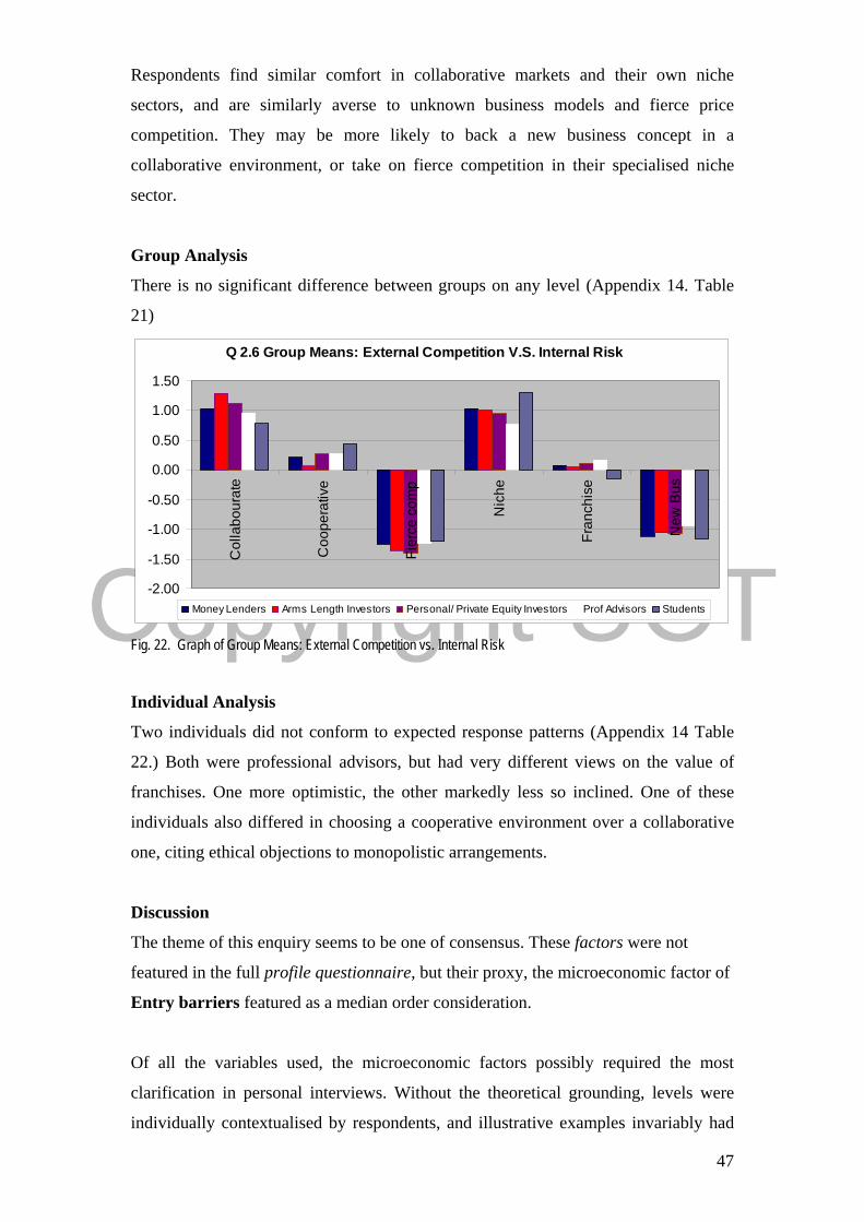
Copyright UCT

Respondents find similar comfort in collaborative markets and their own niche

sectors, and are similarly averse to unknown business models and fierce price

competition. They may be more likely to back a new business concept in a

collaborative environment, or take on fierce competition in their specialised niche

sector.

Group Analysis

There is no significant difference between groups on any level (Appendix 14. Table

21)

Q 2.6 Group Means: External Competition V.S. Internal Risk

-2.00

-1.50

-1.00

-0.50

0.00

0.50

1.00

1.50

Col

labo

urat

e

Coo

pera

tive

Fier

ce c

omp

Nic

he

Fran

chis

e

New

Bus

Money Lenders Arms Length Investors Personal/ Private Equity Investors Prof Advisors Students

Fig. 22. Graph of Group Means: External Competition vs. Internal Risk

Individual Analysis

Two individuals did not conform to expected response patterns (Appendix 14 Table

22.) Both were professional advisors, but had very different views on the value of

franchises. One more optimistic, the other markedly less so inclined. One of these

individuals also differed in choosing a cooperative environment over a collaborative

one, citing ethical objections to monopolistic arrangements.

Discussion

The theme of this enquiry seems to be one of consensus. These factors were not

featured in the full profile questionnaire, but their proxy, the microeconomic factor of

Entry barriers featured as a median order consideration.

Of all the variables used, the microeconomic factors possibly required the most

clarification in personal interviews. Without the theoretical grounding, levels were

individually contextualised by respondents, and illustrative examples invariably had

47

Copyright UCT

implications beyond the intention of the study. Examples include the use of pharmacy

and authorised financial services to illustrate higher entry barrier industries. Both

sectors were however experiencing some distress at the time of this study, and may

have been interpreted with unanticipated inferences. Collaborative and cooperative

competition were concepts which clearly eluded some respondents, who interpreted

them to indicate monopolies or oligarchies.

Utility ratings for comparable microeconomic factors were not performed in the cited

references, leaving no basis of comparison for this study’s results. Despite the

complexities around these factors, there is no reason to suspect that they have not

been allocated their appropriate part-worth scores.

48

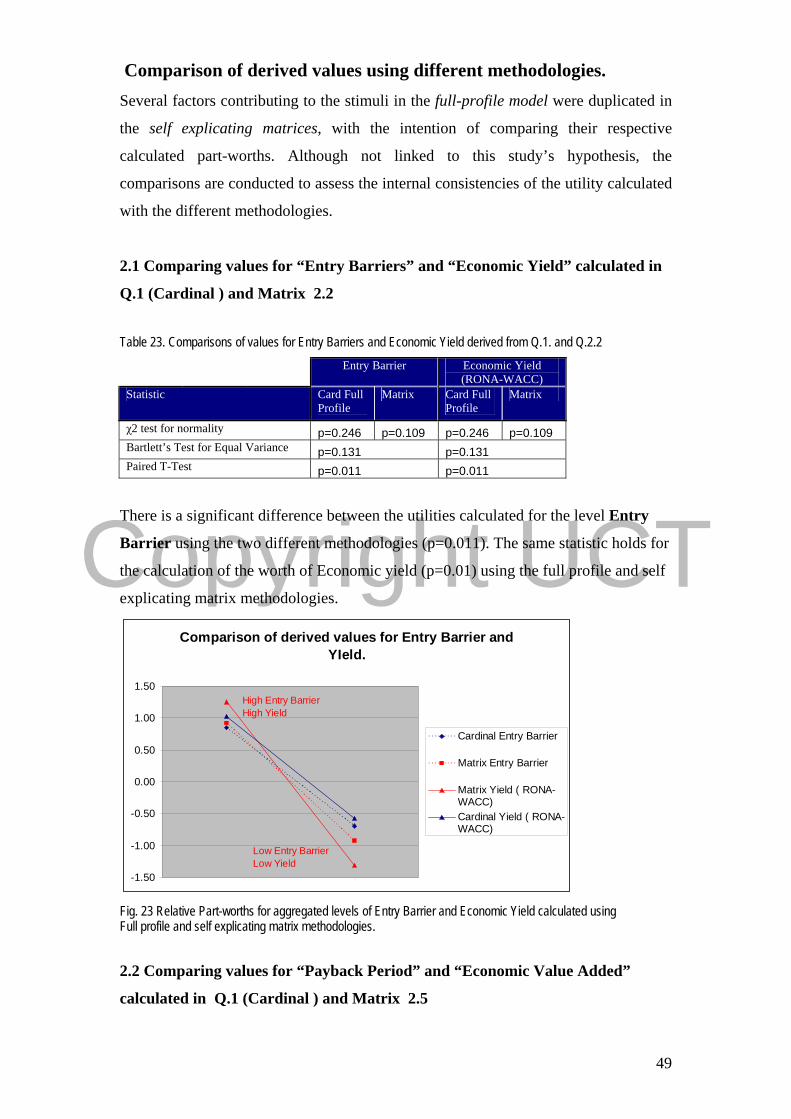
Copyright UCT

Comparison of derived values using different methodologies. Several factors contributing to the stimuli in the full-profile model were duplicated in

the self explicating matrices, with the intention of comparing their respective

calculated part-worths. Although not linked to this study’s hypothesis, the

comparisons are conducted to assess the internal consistencies of the utility calculated

with the different methodologies.

2.1 Comparing values for “Entry Barriers” and “Economic Yield” calculated in

Q.1 (Cardinal ) and Matrix 2.2 Table 23. Comparisons of values for Entry Barriers and Economic Yield derived from Q.1. and Q.2.2

Entry Barrier Economic Yield (RONA-WACC)

Statistic Card Full Profile

Matrix Card Full Profile

Matrix

χ2 test for normality p=0.246 p=0.109 p=0.246 p=0.109 Bartlett’s Test for Equal Variance p=0.131 p=0.131 Paired T-Test p=0.011 p=0.011

There is a significant difference between the utilities calculated for the level Entry

Barrier using the two different methodologies (p=0.011). The same statistic holds for

the calculation of the worth of Economic yield (p=0.01) using the full profile and self

explicating matrix methodologies.

Comparison of derived values for Entry Barrier and YIeld.

-1.50

-1.00

-0.50

0.00

0.50

1.00

1.50

Cardinal Entry Barrier

Matrix Entry Barrier

Matrix Yield ( RONA-WACC)Cardinal Yield ( RONA-WACC)

High Entry BarrierHigh Yield

Low Entry BarrierLow Yield

Fig. 23 Relative Part-worths for aggregated levels of Entry Barrier and Economic Yield calculated using Full profile and self explicating matrix methodologies.

2.2 Comparing values for “Payback Period” and “Economic Value Added”

calculated in Q.1 (Cardinal ) and Matrix 2.5

49

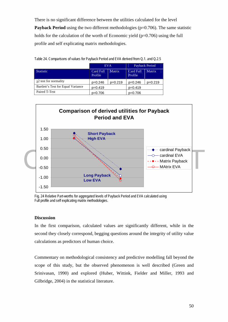
Copyright UCT

There is no significant difference between the utilities calculated for the level

Payback Period using the two different methodologies (p=0.706). The same statistic

holds for the calculation of the worth of Economic yield (p=0.706) using the full

profile and self explicating matrix methodologies.

Table 24. Comparisons of values for Payback Period and EVA derived from Q.1. and Q.2.5

EVA Payback Period

Statistic Card Full Profile

Matrix Card Full Profile

Matrix

χ2 test for normality p=0.246 p=0.219 p=0.246 p=0.219 Bartlett’s Test for Equal Variance p=0.419 p=0.419 Paired T-Test p=0.706 p=0.706

Comparison of derived utilities for Payback Period and EVA

-1.50

-1.00

-0.50

0.00

0.50

1.00

1.50

cardinal Paybackcardinal EVAMatrix PaybackMAtrix EVA

Short PaybackHigh EVA

Long PaybackLow EVA

Fig. 24 Relative Part-worths for aggregated levels of Payback Period and EVA calculated using Full profile and self explicating matrix methodologies.

Discussion

In the first comparison, calculated values are significantly different, while in the

second they closely correspond, begging questions around the integrity of utility value

calculations as predictors of human choice.

Commentary on methodological consistency and predictive modelling fall beyond the

scope of this study, but the observed phenomenon is well described (Green and

Srinivasan, 1990) and explored (Huber, Wittink, Fielder and Miller, 1993 and

Gilbridge, 2004) in the statistical literature.

50

Copyright UCT

In brief summary, Huber et al. (1993) find that the choice process is a maze of

heuristics, and any combination of methods included in an adaptive design will be

better than any method alone. The self explicating matrices are not a stand alone

methodology, and although easy to design and administer, run the risk of focusing

inordinate time and attention on less important attributes.

In this study it was felt that in introducing the matrix first, the respondent may

formulate some heuristic which would be applied to the full profile method, possibly

modifying the respondent’s decision paradigm. The full profile method was therefore

applied first. Huber et al. (1993) report that presenting the self explicating method

before the full profile method leads to a higher measure of consistency than the

reverse order. However, in applying the full profile first, predictions are more

accurate. His first observation may help to explain the inconsistency observed, and the

second to justify the rationale applied.

The combined result of the full profile and self explicating matrices should offer the

best predictive model. The final utility for each level may be determined using logit

methodology or specific axioms (Gilbridge, 2004), which fall beyond the

methodology used in this study. Since the full profile method permits the assessment

of a far greater number of levels, and better real life simulation, a practical solution

may be to average the part-worths of calculated levels, with a weighting bias in favour

of the full profile results.

51

Copyright UCT

Conclusions This study’s first objective is to contribute to the small body of work exploring the

application of conjoint analysis to deconstructing the valuation decision process.

Results suggest that that the type and quality of the data derived is consistent with that

reported in the literature, and that the models used are methodologically comparable.

The data generated seem empirically definitive, and proved useful and unambiguous

in interpretation. These factors may suggest that the study conforms to conjoint

requirements, and motivates for the use of this methodology in future valuation

decision elucidating research.

The second objective is to test the assumption that sectoral bias does exist in the

application of popular valuation factors in financial decision making, the stated

hypotheses being:

H0: “There are no differences in the financial decision process across different

financial sectors.”

H1: “There are differences in the financial decision process across different financial

sectors.”

To this end, numerous factors and levels were developed, and subjected to rigorous

statistical validation on an aggregated level before scrutinizing them for difference

between groups.

The findings of the various investigations are summarized in Table 25. below.

Table 25. Summary Table of Levels which indicated between group differences Question

Q1.1 GDP Bearish New Product

Below Ave Economic Value

Moderate F.C.F.

Formal application Beta<1

Low Entry Barrier

Below Sector P:E Long Payback

Manager Unqualified

Q1.1 (ctd) GDP BullishPersonal Introduction High F.C.F. Franchise

High Entry Barrier

Above sector P:E Beta >1

High Econimic Value Manager C.A.

Short payback

Q 2.1 CA CommercialNon

CommercialNo

Qualification High NOPATAverage NOPAT Low NOPAT

Q2.2High Entry

BarrierModerate

Entry BarrierLow Entry

Barrier High Yield Average YieldBelow Ave

Yld Legend

Q2.3 ManagementAnnual Report Medial Article Low P:E Average P:E High P:E p<0.05

Q2.4 Bull Market Bear Market High Beta Low Beta Good Track Fair Track No Track p<0.10

Q2.5 High EVAModerate

EVA Low EVA <2 yr Payback2-6 yr

Payback >6 yr PaybackQ2.6 Collaborate Cooperative Fierce comp Niche Franchise New Bus

Levels indicating between group differences

Significant differences were not ubiquitous, and sometimes may seem more

idiosyncratic than substantive. However for six of the fifty eight levels assessed,

52

Copyright UCT

significant differences between groups were found. The null hypothesis is therefore

rejected, thereby concluding that there is evidence supporting the hypothesis that

“There are differences in the financial decision process across different financial

sectors”.

Future Research

In reviewing the possible contribution of this study to future research, each of the

identified inter-group differences may warrant further investigation. Of specific

interest may be the suggestion of Q.1. that bankers and small business financiers seem

to place a higher value on economic yield than do personal advisors; and the findings

of Q.2.1 that investors may be biased against entrepreneurs with non-financial or no

qualifications. If the latter proves to be the case and it is explained by the “similarity

hypothesis”, then such business propositions, having been previously overlooked,

may prove to be an under exploited source of investment opportunity.

Outside of the group analysis, individual outliers may be representative of an

important albeit less common sentiment. One example is the leading fund manager

who relies disproportionately on lay press for investment guidance. An interesting

study may be the effect of lay press on share price.

On a more empirical level, this study does draw attention to the difference between

individual bias and sectoral bias, implicitly questioning the premise of similar

research which has been narrowly focused on one sector. That is not to criticize the

other study designs, but to consider that if as much of the insight is derived from the

individual as from the sector, then there may be value in having a common module to

future conjoint studies which can transcend sector specificity. As mentioned, one of

the limitations of conjoint analysis is the restricted number of factors which may be

included. Those currently used are not ubiquitous, limiting the correlations which can

be drawn between studies. A common scale of measurement may resemble the

psychometric instruments already used to assess attitudes towards financial risk

(Grable and Lyttleton, 1999).

A corollary to the observation that there are relatively few differences between bias

derived from the financial sector, is the possibility that the bias is a function of the

asset, and not the financial sector being reviewed. By way of illustration, the same

individuals using a specific set of valuation instruments in one sector are likely to use

53

Copyright UCT

a different set of methodologies as appropriate to value a different asset. In attempting

to accommodate a diversity of sectors in this study, the stimuli developed were

deliberately generic. Future studies may include far more focused stimuli, specific to

one asset class, and applied to respondents from different sectors. These may reveal

more acute differences in terms of perceptions of risk and weighting of factors. If

these were presented as an adaptive conjoint in combination with a validated

preference scale, results could contribute more asset specific insight and

simultaneously more cohesive body of work.

54

Copyright UCT

Appendix 1.

Conjoint Attributes and Decision Scenarios.

CodingParameters Factors Levels Field A E F G H J

1

B C D I K1 GDP Bullish ME1 1 1 0 1 1 1 1 62 GDP Bearish ME2 1 1 1 1 1 53 Entry Barrier High PE1 1 1 1 1 1 54 Entry Barrier Low PE3 1 1 1 1 1 1 65 Investor Focus Franchise NC1 1 1 1 1 1 1 66 Investor Focus New Product NC2 1 1 1 1 1 57 Qualification Financial MQ1 1 1 1 1 58 Qualification None MQ3 1 1 1 1 1 1 69 Introduction Personal MS1 1 1 1 1 1 1 6

10 Introduction Formal Channel MS2 1 1 1 1 1 511 RONA - WACC High VR1 1 1 1 1 1 0 1 612 RONA - WACC Below Ave VR3 1 1 1 1 1 513 Free Cash Flow HIgh VB1 1 1 1 1 1 1 614 Free Cash Flow Mod VB2 1 1 1 1 1 515 Payback Short VN1 1 1 1 1 1 516 Payback Long VN2 1 1 1 1 1 1 617 beta ~ 1 VP1 1 1 1 1 1 1 618 beta between 0 and 1 VP3 1 1 1 0 1 1 519 P.E. Above Sector VPE1 1 1 1 1 1 520 P:E Below Sector VPE3 1 1 1 1 1 1 6

Sum of Levels 9 9 9 9 9 9 9 9 9 9 9

Note - Options E, F& J are identical to A, except fot the red, highlighted factor

Valuation Ratio

Management Team

Referral Source

Valuation DCF

Valuation DCF

Valuation DCF

Valuation Ratio

Micro-economic

Niche Focus

Macro-economic

TREATMENTS

55

Copyright UCT

Appendix 2. Test: Assume that you are a financier faced with 5 the following funding opportunities.

a) Please familiarize yourself with each, and rank the in order of preference (1 = first option, 5 = last option.)

b) Assign each option a mark out of 10. (10 = brilliant, 0 = dead in the water)

A Rank (1-5) Mark / 10

A trusted colleague introduces you to a young entrepreneur seeking finance to purchase a franchised coffee shop. Being a cash business, the model features high levels of free cash flow (F.C.F). Economic Value (RONA- WACC) is also high. The entrepreneur has no formal qualification, and the cost of the franchise necessitated a long payback period of 7 years. The shop has a Beta of 1.2, and trades off a P:E ratio with is below the comparable market average. Economic prospects for the forecast period are good with a high expected GDP.

B Rank (1-5) Mark / 10

You receive a formal application for finance from a C.A. looking to purchase a pharmacy in a franchised chain. Competing bids for the pharmacy have set the price at a P:E level which is above the sector average. It has a calculated Beta of 1.1. The business does trade off a book, and free cash flow (F.C.F.) is moderate. Calculation of economic value (RONA –WACC) is high, and the payback period is a projected 2.5 years. Economic forecasts expect a drop in GDP.

C Rank (1-5) Mark / 10

You receive a formal application from an unskilled entrepreneur who has been assisted by consultants in drawing up his proposal. He has designed a new product which has been patented, and wants to manufacture through an engineering company. Projections seem realistic, economic value (RONA-WACC) is low. Free cash flow is modest, and the payback period is seven years. However other respected investors have bought in at a higher than average P:E ratio, and a projected Beta is 1.4. Economic forecasts are positive, expecting an increase in GDP.

D Rank (1-5) Mark / 10

A business associate recommends you to an entrepreneur who has no formal qualification, but wishes to invest in a new and novel car wash operation. Being a cash business, FCF projections are very good, although economic value (RONA-WACC) is slightly lower than for comparable businesses. The investment payback period is within 2 years, and the entrepreneur is offering an equity share at a below average P:E ratio. A projected Beta is ~1. The GDP economic forecast is a little bearish.

E A trusted colleague introduces you to a young entrepreneur seeking finance to purchase a franchised pizza shop. Being a cash business, the model features high levels of free cash flow. The entrepreneur has no formal qualification, and the cost of the franchise necessitated a long payback period of 7 years. The franchise food sector has a high Beta of 1.1. This shop is on for sale at a P:E ratio with is below the market average. Calculated economic value(RONA- WACC) is however high. Economic prospects for the forecast period are gloomy with a drop expected in GDP.

56

Copyright UCT

Appendix 2. (Ctd) Test: Assume that you are a financier faced with 5 the following funding opportunities.

c) Please familiarize yourself with each, and rank the in order of preference (1 = first option, 5 = last option.)

d) Assign each option a mark out of 10. (10 = brilliant, 0 = dead in the water)

F Rank (1-5) Mark / 10

A trusted colleague introduces you to a young entrepreneur seeking finance to purchase a franchised coffee shop. Being a cash business, the model features high levels of free cash flow, and calculated economic value (RONA- WACC) is high. The entrepreneur has no formal qualification, and the cost of the franchise necessitated a seven year payback period. The boutique coffee shop sector trades at a calculated Beta of 1.01. This outlet is priced at a P:E ratio with is below the sector average. Economic prospects for the forecast period are good with a high expected GDP.

G Rank (1-5) Mark / 10

You receive a formal application for finance from a C.A. looking to open a new financial services brokerage in an un-serviced market. Current investors have bought in at a P:E which is above the sector average. The venture has an estimated Beta of 0.6. The business will trade off debit orders, and F.C.F. is initially expected to be moderate. Calculated economic value(RONA –WACC) is below market average, but the industry is not capital intensive, and payback is expected within 3 years. Economic forecasts predict a drop in GDP.

H Rank (1-5) Mark / 10

You receive a formal application from a D.I.Y. enthusiast, who has designed a new home security device which has been patented, and which he wants to manufacture through an electronics company. Projections seem realistic, free cash flow (FCF) is modest, economic value (RONA-WACC) is a little below average, and the payback period is seven years. However other respected investors have bought in at a higher than average P:E ratio. A reliably projected Beta is 1.01. Economic forecasts are positive, expecting an increase in GDP.

I Rank (1-5) Mark / 10

A trusted business associate recommends you to a C.A. who seeks capital to invest in a new and novel corporate events management operation. With low fixed overheads, Free cash flow (FCF) projections are very good, although economic value(RONA-WACC) is slightly lower than for comparable businesses. The investment payback period is within 2 years, and the entrepreneur is offering an equity share at a below average P:E ratio. A projected Beta is ~1. Economic outlook is a little bearish, expecting a drop in GDP.

J Rank (1-5) Mark / 10

A close friend introduces you to a young entrepreneur seeking finance to purchase a franchised video shop. Being a cash business, the model features high levels of free cash flow. The entrepreneur has no formal qualification, and the cost of the franchise necessitated a long payback period of 7 years. Calculated economic value (RONA- WACC) is moderate. The franchise has a Beta of 0.5, and outlets price suggests a P:E ratio with is below the sector average. Economic prospects for the forecast period promise an increase in GDP.

57

Copyright UCT

Appendix 3

Question 2 In valuing a business venture, what relative score would you allocate to the following combinationsof attributes?

Example Shop position Vs. Product demand

Prime 10 7 *

Poor 4 * 0*

* your personal relative value

58

High Low

1 Qualification VS.NOPAT

C.A. 10

Commercial

Non Commercial

NoneHigh Average Low

2 Entry Barrier V.S.(RoNA-WACC)

High 10

ModerateLow

High AverageBelow Average

3 Positive Information Flow VS. P:E. Ratio

Management 10

Annual Report

Media Article

Low Average High

4 Market Measures VS. Management Track RecordHigh Beta Bull market 101>Beta >0 Bull market1>Beta >0 Bear marketHigh Beta Bear market

Good Fair None

5 Economic Value VS. Payback Period

High 10

Moderate

Low

<2 years 2 to 6 yrs >6 to 10 yrs

6 Competitive Risk VS. Internal Risk

Collaborative 10

Cooperative

FierceOwn Niche Sector

Franchise/ established model

New Business

Payback Period

Com

petit

ion

Info

rmat

ion

Sour

ce

P:E Ratio (compared to sector average)

EVA

Familiarity

Track Record

Posi

tion

Product Demand

Mea

sure

sQ

ualif

icat

ion

NOPAT

Entr

y B

arrie

rs

(RONA-WACC)

Copyright UCT

Appendix 5

Graphs and Statistics for Q. 2.1 Management Qualification VS. NOPAT

Q2.1 Raw Data of Part-worths: Management Qualification

-3.00

-2.00

-1.00

0.00

1.00

2.00

3.00

w w w w w w x x x x x y y y y y y y y z z z z z z z z z z z zz zz zz zz zz

CA Commercial Non Commercial No Qualification

Q2.1 Raw Data of Part-worths: NOPAT

-2.50-2.00-1.50-1.00-0.500.000.501.001.502.002.50

w w w x x x y y y y z z z z z zz zz zz

High NOPAT Average NOPAT Low NOPAT

Table 4. Level Analysis for Management Qualification vs. NOPAT

Management Qualification NOPAT

Statistic C.A. Commercial Non Commercial

None High Moderate Low

χ2 test for normality P=0.128 P= 0.095 P=0.128 P=0.094

P= 0.007 P= 0.252

P= 0.005

Bartlett’s Test for Equal Variance

P= 0.1388 P= 0.0105

ANOVA/ Kruskal Wallis

P= 1.05E-16 P= 0.0

Table 5. Group Analysis Qualification vs. NOPAT CA

Commercial

Non Commercial

No Qualification

High NOPAT

Average NOPAT

Low NOPAT

Kruskal Wallis/ ANOVA 0.369 0.2797 0.7259 0.027 + 0.0251+ 0.236 0.0032+

+ Significant difference at 5% confidence interval

59

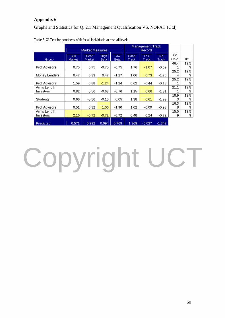
Copyright UCT

Appendix 6

Graphs and Statistics for Q. 2.1 Management Qualification VS. NOPAT (Ctd)

Table 5. X2 Test for goodness of fit for all individuals across all levels.

Market Measures Management Track

Record

Group Bull

Market Bear

Market High Beta

Low Beta

Good Track

Fair Track

No Track

X2 Calc X2

Prof Advisors 0.75 0.75 -0.75 -0.75 1.76 -1.07 -0.69 46.4

1 12.5

9

Money Lenders 0.47 0.33 0.47 -1.27 1.06 0.73 -1.78 25.2

4 12.5

9

Prof Advisors 1.59 0.88 -1.24 -1.24 0.62 -0.44 -0.18 25.2

1 12.5

9 Arms Length Investors 0.82 0.56 -0.63 -0.76 1.15 0.66 -1.81

21.11

12.59

Students 0.66 -0.56 -0.15 0.05 1.38 0.61 -1.99 18.9

3 12.5

9

Prof Advisors 0.51 0.32 1.06 -1.90 1.02 -0.09 -0.93 16.3

8 12.5

9 Arms Length Investors 2.16 -0.72 -0.72 -0.72 0.48 0.24 -0.72

15.59

12.59

Predicted 0.571 0.292 -

0.094 -

0.769 1.369 -0.027 -1.342

60

Copyright UCT

Appendix 7.

Graphs and statistics for Q. 2.2 Entry Barriers vs. Economic Yield (RONA-WACC)

Q2.2 Raw Data of Part-worths: Entry Barriers

-2.50-2.00-1.50-1.00-0.500.000.501.001.502.002.50

w w w x x x y y y y z z z z z zz zz zz

High Entry Barrier Moderate Entry Barrier Low Entry Barrier

Q2.2 Raw Data of Part-worths: Economic Yield

-2.50-2.00-1.50-1.00-0.500.000.501.001.502.002.50

w w w x x x y y y y z z z z z zz zz zz

High Yield Average Yield Below Ave Yield

Table 6. Level Analysis for Entry Barrier vs. Economic Yield (RONA-WACC)

Entry Barrier (RONA-WACC)

Statistic High Moderate Low High Moderate Low χ2 test for normality P= 0.199 P=0.084 P= 0.652 P= 0.003 P= 0.156 P= 0.211 Bartlett’s Test for Equal Variance P= 0.0 Kruskal- Wallis P= 0.0 P= 0.0

Table 7. Group Analysis for Entry Barrier vs. Economic Yield (RONA-WACC)

High Entry Barrier

Moderate Entry Barrier

Low Entry Barrier

High (RW)

Average (RW)

Below Ave (R-W)

Kruskal Wallis 0.2895 0.661 0.4379 0.406 0.1035 0.4349 Table 8. X2 Test for Goodness of fit across all levels Entry Barrier and Economic Yield

Entry Barrier Economic Yield (RONA-WACC)

Group High Moderate Low High Average Below Average X2 Calc X2 Money Lender 2.00 -1.00 -1.00 0.00 0.00 0.00 108.62 11.70 Money Lender 0.63 0.63 -1.25 1.43 -0.18 -1.25 40.27 11.70 Arms length Investor 1.26 0.56 -1.81 0.56 0.14 -0.70 32.68 11.70 Money Lender 1.22 0.52 -1.74 0.80 -0.05 -0.75 27.87 11.70 Private Equity Investor -0.25 0.00 0.25 1.98 -0.99 -0.99 23.80 11.70 Student 1.72 -0.34 -1.37 0.69 0.07 -0.76 14.20 11.70 Predicted 0.921 0.010 -0.930 1.254 0.054 -1.308

61

Copyright UCT

Appendix 8.

Graphs and statistics for Q.2.3 Information source vs. P:E ratio

Q2.3 Raw Data of Part-worths: Information sources

-2.50-2.00-1.50-1.00-0.500.000.501.001.502.002.50

w w w w w w x x x x x y y y y y y y y z z z z z z z z z z z zz zz zz zz zz

Management Annual Report Medial Article Q2.3 Raw Data of Part-worths: P:E Ratio

-2.00-1.50-1.00-0.500.000.501.001.502.002.50

w w w w w w x x x x x y y y y y y y y z z z z z z z z z z z zz zz zz zz zz

Low P:E Average P:E High P:E Table 9. Level Analysis for Q 2.3 Information Source vs. P:E ratio

Information Source P:E Ratio

Statistic Management Annual Report

Media Article

High Moderate Low

χ2 test for normality P= 0.283 P= 0.137 P= 0.001

P= 0.061

P= 0.007

P= 0.019

Bartlett’s Test for Equal Variance

Kruskal- Wallis P= 0.0 P= 0.0

Table 10. Group Analysis for Q 2.3 Information Source vs. P:E ratio

Management Annual Report

Medial Article Low P:E

Average P:E High P:E

Kruskal Wallis 0.697 0.1273 0.169 0.2245 0.6057 0.3177

62

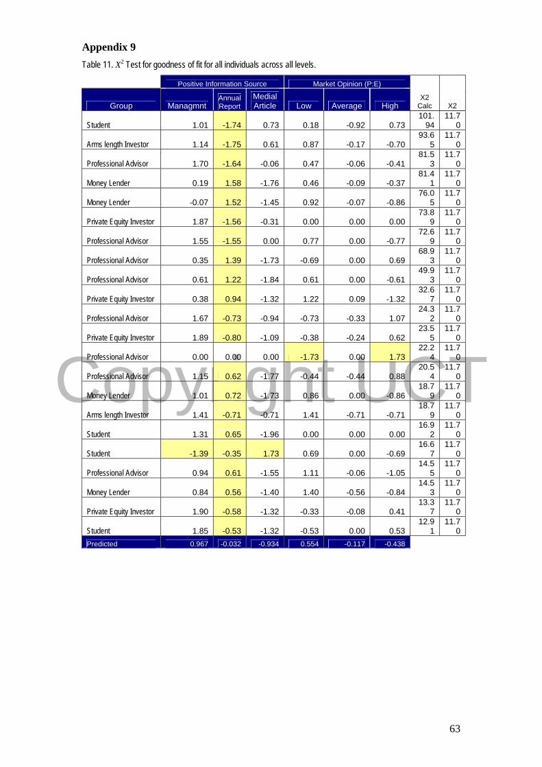
Copyright UCT

Appendix 9 Table 11. X2 Test for goodness of fit for all individuals across all levels.

Positive Information Source Market Opinion (P:E)

Group Managmnt Annual Report

Medial Article Low Average High

X2 Calc X2

Student 1.01 -1.74 0.73 0.18 -0.92 0.73 101.

94 11.7

0

Arms length Investor 1.14 -1.75 0.61 0.87 -0.17 -0.70 93.6

5 11.7

0

Professional Advisor 1.70 -1.64 -0.06 0.47 -0.06 -0.41 81.5

3 11.7

0

Money Lender 0.19 1.58 -1.76 0.46 -0.09 -0.37 81.4

1 11.7

0

Money Lender -0.07 1.52 -1.45 0.92 -0.07 -0.86 76.0

5 11.7

0

Private Equity Investor 1.87 -1.56 -0.31 0.00 0.00 0.00 73.8

9 11.7

0

Professional Advisor 1.55 -1.55 0.00 0.77 0.00 -0.77 72.6

9 11.7

0

Professional Advisor 0.35 1.39 -1.73 -0.69 0.00 0.69 68.9

3 11.7

0

Professional Advisor 0.61 1.22 -1.84 0.61 0.00 -0.61 49.9

3 11.7

0

Private Equity Investor 0.38 0.94 -1.32 1.22 0.09 -1.32 32.6

7 11.7

0

Professional Advisor 1.67 -0.73 -0.94 -0.73 -0.33 1.07 24.3

2 11.7

0

Private Equity Investor 1.89 -0.80 -1.09 -0.38 -0.24 0.62 23.5

5 11.7

0

Professional Advisor 0.00 0.00 0.00 -1.73 0.00 1.73 22.2

4 11.7

0

Professional Advisor 1.15 0.62 -1.77 -0.44 -0.44 0.88 20.5

4 11.7

0

Money Lender 1.01 0.72 -1.73 0.86 0.00 -0.86 18.7

9 11.7

0

Arms length Investor 1.41 -0.71 -0.71 1.41 -0.71 -0.71 18.7

9 11.7

0

Student 1.31 0.65 -1.96 0.00 0.00 0.00 16.9

2 11.7

0

Student -1.39 -0.35 1.73 0.69 0.00 -0.69 16.6

7 11.7

0

Professional Advisor 0.94 0.61 -1.55 1.11 -0.06 -1.05 14.5

5 11.7

0

Money Lender 0.84 0.56 -1.40 1.40 -0.56 -0.84 14.5

3 11.7

0

Private Equity Investor 1.90 -0.58 -1.32 -0.33 -0.08 0.41 13.3

7 11.7

0

Student 1.85 -0.53 -1.32 -0.53 0.00 0.53 12.9

1 11.7

0 Predicted 0.967 -0.032 -0.934 0.554 -0.117 -0.438

63

Copyright UCT

Appendix 10

Graphs and Statistics for Q. 2.4 Market Measures VS. Management Track Record.

Q2.4 Raw Data of Part-worths: Market Trend

-2.00-1.50-1.00-0.500.000.501.001.502.00

w w w w w w x x x x x y y y y y y y y z z z z z z z z z z z zz zz zz zz zz

Bull Market Bear Market

Q2.4 Raw Data of Part-worths: Beta

-1.00

-0.50

0.00

0.50

1.00

w w w w w w x x x x x y y y y y y y y z z z z z z z z z z z zz zz zz zz zz

High Beta Low Beta Q2.4 Raw Data of Part-worths: Management Track Record

-3.00

-2.00

-1.00

0.00

1.00

2.00

3.00

w w w w w w x x x x x y y y y y y y y z z z z z z z z z z z zz zz zz zz zz

Good Track Fair Track No Track Table 12. Level analysis for Market Measures vs. Management Track Record.

Market Trend Beta Management Track Record

Statistic Bull Bear High Low Good Fair None

χ2 test for normality p=0.246 p=0.246 p=0.056 p=0.056 p=0.000 p=0.411 p=0.000 Bartlett’s Test for Equal Variance p=1.000 p=1.000

Kruskal- Wallis p=0.000 Paired T-Test p=0.000 p=0.000

Table 13. Group analysis for Market Measures vs. Management Track Record.

Bull Market

Bear Market

High Beta

Low Beta

Good Track

Fair Track

No Track

Kruskal Wallis/ Anova 0.087 0.087 0.92 0.92 0.045 + 0.654 0.783

64

Copyright UCT

Appendix 11.

Table 14. X2 test for goodness of fit for al individuals across all levels.

Market Measures Management Track Record

Group Bull

Market Bear

Market High Beta

Low Beta

Good Track

Fair Track No Track

X2 Calc X2

Money Lenders 0.91 -0.91 0.91 -0.91 -1.36 0.00 1.36 13.59 12.59Money Lenders 0.27 -0.27 0.00 0.00 2.14 -1.07 -1.07 13.51 12.59Predicted 0.614 -0.614 0.311 -0.311 1.579 -0.080 -1.499

65

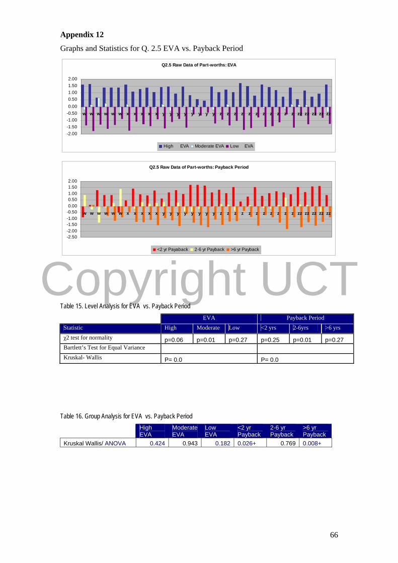
Copyright UCT

Appendix 12

Graphs and Statistics for Q. 2.5 EVA vs. Payback Period

Q2.5 Raw Data of Part-worths: EVA

-2.00-1.50-1.00-0.500.000.501.001.502.00

w w w w w w x x x x x y y y y y y y y z z z z z z z z z z z zz zz zz zz zz

High EVA Moderate EVA Low EVA

Q2.5 Raw Data of Part-worths: Payback Period

-2.50-2.00-1.50-1.00-0.500.000.501.001.502.00

w w w w w w x x x x x y y y y y y y y z z z z z z z z z z z zz zz zz zz zz

<2 yr Payaback 2-6 yr Payback >6 yr Payback

Table 15. Level Analysis for EVA vs. Payback Period

EVA Payback Period

Statistic High Moderate Low <2 yrs 2-6yrs >6 yrs

χ2 test for normality p=0.06 p=0.01 p=0.27 p=0.25 p=0.01 p=0.27 Bartlett’s Test for Equal Variance Kruskal- Wallis P= 0.0 P= 0.0

Table 16. Group Analysis for EVA vs. Payback Period

High EVA

Moderate EVA

Low EVA

<2 yr Payback

2-6 yr Payback

>6 yr Payback

Kruskal Wallis/ ANOVA 0.424 0.943 0.182 0.026+ 0.769 0.008+

66

Copyright UCT

Appendix 13 Table 17. Fisher’s LSD for level “< 2 yrs”

Students P. Equity Investors Prof Advisors Arms Length Investors Money Lendersmean 1.376 1.288 1.075 1.004 0.304

Fisher's L.S.D. <2 yr Payback

Coloured lines indicate treatments that are not statistically distinguishable Table 18. Fisher’s LSD for level “>6 yrs”

Money Lenders Prof AdvisorsArms Length Investors

Personal/ Private Equity Investors Students

mean -0.45282184 -1.12354172 -1.12946262 -1.23225562 -1.33804432

Coloured lines indicate treatments that are not statistically distinguishable

Fisher's L.S.D. >6 yr Payback

Table 19. X2 Test for goodness of fit for all individuals across all sectors

Economic Value Payback Period

Group High EVA

Moderate EVA

Low EVA

<2 yr Payback

2-6 yr Payback

>6 yr Payback

X2 Calc X2

Money Lenders 0.65 0.65 -1.31 1.31 -1.31 0.00 75.58 11.70 Money Lenders 1.40 -0.51 -0.89 -0.51 1.40 -0.89 63.65 11.70 Money Lenders 1.58 -0.23 -1.35 -0.90 0.90 0.00 26.05 11.70 Prof Advisor 0.71 -0.14 -0.57 1.13 0.71 -1.84 13.09 11.70 Predicted 1.185 -0.015 -1.169 1.024 0.040 -1.065

67

Copyright UCT

Appendix 14.

Graphs and Statistics for Q2.6 External Competition vs. Internal Risk

Q2.6 Raw Data of Part-worths: External Competition

-2.50-2.00-1.50-1.00-0.500.000.501.001.502.00

w w w w w w x x x x x y y y y y y y y z z z z z z z z z z z zz zz zz zz zz

Collabourate Cooperative Fierce comp

Q2.6 Raw Data of Part-worths: Internal Risk

-2.00-1.50-1.00-0.500.000.501.001.502.00

w w w w w w x x x x x y y y y y y y y z z z z z z z z z z z zz zz zz zz zz

Niche Franchise New Bus

Table 20. Level Analysis for External Competition vs. Internal Risk

External Competition Internal Risk

Statistic Collaborate Cooperative Fierce comp Niche Franchise New Bus χ2 test for normality p=0.01 p=0.08 p=0.61 p=0.48 p=0.21 p=0.02 Bartlett’s Test for Equal Variance Kruskal- Wallis P= 0.0 P= 0.0

Table 21. Group Analysis for External Competition vs. Internal Risk

Collaborate Cooperative Fierce comp Niche Franchise

New Bus

Kruskal Wallis/ ANOVA 0.1513 0.591 0.884 0.363 0.737 0.97 Table 22. X2 Test for goodness of fit across all levels

Competitive Risk Internal Risk

Group Collaborate Cooperative Fierce comp Niche Franchise New Bus

χ2 Calc χ2

Prof Advisor -1.28 1.66 -0.38 -0.38 -0.60 0.98 25.28 11.70 Prof Advisor 1.09 0.16 -1.24 0.31 1.09 -1.40 13.91 11.70 Predicted 1.034 0.257 -1.291 0.969 0.077 -1.046

68

Copyright UCT

References Bonner S. (1990) Experience effects in auditing: the role of task-specific knowledge. The Accounting Review, 65 pp 72–92. Brandenburger A. M. and Nalebuff B.J. (1995) The right Game: Use Game Theory to Shape Strategy. Harvard Business Review pp 57-70. Byrne D. (1971) in Franke N., Gruber M., Harhoff D., and Henkel J. (2006) What you are is what you like—similarity biases in venture capitalists’ evaluations of start-up teams. Journal of Business Venturing 21 p 803. Chemanura T. J. and Paeglis I. (2005) Management quality, certification, and initial public offering. Journal of financial Economics May2005, Vol. 76 Issue 2, p 331-368. Clark-Murphy M. and Soutar G. (2005) Individual Investor Preferences: A Segmentation Analysis The Journal of Behavioral Finance, Vol. 6, No. 1, pp 6–14. Correia C., Flynn D., Uliana E.and Wormald M. (2003) Financial Management fifth Edition Juta and Co Ltd. Damodaran A. (2002) Investment Valuation. Tools and techniques for determining the value of any asset. John Wiley and Sons Inc. N.Y. Davis J. T. (1996) Experience and auditors’ selection of relevant information for preliminary control risk assessments. Auditing: A Journal of Practice and Theory, 15, 16–37. De Clercq D., Fried V. H., Lehtonen O., and Sapienza H. J. (2006) An Entrepreneur’s Guide to the Venture Capital Galaxy Academy of Management Perspectives, August, pp 90-112 . De Long J. B., Shleifer A., Summers L.and Waldmann R. J. (1991) The survival of Noise Traders in financial Markets . Journal of Business, Jan91, Vol. 64 (1) pp 1-19. Kimmel A.J. (2004) Editorial comment Journal of Behavioural Finance Vol 5 (3) Ernst and Young (1999) Mergers and Acquisitions: Review of Merger and Acquisition Activity Ernst and Young, Johannesburg Franke N., Gruber M., Harhoff D., and Henkel J. (2006) What you are is what you like—similarity biases in venture capitalists’ evaluations of start-up teams. Journal of Business Venturing 21 pp 802– 826. Fried V.H. and Hirsch R.D. (1994) Toward a Model of Venture Capital Investment Decision Making Financial Management Vol 23, No 4. pp 28-37. Gilbert E. (2003) Do managers of South African manufacturing firms make optimal capital investment decisions? South African Journal of Business Management 34(2) pp 11-18

69

Copyright UCT

Gilbridge T.J. (2004) A Choice Model with Conjunctive, Disjunctive and Compensatory Screening Rules Marketing Science Vol. 23 No. 3 pp 391-406. Grable J. and Lyttleton R.H. (1999) Financial risk tolerance revisited: The Development of a Risk assessment Instrument financial Service Reviews Vol 8 No.3 pp161-83. Green P.E. and Srinivasan V. (1990) Conjoint Analysis in Marketing: New Developments With Implications for Research and Practice Journal of Marketing, Oct90, Vol. 54 Issue 4 pp 3- 17. Gregory A (2001) Strategic Valuation of Companies Pearson Education Limited. Grinyer J.R. and Green C.D. (2003) Managerial advantages of using Payback Period as a surrogate for NPV. The Engineering Economist, Vol 48 No. 2. pp 152-168. Hair. J.F., Anderson R.E., Tatham, R.L., and Black, W.C. (1998) Multivariate Data Analysis 5th Ed. Prenitence Hall pp 403-418. Huber J., Wittink D.R., Fielder J.A. and Miller R. (1993) The effectiveness of Alternative Preference Elicitation Procedures in Predicting Choice. Journal of Marketing Research Vol. XXX Feb pp105-111. Johnson R.M. (2002) Gibson Errs on Points of Fact Marketing Research Spring 2002 Vol. 14 Issue 1 pp 47-48. Kaplan R.S. and Atkinson A. A.(1998) Advanced Management Accounting Prentice Hall. Li-Ping Tang T., Shin-Hsiung Tang D. and Luna-Arocas R. (2005) Money profiles: the love of money, attitudes, and needs. Personnel Review Vol. 34 No. 5, pp 603-618. Lo W. and Lin K. (2005) A Review of the effects of Investor Sentiment on Financial Markets: Implications for Investors International Journal of Management Vol. 22, pp 708-715. Nagy R.A. and Obenberger R.W. (1994) Factors Influencing Individual Investor Behavior Financial Analyst’s Journal July/ August pp 63-68. Olu-Tima T.O. (2003) Acceptable Project Investment Criteria AACE International Transactions INT.06 Porter M. (1990) The competitive advantage of nations N.Y. Free Press pp. 603-618 Riquelme H. and Rickards T. (1992) Hybrid Conjoint Analysis: an estimation probe in new venture decisions Journal of Business Venturing, 7 pp 505-518 Sahlman W. (1990) The structure and governance of venture capital organizations Journal of Financial Economics 27, pp 473-521.

70

Copyright UCT

Sandberg W.R., Schweiger D.M., and Hofer C.W. (1988) The Use of Verbal Protocols in Determining Venture Capitalists Decision Processes. Entrepreneurship Theory and Practice, Winter, pp 8-20 Sansing R.C. (1992)Accounting and the Credibility of Management Forecasts Contemporary Accounting Research. Vol 9 No 1. pp 33-45 Shepherd D. A. and Zacharakis A. ( 1999) Conjoint Analysis: A new methodological approach for researching the decision policies of venture capitalists Venture Capital Vol 1, No 3 pp 197 -217. Shepherd D. A. and Zacharakis A. (2001) The venture capitalist–entrepreneur relationship: control, trust and confidence in co-operative behaviour Venture Capital Vol 3, No 2 pp129 -149 .

Stewart G.B. (1991) The Quest for Value Harper Business

Von Neumann J. and Morgenstern O.(1947) Theory of Games and Economic Behaviour in Nagy R.A. and Obenberger R.W. (1994) Factors Influencing Individual Investor Behaviour Financial Analyst’s Journal July/ August p 63 Weber C. E. (1995) Economic/ Industry/ Company Analysis: An Integrative Approach Financial Practice and Education Spring/ Summer 1995 pp 113-117.

71