A Congestion Management Approach Using …1 point estimate method ... reveals that the 2m+1 PEM provides the best performance among the Hong’s PEMs. So this paper uses the 2m+1 PEM

J Electr Eng Technol.2015; 10(?): 30-40 http://dx.doi.org/10.5370/JEET.2015.10.2.030

Copyright ⓒ The Korean Institute of Electrical Engineers

This is an Open-Access article distributed under the terms of the Creative Commons Attribution Non-Commercial License (http://creativecommons.org/ licenses/by-nc/3.0/)which permits unrestricted non-commercial use, distribution, and reproduction in any medium, provided the original work is properly cited.

30

A Congestion Management Approach Using Probabilistic Power Flow Considering Direct Electricity Purchase

Xu Wang* and Chuan-Wen Jiang†

Abstract – In a deregulated electricity market, congestion of the transmission lines is a major problem the independent system operator (ISO) would face. Rescheduling of generators is one of the most practiced techniques to alleviate the congestion. However, not all generators in the system operate deterministically and independently, especially wind power generators (WTGs). Therefore, a novel optimal rescheduling model for congestion management that accounts for the uncertain and correlated power sources and loads is proposed. A probabilistic power flow (PPF) model based on 2m+1 point estimate method (PEM) is used to simulate the performance of uncertain and correlated input random variables. In addition, the impact of direct electricity purchase contracts on the congestion management has also been studied. This paper uses artificial bee colony (ABC) algorithm to solve the complex optimization problem. The proposed algorithm is tested on modified IEEE 30-bus system and IEEE 57-bus system to demonstrate the impacts of the uncertainties and correlations of the input random variables and the direct electricity purchase contracts on the congestion management. Both pool and nodal pricing model are also discussed.

Keywords: PPF, Congestion Management, ABC, 2m+1 PEM, Direct electricity purchase

1. Introduction Congestion of transmission lines occurs when the

networks fail to accommodate all the desired transactions due to the system operating limits such as branch power flow limits, voltage limits, etc. Congestion in one or more transmission lines leads to higher risk of electricity con-sumption, even unexpected widespread power blackouts [1]. Various congestion management approaches suitable for traditional power systems without intermittent energy, have been reported in recent literatures. However, the global rapid growth of wind power capacity increases the uncertainties in congestion management. Therefore, it is necessary to propose an efficient and reliable method to process congestion problem with random variables.

Optimal rescheduling of generators is generally adopted to manage the congestion for its low-cost and simplicity. Ashwani Kumar proposed a zonal sensitivity-based optimum real and reactive power generation rescheduling method for congestion management [2]. Another technique for optimum selection of generators to be rescheduled is demonstrated in [3], which is based on generator sensitivities to the power flow on congested lines. Congestion management techniques in different deregulated electricity markets are estimated in [4]. Besides, congestion management scheme based on optimal power flow (OPF) is an excellent

alternative method in a power system with deterministic operational constraints.

An OPF-based congestion management approach proposed in [5] is based on the nodal pricing framework and the pool model. Another OPF-based scheme which aims to minimize both congestion and service costs is presented in [6]. Various kinds of traditional congestion management models are essentially the OPF problems associated with security constraints. As system with high level wind power integration has enhanced uncertainties, a noval probabilistic OPF-based congestion management approach is addressed in this paper.

Cumulants and Gram-Charlier expansion theory are combined to approximate the probabilistic distribution functions (PDFs) of transmission line flows in [7]. As the cumulant method can’t be used to process correlated input random variables, a two PEM [8] is applied. Literature [9] reveals that the 2m+1 PEM provides the best performance among the Hong’s PEMs. So this paper uses the 2m+1 PEM [9-10] to process the PPF in the congestion manage-ment. In recent years, compared with other heuristic mothods [11-14], ABC algorithm proposed by D. Karaboga [11] for fewer parameters, faster convergence and higher precision [12] has been widely used to solve complex nonlinear optimization problems, such as congestion management [13], OPF [14], etc.

Congestion management methods available in most literatures use simple power flow method without considering the uncertainties and correlations of the input variables. In this paper, the ABC algorithm combined with an extended 2m+1 PEM method is proposed to

† Corresponding Author: Dept. of Electrical Engineering, Shanghai Jiao Tong University, China. ([email protected])

* Dept. of Electrical Engineering, Shanghai Jiao Tong University, China. ([email protected])

Received: January 6, 2014; Accepted: December 10, 2014

ISSN(Print) 1975-0102ISSN(Online) 2093-7423

Xu Wang and Chuan-Wen Jiang

http://www.jeet.or.kr │ 3131 │ J Electr Eng Technol.2015;10(1): 31-55

process the complex congestion problem with correlated random injections. Moreover, the impact of direct electricity purchase on the results of congestion is discussed.

This paper is organized as follows. The mathematical formulation of the congestion management model is presented in Section 2. Section 3 gives the PPF model coupled with correlated variables in detail. In Section 4, the ABC algorithm coupling with the PPF model to solve the complex congestion problem is proposed. Section 5 gives several case studies. Finally, Section 6 provides the relevant conclusions.

2. Mathematical Formulation Congestion management is an optimization problem

aims to minimize the congestion cost while satisfying the system and unit constraints. This section gives the congestion management model based on both pool and nodal pricing model in detail.

2.1 Objective functions

2.1.1 Cost of rescheduling in the pool model [15-16]

In the pool model, the ISO determines the market-

clearing price Ci,M and the output PGi of generator i without considering system constraints aiming to minimize the cost of electricity purchase. The original total cost of electricity purchase can be calculated by:

,1

G

i

N

org G i Mi

C P C=

= ∑ (1)

where NG is the number of generators. When the congestion occurs, the cost of “constraint on” and “constraint off” generators are:

, ,

1 1

, , ,1 1

( ) ( )

( )( ( ))

on onG G

i i i i

off offG G

i i i i

N N

on G G i M G G i Mi i

N N

off G G i M i M G G i Mi i

C P P C P P C

C P P C C P P C

= =

= =

′ ′ ′= − +

′ ′ ′ ′= − − +

∑ ∑

∑ ∑ (2)

where on

GN and offGN are the number of “constraint on” and

“constraint off” generators, respectively; iGP′ is the output of generator i after rescheduling; ,i MC′ is the actual price bids submitted by generator i. Combining (1-2), the cost of rescheduling in the pool model is obtained: 1 on off orgC C C C= + − (3)

In the above formula, the superscript ‘ − ’ denotes the

expectation of the random variables.

2.1.2 Cost of breach of direct electricity purchase contract Actually, the direct electricity purchase contract is a kind

of bilateral transactions [16]. If there is no static and dynamic security violation, all the requested contracts or transactions should be satisfied. Otherwise, a breach of contract will occur. Mathematically, the breach cost of a direct electricity purchase contract at generator i can be calculated according to [16] as follows:

, , ,2

,

( ) ( ),

0,i dc i i M i i dc i

i dc i

P P k C P P PC

P P

⎧ ′ ′ ′′− ⋅ ⋅ >⎪= ⎨′≤⎪⎩

(4)

where Pi,dc is the trading power of the direct electricity purchase contract of generator i, P’

i is the actual active power of generation i, and k is a penalty coefficient of breach of contract.

2.1.3 Congestion cost in different modes

Combining (3-4), the objective function in the pool

mode is:

Minimize 1 1 2f C wC= + (5)

where w is a penalty coefficient trying to perform all the direct electricity purchase contracts.

Though the formula (4) is still applicable in the nodal pricing model [5], the objective function is modified to:

Minimize 2 2( , )

( )i j iji j S

f LMP LMP P wC∈

= − ⋅ +∑ (6)

where S is the set of the two endpoints of the branches; Pij is the active power flow from bus i to j; LMPi and LMPj is the nodal prices of bus i and j, which are two endpoints of a branch, respectively. All the nodal prices are calculated by minmizing the cost of generation.

2.2 Constrains and limits

2.2.1 Power flow equations

1

1

( cos sin )

( sin cos )

bus

bus

N

i i j ij ij ij ijj

N

i i j ij ij ij ijj

P V V G B

Q V V G B

=

=

⎧= +⎪

⎪⎨⎪ = −⎪⎩

∑

∑

θ θ

θ θ (7)

where Pi, Qi and Vi are the active power, reactive power and voltage amplitude of bus i, respectively; Gij and Bij are conductance and susceptance between bus i and j , respectively; Nbus is the number of buses; θij is the phase angle difference between bus i and j.


32 │ J Electr Eng Technol.2015;10(1): 30-40

2.2.2 Power constraints of generators

, 1, 2, ,i i i

i i i

min maxG G G

Gmin maxG G G

P P Pi N

Q Q Q

⎧ ≤ ≤⎪ =⎨≤ ≤⎪⎩

K (8)

where

i

minGP and

i

maxGP are the minimum and maximum active

power of generator i;i

minGQ and

i

maxGQ are the minimum and

maximum reactive power of generator i; PGi and QGi are the active and reactive power of generator i.

2.2.3 Bus voltage limits

( ) , 1, 2, ,min max

i i i i busPro V V V i N≤ ≤ ≥ = Kα (9)

where Pro(·) denotes the probability of the event (·); min

iV and maxiV are the lower and upper bound of voltage

amplitude of bus i; Vi is the voltage amplitude of bus i; αi is the confidence level of the bus i’s constraint.

2.2.4 Line power flow limits

( ) , 1,2, ,max

i i i branchPro PF PF i N≤ ≥ = Kβ (10)

where maxiPF are the upper limit of transmission power

flow of branch i; iPF is the power flow of branch i; βi is the confidence level of the branch i’s constraint; Nbranch is the number of the branches.

2.2.5 Direct electricity purchase contract

In a practical system, not all of the generators have

direct electricity purchase contract with loads and vice-versa. Mathematically, if a generator at bus i have this contract the active power inequality constraint of (8) is modified into:

,{ , }

i i i

min maxG i dc G Gmax P P P P≤ ≤ (11)

For the objective function has already considered the

penalty term of this constraint violation, only constraint (8) need to be taken into account.

3. PPF Model Managing To Process Correlations To perform the impact of the uncertainties of loads and

wind farms (WFs), probabilistic models are established. Since the correlations among loads and WFs do affect the power flows [17], a modified 2m+1 PEM [10] capable of processing the correlations is introduced.

3.1 Probabilistic load model

Generally, load demand is supposed to follow a normal

distribution [10, 17]. So the active and reactive power of

load bus L can be expressed by:

2

2

2

2

( )1( ) exp22

( )1( ) exp22

L

LL

L

LL

L PL

PP

L QL

QQ

Pf P

Qf Q

⎛ ⎞−= ⎜ ⎟⎜ ⎟

⎝ ⎠⎛ ⎞−

= ⎜ ⎟⎜ ⎟⎝ ⎠

μσπσ

μσπσ

(12)

where LPμ and LPσ are the mean and standard deviation of active load; LQμ and LQσ are the mean and standard deviation of reactive load; exp(·) represents the exponential function.

3.2 Probabilistic correlated WFs model

Different from the probabilistic load model, the output

of WFs depends on the wind speed which follows the Weibull distribution. Thus, the joint PDF of the correlated WFs’ output at bus t can be obtained through the correlated wind speed using Monte Carlo method.

The PDF and cumulative distribution function (CDF) of the wind speed vj of the j-th WF at bus t are as follows [10]:

1 ( / )

( / )

( ) ( ) 0

( ) 1 0

k jj j j

k jj j

k vj jj j j

j j

vj j j

k vf v e v

F v e v

− −

−

= ≥

= − ≥

λ

λ

λ λ (13)

where kj is the shape factor and λj is the scale factor of vj. Weibull distributed wind speed can be transformed into normally distributed variable through Nataf transformation.

The correlated wind speed sampling matrix ,s WFs tN NV × = ,1 2[ , , , ]

WFs tNv v vL (Ns represents the sampling times) of the NWFs,t WFs at bus t can be generated as follows:

1. Generate a matrix , ,1 2[ , , , ]s WFs t WF tN N NR r r r× = L by the

Matlab random number generator which represents NWFs,t independent standard normal distributed random variables.

2. For the given correlation coefficient matrix Cg of the wind speeds, the modified correlation coefficient matrix Cmd by the Nataf transformation [19] are obtained using [10, 20]:

mn mnG′ =ρ ρ (14)

2

2 2

1.063 0.004 0.2( ) 0.001

0.337( ) 0.007 ( ) 0.007mn m n mn

m n mn m n m n

G = − − + −

+ + + + −

ρ γ γ ρ

γ γ ρ γ γ γ γ (15)

Where and mn′ρ are the elements at m-th row, n-th column of Cg and Cmd, respectively; mγ and nγ are the coefficients of variation of vm and vn. Then decompose Cmd by the Cholesky decomposition method [10, 21] into Cm=LLT, where L is an inferior triangular matrix.



3. Using the transformation Y=LR and the inverse Nataf transformation vj=Fj

-1(Φ(Y)), we can obtain the matrix , ,1 2[ , , , ]

s WFs t WFs tN N NV v v v× = L with NWFs,t Weibull distributed variables with a correlation coefficient matrix Cd.

Next, the wind speed vector vj from the j-th column of V

is used to determine the output column vector PWF,j [Ns× 1] of WF j with nj WTGs at the bus t as follows:

,

0( ) ( )

( )

0

j in

in j rj r j in r inWF j j

r j outj r

j out

v vv v vn P v v v v

P vv v vn P

v v

<⎧⎪ ≤ ≤− −⎪= ⎨ < ≤⎪⎪ >⎩

(16)

where Pr is the rated power of a single WTG; vin, vr and vout are the cut-in, rated and cut-out wind speed, respectively; nj is the number of WTGs at the bus t.

Applying V and (16), the output sampling matrix PWFs [Ns× 1] of bus t with NWFs,t WFs is calculated by:

,

,1

WFs tN

WFs WF jj

P P=

= ∑ (17)

Using PWFs, the mean μWFs,t and standard deviation σWFs,t

of the WFs’ output at bus t can be obtained:

,

1

2

, ,1

1 ( )

1 ( )

s

s

N

WFs t WFsis

N

WFs t WFs WFs tis

P iN

P iN

=

=

⎧=⎪

⎪⎨⎪ ⎡ ⎤= −⎣ ⎦⎪⎩

∑

∑

μ

σ μ (18)

where PWFs(i) is the i-th element of PWFs. The z-th (z>2) order standardized central moments of the bus t with WFs can be calculated as:

, , ,1

1 ( )sN

z zz t WFs WFs t WFs t

is

M P iN =

⎛ ⎞⎡ ⎤= −⎜ ⎟⎣ ⎦

⎝ ⎠∑ μ σ (19)

So far, probabilistic models of loads and WFs have been

established. No matter the random injections are continuous or discrete, the traditional 2m+1 PEM can be just applied to uncorrelated ones. Thus, Part C introduces a modified 2m+1 PEM capable of dealing with correlated random injections at each bus.

3.3 2m+1 PEM for correlated random variables

As mentioned above, independent input random variables

are required in the 2m+1 PEM proposed in [9, 10]. For this purpose, the orthogonal transformation [10] based on Cholesky decomposition method [21] is used. A detailed

description of the orthogonal transformation is given in [10], which can convert a set of correlated input variables into an uncorrelated one. Based on the principle of the 2m+1 PEM [10], processing the correlations of the input random variables is to process the correlations of their standardized central moments. The 2m+1 PEM for correlated input random variable is as follows:

Step 1. According to the correlation coefficient matrix of the input random variables p=[p1, p2,…, pm]T, obtain the variance-covariance matrix Cp. Then get the matrix B by the Cholesky decomposition method using Cp=LLT and B=L-1.

Step 2. Transform the correlated input variables p into a new set of independent variables q=[q1, q2,…, qm]T whose first four central moments satisfy:

( ), ,1

;

;

, 1, 2, , ; 3,4.l l l

q p

q m

mj j

q j li p j pi

B

I

b l m j=

=

=

= = =∑ K

μ μ

σ

λ λ σ (20)

where pμ and qμ are the mean vectors of p and q; pσ and qσ are the standard deviation vectors of p and q; Im is the m-dimensional identity matrix; ,lq jλ (j=3,4) are the coefficients of skewness and kurtosis of ql; bli is the element at the l-th row, i-th column of B.

Step 3. Calculate the new transformed pairs (ql,k, ωl,k) of independent q defining the new 2m+1 PEM using follows:

, , , 1, 2,3

l ll k q l k qq k= + ⋅ =μ ξ σ (21)

3

,, ,1 ,2

,3 2,4 ,3

( 1) , 1, 2( )

1 1

k

l kl k l l

ll l

k

m

−⎧ −= =⎪ −⎪

⎨⎪ = −⎪ −⎩

ωξ ξ ξ

ωλ λ

(22)

where ,l kξ can be calculated by:

,3 3 2

, ,4 ,3

,3

3( 1) , 1, 22 4

0

l

l l

q kl k q q

l

k−= + − − =

=

λξ λ λ

ξ (23)

Step 4. Construct the new 2m+1 points in the form

1 ,( , , , , ), 1,2mq l k qq k =L Lμ μ and 1

( , , , , )l mq q qL Lμ μ μ . Let

q2m+1,k, k=1, 2, 3, be a m× m matrix each row of which is one point of the 2m+1 points with l from 1 to m. Then transform the 2m+1 points to the original space using p2m+1,k=B−1q2m+1,k.

Step 5. Calculate the deterministic power flow for each row of p2m+1,k for 2m+1 times using:

1 2 ,

1, 2,( , ) ( , , , , , ),

1, 2mi i p p l k p

l ms l k Z p

kμ μ μ

==

=L

L L (24)



The solution vectors si(l , k) is obtained. Step 6. Estimate the the j-th raw moment using:

( )

1 2

2

,1 1

,31

( ) ( , )

[ ( , , , )] , 1,2,m

mjj

i l k ik l

mj

i p p p ll

E s s l k

Z j

ω

μ μ μ ω

= =

=

⎡ ⎤⋅⎣ ⎦

+ ⋅ =

∑∑

∑L L

(25)

And the PDF and CDF of the output random variable si

can be calculated through Gram-Charlier expansion [7, 16]:

(6)61

(6)61

( ) ( ) ( ) ( )1! 6!

( ) ( ) ( ) ( )1! 6!

i

i

i i i i i

i i i i

i si

s

cch S S S S

ccH S S S S

sS

′= + + +

′= Φ + Φ + + Φ

−=

L

L

ϕ ϕ ϕ

μσ

(26)

where ( )⋅ϕ and ( )Φ ⋅ are the PDF and CDF of standard normal distribution, respectively; ci are constant coefficients of which detailed calculation can refer to [7, 16]; isμ and isσ are the mean and standard deviation of si.

4. Solution Method A PPF model capable of managing correlated random

injections has been described in the previous section to simulate the uncertainties and correlations in a congestion management problem. This section will give a detailed introduction of the ABC algorithm coupling with the PPF model to solve the complex congestion model.

4.1 Overview of the ABC algorithm

Initially, the ABC algorithm is proposed for optimizing

numerical unconstrained problems, which is a swarm-based meta-heuristic algorithm [22]. Then it is modified in [23] to handle constrained optimization problems.

In the ABC algorithm, every food source represents a possible solution of an optimization problem, and nectar amount of a food source represents the fitness of the corresponding food source. The process of artificial bees’ searching for the best food source is the optimization process. The colony of artificial bees includes three groups of bees: employed bees, onlookers and scout bees. The search of food source implemented by the artificial bees can be summarized as following:

1. Employed bees find the food source within the neighborhood of the previous food source in their memory and record the nectar amount of the new food source.

2. According to the information offered by the employed bees, onlookers judge the merits of the food source and

select a food source probabilistically. 3. Employed bee at abandoned inferior food source

becomes a scout bee and starts search a new food source randomly.

The main steps of the ABC algorithm are as follows: Step 1. Initialize the randomly distributed food-source

positions Xi=[xi,1, xi,2, …, xi,d] (solutions population) according to the upper and lower limits of the decision variables, where i=1,2,…,N (N represents the number of employed bees, onlooker bees and food sources), xi,j (j=1,2,…,d) represents the j-th decision variable of the solution Xi and d is the number of decision variables.

Step 2. Compute the nectar amount of the food source Xi using their fitness values:

100 , 0

1100 , 0

i

ffFitness

f f

⎧ ≥⎪ += ⎨⎪ + <⎩

(27)

where f is the objective function value at solution Xi.

Step 3. Determine neighborhood positions for the employed bees according to the exiting food-source positions using:

, , , ,( )new old old

i j i j i j k jx x U x x= + − (28)

where xi,j is the j-th parameter of solution Xi that was selected to be modified; U is a random number between [-1,1]; k i≠ and {1,2, , }k N∈ K ; {1, 2, , }i N∈ K ;

{1,2, , }j d∈ K . Then record the fitness values of the new neighborhood positions using (27).

Step 4. If the fitness value of a new neighborhood position is larger than the old one, replace the old one with the new one; otherwise, keep the old one.

Step 5. Calculate the selection probability Probi of the solution Xi for the outlook bees applying:

0.9 0.1, 1, 2, ,ii

max

FitnessProb i N

Fitness= × + = K (29)

Step 6. Select the onlooker bee depending on the

probability value. For the selected onlooker bee Xi, a new neighborhood position is created using (28); else go to Step 8. Then record the fitness values of the new neighborhood positions using (27).

Step 7. Follow the Step 4. Step 8. Find the abandoned food sources for scout bees.

If a food source is still not updated by a predetermined number of trials known as ‘limit’ value maxLim , then that food source is abandoned and the corresponding employed bee becomes a scout. Otherwise, no abandoned food sources exist and go to Step 10.

Step 9. For an abandoned food source Xi, update it with



a completely new food source Vi through:

, ( ), 1, 2, ,min max mini j i j i iv x u x x j d= + − = K (30)

where ui is a random number between [0,1]; max

ix and minix are the maximum and minimum parameter of Xi,

respectively. Step 10. Storage the global best solution obtained so far. Step 11. If the current iteration number (Iter) is larger

than the maximum iteration number of the search process (Itermax), stop and output the results. Otherwise, go back to Step 3.

There are three control parameters need to be set: 1) food-source size N, representing the number of employed bees or onlooker bees; 2) ‘limit’ value, which is the number of trials determining a food-source position abandoned or not (at least 0.5× N× d suggested in [11]); 3) Itermax, that is the maximum iteration number.

4.2 Congestion management strategy

After alleviating congestion in transmission grids, the

congestion may occur again due to the uncertainties and correlations of loads and wind power. Moreover, direct electricity purchase contracts affect the rescheduling of generators obviously. In case of congestion again, all the generators participating in congestion management must be rescheduling properly. This paper proposes a congestion management approach using PPF considering direct electricity purchase. If congestion cannot be removed just by rescheduling, a breach of contract is done between contracted parties based on its liquidated damage.

This paper uses the following methods to handle the constraints (7-10). Mathematically, equality constraint (7) is solved during the determined power flow calculation. Inequality constraint (8) can be handled as follows:

if

i i

minG GP P< ,

i i

minG GP P= ;

if i i

maxG GP P> ,

i i

maxG GP P= .

Reactive power constraints of generators are processed

by the similar method. Besides, if reactive power generation of any PV bus gets violated, the PV bus is treated as PQ bus.

The chance constraints (9) and (10) are handled as follows:

4.2.1 Calculate the penalty terms:

1

1

_

_

bus

line

Ni

max mini i i

Ni

maxi i

VPen V

V V

PPen P

P

=

=

Δ=

−

Δ=

∑

∑ (31)

where Pen_V and Pen_P are the penalty terms of bus voltage limits and line power flow limits; ΔVi and ΔPi are computed by:

{ }0, (9)

, ,i min down up maxi i i i

sV

max V V

atis

V V els

fied

e⎧⎪Δ = ⎨ − −⎪⎩

(32)

max

0, (10),i up

i i

atisfiedsP

P P else⎧

Δ = ⎨ −⎩ (33)

where Pro(Vi<Vi

down) = 1–αi, Pro(Vi>Viup) = 1–αi, and

Pro(|Pi|>Piup) = 1–βi.

4.2.2 Modify the original objective function f into:

_ _new V Pf f w Pen V w Pen P= + + (34)

where wV and wP are the penalty factors.

4.3 ABC algorithm coupling with PPF model

ABC algorithm coupling with PPF model is proposed

to solve the congestion management problem with correlated random injections. The flowchart of the proposed

iProb iX

iX

iProb

oldiFitness iX

_Pen Vnewf

_Pen P

newiX new old

i iFitness Fitness≥

newiFitness

1i iLim Lim= +

iX

0iLim = iX

i maxLim Lim≤

maxIter Iter<

0iLim =

1Iter Iter= +

Fig. 1. Flowchart for the ABC algorithm coupling with PPF



ABC algorithm is illustrated in Fig. 1. Further studies in [22-28] has proved that the ABC algorithm has a better performance in results and solutions compared with other popular population-based and heuristic optimization algorithms.

5. System Studies The proposed congestion management approach has

been illustrated on the modified IEEE 30-bus test system [29-30] and IEEE 57-bus test system [31] in the pool model in 5.1 and 5.2. The performance of the ABC algorithm is compared with that of evolutionary algorithm (EA) [32] and particle swarm optimization (PSO) [32] in 5.1. Similar study of IEEE 30-bus is conducted in nodal pricing model in 5.3. All the studies are implemented in MATLAB 2012a.

5.1 Modified IEEE 30-bus case study

The modified IEEE 30-bus test system consists of 6

generators (Table 1), 41 branches, 20 load buses whose data are from Table 2-3 of [30], and 2 WFs located at bus 28 as shown in Fig. 2. The active power consumption of each load is considered to be normally distributed with means equal to the values provided in Table 3 of [30] with the value at bus 5 zeroed out, and standard deviations of 10% with respect to such mean values. For simplicity, the power factor of each load is kept constant. Each WF

contains five 3MW WTGs and the wind speed is assumed to follow the Weibull distribution with scale and shape parameters 9, 2.205, respectively. Both WFs are correlated with a correlation coefficient 0.9 and a power factor 0.9 lag. Besides, the involved parameters are set as follows: wV=106, wP=106, Itermax=200 and Limmax=100.

Firstly, the original outputs of the generators are calculated by minimizing the electricity purchase cost without constraints (9)-(11). Here, the output of the WFs and the loads are assumed to be independent and the correlation coefficients among load buses are rL. Table 2 gives the details of the line congestion in condition of the original outputs with rL=0, 0.2, 0.4, 0.5, 0.6, 0.8, 0.9, respectively. From Table 2, with rL increased from 0 to 0.9, the standard deviation of the power flow through the congested line 6-8 grows from 3.7584MVA to 3.9340 MVA, which means a 4.67% increase, while the expected power flow has no significant increase. Also, if the confidence level of the chance constraints (9)-(10) is 0.95, branch 6-8 is the only congested line.

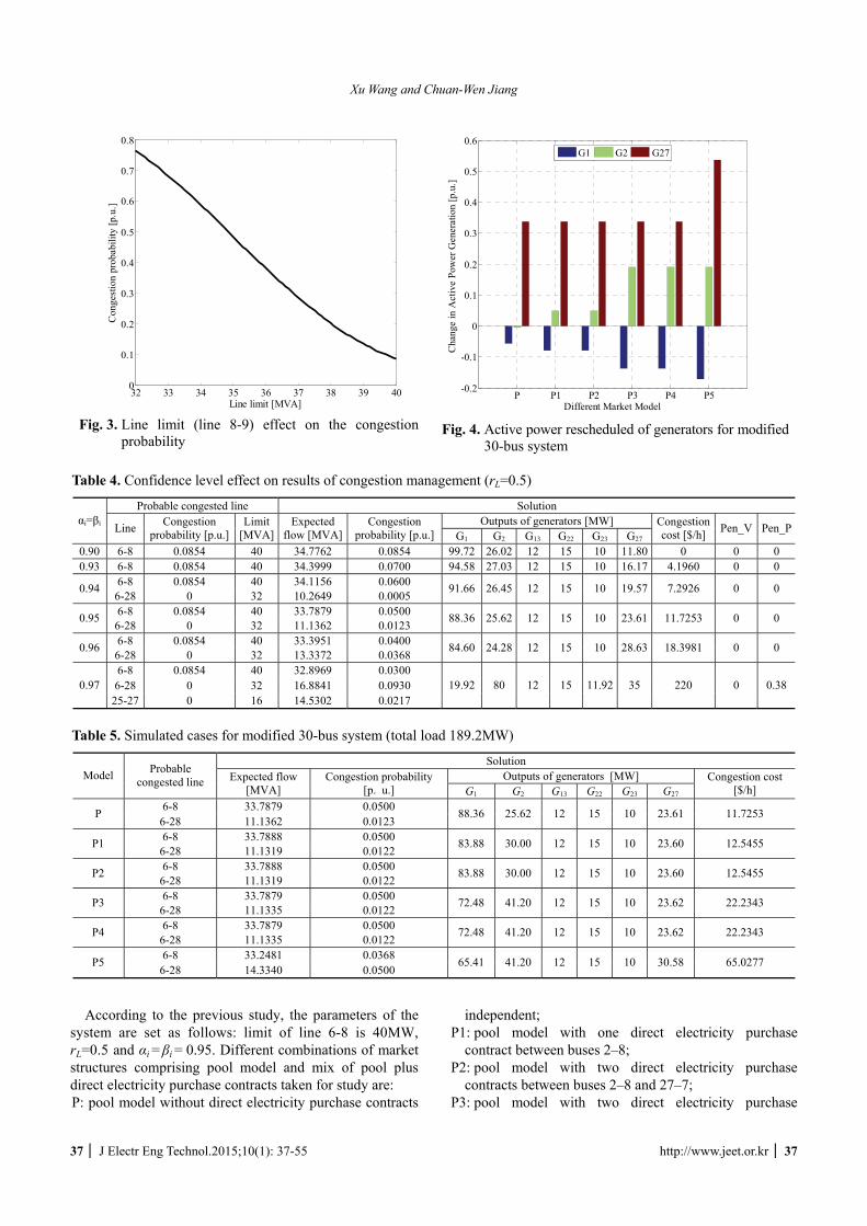
Fig. 3 illustrates the evolution of the congestion probability of branch 6-8 with rL=0.5. As the line limit increase from 32MW to 40MW, the congestion probability decrease from 0.7662 to 0.0854. In order to obtain a wide range of feasible region for congestion management, the line limit of branch 6-8 is raised to 40MW. Table 4 gives the simulated results of the congestion management with rL = 0.5 under different confidence levels. From the table, the cost of congestion management increases obviously with the confidence level raises, especially when αi = βi>0.95. What’s more, when αi = βi = 0.97, Pen_P>0 which means the line congestion can’t be eliminate just by reschedule the generators. To avoid the violations without load shedding, the line connected with or near the WFs must be expanded.

Table 2. Probable congested line details of 30-bus system with different rL (Line limit 32MVA)

rL

Probable Congested

Line

Expected Power Flow

[MVA]

Standard Deviation [MVA]

Congestion Probability

[p. u.] 0 6-8 34.7745 3.7584 0.7788

0.2 6-8 34.7752 3.7982 0.7724 0.4 6-8 34.7758 3.8376 0.7761 0.5 6-8 34.7762 3.8571 0.7662 0.6 6-8 34.7765 3.8766 0.7695

6-8 34.7772 3.9105 0.7771 0.8 21-22 26.8959 2.4617 0.0147 6-8 34.7775 3.9340 0.7337 0.9 21-22 26.9009 2.5558 0.0308

Table 3. Comparison results of different algorithms

Expected power flow [MVA] Method Congestion cost

[$/h] line 6-8 Line 6-28

ABC 11.7253 33.7879 11.1362 EA 12.6368 33.7889 11.5247 PSO 12.2429 33.7878 11.4813

Fig.2. Modified IEEE 30-bus test system

Table 1. Generator data for modified 30-bus system

Bidding coefficients Bus

No. Pmax

[MW] Pmin

[MW] Qmax

[MW] Qmin

[MW] a b

1 200 50 250 -20 0.0075 2.002 80 20 100 -20 0.035 1.753 40 12 60 -15 0.05 3.0022 50 15 80 -15 0.125 1.0023 30 10 50 -10 0.05 3.0027 35 10 80 -15 0.01668 3.25

Bidding function: fB(P)= a P + b $/MWh



According to the previous study, the parameters of the system are set as follows: limit of line 6-8 is 40MW, rL=0.5 and αi = βi = 0.95. Different combinations of market structures comprising pool model and mix of pool plus direct electricity purchase contracts taken for study are: P: pool model without direct electricity purchase contracts

independent; P1: pool model with one direct electricity purchase

contract between buses 2–8; P2: pool model with two direct electricity purchase

contracts between buses 2–8 and 27–7; P3: pool model with two direct electricity purchase

32 33 34 35 36 37 38 39 400

0.1

0.2

0.3

0.4

0.5

0.6

0.7

0.8

Line limit [MVA]

Con

gest

ion

prob

abili

ty [p

.u.]

Fig. 3. Line limit (line 8-9) effect on the congestion

probability

P P1 P2 P3 P4 P5-0.2

-0.1

0

0.1

0.2

0.3

0.4

0.5

0.6

Different Market Model

Cha

nge

in A

ctiv

e Po

wer

Gen

erat

ion

[p.u

.]

G1 G2 G27

Fig. 4. Active power rescheduled of generators for modified

30-bus system

Table 4. Confidence level effect on results of congestion management (rL=0.5)

Probable congested line Solution Outputs of generators [MW] αi=βi Line Congestion

probability [p.u.] Limit

[MVA] Expected

flow [MVA] Congestion

probability [p.u.] G1 G2 G13 G22 G23 G27 Congestion cost [$/h] Pen_V Pen_P

0.90 6-8 0.0854 40 34.7762 0.0854 99.72 26.02 12 15 10 11.80 0 0 0 0.93 6-8 0.0854 40 34.3999 0.0700 94.58 27.03 12 15 10 16.17 4.1960 0 0

6-8 0.0854 40 34.1156 0.0600 0.94 6-28 0 32 10.2649 0.0005

91.66 26.45 12 15 10 19.57 7.2926 0 0

6-8 0.0854 40 33.7879 0.0500 0.95 6-28 0 32 11.1362 0.0123 88.36 25.62 12 15 10 23.61 11.7253 0 0

6-8 0.0854 40 33.3951 0.0400 0.96 6-28 0 32 13.3372 0.0368 84.60 24.28 12 15 10 28.63 18.3981 0 0

6-8 0.0854 40 32.8969 0.0300 6-28 0 32 16.8841 0.0930 0.97

25-27 0 16 14.5302 0.0217 19.92 80 12 15 11.92 35 220 0 0.38

Table 5. Simulated cases for modified 30-bus system (total load 189.2MW)

Solution Outputs of generators [MW] Model Probable

congested line Expected flow [MVA]

Congestion probability [p. u.] G1 G2 G13 G22 G23 G27

Congestion cost [$/h]

6-8 33.7879 0.0500 P 6-28 11.1362 0.0123

88.36 25.62 12 15 10 23.61 11.7253

6-8 33.7888 0.0500 P1 6-28 11.1319 0.0122

83.88 30.00 12 15 10 23.60 12.5455

6-8 33.7888 0.0500 P2 6-28 11.1319 0.0122 83.88 30.00 12 15 10 23.60 12.5455

6-8 33.7879 0.0500 P3 6-28 11.1335 0.0122 72.48 41.20 12 15 10 23.62 22.2343

6-8 33.7879 0.0500 P4 6-28 11.1335 0.0122

72.48 41.20 12 15 10 23.62 22.2343

6-8 33.2481 0.0368 P5 6-28 14.3340 0.0500

65.41 41.20 12 15 10 30.58 65.0277



contracts between buses 2–8, 12; P4: pool model with three direct electricity purchase

contracts between buses 2–8, 12 and 27-7; P5: pool model with four direct electricity purchase

contract between buses 2–8, 12 and buses 27–7, 24. Here, we assume that each direct electricity purchase

contract is the total active load consumption of the load bus, k=8 and w=10.

Table 3 gives the comparison results of the performance of ABC algorithm, EA [32] and PSO [32] for market structure P using the same population and iteration. From the table, the ABC algorithm has a better performance in the optimization results and can be used to solve the congestion problem properly.

The detailed simulated results and rescheduling of generators are present in Table 5 and Fig. 4. The table and the figure demonstrate that direct electricity purchase contracts decrease the feasible region of generation rescheduling. Comparing P1-P2 and P3-P4, the added contract between buses 27-7 have no effect on the existing contracts. However, some added contract may affect the rescheduling results significantly based on the comparison of P-P1, P1-P3 and P4-P5. Especially, in model P5, G27 needs to cut the contract by 0.92MW to make the system relieve the probable congestions. This can guide the generators to sign rational direct electricity purchase contracts.

5.2 Modified IEEE 57-bus case study

The modified IEEE 57-bus test system [31] consists of 7

generators, 80 branches and 42 load buses. WFs are located at bus 7 and 46 and each of them has 2 WFs with a correlation coefficient 0.9 and a power factor 0.9 lag. The two WF buses are correlated with a correlation coefficient 0.8 but they are both independent with other load buses. The characteristics of loads are set as the 30-bus system. Besides, we set the limit of branch 8-9 215MVA, rL=0.5, αi=βi=0.95, wV=109, wP=109, Itermax=200, Limmax=100, k=8 and w=103. Table 6 gives the detailed data of generators for the modified 57-bus system.

Different combinations of market structures comprising pool model and mix of pool plus direct electricity purchase contracts are as follows: C: pool model without any direct electricity purchase

contracts. C1: pool model with a direct electricity purchase contract

between buses 6-8. C2: pool model with two direct electricity purchase

contracts between buses 6-8 and 8-12 (320MW). C3: pool model with two direct electricity purchase

contracts between buses 6-8, 13. C4: pool model with three direct electricity purchase

contracts between buses 6-8, 13 and 8-12 (320MW). C5: pool model with three direct electricity purchase

contracts between buses 6-8, 13 and 8-12 (350MW). Here, all direct electricity purchase contracts are the total

active load consumption of the load bus except those with a brackets mark.

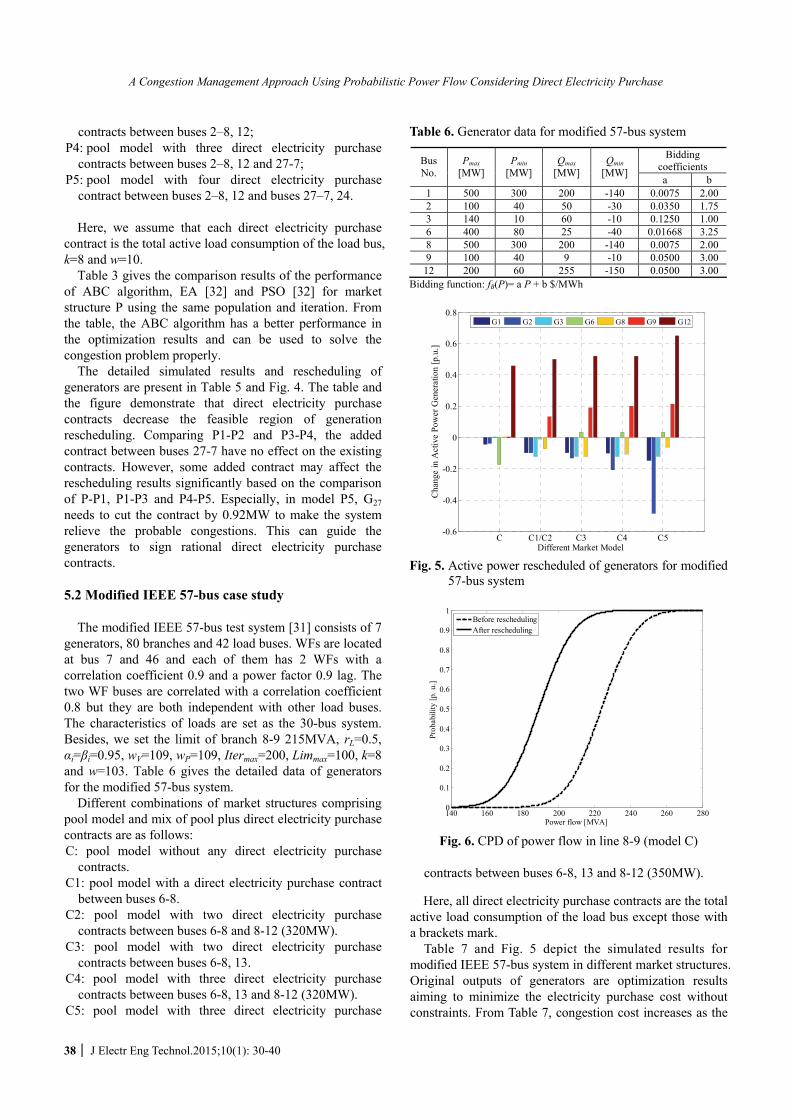
Table 7 and Fig. 5 depict the simulated results for modified IEEE 57-bus system in different market structures. Original outputs of generators are optimization results aiming to minimize the electricity purchase cost without constraints. From Table 7, congestion cost increases as the

Table 6. Generator data for modified 57-bus system

Bidding coefficients Bus

No.Pmax

[MW]Pmin

[MW]Qmax

[MW] Qmin

[MW] a b

1 500 300 200 -140 0.0075 2.002 100 40 50 -30 0.0350 1.753 140 10 60 -10 0.1250 1.006 400 80 25 -40 0.01668 3.258 500 300 200 -140 0.0075 2.009 100 40 9 -10 0.0500 3.0012 200 60 255 -150 0.0500 3.00

Bidding function: fB(P)= a P + b $/MWh

C C1/C2 C3 C4 C5-0.6

-0.4

-0.2

0

0.2

0.4

0.6

0.8

Different Market Model

Cha

nge

in A

ctiv

e Po

wer

Gen

erat

ion

[p.u

.]

G1 G2 G3 G6 G8 G9 G12

Fig. 5. Active power rescheduled of generators for modified

57-bus system

140 160 180 200 220 240 260 2800

0.1

0.2

0.3

0.4

0.5

0.6

0.7

0.8

0.9

1

Power flow [MVA]

Prob

abili

ty [p

. u.]

Before reschedulingAfter rescheduling

Fig. 6. CPD of power flow in line 8-9 (model C)



number of direct electricity purchase contracts grows overall. Some direct electricity purchase contracts added to the system have no effects on the original system (comparing C1-C2) but some may have (comparing C3-C4). In C5, in order to remove the congestion the contract between buses 8-12 is decreased by 8.35MW. As a result, signing direct electricity purchase contracts rationally can help relief congestion somehow. Cumulative probability distribution (CPD) of branch 8-9 before and after rescheduling for market structure C is presented in Fig. 6. The value of the power flow range decrease obviously through the rescheduling.

5.3 Nodal pricing model case study of IEEE 30-bus

All the relative parameters in this part are set as the same

as those in 5.1. Similar to the previous case studies, different combinations of market structures comprising nodal pricing model and mix of nodal pricing plus direct electricity purchase contracts are assumed, namely N, N1, N2, N3, N4, N5, respectively.

Table 8 shows the simulated optimization results for modified IEEE 30-bus system in nodal pricing model under different direct electricity purchase contracts. Based on the table, similar concolusions as those in 5.1 can be obtained. However, as the settlement of congestion cost in the nodal pricing model is quite different from that in the pool model, the results in Table 8 are quite different from those in Table 5. This indicates that suitable scheduling

approaches should be adopted in different market modes. Also, Table 8 demonstrates that the proposed congestion management model capable of processing uncertainties and correlations can be adoptd in the nodal pricing model.

6. Conclusion In this paper, a new congestion management approach

based on probabilistic power flow has been presented to process uncertainties and correlations in congestion problem. The probabilistic power flow model has been formed based on the combined method of 2m+1 PEM and Cholesky decomposition. An optimal probabilistic power flow model minimizing the congestion cost considering market structures with pool, nodal pricing and direct electricity purchase contracts has been studied. The simulated results on the modified IEEE 30-bus system and IEEE 57-bus system reveal the following conclusions.

1) The correlations between buses with WFs or loads have significant effect on the congestion probability but little effect on the expected power flow.

2) Higher confidence level leads to more congestion cost. Dispatchers can select appropriate confidence level according to the demand of system operation.

3) The congestion management approach based on probabilistic power flow provides a way to balance both congestion cost and congestion probability.

Table 7. Simulated cases for congested line 8-9 in modified 57-bus system (total load 1250.8MW)

Solution Outputs of generators [MW] Model Expected flow

[MVA] Congestion probability

[p. u.] G1 G2 G3 G6 G8 G9 G12 Congestion cost

[$/h] Original 223.7648 0.6121 409.19 88.79 27.09 154.75 373.24 63.43 66.92 0

C 188.9704 0.0408 386.77 84.94 27.15 85.41 373.55 63.50 158.70 1107.8421 C1 185.4570 0.0078 359.97 78.82 10 150.01 336.50 76.68 166.77 1311.3427 C2 185.4570 0.0078 359.97 78.82 10 150.01 336.50 76.68 166.77 1311.3427 C3 175.2216 0 359.83 75.50 10 168.06 311.83 82.34 170.76 1486.2954 C4 180.0232 0 357.96 67.89 10 168 320 83.56 170.76 1495.0329 C5 189.8497 0.0500 334.33 40 10 167.93 341.65 84.76 196.91 2759.9625

Table 8. Simulated cases in nodal pricing for modified IEEE 30-bus system (total load 189.2MW)

Solution Outputs of generators [MW] Model Probable

congested line Expected flow [MVA]

Congestion probability [p. u.] G1 G2 G13 G22 G23 G27

Congestion cost [$/h]

6-8 33.7876 0.0500 N 6-28 11.2037 0.0137

53.45 52.68 12.00 20.87 12.38 22.40 67.1183

6-8 33.7882 0.0500 N1 6-28 11.1835 0.0133

56.01 51.21 12.00 20.34 11.48 22.80 73.3141

6-8 33.7878 0.0500 N2 6-28 11.2841 0.0147 56.01 51.21 12.00 20.34 11.48 22.80 73.3141

6-8 33.7879 0.0500 N3 6-28 11.1806 0.0133 56.01 51.21 12.00 20.34 11.48 22.80 73.3141

6-8 33.7878 0.0500 N4 6-28 11.2443 0.0141

56.01 51.21 12.00 20.34 11.48 22.80 73.3141

6-8 33.2585 0.0370 N5 6-28 14.3340 0.0500

50.34 54.88 12.00 16.48 10.00 30.25 112.0610



4) Signing direct electricity purchase contracts rationally can help relief the congestion without burdening generation rescheduling.

5) The proposed congestion management model can be used in both pool and nodal pricing model.

Acknowledgements This work is supported by National High Technology

Research and Development Program 863 of China (2012 AA050204).

Reference

[1] Stoft S., “Power system economics: designing market for electricity”. IEEE Press & Wiley-Interscience, New York, USA, 2002.

[2] Ashwani Kumar, S. C. Srivastava and S. N. Singh, “A zonal congestion management approach using real and reactive power rescheduling,” IEEE Trans. Power Syst., vol. 19, no. 1, pp. 554-562, Feb. 2004.

[3] Sudipta Dutta and S. P. Singh, “Optimal rescheduling of generators for congestion management based on particle swarm optimization,” IEEE Trans. Power Syst., vol. 23, no. 4, pp. 1560-1569, Nov. 2008.

[4] K. L. Lo, Y. S. Yuen, and L. A. Snider, “Congestion management in deregulated electricity markets,” in Proc. Int. Conf. Electric Utility Deregulation and Re-structuring and Power Technologies, London, U.K., 2000, pp. 47-52.

[5] Singh H., Hao S. and Papalexoplulos A., “Transmis-sion congestion management in competitive electricity markets,” IEEE Trans. Power Syst., vol. 13, no. 2, pp. 672-680, May 1998.

[6] F. Jian and J. W. Lamont, “A combined framework for service identification and congestion manage-ment,” IEEE Trans. Power Syst., vol.16, no. 1, pp. 56-61, Feb. 2001.

[7] P. Zhang, S. T. Lee, “Probabilistic load flow com-putation using the method of combined cumulants and Gram-Charlier expansion,” IEEE Trans. Power Syst., vol. 19, no. 1, pp. 676-682, Feb. 2004.

[8] Gregor Verbiˇc and Claudio A. Cañizares, “Pro-babilistic optimal power flow in electricity markets based on a two-point estimate method,” IEEE Trans. Power Syst., vol. 21, no. 4, pp. 1883-1893, Nov. 2006.

[9] Juan. M. Morales and Juan. Pérez-Ruiz, “Point estimate schemes to solve the probabilistic power flow,” IEEE Trans. Power Syst., vol. 22, no. 4, pp. 1594-1601, Nov. 2007.

[10] J.M. Morales, L. Baringo, A.J. Conejo and R. Mı´nguez, “Probabilistic power flow with correlated wind sources,” IET Gener. Transm. Distrib., vol. 4, iss. 5, pp. 641-651, 2010.

[11] D. Karaboga, “An idea based on honey bee swarm for numerical optimization,” Technical Report-TR06, Erciyes University, Engineering Faculty, Computer Engineering Department, 2005.

[12] Karaboga D, and Basturk B, “On the performance of artificial bee colony (ABC) algorithm,” Applied Soft Computing, vol. 8, iss. 1, pp. 687-697, Jan. 2008.

[13] Deb, S., and Goswami, A.K, “Congestion manage-ment by generator rescheduling using artificial bee colony optimization technique,” 2012 Annual IEEE India Conference, INDICON 2012, pp. 909-914.

[14] Kiliç, U., and Ayan, K, “Optimizing power flow of AC-DC power systems using artificial bee colony algorithm,” International Journal of Electrical Power and Energy Systems, vol. 53, iss. 1, pp. 592-602, 2013.

[15] H. S. Jung, D. Hur, and J. K. Park, “Congestion cost allocation method in a pool model,” Generation, Transmission and Distribution, IEE Proceedings, vol. 150, pp. 604-610, 2003.

[16] M.S. Kumar and C.P. Gupta, “Congestion manage-ment in a pool model with bilateral contract by generation rescheduling based on PSO,” in Advances in Power Conversion and Energy Technologies (APCET), 2012 International Conference on, 2012, pp. 1-6.

[17] Kaigui Xie, Roy Billinton, “Considering wind speed correlation of WECS in reliability evaluation using the time-shifting technique,” Electr. Power Syst. Res., vol. 79, iss. 4, pp. 687-693, Apr. 2009.

[18] Y.Yuan, J. Zhou, P. Ju, J. Feuchtwang, “Probabilistic load flow computation of a power system containing wind farms using the method of combined cumulants and Gram-Charlier expansion,” IET Renewable Power Generation, vol. 5, iss. 6, pp. 448-454, Nov. 2011.

[19] Yan Chen, Jinyu Wen, Shijie Cheng, “Probabilistic load flow method based on Nataf transformation and Latin Hypercube Sampling,” IEEE Trans. Sustain-able Energy, vol. 4, no. 2, pp. 294-301, Apr. 2013.

[20] Peiling Liu and Armen Der Kiureghian, “Multivariate distribution models with prescribed marginal and covariances,” Probab. Eng. Mech., vol. 1, iss. 2, pp. 105-112, Jun. 1986.

[21] H. Yu, C.Y. Chung, K.P. Wong, H.W. Lee, and J.H. Zhang, “Probabilistic load flow evaluation with hybrid Latin hypercube sampling and Cholesky decomposition,” IEEE Trans. Power Syst. , vol. 24, no. 2, pp. 661-667, May 2009.

[22] K. Chandrasekaran and S.P. Simon, “Multi-objective unit commitment problem with reliability function using fuzzified binary real coded artificial bee colony algorithm,” IET Gener. Transm. Distrib., vol. 6, iss. 10, pp. 1060-1073, 2012.

[23] B. Basturk and D. Karaboga, “An artificial bee colony (ABC) algorithm for numeric function opti-



mization,” in Proc. IEEE Swarm Intell. Symp., Indianapolis, IN, May 12-14, 2006.

[24] D. Karaboga and B. Basturk, “A powerful and efficient algorithm for numerical function optimi-zation: Artificial bee colony (ABC) algorithm,” J. Global Optimiz., vol. 39, pp. 459-471, 2007.

[25] R.S. Rao, S.V.L. Narasimham, and M. Ramalingaraju, “Optimization of distribution network configuration for loss reduction using artificial bee colony algori-thm,” Int. J. Elect. Power Energy Syst. Eng., vol. 1, no. 2, pp. 116-122, 2008.

[26] D. Karaboga, B. B. Akay, and C. Ozturk, “Artificial bee colony (ABC) optimization algorithm for training feed-forward neural networks,” Lect. Notes Comput. Sci.: Modeling Decisions for Artif. Intell., vol. 4617, pp. 318-319, 2007.

[27] F.S. AbuMouti, M.E. ElHawary, “Optimal Distri-buted Generation Allocation and Sizing in Distribut-ion Systems via Artificial Bee Colony Algorithm,” IEEE Trans. Power Delivery, vol. 26, no. 4, pp. 2090-2101, Oct. 2011.

[28] Quanke Pan, Ling Wang and Kun Mao etc., “An Effective Artificial Bee Colony Algorithm for a Real-World Hybrid Flowshop Problem in Steelmaking Process, ” IEEE Trans . Automation Science and Engineering, vol. 10, no. 2, pp. 307-322, Apr. 2013.

[29] R. W. Ferrero, S. M. Shahidehpour and V. C. Ramesh, “Transaction analysis in deregulated power systems using game theory”, IEEE Trans. Power Syst. , vol. 12, no. 3, pp. 1340-1347, Aug. 1997.

[30] O. Alsac and B. Stott, “Optimal load flow with steady state security”, IEEE Trans. Power Syst. , vol. 93, no. 3, pp. 745-751, 1974.

[31] L. L. Freris and A. M. Sasson, “Investigation of the load flow problem,” Proc. Inst. Elect. Eng., vol. 115, no. 10, pp. 1459-1466, 1968.

[32] D.E. Goldberg, Genetic Algorithms in Search, Opti-mization and Machine Learning, Addison-Wesley Pub. Co., 1989.

Xu Wang He received the B.S. degree in electrical engineering from Southeast University, Nanjing, China, in 2010. Currently, he is pursuing the Ph.D. degree in the School of Electronic Information and Electrical Engineering, Shanghai Jiao Tong University, Shanghai, China. Chuan-Wen Jiang He received the M.S. and Ph.D. degrees from Huazhong University of Science and Technology, Wuhan, China, in 1996 and 2000, respectively, and completed his postdoctoral research in the School of Electronic Information and Electrical Engineering, Shanghai Jiao Tong University, Shanghai, China, in 2002. He is a Professor with the School of Electronic Information and Electrical Engineering, Shanghai Jiao Tong University. He is currently researching reservoir dispatch, load forecast in power systems, and the electrical power market.

Documents

A Congestion Management Approach Using …1 point estimate method ... reveals that the 2m+1 PEM provides the best performance among the Hong’s PEMs. So this paper uses the 2m+1 PEM