A Concise Lecture Note on Differential Equations

1 Introduction

Definition 1.1. A differential equation is a mathematical equation that relates some unknownfunction with its derivatives. A differential equation is called an ordinary differential equation (ODE)if it contains an unknown function of one independent variable and its derivatives. A differentialequation is called a partial differential equation (PDE) if it contains unknown multi-variable functionsand their partial derivatives.

Definition 1.2. A solution to a differential equation is a function that validates the differentialequations.

Example 1.3. The following three differential equations are identical (with different expression):

y1 + y = x+ 3 ,

dy

dx+ y = x+ 3 ,

f 1(x) + f(x) = x+ 3 .

The function y(x) = x+2 (or f(x) = x+2) and y(x) = x+2+ e´x (or f(x) = x+2+ e´x) are bothsolutions to the differential equation above.

Example 1.4. Let u :

"

R2 Ñ R(x, t) ÞÑ u(x, t)

be an unknown function. The differential equation

ut ´ ux = t ´ x

is a partial differential equation, and u(x, t) = x2 + xt+ t2 is a solution to the PDE above.

Definition 1.5. The order of a differential equation is the order of the highest derivative that appearsin the equation. A differential equation of order 1 is called first order, order 2 second order, etc.

Example 1.6. The differential equations in Example 1.3 and 1.4 are both first order differentialequations, while the equation y2 + xy13 = x7 and ut ´ uxx = x3 + t5 are second order equations.

Definition 1.7. The ordinary differential equation

F (t, y, y1, ¨ ¨ ¨ , y(n)) = 0

is said to be linear if F is linear (or more precise, affine) function of the variable y, y1, ¨ ¨ ¨ , y(n). Asimilar definition applied to partial differential equations.

1.1 Why do we need to study differential equations?

Example 1.8 (Spring with or without Friction).

mx = ´kx ´ rx .

Example 1.9 (Oscillating pendulum).

mLθ = ´mg sin θ

Example 1.10 (System of ODEs). Let p : [0,8) Ñ R+ denote the population of certain species. Ifthere are plenty of resource for the growth of the population, the growth rate (the rate of change ofthe population) is proportion to the population. In other words, there exists constant γ ą 0 suchthat

d

dtp(t) = γp(t) .

The LotkaVolterra equation or the predator-prey equation:

p1 = γp ´ αpq ,

q1 = βq + δpq .

Example 1.11. A brachistochrone curve, meaning "shortest time" or curve of fastest descent, is thecurve that would carry an idealized point-like body, starting at rest and moving along the curve,without friction, under constant gravity, to a given end point in the shortest time. For given twopoint (0, 0) and (a, b), where b ă 0, what is the brachistochrone curve connecting (0, 0) and (a, b)?

DefineX =

h : [0, b] Ñ Rˇ

ˇh(0) = 0, h(b) = a, h is differentiable on (0,b)(

andA =

φ : [0, b] Ñ Rˇ

ˇφ(0) = 0, φ(b) = 0, h is differentiable on (0,b)(

,

and suppose that the brachistochrone curve can be expressed as x = f(y) for some f P A. Then f

the minimizer of the functionalT (h) =

ż b

0

a

1 + h1(y)2?

´2gydy

or equivalently,

T (f) = minhPX

ż b

0

a

1 + h1(y)2?

´2gydy .

If φ : [0, b] Ñ R is differentiable such that φ(0) = φ(b) = 0. Then for t in a neighborhood of 0,f + tφ P X ; thus

F (t) ”

ż b

0

a

1 + (f + tφ)1(y)2?

´2gydy

attains its minimum at t = 0. Therefore,

F 1(0) =d

dt

ˇ

ˇ

ˇ

t=0

ż b

0

a

1 + (f + tφ)1(y)2?

´2gydy = 0 @φ P A .

By the chain rule,ż b

0

f 1(y)φ1(y)?

´2gya

1 + f 1(y)2dy = 0 @φ P A .

Suppose in addition that f is twice differentiable, then integration-by-parts implies that

´

ż b

0

[f 1(y)

?´2gy

a

1 + f 1(y)2

]1

φ(y) dy = 0 @φ P A

which further implies that [f 1(y)

?´2gy

a

1 + f 1(y)2

]1

= 0

since φ P A is chosen arbitrarily.Question: What if we assume that y = f(x) to start with? What equation must f satisfy?

Example 1.12 (Euler-Lagrange equation). In general, we often encounter problems of the type

minyPA

ż a

0

L(y, y1, t) dt , where A =

y : [0, a] Ñ Rˇ

ˇ y(0) = y(a) = 0(

.

Write L = L(p, q, t). Then the minimizer y P A satisfies

d

dtLq(y, y

1, t) = Lp(y, y1, t) .

The equation above is called the Euler-Lagrange equation.

Example 1.13 (Heat equations). Let u(x, t) defined on Ωˆ (0, T ] be the temperature of a materialbody at point x P Ω at time t P (0, T ], and c(x), ϱ(x), k(x) be the specific heat, density, and theinner thermal conductivity of the material body at x. Then by the conservation of heat, for anyopen set U Ď Ω,

d

dt

ż

Uc(x)ϱ(x)u(x, t) dx =

ż

BUk(x)∇u(x, t) ¨ N(x) dS , (1.1)

where N denotes the outward-pointing unit normal of U . Assume that u is smooth, and U is aLipschitz domain. By the divergence theorem, (1.1) implies

ż

Uc(x)ϱ(x)ut(x, t)dx =

ż

Udiv

(k(x)∇u(x, t)

)dx .

Since U is arbitrary, the equation above implies

c(x)ϱ(x)ut(x, t) ´ div(k(x)∇u(x, t)) = 0 @ x P Ω , t P (0, T ].

If k is constant, thencϱ

kut = ∆u ”

nÿ

i=1

B 2u

Bx2i.

If furthermore c and ϱ are constants, then after rescaling of time we have

ut = ∆u . (1.2)

This is the standard heat equation, the prototype equation of parabolic equations.

Example 1.14 (Minimal surfaces). Let Γ be a closed curve in R3. We would like to find a surfacewhich has minimal surface area while at the same time it has boundary Γ.

Suppose that Ω Ď R2 is a bounded set with boundary parametrized by (x(t), y(t)) for t P I, andΓ is a closed curve parametrized by (x(t), y(t), f(x(t), y(t))). We want to find a surface having C asits boundary with minimal surface area. Then the goal is to find a function u with the property thatu = f on BΩ that minimizes the functional

A (w) =

ż

Ω

a

1 + |∇w|2 dA .

Let φ P C 1(Ω), and define

δA(u;φ) = limtÑ0

A(u+ tφ) ´ A(u)

t=

ż

Ω

∇u ¨ ∇φa

1 + |∇u|2dx .

If u minimize A, then δA(u;φ) = 0 for all φ P C 1c (Ω). Assuming that u P C 2(Ω), we find that u

satisfiesdiv

( ∇ua

1 + |∇u|2

)= 0 ,

or expanding the bracket using the Leibnitz rule, we obtain the minimal surface equation

(1 + u2y)uxx ´ 2uxuyuxy + (1 + u2x)uyy = 0 @ (x, y) P Ω . (1.3)

Example 1.15 (System of PDEs - the Euler equations). Let Ω Ď R3 denote a fluid container, andϱ(x, t),u(x, t), p(x, t) denotes the fluid density, velocity and pressure at position x and time t. For agiven an open subset O Ď Ω with smooth boundary, the rate of change of the mass in O is the sameas the mass flux through the boundary; thus

d

dt

ż

Oϱ(x, t)dx = ´

ż

BO(ϱu)(x, t) ¨ N dS ,

where N is the outward-pointing unit normal of BO. The divergence theorem then implies that

d

dt

ż

Oϱ(x, t)dx = ´

ż

Odiv(ϱu)(x, t) dS .

If ϱ is a smooth function, then d

dt

ż

Oϱ(x, t)dx =

ż

Oϱt(x, t)dx; thus

ż

O

[ϱt + div(ϱu)

](x, t)dx = 0 .

Since O is chosen arbitrarily, we must have

ϱt + div(ϱu) = 0 in Ω . (1.4)

Equation (1.4) is called the equation of continuity.Now we consider that conservation of momentum. Let m = ϱu be the momentum. The conser-

vation of momentum states thatd

dt

ż

Om dx = ´

ż

BOm(u ¨ N) dS ´

ż

BOpN dS +

ż

Oϱf dx ,

here we use the fact that the rate of change of momentum of a body is equal to the resultant forceacting on the body, and with p denoting the pressure the buoyancy force is given by

ż

BOpN dS.

Here we assume that the fluid is invicid so that no friction force is presented in the fluid. Therefore,assuming the smoothness of the variables, the divergence theorem implies that

ż

O

[mt +

nÿ

j=1

B (muj)

Bxj+∇p ´ ϱf

]dx = 0 .

Since O is chosen arbitrarity, we obtain the momentum equation

(ϱu)t + div(ϱu b u) = ´∇p+ ϱf . (1.5)

Initial conditions: ϱ(x, 0) = ϱ0(x) and u(x, 0) = u0(x) for all x P Ω.Boundary condition: u ¨ N = 0 on BΩ.

1. If the density is constant (such as water), then (1.4) and (1.5) reduce to

ut + u ¨ ∇u = ´∇p+ f in Ω ˆ (0, T ) , (1.6a)

divu = 0 in Ω ˆ (0, T ) . (1.6b)

Equation (1.6) together with the initial and the boundary condition are called the incompress-ible Euler equations.

2. If the pressure p solely depends on the density; that is, p = p(ϱ) (the equation of state), then(1.4) and (1.5) together with are called the isentropic Euler equations.

1.2 Direction Fields

A direction field is in particular very useful in the study of first order differential equations of thetype:

dy

dt= f(t, y) ,

where f is a scalar function. A direction field is a vector-field on the (t, y)-plane on which a vector(1, f(t, y)) is associated with each point (t, y).

Example 1.16. Consider a falling object whose velocity satisfies the ODE

mdv

dt= mg ´ γv .

1.3 Initial and Boundary Conditions

Given y satisfies f(t, y, y1, ¨ ¨ ¨ , y(n)

)= 0, the initial condition for the ODE is of the form

y(a) = b1 , y1(a) = b2 , ¨ ¨ ¨ , y(n´1)(a) = bn

which specify the derivative of y at a up to (n ´ 1)-th derivative of y.If we are interested in an ODE of the form f

(x, y, y1, y2, ¨ ¨ ¨ , y(2n´1), y(2n)

)= 0 on a particular

interval [a, b], the boundary condition for an ODE of this type is of the form

y(a) = c1, y(b) = d1, y1(a) = c2, y

1(b) = d2, ¨ ¨ ¨ , y(n)(a) = cn+1, y(n)(b) = dn+1 .

2 First Order Differential Equations

In general, a first order ODE can be written as

dy

dt= f(t, y)

for some function f . In this chapter, we are going to solve the linear equation above explicitly with

1. f(t, y) = p(t)y + q(t);

2. f(t, y) = g(y)h(t),

and also provide some insight of nonlinear equations.

2.1 Linear Equations; Method of Integrating Factors

Suppose that we are given a first order linear equation

dy

dt+ p(t)y = q(t) with initial condition y(a) = b .

Let P (t) be an anti-derivative of p(t); that is, P 1(t) = p(t). Then

eP (t)(dydt

+ P 1(t)y)= eP (t)q(t) ñ

d

dt

(eP (t)y(t)

)= eP (t)q(t)

ñ

ż t

a

d

ds

(eP (s)y(s)

)ds =

ż t

a

eP (s)Q(s)ds ñ eP (t)y(t) ´ eP (a)y(a) =

ż t

a

eP (s)Q(s)ds

ñ y(t) = eP (a)´P (t)b+

ż t

a

eP (s)´P (t)Q(s)ds .

How about if we do not know what the initial data is? Then

eP (t)(dydt

+ P 1(t)y)= eP (t)q(t) ñ

d

dt

(eP (t)y(t)

)= eP (t)q(t) ñ eP (t)y(t) = C +

ż

eP (t)q(t)dt ,

whereż

eP (t)q(t)dt denotes an anti-derivative of ePQ. Therefore,

y(t) = Ce´P (t) + e´P (t)

ż

eP (t)q(t)dt

Example 2.1. Solve dy

dt+

1

2y =

1

2et/3. Answer: y(t) = 3

5et/3 + Ce´t/2.

Example 2.2. Solve dy

dt´ 2y = 4 ´ t. Answer: y(t) = ´

7

4+

1

2t+ Ce2t.

Example 2.3. Solve ty 1 + 2y = 4t2 with y(1) = 2. Answer: y(t) = t2 +1

t2.

2.2 Separable Equations

Suppose that we are given a first order linear equation

dy

dt= g(y)h(t) with initial condition y(a) = b ,

where 1/g is assume to be integrable. Let G be an anti-derivative of 1/g. Then

dy

dt= g(y)h(t) ñ

1

g(y)

dy

dt= h(t) ñ G1(y)

dy

dt= h(t)

ñd

dtG(y(t)) = h(t) ñ

ż t

a

d

dsG(y(s))ds = h(t) ñ G(y(t)) ´ G(y(a)) =

ż t

a

h(s)ds

ñG(y(t)) = G(b) +

ż t

a

h(s)ds ,

and y can be solved if the inverse function of G is known.

Example 2.4. Let y be a solution to the ODE dy

dx=

x2

1 ´ y2. Then x, y satisfies x3 + y3 ´ 3y = C

for some constant C.

Example 2.5. Let y be a solution to the ODE dy

dx=

3x2 + 4x+ 2

2(y ´ 1)with initial data y(0) = ´1. Then

y = 1 ´?x3 + 2x2 + 2x+ 4.

Definition 2.6 (Integral Curves). Let F = (F1, ¨ ¨ ¨ , Fn) be a vector field. A parametric curvex(t) =

(x1(t), ¨ ¨ ¨ , xn(t)

)is said to be an integral curve of F if it is a solution of the following

autonomous system of ODEs:

dx1dt

= F1(x1, ¨ ¨ ¨ , xn) ,

...dxndt

= Fn(x1, ¨ ¨ ¨ , xn) .

In particular, when n = 2, the autonomous system above is reduced to

dx

dt= F (x, y) ,

dy

dt= G(x, y) (2.1)

for some function F,G. Since at each point (x0, y0) =(x(t0), y(t0)

)on the integral curve,

dy

dx

ˇ

ˇ

ˇ

(x,y)=(x0,y0)=dy/dt

dx/dt

ˇ

ˇ

ˇ

t=t0

if dx

dt

ˇ

ˇ

ˇ

t=t0‰ 0, instead of finding solutions to (2.1) we often solve

dy

dx=G(x, y)

F (x, y).

Example 2.7. Find the integral curve of the vector field F(x, y) = (4+ y3, 4x´x3) passing through(0, 1). Answer: y4 + 16y + x4 ´ 8x2 = 17.

2.3 Modelling with First Order Equations

Example 2.8 (Mixing). At the very beginning, Q0 Kgs salt were dissolved in 100 liters of water.Afterward, salty water containing 1/4 Kg salt per liter enter the container at the speed r liters perminute, while at the same time r liters of the well-mixed solution leaves the tank every minute. IfQ(t) is the quantity (in Kgs) of salt in the container at time t, then

dQ

dt=r

4´rQ

100, Q(0) = Q0 .

To solve this ODE, we use the integrating factor and obtain that

dQ

dt+rQ

100=r

4ñ

d

dt

(ert/100Q(t)

)=r

4ert/100 ñ ert/100Q(t) = 25ert/100 + C

ñ Q(t) = 25 + Ce´rt/100

and the initial data implies that C = Q0 ´ 25. Therefore,

Q(t) = 25 + (Q0 ´ 25)e´rt/100 .

Using the separation of variables,

dQ

dt=

r

100(25 ´ Q) ñ

dQ

25 ´Q=

r

100dt ñ ´ log |25 ´ Q(t)| =

rt

100+ C

and the initial data implies that C = ´ log |25 ´ Q0|. Therefore,

|25 ´Q0|

|25 ´Q(t)|= ert/100 or Q(t) = 25 + (Q0 ´ 25)e´rt/100 .

Example 2.9 (Escape Velocity). By Newton’s second law of motion F = ma, we consider the

equation mdv

dt= ´

GMm

(R+ x)2. Note that on the surface x = 0, the forcing equals ´mg; thus GM

R2= g.

In other words, the equation becomes mdv

dt= ´

mgR2

(R+ x)2.

Suppose that v can be written as a function of the position x, then

mdv

dt= ´

mgR2

(R + x)2ñ

dv

dx

dx

dt= ´

gR2

(R + x)2ñ v

dv

dx= ´

gR2

(R + x)2ñ vdv = ´

gR2

(R + x)2dx

ñ1

2v2 =

gR2

R + x+ C ñ v(x) = ˘

c

v20 ´ 2gR +2gR2

R + x,

where v0 = v(0) is the initial data. For a given v0, the maximum attitude ξ that the body reaches is

given by ξ =v20R

2gR ´ v20, and to escape the gravity of the earth, the initial velocity v0 should be not

less than?2gR.

2.4 Differences b/w Linear and Nonlinear Equations

Concerns in differential equations: existence and uniqueness of solutions to differential equations.

Theorem 2.10. Let the function f be functions of t and y such that f and its partial derivative Bf

By

is continuous in some rectangular domain (t, y) P R ” (α, β)ˆ(γ, δ). Suppose that (t0, y0) P R. Thenin some interval t P (t0 ´ h, t0 + h) Ď (α, β), there exists a unique solution y = φ(t) to the initialvalue problem

y 1 = f(t, y) y(t0) = y0 .

Example 2.11. Consider dy

dt= y1/3 with initial data y(0) = 0. There are infinitely many solutions

y(t) =

#

0 if 0 ď t ă t0 ,

˘[23(t ´ t0)

] 32 if t ě t0 .

The reason for non-uniqueness of the solutions is that Bf

Byis not continuous near (0, 0).

Let us look at what separation of variables implies. Using the separation of variables, withG(y) =

3

2y3/2 we have

dy

dt= y1/3 ñ y´1/3dy

dt= 1 ñ G 1(y)

dy

dt= 1 ñ

dG

dt= 1 .

We cannot apply the fundamental theorem to conclude that G(t) = t + C here since dG

dtis not

continuous in the time interval containing t = 0 (in fact,ż

dG

dtdt is an improper integral). However,

if we apply the fundamental theorem of calculus, we obtain that

G(y(t)) = t+ C ñ y(t) =[23t] 3

2

which is one of the solutions.

2.5 Autonomous Equations and Population Dynamics

Definition 2.12. A first order ODE f(t, y, y1) = 0 is called autonomous if it can be rewritten as

dy

dt= f(y) .

Example 2.13 (Exponential Growth). In Chapter 1 we have discussed the equation

dp

dt= γp ,

where p is the population of certain species and γ is the rate of growth (or decline). Solving theODE with the initial data p(0) = p0, we obtain that

p(t) = p0eγt .

Example 2.14 (Logistic Growth). Instead of the purely theoretical model in Example 2.13, weconsider the equation

dp

dt= h(p)p ,

where the growth rate depends on the population. The simplest function for h is h(p) = γ ´ αp forsome positive constant α. Then

dp

dt= (γ ´ αp)p or equivalently dp

dt= γ

(1 ´

p

K

)p (2.2)

in which K =γ

α. Equation (2.2) is called the logistic equation.

Equilibrium solution: An equilibrium solution to a differential equation is a solution which doesnot vary with its independent variable (usually time). Therefore, there are two equilibrium solutionsto (2.2): p = φ1(t) = 0 and p = φ2(t) = K.General solution: Let p0 = p(0) ą 0 be the initial data. If p0 ‰ 0 or K, using separation ofvariables:

Kdp

(K ´ p)p= γdt ñ

( 1

K ´ p+

1

p

)dp = γdt ñ ´ log |K ´ p| + log |p| = γt+ C

ñp

|K ´ p|=

p0|K ´ p0|

eγt .

Therefore, p(t) =Kp0

p0 + (K ´ p0)e´γtwhich implies that p Ñ K as t Ñ 8, no matter p0 ą K or

0 ă p0 ă K. The solution p = φ2(t) = K is then called an asymptotically stable solution, whilep = φ1(t) = 0 is an unstable equilibrium solution. The number K is called the saturationlevel or the environmental carrying capacity.

Note that sinced2p

dt2=

d

dt

dp

dt=

d

dtf(p) = f 1(p)

dp

dt= f 1(p)f(p) ,

the graph of p versus t is concave up when f and f 1 have the same sign, while the graph is concavedown when f and f 1 have opposite signs. Therefore, solutions are concave up for 0 ă y ă

K

2

andy ą K, while the solutions are concave down for K

2ă y ă K.

Example 2.15 (A Critical Threshold). In Example 2.14, what happened if γ ă 0? In this case, weinstead consider

dp

dt= ´γ

(1 ´

p

T

)p , (2.3)

where γ ą 0 and T ą 0. This time the solution is

p(t) =Tp0

p0 + (T ´ p0)eγt

Unless p0 ě T , the population decays to zero; thus T is called the threshold level which means

below this level the growth of population does not occur. When p0 ą T , the time T ˚ =1

rlog p0

p0 ´ Tto which the population tends to infinite; thus the population becomes unbounded in a finite time.

The equilibrium solution p(t) = 0 is an asymptotically stable solution, while the equilibriumsolution p(t) = T is an asymptotically unstable solution.

Example 2.16 (Logistic Growth with a Threshold). Combining the experiences from the previoustwo examples, we design an model which cooperates the two phenomena:

1. the population will not grow if the initial population is below certain threshold;

2. the population will not blow up in a finite time if the population will grow.

Instead of letting h(p) = γ ´ αp, we consider the following more complicated situation: h(p) =

´γ(1 ´

p

T

)(1 ´

p

K

)for some γ ą 0 and 0 ă T ă K.

Equilibrium solution: φ1(t) = 0, φ2(t) = T , φ3(t) = K. φ1 and φ3 are asymptotically stable,while φ2 is asymptotically unstable.General solution: (Important or not?)

2.6 Exact Equations and Integrating Factors

Recall vector calculus:

Definition 2.17 (Vector fields). A vector field is a vector-valued function whose domain and rangeare subsets of Euclidean space Rn.

Definition 2.18 (Conservative vector fields). A vector field F : D Ď Rn Ñ Rn is said to beconservative if F = ∇φ for some scalar function φ. Such a φ is called a (scalar) potential for F onD.

Theorem 2.19. If F = (M,N) is a conservative vector field in a domain D, then Nx =My in D.

Theorem 2.20. Let D be an open, connected domain, and let F be a smooth vector field defined onD. Then the following three statements are equivalent:

1. F is conservative in D.

2.¿

CF ¨ dr = 0 for every piecewise smooth, closed curve C in D.

3. Given and two point P0, P1 P D,ż

CF ¨ dr has the same value for all piecewise smooth curves

in D starting at P0 and ending at P1.

Definition 2.21. A connected domain D is said to be simply connected if every simple closedcurve can be continuously shrunk to a point in D without any part ever passing out of D.

Theorem 2.22. Let D be a simply connected domain, and M,N,My, Nx be continuous in D. IfMy = Nx, then F = (M,N) is conservative.

Sketch of the proof. Since Nx =My,

N(x, y) = N(x0, y) +

ż x

x0

My(z, y) dz = N(x0, y) +B

By

ż x

x0

M(z, y) dz

=B

By

[Ψ(y) +

ż x

x0

M(z, y) dz],

where Ψ(y) is an anti-derivative of N(x0, y). Let φ(x, y) = Ψ(y) +ż x

x0

M(z, y) dz. Then clearly

(M,N) = ∇φ which implies that F = (M,N) is conservative. ˝

Combining Theorem 2.19 and 2.22, in a simply connected domain a vector field F = (M,M) isconservative if and only if My = Nx.

Example 2.23. Let D = R2zt(0, 0)u, and M(x, y) =´y

x2 + y2, N(x, y) =

x

x2 + y2. Then My = Nx =

y2 ´ x2

(x2 + y2)2in D; however, F ‰ ∇φ for some scalar function φ for it there exists such a φ, φ, up to

adding a constant, must be identical to the polar angle θ(x, y) P [0, 2π).

Now suppose that we are given a differential equation of the form

dy

dx= ´

M(x, y)

N(x, y),

in which separation of variables is not possible. We would like to find integral curves of the vectorfield F = (´N,M). Note that the ODE above is equivalent to that

M(x, y) +N(x, y)dy

dx= 0 .

Definition 2.24. An ODE of the form M(x, y) + N(x, y)dy

dx= 0 is called exact if there exists a

continuously differentiable function φ, called the potential function, such that φx =M and φy = N .

To solve the ODEM(x, y) +N(x, y)

dy

dx= 0 , (2.4)

the following two possibilities are most possible situations:

1. If My = Nx in a simply connected domain D, then Theorem 2.22 implies that the ODE (2.4)is exact in a simply connected domain D Ď R2; that is, there exists a potential function φ suchthat ∇φ = (M,N). Then (2.4) can be rewritten as

φx(x, y) + φy(x, y)dy

dx= 0 ;

and if (x(t), y(t)) is an integral curve, we must have

φx(x(t), y(t))dx

dt+ φy(x(t), y(t))

dy

dt= 0 or equivalently, d

dtφ(x(t), y(t)) = 0 .

Therefore, integral curve satisfies φ(x, y) = C.

2. If My ‰ Nx, we look for a function µ such that (µM)y = (µN)x in a simply connected domainD Ď R2. Such a µ always exists (in theory, but may be hard to find the explicit expression),and such a µ is called an integrating factor .

If such a µ exists, then µ satisfies

Mµy ´ Nµx + (My ´ Nx)µ = 0 .

Usually solving a PDE as above is as difficult as solving the original ODE.

Example 2.25. Solve (y cosx+ 2xey) + (sin x+ x2ey ´ 1)dy

dx= 0.

Let M(x, y) = y cosx + 2xey and N(x, y) = sinx + x2ey ´ 1. Then My(x, y) = cos x + 2xey =

Nx(x, y); thus the ODE above is exact. To find the potential function φ, due to the fact that φx =M

we find thatφ(x, y) = Ψ(y) +

ż

M(x, y)dx = Ψ(y) + y sinx+ x2ey

for some function Ψ. By φy = N , we must have Ψ 1(y) = ´1. Therefore, Ψ(y) = ´y + C; thus thepotential function φ is

φ(x, y) = y sinx+ x2ey ´ y + C .

Example 2.26. Solve (3xy + y2) + (x2 + xy)dy

dx= 0.

Let M(x, y) = 3xy + y2 and N(x, y) = x2 + xy. Then My ´ Nx = x + y. Assuming that theintegrating factor µ is only a function of x, then µ satisfies

dµ

dx=My ´ Nx

Nµ =

1

xµ ;

thus µ(x) = x.Multiplying both side of the ODE by µ, we then obtain

(3x2y + xy2) + (x3 + x2y)dy

dx= 0

which is exact, and the integral curves of the ODE above, by finding the potential, satisfies

x3y +x2y2

2= C .

One can also verify that the function µ(x, y) =1

xy(2x+ y)is also a valid integrating factor.

2.7 Numerical Approximations: Euler’s Method

The goal in this section is to solve the ODE

dy

dt= f(t, y) y(t0) = y0 (2.5)

numerically (meaning, programming in computer to produce an approximation of the solution) inthe time interval [t0, t0 + T ].

Let ∆t denote the time step (which mean we only care what the approximated solution is at timetk = t0 + k∆t for all k P N), and yk = y(t0 + k∆t). Since dy

dt(tk) «

yk+1 ´ yk∆t

when ∆t « 0, we

substitute yk+1 ´ yk∆t

for dy

dt(tk) and obtain

yk+1 « yk + f(tk, yk)∆t @ k P N .

The forward/explicit Euler method is the iterative scheme

uk+1 = uk + f(tk, uk)∆t @ k P

1, 2, ¨ ¨ ¨ ,[ T

∆t

]´ 1

(

, u0 = y0 (in theory) . (2.6)

Assume that f is bounded and has bounded continuous partial derivatives ft and fy; that is, ftand fy are continuous and for some constant M ą 0 |f(t, y)| + |ft(t, y)| + |fy(t, y)| ď M for all t, y.Then the mean value theorem implies that the fundamental theorem of ODE (which will be providedin the next section) provides a unique continuously differentiable solution y = y(t) to (2.5). Since ftand fy are continuous, we must have that y is twice continuously differentiable since

y 11 = ft(t, y) + fy(t, y)y1 .

By Taylor’s theorem, for some θk P (0, 1) we have

y(tk+1) = y(tk) + y 1(tk)∆t+1

2(∆t)2y 11(tk + θk∆t)

= yk + f(tk, yk)∆t+(∆t)2

2

[ft + fyf

](tk + θk∆t, y(tk + θk∆t)) ;

thus we conclude thatyk+1 = yk + f(tk, yk)∆t+

∆t

2τk

for some τk satisfying |τk| ď L∆t for some constant L.With ek denoting uk ´ yk, we have

ek+1 = ek +[f(tk, uk) ´ f(tk, yk)

]∆t+

∆t

2τk .

The mean value theorem then implies that

|ek+1| ď |ek| + (M∆t)|ek| +L

2(∆t)2 = (1 +M∆t)|ek| +

L

2(∆t)2 ;

thus by iteration we have

|ek+1| ď (1 +M∆t)|ek| +L

2(∆t)2 ď (1 +M∆t)

[(1 +M∆t)|ek´1| +

L

2(∆t)2

]+L

2(∆t)2

= (1 +M∆t)2|ek´1| +L

2(∆t)2

[1 + (1 +M∆t)

]ď ¨ ¨ ¨ ¨ ¨ ¨ ¨ ¨ ¨

ď (1 +M∆t)k+1|e0| +L

2(∆t)2

[1 + (1 +M∆t) + (1 +M∆t)2 + ¨ ¨ ¨ + (1 +M∆t)k

]= (1 +M∆t)k+1|e0| +

L

2M∆t

[(1 +M∆t)k+1 ´ 1

]ď (1 +M∆t)k+1

(|e0| +

L

2M∆t

)for all k P

1, 2, ¨ ¨ ¨ ,[ T

∆t

]´ 1

(

. Since (1 +M∆t) ď eM∆t, we conclude that

|ek+1| ď eM(k+1)∆t(

|e0| +L

2M∆t

)ď eMT

(|e0| +

L

2M∆t

)which further implies that

maxkPt1,¨¨¨ ,[ T

∆]u

|ek| ď eMT(

|e0| +L

2M∆t

).

2.8 The Existence and Uniqueness Theorem

In this section we prove Theorem 2.10. Recall thatTheorem 2.10. Let f be a function of t and y such that f and its partial derivative Bf

Byis continuous

in some rectangular domain (t, y) P R ” (α, β) ˆ (γ, δ). Suppose that (t0, y0) P R. Then in someinterval t P (t0 ´ h, t0 + h) Ď (α, β), there exists a unique solution y = φ(t) to the initial valueproblem

y 1 = f(t, y) y(t0) = y0 . (2.7)

Proof. The proof is separated into two parts.

Existence: Choose a constant k P (0, 1) such that IˆJ = [t0 ´k, t0+k]ˆ [y0 ´k, y0+k] Ď R. SinceIˆJ is closed and bounded, |f | and |fy| attain their maximum in IˆJ . Assume that for someM ě 1,

ˇ

ˇf(t, y)ˇ

ˇ +ˇ

ˇfy(t, y)ˇ

ˇ ď M for all (t, y) P I ˆ J . Let h = k/M and Ih = [t0 ´ h, t0 + h].Then for t P Ih, define the iterative scheme (called Picard’s iteration)

φn+1(t) = y0 +

ż t

t0

f(s, φn(s)

)ds , φ0(t) = y0 . (2.8)

Note that φn is continuous for all n P N. We show that the sequence of functions tφku8k=1

converges to a solution to (2.7).

Claim 1: For all n P N Y t0u,ˇ

ˇφn(t) ´ y0ˇ

ˇ ď k @ t P Ih . (2.9)

Proof of claim 1: We prove claim 1 by induction. Clearly (2.9) holds for n = 0. Now supposethat (2.9) holds for n = N . Then for n = N + 1 and t P Ih,

ˇ

ˇφN+1(t) ´ y0ˇ

ˇ ď

ˇ

ˇ

ˇ

ż t

t0

f(s, φN(s))dsˇ

ˇ

ˇď M |t ´ t0| ď k .

Claim 2: For all n P N Y t0u,

maxtPIh

ˇ

ˇφn+1(t) ´ φn(t)ˇ

ˇ ď kn+1 .

Proof of claim 2: Let en+1(t) = φn+1(t) ´ φn(t). Using (2.8) and the mean value theorem,we find that

en+1(t) =

ż t

t0

[f(s, φn+1(s)

)´ f

(s, φn(s)

)]ds =

ż t

t0

fy(s, ξn(s)

)en(s) ds

for some function ξn satisfyingˇ

ˇξn(t) ´ y0ˇ

ˇ ď k in Ih (by claim 1); thus with ϵn denotingmaxtPIh

ˇ

ˇen(t)ˇ

ˇ,ϵn+1 ď kϵn @n P N ;

thus

ϵn+1 ď kϵn´1 ď k2ϵn´1 ď ¨ ¨ ¨ ď knϵ1 = kn maxtPIh

ˇ

ˇ

ˇ

ż t

t0

f(s, y0) dsˇ

ˇ

ˇď Mhkn = kn+1 .

Claim 3: The sequence of functions

φn(t)(8

n=1converges for each t P Ih.

Proof of claim 3: Note that

φn+1(t) = y0 +nÿ

j=0

[φj+1(t) ´ φj(t)

].

For each fixed t P Ih, the series8ř

j=0

[φj+1(t) ´ φj(t)

]converges absolutely (by claim 2 with the

comparison test). Therefore, tφn(t)(8

n=1converges for each t P Ih.

Claim 4: The limit function φ is continuous in Ih.

Proof of Claim 4: Let ε ą 0 be given. Choose δ =ε

2M. Then if t1, t2 P Ih satisfying

|t1 ´ t2| ă δ, we must have

ˇ

ˇφn+1(t1) ´ φn+1(t2)ˇ

ˇ ď

ˇ

ˇ

ˇ

ż t2

t1

f(s, φn(s)

)dsˇ

ˇ

ˇď M |t1 ´ t2| ă

ε

2.

Passing to the limit as n Ñ 8, we conclude thatˇ

ˇφ(t1) ´ φ(t2)ˇ

ˇ ďε

2ă ε @ t1, t2 P Ih and |t1 ´ t2| ă δ

which implies that φ is continuous in Ih.

Claim 5: The limit function φ satisfies φ(t) = y0 +ż t

t0

f(s, φ(s)

)ds for all t P Ih.

Proof of claim 5: It suffices to show that

limnÑ8

ż t

t0

f(s, φn(s)

)ds =

ż t

t0

f(s, φ(s)

)ds @ t P Ih .

Let ε ą 0 be given. Choose N ą 0 such that kN+2

1 ´ kă ε. Then by claim 2 and the mean value

theorem, for n ě N ,ˇ

ˇ

ˇ

ż t

t0

f(s, φn(s)

)ds ´

ż t

t0

f(s, φ(s)

)dsˇ

ˇ

ˇ=ˇ

ˇ

ˇ

ż t

t0

fy(s, ξ(s)

)[φn(s) ´ φ(s)

]dsˇ

ˇ

ˇ

ď Mˇ

ˇ

ˇ

ż t

t0

8ÿ

j=n

ˇ

ˇφj+1(s) ´ φj(s)ˇ

ˇ dsˇ

ˇ

ˇď M |t ´ t0|

8ÿ

j=N

kj+1 ďkN+2

1 ´ kă ε .

Claim 6: y = φ(t) is a solution to (2.7).

Proof of claim 6: Since φ is continuous, by the fundamental theorem of Calculus,

d

dt

[y0 +

ż t

t0

f(s, φ(s)

)ds]= f

(t, φ(t)

)which implies that φ 1(t) = f

(t, φ(t)

). Moreover, φ(0) = y0; thus y = φ(t) is a solution to (2.7).

Uniqueness: Suppose that y = ψ(t) is a solution to the ODE (2.7) in the time interval Ih such thatˇ

ˇψ(t) ´ y0ˇ

ˇ ď k in Ih. Let ϑ = φ ´ ψ. Then ϑ solves

ϑ 1 = f(t, φ) ´ f(t, ψ) = fy(t, ξ(t)

)ϑ ϑ(t0) = 0

for some ξ in between φ and ψ satisfying |ξ(t)´ y0| ď k. Integrating in t over the time interval[t0, t] we find that

ϑ(t) =

ż t

t0

fy(s, ξ(s))ϑ(s) ds .

(a) If t ą t0,

|ϑ(t)| ď

ˇ

ˇ

ˇ

ż t

t0

ˇ

ˇfy(s, ξ(s))ˇˇ|ϑ(s)| ds

ˇ

ˇ

ˇď M

ż t

t0

|ϑ(s)| ds ;

thus the fundamental theorem of Calculus implies that

d

dt

(e´Mt

ż t

t0

ˇ

ˇϑ(s)ˇ

ˇ ds)= e´Mt

(|ϑ(t)| ´ M

ż t

t0

|ϑ(s)|)

ď 0 .

Therefore,

e´Mt

ż t

t0

ˇ

ˇϑ(s)ˇ

ˇ ds ď e´Mt0

ż t0

t0

ˇ

ˇϑ(s)ˇ

ˇ ds = 0

which implies that ϑ(t) = 0 for all t P Ih.

(b) If t ă t0,

|ϑ(t)| ď

ˇ

ˇ

ˇ

ż t

t0

ˇ

ˇfy(s, ξ(s))ˇˇ|ϑ(s)| ds

ˇ

ˇ

ˇď M

ż t0

t

|ϑ(s)| ds = ´M

ż t

t0

|ϑ(s)| ds ;

thus the fundamental theorem of Calculus implies that

d

dt

(eMt

ż t

t0

ˇ

ˇϑ(s)ˇ

ˇ ds)= eMt

(|ϑ(t)| +M

ż t

t0

|ϑ(s)|)

ď 0 .

Therefore,

e´Mt

ż t

t0

ˇ

ˇϑ(s)ˇ

ˇ ds ě e´Mt0

ż t0

t0

ˇ

ˇϑ(s)ˇ

ˇ ds = 0

which implies that ϑ(t) = 0 for all t P Ih.

Finally, we need to argue if it is possible to have a solution y = y(t) in the time interval Ihbut

ˇ

ˇy(t) ´ y0ˇ

ˇ ą k for some t P Ih. If so, by the continuity of the solution there must be somet1 P Ih such that

ˇ

ˇy(t1) ´ y0ˇ

ˇ = k. We then can solve the ODE

ψ 1 = f(t, ψ) ψ(t1) = y(t1) ,

and the previous argument implies that there is a time interval rI in which the solution is unique.Since y = φ(t) is a solution in the time interval Ih, we must have φ = ψ in Ih X rI. Thisconcludes the uniqueness of the solution to (2.7). ˝

Remark 2.27. In the proof of the existence and the uniqueness theorem, the condition that fy iscontinuous is not essential. This condition can be replaced by that f is (local) Lipschitz in its secondvariable; that is, there exists L ą 0 such that

ˇ

ˇf(t, y1) ´ f(t, y2)ˇ

ˇ ď L|y1 ´ y2| .

Example 2.28. Solve the initial value problem y 1 = 2t(1 + y) with initial data y(0) = 0 using thePicard iteration.

Recall the Picard iteration

φk+1(t) =

ż t

0

2s(1 + φk(s))ds with φ0(t) = 0. (2.10)

Then φ1(t) =ż t

02s ds = t2, and φ2(t) =

ż t

02s(1 + s2) ds = t2 +

t4

2, and then φ3(t) =

ż t

02s(1 + s2 +

s4

2

)ds = t2 +

t4

2+

t6

6. To see a general rule, we observe that φk(t) must be a polynomial of the form

φk(t) =kÿ

j=1

ajt2j ,

and φk+1(t) = φk(t) + ak+1t2(k+1). Therefore, we only need to determine the coefficients ak in order

to find the solution. Note that using (2.10) we havek+1ÿ

j=1

ajt2j =

ż t

0

2s(1 +

kÿ

j=1

ajt2j)ds = t2 +

kÿ

j=1

2aj2j + 2

t2j+2 = t2 +k+1ÿ

j=2

aj´1

jt2j ;

thus the comparison of coefficients implies that a1 = 1, aj =aj´1

j. Therefore,

ak =ak´1

k=

ak´2

k(k ´ 1)= ¨ ¨ ¨ =

a1k(k ´ 1) ¨ ¨ ¨ 2

=1

k!

which implies that φk(t) =kř

j=1

t2j

j!=

kř

j=0

t2j

j!´ 1. Using the Maclaurin series of the exponential

function, we find that φk(t) converges to et2 ´ 1. The function φ(t) = et2

´ 1 is indeed a solution ofthe ODE under consideration.

Remark 2.29. Usually the Picard iteration can be used to find the solution to those ODEs that wecan solve using the techniques introduced in Section 2.1, 2.2 and 2.6.

2.9 First Order Difference Equations

Definition 2.30 (Difference Equations). A k-th order difference equation is of the form

yn+k = f(k, n, yn+k´1, yn+k´2, ¨ ¨ ¨ , yn) @n P N Y t0u . (2.11)

The initial condition for a k-th order difference equation is some given numbers y0, y1, ¨ ¨ ¨ , yk´1. Asolution to the difference equation with given initial data is a sequence tyku8

k=0 that satisfies thedifference equation.

The difference equation (2.11) is said to be linear if f is linear in (yn+k´1, yn+k´2, ¨ ¨ ¨ , yn). It iscalled nonlinear if it is no linear. The difference equation (2.11) is said to be autonomous if f isindependent of n and k.

A constant solution to an autonomous difference equation is called an equilibrium solution.

2.9.1 Linear first order difference equation

‚ Consider yn+1 = ρnyn for all n P N Y t0u. Then yn = y0n´1ś

k=0

ρk.

Equilibrium solution: Solve c = ρnc for all n P N.

1. If ρn depends on n, then the only equilibrium solution is 0.

2. If ρn is independent of n; that is, ρn = ρ for all n P N, then

(a) if ρ ‰ 1, 0 is the only equilibrium solution.

(b) if ρ = 1, any constant is a equilibrium solution.

Moreover,

limnÑ8

yn =

$

&

%

0 if |ρ| ă 1 ,y0 if ρ = 1 ,

DNE otherwise ;

thus y = 0 is an asymptotically stable solution if |ρ| ă 1.

‚ Next, consider a more complicated first order linear difference equation: yn+1 = ρnyn + bn.

yn = ρn´1yn´1 + bn´1 = ρn´1

(ρn´2yn´2 + bn´2

)+ bn´1 = ρn´1ρn´2yn´2 + ρn´1bn´2 + bn´1

= ¨ ¨ ¨ = y0

n´1ź

k=0

ρk +(bn´1 + ρn´1bn´2 + ¨ ¨ ¨ + ρn´1 ¨ ¨ ¨ ρ1b0

).

If ρn = ρ and bn = b for all n P N Y t0u, then

yn = ρny0 +(b+ ρb+ ¨ ¨ ¨ + ρn´1b

)=

$

&

%

ρn(y0 +

b

ρ ´ 1

)+

b

1 ´ ρif ρ ‰ 1 ,

ρny0 + nb if ρ = 1 .

(2.12)

In general, there is no equilibrium solution. However, if ρn = ρ and bn = b for all n P NYt0u, theny =

b

1 ´ ρis an equilibrium solution if ρ ‰ 1. Using (2.12), we find that b

1 ´ ρis an asymptotically

stable solution if |ρ| ă 1.

2.9.2 Nonlinear first order difference equations

‚ Consider yn+1 = ρyn

(1´

ynk

). Noting that using Euler’s method to discretize the logistic equation

dy

dt= ry

(1 ´

y

K

), we have

un+1 ´ un∆t

= run

(1 ´

unK

)ñ un+1 = (1 + r∆t)un

(1 ´

r∆t

K(1 + r∆t)un

).

Letting xn = yn/k, we havexn+1 = ρxn(1 ´ xn) . (2.13)

Equilibrium solution: Solving c = ρc(1 ´ c), we obtain that c = 0 and c = 1 ´1

ρare equilibrium

solutions to (2.13).

Definition 2.31. A equilibrium solution y = c is called an asymptotically stable equilibrium solutionto the difference equation yn+1 = f(yn) if there exists δ ą 0 such that if y0 P (c´δ, c+δ), the solutionyn approaches c as n Ñ 8.

To check the (linear) stability of these equilibrium solution, we rely on the following

Theorem 2.32. Let f be a twice differentiable function, and c be a solution to c = f(c). Then c isan asymptotically stable equilibrium to yn+1 = f(yn) if

ˇ

ˇf 1(c)ˇ

ˇ ă 1.

Proof. By that f is twice continuously differentiable,

limδÑ0+

(|f 1(c)| +

δ

2max

xP[c´δ,c+δ]|f2(x)|

)= |f 1(c)| ă 1 ;

thus there exists δ ą 0 such that ρ(δ) ” |f 1(c)| +δ

2max

xP[c´δ,c+δ]|f2(x)| ă 1. Fix such δ ą 0 and let

ρ ” ρ(δ). If 0 ă |yn ´ c| ă δ, then Taylor’s theorem implies that for some dn in between yn and c,

yn+1 = f(yn) = f(c) + f 1(c)(yn ´ c) +1

2f2(dn)(yn ´ c)2 = c+ f 1(c)(yn ´ c) +

1

2f 2(dn)(yn ´ c)2

which further implies that

|yn+1 ´ c| ď |f 1(c)||yn ´ c| +1

2max

xP(c´δ,c+δ)|f2(x)||yn ´ c|2 ď ρδ ă δ .

In other words, if |y0 ´ c| ă δ, then |yn ´ c| ă δ for all n P N. As a consequence,

|yn+1 ´ c| ď |f 1(c)||yn ´ c| +1

2max

xP(c´δ,c+δ)|f 2(x)||yn ´ c|2 ď ρ|yn ´ c| ;

hence |yn ´ c| ď ρn|y0 ´ c| which implies that yn Ñ c as n Ñ 8 if |y0 ´ c| ă δ. ˝

Remark 2.33. Theorem 2.32 only provides a sufficient condition for determining the (linear) stabilityfor the difference equation yn+1 = f(yn) near the equilibrium solution. When the derivative of f atthe equilibrium solution is 1, no conclusion can be drawn and it has to be discussed case by case.

Let f(x) = ρx(1 ´ x) = ρx ´ ρx2. Then f 1(x) = ρ ´ 2ρx.The equilibrium solution yn = 0: Since f 1(0) = ρ, the equilibrium solution c = 0 is asymptoticallystable if |ρ| ă 1.The equilibrium solution yn = 1´

1

ρ: Since f 1

(1´ρ´1

)= 2´ρ, the equilibrium solution c = 1´ρ´1

is asymptotically stable if |2 ´ ρ| ă 1 or equivalently, 1 ă ρ ă 3.Exchange of stability: As ρ increases (from 0), the equilibrium solution y = 0 becomes unstablewhen ρ = 1.Other cases:

1. If ρ = 3.2, there is a “periodic” solution of period 2.

2. If ρ = 3.5, there is a “periodic” solution of period 4.

3 Second Order Linear Equations

Definition 3.1. A second order ordinary differential equation has the form

f(t, y,

dy

dt,d2y

dt2

)= 0 (3.1)

for some given function f . The ODE (3.1) is called linear if the function f takes the form

f(t, y,

dy

dt,d2y

dt2

)= P (t)

d2y

dt2+Q(t)

dy

dt+R(t)y ´ G(t) ,

where P is a function which never vanishes for all t ą 0. The ODE (3.1) is called nonlinear ifit is not linear. The functions P,Q,R are called the coefficients of the ODE, and G is called theforcing of the ODE. The initial condition for (3.1) is

(y(t0), y

1(t0))= (y0, y1).

3.1 Homogeneous Equations with Constant Coefficients

Definition 3.2. The ODE (3.1) is called homogeneous if g ” 0, otherwise it is called non-homogeneous. When g ı 0, the term g(t) in (3.1) is called the non-homogeneous term.

In this section, we consider homogeneous second order linear ODE with constant coefficients

Py2 +Qy1 +Ry = 0 ,

where P,Q,R are independent of t. Since P ‰ 0, the ODE reduces to

y2 + by1 + cy = 0 . (3.2)

Let λ be the solution to the equation λ2 + bλ+ c = 0.

1. Suppose that there are two distinct real roots λ1 and λ2. Then( ddt

´ λ1

)( ddt

´ λ2

)y = 0 .

Therefore, if z =( d

dt´ λ2

)y, then

( d

dt´ λ1)z = 0 which further implies that z = c1e

λ1t forsome constant c1. Then

y1 ´ λ2y = c1eλ1t ñ (e´λ2ty

)1= c1e

(λ1´λ2)t ñ e´λ2ty =c1

λ1 ´ λ2e(λ1´λ2)t + c2

ñ y =c1

λ1 ´ λ2eλ1t + c2e

λ2t .

In other words, a solution to the ODE (3.2) is a linear combination of eλ1t and eλ2t if λ1 andλ2 are distinct real roots of λ2 + bλ+ c = 0.

2. Suppose that there is a real double root λ. Then the argument show that y satisfies

y1 ´ λy = c1eλt ñ (e´λty)1 = c1 ñ e´λty = c1t+ c2 ñ y = c1te

λt + c2eλt .

In other words, a solution to the ODE (3.2) is a linear combination of teλt and eλt if λ is thereal double root of λ2 + bλ+ c = 0.

Question: What happened if there are complex roots for λ2 + bλ+ c = 0?

Definition 3.3. The characteristic equation for the ODE (3.2) is λ2 + bλ+ c = 0.

Another way to derive the characteristic equations: Consider y2 + by1 + cy = 0. Let y1 = z.Then

d

dt

[yz

]=

[0 1

´c ´b

] [yz

].

Write x = [y, z]T and A =

[0 1

´c ´b

]. Then x 1 = Ax.

Suppose that A = PΛP´1 for some diagonal matrix Λ; that is, A is diagonalizable (with eigenvec-tors of A form the columns of P and eigenvalues forms the diagonal entry of Λ), then P´1x 1 = ΛP´1x.Letting u = P´1x, then u 1 = Λu or equivalently,

d

dt

[u1u2

]=

[λ1 00 λ2

] [u1u2

].

Therefore, u 11 = λ1u1 and u 1

2 = λ2u2 that further imply that u1 = c1eλ1t and u2 = c2e

λ2t. Sincex = Pu, we conclude that y is a linear combination of eλ1t and eλ2t.What are eigenvalues of A? Let λ be an eigenvalue of A. Then

ˇ

ˇ

ˇ

ˇ

´λ 1´c ´b ´ λ

ˇ

ˇ

ˇ

ˇ

= 0 ñ λ2 + bλ+ c = 0

which is the characteristic equation. Therefore, eigenvalues of A are the roots of the characteristicequation for the ODE (3.2).

3.2 Solutions of Linear Homogeneous Equations; the Wronskian

In this section, we consider the ODE

L[y] = y2 + py1 + qy = 0

with initial condition y(t0) = y0 and y 1(t0) = y1.

Theorem 3.4. Consider the initial value problem

y2 + p(t)y1 + q(t)y = g(t) , y(t0) = y0, y1(t0) = y1 ,

where p, q and g are continuous on an open interval I that contains the point t0. Then there is exactlyone solution y = φ(t) of this problem, and the solution exists throughout the interval I.

In the following, we assume that p, q are continuous in the interval of interests.

Theorem 3.5 (Principle of Superposition). If y = φ1 and y = φ2 are two solutions of the differentialequation

L[y] = y2 + py1 + qy = 0 , (3.3)

then the linear combination c1φ1 + c2φ2 is also a solution for any values of the constants c1 and c2.In other words, the collection of solutions to (3.3) is a vector spaces.

Question: Given two solutions y = φ1 and y = φ2 of the differential equation (3.3), can the solutionto the differential equation

L[y] = y2 + py1 + qy = 0 with initial condition y(t0) = y0 and y 1(t0) = y1 (3.4)

can be written as a linear combination of φ1 and φ2 (for whatever given initial data)? If this is true,then

the vector spaces consisting of solutionslooooooooooooooooooooooomooooooooooooooooooooooon

called the solution space

to (3.3) is two-dimensional,

and tφ1, φ2u is a basis of the solution space of (3.3).How do one know if the solution to (3.4) can be written as a linear combination of φ1 and φ2?

Suppose that for given initial data y0, y1 there exist constants c1, c2 such that y(t) = c1φ1(t)+ c2φ2(t)

is a solution to (3.4). Then [φ1(t0) φ2(t0)φ 11(t0) φ 1

2(t0)

] [c1c2

]=

[y0y1

].

So for any given initial data (y0, y1) the solution to (3.4) can be written as a linear combination of

φ1 and φ2 if the matrix[φ1(t0) φ2(t0)φ 11(t0) φ 1

2(t0)

]is non-singular. This induces the following

Definition 3.6. Let φ1 and φ2 be two differentiable functions. The Wronskian or Wronskiandeterminant of φ1 and φ2 at point t0 is the number

W (φ1, φ2)(t0) = det( [φ1(t0) φ2(t0)φ 11(t0) φ 1

2(t0)

] )= φ1(t0)φ

12(t0) ´ φ2(t0)φ

11(t0) .

The collection of functions tφ1, φ2u is called a fundamental set of equation (3.3) if W (φ1, φ2)(t) ‰ 0

for some t in the interval of interest.

Moreover, we also establish the following

Theorem 3.7. Suppose that y = φ1 and y = φ2 are two solutions of the ODE (3.3). Then for anyarbitrarily given (y0, y1), the solution to the ODE

L[y] = y2 + py1 + qy = 0 with initial condition y(t0) = y0 and y 1(t0) = y1 ,

can be written as a linear combination of φ1 and φ2 if and only if the Wronskian of φ1 and φ2 at t0does not vanish.

Theorem 3.8. Let φ1 and φ2 be solutions to the differential equation (3.3) satisfying the initialconditions

(φ1(t0), φ

11(t0)

)= (1, 0) and

(φ2(t0), φ

12(t0)

)= (0, 1). Then tφ1, φ2u is a fundamental set

of equation (3.3), and for any (y0, y1), the solution to (3.4) can be written as y = y0φ1 + y1φ2.

Theorem 3.9. If a complex-valued function u + iv is a solution to (3.3), so is its real part u andimaginary part v.

Next, suppose that φ1, φ2 are solutions to (3.3) and W (φ1, φ2)(t0) ‰ 0. We would like to knowif tφ1, φ2u can be used to construct solutions to the differential equation

L[y] = y2 + py1 + qy = 0 with initial condition y(t1) = y0 and y 1(t1) = y1 (3.5)

for some t1 ‰ t0. In other words, we would like to know if W (φ1, φ2)(t1) vanishes or not. Thisquestion is answered by the following

Theorem 3.10 (Abel). Let φ1 and φ2 be two solutions of (3.3) in which p, q are continuous in anopen interval I, and the Wronskian W (φ1, φ2) does not vanish at t0 P I. Then

W (φ1, φ2)(t) = W (φ1, φ2)(t0) exp(

´

ż t

t0

p(s)ds).

In particular, W (φ1, φ2)(t) is never zero for all t P I.

Proof. Since φ1 and φ2 are solutions to (3.3), we have

φ 111 (t) + p(t)φ 1

1(t) + q(t)φ1(t) = 0 , (3.6a)

φ 112 (t) + p(t)φ 1

2(t) + q(t)φ2(t) = 0 . (3.6b)

Computing (3.6b) ˆ φ1 ´ (3.6a) ˆ φ2, we obtain that

(φ2φ111 ´ φ1φ

112 ) + p(φ2φ

11 ´ φ1φ

12) = 0

Therefore, letting W = φ2φ11 ´ φ1φ

12 be the Wronskian of φ1 and φ2. Then W 1 + pW = 0; thus

W (t) = W (t0) exp(

´

ż t

t0

p(s)ds).

Since p is continuous on [t0, t] (or [t, t0]), the integralż t

t0

p(s)ds is finite; thus W (t) ‰ 0. ˝

3.3 Complex Roots of the Characteristic Equation

Consider again the 2nd order linear homogeneous ordinary differential equation

y2 + by1 + cy = 0 (3.2)

where b and c are both constants. Suppose that the characteristic equation r2 + br + c = 0 has twocomplex roots λ˘ iµ. We expect that the solution to (3.2) can be written as a linear combination ofe(λ+iµ)t and e(λ´iµ)t.What is eiµt? The Euler identity says that eiθ = cos θ + i sin θ; thus

e(λ˘iµ)t = eλt[

cos(µt) ˘ i sin(µt)].

By Theorem 3.9, we see that φ1(t) = eλt cos(µt) and eλt sin(µt) are also solutions to (3.2).Checking the linear independence: Computing the Wronskian of φ1 and φ2, we find that

W (φ1, φ2)(t) =

ˇ

ˇ

ˇ

ˇ

eλt cos(µt) eλt sin(µt)eλt

(λ cos(µt) ´ µ sin(µt)

)eλt

(λ sin(µt) + µ cos(µt)

)ˇˇˇˇ

= µeλt

which is non-zero if µ ‰ 0. Therefore, any solution to (3.2) can be written as a linear combinationof φ1 and φ2 if b2 ´ 4c ă 0.

Example 3.11. Consider the motion of an object attached to a spring. The dynamics is describedby the 2nd order ODE:

mx = ´kx ´ rx , (3.7)

where m is the mass of the object, k is the Hooke constant of the spring, and r is the frictioncoefficient.

1. If r2 ´ 4mk ą 0: There are two distinct negative roots ´r ˘?r2 ´ 4mk

2mto the characteristic

equation, and the solution of (3.7) can be written as

x(t) = C1 exp(

´r +?r2 ´ 4mk

2mt)+ C2 exp

(´r ´

?r2 ´ 4mk

2mt).

The solution x(t) approaches zero as t Ñ 8.

2. If r2 ´ 4mk = 0: There is one negative double root ´r

2mto the characteristic equation, and the

solution of (3.7) can be written as

x(t) = C1 exp(

´rt

2m

)+ C2t exp

(´rt

2m

).

The solution x(t) approaches zero as t Ñ 8.

3. If r2 ´ 4mk ă 0: There are two complex roots ´r ˘ i?4mk ´ r2

2mto the characteristic equation,

and the solution of (3.7) can be written as

x(t) = C1e´ rt

2m cos(?

4mk ´ r2

2mt)+ C2e

´ rt2m sin

(?4mk ´ r2

2mt).

(a) If r = 0, the motion of the object is periodic with period 4mπ?4mk ´ r2

, and is called simpleharmonic motion.

(b) If r ą 0, the object oscillates about the equilibrium point (x = 0) but approaches to zeroexponentially.

3.4 Repeated Roots; Reduction of Order

In Section 3.1 we have discussed the case that the characteristic equation of the homogeneous equationwith constant coefficients

y 11 + by 1 + cy = 0 (3.2)

has one double root. We recall that in such case b2 = 4c, and φ1(t) = exp(´bt

2

), φ2(t) = t exp

(´bt

2

)together form a fundamental set of (3.2).

Suppose that we are given a solution φ1(t). Since (3.2) is a second order equation, there shouldbe two linearly independent solutions. One way of finding another solution, using information thatφ1 provides, is the variation of constant: suppose another solution is given by φ2(t) = v(t)φ1(t).Then

v 11φ1 + 2v 1φ 11 + vφ 11

1 + b(v 1φ1 + vφ 1

1

)+ cvφ1 = 0 .

Since y = φ1(t) verifies (3.2), we find that

v 11φ1 + 2v 1φ 11 + bv 1φ1 = 0 ;

thus using φ1(t) = exp(´bt

2

)we obtain v 11φ1 = 0. Since φ1 never vanishes, v 11(t) = 0 for all t.

Therefore, v(t) = C1t+ C2 for some constant C1 and C2. Therefore, another solution to (3.2), when

b2 = 4c, is φ2(t) = t exp(´bt

2

).

The idea of the variation of constant can be generalize to homogeneous equations with variablecoefficients. Suppose that we have found a solution y = φ1(t) to the second order homogeneousequation

y 11 + p(t)y 1 + q(t)y = 0 . (3.8)

Assume that another solution is given by y = v(t)φ1(t). Then v satisfies

v 11φ1 + 2v 1φ 11 + vφ 11

1 + p(v 1φ1 + vφ 11) + qvφ1 = 0 .

By the fact that φ1 solves (3.8), we find that v satisfies

v 11φ1 + 2v 1φ 11 + pv 1φ1 = 0 or equivalently, v 11φ1 + v 1(2φ 1

1 + pφ1) = 0 . (3.9)

The equation above can be solved (for v1) using the method of integrating factor, and is essentiallya first order equation.

Let P be an anti-derivative of p. If φ1(t) ‰ 0 for all t P I, then (3.9) implies that(φ21(t)e

P (t)v 1(t))1= 0 ñ φ2

1(t)eP (t)v 1(t) = C ñ φ2

1(t)v1(t) = Ce´P (t) @ t P I .

As a consequence,

W (φ1, φ2)(t) =

ˇ

ˇ

ˇ

ˇ

φ1(t) v(t)φ1(t)

φ 11(t) v 1(t)φ1(t) + v(t)φ 1

1(t)

ˇ

ˇ

ˇ

ˇ

=

ˇ

ˇ

ˇ

ˇ

φ1(t) 0

φ 11(t) v 1(t)φ1(t)

ˇ

ˇ

ˇ

ˇ

= φ21(t)v

1(t) = Ce´P (t) ‰ 0

which implies that tφ1, vφ1u is indeed a fundamental set of (3.8).

Example 3.12. Given that y = φ1(t) =1

tis a solution of

2t2y 11 + 3ty 1 ´ y = 0 for t ą 0 , (3.10)

find a fundamental set of the equation.Suppose another solution is given by y = v(t)φ1(t) = v(t)/t. Then (3.9) implies that v satisfies

v 11(t)1

t+ v 1(´

2

t2+

3

2t

1

t) = 0 .

Therefore, v 11 =v 1

2t; thus v1(t) = C1

?t which further implies that v(t) = 2

3C1t

32 +C2. Therefore, one

solution to (3.10) isy =

2

3C1

?t+ C2

1

t

which also implies that y = φ2(t) =?t is a solution to (3.10). Note that the Wronskian

W (φ1, φ2)(t) =

ˇ

ˇ

ˇ

ˇ

ˇ

ˇ

1

t

?t

´1

t21

2?t

ˇ

ˇ

ˇ

ˇ

ˇ

ˇ

=3

2t´

32 ‰ 0 for t ą 0 ; (3.11)

thus tφ1, φ2u is indeed a fundamental set of (3.10).

3.5 Nonhomogeneous Equations

In this section, we focus on solving the second order nonhomogeneous ODE

y 11 + p(t)y 1 + q(t)y = g(t) . (3.12)

Definition 3.13. A particular solution to (3.12) is a twice differentiable function validating(3.12). In other words, a particular solution is a solution of (3.12). The space of complementarysolutions to (3.12) is the collection of solutions to the corresponding homogeneous equation

y 11 + p(t)y 1 + q(t)y = 0 . (3.13)

Let y = Y (t) be a particular solution to (3.12). If y = φ(t) is another solution to (3.12), theny = φ(t)´Y (t) is function in the space of complementary solutions to (3.12). By Theorem 3.8, thereexist two function φ1 and φ2 such that y = φj(t), j = 1, 2, are linearly independent solutions to(3.13), and φ(t) ´ Y (t) = C1φ1(t) + C2φ2(t) for some constants C1 and C2. This observation showsthe following

Theorem 3.14. The general solution of the nonhomogeneous equation (3.12) can be written in theform

y = φ(t) = C1φ1(t) + C2φ2(t) + Y (t) ,

where tφ1, φ2u is a fundamental set of (3.13), C1 and C2 are arbitrary constants, and y = Y (t) is aparticular solution of the nonhomogeneous equation (3.12).

General strategy of solving nonhomogeneous equation (3.12):

1. Find the space of complementary solution to (3.12); that is, find the general solution y =

C1φ1(t) + C2φ2(t) of the homogeneous equation (3.13).

2. Find a particular solution y = Y (t) of the nonhomogeneous equation (3.12).

3. Apply Theorem 3.14.

3.5.1 Method of Variation of Parameters

This method can be used to solve a nonhomogeneous ODE when one solution to the correspondinghomogeneous equation is known.

Considery 11 + p(t)y 1 + q(t)y = g(t) . (3.12)

Suppose that we are given one solution y = φ1(t) to the corresponding homogeneous euqation

y 11 + p(t)y 1 + q(t)y = 0 . (3.13)

Using the procedure in Section 3.4, we can find another solution y = φ2(t) to (3.13) so that tφ1, φ2u

forms a fundamental set of (3.13). Our goal next is to obtain a particular solution to (3.12).

Suppose a particular solution y = Y (t) can be written as the product of two functions u and φ1;that is, Y (t) = u(t)φ1(t). Then similar computations as in Section 3.4 show that

u 11φ1 + u 1(2φ 11 + pφ1) = g ñ (φ2

1ePu 1)1 = φ1e

Pg ,

where P is an anti-derivative of p. Therefore,

φ21(t)e

P (t)u 1(t) =

ż

φ1(t)eP (t)g(t) dt ,

and further computations yield that

u(t) =

ż

ż

φ1(t)eP (t)g(t) dt

φ21(t)e

P (t)dt .

Therefore, a particular solution is of the form

Y (t) = φ1(t)

ż

ż

φ1(t)eP (t)g(t) dt

φ21(t)e

P (t)dt . (3.14)

Example 3.15. As in Example 3.12, let y = φ1(t) =1

tbe a given solution to

2t2y 11 + 3ty 1 ´ y = 0 for t ą 0 , (3.10)

Suppose that we are looking for solutions to

2t2y 11 + 3ty 1 ´ y = 2t2 for t ą 0 . (3.15)

Using (3.14) (noting that in this case g(t) = 1), we know that a particular solution is given by

Y (t) =1

t

ż

ż

t´1e3/2 log tdt

t´2e3/2 log tdt =

1

t

ż (t12

ż

t12dt

)dt =

2

9t2 .

Therefore, combining with the fact that φ2(t) =?t is a solution to (3.10), we find that a general

solution to (3.15) is given byy =

C1

t+ C2

?t+

2

9t2 .

Let tφ1, φ2u be a fundamental set of (3.13) (here φ2 is either given or obtained using the procedurein previous section), we can also look for a particular solution to (3.12) of the form

Y (t) = c1(t)φ1(t) + c2(t)φ2(t) .

Plugging such Y in (3.12)), we find that

c 111φ1 + c 1

1(2φ11 + pφ1) + c 11

2φ2 + c 12(2φ

12 + pφ2) = g . (3.16)

Since we increase the degree of freedom (by adding another function c2), we can impose an additionalconstraint. Assume that the additional constraint is

c 11φ1 + c 1

2φ2 = 0 . (3.17)

Then c 111φ1 + c 11

2φ2 = ´c 11φ

11 ´ c 1

2φ12; thus (3.16) reduces to

c 11φ

11 + c 1

2φ12 = g . (3.18)

Solving (3.17) and (3.18), we find that

c 11 =

´gφ2

W (φ1, φ2)and c 1

2 =gφ1

W (φ1, φ2).

The discussion above establishes the following

Theorem 3.16. If the function p, q and g are continuous in an open interval I, and tφ1, φ2u be afundamental set of the ODE (3.13). Then a particular solution to (3.12) is

Y (t) = ´φ1(t)

ż t

t0

g(s)φ2(s)

W (φ1, φ2)(s)ds+ φ2(t)

ż t

t0

g(s)φ1(s)

W (φ1, φ2)(s)ds , (3.19)

where t0 P I can be arbitrarily chosen, and the general solution to (3.12) is

y = C1φ1(t) + C2φ2(t) + Y (t) .

Example 3.17. Given two solutions φ1(t) =1

tand φ2(t) =

?t to the ODE

2t2y 11 + 3ty 1 ´ y = 0 for t ą 0 . (3.10)

To solve2t2y 11 + 3ty 1 ´ y = 2t2 for t ą 0 , (3.15)

we use (3.19) and (3.11) to obtain that a particular solution to (3.15) is given by

Y (t) = ´1

t

ż

?t

32t´3/2

dt+?t

ż

t´1

32t´3/2

dt =2

9t2 .

Therefore, a general solution to (3.15) is given by

y =C1

t+ C2

?t+

2

9t2 .

3.5.2 Method of Undetermined Coefficients

In addition to the method of variation of parameters, some tricks can be made to solve nonhomoge-neous equations with constant coefficients and special forcing functions. In this sub-section, we focuson solving

y 11 + by 1 + cy = g(t) . (3.20)

Suppose that λ1 and λ2 are two roots of r2 + br + c = 0 (λ1 and λ2 could be identical or complex-valued). Then (3.20) can be written as( d

dt´ λ1

)( ddt

´ λ2

)y(t) = g(t) .

Letting y 1 ´ λ2y = z, we have z1 ´ λ1z = g(t); thus

z(t) = eλ1t

ż

e´λ1tg(t) dt .

Solving for y we obtain that

y(t) = eλ2t

ż (e(λ1´λ2)t

ż

e´λ1tg(t) dt)dt . (3.21)

Consider the following three types of forcing function g:

1. g(t) = pn(t)eαt for some polynomial pn(t) = ant

n + ¨ ¨ ¨ + a1t+ a0 of degree n: note that

ż

eγttk dt =

$

’

&

’

%

1

γeγttk ´

k

γ

ż

eγttk´1dt if γ ‰ 0 ,

1

k + 1tk+1 + C if γ = 0 .

(3.22)

Therefore, in this case a particular solution is of the form

Y (t) = ts(Antn + ¨ ¨ ¨ + A1t+ A0)e

αt

for some unknown s and coefficients A1is, and we need to determine the values of these un-

knowns.

(a) If λ1 ‰ α and λ2 ‰ α, then s = 0.

(b) If λ1 = α but λ2 ‰ α, then s = 1.

(c) If λ1 = λ2 = α, then s = 2.

2. g(t) = pn(t)eαt cos(βt) or g(t) = pn(t)e

αt sin(βt) for some polynomial pn of degree n and β ‰ 0:note that (3.22) also holds for γ P C. Therefore, in this case we assume that a particularsolution is of the form

Y (t) = ts[(Ant

n + ¨ ¨ ¨ + A1t+ A0)eαt cos(βt) + (Bnt

n + ¨ ¨ ¨ +B1t+B0)eαt sin(βt)

]for some unknown s and coefficients A1

is, B1is, and we need to determine the values of these

unknowns.

(a) If λ1, λ2 P R, then s = 0.

(b) If λ1, λ2 R R; that is, λ1 = γ + iδ and λ2 = γ ´ iδ for some δ ‰ 0:

(1) If λ1 = γ + iδ and λ2 = γ ´ iδ for some γ ‰ α or δ ‰ ˘β, then s = 0.(2) If λ1 = α + iβ and λ2 = α ´ iβ, then s = 1.

Example 3.18. Find a particular solution of y 11 ´ 3y 1 ´ 4y = 3e2t.Since the roots of the characteristic equation r2 ´ 3r ´ 4 are different from ´1, we expect that a

particular solution to the ODE above is of the form Ae2t. Solving for A, we find that A = ´1

2; thus

a particular solution is Y (t) = ´1

2e2t.

Example 3.19. Find a particular solution of y 11 ´ 3y 1 ´ 4y = 2 sin t.Since the roots of r2 ´ 3r ´ 4 = 0 are real, we expect that a particular solution is of the form

Y (t) = A cos t+B sin t for some constants A,B to be determined. In other words, we look for A,Bsuch that

(A cos t+B sin t) 11 ´ 3(A cos t+B sin t) 1 ´ 4(A cos t+B sin t) = 2 sin t .

By expanding the derivatives and comparing the coefficients, we find that (A,B) satisfies"

3A ´ 5B = 2 ,5A+ 3B = 0 ,

and the solution to the equation above is (A,B) =( 3

17,

´5

17

). Therefore, a particular solution is

Y (t) =3

17cos t ´

5

17sin t .

Example 3.20. Find a particular solution of y 11 ´ 3y 1 ´ 4y = ´8et cos 2t.Since the roots of r2 ´ 3r ´ 4 = 0 are real, we expect that a particular solution is of the form

Y (t) = Aet cos 2t+Bet sin 2t for some constants A,B to be determined. In other words, we look forA,B such that

(Aet cos 2t+Bet sin 2t) 11 ´ 3(Aet cos 2t+Bet sin 2t) 1 ´ 4(Aet cos 2t+Bet sin 2t) = ´8et cos 2t .

By expanding the derivatives,

(et cos 2t) 11 (et sin 2t) 11 (et cos 2t) 1 (et sin 2t) 1 et cos 2t et sin tet cos 2t ´3 4 1 2 1 0et sin 2t ´4 ´3 ´2 1 0 1

thus

´3A+ 4B ´ 3A ´ 6B ´ 4A = ´8 ,

´4A ´ 3B + 6A ´ 3B ´ 4B = 0 .

Therefore, (A,B) = (10

13,2

13); thus a particular solution is

Y (t) =10

13et cos 2t+ 2

13et sin 2t .

Example 3.21. Find a particular solution of y 11 ´ 3y 1 ´ 4y = 2e´t.Since one of the roots of the characteristic equation r2 ´ 3r´ 4 is ´1, we expect that a particular

solution to the ODE above is of the form Ate´t for some constant A to be determined. In otherwords, we look for A such that

(Ate´t) 11 ´ 3(Ate´t) 1 ´ 4Ate´t = 2e´t .

By expanding the derivatives, we find that ´5A = 2 which implies that A = ´2

5. Therefore, a

particular solution is given by Y (t) = ´2

5te´t.

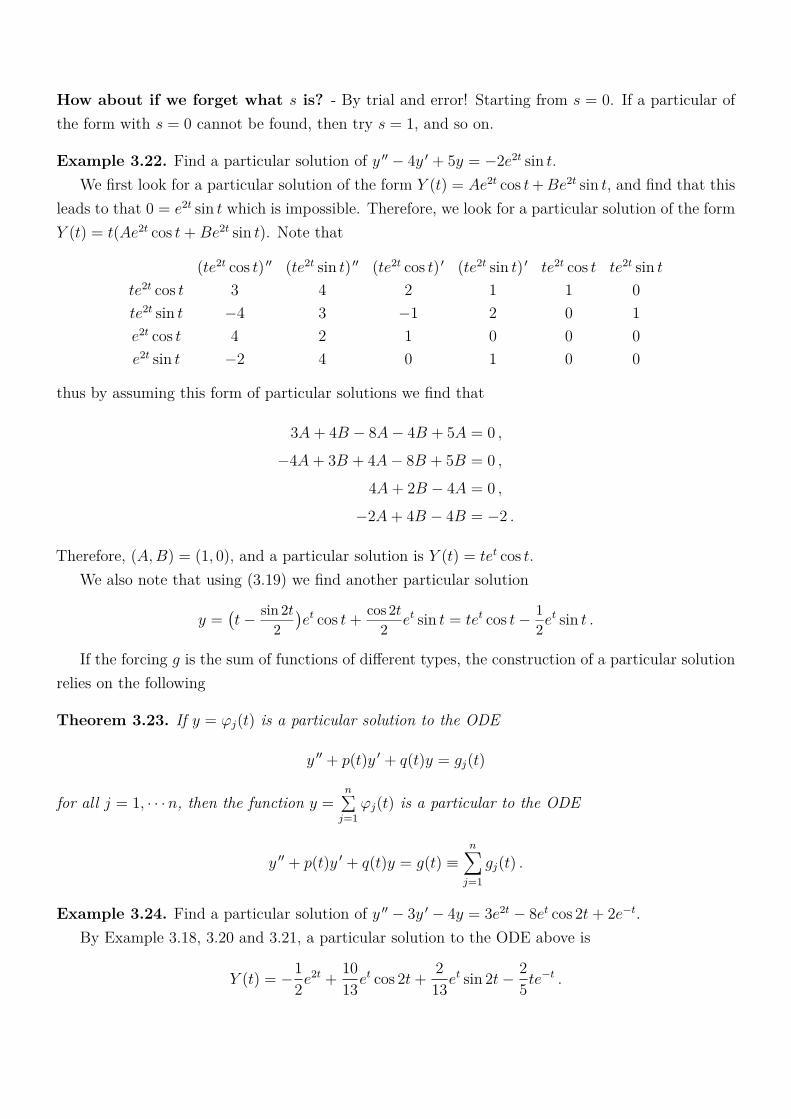
How about if we forget what s is? - By trial and error! Starting from s = 0. If a particular ofthe form with s = 0 cannot be found, then try s = 1, and so on.

Example 3.22. Find a particular solution of y 11 ´ 4y 1 + 5y = ´2e2t sin t.We first look for a particular solution of the form Y (t) = Ae2t cos t+Be2t sin t, and find that this

leads to that 0 = e2t sin t which is impossible. Therefore, we look for a particular solution of the formY (t) = t(Ae2t cos t+Be2t sin t). Note that

(te2t cos t) 11 (te2t sin t) 11 (te2t cos t) 1 (te2t sin t) 1 te2t cos t te2t sin tte2t cos t 3 4 2 1 1 0

te2t sin t ´4 3 ´1 2 0 1

e2t cos t 4 2 1 0 0 0

e2t sin t ´2 4 0 1 0 0

thus by assuming this form of particular solutions we find that

3A+ 4B ´ 8A ´ 4B + 5A = 0 ,

´4A+ 3B + 4A ´ 8B + 5B = 0 ,

4A+ 2B ´ 4A = 0 ,

´2A+ 4B ´ 4B = ´2 .

Therefore, (A,B) = (1, 0), and a particular solution is Y (t) = tet cos t.We also note that using (3.19) we find another particular solution

y =(t ´

sin 2t

2

)et cos t+ cos 2t

2et sin t = tet cos t ´

1

2et sin t .

If the forcing g is the sum of functions of different types, the construction of a particular solutionrelies on the following

Theorem 3.23. If y = φj(t) is a particular solution to the ODE

y 11 + p(t)y 1 + q(t)y = gj(t)

for all j = 1, ¨ ¨ ¨n, then the function y =nř

j=1

φj(t) is a particular to the ODE

y 11 + p(t)y 1 + q(t)y = g(t) ”

nÿ

j=1

gj(t) .

Example 3.24. Find a particular solution of y 11 ´ 3y 1 ´ 4y = 3e2t ´ 8et cos 2t+ 2e´t.By Example 3.18, 3.20 and 3.21, a particular solution to the ODE above is

Y (t) = ´1

2e2t +

10

13et cos 2t+ 2

13et sin 2t ´

2

5te´t .

3.6 Mechanical and Electrical Vibrations

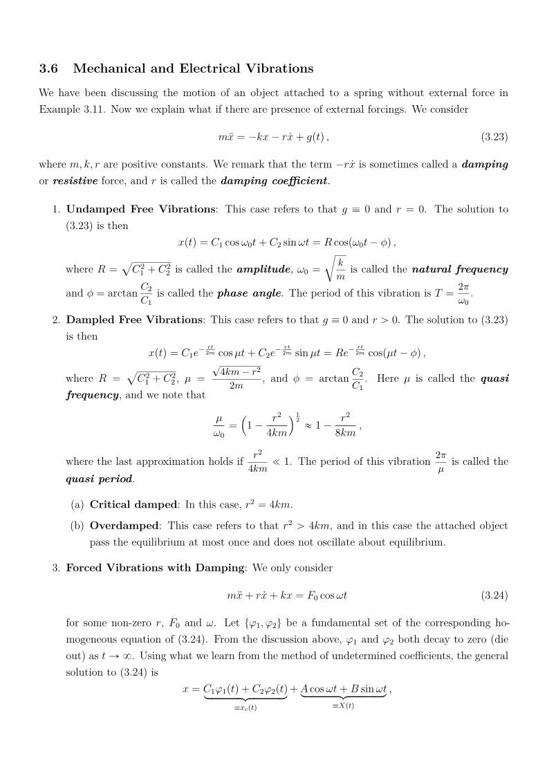
We have been discussing the motion of an object attached to a spring without external force inExample 3.11. Now we explain what if there are presence of external forcings. We consider

mx = ´kx ´ rx+ g(t) , (3.23)

where m, k, r are positive constants. We remark that the term ´rx is sometimes called a dampingor resistive force, and r is called the damping coefficient.

1. Undamped Free Vibrations: This case refers to that g ” 0 and r = 0. The solution to(3.23) is then

x(t) = C1 cosω0t+ C2 sinωt = R cos(ω0t ´ ϕ) ,

where R =a

C21 + C2

2 is called the amplitude, ω0 =

c

k

mis called the natural frequency

and ϕ = arctan C2

C1is called the phase angle. The period of this vibration is T =

2π

ω0.

2. Dampled Free Vibrations: This case refers to that g ” 0 and r ą 0. The solution to (3.23)is then

x(t) = C1e´ rt

2m cosµt+ C2e´ rt

2m sinµt = Re´ rt2m cos(µt ´ ϕ) ,

where R =a

C21 + C2

2 , µ =

?4km ´ r2

2m, and ϕ = arctan C2

C1. Here µ is called the quasi

frequency, and we note that

µ

ω0

=(1 ´

r2

4km

) 12

« 1 ´r2

8km,

where the last approximation holds if r2

4km! 1. The period of this vibration 2π

µis called the

quasi period.

(a) Critical damped: In this case, r2 = 4km.

(b) Overdamped: This case refers to that r2 ą 4km, and in this case the attached objectpass the equilibrium at most once and does not oscillate about equilibrium.

3. Forced Vibrations with Damping: We only consider

mx+ rx+ kx = F0 cosωt (3.24)

for some non-zero r, F0 and ω. Let tφ1, φ2u be a fundamental set of the corresponding ho-mogeneous equation of (3.24). From the discussion above, φ1 and φ2 both decay to zero (dieout) as t Ñ 8. Using what we learn from the method of undetermined coefficients, the generalsolution to (3.24) is

x = C1φ1(t) + C2φ2(t)loooooooooomoooooooooon

”xc(t)

+A cosωt+B sinωtloooooooooomoooooooooon

”X(t)

,

where C1 and C2 are chosen to satisfy the initial condition, and A and B are some constants sothat X(t) = A cosωt + B sinωt is a particular solution to (3.24). The part xc(t) is called thetransient solution and it decays to zero (die out) as t Ñ 8; thus as t Ñ 8, one sees thatonly a steady oscillation with the same frequency as the external force remains in the motion.x = X(t) is called the steady state solution or the forced response.

Since x = X(t) is a particular solution to (3.24), (A,B) satisfies

(k ´ ω2m)A+ rωB = F0 ,

´rωA+ (k ´ ω2m)B = 0 ;

thus with ω0 denoting the natural frequency; that is, ω0 =k

m, we have

(A,B) =(

F0m(ω20 ´ ω2)

m2(ω20 ´ ω2)2 + r2ω2

,F0rω

m2(ω20 ´ ω2)2 + r2ω2

).

Let α =ω

ω0, and Γ =

r2

mk. Then

(A,B) =F0

k

( 1 ´ α2

(1 ´ α2)2 + Γα2,

?Γα

(1 ´ α2)2 + Γα2

);

thusX(t) = R cos(ωt ´ ϕ) ,

where with ∆ denoting the numbera

(1 ´ α2)2 + Γα2, we have

R =?A2 +B2 =

F0

k∆and ϕ = arccos 1 ´ α2

∆.

Then if α ! 1, R «F0

kand ϕ « 0, while if α " 1, R ! 1 and ϕ « π.

In the intermediate region, some α, called αmax, maximize the amplitude R. Then αmax

minimize (1 ´ α2)2 + Γα2 which implies that αmax satisfies

α2max = 1 ´

Γ

2

and, when Γ ă 1, the corresponding maximum amplitude Rmax is

Rmax =F0

k

1?Γa

1 ´ Γ/4«

F0

k?Γ

(1 +

Γ

8

),

where the last approximation holds if Γ ! 1. If Γ ą 2, the maximum of R occurs at α = 0 (and

the maximum amplitude is Rmax =F0

k).

For lightly damped system; that is, r ! 1 (which implies that Γ ! 1), the maximum am-

plitude Rmax is closed to a very large number F0

k?Γ

. In this case αmax « 1, and this implies

that the frequency ωmax, where the maximum of R occurs, is very close to ω0. We call such aphenomena (that Rmax " 1 when ω « ω0) resonance. In such a case, αmax « 1; thus ϕ =

π

2which means the response occur π

2later than the peaks of the excitation.

4. Forced Vibrations without Damping:

(a) When r = 0, if ω ‰ ω0, then general solution to (3.24) is

x = C1 cosω0t+ C2 sinω0t+F0

m(ω20 ´ ω2)

cosωt ,

where C1 and C2 depends on the initial data. We are interested in the case that x(0) =x 1(0) = 0. In this case,

C1 = ´F0

m(ω20 ´ ω2)

and C2 = 0 ,

so the solution to (3.24) (with initial condition x(0) = x 1(0) = 0) is

x =F0

m(ω20 ´ ω2)

(cosωt ´ cosω0t

)=

2F0

m(ω20 ´ ω2)

sin ω0 ´ ω

2t sin ω0 + ω

2t .

When ω « ω0, R =2F0

m(ω20 ´ ω2)

sin ω0 ´ ω

2t presents a slowly varying sinusoidal amplitude.

This type of motion, possessing a periodic variation of amplitude, is called a beat.

(b) When r = 0 and ω = ω0, the general solution to (3.24) is

x = C1 cosω0t+ C2 sinω0t+F0

2mω0

t sinω0t .

4 Higher Order Linear Equations

4.1 General Theory of n-th Order Linear Equations

An n-th order linear ordinary differential equations is an equation of the form

Pn(t)dny

dtn+ Pn´1(t)

dn´1y

dtn´1+ ¨ ¨ ¨ + P1

dy

dt+ P0(t)y = G(t) ,

where Pn is never zero in the time interval of interest. Divide both sides by Pn(t), we obtain

L[y] =dny

dt+ pn´1(t)

dn´1y

dtn´1+ ¨ ¨ ¨ + p1(t)

dy

dt+ p0(t)y = g(t) . (4.1)

Suppose that pj ” 0 for all 0 ď j ď n ´ 1. Then to determine y, it requires n times integration andeach integration produce an arbitrary constant. Therefore, we expect that to determine the solutiony to (4.1) uniquely, it requires n initial conditions

y(t0) = y0, y 1(t0) = y1, ¨ ¨ ¨ , y(n´1)(t0) = yn´1 , (4.2)

where t0 is some point in an open interval I, and y0, y1, ¨ ¨ ¨ , yn´1 are some given constants.Equation (4.1) is called homogeneous if g ” 0.

Theorem 4.1. If the functions p0, ¨ ¨ ¨ , pn´1 and g are continuous on an open interval I, then thereexists exactly one solution y = φ(t) of the differential equation (4.1) with initial condition (4.2), wheret0 is any point in I. This solution exists throughout the interval I.

Definition 4.2. Let tφ1, ¨ ¨ ¨ , φnu be a collection of n differentiable functions defined on an openinterval I. The Wronskian of φ1, φ2, ¨ ¨ ¨ , φn at t0 P I, denoted by W (φ1, ¨ ¨ ¨ , φn)(t0), is the number

W (φ1, ¨ ¨ ¨ , φn)(t0) =

ˇ

ˇ

ˇ

ˇ

ˇ

ˇ

ˇ

ˇ

ˇ

ˇ

φ1(t0) φ2(t0) ¨ ¨ ¨ φn(t0)

φ 11(t0) φ 1

2(t0) ¨ ¨ ¨ φ 1n(t0)

... ... . . . ...φ(n´1)1 (t0) φ

(n´1)2 (t0) ¨ ¨ ¨ φ

(n´1)n (t0)

ˇ

ˇ

ˇ

ˇ

ˇ

ˇ

ˇ

ˇ

ˇ

ˇ

.

Theorem 4.3. Let y = φ1(t), y = φ2(t), ¨ ¨ ¨ , y = φn(t) be solutions to the homogeneous equation

L[y] =dny

dt+ pn´1(t)

dn´1y

dtn´1+ ¨ ¨ ¨ + p1(t)

dy

dt+ p0(t)y = 0 . (4.3)

Then the Wronskian of φ1, φ2, ¨ ¨ ¨ , φn satisfies

d

dtW (φ1, ¨ ¨ ¨ , φn)(t) + pn´1(t)W (φ1, ¨ ¨ ¨ , φn)(t) = 0 .

Proof. By the differentiation of the determinant, we find that

d

dtW (φ1, ¨ ¨ ¨ , φn) =

ˇ

ˇ

ˇ

ˇ

ˇ

ˇ

ˇ

ˇ

ˇ

ˇ

ˇ

ˇ

ˇ

φ1 φ2 ¨ ¨ ¨ φn

φ 11 φ 1

2(t0) ¨ ¨ ¨ φ 1n

... ... ...φ(n´2)1 φ

(n´2)2 ¨ ¨ ¨ φ

(n´2)n

φ(n)1 φ

(n)2 ¨ ¨ ¨ φ

(n)n

ˇ

ˇ

ˇ

ˇ

ˇ

ˇ

ˇ

ˇ

ˇ

ˇ

ˇ

ˇ

ˇ

=

ˇ

ˇ

ˇ

ˇ

ˇ

ˇ

ˇ

ˇ

ˇ

ˇ

ˇ

ˇ

ˇ

φ1 φ2 ¨ ¨ ¨ φn

φ 11 φ 1

2(t0) ¨ ¨ ¨ φ 1n

... ... ...φ(n´2)1 φ

(n´2)2 ¨ ¨ ¨ φ

(n´2)n

´pn´1φ(n´1)1 ´ ¨ ¨ ¨ ´ p0φ1 ´pn´1φ

(n´1)2 ´ ¨ ¨ ¨ ´ p0φ2 ¨ ¨ ¨ ´pn´1φ

(n´1)n ´ ¨ ¨ ¨ ´ p0φn

ˇ

ˇ

ˇ

ˇ

ˇ

ˇ

ˇ

ˇ

ˇ

ˇ

ˇ

ˇ

ˇ

= ´pn´1W (φ1, ¨ ¨ ¨ , φn) . ˝

Theorem 4.4. Suppose that the functions p0, ¨ ¨ ¨ , pn´1 are continuous on an open interval I. Ify = φ1(t), y = φ2(t), ¨ ¨ ¨ , y = φn(t) are solutions to the homogeneous equation (4.3) and theWronskian W (φ1, ¨ ¨ ¨ , φn)(t) ‰ 0 for at least one point t P I, then every solution of (4.3) can beexpressed as a linear combination of φ1, ¨ ¨ ¨ , φn.

Proof. Let y = φ(t) be a solution to (4.3), and suppose that W (φ1, ¨ ¨ ¨ , φn)(t0) ‰ 0. Define(y0, y1, ¨ ¨ ¨ , yn´1) =

(φ(t0), φ

1(t0), ¨ ¨ ¨ , φ(n´1)(t0)), and let C1, ¨ ¨ ¨ , Cn P R be the solution to

φ1(t0) φ2(t0) ¨ ¨ ¨ φn(t0)

φ 11(t0) φ 1

2(t0) ¨ ¨ ¨ φ 1n(t0)

... ... . . . ...φ(n´1)1 (t0) φ

(n´1)2 (t0) ¨ ¨ ¨ φ

(n´1)n (t0)

C1

C2

...Cn

=

y0

y1...

yn´1

.

We note that the system above has a unique solution since W (φ1, ¨ ¨ ¨ , φn)(t0) ‰ 0.Claim: φ(t) = C1φ1(t) + ¨ ¨ ¨ + Cnφn(t).Proof of Claim: Note that y = φ(t) and y = C1φ1(t) + ¨ ¨ ¨ + Cnφn(t) are both solutions to (4.3)satisfying the same initial condition. Therefore, by Theorem 4.1 the solution is unique, so the claimis concluded. ˝

Definition 4.5. A collection of solutions tφ1, ¨ ¨ ¨ , φnu to (4.3) is called a fundamental set of equation(4.3) if W (φ1, ¨ ¨ ¨ , φn)(t) ‰ 0 for some t in the interval of interest.

4.1.1 Linear Independence of Functions

Recall that in a vector space (V ,+, ¨) over scalar field F, a collection of vectors tv1, ¨ ¨ ¨ , vnu is calledlinearly dependent if there exist constants c1, ¨ ¨ ¨ , cn in F such that

nś

i=1

ci ” c1 ¨ c2 ¨ ¨ ¨ ¨ ¨ cn´1 ¨ cn ‰ 0

andc1 ¨ v1 + ¨ ¨ ¨ + cn ¨ vn = 0 .

If no such c1, ¨ ¨ ¨ , cn exists, tv1, ¨ ¨ ¨ , vnu is called linearly independent. In other words, tv1, ¨ ¨ ¨ , vnu Ď

V is linearly independent if and only if

c1 ¨ v1 + ¨ ¨ ¨ + cn ¨ vn = 0 ô c1 = c2 = ¨ ¨ ¨ = cn = 0 .

Now let V denote the collection of all (n ´ 1)-times differentiable functions defined on an openinterval I. Then (V ,+, ¨) clearly is a vector space over R. Given tf1, ¨ ¨ ¨ , fnu Ď V, we would like todetermine the linear dependence or independence of the n-functions tf1, ¨ ¨ ¨ , fnu. Suppose that

c1f1(t) + ¨ ¨ ¨ + cnfn(t) = 0 @ t P I .

Since each fj are (n ´ 1)-times differentiable, we have for 1 ď k ď n ´ 1,

c1f(k)1 (t) + ¨ ¨ ¨ + cnf

(k)n (t) = 0 @ t P I .

In other words, c1, ¨ ¨ ¨ , cn satisfyf1(t) f2(t) ¨ ¨ ¨ fn(t)f 11(t) f 1

2(t) ¨ ¨ ¨ f 1n(t)

... ...f(n´1)1 (t) f

(n´1)2 (t) ¨ ¨ ¨ f

(n´1)n (t)

c1c2...cn

=

00...0

@ t P I .

If there exists t0 P I such that the matrix

f1(t0) f2(t0) ¨ ¨ ¨ fn(t0)f 11(t0) f 1

2(t0) ¨ ¨ ¨ f 1n(t0)

... ...f(n´1)1 (t0) f

(n´1)2 (t0) ¨ ¨ ¨ f

(n´1)n (t0)

is non-singular,

then c1 = c2 = ¨ ¨ ¨ = cn = 0. Therefore, a collection of solutions tφ1, ¨ ¨ ¨ , φnu is a fundamental set ofequation (4.3) if and only if tφ1, ¨ ¨ ¨ , φnu is linearly independent.

4.1.2 The Homogeneous Equations - Reduction of Orders

Suppose that y = φ1(t) is a solution to (4.3). Now we look for a function v such that y = v(t)φ1(t) isalso a solution to (4.3). The derivative of this v satisfies an (n ´ 1)-th order homogeneous ordinarydifferential equation.

Example 4.6. Suppose that we are given y = φ1(t) = et as a solution to

(2 ´ t)y 12 + (2t ´ 3)y 11 ´ ty 1 + y = 0 for t ă 2 . (4.4)

Suppose that y = v(t)et is also a solution to (4.4). Then

(2 ´ t)(v 12et + 3v 11et + 3v 1et + vet) + (2t ´ 3)(v 11et + 2v 1et + vet) ´ t(v 1et + vet) + vet = 0

which implies that v satisfies

(2 ´ t)v 12 +[3(2 ´ t) + (2t ´ 3)

]v 11 +

[3(2 ´ t) + 2(2t ´ 3) ´ t

]v 1 = 0

or equivalently, with u denoting v 11,

(2 ´ t)u 1 + (3 ´ t)u = 0 .

Solving the ODE above, we find that u(t) = C1(2 ´ t)e´t for some constant C1; thus

v(t) = C3 + C2t+ C1e´t ´ C1(t+ 1)e´t = C3 + C2t ´ C1te

´t .

Therefore, a fundamental set of (4.4) is tet, tet, tu.

4.1.3 The Nonhomogeneous Equations

Let y = Y1(t) and y = Y2(t) be solutions to (4.1). Then y = Y1(t) ´ Y2(t) is a solution to thehomogeneous equation (4.3); thus if tφ1, ¨ ¨ ¨ , φnu is a fundamental set of (4.3), then

Y1(t) ´ Y2(t) = C1φ1(t) + ¨ ¨ ¨ + Cnφn(t) .

Therefore, we establish the following theorem which is similar to Theorem 3.14.

Theorem 4.7. The general solution of the nonhomogeneous equation (4.1) can be written in theform

y = φ(t) = C1φ1(t) + C2φ2(t) + ¨ ¨ ¨ + Cnφn(t) + Y (t) ,

where tφ1, ¨ ¨ ¨ , φnu is a fundamental set of (4.3), C1, ¨ ¨ ¨ , Cn are arbitrary constants, and y = Y (t)

is a particular solution of the nonhomogeneous equation (4.1).

In general, in order to solve (4.1), we follow the procedure listed below:

1. Find the space of complementary solution to (4.3); that is, find the general solution y =

C1φ1(t) + C2φ2(t) + ¨ ¨ ¨ + Cnφn of the homogeneous equation (4.3).

2. Find a particular solution y = Y (t) of the nonhomogeneous equation (4.1).

3. Apply Theorem 4.7.

4.2 Homogeneous Equations with Constant Coefficients

We now consider the n-th order linear homogeneous ODE with constant coefficients

L[y] = y(n) + an´1y(n´1) + ¨ ¨ ¨ + a1y

1 + a0y = 0 , (4.5)

where aj’s are constants for all j P t0, 1, ¨ ¨ ¨ , n ´ 1u. Suppose that r1, r2, ¨ ¨ ¨ , rn are solutions to thecharacteristic equation of (4.5)

rn + an´1rn´1 + ¨ ¨ ¨ + a1r + a0 = 0 .

Then (4.5) can be written as ( ddt

´ r1

)( ddt

´ r2

)¨ ¨ ¨

( ddt

´ rn

)y = 0

1. If the characteristic equation of (4.5) has distinct roots, then

y(t) = C1er1t + C2e

r2t + ¨ ¨ ¨ + Cnernt . (4.6)

Reason: Let z1 =( d

dt´ r2

)¨ ¨ ¨

( d

dt´ rn

)y. Then z 1

1 ´ r1z1 = 0; thus z1(t) = c1er1t.

Let z2 =( d

dt´ r3

)¨ ¨ ¨

( d

dt´ rn

)y. Then z 1

2 ´ r2z2 = c1z1; thus using the method of integrating

factors, we find that

d

dt

(e´r2tz2

)= c1e

(r1´r2)t ñ z2(t) =c1

r1 ´ r2er1t + c2e

r2t . (4.7)

Repeating the process, we conclude (4.6).

How about if there are complex roots? Suppose that r1 = a + bi and r2 = a ´ bi, thenthe Euler identity implies that, by choosing complex c1 and c2 in (4.7), we find that

z2(t) = c1eat cos bt+ c2e

at sin bt

for some constants c1 and c2. Therefore, suppose that we have complex roots ak ˘ bki fork = 1, ¨ ¨ ¨ , ℓ and real roots r2ℓ+1, ¨ ¨ ¨ , rn. Then the general solution to (4.6) is

y(t) = C1ea1t cos b1t+ C2e

a1t sin b1t+ ¨ ¨ ¨ + C2ℓ´1eaℓt cos bℓt+ C2ℓe

aℓt sin bℓt+ C2ℓ+1e

r2ℓ+1t + ¨ ¨ ¨ + Cnernt .

2. If the characteristic equation of (4.5) has repeated roots, we group the roots in such a way thatr1 = r2 = ¨ ¨ ¨ = rℓ and so on; that is, repeated roots appear in a successive order. Then theimplication in (4.7) is modified to

d

dt

(e´r2tz2

)= c1e

(r1´r2)t = c1 ñ z2(t) = (c1t+ c2)er1t .

(a) Suppose that r3 = r2 = r1 = r. Letting z3 =( d

dt´ r4

)¨ ¨ ¨

( d

dt´ rn

)y, we find that

z 13 ´ rz3 = (c1t+ c2)e

rt ;

thus the method of integrating factor implies that

d

dt

(e´rtz3

)= c1t+ c2 ñ z3(t) =

(c12t2 + c2t+ c3)e

rt .

(b) Suppose that r1 = r2 = r and r3 ‰ r2. Letting z3 =( d

dt´ r4

)¨ ¨ ¨

( d

dt´ rn

)y, we find that

z 13 ´ r3z3 = (c1t+ c2)e

rt ;

thus the method of integrating factor implies that

d

dt

(e´r3tz3

)= (c1t+ c2)e

(r´r3)t ñ z3(t) =(rc1t+ rc2)e

rt + c3er3t .

From the discussion above, we “conjecture” that if rj’s are roots of the characteristic equation of(4.5) with multiplicity nj (so that n1 + ¨ ¨ ¨ + nk = n), then the general solution to (4.5) is

y(t) =kÿ

j=1

pj(t)erjt ,

where pj(t)’s are some polynomials of degree nj ´ 1. Note that in each pj there are nj constants tobe determined by the initial conditions.

If there are repeated complex roots, say r1 = a+ bi and r2 = a´ bi with n1 = n2. Then p1 and p2are polynomials of degree n1; thus by adjusting constants in the polynomials properly, we find that

p1(t)er1t + p2(t)e

r2t = rp1(t)eat cos bt+ rp2(t)e

at sin bt .

In other words, if rj are real roots of the characteristic equation of (4.5) with multiplicity nj andak ˘ ibk are complex roots of the characteristic equation of (4.5) with multiplicity mk (so thatř

j

nj +ř

k

2mk = n), then the general solution to (4.5) is

y(t) =ÿ

j

pj(t)erjt +

ÿ

k

eakt(q1k(t) cos bkt+ q2k(t) sin bkt

),

where pj(t)’s are some polynomials of degree nj ´1 and q1k, q2k’s are some polynomials of degree mk´1.

Example 4.8. Find the general solution of

y(4) + y 12 ´ 7y 11 ´ y 1 + 6y = 0 .

The roots of the characteristic equation is r = ˘1, r = 2 and r = ´3; thus the general solution tothe ODE above is

y = C1et + C2e

´t + C3e2t + C4e

´3t .

If we are looking for a solution to the ODE above satisfying the initial conditions y(0) = 1, y 1(0) = 0,y 11(0) = ´1 and y 12(0) = ´1, then C1, C2, C3, C4 have to satisfy

1 1 1 11 ´1 2 ´31 1 4 91 ´1 8 ´27

C1

C2

C3

C4

=

10

´1´1

.

Solving the linear system above, we find that the solution solving the ODE with the given initialdata is

y =11

8et +

5

12e´t ´

2

3e2t ´

1

8e´3t .

Example 4.9. Find the general solution of

y(4) ´ y = 0 .

Also find the solution that satisfies the initial condition

y(0) =7

2, y 1(0) = ´4 , y 11(0) =

5

2, y 12(0) = ´2 .

The roots of the characteristic equation are r = ˘1 and r = ˘i. Therefore, the general solutionto the ODE above is

y = C1et + C2e

´t + C3 cos t+ C4 sin t .

To satisfy the initial condition, C1, ¨ ¨ ¨ , C4 has to satisfy

1 1 1 01 ´1 0 11 1 ´1 01 ´1 0 ´1

C1

C2

C3

C4

=

7

2´45

2´2

.

Solving the linear system above, we find that the solution solving the ODE with the given initialdata is

y = 3e´t +1

2cos t ´ sin t .

Example 4.10. Find the general solution of

y(4) + y = 0 .

The roots of the characteristic equation are r = ˘(?

2

2˘

?2

2i). Therefore, the general solution

to the ODE above is

y = exp(?

2

2t)(C1 cos

?2

2t+ C2 sin

?2

2t)+ exp

(´

?2

2t)(C2 cos

?2

2t+ C4 sin

?2

2t).

4.3 The Method of Variation of Parameters

To solve a non-homogeneous ODE

L[y] =dny

dt+ pn´1(t)

dn´1y

dtn´1+ ¨ ¨ ¨ + p1(t)

dy

dt+ p0(t)y = g(t) , (4.1)

often times we apply the method of variation of parameters to find a particular solution. Suppose thattφ1, ¨ ¨ ¨ , φnu is a fundamental set of the homogeneous equation (4.3), we assume that a particularsolution can be written as

y = Y (t) = u1(t)φ1(t) + ¨ ¨ ¨ + un(t)φn(t) .

Assume that u1, ¨ ¨ ¨ , un satisfyu 11φ

(j)1 + ¨ ¨ ¨ + u 1

nφ(j)n = 0

for j = 0, ¨ ¨ ¨ , 1, n ´ 2. Then

Y 1 = u1φ11 + ¨ ¨ ¨ + unφ

1n ,

Y 11 = u1φ111 + ¨ ¨ ¨ + unφ

11n ,

...

Y (n´1) = u1φ(n´1)1 + ¨ ¨ ¨ + unφ

(n´1)n ,

andY (n) = u 1

1φ(n´1)1 + ¨ ¨ ¨ + u 1

nφ(n´1)n + u1φ

(n)1 + ¨ ¨ ¨ + unφ

(n)n .

Since y = Y (t) is assumed to be a particular solution of (4.1), we have

u 11φ

(n´1)1 + ¨ ¨ ¨ + u 1

nφ(n´1)n = g(t) .

Therefore, u1, ¨ ¨ ¨ , un satisfyφ1 φ2 ¨ ¨ ¨ φn

φ 11 φ 1

2 ¨ ¨ ¨ φ 1n

... . . . ...φ(n´1)1 φ

(n´1)2 ¨ ¨ ¨ φ

(n´1)n

u 11

u 12...u 1n

=

0...0g

.

Let Wm denote the Wronskian of tφ1, ¨ ¨ ¨ , φm´1, φm+1, ¨ ¨ ¨ , φnu; that is,

Wm =

ˇ

ˇ

ˇ

ˇ

ˇ

ˇ

ˇ

ˇ

ˇ

φ1 ¨ ¨ ¨ φm´1 φm+1 ¨ ¨ ¨ φn

φ 11 ¨ ¨ ¨ φ 1

m´1 φ 1m+1 ¨ ¨ ¨ φ 1

n... ... ... ...

φ(n´2)i ¨ ¨ ¨ φ

(n´2)m´1 φ

(n´2)m+1 ¨ ¨ ¨ φ

(n´2)n

ˇ

ˇ

ˇ

ˇ

ˇ

ˇ

ˇ

ˇ

ˇ

.

Then u 1i = (´1)n+i Wi

W (φ1, ¨ ¨ ¨ , φn)which implies that

Y (t) =nÿ

i=1

(´1)n+iφi(t)

ż t

t0

Wi(s)g(s)

W (φ1, ¨ ¨ ¨ , φn)(s)ds .

Example 4.11. Find the general solution to

y 12 ´ y 11 ´ y 1 + y = g(t) . (4.8)

Note the the roots of the characteristic equation r3 ´ r2 ´ r+1 = 0 of the homogeneous equation

y 12 ´ y 11 ´ y 1 + y = 0 (4.9)

are r = 1 (double) and r = ´1; thus we have a fundamental set tet, tet, e´tu of equation (4.9). Letφ1(t) = et, φ2(t) = tet and φ3(t) = e´t. Then

W (φ1, φ2, φ3)(t) =

ˇ

ˇ

ˇ

ˇ

ˇ

ˇ

et tet e´t

et (t+ 1)et ´e´t

et (t+ 2)et e´t

ˇ

ˇ

ˇ

ˇ

ˇ

ˇ

=[(t+ 1) + (t+ 2) ´ t ´ (t+ 1) ´ t+ (t+ 2)

]et = 4et ,

and W1(t) = ´2t ´ 1, W2(t) = ´2 and W3(t) = e2t. Therefore, a particular solution is

Y (t) = etż t

0

(´2s ´ 1)

4esg(s)ds ´ tet

ż s

0

´2

4esg(s)ds+ e´t

ż t

0

e2s

4esg(s)ds

=1

4

ż t

0

[2(t ´ s) ´ 1)et´s + es´t

]g(s)ds ,

and the general solution to (4.8) is

y = C1et + C2te

t + C3e´t + Y (t) .

5 Series Solutions of Second Order Linear Equations

5.1 Properties of Power Series

Definition 5.1. A power series about c is a series of the form8ř

k=0

ak(x ´ c)k for some sequence

taku8k=0 Ď R (or C) and c P R (or C).

Proposition 5.2. If a power series centered at c is convergent at some point b ‰ c, then the powerseries converges absolutely for all points in (c ´ |b ´ c|, c+ |b ´ c|).

Proof. Since the series8ř

k=0

ak(b ´ c)k converges, |ak||b ´ c|k Ñ 0 as k Ñ 8; thus there exists M ą 0

such that |ak||b ´ c|k ď M for all k. Then if x P (c ´ |b ´ c|, c + |b ´ c|), the series8ř

k=0

ak(x ´ c)k

converges absolutely since8ÿ

k=0

|ak(x ´ c)k| =8ÿ

k=0

|ak||x ´ c|k =8ÿ

k=0

|ak||b ´ c|k|x ´ c|k

|b ´ c|kď M

8ÿ

k=0

( |x ´ c|

|b ´ c|

)k

which converges (because of the geometric series test or ratio test). ˝

Definition 5.3. A number R is called the radius of convergence of the power series8ř

k=0

ak(x´c)k

if the series converges for all x P (c ´ R, c + R) but diverges if x ą c + R or x ă c ´ R. In otherwords,

R = sup

r ě 0ˇ

ˇ

8ÿ

k=0

ak(x ´ c)k converges in [c ´ r, c+ r](

.

The interval of convergence or convergence interval of a power series is the collection of allx at which the power series converges.

We remark that Proposition 5.2 implies that a power series converges absolutely in the interiorof the interval of convergence.

Proposition 5.4. A power series is continuous in the interior of the convergence interval; that is, ifR ą 0 is the radius of convergence of the power series

8ř

k=0

ak(x´c)k, then8ř

k=0

ak(x´c)k is continuous

in (c ´ R, c+R).

Proof. W.L.O.G., we prove that the power series is continuous at x0 P [c, c+R). Let ε ą 0 be given.

Define r = c+R ´ x02

. Then |r| ă R; thus there exists N ą 0 such that8ÿ

k=N+1

|ak|rk ăε

4.

Moreover, sinceNř

k=0

ak(x ´ c)k is continuous at x0, there exists 0 ă δ ă r such that

ˇ

ˇ

ˇ

Nÿ

k=0

ak(x ´ c)k ´

Nÿ

k=0

ak(x0 ´ c)kˇ

ˇ

ˇăε

2@ |x ´ x0| ă δ .

Therefore, if |x ´ x0| ă δ, we have

ˇ

ˇ

ˇ

8ÿ

k=0

ak(x ´ c)k ´

8ÿ

k=0

ak(x0 ´ c)kˇ

ˇ

ˇ

ď

ˇ

ˇ

ˇ

Nÿ

k=0

ak(x ´ c)k ´

Nÿ

k=0

ak(x0 ´ c)kˇ

ˇ

ˇ+

8ÿ

k=N+1

|ak|rk|x ´ c|k

rk+

8ÿ

k=N+1

|ak|rk|x0 ´ c|k

rk

ď

ˇ

ˇ

ˇ

Nÿ

k=0

ak(x ´ c)k ´

Nÿ

k=0

ak(x0 ´ c)kˇ

ˇ

ˇ+ 2

8ÿ

k=N+1

|ak|rk ă ε

which implies that8ř

k=0

ak(x ´ c)k is continuous at x0. ˝

Theorem 5.5. Let R ą 0 be the radius of convergence of the power series8ř

k=0

ak(x ´ c)k. Then

ż x

c

8ÿ

k=0

ak(t ´ c)kdt =8ÿ

k=0

akk + 1

(x ´ c)k+1 @x P (c ´ R, c+R) .

Proof. W.L.O.G., we assume that x P (c, c+R). Let ε ą 0 be given. Choose x0 P (c´R, c+R) suchthat |x ´ c| ă |x0 ´ c|. Then for t P [c, x], |t ´ c|

|x0 ´ c|ď 1. Moreover, since

8ř

k=1

ak(x0 ´ c)k converges

absolutely, there exists N ě 0 such that8ÿ

k=N+1

|ak||x0 ´ c|k ďε

|x0 ´ c|.

Sinceż x

c

8ÿ

k=0

ak(t ´ c)kdt =

ż x

c

nÿ

k=0

ak(t ´ c)kdt+

ż x

c

8ÿ

k=N+1

ak(t ´ c)kdt

=nÿ

k=0

akk + 1

(x ´ c)k+1 +

ż x

c

8ÿ

k=n+1

ak(t ´ c)kdt ,

we have for n ě N ,

ˇ

ˇ

ˇ

ż x

c

8ÿ

k=0

ak(t ´ c)kdt ´

nÿ

k=0

akk + 1

(x ´ c)k+1ˇ

ˇ

ˇď

ż x

c

8ÿ

k=n+1

|ak||x0 ´ c|k(t ´ c)k

|x0 ´ c|kdt

ď

ż x

c

8ÿ

k=N+1

|ak||x0 ´ c|kdt ď |x0 ´ c|8ÿ

k=N+1

|ak||x0 ´ c|k ă ε .

In other words, limnÑ8

nř

k=0

akk + 1

(x ´ c)k+1 =ż x

c

8ř

k=0

ak(t ´ c)kdt which concludes the corollary. ˝

Theorem 5.6. Let R ą 0 be the radius of convergence of the power series8ř

k=0

ak(x ´ c)k. Then

d

dx

8ÿ

k=0

ak(x ´ c)k =8ÿ

k=1

kak(x ´ c)k´1 @ x P (c ´ R, c+R) .

Proof. We first show that the series8ř

k=1

kak(x ´ c)k´1 also converges for all x P (c ´ R, c + R). Let

x P (c ´ R, c+R). Then there exists x0 P (c ´ R, c+R) such that |x ´ c| ă |x0 ´ c|. Choose N ą 0

such thatk

|x ´ c|k

|x0 ´ c|kď 1 if k ě N .

We note that it is possible to find such an N since limkÑ8

k|x ´ c|k

|x0 ´ c|k= 0. Therefore,

8ÿ

k=0

k|ak||x ´ c|k =Nÿ

k=0

k|ak||x ´ c|k +8ÿ

k=N+1

k|ak||x ´ c|k

ď

Nÿ

k=0

k|ak||x ´ c|k +8ÿ

k=N+1

|ak||x0 ´ c|kk|x ´ c|k

|x0 ´ c|k

ď

Nÿ

k=0

k|ak||x ´ c|k +8ÿ

k=N+1

|ak||x0 ´ c|k ă 8

which implies that the series8ř

k=0

k|ak||x ´ c|k converges absolutely.

Now, Theorem 5.5 implies thatż x

c

8ÿ

k=1

kak(t ´ c)k´1dt =

ż x

c

8ÿ

k=0

(k + 1)ak+1(t ´ c)kdt =8ÿ

k=0

ak+1(x ´ c)k+1 =8ÿ

k=1

ak(x ´ c)k ;

thus we havea0 +

ż x

c

8ÿ

k=1

kak(t ´ c)k´1dt =8ÿ

k=0

ak(x ´ c)k .

Moreover, Proposition 5.4 implies that the power series8ř

k=0

k|ak||x´c|k is continuous in (c´R, c+R).

As a consequence, the fundamental theorem of Calculus implies that8ÿ

k=1

kak(x ´ c)k´1 =d

dx

ż x

c

8ÿ

k=1

kak(t ´ c)k´1dt =d

dx

8ÿ

k=0

ak(x ´ c)k

which concludes the theorem. ˝

Definition 5.7. A function f : (a, b) Ñ R is said to be analytic at c P (a, b) if f is infinitely manytimes differentiable at c and there exists R ą 0 such that

f(x) =8ÿ

k=0

ak(x ´ c)k @ x P (c ´ R, c+R) Ď (a, b)

for some sequence taku8k=0.

Remark 5.8. If f : (a, b) Ñ R is analytic at c P (a, b), then Theorem 5.6 implies that

f(x) =8ÿ

k=0

f (k)(c)

k!(x ´ c)k @ x P (c ´ R, c+R) Ď (a, b)

for some R ą 0.A function which is infinitely many times differentiable at a point c might not be analytic at c.

For example, consider the function

f(x) =

#

exp(

´1

x2

)if x ‰ 0 ,

0 if x = 0 .

Then f (k)(0) = 0 for all k P N which implies that f cannot be analytic at 0.

5.1.1 Product of Power Series

Definition 5.9. Given two series8ř

n=0

an and8ř

n=0

bn, the series8ř

n=0

cn, where cn =nř

k=0

akbn´k for all

n P N Y t0u, is called the Cauchy product of8ř

n=0

an and8ř

n=0

bn.

Theorem 5.10. Suppose that the two series8ř

n=0

an and8ř

n=0

bn converge absolutely. Then the Cauchy

product of8ř

n=0

an and8ř

n=0

bn converges absolutely to( 8ř

n=0

an

)( 8ř

n=0

bn

); that is,

8ÿ

n=0

( nÿ

k=0

akbn´k

)=

( 8ÿ

n=0

an

)( 8ÿ

n=0

bn

).

Proof. Claim: If8ř

n=0

an converges absolutely and π : N Ñ N is bijective (that is, one-to-one and

onto), then8ř

n=0

aπ(n) converges absolutely to8ř

n=0

an.

Proof of claim: Let8ř

n=0

an = a and ε ą 0 be given. Since8ř

n=0

an converges absolutely, there exists

N ą 0 such that 8ÿ

n=N+1

|an| ăε

2.

Let K = max

π´1(1), ¨ ¨ ¨ , π´1(N)(

+ 1. Then if k ě K, π(k) ě N + 1; thus if k ě K,8ÿ

n=k+1

|aπ(n)| ď

8ÿ

n=N+1

|an| ăε

2

andˇ

ˇ

ˇ

kÿ

n=0

aπ(n) ´ aˇ

ˇ

ˇď

ˇ

ˇ

ˇ

kÿ

n=0

aπ(n) ´

Nÿ

n=0

an

ˇ

ˇ

ˇ+ˇ

ˇ

ˇ

Nÿ

n=0

an ´ aˇ

ˇ

ˇď 2

8ÿ

n=N+1

|an| ă ε .

Therefore,8ř

n=0

aπ(n) converges absolutely to a.

Claim: If8ř

n=0

an and8ř

n=0

bn converge absolutely, then8ř

n,m=1

anbm converges absolutely and

8ÿ

n,m=1

anbm =( 8ÿ

n=1

an

)( 8ÿ

m=1

bm

),

where8ř

n,m=1

anbm denotes the limit limN,MÑ8

Nř

n=1

Mř

m=1

anbm.

Proof of claim: If N1 ă N2 and M1 ă M2,ˇ

ˇ

ˇ

( N1ÿ

n=1

an

)( M1ÿ

m=0

bm

)´

( N2ÿ

n=1

an

)( M2ÿ

m=0

bm

)ˇˇ

ˇď

N1ÿ

n=1

|an|

M2ÿ

m=M1+1

|bm| +N2ÿ

n=N1+1

|an|

M2ÿ

m=1

|bm|

thusˇ

ˇ

ˇ

( N1ÿ

n=1

an

)( M1ÿ

m=0

bm

)´

8ÿ

n,m=1

anbm

ˇ

ˇ

ˇ

= limN2,M2Ñ8

ˇ

ˇ

ˇ

( N1ÿ

n=1

an

)( M1ÿ

m=0

bm

)´

( N2ÿ

n=1

an

)( M2ÿ

m=0

bm

)ˇˇ

ˇ

ď

( 8ÿ

n=1

|an| +8ÿ

m=1

|bm|

)( 8ÿ

n=N1+1

|an| +8ÿ

m=M1+1

|bm|

).

The claim is then concluded by passing to the limit as M1 Ñ 8 and then N1 Ñ 8.The theorem follows from the fact that the Cauchy product is a special rearrangement of the

series8ř

n,m=1

anbm. ˝

Corollary 5.11. Let R1, R2 ą 0 be the radius of convergence of the power series8ř

k=0

ak(x ´ c)k and8ř

k=0

bk(x ´ c)k, respectively. Then with R denoting mintR1, R2u, we have

( 8ÿ

k=0

ak(x ´ c)k)( 8

ÿ

k=0

bk(x ´ c)k)=

8ÿ

n=0

( nÿ

k=0

akbn´k

)(x ´ c)n @ x P (c ´ R, c+R) .

5.1.2 General Theory

The discussion of the power series is for the purpose of solving ODE with analytic coefficients andforcings.

Theorem 5.12 (Cauchy-Kowalevski, Special case). Let Ω Ď Rn be an open set, and f : Ω ˆ (t0 ´

h, t0 + h) Ñ Rn be an analytic function in some neighborhood (x0, t0) for some x0 P Ω; that is, forsome r ą 0,

f(y, t) = f(y0, t0) +8ÿ

k=1

ÿ

|α|+j=k

cα,j(y ´ y0)α(t ´ t0)

j @ (y, t) P B((y0, t0), r

),

where α = (α1, ¨ ¨ ¨ , αn) is a multi-index satisfying yα = yα11 ¨ ¨ ¨ yαn

n and |α| = α1 + ¨ ¨ ¨αn. Then thereexists 0 ă δ ă h such that the ODE y 1(t) = f(y, t) with initial condition y(t0) = y0 has a uniqueanalytic solution in the interval (t0 ´ δ, t0 + δ).

Remark 5.13. If f is continuous at (y0 ´ k, y0 + k) ˆ (t0 ´ h, t0 + h), then the general existenceand uniqueness theorem guarantees the existence of a unique solution of y 1(t) = f(y, t) with initialcondition y(t0) = y0 in some time interval (t0 ´ δ, t0 + δ). Theorem 5.12 further implies that thesolution is analytic if the “forcing” function f is analytic.

5.2 Series Solutions Near an Ordinary Point: Part I

In the remaining chapter we focus on the second order linear homogeneous ODE

P (x)d2y

dx2+Q(x)

dy

dx+R(x)y = 0 , (5.1)

where P,Q,R are assumed to have no common factors. We note that we change the independentvariable from t to x.

Definition 5.14. A point x0 is said to be a ordinary point to ODE (5.1) if P (x0) ‰ 0, and thetwo functions Q/P , R/P are analytic at x0. It is called a singluar point if it is not a regular point.It is called a regular singular point if the two limits

limxÑx0

(x ´ x0)Q(x)

P (x)and lim

xÑx0

(x ´ x0)2R(x)

P (x)

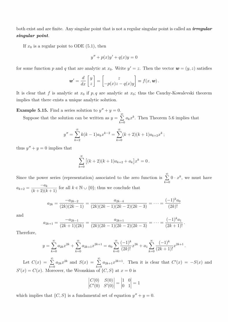
both exist and are finite. Any singular point that is not a regular singular point is called an irregularsingular point.

If x0 is a regular point to ODE (5.1), then

y 11 + p(x)y 1 + q(x)y = 0

for some function p and q that are analytic at x0. Write y 1 = z. Then the vector w = (y, z) satisfies

w 1 =d

dx

[yz

]=

[z

´p(x)z ´ q(x)y

]” f(x,w) .

It is clear that f is analytic at x0 if p, q are analytic at x0; thus the Cauchy-Kowalevski theoremimplies that there exists a unique analytic solution.

Example 5.15. Find a series solution to y 11 + y = 0.Suppose that the solution can be written as y =

8ř

k=0

akxk. Then Theorem 5.6 implies that

y 11 =8ÿ

k=2

k(k ´ 1)akxk´2 =

8ÿ

k=0

(k + 2)(k + 1)ak+2xk ;

thus y 11 + y = 0 implies that8ÿ

k=0

[(k + 2)(k + 1)ak+2 + ak

]xk = 0 .

Since the power series (representation) associated to the zero function is8ř

k=0

0 ¨ xk, we must have

ak+2 =´ak

(k + 2)(k + 1)for all k P N Y t0u; thus we conclude that

a2k =´a2k´2

(2k)(2k ´ 1)=

a2k´4

(2k)(2k ´ 1)(2k ´ 2)(2k ´ 3)= ¨ ¨ ¨ =

(´1)ka0(2k)!

anda2k+1 =

´a2k´1

(2k + 1)(2k)=

a2k+1

(2k)(2k ´ 1)(2k ´ 2)(2k ´ 3)= ¨ ¨ ¨ =

(´1)ka1(2k + 1)!

.

Therefore,

y =8ÿ

k=0

a2kx2k +

8ÿ

k=0

a2k+1x2k+1 = a0

8ÿ

k=0

(´1)k

(2k)!x2k + a1

8ÿ

k=0

(´1)k

(2k + 1)!x2k+1 .

Let C(x) =8ř

k=0

a2kx2k and S(x) =

8ř

k=0

a2k+1x2k+1. Then it is clear that C 1(x) = ´S(x) and

S 1(x) = C(x). Moreover, the Wronskian of tC, Su at x = 0 isˇ

ˇ

ˇ

ˇ

C(0) S(0)C 1(0) S 1(0)

ˇ

ˇ

ˇ

ˇ

=

ˇ

ˇ

ˇ

ˇ

1 00 1

ˇ

ˇ

ˇ

ˇ

= 1

which implies that tC, Su is a fundamental set of equation y 11 + y = 0.

Example 5.16. Find a series solution to Airy’s equation y 11 ´ xy = 0.Suppose that the solution can be written as y =

8ř

k=0

akxk. Then

y 11 =8ÿ

k=2

k(k ´ 1)akxk´2 =

8ÿ

k=0

(k + 2)(k + 1)ak+2xk ;

andxy =

8ÿ

k=0

akxk+1 =

8ÿ

k=1

ak´1xk .

Therefore,

a2 +8ÿ

k=1

[(k + 2)(k + 1)ak+2 ´ ak´1

]xk = 0

which implies that a2 = 0 and ak+2 =ak´1

(k + 2)(k + 1)for all k P N. The recurrence relation further

implies that a5 = a8 = a11 = ¨ ¨ ¨ = a3k´1 = ¨ ¨ ¨ = 0 for all k P N. Furthermore, we have

a3k =a3k´3

(3k)(3k ´ 1)=

a3k´6

(3k)(3k ´ 1)(3k ´ 3)(3k ´ 4)= ¨ ¨ ¨

=a0

(3k)(3k ´ 1)(3k ´ 3)(3k ´ 4) ¨ ¨ ¨ 3 ¨ 2=

(3k ´ 2)(3k ´ 5) ¨ ¨ ¨ 4 ¨ 1a0(3k)!

=3k(k ´

2

3

)(k ´

5

3

)¨ ¨ ¨

1

3a0

(3k)!=

3kΓ(k + 1/3)

Γ(1/3)(3k)!a0

and

a3k+1 =a3k´2

(3k + 1)(3k)=

a3k´5

(3k + 1)(3k)(3k ´ 2)(3k ´ 3)= ¨ ¨ ¨

=a1

(3k + 1)(3k)(3k ´ 2)(3k ´ 3) ¨ ¨ ¨ 4 ¨ 3=

(3k ´ 1)(3k ´ 4) ¨ ¨ ¨ 2a1(3k + 1)!

=3k(k ´

1

3

)(k ´

4

3

)¨ ¨ ¨

2

3a1

(3k + 1)!=

3kΓ(k + 2/3)

Γ(2/3)(3k + 1)!a1 .

Therefore, the solution of Airy’s equation is of the form

y = a0

8ÿ

k=0

3kΓ(k + 1/3)

Γ(1/3)(3k)!x3k + a1

8ÿ

k=0

3kΓ(k + 2/3)

Γ(2/3)(3k + 1)!x3k+1 .

Example 5.17. In this example, instead of considering a series solution of Airy’s equation y 11´xy = 0

of the form y =8ř

k=0

akxk, we look for a solution of the form y =

8ř

k=0

ak(x ´ 1)k.

Sincey 11 =

8ÿ

k=2

k(k ´ 1)ak(x ´ 1)k´2 =8ÿ

k=0

(k + 2)(k + 1)ak+2(x ´ 1)k

and

xy = (x ´ 1)y + y =8ÿ

k=0

ak(x ´ 1)k+1 +8ÿ

k=0

ak(x ´ 1)k =8ÿ

k=1

ak´1(x ´ 1)k +8ÿ

k=0

ak(x ´ 1)k ,

we have

(2a2 ´ a0) +[6a3 ´ (a1 + a0)

](x ´ 1) +

8ÿ

k=2

[(k + 2)(k + 1)ak+2 ´ (ak´1 + ak)

](x ´ 1)k = 0 .

Therefore, 2a2 = a0, 6a3 = a1 + a0, 12a4 = a2 + a1, 20a5 = a3 + a2, and in general,

(k + 2)(k + 1)ak+2 = ak+1 + ak .

Solving for a few terms, we find that

a2 =1

2a0 , a3 =

1

6a0 +

1

6a1 , a4 =

1

24a0 +

1

12a1 , a5 =

1

30a0 +

1

120a1 , ¨ ¨ ¨

It seems not possible to find a general form the the series solution. Nevertheless, we have

y = a0

[1 +

(x ´ 1)2

2+

(x ´ 1)3

6+

(x ´ 1)4

24+

(x ´ 1)5

30+ ¨ ¨ ¨

]+ a1

[(x ´ 1) +

(x ´ 1)3

6+

(x ´ 1)4

12+

(x ´ 1)5

120+ ¨ ¨ ¨

].

5.3 Series Solution Near an Ordinary Point: Part II

There is another way to computed the coefficients ak of the series solution to ODE (5.1). The idea isto differentiate the equation (5.1) k-times and then evaluate at an ordinary point x0 so that yk+2(x0)

can be obtained once yj(x0)’s are known for 0 ď j ď k+1. To be more precise, we differentiate (5.1)k-times and use the Leibniz rule to obtain that

P (x0)y(k+2)(x0) +

k´1ÿ

j=0

Ckj P

(k´j)(x0)y(j+2)(x0) +

kÿ

j=0

Ckj

(Q(k´j)(x0)y

(1+j)(x0) +R(k´j)(x0)y(j)(x0)

)= 0 ;

thus

P (x0)y(k+2)(x0) = ´

k+1ÿ

j=2

Ckj´2P

(k´j+2)(x0)y(j)(x0) ´

k+1ÿ

j=1

Ckj´1Q

(k´j+1)(x0)y(j)(x0)

´

kÿ

j=0

CkjR

(k´j)(x0)y(j)(x0)

= ´[kP 1(x0) +Q(x0)

]y(k+1)(x0) ´

[Q(k)(x0) + kR(k´1)(x0)

]y 1(x0) ´ R(k)(x0)y(x0)

´

kÿ

j=2

[Ck

j´2P(k´j+2)(x0) + Ck

j´1Q(k´j+1)(x0) + Ck

jR(k´j)(x0)

]y(j)(x0) .

The recurrence relation above can be used to obtain the coefficients ak+2 =y(k+2)(x0)

(k + 2)!of the series

solution y =8ř

k=0

ak(x ´ x0)k to (5.1) once yk+1(x0), ¨ ¨ ¨ , f(x0) are known.

Example 5.18. Find the series solution about 1 of Airy’s equation y 11 ´ xy = 0.Assume that the series solution is y =

8ř

k=0

ak(x´ 1)k. First, we know that y 11(1)´ y(1) = 0. Since

y(1) = a0, we know that a2 =y 11(1)

2=

a02

. Differentiating Airy’s equation k-times, we find that

y(k+2) ´ xy(k) ´ ky(k´1) = 0 ;

thus

(k + 2)!ak+2 = y(k+2)(1) = y(k)(1) + ky(k´1) = k!ak + k(k ´ 1)!ak´1 = k!(ak + ak´1) .

Therefore, (k + 2)(k + 1)ak+2 = ak + ak´1 which is exactly what we use to obtain the series solutionabout 1 to Airy’s equation.

Theorem 5.19. Let x0 be an ordinary point of ODE (5.1), and R1 and R2 are the radius of conver-

gence of the power series representation of Q(x)

P (x)and R(x)

P (x)about x0. Suppose that y =

8ř

k=0

ak(x´x0)k

is the unique analytic solution to (5.1) with initial condition y(x0) = a0 and y 1(x0) = a1. Then theradius of convergence of convergence of the power series

8ř

k=0

ak(x ´ x0)k is the at least as large as

mintR1, R2u.

Example 5.20. The radius of convergence of series solutions about any point x = x0 of the ODE

y 11 + (sinx)y 1 + (1 + x2)y = 0

is infinite; that is, for any x0 P R, series solutions about x = x0 of the ODE above converge for allx P R.

Example 5.21. Find a lower bound for the radius of convergence of series solutions about x = 0 ofthe Legendre equation

(1 ´ x2)y 11 ´ 2xy 1 + α(α + 1)y = 0 .

Since the Taylor series expansion of 1

1 ´ x2about 0 converges for all x P (´1, 1), the power series

representation of 2x

1 ´ x2about 0 converges for all x P (´1, 1); thus the radius of convergence of 2x

1 ´ x2

is 1. Therefore, the radius of convergence of the series solution about 0 of the Legendre equation isat least 1. We also note that ˘1 are both regular singular point of the Legendre equation.

Example 5.22. Find a lower bound for the radius of convergence of series solutions about x = 0 orabout x = ´

1

2of the ODE

(1 + x2)y 11 + 2xy 1 + 4x2y = 0 .

Similar to the previous example, since the Taylor series expansion of 1

1 + x2about 0 converges for

all x P (´1, 1), the radius of convergence of the series solution of the ODE is at least 1.Next, consider the series solution about ´

1

2. Since both x and x2 are polynomials, it suffices to

find the radius of convergence of the power series representation of 1

1 + x2about ´

1

2. Nevertheless,

the radius of convergence of the power series representation of 1

1 + x2about ´

1

2is

?5

2.

5.4 Euler Equations; Regular Singular Points

In this section we consider the Euler equation

x2y 11 + αxy 1 + βy = 0 . (5.2)

Note that x0 = 0 is a regular singular point of (5.2).Assume that we only consider the solution of the Euler equation in the region x ą 0. Let

z(t) = y(et). Then z 1(t) = y 1(et)et and z 11(t) = y 11(et)e2t + y 1(et)et which implies that y 11(et)e2t =

z 11(t) ´ z 1(t). Therefore,z 11(t) + (α ´ 1)z 1(t) + βz(t) = 0 . (5.3)

This is a second order ODE with constant coefficients, and can be solved by looking at the multiplicityand complexity of the roots of the characteristic equation

r2 + (α ´ 1)r + β = 0 . (5.4)

We note that (5.4) can also be written as r(r´1)+αr+β = 0, and is called the indicial equation.

1. Suppose the roots of the characteristic equation are distinct real numbers r1 and r2. Then thesolution to (5.3) is z(t) = C1e

r1t + C2er2t; thus the solution to the Euler equation is

y(x) = C1er1 logx + C2e

r2 logx = C1xr1 + C2x

r2 .

2. Suppose the characteristic equation has a real double root r. Then the solution to (5.3) isz(t) = (C1t+ C2)e

rt; thus the solution to the Euler equation is

y(x) = (C1 logx+ C2)er logx = (C1 logx+ C2)x

r .

3. Suppose the roots of the characteristic equation are complex numbers r1 = a+bi and r2 = a´bi.Then the solution to (5.3) is z(t) = C1e

at cos(bt) + C2eat sin(bt); thus the solution to the Euler

equation is

y(x) = C1ea logx cos(b logx) + C1e

a logx sin(b logx) = C1xa cos(b logx) + C2x

a sin(b logx) .

Now we consider the solution to (5.2) in the region x ă 0. We then let z(x) = y(´x) and findthat z satisfies also satisfies the same Euler equation; that is,

x2z 11 + αxz 1 + βz = 0 .

We can then solve for z by looking at the multiplicity and complexity of the roots of the characteristicequation, and conclude that

1. Case 1 - Distinct real roots r1 and r2:

y(x) = C1|x|r1 + C2|x|r2 .

2. Case 2 - Double real root r:y(x) = (C1|x| + C2)|x|r .

3. Case 3 - Complex roots a ˘ bi:

y(x) = C1|x|at cos(b log |x|) + C2|x|at sin(b log |x|) .

5.5 Series Solutions Near a Regular Singular Point: Part I

Suppose that x0 is a regular singular point of (5.1); that is, P (x0) = 0, and both limits

limxÑx0

(x ´ x0)Q(x)

P (x)and lim

xÑx0

(x ´ x0)2R(x)

P (x)

exist. W.L.O.G., we can assume that x0 = 0 (otherwise make a change of variable rx = x ´ x0), andonly focus the discussion of the solution in the region x ą 0. Suppose that

xQ(x)

P (x)=

8ÿ

k=0

pkxk and x2

R(x)

P (x)=

8ÿ

k=0

qkxk

in some interval (´R,R). Then by multiplying both side of (5.1) by x2

P (x), we obtain that

x2y 11 + x( 8ÿ

k=0

pkxk)y 1 +

( 8ÿ

k=0

qkxk)y = 0 . (5.5)

We note that if pk = qk = 0 for all k P N, the equation above is the Euler equation

x2y 11 + p0xy1 + q0y = 0 (5.6)

that we discussed in previous section.For x near 0, it is “reasonable” to expect that the solution to (5.5) will behave like the solution

to the Euler equationx2y 11 + p0xy

1 + q0y = 0 .

The idea (due to Frobenius) of solving (5.5) is that the solution of (5.5) should be of the form xr

times an analytic function. Hence we look for solutions of (5.5) of the form

y(x) = xr8ÿ

k=0

akxk =

8ÿ

k=0

akxk+r , x ą 0 , (5.7)

where a0 is assumed to be non-zero (otherwise we replace r by 1 + r if a1 ‰ 0). Since

y 1(x) = rxr´18ÿ

k=0

akxk + xr

8ÿ

k=0

kakxk´1 =

8ÿ

k=0

(k + r)akxk+r´1

and accordingly,

y 11(x) =8ÿ

k=0

(k + r)(k + r ´ 1)akxk+r´2 ,

we obtain8ÿ

k=0

(k + r)(k + r ´ 1)akxk+r +

( 8ÿ

k=0

pkxk)( 8

ÿ

k=0

(k + r)akxk+r

)+( 8ÿ

k=0

qkxk)( 8

ÿ

k=0

akxk+r

)= 0 ,

or cancelling xr,8ÿ

k=0

(k + r)(k + r ´ 1)akxk +

( 8ÿ

k=0

pkxk)( 8

ÿ

k=0

(k + r)akxk)+( 8ÿ

k=0

qkxk)( 8

ÿ

k=0

akxk)= 0 .

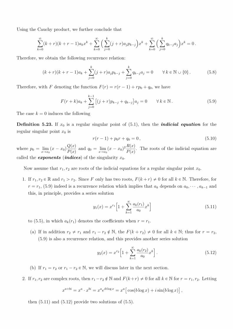
Using the Cauchy product, we further conclude that

8ÿ

k=0

(k + r)(k + r ´ 1)akxk +

8ÿ

k=0

( kÿ

j=0

(j + r)ajpk´j

)xk +

8ÿ

k=0

( kÿ

j=0

qk´jaj

)xk = 0 .

Therefore, we obtain the following recurrence relation:

(k + r)(k + r ´ 1)ak +kÿ

j=0

(j + r)ajpk´j +kÿ

j=0

qk´jaj = 0 @ k P N Y t0u . (5.8)

Therefore, with F denoting the function F (r) = r(r ´ 1) + rp0 + q0, we have

F (r + k)ak +k´1ÿ

j=0

[(j + r)pk´j + qk´j

]aj = 0 @ k P N . (5.9)

The case k = 0 induces the following

Definition 5.23. If x0 is a regular singular point of (5.1), then the indicial equation for theregular singular point x0 is

r(r ´ 1) + p0r + q0 = 0 , (5.10)

where p0 = limxÑx0

(x ´ x0)Q(x)

P (x)and q0 = lim

xÑx0

(x ´ x0)2R(x)

P (x). The roots of the indicial equation are

called the exponents (indices) of the singularity x0.

Now assume that r1, r2 are roots of the indicial equations for a regular singular point x0.

1. If r1, r2 P R and r1 ą r2. Since F only has two roots, F (k+ r) ‰ 0 for all k P N. Therefore, forr = r1, (5.9) indeed is a recurrence relation which implies that ak depends on a0, ¨ ¨ ¨ , ak´1 andthis, in principle, provides a series solution

y1(x) = xr1[1 +

8ÿ

k=1

ak(r1)

a0xk]

(5.11)

to (5.5), in which ak(r1) denotes the coefficients when r = r1.

(a) If in addition r2 ‰ r1 and r1 ´ r2 R N, the F (k + r2) ‰ 0 for all k P N; thus for r = r2,(5.9) is also a recurrence relation, and this provides another series solution

y2(x) = xr2[1 +

8ÿ

k=1

ak(r2)

a0xk]. (5.12)

(b) If r1 = r2 or r1 ´ r2 P N, we will discuss later in the next section.

2. If r1, r2 are complex roots, then r1 ´r2 R N and F (k+r) ‰ 0 for all k P N for r = r1, r2. Letting

xa+bi = xa ¨ xbi = xaeib logx = xa[

cos(b logx) + i sin(b logx)],

then (5.11) and (5.12) provide two solutions of (5.5).

Example 5.24. Solve the differential equation

2x2y 11 ´ xy 1 + (1 + x)y = 0 . (5.13)

We note that 0 is a regular singular point of the ODE above; thus we look for a series solution tothe ODE above of the form

y(x) = xr8ÿ

k=0

akxk .

Then r satisfies the indicial equation for 0

2r(r ´ 1) ´ r + 1 = 0

which implies that r = 1 or r = 1

2. Since

y 1(x) =8ÿ

k=0

(k + r)akxk+r´1 and y 11(x) =

8ÿ

k=0

(k + r)(k + r ´ 1)akxk+r´2 ,

we obtain that8ÿ

k=0

[2(k + r)(k + r ´ 1) ´ (k + r) + 1

]akx

k+r +8ÿ

k=0

akxk+r+1 = 0

or cancelling xr,8ÿ

k=0

[2(k + r)(k + r ´ 1) ´ (k + r) + 1

]akx

k +8ÿ

k=1

ak´1xk = 0 .

Therefore,ak = ´

ak´1

2(k + r)(k + r ´ 1) ´ (k + r) + 1@ k P N .

1. r = 1: ak = ´ak´1

k(2k + 1)for all k P N. Therefore,

ak = ´ak´1

k(2k + 1)=

ak´2

k(k ´ 1)(2k + 1)(2k ´ 1)= ´

ak´3

k(k ´ 1)(k ´ 2)(2k + 1)(2k ´ 1)(2k ´ 3)

=(´1)k

k!(2k + 1)(2k ´ 1) ¨ ¨ ¨ 1a0 =

(2k)(2k ´ 2)(2k ´ 4) ¨ ¨ ¨ 2(´1)k

k!(2k + 1)!a0 =

(´1)k2k

(2k + 1)!a0 .

This provides a series solution y1(x) =8ř

k=0

(´1)k2k

(2k + 1)!xk+1 whose radius of convergence is 8.

2. r = 1

2: ak = ´

ak´1

k(2k ´ 1)for all k P N. Therefore,

ak = ´ak´1

k(2k ´ 1)=

ak´2

k(k ´ 1)(2k ´ 1)(2k ´ 3)= ´

ak´3

k(k ´ 1)(k ´ 2)(2k ´ 1)(2k ´ 3)(2k ´ 5)

=(´1)k

k!(2k ´ 1)(2k ´ 3) ¨ ¨ ¨ 1a0 =

(´1)k(2k)(2k ´ 2) ¨ ¨ ¨ 2

k!(2k)!a0 =

(´1)k2k

(2k)!a0 .

This provides a series solution y2(x) =8ř

k=0

(´1)k2k

(2k)!xk+

12 whose radius of convergence is 8.

Therefore, the general solution to (5.13) in the series form is y = C1y1(x) + C2y2(x).

Example 5.25. Find a series solution about the regular singular point x = 0 of

(x+ 2)x2y 11(x) ´ xy 1(x) + (1 + x)y(x) = 0 , x ą 0 .

Let p(x) = ´1

x+ 2and q(x) =

1 + x

x+ 2. Then

p(x) = ´1

2

1

1 ´´x

2

= ´1

2

8ÿ

k=0

(´x)k

2k=

8ÿ

k=0

(´1)k+1xk

2k+1,

q(x) =x+ 1

x+ 2= 1 ´

1

2

1

1 ´´x

2

= 1 ´

8ÿ

k=0

(´1)kxk

2k+1=

1

2+

8ÿ

k=1

(´1)k+1xk

2k+1.

Therefore, (p0, q0) =(

´1

2,1

2

), and pk = qk =

(´1)k+1

2k+1for all k P N. The indicial equation for 0 is

r(r ´ 1) ´1

2r +

1

2= 0

which implies that r = 1 or r = 1

2.

1. r = 1: Suppose the series solution to the ODE is y = x8ř

k=0

akxk =

8ř

k=0

akxk+1. Then

(x+ 2)x28ÿ

k=0

(k + 1)kakxk´1 ´ x

8ÿ

k=0

(k + 1)akxk + (1 + x)

8ÿ

k=0

akxk+1 = 0

ñ

8ÿ

k=0

(k2 + k + 1)akxk+2 +

8ÿ

k=0

(2k2 + k)akxk+1 = 0

ñ

8ÿ

k=1

([(k ´ 1)2 + (k ´ 1) + 1]ak´1 + (2k2 + k)ak

)xk+1 = 0 .

Therefore, ak = ´k2 ´ k + 1

(2k + 1)kak´1 for all k P N. Note that

limkÑ8

ˇ

ˇ

ˇ

akak´1

ˇ

ˇ

ˇ= lim

kÑ8

ˇ

ˇ

ˇ

k2 ´ k + 1

k(2k + 1)

ˇ

ˇ

ˇ=

1

2;

thus the radius of convergence of the series solution y =8ř

k=0

akxk+1 is 2.

2. r = 1

2: Suppose the series solution to the ODE is y = x

12

8ř

k=0

akxk =

8ř

k=0

akxk+ 1

2 . Then

(x+ 2)8ÿ

k=0

(k +

1

2

)(k ´

1

2

)akx

k+ 12 ´

8ÿ

k=0

(k +

1

2

)akx

k+ 12 +

8ÿ

k=0

akxk+ 1

2 +8ÿ

k=0

akxk+ 3

2 = 0

ñ

8ÿ

k=0

(k2 +

3

4

)akx

k+ 32 +

8ÿ

k=0

(2k2 ´ k)akxk+ 1

2 = 0

ñ

8ÿ

k=0

(((k ´ 1)2 +

3

4

)ak´1 + (2k2 ´ k)ak

)xk+

12 = 0 .

Therefore, ak = ´(k ´ 1)2 + 3/4

k(2k ´ 1)ak´1 for all k P N. The radius of convergence of this series

solution is also 2.

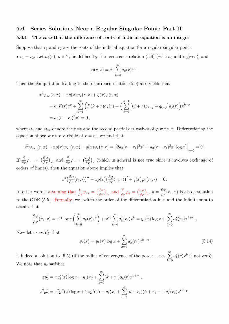
5.6 Series Solutions Near a Regular Singular Point: Part II5.6.1 The case that the difference of roots of indicial equation is an integer

Suppose that r1 and r2 are the roots of the indicial equation for a regular singular point.

‚ r1 = r2: Let ak(r), k P N, be defined by the recurrence relation (5.9) (with a0 and r given), and

φ(r, x) = xr8ÿ

k=0

ak(r)xk .

Then the computation leading to the recurrence relation (5.9) also yields that

x2φxx(r, x) + xp(x)φx(r, x) + q(x)φ(r, x)

= a0F (r)xr +

8ÿ

k=1

(F (k + r)ak(r) +

( k´1ÿ

j=0

[(j + r)pk´j + qk´j

]aj(r)

)xk+r

= a0(r ´ r1)2xr = 0 ,

where φx and φxx denote the first and the second partial derivatives of φ w.r.t.x. Differentiating theequation above w.r.t. r variable at r = r1, we find that

x2φxxr(r, x) + xp(x)φxr(r, x) + q(x)φr(r, x) =[2a0(r ´ r1)

2xr + a0(r ´ r1)2xr logx

]ˇˇ

ˇ

r=0= 0 .

If B

B rφxx =

(Bφ

B r

)xx

and B

B rφx =

(Bφ

B r

)x

(which in general is not true since it involves exchange of

orders of limits), then the equation above implies that

x2(Bφ

B r(r1, ¨)

) 11+ xp(x)

(Bφ

B r(r1, ¨)

) 1+ q(x)φr(r1, ¨) = 0 .

In other words, assuming that B

Brφxx =

(Bφ

B r

)xx

and B

B rφx =

(Bφ

B r

)x, y =

Bφ

B r(r1, x) is also a solution

to the ODE (5.5). Formally, we switch the order of the differentiation in r and the infinite sum toobtain that

Bφ

Br(r1, x) = xr1 logx

( 8ÿ

k=0

ak(r)xk)+ xr1

8ÿ

k=0

a 1k(r1)x

k = y1(x) logx+8ÿ

k=0

a 1k(r1)x

k+r1 .

Now let us verify that

y2(x) = y1(x) logx+8ÿ

k=0

a 1k(r1)x

k+r1 (5.14)

is indeed a solution to (5.5) (if the radius of convergence of the power series8ř

k=0

a 1k(r)x

k is not zero).

We note that y2 satisfies

xy 12 = xy 1

1(x) logx+ y1(x) +8ÿ

k=0

(k + r1)a1k(r)x

k+r1 ,

x2y 112 = x2y 11

1 (x) logx+ 2xy 1(x) ´ y1(x) +8ÿ

k=0

(k + r1)(k + r1 ´ 1)a 1k(r1)x

k+r1 .

Moreover, differentiating (5.8) w.r.t. r variable, we find that

[2(k + r1) ´ 1

]ak(r1) +

kÿ

j=0

pk´jaj(r1) +kÿ

j=0

[pk´j(j + r1) + qk´j

]a 1j(r1) = 0 @ k P N Y t0u .

Therefore, by the fact that y1 is a solution to (5.5), we have

x2y 112 + xp(x)y 1

2 + q(x)y2

= x2y 111 (x) logx+ 2xy 1

1(x) ´ y1(x) +8ÿ

k=0

(k + r1)(k + r ´ 1)a 1k(r1)x

k+r1

+ xp(x)y 11(x) logx+ p(x)y1(x) +

( 8ÿ

k=0

pkxk)( 8

ÿ

k=0

(k + r1)a1k(r1)x

k+r1)

+ q(x)y1(x) logx+( 8ÿ

k=0

qkxk)( 8

ÿ

k=0

a 1k(r1)x

k+r1)

=8ÿ

k=0

[2(k + r1) ´ 1

]ak(r1)x

k+r1 +8ÿ

k=0

( kÿ

j=0

pk´jaj(r1))xk+r1

+8ÿ

k=0

((k + r1)(k + r ´ 1)a 1

k(r1) +kÿ

j=0

[pk´j(j + r1) + qk´j

]a 1j(r1)

)xk+r1 = 0 ;

thus y2(x) is a solution to (5.5).

‚ r1 ´ r2 = N P N: using the recurrence relation (5.9) for r = r2, by the fact that F (r2 + N) =

F (r1) = 0 we cannot find aN(r2) so that aN+1(r2), aN+2(r2) and so on cannot be determined.

1. Suppose thatN´1ř

j=0

(j+ r)pN´j + qN´j is divisible by r´ r2 = r+N ´ r1. Since (5.9) implies that

(r ´ r2)(r +N ´ r2)aN(r) = ´

N´1ÿ

j=0

[(j + r)pN´j + qN´j

]aj(r) .

we can compute aN(r2) by

aN(r2) = limrÑr2

aN(r) = ´ limrÑr2

N´1ř

j=0(j + r)pN´j + qN´j

r ´ r2F (r +N)

r ´ r2

= ´1

NlimrÑr2

N´1ř

j=0

(j + r)pN´j + qN´j

r ´ r2;

thus the recurrence relation can be used to determine aN+1(r1), aN+2(r1) and so on. In such acase, another solution can be written by (5.12) as well.

2. In general (which includes the case thatN´1ř

j=0

(j + r)pN´j + qN´j is divisible by r ´ r2), we let

φ(r, x) = xr8ÿ

k=0

ak(r)xk ,

where ak(r) is given by the recurrence relation (5.9). Then

x2φxx(r, x) + xp(x)φx(r, x) + q(x)φ(r, x) = a0(r ´ r1)(r ´ r2)xr .

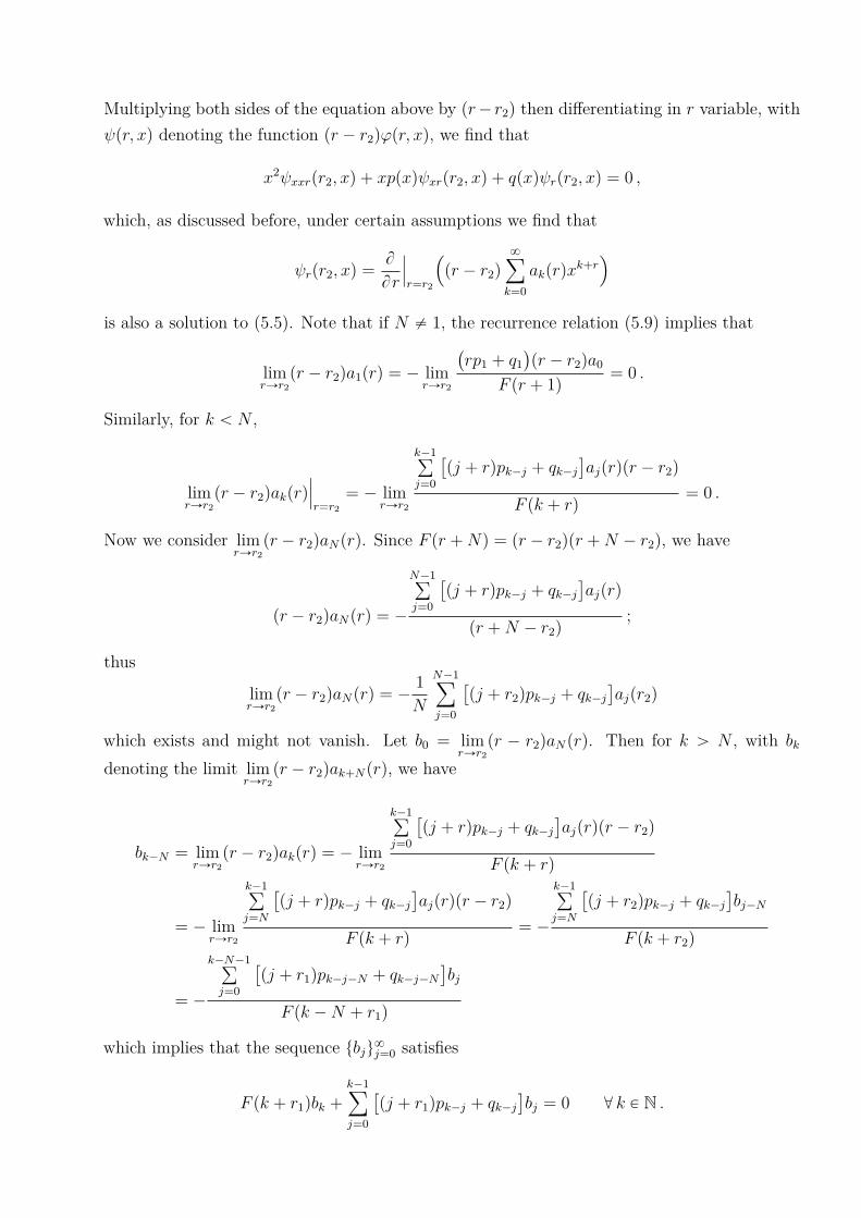
Multiplying both sides of the equation above by (r´ r2) then differentiating in r variable, withψ(r, x) denoting the function (r ´ r2)φ(r, x), we find that

x2ψxxr(r2, x) + xp(x)ψxr(r2, x) + q(x)ψr(r2, x) = 0 ,

which, as discussed before, under certain assumptions we find that

ψr(r2, x) =B

Br

ˇ

ˇ

ˇ

r=r2

((r ´ r2)

8ÿ

k=0

ak(r)xk+r

)is also a solution to (5.5). Note that if N ‰ 1, the recurrence relation (5.9) implies that

limrÑr2

(r ´ r2)a1(r) = ´ limrÑr2

(rp1 + q1

)(r ´ r2)a0

F (r + 1)= 0 .

Similarly, for k ă N ,

limrÑr2

(r ´ r2)ak(r)ˇ

ˇ

ˇ

r=r2= ´ lim

rÑr2

k´1ř

j=0

[(j + r)pk´j + qk´j

]aj(r)(r ´ r2)

F (k + r)= 0 .

Now we consider limrÑr2

(r ´ r2)aN(r). Since F (r +N) = (r ´ r2)(r +N ´ r2), we have

(r ´ r2)aN(r) = ´

N´1ř

j=0

[(j + r)pk´j + qk´j

]aj(r)

(r +N ´ r2);

thus

limrÑr2

(r ´ r2)aN(r) = ´1

N

N´1ÿ

j=0

[(j + r2)pk´j + qk´j

]aj(r2)

which exists and might not vanish. Let b0 = limrÑr2

(r ´ r2)aN(r). Then for k ą N , with bk

denoting the limit limrÑr2

(r ´ r2)ak+N(r), we have

bk´N = limrÑr2

(r ´ r2)ak(r) = ´ limrÑr2

k´1ř

j=0

[(j + r)pk´j + qk´j

]aj(r)(r ´ r2)

F (k + r)

= ´ limrÑr2

k´1ř

j=N

[(j + r)pk´j + qk´j

]aj(r)(r ´ r2)

F (k + r)= ´

k´1ř

j=N

[(j + r2)pk´j + qk´j

]bj´N

F (k + r2)

= ´

k´N´1ř

j=0

[(j + r1)pk´j´N + qk´j´N

]bj

F (k ´ N + r1)

which implies that the sequence tbju8j=0 satisfies

F (k + r1)bk +k´1ÿ

j=0

[(j + r1)pk´j + qk´j

]bj = 0 @ k P N .

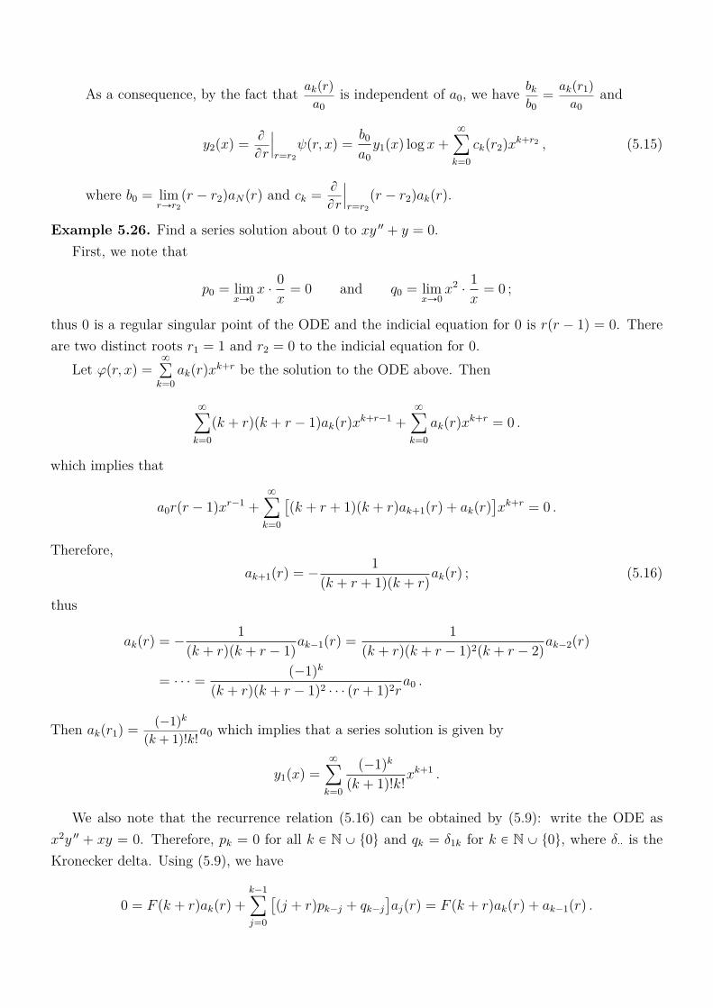
As a consequence, by the fact that ak(r)

a0is independent of a0, we have bk

b0=

ak(r1)

a0and

y2(x) =B

Br

ˇ

ˇ

ˇ

r=r2ψ(r, x) =

b0a0y1(x) logx+

8ÿ

k=0

ck(r2)xk+r2 , (5.15)

where b0 = limrÑr2

(r ´ r2)aN(r) and ck =B

Br

ˇ

ˇ

ˇ

r=r2(r ´ r2)ak(r).

Example 5.26. Find a series solution about 0 to xy 11 + y = 0.First, we note that

p0 = limxÑ0

x ¨0

x= 0 and q0 = lim

xÑ0x2 ¨

1

x= 0 ;

thus 0 is a regular singular point of the ODE and the indicial equation for 0 is r(r ´ 1) = 0. Thereare two distinct roots r1 = 1 and r2 = 0 to the indicial equation for 0.

Let φ(r, x) =8ř

k=0

ak(r)xk+r be the solution to the ODE above. Then

8ÿ

k=0

(k + r)(k + r ´ 1)ak(r)xk+r´1 +

8ÿ

k=0

ak(r)xk+r = 0 .

which implies that

a0r(r ´ 1)xr´1 +8ÿ

k=0

[(k + r + 1)(k + r)ak+1(r) + ak(r)

]xk+r = 0 .

Therefore,ak+1(r) = ´

1

(k + r + 1)(k + r)ak(r) ; (5.16)

thus

ak(r) = ´1

(k + r)(k + r ´ 1)ak´1(r) =

1

(k + r)(k + r ´ 1)2(k + r ´ 2)ak´2(r)

= ¨ ¨ ¨ =(´1)k

(k + r)(k + r ´ 1)2 ¨ ¨ ¨ (r + 1)2ra0 .

Then ak(r1) =(´1)k

(k + 1)!k!a0 which implies that a series solution is given by

y1(x) =8ÿ

k=0

(´1)k

(k + 1)!k!xk+1 .

We also note that the recurrence relation (5.16) can be obtained by (5.9): write the ODE asx2y 11 + xy = 0. Therefore, pk = 0 for all k P N Y t0u and qk = δ1k for k P N Y t0u, where 䨨 is theKronecker delta. Using (5.9), we have

0 = F (k + r)ak(r) +k´1ÿ

j=0

[(j + r)pk´j + qk´j

]aj(r) = F (k + r)ak(r) + ak´1(r) .

We summarize the discussions above into the following

Theorem 5.27. Let x0 = 0 be a regular singular point of the differential equation (5.5), and r1 andr2 be the roots of the indicial equation (5.10) with r1 ě r2 if r1, r2 P R. Then there exists a seriessolution given by (5.11).

1. If r1 ´ r2 R N Y t0u, then another solution is given by (5.12).

2. If r1 = r2, then another solution is given by (5.14).

3. If r1 ´ r2 = N P N, then another solution is given by (5.15).

In all three cases, the two solutions y1 and y2 form a fundamental set of solutions of the givendifferential equation.

5.6.2 The radius of convergence of series solutions

The radius of convergence of the series solution (5.7) cannot be guaranteed by Theorem 5.19; however,we have the following

Theorem 5.28 (Frobenius). If x0 is a regular singular point of ODE (5.1), then there exists at leastone series solution of the form

y(x) = (x ´ x0)r

8ÿ

k=0

ak(x ´ x0)k ,

where r is the largest root of the associated indicial equation. Moreover, the series solution convergesfor all x P 0 ă x ´ x0 ă R, where R is the distance from x0 to the nearest other singular point (realor complex) of (5.1).

5.7 Bessel’s Equation

We consider three special cases of Bessel’s equation

x2y 11 + xy 1 + (x2 ´ ν2)y = 0 , (5.17)

where ν is a constant. It is easy to see that x = 0 is a regular singular point of (5.17) since

limxÑ0

x ¨x

x2= 1 = p0 and lim

xÑ0x2 ¨

x2 ´ ν2

x2= ´ν2 = q0 .

Therefore, the indicial equation for the regular singular point x = 0 is

r(r ´ 1) + r ´ ν2 = 0

which implies that r = ˘ν. The ODE (5.17) is called Bessel’s equation of order ν.To find series solution to (5.17), we first note that in the case of Bessel’s equation of order ν,

F (r) = r2 ´ ν2, p(x) = 1 (which implies that p0 = 1 while pk = 0 for all k P N) and q(x) = x2 ´ ν2

(which implies that q0 = ´ν2 and q2 = 1 and qk = 0 otherwise). Therefore, the recurrence relation(5.9) implies that [

(k + r)2 ´ ν2]ak(r) +

k´1ÿ

j=0

qk´jaj(r) = 0 @ k P N .

This implies that [(1 + r)2 ´ ν2

]a1(r) = 0 (5.18a)[

(k + r)2 ´ ν2]ak(r) + ak´2(r) = 0 @ k ě 2 (5.18b)

5.7.1 Bessel’s Equation of Order Zero

Consider the case ν = 0. Then the roots of the indicial equation are identical: r1 = r2 = 0. Using(5.18a), a1(r) ” 0 (in a small neighborhood of 0) and (5.18b) implies that

ak(r) = ´1

(k + r)2ak´2(r) @ k ě 2 ; (5.19)

thus a3(r) = a5(r) = ¨ ¨ ¨ = a2m+1(r) = ¨ ¨ ¨ = 0 for all m P N. Note that a2m´1(r) = 0 for all m P Nalso implies that a 1

2m´1(r) = 0 for all m P N.On the other hand, recurrence relation (5.19) also implies that

a2m(r) = ´1

(2m+ r)2a2m´2(r) =

1

(2m+ r)2(2m+ r ´ 2)2a2m´4(r)

= ¨ ¨ ¨ =(´1)m´1

(2m+ r)2(2m+ r ´ 2)2 ¨ ¨ ¨ (4 + r)2a2(r)

=(´1)m

(2m+ r)2(2m+ r ´ 2)2 ¨ ¨ ¨ (4 + r)2(2 + r)2a0 ;

thus a2m(0) =(´1)m

22m(m!)2a0 and rearranging terms, we obtain that

log (´1)ma2m(r)

a0= ´2

[log(2m+ r) + log(2m+ r ´ 2) + ¨ ¨ ¨ + log(4 + r) + log(2 + r)

].

Differentiating both sides above in r,

a 12m(r)

a2m(r)= ´2

[ 1

2m+ r+

1

2m+ r ´ 2+ ¨ ¨ ¨ +

1

4 + r+

1

2 + r

],

and evaluating the equation above at r = 0 we conclude that

a 12m(0) = ´Hma2m(0) =

(´1)m+1Hm

22m(m!)2a0 ,

where Hm =mř

k=1

1

k. As a consequence, the first series solution is given by

y1(x) =8ÿ

k=0

a2k(0)x2k = a0

[1 +

8ÿ

k=1

(´1)kx2k

22k(k!)2

],

and the second solution is given by

y2(x) = a0

[J0(x) logx+

8ÿ

k=1

(´1)kHkx2k

22k(k!)2

],

where J0 = a´10 y1 is called the Bessel function of the first kind of order zero. We note that

y1 and y2 can be defined for all x ą 0 since the radius of convergence of the series involved in y1 andy2 are infinite.

Any linear combinations of y1 and y2 is also a solution to Bessel’s equation (5.17) of order zero.Consider the Bessel function of the second kind of order zero

Y0(x) =2

π

[ 1

a0y2(x) + (γ ´ log 2)J0(x)

], (5.20)

where γ = limkÑ8

(Hk ´ log k) « 0.5772 is called the Euler-Máscheroni constant. Substituting fory2 in (5.20), we obtain

Y0(x) =2

π

[(γ + log x

2

)J0(x) +

8ÿ

k=1

(´1)k+1Hk

22k(k!)2x2k

], x ą 0 . (5.21)

A general solution to Bessel’s equation (5.17) of order zero then can be written as

y(x) = C1J0(x) + C2Y0(x) .

‚ Properties of J0 and Y0:

J0(x) «

c

2

πxcos

(x ´

π

4

)as x Ñ 8 ,

Y0(x) «

c

2

πxsin

(x ´

π

4

)as x Ñ 8 .

5.7.2 Bessel’s Equation of Order One-Half

Now suppose that ν =1

2(thus r1 =

1

2and r2 = ´

1

2). To obtain solutions to Bessel’s equation

(5.17) of order one-half, we need to compute the coefficients ak(r) for all k P N (given a0), and

b0 = limrÑ´ 1

2

(r ´ r2)a1(r) as well as ck =B

Br

ˇ

ˇ

ˇ

r=r2(r ´ r2)ak(r).

Using (5.18b), we find that

ak(r) =´1

(k + r)2 ´ 14

ak´2(r) =´1

(k + r + 12)(k + r ´ 1

2)ak´2(r) @ k ě 2 ,

while if r « r1 =1

2, (5.18a) implies that a1(r) = 0 which further implies that a3(r) = a5(r) = ¨ ¨ ¨ =

a2m´1(r) = ¨ ¨ ¨ = 0 for all m P N if r «1

2. In particular, we have

a2m(1

2) =

(´1)ma0(2m+ 1)!

and a2m´1(1

2) = 0 @m P N ;

thus a series solution of (5.17) is

y1(x) = a0x12

8ÿ

k=0

(´1)kx2k

(2k + 1)!= a0x

´ 12

8ÿ

k=0

(´1)kx2k+1

(2k + 1)!= a0

sin x?x.

The Bessel function of the first kind of order one-half is defined by (letting a0 =b

2

πin

the expression of y1 above)

J 12(x) =

c

2

π

sin x?x

=

c

2

πxsinx .

Now we compute the limit of (r ´ r2)a1(r) as r approaches r2. Since (5.18a) implies that (r +3

2)(r +

1

2)a1(r) = 0, we have (r ´ r2)a1(r) = 0 for all r « r2 = ´

1

2. Therefore,

b0 = limrÑr2

(r ´ r2)a1(r) = 0

which implies that there will be no logarithmic term in the second solution y2 given by (5.12).

Now we compute B

Br

ˇ

ˇ

ˇ

r=r2(r ´ r2)ak(r). Since

a2m(r) =´1

(2m+ r + 12)(2m+ r ´ 1

2)a2m´2(r) = ¨ ¨ ¨

=(´1)m

(2m+ r + 12)(2m+ r ´ 1

2) ¨ ¨ ¨ (2 + r + 1

2)(2 + r ´ 1

2)a0

=(´1)m

(2m+ r + 12)(2m+ r ´ 1

2) ¨ ¨ ¨ (r + 5

2)(r + 3

2)a0

which implies that |a 12m(r2)| ă 8. Therefore,

c2m(r2) =B

Br

ˇ

ˇ

ˇ

r=r2(r ´ r2)a2m(r) = a2m(r2) =

(´1)m

(2m)!a0 .

On the other hand, using (5.18a) again, we find that a1(r2) is not necessary zero; thus we let a1be a free constant and use (5.18b) to obtain that

a2m+1(r) =(´1)m

(2m+ 1 + r + 12)(2m+ 1 + r ´ 1

2) ¨ ¨ ¨ (3 + r + 1

2)(3 + r ´ 1

2)a1 .

Since |a 12m+1(r2)| ă 8, we find that

c2m+1(r2) =B

Br

ˇ

ˇ

ˇ

r=r2(r ´ r2)a2m+1(r) = a2m(r2) =

(´1)m

(2m+ 1)!a1 .

Therefore,

y2(x) =8ÿ

k=0

ck(r2)xk+r2 = x´ 1

2

[a0

8ÿ

k=1

(´1)m

(2k)!x2k + a1

8ÿ

k=1

(´1)k

(2k ´ 1)!x2k´1

]= a0

cosx?x

+ a1sinx?x.

This produces the Bessel function of the second kind of order one-half

J´ 12(x) =

c

2

πxcosx ,

and the general solution of Bessel’s equation of order one-half can be written as y = C1J 12(x) +

C2J´ 12(x).

5.7.3 Bessel’s Equation of Order One

Now we consider the case that ν = 1 (thus r1 = 1 and r2 = ´1). Again, we need to compute

ak(r1)(8

k=1, limrÑr2

(r ´ r2)a2(r) and ck(r2) =B

Br

ˇ

ˇ

ˇ

r=r2(r ´ r2)ak(r).

Note that (5.18a) implies that a1(r1) = 0 (which implies that a2m´1(r1) = 0 for all m P N).Moreover,

a2m(r1) =´1

(2m+ 2)2ma2m´2(r) =

1

(2m+ 2)(2m)2(2m ´ 2)a2m´4(r)

= ¨ ¨ ¨ =(´1)m

(2m+ 2)(2m)2(2m ´ 4)2 ¨ ¨ ¨ 42 ¨ 2a0 =

(´1)m

22m(m+ 1)!m!a0 ;

thusy1(x) = a0x

8ÿ

k=0

(´1)k

22k(k + 1)!k!x2k .

Now we focus on finding b0 and

ck(r2)(8

k=0. Note that by (5.18a),

F (2 + r)a2(r) = ´a0 ;

thus (r + 1)a2(r) = ´1

2(r + 3)which implies that b0 = lim

rÑr2(r ´ r2)a2(r) = ´

a02

.

To compute

ck(r2)(8

k=0, we first note that (5.18a) implies that a1(r) ” 0; thus we use (5.18b) to

conclude that a2m´1(r) = 0 for all m P N and r « r2. This implies that c2m´1(r2) = 0 for all m P N.On the other hand, for m P N and r « r2,

a2m(r) =(´1)m

(2m+ r + 1)(2m+ r ´ 1)2 ¨ ¨ ¨ (r + 3)2(r + 1)a0 ;

thus(r ´ r2)a2m(r) =

(´1)m

(2m+ r + 1)(2m+ r ´ 1)2 ¨ ¨ ¨ (r + 3)2a0 .

Therefore, using the formula d

drf(r) = f(r)

d

drlog f(r) if f(r) ą 0, we find that

c2m(r2) =(´1)m+1a0

(2m)(2m ´ 2)2 ¨ ¨ ¨ 22

[ 1

2m+ r + 1+

2

2m+ r ´ 1+ ¨ ¨ ¨ +

2

r + 3

]ˇˇ

ˇ

r=r2

=(´1)m+1a0

22m´1m!(m ´ 1)!

[ 1

2m+

2

2m ´ 2+ ¨ ¨ ¨ +

2

2

]=

(´1)m+1a022mm!(m ´ 1)!

[ 1

m+

2

m ´ 1+ ¨ ¨ ¨ +

2

1

]=

(´1)m+1(Hm +Hm´1

)22mm!(m ´ 1)!

a0 .

Moreover, c0(r2) =B

Br

ˇ

ˇ

ˇ

r=r2(r ´ r2)a0 = a0. Then the second solution to Bessel’s equation of order

one is

y2(x) =b0a0y1(x) logx+

8ÿ

k=0

ck(r2)xk+r2 = ´J1(x) logx+ x´1

[a0 +

8ÿ

k=1

c2k(r2)x2k]

= ´1

2y1(x) logx+ a0

x

[1 ´

8ÿ

k=1

(´1)k(Hk +Hk´1)

22kk!(k ´ 1)!x2k

].

This produces the Bessel function of the first kind of order one:

J1(x) ”1

2y1(x) =

x

2

8ÿ

k=0

(´1)k

22k(k + 1)!k!x2k

and the Bessel function of the second kind of order one:

Y1(x) ”2

π

[´ y2(x) + (γ ´ log 2)J1(x)

],

where γ is again the Euler-Máscheroni constant. The general solution to Bessel’s equation of orderone then can be written as

y = C1J1(x) + C2Y1(x) .

6 System of First Order Linear Equations

6.1 Introduction

There are several reasons that we should consider system of first order ODEs, and here we providetwo of them.

1. In real life, a lot of phenomena can be modelled by system of first order ODE. For example,the LotkaVolterra equation or the predator-prey equation:

p1 = γp ´ αpq ,

q1 = βq + δpq .

in Example 1.10 can be used to described a predator-prey system. Let x ” (x1, x2) = (p, q)T

and F(t,x) = (γx1 ´ αx1x2, βx2 + δx1x2)T. Then the Lotka-Volterra equation can also be

written asx 1(t) = F

(t,x(t)

). (6.1)

2. Suppose that we are considering a scalar n-th order ODE

y(n)(t) = f(t, y(t), y 1(t), ¨ ¨ ¨ , y(n´1)(t)

).

Let x1(t) = y(t), x2(t) = y 1(t), ¨ ¨ ¨ , xn(t) = y(n´1)(t). Then (x1, ¨ ¨ ¨ , xn) satisfies

x 11(t) = x2(t) , (6.2a)

x 12(t) = x3(t) , (6.2b)... =

... (6.2c)

x 1n(t) = f

(t, x1(t), x2(t), ¨ ¨ ¨ , xn(t)

). (6.2d)

Let x = (x1, ¨ ¨ ¨ , xn)T be an n-vector, and F(t,x) =

(x2, x3, ¨ ¨ ¨ , xn, f(t, x1, x2, ¨ ¨ ¨ , xn)

)T be avector-valued function. Then (6.2) can also be written as (6.1).

Definition 6.1. The system of ODE (6.1) is said to be linear if F is of the form

F(t,x) = P(t)x + g(t)

for some matrix-valued function P =[pij(t)

]nˆn

. (6.1) is said to be homogeneous if g(t) = 0.

Example 6.2. Consider the second order ODE

y 11 ´ y 1 ´ 2y = sin t . (6.3)

Let x1(t) = y(t) and x2(t) = y 1(t). Then x = (x1, x2)T satisfies

x 1(t) =

[0 12 1

]x(t) +

[0

sin t

]. (6.4)

Therefore, the second order linear ODE (6.3) corresponds to a system of first order linear ODE (6.4).Review: to solve (6.3), we use the method of variation of parameters and assume that the solutionto (6.3) can be written as

y(t) = u1(t)e2t + u2(t)e

´t ,

where te2t, e´tu is a fundamental set of (6.3). By the additional assumption u 11(t)e

2t + u 12e

´t = 0, wefind that [

e2t e´t

2e2t ´e´t

] [u 11

u 12

]=

[0

sin t

].

Therefore, with W (t) denoting the Wronskian of te2t, e´tu, we have

u 11(t) =

1

W (t)det

([0 e´t

sin t ´e´t

])=

´e´t sin t´3et

=1

3e´2t sin t

andu 12(t) =

1

W (t)det

([e2t 02e2t sin t

])=e2t sin t´3et

= ´1

3et sin t

which further implies that a particular solution is

y(t) = ´2e´2t sin t+ e´2t cos t

15e2t +

et cos t ´ et sin t6

e´t

= ´2 sin t+ cos t

15+

cos t ´ sin t6

=cos t ´ 3 sin t

10.

This particular solution provides a particular solution to (6.4):

x(t) =[y(t)y 1(t)

]=

cos t ´ 3 sin t

10

´sin t+ 3 cos t

10

.

Example 6.3. The ODE

x 1 =

[1 14 1

]x (6.5)

is a system of first order linear homogeneous ODE. Suppose the initial condition is given by x(0) =(x10, x20)

T.

1. Let x = (x1, x2)T. Then

x 11(t) = x1(t) + x2(t) , (6.6a)

x 12(t) = 4x1(t) + x2(t) . (6.6b)

Note that (6.6a) implies x2 = x 11 ´ x1; thus replacing x2 in (6.6) by x2 = x 1

1 ´ x1 we find that

x 111 ´ x1

1 = 4x1 + x 11 ´ x1 or x 11

1 ´ 2x 11 ´ 3x1 = 0 .

Therefore, x1(t) = C1e3t + C2e

´t and this further implies that x2(t) = 2C1e3t ´ 2C2e

´t; thusthe solution to (6.5) can be expressed as

x(t) =[x1(t)x2(t)

]= C1

[12

]e3t + C2

[1

´2

]e´t .

2. Let xh(k) « x(kh) = (x1(kh), x2(kh))T be the approximated value of x at the k-th step. Since

x((k + 1)h) « x(kh) + h

[1 14 1

]xh(k) ,

we consider the (explicit) Euler scheme

xh(k + 1) = xh(k) + h

[1 14 1

]xh(k) =

(Id + h

[1 14 1

])k[x10x20

],

and we expect that for t ą 0 and k = t/h, then xh(k) Ñ x(t) as h Ñ 0.

To compute the k-th power of the matrix Id + h

[1 14 1

], we diagonize the matrix and obtain

thatId + h

[1 14 1

]=

[1 + h h4h 1 + h

]=

[1 1

´2 2

] [1 ´ h 00 1 + 3h

] [1 1

´2 2

]´1

;

thus (Id + h

[1 14 1

])k

=

[1 1

´2 2

] [(1 ´ h)k 0

0 (1 + 3h)k

] [1 1

´2 2

]´1

.

As a consequence, using the limit (1 ´ h)th Ñ e´t and (1 + 3h)

th Ñ e3t as t Ñ 0, we find that

x(t) = limhÑ0

xh

( t

h

)=

[1 1

´2 2

] [e´t 00 e3t

] [1 1

´2 2

]´1 [x10x20

]=

1

4

[1 1

´2 2

] [e´t 00 e3t

] [2 ´12 1

] [x10x20

]=

1

4

[2e´t + 2e3t ´e´t + e3t

´4e´t + 4e3t 2e´t + 2e3t

] [x10x20

]=

1

4

[2x10 + x204x10 + 2x20

]e3t +

1

4

[2x10 ´ x20

´4x10 + 2x20

]e´t .

Choose x0 = (1, 2)T and x0 = (1,´2)T, we find that

x1(t) =

[12

]e3t and x2(t) =

[1

´2

]e´t

are both solution to (6.5).

Remark 6.4. For a, b, c, d P R being given constants, suppose that x1 and x2 satisfy the system offirst order linear ODE

x 11 = ax1 + bx2 , (6.7a)

x 12 = cx1 + dx2 . (6.7b)

Using (6.7a), we have bx2 = x 11 ´ ax2; thus (6.7b) implies that x1 satisfies

x 111 ´ (a+ d)x 1

1 + (ad ´ bc)x1 = 0 .

We note that the characteristic equation for the ODE above is exactly the characteristic equation of

the matrix[a bc d

].

Moreover, suppose that λ1 ‰ λ2 are distinct zeros of the characteristic equation, then

x1(t) = C1eλ1t + C2e

λ2t .

Similarly, x2(t) = C3eλ1t + C4e

λ2t for some C3, C4 satisfying

λ1C1eλ1t + λ2C2e

λ2t = (aC1 + bC3)eλ1t + (aC2 + bC4)e

λ2t ,

λ1C3eλ1t + λ2C2e

λ2t = (cC1 + dC3)eλ1t + (cC2 + dC4)e

λ2t .

Since teλ1t, eλ2tu are linearly independent, we must have that C1, C2, C3, C4 satisfy[a bc d

] [C1

C3

]= λ1

[C1

C3

]and

[a bc d

] [C2

C4

]= λ2

[C2

C4

].

In other words, (C1, C3)T and (C2, C4)

T are the eigenvectors of[a bc d

]associated with eigenvalues

λ1 and λ2, respectively. Therefore,

x(t) =[C1e

λ1t + C2eλ2t

C3eλ1t + C4e

λ2t

]=

[C1

C3

]eλ1t +

[C2

C4

]eλ2t = u1e

λ1t + u2eλ2t ,

where u1 = (C1, C3)T and u2 = (C2, C4)

T.

6.2 Basic Theory of Systems of First Order Equations

Similar to Theorem 2.10, we have the following

Theorem 6.5. Let x0 = (x10, x20, ¨ ¨ ¨ , xn0) be a point in Rn, V Ď Rn be an open set containing x0,and F : (α, β) ˆ V Ñ Rn be a vector-valued function of t and x such that F = (F1, ¨ ¨ ¨ , Fn) and thepartial derivative BFi

Bxjis continuous in (α, β) ˆ V for all i, j P t1, 2, ¨ ¨ ¨ , nu. Then in some interval

t P (t0 ´ h, t0 + h) Ď (α, β), there exists a unique solution x = φ(t) to the initial value problem

x 1 = F(t,x) x(t0) = x0 . (6.8)

Moreover, if (6.8) is linear and V = Rn, then the solution exists throughout the interval (α, β).

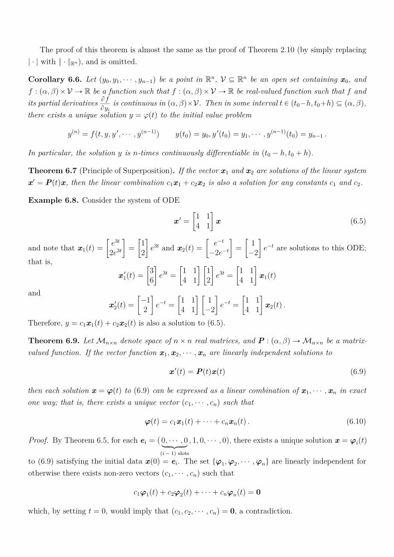
The proof of this theorem is almost the same as the proof of Theorem 2.10 (by simply replacing| ¨ | with ¨ Rn), and is omitted.

Corollary 6.6. Let (y0, y1, ¨ ¨ ¨ , yn´1) be a point in Rn, V Ď Rn be an open set containing x0, andf : (α, β)ˆV Ñ R be a function such that f : (α, β)ˆV Ñ R be real-valued function such that f andits partial derivatives Bf

Byiis continuous in (α, β)ˆV. Then in some interval t P (t0´h, t0+h) Ď (α, β),

there exists a unique solution y = φ(t) to the initial value problem

y(n) = f(t, y, y 1, ¨ ¨ ¨ , y(n´1)) y(t0) = y0, y1(t0) = y1, ¨ ¨ ¨ , y(n´1)(t0) = yn´1 .

In particular, the solution y is n-times continuously differentiable in (t0 ´ h, t0 + h).

Theorem 6.7 (Principle of Superposition). If the vector x1 and x2 are solutions of the linear systemx 1 = P(t)x, then the linear combination c1x1 + c2x2 is also a solution for any constants c1 and c2.

Example 6.8. Consider the system of ODE

x 1 =

[1 14 1

]x (6.5)

and note that x1(t) =

[e3t

2e3t

]=

[12

]e3t and x2(t) =

[e´t

´2e´t

]=

[1

´2

]e´t are solutions to this ODE;

that is,

x 11(t) =

[36

]e3t =

[1 14 1

] [12

]e3t =

[1 14 1

]x1(t)

andx 12(t) =

[´12

]e´t =

[1 14 1

] [1

´2

]e´t =

[1 14 1

]x2(t) .

Therefore, y = c1x1(t) + c2x2(t) is also a solution to (6.5).

Theorem 6.9. Let Mnˆn denote space of nˆ n real matrices, and P : (α, β) Ñ Mnˆn be a matrix-valued function. If the vector function x1,x2, ¨ ¨ ¨ ,xn are linearly independent solutions to

x 1(t) = P(t)x(t) (6.9)

then each solution x = φ(t) to (6.9) can be expressed as a linear combination of x1, ¨ ¨ ¨ ,xn in exactone way; that is, there exists a unique vector (c1, ¨ ¨ ¨ , cn) such that

φ(t) = c1x1(t) + ¨ ¨ ¨ + cnxn(t) . (6.10)

Proof. By Theorem 6.5, for each ei = (0, ¨ ¨ ¨ , 0looomooon

(i ´ 1) slots

, 1, 0, ¨ ¨ ¨ , 0), there exists a unique solution x = φi(t)

to (6.9) satisfying the initial data x(0) = ei. The set tφ1,φ2, ¨ ¨ ¨ ,φnu are linearly independent forotherwise there exists non-zero vectors (c1, ¨ ¨ ¨ , cn) such that

c1φ1(t) + c2φ2(t) + ¨ ¨ ¨ + cnφn(t) = 0

which, by setting t = 0, would imply that (c1, c2, ¨ ¨ ¨ , cn) = 0, a contradiction.

We note that tφ1, ¨ ¨ ¨ ,φnu is a fundamental set since every solution x(t) to (6.9) can be uniquelyexpressed by

x(t) = x1(0)φ1(t) + x2(0)φ2(t) + ¨ ¨ ¨ + xn(0)φn(t) . (6.11)

In fact, x(t) and x1(0)φ1(t) + ¨ ¨ ¨ + xn(0)φn(t) are both solutions to (6.9) satisfying the initial data

x(0) =(x1(0), ¨ ¨ ¨ , xn(0)

)T;

thus by uniqueness of the solution, (6.11) holds.Now, since x1, ¨ ¨ ¨ ,xn are solution to (6.9), we find that

span(x1, ¨ ¨ ¨ ,xn) Ď span(φ1, ¨ ¨ ¨ ,φn) .

Since tx1, ¨ ¨ ¨ ,xnu are linearly independent, dim(span(x1, ¨ ¨ ¨ ,xn)

)= n; thus by the fact that

dim(span(φ1, ¨ ¨ ¨ ,φn)

)= n, we must have

span(x1, ¨ ¨ ¨ ,xn) = span(φ1, ¨ ¨ ¨ ,φn) .

Therefore, every solution x = φ(t) of (6.9) can be (uniquely) expressed by (6.10). ˝

Definition 6.10. Let P(t) P Mnˆn, and x1, ¨ ¨ ¨ ,xn be linearly independent solutions to (6.9). Thentx1, ¨ ¨ ¨ ,xnu is called a fundamental set of (6.9), the matrix Ψ(t) =

[[x1(t)]

... [x2(t)]... ¨ ¨ ¨

... [xn(t)]]

is called the fundamental matrix of (6.9), and φ(t) = c1x1(t)+ ¨ ¨ ¨+cnxn(t) is called the generalsolution of (6.9).

Theorem 6.11. If φ1,φ2, ¨ ¨ ¨ ,φn are solutions to (6.9), then

det([[φ1

] ...[φ2

] ... ¨ ¨ ¨...[φn

]])

is either identically zero or else never vanishes.

Recall Theorem 4.3 that for a collection of solutions tφ1, ¨ ¨ ¨ , φnu to a n-th order ODE

y(n) + pn´1(t)y(n´1) + ¨ ¨ ¨ + p1y

1 + p0y = 0 ,

the derivative of Wronskian W (t) =

ˇ

ˇ

ˇ

ˇ

ˇ

ˇ

ˇ

ˇ

ˇ

φ1 φ2 ¨ ¨ ¨ φn

φ 11 φ 1

2 ¨ ¨ ¨ φ 1n

... . . . ...φ(n´1)1 φ

(n´1)2 ¨ ¨ ¨ φ

(n´1)n

ˇ

ˇ

ˇ

ˇ

ˇ

ˇ

ˇ

ˇ

ˇ

satisfies

d

dtW (t) = ´pn´1(t)W (t)

which can be used to show that W (t) is identically zero or else never vanishes. We use the same ideaand try to find the derivative of the determinant W(t) ” det(

[[φ1

] ...[φ2

] ... ¨ ¨ ¨...[φn

]]). In view of

Remark 6.4, we expect that we can derive

d

dtW(t) = tr(P)W(t) .

Proof. Let W(t) ” det([[φ1

] ...[φ2

] ... ¨ ¨ ¨...[φn

]]), P = [pij]nˆn, and the i-th component of φj be φ(i)

j ;that is, [

φj

]=

[φ(1)j , ¨ ¨ ¨ , φ

(n)j

]T.

Since φ(i)1j =

nř

k=1

pikφ(k)j , using the properties of the determinants we find that

ˇ

ˇ

ˇ

ˇ

ˇ

ˇ

ˇ

ˇ

ˇ

ˇ

ˇ

ˇ

ˇ

ˇ

ˇ

ˇ

ˇ

φ(1)1 φ

(1)2 ¨ ¨ ¨ ¨ ¨ ¨ φ

(1)n

... ... ...φ(j´1)1 φ

(j´1)2 ¨ ¨ ¨ ¨ ¨ ¨ φ

(j´1)n

φ(j)11 φ

(j)12 ¨ ¨ ¨ ¨ ¨ ¨ φ

(j)1n

φ(j+1)1 φ

(j+1)2 ¨ ¨ ¨ ¨ ¨ ¨ φ

(j+1)n

... ... ...φ(n)1 φ

(n)2 ¨ ¨ ¨ ¨ ¨ ¨ φ

(n)n

ˇ

ˇ

ˇ

ˇ

ˇ

ˇ

ˇ

ˇ

ˇ

ˇ

ˇ

ˇ

ˇ

ˇ

ˇ

ˇ

ˇ

=

ˇ

ˇ

ˇ

ˇ

ˇ

ˇ

ˇ

ˇ

ˇ

ˇ

ˇ

ˇ

ˇ

ˇ

ˇ

ˇ

ˇ

ˇ

φ(1)1 φ

(1)2 ¨ ¨ ¨ ¨ ¨ ¨ φ

(1)n

... ... ...φ(j´1)1 φ

(j´1)2 ¨ ¨ ¨ ¨ ¨ ¨ φ

(j´1)n

nř

k=1

pjkφ(k)1

nř

k=1

pjkφ(k)2 ¨ ¨ ¨ ¨ ¨ ¨

nř

k=1

pjkφ(k)n

φ(j+1)1 φ

(j+1)2 ¨ ¨ ¨ ¨ ¨ ¨ φ

(j+1)n

... ... ...φ(n)1 φ

(n)2 ¨ ¨ ¨ ¨ ¨ ¨ φ

(n)n

ˇ

ˇ

ˇ

ˇ

ˇ

ˇ

ˇ

ˇ

ˇ

ˇ

ˇ

ˇ

ˇ

ˇ

ˇ

ˇ

ˇ

ˇ

“row operations”=

ˇ

ˇ

ˇ

ˇ

ˇ

ˇ

ˇ

ˇ

ˇ

ˇ

ˇ

ˇ

ˇ

ˇ

ˇ

ˇ

ˇ

φ(1)1 φ

(1)2 ¨ ¨ ¨ ¨ ¨ ¨ φ

(1)n

... ... ...φ(j´1)1 φ

(j´1)2 ¨ ¨ ¨ ¨ ¨ ¨ φ

(j´1)n

pjjφ(j)1 pjjφ

(j)2 ¨ ¨ ¨ ¨ ¨ ¨ pjjφ

(j)n

φ(j+1)1 φ

(j+1)2 ¨ ¨ ¨ ¨ ¨ ¨ φ

(j+1)n

... ... ...φ(n)1 φ

(n)2 ¨ ¨ ¨ ¨ ¨ ¨ φ

(n)n

ˇ

ˇ

ˇ

ˇ

ˇ

ˇ

ˇ

ˇ

ˇ

ˇ

ˇ

ˇ

ˇ

ˇ

ˇ

ˇ

ˇ

= pjjW .

Therefore,

d

dtW =

ˇ

ˇ

ˇ

ˇ

ˇ

ˇ

ˇ

ˇ

ˇ

φ(1)11 φ

(1)12 ¨ ¨ ¨ φ

(1)1n

φ(2)1 φ

(2)2 ¨ ¨ ¨ φ

(2)n

... . . . ...φ(n)1 φ

(n)2 ¨ ¨ ¨ φ

(n)n

ˇ

ˇ

ˇ

ˇ

ˇ

ˇ

ˇ

ˇ

ˇ

+

ˇ

ˇ

ˇ

ˇ

ˇ

ˇ

ˇ

ˇ

ˇ

ˇ

ˇ

ˇ

φ(1)1 φ

(1)2 ¨ ¨ ¨ φ

(1)n

φ(2)11 φ

(2)12 ¨ ¨ ¨ φ

(2)1n

φ(3)1 φ

(3)2 ¨ ¨ ¨ φ

(3)n

... . . . ...φ(n)1 φ

(n)2 ¨ ¨ ¨ φ

(n)n

ˇ

ˇ

ˇ

ˇ

ˇ

ˇ

ˇ

ˇ

ˇ

ˇ

ˇ

ˇ

+ ¨ ¨ ¨ +

ˇ

ˇ

ˇ

ˇ

ˇ

ˇ

ˇ

ˇ

ˇ

ˇ

ˇ

ˇ

φ(1)1 φ

(1)2 ¨ ¨ ¨ φ

(1)n

φ(2)1 φ

(2)2 ¨ ¨ ¨ φ

(2)n

... . . . ...φ(n´1)1 φ

(n´1)2 ¨ ¨ ¨ φ

(n´1)n

φ(n)11 φ

(n)12 ¨ ¨ ¨ φ

(n)1n

ˇ

ˇ

ˇ

ˇ

ˇ

ˇ

ˇ

ˇ

ˇ

ˇ

ˇ

ˇ

= (p11 + ¨ ¨ ¨ + pnn)W = tr(P)W ;

thusW(t) = exp

( ż t

t0

tr(P)(s) ds)

W(t0)

which implies that W is identically zero (if W(t0) is zero) or else never vanishes (if W(t0) ‰ 0). ˝

Definition 6.12. If φ1,φ2, ¨ ¨ ¨ ,φn are n solutions to (6.9), the determinant

W(φ1, ¨ ¨ ¨ ,φn)(t) ” det([[φ1

] ...[φ2

] ... ¨ ¨ ¨...[φn

]])

is called the Wronskian of tφ1, ¨ ¨ ¨ ,φnu.

Theorem 6.13. Let u, v : (α, β) Ñ Rn be real-valued functions. If x(t) = u(t) + iv(t) is a solutionto (6.9), so are u and v.

Proof. Since x(t) = u(t) + iv(t) is a solution to (6.9), x 1(t) ´ P(t)x(t) = 0; thus

0 = u 1(t) + iv 1(t) ´ P(t)(u(t) + iv(t)

)= u 1(t) + iv 1(t) ´ P(t)u(t) ´ iP(t)v(t)

= u 1(t) ´ P(t)u(t) + i(v 1(t) ´ P(t)v(t)

).

Since u 1(t) ´ P(t)u(t) and v 1(t) ´ P(t)v(t) are both real vectors, we must have

u 1(t) ´ P(t)u(t) = v 1(t) ´ P(t)v(t) = 0 .

Therefore, u and v are both solutions to (6.9). ˝

6.3 Homogeneous Linear Systems with Constant Coefficients

In this section, we consider the equation

x 1(t) = Ax(t) , (6.12)

where A is a constant n ˆ n matrix.

6.3.1 The case that A has distinct real eigenvalues

By Remark 6.4, it is natural to first look at the eigenvalues and eigenvectors of A. Suppose thatA has distinct real eigenvalues λ1, ¨ ¨ ¨ , λn with corresponding eigenvectors v1, ¨ ¨ ¨ , vn. Let Λ =

diag(λ1, λ2, ¨ ¨ ¨ , λn) =

λ1

λ2. . .

λn

and P =[[v1]

... [v2]... ¨ ¨ ¨

... [vn]]. Then A = PΛP´1 which

implies thatx 1(t) = PΛP´1x(t) .

Therefore, with y(t) denoting the vector P´1x(t), by the fact that y 1(t) = Px 1(t) (since P is aconstant matrix), we have

y 1(t) = Λy(t) . (6.13)

In components, we obtain that for 1 ď j ď n,

y 1j(t) = λjyj(t)

if y(t) =(y1(t), ¨ ¨ ¨ , yn(t)

)T. As a consequence, if y(t0) = y0 = (y01, ¨ ¨ ¨ , y0n)T is given, we obtain

that the solution to (6.13) (with initial data y(t0) = y0) can be written as

y(t) =

eλ1(t´t0)y01eλ2(t´t0)y02

...eλn(t´t0)y0n

=

eλ1(t´t0)

eλ2(t´t0)

. . .eλn(t´t0)

y0 ;

thus the solution of (6.12) with initial data x(t0) = x0 (which implies that y0 = P´1x0) can bewritten as

x(t) = Py(t) = P

eλ1(t´t0)

eλ2(t´t0)

. . .eλn(t´t0)

P´1x0 . (6.14)

Defining the exponential of an n ˆ n matrix M by

eM = Inˆn + M +1

2!M 2 +

1

3!M 3 + ¨ ¨ ¨ +

1

k!M k + ¨ ¨ ¨ =

8ÿ

k=0

1

k!M k ,

by the fact that (tΛ)k =

(λ1t)k

. . .(λnt)

k

, we find that

etΛ =

8ř

k=0

1

k!(λ1t)

k

. . .8ř

k=0

1

k!(λnt)

k

=

eλ1t

. . .eλnt

.

Therefore, (6.14) implies that the solution to (6.12) with initial data x(t0) = x0 can be expressed as

x(t) = Pe(t´t0)ΛP´1x0 .

Moreover, (6.14) also implies that the solution to (6.12) with initial data x(t0) = x0 can be writtenas

x(t) =[[v1]

... ¨ ¨ ¨... [vn]

]eλ1(t´t0)

eλ2(t´t0)

. . .eλn(t´t0)

y01...y0n

=[eλ1(t´t0)[v1]

... ¨ ¨ ¨... eλn(t´t0)[vn]

]y01...y0n

= y01e

λ1(t´t0)v1 + y02eλ2(t´t0)v2 + ¨ ¨ ¨ + y0ne

λn(t´t0)vn . (6.15)

In other words, solutions to (6.12) are linear combination of vectors

eλ1(t´t0)v1, ¨ ¨ ¨ , eλn(t´t0)vn

(

.On the other hand, using that tA = P(tΛ)P´1, we have (tA)k = P(tΛ)kP´1; thus the definition

of exponential of matrices provides that

e(t´t0)A =8ÿ

k=0

1

k!

((t ´ t0)A

)k=

8ÿ

k=0

1

k!

(P((t ´ t0)Λ)kP´1

)= P

[ 8ÿ

k=0

1

k!

((t ´ t0)Λ

)k]P´1

= Pe(t´t0)ΛP´1 .

Therefore, the solution to (6.12) with initial data x(t0) = x0 can also be expressed as

x(t) = e(t´t0)Ax0 . (6.16)

We remark that in contrast the solution to x 1(t) = ax(t), where a is a constant, can be written as

x(t) = ea(t´t0)x0 ,

where x0 = x(t0) is the initial condition.

‚ Stability: Recall from Section 2.5 that an equilibrium solution to an autonomous ODE

y 1 = f(y) (6.17)

is a time-independent solution y(t) = ye (thus ye satisfies f(ye) = 0), and the equilibrium solutiony(t) = ye is said to be asymptotically stable if there exists δ ą 0 such that the solution y to (6.17)with initial data y(t0) = y0, where |y0 ´ ye| ă δ, satisfies

y(t) Ñ ye as t Ñ 8 ,

while the equilibrium solution y(t) = ye is said to be unstable if there exists r ą 0 such that forall n P N there exists y0 in the ball B

(ye,

1

n

)such that the solution y to (6.17) with initial data

y(t0) = y0 satisfieslim inftÑ8

ˇ

ˇy(t) ´ yeˇ

ˇ ě r .

Similarly, we can look at the stability of an equilibrium solution to the autonomous system (6.12).An equilibrium solution to (6.12) is a time-independent solution x(t) = xe for some constant vectorxe. In other words, x(t) = xe is an equilibrium solution if Axe = 0. An equilibrium solutionx(t) = xe to (6.12) is said to be asymptotically stable if there exists δ ą 0 such that the solution xto (6.12) with initial data x(t0) = x0, where |x0 ´ xe| ă δ, satisfies

x(t) Ñ xe as t Ñ 8 .

If all the eigenvalues λj’s are non-zero, then y(t) = xe = 0 is the only equilibrium solution,and using (6.15) we find that xe = 0 is an asymptotically stable equilibrium if and only if all theeigenvalues of A are negative.

‚ Phase plane: When A P M2ˆ2, a special methodology, called the phase plane analysis, canbe applied to determine the stability of an equilibrium to (6.12). Note that for the case underconsideration, (6.12) can, with x = (x1, x2)

T, be written as

d

dt

[x1x2

]= A

[x1x2

]=

[a11 a12a21 a22

] [x1x2

].

1. Phase plane: The x1-x2 plane is called the phase plane.

2. Direction field: The direction field of the system x 1 = Ax is a normalized vector field v (thatis, |v| = 1) such that for each point x in the phase plane v(x) is in the same direction as thevector Ax.

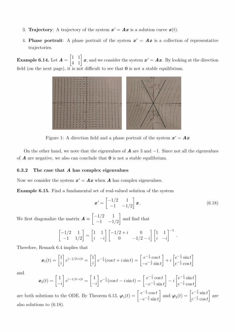
3. Trajectory: A trajectory of the system x 1 = Ax is a solution curve x(t).

4. Phase portrait: A phase portrait of the system x 1 = Ax is a collection of representativetrajectories.

Example 6.14. Let A =

[1 14 1

]x, and we consider the system x 1 = Ax. By looking at the direction

field (on the next page), it is not difficult to see that 0 is not a stable equilibrium.

Figure 1: A direction field and a phase portrait of the system x 1 = Ax

On the other hand, we note that the eigenvalues of A are 3 and ´1. Since not all the eigenvaluesof A are negative, we also can conclude that 0 is not a stable equilibrium.

6.3.2 The case that A has complex eigenvalues

Now we consider the system x 1 = Ax when A has complex eigenvalues.

Example 6.15. Find a fundamental set of real-valued solution of the system

x 1 =

[´1/2 1´1 ´1/2

]x . (6.18)

We first diagonalize the matrix A ”

[´1/2 1´1 ´1/2

]and find that

[´1/2 1´1 1/2

]=

[1 1i ´i

] [´1/2 + i 0

0 ´1/2 ´ i

] [1 1i ´i

]´1

.

Therefore, Remark 6.4 implies that

x1(t) =

[1i

]e(´1/2+i)t =

[1i

]e´ t

2 (cos t+ i sin t) =[e´ t

2 cos t´e´ t

2 sin t

]+ i

[e´ t

2 sin te´ t

2 cos t

]and

x2(t) =

[1

´i

]e(´1/2´i)t =

[1

´i

]e´ t

2 (cos t ´ i sin t) =[e´ t

2 cos t´e´ t

2 sin t

]´ i

[e´ t

2 sin te´ t

2 cos t

]are both solutions to the ODE. By Theorem 6.13, φ1(t) =

[e´ t

2 cos t´e´ t

2 sin t

]and φ2(t) =

[e´ t

2 sin te´ t

2 cos t

]are

also solutions to (6.18).

To see the linear independence of φ1 and φ2, we note that the Wronskian of φ1 and φ2 is

W(t) =

ˇ

ˇ

ˇ

ˇ

e´ t2 cos t e´ t

2 sin t´e´ t

2 sin t e´ t2 cos t

ˇ

ˇ

ˇ

ˇ

= e´t

which never vanishes. Therefore, tφ1,φ2u is a fundamental set of (6.18).Since det(A) ‰ 0, 0 is the only equilibrium. By looking at the direction field and phase portrait

of (6.18), we can image that 0 is a stable equilibrium.

Figure 2: The direction field and phase portrait of (6.18)

In fact, since φ1(t),φ2(t) Ñ 0 as t Ñ 8, any solution (which can be expressed as a linearcombination of φ1 and φ2) to (6.18) converges to 0 as t Ñ 8.

In general, if the constant matrix A has complex eigenvalues r˘ = λ ˘ iµ with correspondingeigenvectors u˘. Then

(A ´ r˘I)u˘ = 0 ô (A ´ Ďr˘I)Ďu˘ = 0 ô (A ´ r¯I)Ďu˘ = 0 .

Therefore, u´ could be chosen as the complex conjugate of u+. Let u+ = a+ ib and u´ = a ´ ib beeigenvectors associated with r+ and r´, respective, where a, b are real vectors. Let x1(t) = u+e

r+t

and x2(t) = a´er´t. Then x1,x2 are both solutions to x 1 = Ax since

x 11(t) = r+u+e

r+t = er+t(Au+) = Ax1(t) ,

x 12(t) = r´u´e

r´t = er´t(Au´) = Ax2(t) .

On the other hand, using the Euler identity we have

x1(t) = (a + ib)e(λ+iµ)t = (a + ib)eλt(cosµt+ i sinµt)= (a cosµt ´ b sinµt)eλt + i(a sinµt+ b cosµt)eλt ,

x2(t) = (a ´ ib)e(λ´iµ)t = (a ´ ib)eλt(cosµt ´ i sinµt)= (a cosµt ´ b sinµt)eλt ´ i(a sinµt+ b cosµt)eλt .

Therefore, Theorem 6.13 implies that φ1(t) ” (a cosµt ´ b sinµt)eλt and φ2(t) ” (a sinµt +b cosµt)eλt are also solutions to x 1 = Ax.

Now suppose that A is an n ˆ n matrix which has k distinct complex eigenvalues denoted byr(1)˘ , r

(2)˘ , ¨ ¨ ¨ , r

(k)˘ and n ´ 2k distinct real eigenvalues r2k+1, ¨ ¨ ¨ , rn with corresponding eigenvectors

u(1)˘ , u(2)

˘ , ¨ ¨ ¨ , u(k)˘ , u2k+1, ¨ ¨ ¨ ,uk, where

r (j)˘ = λj ˘ iµj for some λj, µj P R, and u(j)

+ =Ěu(j)

´ = a(j) + ib(j) .

Then the general solutions of x 1 = Ax is of the form

x(t) =kÿ

j=1

[C

(j)1

(a(j) cosµjt ´ b(j) sinµjt

)+ C

(j)2

(a(j) sinµjt+ b(j) cosµjt

)]eλjt +

nÿ

j=2k+1

Cjujeλjt .

If A is a 2 ˆ 2 matrix which has complex eigenvalues, then det(A) ‰ 0; thus 0 is the onlyequilibrium of the system x 1 = Ax. Now we check the stability of this equilibrium. Let u, v begiven as above. Then the Wronskian of u, v never vanishes. In fact,

W (u, v)(t)

=

ˇ

ˇ

ˇ

ˇ

(a1 cosµt ´ b1 sinµt)eλt (a1 sinµt+ b1 cosµt)eλt(a2 cosµt ´ b2 sinµt)eλt (a2 sinµt+ b2 cosµt)eλt

ˇ

ˇ

ˇ

ˇ

= e2λt[(a1 cosµt ´ b1 sinµt)(a2 sinµt+ b2 cosµt) ´ (a2 cosµt ´ b2 sinµt)(a1 sinµt+ b1 cosµt)

]= e2λt(a1b2 ´ a2b1) ‰ 0 ;

thus tu, vu is a linearly independent set. Moreover, Theorem 6.9 implies that every solution tox 1 = Ax can be expressed as a unique linear combination of u and v (thus every solution tox 1 = Ax can be expressed as a unique linear combination of φ1 and φ2). Therefore, we immediatelyfind that 0 is an asymptotically stable equilibrium if and only if λ ă 0.

Example 6.16. Consider the two-mass three-spring system

m1d2x1dt2

= ´(k1 + k2)x1 + k2x2 + F1(t) ,

m2d2x2dt2

= k2x1 ´ (k2 + k3)x2 + F2(t)

which is used to model the motion of two objects shown in the figure below.

Figure 3: A two-mass three-spring system

Letting y1 = x1, y2 = x2, y3 = x 11 and y4 = x 1

2, we find that y = (y1, y2, y3, y4)T satisfies

y 1 =

0 0 1 00 0 0 1

´k1 + k2m1

k2m1

0 0

k2m2

´k2 + k3m2

0 0

y +

00

F1(t)

m1F2(t)

m2

.

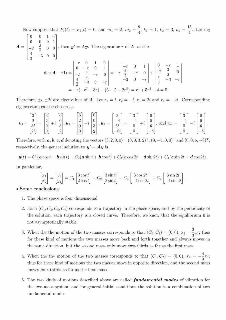
Now suppose that F1(t) = F2(t) = 0, and m1 = 2, m2 =9

4, k1 = 1, k2 = 3, k3 =

15

4. Letting

A =

0 0 1 00 0 0 1

´23

20 0

4

3´3 0 0

, then y 1 = Ay. The eigenvalue r of A satisfies

det(A ´ rI) =

ˇ

ˇ

ˇ

ˇ

ˇ

ˇ

ˇ

ˇ

ˇ

ˇ

´r 0 1 00 ´r 0 1

´23

2´r 0

4

3´3 0 ´r

ˇ

ˇ

ˇ

ˇ

ˇ

ˇ

ˇ

ˇ

ˇ

ˇ

= ´r

ˇ

ˇ

ˇ

ˇ

ˇ

ˇ

ˇ

´r 0 13

2´r 0

´3 0 ´r

ˇ

ˇ

ˇ

ˇ

ˇ

ˇ

ˇ

+

ˇ

ˇ

ˇ

ˇ

ˇ

ˇ

ˇ

0 ´r 1

´23

20

4

3´3 ´r

ˇ

ˇ

ˇ

ˇ

ˇ

ˇ

ˇ

= ´r(´r3 ´ 3r) + (6 ´ 2 + 2r2) = r4 + 5r2 + 4 = 0 .

Therefore, ˘i,˘2i are eigenvalues of A. Let r1 = i, r2 = ´i, r3 = 2i and r4 = ´2i. Correspondingeigenvectors can be chosen as

u1=

323i2i

=3200

+i0032

,u2 =

3200

´i

0032

,u3 =

3

´46i

´8i

=

3´400

+i

006

´8

, and u4 =

3

´400

´i

006

´8

.Therefore, with a, b, c,d denoting the vectors (3, 2, 0, 0)T, (0, 0, 3, 2)T, (3,´4, 0, 0)T and (0, 0, 6,´8)T,respectively, the general solution to y 1 = Ay is

y(t) = C1(a cos t ´ b sin t) + C2(a sin t+ b cos t) + C3(c cos 2t ´ d sin 2t) + C4(c sin 2t+ d cos 2t) .

In particular,[x1x2

]=

[y1y2

]= C1

[3 cos t2 cos t

]+ C2

[3 sin t2 sin t

]+ C3

[3 cos 2t

´4 cos 2t

]+ C4

[3 sin 2t

´4 sin 2t

].

‚ Some conclusions:

1. The phase space is four dimensional.

2. Each (C1, C2, C3, C4) corresponds to a trajectory in the phase space, and by the periodicity ofthe solution, each trajectory is a closed curve. Therefore, we know that the equilibrium 0 isnot asymptotically stable.

3. When the the motion of the two masses corresponds to that (C3, C4) = (0, 0), x2 =2

3x1; thus

for these kind of motions the two masses move back and forth together and always moves inthe same direction, but the second mass only move two-thirds as far as the first mass.

4. When the the motion of the two masses corresponds to that (C1, C2) = (0, 0), x2 = ´4

3x1;

thus for these kind of motions the two masses move in opposite direction, and the second massmoves four-thirds as far as the first mass.

5. The two kinds of motions described above are called fundamental modes of vibration forthe two-mass system, and for general initial conditions the solution is a combination of twofundamental modes.

6.3.3 The case that A has repeated eigenvalues

When A is diagonalizable, the discussion is pretty much the same as in the previous two sub-sections:if A = PΛP´1, then the solution to x 1 = Ax with initial data x(t0) = x0 can be written as

x(t) = P exp((t ´ t0)Λ)P´1x0 .

So we focus on the case that A is an nˆn matrix which is not diagonalizable. In this case, there mustbe at least one eigenvalue λ of A such that the dimension of the eigenspace

v P Cnˇ

ˇ (A´λI)v = 0(

is smaller than the algebraic multiplicity of λ.

Example 6.17. Let A =

[1 ´11 3

]and consider the system x 1 = Ax. We first compute the

eigenvalues (and the corresponding eigenvectors) and find that 2 is the only eigenvalue (with algebraicmultiplicity 2), while u = [1,´1]T is the only eigenvector associated with this eigenvalue. Therefore,A is not diagonalizable.

Let x = [x, y]T. Then x, y satisfy

x 1 = x ´ y , (6.19a)

y 1 = x+ 3y . (6.19b)

Using (6.19a) we obtain y = x ´ x 1; thus applying this identity to (6.19b) we find that x satisfies

x 1 ´ x 11 = x+ 3(x ´ x 1) or equivalently, x 11 ´ 4x 1 + 4x = 0 .

The characteristic equation to the ODE above is r2 ´ 4r + 4 = 0 (which should be the same as thecharacteristic equation for the matrix A); thus 2 is the only zero. From the discussion in Section3.4, we find that the solution to ODE (that x satisfies) is

x(t) = C1e2t + C2te

2t .

Using y = x ´ x 1, we find that the general solution to x 1 = Ax is

x =

[xy

]=

[C1e

2t + C2te2t

´(C1 + C2)e2t ´ C2te

2t

]= C1

[1

´1

]e2t + C2

[01

]e2t + C2

[1

´1

]te2t .

Letting v = [0, 1]T, we have x = (C1 + C2t)e2tu + C2e

2tv.

Given an large non-diagonalizable square matrix A, it is almost impossible to carry out the samecomputation as in Example 6.17, so we need to find another systematic way to find the solution tox 1 = Ax. The following theorem states that x(t) given by (6.16) is always the solution to x 1 = Axwith initial data x(t0) = x0, even if A is not diagonalizable.

Theorem 6.18. Let A be a square real constant matrix. Then the solution to x 1 = Ax with initialdata x(t0) = x0 is given by

x(t) = e(t´t0)Ax0 . (6.16)

Proof. Let y(t) = e(t´t0)Ax0. Then

y(t) =(

I + (t ´ t0)A +(t ´ t0)

2

2!A2 + ¨ ¨ ¨

)y0

= y0 + (t ´ t0)Ay0 +(t ´ t0)

2

2!A2y0 + ¨ ¨ ¨ +

(t ´ t0)k

k!Aky0 + ¨ ¨ ¨ .

Therefore,

y 1(t) = Ay0 + (t ´ t0)Ay0 + ¨ ¨ ¨ +(t ´ t0)

k´1

k!Aky0 + ¨ ¨ ¨

= A(

I + (t ´ t0)A +(t ´ t0)

2

2!A2 + ¨ ¨ ¨

)y0 = Ay

which implies that y is a solution to x 1 = Ax with initial data y(t0) = e0¨Ax0 = x0. By theuniqueness of the solution, we know that the solution to (6.12) with initial data x(t0) = x0 is givenby (6.16). ˝

Having established Theorem 6.18, we now focus on how to compute the exponential of a squarematrix if it is not diagonizable.

For a 2 ˆ 2 matrix A with repeated eigenvalue λ whose corresponding eigenvector is u (but notmore linearly independent eigenvector), by Example 6.17 we can conjecture that the general solutionto x 1 = Ax is

x(t) = (C1 + C2t)eλtu + C2e

λtv

for some unknown vector v. Now let us see what role v plays.Since x 1 = Ax, we must have

λ(C1 + C2t)eλtu + C2e

λtu + C2λeλtv = (C1 + C2t)e

λtAu + C2eλtAv .

By the fact that Au = λu and C2 is a general constant, the identity above implies that

u = (A ´ λI)v .

As a consequence, v satisfies (A ´ λI)2v = 0. Moreover, we must have v ∦ u (for otherwise u = 0)which implies that u, v are linearly independent.

Let P =[u ... v

], and Λ =

[λ 10 λ

]. Then AP = PΛ. Since u, v are linearly independent, P is

invertible; thusA = PΛP´1 .

Therefore, the same computations used in Section 6.3.1 shows that

e(t´t0)A = Pe(t´t0)ΛP´1 .

Finally, taking t0 = 0 (since the initial time could be translated to 0), then observing that

Λk =

[λk kλk´1

0 λk

], (6.20)

we conclude that

etΛ =8ÿ

k=0

tk

k!Λk =

8ř

k=0

tk

k!λk

8ř

k=1

tk

(k ´ 1)!λk´1

08ř

k=0

tk

k!λk

=

[eλt teλt

0 eλt

]. (6.21)

Having obtained the identity above, using (6.16) one immediately see that the general solution tox 1 = Ax is given by

x(t) =[u ... v

] [eλt teλt

0 eλt

] [C1

C2

].

In the following, we develop a general theory to compute e(t´t0)A for a square matrix A.

Definition 6.19. A square matrix A is said to be of Jordan canonical form if

A =

A1 O ¨ ¨ ¨ OO A2

. . . O... . . . . . . ...

O ¨ ¨ ¨ O Aℓ

, (6.22)

where each O is zero matrix, and each Ai is a square matrix of the form [λ] or

λ 1 0 ¨ ¨ ¨ ¨ ¨ ¨ ¨ ¨ ¨ 00 λ 1 0 ¨ ¨ ¨ ¨ ¨ ¨ 0... 0

. . . . . . 0 ¨ ¨ ¨...

... ... . . . . . . . . . 0...

... ... . . . . . . . . . 1 0

... ... . . . . . . 0 λ 10 ¨ ¨ ¨ ¨ ¨ ¨ ¨ ¨ ¨ ¨ ¨ ¨ 0 λ

for some eigenvalue λ of A.

We note that the diagonal elements of different Ai might be the same, and a diagonal matrix isof Jordan canonical form. Moreover, if A is of Jordan canonical form given by (6.22), then

Ak =

Ak

1 O ¨ ¨ ¨ OO Ak

2. . . O

... . . . . . . ...O ¨ ¨ ¨ O Ak

ℓ

and etA =

eA1 O ¨ ¨ ¨ OO eA2

. . . O... . . . . . . ...

O ¨ ¨ ¨ O eAℓ

. (6.23)

Example 6.20. Let Λ =

λ 0 00 λ 10 0 λ

. Then Λ is of Jordan canonical form, and using (6.20) and

(6.21) we conclude that

etΛ =

eλt 0 00 eλt teλt

0 0 eλt

.

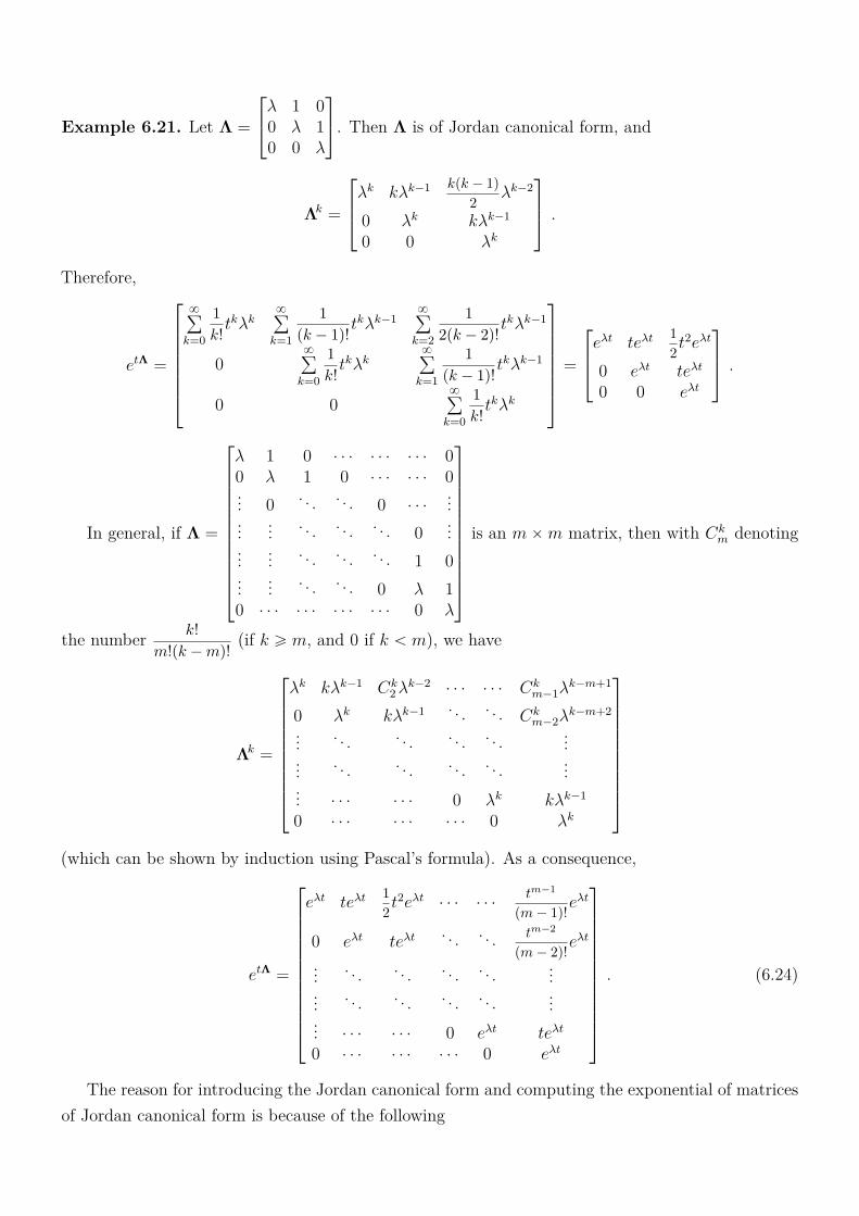
Example 6.21. Let Λ =

λ 1 00 λ 10 0 λ

. Then Λ is of Jordan canonical form, and

Λk =

λk kλk´1 k(k ´ 1)

2λk´2

0 λk kλk´1

0 0 λk

.

Therefore,

etΛ =

8ř

k=0

1

k!tkλk

8ř

k=1

1

(k ´ 1)!tkλk´1

8ř

k=2

1

2(k ´ 2)!tkλk´1

08ř

k=0

1

k!tkλk

8ř

k=1

1

(k ´ 1)!tkλk´1

0 08ř

k=0

1

k!tkλk

=

eλt teλt1

2t2eλt

0 eλt teλt

0 0 eλt

.

In general, if Λ =

λ 1 0 ¨ ¨ ¨ ¨ ¨ ¨ ¨ ¨ ¨ 00 λ 1 0 ¨ ¨ ¨ ¨ ¨ ¨ 0... 0

. . . . . . 0 ¨ ¨ ¨...

... ... . . . . . . . . . 0...

... ... . . . . . . . . . 1 0

... ... . . . . . . 0 λ 10 ¨ ¨ ¨ ¨ ¨ ¨ ¨ ¨ ¨ ¨ ¨ ¨ 0 λ

is an m ˆ m matrix, then with Ck

m denoting

the number k!

m!(k ´ m)!(if k ě m, and 0 if k ă m), we have

Λk =

λk kλk´1 Ck2λ

k´2 ¨ ¨ ¨ ¨ ¨ ¨ Ckm´1λ

k´m+1

0 λk kλk´1 . . . . . . Ckm´2λ

k´m+2

... . . . . . . . . . . . . ...

... . . . . . . . . . . . . ...

... ¨ ¨ ¨ ¨ ¨ ¨ 0 λk kλk´1

0 ¨ ¨ ¨ ¨ ¨ ¨ ¨ ¨ ¨ 0 λk

(which can be shown by induction using Pascal’s formula). As a consequence,

etΛ =

eλt teλt1

2t2eλt ¨ ¨ ¨ ¨ ¨ ¨

tm´1

(m ´ 1)!eλt

0 eλt teλt. . . . . . tm´2

(m ´ 2)!eλt

... . . . . . . . . . . . . ...

... . . . . . . . . . . . . ...

... ¨ ¨ ¨ ¨ ¨ ¨ 0 eλt teλt

0 ¨ ¨ ¨ ¨ ¨ ¨ ¨ ¨ ¨ 0 eλt

. (6.24)

The reason for introducing the Jordan canonical form and computing the exponential of matricesof Jordan canonical form is because of the following

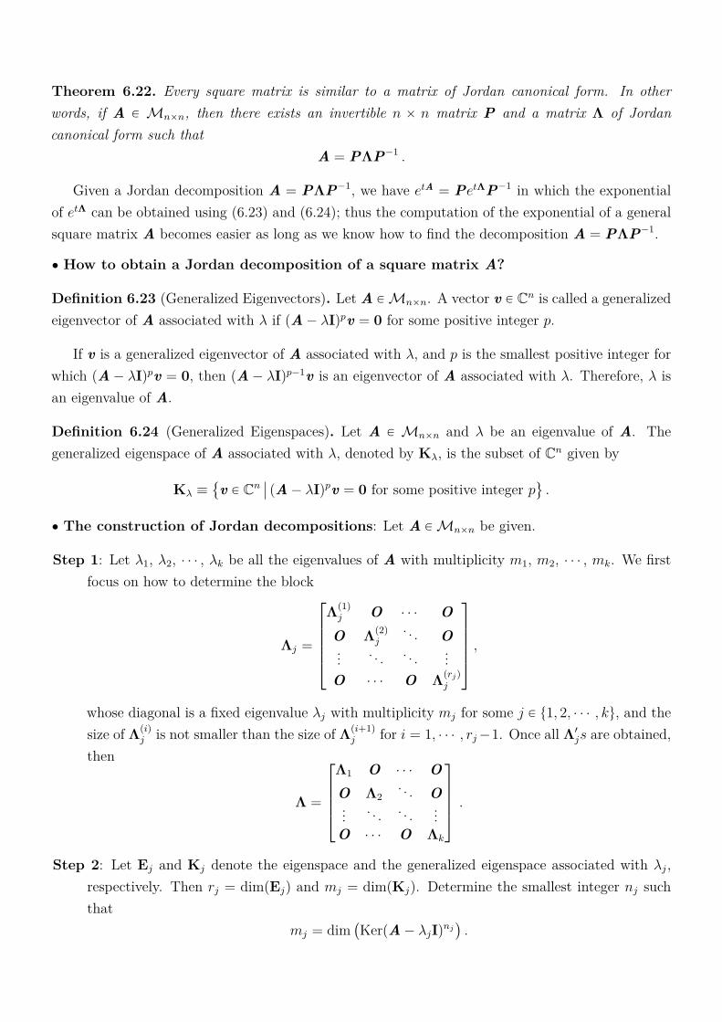
Theorem 6.22. Every square matrix is similar to a matrix of Jordan canonical form. In otherwords, if A P Mnˆn, then there exists an invertible n ˆ n matrix P and a matrix Λ of Jordancanonical form such that

A = PΛP´1 .

Given a Jordan decomposition A = PΛP´1, we have etA = PetΛP´1 in which the exponentialof etΛ can be obtained using (6.23) and (6.24); thus the computation of the exponential of a generalsquare matrix A becomes easier as long as we know how to find the decomposition A = PΛP´1.

‚ How to obtain a Jordan decomposition of a square matrix A?

Definition 6.23 (Generalized Eigenvectors). Let A P Mnˆn. A vector v P Cn is called a generalizedeigenvector of A associated with λ if (A ´ λI)pv = 0 for some positive integer p.

If v is a generalized eigenvector of A associated with λ, and p is the smallest positive integer forwhich (A ´ λI)pv = 0, then (A ´ λI)p´1v is an eigenvector of A associated with λ. Therefore, λ isan eigenvalue of A.

Definition 6.24 (Generalized Eigenspaces). Let A P Mnˆn and λ be an eigenvalue of A. Thegeneralized eigenspace of A associated with λ, denoted by Kλ, is the subset of Cn given by

Kλ ”

v P Cnˇ

ˇ (A ´ λI)pv = 0 for some positive integer p(

.

‚ The construction of Jordan decompositions: Let A P Mnˆn be given.

Step 1: Let λ1, λ2, ¨ ¨ ¨ , λk be all the eigenvalues of A with multiplicity m1, m2, ¨ ¨ ¨ , mk. We firstfocus on how to determine the block

Λj =

Λ

(1)j O ¨ ¨ ¨ O

O Λ(2)j

. . . O... . . . . . . ...

O ¨ ¨ ¨ O Λ(rj)j

,whose diagonal is a fixed eigenvalue λj with multiplicity mj for some j P t1, 2, ¨ ¨ ¨ , ku, and thesize of Λ(i)

j is not smaller than the size of Λ(i+1)j for i = 1, ¨ ¨ ¨ , rj ´1. Once all Λ1

js are obtained,then

Λ =

Λ1 O ¨ ¨ ¨ OO Λ2

. . . O... . . . . . . ...

O ¨ ¨ ¨ O Λk

.

Step 2: Let Ej and Kj denote the eigenspace and the generalized eigenspace associated with λj,respectively. Then rj = dim(Ej) and mj = dim(Kj). Determine the smallest integer nj suchthat

mj = dim(Ker(A ´ λjI)nj

).

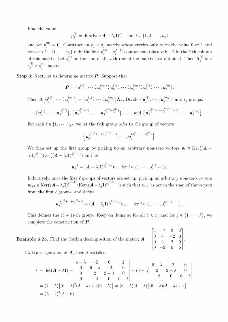
Find the valuep(ℓ)j = dim(Ker(A ´ λjI)ℓ

)for ℓ P t1, 2, ¨ ¨ ¨ , nju

and set p(0)j = 0. Construct an rj ˆ nj matrix whose entries only takes the value 0 or 1 andfor each ℓ P t1, ¨ ¨ ¨ , nju only the first p(ℓ)j ´ p

(ℓ´1)j components takes value 1 in the ℓ-th column

of this matrix. Let s(i)j be the sum of the i-th row of the matrix just obtained. Then Λ(i)j is a

s(i)j ˆ s

(i)j matrix.

Step 3: Next, let us determine matrix P. Suppose that

P =[u(1)

1

... ¨ ¨ ¨... u(m1)

1

... u(1)2

... ¨ ¨ ¨... u(m2)

2

... u(1)3

... ¨ ¨ ¨... u(n)

k

].

Then A[u(1)

j

... ¨ ¨ ¨... u(mj)

j

]=

[u(1)

j

... ¨ ¨ ¨... u(mj)

j

]Λj . Divide

u(1)j , ¨ ¨ ¨ ,u(mj)

j

(

into rj groups:

u(1)j , ¨ ¨ ¨ ,u(s

(1)j )

j

(

,

u(s(1)j +1)

j , ¨ ¨ ¨ ,u(s(1)j +s

(2)j )

j

(

, ¨ ¨ ¨ , and

u(s(1)j +¨¨¨+s

(rj´1)

j +1)

j , ¨ ¨ ¨ ,u(mj)j

(

.

For each ℓ P t1, ¨ ¨ ¨ , rju, we let the ℓ-th group refer to the group of vectors!

u(s(1)j +¨¨¨+s

(ℓ´1)j +1)

j , ¨ ¨ ¨ ,u(s(1)j +¨¨¨+s

(ℓ)j )

j

)

.

We then set up the first group by picking up an arbitrary non-zero vectors v1 P Ker((A ´

λjI)s(1)j zKer

((A ´ λjI)s

(1)j ´1

)and let

u(i)j = (A ´ λjI)s

(1)j ´iv1 for i P t1, ¨ ¨ ¨ , s

(1)j ´ 1u .

Inductively, once the first ℓ groups of vectors are set up, pick up an arbitrary non-zero vectorsvℓ+1 P Ker

((A´λjI)s

(ℓ+1)j zKer

((A´λjI)s

(ℓ+1)j ´1

)such that vℓ+1 is not in the span of the vectors

from the first ℓ groups, and define

u(s(1)j +¨¨¨+s

(ℓ)j +i)

j = (A ´ λjI)s(ℓ+1)j ´ivℓ+1 for i P t1, ¨ ¨ ¨ , s

(ℓ+1)j ´ 1u .

This defines the (ℓ + 1)-th group. Keep on doing so for all ℓ ď rj and for j P t1, ¨ ¨ ¨ , ku, wecomplete the construction of P.

Example 6.25. Find the Jordan decomposition of the matrix A =

4 ´2 0 20 6 ´2 00 2 2 00 ´2 0 6

.

If λ is an eigenvalue of A, then λ satisfies

0 = det(A ´ λI) =

ˇ

ˇ

ˇ

ˇ

ˇ

ˇ

ˇ

ˇ

4 ´ λ ´2 0 20 6 ´ λ ´2 00 2 2 ´ λ 00 ´2 0 6 ´ λ

ˇ

ˇ

ˇ

ˇ

ˇ

ˇ

ˇ

ˇ

= (4 ´ λ)

ˇ

ˇ

ˇ

ˇ

ˇ

ˇ

6 ´ λ ´2 02 2 ´ λ 0

´2 0 6 ´ λ

ˇ

ˇ

ˇ

ˇ

ˇ

ˇ

= (4 ´ λ)[(6 ´ λ)2(2 ´ λ) + 4(6 ´ λ)

]= (6 ´ λ)(4 ´ λ)

[(6 ´ λ)(2 ´ λ) + 4

]= (λ ´ 4)3(λ ´ 6) .

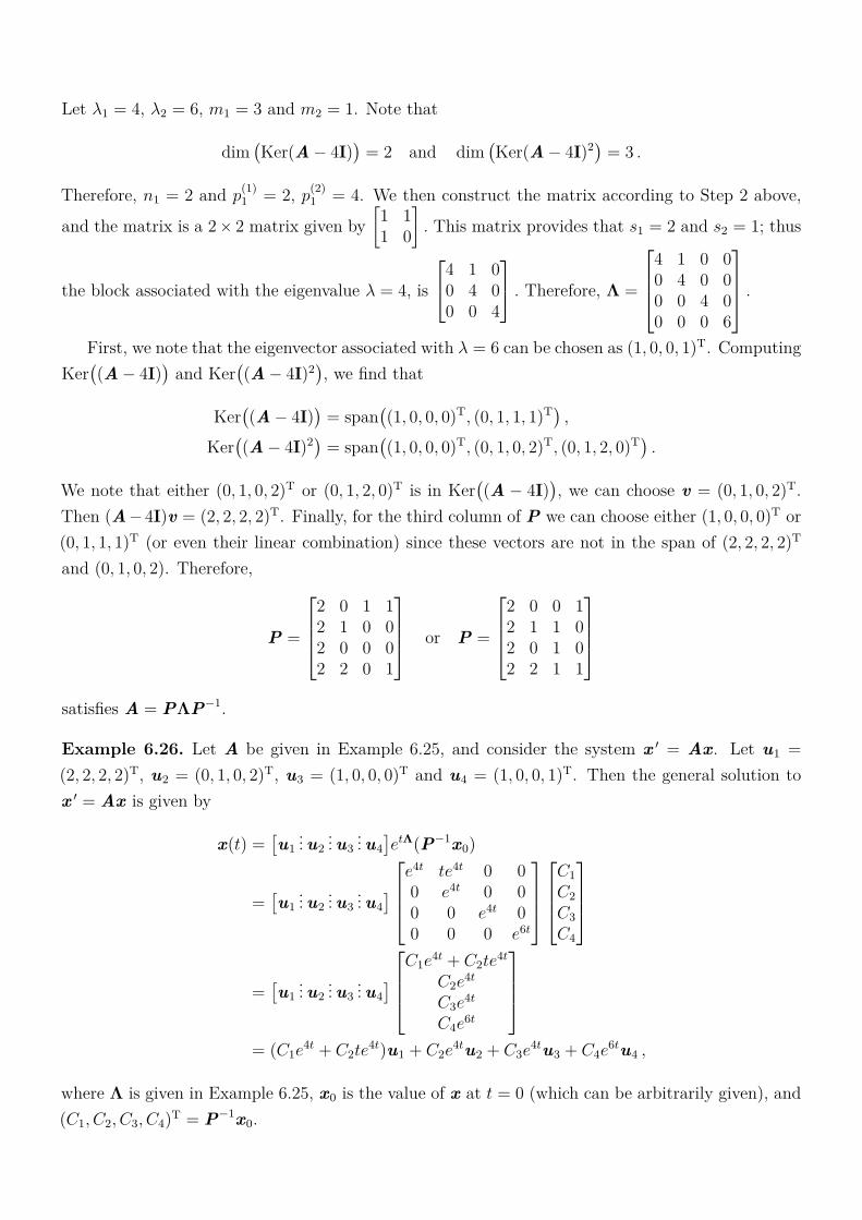
Let λ1 = 4, λ2 = 6, m1 = 3 and m2 = 1. Note that

dim(Ker(A ´ 4I)

)= 2 and dim

(Ker(A ´ 4I)2

)= 3 .

Therefore, n1 = 2 and p(1)1 = 2, p(2)1 = 4. We then construct the matrix according to Step 2 above,

and the matrix is a 2ˆ 2 matrix given by[1 11 0

]. This matrix provides that s1 = 2 and s2 = 1; thus

the block associated with the eigenvalue λ = 4, is

4 1 00 4 00 0 4

. Therefore, Λ =

4 1 0 00 4 0 00 0 4 00 0 0 6

.First, we note that the eigenvector associated with λ = 6 can be chosen as (1, 0, 0, 1)T. Computing

Ker((A ´ 4I)

)and Ker

((A ´ 4I)2

), we find that

Ker((A ´ 4I)

)= span

((1, 0, 0, 0)T, (0, 1, 1, 1)T) ,

Ker((A ´ 4I)2

)= span

((1, 0, 0, 0)T, (0, 1, 0, 2)T, (0, 1, 2, 0)T) .

We note that either (0, 1, 0, 2)T or (0, 1, 2, 0)T is in Ker((A ´ 4I)

), we can choose v = (0, 1, 0, 2)T.

Then (A ´ 4I)v = (2, 2, 2, 2)T. Finally, for the third column of P we can choose either (1, 0, 0, 0)T or(0, 1, 1, 1)T (or even their linear combination) since these vectors are not in the span of (2, 2, 2, 2)T

and (0, 1, 0, 2). Therefore,

P =

2 0 1 12 1 0 02 0 0 02 2 0 1

or P =

2 0 0 12 1 1 02 0 1 02 2 1 1

satisfies A = PΛP´1.

Example 6.26. Let A be given in Example 6.25, and consider the system x 1 = Ax. Let u1 =

(2, 2, 2, 2)T, u2 = (0, 1, 0, 2)T, u3 = (1, 0, 0, 0)T and u4 = (1, 0, 0, 1)T. Then the general solution tox 1 = Ax is given by

x(t) =[u1

... u2... u3

... u4

]etΛ(P´1x0)

=[u1

... u2... u3

... u4

] e4t te4t 0 00 e4t 0 00 0 e4t 00 0 0 e6t

C1

C2

C3

C4

=[u1

... u2... u3

... u4

] C1e

4t + C2te4t

C2e4t

C3e4t

C4e6t

= (C1e

4t + C2te4t)u1 + C2e

4tu2 + C3e4tu3 + C4e

6tu4 ,

where Λ is given in Example 6.25, x0 is the value of x at t = 0 (which can be arbitrarily given), and(C1, C2, C3, C4)

T = P´1x0.

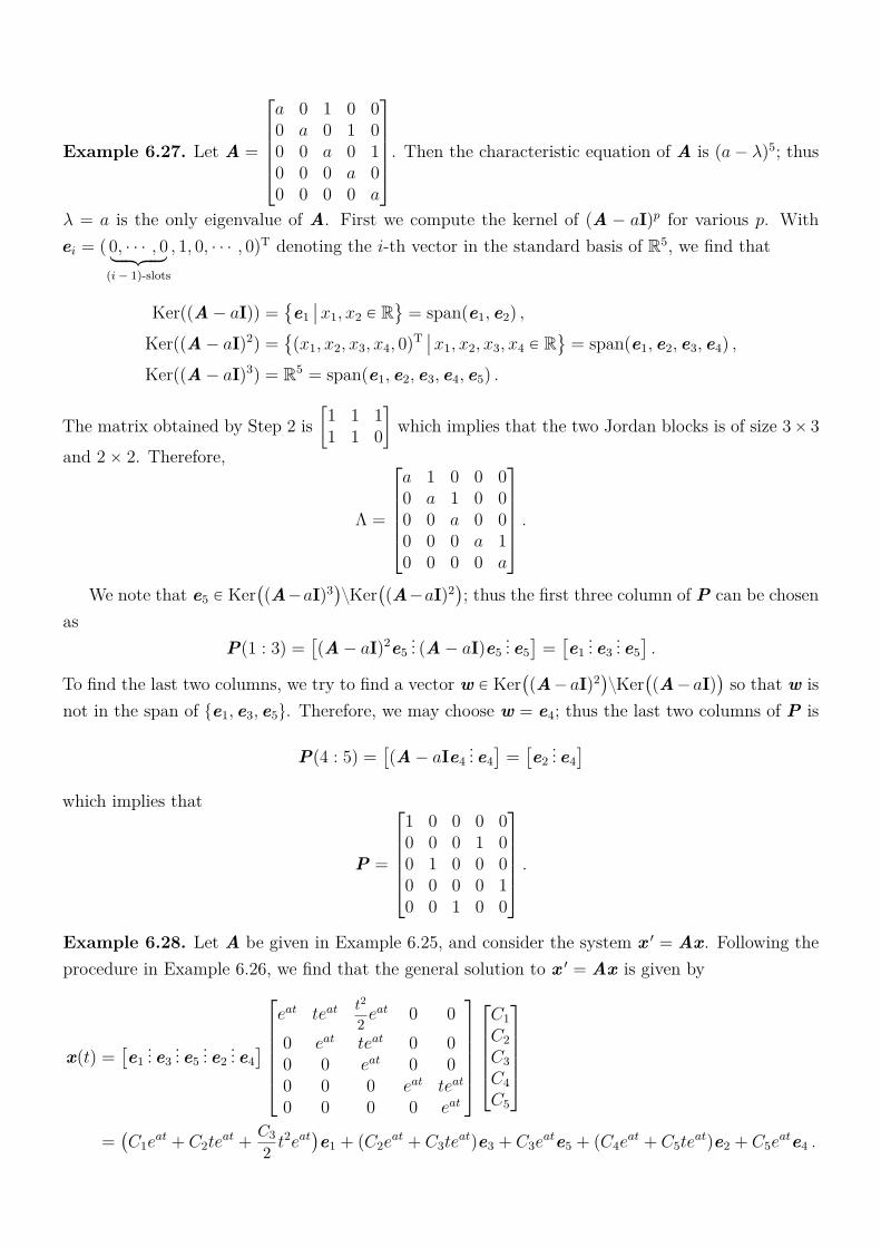
Example 6.27. Let A =

a 0 1 0 00 a 0 1 00 0 a 0 10 0 0 a 00 0 0 0 a

. Then the characteristic equation of A is (a ´ λ)5; thus

λ = a is the only eigenvalue of A. First we compute the kernel of (A ´ aI)p for various p. Withei = (0, ¨ ¨ ¨ , 0

looomooon

(i ´ 1)-slots

, 1, 0, ¨ ¨ ¨ , 0)T denoting the i-th vector in the standard basis of R5, we find that

Ker((A ´ aI)) =

e1

ˇ

ˇ x1, x2 P R(

= span(e1, e2) ,

Ker((A ´ aI)2) =

(x1, x2, x3, x4, 0)T ˇ

ˇx1, x2, x3, x4 P R(

= span(e1, e2, e3, e4) ,

Ker((A ´ aI)3) = R5 = span(e1, e2, e3, e4, e5) .

The matrix obtained by Step 2 is[1 1 11 1 0

]which implies that the two Jordan blocks is of size 3ˆ 3

and 2 ˆ 2. Therefore,

Λ =

a 1 0 0 00 a 1 0 00 0 a 0 00 0 0 a 10 0 0 0 a

.We note that e5 P Ker

((A´aI)3

)zKer

((A´aI)2

); thus the first three column of P can be chosen

asP(1 : 3) =

[(A ´ aI)2e5

... (A ´ aI)e5... e5

]=

[e1

... e3... e5

].

To find the last two columns, we try to find a vector w P Ker((A ´ aI)2

)zKer

((A ´ aI)

)so that w is

not in the span of te1, e3, e5u. Therefore, we may choose w = e4; thus the last two columns of P is

P(4 : 5) =[(A ´ aIe4

... e4

]=

[e2

... e4

]which implies that

P =

1 0 0 0 00 0 0 1 00 1 0 0 00 0 0 0 10 0 1 0 0

.Example 6.28. Let A be given in Example 6.25, and consider the system x 1 = Ax. Following theprocedure in Example 6.26, we find that the general solution to x 1 = Ax is given by

x(t) =[e1

... e3... e5

... e2... e4

]eat teat

t2

2eat 0 0

0 eat teat 0 00 0 eat 0 00 0 0 eat teat

0 0 0 0 eat

C1

C2

C3

C4

C5

=

(C1e

at + C2teat +

C3

2t2eat

)e1 + (C2e

at + C3teat)e3 + C3e

ate5 + (C4eat + C5te

at)e2 + C5eate4 .

6.4 Fundamental Matrices

In Definition 6.10 we have talked about the fundamental matrix of system x 1 = P(t)x. It is defined asa square matrix whose columns form an linearly independent set of solutions to the ODE x 1 = P(t)x.Let Ψ be a fundamental matrix of x 1 = P(t)x. Since each column of Ψ is a solution to the ODE,we must have

Ψ1(t) = P(t)Ψ(t) .

By the linearly independence of columns of Ψ, we must have

Ψ1(t)Ψ(t)´1 = P(t) for all t in the interval of interest. (6.25)

A special kind of fundamental matrix Φ, whose initial value Φ(t0) is the identity matrix, is inparticular helpful for constructing solutions to

x 1 = P(t)x , (6.26a)

x(t0) = x0 . (6.26b)

In fact, if Φ is a fundamental matrix of system x 1 = P(t)x satisfying Φ(t0) = I, then the solutionto (6.26) is given by

x(t) = Φ(t)x0 .

It should be clear to the readers that the i-th column of Φ is the solution to

x 1 = P(t)x ,

x(t0) = ei ,

where ei = (0, ¨ ¨ ¨ , 0looomooon

(i ´ 1)-slots

, 1, 0, ¨ ¨ ¨ , 0)T is the i-th vector in the standard basis of Rn (here we assume that

the size of P is n ˆ n). Moreover, for each fundamental matrix Ψ of (6.26a), we have the relation

Ψ(t) = Φ(t)Ψ(t0) .

Therefore, given a fundamental matrix Ψ, we can easily construct the fundamental matrix Φ(t) by

Φ(t) = Ψ(t)Ψ(t0)´1 .

Caution: Based on the discussions above and the information that the solution to the scalar equation

x1 = p(t)x with initial data x(t0) = x0 is x(t) = exp( ż t

t0

p(s) ds)x0, one might start guessing that

the solution to (6.26) is

x(t) = exp( ż t

t0

P(s) ds)

x0 . (6.27)

This is in fact NOT TRUE because in general P(s)P(t) ‰ P(t)P(s). Nevertheless, if P(s)P(t) =

P(t)P(s) for all s and t, then the solution to (6.26) is indeed given by (6.27). To see this, we firstnotice that

P(t)( ż t

t0

P(s) ds)=

ż t

t0

P(t)P(s) ds =

ż t

t0

P(s)P(t) ds =( ż t

t0

P(s) ds)

P(t) ;

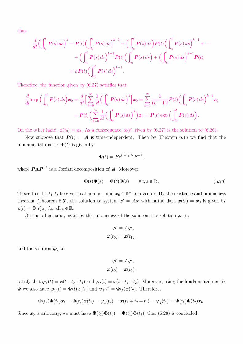
thus

d

dt

( ż t

t0

P(s) ds)k

= P(t)( ż t

t0

P(s) ds)k´1

+( ż t

t0

P(s) ds)

P(t)( ż t

t0

P(s) ds)k´2

+ ¨ ¨ ¨

+( ż t

t0

P(s) ds)k´2

P(t)( ż t

t0

P(s) ds)+( ż t

t0

P(s) ds)k´1

P(t)

= kP(t)( ż t

t0

P(s) ds)k´1

.

Therefore, the function given by (6.27) satisfies that

d

dtexp

( ż t

t0

P(s) ds)

x0 =d

dt

[ 8ÿ

k=0

1

k!

( ż t

t0

P(s) ds)k]

x0 =8ÿ

k=1

1

(k ´ 1)!P(t)

( ż t

t0

P(s) ds)k´1

x0

= P(t)( 8ÿ

k=0

1

k!

( ż t

t0

P(s) ds)k)

x0 = P(t) exp( ż t

t0

P(s) ds).

On the other hand, x(t0) = x0. As a consequence, x(t) given by (6.27) is the solution to (6.26).Now suppose that P(t) = A is time-independent. Then by Theorem 6.18 we find that the

fundamental matrix Φ(t) is given by

Φ(t) = Pe(t´t0)ΛP´1 ,

where PΛP´1 is a Jordan decomposition of A. Moreover,

Φ(t)Φ(s) = Φ(t)Φ(s) @ t, s P R . (6.28)

To see this, let t1, t2 be given real number, and x0 P Rn be a vector. By the existence and uniquenesstheorem (Theorem 6.5), the solution to system x 1 = Ax with initial data x(t0) = x0 is given byx(t) = Φ(t)x0 for all t P R.

On the other hand, again by the uniqueness of the solution, the solution φ1 to

φ 1 = Aφ ,

φ(t0) = x(t1) ,

and the solution φ2 to

φ 1 = Aφ ,

φ(t0) = x(t2) ,

satisfy that φ1(t) = x(t´ t0+ t1) and φ2(t) = x(t´ t0+ t2). Moreover, using the fundamental matrixΦ we also have φ1(t) = Φ(t)x(t1) and φ2(t) = Φ(t)x(t2). Therefore,

Φ(t2)Φ(t1)x0 = Φ(t2)x(t1) = φ1(t2) = x(t1 + t2 ´ t0) = φ2(t1) = Φ(t1)Φ(t2)x0 .

Since x0 is arbitrary, we must have Φ(t2)Φ(t1) = Φ(t1)Φ(t2); thus (6.28) is concluded.

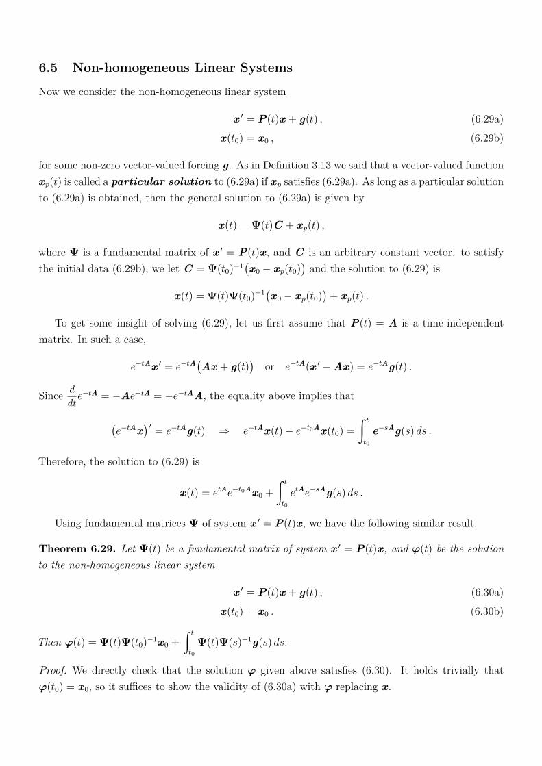
6.5 Non-homogeneous Linear Systems

Now we consider the non-homogeneous linear system

x 1 = P(t)x + g(t) , (6.29a)

x(t0) = x0 , (6.29b)

for some non-zero vector-valued forcing g. As in Definition 3.13 we said that a vector-valued functionxp(t) is called a particular solution to (6.29a) if xp satisfies (6.29a). As long as a particular solutionto (6.29a) is obtained, then the general solution to (6.29a) is given by

x(t) = Ψ(t)C + xp(t) ,

where Ψ is a fundamental matrix of x 1 = P(t)x, and C is an arbitrary constant vector. to satisfythe initial data (6.29b), we let C = Ψ(t0)

´1(x0 ´ xp(t0)

)and the solution to (6.29) is

x(t) = Ψ(t)Ψ(t0)´1(x0 ´ xp(t0)

)+ xp(t) .

To get some insight of solving (6.29), let us first assume that P(t) = A is a time-independentmatrix. In such a case,

e´tAx 1 = e´tA(Ax + g(t))

or e´tA(x 1 ´ Ax) = e´tAg(t) .

Since d

dte´tA = ´Ae´tA = ´e´tAA, the equality above implies that

(e´tAx

) 1= e´tAg(t) ñ e´tAx(t) ´ e´t0Ax(t0) =

ż t

t0

e´sAg(s) ds .

Therefore, the solution to (6.29) is

x(t) = etAe´t0Ax0 +

ż t

t0

etAe´sAg(s) ds .

Using fundamental matrices Ψ of system x 1 = P(t)x, we have the following similar result.

Theorem 6.29. Let Ψ(t) be a fundamental matrix of system x 1 = P(t)x, and φ(t) be the solutionto the non-homogeneous linear system

x 1 = P(t)x + g(t) , (6.30a)

x(t0) = x0 . (6.30b)

Then φ(t) = Ψ(t)Ψ(t0)´1x0 +

ż t

t0

Ψ(t)Ψ(s)´1g(s) ds.

Proof. We directly check that the solution φ given above satisfies (6.30). It holds trivially thatφ(t0) = x0, so it suffices to show the validity of (6.30a) with φ replacing x.

Differentiating φ and using (6.25), we find that

φ1(t) = Ψ1(t)Ψ(t0)´1x0 +Ψ(t)Ψ(t)´1g(t) +

ż t

t0

Ψ1(t)Ψ(s)´1g(s) ds

= Ψ1(t)Ψ(t)´1(Ψ(t)Ψ(t0)

´1x0 +

ż t

t0

Ψ(t)Ψ(s)´1g(s) ds)+ g(t)

= P(t)φ(t) + g(t)

which shows that φ satisfies (6.30a). ˝

‚ Another point of view - variation of parameters: Let Ψ be a fundamental matrix of x 1 = P(t)x.We look for a particular solution to x 1 = P(t)x + g(t). By the method of variation of parameterswe can assume that a particular solution can be expressed as

x(t) = Ψ(t)u(t)

for some vector-valued function u. Since x is a solution, we must have

Ψ1(t)u(t) +Ψ(t)u 1(t) = P(t)Ψ(t)u(t) + g(t) .

Since Ψ 1 = P(t)Ψ, we obtain that u satisfies

u 1(t) = Ψ(t)´1g(t) . (6.31)

Therefore, we can choose u(t) =ż

Ψ(t)´1g(t) dt and a particular solution to x 1 = P(t)x + g(t) isgiven by

xp(t) = Ψ(t)( ż

Ψ(t)´1g(t) dt). (6.32)

On the other hand, (6.31) implies that u(t) =ż t

t0

Ψ(s)´1g(s) ds+u(t0), where u(t0) is the value

of u at the initial time given by u(t0) = Ψ(t0)´1x(t0); thus the solution to x 1 = P(t)x + g(t) with

initial data x(t0) = x0 is

x(t) = Ψ(t)( ż t

t0

Ψ(s)´1g(s) ds+ u(t0))

= Ψ(t)Ψ(t0)´1x0 +

ż t

t0

Ψ(t)Ψ(s)´1g(s) ds .

Example 6.30. Let A =

[´2 11 ´2

]and g(t) =

[2e´t

3t

]. Find a particular solution of x 1 = Ax+g(t).

We first find the Jordan decomposition of A. The characteristic equation of A is (´2´r)2´1 = 0

which implies that λ = ´1 and λ = ´3 are eigenvalues of A. The corresponding eigenvectors are(1, 1)T and (1,´1)T; thus

A =

[1 11 ´1

] [´1 00 ´3

] [1 11 ´1

]T

;

thus

etA =

[1 11 ´1

] [e´t 00 e´3t

] [1 11 ´1

]T

.

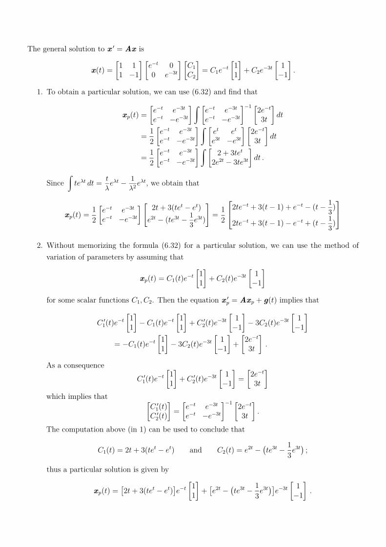
The general solution to x 1 = Ax is

x(t) =[1 11 ´1

] [e´t 00 e´3t

] [C1

C2

]= C1e

´t

[11

]+ C2e

´3t

[1

´1

].

1. To obtain a particular solution, we can use (6.32) and find that

xp(t) =

[e´t e´3t

e´t ´e´3t

]ż[e´t e´3t

e´t ´e´3t

]´1 [2e´t

3t

]dt

=1

2

[e´t e´3t

e´t ´e´3t

]ż[et et

e3t ´e3t

] [2e´t

3t

]dt

=1

2

[e´t e´3t

e´t ´e´3t

]ż[

2 + 3tet

2e2t ´ 3te3t

]dt .

Sinceż

teλt dt =t

λeλt ´

1

λ2eλt, we obtain that

xp(t) =1

2

[e´t e´3t

e´t ´e´3t

][ 2t+ 3(tet ´ et)

e2t ´ (te3t ´1

3e3t)

]=

1

2

2te´t + 3(t ´ 1) + e´t ´ (t ´1

3)

2te´t + 3(t ´ 1) ´ e´t + (t ´1

3)

2. Without memorizing the formula (6.32) for a particular solution, we can use the method of

variation of parameters by assuming that

xp(t) = C1(t)e´t

[11

]+ C2(t)e

´3t

[1

´1

]for some scalar functions C1, C2. Then the equation x 1

p = Axp + g(t) implies that

C 11(t)e

´t

[11

]´ C1(t)e

´t

[11

]+ C 1

2(t)e´3t

[1

´1

]´ 3C2(t)e

´3t

[1

´1

]= ´C1(t)e

´t

[11

]´ 3C2(t)e

´3t

[1

´1

]+

[2e´t

3t

].

As a consequence

C 11(t)e

´t

[11

]+ C 1

2(t)e´3t

[1

´1

]=

[2e´t

3t

]which implies that [

C 11(t)

C 12(t)

]=

[e´t e´3t

e´t ´e´3t

]´1 [2e´t

3t

].

The computation above (in 1) can be used to conclude that

C1(t) = 2t+ 3(tet ´ et) and C2(t) = e2t ´(te3t ´

1

3e3t

);

thus a particular solution is given by

xp(t) =[2t+ 3(tet ´ et)

]e´t

[11

]+[e2t ´

(te3t ´

1

3e3t

)]e´3t

[1

´1

].

6.6 Numerical Methods

So far we only talk about how to find a solution to x 1 = Ax+g(t) for constant matrix A. In general, itis very hard to compute (by hand) the general solution to x 1 = F(t,x) even if F(t,x) = P(t)x+g(t).In this section, we focus on solving the general system (6.8) numerically.

In the following discussion, we do not specify the size of the sysmte x 1 = F(t,x); thus n no longerdenote the length of the vector x.

Definition 6.31 (Informal definition). A numerical method of solving the ODE x 1 = F(t,x) withx(t0) = x0 is an iterative scheme which, when the step size h ą 0 is given, generates a uniquesequence of vectors tx1, ¨ ¨ ¨ ,xNu (for some N which in general depends on h) such that the piecewiselinear function φ satisfying

φ(t) =xn+1 ´ xn

h(t ´ tn) + xn @ t P [tn, tn+1] and n P t0, 1, ¨ ¨ ¨ , N ´ 1u ,

where tn = t0 + nh, resembles the solution to x 1 = F(t,x) with initial condition x(t0) = x0 in thetime interval [t0, tN ]. The function φ is called the numerical solution generated by this numericalmethod with step size h.

A numerical method of solving the ODE x 1 = F(t,x) is called a k-step method if it requiresxn,xn+1, ¨ ¨ ¨ ,xn+k´1 to determine xn+k for all n P t0, ¨ ¨ ¨ , N ´ ku. A numerical method of solvingthe ODE x 1 = F(t,x) is said to be explicit if it does not require “nonlinear procedures” to obtainsome xn’s, and is said to be implicit if it is not explicit.

Example 6.32. The forward Euler method of solving the ordinary differential equations y 1 = F(t,y)is an explicit one-step method given by

xn = xn´1 + hF(tn´1,xn´1) @n P t1, 2, ¨ ¨ ¨ , Nu ,

while the backward Euler method is an implicit one-step method given by

xn = xn´1 + hF(tn,xn) @n P t1, 2, ¨ ¨ ¨ , Nu .

Example 6.33. The Runge-Kutta method involves a weighted average of values of F(t,x) at differentpoints in the interval tn ď t ď tn+1, and is given by

xn+1 = xn + h(kn1 + 2kn2 + 2kn3 + kn4

6

), (6.33)

where

kn1 = F(tn,xn) , kn2 = F(tn +1

2h,xn +

1

2hkn1) ,

kn3 = F(tn +1

2h,xn +

1

2hkn2) , kn4 = F(tn + h,xn + hkn3) .

We note that the Runge-Kutta method is a one-step explicit method.

In this lecture we only consider explicit method.

Remark 6.34. A one-step explicit method is often (but not always) given in the form

xn+1 = xn + hΦ(tn,xn)

for some function Φ, while a k-step explicit method is often (but not always) given in the form

xn+1 = α1xn + α2xn´1 + ¨ ¨ ¨ + αkxn´k+1

+h[β1f(tn,xn) + β2f(tn´1,xn´1) + ¨ ¨ ¨ + βkf(tn´k+1,xn´k+1)

].

(6.34)

There are three fundamental sources of error of a numerical solution:

1. The iterative scheme used to produce the sequence tx1, ¨ ¨ ¨ ,xNu is an approximate one. Inother words, at each step the numerical method does not produce the correct value of thesolution at the next time step. This relates to the local/global truncation error.

2. The input data used in the iterative scheme are only approximations to the actual values ofthe solution at each tk. For example, one should use x(tk) to generate xk+1 but we are forcedto start with xk. This relates to the global truncation error.

3. The precision of calculations of the computer is finite. In other words, at each step only a finitenumber of digits can be retained. This relates to the round-off error (or machine error).

Definition 6.35. Let φ be a numerical solution obtained by a specific numerical method (with stepsize h ą 0 fixed) of solving ODE x 1 = F(t,x) with initial data x(t0) = x0. At each time step tn,

1. the global truncation error (associated with this numerical method) is the number En(h) =

x(tn) ´ φ(tn);

2. the local truncation error (associated with this numerical method) is the number τn(h) =

x(tn+1) ´ xn+1

h, where x(¨) is the exact solution and xn+1 is obtained according to the iterative

scheme with xj = x(tj) for all j P t0, 1, ¨ ¨ ¨ , nu.

3. the round-off error or machine error (associated with this numerical method) is thenumber Rn = φ(tn)´Xn, where Xn is the actual value computed from the numerical method.

In other words, the local truncation error measures the accuracy of the numerical method foreach time step, while the global truncation error measure the errors accumulated from the beginningof this iterative scheme.

Definition 6.36. A numerical method is said to be consistent if

limhÑ0

max0ďnďN´1

|τn(h)| = 0 ,

where τn(h) is the local truncation error associated with the numerical method with step size h.

Example 6.37. Consider the forward Euler method of solving x 1 = F(t,x). If x(t) is the solutionto x 1 = F(t,x) with initial data x(tn), then the Euler method provides an approximated value ofx(tn+1) given by

xn+1 = x(tn) + hF(tn,x(tn)

).

The local truncation error is then computed by

τn(h) =x(tn+1) ´ xn+1

h=

x(tn+1) ´ x(tn) ´ hF(tn,x(tn)

)h

=x(tn+1) ´ x(tn)

h´ F

(tn,x(tn)

)=

x(tn+1) ´ x(tn)h

´ x 1(tn) .

In other words, the local truncation τn(h) (of the forward Euler method) measures the differencebetween the real derivative and the “discrete derivative” (which allows us to design the numericalscheme).

Now consider the backward Euler method. Similar computation shows that the local truncationerror τn(h) associated with the backward Euler method is given by

τn(h) =x(tn+1) ´ x(tn)

h´ x 1(tn+1) .

Example 6.38. Consider the Runge-Kutta method given in Example 6.33. The local truncationerror τn(h) is given by

x(tn+1) ´ xn+1

h=

x(tn+1) ´ x(tn) + h(kn1 + 2kn2 + 2kn3 + kn4

6

)h

=x(tn+1) ´ x(tn)

h´kn1 + 2kn2 + 2kn3 + kn4

6,

where

kn1 = F(tn,x(tn)

), kn2 = F

(tn +

1

2h,x(tn) +

1

2hkn1

),

kn3 = F(tn +

1

2h,x(tn) +

1

2hkn2

), kn4 = F

(tn + h,x(tn) + hkn3

).

Assume that F is a scalar function (so that it is easy for the purpose of demonstration) and F is ofclass C 2 (that is, F is twice continuously differentiable). Then kn1 = x 1(tn), and

kn2 = F(tn,x(tn)

)+ F t

(tn,x(tn)

)h2+ Fx

(tn,x(tn)

)hkn12

+O(h2)

= x 1(tn) +h

2

[F t

(tn,x(tn)

)+ Fx

(tn,x(tn)

)kn1

]+O(h2) ,

kn3 = F(tn,x(tn)

)+ F t

(tn,x(tn)

)h2+ Fx

(tn,x(tn)

)hkn22

+O(h2)

= x 1(tn) +h

2

[F t

(tn,x(tn)

)+ Fx

(tn,x(tn)

)kn2

]+O(h2) ,

kn4 = F(tn,x(tn)

)+ F t

(tn,x(tn)

)h+ Fx

(tn,x(tn)

)hkn3 +O(h2)

= x 1(tn) + h[F t

(tn,x(tn)

)+ Fx

(tn,x(tn)

)kn3

]+O(h2) .

Therefore,

kn1 + 2kn2 + 2kn3 + kn46

= x 1(tn) +h

2F t

(tn,x(tn)

)+h

6Fx

(tn,x(tn)

)[x 1(tn) + kn2 + kn3

]+O(h2)

= x 1(tn) +h

2

[F t

(tn, x(tn)

)+ Fx

(tn, x(tn)

)x 1(tn)

]+O(h2)

= x 1(tn) +h

2x 11(tn) +O(h2)

which implies that

τn(h) =x(tn+1) ´ x(tn)

h´kn1 + 2kn2 + 2kn3 + kn4

6

=x(tn+1) ´ x(tn)

h´ x 1(tn) ´

h

2x 11(tn) +O(h2) .

Since F is of class C 2, x is of class C 3; thus the Taylor theorem implies that

x(tn+1) = x(tn) + hx 1(tn) +h2

2x 1(tn) +O(h3) .

As a consequence,

τn(h) =hx 1(tn) +

h2

2x 1(tn) +O(h3)

h´ x 1(tn) ´

h

2x 11(tn) +O(h2) = O(h2) .

Remark 6.39. If one assume that F is of class C 4, then the Runge-Kutta method provides numericalsolutions with local truncation error of order 4; that is, τn(h) = O(h4).

‚ Further look at the local truncation error and the consistency: Now we take a look atwhat the local truncation error for an one-step numerical scheme

xn+1 = xn + hΦ(h, tn,xn) (6.35)

really means. We remark that here Φ(h, tn,xn) can be viewed as a way to approximate the derivativein the time interval [tn, tn+1]. Moreover, both Euler method and Runge-Kutta scheme are one-stepmethods under this definition.

Before continuing the discussion, let us use the convention that for h ą 0 and fixed T ą 0, wedefine N =

[Th

]and the numerical solution φ generated by the one-step scheme (6.35) on the time

interval[tN , t0 + T ] (on which φ is not defined) has value φ(tN).

Suppose that there exists a unique solution x to (6.8) on the time interval [t0, t0+T ]. By definitionof the local truncation error,

τn(h) =x(tn+1) ´ xn+1

h=

x(tn+1) ´ x(tn)h

´ Φ(h, tn,x(tn)

)=

x(tn+1) ´ x(tn)h

´ x 1(tn) + F(tn,x(tn)

)+ Φ

(h, tn,x(tn)

).

If F is continuous on K ” [t0, t0 + T ] ˆ

[min

tP[t0,t0+T ]x(t), max

tP[t0,t0+T ]x(t)

], then x must be C 1 which

implies that x 1 is uniformly continuous on [t0, t0 + T ]. Therefore, the mean value theorem implies

thatlimhÑ0

max1ďnďN

ˇ

ˇ

ˇ

x(tn+1) ´ x(tn)h

´ x 1(tn)ˇ

ˇ

ˇ= 0 ;

thuslimhÑ0

max1ďnďN

|τn(h)| = limhÑ0

max1ďnďN

ˇ

ˇF(tn,x(tn)

)´ Φ

(h, tn,x(tn)

)ˇˇ . (6.36)

If we further assume the uniform continuity of Φ on its variables, then (6.36) further implies that

limhÑ0

max1ďnďN

|τn(h)| = limhÑ0

suptP[t0,t0+T ]

ˇ

ˇF(t,x(t)

)´ Φ

(h, t,x(t)

)ˇˇ (6.37)

Therefore, assuming that F is Lipchitz continuous (which guarantees the existence and uniquenessof the solution x to (6.8) by Theorem 6.5) and Φ is uniformly continuous, then the consistency of theone-step numerical scheme (6.35) is equivalent to that Φ

(h, ¨,x(¨)

)converges uniformly to F

(¨,x(¨)

)as h Ñ 0 (that is, (6.37)).

Remark 6.40. To see (6.36), let ε ą 0 and t P [t0, t0 + T ] be given. Since x 1 is continuous on[t0, t0 + T ], for some M ą 0 we have

ˇ

ˇx 1(t)ˇ

ˇ ď M for all t P [t0, t0 + T ]. Then

1. the uniform continuity of F provides a δ1 ą 0 such thatˇ

ˇF(t,y) ´ F(s, z)ˇ

ˇ ăε

2whenever (t,y), (s, z) P K satisfying |t ´ s|2 + |y ´ z|2 ă δ21 ;

2. the uniform continuity of Φ provides a δ2 ą 0 such thatˇ

ˇΦ(h, t,y) ´ Φ(h, s, z)ˇ

ˇ ăε

2whenever |t ´ s|2 + |y ´ z|2 ă δ22 .

Let δ =mintδ1, δ2u

M2 + 1. If 0 ă h ă δ, there exists tn such that |tn ´ t| ă δ. Therefore,

ˇ

ˇ

(tn,x(tn)

)´(

t,x(t))ˇˇ ă mintδ1, δ2u; thus

ˇ

ˇF(tn,x(tn)

)´ F

(t,x(t)

)ˇˇ+

ˇ

ˇΦ(h, tn,x(tn)

)´ Φ

(h, t,x(t)

)ˇˇ ă ε .

6.6.1 Convergence of Bounded Consistent Schemes

We first consider the convergence of numerical solutions obtained from a bounded (which is definedin Theorem 6.44) numerical scheme as the step size approaches zero.

Definition 6.41. Let a, b P R and a ă b. A family F of functions in C ([a, b];Rn) (which means foreach f P F , f : [a, b] Ñ Rn is a continuous vector-valued function) is said to be

1. uniformly bounded if

DM ą 0 Q |f(t)| ď M @ t P [a, b] and f P F ;

2. equi-continuous if

@ ε ą 0, D δ ą 0 Qˇ

ˇf(t) ´ f(s)ˇ

ˇ ă ε whenever |t ´ s| ă δ, t, s P [a, b], and k P N .

Now we introduce the Arzelà-Ascoli Theorem which can be applied to extract a uniformly con-vergent subsequence from a sequence of continuous functions as long as those functions are equi-continuous and uniformly bounded.

Theorem 6.42 (Arzelà-Ascoli). Let a, b P R with a ă b, and tfku8k=1 Ď C ([a, b];Rn) be a uniformly

bounded, equi-continuous sequence of functions. Then there exists a subsequence

fkj(8

j=1which

converges uniformly (to some function f P C ([a, b];Rn)).

Remark 6.43. The uniform convergence of the sequence tfku8k=1 to f on [a, b] means that

limkÑ8

supxP[a,b]

|fk(x) ´ f(x)| = 0 .

Theorem 6.44. For each h ą 0, let φh : [t0, t0 + T ] Ñ Rn be the numerical solution generated bythe one-step scheme (6.35) for some functions Φ. If Φ is bounded near h = 0; that is, there existsδ ą 0 and M ą 0 such that

ˇ

ˇΦ(h, t,x)ˇ

ˇ ď M for all (h, t,x) P (0, δ] ˆ [t0, t0 + T ] ˆ Rn, then everysubsequence

φhj

(8

j=1of tφhuhą0 possesses a uniformly convergent subsequence

φhjℓ

(8

ℓ=1; that is,

for some continuous function φ : [t0, t0 + T ] Ñ Rn, we have

limℓÑ8

suptP[t0,t0+T ]

ˇ

ˇφhjℓ(t) ´ φ(t)

ˇ

ˇ = 0 .

Proof. By Arzelà-Ascoli Theorem, it suffices to prove that the family of functions tφhuhą0 is uniformlybounded and equi-continuous.

First, since Φ is bounded by M , the numerical scheme implies thatˇ

ˇφh(tn)ˇ

ˇ ďˇ

ˇφh(tn´1)ˇ

ˇ+ hM ďˇ

ˇφh(tn´2)ˇ

ˇ+ 2hM ď ¨ ¨ ¨

ďˇ

ˇφh(0)ˇ

ˇ+ nhM ď |x0| +MT @n P

1, ¨ ¨ ¨ ,[Th

](.

Since φh are piecewise linear for all h ą 0, we find thatˇ

ˇφh(t)ˇ

ˇ ď |x0|eMT for all t P [t0, t0 + T ] and

for all h ą 0. Therefore, tφhuhą0 is a uniformly bounded family of continuous functions.On the other hand, by the boundedness of Φ again, we find that

ˇ

ˇ

ˇ

φh(t) ´ φh(s)

t ´ s

ˇ

ˇ

ˇď M @ t, s P [tn´1, tn] for some n P

1, ¨ ¨ ¨ ,[Th

](.

Therefore, by the fact thatˇ

ˇ

ˇ

φh(t) ´ φh(s)

t ´ s

ˇ

ˇ

ˇď max

!ˇ

ˇ

ˇ

φh(t) ´ φh(r)

t ´ r

ˇ

ˇ

ˇ,ˇ

ˇ

ˇ

φh(r) ´ φh(s)

r ´ s

ˇ

ˇ

ˇ

)

@ s ď r ď t ,

we find that tφhuhą0 is uniformly Lipschitz (with Lipschitz constant M) which implies that tφhuhą0

is an equi-continuous family of continuous functions. ˝

Therefore, every bounded numerical scheme produces a limit function which is a candidate ofthe exact solution. Next, we consider the convergence (to the exact solution) of numerical solutionsgenerated by a bounded consistent numerical scheme.

Theorem 6.45. Suppose that F : [t0, t0 + T ] ˆ Rn be uniformly continuous such that the system(6.8) has a unique solution x : [t0, t0 + T ] Ñ Rn. For each h ą 0, let φh : [t0, t0 + T ] Ñ Rn be thenumerical solution generated by the one-step scheme (6.35) for some functions Φ. If for some δ ą 0,Φ is bounded uniformly continuous on (0, δ]ˆ [t0, t0+T ]ˆRn, and Φ(h, ¨, ¨) converges to F uniformlyon [t0, t0 + T ] ˆ Rn as h Ñ 0, then the sequence tφhuhą0 converges uniformly to the exact solution xto (6.8).

Proof. If suffices to show that if the sequence

φhj

(8

j=1converges to some function φ uniformly on

[t0, t0 + T ], then φ must be the solution x to (6.8).Let ε ą 0 be given. Then the uniform continuity of Φ implies that there exists δ1 ą 0 such that

if |y ´ z| ă δ1, thensup

hą0,kPt0,¨¨¨ ,ℓu

ˇ

ˇΦ(h, kh,y

)´ Φ

(h, kh, z

)ˇˇ ă

ε

3T.

The uniform convergence of Φ(h, ¨, ¨) to F as h Ñ 0 implies that there exists δ2 ą 0 such that if0 ă h ă δ2,

sup(t,y)P(0,δ]ˆRn

ˇ

ˇF(t,y

)´ Φ

(h, t,y

)ˇˇ ă

ε

3T.

Moreover, since F(¨,φ(¨)

)is continuous on [t0, t0+T ], it is Riemann integrable over [t0, t0+T ]; thus

there exists δ3 ą 0 such that if 0 ă h ă δ3,

ˇ

ˇ

ˇ

ż t

t0

F(s,φ(s)

)ds ´

ℓ´1ÿ

k=0

F(t0 + kh,φ(t0 + kh))hˇ

ˇ

ˇăε

3.

Let t P [t0, t0 + T ] be given. For hj ą 0, we define ℓj =[ t

hj

]. Then φhj

satisfies that

φhj(t0 + hj) ´ φhj

(t0) = hjΦ(hj, t0,φhj

(t0)),

φhj(t0 + 2hj) ´ φhj

(t0 + hj) = hjΦ(hj, t0 + hj,φhj

(t0 + hj)),

... =...

φhj

(tℓj ´ hj

)´ φhj

(tℓj ´ 2hj) = hjΦ(hj, t0 + (ℓj ´ 2)hj,φhj

(t0 + (ℓj ´ 2)hj)),

φhj(tℓj) ´ φhj

(tℓj ´ hj) = hjΦ(hj, t0 + (ℓj ´ 1)hj,φhj

(t0 + (ℓj ´ 1)hj)).

Summing all the equalities, we find that

φhj(tℓj) = φhj

(t0) +

ℓj´1ÿ

k=0

Φ(hj, t0 + khj,φhj(t0 + khj)

)hj

= x0 +

ℓj´1ÿ

k=0

Φ(hj, t0 + khj,φhj(t0 + khj)

)hj . (6.38)

Now, by the uniform convergence of

φhj

(8

j=1and hj Ñ 0 as j Ñ 8, there exists N ą 0 such

that if j ě N ,suptP[0,T ]

ˇ

ˇφhj(t) ´ φ(t)

ˇ

ˇ ă δ1 and 0 ă hj ă mintδ2, δ3u .

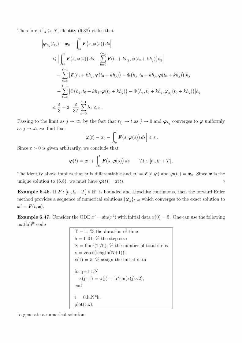
Therefore, if j ě N , identity (6.38) yields thatˇ

ˇ

ˇφhj

(tℓj) ´ x0 ´

ż t

t0

F(s,φ(s)

)dsˇ

ˇ

ˇ

ď

ˇ

ˇ

ˇ

ż t

t0

F(s,φ(s)

)ds ´

ℓ´1ÿ

k=0

F(t0 + khj,φ(t0 + khj))hj

ˇ

ˇ

ˇ

+ℓ´1ÿ

k=0

ˇ

ˇF(t0 + khj,φ(t0 + khj))

´ Φ(hj, t0 + khj,φ(t0 + khj)

)ˇˇhj

+ℓ´1ÿ

k=0

ˇ

ˇΦ(hj, t0 + khj,φ(t0 + khj)

)´ Φ

(hj, t0 + khj,φhj

(t0 + khj))ˇˇhj

ďε

3+ 2 ¨

ε

3T

ℓ´1ÿ

k=0

hj ď ε .

Passing to the limit as j Ñ 8, by the fact that tℓj Ñ t as j Ñ 0 and φhjconverges to φ uniformly

as j Ñ 8, we find thatˇ

ˇ

ˇφ(t) ´ x0 ´

ż t

t0

F(s,φ(s)

)dsˇ

ˇ

ˇď ε .

Since ε ą 0 is given arbitrarily, we conclude that

φ(t) = x0 +

ż t

t0

F(s,φ(s)

)ds @ t P [t0, t0 + T ] .

The identity above implies that φ is differentiable and φ 1 = F(t,φ) and φ(t0) = x0. Since x is theunique solution to (6.8), we must have φ(t) = x(t). ˝

Example 6.46. If F : [t0, t0 + T ]ˆRn is bounded and Lipschitz continuous, then the forward Eulermethod provides a sequence of numerical solutions tφhuhą0 which converges to the exact solution tox 1 = F(t,x).

Example 6.47. Consider the ODE x 1 = sin(x2) with initial data x(0) = 5. One can use the followingmatlabr code

T = 1; % the duration of timeh = 0.01; % the step sizeN = floor(T/h); % the number of total stepsx = zeros(length(N+1));x(1) = 5; % assign the initial data

for j=1:1:Nx(j+1) = x(j) + h*sin(x(j)^2);

end

t = 0:h:N*h;plot(t,x);

to generate a numerical solution.

6.6.2 The Rate of Convergence

In this sub-section, we focus on how fast a sequence of numerical solutions converges to the exactsolution (given that the assumptions in Theorem 6.45 and probably more assumptions hold). To seethe rate of convergence, we have to look at the convergence behavior of the global truncation error.

By the mean value theorem (for functions of several variables),

En(h) = x(tn) ´ xn = x(tn) ´ xn´1 ´ hΦ(h, tn´1,xn´1)

= x(tn) ´ x(tn´1) ´ hΦ(h, tn´1,x(tn´1)) + x(tn´1) ´ xn´1

+ h[Φ(h, tn´1,x(tn´1)) ´ Φ(h, tn´1,xn´1)

]= hτ n´1(h) + En´1(h) + h(∇xΦ)(h, tn´1, ξn´1)

[x(tn´1) ´ xn´1

]= hτ n´1(h) + En´1(h) + h(∇xΦ)(h, tn´1, ξn´1)En´1(h)

for some ξn´1 on the line segment joining x(tn´1) and xn´1. If we assume thatˇ

ˇ∇xΦˇ

ˇ is bounded byK, then the equality above implies that

|En(h)| ď h|τ n´1(h)| + (1 + hK)|En´1(h)| .

Therefore,

|En(h)| ď h|τ n´1(h)| + (1 + hK)|En´1(h)| ,

(1 + hK)|En´1(h)| ď h(1 + hK)|τ n´2(h)| + (1 + hK)2|En´2(h)| ,

... ď...

(1 + hK)n´1|E1(h)| ď h(1 + hK)n´1|τ 0(h)| + (1 + hK)n|E0(h)| .

Summing all the inequalities above, we find that

|En(h)| ď hnÿ

k=1

(1 + hK)k´1ˇ

ˇτ n´k(h)ˇ

ˇ+ (1 + hK)n|E0(h)| . (6.39)

Suppose that the local truncation error satisfies

|τ n(h)| ď Ahr @n P

0, 1, ¨ ¨ ¨ ,[Th

]´ 1

(

for some constant A and r ą 0. Then by the fact E0(h) = 0, we conclude that

|En(h)| ď hnÿ

k=1

(1 + hK)k´1Ahr + (1 + hK)n|E0(h)| ď h(1 + hK)n ´ 1

hKAhr

ď1

K

[(1 + hK)

Th ´ 1

]Ahr ď

1

K(eKT ´ 1)Ahr .

Therefore, we establish the following

Theorem 6.48. Assume the conditions in Theorem 6.45. If ∇xΦ is bounded by K and the localtruncation error τ n(h) satisfies

|τ n(h)| ď Ahr @n P

0, 1, ¨ ¨ ¨ ,[Th

]´ 1

(

and h ą 0

for some constant A ą 0, then the global truncation error En(h) satisfies

|En(h)| ď1

K(eKT ´ 1)hr @h ą 0 .

Example 6.49. If F : [t0, t0 + T ]ˆRn is bounded and Lipschitz continuous, then the forward Eulermethod provides a sequence of numerical solutions tφhuhą0 which converges to the exact solution tox 1 = F(t,x) with rate

suptP[t0,t0+T ]

ˇ

ˇφh(t) ´ x(t)ˇ

ˇ ď Ch @h ą 0

for some constant C ą 0. To see this, we first note that Theorem 6.48 implies that there existsM ą 0 such that

sup0ďnď[T/h]

ˇ

ˇφh(tn) ´ x(tn)ˇ

ˇ ď Mh @h ą 0 .

Suppose that |F | is bounded by L. For t P [t0, t0 + T ], choose n P t0, 1, ¨ ¨ ¨ , N ´ 1u such thattn ď t ď tn+1. Then

ˇ

ˇφh(t) ´ φh(tn)ˇ

ˇ ďˇ

ˇφh(tn+1) ´ φh(tn)ˇ

ˇ = hˇ

ˇF(tn,φh(tn)

)ˇˇ ď Lh

and the mean value theorem implies thatˇ

ˇx(t) ´ x(tn)ˇ

ˇ ďˇ

ˇx 1(ξ)ˇ

ˇ|t ´ tn| =ˇ

ˇF(ξ,x(ξ)

)ˇˇ|t ´ tn| ď Lh .

Therefore,ˇ

ˇx(t) ´ φh(t)ˇ

ˇ ďˇ

ˇx(t) ´ x(tn)ˇ

ˇ+ˇ

ˇx(tn) ´ φh(tn)ˇ

ˇ+ˇ

ˇφh(tn) ´ φh(t)ˇ

ˇ ď (M + 2L)h @h ą 0 .

7 The Laplace Transform

7.1 Definition of the Laplace Transform

Definition 7.1 (Integral transform). An integral transform is a relation between two functionsf and F of the form

F (s) =

ż β

α

K(s, t)f(t) dt , (7.1)

where K(¨, ¨) is a given function, called the kernel of the transformation, and the limits of integrationα, β are also given (here α, β could be 8 and in such cases the integral above is an improper integral).The relation (7.1) transforms function f into another function F called the transformation of f .

Proposition 7.2. Every integral transform is linear; that is, for all functions f and g (defined on(α, β)) and constant a,

ż β

α

K(s, t)(af(t) + g(t)

)dt = a

ż β

α

K(s, t)f(t) dt+

ż β

α

K(s, t)g(t) dt .

Example 7.3. Let f : R Ñ R be a function such thatż 8

´8

|f(x)| dx ă 8. The Fourier transform

of f , denoted by F (f), is defined by

F (f)(s) =1

?2π

ż 8

´8

e´istf(t) dt(= lim

α,βÑ8

ż β

´α

e´istf(t)dt),

where the kernel K is a complex function (i.e., the value of K is complex). We will discuss theFourier transform later.

Definition 7.4 (Laplace transform). Let f : [0,8] Ñ R be a function. The Laplace transformof f , denoted by L (f), is defined by

L (f)(s) =

ż 8

0

e´stf(t) dt(= lim

RÑ8

ż R

0

e´istf(t)dt),

provided that the improper integral exists.

Example 7.5. Let f : [0,8) Ñ R be defined by f(t) = eat, where a P R is a constant. Since theimproper integral

ż 8

0

e(a´s)t dt = limRÑ8

ż R

0

e(a´s)t dt(s‰a)= lim

RÑ8

(´

e(a´s)t

(s ´ a)

ˇ

ˇ

ˇ

t=R

t=0

)= lim

RÑ8

1 ´ e(a´s)R

s ´ a

exists for s ą a, we find thatL (f)(s) =

1

s ´ a@ s ą a .

Example 7.6. Let f : [0,8) Ñ R be defined by

f(t) =

$

’

&

’

%

1 if 0 ď t ă 1 ,

k if t = 1 ,

0 if t ą 1 ,

where k is a given constant. Since the improper integralż 8

0

e´stf(t) dt =

ż 1

0

e´stdt =1 ´ e´s

s

exists as long as s ‰ 0, we find that

L (f)(s) =1 ´ e´s

s@ s ‰ 0 .

We note that the Laplace transform in this case is independent of the choice of k; thus the Laplacetransform is not one-to-one (in the classical/pointwise sense).

Example 7.7. Let f : [0,8) Ñ R be given by f(t) = sin(at). Note thatż R

0

e´stloomoon

”u

sin(at) dtlooomooon

”dv

= ´e´st cos(at)a

ˇ

ˇ

ˇ

t=R

t=0+

ż R

0

(´s)e´st cos(at)a

dt

=1

a

(1 ´ e´Rs cos(aR)

)´s

a

ż R

0

e´st cos(at) dt (7.2)

=1

a

(1 ´ e´Rs cos(aR)

)´s

a

(e´st sin(at)

a

ˇ

ˇ

ˇ

t=R

t=0+s

a

ż R

0

e´st sin(at) dt)

=1

a

(1 ´ e´Rs cos(aR)

)´

s

a2e´Rs sin(aR) ´

s2

a2

ż R

0

e´st sin(at) dt ;

thus we obtain that(1 +

s2

a2

) ż R

0

e´st sin(at) dt = 1

a

(1 ´ e´Rs cos(aR)

)´

s

a2e´Rs sin(aR) .

Therefore, the improper integralż 8

0

e´st sin(at) dt = limRÑ8

ż R

0

e´st sin(at) dt

= limRÑ8

[ a

s2 + a2

(1 ´ e´Rs cos(aR)

)´

s

s2 + a2e´Rs sin(aR)

]exists for all s ą 0 which implies that

L (f)(s) =a

s2 + a2@ s ą 0 .

Moreover, (7.2) further implies thatż 8

0

e´st cos(at) dt = a

s

(1a

´a

s2 + a2

)=

s

s2 + a2.

Proposition 7.8. Suppose that

1. f is piecewise continuous on the interval 0 ď t ď R for all positive R P R;

2. f is of exponential order a; that is, |f(t)| ď Meat for some M and a.

Then the Laplace transform of f exists for s ą a.

Proof. Since f is piecewise continuous on [0, R], the integralż R

0e´stf(t) dt exists. If 0 ă R1 ă R2,

by the fact that |f(t)| ď Meat for some M and a, we find thatˇ

ˇ

ˇ

ż R2

R1

e´stf(t) dtˇ

ˇ

ˇď

ż R2

R1

e´stMeat dt =Me(a´s)R2 ´ e(a´s)R1

a ´ s

which converges to 0 as R1, R2 Ñ 8 if s ą a. Therefore, the improper integralż 8

0e´stf(t) dt exists.

˝

Example 7.9. Let f : [0,8) Ñ R be given by f(t) = tp for some p ą ´1. Recall that the Gammafunction Γ : (0,8) Ñ R is defined by

Γ(x) =

ż 8

0

e´ttx´1 dt .

We note that if ´1 ă p ă 0, f is not of exponential order a for all a P R; however, the Laplacetransform of f exists the Laplace transform of f exists. In fact, for s ą 0,

L (f)(s) = limRÑ8

ż R

0

e´sttp dt = limRÑ8

ż sR

0

e´t( ts

)pdt

s=

Γ(p+ 1)

sp+1.

In particular, if p = n P N Y t0u, then

L (f)(s) =n!

sn+1@ s ą 0 .

7.1.1 The Inverse Laplace Transform

Even though Example 7.6 shows that the Laplace transform is not one-to-one in the classical sense,we are still able to talk about the “inverse” of the Laplace transform because of the following

Theorem 7.10 (Lerch). Suppose that f, g : [0,8) Ñ R are continuous and of exponential order a.If L (f)(s) = L (g)(s) for all s ą a, then f(t) = g(t) for all t ě 0.

Remark 7.11. The inverse Laplace transform of a function F is given by

L ´1(F )(t) =1

2πilimRÑ8

ż γ+iR

γ´iR

estF (s) ds ,

where the integration is done along the vertical line Re(s) = γ in the complex plane such that γ isgreater than the real part of all singularities of F .

7.2 Solution of Initial Value Problems

Theorem 7.12. Suppose that f : [0,8) Ñ R is continuous with piecewise continuous derivative,and f is of exponential order a. Then the Laplace transform of f 1 exist for s ą a, and

L (f 1)(s) = sL (f)(s) ´ f(0) .

Proof. Since f is of exponential order, the Laplace transform of f exists. Since f is continuous,integrating by parts we find that

ż R

0

e´stf 1(t) dt = e´stf(t)ˇ

ˇ

ˇ

t=R

t=0´

ż R

0

(´s)e´stf(t) dt = e´Rsf(R) ´ f(0)s

ż R

0

e´stf(t) dt .

Since f is of exponential order a, e´Rsf(R) Ñ 0 as s Ñ 8; thus

L (f 1)(s) = limRÑ8

ż R

0

e´stf 1(t) dt = ´f(0) + s limRÑ8

ż R

0

e´stf(t) dt = sL (f)(s) ´ f(0) . ˝

Corollary 7.13. Suppose that f : [0,8) Ñ R is a function such that f, f 1, f 11, ¨ ¨ ¨ , f (n´1) are contin-uous of exponential order a, and f (n) is piecewise continuous. Then L (f (n)(s) exists for all s ą a,and

L (f (n))(s) = snL (f)(s) ´ sn´1f(0) ´ sn´2f 1(0) ´ ¨ ¨ ¨ ´ sf (n´2)(0) ´ f (n´1)(0) .

Example 7.14. Consider the ODEy 11 ´ y 1 ´ 2y = 0 .

If the solution y and its derivative y 1 are of exponential order a for some a P R, then by taking theLaplace transform of the equation above we find that[

s2L (y) ´ sy(0) ´ y 1(0)]

´[sL (y) ´ y(0)

]´ 2L (y) = 0 ;

thus

L (y)(s) =sy(0) + y 1(0) ´ y(0)

s2 ´ s ´ 2=sy(0) + y 1(0) ´ y(0)

(s ´ 2)(s+ 1)

=y(0)

s+ 1+

y 1(0) + y(0)

(s ´ 2)(s+ 1)=

y(0)

s+ 1+y 1(0) + y(0)

3

( 1

s ´ 2´

1

s+ 1

).

By Example 7.5 and Theorem 7.10, we find that

y(t) = y(0)e´t +y 1(0) + y(0)

3

(e2t ´ e´t

).

The procedure listed in Example 7.14 provides a way of solving of an ODE with constant coeffi-cients. In fact, suppose that we are looking for solutions to

y 11 + by 1 + cy = f(t) .

Then taking the Laplace transform of the equation above (here we assume that y and y 1 are ofexponential order a for some a P R), we find that

s2L (y)(s) ´ sy(0) ´ y 1(0) + b(sL (y)(s) ´ y(0)

)+ cL (y)(s) = L (f)(s)

which implies that the Laplace transform of the solution y satisfies

L (y)(s) =(s+ b)y(0) + y 1(0)

s2 + bs+ c+

L (f)(s)

s2 + bs+ c. (7.3)

The ODE is then solved provided that we can find the function y = φ(t) whose Laplace transform isthe right-hand side of (7.3).

Example 7.15. Find the solution of the ODE y 11 + y = sin 2t with initial condition y(0) = 2 andy 1(0) = 1. If y is the solution to the ODE and y, y 1 are of exponential order a for some a P R, then(7.3) and Example 7.7 imply that the Laplace transform of y is given by

L (y)(s) =2s+ 1

s2 + 1+

2

(s2 + 1)(s2 + 4).

Using partial fractions, we expect that

2

(s2 + 1)(s2 + 4)=as+ b

s2 + 1+cs+ d

s2 + 4=

(a+ c)s3 + (b+ d)s2 + (4a+ c)s+ (4b+ d)

(s2 + 1)(s2 + 4).

Therefore, a+ c = b+ d = 4a+ c = 0 and 4b+ d = 2; thus a = c = 0 and b = ´d =2

3. This provides

thatL (y)(s) =

2s+ 1

s2 + 1+

2

3

1

s2 + 1´

2

3

1

s2 + 4=

2s

s2 + 1+

5

3

1

s2 + 1´

1

3

2

s2 + 4.

By Proposition 7.2 and Example 7.7, we find that

y(t) = 2 cos t+ 5

3sin t ´

1

3sin 2t .

Example 7.16. Find the solution of the ODE y(4) ´ y = 0 with initial condition y(0) = y 11(0) =

y 12(0) = 0 and y 1(0) = 1 and y, y 1 are of exponential order a for some a P R. If y is the solution tothe ODE, then Corollary 7.13 implies that the Laplace transform of y satisfies

s4L (y)(s) ´ s3y(0) ´ s2y 1(0) ´ sy 11(0) ´ y 12(0) ´ L (y)(s) = 0 ;

thusL (y)(s) =

s2

s4 ´ 1=

s2

(s ´ 1)(s+ 1)(s2 + 1).

Using partial fractions, we assume that

L (y)(s) =s2

s4 ´ 1=

a

s ´ 1+

b

s+ 1+cs+ d

s2 + 1=

(a+ b)s+ (a ´ b)

s2 ´ 1+cs+ d

s2 + 1

=(a+ b+ c)s3 + (a ´ b+ d)s2 + (a+ b ´ c)s+ (a ´ b ´ d)

s4 ´ 1.

Therefore, a + b + c = a + b ´ c = a ´ b ´ d = 0 and a ´ b + d = 1; thus a =1

4, b = ´

1

4, c = 0 and

d =1

2. This provides that

L (y)(s) =1

4

1

s ´ 1´

1

4

1

s+ 1+

1

2

1

s2 + 1.

By Example 7.5 and 7.7, we conclude that the solution to the ODE is

y(t) =1

4et ´

1

4e´t +

1

2sin t .

‚ Advantages of the Laplace transform method:

1. Converting a problem of solving a differential equation to a problem of solving an algebraicequation.

2. The dependence on the initial data is automatically build in. The task of determining valuesof arbitrary constants in the general solution is avoided.

3. Non-homogeneous equations can be treated in exactly the same way as the homogeneous ones,and it is not necessary to solving the corresponding homogeneous equation first.

‚ Difficulties of the Laplace transform method: Need to find the function whose Laplacetransform is given - the inverse Laplace transform has to be performed in general situations.

7.3 Step Functions

In the following two sections we are concerned with the Laplace transform of discontinuous functionswith jump discontinuities.

Definition 7.17. The unit step function or Heaviside function is the function

H(t) =

"

0 if t ă 0 ,1 if t ě 0 .

Example 7.18.

1. For c P R, we define uc(t) = H(t ´ c). Then the graph of uc jumps up from 0 to 1 at t = c.

2. The graph of ´uc jumps down from 1 to 0 at t = c.

3. Let a ă b. The characteristic/indicator function 1[a,b) can be expressed by

1[a,b)(t) = ua(t) ´ ub(t) .

4. Let a1 ă b1 ă a2 ă b2 ă ¨ ¨ ¨ ă an ă bn. The step function

f(t) =nÿ

i=1

fi1[ai,bi)(t) (7.4)

can be expressed by

f(t) =nÿ

i=1

fi[uai(t) ´ ubi(t)].

5. Let 0 = c0 ă c1 ă ¨ ¨ ¨ ă cn ă cn+1 = 8. The step function

f(t) =nÿ

i=0

fi1[ci,ci+1)(t) (7.5)

can be expressed by

f(t) = f01[0,c1)(t) +nÿ

k=0

(fk+1 ´ fk)uck(t) .

‚ The Laplace transform of uc: To compute the Laplace transform of the step function given by(7.4), by Proposition 7.2 it suffices to find the Laplace transform of uc.

1. If c ď 0, thenL (uc)(s) =

ż 8

0

e´st dt =1

s@ s ą 0 .

2. If c ą 0, then

L (uc)(s) =

ż 8

c

e´st dt =e´cs

s@ s ą 0 .

Therefore,

L (uc)(s) =e´ maxtc,0us

s.

Theorem 7.19. Let f : [0,8) Ñ R be a function such that the Laplace transform L (f)(s) of fexists for s ą a ě 0. If c is a positive constant and g(t) = uc(t)f(t ´ c), then

L (g)(s) = e´csL (f)(s) .

Conversely, if G(s) = e´csL (f)(s), then uc(t)f(t ´ c) = L ´1(G)(t) .

Proof. If c ą 0 and g(t) = uc(t)f(t ´ c), then the change of variable formula implies that

L (g)(s) = limRÑ8

ż R

c

e´stf(t ´ c) dt = limRÑ8

ż R´c

0

e´s(t+c)f(t) dt

= e´cs limRÑ8

ż R´c

0

e´stf(t) dt = e´csL (f)(s) . ˝

Example 7.20. Let f : [0,8) Ñ R be defined by

f(t) =

$

&

%

sin t if 0 ď t ăπ

4,

sin t+ cos(t ´

π

4

)if t ě

π

4.

Then f(t) = sin t+ uπ4(t) cos

(t ´

π

4

); thus by Example 7.7 and Theorem 7.19 we find that

L (f)(s) =1

s2 + 1+ e´π

4s s

s2 + 1=

1 + se´π4s

s2 + 1.

Example 7.21. Find the inverse Laplace transform of F (s) = 1 ´ e´2s

s2.

By Example 7.9, the inverse Laplace transform of s´2 is t

Γ(1 + 1)= t; thus Theorem 7.19 implies

thatL ´1(F )(t) = t ´ u2(t)(t ´ 2) .

We also have the following

Theorem 7.22. Let f : [0,8) Ñ R be a function such that the Laplace transform L (f)(s) of fexists for s ą a ě 0. If c is a constant and g(t) = ectf(t), then

L (g)(s) = L (f)(s ´ c) @ s ą a+ c .

Conversely, if G(s) = L (f)(s ´ c), then L ´1(G)(t) = ectf(t) .

Proof. By the definition of the Laplace transform,

L (g)(s) =

ż 8

0

e´stectf(t) dt =

ż 8

0

e´(s´c)tf(t) dt = L (f)(s ´ c) . ˝

Example 7.23. Find the inverse Laplace transform of G(s) = 1

s2 ´ 4s+ 5.

By completing the square, s2 ´ 4s+5 = (s´ 2)2+1; thus Example 7.7 and Theorem 7.22 impliesthat

L ´1(G)(t) = e2t sin t .

7.4 Differential Equations with Discontinuous Forcing Functions

Let f : [0,8) Ñ R be a function defined by

f(t) =

#

f1(t) if 0 ď t ă c ,

f2(t) if t ě c ,

where f1, f2 are continuous and limtÑc+

f2(t)´ limtÑc´

f1(t) = A (such a point c is called a jump discontinuityof f). Define

g(t) =

#

f1(t) if 0 ď t ă c ,

f2(t) ´ Auc(t) if t ě c .

Then g : [0,8) Ñ R is continuous, and f = g+Auc. Similarly, if f is a piecewise continuous functionwhich only has jump discontinuities tc1, c2, ¨ ¨ ¨ , cnu such that f is continuous on [ck, ck+1) for allk P t1, ¨ ¨ ¨ , n ´ 1u. Then By introducing c0 = 0 and cn+1 = 8, we can write

f = f1[c0,c1) + f1[c1,c2) + ¨ ¨ ¨ + f1[cn´1,cn) + f1[cn,cn+1) .

If Ak ” limtÑc+k

(f1[ck,ck+1)))(t) ´ limtÑc´

k

(f1[ck´1,ck))(t), then the function g : [0,8) Ñ F defined by

g(t) = f(t) ´

nÿ

k=1

Akuck(t)

is continuous on R, and f = g +nř

k=1

Akuck .

Now suppose that we are looking for a solution to

y 11 + by 1 + cy = f(t) , (7.6)

where f is a piecewise continuous function which only has jump discontinuities tc1, c2, ¨ ¨ ¨ , cnu asdescribed above. We note that the existence theorem (Theorem 2.10) cannot be applied due to thediscontinuity of the forcing function, so in general we do not know if a solution exists. However, ifthere indeed exists a twice differentiable function y validating (7.6), then the solution must be uniquesince if y1 and y2 are two solutions with the same initial condition, then y = y1 ´ y2 is a solutionto y 11 + by 1 + cy = 0 with y(0) = y 1(0) = 0; thus y must be zero which implies that the solution, ifit exists, must be unique. On the other hand, if (7.6) has a solution y, then y 11 must be piecewisecontinuous. If in addition y and y 1 are of exponential order a for some a P R, we can apply Theorem7.13 to find the Laplace transform of the solution y as introduced in Section 7.2 which in principleprovides information of how the solution can be found.

Now we focus on solving the ODE

y 11 + by 1 + cy = F1[α,β)(t) , y(0) = y0 , y 1(0) = y1 , (7.7)

where F is a constant and 0 ă α ă β. We only consider the case that c ‰ 0 for otherwise the ODEcan reduced to a first order ODE (by integrating the ODE). We note that the right-hand side canalso be written as F

[uα(t) ´ uβ(t)

].

If y is a twice differentiable solution to (7.7), taking the Laplace transform of the ODE we findthat

s2L (y)(s) ´ sy0 ´ y1 + b[sL (y)(s) ´ y0

]+ cL (y)(s) = F

e´αs ´ e´βs

s;

thusL (y)(s) =

(s+ b)y0 + y1s2 + bs+ c

+ Fe´αs ´ e´βs

s(s2 + bs+ c).

Using partial fractions, we obtain that 1

s(s2 + bs+ c)=

1

c

[1

s´

s+ b

s2 + bs+ c

]; thus with z denoting the

solution to the ODEz 11 + bz 1 + cz = 0 , z(0) = 1 , z 1(0) = 0 ,

we find thate´αs ´ e´βs

s(s2 + bs+ c)=e´αs ´ e´βs

cL (1 ´ z)(s) .

Therefore, Theorem 7.19 implies that

y(t) = Y (t) +F

c

[[uα(t)(1 ´ z(t ´ α)

]´ uβ(t)

[1 ´ z(t ´ β)

]], (7.8)

here Y is the solution to (7.7) with F = 0. The function y given in (7.8) is the only possible solutionto (7.7). We note that even though uα,uβ are discontinuous at t = α, β, the function y given in (7.8)is continuous for all t since z(0) = 1.

‚ The first derivative of y: For t ‰ α, β, it is clear that y 1(t) exists and can be computed by

y 1(t) = Y 1(t) +F

c

[uβ(t)z

1(t ´ β) ´ uα(t)z1(t ´ α)

]. (7.9)

Now we check the differentiability of y at t = α and t = β by looking at the limits

limhÑ0´

y(c+ h) ´ y(c)

hand lim

hÑ0+

y(c+ h) ´ y(c)

hfor c = α, β .

For |h| ! 1, α + h ă β. Therefore, by the differentiability of Y ,

limhÑ0´

y(α + h) ´ y(α)

h= Y 1(α) +

F

climhÑ0´

uα(α+ h)(1 ´ z(h)

)´ uα(α)

(1 ´ z(0)

)h

= Y 1(α)

and

limhÑ0+

y(α + h) ´ y(α)

h= Y 1(α) +

F

climhÑ0+

uα(α + h)(1 ´ z(h)

)´ uα(α)

(1 ´ z(0)

)h

= Y 1(α) +F

climhÑ0+

1 ´ z(h)

h= Y 1(α) ´

F

c

z(h) ´ z(0)

h

= Y 1(α) ´F

cz 1(0) = Y 1(α) .

Therefore, y 1 exists at t = α and y 1(α) = Y 1(α) which also validates (7.9) for t = α. Similarly,

y 1(β) = Y 1(β) ´F

c

[u 1β(α)(1 ´ z(β ´ α)

)+ uα(β)z

1(β ´ α)]= Y 1(β) ´

F

cz 1(β ´ α)

sincelimhÑ0

uβ(β + h)(1 ´ z(h)

)´ uβ(β)

(1 ´ z(0)

)h

= 0 .

In other words, (7.9) holds for all t ą 0. We note that y 1 given by (7.9) is continuous since

limyÑα

y 1(t) = Y 1(α) = y 1(α)

and

limyÑβ

y 1(t) = Y 1(β) ´F

cz 1(β ´ α) +

F

climyÑβ

uβ(t)z1(t ´ β) = Y 1(β) ´

F

cz 1(β ´ α) = y 1(β) .

‚ The second derivative of y: Now we turn our attention to the second derivative of y. As before,it suffices to check the differentiability of y 1 at t = α, β since

y 11(t) = Y 11(t) +F

c

[uβ(t)z

11(t ´ β) ´ uα(t)z11(t ´ α)

]@ t ą 0 , t ‰ α, β . (7.10)

For t = α, we find that

limhÑ0´

y 1(α + h) ´ y 1(α)

h= Y 11(α) ´

F

climhÑ0´

uα(α + h)z 1(h) ´ uα(α)z1(0)

h= Y 11(α)

and

limhÑ0+

y 1(α + h) ´ y 1(α)

h= Y 11(α) ´

F

climhÑ0+

uα(α + h)z 1(h) ´ uα(α)z1(0)

h

= Y 11(α) ´F

climhÑ0+

z 1(h) ´ z 1(0)

h= Y 11(α) ´

F

cz 11(0)

= Y 11(α) +F

c

[bz 1(0) + cz(0)

]= Y 11(α) + F .

Since F ‰ 0, we conclude that the second derivative of y at t = α does not exist. Similarly, thesecond derivative of y at t = β does not exist neither. Nevertheless, for t ‰ α, β,

y 11(t) + by 1(t) + cy(t) = Y 11(t) +F

c

[uβ(t)z

11(t ´ β) ´ uα(t)z11(t ´ α)

]+ bY 1(t) +

bF

c

[uβ(t)z

1(t ´ β) ´ uα(t)z1(t ´ α)

]+ cY (t) + F

[[uα(t)(1 ´ z(t ´ α)

]´ uβ(t)

[1 ´ z(t ´ β)

]]=F

c

[uα(t)

[bz 1(t ´ α) + cz(t ´ α)

]´ uβ(t)

[bz 1(t ´ β) + cz(t ´ β)

]]+F

c

[buβ(t)z

1(t ´ β) ´ buα(t)z1(t ´ α)

]+F

c

[cuα(t)

[(1 ´ z(t ´ α)

]´ cuβ(t)

[1 ´ z(t ´ β)

]]= F [uα(t) ´ uβ(t)

]= F1[α,β)(t) .

Summary: There is no function which validates (7.7) for all t ą 0. However, there exists a contin-uously differentiable function whose second derivative is piecewise continuous which validates (7.7)for all t ą 0 except the discontinuities of the second derivative. We shall also call such a function asolution to (7.7).

Definition 7.24. Let f : [0,8) Ñ R be a function. A function y is said to be a solution to the ODE

y 11 + by 1 + cy = f(t) y(0) = y0, y 1(0) = y1

if y is continuously differentiable, and y 1 1 exists at every continuity of f .

Example 7.25. Find the solution of the ODE y 11 + 4y = g(t) with initial data y(0) = y 1(0) = 0,where the forcing function g is given by

g(t) =

$

’

’

&

’

’

%

0 if 0 ď t ă 5 ,t ´ 5

5if 5 ď t ă 10 ,

1 if t ě 10 .

We note that g(t) = 1

5

[u5(t)(t´ 5)´ u10(t)(t´ 10)

]; thus Example 7.9 and Theorem 7.19 imply that

L (g)(s) =1

5

1

s2(e´5s ´ e´10s) =

e´5t ´ e´10t

5s2.

We also remark that g 1(t) =1

5(u5(t) ´ u10(t)) if t ‰ 5, 10. Since the value at g 1 at two points does

not affect the Laplace transform, we can use Corollary 7.13 to compute the Laplace transform of g:

sL (g)(s) = sL (g)(s) ´ g(0) = L (g 1)(s) =e´5t ´ e´10t

5s;

thus L (g)(s) =e´5s ´ e´10s

5s2.

Assume that a solution y to the ODE under consideration exists such that y, y 1 are continuousand y 11 are of exponential order a for some a P R. Then the Laplace transform implies that

s2L (y)(s) ´ sy(0) ´ y 1(0) + 4L (y)(s) =e´5s ´ e´10s

5s2.

Therefore,

L (y)(s) =e´5s ´ e´10s

5s2(s2 + 4).

Using partial fractions, we assume that 1

s2(s2 + 4)=

as+ b

s2+

cs+ d

s2 + 4, where a, b, c, d satisfy a+ c = 0,

b+ d = 0, 4a = 0 and 4b = 1; thus

L (y)(s) =e´5s ´ e´10s

20

[ 1

s2´

1

2

2

s2 + 4

].

By Theorem 7.22, we find that

y(t) =1

20

[u5(t)(t ´ 5) ´ u10(t)(t ´ 10) ´

1

2

(u5(t) sin

(2(t ´ 5)

)´ u10(t) sin

(2(t ´ 10)

))].

Remark 7.26. The Laplace transform picks up solutions whose derivative of the highest order(which is the same as the order of the ODE under consideration) is of exponential order a for somea P R.

7.5 Impulse Functions

In this section, we are interested in what happens if a moving object in a spring-mass system ishit by an external force which only appears in a very short amount of time period (you can think

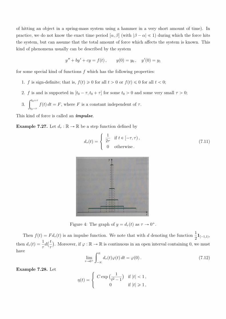
of hitting an object in a spring-mass system using a hammer in a very short amount of time). Inpractice, we do not know the exact time period [α, β] (with |β ´ α| ! 1) during which the force hitsthe system, but can assume that the total amount of force which affects the system is known. Thiskind of phenomena usually can be described by the system

y 11 + by 1 + cy = f(t) , y(0) = y0 , y 1(0) = y1

for some special kind of functions f which has the following properties:

1. f is sign-definite; that is, f(t) ě 0 for all t ą 0 or f(t) ď 0 for all t ă 0;

2. f is and is supported in [t0 ´ τ, t0 + τ ] for some t0 ą 0 and some very small τ ą 0;

3.ż t0+τ

t0´τf(t) dt = F , where F is a constant independent of τ .

This kind of force is called an impulse.

Example 7.27. Let dτ : R Ñ R be a step function defined by

dτ (t) =

$

&

%

1

2τif t P [´τ, τ) ,

0 otherwise .(7.11)

Figure 4: The graph of y = dτ (t) as τ Ñ 0+.

Then f(t) = Fdτ (t) is an impulse function. We note that with d denoting the function 1

21[´1,1),

then dτ (t) =1

τd( tτ

). Moreover, if φ : R Ñ R is continuous in an open interval containing 0, we must

havelimτÑ0+

ż 8

´8

dτ (t)φ(t) dt = φ(0) . (7.12)

Example 7.28. Let

η(t) =

$

&

%

C exp( 1

t2 ´ 1

)if |t| ă 1 ,

0 if |t| ě 1 ,

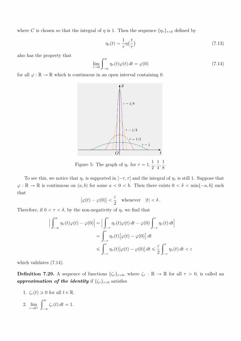
where C is chosen so that the integral of η is 1. Then the sequence tητuτą0 defined by

ητ (t) =1

τη( tτ

)(7.13)

also has the property thatlimτÑ0

ż 8

´8

ητ (t)φ(t) dt = φ(0) (7.14)

for all φ : R Ñ R which is continuous in an open interval containing 0.

Figure 5: The graph of ητ for τ = 1,1

2,1

4,1

8.

To see this, we notice that ητ is supported in [´τ, τ ] and the integral of ητ is still 1. Suppose thatφ : R Ñ R is continuous on (a, b) for some a ă 0 ă b. Then there exists 0 ă δ ă mint´a, bu suchthat

ˇ

ˇφ(t) ´ φ(0)ˇ

ˇ ăε

2whenever |t| ă δ .

Therefore, if 0 ă τ ă δ, by the non-negativity of ητ we find thatˇ

ˇ

ˇ

ż 8

´8

ητ (t)φ(t) ´ φ(0)ˇ

ˇ

ˇ=ˇ

ˇ

ˇ

ż τ

´τ

ητ (t)φ(t) dt ´ φ(0)

ż τ

´τ

ητ (t) dtˇ

ˇ

ˇ

=

ż τ

´τ

ητ (t)[φ(t) ´ φ(0)

]dt

ď

ż τ

´τ

ητ (t)ˇ

ˇφ(t) ´ φ(0)ˇ

ˇ dt ďε

2

ż τ

´τ

ητ (t) dt ă ε

which validates (7.14).

Definition 7.29. A sequence of functions tζτuτą0, where ζτ : R Ñ R for all τ ą 0, is called anapproximation of the identity if tζτuτą0 satisfies

1. ζτ (t) ě 0 for all t P R.

2. limτÑ0+

ż 8

´8

ζτ (t) dt = 1.

3. For all δ ą 0, limτÑ0+

ż

|t|ąδζτ (t) dt = 0.

In particular, tdτuτą0 and tητuτą0 are approximations of identity.

Using the same technique of establishing (7.14), one can also prove that if tζτuτą0 is an approxi-mation of the identity, then

limτÑ0

ż 8

´8

ζτ (t)φ(t) dt = φ(0) .

Remark 7.30. An approximation of identities does not have to be compactly supported. For

example, let n(t) = 1?2πe´ t2

2 be the probability density function of the normal distribution N(0, 1),

then nτ (t) ”1

?2πτ

e´ t2

2τ constitutes an approximation of the identity tnτuτą0.

For t0 ą 0, we consider the ODE

y 11 + by 1 + cy = Fdτ (t ´ t0) , yτ (0) = y0 , y 1τ (0) = y1 . (7.15)

For each 0 ă τ ă t0, let yτ be the solution to (7.15). Using (7.8) we find that

yτ (t) = y8(t) +F

2cτ

[ut0´τ (t)

[1 ´ z(t ´ t0 + τ)

]´ ut0+τ (t)

[1 ´ z(t ´ t0 ´ τ)

]],

where y8 is the unique C 2-function solving

y 118 + by 1

8 + cy8 = 0 , y8(0) = y0 , y 18(0) = y1 .

and z is the unique C 2-function solving

z 11 + bz 1 + cz = 0 , y8(0) = 1 , y 18(0) = 0 .

We remark here that y8, y 18, z 1 and z 11 are of exponential order a for some a P R. We also recall

that the discussion in Section 7.4 shows that yτ is continuously differentiable, and y 11τ is piecewise

continuous. Our “goal” here is to find a function y which is independent of τ but |y ´ yτ | ! 1 whenτ ! 1. In other words, our goal is to show that tyτuτą0 converges and find the limit of tyτuτą0.

We claim that tyτuτą0, viewing as functions defined on [0, T ], is uniformly bounded and equi-continuous (so that we can extract a uniformly convergent subsequence). To see this, using theidentity that

ua+b(t) = ua(t ´ b) (7.16)

we rewrite yτ as

yτ (t) = y8(t) +F

2cτ

[ut0(t+ τ)

[1 ´ z(t ´ t0 + τ)

]´ ut0(t ´ τ)

[1 ´ z(t ´ t0 ´ τ)

]]= y8(t) +

F

2c¨[ut0(t+ τ) ´ ut0(t ´ τ)

][1 ´ z(t ´ t0)

]τ

+F

2c¨ut0(t+ τ)

[z(t ´ t0) ´ z(t ´ t0 + τ)

]τ

´F

2c¨ut0(t ´ τ)

[z(t ´ t0) ´ z(t ´ t0 ´ τ)

]τ

.

By the mean value theorem,

1 ´ z(t ´ t0) = z(0) ´ z(t ´ t0) = (t0 ´ t)z 1(ξ1) for some ξ1 in between 0 and t ´ t0 ,

z(t ´ t0) ´ z(t ´ t0 + τ) = z 1(ξ2)τ for some ξ2 P (t ´ t0, t ´ t0 + τ) ,

z(t ´ t0) ´ z(t ´ t0 ´ τ) = z 1(ξ3)τ for some ξ3 P (t ´ t0 ´ τ, t ´ t0) ;

thus

1. The case ´τ ă t0 ´ t ď τ : in this case we have ut0(t+ τ) ´ ut0(t ´ τ) = 1; thus

|yτ (t)| ď |y8(t)| +ˇ

ˇ

ˇ

F

2c

ˇ

ˇ

ˇ

[|z 1(ξ1)|

|t ´ t0|

τ+ |z 1(ξ2)| + |z 1(ξ3)|

]ď |y8(t)| +

ˇ

ˇ

ˇ

F

2c

ˇ

ˇ

ˇ

[|z 1(ξ1)| + |z 1(ξ2)| + |z 1(ξ3)|

]ď max

tP[0,T ]|y8(t)| +

ˇ

ˇ

ˇ

3F

2c

ˇ

ˇ

ˇmaxtP[0,T ]

|z 1(t)| .

2. The case t0 ´ t R (´τ, τ ]: in this case we have ut0(t+ τ) ´ ut0(t ´ τ) = 0; thus

|yτ (t)| ď |y8(t)| +ˇ

ˇ

ˇ

F

2c

ˇ

ˇ

ˇ

[|z 1(ξ2)| + |z 1(ξ3)|

]ď max

tP[0,T ]|y8(t)| +

ˇ

ˇ

ˇ

F

c

ˇ

ˇ

ˇmaxtP[0,T ]

|z 1(t)| . (7.17)

Therefore, for all τ ą 0 we have

maxtP[0,T ]

|yτ (t)| ď maxtP[0,T ]

|y8(t)| +ˇ

ˇ

ˇ

3F

2c

ˇ

ˇ

ˇmaxtP[0,T ]

|z 1(t)| ď C1eaT

which implies that the sequence tyτ (t)uτą0 is uniformly bounded on [0, T ] and tyτuτą0 are of expo-nential order a.

On the other hand, using (7.9) and (7.16) we have

y 1τ (t) = y 1

8(t) +F

2cτ

[ut0(t ´ τ)z 1(t ´ t0 ´ τ) ´ ut0(t+ τ)z 1(t ´ t0 + τ)

]= y 1

8(t) ´F

2c¨

[ut0(t+ τ) ´ ut0(t ´ τ)

]z 1(t ´ t0)

τ

+F

2c¨ut0(t ´ τ)

[z 1(t ´ t0 ´ τ) ´ z 1(t ´ t0)

]τ

´F

2c¨ut0(t+ τ)

[z 1(t ´ t0 + τ) ´ z 1(t ´ t0)

]τ

.

By the mean value theorem,

z 1(t ´ t0) = z 1(t ´ t0) ´ z 1(0) = z 11(η1)(t ´ t0) for some η1 in between 0 and t ´ t0 ,

z 1(t ´ t0 ´ τ) ´ z 1(t ´ t0) = ´z 1(η2)τ for some η2 in (t ´ t0 ´ τ, t ´ t0) ,

z 1(t ´ t0 + τ) ´ z 1(t ´ t0) = z 1(η3)τ for some η3 in (t ´ t0, t ´ t0 + τ) ,

where we use z 1(0) = 0 to conclude the existence of η1. Similar argument used to conclude thattyτuτą0 is uniformly bounded can then be applied to conclude that

maxtP[0,T ]

|y 1τ (t)

ˇ

ˇ ď maxtP[0,T ]

|y 18(t)| +

ˇ

ˇ

ˇ

3F

2c

ˇ

ˇ

ˇmaxtP[0,T ]

|z 11(t)| ď C2eaT .

This implies that tyτuτą0 is uniformly Lipschitz and are of exponential order a; thus tyτuτą0, viewed asa sequence of functions defined on [0, T ], is equi-continuous. By the Arzelà-Ascoli theorem (Theorem6.42), there exists a subsequence

yτj(8

j=1which converges to y uniformly on [0, T ] as j Ñ 8. We

note that y is a function defined on [0, T ].Now, by the uniform boundedness and equi-continuity of

yτj(8

j=1on [0, T + 1], there exists

a subsequence

yτjℓ(8

ℓ=1which converges to y˚ uniformly on [0, T + 1]. Same procedure provides a

further subsequence

yτjℓk

(8

k=1which converges to y˚˚ uniformly on [0, T + 2]. We note that y˚˚ = y˚

on [0, T + 1] and y˚˚ = y on [0, T ]). We continue this process and obtain a sequence, still denotedby

yτj(8

j=1, and a continuous function y : [0,8) Ñ R such that

yτj(8

j=1converges to y uniformly

on [0, T ] for all T ą 0. We note that (7.17) implies that the limit function y is of exponential ordera for some a ą 0. Moreover, we also note that it is still possible that there is another convergentsubsequence which converges to another limit function, but we will show that there is only onepossible limit function.

Let φ : [0,8) Ñ R be a twice continuously differentiable function which vanishes outside [0, T ]

for some T ą t0. Multiplying the equation above by φ and then integrating on [0, T ], we find thatż T

0

(y 11τj+ by 1

τj+ cyτj

)φ(t) dt = F

ż T

0

dτj(t ´ t0)φ(t) dt .

Integrating by parts (twice if necessary) and making a change of variable on the right-hand side,

y0φ1(0) ´

(y1 + by0

)φ(0) +

ż 8

0

yτj(t)(φ 11(t) ´ bφ 1(t) + cφ(t)

)dt = F

ż 8

´8

dτj(t)φ(t+ t0) dt (7.18)

for all twice continuously differentiable functions φ vanishing outside some interval [0, T ]. We notethat the integral in (7.18) is not an improper integral but indeed an integral on a bounded interval.Passing to the limit as j Ñ 8 in (7.18), the uniform convergence of

yτj(8

j=1to y on any closed

interval [0, T ] and (7.12) imply that

y0φ1(0) ´

(y1 + by0

)φ(0) +

ż 8

0

y(t)(φ 11(t) ´ bφ 1(t) + cφ(t)

)dt = Fφ(t0) (7.19)

for all twice continuously differentiable functions φ vanishing outside some interval [0, T ]. Since y isof exponential order a, (7.19) in fact holds for all twice continuously differentiable function φ whichapproaches 0 fast enough at infinity, here the sentence “φ approaches 0 fast enough at infinity” meansthat

ˇ

ˇφ(t)ˇ

ˇ+ˇ

ˇφ 1(t)ˇ

ˇ+ˇ

ˇφ 11(t)ˇ

ˇ ď Me´rat @ t " 1

for some ra ą a.To see what a possible limit function y is, we let φ(t) = e´st for s ą a in (7.19) and obtain that

´sy0 ´ (y1 + by0) + (s2 + bs+ c)

ż 8

0

y(t)e´st dt = Fe´st0

which, by the definition of the Laplace transform, implies that

(s2 + bs+ c)L (y)(s) = (s+ b)y0 + y1 + Fe´st0 . (7.20)

Since every possible limit y of tyτuτą0 is continuous and is of exponential order a, by Theorem 7.10we conclude that there is only one uniform limit of tyτuτą0; thus tyτuτą0 converges to y uniformlyon [0, T ] for every T ą 0. By Theorem 7.19 and 7.22, identity (7.20) implies the following:

1. if r2 + br + c = 0 has two distinct real roots r1 and r2, then the solution y to (7.20) is

y(t) = y8(t) +F

r1 ´ r2ut0(t)

[er1(t´t0) ´ er2(t´t0)

]=y1 ´ r2y0r1 ´ r2

er1t +r1y0 ´ y1r1 ´ r2

er2t +F

r1 ´ r2ut0(t)

[er1(t´t0) ´ er2(t´t0)

]. (7.21)

2. if r2 + br + c = 0 has a double root r1, then the solution y to (7.20) is

y(t) = y8(t) + Fut0(t)(t ´ t0)er1(t´t0)

= y0er1t + (y1 ´ r1y0)te

r1t + Fut0(t)(t ´ t0)er1(t´t0) . (7.22)

3. if r2 + br + c = 0 has two complex roots λ ˘ iµ, then the solution y to (7.20) is

y(t) = y8(t) +F

µut0(t)e

λ(t´t0) sinµ(t ´ t0)

= y0eλt cosµt+ y1 ´ λy0

µeλt sinµt+ F

µut0(t)e

λ(t´t0) sinµ(t ´ t0) . (7.23)

The uniform convergence of tyτuτą0 to y implies that if the support of the impulse is really small,even though we might not know the precise value of τ , the solution to (7.15) is very closed to theunique limit function y. We note that the three possible y’s given above are continuous but havediscontinuous derivatives, and are not differentiable at t0.

7.5.1 The Dirac delta function

Even though we can stop our discussion about second order ODEs with impulse forcing functionshere, we would like to go a little bit further by introducing the so-called “Dirac delta function”.Taking (7.3) into account, (7.20) motivates the following

Definition 7.31 (Informal definition of the Dirac delta function). For t0 ą 0, the Dirac deltafunction at t0, denoted by δt0 , is the function whose Laplace transform is the function G(s) = e´st0 .

Therefore, (7.3) and (7.20) imply that y satisfies the ODE

y 11 + by 1 + cy = Fδt0(t) , y(0) = y0, y 1(0) = y1 . (7.24)

By Theorem 7.19, in order to obtain the precise form of δt0 it suffices to find the function whoseLaplace transform is the constant 1. However, this δt0 is not a function of non-negative real numberssince we actually have

y 11(t) + by 1(t) + cy(t) = 0 @ t ‰ t0

if y is given by (7.21), (7.22) or (7.22). If δt0 is a function of non-negative real numbers, no matterwhat value is assigned to δt0(t0), the Laplace transform of δt0 cannot be constant 1.

‚ What does y 11+by 1+cy = Fδt0(t) really mean? Recall that our goal is to find a “representative”of solutions of the sequence of ODEs (7.15). The discussion above shows that such a representativehas to satisfies (7.20) which, under the assumption that

L (y 11 + by 1 + cy)(s) = (s2 + bs+ c)L (y) ´ sy(0) ´ y 1(0) . (7.25)

implies the equation y 11 + by 1 + cy = Fδt0(t). As we can see from the precise form of the function y

in (7.21), (7.22) and (7.23), y 1 is not even continuous; thus (7.25) is in fact a false assumption.The way that the ODE y 11 + by 1 + cy = Fδt0(t) is understood is through the distribution theory,

in which both sides of the ODE are treated as “functions of functions”. Before our discussion, let usfirst have the following two definitions.

Definition 7.32. The collection of all k-times continuously differentiable function defined on [0,8

and vanishing outside some interval [0, T ] for some T ą 0 is denoted by C kc ([0,8)). A function

f : [0,8) Ñ R is said to belong to the space C 8c ([0,8)) if f P C k

c ([0,8)) for all k P N. In otherwords,

C 8c ([0,8)) ”

!

f : [0,8) Ñ Rˇ

ˇ

ˇf P C k

c ([0,8) @ k P N)

.

Definition 7.33. Let f : [0,8) be a piecewise continuous function. The linear functional inducedby f , denoted by xf, ¨y, is a function on C 8

c ([0,8)) given by

xf, φy =

ż 8

0

f(t)φ(t) dt @φ P C 8c ([0,8)) .

Consider the following simple ODE

y 11 + by 1 + cy = f(t) , y(0) = y0 , y 1(0) = y1 , (7.26)

where f is a continuous function of exponential order a for some a P R. The existence theoryimplies that there exists a unique twice continuously differentiable solution y to (7.26). Moreover, ifφ P C 2

c ([0,8)),ż 8

0

[y 11(t) + by 1(t) + cy(t)

]φ(t) dt =

ż 8

0

f(t)φ(t) dt , y(0) = y0 , y1(0) = y1 . (7.27)

Since y is twice continuously differentiable on [0,8), we can integrate by parts and find that thesolution y to (7.26) also satisfies

y0φ1(0) ´

(y1 + by0

)φ(0) +

ż 8

0

y(t)(φ 11(t) ´ bφ 1(t) + cφ(t)

)dt = xf, φy @φ P C 2

c ([0,8)) . (7.28)

On the other hand, if y is a twice continuously differentiable function satisfying (7.28), we canintegrate by parts (to put the derivatives on φ back to y) and find that y satisfies(

y0 ´ y(0))φ 1(0) ´

[y1 + by0 ´ y 1(0) ´ by(0)

]φ(0)

+

ż 8

0

[y 11(t) + by 1(t) + cy(t)

]φ(t) dt =

ż 8

0

f(t)φ(t) dt@φ P C 2

c ([0,8)) .

In particular,ż 8

0

[y 11(t) + by 1(t) + cy(t)

]φ(t) dt =

ż 8

0

f(t)φ(t) dt @φ P C 2c ([0,8)) satisfying φ(0) = φ 1(0) = 0 .

Therefore, y 11 + by 1 + cy must be identical to f since they are both continuous. Having establishedthis, we find that(

y0 ´ y(0))φ 1(0) ´

[y1 + by0 ´ y 1(0) ´ by(0)

]φ(0) = 0 @φ P C 2

c ([0,8)) .

Choose φ P C 2c ([0,8)) such that φ(0) = 0 and φ 1(0) = 1, we conclude that y0 = y(0); thus we arrive

at the equality [y1 + by0 ´ y 1(0) ´ by(0)

]φ(0) = 0 @φ P C 2

c ([0,8)) .

The identity above clearly shows that y1 = y 1(0). In other words, if y is twice continuously differen-tiable and satisfies (7.28), then y satisfies (7.26); thus we establish that given a continuous forcingfunction f ,

y is a solution to (7.26) if and only if y satisfies (7.28).

Thus we change the problem of solving an ODE “in the pointwise sense” to a problem of solvingan integral equation which holds “in the sense of distribution” (a distribution means a function offunctions). We note that there is one particular advantage of defining solution to (7.26) using (7.28)instead of (7.27): if f is discontinuous somewhere in [0,8) (for example, f = F1[α,β) as in theprevious section), (7.28) provides a good alternative even if y 11 does not always exist.

The discussion above motivates the following

Definition 7.34 (Weak Solutions). Let f : [0,8) Ñ R be a function of exponential order a for somea P R. A function y : [0,8) Ñ R is said to be a weak solution to (7.26) if y satisfies the integralequation (7.28). The integral equation (7.28) is called the weak formulation of (7.26).

We remark that the discussion above shows that if f : [0,8) Ñ R is continuous and of exponentialorder a for some a P R, the unique C 2-solution y to (7.26) is also a weak solution.

In view of (7.28), if we define L : C 2c ([0,8)) Ñ R by

L(φ) = y0φ1(0) ´

(y1 + by0

)φ(0) +

ż 8

0

y(t)(φ 11(t) ´ bφ 1(t) + cφ(t)

)dt , (7.29)

then the integral equation (7.26) is equivalent to that “the two linear functionals L and xf, ¨y are thesame on the space C 2

c ([0,8))”. We also note that

L(φ) = xy 11 + by 1 + cy, φy if y 11 is piecewise continuous, and (y(0), y 1(0)) = (y0, y1) ;

thus if y 11 is piecewise continuous, the statement “L = xf, ¨y on C 2c ([0,8))” is the same as saying that

“the linear functional induced by y 11 + by 1 + cy and the linear functional induced by f are identical”.This is what it means by y 11 + by 1 + cy = f in the sense of distribution.

If the right-hand side xf, ¨y is replaced by a general linear functional ℓ, we can still talk aboutthe possibility of finding an integrable function y validating the integral equation (7.28), or more

precisely, L = ℓ on C 2c ([0,8)). In particular, for F P R and t0 ą 0, it is reasonable to ask whether

or not there exists an integrable function y such that

y0φ1(0) ´

(y1 + by0

)φ(0) +

ż 8

0

y(t)(φ 11(t) ´ bφ 1(t) + cφ(t)

)dt = Fφ(t0) @φ P C 2

c ([0,8)) , (7.19)

where the linear functional ℓ : C 2c ([0,8)) Ñ R is given by

ℓ(φ) = Fφ(t0) @φ P C 2c ([0,8)) . (7.30)

This is exactly the integral equation (7.19); thus the ODE y 11 + by 1 + cy = Fδt0(t) is understood asL = ℓ on C 2

c ([0,8)), where L and ℓ are defined by (7.29) and (7.30), respectively.The definition of ℓ motivates the following

Definition 7.35 (Dirac Delta Function). For t0 P R, let X (t0) denote the collection of functionsdefined on R and continuous on an open interval containing t0. The Dirac delta function at t0 isa map δt0 : X (t0) Ñ R defined by

δt0(φ) = φ(t0) .

The map δ0 is usually denoted as δ.

Under this definition, the ODE y 11 + by 1 + cy = Fδt0 is understood as “the functional induced byy 11 + by 1 + cy (given by (7.29)) is the same as the functional induced by Fδt0”. The function y givenby (7.21), (7.22) or (7.23) is then a weak solution to (7.24).

Example 7.36. In this example, we would like to find the “anti-derivative” of the Dirac deltafunction at t0 ą 0. In other words, we are looking for a solution to

y 1 = δt0(t) , y(0) = 0 , y 1(0) = 0 .

Taking the Laplace transform, we find that

sL (y)(s) = e´st0 or equivalently, L (y)(s) =e´st0

s. (7.31)

As a consequence, by Example 7.5 and Theorem 7.19 we conclude that the (weak) solution to theODE above is

y(t) = ut0(t) = H(t ´ t0) .

We again emphasize that in principle we are not allowed to use Theorem 7.12 or Corollary 7.13 tocompute the Laplace transform of y 1; however, the functional induced by y 1 (by assuming that y is

ż 8

0

y 1(t)φ(t) dt = y(0)φ(0) ´

ż 8

0

y(t)φ 1(t) dt

so we are in fact solving y 1 = δt0(t) in the sense of distribution; that is, we look for y satisfying

´

ż 8

0

y(t)φ 1(t) dt = φ(t0) @φ P X.

Letting φ(t) = e´st leads to (7.31).

7.6 The Convolution Integrals

Definition 7.37. Let f, g be piecewise continuous on [0,8). The convolution of f and g, denotedby f ˙ g, is defined by

(f ˙ g)(t) =

ż t

0

f(t ´ τ)g(τ) dτ . (7.32)

Proposition 7.38. Let f, g, h be piecewise continuous on [0,8). Then

(a) f ˙ g = g ˙ f ;

(b) f ˙ (g + h) = (f ˙ g) + (f ˙ h);

(c) (f ˙ g) ˙ h = f ˙ (g ˙ h);

(d) (f ˙ 0) = 0.

Theorem 7.39. Let f and g be piecewise continuous on [0,8) and are of exponential order a. Then

L (f ˙ g)(s) = L (f)(s)L (g)(s) @ s ą a .

Proof. Since f is of exponential order a, for some M1 ą 0, |f(t)| ď M1eat for all t ą 0. Therefore,

for s ą a,ˇ

ˇ

ˇL (f)(s) ´

ż R

0

e´stf(t) dtˇ

ˇ

ˇď

ż 8

R

e´stˇ

ˇf(t)ˇ

ˇ dt ď M1

ż 8

R

e´(s´a)tdt ďM1

s ´ ae(a´s)R .

Similarly, for some M2 ą 0, |g(t)| ď M2eat for all t ą 0 and

ˇ

ˇ

ˇL (g)(s) ´

ż R

0e´stg(t) dt

ˇ

ˇ

ˇď

M2

s ´ ae(a´s)R @ s ą a .

By the Fubini theorem,ż R

0

e´st( ż t

0

f(t ´ τ)g(τ) dτ)dt =

ż R

0

( ż R

τ

f(t ´ τ)g(τ)e´st dt)dτ

=

ż R

0

e´sτg(τ)( ż R

τ

f(t ´ τ)e´s(t´τ) dt)dτ =

ż R

0

e´sτg(τ)( ż R´τ

0

f(t)e´st dt)dτ ;

thus for s ą a,ˇ

ˇ

ˇ

ż R

0

e´st( ż t

0

f(t ´ τ)g(τ) dτ)dt ´ L (f)(s)L (g)(s)

ˇ

ˇ

ˇ

=ˇ

ˇ

ˇ

ż R

0

e´sτg(τ)( ż R´τ

0

f(t)e´st dt)dτ ´ L (f)(s)L (g)(s)

ˇ

ˇ

ˇ

=ˇ

ˇ

ˇ

ż R

0

e´sτg(τ)( ż R´τ

0

f(t)e´st dt ´ L (f)(s))dτ + L (f)(s)

( ż R

0

e´sτg(τ) dτ ´ L (g)(s))ˇˇ

ˇ

ďM1M2

s ´ a

ż R

0

e´sτeaτe(a´s)(R´τ) dτ +M2

s ´ a

ˇ

ˇL (f)(s)ˇ

ˇe(a´s)R

=M1M2

s ´ aRe(a´s)R +

M2

s ´ a

ˇ

ˇL (f)(s)ˇ

ˇe(a´s)R

which converges to 0 as R Ñ 8. ˝

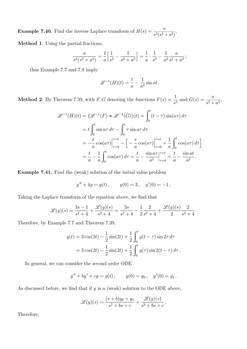
Example 7.40. Find the inverse Laplace transform of H(s) =a

s2(s2 + a2).

Method 1: Using the partial fractions,

a

s2(s2 + a2)=

1

a

[ 1

s2´

1

s2 + a2

]=

1

a¨1

s2´

1

a2a

s2 + a2;

thus Example 7.7 and 7.9 imply

L ´1(H)(t) =t

a´

1

a2sin at .

Method 2: By Theorem 7.39, with F,G denoting the functions F (s) = 1

s2and G(s) =

a

s2 + a2,

L ´1(H)(t) =(L ´1(F ) ˙ L ´1(G)

)(t) =

ż t

0

(t ´ τ) sin(aτ) dτ

= t

ż t

0

sin aτ dτ ´

ż t

0

τ sin aτ dτ

= ´t

acos(aτ)

ˇ

ˇ

ˇ

τ=t

τ=0´

[´τ

acos(aτ)

ˇ

ˇ

ˇ

τ=t

τ=0+

1

a

ż t

0

cos(aτ) dτ]

=t

a´

1

a

ż t

0

cos(aτ) dτ =t

a´

sin aτa2

ˇ

ˇ

ˇ

τ=t

τ=0=t

a´

sin ata2

.

Example 7.41. Find the (weak) solution of the initial value problem

y 11 + 4y = g(t) , y(0) = 3 , y 1(0) = ´1 .

Taking the Laplace transform of the equation above, we find that

L (y)(s) =3s ´ 1

s2 + 4+

L (g)(s)

s2 + 4=

3s

s2 + 4´

1

2

2

s2 + 4+

L (g)(s)

2

2

s2 + 4.

Therefore, by Example 7.7 and Theorem 7.39,

y(t) = 3 cos(2t) ´1

2sin(2t) + 1

2

ż t

0

g(t ´ τ) sin 2τ dτ

= 3 cos(2t) ´1

2sin(2t) + 1

2

ż t

0

g(τ) sin 2(t ´ τ) dτ .

In general, we can consider the second order ODE

y 11 + by 1 + cy = g(t) , y(0) = y0 , y 1(0) = y1 .

As discussed before, we find that if y is a (weak) solution to the ODE above,

L (y)(s) =(s+ b)y0 + y1s2 + bs+ c

+L (g)(s)

s2 + bs+ c.

Therefore,

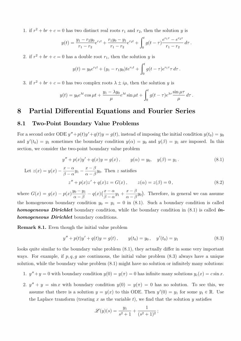
1. if r2 + br + c = 0 has two distinct real roots r1 and r2, then the solution y is

y(t) =y1 ´ r2y0r1 ´ r2

er1t +r1y0 ´ y1r1 ´ r2

er2t +

ż t

0

g(t ´ τ)er1τ ´ er2τ

r1 ´ r2dτ .

2. if r2 + br + c = 0 has a double root r1, then the solution y is

y(t) = y0er1t + (y1 ´ r1y0)te

r1t +

ż t

0

g(t ´ τ)er1ττ dτ .

3. if r2 + br + c = 0 has two complex roots λ ˘ iµ, then the solution y is

y(t) = y0eλt cosµt+ y1 ´ λy0

µeλt sinµt+

ż t

0

g(t ´ τ)eλτsinµτµ

dτ .

8 Partial Differential Equations and Fourier Series

8.1 Two-Point Boundary Value Problems

For a second order ODE y 11+p(t)y 1+q(t)y = g(t), instead of imposing the initial condition y(t0) = y0

and y 1(t0) = y1 sometimes the boundary condition y(α) = y0 and y(β) = y1 are imposed. In thissection, we consider the two-point boundary value problem

y 11 + p(x)y 1 + q(x)y = g(x) , y(α) = y0, y(β) = y1 . (8.1)

Let z(x) = y(x) ´x ´ α

β ´ αy1 ´

x ´ β

α ´ βy0. Then z satisfies

z 11 + p(x)z 1 + q(x)z = G(x) , z(α) = z(β) = 0 , (8.2)

where G(x) = g(x) ´ p(x)y0 ´ y1α ´ β

´ q(x)(x ´ α

β ´ αy1 +

x ´ β

α ´ βy0). Therefore, in general we can assume

the homogeneous boundary condition y0 = y1 = 0 in (8.1). Such a boundary condition is calledhomogeneous Dirichlet boundary condition, while the boundary condition in (8.1) is called in-homogeneous Dirichlet boundary conditions.

Remark 8.1. Even though the initial value problem

y 11 + p(t)y 1 + q(t)y = g(t) , y(t0) = y0 , y 1(t0) = y1 (8.3)

looks quite similar to the boundary value problem (8.1), they actually differ in some very importantways. For example, if p, q, g are continuous, the initial value problem (8.3) always have a uniquesolution, while the boundary value problem (8.1) might have no solution or infinitely many solutions:

1. y 11+y = 0 with boundary condition y(0) = y(π) = 0 has infinite many solutions yc(x) = c sinx.

2. y 11 + y = sinx with boundary condition y(0) = y(π) = 0 has no solution. To see this, weassume that there is a solution y = y(x) to this ODE. Then y 1(0) = y1 for some y1 P R. Usethe Laplace transform (treating x as the variable t), we find that the solution y satisfies

L (y)(s) =y1

s2 + 1+

1

(s2 + 1)2;

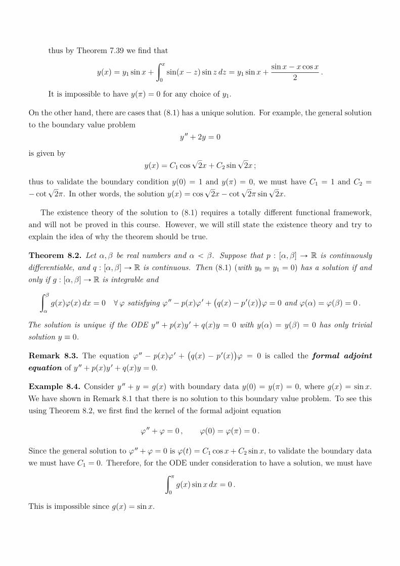
thus by Theorem 7.39 we find that

y(x) = y1 sinx+ż x

0

sin(x ´ z) sin z dz = y1 sinx+ sin x ´ x cosx2

.

It is impossible to have y(π) = 0 for any choice of y1.

On the other hand, there are cases that (8.1) has a unique solution. For example, the general solutionto the boundary value problem

y 11 + 2y = 0

is given byy(x) = C1 cos

?2x+ C2 sin

?2x ;

thus to validate the boundary condition y(0) = 1 and y(π) = 0, we must have C1 = 1 and C2 =

´ cot?2π. In other words, the solution y(x) = cos

?2x ´ cot

?2π sin

?2x.

The existence theory of the solution to (8.1) requires a totally different functional framework,and will not be proved in this course. However, we will still state the existence theory and try toexplain the idea of why the theorem should be true.

Theorem 8.2. Let α, β be real numbers and α ă β. Suppose that p : [α, β] Ñ R is continuouslydifferentiable, and q : [α, β] Ñ R is continuous. Then (8.1) (with y0 = y1 = 0) has a solution if andonly if g : [α, β] Ñ R is integrable and

ż β

α

g(x)φ(x) dx = 0 @φ satisfying φ 11 ´ p(x)φ 1 +(q(x) ´ p 1(x)

)φ = 0 and φ(α) = φ(β) = 0 .

The solution is unique if the ODE y 11 + p(x)y 1 + q(x)y = 0 with y(α) = y(β) = 0 has only trivialsolution y ” 0.

Remark 8.3. The equation φ 11 ´ p(x)φ 1 +(q(x) ´ p 1(x)

)φ = 0 is called the formal adjoint

equation of y 11 + p(x)y 1 + q(x)y = 0.

Example 8.4. Consider y 11 + y = g(x) with boundary data y(0) = y(π) = 0, where g(x) = sinx.We have shown in Remark 8.1 that there is no solution to this boundary value problem. To see thisusing Theorem 8.2, we first find the kernel of the formal adjoint equation

φ 11 + φ = 0 , φ(0) = φ(π) = 0 .

Since the general solution to φ 11 + φ = 0 is φ(t) = C1 cosx+C2 sinx, to validate the boundary datawe must have C1 = 0. Therefore, for the ODE under consideration to have a solution, we must have

ż π

0

g(x) sinx dx = 0 .

This is impossible since g(x) = sinx.

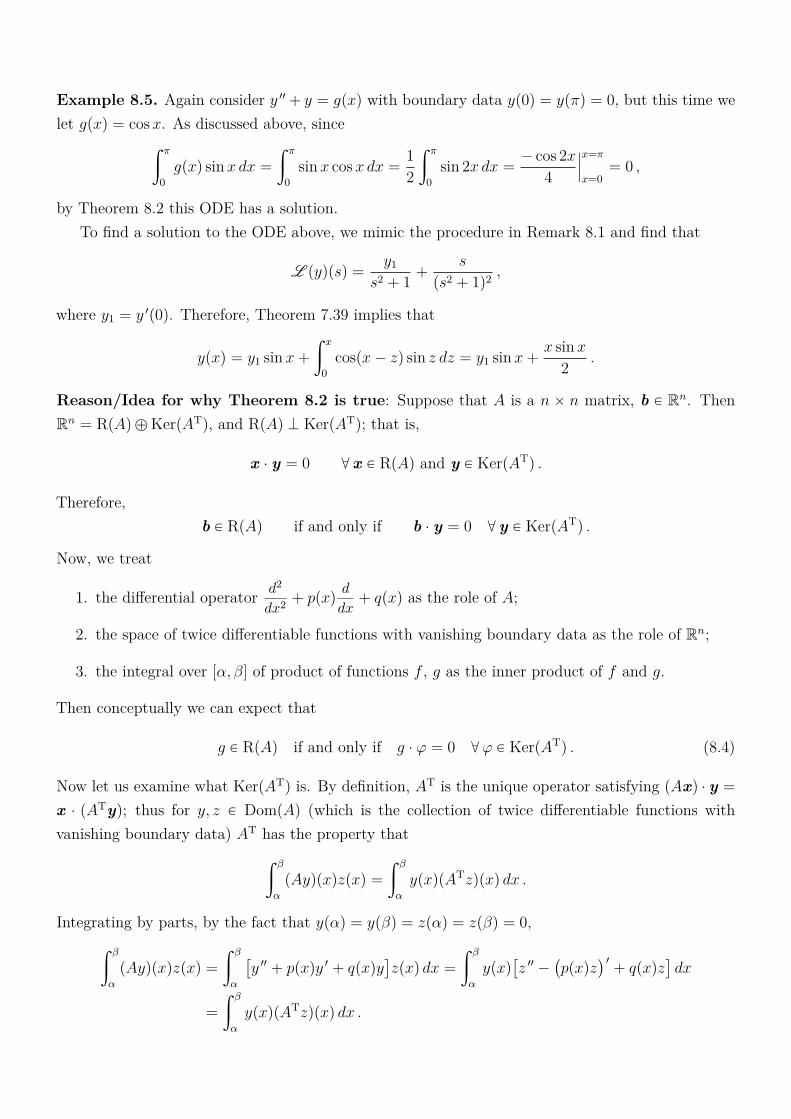
Example 8.5. Again consider y 11 + y = g(x) with boundary data y(0) = y(π) = 0, but this time welet g(x) = cosx. As discussed above, since

ż π

0

g(x) sinx dx =

ż π

0

sinx cos x dx =1

2

ż π

0

sin 2x dx =´ cos 2x

4

ˇ

ˇ

ˇ

x=π

x=0= 0 ,

by Theorem 8.2 this ODE has a solution.To find a solution to the ODE above, we mimic the procedure in Remark 8.1 and find that

L (y)(s) =y1

s2 + 1+

s

(s2 + 1)2,

where y1 = y 1(0). Therefore, Theorem 7.39 implies that

y(x) = y1 sinx+ż x

0

cos(x ´ z) sin z dz = y1 sinx+ x sin x2

.

Reason/Idea for why Theorem 8.2 is true: Suppose that A is a n ˆ n matrix, b P Rn. ThenRn = R(A) ‘ Ker(AT), and R(A) K Ker(AT); that is,

x ¨ y = 0 @ x P R(A) and y P Ker(AT) .

Therefore,b P R(A) if and only if b ¨ y = 0 @ y P Ker(AT) .

Now, we treat

1. the differential operator d2

dx2+ p(x)

d

dx+ q(x) as the role of A;

2. the space of twice differentiable functions with vanishing boundary data as the role of Rn;

3. the integral over [α, β] of product of functions f , g as the inner product of f and g.

Then conceptually we can expect that

g P R(A) if and only if g ¨ φ = 0 @φ P Ker(AT) . (8.4)

Now let us examine what Ker(AT) is. By definition, AT is the unique operator satisfying (Ax) ¨ y =

x ¨ (ATy); thus for y, z P Dom(A) (which is the collection of twice differentiable functions withvanishing boundary data) AT has the property that

ż β

α

(Ay)(x)z(x) =

ż β

α

y(x)(ATz)(x) dx .

Integrating by parts, by the fact that y(α) = y(β) = z(α) = z(β) = 0,ż β

α

(Ay)(x)z(x) =

ż β

α

[y 11 + p(x)y 1 + q(x)y

]z(x) dx =

ż β

α

y(x)[z 11 ´

(p(x)z

) 1+ q(x)z

]dx

=

ż β

α

y(x)(ATz)(x) dx .

Therefore, AT is the differential operator d2

dx2´ p(x)

d

dx+(q(x) ´ p 1(x)

). Note that g P R(A) means

D y P Dom(A) Q y 11 + p(x)y 1 + q(x)y = g(x) ;

thus (8.4) implies that

D y P Dom(A) Q y 11 + p(x)y 1 + q(x)y = g(x)

ô

ż β

α

g(x)φ(x) dx = 0 @φ satisfying φ 11 ´ p(x)φ 1 +(q(x) ´ p 1(x)

)φ = 0 .

This is exactly what Theorem 8.2 is talking about. However, we emphasize that the argument aboveis purely conceptually but not rigorous.

8.1.1 Eigenfunctions

Recall that if A is a real symmetric n ˆ n matrix, then it is diagonalizable and there exists anorthonormal basis of Rn consisting of eigenvectors of A. Similarly, if a second order differentialoperator

A =d2

dx2+ p(x)

d

dx+ q(x) (8.5)

is self-adjoint (meaning A = AT, where AT is given by ATφ = φ 11 ´ p(x)φ 1 + (q(x) ´ p 1(x))φ),then the eigenvectors of A, called the eigenfunctions of A, can also form an orthonormal basis ofDom(A). We note that for a differential operator A given by (8.5) being self-adjoint, it is sufficientand necessary that p ” 0. In particular, we consider the eigenfunctions u of the differential operator

∆ =d2

dx2satisfying

∆u = u 11 = λu , u(α) = u(β) = 0 (α ă β) . (8.6)

If λ ą 0, then the general solution to (8.6) is u(x) = C1e?λx + C2e

´?λx which, to validate the

boundary data, implies that C1 = C2 = 0. Therefore, the eigenvalue of the differential operator ∆

cannot be positive.If λ ď 0, the general solution to (8.6) is u(x) = C1 cos

?´λx + C2 sin

?´λx. To satisfy the

boundary data, it is required that[cos

?´λα sin

?´λα

cos?

´λβ sin?

´λβ

] [C1

C2

]=

[00

]Since we are interested in the case that C1 or C2 ‰ 0, we must have

det([

cos?

´λα sin?

´λαcos

?´λβ sin

?´λβ

])= 0 ;

thus sin?

´λ(β ´ α) = 0. This implies that?

´λ(β ´ α) = kπ or some k; thus λ = ´k2π2

(β ´ α)2. A

corresponding eigenfunction is then

u(x) = ´ sin kπα

β ´ αcos kπx

β ´ α+ cos kπα

β ´ αsin kπx

β ´ α= sin kπ(x ´ α)

β ´ α.

For each k P N, define

λk = ´k2π2

(β ´ α)2and ek(x) =

c

2

β ´ αsin kπ(x ´ α)

β ´ α, (8.7)

where the constantc

2

β ´ αis for the purpose that teku8

k=1 forms an orthonormal set; that is, we

have the property that ek ¨ ej = δkj, or to be more precisely,ż β

α

ek(x)ej(x) dx =

"

1 if k = j ,0 if k ‰ j .

Then we expect that for twice differentiable function φ with vanishing Dirichlet boundary data,

φ(x) =8ÿ

k=1

(φ ¨ ek)ek(x) =8ÿ

k=1

ż β

α

φ(y)ek(y) dy ek(x) @x P [α, β] (8.8)

and the “length” of the function φ should obey the Pythagorean Theorem; that is, one expects thatż β

α

φ(x)2 dx =8ÿ

k=1

( ż β

α

φ(y)ek(y) dy)2

(8.9)

Identity (8.8), often called the Fourier series representation (for functions vanishing on theboundary), in fact holds for all φ which satisfies φ(α) = φ(β) and is Hölder continuous with someHölder exponent; that is, there is α P (0, 1] such that

supx1,x2P[α,β]

ˇ

ˇφ(x1) ´ φ(x2)ˇ

ˇ

|x1 ´ x2|αă 8 ,

while (8.9), called the Parseval identity, even holds for a larger class of functions. We againemphasize that the derivation of (8.8) is not rigorous but purely conceptually.

Instead of considering the second order equation y 11 +p(t)y 1 + q(t)y = g(t) with boundary y(α) =y(β) = 0, we can also consider the following three type of boundary conditions:

1. y 1(α) = a, y 1(β) = b, called the inhomogeneous Neumann boundary condition, or

2. y(α) = 0, y 1(β) = b or y 1(α) = a, y 1(β) = 0, called the mixed type boundary condition.

We note that in either cases, using similar technique to transform (8.1) to (8.2) we can alwaystransform the boundary condition above to the homogeneous one; that is,

1. y 1(α) = 0, y 1(β) = 0, called the homogeneous Neumann boundary condition, or

2. y(α) = 0, y 1(β) = 0 or y 1(α) = 0, y 1(β) = 0.

Now we consider the eigenfunctions for the differential operator ∆ with different boundary conditions.

1. Homogeneous Neumann boundary conditions: We look for u : [α, β] Ñ R satisfying

uxx = λu in [α, β], u 1(α) = u 1(β) = 0 .

As in the previous section, if λ ą 0, then the only possible u is trivial, so we consider the caseλ ď 0. If λ = 0, we have u(x) = 1 being a non-trivial eigenfunction. If λ ă 0, the generalsolution to the ODE (without specifying the boundary condition) is

u(x) = C1 cos?

´λx+ C2 sin?

´λx ,

and to validate the boundary condition, the system[´ sin

?´λα cos

?´λα

´ sin?

´λβ cos?

´λβ

] [C1

C2

]=

[00

]must have non-trivial solution which implies sin

?´λ(β ´ α) = 0. As in the previous section,

we conclude that

λ = ´k2π2

(β ´ α)2and u(x) = C cos

?´λ(x ´ α) = C cos kπ(x ´ α)

β ´ α.

For each k P N, define

λk = ´k2π2

(β ´ α)2, e0(x) =

c

1

β ´ αand ek(x) =

c

2

β ´ αcos kπ(x ´ α)

β ´ α. (8.10)

Then teku8k=0 forms an orthonormal “basis” in the space

u P C 2([α, β])ˇ

ˇu 1(α) = u 1(β) = 0(

;

that is, for twice differentiable function φ with vanishing Neumann boundary data,

φ(x) =8ÿ

k=0

(φ ¨ ek)ek(x) =8ÿ

k=1

ż β

α

φ(y)ek(y) dy ek(x) @x P (α, β) (8.11)

and the “length” of the function φ should obey the Parseval identityż β

α

φ(x)2 dx =8ÿ

k=1

( ż β

α

φ(y)ek(y) dy)2

(8.12)

2. Mixed type boundary conditions: We first look for u : [α, β] Ñ R satisfying

uxx = λu in [α, β], u(α) = u 1(β) = 0 .

Similar computations show that λ ă 0 and cos?

´λ(α ´ β) = 0. Therefore,?

´λ(β ´ α) =(2k + 1)π

2which implies that for some k P N,

λ = ´(2k ´ 1)2π2

4(β ´ α)2.

Therefore, for each k P N, define

λk = ´(2k ´ 1)2π2

4(β ´ α)2and ek(x) =

c

2

β ´ αsin (2k ´ 1)π(x ´ α)

2(β ´ α).

Then teku8k=1 forms an orthonormal “basis” in the space

u P C 2([α, β])ˇ

ˇu(α) = u 1(β) = 0(

.

Similarly,!

c

2

β ´ αcos (2k ´ 1)π(x ´ α)

2(β ´ α)

)8

k=1forms an orthonormal “basis” in the space

u P

C 2([α, β])ˇ

ˇu 1(α) = u(β) = 0(

.

8.2 Fourier Series

In the previous section, we discuss how one obtain an orthonormal basis in different spaces. In fact,by the Stone-Weierstrass Theorem (abstract version) we can conclude the following

Theorem 8.6. Let C (T) be the collection of all 2π-periodic continuous functions, and Pn(T) be thecollection of all trigonometric polynomials of degree n; that is,

Pn(T) =!

c02+

nÿ

k=1

ck cos kx+ sk sin kxˇ

ˇ

ˇtckunk=0, tskunk=1 Ď R

)

.

Let P(T) =8Ť

n=0

Pn(T). Then P(T) is dense in C (T). In other words, if f P C (T) and ε ą 0 is

given, there exists p P P(T) such thatˇ

ˇf(x) ´ p(x)ˇ

ˇ ă ε @ x P R .

In other words, every period function with period 2π can be approximated by trigonometricpolynomials in the uniform sense. In this section, we would like to discuss how to approximate acontinuous period functions using trigonometric polynomials.

背景知識：Stone-Weierstrass 定理（concrete version）告訴我們定義在 [0, 1] 上的連續函數 f 可以

用多項式（例如 Bernstein 多項式）去逼近（在均勻收斂的意義下），而我們也注意到 Bernstein 多項式，在取不同次數 n 的多項式做逼近時，每一個單項式 xk 前面的係數都跟 n 和 k 有關。但是

從 Taylor 定理中我們又發現，對某些擁有很好性質的函數 f（叫做解析函數 Analytic functions），即使取不同次數 n 的多項式做逼近時，每個單項式 xk 前面的係數可以取成只跟函數 f 的 k 次導

數有關（跟 n 無關）。這給了我們一個很粗略的概念，知道想用多項式去逼近連續函數時，多項式

的係數有些時候會跟多項次的次數有關，有時則無關。

在這一節中，我們特別關注連續的週期函數。由 Theorem 8.6 我們知道週期為 2π 的函數可用

形如

pn(x) =c(n)0

2+

nÿ

k=1

(c(n)k cos kx+ s

(n)k sin kx)

的三角多項式 (trigonometric polynomials) 所逼近（在均勻收斂的意義下），其中上標 (n) 代表的

是係數可能與用來逼近的三角多項式的次數 n 有關係。跟前一段所述的經驗類似，在數學理論上

我們想知道下面問題的答案：

1. 什麼樣的函數，可以用係數與逼近次數無關的三角多項式去逼近。對這樣的函數，三角多項式要怎麼挑？

2. 對於實在沒辦法用係數與逼近次數無關的三角多項式去逼近的連續週期函數，有什麼好的方法逼近？而上面所挑出來的那個係數跟逼近次數無關的三角多項式，在次數接近無窮大時出

了什麼問題？

Let f P C (T) be given. We first assume that the trigonometric polynomials used to approximatef can be chosen in such a way that the coefficients does not depend on the degree of approximation;

that is, c(n)k = ck and s(n)k = sk. In this case, if pn Ñ f uniformy on [´π, π], we must have

limnÑ8

ż π

´π

pn(x) cos kx dx =

ż π

´π

f(x) cos kx dx @ k P t0, 1, ¨ ¨ ¨ , nu

andlimnÑ8

ż π

´π

pn(x) sin kx dx =

ż π

´π

f(x) sin kx dx @ k P t1, ¨ ¨ ¨ , nu .

Sinceż π

´π

cos kx cos ℓx dx =

ż π

´π

sin kx sin ℓx dx = πδkℓ @ k, ℓ P N

andż π

´π

sin kx cos ℓx dx = 0 @ k P N, ℓ P N Y t0u ,

we find thatck =

1

π

ż π

´π

f(x) cos kx dx and sk =1

π

ż π

´π

f(x) sin kx dx . (8.13)

This induces the following

Definition 8.7. For a Riemann integrable function f : [´π, π] Ñ R, the Fourier series repre-sentation of f , denoted by s(f, ¨), is given by

s(f, x) =c02+

8ÿ

k=1

(ck cos kx+ sk sin kx)

whenever the sum makes sense, where sequences tcku8k=0 and tsku8

k=1 given by (8.13) are called theFourier coefficients associated with f . The n-th partial sum of the Fourier series representationto f , denoted by sn(f, ¨), is given by

sn(f, x) =c02+

nÿ

k=1

(ck cos kx+ sk sin kx) .

We note that for the Fourier series s(f, x) to be defined, f is not necessary continuous.

Example 8.8. Consider the periodic function f : R Ñ R defined by

f(x) =

"

x if 0 ď x ď π ,´x if ´π ă x ă 0 ,

and f(x+ 2π) = f(x) for all x P R. To find the Fourier representation of f , we compute the Fouriercoefficients by

sk =1

π

ż π

´π

f(x) sin kx dx =1

π

( ż π

0

x sin kx dx ´

ż 0

´π

x sin kx dx)= 0

and

ck =1

π

ż π

´π

f(x) cos kx dx =1

π

( ż π

0

x cos kx dx ´

ż 0

´π

x cos kx dx)=

2

π

ż π

0

x cos kx dx .

If k = 0, then c0 =2

π

ż π

0x dx = π, while if k P N,

ck =2

π

(x sin kxk

ˇ

ˇ

ˇ

π

0´

ż π

0

sin kxk

dx)=

2

π

cos kxk2

ˇ

ˇ

ˇ

π

0=

2((´1)k ´ 1)

πk2.

Therefore, c2k = 0 and c2k´1 = ´4

π(2k ´ 1)2for all k P N. Therefore, the Fourier series representation

of f is given by

s(f, x) =π

2´

4

π

8ÿ

k=1

cos(2k ´ 1)x

(2k ´ 1)2.

Example 8.9. Consider the periodic function f : R Ñ R defined by

f(x) =

$

&

%

1 if ´π

2ď x ď

π

2,

0 if ´π ď x ă ´π

2or π

2ă x ď π ,

and f(x + 2π) = f(x) for all x P R. We compute the Fourier coefficients of f and find that sk = 0

for all k P N and c0 = 1, as well as

ck =1

π

ż π2

´π2

cos kx dx =2

π

ż π2

0

cos kx dx =2 sin kπ

2

πk.

Therefore, c2k = 0 and c2k´1 =2(´1)k+1

π(2k ´ 1)for all k P N; thus the Fourier series representation of f is

given by

s(f, x) =1

2´

2

π

8ÿ

k=1

(´1)k

2k ´ 1cos(2k ´ 1)x .

Example 8.10. Consider the periodic function f : R Ñ R defined by

f(x) = x if ´ π ă x ď π

and f(x + 2π) = f(x) for all x P R. Then the Fourier coefficients of f are computed as follows:ck = 0 for all k P N Y t0u since f is (more or less) an odd function, and

sk =1

π

ż π

´π

x sin kx dx =2

π

ż π

0

x sin kx dx =2

π

(´x cos kx

k

ˇ

ˇ

ˇ

π

0+

ż π

0

cos kxk

dx)=

2(´1)k+1

k.

Therefore, the Fourier series representation of f is given by

s(f, x) = 28ÿ

k=1

(´1)k+1

ksin kx .

Proposition 8.11. Let f : [´π, π] be Riemann integrable and sn(f, x) be the n-th partial sum of theFourier series representation of f . Then

ż π

´π

ˇ

ˇf(x) ´ sn(f, x)ˇ

ˇ

2dx ď

ż π

´π

ˇ

ˇf(x) ´ p(x)ˇ

ˇ

2dx @ p P Pn(T) .

Proof. We note that if p P Pn(T), then sn(p, ¨) = p andż π

´π

(f(x) ´ sn(f, x)

)p(x) dx = 0 .

Therefore, if p P Pn(T),ż π

´π

ˇ

ˇf(x) ´ p(x)ˇ

ˇ

2dx =

ż π

´π

ˇ

ˇf(x) ´ sn(f, x) + sn(f, x) ´ p(x)ˇ

ˇ

2dx

=

ż π

´π

ˇ

ˇf(x) ´ sn(f, x)ˇ

ˇ

2dx+

ż π

´π

ˇ

ˇsn(f ´ p, x)ˇ

ˇ

2dx (8.14)

which concludes the proposition. ˝

Theorem 8.12. Let f P C (T). Then

limnÑ8

ż π

´π

ˇ

ˇsn(f, x) ´ f(x)ˇ

ˇ

2dx = 0 (8.15)

andż π

´π

ˇ

ˇf(x)ˇ

ˇ

2dx = π

[c202+

8ÿ

k=1

(c2k + s2k)]. (Parseval’s identity) (8.16)

Proof. Let ε ą 0 be given. By the denseness of the trigonometric polynomials in C (T), there exists

h P P(T) such that supxPR

ˇ

ˇf(x) ´ h(x)ˇ

ˇ ă

b

ε

2π. Suppose that h P PN(T). Then by Proposition 8.11,

ż π

´π

ˇ

ˇf(x) ´ sN(f, x)ˇ

ˇ

2dx ď

ż π

´π

ˇ

ˇf(x) ´ h(x)ˇ

ˇ

2dx ă ε .

Since sN(f, ¨) P Pn(T) if n ě N , we must haveż π

´π

ˇ

ˇf(x) ´ sn(f, x)ˇ

ˇ

2dx ď

ż π

´π

ˇ

ˇf(x) ´ sN(f, x)ˇ

ˇ

2dx ď ε @n ě N ;

thus (8.15) is concluded. Finally, using (8.14) with p = 0 we obtain thatż π

´π

ˇ

ˇf(x)ˇ

ˇ

2dx =

ż π

´π

ˇ

ˇsn(f, x)ˇ

ˇ

2dx+

ż π

´π

ˇ

ˇf(x) ´ sn(f, x)ˇ

ˇ

2dx ;

thus passing to the limit as n Ñ 8 and using the fact thatż π

´π

ˇ

ˇsn(f, x)ˇ

ˇ

2dx = π

[c202+

nř

k=1

(c2k + s2k)]

we conclude (8.16). ˝

Remark 8.13. Identities (8.15) and (8.16) also hold for Riemann integrable function f : [´π, π] Ñ R.

Assuming this, then Example 8.10 provides thatż π

´π

x2 dx = π8ÿ

k=1

4

k2

which implies that8ř

k=1

1

k2=

π2

6.

8.3 The Fourier Convergence Theorem

Let f : R Ñ R be a 2π-period function and Riemann integrable over [´π, π]. The n-th partial sumof the Fourier series representation of f is given by

sn(f, x) =c02+

nÿ

k=1

(ck cos kx+ sk sin kx

)=

1

2π

ż π

´π

f(x) dx+nÿ

k=1

[( 1π

ż π

´π

f(y) cos ky dx)

cos kx+( 1π

ż π

´π

f(y) sin ky dy)

sin kx]

=1

2π

ż π

´π

f(x) dx+1

π

ż π

´π

f(y)(

cos ky cos kx+ sin ky sin kx)dy

=1

π

ż π

´π

f(y)(12+

nÿ

k=1

cos k(x ´ y))dy .

Since 1

2+

nř

k=1

cos kx =sin(n+ 1

2)x

2 sin x2

, we conclude that

sn(f, x) =

ż π

´π

f(y)sin(n+ 1

2)(x ´ y)

2π sin x´y2

dy .

This induces the following

Definition 8.14. The functionDn(x) =

sin(n+ 12)x

2π sin x2

(8.17)

is called the Dirichlet kernel.

Definition 8.15 (Convolutions). For 2π-period functions f, g, the convolution of f and g, denotedby f ‹ g, is the function

(f ‹ g)(x) =

ż π

´π

f(x ´ y)g(y) dy .

Using this definition, we have sn(f, x) = (Dn ‹ f)(x). We note that similar to (a) of Proposition7.38, by the periodicity of f and g we also have f ‹ g = g ‹ f .

Theorem 8.16. For any f P C 1(T); that is, f is 2π-periodic continuously differentiable function,sn(f, ¨) = Dn ‹ f converges to f uniformly as n Ñ 8.

Proof. Let ε ą 0 be given. Define δ = ε

4(f 18 + 1), where ¨ 8 denotes the maximum of a function.

Since 1

n+ 12

Ñ 0 as n Ñ 8 and f, f 1 are bounded, there exists N ą 0 such that

1

2π

[ 2f8

(n+ 12) sin δ

2

+πf 18

(n+ 12) sin δ

2

+πf8

(n+ 12) sin2 δ

2

]ăε

4whenever n ě N .

Sinceż

TDn(x ´ y) dy = 1 for all x P T,

sn(f, x) ´ f(x) = (Dn ‹ f ´ f)(x) =

ż π

´π

Dn(x ´ y)(f(y) ´ f(x)

)dy

=

ż π

´π

Dn(y)(f(x ´ y) ´ f(x)

)dy .

We break the integral into two parts: one is the integral over |y| ď δ and the other is the integralover δ ă |y| ď π. Since f P C 1(T),

|f(x ´ y) ´ f(x)| ď supxPR

|f(x)||y| ” f 18|y| ;

thus by the fact that 2

π|x| ď sin |x| for |x| ď π,

ˇ

ˇ

ˇ

ż

|y|ďδ

Dn(y)(f(x ´ y) ´ f(x)

)dyˇ

ˇ

ˇ

ď1

2π

ż δ

´δ

ˇ

ˇf(x ´ y) ´ f(x)ˇ

ˇ

ˇ

ˇ sin y2

ˇ

ˇ

dy ďf 18

2π

ż δ

´δ

y

sin y2

dy ď f 18δ ăε

4. (8.18)

As for the integral over δ ă |y| ď π, we haveż π

δ

sin(n+

1

2

)yf(x ´ y) ´ f(x)

sin y2

dy

= ´cos

(n+ 1

2

)y

n+ 12

f(x ´ y) ´ f(x)

sin y2

ˇ

ˇ

ˇ

y=π

y=δ+

ż π

δ

cos(n+ 1

2

)y

n+ 12

d

dy

f(x ´ y) ´ f(x)

sin y2

dy

=cos

(n+ 1

2

)δ

n+ 12

f(x+ δ) ´ f(x)

sin δ2

´

ż π

δ

cos(n+ 12)y

n+ 12

f 1(x+ y)

sin y2

dy

´

ż π

δ

cos(n+ 12)y

n+ 12

cos y2(f(x ´ y) ´ f(x))

2 sin2 y2

dy .

Therefore, if n ě N ,ˇ

ˇ

ˇ

ż π

δ

sin(n+

1

2

)yf(x ´ y) ´ f(x)

2π sin y2

dyˇ

ˇ

ˇ

ď1

2π

[ 2f8

(n+ 12) sin δ

2

+πf 18

(n+ 12) sin δ

2

+πf8

(n+ 12) sin2 δ

2

]ăε

4. (8.19)

Similarly, if n ě N ,ˇ

ˇ

ˇ

ż ´δ

´π

sin(n+

1

2

)yf(x ´ y) ´ f(x)

2π sin y2

dyˇ

ˇ

ˇăε

4. (8.20)

Therefore, the combination of (8.18)-(8.20) implies that

supxPR

ˇ

ˇ

ˇ

ż π

´π

sin(n+1

2)yf(x+ y) ´ f(x)

sin y2

dyˇ

ˇ

ˇă ε whenever n ě N .

This implies that limnÑ8

supxPR

ˇ

ˇ(Dn ‹ f)(x) ´ f(x)ˇ

ˇ = 0 or Dn ‹ f converges uniformly to f . ˝

Remark 8.17. Given a continuous function g with period 2L, let f(x) = g(Lxπ

). Then f is a

continuous function with period 2π, and the Fourier series representation of f is given by

s(f, x) =c02+

nÿ

k=1

(ck cos kx+ sk sin kx) ,

where ck and sk are given by (8.13). Now, define the Fourier series representation of g by s(g, x) =s(f,

πx

L

). Then the Fourier series representation of g is given by

s(g, x) =c02+

8ÿ

k=1

(ck cos kπx

L+ sk sin kπx

L

),

where tcku8k=0 and tsku8

k=1 is also called the Fourier coefficients associated with g and are given by

ck =1

π

ż π

´π

f(x) cos kx dx =1

π

ż π

´π

g(Lxπ

)cos kx dx =

1

L

ż L

´L

g(x) cos kπxL

dx

and similarly, sk =1

L

ż L

´Lg(x) sin kπx

Ldx. Moreover, the change of variable formula implies that

ż L

´L

ˇ

ˇg(x)ˇ

ˇ

2dx =

ż L

´L

ˇ

ˇf(πxL

)ˇˇ

2dx =

L

π

ż π

´π

ˇ

ˇf(x)ˇ

ˇ

2dx = L

[c202+

8ÿ

k=1

(c2k + s2k)]. (8.21)

Identity (8.21) is the Parseval identity for 2L-periodic function g.

Definition 8.18. A function f is said to be piecewise continuous on an interval [α, β] if theinterval can be partitioned by a finite number of points α = x0 ă x1 ă ¨ ¨ ¨ ă xn = β such that

1. f is continuous on each open sub-interval (xi´1, xi).

2. f approaches a finite limit as the end-points of each sub-interval are approached from withinthe sub-interval.

Theorem 8.19. Suppose that f and f 1 are piecewise continuous on the interval [´L,L) and f(x +

L) = f(x) for all x P R. Then

f(x+) + f(x´)

2= s(f, x) =

c02+

8ÿ

k=1

(ck cos kx+ sk sin kx

),

where f(x˘) = limyÑx˘

f(x) denotes the one-sided limit of f at x.

Example 8.20. Let f(x) ="

0 if ´L ă x ă 0 ,

L if 0 ă x ă L ,and f(x+ 2L) = f(x) for all x P R. Then

s(f, x) =L

2+

2L

π

8ÿ

k=1

1

2k ´ 1sin (2k ´ 1)πx

L.

The following figure demonstrates the graph of f and the 8-th partial sum of f

Figure 6: The partial sum s8(f, x) =L

2+

2L

π

8ř

k=1

1

2k ´ 1sin (2k ´ 1)πx

L.

One can use the following matlabr code to generate the picture above. The reader can changethe value of N and see how the Fourier series converges to the step function.

N = 8; % degree of trigonometric polynomialL = 1; % half of the periodx = -2.2:0.01:2.2;

% Computing the N-th partial sum of the Fourier seriesS = L/2*ones(1,length(x));for k = 1:N

S = S + 2*L*sin((2*k-1)*pi*x/L)/(pi*(2*k-1));end

% Plot the N-th partial sum of the Fourier seriesplot(x,S);hold on;

% Plot the step functiont = -2.5:0.01:2.5;s = (t < -1).*(t > -2).*ones(1,length(t))...

+ (t < 1).*(t > 0).*ones(1,length(t)) + (t > 2).*ones(1,length(t));plot(t,s);

Theorem 8.21 (Gibbs’ Phenomena). Let f and f 1 be piecewise continuous on the interval [´L,L)and f(x + L) = f(x) for all x P R. Suppose that at some point x0 the limit from the left f(x´

0 ) andthe limit from the right f(x+0 ) of the function f exist and differ by a non-zero gap a:

f(x+0 ) ´ f(x´0 ) = a ‰ 0,

then there exists a constant c ą 0, independent of f , x0 and L (in fact, c =1

π

ż π

0

sinx

xdx ´

1

2«

0.089490), such that

limnÑ8

sn(f, x0 +

L

2n

)= f(x+0 ) + ca , (8.22a)

limnÑ8

sn(f, x0 ´

L

2n

)= f(x´

0 ) ´ ca . (8.22b)

8.4 Even and Odd Functions

In this section, we consider the Fourier series representation of 2L-periodic even or odd functions.Recall that a function f : R Ñ R is called an even (resp. odd) function if f(´x) = f(x) (resp.f(´x) = ´f(x)) for all x P R, and we note that if f : R Ñ R is an even (resp. odd) function,

ż M

´M

f(x) dx = 2

ż M

0

f(x) dx(

resp.ż M

´M

f(x) dx = 0)

@M ą 0 .

Therefore, if f is a 2L-periodic even function, the Fourier series representation of f is given by

s(f, x) =c02+

8ÿ

k=1

ck cos kπxL

, (8.23)

while if f is a 2L-periodic odd function, the Fourier series representation of f is given by

s(f, x) =8ÿ

k=1

sk sin kπxL

, (8.24)

where tcku8k=0, tsku8

k=1 are given by

ck =1

L

ż L

´L

f(x) cos kπxL

dx , sk =1

L

ż L

´L

f(x) sin kπxL

dx . (8.25)

Definition 8.22. Let f : [0, L] Ñ R be a function. Then even (resp. odd) extension of f is thefunction fe : [´L,L] Ñ R (resp. fo : [´L,L] Ñ R) such that

fe(x) =

"

f(x) if x P [0, L] ,

f(´x) if x P [´L, 0) .

(resp. fo(x) =

"

f(x) if x P [0, L] ,

´f(´x) if x P [´L, 0) .

)The even (resp. odd) periodic extension of f is a 2L-periodic function which coincides with fe(resp. fo) in the interval [´L,L].

Definition 8.23. Let f : [0, L] Ñ R be a function. The Fourier series representation of the even(resp. odd) extension of f is called the Fourier cosine (resp. sine) series of f .

Using (8.23)-(8.25), the Fourier cosine and sine series of f : [0, L] Ñ R is

s(fe, x) =1

L

ż L

0

f(y)dy +2

L

8ÿ

k=1

( ż L

0

f(y) cos kπyLdy

)cos kπx

L

ands(fo, x) =

2

L

8ÿ

k=1

( ż L

0

f(y) sin kπyLdy

)sin kπx

L,

respectively. By Theorem 8.19, if f : [0, L] Ñ R is piecewise continuous with piecewise continuousf 1, then

f(x+) + f(x´)

2= s(fe, x) = s(fo, x) @ x P [0, L] .

Moreover, Remark 8.13 and (8.21) imply thatż L

0

ˇ

ˇf(x)ˇ

ˇ

2dx =

1

2

ż L

´L

ˇ

ˇfe(x)ˇ

ˇ

2dx =

L

2

[ 2

L2

( ż L

0

f(y) dy)2

+4

L2

8ÿ

k=1

( ż L

0

f(y) cos kπyLdy

)2]=

1

L

( ż L

0

f(y) dy)2

+2

L

8ÿ

k=1

( ż L

0

f(y) cos kπyLdy

)2]and similarly,

ż L

0

ˇ

ˇf(x)ˇ

ˇ

2dx =

1

2

ż L

´L

ˇ

ˇfo(x)ˇ

ˇ

2dx =

2

L

8ÿ

k=1

( ż L

0

f(y) sin kπyLdy

)2

.

Example 8.24. By Example 8.8 and 8.10, we conclude that

x = 28ÿ

k=1

(´1)k+1

ksin kx =

π

2´

4

π

8ÿ

k=1

cos(2k ´ 1)x

(2k ´ 1)2@ x P [0, π) .

The Parseval identity provides that

2π3

3= π

8ÿ

k=1

4

k2= π

[π2

2+

16

π2

8ÿ

k=1

1

(2k ´ 1)4

].

8.5 Separation of Variables; Heat Conduction in a Rod

Consider the heat distribution on a rod of length L: Parameterize the rod by [0, L], and let t be thetime variable. Let ρ(x), s(x), κ(x) denote the density, specific heat, and the thermal conductivityof the rod at position x P (0, L), respectively, and u(x, t) denote the temperature at position x andtime t. For 0 ă x ă L, and ∆x,∆t ! 1,ż x+∆x

x

ρ(y)s(y)[u(y, t+∆t) ´ u(y, t)

]dy =

ż t+∆t

t

[´κ(x)ux(x, t

1) + κ(x+∆x)ux(x+∆x, t1)]dt1 ,

where the left-hand side denotes the change of the total heat in the small section (x, x + ∆x), andthe right-hand side denotes the heat flows from outside. Divide both sides by ∆x∆t and letting ∆x

and ∆t approach zero, if all the functions appearing in the equation above are smooth enough, wefind that

ρ(x)s(x)ut(x, t) =[κ(x)ux(x, t)

]x

0 ă x ă L , t ą 0 . (8.26)

Assuming uniform rod; that is, ρ, s, κ are constant, then (8.26) reduces to that

ut(x, t) = α2uxx(x, t) , 0 ă x ă L , t ą 0 , (8.27a)

where α2 =κ

ρsis called the thermal diffusivity.

To determine the state of the temperature, we need to impose that initial condition

u(x, 0) = f(x) 0 ă x ă L (8.27b)

and a boundary condition. In this section, we consider the Dirichlet boundary condition

u(0, t) = u(L, t) = 0 t ą 0 . (8.27c)

Method of Separation of Variables: Assume that the solution u is a product of two functions,one depending only on x and the other depending only on t; thus

u(x, t) = X(x)T (t) .

Then (8.27a) implies that

T 1(t)X(x) = α2T (t)X 11(x) 0 ă x ă L , t ą 0 .

Rearranging terms, we obtain thatX 11(x)

X(x)=

1

α2

T 1(t)

T (t).

Since the left-hand side is a function of x and the right-hand side is a function of t, we must have

X 11(x)

X(x)=

1

α2

T 1(t)

T (t)= ´λ .

for some constant λ. In other words, X and T satisfy

X 11(x) + λX(x) = 0 0 ă x ă L ,

T 1(t) + α2λT (t) = 0 t ą 0 .

Since u(0, t) = u(L, t) = 0 for all t ą 0, for X(x)T (t) to be a solution, we must have X(0) = X(L) =

0. As discussed before, in order to have non-trivial solution, λ has to be positive and using (8.7) wefind that

λk =k2π2

L2and Xk(x) = sin kπx

L.

This in turn implies that

T 1(t) +k2π2α2

L2T (t) = 0 ;

thus T (t) = e´ k2π2α2

L2 t. As a consequence, we conclude that

uk(x, t) = e´ k2π2α2

L2 t sin kπxL

.

This uk satisfies (8.27a) and (8.27c) for all k P N. By the superposition principle, we also expect thatthe linear combination of uk’s satisfies (8.27a) and (8.27c).

To satisfy the initial condition u(x, 0) = f(x), we first find the Fourier sine series of f and findthat

f(x) =8ÿ

k=1

sk sin kπxL

, sk =2

L

ż L

0f(x) sin kπx

Ldx .

Defineu(x, t) =

8ÿ

k=1

ske´ k2π2α2

L2 t sin kπxL

, sk =2

L

ż L

0f(x) sin kπx

Ldx .

Then if the differentiation in both x and t commutes with the infinite sum, then u given above solves(8.27).

8.6 Other Heat Conduction Problems8.6.1 Non-homeogeneous Dirichlet boundary conditions

In this sub-section we consider the heat equation (8.27a,b) with non-homogeneous Dirichlet boundarycondition

u(0, t) = T1 and u(L, t) = T2 t ą 0 . (8.27d)

Define v(x) = (T2 ´ T1)x

L+ T1. Then v(0) = T1 and v(L) = T2. Letting w(x, t) = u(x, t) ´ v(x),

we find that w satisfies

wt(x, t) = α2wxx(x, t) 0 ă x ă L , t ą 0 ,

w(x, 0) = f(x) ´ v(x) 0 ă x ă L ,

w(0, t) = w(L, t) = 0 t ą 0 .

By the discussion in the previous section, we find that

w(x, t) =8ÿ

k=1

bke´ k2π2α2

L2 t sin kπxL

, bk =2

L

ż L

0

(f(x) ´ v(x)) sin kπxL

dx .

Therefore, the solution to (8.27a,b,d) is given by

u(x, t) = v(x) + w(x, t)

= (T2 ´ T1)x

L+ T1 +

8ÿ

k=1

bke´ k2π2α2

L2 t sin kπxL

,

wherebk =

2

L

ż L

0

(f(x) ´ (T2 ´ T1)

x

L´ T1

)sin kπx

Ldx .

Since the temperature at the ends of the rod are fixed to be some constants, we expect thatu(x, t) Ñ v(x) as t Ñ 8. To see this mathematically, we consider the case that t " 1. By the fact

that |bk| ď2

L

ż L

0

ˇ

ˇf(x) ´ v(x)ˇ

ˇ dx, we have

maxxP[0,L]

ˇ

ˇu(x, t) ´ v(x)ˇ

ˇ ď

8ÿ

k=1

|bk|e´ k2π2α2

L2 tď

( 2

L

ż L

0

ˇ

ˇf(x) ´ v(x)ˇ

ˇ dx) 8ÿ

k=1

e´ k2π2α2

L2 t

ď e´π2α2

L2 (t´1)( 2

L

ż L

0

ˇ

ˇf(x) ´ v(x)ˇ

ˇ dx) 8ÿ

k=1

e´ k2π2α2

L2 .

Since8ř

k=1

e´ k2π2α2

L2 ă 8, we conclude that

limtÑ8

maxxP[0,L]

ˇ

ˇu(x, t) ´ v(x)ˇ

ˇ = 0 .

This shows that u(¨, t) Ñ v uniformly on [0, L] as t Ñ 8, and this further shows that

limtÑ8

ż L

0

ˇ

ˇu(x, t) ´ v(x)ˇ

ˇ

2dx = 0 .

On the other hand, for each fixed t ą 0, we can treat8ÿ

k=1

bke´ k2π2α2

L2 t sin kπxL

as the Fourier sine series of u(x, t) ´ v(x); thus the Parseval identity implies thatż L

0

ˇ

ˇu(x, t) ´ v(x)ˇ

ˇ

2dx = L

8ÿ

k=1

b2ke´ 2k2π2α2

L2 tď e´ 2π2α2

L2 t8ÿ

k=1

b2k

= Le´ 2π2α2

L2 t

ż L

0

|f(x)|2 dx Ñ 0 as t Ñ 8.

8.6.2 Homogeneous Neumann boundary conditions

In this sub-section we consider the heat equation (8.27a,b) with non-homogeneous Dirichlet boundarycondition

ux(0, t) = 0 and ux(L, t) = 0 t ą 0 . (8.27e) .

We remark that this boundary condition means the end of the rod are insulated.Now we apply the method of separation of variables. Suppose u(x, t) = X(x)T (t) is a solution to

(8.27a) and (8.27e). Then againX 11(x)

X(x)=

1

α2

T 1(t)

T (t)= ´λ .

for some constant λ, or equivalently, X and T satisfy

X 11(x) + λX(x) = 0 0 ă x ă L ,

T 1(t) + α2λT (t) = 0 t ą 0 .

Since ux(0, t) = ux(L, t) = 0 for all t ą 0, for X(x)T (t) satisfying (8.27e), we must have X 1(0) =

X 1(L) = 0. As discussed before, in order to have non-trivial solution, λ has to be non-negative andusing (8.7) we find that

λk =k2π2

L2and Xk(x) = cos kπx

L@ k P N Y t0u .

This in turn implies that

T 1(t) +k2π2α2

L2T (t) = 0 ;

thus T (t) = e´ k2π2α2

L2 t. As a consequence, we conclude that

uk(x, t) = e´ k2π2α2

L2 t cos kπxL

.

This uk satisfies (8.27a) and (8.27e) for all k P N Y t0u.To satisfy the initial condition u(x, 0) = f(x), we first find the Fourier cosine series of f and find

thatf(x) =

c02+

8ÿ

k=1

ck cos kπxL

, ck =2

L

ż L

0f(x) cos kπx

Ldx .

Defineu(x, t) =

c02+

8ÿ

k=1

cke´ k2π2α2

L2 t cos kπxL

, ck =2

L

ż L

0f(x) cos kπx

Ldx .

Then if the differentiation in both x and t commutes with the infinite sum, then u given above solves(8.27a,b,e).

Since the ends of the rod are insulated, we expect that the temperature converges to the average

temperature 1

L

ż L

0f(x) dx. To see this, we note that c0

2is the average temperature, and as in the

previous case we have

maxxP[0,L]

ˇ

ˇu(x, t) ´c02

ˇ

ˇ ď e´π2α2

L2 (t´1)( 2

L

ż L

0

ˇ

ˇf(x)ˇ

ˇ dx) 8ÿ

k=1

e´ k2π2α2

L2 Ñ 0 as t Ñ 8 .

8.7 The Wave Equations

In this section we consider the wave equations utt = c2uxx.

8.7.1 Models

1. From Hooke’s law: imagine an array of little weights of mass m interconnected with masslesssprings of length h, and the springs have a stiffness of k (see the figure).

k k

m m m

u(x) u(x + h)u(x − h)

If u(x) measures the distance from the equilibrium of the mass situated at x, then the forcesexerted on the mass m at the location x are

FNewton = ma = mB 2u

B t2(x, t)

FHooke = k[u(x+ h, t) ´ u(x, t)] ´ k[u(x, t) ´ u(x ´ h, t)]

= k[u(x+ h, t) ´ 2u(x, t) + u(x ´ h, t)] .

If the array of weights consists of N weights spaced evenly over the length L = Nh of totalmass M = Nm, and the total stiffness of the array K = k/N , then

B 2u

B t2(x, t) =

KL2

M

u(x+ h, t) ´ 2u(x, t) + u(x ´ h, t)

h2.

Taking the limit N Ñ 8, h Ñ 0 (and assuming smoothness) we obtain

utt(x, t) = c2uxx(x, t) . (8.28a)

(2) Equation of vibrating string: let u(x, t) measure the distance of a string from its equilibrium.

α

T1

T2

β

x x + h

String

u(x) u(x + h)

Assuming only motion in the vertical direction, the horizontal component of tensions T1 andT2 have to be the same:

T1 cosα = T2 cos β « T .

The difference of the vertical component of T1 and T2 induces the motion in the vertical direc-tion:

mB 2u

B t2(x, t) « T2 sin β ´ T1 sinα = (T2 cos β) tan β ´ (T1 cosα) tanα

« [T (x+ h)ux(x+ h, t) ´ T (x)ux(x, t)] .

If ρ is the density of the string, then m = ρh; hence

ρB 2u

B t2(x, t) «

T (x+ h)ux(x+ h, t) ´ T (x)ux(x, t)

h.

Taking the limit h Ñ 0, we obtain

ρutt(x, t) =[T (x)ux(x, t)

]x. (8.29)

If T is constant, then (8.29) reduces to

utt(x, t) = c2uxx(x, t) . (8.28)a

To determine the state of the displacement u, we need to impose that initial condition

u(x, 0) = f(x) , ut(x, 0) = g(x) 0 ă x ă L (8.27b)

and a boundary condition. In this section, we consider the Dirichlet boundary condition

u(0, t) = u(L, t) = 0 t ą 0 . (8.28c)

Again, applying the method of separation of variables, we assume that u(x, t) = X(x)T (t) satis-fying (8.28a,c) and find that

T 11(t)X(x) = c2T (t)X 11(x) 0 ă x ă L, t ą 0 ,

X(0)T (t) = X(L)T (t) = 0 t ą 0 .

Therefore,1

c2T 11(t)

T (t)=X 11(x)

X(x)= ´λ 0 ă x ă L, t ą 0

for some constant λ. Taking the boundary condition X(0) = X(L) = 0 into account, we find that

λ = λk =k2π2

L2, X(x) = Xk(x) = sin kπx

L,

andT (t) = Tk(t) = ck cos kπct

L+ sk sin kπct

L,

in which k P N. Define uk(x, t) = Xk(x)Tk(t), then we look for ck, sk such that the “formal” solutionof (8.28a,b,c) can be expressed by

u(x, t) =8ÿ

k=1

(ck cos kπct

L+ sk sin kπct

L

)sin kπx

L.

To satisfy the initial condition (8.28b), we have

ck =2

L

ż L

0

f(x) sin kπxL

dx and sk =2

kπc

ż L

0

g(x) sin kπxL

dx .

8.7.2 The d’Alembert formula

Let v(x, t) =8ř

k=1

ck cos kπct

Lsin kπx

Land w(x, t) =

8ř

k=1

sk sin kπct

Lsin kπx

L. Then

v(x, t) =8ÿ

k=1

ck2

(sin kπ(x+ ct)

L+ sin kπ(x ´ ct)

L

)=F (x+ ct) + F (x ´ ct)

2

andw(x, t) =

8ÿ

k=1

sk2

(cos kπ(x ´ ct)

L´ cos kπ(x+ ct)

L

)=H(x ´ ct) ´ H(x+ ct)

2,

where F (x) =8ř

k=1

ck sin kπx

Land H(x) =

8ř

k=1

sk cos kπx

L. We note that F is the odd period extension

of f while

H 1(x) = ´

8ÿ

k=1

kπ

Lck cos kπx

L

is the odd period extension of ´1

cg. Let G be the odd periodic extension of g. Then

H(x ´ ct) ´ H(x+ ct)

2=

1

2c

ż x+ct

x´ct

G(ξ) dξ ;

thus the formal solution to (8.28) is given by

u(x, t) =F (x+ ct) + F (x ´ ct)

2+

1

2c

ż x+ct

x´ct

G(ξ) dξ . (8.30)

This is called the d’Alembert formula.If F is twice differentiable, G is differentiable, then u given by (8.30) satisfies

ut(x, t) =c

2

[F 1(x+ ct) ´ F 1(x ´ ct)

]+

1

2

[H(x+ ct) +H(x ´ ct)

],

utt(x, t) =c2

2

[F 11(x+ ct) + F 11(x+ ct)

]+c

2

[H 1(x+ ct) ´ H 1(x ´ ct)

],

ux(x, t) =1

2

[F 1(x+ ct) + F 1(x ´ ct)

]+

1

2c

[H(x+ ct) ´ H(x ´ ct)

],

utt(x, t) =1

2

[F 11(x+ ct) + F 11(x+ ct)

]+

1

2c

[H 1(x+ ct) ´ H 1(x ´ ct)

].

Therefore, utt(x, t) = c2uxx(x, t) for 0 ă x ă L and t ą 0. Moreover, u clearly satisfies (8.28b) and(8.28c); thus u given by (8.30)) solves (8.28).