Embed Size (px)
Citation preview

A Concise Introduction to Numerical
Analysis
Douglas N. Arnold
Institute for Mathematics and its Applications, 400 Lind Hall, 207 ChurchStreet S.E., University of Minnesota, Minneapolis, MN 55455
E-mail address : [email protected]: http://www.ima.umn.edu/~arnold/

1991 Mathematics Subject Classification. Primary 65-01
c©1999, 2000, 2001 by Douglas N. Arnold. All rights reserved. Not to be disseminatedwithout explicit permission of the author.

Preface
These notes were prepared for use in teaching a one-year graduate level introductorycourse on numerical analysis at Penn State University. The author taught the course duringthe 1998–1999 academic year (the first offering of the course), and then again during the2000–2001 academic year. They are still being put into final form, and cannot be usedwithout express permission of the author.
Douglas N. Arnold
iii


Contents
Preface iii
Chapter 1. Approximation and Interpolation 11. Introduction and Preliminaries 12. Minimax Polynomial Approximation 43. Lagrange Interpolation 144. Least Squares Polynomial Approximation 225. Piecewise polynomial approximation and interpolation 266. Piecewise polynomials in more than one dimension 347. The Fast Fourier Transform 44Exercises 48
Bibliography 53
Chapter 2. Numerical Quadrature 551. Basic quadrature 552. The Peano Kernel Theorem 573. Richardson Extrapolation 604. Asymptotic error expansions 615. Romberg Integration 656. Gaussian Quadrature 667. Adaptive quadrature 70Exercises 74
Chapter 3. Direct Methods of Numerical Linear Algebra 771. Introduction 772. Triangular systems 783. Gaussian elimination and LU decomposition 794. Pivoting 825. Backward error analysis 836. Conditioning 87Exercises 88
Chapter 4. Numerical solution of nonlinear systems and optimization 891. Introduction and Preliminaries 892. One-point iteration 903. Newton’s method 924. Quasi-Newton methods 945. Broyden’s method 95
v

vi CONTENTS
6. Unconstrained minimization 997. Newton’s method 998. Line search methods 1009. Conjugate gradients 105Exercises 112
Chapter 5. Numerical Solution of Ordinary Differential Equations 1151. Introduction 1152. Euler’s Method 1173. Linear multistep methods 1234. One step methods 1345. Error estimation and adaptivity 1386. Stiffness 141Exercises 148
Chapter 6. Numerical Solution of Partial Differential Equations 1511. BVPs for 2nd order elliptic PDEs 1512. The five-point discretization of the Laplacian 1533. Finite element methods 1624. Difference methods for the heat equation 1775. Difference methods for hyperbolic equations 1836. Hyperbolic conservation laws 189Exercises 190
Chapter 7. Some Iterative Methods of Numerical Linear Algebra 1931. Introduction 1932. Classical iterations 1943. Multigrid methods 198Exercises 204
Bibliography 205

CHAPTER 1
Approximation and Interpolation
1. Introduction and Preliminaries
The problem we deal with in this chapter is the approximation of a given function bya simpler function. This has many possible uses. In the simplest case, we might want toevaluate the given function at a number of points, and an algorithm for this, we constructand evaluate the simpler function. More commonly the approximation problem is only thefirst step towards developing an algorithm to solve some other problem. For example, analgorithm to compute a definite integral of the given function might consist of first computingthe simpler approximate function, and then integrating that.
To be more concrete we must specify what sorts of functions we seek to approximate(i.e., we must describe the space of possible inputs) and what sorts of simpler functions weallow. For both purposes, we shall use a vector space of functions. For example, we mightuse the vector space C(I), the space of all continuous functions on the closed unit intervalI = [0, 1], as the source of functions to approximate, and the space Pn(I), consisting of allpolynomial functions on I of degree at most n, as the space of simpler functions in which toseek the approximation. Then, given f ∈ C(I), and a polynomial degree n, we wish to findp ∈ Pn(I) which is close to f .
Of course, we need to describe in what sense the simpler functions is to approximate thegiven function. This is very dependent on the application we have in mind. For example, ifwe are concerned about the maximum error across the interval, the dashed line on the left ofFigure 1.1 shows the best cubic polynomial approximation to the function plotted with thesolid line. However if we are concerned about integrated quantities, the approximation onthe right of the figure may be more appropriate (it is the best approximation with respectto the L2 or root–mean–square norm).
We shall always use a norm on the function space to measure the error. Recall that anorm on a vector space V is mapping which associated to any f ∈ V a real number, oftendenoted ‖f‖ which satisfies the homogeneity condition ‖cf‖ = |c|‖f‖ for c ∈ R and f ∈ V ,the triangle inequality ‖f + g‖ ≤ ‖f‖ + ‖g‖, and which is strictly positive for all non-zerof . If we relax the last condition to just ‖f‖ ≥ 0, we get a seminorm.
Now we consider some of the most important examples. We begin with the finite dimen-sional vector space Rn, mostly as motivation for the case of function spaces.
(1) On Rn we may put the lp norm, 1 ≤ p ≤ ∞
‖x‖lp =( n∑
i=1
|xi|p)1/p
, ‖x‖l∞ = sup1≤i≤n
|xi|.
1

2 1. APPROXIMATION AND INTERPOLATION
Figure 1.1. The best approximation depends on the norm in which we mea-sure the error.
(The triangle inequality for the lp norm is called Minkowski’s inequality.) If wi > 0, i =1, . . . , n, we can define the weighted lp norms
‖x‖w,p =( n∑
i=1
wi|xi|p)1/p
, ‖x‖w,∞ = sup1≤i≤n
wi|xi|.
The various lp norms are equivalent in the sense that there is a positive constant C such that
‖x‖lp ≤ C‖x‖lq , ‖x‖lq ≤ C‖x‖lp , x ∈ Rn.
Indeed all norms on a finite dimensional space are equivalent. Note also that if we extend theweighted lp norms to allow non-negative weighting functions which are not strictly positive,we get a seminorm rather than a norm.
(2) Let I = [0, 1] be the closed unit interval. We define C(I) to be the space of continuousfunctions on I with the L∞ norm,
‖f‖L∞(I) = supx∈I|f(x)|.
Obviously we can generalize I to any compact interval, or in fact any compact subset of Rn
(or even more generally). Given a positive bounded weighting function w : I → (0,∞) wemay define the weighted norm
‖f‖w,∞ = supx∈I
[w(x)|f(x)|].
If we allow w to be zero on parts of I this still defines a seminorm. If we allow w to beunbounded, we still get a norm (or perhaps a seminorm if w vanishes somewhere), but onlydefined on a subspace of C(I).
(3) For 1 ≤ p < ∞ we can define the Lp(I) norm on C(I), or, given a positive weightfunction, a weighted Lp(I) norm. Again the triangle inequality, which is not obvious, iscalled Minkowski’s inequality. For p < q, we have ‖f‖Lp ≤ ‖f‖Lq , but these norms arenot equivalent. For p < ∞ this space is not complete in that there may exist a sequenceof functions fn in C(I) and a function f not in C(I) such that ‖fn − f‖Lp goes to zero.Completing C(I) in the Lp(I) norm leads to function space Lp(I). It is essentially the spaceof all functions for which ‖f‖p <∞, but there are some subtleties in defining it rigorously.

1. INTRODUCTION AND PRELIMINARIES 3
(4) On Cn(I), n ∈ N the space on n times continuously differentiable functions, we havethe seminorm |f |W n
∞ = ‖f (n)‖∞. The norm in Cn(I) is given by
‖f‖W n∞ = sup
0≤k≤n|f |W k
∞.
(5) If n ∈ N, 1 ≤ p < ∞, we define the Sobolev seminorm |f |W np
:= ‖f (n)‖Lp , and theSobolev norm by
‖f‖W np
:= (n∑
k=0
|f |pW k
p)1/p.
We are interested in the approximaton of a given function f , defined, say on the unitinterval, by a “simpler” function, namely by a function belonging to some particular subspaceS of Cn which we choose. (In particular, we will be interested in the case S = Pn(I), thevector space of polynomials of degree at most n restricted to I.) We shall be interested intwo sorts of questions:
• How good is the best approximation?• How good are various computable approximation procedures?
In order for either of these questions to make sense, we need to know what we mean bygood. We shall always use a norm (or at least a seminorm) to specify the goodness of theapproximation. We shall take up the first question, the theory of best approximation, first.Thus we want to know about infp∈P |f − p| for some specified norm.
Various questions come immediately to mind:
• Does there exist p ∈ P minimizing ‖f − p‖?• Could there exist more than one minimizer?• Can the (or a) minimizer be computed?• What can we say about the error?
The answer to the first question is affirmative under quite weak hypotheses. To see this,we first prove a simple lemma.
Lemma 1.1. Let there be given a normed vector space X and n+ 1 elements f0, . . . , fn
of X. Then the function φ : Rn → R given by φ(a) = ‖f0 −∑n
i=1 aifi‖ is continuous.
Proof. We easily deduce from the triangle inequality that |‖f‖ − ‖g‖| ≤ ‖f − g‖.Therefore
|φ(a)− φ(b)| ≤∥∥∥∑(ai − bi)fi
∥∥∥ ≤∑|ai − bi|‖fi‖ ≤M∑|ai − bi|,
where M = max‖fi‖.
Theorem 1.2. Let there be given a normed vector space X and a finite dimensionalvector subspace P . Then for any f ∈ X there exists p ∈ P minimizing ‖f − p‖.
Proof. Let f1, . . . , fn be a basis for P . The map a 7→ ‖∑n
i=1 aifi‖ is then a norm onRn. Hence it is equivalent to any other norm, and so the set
S = a ∈ Rn |∥∥∥∑ aif
i∥∥∥ ≤ 2‖f‖ ,

4 1. APPROXIMATION AND INTERPOLATION
is closed and bounded. We wish to show that the function φ : Rn → R, φ(a) = ‖f −∑aifi‖
attains its minimum on Rn. By the lemma this is a continuous function, so it certainlyattains a minimum on S, say at a0. But if a ∈ Rn \ S, then
φ(a) ≥ ‖∑
aifi‖ − ‖f‖ > ‖f‖ = φ(0) ≥ φ(a0).
This shows that a0 is a global minimizer.
A norm is called strictly convex if its unit ball is strictly convex. That is, if ‖f‖ = ‖g‖ = 1,f 6= g, and 0 < θ < 1 implies that ‖θf + (1− θ)g‖ < 1. The Lp norm is strictly convex for1 < p <∞, but not for p = 1 or ∞.
Theorem 1.3. Let X be a strictly convex normed vector space, P a subspace, f ∈ X,and suppose that p and q are both best approximations of f in P . Then p = q.
Proof. By hypothesis ‖f − p‖ = ‖f − q‖ = infr∈P‖f − r‖. By strict convexity, if p 6= q,then
‖f − (p+ q)/2‖ = ‖(f − p)/2 + (f − q)/2‖ < infr∈P‖f − r‖,
which is impossible.
Exercise: a) Using the integral∫
(‖f‖2g−‖g‖2f)2, prove the Cauchy-Schwarz inequality:
if f, g ∈ C(I) then∫ 1
0f(x)g(x) dx ≤ ‖f‖2‖g‖2 with equality if and only if f ≡ 0, g ≡ 0, or
f = cg for some constant c > 0. b) Use this to show that the triangle inequality is satisfiedby the 2-norm, and c) that the 2-norm is strictly convex.
2. Minimax Polynomial Approximation
2.1. The Weierstrass Approximation Theorem and the Bernstein polynomi-als. We shall now focus on the case of best approximation by polynomials of degree at mostn measured in the L∞ norm (minimax approximation). Below we shall look at the case ofbest approximation by polynomials measured in the L2 norm (least squares approximation).
We first show that arbitrarily good approximation is possible if the degree is high enough.
Theorem 1.4 (Weierstrass Approximation Theorem). Let f ∈ C(I) and ε > 0. Thenthere exists a polynomial p such that ‖f − p‖∞ ≤ ε.
We shall give a constructive proof due to S. Bernstein. For f ∈ C(I), n = 1, 2, . . ., defineBnf ∈ Pn(I) by
Bnf(x) =n∑
k=0
f
(k
n
)(n
k
)xk(1− x)n−k.
Nown∑
k=0
(n
k
)xk(1− x)n−k = [x+ (1− x)]n = 1,
so for each x, Bnf(x) is a weighted average of the n+ 1 values f(0), f(1/n), . . . , f(1). Forexample,
B2f(x) = f(0)(1− x)2 + 2f(1/2)x(x− 1) + f(1)x2.
The weighting functions(
nk
)xk(1 − x)n−k entering the definition of Bnf are shown in Fig-
ure 1.2. Note that for x near k/n, the weighted average weighs f(k/n) more heavily than

2. MINIMAX POLYNOMIAL APPROXIMATION 5
Figure 1.2. The Bernstein weighting functions for n = 5 and n = 10.
0 0.2 0.4 0.6 0.8 10
0.2
0.4
0.6
0.8
1
0 0.2 0.4 0.6 0.8 10
0.2
0.4
0.6
0.8
1
other values. Notice also that B1f(x) = f(0)(1 − x) + f(1)x is just the linear polynomialinterpolating f at x = 0 and x = 1.
Now Bn is a linear map of C(I) into Pn. Moreover, it follows immediately from thepositivity of the Bernstein weights that Bn is a positive operator in the sense that Bnf ≥ 0on I if f ≥ 0 on I. Now we wish to show that Bnf converges to f in C(I) for all f ∈ C(I).Remarkably, just using the fact Bn is a positive linear operator, this follows from the muchmore elementary fact that Bnf converges to f in C(I) for all f ∈ P2(I). This latter factwe can verify by direct computation. Let fi(x) = xi, so we need to show that Bnfi → fi,i = 0, 1, 2. (By linearity the result then extends to all f ∈ P2(I). We know that
n∑k=0
(n
k
)akbn−k = (a+ b)n,
and by differentiating twice with respect to a we get also thatn∑
k=0
k
n
(n
k
)akbn−k = a(a+ b)n−1,
n∑k=0
k(k − 1)
n(n− 1)
(n
k
)akbn−k = a2(a+ b)n−2.
Setting a = x, b = 1− x, expanding
k(k − 1)
n(n− 1)=
n
n− 1
k2
n2− 1
n− 1
k
n
in the last equation, and doing a little algebra we get that
Bnf0 = f0, Bnf1 = f1, Bnf2 =n− 1
nf2 +
1
nf1,
for n = 1, 2, . . ..Now we derive from this convergence for all continuous functions.
Theorem 1.5. Let B1, B2, . . . be any sequence of linear positive operators from C(I) intoitself such that Bnf converges uniformly to f for f ∈ P2. Then Bnf converges uniformly tof for all f ∈ C(I).
Proof. The idea is that for any f ∈ C(I) and x0 ∈ I we can find a quadratic functionq that is everywhere greater than f , but for which q(x0) is close to f(x0). Then, for nsufficiently large Bnq(x0) will be close to q(x0) and so close to f(x0). But Bnf must be lessthan Bnq. Together these imply that Bnf(x0) can be at most a little bit larger than f(x0).Similarly we can show it can be at most a little bit smaller than f(x0).

6 1. APPROXIMATION AND INTERPOLATION
Since f is continuous on a compact set it is uniformly continuous. Given ε > 0, chooseδ > 0 such that |f(x1)− f(x2)| ≤ ε if |x1 − x2| ≤ δ. For any x0, set
q(x) = f(x0) + ε+ 2‖f‖∞(x− x0)2/δ2.
Then, by checking the cases |x−x0| ≤ δ and |x−x0| ≥ δ separately, we see that q(x) ≥ f(x)for all x ∈ I.
Writing q(x) = a+ bx+ cx2 we see that we can write |a|, |b|, |c| ≤M with M dependingon ‖f‖, ε, and δ, but not on x0. Now we can choose N sufficiently large that
‖fi −Bnfi‖ ≤ε
M, i = 0, 1, 2,
for n ≥ N , where fi = xi. Using the triangle inequality and the bounds on the coefficientsof q, we get ‖q −Bnq‖ ≤ 3ε. Therefore
Bnf(x0) ≤ Bnq(x0) ≤ q(x0) + 3ε = f(x0) + 4ε.
Thus we have shown: given f ∈ C(I) and ε > 0 there exists N > 0 such that Bnf(x0) ≤f(x0) + 4ε for all n ≥ N and all x0 ∈ I.
The same reasoning, but using q(x) = f(x0) − ε − 2‖f‖∞(x − x0)2/δ2 implies that
Bnf(x0) ≥ f(x0)− 4ε, and together these complete the theorem.
From a practical point of view the Bernstein polynomials yield an approximation proce-dure which is very robust but very slow. By robust we refer to the fact that the procedureconvergence for any continuous function, no matter how bad (even, say, nowhere differ-entiable). Moreover if the function is C1 then not only does Bnf converge uniformly tof , but (Bnf)′ converges uniformly to f ′ (i.e., we have convergence of Bnf in C1(I), andsimilarly if f admits more continuous derivatives. However, even for very nice functionsthe convergence is rather slow. Even for as simple a function as f(x) = x2, we saw that‖f − Bnf‖ = O(1/n). In fact, refining the argument of the proof, one can show that thissame linear rate of convergence holds for all C2 functions f :
‖f −Bnf‖ ≤1
8n‖f ′′‖, f ∈ C2(I).
this bound holds with equality for f(x) = x2, and so cannot be improved. This slow rateof convergence makes the Bernstein polynomials impractical for most applications. SeeFigure 1.3 where the linear rate of convergence is quite evident.
2.2. Jackson’s theorems for trigonometric polynomials. In the next sections weaddress the question of how quickly a given continuous function can be approximated by asequence of polynomials of increasing degree. The results were mostly obtained by DunhamJackson in the first third of the twentieth century and are known collectively as Jackson’stheorems. Essentially they say that if a function is in Ck then it can be approximated by asequence of polynomials of degree n in such a way that the error is at most C/nk as n→∞.Thus the smoother a function is, the better the rate of convergence.
Jackson proved this sort of result both for approximation by polynomials and for ap-proximation by trigonometric polynomials (finite Fourier series). The two sets of resultsare intimately related, as we shall see, but it is easier to get started with the results fortrigonometric polynomials, as we do now.

2. MINIMAX POLYNOMIAL APPROXIMATION 7
Figure 1.3. Approximation to the function sin x on the interval [0, 8] byBernstein polynomials of degrees 1, 2, 4, . . . , 32.
0 1 2 3 4 5 6 7 8−1
−0.8
−0.6
−0.4
−0.2
0
0.2
0.4
0.6
0.8
1
1
2
4
8
16
32
Let C2π be the set of 2π-periodic continuous functions on the real line, and Ck2π the set of
2π-periodic functions which belong to Ck(R). We shall investigate the rate of approximationof such functions by trigonometric polynomials of degree n. By these we mean linear combi-nations of the n+ 1 functions 1, cos kx, sin kx, k = 1, . . . , n, and we denote by Tn the spaceof all trigonometric polynomials of degree n, i.e., the span of these of the 2n + 1 functions.Using the relations sinx = (eix− e−ix)/(2i), cosx = (eix + e−ix)/2, we can equivalently write
Tn = n∑
k=−n
ckeikx | ck ∈ C, c−k = ck .
Our immediate goal is the Jackson Theorem for the approximation of functions in C12π
by trigonometric polynomials.
Theorem 1.6. If f ∈ C12π, then
infp∈Tn
‖f − p‖ ≤ π
2(n+ 1)‖f ′‖.
(We are suppressing the subscript on the L∞ norm, since that is the only norm thatwe’ll be using in this section.) The proof will be quite explicit. We start by writing f(x) asan integral of f ′ times an appropriate kernel. Consider the integral
∫ π
−πyf ′(x + π + y) dy.
Integrating by parts and using the fact that f is 2π-periodic we get∫ π
−π
yf ′(x+ π + y) dy = −∫ π
−π
f(x+ π + y) dx+ 2πf(x).
The integral on the right-hand side is just the integral of f over one period (and so indepen-dent of x), and we can rearrange to get
f(x) = f +1
2π
∫ π
−π
yf ′(x+ π + y) dy,

8 1. APPROXIMATION AND INTERPOLATION
Figure 1.4. The interpolant qn ∈ Tn of the sawtooth function for n = 2 andn = 10.
−pi 0 pi
−3
0
3
−pi 0 pi
−3
0
3
where f is the average value of f over any period. Now suppose we replace the function yin the last integral with a trigonometric polynomial qn(y) =
∑nk=−n cke
iky. This gives∫ π
−π
qn(y)f ′(x+ π + y) dy =
∫ π
−π
qn(y − π − x)f ′(y) dy =n∑
k=−n
ck
∫ π
−π
eik(y−π)f ′(y) dy e−ikx,
which is a trigonometric polynomial of degree at most n in x. Thus
pn(x) := f +1
2π
∫ π
−π
qn(y)f ′(x+ π + y) dy ∈ Tn,
and pn(x) is close to f(x) if q(y) is close to y on [−π, π]. Specifically
(1.1) |f(x)− pn(x)| = 1
2π
∣∣∣∣∫ π
−π
[y − qn(y)]f ′(x+ π + y) dy
∣∣∣∣ ≤ 1
2π
∫ π
−π
|y − qn(y)| dy‖f ′‖.
Thus to obtain a bound on the error, we need only give a bound on the L1 error in trigono-metric polynomial approximation to the function g(y) = y on [−π, π]. (Note that, since weare working in the realm of 2π periodic functions, g is the sawtooth function.)
Lemma 1.7. There exists qn ∈ Tn such that∫ π
−π
|x− qn(x)| dx ≤ π2
n+ 1.
This we shall prove quite explicitly, by exhibiting qn. Note that the Jackson theorem,Theorem 1.6 follows directly from (1.1) and the lemma.
Proof. To prove the Lemma, we shall determine qn ∈ Tn by the 2n+ 1 equations
qn
(πk
n+ 1
)=
πk
n+ 1, k = −n, . . . , n.
That, is, qn interpolates the saw tooth function at the n + 1 points with abscissas equal toπk/(n+ 1). See Figure 1.4.
This defines qn uniquely. To see this it is enough to note that if a trigonometric polynomialof degree n vanishes at 2n + 1 distinct points in [−π, π) it vanishes identically. This is

2. MINIMAX POLYNOMIAL APPROXIMATION 9
so because if∑n
k=−n ckeikx vanishes at xj, j = −n, . . . , n, then zn
∑nk=−n ckz
k, which is apolynomial of degree 2n, vanishes at the 2n+1 distinct complex numbers eixj , so is identicallyzero, which implies that all the ck vanish.
Now qn is odd, since replacing qn(x) with −qn(−x) would give another solution, whichthen must coincide with qn. Thus qn(x) =
∑nk=1 bk sin kx.
To get a handle on the error x − qn(x) we first note that by construction this functionhas 2n+1 zeros in (−π, π), namely at the points πk/(n+1). It can’t have any other zeros orany double zeros in this interval, for if it did Rolle’s Theorem would imply that its derivative1 − q′n ∈ Tn, would have 2n + 1 zeros in the interval, and, by the argument above, wouldvanish identically, which is not possible (it has mean value 1). Thus qn changes sign exactlyat the points πk/(n+ 1).
Define the piecewise constant function
s(x) = (−1)k,kπ
n+ 1≤ x <
(k + 1)π
n+ 1, k ∈ Z.
Then ∫ π
−π
|x− qn(x)| dx =
∫[x− qn(x)]s(x) dx.
But, as we shall show in a moment,
(1.2)
∫sin kx s(x) dx = 0, k = 1, . . . , n,
and it is easy to calculate∫xs(x) dx = π2/(n+ 1). Thus∫ π
−π
|x− qn(x)| dx =π2
n+ 1,
as claimed.We complete the proof of the lemma by verifying (1.2). Let I denote the integral in
question. Then
I = −∫s(x+
π
n+ 1) sin kx dx = −
∫s(x) sin k(x− π
n+ 1) dx
= − cos(−kπn+ 1
)
∫s(x) sin kx dx = − cos(
−kπn+ 1
)I.
Since | cos(−kπn+1
)| < 1, this implies that I = 0.
Having proved a Jackson Theorem in C12π, we can use a bootstrap argument to show that
if f is smoother, then the rate of convergence of the best approximation is better. This isthe Jackson Theorem in Ck
2π.
Theorem 1.8. If f ∈ Ck2π, some k > 0, then
infp∈Tn
‖f − p‖ ≤[
π
2(n+ 1)
]k
‖f (k)‖.
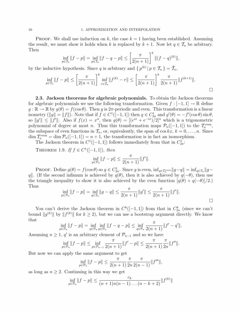
10 1. APPROXIMATION AND INTERPOLATION
Proof. We shall use induction on k, the case k = 1 having been established. Assumingthe result, we must show it holds when k is replaced by k + 1. Now let q ∈ Tn be arbitrary.Then
infp∈Tn
‖f − p‖ = infp∈Tn
‖f − q − p‖ ≤[
π
2(n+ 1)
]k
‖(f − q)(k)‖,
by the inductive hypothesis. Since q is arbitrary and p(k) | p ∈ Tn = Tn,
infp∈Tn
‖f − p‖ ≤[
π
2(n+ 1)
]k
infr∈Tn
‖f (k) − r‖ ≤[
π
2(n+ 1)
]kπ
2(n+ 1)‖f (k+1)‖.
2.3. Jackson theorems for algebraic polynomials. To obtain the Jackson theoremsfor algebraic polynomials we use the following transformation. Given f : [−1, 1]→ R defineg : R→ R by g(θ) = f(cos θ). Then g is 2π-periodic and even. This transformation is a linearisometry (‖g‖ = ‖f‖). Note that if f ∈ C1([−1, 1]) then g ∈ C1
2π and g′(θ) = −f ′(cos θ) sin θ,so ‖g′‖ ≤ ‖f ′‖. Also if f(x) = xn, then g(θ) = [(eix + e−ix)/2]n which is a trigonometricpolynomial of degree at most n. Thus this transformation maps Pn([−1, 1]) to the T even
n ,the subspace of even functions in Tn, or, equivalently, the span of cos kx, k = 0, . . . , n. Sincedim T even
n = dimPn([−1, 1]) = n+ 1, the transformation is in fact an isomorphism.The Jackson theorem in C1([−1, 1]) follows immediately from that in C1
2π:
Theorem 1.9. If f ∈ C1([−1, 1]), then
infp∈Pn
‖f − p‖ ≤ π
2(n+ 1)‖f ′‖.
Proof. Define g(θ) = f(cos θ) so g ∈ C12π. Since g is even, infq∈T even
n‖g−q‖ = infq∈Tn‖g−
q‖. (If the second infimum is achieved by q(θ), then it is also achieved by q(−θ), then usethe triangle inequality to show it is also achieved by the even function [q(θ) + q(−θ)]/2.)Thus
infp∈Pn
‖f − p‖ = infq∈Tn
‖g − q‖ ≤ π
2(n+ 1)‖g′‖ ≤ π
2(n+ 1)‖f ′‖.
You can’t derive the Jackson theorem in Ck([−1, 1]) from that in Ck2π (since we can’t
bound ‖g(k)‖ by ‖f (k)‖ for k ≥ 2), but we can use a bootstrap argument directly. We knowthat
infp∈Pn
‖f − p‖ = infq∈Pn
infp∈Pn
‖f − q − p‖ ≤ infq∈Pn
π
2(n+ 1)‖f ′ − q′‖.
Assuming n ≥ 1, q′ is an arbitrary element of Pn−1 and so we have
infp∈Pn
‖f − p‖ ≤ infp∈Pn−1
π
2(n+ 1)‖f ′ − p‖ ≤ π
2(n+ 1)
π
2n‖f ′′‖.
But now we can apply the same argument to get
infp∈Pn
‖f − p‖ ≤ π
2(n+ 1)
π
2n
π
2(n− 1)‖f ′′′‖,
as long as n ≥ 2. Continuing in this way we get
infp∈Pn
‖f − p‖ ≤ ck(n+ 1)n(n− 1) . . . (n− k + 2)
‖f (k)‖

2. MINIMAX POLYNOMIAL APPROXIMATION 11
if f ∈ Ck and n ≥ k − 1, with ck = (π/2)k. To state the result a little more compactly weanalyze the product M = (n + 1)n(n − 1) . . . (n − k + 2). Now if n ≥ 2(k − 2) then eachfactor is at least n/2, so M ≥ nk/2k. Also
dk := maxk−1≤n≤2(k−2)
nk
(n+ 1)n(n− 1) . . . (n− k + 2)<∞,
so, in all, nk ≤ ekM where ek = max(2k, dk). Thus we have arrived at the Jackson theoremin Ck:
Theorem 1.10. Let k be a positive integer, n ≥ k − 1 an integer. Then there exists aconstant c depending only on k such that
infp∈Pn
‖f − p‖ ≤ c
nk‖f (k)‖.
for all f ∈ Ck([−1, 1]).
2.4. Polynomial approximation of analytic functions. If a function is C∞ theJackson theorems show that the best polynomial approximation converges faster than anypower of n. If we go one step farther and assume that the function is analytic (i.e., itspower series converges at every point of the interval including the end points), we can proveexponential convergence.
We will first do the periodic case and show that the Fourier series for an analytic periodicfunction converges exponentially, and then use the Chebyshev transform to carry the resultover to the algebraic case.
A real function on an open interval is called real analytic if the function is C∞ and forevery point in the interval the Taylor series for the function about that point converges tothe function in some neighborhood of the point. A real function on a closed interval J isreal analytic if it is real analytic on some open interval containing J .
It is easy to see that a real function is real analytic on an interval if and only if it extendsto an analytic function on a neighborhood of the interval in the complex plane.
Suppose that g(z) is real analytic and 2π-periodic on R. Since g is smooth and periodicits Fourier series,
g(x) =∞∑
n=−∞
aneinx, an =
1
2π
∫ π
−π
g(x)e−inx dx,
converges absolutely and uniformly on R. Since g is real analytic, it extends to an analyticfunction on the strip Sδ := x + iy |x, y ∈ R, |y| ≤ δ for some δ > 0. Using analyticitywe see that we can shift the segment [−π, π] on which we integrate to define the Fouriercoefficients upward or downward a distance δ in the complex plane:
an =1
2π
∫ π
−π
g(x± iδ)e−in(x±iδ) dx =e±nδ
2π
∫ π
−π
g(x± iδ)e−inx dx.
Thus |an| ≤ ‖g‖L∞(Sδ)e−δ|n| and we have shown that the Fourier coefficients of a real analytic
periodic function decay exponentially.

12 1. APPROXIMATION AND INTERPOLATION
Now consider the truncated Fourier series q(z) =∑n
k=−n akeikz ∈ Tn. Then g(z)− q(z) =∑
|k|>n akeikz, so for any real z
|g(z)− q(z)| ≤∑|k|>n
|ak| ≤ 2‖g‖L∞(Sδ)
∞∑k=n+1
e−δk =2e−δ
1− e−δ‖g‖L∞(Sδ)e
−δn.
Thus we have proven:
Theorem 1.11. Let g be 2π-periodic and real analytic. Then there exist positive constantsC and δ so that
infq∈Tn
‖g − q‖∞ ≤ Ce−δn.
The algebraic case follows immediately from the periodic one. If f is real analytic on[−1, 1], then g(θ) = f(cos θ) is 2π-periodic and real analytic. Since infq∈Tn‖g − q‖∞ =infq∈T even
n‖g − q‖∞ = infp∈Pn‖f − p‖∞, we can apply the previous result to bound the latter
quantity by Ce−δn.
Theorem 1.12. Let f be real analytic on a closed interval. Then there exist positiveconstants C and δ so that
infp∈Pn
‖f − p‖∞ ≤ Ce−δn.
2.5. Characterization of the minimax approximant. Having established the rateof approximation afforded by the best polynomial approximation with respect to the L∞
norm, in this section we derive two conditions that characterize the best approximation.We will use these results to show that the best approximation is unique (recall that ouruniqueness theorem in the first section only applied to strictly convex norms, and so excludedthe case of L∞ approximation). The results of this section can also be used to design iterativealgorithms which converge to the best approximation, but we shall not pursue that, becausethere are approximations which yield nearly as good approximation in practice as the bestapproximation but which are much easier to compute.
The first result applies very generally. Let J be an compact subset of Rn (or even ofa general Hausdorff topological space), and let P be any finite dimensional subspace ofC(J). For definiteness you can think of J as a closed interval and P as the space Pn(J) ofpolynomials of degree at most n, but the result doesn’t require this.
Theorem 1.13 (Kolmogorov Characterization Theorem). Let f ∈ C(J), P a finitedimensional subspace of C(J), p ∈ P . Then p is a best approximation to f in P if and onlyif no element of P has the same sign as f − p on its extreme set.
Proof. First we note that p is a best approximation to f in P if and only if 0 is a bestapproximation to g := f − p in P . So we need to show that 0 is a best approximation to gif and only if no element q of P has the same sign as g on its extreme set.
First suppose that 0 is not a best approximation. Then there exists q ∈ P such that‖g − q‖ < ‖g‖. Now let x be a point in the extreme set of g. Unless sign q(x) = sign g(x),|g(x) − q(x)| ≥ |g(x)| = ‖g‖, which is impossible. Thus q has the same sign of as g on itsextreme set.
The converse direction is trickier, but the idea is simple. If q has the same sign of asg on its extreme set and we subtract a sufficiently small positive multiple of q from g, the

2. MINIMAX POLYNOMIAL APPROXIMATION 13
difference will be of strictly smaller magnitude than g near the extreme set. And if themultiple that we subtract is small enough the difference will also stay below the extremevalue away from the extreme set. Thus g − εq will be smaller than g for ε small enough, sothat 0 is not the best approximation.
Since we may replace q by q/‖q‖ we can assume from the outset that ‖q‖ = 1. Let δ > 0be the minimum of qg on the extreme set, and set S = x ∈ J | q(x)g(x) > δ/2, so that Sis an open set containing the extreme set. Let M = maxJ\S|g| < ‖g‖.
Now on S, qg > δ/2, so
|g − εq|2 = |g|2 − 2εqg + ε2|q|2 ≤ ‖g‖2 − εδ + ε2 = ‖g‖2 − ε(δ − ε),
and so if 0 < ε < δ then ‖g − εq‖∞,S < ‖g‖.On J \ S, |g − εq| ≤M + |ε|, so if 0 < ε < ‖g‖ −M , ‖g − εq‖∞,J\S < ‖g‖. Thus for any
positive ε sufficiently small ‖g − εq‖ < ‖g‖ on J .
While the above result applies to approximation by any finite dimensional subspace P ,we now add the extra ingredient that P = Pn([a, b]) the space of polynomial functions ofdegree at most n on a compact interval J = [a, b].
Theorem 1.14 (Chebyshev Alternation Theorem). Let f ∈ C([a, b]), p ∈ Pn. Then pis a best approximation to f in Pn if and only if f − p achieves its maximum magnitude atn+ 2 distinct points with alternating sign.
Proof. If f−p achieves its maximum magnitude at n+2 distinct points with alternatingsign, then certainly no function q ∈ Pn has the same sign as f − p on its extreme set (sincea nonzero element of Pn cannot have n+ 1 zeros). So p is a best approximation to f in Pn.
Conversely, suppose that f − p changes sign at most n+ 1 times on its extreme set. Fordefiniteness suppose that f − p is positive at its first extreme point. Then we can choosen points x1 < x2 < · · ·xn in [a, b] such that f − p is positive on extreme points less thanx1, negative on extreme points in on [x1, x2], positive on extreme points in [x2, x3], etc. Thefunction q(x) = (x1 − x) · · · (xn − x) ∈ Pn then has the same sign as f − p on its extremeset, and so p is not a best approximation to f in Pn.
The Chebyshev Alternation Theorem is illustrated in Figure 1.5.We can now prove uniqueness of the best approximation.
Corollary 1.15. The best L∞ approximation to a continuous function by a function inPn is unique.
Proof. Suppose p, p∗ ∈ Pn are both best approximations to f . Let e = f−p, e∗ = f−p∗,and say M = ‖e‖ = ‖e∗‖. Since (p + p∗)/2 is also a best approximation, |f − (p + p∗)/2|achieves the value M at n+ 2 points, x0, . . . , xn+1. Thus
M = |[e(xi) + e∗(xi)]/2| ≤ |e(xi)|/2 + |e∗(xi)|/2 ≤M.
Thus equality holds throughout, and e(xi) = e∗(xi), so p(xi) = p∗(xi) at all n + 2 points,which implies that p = p∗.
Remarks. 1. The only properties we used of the space Pn are (1) that no non-zeroelement has more than n zeros, and (2) given any n points there is an element with exactly

14 1. APPROXIMATION AND INTERPOLATION
Figure 1.5. A sinusoidal function and its minimax approximation of degrees3 and 4. The error curves, on the right, achieve their maximal magnitudes atthe requisite 5 and 6 points, respectively.
−1 −0.5 0 0.5 1
−1
0
1
degree 3
−1 −0.5 0 0.5 1
−.33
0
.33
error
−1 −0.5 0 0.5 1
−1
0
1
degree 4
−1 −0.5 0 0.5 1
−.1
0
.1
error
those points as the zeros. These two conditions together (which are equivalent to the exis-tence and uniqueness of an interpolant at n+ 1 points, as discussed in the next section) arereferred to as the Haar property. Many other subspaces satisfy the Haar property, and sowe can obtain a Chebyshev Alternation Theorem for them as well.
2. The Chebyshev alternation characterization of the best approximation can be usedas the basis for a computational algorithm to approximate the best approximation, knownas the exchange algorithm or Remes algorithm. However in practice something like theinterpolant at the Chebyshev points, which, as we shall see, is easy to compute and usuallygives something quite near best approximation, is much more used.
3. Lagrange Interpolation
3.1. General results. Now we consider the problem of not just approximating, butinterpolating a function at given points by a polynomial. That is, we suppose given n + 1distinct points x0 < x1 < · · · < xn and n + 1 values y0, y1, . . . , yn. We usually think of theyi as the value f(xi) of some underlying function f , but this is not necessary. In any case,there exists a unique polynomial p ∈ Pn such that p(xi) = yi. To prove this, we notice that ifwe write p =
∑ni=0 cix
i, then the interpolation problem is a system of n+ 1 linear equationsin the n + 1 unknowns ci. We wish to show that this system is non-singular. Were it not,there would exists a non-zero polynomial in Pn vanishing at the xi, which is impossible, and
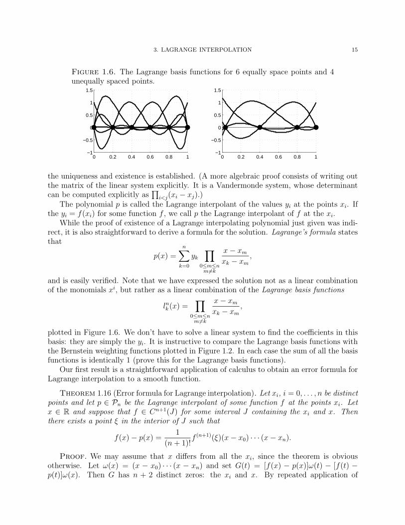
3. LAGRANGE INTERPOLATION 15
Figure 1.6. The Lagrange basis functions for 6 equally space points and 4unequally spaced points.
0 0.2 0.4 0.6 0.8 1−1
−0.5
0
0.5
1
1.5
0 0.2 0.4 0.6 0.8 1−1
−0.5
0
0.5
1
1.5
the uniqueness and existence is established. (A more algebraic proof consists of writing outthe matrix of the linear system explicitly. It is a Vandermonde system, whose determinantcan be computed explicitly as
∏i<j(xi − xj).)
The polynomial p is called the Lagrange interpolant of the values yi at the points xi. Ifthe yi = f(xi) for some function f , we call p the Lagrange interpolant of f at the xi.
While the proof of existence of a Lagrange interpolating polynomial just given was indi-rect, it is also straightforward to derive a formula for the solution. Lagrange’s formula statesthat
p(x) =n∑
k=0
yk
∏0≤m≤n
m6=k
x− xm
xk − xm
,
and is easily verified. Note that we have expressed the solution not as a linear combinationof the monomials xi, but rather as a linear combination of the Lagrange basis functions
lnk (x) =∏
0≤m≤nm6=k
x− xm
xk − xm
,
plotted in Figure 1.6. We don’t have to solve a linear system to find the coefficients in thisbasis: they are simply the yi. It is instructive to compare the Lagrange basis functions withthe Bernstein weighting functions plotted in Figure 1.2. In each case the sum of all the basisfunctions is identically 1 (prove this for the Lagrange basis functions).
Our first result is a straightforward application of calculus to obtain an error formula forLagrange interpolation to a smooth function.
Theorem 1.16 (Error formula for Lagrange interpolation). Let xi, i = 0, . . . , n be distinctpoints and let p ∈ Pn be the Lagrange interpolant of some function f at the points xi. Letx ∈ R and suppose that f ∈ Cn+1(J) for some interval J containing the xi and x. Thenthere exists a point ξ in the interior of J such that
f(x)− p(x) =1
(n+ 1)!f (n+1)(ξ)(x− x0) · · · (x− xn).
Proof. We may assume that x differs from all the xi, since the theorem is obviousotherwise. Let ω(x) = (x − x0) · · · (x − xn) and set G(t) = [f(x) − p(x)]ω(t) − [f(t) −p(t)]ω(x). Then G has n + 2 distinct zeros: the xi and x. By repeated application of

16 1. APPROXIMATION AND INTERPOLATION
Rolle’s theorem there exists a point ξ strictly between the largest and the smallest of thezeros such that d(n+1)G/dt(n+1)(ξ) = 0. Since p(n+1) ≡ 0 and ω(n+1) ≡ (n + 1)!, this gives[f(x)− p(x)](n+ 1)!− f (n+1)(ξ)ω(x) which is the desired result.
Remark. If all the xi tend to the same point a, then p tends to the Taylor polynomialof degree n at a, and the estimate tends to the standard remainder formula for the Taylorpolynomial: f(x)− p(x) = [1/(n+ 1)!]f (n+1)(ξ)(x− a)n+1 for some ξ between x and a.
An obvious corollary of the error formula is the estimate:
|f(x)− p(x)| ≤ 1
(n+ 1)!‖f (n+1)‖∞,J |ω(x)|.
In particular
|f(x)− p(x)| ≤ 1
(n+ 1)!‖f (n+1)‖∞,Jk
n+1,
where k = max(|x− xi|, |xi − xj|). In particular if a ≤ minxi, b ≥ maxxi, then
(1.3) ‖f − p‖∞,[a,b] ≤1
(n+ 1)!‖f (n+1)‖∞,[a,b]|b− a|n+1,
no matter what the configuration of the points xi ∈ [a, b]. This gives a useful estimate ifwe hold n fixed and let the points xi tend to the evaluation point x. It establishes a rate ofconvergence of order n+ 1 with respect to the interval length for Lagrange interpolation atn+ 1 points in the interval.
Another interesting question, closer to the approximation problem we have consideredheretofore, asks about the error on a fixed interval as we increase the number of interpolationpoints and so the degree of the interpolating polynomial. At this point we won’t restrict theconfiguration of the points, so we consider an arbitrary tableau of points
x00
x10 < x1
1
x20 < x2
1 < x22
...
all belonging to [a, b]. Then we let pn ∈ Pn interpolate f at xni , i = 0, . . . , n and inquire
about the convergence of pn to fn as n → ∞. Whether such convergence occurs, and howfast, depends on the properties of the function f and on the particular arrangement of points.
One possibility is to make a very strong assumption on f , namely that f is real analyticon [a, b]. Now if f is analytic on the closed disk B(ξ, R) of radius R about ξ, then, byCauchy’s estimate, |f (n+1)(ξ)| ≤ (n + 1)!‖f‖∞,B(ξ,R)/R
n+1. Let O(a, b, R) denote the oval⋃ξ∈[a,b] B(ξ, R). We then have
Theorem 1.17. Let a < b and suppose that f extends analytically to the oval O(a, b, R)for some R > 0. Let x0 < · · · < xn be any set of n + 1 distinct points in [a, b] and let p bethe Lagrange interpolating polynomial to f at the xi. Then
‖f − p‖∞,[a,b] ≤ ‖f‖∞,O(a,b,R)
(|b− a|R
)n+1
.
3. LAGRANGE INTERPOLATION 17
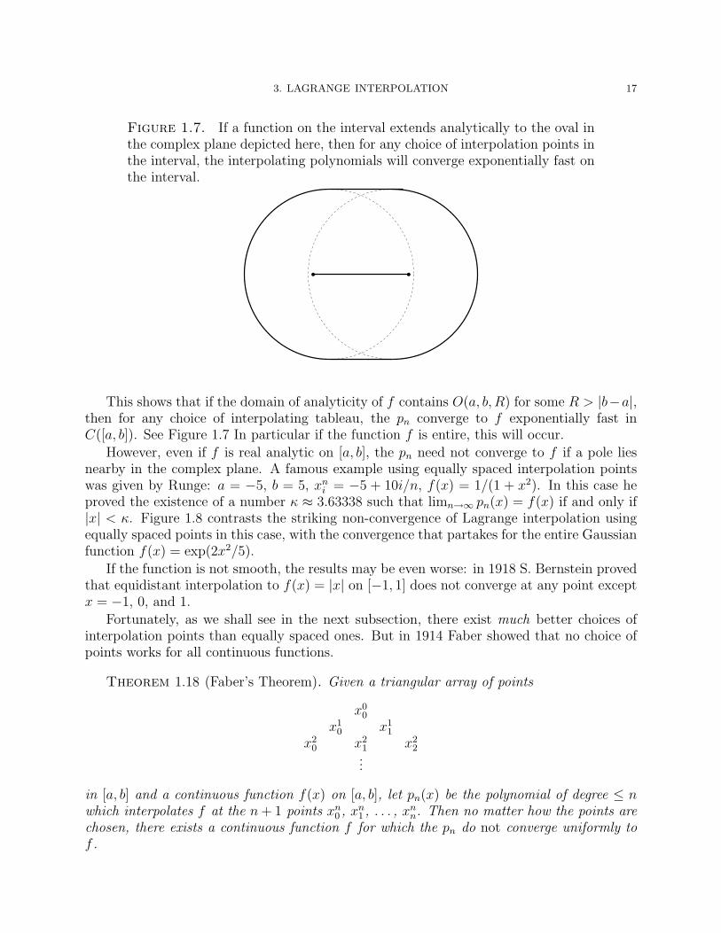
Figure 1.7. If a function on the interval extends analytically to the oval inthe complex plane depicted here, then for any choice of interpolation points inthe interval, the interpolating polynomials will converge exponentially fast onthe interval.
This shows that if the domain of analyticity of f contains O(a, b, R) for some R > |b−a|,then for any choice of interpolating tableau, the pn converge to f exponentially fast inC([a, b]). See Figure 1.7 In particular if the function f is entire, this will occur.
However, even if f is real analytic on [a, b], the pn need not converge to f if a pole liesnearby in the complex plane. A famous example using equally spaced interpolation pointswas given by Runge: a = −5, b = 5, xn
i = −5 + 10i/n, f(x) = 1/(1 + x2). In this case heproved the existence of a number κ ≈ 3.63338 such that limn→∞ pn(x) = f(x) if and only if|x| < κ. Figure 1.8 contrasts the striking non-convergence of Lagrange interpolation usingequally spaced points in this case, with the convergence that partakes for the entire Gaussianfunction f(x) = exp(2x2/5).
If the function is not smooth, the results may be even worse: in 1918 S. Bernstein provedthat equidistant interpolation to f(x) = |x| on [−1, 1] does not converge at any point exceptx = −1, 0, and 1.
Fortunately, as we shall see in the next subsection, there exist much better choices ofinterpolation points than equally spaced ones. But in 1914 Faber showed that no choice ofpoints works for all continuous functions.
Theorem 1.18 (Faber’s Theorem). Given a triangular array of points
x00
x10 x1
1
x20 x2
1 x22
...
in [a, b] and a continuous function f(x) on [a, b], let pn(x) be the polynomial of degree ≤ nwhich interpolates f at the n+ 1 points xn
0 , xn1 , . . . , xn
n. Then no matter how the points arechosen, there exists a continuous function f for which the pn do not converge uniformly tof .

18 1. APPROXIMATION AND INTERPOLATION
Figure 1.8. Interpolation by polynomials of degree 16 using equally spacedinterpolation points. The first graph shows Runge’s example. In the secondgraph, the function being interpolated is entire, and the graph of the interpo-lating polynomial nearly coincides with that of the function.
−5 0 5−0.5
0
0.5
1
1.5Runge’s example
−5 0 5−0.5
0
0.5
1
1.5interpolation of a Gaussian
In 1931 Bernstein strengthened this negative theorem to show that there exists a con-tinuous function f and a point c in [a, b] for which pn(c) does not converge to f(c). In 1980Erdos and Vertesi showed that in fact there exists a continuous function f such that pn(c)does not converge to f(c) for almost all c in [a, b].
However, as we shall now show, if the function f is required to have a little smoothness,and if the interpolation points are chosen well, then convergence will be obtained.
3.2. The Lebesgue constant. Given n + 1 distinct interpolation points in [a, b] andf ∈ C([a, b]), let Pnf ∈ Pn be the Lagrange interpolating polynomial. Then Pn is an operatorfrom C([a, b]) to itself, and we may consider its norm:
‖Pn‖ = supf∈C([a,b])‖f‖∞≤1
‖Pnf‖∞.
Using this norm, it is easy to relate the error in interpolation to the error in best approxi-mation:
‖f − Pnf‖ = infq∈Pn
‖f − q − Pn(f − q)‖ ≤ (1 + ‖Pn‖) infq∈Pn
‖f − q‖.
Note that the only properties of Pn we have used to get this estimate are linearity and thefact that it preserves Pn.
Thus, if we can bound ‖Pn‖ we can obtain error estimates for interpolation from thosefor best approximation (i.e., the Jackson theorems). Now let
lnk (x) =∏
0≤m≤nm6=k
x− xm
xk − xm

3. LAGRANGE INTERPOLATION 19
Figure 1.9. Lebesgue function for degree 8 interpolation at equally spaced points.
0 0.1 0.2 0.3 0.4 0.5 0.6 0.7 0.8 0.9 1−4
−2
0
2
4
6
8
10
12
denote the Lagrange basis functions. Recall that∑n
k=0 lnk (x) = 1. Set
Ln(x) =n∑
k=0
|lnk (x)|,
the Lebesgue function for this choice of interpolation points. Then
‖Pn‖ = sup0≤x≤1
sup|f |≤1
∣∣∣∣∣n∑
k=0
f(xk)lnk (x)
∣∣∣∣∣ = sup0≤x≤1
n∑k=0
|lnk (x)| = ‖Ln‖∞.
Figure 1.9 shows the Lebesgue function for interpolation by a polynomial of degree 8 us-ing equally spaced interpolation points plotted together with the Lagrange basis functionsentering into its definition.
The constant ‖Pn‖ = ‖Ln‖∞ is called the Lebesgue constant of the interpolation opera-tor. Of course it depends on the point placement. However it only depends on the relativeconfiguration: if we linearly scale the points from the interval [a, b] to another interval, thenthe constant doesn’t change. Table 1.1 shows the Lebesgue constants for equally spacedinterpolation points ranging from a to b. Note that the constant grows quickly with n re-flecting the fact that the approximation afforded by the interpolant may be much worse thanthe best approximation. The column labelled “Chebyshev” shows the Lebesgue constant if abetter choice of points, the Chebyshev points, is used. We study this in the next subsection.
It is not clear from the table whether the Lebesgue constant remains bounded for inter-polation at the Chebyshev points, but we know it does not: otherwise the Chebyshev pointswould give a counterexample to Faber’s theorem. In fact Erdos proved a rather precise lowerbound on growth rate.
Theorem 1.19. [Erdos 1961] For any triangular array of points, there is a constant csuch that corresponding Lebesgue constant satisfies
‖Pn‖ ≥2
πlog n− c.
This result was known well earlier, but with a less precise constant. See, e.g., Rivlin’sIntroduction to the Approximation of Functions [5] for an elementary argument.

20 1. APPROXIMATION AND INTERPOLATION
Table 1.1. Lebesgue constants for interpolation into Pn at equally spacedpoints and Chebyshev points (to three significant digits).
n Equal Chebyshev2 1.25 1.674 2.21 1.996 4.55 2.208 11.0 2.3610 29.9 2.4912 89.3 2.6014 283 2.6916 935 2.7718 3,170 2.8420 11,000 2.90
3.3. The Chebyshev points. Returning to the error formula for Lagrange interpola-tion we see that a way to reduce the error is to choose the interpolation points xi so as todecrease ω(x) = (x− x0) . . . (x− xn). Assuming that we are interested in reducing the erroron all of [a, b], we are led to the problem of finding x0 < · · · < xn which minimize
(1.4) supa≤x≤b
|(x− x0) . . . (x− xn)|.
In fact, we can solve this problem in closed form. First consider the case [a, b] = [−1, 1].Define Tn(x) = cos(n arccos x) ∈ Pn([−1, 1]), the polynomial which corresponds to cosnθunder the Chebyshev transform. Tn is called the nth Chebyshev polynomial:
T0(x) = 1, T1(x) = x, T2(x) = 2x2 − 1, T3(x) = 4x3 − 3x, T4(x) = 8x4 − 8x2 + 1, . . .
Using trigonometric identities for cos(n± 1)x, we get the recursion relation
Tn+1(x) = 2xTn(x)− Tn−1(x),
from which it easily follows that Tn(x) is a polynomial of exact degree n with leading coef-ficient 2n−1.
Now let xni = cos[(2i + 1)π/(2n + 2)]. Then it is easy to see that 1 > xn
0 > xn1 > · · · >
xnn > −1 and that these are precisely the n + 1 zeros of Tn+1. These are called the n + 1
Chebyshev points on [−1, 1]. The definition is illustrated for n = 8 in Figure 1.10. The nexttheorem shows that the Chebyshev points minimize (1.4).
Theorem 1.20. For n ≥ 0, let x0, x1, . . . xn ∈ R and set ω(x) = (x − x0) . . . (x − xn).Then
supa≤x≤b
|ω(x)| ≥ 2−n,
and if xi = cos[(2i+ 1)π/(2n+ 2)], then
supa≤x≤b
|ω(x)| = 2−n.
Proof. First assume that the xi are the n+1 Chebyshev points. Then ω and Tn+1 are twopolynomials of degree n+1 with the same roots. Comparing their leading coefficients we seethat ω(x) = 2−nTn+1(x) = 2−n cos(n arccos x). The second statement follows immediately.

3. LAGRANGE INTERPOLATION 21
Figure 1.10. The Chebyshev points x8i = cos[(2i+ 1)π/18].
Note also that for this choice of points, |ω(x)| achieves its maximum value of 2−n at n + 2distinct points in [−1, 1], namely at cos[jπ/(n + 1)], j = 0, . . . , n + 1, and that the sign ofω(x) alternates at these points.
Now suppose that some other points xi are given and set ω(x) = (x− x0) · · · (x− xn). If|ω(x)| < 2−n on [−1, 1], then ω(x)− ω(x) alternates sign at the n+ 2 points cos[jπ/(n+ 1)]and so has at least n+ 1 zeros. But it is a polynomial of degree at most n (since the leadingterms cancel), and so must vanish identically, a contradiction.
Table 1.1 indicates the Lebesgue constant for Chebyshev interpolation grows rather slowlywith the degree (although it does not remain bounded). In fact the rate of growth is onlylogarithmic and can be bounded very explicitly. See [6] for a proof.
Theorem 1.21. If Pn : C([a, b]) → Pn([a, b]) denotes interpolation at the Chebyshevpoints, then
‖Pn‖ ≤2
πlog(n+ 1) + 1, n = 0, 1, . . . .
Comparing with Theorem 1.19, we see that Chebyshev interpolation gives asymptoticallythe best results possible. Combining this result with the Jackson theorems we see that Cheby-shev interpolation converges for any function C1, and if f ∈ Ck, then ‖f−Pn‖ ≤ Cn−k log n,so the rate of convergence as n→∞ is barely worse than for the best approximation. Usingthe Jackson theorem for Holder continuous functions (given in the exercises), we see that in-deed Chebyshev interpolation converges for any Holder continuous f . Of course, by Faber’stheorem, there does exist a continuous function for which it doesn’t converge, but that func-tion must be quite unsmooth. We can summarize this by saying that Chebyshev interpolationis a robust approximation procedure (it converges for any “reasonable” continuous function)and an accurate one (it converges quickly if the function is reasonably smooth). Comparethis with Bernstein polynomial approximation which is completely robust (it converges forany continuous function), but not very accurate.
Figure 1.11 repeats the example of best approximation from Figure 1.5, but adds theChebyshev interpolant. We see that, indeed, on this example the Chebyshev interpolant isnot far from the best approximation and the error not much larger than the error in bestapproximation.

22 1. APPROXIMATION AND INTERPOLATION
Figure 1.11. The sinusoidal function and its minimax approximation(shown with a dotted line) of degrees 3 and 4 and the corresponding errorcurves, as in Figure 1.5. The thin lines show the interpolant at the Chebyshevpoints and the error curves for it.
−1 −0.5 0 0.5 1
−1
0
1
degree 3
−1 −0.5 0 0.5 1
−.33
0
.33
error
−1 −0.5 0 0.5 1
−1
0
1
degree 4
−1 −0.5 0 0.5 1
−.1
0
.1
error
4. Least Squares Polynomial Approximation
4.1. Introduction and preliminaries. Now we consider best approximation in thespace L2([a, b]). The key property of the L2 norm which distinguishes it from the other Lp
norms, is that it is determined by an inner product, 〈u, v〉 =∫ b
au(x)v(x) dx.
Definition. A normed vector space X is an inner product space if there exists a sym-metric bilinear form 〈 · , · 〉 on X such that ‖x‖2 = 〈x, x〉.
Theorem 1.22. Let X be an inner product space, P be a finite dimensional subspace,and f ∈ X. Then there exists a unique p ∈ P minimizing ‖f−p‖ over P . It is characterizedby the normal equations
〈p, q〉 = 〈f, q〉, q ∈ P.
Proof. We know that there exists a best approximation p. To obtain the character-ization note that ‖f − p + εq‖2 = ‖f − p‖2 + 2ε〈f − p, q〉 + ε2‖q‖2 achieves its minimum(as a quadratic polynomial in ε) at 0. If p and p∗ are both best approximation the normalequations give 〈p− p∗, q〉 = 0 for q ∈ P . Taking q = p− p∗ shows p = p∗. (Alternative proofof uniqueness: show that an inner product space is always strictly convex.)

4. LEAST SQUARES POLYNOMIAL APPROXIMATION 23
In the course of the proof we showed that the normal equations admit a unique solution.To obtain the solution, we select a basis φ1, . . . , φn of P , write p =
∑j ajφj, and solve the
equationsn∑
j=1
〈φj, φi〉aj = 〈f, φi〉, i = 1, . . . , n.
This is a nonsingular matrix equation.Consider as an example the case where X = L2([0, 1]) and P = Pn. If we use the
monomials as a basis for Pn, then the matrix elements are∫ 1
0xjxi dx = 1/(i + j + 1). In
other words the matrix is the Hilbert matrix, famous as an example of a badly conditionedmatrix. Thus this is not a good way to solve the normal equations.
Suppose we can find another basis for P which is orthogonal: 〈Pj, Pi〉 = 0 if i 6= j. In thatcase the matrix system is diagonal and trivial to solve. But we may construct an orthogonalbasis Pi starting from any basis φi using the Gram-Schmidt process: P1 = φ1,
Pj = φj −j−1∑k=1
〈φj, Pk〉‖Pk‖2
Pk, j = 2, . . . , n.
Note that for an orthogonal basis we have the simple formula
p =n∑
j=1
cjPj, cj =〈f, Pj〉‖Pj‖2
.
If we normalize the Pj so that ‖Pj‖ = 1 the formula for cj simplifies to cj = 〈f, Pj〉
4.2. The Legendre polynomials. Consider now the case of X = L2([a, b]), P =Pn([a, b]). Applying the Gram-Schmidt process to the monomial basis we get a sequenceof polynomials pn = xn + lower with pn ⊥ Pn−1. This is easily seen to characterize the pn
uniquely.The Gram-Schmidt process simplifies for polynomials. For the interval [−1, 1] define
p0(x) = 1,
p1(x) = x,
pn(x) = xpn−1(x)−〈xpn−1, pn−2〉‖pn−2‖2
pn−2(x), n ≥ 2.
It is easy to check that these polynomials are monic and orthogonal. The numerator in thelast equation is equal to ‖pn−1‖2. These polynomials, or rather constant multiples of them,are called the Legendre polynomials.
p0(x) = 1,
p1(x) = x,
p2(x) = x2 − 1/3,
p3(x) = x3 − 3x/5.
We can obtain the Legendre polynomials on an arbitrary interval by linear scaling.

24 1. APPROXIMATION AND INTERPOLATION
We normalized the Legendre polynomials by taking their leading coefficient as 1. Morecommonly the Legendre polynomials are normalized to have value 1 at 1. Then it turns outthat the recursion can be written
(n+ 1)Pn+1(x) = (2n+ 1)xPn(x)− nPn−1(x),
starting with P0 = 1, P1(x) = x (see [5], Ch. 2.2 for details). Henceforth we shall use Pn
to denote the Legendre polynomials so normalized. Now we shall gather some properties ofthem (see [5] Ch. 2, including the exercises, for details).
0) Pn(1) = 1, Pn(−1) = (−1)n, Pn is even or odd according to whether n is even or odd.1) ‖Pn‖2 = 2/(2n+ 1).2) The leading coefficient of Pn = (2n− 1)(2n− 3) · · · 1/n! = (2n)!/[2n(n!)2].3) It is easy to check, by integration by parts, that the functions dn
dxn [(x2 − 1)n] arepolynomials of degree n and are mutually orthogonal. Comparing leading coefficients we getRodrigues’s formula for Pn:
Pn =1
2nn!
dn
dxn[(x2 − 1)n].
4) Using Rodrigues’s formula one can show, with some tedious manipulations, that
d
dx
[(x2 − 1)
dPn
dx
]= n(n+ 1)Pn,
i.e., the Pn are the eigenfunctions of the given differential operator.5) Using this equation one can prove that |Pn| ≤ 1 on [−1, 1] (see Isaacson & Keller,
Ch. 5, Sec. 3, problem 8).6) Pn has n simple roots, all in (−1, 1). Indeed to prove this, it suffices to show that
Pn changes sign at n points in (−1, 1). If the points where Pn changes sign in (−1, 1) arex1, . . . , xk, then Pn isn’t orthogonal to (x− x1) · · · (x− xk), so k ≥ n.
Using the Legendre polynomials to compute the least squares approximation has theadditional advantage that if we increase the degree the polynomial approximation changesonly by adding additional terms: the coefficients of the terms already present don’t change.
Now consider the error f −∑cjPj. We have
‖f −n∑
j=0
cjPj‖2 = ‖f‖2 +n∑
j=0
c2j‖Pj‖2 − 2n∑
j=0
cj〈f, Pj〉.
But 〈f, Pj〉 = cj‖Pj‖2, so
‖f −∑
cjPj‖2 = ‖f‖2 −n∑
j=0
c2j‖Pj‖2
In particular, this shows that∑n
j=0 c2j‖Pj‖2 is bounded above by ‖f‖2 for all n, so the limit∑∞
j=0 c2j‖Pj‖2 exists. In fact this limit must equal ‖f‖2, since if it were strictly less than ‖f‖2
we would have ‖f −∑n
j=0 cjPj‖ ≥ δ for some δ > 0 and all n, i.e., infp∈Pn‖f −p‖2 ≥ δ for all
n. But, infp∈Pn‖f − p‖22 ≤ infp∈Pn‖f − p‖2∞, and the latter tends to zero by the WeierstrassApproximation Theorem.

4. LEAST SQUARES POLYNOMIAL APPROXIMATION 25
Theorem 1.23. Let f ∈ C([a, b]) and let Pn be the orthogonal polynomials on [a, b] (withany normalization). Then the best approximation to f in Pn with respect to the L2 norm isgiven by
(1.5) pn =n∑
j=0
cjPj, cn =〈f, Pj〉‖Pj‖2
.
The L2 error is given by
‖f − pn‖2 = ‖f‖2 −n∑
j=0
c2j‖Pj‖2 = ‖f‖2 − ‖pn‖2
and this quantity tends to zero as n tends to infinity. In particular
‖f‖2 =∞∑
j=0
c2j‖Pj‖2.
The last equation is Parseval’s equality. It depended only on the orthogonality of thePn and on the completeness of the polynomials (any continuous function can be representedarbitrarily closely in L2 by a polynomial).
4.3. Error analysis. We now consider the rate of convergence of pn, the best L2 approx-imation of f , to f . An easy estimate follows from the fact that ‖f‖L2([−1,1] ≤
√2‖f‖L∞([−1,1]):
infp∈Pn
‖f − p‖2 ≤√
2 infp∈Pn
‖f − p‖∞.
The right-hand side can be bounded Jackson’s theorems, e.g., by ckn−k‖f (k)‖∞.
Another interesting question is whether pn converges to f in L∞. For this we will computethe Lebesgue constant for best L2 approximation. That is we shall find a number cn suchthat ‖pn‖∞ ≤ cn‖f‖∞ whenever pn is the best L2 approximation of f in Pn. It then followsthat ‖f − pn‖∞ ≤ (1 + cn) infq∈Pn‖f − q‖∞, and again we can apply the Jackson theoremsto bound the right-hand side. Now we know that all norms on the finite dimensional spacePn are equivalent, so there is a constant Kn such that ‖q‖∞ ≤ Kn‖q‖2 for all q ∈ Pn. Then
‖pn‖∞ ≤ Kn‖pn‖2 ≤ Kn‖f‖2 ≤√
2Kn‖f‖∞,and so the Lebesgue constant is bounded by
√2Kn. To get a value for Kn, we write an arbi-
trary element of Pn as q =∑n
k=0 akPk. Then ‖q‖∞ ≤∑n
k=0 |ak|, and ‖q‖22 =∑n
k=0 |ak|2 22k+1
.Thus for the best choice for Kn,
K2n = max
(∑n
k=0 |ak|)2∑nk=0 |ak|2 2
2k+1
.
We can find the maximum using the Cauchy-Schwarz inequality:
(n∑
k=0
|ak|)2 = (n∑
k=0
(|ak|√
2
2k + 1)
√2k + 1
2)2 ≤
(n∑
k=0
|ak|22
2k + 1
)(n∑
k=0
2k + 1
2
).
Thus K2n ≤
∑nk=0
2k+12
= (n+1)2
2. We have thus shown that ‖q‖∞ ≤ (n + 1)/
√2‖q‖2 for
q ∈ Pn, the Lebesgue constant of least squares approximation in Pn is bounded by n + 1and, consequently, for any function f for which the best L∞ approximation converges faster

26 1. APPROXIMATION AND INTERPOLATION
than O(1/n), the best L2 approximation converges in L∞, with at most one lower rate ofconvergence.
4.4. Weighted least squares. The theory of best approximation in L2 extends to bestapproximation in the weighted norm
‖f‖w,2 :=
(∫ b
a
|f(x)|2w(x) dx
)1/2
,
where w : (a, b) → R+ is an integrable function. The point is, this norm arises from aninner product, and hence most of theory developed above goes through (one thing that doesnot go through, is that unless the interval is symmetric with respect to the origin and w iseven, it will not be the case that the orthogonal polynomials will alternate odd and even
parity). Writing 〈f, g〉 =∫ b
af(x)g(x)w(x) dx for the inner product, we define orthogonal
polynomials by a modified Gram-Schmidt procedure as follows. Let Q0(x) ≡ 1. DefineQ1 = xQ0− a0Q0 where a0 is chosen so that 〈Q1, Q0〉 = 0, i.e., a0 = 〈xQ0, Q0〉/‖Q0‖2. ThenQ2 = xQ1 − a1Q1 − b1Q0 where a1 is chosen so that 〈Q2, Q1〉 = 0 (a1 = 〈xQ1, Q1〉/‖Q1‖2)and b1 is chosen so that 〈Q2, Q0〉 = 0 (b1 = 〈(x − a1)Q1, Q0〉/‖Q0‖2. We then defineQ3 = xQ2− a2Q2− b2Q1, choosing a2 and b2 to get orthogonality to Q2 and Q1 respectively.Each of the terms on the right-hand side is individually orthogonal to Q0, so this procedureworks, and can be continued. In summary:
Qn+1 = (x− an)Qn − bnQn−1, an =〈xQn, Qn〉‖Qn‖2
, bn =〈(x− an)Qn, Qn−1〉
‖Qn−1‖2.
Actually, 〈(x − an)Qn, Qn−1〉 = ‖Qn‖2, since Qn = (x − a)Qn−1 + · · · , so we can writebn = ‖Qn‖2/‖Qn−1‖.
This gives the orthogonal polynomials for the weight w on [a, b] normalized so as to bemonic. As for the Legendre polynomials other normalizations may be more convenient.
Probably the most important case is w(x) = 1/√
1− x2, in which case we get the Cheby-shev polynomials Tn as orthogonal polynomials. To see that these are L2([−1, 1], w) orthog-onal make the change of variables x = cos θ, 0 < θ < π to get∫ 1
−1
Tn(x)Tm(x)1√
1− x2dx =
∫ π
0
cosnθ cosmθ dθ.
The recurrence relation is, as we have already seen, is
Tn+1 = 2xTn − Tn−1, T0 = 1, T1 = x.
Other famous families of orthogonal polynomials are: Chebyshev of second kind (weightof√
1− x2 on [−1, 1]), Jacobi (weight of (1−x)α(1+x)β on [−1, 1]) which contains the threepreceding cases as special cases, Laguerre (weight of e−x on [0,∞), and Hermite (weight of
e−x2on R).
5. Piecewise polynomial approximation and interpolation
If we are given a set of distinct points on an interval and values to impose at thosepoints, we can compute the corresponding Lagrange interpolating polynomial. However weknow, e.g., from Runge’s example, that for more than a few points, this polynomial maybe highly oscillatory even when the values are taken from a smooth underlying function.
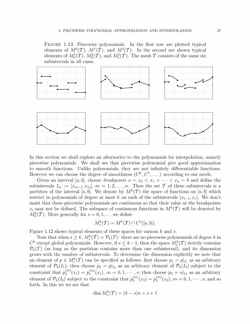
5. PIECEWISE POLYNOMIAL APPROXIMATION AND INTERPOLATION 27
Figure 1.12. Piecewise polynomials. In the first row are plotted typicalelements of M0(T ), M1(T ), and M2(T ). In the second are shown typicalelements of M1
0 (T ), M20 (T ), and M2
1 (T ). The mesh T consists of the same sixsubintervals in all cases.
In this section we shall explore an alternative to the polynomials for interpolation, namelypiecewise polynomials. We shall see that piecewise polynomial give good approximationto smooth functions. Unlike polynomials, they are not infinitely differentiable functions.However we can choose the degree of smoothness (C0, C1, . . . ) according to our needs.
Given an interval [a, b], choose breakpoints a = x0 < x1 < · · · < xn = b and define thesubintervals Im := [xm−1, xm], m = 1, 2, . . . , n. Then the set T of these subintervals is apartition of the interval [a, b]. We denote by Mk(T ) the space of functions on [a, b] whichrestrict to polynomials of degree at most k on each of the subintervals (xi−1, xi). We don’tinsist that these piecewise polynomials are continuous so that their value at the breakpointsxi may not be defined. The subspace of continuous functions in Mk(T ) will be denoted byMk
0 (T ). More generally for s = 0, 1, . . . we define
Mks (T ) = Mk(T ) ∩ Cs([a, b]).
Figure 1.12 shows typical elements of these spaces for various k and s.Note that when s ≥ k, Mk
s (T ) = Pk(T ): there are no piecewise polynomials of degree k inCk except global polynomials. However, if s ≤ k−1, then the space Mk
s (T ) strictly containsPk(T ) (as long as the partition contains more than one subinterval), and its dimensiongrows with the number of subintervals. To determine the dimension explicitly we note thatan element of p ∈ Mk
s (T ) can be specified as follows: first choose p1 = p|I1 as an arbitraryelement of Pk(I1); then choose p2 = p|I2 as an arbitrary element of Pk(I2) subject to the
constraint that p(m)2 (x1) = p
(m)1 (x1), m = 0, 1, · · · , s; then choose p3 = u|I3 as an arbitrary
element of Pk(I2) subject to the constraint that p(m)3 (x2) = p
(m)3 (x2), m = 0, 1, · · · , s; and so
forth. In this we we see that
dimMks (T ) = (k − s)n+ s+ 1

28 1. APPROXIMATION AND INTERPOLATION
Figure 1.13. Some Lagrange basis functions for M10 (T ) (first row) and
M20 (T ) (second row).
for 0 ≤ s ≤ k (and even for s = −1 if we interpret Mk−1 as Mk). We get the same result if
we start with the dimension of Mk(T ), which is n(k + 1), and subtract (s + 1)(n − 1) forthe value and first s derivatives which need to be constrained at each of the n − 1 interiorbreakpoints.
Since they are continuous, the functions p ∈ Mk0 (T ) have a well-defined value p(x) at
each x ∈ [a, b], (including the possibility that x is a breakpoint). Consider the set S ofpoints in [a, b] consisting of the n+ 1 breakpoints and an additional k − 1 distinct points inthe interior of each subinterval. For definiteness, when k = 2 we use the midpoint of eachsubinterval, when k = 3, we use the points 1/3 and 2/3 of the way across the interval, etc.Thus S contains nk + 1 points, exactly as many as the dimension of Mk
0 (T ). An elementp ∈ Mk
0 (T ) is uniquely determined by its value at these nk + 1 points, since—according tothe uniqueness of Lagrange interpolation—it is uniquely determined on each subinterval byits value at the k+1 points of S in the subinterval (the two end points of the subinterval andk−1 points in the interior). Thus the interpolation problem of finding p ∈Mk
0 (T ) taking ongiven values at each of the points in S has a unique solution. This observation leads us to auseful set of basis of function for Mk
0 (T ), analogous to the Lagrange basis functions for Pn
discussed in § 3.1, which we shall call a Lagrange basis for Mk0 (T ). Namely, for each s ∈ S
we define a basis function φs(x) as the element of Mk0 (T ) which is equal to 1 at s and is zero
at all the other points of S. Figure 1.13 shows the first few basis functions for M10 (T ) and
M20 (T ). Notice that this is a local basis in the sense that all the basis functions have small
supports: they are zero outside one or two subintervals. This is in contrast to the Lagrangebasis functions for Pn, and is an advantage of piecewise polynomial spaces.
To approximate a given function f on [a, b] by a function in p ∈ Mk(T ) we may in-dependently specify p in each subinterval, e.g., by giving k + 1 interpolation points in thesubinterval. In order to obtain a continuous approximation (p ∈ Mk
0 ) it suffices to includethe endpoints among the interpolation points. For example, we may determine a continuous
5. PIECEWISE POLYNOMIAL APPROXIMATION AND INTERPOLATION 29
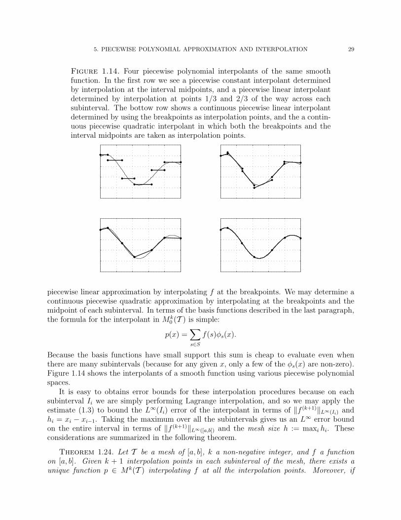
Figure 1.14. Four piecewise polynomial interpolants of the same smoothfunction. In the first row we see a piecewise constant interpolant determinedby interpolation at the interval midpoints, and a piecewise linear interpolantdetermined by interpolation at points 1/3 and 2/3 of the way across eachsubinterval. The bottow row shows a continuous piecewise linear interpolantdetermined by using the breakpoints as interpolation points, and the a contin-uous piecewise quadratic interpolant in which both the breakpoints and theinterval midpoints are taken as interpolation points.
piecewise linear approximation by interpolating f at the breakpoints. We may determine acontinuous piecewise quadratic approximation by interpolating at the breakpoints and themidpoint of each subinterval. In terms of the basis functions described in the last paragraph,the formula for the interpolant in Mk
0 (T ) is simple:
p(x) =∑s∈S
f(s)φs(x).
Because the basis functions have small support this sum is cheap to evaluate even whenthere are many subintervals (because for any given x, only a few of the φs(x) are non-zero).Figure 1.14 shows the interpolants of a smooth function using various piecewise polynomialspaces.
It is easy to obtains error bounds for these interpolation procedures because on eachsubinterval Ii we are simply performing Lagrange interpolation, and so we may apply theestimate (1.3) to bound the L∞(Ii) error of the interpolant in terms of ‖f (k+1)‖L∞(Ii) andhi = xi − xi−1. Taking the maximum over all the subintervals gives us an L∞ error boundon the entire interval in terms of ‖f (k+1)‖L∞([a,b]) and the mesh size h := maxi hi. Theseconsiderations are summarized in the following theorem.
Theorem 1.24. Let T be a mesh of [a, b], k a non-negative integer, and f a functionon [a, b]. Given k + 1 interpolation points in each subinterval of the mesh, there exists aunique function p ∈ Mk(T ) interpolating f at all the interpolation points. Moreover, if

30 1. APPROXIMATION AND INTERPOLATION
Figure 1.15. As the interior mesh points tend to the endpoints, the Lagrangecubic interpolant tends to the Hermite cubic interpolant.
f ∈ C(k+1)([a, b]), then
‖f − p‖L∞([a,b]) ≤1
(k + 1)!‖f (k+1)‖L∞([a,b])h
k+1
where h is the mesh size. Finally, if k > 0 and on each subinterval the interpolation pointsinclude the endpoints, then p ∈Mk
0 (T ).
Remark. The constant 1/(k+1)! can be improved for particular choices of interpolationpoints.
Interpolation by smoother piecewise polynomials (elements of Mks (T ) with s > 0) can
be trickier. For example, it is not evident what set of n + 2 interpolation points to use todetermine an interpolant in M2
1 (T ), nor how to bound the error. The situation for the spaceM3
1 (T ), the space of C1 piecewise cubic polynomials is simpler. Given a C1 function f onan interval [α, β], there is a unique element of p ∈ P3([α, β]) such that
p(α) = f(α), p(β) = f(β), p′(α) = f ′(α), p′(β) = f ′(β).
The cubic p is called the Hermite cubic interpolant to f on [α, β]. It may be obtained as thelimit as ε→ 0 of the Lagrange interpolant using interpolation points α, α + ε, β − ε, and β(see Figure 1.15), and so satisfies
‖f − p‖L∞([α,β]) ≤1
4!‖f (4)‖L∞([α,β]).
Now if we are given the mesh T , then we may define the piecewise Hermite cubic inter-polant p to a C1 function f by insisting that on each subinterval p be the Hermite cubicinterpolant to f . Then p is determined by the interpolation conditions
(1.6) p(xi) = f(xi), p′(xi) = f ′(xi), i = 0, 1, . . . , n.

5. PIECEWISE POLYNOMIAL APPROXIMATION AND INTERPOLATION 31
By construction p ∈M31 (T ). When f ∈ C4([a, b]) we obtain an O(h4) error estimate just as
for the piecewise Lagrange cubic interpolant. We can specify C1 interpolants of higher degreeand order, by supplementing the conditions (1.6) with additional interpolation conditions.Thus to interpolate in Mk
1 (T ), k > 3, we insist that p satisfy (1.6) and as well interpolate f atk− 3 points interior to each subinterval. It is possible to obtain even smoother interpolants(C2, C3, . . . ) using the same idea. But to obtain an interpolant in Cs in this way it isnecessary that the degree k be at least 2s+ 1.
5.1. Cubic splines. The space M32 (T ) of cubic splines has dimension n + 3. It is
therefore reasonable to try to determine an element p of this space by interpolation at thenodes, p(xi) = f(xi), and two additional conditions. There are a number of possible choicesfor the additional conditions. If the values of f ′ are known at the end points a natural choiceis p′(a) = f ′(a) and p′(b) = f ′(b). We shall mostly consider such derivative end conditionshere. If the values of f ′ are not known, one possibility is approximate f ′(a) by r′(a) wherer ∈ P3 agrees with f at xi, i = 0, 1, 2, 3. Another popular possibility is to insist that p′′′
be continuous at x1 and xn−1. This means that p belongs to P3([x0, x2]) and P3([xn−2, xn]).That is, x1 and xn−1 are not true breakpoints or knots. Thus these are called the not-a-knotconditions.
We shall now proceed to proving that there exists a unique cubic spline interpolating fat the breakpoints and f ′ at the end points. With derivative end conditions it is convenientto define x−1 = x0 = a, xn+1 = xn = b and h0 = hn+1 = 0. This often saves us the troubleof writing special formulas at the end points.
Lemma 1.25. Suppose that e is any function in C2([a, b]) for which e(xi) = e′(a) =e′(b) = 0. Then e′′ ⊥M1
0 (T ) in L2([a, b]).
Proof. Let q ∈M10 (T ). Integrating by parts and using the vanishing of the derivatives
at the end points we have ∫ b
a
e′′q dx = −∫ b
a
e′q′ dx.
But, on each subinterval [xi−1, xi], q′ is constant and e vanishes at the end points. Thus∫ xi
xi−1
e′q′ dx = 0.
Theorem 1.26. Given breakpoints x0 < x1 < · · · < xn and values y0, . . . , yn, y′a, y
′b there
exists a unique cubic spline p satisfying p(xi) = yi, p′(a) = y′a, p
′(b) = y′b.
Proof. Since the space of cubic splines has dimension n + 3 and we are given n + 3conditions, it suffices to show that if all the values vanish, then p must vanish. In that case,we can take e = p in the lemma, and, since p′′ ∈M1
0 (T ) we find that p′′ is orthogonal to itself,hence vanishes. Thus p ∈ P1([a, b]). Since it vanishes at a and b, it vanishes identically.
The lemma also is the key to the error analysis of the cubic spline interpolant.
Theorem 1.27. Let f ∈ C2([a, b]) and let p be its cubic spline interpolant with derivativeend conditions. Then p′′ is the best least squares approximation to f ′′ in M1
0 (T ).

32 1. APPROXIMATION AND INTERPOLATION
If we write IM32f for the cubic spline interpolant of f and ΠM1
0g for the L2 projection
(best least squares approximation) of g in M10 , we may summarize the result as
(IM32f)′′ = ΠM1
0f ′′,
or by the commutative diagram
C2([a, b])d2
dx2−−−→ C0([a, b])
IM3
2
y yΠM1
0
M32 (T ) −−−→
d2
dx2
M10 (T )
Proof. We just have to show that the normal equations
〈f ′′ − p′′, q〉 = 0, q ∈M10 (T ),
are satisfied, where 〈 · , · 〉 is the L2([a, b]) inner product. This is exactly the result of thelemma (with e = f − p).
The theorem motivates a digression to study least squares approximation by piecewiselinears. We know that if g ∈ L2([a, b]) there is a unique best approximation p = ΠM1
0g to g
in M10 (T ), namely the L2 projection of g onto M1
0 (T ), determined by the normal equations
〈g − p, q〉 = 0, q ∈M10 (T ).
We now bound the Lebesgue constant of this projection, that is the L∞ operator norm
‖ΠM10‖∞ := sup
f∈C([a,b])‖f‖∞≤1
‖ΠM10f‖L∞ .
Theorem 1.28. ‖ΠM10‖∞ ≤ 3.
Proof. Let φi ∈ M10 (T ) denote the nodal basis function at the breakpoint xi. Then
r = ΠM10f =
∑j αjφj where
n∑j=0
αj〈φj, φi〉 = 〈f, φi〉, i = 0, . . . , n.
Now we can directly compute
〈φj, φj〉 =hj + hj+1
3,
〈φj−1, φj〉 =hj
6,
〈φj, φk〉 = 0, |j − k| ≥ 2,
(recall that by convention h0 = hn+1 = 0). Thus the ith normal equation in this basis is
hiαi−1 + 2(hi + hi+1)αi + hi+1αi+1 = 6〈f, φi〉,where again we define h0 = hn+1 = 0. We remark in passing that the matrix representingthe normal equations in this basis is symmetric, tridiagonal, positive definite, and strictly

5. PIECEWISE POLYNOMIAL APPROXIMATION AND INTERPOLATION 33
diagonally dominant, so easy to solve. (Gaussian elimination without pivoting works in O(n)operations.)
Let α = maxk |αk| = ‖r‖∞. Choose i such that |αi| = α and write the ith equation as
2(hi + hi+1)αi = 6〈f, φi〉 − hiαi−1 − hi+1αi+1.
Taking absolute values we get
2(hi + hi+1)‖r‖∞ ≤ 6|〈f, φi〉|+ hi‖r‖∞ + hi+1‖r‖∞.Now |6〈f, φi〉| ≤ 6‖f‖∞〈1, φi〉 = 3(hi+1 + hi)‖f‖∞ and the result follows.
It follows that ‖f − ΠM10f‖∞ ≤ 4 infq∈M1
0‖f − q‖∞, and, for f ∈ C2, ‖f − ΠM1
0f‖∞ ≤
12h2‖f ′′‖∞.
Returning now to the case of p the cubic spline interpolant of f ∈ C4, we know thatp′′ = ΠM1
0f ′′, so
‖f ′′ − p′′‖∞ ≤1
2h2‖f (4)‖.
This gives a bound on the W 2∞ seminorm. To move down to the L∞ norm, we note that
f − p vanishes at the breakpoints, and hence its piecewise linear interpolant is 0. Applyingthe error estimate for piecewise linear interpolation gives
‖f − p‖∞ ≤1
8h2‖f ′′ − p′′‖∞.
Combining the last two estimates gives us an error bound for cubic spline interpolation:
‖f − p‖∞ ≤1
16h4‖f (4)‖.
The relation (IM32f)′′ = ΠM1
0f ′′ can be used to compute the cubic spline interpolant as
well. We know that
p′′(x) = αj−1xj − xhj
+ αjx− xj−1
hj
, x ∈ [xj−1, xj],
where the αj are determined by the tridiagonal system
hjαj−1 + 2(hj + hj+1)αj + hj+1αj+1 = 6〈f ′′, φj〉.Since integration by parts gives
〈f ′′, φj〉 = (hj + hj+1)f [xj−1, xj, xj+1],
the right-hand side of the tridiagonal system can be written in terms of the data f(xi), f′(a),
f ′(b), so the αi can be computed.Integrating twice we then get
p(x) = αj−1(xj − x)3
6hj
+ αj(x− xj−1)
3
6hj
+ Ajxj − xhj
+Bjx− xj−1
hj
, x ∈ [xj−1, xj].
Finally we may apply the interpolation conditions to find that
Aj = f(xj−1)− αj−1
h2j
6, Bj = f(xj)− αj
h2j
6,
and so we have an explicit formula for p on each subinterval [xj−1, xj].

34 1. APPROXIMATION AND INTERPOLATION
Figure 1.16. A Lagrange basis function for cubic spline interpolation. Thiscubic spline is equal to 1 at the third breakpoint and to 0 at the others,and satisfies zero derivative endpoint conditions. Notice that, although itsmagnitude decreases quickly away from the third breakpoint, it is non-zero onevery subinterval.
While this procedure allows one to efficiently compute the cubic spline interpolant togiven data, it is more complicated than computing a merely continuous piecewise polynomialinterpolant or a Hermite cubic interpolant. This is because, through the linear system whichmust be solved, the cubic spline on each subinterval depends on all the interpolation data,not just the data on the subinterval. Otherwise put, if we define a cubic spline by setting itsvalue equal to one at one of the breakpoints, and its other values and end conditions equalto zero (i.e., a Lagrange basis function for the space of cubic splines, see Figure 1.16), thisfunction will not vanish on any subinterval. (It does, however, tend to decrease quickly awayfrom the breakpoint where it is equal to one, as suggested by the figure.)
6. Piecewise polynomials in more than one dimension
Much of the theory of Lagrange interpolation and best L2 approximation does not extendfrom one to more dimensions. However the theory of continuous piecewise polynomial ap-proximation and interpolation extends rather directly and has many important applications.One of the most important of these is the finite element method for the numerical solutionof partial differential equations which will be studied later in the course.
Here we will consider the case of a plane domain, that is, n = 2, although the extensionto n > 2 is quite similar. Let Ω be a polygon. By a triangulation of Ω we mean a set T ofclosed triangles T with the properties that
(1)⋃
T∈T T = Ω(2) any two distinct elements T1, T2 ∈ T are either disjoint or meet in a common edge
or vertex
The second point means we exclude configurations such as shown in Figure 1.17 from trian-gulations.
Figure 1.18 shows a triangulation of a polygonal domain.As in one-dimension, we write Mk(T ) as the space of functions on Ω whose restriction to
T is a polynomial function of degree at most k. These functions may be discontinuous (andfor our purposes their values on the edges of the triangles are irrelevant). The space Pk(T )of polynomial functions of degree at most k on T has dimension (k + 1)(k + 2)/2 when T isa 2-dimensional domain. Therefore dimMk(T ) = NT(k + 1)(k + 2)/2 where NT where NT
is the number of triangles in the triangulation.

6. PIECEWISE POLYNOMIALS IN MORE THAN ONE DIMENSION 35
Figure 1.17. Inadmissible configurations of triangles for a triangulation.
Figure 1.18. A triangulation and a continuous piecewise linear function.
Of more interest to us is the space
Mk0 (T ) = Mk(T ) ∩ C(Ω),
of continuous piecewise polynomials of degree k with respect to the triangulation T . Anelement of Mk
1 (T ) is plotted along with the mesh in Figure 1.18. Our first task will be todetermine the dimension of this space and exhibit a local basis. First, let k = 1. If weassociate to each vertex of the triangulation a value, then on each triangle we may uniquelydetermine a linear polynomial taking the given values at the vertices. In this way we define apiecewise linear function. The function is continuous. To show this we need only show that iftwo triangles share a common edge, then the linear polynomials determined by interpolationof the vertex values on the two triangles agree on the common edge. But the restrictionof these polynomials to the edge is a linear polynomial in one variable (say in the distancealong the edge from one of the vertices), and they agree at the two endpoints of the edge,so they must agree on the entire edge. In this way we obtain a formula for the dimension ofthe space of piecewise linears with respect to the given triangulation:
dimM10 (T ) = VT ,

36 1. APPROXIMATION AND INTERPOLATION
where VT is the number of vertices in the triangulation. We also obtain a Lagrange basis forM1
0 (T ), a typical element of which is shown in Figure 1.19. For obvious reasons, these arecalled hat functions. Notice that the basis is local: each basis function is zero outside the
Figure 1.19. A typical Lagrange basis function for the space M10 (T ).
union of triangles containing one vertex.Similar considerations allow us to determine the dimension and a local basis for Mk
0 (T )for k > 1. This time we assign values at the vertices and the midpoints of edges. Our firstclaim is that for T a triangle we can determine p ∈ P2(T ) by giving the values at the verticesof T and at the edge midpoints. There is something to prove here, since a priori there mightexist a non-zero quadratic polynomial vanishing at all six of these points. To see that thisdoesn’t happen we notice that the restriction of the polynomial to each edge is a quadraticfunction on the edge which vanishes at three points on the edge. This certainly implies thatthe restriction to each edge vanishes identically. But if a polynomial vanishes on a line, thenit must be divisible by the linear polynomial defining the line. If the three lines through theedges of the triangle are given by li(x) = 0, i = 1, 2, 3, which li ∈ P2(R2), we conclude thatthe polynomial is divisible by the product l1l2l3. Since this product has degree 3 and thepolynomial in question has degree at most 2, the only possibility is that the polynomial isidentically 0.
Thus we can indeed determine an element of M2(T ) by giving arbitrary values at verticesand edge midpoints. To see that the resulting function is in M2
0 (T ) we again observe thaton a common edge to two triangles, the restriction to the edge is fully determined by thevalues at the endpoints and midpoint of the edge. We conclude that
dimM20 (T ) = VT + ET ,
with ET the number of edges of triangles. Figure 1.20 shows a typical basis element associatedwith a vertex and another one associates with and edge midpoint.
Similar considerations apply to continuous piecewise polynomials of any degree. Theappropriate interpolation points for Pk on a single triangle T are shown for degrees 1 through4 in Figure 1.21
6.1. The Bramble–Hilbert Lemma. Our next goals is to obtain error estimates forpiecewise polynomial interpolation in two dimensions. In this section we prove a lemmawhich will be key to obtaining the estimates.

6. PIECEWISE POLYNOMIALS IN MORE THAN ONE DIMENSION 37
Figure 1.20. Two Lagrange basis functions for the space M20 (T ).
Figure 1.21. Interpolation points for Pk(T ), k = 1, 2, 3, 4.
Theorem 1.29 (Bramble–Hilbert Lemma). Let Ω ⊂ RN be a bounded open convex setand let n be a non-negative integer. Then there exists a constant C depending only on Ω andn, such that for 1 ≤ p ≤ ∞,
infp∈Pn(Ω)
‖u− p‖W n+1p (Ω) ≤ C|u|W n+1
p (Ω)
for all u ∈ Cn+1(Ω).
Here, we shall prove the Bramble–Hilbert Lemma in the case of plane domains (N = 2),but essentially the same proof works in any number of dimensions.
We first introduce multi-index notation. Since we are working in R2 a multi-index is just apair α = (α1, α2) of non-negative integers. We write |α| for α1 +α2, D
αu for ∂|α|u/∂xα11 ∂x
α22 ,
xα for xα11 x
α22 , and α! for α1!α2!. With this notation we can state Taylor’s theorem with
remainder for functions of two variables as follows.
Theorem 1.30. Let u be n+1 times continuously differentiable on a neighborhood of theline segment connecting two points x and y in R2. Then
(1.7) u(x) = T ny u(x) +R(x, y),
where
T ny u(x) =
∑|α|≤n
1
α!Dαu(y)(x− y)α
is the Taylor polynomial of degree n for u about y and
R(x, y) =∑
|α|=n+1
n+ 1
α!
∫ 1
0
snDαu(x+ s(y − x)
)(y − x)α ds.

38 1. APPROXIMATION AND INTERPOLATION
Proof. Let F (s) = u(y + s(x− y)). By Taylor’s theorem in one dimension,
F (t) =n∑
m=0
1
m!F (m)(0)tm +
1
n!
∫ t
0
(t− s)nF (n+1)(s) ds.
Taking t = 1 and substituting s 7→ 1− s in the last integral gives the result.
Now we suppose that Ω is a bounded open convex set in R2 and proceed to the proof ofthe Bramble–Hilbert lemma. Translating and dilating we can assume that Ω contains theunit ball B.
Integrating (1.7) over y ∈ B and dividing by π (the area of B), we find that
u(x) = P nu(x) + E(x),
where
P nu(x) =1
π
∫B
T ny u(x) dy
is the averaged Taylor polynomial (note that P nu ∈ Pn(Ω)), and
E(x) =∑
|α|=n+1
n+ 1
πα!
∫R2
∫ 1
0
snDαu(x+ s(y − x)
)χB(y)(y − x)α ds dy.
We have used the characteristic function χB of the unit ball to enable us to write the outerintegral over R2. Next we change variable in the double integral from (s, y) to (t, z) witht = s and z = x+ s(y − x). This gives
E(x) =∑
|α|=n+1
n+ 1
πα!
∫R2
∫ 1
0
t−3Dαu(z)χB
(x+ t−1(z − x)
)(z − x)α dt dz
Now if z /∈ Ω, then also x + t−1(z − x) /∈ Ω, since z lies on the segment joining x to thispoint. Thus χB
(x+ t−1(z − x)
)vanishes whenever z /∈ Ω, and so the outer integral may be
taken over Ω. Rearranging slightly we have
E(x) =∑
|α|=n+1
∫Ω
Dαu(z)
[n+ 1
πα!(z − x)α
∫ 1
0
t−3χB
(x+ t−1(z − x)
)dt
]dz
=∑
|α|=n+1
∫Ω
Dαu(z)Kα(x, z) dz,
where Kα(x, z) is defined to be the term in brackets. We shall prove below:
Lemma 1.31. There exists a constant C depending only on Ω and n such that
Kα(x, z) ≤ C
|x− z|, x, z ∈ Ω.
In particular, ∫Ω
|Kα(x, z)| dx,∫
Ω
|Kα(x, z)| dz ≤ C
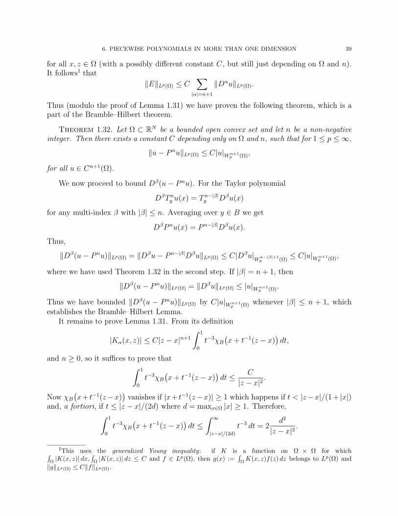
6. PIECEWISE POLYNOMIALS IN MORE THAN ONE DIMENSION 39
for all x, z ∈ Ω (with a possibly different constant C, but still just depending on Ω and n).It follows1 that
‖E‖Lp(Ω) ≤ C∑
|α|=n+1
‖Dαu‖Lp(Ω).
Thus (modulo the proof of Lemma 1.31) we have proven the following theorem, which is apart of the Bramble–Hilbert theorem.
Theorem 1.32. Let Ω ⊂ RN be a bounded open convex set and let n be a non-negativeinteger. Then there exists a constant C depending only on Ω and n, such that for 1 ≤ p ≤ ∞,
‖u− P nu‖Lp(Ω) ≤ C|u|W n+1p (Ω),
for all u ∈ Cn+1(Ω).
We now proceed to bound Dβ(u− P nu). For the Taylor polynomial
DβT ny u(x) = T n−|β|
y Dβu(x)
for any multi-index β with |β| ≤ n. Averaging over y ∈ B we get
DβP nu(x) = P n−|β|Dβu(x).
Thus,
‖Dβ(u− P nu)‖Lp(Ω) = ‖Dβu− P n−|β|Dβu‖Lp(Ω) ≤ C|Dβu|W
n−|β|+1p (Ω)
≤ C|u|W n+1p (Ω),
where we have used Theorem 1.32 in the second step. If |β| = n+ 1, then
‖Dβ(u− P nu)‖Lp(Ω) = ‖Dβu‖Lp(Ω) ≤ |u|W n+1p (Ω).
Thus we have bounded ‖Dβ(u − P nu)‖Lp(Ω) by C|u|W n+1p (Ω) whenever |β| ≤ n + 1, which
establishes the Bramble–Hilbert Lemma.It remains to prove Lemma 1.31. From its definition
|Kα(x, z)| ≤ C|z − x|n+1
∫ 1
0
t−3χB
(x+ t−1(z − x)
)dt,
and n ≥ 0, so it suffices to prove that∫ 1
0
t−3χB
(x+ t−1(z − x)
)dt ≤ C
|z − x|2.
Now χB
(x+ t−1(z−x)
)vanishes if |x+ t−1(z−x)| ≥ 1 which happens if t < |z−x|/(1+ |x|)
and, a fortiori, if t ≤ |z − x|/(2d) where d = maxx∈Ω |x| ≥ 1. Therefore,∫ 1
0
t−3χB
(x+ t−1(z − x)
)dt ≤
∫ ∞
|z−x|/(2d)
t−3 dt = 2d2
|z − x|2.
1This uses the generalized Young inequality : if K is a function on Ω × Ω for which∫Ω|K(x, z)| dx,
∫Ω|K(x, z)| dz ≤ C and f ∈ Lp(Ω), then g(x) :=
∫Ω
K(x, z)f(z) dz belongs to Lp(Ω) and‖g‖Lp(Ω) ≤ C‖f‖Lp(Ω).

40 1. APPROXIMATION AND INTERPOLATION
Remarks. 1. We have given a constructive proof in that we have exhibited a particularp ∈ Pn for which the bound holds. Using functional analysis it is possible to give a muchshorter, but non-constructive, proof. See, for example, [2], Theorem 3.1.1. The proof pre-sented here is along the lines of that in [4]. 2. Usually the result is stated for all u ∈ W n+1
p (Ω)
rather than in Cn+1(Ω). That result follows from this one, using the density of the latterspace in the former. 3. This result became a key tool in approximation theory after the 1970paper of J. Bramble and S. Hilbert [1]. However it can already be found in a much earlierpaper of Deny and Lions [3].
6.2. Error estimates for piecewise polynomial interpolation. Let T be a triangleof diameter hT , and define the linear interpolant
IT : C(T )→ P1(T )
by ITf(v) = f(v) for each vertex v of T . We shall establish the following L∞ error estimate:
Theorem 1.33. There exists an absolute constant C such that
‖f − ITf‖L∞(T ) ≤ Ch2T |f |W 2
∞(T ) for all f ∈ C2(T ).
The proof consists of two main steps. First we prove an estimate of the same form, exceptwithout any indication of how the error depends on the triangle T . Namely:
Theorem 1.34. For each triangle T there exists a constant CT such that
‖f − ITf‖L∞(T ) ≤ CT |f |W 2∞(T ) for all f ∈ C2(T ).
In the second step we shall apply Theorem 1.34 for one particular triangle T and use anaffine map from an arbitrary T to T deduce Theorem 1.33.
Proof of Theorem 1.34. If q ∈ P1(T ), then IT q = q, so f−ITf = (f−q)−IT (f−q).Now clearly ‖ITg‖L∞ ≤ ‖g‖L∞ for all continuous functions g. Applying this with g = f − qgives
‖f − ITf‖L∞ = ‖(f − q)− IT (f − q)‖L∞ ≤ 2‖f − q‖L∞ .Since this is true for all q ∈ P1(T ), by the Bramble–Hilbert lemma (actually only the partof it given in Theorem 1.32), we get
‖f − ITf‖L∞(T ) ≤ CT |f |W 2∞(T ),
for some constant CT , as claimed.
Notice the main ingredients of the proof: first the fact that IT preserve P1 (IT q = q forq ∈ P1(T )); second, boundedness of the interpolant IT (‖ITg‖L∞ ≤ ‖g‖L∞ for all continuousfunctions g); and finally the Bramble–Hilbert lemma.
To go from the estimate of Theorem 1.34, which does not specify dependence of theconstant on T , to that of Theorem 1.33, which shows a dependence of O(h2
T ), we shall applythe former theorem only a single fixed reference triangle, and then use an affine map of thereference triangle onto an arbitrary triangle to deduce the result.
Let T be the reference triangle with vertices v0 = (0, 0), v1 = (1, 0), and v2 = (0, 1), andlet the vertices of T be denoted v0, v1, v2 ∈ R2. There is a unique affine map F taking vi tovi, i = 0, 1, 2, and mapping T one-to-one and onto T . Indeed
Fx = v0 +Bx, B =(v1 − v0 | v2 − v0
),

6. PIECEWISE POLYNOMIALS IN MORE THAN ONE DIMENSION 41
Figure 1.22. Mapping between the reference triangle and an arbitrary triangle.
@@
@@
@@
@@
v0 v1
v2
AAAv0
v1v2
1F
XXXXXXXXXXXXXXXzf R
JJ
JJ
JJJ
f
(the last notation means that B is the 2 × 2 matrix whose columns are the vectors v1 − v0
and v2 − v0). Since the columns of B are both vectors of length at most hT , certainly thefour components bij of B are bounded by hT . Now to any function f on T we may associate
the pulled-back function f on T where
f(x) = f(x) with x = Fx.
I.e., f = f F . See Figure 1.22.Now, the pull-back of the linear interpolant is the linear interpolant of the pull-back:
IT f = ITf . To verify this, it suffices to note that ITfu is a linear polynomial and it agrees
with f at the vertices of T . Moreover, the pull-back operation clearly doesn’t change theL∞ norm. Thus
(1.8) ‖f − ITf‖L∞(T ) = ‖f − IT f‖L∞(T ) ≤ CT |f |W 2∞(T ).
Since T is a fixed triangle, CT is an absolute constant: it doesn’t depend on T . To finish theargument we need to show that
|f |W 2∞(T ) ≤ Ch2
T |f |W 2∞(T ).
This just comes from the chain rule for differentiation. We have
∂f
∂xi(x) =
2∑j=1
∂f
∂xj(x)
∂xj
∂xi=
2∑j=1
bji∂f
∂xj(x).
Differentiating again,
∂2f
∂xi∂xk(x) =
2∑j=1
2∑k=1
bji∂2f
∂xj∂xl(x)blk.
Thus
| ∂2f
∂xi∂xk(x)| ≤ 4h2
T maxj,l| ∂
2f
∂xj∂xl(x)|
and
(1.9) |f |W 2∞(T ) ≤ 4h2
T |f |W 2∞(T ).
Combining (1.8) and (1.9) we complete the proof of Theorem 1.33.

42 1. APPROXIMATION AND INTERPOLATION
We may use the same sort of arguments to obtain estimates in other norms. Firstconsider the Lp norm. In order to obtain Theorem 1.34 we used the boundedness of theinterpolation operator with respect to the L∞ norm: ‖ITg‖L∞ ≤ ‖g‖L∞ . This result is nottrue if we replace L∞ with Lp for p <∞. The difficulty is not with the norm on the left-handside. Indeed ITg lies in the 3-dimensional space P1(T ) and all norms are equivalent on afinite dimensional space. The difficulty is that a continuous function on a triangle may havearbitrarily large vertex values without having a large Lp norm. See Figure 1.23 for the idea inone dimension. Fortunately we really only need boundedness of the interpolant with respect
Figure 1.23. A function with a small Lp norm (solid line), but large inter-polant (dashed line).
to the W 2p norm. That is we need the existence of a constant C such that ‖ITg‖ ≤ C‖g‖W 2
p
for all v ∈ C(T ). (Again, the norm on the left-hand side doesn’t matter in view of theequivalence of norms on the space of polynomials.) Since the interpolant is given in termsof the values of the function at the vertices (ITg(x) =
∑g(vi)li(x) where the li are the hat
functions), the bound on the interpolant reduces to showing that ‖g‖L∞ ≤ C‖g‖W 2p. This is
a special case of the famous Sobolev embedding theorem.
Theorem 1.35 (Sobolev embedding). Let Ω be an n-dimensional domain, p ≥ 1, and man integer greater than n/p. Then there exists a constant C such that
‖g‖L∞ ≤ C‖g‖W mp
for all g ∈ Cm(Ω).
Thus from the Sobolev embedding theorem we know that, in two dimensions, if p > 1,then ‖ITg‖L∞(T ) ≤ CT‖g‖W 2
p, where the constant CT may depend on T , but not on g ∈
C2(T ). We may then argue just as in the proof of Theorem 1.34
‖f − ITf‖Lp = ‖(f − q)− IT (f − q)‖Lp ≤ CT‖f − q‖W 2p≤ C ′
T |f |W 2p,
where we have used polynomial preservation, boundedness, and the Bramble–Hilbert lemmas,respectively.
To obtain a useful Lp error estimate, we apply this result only for the reference triangleT and scale that estimate to an arbitrary triangle. Let |T | denote the area of T . Changingvariables from x to x = Fx, we get∫
T
|(f − ITf)(x)|p dx =|T |2
∫T
|(f − IT f)(x)|p dx ≤ C|T |2
∑|β|=2
∫T
|Dβ f(x)|p dx,

6. PIECEWISE POLYNOMIALS IN MORE THAN ONE DIMENSION 43
where Dβ ranges over the second partial derivatives. Using the chain rule we have
|Dβ f(x)| ≤ Ch2T
∑|γ|=2
|Dγf(x)|
for each β with |β| = 2. Thus∫T
|(f − ITf)(x)|p dx ≤ Ch2pT
|T |2
∑|γ|=2
∫T
|Dγf(x)|p dx = Ch2pT
∑|γ|=2
∫T
|Dγf(x)|p dx.
In other words‖f − ITf‖Lp ≤ Ch2
T |f |W 2p (T ).
Note that the factor of |T |/2, which came from the change of variables x 7→ x disappearedwhen we changed back to the original variable.
Finally we consider estimates of the error in the first derivatives of the interpolants;that is, we bound |f − ITf |W 1
p. As we remarked above, in the boundedness result ‖ITg‖ ≤
CT‖g‖W 2p
(which holds for any p > 1), it does not matter what norm we take on the left-handside. Consequently it is straightforward use the Bramble–Hilbert lemma and show that
(1.10) |f − IT f |W 1p (T ) ≤ C|f |W 2
p (T ).
The next step is to use affine scaling to relate |f − ITf |W 1p (T ) to |f − IT f |W 1
p (T ) and |f |W 2p (T )
to |f |W 2p (T ). We have already made the second relation:
(1.11) |f |W 2p (T ) ≤ Ch2
T |T |−1/p|f |W 2p (T ).
(The factor of h2T comes from applying the chain rule to calculate the second derivatives,
and the factor of |T |−1/p comes from the change of variable in the integral.) To compute|f − ITf |W 1
p (T ) we will again use the chain rule and a change of variables, but this time, since
f = f F−1 with F−1x = −B−1v0 + B−1x, a factor of ‖B−1‖ will appear in our estimate(rather than factors of ‖B‖. Just as we were able to bound ‖B‖ by a geometric quantity,namely by hT = diam(T ), we can bound ‖F−1‖ by a geometric quantity. Let ρT denotethe diameter of the largest disk contained in T (the circumscribed disk). Then any vectorof length ρT is the vector connecting two points in the circumscribed disk, and this vectoris mapped by B−1 to the difference of two points in T , i.e., to a vector of length at most√
2. Thus B−1 maps any vector of length ρT to a vector of length at most√
2, which is theequivalent to saying that ‖B−1‖ ≤
√2/ρT . When we use this result together with the chain
rule and change of variable, we find that
|g|W 1p (T ) ≤
C
ρT
|T |1/p|g|W 1p (T ).
In particular
(1.12) |f − ITf |W 1p (T ) ≤
C
ρT
|T |1/p|f − IT f |W 1p (T ).
Combining (1.12), (1.10), and (1.11), we obtain the estimate
|f − ITf |W 1p (T ) ≤ C
h2T
ρT
|f |W 2p (T ).

44 1. APPROXIMATION AND INTERPOLATION
This argument is almost complete. I need to now define shape regularity and concludea first order estimate. Then state a theorem with all the estimates for piecewise linearinterpolation. Then remark on extension to higher order elements. Perhaps also remark oncase of zero Dirichlet boundary conditions. State final theorem in form to be used in sectionon FEMs.
7. The Fast Fourier Transform
The discrete Fourier transform (DFT) is the linear operator FN : CN → CN given by
(Fny)k =N−1∑j=0
e−2πijk/Nyj, k = 0, 1, 2, . . . , N − 1,
(note that we index the vectors starting from 0). We can use the above formula to define(FNy)k for any k, not just 0 ≤ k < N , but it is an N -periodic sequence. If you recall that
the kth Fourier coefficient of a function f on [0, 1] is defined by f(k) =∫ 1
0f(x)e−2πikx dx,
we see that N−1(FNy)k is just the approximation to f(k) obtained by using the trapezoidalrule with N equal subintervals to compute the integral, expressed in terms of the valuesyj = f(j/N).
Note that application of the DFT is simply multiplication of an N -vector by a particularN × N matrix. This would suggest that N2 multiplications and additions are needed tocompute it. The fast Fourier transform (FFT) is a clever algorithm to compute the DFTmuch more quickly (for large N). Because large DFTs arise in many contexts, the FFTproved to be one of the most important algorithms of the twentieth century. In particular,it has played a tremendous role in signal processing.
The FFT can also be used as a fast means of computing the coefficients of the a trigono-metric interpolating polynomial with equally spaced interpolation points (or for the closelyrelated problem of computing the algebraic polynomial interpolating polynomial at theChebyshev points). In this last section of the chapter we introduce the FFT in that context.
We defined the space Tn of real-valued trigonometric polynomials of degree at most n asthe span of the 2n+ 1 functions 1, cosx, sinx, . . . , cosnx, sinnx. Recall that
Tn = n∑
k=−n
ckeikx | ck ∈ C, c−k = ck .
This space has dimension 2n + 1. However, for reasons that will soon be clear, it is moreconvenient to work with a space of even dimension at this point. Hence we define T ′n as thespan of the 2n functions 1, cos x, sinx, . . . , cosnx, or, equivalently,
T ′n = n∑
k=−n
ckeikx ∈ Tn | c−n = cn = span[1, cosx, sin x, . . . , cosnx].
This space has dimension N = 2n.We now consider the problem of finding a function in T ′n interpolating given data yj at
N equally spaced points xj in [0, 2π]. Since the trigonometric polynomials are 2π-periodic,we include only one of the endpoints, 0, but not 2π, among the interpolation points. Thus

7. THE FAST FOURIER TRANSFORM 45
the interpolation points are xj = 2πj/N , j = 0, . . . , N − 1. The interpolation problem isthus to find coefficients ck ∈ C, k = −n, . . . , n, with cn = c−n, such that
n∑k=−n
cke2πijk/N = yj, j = 0, . . . , N − 1.
(If the yj are real, we may conjugate this equation to find that if (ck) is a solution, then sois (c−k). Since—as we shall see—the solution is unique, we see that the condition ck = c−k
is automatic.)It is possible to write this system of equations in a somewhat more convenient fashion.
If −n ≤ k ≤ −1, we use the identity e2πijk/N = e2πij(k+N)/N . Then n ≤ k +N ≤ N − 1. Inthis way we find
(1.13)n∑
k=−n
cke2πijk/N =
N−1∑k=0
dke2πijk/N
where
dk =
ck, 0 ≤ k < n,
cn + c−n, k = n,
ck−N , n < k < N.
Note that, since cn = c−n, we can recover the ck from the dk.Thus our problem is to find the coefficients dk such that
(1.14)N−1∑k=0
dke2πijk/N = yj.
Once this is done, we can define
(1.15) ck =
dk, 0 ≤ k < n,
dn/2, k = −n or n,
dk+N , −n < k < 0,
to obtain the coefficients of the interpolating trigonometric polynomial.Notice that (1.14) is just an n× n linear system. The matrix is
MN = (e2πijk/N)0≤j,k<N = (ωjk)0≤j,k<N =
1 1 1 . . . 11 ω ω2 . . . ωN−1
1 ω2 ω4 . . . ω2(N−1)
......
.... . .
...
1 ωN−1 ω2(N−1) . . . ω(N−1)2
Thus MN is a Vandermonde matrix based on the powers of ω = ωN = e2πi/N , an Nth rootof unity. Notice the close connection with the DFT: MN is exactly the matrix of the DFT.
The very special form of the matrix MN allows us to write down its inverse explicitly.First note that ω = ω−1. Also, by summing the geometric series, we find
N−1∑k=0
ωjk =
0, j 6≡ 0 (mod N),
N, j ≡ 0 (mod N).

46 1. APPROXIMATION AND INTERPOLATION
Now consider the product MNMN . For 0 ≤ j,m < N , the (j,m) element is
N−1∑k=0
ω−jkωkm =N−1∑k=0
ω(m−j)k = Nδjm.
Thus M−1N = 1
NMN .
To summarize: given a vector of values yj, we take its discrete Fourier transform to geta vector dj, and then rearrange the dj according to (1.15) to get the coefficients cj of thetrigonmetric polynomial of degree at most n interpolating the yj at xj.
In 1965 Cooley and Tukey published a clever way to multiply by FN that exploits itsspecial structure. The resulting algorithm, which exists in many variants, is the FFT. Withit, it is quite practical to compute DFTs of size in the tens of thousands, or even millions.
Let x ∈ RN be given with N = 2n. Let x, x ∈ Rn be the odd and even index elements ofx: xj = x2j, xj = x2j+1. Then
(FNx)k =N−1∑j=0
ω−jkN xj =
n−1∑j=0
ω−2jkN x2j +
n−1∑j=0
ω−(2j+1)kN x2j+1
=n−1∑j=0
ω−jkn xj + ω−k
N
n−1∑j=0
ω−jkn xj
= (Fnx)k + ω−kN (Fnx)k.
This equation shows how to reduce the evaluation of the size N discrete Fourier transformFNx to the two size n discrete Fourier transforms Fnx and Fnx. In matrix terms it shows
FNx
=
Fnx......Fnx
+
1
ω−1N
. . .
ω1−NN
Fnx......Fnx
.
Now if n is itself an even number, then we can reduce each of the discrete Fouriertransforms of size n to two transforms of size n/2, etc. If N is a power of 2, we can continuein this way until we have reduced the work to N transforms of size 1, which of course aretrivial (F1 = 1). Algorithm 1.1 shows, in metacode, an algorithm for computing the FFT inthis case. Notice that the use of recursion makes the algorithm statement quite brief.

7. THE FAST FOURIER TRANSFORM 47
y = FFT(x)input: x = (x0, . . . , xn−1) ∈ Cn where n is a power of 2output: y = Fnx ∈ Cn
if n = 1 theny ← x
elsex← (x0, x2, . . . , xn−2)x← (x1, x3, . . . , xn−1)y ← FFT(x)y ← FFT(x)ω ← e−2πi/n
yk ← yk + ω−kyk, k = 0, 1, . . . , n/2− 1yk ← yk−n/2 + ω−kyk−n/2, k = n/2, n/2 + 1, . . . , n− 1
end if
Algorithm 1.1: Simple FFT.
In fact the code is even briefer when implemented in Matlab,2 as shown in the listingbelow.
function y = simplefft(x)
N = length(x);
if N == 1
y = x;
else
omega = exp(-2*pi*i/N);
ybar = simplefft(x(1:2:N-1));
ytilde = simplefft(x(2:2:N));
y = [ ybar ; ybar ] + omega.^-(0:N-1)’ .* [ ytilde; ytilde ];
end
Algorithm 1.2: Simple FFT implemented in Matlab.
Let us count the amount of work for this algorithm. For simplicity we count only themultiplications and ignore the additions. We also ignore the computation of the powers of ωN
needed in the algorithm. In an efficient implementation, all N powers would be computedonce (via N multiplications). If we let mN be the number of multiplications needed tocompute the action of FN , we have mN = 2mn + N where n = N/2. Also m1 = 0. Thisgives m2k = k2k, i.e., mN = N log2N .
We close with some applications. Figure 1.24 shows a plot of a smooth periodic functionand its derivative on the left. The function was sampled at 16 equally spaced points and its
2Matlab offers an FFT function, fft, which is more sophisticated and also works when N is not a powerof 2.

48 1. APPROXIMATION AND INTERPOLATION
trigonometric polynomial interpolant∑8
k=−8 ckeikx was computed and plotted on the right.
The derivative, computed as∑8
k=−8 ikckeikx, is also shown. This approach to reconstructing
the derivative of a function from its values at a discrete set of points is the basis of spectralmethods for solving differential equations.
Figure 1.24. A trigonometric interpolant and its derivative.
0 1 2 3 4 5 6−1
−0.5
0
0.5
1
0 1 2 3 4 5 6−1
−0.5
0
0.5
1
Of course when N = 16 the efficiency afforded by the FFT is not important. Figure 1.25shows an application involving 1,024 interpolation points, for which the efficiency is signif-icant. On the left are 1024 points (taken from a sound sample of people laughing). In themiddle is the trigonometric polynomial interpolant of the sample values (computed via theFFT), and on the right is a blow-up of the region 2 ≤ x ≤ 2.1 showing that the polynomialdoes indeed interpolate the given values.
Figure 1.25. Trigonometric interpolation at 1,024 points.
0 2 4 6−0.5
0
0.5
0 2 4 6−0.5
0
0.5
2 2.05 2.1−0.5
0
0.5
Exercises
(1) Show that for any 1 ≤ p < q ≤ ∞ the Lp and Lq norms on C(I) are not equivalent.
(2) Let f(x) = ex. a) For p = 1, 2, and ∞ find the best Lp approximation to f in P0(I).b) Same thing but in P1(I).

EXERCISES 49
(3) Prove or disprove: if f ∈ C([−1, 1]) is odd then a best approximation to f by oddpolynomials of degree at most n is a best approximation to f among all polynomials ofdegree n.
(4) Prove or disprove: if f ∈ C([−1, 1]) has mean value zero, then a best approximation tof by polynomials of degree at most n with mean value zero is a best approximation to famong all polynomials of degree n.
(5) State and prove the Jackson theorem in Ck([a, b]) paying attention to the dependence ofthe constant on the interval [a, b].
(6) If f ∈ C(R) and δ > 0 define Rδf ∈ C(R) by
Rδf(x) =1δ
∫ x+δ/2
x−δ/2f(t) dt.
Note that Rδf ∈ C1(R). Prove that ‖f − Rδf‖ ≤ ω(δ), where ω denotes the modulus ofcontinuity of f (i.e., ω(δ) is the supremum of |f(x)−f(y)| over x, y for which |x−y| ≤ δ).
(7) Let f ∈ C2π and let ω denote its modulus of continuity. Using the Jackson theorem inC1
2π and the regularization operator of the previous problem, prove that
infp∈Tn
‖f − p‖∞ ≤ c ω
(1
n + 1
).
Give an explicit expression for c.
(8) Let f ∈ C([−1, 1]) and let ω denote its modulus of continuity. Prove that
infp∈Pn
‖f − p‖∞ ≤ c ω
(1
n + 1
).
Give an explicit expression for c.
(9) Suppose that f ∈ C([−1, 1]) satisfies the Holder condition |f(x) − f(y)| ≤ M |x − y|αwhere M,α > 0. What can you say about the rate of convergence of the best uniformapproximation to f by polynomials of increasing degree?
In the exercises 10–17, which treat divided differences and Newton’s formula forthe interpolating polynomial, we denote by f a real-valued function on an interval,by x0, . . . , xn n + 1 distinct points in J and by pk ∈ Pk the Lagrange interpolatingpolynomial for f at the first k + 1 points x0, . . . , xk.
(10) Prove that pn(x) − pn−1(x) = c(x − x0) · · · (x − xn−1) for some constant c. We use thenotation f [x0, . . . , xn] to denote this constant and call it the nth divided difference of f atthe xi. Use Lagrange’s formula for the interpolating polynomial to derive an expressionfor f [x0, . . . , xn] in terms of xi and f(xi).
(11) Prove that f [x0, . . . , xn] is a symmetric function of its n + 1 arguments.
(12) Prove the recursion relation
f [x0, . . . , xn] =f [x1, . . . , xn]− f [x0, . . . , xn−1]
xn − x0,
where, by convention, f [x] := f(x). (This explains the terminology “divided difference”.)
(13) Give explicit formulas for f [a], f [a, b], f [a, b, c], and f [x, x + h, x + 2h, . . . , x + nh].

50 1. APPROXIMATION AND INTERPOLATION
(14) Prove Newton’s formula for the interpolating polynomial
pn(x) = f [x0] + f [x0, x1](x− x0) + f [x0, x1, x2](x− x0)(x− x1) · · ·+ f [x0, . . . , xn](x− x0) · · · (x− xn−1),
and the error formula
f(x)− pn(x) = f [x0, . . . , xn, x](x− x0) · · · (x− xn).
(15) Prove that if f ∈ Cn(J), then there exists a point ξ in the interior of J such that
f [x0, . . . , xn] =1n!
f (n)(ξ).
(16) Assuming that f ∈ Cn(J), use the recursion defining the divided differences to establishthe Hermite-Gennochi formula
f [x0, . . . , xn] =∫
Sn
f (n)(t0x0 + t1x1 + · · ·+ tnxn) dt,
where
SN =
t = (t1, . . . , tn) ∈ Rn | ti ≥ 0,
n∑1
ti ≤ 1
,
and t0 = 1−∑n
1 ti.
(17) The Hermite-Gennochi formula shows that as a function of n+1 variables the nth divideddifference extends to a function on all of Jn+1 (the arguments need not be distinct). Findsimple closed form expressions for f [a, a], f [a, a, b], and f [a, a, b, b].
For the next 3 problems define Πn : C([−1, 1]) → Pn([−1, 1]) by ‖f − Πnf‖w =infp∈Pn‖f − p‖w, where ‖f‖2w =
∫ 1−1 |f(x)|2(1− x2)−1/2 dx.
(18) Give a formula for Πnf .
(19) Prove that‖f −Πnf‖∞ ≤ c
√n + 1 inf
p∈Pn
‖f − p‖∞
for some constant c. N.B.: This estimate is not sharp. It can be show to hold with√
n + 1replaced by 1 + log(2n + 1), but that is harder to prove.
(20) Prove that if f ∈ Pn+1, then
‖f −Πnf‖∞ = infp∈Pn
‖f − p‖∞,
that is, Πn coincides with best minimax approximation when applied to polynomials ofdegree n + 1.
(21) In proving the convergence of the conjugate gradient method for solving linear systems, akey step is showing that
(1.16) minp∈Pn
p(0)=1
maxx∈[a,b]
|p(x)| = 2(1+√
a/b
1−√
a/b
)n
+(
1−√
a/b
1+√
a/b
)n
for 0 < a < b. In fact, the polynomial for which the minimum is achieved is a scaledChebyshev polynomial:
p(x) = Tn(x)/Tn
(b + a
b− a
), where x =
b + a
2− b− a
2x,

EXERCISES 51
and the right-hand side of (1.16) is just 1/Tn
((b + a)/(b− a)
). Prove all this.
(22) Let f ∈ C1([a, b]). Prove that the cubic spline interpolant with derivative end conditionsminimizes the quantity ‖g′′‖L2([a,b]) among all C2 functions on [a, b] which interpolate f
at the xi and f ′ at a and b. Since the second derivative is a measure of curvature, thissays that in a certain sense the cubic spline interpolant is the straightest, or smoothest,function satisfying the interpolation conditions.
(23) Let x0 < x1 < · · · < xp and suppose that s is a cubic spline defined on all of R withbreakpoints at the xi (only), and for such that s(x) ≡ 0 if x ≤ x0 or x ≥ xp. Provethat if p ≤ 3, then s(x) ≡ 0. In other words, there does not exist a nonzero cubic splinesupported in just 3 intervals.
(24) With the same notation as the previous problem show that that such a nonzero cubicspline s(x) does exist if p = 4. Show that s(x) is determined uniquely up to a constantmultiple. With appropriate normalization s(x) is called the cubic B-spline for the knotsx0, . . . x4.
(25) Give the explicit formula for the cubic B-spline B(x) with knots xi = i, i = 0, . . . , 4,normalized so that
∑B(i) = 1. Draw a plot of this function.
(26) Let ΠN = (ai)∞i=−∞ | ai ∈ C, ai+N = ai denote the space of bi-infinite N -periodiccomplex sequences. If a, b ∈ ΠN we define the convolution c = a ∗ b by
ck =N−1∑j=0
ajbk−j .
Prove that the discrete Fourier transform converts convolution into multiplication: (FNc)k =(FNa)k(FNb)k.
(27) Let p and q be polynomials of degree less than n, where n is a power of 2. Explain howthe coefficients of the product pq can be computed from the coefficients of p and q inO(n log2 n) operations.

Bibliography
1. J. H. Bramble and S. R. Hilbert, Estimation of linear functionals on Sobolev spaces with application toFourier transforms and spline interpolation, SIAM J. Numer. Anal. 7 (1970), 112–124.
2. Philippe G. Ciarlet, The finite element method for elliptic problems, North-Holland, Amsterdam, 1978.3. J. Deny and J. L. Lions, Les espaces du type de Beppo Levi, Ann. Inst. Fourier, Grenoble 5 (1953–54),
305–370 (1955).4. Todd Dupont and Ridgway Scott, Polynomial approximation of functions in Sobolev spaces, Math. Comp.
34 (1980), no. 150, 441–463.5. Theodore J. Rivlin, An introduction to the approximation of functions, Dover Publications Inc., New
York, 1981.6. , Chebyshev polynomials, John Wiley & Sons, New York, 1990.
53


CHAPTER 2
Numerical Quadrature
1. Basic quadrature
The problem is to compute∫ b
af(x) dx given a, b, and an integrable function f on [a, b].
We shall mainly use quadrature rules of the form∫ b
a
f(x) dx ≈n∑
i=0
wif(xi),
with points xi ∈ [a, b] and weights wi ∈ R. More abstractly put, we want to approximate
the functional f 7→∫ b
af by a linear combination of point-evaluation functionals.
Typical examples are:
left endpoint rule:∫ b
af ≈ (b− a)f(a)
midpoint rule:∫ b
af ≈ (b− a)f
((a+ b)/2
)trapezoidal rule:
∫ b
af ≈ b−a
2[f(a) + f(b)]
Simpson’s rule:∫ b
af ≈ b−a
6[f(a) + 4f
((a+ b)/2
)+ f(b)]
2 point Gauss rule:∫ b
af ≈ b−a
2[f((a+ b)/2− (b− a)/(2
√3))
+ f((a+ b)/2 + (b− a)/(2
√3))]
composite midpoint rule (equal subintervals):∫ b
af =
∑ni=1 hf(a− h/2 + ih), h = (b− a)/n
composite midpoint rule (a = x0 < x1 < · · · < xn = b):∫ b
af =
∑ni=1 hif
((xi−1 + xi)/2
), hi = xi − xi−1
For any choice of distinct points xi ∈ [a, b], i = 0, 1, . . . , n there is a natural way to assign
weights wi: let p ∈ Pn interpolate f at the points xi and approximate∫ b
af by
∫ b
ap. Using
Lagrange’s formula p(x) =∑
i f(xi)li(x), with li(x) = Πj 6=i(x − xj)/(xi − xj), we can write
the resulting quadrature rule∫ b
af ≈
∑iwif(xi) where wi =
∫ b
ali(x) dx. Such rules are called
interpolatory quadrature rules. All the rule listed above except the composite midpoint ruleare of this form (the composite rules are based on piecewise polynomial interpolation). Byconstruction an interpolatory quadrature with n+1 points has degree of precision at least n,that is, the rule is exact on all polynomials of degree at most n. For some choices of pointsa higher degree of precision is achieved. For example, Simpson’s rule has degree of precision3 as does the 2 point Gauss rule.
A well-known class of interpolatory quadrature rules are based on using n + 1 equallyspaced points including the end points. These are called the closed Newton-Cotes rules (theword “closed” refers to the fact that the endpoints are included). For n = 1 this is thetrapezoidal rule, for n = 2 it is Simpson’s rule. For n = 3 we get Simpson’s 3/8 rule withweights 1/8, 3/8, 3/8, 1/8 (on an interval of unit length). For n = 4 we get Boole’s rule with
55

56 2. NUMERICAL QUADRATURE
weights 7/90, 32/90, 12/90, 32/90, 7/90. By construction the Newton-Cotes rule with n+ 1points has degree of precision n. But it is also provides the exact value when applied to anyodd power of x− (a+ b)/2 (namely 0) by symmetry. Thus when n is even the Newton-Cotesrule with n+ 1 points has degree of precision n+ 1.
In view of the large Lebesgue constant of high degree interpolation with equally spacedpoints, it is not suprising that the Newton-Cotes rules are not very good for n large. Startingwith n = 8 some of the weights are negative, and for larger n the coefficients become verylarge and oscillatory (they sum to one). As a result the formulas are very sensitive to errorsin f and difficult to evaluate in finite precision (cancellation).
For interpolatory quadrature rule we can deduce the error from the error formula forLagrange interpolation. As an example consider the trapezoidal rule on the unit interval[0, 1], which is based on Lagrange interpolation at the points 0 and 1. Denoting by p theinterpolant, we have f(x)− p(x) = f [x, 0, 1]x(x− 1), so the error in the trapezoidal rule is
(2.1) err =
∫ 1
0
f −∫ 1
0
p =
∫ 1
0
f [x, 0, 1]x(x− 1) dx.
We now recall the integral mean value theorem: if u ∈ C([a, b]) and w is an integrable (butnot necessarily continuous) function on [a, b] which doesn’t change sign, then∫ b
a
u(x)w(x) dx = u(η)
∫ b
a
w(x) dx
for some η ∈ (a, b). Applying this to the integral on the right-hand side of (2.1) withu(x) = f [x, 0, 1] and w(x) = x(x− 1) we find that∫ 1
0
f −∫ 1
0
p = −1
6f [η, 0, 1]
for some η ∈ (0, 1), and hence, if f ∈ C2([0, 1]),
err = f [η, 0, 1]
∫ 1
0
x(x− 1) dx = − 1
12f ′′(ξ)
for some ξ ∈ (0, 1).Next we scale this result to an arbitrary interval [α, β]. If f ∈ C2([α, β]), we define
f(x) = f(x) where x = α+ (β − α)x. Then∫ β
α
f − β − α2
[f(α) + f(β)] = (β − α)
∫ 1
0
f − 1
2[f(0) + f(1)]
= − 1
12(β − α)f ′′(ξ) = − 1
12(β − α)3f ′′(ξ),
for some ξ ∈ (α, β).Now consider the composite trapezoidal rule using n equal subintervals of size h = (b−
a)/n. Applying the above result on each subinterval and summing we get∫ b
a
f − h[12f(a) +
n−1∑i=1
f(a+ ih) +1
2f(b)] = − 1
12h3
n∑i=1
f ′′(ξi) = − 1
12(b− a)h2f ′′(ξ).

2. THE PEANO KERNEL THEOREM 57
Here ξi ∈ (a+ (i− 1)h, a+ ih) and we have used the fact that∑
i f′′(ξi) = nf ′′(ξ) for some
ξ ∈ (a, b) (again a consequence of the intermediate value theorem). This is an exact formula,not just a bound, for the error. It implies the bound |err| ≤ (b− a)h2/12‖f ′′‖L∞ .
Now consider the composite trapezoidal rule with unequal subintervals determined by apartition a = x0 < . . . xn = b. With hi = xi − xi−1, h = maxi hi, we have∣∣∣∣∣∫ b
a
f −n∑
i=0
hi
2[f(xi−1) + f(xi)]
∣∣∣∣∣ =
∣∣∣∣∣− 1
12
n∑i=1
h3i f
′′(ξi)
∣∣∣∣∣≤ 1
12h2∑
hi‖f ′′‖L∞ =1
12(b− a)h2‖f ′′‖L∞ ,
and we see that this bound is sharp since equality must hold if f ′′ is constant.Note that we get the same bound |err| ≤ (b− a)h2/12‖f ′′‖L∞ for an unequal spacing of
points as for uniform spacing. Of course this bound doesn’t show any particular advantageto choosing a nonuniform spacing. For that we would have to consider more carefully thesum
∑i h
3i f
′′(ξi). If we adjust the spacing so that hi is smaller where |f ′′| is larger we candecrease the error.
If we try to apply the same arguments to the midpoint rule we come across one difference.For the midpoint rule on [0, 1] the interpolant is simply the constant value f(1/2), and sowe get, instead of (2.1),
err =
∫ 1
0
f − f(1/2) =
∫ 1
0
f [x, 1/2](x− 1/2) dx.
However now the kernel x− 1/2 changes sign on [0, 1] and so we cannot continue using theintegral mean value theorem as before.
A simple approach for the midpoint rule is to use Taylor’s theorem. Assuming thatf ∈ C2([0, 1]) we have
f(x) = f(1/2) + f ′(1/2)(x− 1/2) +1
2f ′′(ξx)(x− 1/2)2, x ∈ (0, 1)
where ξx ∈ (0, 1) depends continuously on x. Integrating over x ∈ (0, 1) we get
(2.2)
∫ 1
0
f − f(1/2) =1
2
∫ 1
0
f ′′(ξx)(x− 1/2)2 dx =1
24f ′′(ξ),
for some ξ ∈ (0, 1). Note that term involving x − 1/2 integrated to zero and we were ableto use the integral mean value theorem in the last term because (x − 1/2)2 is everywherenon-negative. Once we have the expression (2.2) for the error in the simple midpoint ruleon the unit interval, we can scale to an arbitary interval and add up over subintervals justas for the trapezoidal rule. We find that the error is bounded by (1/24)(b − a)h2‖f ′′‖L∞ ,exactly 1/2 times the bound we got for the trapezoidal rule.
2. The Peano Kernel Theorem
In the last section we derived expressions for the error in the simple trapezoidal andmidpoint rules on the unit interval, and then scaled and summed to get bounds for the errorin the composite rules. In this section we describe an approach that can be used to giveeasily manipulated expressions for the error in any quadrature rule.

58 2. NUMERICAL QUADRATURE
Define two linear functionals on C([a, b]) by the integral and by the quadrature rule:
If =∫ b
af , Jf =
∑ni=0wif(xi). If the degree of the precision of the quadrature rule is d,
then the error functional Ef := If−Jf vanishes on Pd. From this fact alone we can derive avery useful expression for the error. The approach is very much like the one we used to deriveinterpolation error estimates on triangles in Chapter 1.6.2. In deriving the Bramble–Hilbertlemma we represented an arbitrary function in Ck as the sum of a polynomial of degree atmost k (the averaged Taylor polynomial), and an integral of the k + 1st derivatives of thefunction times suitable kernel functions. In one dimension the story is simpler, because wecan use the ordinary Taylor theorem with remainder, without the averaging.
Let 0 ≤ k ≤ d be an integer and suppose that f ∈ Ck+1([a, b]). Then, by Taylor’stheorem,
f(x) = p(x) +1
k!
∫ x
a
f (k+1)(t)(x− t)k dt,
with p ∈ Pk the Taylor polynomial for f about x = a. Now let us write xn+ = xn for
x > 0, 0 otherwise. We can then express the remainder in Taylor’s theorem as r(x) =1k!
∫ b
af (k+1)(t)(x − t)k
+ dt. Since f = p + r and Ep = 0, we have Ef = Er. This gives thePeano Kernel representation of the error:
Ef =
∫ b
a
f (k+1)(t)K(t) dt
where K(t) = Ex[(x− t)k+]/k!. The key point is that when the linear functional E vanishes
on Pk, we can express Ef as the integral of f (k+1)(t) times an explicit function K(t). Thefunction K(t) is called the Peano kernel of the error. To establish this result we requiredonly that E be a linear functional which vanishes on polynomials of degree k and be of aform that commutes with integration. So it can be used for bounding errors in other contextsthan numerical integration. Note also that if E vanishes on Pk, it also vanishes on Pk−1,Pk−2, etc. So we have k different Peano kernel representations of the error, which express itas integral involving f ′, f ′′, . . . , f (k+1). We refer to the corresponding Peano kernels as thefirst derivative Peano kernel, the second derivative Peano kernel, etc.
As an example of the application of the Peano kernel error representation, we reanalyzethe midpoint rule from using it. Again, we consider first the unit interval and so define
Ef =
∫ 1
0
f − f(1/2).
The degree of precision is 1, so we have two error representations. If f ∈ C2, we haveEf =
∫ 1
0f ′′(t)K(t) dt with
K(t) =
∫ 1
0
(x− t)+ dx− (1/2− t)+ =
t2/2, 0 ≤ t ≤ 1/2,
(1− t)2/2, 1/2 ≤ t ≤ 1
This is the second derivative Peano kernel for the midpoint rule on [0, 1], and is plotted onthe left of Figure 2.1, which also shows the second derivative Peano kernel for the trapezoidalrule and Simpson’s rule. Note that the midpoint rule Peano kernel satisfies K ≥ 0 on [0, 1],‖K‖L∞ = 1/8, ‖K‖L1 = 1/24.

2. THE PEANO KERNEL THEOREM 59
Figure 2.1. The second derivative Peano kernels for the midpoint rule, thetrapezoidal rule, and Simpson’s rule. on [0, 1].
0 0.5 1−0.2
0
0.2
0 0.5 1−0.2
0
0.2
0 0.5 1−0.2
0
0.2
Next scale to an arbitrary interval [α, β] to find the Peano kernel in that case. Todistinguish between the Peano kernel for the midpoint rule on [0, 1] and the Peano kernel forthe midpoint rule on [α, β], at this point we will write K[0,1] and K[α,β] for the latter. With
t = (t− α)/(β − α) we have∫ β
α
f(x) dx−(β−α)f(α+ β
2
)= (β−α)
[∫ 1
0
f(x) dx− f(1/2)
]= (β−α)
∫ 1
0
f ′′(t)K[0,1](t) dt
= (β − α)3
∫ 1
0
f ′′(t)K[0,1](t) dt = (β − α)2
∫ β
α
f ′′(t)K[0,1](t) dt =
∫ β
α
f ′′(t)K[α,β](t) dt,
where
K[α,β](t) = (β − α)2K[0,1](t) =
(t− α)2/2, α ≤ t ≤ α+β
2,
(β − t)2/2, α+β2≤ t ≤ β.
For the Peano kernel on [α, β] we have K[α,β] ≥ 0 and ‖K[α,β]‖L1 = (β − α)3/24.As an immediate consequences we obtain:
Ef =(β − α)3
24f ′′(ξ) for some ξ ∈ (α, β), |Ef | ≤ (β − α)3
24‖f ′′‖L∞ ,
Note that the first result is an exact expression for the error and used the fact that K[α,β] isof one sign, while the only property of K[α,β] entering the error bound are its L1 norm.
Now consider the composite midpoint rule arising from a partition a = x0 < · · · < xn = b.Once again we have a Peano kernel error representation,
(2.3)
∫ b
a
f −n∑
i=1
hif(xi−1 + xi
2
)=
∫ b
a
f ′′(t)K(t) dt,
where now
(2.4) K(t) =
(t− xi−1)
2/2, xi−1 ≤ t ≤ (xi−1 + xi)/2,
(xi − t)2/2, (xi−1 + xi)/2 ≤ t ≤ xi,
i = 1, . . . , n. Note that again K ≥ 0 and now ‖K‖L∞ = supi h2i /8 = h2/8. We thus obtain
Ef =1
24
(∑i
h3i
)f ′′(ξ) for some ξ ∈ (a, b), |Ef | ≤ (b− a)h2
24‖f ′′‖L∞ .(2.5)
Thus if f ∈ C2([a, b]), the composite midpoint rule converges as the second power of themaximal subinterval size.
60 2. NUMERICAL QUADRATURE
We can also use the Peano kernel theorem to represent the error as the integral of thefirst derivative of the integrand times the kernel K0(t) = E[( · − t)+0]. In fact, rather thancompute this, let us derive the final (composite rule) representation by integrating by partsin (2.3). Writing K1 for the kernel given by (2.4) we have∫ b
a
f −n∑
i=1
hif(xi−1 + xi
2
)=
∫ b
a
f ′′(t)K1(t) dt = −∫ b
a
f ′(t)K ′1(t) dt,
so
K0(t) = −K ′1(t) =
xi−1 − t, xi−1 ≤ t ≤ (xi−1 + xi)/2,
xi − t, (xi−1 + xi)/2 ≤ t ≤ xi.
Note that in this case the kernel does not have constant sign. The L1 norm is easily bounded:‖K0‖L1 =
∑h2
i /4 ≤ (b − a)h/4. We thus get another estimate for the composite midpointrule, valuable especially for f which is not in C2([a, b]):
|Ef | ≤ (b− a)h4
‖f ′‖L∞ .
Remark. We have bounded the Peano kernels in L1 in order to obtain an error boundinvolving the L∞ norm of a derivative of the solution. It is also possible to use an Lp boundfor the Peano kernel (p > 1) in order to obtain a bound in terms of the Lq (q = p/(p−1) <∞)norm of a derivative of the solution. This is preferable in cases were the derivative is singularor nearly so.
3. Richardson Extrapolation
Let J1 be a quadrature rule on the unit interval with degree of precision p. That isE1f := If − J1f = 0 for f ∈ Pp, but not, in general for f ∈ Pp+1. We can then write
E1f =∫ 1
0fp+1(t)K1(t) dt. Let c1 =
∫ 1
0K1. Note that c1 6= 0, since that would imply degree
of precision at least p+ 1.Now let J2 be another quadrature of the same degree of precision, and let c2 denote the
corresponding constant. Assume that c2 6= c1. Then it is possible to find a linear combinationJ = α1J1+α2J2 of the rules, which is itself a quadrature rule with degree of precision greaterthan p. Indeed, define the αi by the equations α1 +α2 = 1 and α1c1 +α2c2 = 0. With thesevalues, suppose f ∈ Pp+1 so f (p+1) is constant. Then
If − (α1J1f + α2J2f) = α1(If − J1f) + α2(If − J2f) = α1c1f(p+1) + α2c2f
(p+1) = 0.
That is, Jf := α1J1f + α2J2f is a new quadrature rule of higher precision.As an example, let J1f = [f(0) + f(1)]/2 be the trapezoidal rule and J2f = f(1/2)
the midpoint rule. Then we have c1 = −1/12, c2 = 1/24, so α1 = 1/3, α2 = 2/3, andJf = f(0)/6+2/3f(1/2)+f(1)/6, which is precisely Simpson’s rule. Note that the new rulehas degree of precision at least 2 by construction, but actually 3, since, as usual, a symmetricrule integrates odd powers exactly.
One common way to apply Richardson’s extrapolation is with a quadrature rule andthe same rule applied in composite form with two subintervals of equal length. Thus, forexample, we could combine the trapezoidal rule J1f with J2f := [f(0) + 2f(1/2) + f(1)]/4.For this purpose it is not even necessary to know the error constant c1 for J1, but onlythe fact that the degree of precision of the rule is 1. When we apply the composite form

4. ASYMPTOTIC ERROR EXPANSIONS 61
this means we bring in a factor of the second power of the subinterval size, i.e., a factorof 1/4, so c2 = c1/4. Thus α1 = −1/3 and α2 = 4/3, and the new rule turns out to beSimpson’s rule again. The general pattern is that if J1 is a rule with degree of precision p,and J2 is the same rule applied with two subintervals, then the constants ci are in the ratio2p+1 : 1 so α1 = −1/(2p+1 − 1), α2 = 2p+1/(2p+1 − 1). As a second example, suppose thatJ1f = [f(0) + 3f(1/3) + 3f(2/3) + f(1)]/8 is Simpson’s 3/8 rule, so p = 3. Then
Jf = − 1
15[f(0) + 3f(1/3) + 3f(2/3) + f(1)]/8
+16
15[f(0) + 3f(1/6) + 3f(1/3) + 2f(1/2) + 3f(2/3) + 3f(6/6) + f(1)]/16
=1
120[7f(0) + 24f(1/6) + 21f(1/3) + 16f(1/2) + 21f(2/3) + 24f(5/6) + 7f(1)].
The result 7 point rule has degree of precision 5 (so does not coincide with the 7 point closedNewton-Cotes rule, which has degree of precision 7).
4. Asymptotic error expansions
Consider again the error in the trapezoidal rule
Ef = If − Jf =
∫ 1
0
f − f(0) + f(1)
2.
We have Ef =∫ 1
0Kf ′′ where
∫ 1
0K = −1/12. Now if f ∈ P2 then f ′′ is constant, so∫ 1
0(K + 1/12)f ′′ = 0. Thus
Ef =
∫ 1
0
Kf ′′ = − 1
12
∫ 1
0
f ′′ +
∫ 1
0
(K + 1/12)f ′′ =1
12[f ′(0)− f ′(1)] + 0.
In other words, if the quadrature rule
Jf =f(0) + f(1)
2+f ′(0)− f ′(1)
12,
(known as the trapezoidal rule with endpoint corrections), has degree of precision at least2. By symmetry, again, we see it has degree of precision 3. The use of derivative values inthe quadrature rule is unusual, but we still get a linear functional to which we can applythe Peano kernel theorem, and hence this rule will be fourth order accurate when applied incomposite form, that is, the error will be bounded by a multiple of h4‖f (4)‖L∞ where h is themaximum subinterval size. The fact that the derivative values enter only as the difference(not the sum!) at the endpoints leads to a big simplification for the composite rule withequal subintervals. If h = (b − a)/n, xi = a + ih, and Jhf denotes the usual compositetrapezoidal rule, then the composite trapezoidal rule with endpoint corrections is simply∫ b
a
f ≈ Jhf = Jhf + h2f′(a)− f ′(b)
12.
Since this rule is fourth order accurate, we have identified the leading term of an asymptoticexpansion of the error is the (ordinary) composite trapezoidal rule as a function of h. We
62 2. NUMERICAL QUADRATURE
knew before that Eh =∫ b
af − Jhf = O(h2). We know now that
Ehf = c2h2 +O(h4),
where c2 is precisely [f ′(b)− f ′(a)]/12.With careful analysis we can determine the entire asymptotic expansion of Ehf . To do
this, we need to introduce the Bernoulli polynomials Bn(x). There are many ways to definethe Bernoulli polynomials. We use:
• B0(x) = 1• B1(x) = x− 1/2• B′
n(x) = nBn−1(x), n = 2, 3, . . .• Bn(0) = Bn(1) = 0 for n = 3, 5, 7, . . .
This clearly uniquely determines all the odd-indexed polynomials as the solution of theboundary value problem
B′′n(x) = n(n− 1)Bn−2(x), Bn(0) = Bn(1) = 0, n = 3, 5, . . . ,
and then the equation nBn−1(x) = B′n(x) determines the even-indexed Bernoulli polynomi-
als. Note that Bn(x) is a monic polynomial of degree n and is an odd or even function ofx− 1/2 according to whether n is odd or even.
B0(x) = 1,(2.6)
B1(x) = x− 1
2,(2.7)
B2(x) = (x− 1
2)2 − 1
12= x2 − x+
1
6,(2.8)
B3(x) = (x− 1
2)3 − 1
4(x− 1
2) = x3 − 3
2x+
1
2x,(2.9)
B4(x) = (x− 1
2)4 − 1
2(x− 1
2)2 +
7
48(x− 1
2) = x4 − 2x3 + x2 − 1
30.(2.10)
The Bernoulli numbers are defined by Bk = Bk(0). Thus B1 = −1/2 and Bk = 0 fork = 3, 5, 7 . . .. B0 = 1, B2 = 1/6, B4 = −1/30, B6 = 1/42.
Remark. Euler gave a generating function for the Bernoulli polynomials:
tetx
et − 1=
∞∑n=0
Bn(x)tn
n!,
and this is often used to define them. Setting x = 0 we get a generating function for theBernoulli numbers:
t
et − 1=
∞∑n=0
Bntn
n!.
Now we apply the Bernoulli polynomials to expand∫ 1
0f in terms of the values of f and
its derivatives at 0 and 1. This will give the trapezoidal rule, the endpoint corrections, and

4. ASYMPTOTIC ERROR EXPANSIONS 63
then higher endpoint corrections. The derivation is simply repeated integration by parts:∫ 1
0
f(x) dx =
∫ 1
0
f(x)B0(x) dx =
∫ 1
0
f(x)B′1(x) dx
=1
2[f(0) + f(1)]−
∫ 1
0
f ′(x)B1(x) dx
=1
2[f(0) + f(1)]− 1
2
∫ 1
0
f ′(x)B′2(x) dx
=1
2[f(0) + f(1)] +
B2
2[f ′(0)− f ′(1)] +
1
2
∫ 1
0
f ′′(x)B2(x) dx.
Now1
2
∫ 1
0
f ′′(x)B2(x) dx =1
4!
∫ 1
0
f ′′(x)B′′4 (x) dx,
so integrating by parts two more times gets us to∫ 1
0
f(x) dx
=1
2[f(0) + f(1)] +
B2
2[f ′(0)− f ′(1)] +
B4
4![f ′′′(0)− f ′′′(1)] +
1
4!
∫ 1
0
f (4)(x)B4(x) dx.
Continuing this argument (formally, using induction) we prove:
Theorem 2.1. Let m be a positive integer, f ∈ C2m([0, 1]). Then∫ 1
0
f(x) dx
=1
2[f(0) + f(1)] +
m∑k=1
B2k
(2k)![f (2k−1)(0)− f (2k−1)(1)] +
1
(2m)!
∫ 1
0
f (2m)(x)B2m(x) dx.
This theorem gives the formula for the trapezoidal rule with m endpoint corrections andshows that it has degree of precision at least 2m−1, and exhibits the Peano kernel. However∫ 1
0B2m(x) dx = 2m[B2m−1(1)−B2m−1(0)] = 0, so the degree of precision is at least 2m, and
by parity, actually 2m + 1. To derive the Peano kernel error representation in terms of the2m + 2 derivative, replace m by m + 1 in the expansion and combine the final term of thesum with the integral to get∫ 1
0
f(x) dx =1
2[f(0) + f(1)] +
m∑k=1
B2k
(2k)![f (2k−1)(0)− f (2k−1)(1)] +Rm,
where
Rm =B2m+2
(2m+ 2)![f (2m+1)(0)− f (2m+1)(1)] +
1
(2m+ 2)!
∫ 1
0
f (2m+2)(x)B2m+2(x) dx
=1
(2m+ 2)!
∫ 1
0
f (2m+2)(x)[B2m+2(x)−B2m+2] dx.

64 2. NUMERICAL QUADRATURE
Thus we see that the trapezoidal rule with m end corrections has degree of precision 2m+ 1and the Peano kernel for the 2m+ 2nd derivative is [B2m+2(x)−B2m+2(0)]/(2m+ 2)!. Notethat this kernel does not change sign (since the even indexed Bernoulli polynomials aremonotonic on [0, 1/2] and even), and that its integral is −B2m+2/(2m + 2)! (since the evenindexed Bernoulli polynomials have mean value zero). Thus we have the following theorem.
Theorem 2.2. Let m be a positive integer, f ∈ C2m+2([0, 1]). Then∫ 1
0
f(x) dx =1
2[f(0) + f(1)] +
m∑k=1
B2k
(2k)![f (2k−1)(0)− f (2k−1)(1)] +Rm
where
Rm =1
(2m+ 2)!
∫ 1
0
f (2m+2)(x)[B2m+2(x)−B2m+2] dx = − B2m+2
(2m+ 2)!f (2m+2)(ξ)
for some ξ ∈ (0, 1).
From this we easily get a result for the composite trapezoidal rule.
Corollary 2.3. Let m and n be positive integers and f ∈ C2m+2([a, b]) for some a < b.Set h = (b− a)/n, xi = a+ ih. Then∫ b
a
f(x) dx =h
2[f(a) + 2
n−1∑i=1
f(xi) + f(b)] +m∑
k=1
B2k
(2k)!h2k[f (2k−1)(a)− f (2k−1)(b)] +Rm
where
Rm = − B2m+2
(2m+ 2)!(b− a)h2m+2f (2m+2)(ξ),
for some ξ ∈ (a, b).
For smooth periodic functions integrated over a period, the endpoint corrections disap-pear and the ordinary trapezoidal rule (with constant subintervals) is O(hp) for any p:
Corollary 2.4. Let m and n be positive integers and f ∈ C2m+2(R) is periodic withperiod T . Let a ∈ R, b = a+ T , h = T/n, xi = a+ ih. Then∫ b
a
f(x) dx = h
n−1∑i=0
f(xi) +Rm
where
Rm = − B2m+2
(2m+ 2)!(b− a)h2m+2f (2m+2)(ξ),
for some ξ ∈ (a, b).
In fact, if f is real-analytic and periodic, then the convergence of the trapezoidal rule isexponential. We can deduce this from our previous analysis of the approximation of periodicanalytic functions by trigonometric polynomials (and so we don’t need the Euler-Maclaurinexpansion for this). Assume for simplicity that the period is 2π and recall that we provedthat for such f there exist positive constants C and δ for which infq∈Tn‖f − q‖L∞ ≤ Ce−δn.
Now if q(x) = eimx, m 6= 0, then∫ 2π
0q = 0 and
∑n−1k=0 q(k/n) = 0 for all n which are not
divisors on m. In particular, if we write En for the error operator for the trapezoidal rule

5. ROMBERG INTEGRATION 65
with n equal subintervals, Enq = 0 for all q ∈ Tn−1. Note also that |Eng| ≤ 2‖g‖L∞ for anycontinuous g. Thus
|Enf | = infq∈Tn−1
|En(f − q)| ≤ 2 infq∈Tn−1
‖f − q‖L∞ ≤ 2Ce−δ(n−1) = C ′e−δn.
Theorem 2.5. Let f be real-analytic and T -periodic, b = a+T . Then there exist positiveconstants δ and C such that∣∣∣∣∣
∫ b
a
f − T
n
n−1∑k=0
f(a+ kT/n)
∣∣∣∣∣ ≤ Ce−δn.
5. Romberg Integration
Suppose we compute the trapezoidal rule approximation to I =∫ b
af using equal subin-
tervals of size h, and compute it again using twice as many subintervals of size h/2. Call theresulting approximations Thf and Th/2f , respectively. Then, assuming f is smooth, we have
I = Thf + c1h2 + c2h
4 + · · · ,
I = Th/2f +1
4c1h
2 +1
16c2h
4 + · · · .
Here the ci are independent of h (c1 = [f ′(a)− f ′(b)]/12,. . . ). We may then use Richardsonextrapolation to obtain an O(h4) approximation to I: with T 1
h/2 = (4Th/2f − Th)/3 we have
I = T 1h/2 + c12h
4 + c13h6 + · · ·
for some numbers c21 independent of h. Of course we know that the fourth order rule T 1 isjust Simpson’s rule.
If we also compute Th/4f as well, that we can combine similarly it with Th/2f to obtainT 1
h/4f , and for which the leading term of the error will be (c12/16)h4. We can then combine
T 1h/2f and T 1
h/4 by Richardson extrapolation to obtain a sixth order rule: T 2h/4 = (16T 1
h/4 −T 1
h/2)/15. In fact, using the same set of functional evaluations we need to compute the 2ndorder rule Th/2mf we can obtain a 2mth order rule Tm
h/2mf . The following diagram shows theorder of computation.
Thf
Th/2f → T 1h/2f
Th/4f → T 1
h/4 → T 2h/4f
......
.... . .
Th/2mf → T 1h/2mf → T 2
h/2mf · · · Tmh/2mf
This systematic use of Richardson extrapolation to obtain the highest possible order fromthe given point evaluations is called Romberg Integration. The computation of the finalapproximation Tm
h/2mf is very cheap once the first column has been generated (namely once
f has been evaluated at all the necessary points), but it often gives a drastic improvementin accuracy.

66 2. NUMERICAL QUADRATURE
This diagram is reminiscent of a divided difference table for computing an interpolatingpolynomial. In fact, there is a direct connection. Let us denote by T (h) the trapezoidal ruleapproximation to I using equal subintervals of size h. (Of course T (h) is only defined whenh = (b− a)/n for some positive integer n.) The limh→0 T (h) = I. If we have computed T (h)for m+ 1 distinct positive values of h, h0, . . . , hm, then a natural way to estimate I = T (0)is to compute the Lagrange interpolating polynomial determined by these m+ 1 values of hand T (h) and estimate I by the value of the interpolating polynomial at 0. Actually, sincewe know from the Euler-Maclaurin expansion that T (h) has an asymptotic expansion inpowers of h2, we shall use a polynomial in h2: P (h) = Q(h2) =
∑mk=0 akh
2k. The polynomialQ ∈ Pm is determined by the conditions Q(h2
i ) = Thif . For example, if we have computed
Th0f and Th1f , then
Q(x) = Th0f +Th1f − Th0f
h21 − h2
0
(x− h20),
so
I ≈ Q(0) =h2
0Th1f − h21Th0f
h21 − h2
0
,
In particular, if h1 = h0/2, then
I ≈ Q(0) =4Th1f − Th0f
3,
and we see that this procedure reduces to Richardson extrapolation (this in fact explainsthe use of the word “extrapolation”). In general, if we compute Thi
f for i = 0, . . . ,m withhi = h0/2
i, and then compute the polynomial Q ∈ Pm determined by Q(h2i ) = Thi
f , it canbe checked that Q(0) is exactly Tm
h0/2mf , the result of Romberg integration. For this reason,Romberg integration is sometimes called extrapolation to the limit. This analysis also showsthat it is not necessary that the hi = h0/2
i. We could use another sequence of values of hi
as well. Of course the sequence h0/2i is convenient, because it means that all the function
evaluation needed to compute Thmf are sufficient to compute all the Thif .
Remark. Note that the idea of extrapolation to the limit applies not only to error inquadrature, but whenever we know that the error has an asymptotic expansion in powers ofa parameter h. We have assumed the expansion is a sum of even powers, but this can begeneralized to allow an expansion in an arbitrary sequence of (known) powers.
6. Gaussian Quadrature
Consider an ordinary quadrature rule with n points x1 < x2 < · · · < xn and weightsw1, w2, . . . , wn: ∫ b
a
f(x) dx ≈n∑
i=1
wif(xi).
What is the maximal possible degree of precision? For example, it’s obvious that if n = 1,the maximal possible degree of precision is 1, which is achieved by the midpoint rule. Forany number of points, an upper bound is immediate:
Theorem 2.6. The degree of precision of an n-point rule is < 2n.

6. GAUSSIAN QUADRATURE 67
Proof. The function f(x) =∏n
i=1(x− xi)2 is a polynomial of degree 2n. Clearly
∫f >
0 =∑wif(xi).
We shall show that the maximum possible degree of precision 2n − 1 is achieved by aunique n-point rule. Without loss of generality, we may restrict to the interval [a, b] = [−1, 1].Our chief tool will be the Legendre polynomials Pn(x). Recall that degPn = n and Pn isL2([−1, 1])-orthogonal to Pn−1. Let x1 < · · · < xn denote the roots of Pn, which we know tobe distinct and to belong to [−1, 1]. These are called the n Gauss points on [−1, 1].
We define a quadrature rule by∫ 1
−1f ≈
∫ 1
−1Inf where Inf ∈ Pn−1 is the Lagrange
interpolant to f at the n Gauss points. This is a standard interpolatory quadrature rule:∫ 1
−1
Inf =n∑
i=1
wif(xi), wi =
∫ b
a
n∏j=1j 6=i
x− xj
xi − xj
dx.
This rule is called the n-point Gauss rule.
Theorem 2.7. The n-point Gauss rule has degree of precision = 2n− 1.
Proof. Given f ∈ P2n−1, we can write f(x) = q(x)Pn(x) + r(x), q ∈ Pn−1, r ∈ Pn−1.Then ∑
wif(xi) =∑
wir(xi) =
∫ 1
−1
Inr(x) dx =
∫ 1
−1
r(x) dx,
since Inr = r. Also∫ 1
−1
f(x) dx =
∫ 1
−1
q(x)Pn(x) dx+
∫ 1
−1
r(x) dx =
∫ 1
−1
r(x) dx.
The weights of the n-point Gauss rule are positive for all n. To see this, let lj ∈ Pn−1 bethe function that is 1 at xj and 0 at the other xi. Then l2j ∈ P2n−2, so
wj =∑
i
wil2j (xi) =
∫ 1
−1
l2j (x) dx > 0.
Note that the n-point Gauss rule is the only n-point quadrature rule with degree ofprecision 2n− 1. For if
∑ni=1wif(xi) =
∫ 1
−1f , then we find that∫ 1
−1
q(x)Πni=1(x− xi) dx = 0, q ∈ Pn−1.
This implies that Πni=1(x− xi) is a multiple of Pn, and hence the xi are the n Gauss points.
Example: Since P2(x) = (3x2 − 1)/2, the only 2-point rule with degree of precision 3 isthe 2-point Gauss rule ∫ 1
−1
f(x) dx ≈ f(a) + f(−a),
where a =√
3/3 ≈ 0.57735.

68 2. NUMERICAL QUADRATURE
6.1. Weighted Gaussian quadrature. The error in numerical integration depends onthe smoothness of the integrand. Frequently an integrand can be written as the product ofa relatively simple, but unsmooth function, times a smoother function. This leads to thesubject of product integration, the determination of quadrature rules for integrands of theform f(x)ω(x) where f(x) is smooth and ω(x) is in some sense simple or standard.
If ω(x) is any non-negative integrable weight function on [a, b], we can generalize the
notion of Gaussian quadrature to computing the product∫ b
af(x)ω(x) dx. We summarize
the result as:
Theorem 2.8. Let p0, p1, . . . be the orthogonal polynomials on [a, b] with respect to the
innerproduct (f, g) =∫ b
af(x)g(x)ω(x) dx. Then pn has n distinct roots in (a, b), x1, . . . , xn.
If weight wi are defined by
wi =
∫ b
a
n∏j=1j 6=i
x− xj
xi − xj
ω(x) dx.
then ∫ b
a
f(x)ω(x) dx =∑
wif(xi) for all f ∈ P2n−1,
and no other choice of n points and weights realizes this. The weights wi are all positive.
The reader should supply the proof.For weight ≡ 1 on [−1, 1], we get ordinary Gaussian integration, with the points at the
roots of the Legendre polynomials.The zeros of the Chebyshev polynomials are the best points to use for approximating
product integrals of the form ∫ 1
−1
f(x)√1− x2
dx.
The Hermite polynomials, which are orthogonal polynomials on R with the weight e−x2, give
the best points for estimating ∫ ∞
−∞f(x)e−x2
dx.
6.2. The error in Gaussian quadrature. Let xi and wi be the Gaussian quadra-ture weights and points for approximating
∫ 1
−1f(x)ω(x) dx (we allow a general non-negative
weight, because it adds no additional difficulty). Then the error functional
Ef :=
∫ 1
−1
f(x)ω(x) dx−n∑
i=1
wif(xi)
vanishes for f ∈ P2n−1, so the Peano kernel theorem implies that
Ef =
∫ 1
−1
K(x)f (2n)(x) dx, for f ∈ C(2n),
so|Ef | ≤ Cn‖f (2n)‖∞.
We can use Hermite interpolation to get an explicit expression for the constant Cn.

6. GAUSSIAN QUADRATURE 69
Let h ∈ P2n−1 be the Hermite interpolant of f :
h(xi) = f(xi), h′(xi) = f ′(xi), i = 1, . . . , n.
Then ∫ 1
−1
h(x)ω(x) dx =n∑
i=1
wih(xi) =n∑
i=1
wif(xi),
so
Ef =
∫ 1
−1
[f(x)− h(x)]ω(x) dx.
Now by the error formula for interpolation,
f(x)− h(x) = f [x1, x1, x2, x2, . . . , xn, xn, x](x− x1)2(x− x2)
2 · · · (x− xn)2
= f [x1, x1, x2, x2, . . . , xn, xn, x]|pn(x)|2,
(where for simplicity we normalize pn to be monic). Thus
Ef =
∫ 1
−1
f [x1, x1, x2, x2, . . . , xn, xn, x]|pn(x)|2ω(x) dx.
Now |pn(x)|2ω(x) is positive, and f [x1, x1, x2, x2, . . . , xn, xn, x] is a continuous function of x(by the Hermite-Gennochi Theorem), so the integral mean value theorem applies giving
Ef = f [x1, x1, x2, x2, . . . , xn, xn, η]
∫ 1
−1
|pn(x)|2ω(x) dx
=f (2n)(ξ)
(2n)!
∫ 1
−1
|pn(x)|2ω(x) dx = ‖pn‖2ωf (2n)(ξ)
(2n)!
for some η, ξ ∈ (−1, 1) (where ‖ · ‖ω is the L2-norm with weight ω). Thus we have shown:
Theorem 2.9. If f ∈ C(2n)([−1, 1]), then the error in the Gaussian quadrature rulesatisfies ∫ 1
−1
f(x)ω(x) dx−n∑
i=1
wif(xi) = ‖pn‖2ωf (2n)(ξ)
(2n)!
for some ξ ∈ (−1, 1).
If we restrict to the case ω = 1, we can scale this result from the unit interval to aninterval of length h, and add up on subintervals to obtain the usual sort of error estimatewhen the Gauss rule is used as a composite quadrature rule. (If f ∈ C2n([a, b]), then the errorin the composite n-point Gauss rule tends to zero like h2n where h is the largest subintervalsize.
Now we want to analyze the behavior of the error Enf in the simple n-point Gauss ruleas n→∞. For the Newton-Cotes rules, we don’t have convergence as the number of pointstends to infinity, even for f analytic on [−1, 1] (this is quite believable, in view of the Rungeexample). However the situation for the Gauss rules is altogether different. First we considerthe Lebesgue constant of the n-point Gauss rule:
Ln = sup‖f‖L∞≤1
|∑
wif(xi)| =∑|wi|.

70 2. NUMERICAL QUADRATURE
Since the wi are all positive and sum to ‖ω‖L1 =∫ b
aω(x) dx, we have Ln = ‖ω‖L1 . Note that
we also have |∫ b
afω| ≤ ‖ω‖L1‖f‖L∞ , so |Enf | ≤ 2‖ω‖L1‖f‖L∞ . We then use the standard
argument:|Enf | = inf
q∈P2n−1
|En(f − q)| ≤ 2‖ω‖L1 infq∈P2n−1
‖f − q‖L∞ .
We can thus bound the error using what we know about polynomial approximation. Forexample using the Weierstrass theorem we get:
Theorem 2.10. For any f ∈ C([a, b]) error Enf in the n-point (weighted) Gauss ruletends to zero as n tends to infinity.
Similarly, using the Jackson theorems, we get:
Theorem 2.11. For each positive integer m, there exists a constant C such that |Enf | ≤Cn−m‖f (m)‖L∞ for all f ∈ Cm([a, b]).
Finally we get exponential convergence for f analytic.
Theorem 2.12. If f is analytic on [a, b], then there exist positive constant C and δ suchthat |Enf | ≤ Ce−δn.
Thus to improve the error in a Gaussian quadrature calculation we have two choices:we may increase n, or we may use the rule as a composite rule and increase the number ofsubinterval size.
A disadvantage of the Gaussian rules, is that, whichever of these two choices we make,we won’t be able to use the functional evaluations from the previous computation for thenew one.
7. Adaptive quadrature
The idea of adaptive quadrature is to use a composite rule with (unequal) subintervalschosen automatically so as to make the error small with as few function evaluations aspossible. To explain the ideas we will first discuss the composite Simpson’s rule.
Let a = x0 < . . . < xn = b, hi = xi − xi−1. Let S[xi−1,xi]f = hi[f(xi−1) + 4f((xi−1 +xi)/2) + f(xi)]/6 denote the Simpson’s rule on the ith subinterval and Ei = E[xi−1,xi]f =∫ xi
xi−1f − S[xi−1,xi]f the error. We know that Ei = ch5
i f(4)(ξi) for some ξi ∈ (xi−1, xi) and
some absolute constant c. (For Simpson’s rule, c = −1/2880, but we don’t need to know theparticular value in what follows.) We will assume that hi is small enough that f (4) is roughly
constant on (xi−1, xi), so Eif = ch5i f
(4)i where f
(4)i is this constant value (e.g., the value of
f (4) at the midpoint). The error in the composite Simpson’s rule is given by |E1 + · · ·+En|.Since we don’t want to count on the errors from some subintervals cancelling those fromother subintervals, we shall try to minimize |E1| + · · · + |En|. If we vary the subintervalsizes hi, we vary this quantity. We claim that when an optimal choice of the hi is made,
then the error per unit subinterval size, |Ei/hi| = ch4i |f
(4)i |, will be roughly the same on each
subinterval (i.e., independent of i). To see this, consider how the error on the ith subintervalchanges when we increase the interval size by a small amount δ. The change is
δd|Ei|dhi
= 5cδh4i |f
(4)i |.

7. ADAPTIVE QUADRATURE 71
So if we decrease hi by δ and increase hj by δ, the total change to the error will be about
5cδ(h4j |f
(4)j | − h4
i |f(4)i |). If we are at an optimum, this quantity must be 0 (since if it were
negative it would be advantageous to make this change, and if it were positive it wouldbe advantageous to change in the opposite way). Thus for the optimal mesh distribution,
h4i |f
(4)i | is indeed roughly constant.This suggest the basic structure of an adaptive quadrature algorithm. Start with a coarse
partition (e.g., one or a few equal subintervals), and a tolerance ε for |Ei|/hi, i.e., the solutionwill be considered acceptable when |Ei|/hi ≤ ε for all subintervals. This will ensure that|E1| + · · · + |En| ≤ ε(h1 + · · · + hn) = ε(b − a) and the user should supply the toleranceaccordingly. Now check each of the subintervals for the condition |Ei|/hi ≤ ε, and bisect (orotherwise refine) any one which does not pass.
In order to be able to implement a scheme along these lines we need a way to estimate
E[α,β]f for h = β − α small. Since we don’t know the exact value∫ β
αf we can’t use the
definition of the error as the difference between the exact and computed values. Since wedon’t know f (4) we can’t use our asymptotic formula for the error either. Instead we shalluse Richardson extrapolation. Set γ = (α+β)/2 and let S[α,β] = S[α,γ]f +S[γ,β]f , the doubleSimpson’s rule (composite rule with two equal subintervals). Then∫ β
α
f = S[α,β]f + Ch5 +O(h7),∫ β
α
f = S[α,β]f +1
16Ch5 +O(h7),
where the constant C = cf (4)(γ). Combining these we have∫ β
α
f =1
15(16S[α,β]f − S[α,β]f) +O(h7),∫ β
α
f − S[α,β]f =16
15(S[α,β]f − S[α,β]f) +O(h7),∫ β
α
f − S[α,β]f =1
15(S[α,β]f − S[α,β]f) +O(h5).
Thus if we compute both the simple and the double Simpson’s rule, we may estimate theerror in either by a multiple of their difference. We can then test whether this error passesour tolerance test |E|/h < ε. Since we have to compute the double Simpson’s rule to estimatethe errors, and this is almost surely more accurate than the simple rule (with about 1/16ththe error), it is sensible to use the double rule as the value we test and eventually accept.That is, we check if (1/15)[S[α,β]f−S[α,β]f ]|/(β−α) ≤ ε, and, if so, we use S[α,β]f to estimate∫ β
αf .
Remark. Actually, it is reasonable to use the Richardson extrapolated value (16S[α,β]f−S[α,β]f)/15 to estimate
∫ β
αf , since this is expected to have a much smaller error. However it
is not possible, without doing further Richardson extrapolation, to estimate the error in thisrule. Thus the code writer has a design choice to make: (1) use S because the estimates applyto this, or (2) use (16S − S)/15 because it is probably better and will therefore probably

72 2. NUMERICAL QUADRATURE
supply the user with a even less error than requested. In either case, the error would beestimated by (S − S)/15.
If we are willing to use recursion, the implementation of such an algorithm, it is quitesimple. Here is metacode that illustrates the basic flow:
I = adapt(f, a, b, ε)input: a, b, endpoints of interval of integration
f ∈ C([a, b]), integrandε error per unit subinterval tolerance
output: I ≈∫ b
af(x) dx
compute S[a,b]f , S[a,b]f , and E = (S[a,b]f − S[a,b]f)/15if |E| ≤ ε(b− a) thenI = S[a,b]f
elseI = adapt(f, a, (a+ b)/2, ε) + adapt(f, (a+ b)/2, b, ε)
end if
Algorithm 2.1: Basic flow for an adaptive quadrature routine.
The following Matlab function, adaptsimp.m implements this flow. It includes somebasic practicalities. First, it takes care not to evaluate f at the same point twice. Second, inorder to avoid very long or possibly non-terminating computations for very bad integrandsit puts a limit of 10 on the number of times a subinterval can be bisected. It accomplishesboth of these by using two different calling syntaxes. When called by the user, the syntaxis adaptsmp(f,a,b,tol) as above. But when the routine calls itself recursively it uses thecall adaptsmp(f,a,b,tol,lev,fa,fm,fb). The extra parameter lev simply keeps trackof the recursion level so that an exit can be effected if it exceeds 10. The parameters fa,fm, fb are the values of f at a, (a + b)/2, and b, since these have already been computedand will be needed again. Finally, from among the various ways to pass a function (f)as the argument to another function (adaptsimp) in Matlab, we have chosen to make theargument f a string containing the name of another Matlab function, which should be of theform function y=f(x), and then we use, e.g., feval(f,a) to evaluate this function at a.
function int = adaptsmp(f,a,b,tol,lev,fa,fm,fb)
%ADAPTSMP Adaptive Simpson’s rule quadrature
%
% Call as ADAPTSMP(’f’,a,b,tol) to approximate the integral of f(x)
% over the interval a < x < b, attempting to achieve a absolute error
% of at most tol(b-a). The first argument should be a string containing
% the name of a function of one variable. The return value is the
% approximate integral.
%
% ADAPTSMP calls itself recursively with the argument list

7. ADAPTIVE QUADRATURE 73
% ADAPTSMP(’f’,a,b,tol,lev,fa,fm,fb). The variable lev gives the
% recursion level (which is used to terminate the program if too many
% levels are used), and fa, fb, and fm are the values of the integrand
% at a, b, and (a+b)/2, respectively, (which are used to avoid
% unnecessary function evaluations).
% initialization, first call only
if nargin == 4
lev = 1;
fa = feval(f,a);
fm = feval(f,(a+b)/2);
fb = feval(f,b);
end
% recursive calls start here
% start by checking for too many levels of recursion; if so
% don’t do any more function evaluations, just use the already
% evaluated points and return
if lev > 10
disp(’10 levels of recursion reached. Giving up on this interval.’)
int = (b-a)*(fa+4*fm+fb)/6;
else
% Divide the interval in half and apply Simpson’s rule on each half.
% As an error estimate for this double Simpson’s rule we use 1/15 times
% the difference between it and the simple Simpson’s rule (which is
% an asymptotically exact error estimate).
h = b - a;
flm = feval(f,a+h/4);
frm = feval(f,b-h/4);
simpl = h*(fa + 4*flm + fm)/12;
simpr = h*(fm + 4*frm + fb)/12;
int = simpl + simpr;
simp = h*(fa+4*fm+fb)/6;
err = (int-simp)/15;
% if tolerance is not satisfied, recursively refine approximation
if abs(err) > tol*h
m = (a + b)/2;
int = adaptsmp(f,a,m,tol,lev+1,fa,flm,fm) ...
+ adaptsmp(f,m,b,tol,lev+1,fm,frm,fb);
end
end

74 2. NUMERICAL QUADRATURE
Algorithm 2.2: Matlab routine for adaptive Simpson’s rule quadrature.
Figure 2.2. Evaluation points for the adaptive quadrature routine adaptsmp.
0 0.5 1 1.5 2 2.5 3−20
0
20
40
60
80
100
Figure 2.2 shows the performance of this routine in computing∫ 3
0
[1
(x− 0.3)2 + 0.01+
1
(x− 0.9)2 + 0.04− 6
]dx.
We supplied a tolerance of 0.001 and the routine evaluated the integrand 77 times beforeterminating. The evaluation points were spaced by 3/512 ≈ 0.006 in a small region near thesharp peak of the integrand but only by 3/16 ≈ 0.2 on the entire right half of the intervalof integration. The computed solution is 23.9693, which differs from the exact answer of23.96807984 . . . by about 0.0012 or 0.00005%. Thus the error per unit subinterval is 0.0004which is well below our tolerance of 0.001. This is to be expected since whenever a subintervalexceed tolerance, even if only by a little, it is bisected, reducing the error per unit subintervalsubstantially (by about a factor of 16).
Exercises
(1) Consider the function fα(x) = xα on (0, 1). For α > −1 this function is integrable. Usingthe computer investigate the rate of convergence of the composite midpoint rule with

EXERCISES 75
equal subintervals for computing∫ 10 fα for various values of α. Let rα denote the rate of
convergence, i.e., the largest real number so that the error can be bounded by Chrα for
some constant C independent of h. Based on your experiments conjecture an expressionfor rα in terms of α valid for all α > −1. State your result precisely and prove it that itis indeed true.
(2) Make the same study and analysis for the composite Simpson’s rule, except restrict toα ≥ 0 (since Simpson’s rule is not defined if f(0) is not defined).
(3) Give a thorough analysis of Simpson’s rule using the Peano kernel theorem. More specifi-cally, there are four separate Peano kernel representations for the error in Simpson’s ruledepending on the degree of smoothness we assume of the integrand. Give all four in thecase of the simple rule on the interval [−1, 1]. Give explicit expressions for all four kernelsand plot them (indicate the scale on the y axis). Apply this to analyze the error for thecomposite Simpson’s rule on an arbitrary interval using equal subintervals under the as-sumptions that f (i) is bounded or just integrable for i = 1, 2, 3, or 4. For the case f ∈ C4
also give the result for the composite rule without assuming equal subintervals.
(4) Find the simple quadrature rule of highest degree of precision for estimating∫ 1−1 f(x) dx
in terms of the value of f at −1/2, 0, and 1/2. Give a complete convergence analysis forthe corresponding composite quadrature rule using an arbitary subdivision of the intervalof integration into subintervals.
(5) Suppose that Jh is an approximation of a desired quantity I for which the asymptoticexpansion I ∼ J(h) + c1h
r1 + c2hr2 + · · · holds as h→ 0. Here 0 < r1 < r2 < · · · and the
ci are independent of h. Imagine that we have computed J(h), J(h/2), J(h/4). Show howRichardson extrapolation can be used to the maximum extent to combine these values toget a higher order approximation to I. What is the order of this approximation?
(6) Find the 1- and 2-point Gaussian quadrature rules for the weight function log(1/x) on[0, 1]. Find expression for the errors.
(7) The n-point Gauss-Lobatto quadrature rule (n > 1) is the rule∫ 1−1 f ≈
∑ni=1 wif(xi)
where the x1 = −1, xn = 1, and the other nodes and the weights are chosen so that thedegree of precision is as high as possible. Determine the rule for n = 2, 3, and 4. Explainhow, for general n, the points relate to the orthogonal polynomials with weight 1 − x2.Give a formula for the weights.
(8) One way to define a non-uniform partition of an interval is through a grading function.A grading function for the interval [a, b] is a monotone increasing function f mapping[0, 1] one-to-one and onto [a, b]. We can then define a partition of [a, b] into n subintervalsvia the points xi = φ(i/n), i = 0, . . . , n. Consider using this partition to compute theintegral
∫ 10 f(x) dx with the trapezoidal rule. Justify heuristically but convincingly that
the optimal choice of grading function should satisfy f ′′(φ(t)
)[φ′(t)]2 = const. For the
function f(x) = xα, 0 < α < 1, find a grading function satisfying this equation (hint: tryφ(t) = tβ). For α = 0.2, and n = 1, 2, . . . , 1024, compute the trapezoidal rule approxima-tion to
∫ 10 xα dx using the optimal grading function, and verify numerically that the error
behaves as O(1/n2). Thus, using the appropriate grading function, we obtain the samerate of convergence for this singular integrand as for a smooth integrand.
(9) Prove that the rate of convergence for the appropriately graded trapezoidal rule approx-imation to
∫ 10 xα dx is indeed O(1/n2) by making a change of variable in the integral so

76 2. NUMERICAL QUADRATURE
that the trapezoidal rule with the graded partition for the original integral correspondsto the trapezoidal rule with a uniform partition for the new integral.

CHAPTER 3
Direct Methods of Numerical Linear Algebra
1. Introduction
To fix ideas and notations we start with a very simple algorithm: multiplication of ann-vector by an m× n matrix: b = Ax, A ∈ Rm×n, x ∈ Rn, so b ∈ Rm. An obvious algorithmis
for i = 1 : mbi =
∑nj=1 aijxj
end
or, written out in full,
for i = 1 : mbi ← 0for j = 1 : nbi ← bi + aijxj
endend
Thus the algorithm involves nm additions and nm multiplications. The number of oper-ations is proportional to the number of input data, which is optimal.
Note that the operation bi =∑n
j=1 aijxj may be viewed as the computation of a dotproduct of the vector x with the ith row of A. Since many linear algebra algorithms involvedot products, there are optimized routines to compute dot products on almost all computers,and an efficient implementation can be built on these. This is one example of a BLAS (basiclinear algebra subroutine).
Note that our algorithm accesses the matrix A by row order. If the matrix is stored bycolumns in the computer memory, it is more efficient to use a column oriented algorithm(especially if the matrix is so large that it does not fit in main memory and must be pagedto disk; similar considerations apply to cache memory). The computer languages Fortranand Matlab store matrices by column. The computer language C stores by rows.
In fact the matrix-vector multiplication algorithm can be reordered to become column-oriented. Namely, we think of b as a linear combination of the columns of a: b =
∑j xjaj,
where aj denotes the jth column of A. Written out fully in terms of scalar operations thealgorithm is now
77

78 3. DIRECT METHODS OF NUMERICAL LINEAR ALGEBRA
for i = 1 : mbi ← 0
endfor j = 1 : n
for i = 1 : mbi ← bi + aijxj
endend
The inner loop computes a SAXPY operation. A SAXPY is a BLAS which takes a scalars and two vectors x and y and computes sx + y. Thus we may implement matrix-vectormultiplication as a row-oriented algorithm consisting chiefly of m dot products of size n ora column-oriented algorithm consisting chiefly of n SAXPYs of size m.
2. Triangular systems
We recall the forward elimination algorithm to solve Lx = b where L is lower triangular.We have xi = (bi−
∑i−1j=1 lijxj)/lii. We may overwrite the bi with the xi to get the algorithm:
b1 ← b1/l11
for i = 2 : nfor j = 1 : (i− 1)bi ← bi − lijbj
endbi ← bi/lii
end
With the usual convention for empty loops, we can write this more briefly as
for i = 1 : nfor j = 1 : (i− 1)bi ← bi − lijbj
endbi ← bi/lii
end
or just
for i = 1 : nbi ← (bi −
∑i−1j=1 lijbj)/lii
end
3. GAUSSIAN ELIMINATION AND LU DECOMPOSITION 79
Note that this algorithm accesses L by rows and can be implemented in terms of dotproducts. To get a column-oriented algorithm, we can partition L as(
l11 0
l L
)(x1
x
)=
(b1b
).
This shows that, after computing x1 = b1/l11 we can reduce to the (n − 1) × (n − 1) lower
triangular system Lx = b− x1l. This idea leads to the algorithm
for j = 1 : nbj ← bj/ljjfor i = (j + 1) : nbi ← bi − lijbj
endend
Note that this algorithm can be implemented in terms of SAXPY operations.
Of course we may also solve upper triangular matrix systems. We just start with the lastequation. This is called back substitution.
3. Gaussian elimination and LU decomposition
Recall the classical Gaussian elimination algorithm, which begins with a matrix A = A(1)
and in n− 1 steps transforms it to an upper triangular matrix A(n−1).
for k = 1 : (n− 1)for i = (k + 1) : n
mik = a(k)ik /a
(k)kk
for j = (k + 1) : n
a(k+1)ij = a
(k)ij −mika
(k)kj
endend
end
The multipliers mik determine a unit lower triangular matrix L with the property that,setting U = A(n−1), we have A = LU . That is, Gaussian elimination computes the Doolittledecomposition of a matrix as a product of a unit lower triangular matrix times an uppertriangular matrix.
We may store the a(k)ij over the initial aij and the multiplier mik over aik (since after mik
is computed, aik is set equal to zero). This leads to:

80 3. DIRECT METHODS OF NUMERICAL LINEAR ALGEBRA
Figure 3.1. The bold numbers indicate the order in which the equations are considered.a11 a12 a13 · · · 1
a21
a31...
2
a22 a23 · · · 3
a32...
4
for k = 1 : (n− 1)for i = (k + 1) : naik ← aik/akk
for j = (k + 1) : naij ← aij − aikakj
endend
end
Note that Gaussian elimination may break-down, namely one of the diagonal elements
a(k)kk may be zero. The most obvious situation in which this happens is when a11 happens
to be zero. To investigate when this happens, let us consider a more direct algorithm forcomputing the Doolittle LU decomposition. Suppose A = LU with L unit lower triangular,U upper triangular. Then
aij =n∑
k=1
likukj =
∑jk=1 likukj, j < i,∑ik=1 likukj, j ≥ i
Using a Matlab-like notation for rows and columns we may write:
a(1, 1 : n) = u(1, 1 : n),
a(2 : n, 1) = l(2 : n, 1)u(1, 1),
a(2, 2 : n) = l(2, 1)u(1, 2 : n) + u(2, 2 : n),
a(3 : n, 2) = l(3 : n, 1)u(1, 2) + l(3 : n, 2)u(2, 2),
...
The first equation uniquely determines the first row of u. Supposing u11 6= 0 the secondequation then uniquely determines the first column of L. Then the third equation uniquelydetermines the second row of U . Supposing that u22 6= 0, the next equation uniquelydetermines the second column of L, etc.
Now let Ak = a(1 : k, 1 : k) denote the kth principal minor of A. Clearly u11 6= 0 ifand only if A1 is nonsingular (u11 = a11 = A1). In that case the second principle minors L2
of L and U2 of U are uniquely determined and L2U2 = A2. Thus U2 is nonsingular if and

3. GAUSSIAN ELIMINATION AND LU DECOMPOSITION 81
only if A2 is nonsingular and, since we know that u11 6= 0, this holds if and only if u22 isnonsingular. Continuing in this way, we conclude
Theorem 3.1. An n× n nonsingular matrix A admits a decomposition LU with L unitlower triangular and U upper triangular if and only if all its principal minors are nonsingular.
We have seen two algorithms for computing the Doolittle LU factorization. They involvebasically the same operations in different order. In particular the number of additions andmultiplications required are n3/3 in each case. The classical Gaussian elimination is easilyimplemented with the inner loop consisting of row-oriented SAXPY operations. It is alsostraightforward to devise a column-oriented version.
If the nonsingular matrix admits a Doolittle decomposition, we may write the uppertriangular part as DU with D diagonal and U unit upper triangular. Thus A has a uniquedecomposition as LDU with D diagonal and L and U unit lower and upper triangular,respectively. In addition to the Doolittle decomposition L(DU), there is the Crout decom-position (LD)U into a lower triangular matrix times a unit upper triangular. Algorithmsfor this may be constructed as for the Doolittle decomposition.
If A is symmetric, then in the LDU decomposition U = LT . If, in addition, the elementsof D are positive, then we can use the symmetric decomposition LD1/2D1/2LT . Writing Lfor LD1/2, so now L is a lower triangular matrix with positive diagonal elements, we haveA = LLT . This is the Cholesky decomposition of A. If A admits a Cholesky decomposition, itis SPD (symmetric positive-definite). Conversely, reasoning much as we did for the Doolittledecomposition, we can show that every SPD matrix admits a unique Cholesky decomposition(left as an exercise to the reader). Here is an algorithm. In view of the symmetry of A, itnever refers to the elements of A lying above the diagonal:
for k = 1 : nfor i = 1 : (k − 1)
lki = (aki −∑i−1
m=1 limlkm)/liiend
lkk =√akk −
∑k−1m=1 l
2km
end
We may overwrite the lower triangular part of A with L:
for k = 1 : nfor i = 1 : (k − 1)
aki ← (aki −∑i−1
m=1 aimakm)/aii
end
akk ←√akk −
∑k−1m=1 a
2km
end
Note the Cholesky algorithm costs n3/6 multiplications asymptotically.

82 3. DIRECT METHODS OF NUMERICAL LINEAR ALGEBRA
4. Pivoting
Gaussian elimination breaks down at the first step if a11 = 0. In this case we may switchthe first row with any row that has a nonzero element in the first column. Such a rowmust exist, if the matrix is nonsingular. Similarly, at some later stage of the procedure oneof the updated diagonal elements akk (the so-called pivots) may vanish and the algorithmwill break-down. Even if the pivot is not zero, it may be very small, and this increases thepossibility there will be large round-off errors introduced. Indeed if a very small pivot isused, the corresponding multiplier will be very large, and if the solution is not large, theremust be some cancellation occuring when we compute it. To understand this in more detail,let’s consider the 2× 2 case.
For the system (a11 a12
a21 a22
)(x1
x2
)=
(b1b2
)Gaussian elimination reads:
1: m← a21/a11
2: a22 ← a22 −m · a12
3: b2 ← b2 −m · b14: x2 ← b2/a22
5: x1 ← (b1 − a12 · x2)/a11
Precision can be lost, possibly, in steps 2, 3, and 5, since only these involve addition orsubtraction.
Now consider the specific system(ε 11 1
)(x1
x2
)=
(12
)where ε is very small (near unit round-off). If ε = 0, the solution is x1 = x2 = 1, and if εis small, the solution is x1 = 1/(1 − ε) = 1 + O(ε), x2 = (1 − 2ε)/(1 − ε) = 1 + O(ε). Themultiplier m is ε−1, so the subtractions in steps 2 and 3 are 1 − ε−1 and 2 − ε−1 which willnot entail much loss of precision. However, the subtraction in step 5 is 1− x2 with x2 verynear 1, and so will result in catastrophic cancellation. Hence we would expect that for εvery small x2 will be computed accurately, but not x1. In fact, a Fortran single precisionprogram with ε = 10−6 gives x1 = 1.013279, x2 = 0.999999. The correct answers to 7 placesare 1.000001 and 0.999999, and the relative errors are 1.3× 10−2 for x1, 1.3× 10−8 for x2.
If we consider this system with ε = 0, the solution is obvious: interchange the rows. Thesame is advisable for ε small. In this case the multiplier is ε, and the subtractions are 1− ε,1− 2ε, and 2− x2 where x2 is close to 1. Thus there are no serious cancellations.
In general, if facing a matrix in which the (1, 1) element is very small, a reasonable idea isto switch the first row with the row containing an element which is not small. A reasonablechoice, which is usually made, is to switch with the row which has the largest element (inabsolute value) in the first column. This results in multipliers which are no greater than 1,which prevents the creation of large magnitude element during this step of the elimination,which tends to decrease cancellation in later stages.

5. BACKWARD ERROR ANALYSIS 83
Similarly, before performing the second step of the elimination we switch the second rowwith whatever row below the first has the largest magnitude element in the second column.Etc. This procedure is known as partial pivoting. Actually, in practice one does not switchthe rows, but rather changes the order of the rows used in elimination. That is, rather thanusing the order 1, 2, . . . , n, one uses some permutation p1, p2, . . . , pn, which is determinedin the course of the algorithm (as described above). Thus the basic Gaussian eliminationroutine which reads
for k = 1, 2, . . . , n− 1for i = k + 1, k + 2, . . . , n
aik ← aik/akk
aij ← aij − aikakj, j = k + 1, k + 2, . . . , nend for
end forbecomesfor pi = i, i = 1, 2, . . . , nfor k = 1, 2, . . . , n− 1
choose i ≥ k and interchange pk and pi
for k = 1, 2, . . . , n− 1for i = k + 1, k + 2, . . . , n
m← apik/apkk
apij ← apij −mapkj, j = k + 1, k + 2, . . . , nend for
end forThe values of the pi are determined in the course of the algorithm (before they are used
of course!). It can be seen that Gaussian elimination with partial pivoting is equivalent tofactoring the matrix PA as LU where PA is the matrix obtained from A by switching theorder of the rows from the outset. This is actually the matrix product PA where P is apermutation matrix, i.e., a matrix with the same columns as the identity matrix (but ina different order). For any nonsingular matrix, partial pivoting determines a permutationsuch that PA admits an LU decomposition. In other words, in exact arithmetic Gaussianelimination with partial pivoting always works. (In the next section we shall discuss the effectof partial pivoting on the propagation of round-off error when floating point arithmetic isused.)
There are also several situations in which it can be shown that pivoting is not neces-sary. The two most important cases are positive definite matrices and diagonally dominantmatrices (matrices with |aii| >
∑j 6=i |aij|.
5. Backward error analysis
Now we consider the effects of floating point arithmetic on Gaussian elimination. Thatis we assume that every real number x is represented in the computer by a floating pointnumber fl(x) satisfying fl(x) = x(1 + δ) for some δ bounded in magntitude by u, the unitround-off error for the floating point number system under consideration. For 32 bit IEEEarithmetic u = 2−24 ≈ 6×10⁻⁸, and for 64 bit IEEE arithmetic u = 2−53 ≈ 10−16. Moreover,if x and y are two floating point numbers (i.e., x = fl(x), y = fl(y), then we assume that theresult of computing x+ y, x− y, x× y, and x/y on the computer is fl(x+ y), fl(x− y), etc.

84 3. DIRECT METHODS OF NUMERICAL LINEAR ALGEBRA
Now we consider the effect of computing the LU decomposition of an n×n matrix A viaclassical Gaussian elimination using floating point arithmetic at every step of the algorithm.For simplicity we assume that A is a matrix of floating point numbers (the approximationof the elements of A can be considered separately).
We use the following notation: if A is a matrix with entries aij, |A| denotes the matrixwhose (i, j) entry is |aij|. If A and B are matrices of the same size, then A ≤ B meansaij ≤ bij for each i, j. Thus, for example, if A and B are matrices of floating point numbersof the same size and C is the computed sum of A and B using floating point arithmetic(cij = fl(aij + bij)), then C = A+B + E where the matrix E satisfies |E| ≤ (|A|+ |B|)u.
Theorem 3.2. Let A be an n × n matrix of floating point numbers and let L and U becomputed by Gaussian elimination with floating point arithmetic assuming no zero pivots areencountered. Then
LU = A+ E,
where |E| ≤ 2(n− 1)(|A|+ |L||U |)u +O(u2).
Proof. Induction on n, the case n = 1 being obvious. Partition A as
A =
(a11 uT
v B
),
with u, v ∈ Rn−1, B ∈ R(n−1)×(n−1). With exact arithmetic Gaussian elimination yieldsA = LU with
L =
(1 0l L1
), U =
(a11 uT
0 U1
).
Here l ∈ Rn−1 is the given by l = v/a11 and L1 and U1 are triangular matrices of size n− 1,coming from Gaussian elimination applied to the matrix A(1) = B − luT . Now, if we usefloating point arithmetic we get instead
L =
(1 0
l L1
), U =
(a11 uT
0 U1
),
where l = fl(a/a11) (the fl operator is applied componentwise), and L1 and U1 are obtained
by Gaussian elimination with floating point arithmetic applied to A(1) = fl(B − fl(luT )).Thus
LU =
(a11 uT
a11l L1U1 + luT
)=: A+
(0 0f F
), |L||U | =
(|a11| |u|T|a11||l| |L1||U1|+ |l||u|T
).
Thus we need to show that
|f | ≤ 2(n− 1)(|v|+ |a11||l|)u +O(u2),(3.1)
|F | ≤ 2(n− 1)(|B|+ |L1||U1|+ |l||u|T )u +O(u2).(3.2)
Now|f | = |a11l − a11l| = |a11||l − l| ≤ |a11||l|u = |v|u,
so (3.1) is trivially satisfied and the proof will be complete if we can establish (3.2).Now
(3.3) F = L1U1 + luT −B = (L1U1 − A(1)) + (A(1) + luT −B).

5. BACKWARD ERROR ANALYSIS 85
First consider the second term on the right-hand side. From the definition of A(1), we haveA(1) = [B − (luT +G)] +H with |G| ≤ |l||u|Tu, |H| ≤ (|B|+ |l||u|T )u +O(u2), so
(3.4) |A(1) + luT −B| = | −G+H| ≤ 2(|B|+ |l||u|T )u +O(u2).
We also deduce from this estimate that
(3.5) |A(1)| ≤ (1 + 2u)(|B|+ |l||u|T ) +O(u2).
Turning to the first term on the right-hand side of (3.3), we invoke the inductive hypoth-esis and then use (3.5) to get
(3.6)|L1U1 − A(1)| ≤ 2(n− 2)(|A(1)|+ |L1||U1|)u +O(u2)
≤ 2(n− 2)(|B|+ |l||u|T + |L1||U1|)u +O(u2).
Combining (3.3), (3.4), and (3.6), we easily obtain (3.2), and so conclude the proof.
It is important to interpret the result of this theorem. First of all, it is a backward erroranalysis. That is, we are not bounding the errors L− L and U − U (which is harder to do),
but rather the residual E = LU−A. Second, in the bound derived for |E|, the term 2(n−1)should be considered of little importance. Since in practice u is many orders of magnitudesmaller than 1/n, we can think of this factor as contributing little. (In fact, at the expenseof a fussier proof and less transparent final statement, we could sharpen this factor, butthere is little point to doing so, just as there is little point in giving an explicit bound forthe O(u2) term although it would be possible to do.) So psychologically the bound on |E|should be read as O
((|A|+ |L||U |)u). Now if the bound were simply O(|A|u), this would be
a very satisfactory result: it would say that LU is the LU decomposition of a matrix whoseelements approximate those of A with the same order of accuracy as the closest floatingpoint approximation. Put in another way, it would say that the errors due to floating pointarithmetic are of the same order as the errors that occur when the matrix (not assumed to
have exact floating point entries) is rounded to machine numbers. Now if the matrices L
and U are not much larger than A, then we still have a very satisfactory result. However,if we use Gaussian elimination without pivoting, we have seen that even in the 2 × 2 case,that small pivots may arise, and then it will usually happen that L and U (or just L andU) have much larger entries than A. In this case the bound suggests (correctly) that theerror matrix E may be much larger than one would get by just approximating the originalmatrix. One nice aspect, is that one can monitor this potential problem. After computingthe LU decomposition one can simply check whether L and U are very large. If this is notthe case, the relative residual LU − A will not be large.
A similar backward error analysis can be given for the solution to triangular systems. Ifwe combine these results with the theorem above, we get a backward error bound for thesolution of linear systems. A proof is given in Golub and Van Loan, Matrix Computations.
Theorem 3.3. Let A be an n × n matrix of floating point numbers and b an n-vectorof floating point numbers. Let L and U be computed by Gaussian elimination with floatingpoint arithmetic assuming no zero pivots are encountered and let x be computed by solving
86 3. DIRECT METHODS OF NUMERICAL LINEAR ALGEBRA
LU x = b using forward elimination and back substitution with floating point arithmetic.Then there exists a matrix E satisfying
|E| ≤ 5n(|A|+ |L||U |)u +O(u2),
such that (A+ E)x = b.
Thus, if L and U are not very large, the computed solution is the exact solution to theproblem where the matrix has been replaced by a nearby matrix. Again, if we don’t pivot itmay happen that L and/or U is very large.
Let us now consider what happens if we perform Gaussian elimination with pivoting. Wemay think of this as applying Gaussian elimination to a matrix which has been reorderedso that at every step the pivot element exceeds in magnitude all elements below it in thecolumn. In other words, the elements of the matrix L are all bounded by 1 in magnitude.The question then becomes, how much larger the eliminated matrix U can be than theoriginal matrix A. In fact, it can be much larger. If we let
A =
1 0 0 . . . 1−1 1 0 . . . 1−1 −1 1 . . . 1
......
.... . .
...−1 −1 −1 . . . 1
,
then it is easy to carry out the elimination by hand. All the multipliers are −1 (so partialpivoting won’t occur) and the final matrix U is
U =
1 0 0 . . . 10 1 0 . . . 20 0 1 . . . 4...
......
. . ....
0 0 0 . . . 2n−1
.
Thus, although the largest magnitude of an element of A is 1, the eliminated matrix U hasan element equal to 2n−1.
Fortunately cases like the above are rare, and the received wisdom is that in practiceGaussian elimination with partial pivoting rarely fails.
For complete pivoting the worst possible growth of matrix size due to elimination is muchsmaller. Let us define the growth factor as maxij |uij|/maxij |aij|. (Actually the growth
factor is generally defined as g = maxi,j,k |a(k)ij |/maxi,j |aij| where the a
(k)ij are the elements
of the intermediate matrices which come up during the elimination process, however forcomplete pivoting the maximum in the numerator is achieved by one of the pivots, andhence are present (on the diagonal) in the final matrix, so the two ratios are equal.) No onehas proved a sharp bound on the growth factor for complete pivoting. The chief theoreticalbound seems to be Wilkinson’s from 1961: the ratio of the largest element of U to that ofA with complete pivoting does not exceed n1/2
∏nj=2 j
1/[2(j−1)]. This gives a value of about
19 for n = 10; 570 for n = 50; 3, 500 for n = 100; 9, 000, 000 for n = 1000; and 1017 forn = 100, 000. However based on numerical experience Wilkinson conjectured that the ratiois actually bounded by n. This turned out to be false: a counterexample was given (by Nick

6. CONDITIONING 87
Gould, corrected by Alan Edelman) in 1991, with a matrix of size n = 13 with factor a bitabove 13.02. Similarly a matrix of size 25 was computed with a growth factor of 32.99. Inany case, as mentioned above, the received wisdom is that the growth due to partial pivotingis almost always acceptable in practice, and so the slower growth due to complete pivotingrarely justifies the extra expense. (Partial pivoting requires n2/2 comparisons, and thusinvokes a small cost compared to the O(n3) operations necessary to perform the elimination,but complete pivoting requires n3/3 comparisons, which is not negligeable.)
6. Conditioning
Backward error analysis essentially assures us that if we use Gaussian elimination withpivoting to solve a linear system with floating point arithmetic, then the residual of theresulting solution will be small. It is important to realize that this does not imply that theerror will be small.
Thus, suppose Ax = b with A nonsingular. If we perturb b to b, this leads to a changein x to x defined by Ax = b. If the relative error
‖b− b‖‖b‖
is small (measured in some vector norm), what about the relative error in x?
‖x− x‖‖x‖
=‖A−1(b− b)‖
‖b‖‖Ax‖‖x‖
≤ κ(A)‖b− b‖‖b‖
where
κ(A) = ‖A‖‖A−1‖is the condition number of A with respect to the associated matrix norm. (Given any normon Rn, there is an associated norm on Rn×n defined by ‖A‖ = sup0 6=x∈Rn‖Ax‖/‖x‖. Sucha norm is sometimes called an operator norm, since it is the natural norm in the space oflinear operators from the normed vector space Rn to itself. The associated operator matrixnorm is compatible with the given vector norm in the sense that ‖Ax‖ ≤ ‖A‖‖x‖.)
Example (due to R. Wilson):
A =
10 7 8 77 5 6 58 6 10 97 5 9 10
, b =
32233331
, x =
1111
.
b =
32.122.933.130.9
, x =
9.2−12.64.5−1.1
.
‖b− b‖‖b‖
=.4
119= .0034,
‖x− x‖1‖x‖1
=27.4
4= 6.85,

88 3. DIRECT METHODS OF NUMERICAL LINEAR ALGEBRA
A−1 =
25 −41 10 −6−41 68 −17 1010 −17 5 −3−6 10 −3 2
, κ1(A) = 4, 488.
The condition number also measures the sensitivity of the solution to perturbations inA. Suppose that Ax = b with A nonsingular, and let E be a matrix such that ‖A−1E‖ < 1.Then A+ E is nonsingular and
‖(A+ E)−1‖ ≤ ‖A−1‖1− ‖A−1E‖
.
Let x be the solution of the perturbed system: (A+ E)x = b. Then x− x = A−1Ex, so
‖x− x‖ ≤ ‖A−1‖‖E‖‖x‖,or
‖x− x‖‖x‖
≤ κ(A)‖E‖‖A‖
.
Finally, we may use the condition number to get an a posteriori bound on the error in thesolution. If we have somehow computed an approximate solution x to Ax = b, although wedon’t know ‖x− x‖, we can always compute the residual Ax− b. Now x− x = A−1(b−Ax),so ‖x− x‖ ≤ ‖A−1‖‖Ax− b‖. We also clearly have ‖x‖ ≥ ‖b‖/‖A‖. If we divide these twoinequalities we get
‖x− x‖‖x‖
≤ κ(A)‖Ax− b‖‖b‖
.
Thus the condition number relates the relative error in the computed solution to the relativeresidual it engenders.
Although the condition number is not easy to compute exactly, it can be cheaply (if notalways accurately) estimated from the LU decomposition. There is no way to accuratelysolve a system of linear equations when the matrix is ill-conditioned, and one should alwayscheck the condition number.
Exercises
(1) Prove that if A is symmetric positive definite, then A = LLT for a unique lower triangularmatrix L. State an algorithm for computing L, and show that it does not break down (nodivisions by zero or square-roots of negative numbers).
(2) Write a column oriented algorithm to compute the Doolittle LU decomposition. Thatis, given a matrix A with nonsingular principal minors, your algorithm should overwritethe elements on or above the diagonal of A with the corresponding elements of an uppertriangular matrix U and overwrite the below-diagonal elements of A with the correspond-ing elements of a unit lower triangular matrix L such that LU = A, and your algorithmshould access the elements of A by columns. In addition to writing the algorithm, submita direct Matlab translation along with a verification that it works using a random 4 × 4matrix. Discuss the implementation of your algorithm using BLAS.

CHAPTER 4
Numerical solution of nonlinear systems and optimization
1. Introduction and Preliminaries
In this chapter we consider the solution of systems of n nonlinear equations in n un-knowns. That is, with Ω an open subset of Rn and F : Ω → Rn a continuous function wewish to find x∗ ∈ Ω such that F (x∗) = 0.
For nonlinear systems there is rarely a direct method of solution (an algorithm whichterminates at the exact solution), so we must use iterative methods which produce a sequenceof approximate solutions x0, x1, . . . in Ω for which, hopefully, limxi exists and equals a rootx∗ of F .
First some definitions relating to the speed of convergence of sequences in Rn. Let xi bea sequence in Rn which converges to 0. For p > 1 we say that the sequence converges to 0with order p if there exists a constant C and a number N so that ‖xi+1‖ ≤ C‖xi‖p for alli ≥ N . This definition doesn’t depend on the particular norm: if a sequence converges to 0with order p in one norm, it converges with order p in all norms. Of course we extend thisdefinition to sequences that converge to an arbitrary x∗ by saying that xi converges to x∗with order p if and only if xi − x∗ converges to 0 with order p.
For p = 1 it is common to use the same definition except with the requirement thatthe constant be less than unity: a sequence would then be said to converge linearly to 0, ifthere exists r < 1 and N such that ‖xi+1‖ ≤ r‖xi‖ for all i ≥ N . However, this notion isnorm-dependent. According to this definition, the sequence in R2
(1, 1), (1, 0), (1/4, 1/4), (1/4, 0), (1/16, 1/16), (1/16, 0), . . .
converges linearly to 0 in the 1-norm, but does not converge linearly to 0 with respect tothe ∞-norm. To avoid the norm-dependence, we note that the above definition impliesthat there exists a constant C such that ‖xi‖ ≤ Cri for all i. (Proof: ‖xi‖ ≤ ri−N‖xN‖for all i ≥ N . Equivalently, ‖xi‖ ≤ C0r
i for i ≥ N where C0 = r−N‖xN‖. Setting C =max(C0,max0≤i<N‖xi‖/ri), we obtain the result.) We take this inequality as our definitionof linear convergence: xi converges to 0 linearly if there exists a constant C and a numberr < 1 such that ‖xi‖ ≤ Cri. This notion is independent of norm (if it holds for one norm,then it holds for another with the same value of r, but possibly a different value of C). Notealso that if this definition of linear convergence holds for some r < 1, then it also holds forall larger r. The infimum of all such r is called the rate of the linear convergence. If theinfimum is 0, we speak of superlinear convergence.
Note that if 1 < p1 < p2 and 0 < r1 < r2 < 1, then
convergence with order p2 =⇒ convergence with order p1 =⇒ superlinear convergence
=⇒ linear convergence with rate r1 =⇒ linear convergence with rate r2
89

90 4. NUMERICAL SOLUTION OF NONLINEAR SYSTEMS AND OPTIMIZATION
2. One-point iteration
For many iterative methods, xi+1 depends only on xi via some formula that doesn’tdepend on i: xi+1 = G(xi). Such a method is called a (stationary) one-point iteration.Before considering specific iterations to solve F (x) = 0, we consider one-point iterations ingeneral.
Assuming the iteration function G is continuous, we obviously have that if the iteratesxi+1 = G(xi) converge to some limit x∗, then x∗ = G(x∗), i.e., x∗ is a fixed point of G.
A basic result is the contraction mapping theorem. Recall that a map G : B → Rn
(B ⊂ Rn) is called a contraction (with respect to some norm on Rn) if G is Lipschitz withLipschitz constant strictly less than 1.
Theorem 4.1. Suppose G maps a closed subset B of Rn to itself, and suppose that Gis a contraction (with respect to some norm). Then G has a unique fixed point x∗ in B.Moreover, if x0 ∈ B is any point, then the iteration xi+1 = G(xi) converges to x∗.
If G ∈ C1 a practical way to check whether G is a contraction (with respect to somenorm on Rn) is to consider ‖G′(x)‖ (in the associated matrix norm). If ‖G′(x)‖ ≤ λ < 1 onsome convex set Ω (e.g., some ball), then G is a contraction there. In one dimension this isan immediate consequence of the mean value theorem. In n dimensions we don’t have themean value theorem, but we can use the fundamental theorem of calculus to the same end.Given x, y ∈ Ω we let g(t) = G(x + t(y − x)), so g′(t) = G′(x + t(y − x))(y − x). From the
fundamental theorem of calculus we get g(1)− g(0) =∫ 1
0g′(t) dt, or
G(y)−G(x) =
[∫ 1
0
G′(x+ t(y − x)) dt]
(y − x),
whence
‖G(y)−G(x)‖ ≤ sup0≤t≤1
‖G′(x+ t(y − x))‖‖y − x‖ ≤ λ‖y − x‖,
and so G is a contraction.If we assume that x∗ is a fixed point of G, G ∈ C1, and r = ‖G′(x∗)‖ < 1, then we can
conclude that the iteration xi+1 = G(xi) converges for any starting iterate x0 sufficientlyclose to x∗. This is called a locally convergent iteration. The above argument also showsthat convergence is (at least) linear with rate r.
In this connection, the following theorem, which connects ‖A‖ to ρ(A) (the spectralradius of A, i.e., the maximum modulus of its eigenvalues), is very useful.
Theorem 4.2. Let A ∈ Rn×n. Then
(1) For any operator matrix norm, ‖A‖ ≥ ρ(A).(2) If A is symmetric, then ‖A‖2 = ρ(A).(3) If A is diagonalizable, then there exists an operator norm so that ‖A‖ = ρ(A).(4) For any A and any ε > 0, there exists an operator norm so that ρ(A) ≤ ‖A‖ ≤
ρ(A) + ε.
Proof. 1. If Ax = λx where x 6= 0 and |λ| = ρ(A), then from ‖Ax‖ = |λ|‖x‖ we seethat ‖A‖ ≥ ρ(A).
2. ‖A‖2 =√ρ(ATA) =
√ρ(A2) = ρ(A).

2. ONE-POINT ITERATION 91
3. First note that if S ∈ Rn×n is nonsingular and ‖ · ‖0 any vector norm, then ‖x‖ :=‖Sx‖0 is another vector norm, and the associated matrix norms satisfy ‖A‖ = ‖SAS−1‖0.Now if A is diagonalizable, then there exists S nonsingular so that SAS−1 is a diagonalmatrix with the eigenvalues of A on the diagonal (the columns of S−1 are the eigenvectorsof A). Hence if we apply the above relation beginning with the ∞-norm for ‖ · ‖0, we get‖A‖ = ρ(A).
4. The proof is similar in this case, but we use the Jordan canonical form to writeSAS−1 = J where J has the eigenvalues of A on the diagonal, 0’s and ε’s above the diagonal,and 0’s everywhere else. (The usual Jordan canonical form is the case ε = 1, but if weconjugate a Jordan block by the matrix diag(1, ε, ε2, . . .) the 1’s above the diagonal arechanged to ε.) Thus for the matrix norm associated to ‖x‖ := ‖Sx‖∞, we have ‖A‖ =‖J‖∞ ≤ ρ(A) + ε.
Corollary 4.3. If G is C1 in a neighborhood of a fixed point x∗ and r = ρ(G′(x∗)) < 1,the one point iteration with iteration function G is locally convergent to x∗ with rate r.
Although we don’t need immediately it, we note another useful corollary of the proceedingtheorem.
Corollary 4.4. Let A ∈ Rn×n. Then limn→∞An = 0 if and only if ρ(A) < 1, and inthis case the convergence is linear with rate ρ(A).
Proof. ‖An‖ ≥ ρ(An) = ρ(A)n, so if ρ(A) ≥ 1, then An does not converge to 0.Conversely, if ρ(A) < 1, then for any ρ ∈ (ρ(A), 1) we can find an operator norm so that
‖A‖ ≤ ρ, and then ‖An‖ ≤ ‖A‖n = ρn → 0.
Finally, let us consider the case G′(x∗) = 0. Then clearly the iteration is superlinearlyconvergent. If G is C2, or, less, if G′ is Lipschitz, then we can show that the convergence isin fact quadratic. First note that for any C1 function G,
G(y)−G(x)−G′(x)(y − x) =
∫ 1
0
[G′(x+ t(y − x))−G′(x)] dt(y − x).
Hence, if G′ is Lipschitz,
‖G(y)−G(x)−G′(x)(y − x)‖ ≤ C
2‖y − x‖2,
where C is the Lipschitz constant. Applying this with x = x∗ and y = xi and using the factthat G(x∗) = x∗, G
′(x∗) = 0, we get
‖xi+1 − x∗‖ ≤C
2‖xi − x∗‖2,
which is quadratic convergence. In the same way we can treat the case of G with severalvanishing derivatives.
Theorem 4.5. Suppose that G maps a neighborhood of x∗ in Rn into Rn and that x∗is a fixed point of G. Suppose also that all the derivatives of G of order up to p exist, areLipschitz continuous, and vanish at x∗. Then the iteration xi+1 = G(xi) is locally convergentto x∗ with order p+ 1.

92 4. NUMERICAL SOLUTION OF NONLINEAR SYSTEMS AND OPTIMIZATION
3. Newton’s method
An important example of a one-point iteration is Newton’s method for root-finding. LetF : Ω→ Rn be C1 with Ω ⊂ Rn. We wish to find a root x∗ of F in Ω. If x0 ∈ Ω is an initialguess of the root, we approximate F by the linear part of its Taylor series near x0:
F (x) ≈ F (x0) + F ′(x0)(x− x0).
The left-hand side vanishes when x is a root, so setting the right-hand side equal to zero givesus an equation for a new approximate root, which we take to be x1. Thus x1 is determinedby the equation
F (x0) + F ′(x1)(x1 − x0) = 0,
or, equivalently,
x1 = x0 − F ′(x0)−1F (x0).
Continuing in this way we get Newton’s method:
xi+1 = xi − F ′(xi)−1F (xi), i = 0, 1, . . . .
(Of course it could happen that some xi /∈ Ω or that some F ′(xi) is singular, in which caseNewton’s method breaks down. We shall see that under appropriate conditions this doesn’toccur.)
Note that Newton’s method is simply iteration of the function
G(x) = x− F ′(x)−1F (x).
Now if x∗ is a root of F and F ′(x∗) is nonsingular (i.e., if x∗ is a simple root), then G iscontinuous in a neighborhood of x∗, and clearly x∗ is a fixed point of G. We have that
G′(x) = I −K(x)F (x)− F ′(x)−1F ′(x) = −K(x)F (x)
where K is the derivative of the function x 7→ F ′(x)−1 (this function maps a neighborhoodof x∗ in Rn into Rn×n). It is an easy (and worthwhile) exercise to derive the formula forK(x) in terms of F ′(x) and F ′′(x), but we don’t need it here. It suffices to note that Kexists and is Lipschitz continuous if F ′ and F ′′ are. In any case, we have that G′(x∗) = 0.Thus, assuming that F is C2 with F ′′ Lipschitz (e.g., if F is C3), we have all the hypothesesnecessary for local quadratic convergence. Thus we have proved:
Theorem 4.6. Suppose that F : Ω → Rn, Ω ⊂ Rn is C2 with F ′′ Lipschitz continuous,and that F (x∗) = 0 and F ′(x∗) is nonsingular for some x∗ ∈ Ω. Then if x0 ∈ Ω is sufficientlyclose to x∗, the sequence of points defined by Newton’s method is well-defined and convergesquadratically to x∗.
The hypothesis that the root be simple is necessary for the quadratic convergence ofNewton’s method, as can easily be seen by a 1-dimensional example. However, the smooth-ness assumption can be weakened. The following theorem requires only that F ′ (rather thanF ′′) be Lipschitz continuous (which holds if F is C2). In the statement of the theorem anyvector norm and corresponding operator matrix norm can be used.
Theorem 4.7. Suppose that F (x∗) = 0 and that F ′ is Lipschitz continuous with Lipschitzconstant γ in a ball of radius r around x∗. Also suppose that F ′(x∗) is nonsingular with

3. NEWTON’S METHOD 93
‖F ′(x∗)−1‖ ≤ β. If ‖x0 − x∗‖ ≤ min[r, 1/(2βγ)], then the sequence determined by Newton’s
method is well-defined, converges to x∗, and satisfies
‖xi+1 − x∗‖ ≤ βγ‖xi − x∗‖2.
Proof. First we show that F ′(x0) is nonsingular. Indeed,
‖F ′(x∗)−1[F ′(x0)− F ′(x∗)]‖ ≤ βγ‖x0 − x∗‖ ≤ 1/2,
from which follows the nonsingularity and the estimate
‖F ′(x0)−1‖ ≤ ‖F ′(x∗)
−1‖ 1
1− 1/2≤ 2β.
Thus x1 is well-defined and
x1 − x∗ = x0 − x∗ − F ′(x0)−1F (x0)
= x0 − x∗ − F ′(x0)−1[F (x0)− F (x∗)]
= F ′(x0)−1[F (x∗)− F (x0)− F ′(x0)(x∗ − x0)].
We have previously bounded the norm of the bracketed quantity by γ‖x∗ − x0‖2/2 and‖F ′(x0)
−1‖ ≤ 2β, so
‖x1 − x∗‖ ≤ βγ‖x0 − x∗‖2.This is the kind of quadratic bound we need, but first we need to show that the xi are indeedconverging to x∗. Using again that ‖x0 − x∗‖ ≤ 1/(2βγ), we have the linear estimate
‖x1 − x∗‖ ≤ ‖x∗ − x0‖/2.
Thus x1 also satisfies, ‖x1 − x∗‖≤ min[r, 1/(2βγ)], and the identical argument shows
‖x2 − x∗‖ ≤ βγ‖x1 − x∗‖2, and ‖x2 − x∗‖ ≤ ‖x1 − x∗‖/2.
Continuing in this way we get the theorem.
The theorem gives a precise sufficient condition on how close the initial iterate x0 mustbe to x∗ to insure convergence. Of course it is not a condition that one can apply practically,since one cannot check if x0 satisfies it without knowing x0. There are several variant resultswhich weaken the hypotheses necessary to show quadratic convergence for Newton’s method.A well-known, but rather complicated one is Kantorovich’s theorem (1948). Unlike the abovetheorems, it does not assume the existence of a root x∗ of F , but rather states that if aninitial point x0 satisfies certain conditions, then there is a root, and Newton’s method willconverge to it. Basically it states: if F ′ is Lipschitz near x0 and nonsingular at x0, and ifthe value of F (x0) is sufficiently small (how small depending on the Lipschitz constant forF ′, and the norm of F ′(x0)
−1), then Newton’s method beginning from x0 is well-defined andconverges quadratically to a root x∗. The exact statement is rather complicated, so I’ll omitit. In principle, one could pick a starting iterate x0, and then compute the norms of F (x0)and F ′(x0), and check to see if they fulfil the conditions of Kantorovich’s theorem (if oneknew a bound for the Lipschitz constant of F ′ in a neighborhood of x0), and thus tell inadvance whether Newton’s method would converge. In practice this is difficult to do andwould rule out many acceptable choices of initial guess, so it is rarely used.
94 4. NUMERICAL SOLUTION OF NONLINEAR SYSTEMS AND OPTIMIZATION
4. Quasi-Newton methods
Each iteration of Newton’s method requires the following operations: evaluate the func-tion F at the current approximation, evaluate the derivative F ′ at the current approximation,solve a system of equations with the latter as matrix and the former as right-hand side, andupdate the approximation. The evaluation of F ′ and the linear solve are often the mostexpensive parts. In some applications, no formula for F ′ is available, and exact evaluation ofF ′ is not possible. There are many variations of Newton’s method that attempt to maintaingood local convergence properties while avoiding the evaluation of F ′, and/or simplifyingthe linear solve step. We shall refer to all of these as quasi-Newton methods, although someauthors restrict that term to specific types of modification to Newton’s method.
Consider the iteration
xi+1 = xi −B−1i F (xi),
where for each i, Bi is a nonsingular matrix to specified. If Bi = F ′(xi), this is Newton’smethod. The following theorem states that if Bi is sufficiently close to F ′(xi) then thismethod is still locally convergent. With a stronger hypothesis on the closeness of Bi toF ′(xi) the convergence is quadratic. Under a somewhat weaker hypothesis, the method stillconverges superlinearly.
Theorem 4.8. Suppose F ′ is Lipschitz continuous in a neighborhood of a root x∗ andthat F ′(x∗) is nonsingular.
(1) Then there exists δ > 0 such that if ‖Bi − F ′(xi)‖ ≤ δ and ‖x0 − x∗‖ ≤ δ, then thegeneralized Newton iterates are well-defined by the above formula, and converge tox∗.
(2) If further ‖Bi − F ′(xi)‖ → 0, then the convergence is superlinear.(3) If there is a constant c such that ‖Bi−F ′(xi)‖ ≤ c‖F (xi)‖, then the convergence is
quadratic.
Proof. Set β = ‖F ′(x∗)−1‖ <∞. Choosing δ small enough, we can easily achieve
‖x− x∗‖ ≤ δ, ‖B − F ′(x)‖ ≤ δ =⇒ ‖B−1‖ ≤ 2β.
Let γ be a Lipschitz constant for F ′. Decreasing δ if necessary we can further achieve2β(γ/2 + 1)δ ≤ 1/2.
Now let x0 and B0 be chosen in accordance with this δ. Then
x1 − x∗ = x0 − x∗ −B−10 F (x0) = B−1
0 [F (x∗)− F (x0)−B0(x∗ − x0)]
= B−10
∫ 1
0
[F ′((1− t)x0 + tx∗)−B0]dt (x∗ − x0).
Now ‖F ′((1− t)x0 + tx∗)−B0‖ ≤ γt‖x0 − x∗‖+ δ, by the triangle inequality, the Lipschitzcondition, and the condition on B0. Thus
‖x1 − x∗‖ ≤ 2β(γ‖x0 − x∗‖/2 + δ)‖x0 − x∗‖ ≤ 2β(γ/2 + 1)δ‖x0 − x∗‖ ≤ ‖x0 − x∗‖/2.
In particular ‖x1 − x∗‖ ≤ δ, so this process may be repeated. (1) follows easily. Note thatwe obtained linear convergence with rate 1/2, but by choosing δ sufficiently small we couldobtain the linear convergence with any desired rate r ∈ (0, 1).

5. BROYDEN’S METHOD 95
From the above reasoning we get
‖xi+1 − x∗‖ ≤ 2β(γ‖xi − x∗‖/2 + ‖Bi − F ′(xi)‖)‖xi − x∗‖,
which gives superlinearity under the additional hypothesis of (2). From the additional hy-pothesis of (3), we get
‖Bi − F ′(xi)‖ ≤ c‖F (xi)− F (x∗)‖ ≤ c′‖xi − x∗‖,
which gives the quadratic convergence.
Some examples of quasi-Newton methods:
• Replace ∂F i(x)/∂xj by [F i(x+hej)−F i(x)]/h for small h or by a similar differencequotient. From the theorem, convergence is guaranteed if h is small enough.• Use a single evaluation of F ′ for several iterations. (Then one can factor F ′ one
time, and back solve for the other iterations.) Other methods, including Broyden’smethod which we consider next, use some sort of procedure to “update” a previousJacobian.• Use Bi = θ−1
i F ′(xi), where θi is a relaxation parameter. Generally θi is chosen in(0, 1], so that xi+1 = xi− θiF
′(xi)−1F (xi) is a more “conservative” step than a true
Newton step. This is used to stabilize Newton iterations when not sufficiently nearthe root. From the theorem, convergence is guaranteed for θi sufficiently near 1, andis superlinear if θi → 1. If |θi−1| ≤ c‖F (xi)‖ for all i sufficiently large, convergenceis quadratic.• Another possibility, which we shall study when we consider the minimization meth-
ods, is Bi = θiF′(xi) + (1 − θi)I. Convergence statements similar to those for the
relaxed method hold.
5. Broyden’s method
Broyden’s method (published by C. G. Broyden in 1965) is an important example ofa quasi-Newton method. It is one possible generalization to n-dimensions of the secantmethod. For a single nonlinear equation, the secant method replaces f ′(xi) in Newton’smethod with the approximation [f(xi)− f(xi−1)]/(xi − xi−1), to obtain the iteration
xi+1 = xi −xi − xi−1
f(xi)− f(xi−1)f(xi).
Of course, we cannot directly generalize this idea to Rn, since we can’t divide by the vectorxi − xi−1. Instead, we can consider the equation
Bi(xi − xi−1) = F (xi)− F (xi−1).
However, this does not determine the matrix Bi, only its action on multiples of xi−xi−1. Tocomplete the specification of Bi, Broyden’s method sets the action on vectors orthogonal toxi − xi−1 to be the same as Bi−1. Broyden’s method is an update method in the sense thatBi is determined as a modification of Bi−1.
In order to implement Broyden’s method, we note:

96 4. NUMERICAL SOLUTION OF NONLINEAR SYSTEMS AND OPTIMIZATION
Theorem 4.9. Given vectors s 6= 0, v in Rn, C ∈ Rn×n, there is a unique matrixB ∈ Rn×n such that
Bs = v,
Bz = Cz, for all z such that sT z = 0.
To see this, we note that there is certainly at most one such B. To see that such a Bexists, we give the formula:
B = C +1
sT s(v − Cs)sT .
It is important to note that B is derived from C by the addition of a matrix of rank 1. In acertain sense C is the closest matrix to B which takes s to v (see the exercises).
We are now ready to give Broyden’s method:
Choose x0 ∈ Rn, B0 ∈ Rn×n
for i = 0, 1, . . .xi+1 = xi −B−1
i F (xi)si = xi+1 − xi
vi = F (xi+1)− F (xi)
Bi+1 = Bi +1
sTi si
(vi −Bisi)sTi
end
Remark. For example, B0 can be taken to be F ′(x0). In one dimension, Broyden’smethod reduces to the secant method.
Key to the effectiveness of Broyden’s method is that the matrix Bi+1 differs from Bi
only by a matrix of rank 1. But, as shown in the following theorem, once one can computethe action of the inverse of a matrix on a vector efficiently (e.g., by by forward and backsubstitution once the matrix has been factored into triangular matrices), then once cancompute the action of the inverse of any rank 1 perturbation of the matrix.
Theorem 4.10 (Sherman-Morrison-Woodbury formula). Let B ∈ Rn×n, y, v ∈ Rn, andsuppose that both B and B := B + vyT are nonsingular. Then 1 + yTB−1v 6= 0 and
B−1 = B−1 − 1
1 + yTB−1vB−1vyTB−1.
Proof. Given any u ∈ Rn, let x = B−1u, so
(4.1) Bx+ (yTx)v = u.
Multiplying on the left by yTB−1 gives (yTx)(1 + yTB−1v) = yTB−1u. In particular, if wetake u = By, then the right-hand side is yTy, and so 1 + yTB−1v 6= 0 and we obtain
yTx =yTB−1u
1 + yTB−1v.
5. BROYDEN’S METHOD 97
Combining this expression and (4.1) we see that
Bx = u− yTB−1u
1 + yTB−1vv.
Multiplying byB−1 and recalling that x = B−1u we obtain the Sherman–Morrison–Woodburyformula.
Thus to compute the action of B−1 on a vector, we just need to know the action of B−1
on that vector and on v and y, and to compute some inner products and simple expressions.A good way to implement this formula for Broyden’s method is to store Hi := B−1
i ratherthan Bi. The algorithm then becomes:
Choose x0 ∈ Rn, H0 ∈ Rn×n
for i = 0, 1, . . .xi+1 = xi −HiF (xi)si = xi+1 − xi
vi = F (xi+1)− F (xi)
Hi+1 = Hi +1
sTi Hivi
(si −Hivi)sTi Hi
end
Note that if H0 is B−10 this algorithm is mathematically equivalent to the basic Broyden
algorithm.
5.1. Convergence of Broyden’s method. Denote by x∗ the solution of F (x∗) = 0,and let xi and Bi denote the sequences of vectors and matrices produced by Broyden’smethod. Set
ei = xi − x∗, Mi = Bi − F ′(x∗).
Roughly speaking, the key to the convergence of Broyden’s method are the facts that (1)ei+1 will be small compared to ei if Mi is not large, and (2) Mi+1 will not be much largerthan Mi if the ei’s are small. Precise results will be based on the following identities, whichfollow directly from the definitions of xi and Bi,
ei+1 = −B−1i [F (xi)− F (x∗)− F ′(x∗)(xi − x∗)] +B−1
i Miei,(4.2)
Mi+1 = Mi
(I − 1
sTi si
sisTi
)+
1
sTi si
(vi − F ′(x∗)si)sTi .(4.3)
Our first result gives the local convergence of Broyden’s method, with a rate of conver-gence that is at least linear. The norms are all the 2-norm.
Theorem 4.11. Let F be differentiable in a ball Ω about a root x∗ ∈ Rn whose derivativehas Lipschitz constant γ on the ball. Suppose that F ′(x∗) is invertible, with ‖F ′(x∗)
−1‖ ≤ β.Let x0 ∈ Ω and B0 ∈ Rn×n be given satisfying
‖M0‖+ 2γ‖e0‖ ≤1
8β.
Then the iterates xi, Bi given by Broyden’s method are well defined, and the errors satisfy‖ei+1‖ ≤ ‖ei‖/2, for i = 0, 1, · · · .

98 4. NUMERICAL SOLUTION OF NONLINEAR SYSTEMS AND OPTIMIZATION
Proof. Claim 1: If xi and Bi are well-defined and ‖Mi‖ ≤ 1/(2β), then Bi is invertible(so xi+1 is well-defined), and
‖B−1i ‖ ≤ 2β, ‖ei+1‖ ≤ (γβ‖ei‖+ 2β‖Mi‖)‖ei‖.
Indeed, F ′(x∗)−1Bi = I + F ′(x∗)
−1Mi, and since ‖Mi‖ ≤ 1/(2β), ‖F ′(x∗)−1Mi‖ ≤ 1/2, so
Bi is invertible with ‖B−1i ‖ ≤ 2β. Therefore, xi+1 is well-defined. The estimate on ‖ei+1‖
follows easily from the bound on B−1i and (4.2).
Note that from claim 1 and the hypotheses of the theorem we know that x1 is well-definedand ‖e1‖ ≤ ‖e0‖/2.
Claim 2: If B0, . . . , Bi are defined and invertible, then
‖Mi+1‖ ≤ ‖Mi‖+ γmax(‖ei‖, ‖ei+1‖).To prove this, we use (4.3). The first term on the right-hand side is the product of Mi withthe orthogonal projection onto the orthogonal complement of si, so its 2-norm is boundedby ‖Mi‖. For the second term, note that
vi − F ′(x∗)si =
∫ 1
0
[F ′((1− t)xi+1 + txi)− F ′(x∗)] dt si.
Since ‖F ′(1− t)xi+1 + txi)− F ′(x∗)‖ ≤ γmax(‖ei‖, ‖ei+1‖),‖vi − F ′(x∗)si‖ ≤ γmax(‖ei‖, ‖ei+1‖)‖si‖,
and the second term on the right-hand side of (4.3) is bounded in norm by
γmax(‖ei‖, ‖ei+1‖),which establishes the claim.
We are now ready to prove the theorem. We shall show, by induction on i, thatx0, . . . , xi+1 are well-defined and
‖ei‖ ≤1
8γβ, ‖Mi‖ ≤
1
8β, ‖ei+1‖ ≤ ‖ei‖/2.
This is clearly true for i = 0. Assuming it true for i and all smaller indices, we immediatelyget the first inequality with i replaced by i + 1. Using claim 2 repeatedly (and noting that‖ei+1‖ ≤ ‖ei‖ ≤ · · · , we have
‖Mi+1‖ ≤ ‖M0‖+ γ(‖e0‖+ ‖e1‖+ · · ·+ ‖ei+1‖)≤ ‖M0‖+ γ‖e0‖(1 + 1/2 + · · · ) = ‖M0‖+ 2γ‖e0‖ ≤ 1/(8β),
which establishes the second inequality, and then applying claim 1 gives the third inequality.
Notice that the constant 1/2 in the linear convergence estimate arose from the proofrather than anything inherent to Broyden’s method. Rearranging the proof, one couldchange this constant to any positive number. Thus the convergence is actually superlinear.It would be natural to try to prove this as an application of Theorem 4.8, but this is notpossible, because it can be shown by example, that Bi need not converge to F ′(x∗). Thesuperlinear convergence of Broyden’s method was first proved in 1973 by Broyden, Dennis,and More. They proved slightly more, namely that ‖xi+1 − x∗‖ ≤ ri‖xi − x∗‖ where ri → 0.

7. NEWTON’S METHOD 99
6. Unconstrained minimization
We now turn to the problem of minimizing a real-valued function F defined on Rn. (Theproblem of minimizing F over a subset of Rn, e.g., a subspace or submanifold, is known asconstrained minimization and is an important subject, which, however, we will not considerin this course.) We shall sometimes refer to F as the cost function. Usually we will haveto content ourselves with finding a local minimum of the cost function since most methodscannot distinguish local from global minima. Note that the word “local” comes up in twodistinct senses when describing the behavior of minimization methods: methods are oftenonly locally convergent (they converge only for initial iterate x0 sufficiently near x∗), andoften the limit x∗ is only a local minimum of the cost function.
If F : Rn → R is smooth, then at each x its gradient F ′(x) is a row vector and its HessianF ′′(x) is a symmetric matrix. If F achieves a local minimum at x∗, then F ′(x∗) = 0 andF ′′(x∗) is positive semidefinite. Moreover, if F ′(x∗) = 0 and F ′′(x∗) is positive definite, thenF definitely achieves a local minimum at x∗.
There is a close connection with the problem of minimizing a smooth real-valued functionof n variables and that of finding a root of an n-vector-valued function of n variables. Namelyif x∗ is a minimizer of F : Rn → R, then x∗ is a root of F ′ : Rn → Rn. Another connectionis that a point is a root of the function K : Rn → Rn if and only if it is a minimizer ofF (x) = ‖K(x)‖2 (we usually use the 2-norm or a weighted 2-norm for this purpose, sincethen F (x) is smooth if K is).
7. Newton’s method
The idea of Newton’s method for minimization problems is to approximate F (x) by itsquadratic Taylor polynomial, and minimize that. Thus
F (x) ≈ F (xi) + F ′(xi)(x− xi) +1
2(x− xi)
TF ′′(xi)(x− xi).
The quadratic on the right-hand side achieves a unique minimum value if and only if thematrix F ′′(xi) is positive definite, and in that case the minimum is given by the solution tothe equation
F ′′(xi)(x− xi) + F ′(xi)T = 0.
Thus we are lead to the iteration
xi+1 = xi − F ′′(xi)−1F ′(xi)
T .
Note that this is exactly the same as Newton’s method for solving the equation F ′(x) = 0.Thus we know that this method is locally quadratically convergent (to a root of F ′, whichmight be only a local minima of F ).
Newton’s method for minimization requires the construction and “inversion” of the entireHessian matrix. Thus, as for systems, there is motivation for using quasi-Newton methods inwhich the Hessian is only approximated. In addition, there is the fact that Newton’s methodis only locally convergent. We shall return to both of these points below.

100 4. NUMERICAL SOLUTION OF NONLINEAR SYSTEMS AND OPTIMIZATION
8. Line search methods
Line search methods, of which there are many, take the form
choose initial iterate x0
for i = 0, 1, . . .choose search direction vector si ∈ Rn
choose step length λi ∈ Rxi+1 = xi + λisi
end
There is a great deal of freedom in choosing the direction and the step length. The majorcriterion for the search direction is that a lower value of F than F (xi) exist nearby on theline xi + λsi. We may as well assume that the step λi is positive in which case this criteriais that si is a descent direction, i.e., that F (xi + λsi) decreases as λ increases from 0. Interms of derivatives this condition is that F ′(xi)
T si < 0. Geometrically, this means that si
should make an acute angle with the negative gradient vector −F ′(xi)T . An obvious choice
is si = −F ′(xi)T (or −F ′(xi)
T/‖F ′(xi)‖ if we normalize), the direction of steepest descents.For the choice of step length, one possibility is exact line search. This means that λi is
chosen to minimize F (xi + λsi) as a function of λ. In combination with the steepest descentdirection we get the method of steepest descents :
choose λi > 0 minimizing F (xi − λF ′(xi)T ) for λ > 0 set xi+1 = xi − λiF
′(xi)T
This method can be shown to be globally convergent to a local minimizer under fairlygeneral circumstances. However, it may not be fast. To understand the situation betterconsider the minimization of a quadratic functional F (x) = xTAx/2− xT b where A ∈ Rn×n
is symmetric postive definite and b ∈ Rn. The unique minimizer of F is then the solution x∗to Ax = b. In this case, the descent direction at any point x is simply −F ′(x)T = b − Ax,the residual. Moreover, for any search direction s, the step length λ minimizing F (x + λs)(exact line search) can be computed analytically in this case:
F (x+ λs) =λ2
2sTAs+ λ(sTAx− sT b) +
1
2xTAx− xT b,
d
dλF (x+ λs) = λsTAs+ sT (Ax− b),
so that at the minimum λ = sT (b− Ax)/sTAs, and if s = b− Ax, the direction of steepestdescent, λ = sT s/sTAs. Thus the steepest descent algorithm for minimizing xTAx/2− xT b,i.e., for solving Ax = b is
choose initial iterate x0
for i = 0, 1, . . .si = b− Axλi =
sTi si
sTi Asi
xi+1 = xi + λisi
end

8. LINE SEARCH METHODS 101
It can be shown that this algorithm is globally convergent to the unique solution x∗ aslong as the matrix A is positive definite. However the convergence order is only linear andthe rate is (κ − 1)/(κ + 1) where κ(A) is the 2-norm condition number of A, i.e., the ratioof the largest to the smallest eigenvalues of A. Thus the convergence will be very slow if Ais not well-conditioned.
Figure 4.1. Convergence of steepest descents with a quadratic cost function.Left: condition number 2; right: condition number: 10.
−1 −0.5 0 0.5 1 1.5 2 2.5 3−1
−0.5
0
0.5
1
1.5
2
2.5
3
−1 −0.5 0 0.5 1 1.5 2 2.5 3−1
−0.5
0
0.5
1
1.5
2
2.5
3
This highlights a weakness of the steepest descent direction. It will be even more pro-nounced for a difficult non-quadratic cost function, such as Rosenbrock’s example in R2
F (x) = (y − x2)2 + .01(1− x)2.
Figure 4.2. Some contours of the Rosenbrock function. Minimum is at (1, 1).
−1 −0.5 0 0.5 1 1.5 2 2.5 3−1
−0.5
0
0.5
1
1.5
2
2.5
3
While exact line search is possible for a quadratic cost functions, in general it is a scalarminimization problem which can be expensive or impossible to solve. Moreover, as illustrated

102 4. NUMERICAL SOLUTION OF NONLINEAR SYSTEMS AND OPTIMIZATION
by the performance of steepest descents above, since the minimum may not be very nearthe search line, it is often not worth the effort to search too carefully. Thus many methodsincorporate more or less sophisticated approximate line search algorithms. As we shall see,it is possible to devise an approximate line search method which, when used in conjunctionwith a reasonable choice of search direction, is globably convergent.
We begin our analysis with a simple calculus lemma.
Lemma 4.12. Let f : R → R be C1 and bounded below and suppose that f ′(0) < 0. Forany 0 < α < 1 there exists a non-empty open interval J ⊂ (0,∞) such that
(4.4) f(x) < f(0) + αxf ′(0), f ′(x) > αf ′(0),
for all x ∈ J .
Proof. Since f ′(0) < 0 and 0 < α < 1, we have 0 > αf ′(0) > f ′(0). Thus theline y = f(0) + αf ′(0)x lies above the curve y = f(x) for sufficiently small positive x.But, since f is bounded below, the line lies below the curve for x sufficiently large. Thusx1 := infx > 0 | f(x) ≥ f(0) + αf ′(0)x > 0. Choose any 0 < x0 < x1. By the mean valuetheorem there exists x between x0 and x1 such that
f ′(x) =f(x1)− f(x0)
x1 − x0
.
For this point x we clearly have (4.4), and by continuity they must hold on an open intervalaround the point.
Add a figure.
Now suppose we use a line search method subject to the following restrictions on thesearch directions si and the step lengths λi. We suppose that there exist positive constantsη, α, β, such that for all i:
(H1) there exists η ∈ (0, 1] such that −F ′(xi)si ≥ η‖F ′(xi)‖‖si‖(H2) there exists α ∈ (0, 1) such that F (xi + λisi) ≤ F (xi) + αλiF
′(xi)si
(H3) there exists β ∈ (0, 1) such that F ′(xi + λisi)si ≥ βF ′(xi)si
We shall show below that any line-search method meeting these conditions is, essentially,globally convergent. Before doing so, let us discuss the three conditions. The first conditionconcerns the choice of search direction. If η = 0 were permitted it would say that the searchdirection is a direction of non-ascent. By insisting on η positive we insure that the searchdirection is a direction of descent (F (xi + λsi) is a decreasing function of λ at λ = 0).However the condition also enforces a uniformity with respect to i. Specifically, it saysthat the angle between si and the steepest descent direction −F ′(xi)
T is bounded above byarccos η < π/2. The steepest descent direction satisfies (H1) for all η ≤ 1 and so if η < 1there is a open set of directions satisfying this condition. If the Hessian is positive definite,then the Newton direction −F ′′(xi)
−1F ′(xi)T satisfies (H1) for η ≤ 1/κ2(F
′′(xi)), with κ2
the condition number with respect to the 2-norm, i.e., the ratio of the largest to smallesteigenvalues (verify!). One possible strategy to obtain the fast local convergence of Newton’smethod without sacrificing global convergence is to use the Newton direction for si wheneverit satisfies (H1) (so whenever F ′′(xi) is positive definite and not too badly conditioned),otherwise to use steepest descents. A better approach when the Newton direction fails(H1) may be to use a convex combination of the Newton direction and the steepest descent

8. LINE SEARCH METHODS 103
direction: si = −[θF ′′(xi)−1F ′(xi)
T + (1 − θ)F ′(xi)T ] which will satisfy (H1) if θ > 0 is
small enough. Or similarly, one can take si = [F ′′(xi)−1 + νI]−1F ′(xi)
T with ν large enoughto insure that the bracketed matrix is positive definite. This is the Levenberg–Marquardtsearch direction.
Conditions (H2) and (H3) concern the step length. Roughly, (H2) insures that it is nottoo large, and in particular insures that F (xi+1) < F (xi). It is certainly satisfied if λi issufficiently small. On the other hand (H3) ensures that the step is not too small, since it isnot satisfied for λi = 0. It is however satisfied at a minimizing λi if one exists. The lemmainsures us that if 0 < α < β < 1, then there is an open interval of values of λi satisfying(H2) and (H3), and hence it is possible to design line-search algorithms which find a suitableλi in a finite number of steps. See, e.g., R. Fletcher, Practical Methods of Optimization orJ. Dennis & R. Schnabel, Numerical methods for unconstrained optimization and nonlinearequations. Fletcher also discusses typical choices for α and β. Typically β is fixed somewherebetween 0.9 and 0.1, the former resulting in a faster line search while the latter in a moreexact line search. Fletcher says that α is generally taken to be quite small, e.g., 0.01, butthat the value of of α is not important in most cases, since it is usually the value of β whichdetermines point acceptability.
We now state the global convergence theorem.
Theorem 4.13. Suppose that F : Rn → R is C1 and bounded below, that x0 ∈ Rn is suchthat x ∈ Rn : F (x) ≤ F (x0) is bounded, and that x1, x2, . . . is defined by a line searchmethod with descent search directions and positive step lengths satisfying the three conditionsabove. Then limi→∞ F (xi) exists and limi→∞ F ′(xi) = 0.
The next comment should be filled out. Perhaps the theorem should be stated in thecase of a single minimum and then the full state given as a corollary to the proof.
Remark. If there is only one critical point x∗ of F in the region x ∈ Rn : F (x) ≤F (x0) , then the theorem guarantees that limxi = x∗. In general the theorem does notquite guarantee that the xi converge to anything, but by compactness the xi must have oneor more accumulation points, and these must be critical points.
Proof. Since the sequence F (xi) is decreasing and bounded below, it converges. HenceF (xi)− F (xi+1)→ 0. By (H2),
F (xi)− F (xi+1) ≥ −αλiF′(xi)si ≥ 0,
so λiF′(xi)si → 0. By the (H1), this implies ‖F ′(xi)‖λi‖si‖ → 0. There are now two
possibilities: either ‖F ′(xi)‖ → 0, in which case we are done, or else there exists ε > 0 anda subsequence S with ‖F ′(xi)‖ ≥ ε, i ∈ S. In view of the previous inequality, λisi → 0, i.e.,xi − xi+1 → 0, for i ∈ S. Since all the iterates belong to the compact set x ∈ Rn : F (x) ≤F (x0) , we may invoke uniform continuity of F ′ to conclude that F ′(xi+1)− F ′(xi)→ 0 asi→∞, i ∈ S. We shall show that this is a contradiction.
Using (H3) and (H1), we have for all i
‖F ′(xi+1)− F ′(xi)‖‖si‖≥ [F ′(xi+1)− F ′(xi)]si ≥ (1− β)[−F ′(xi)si] ≥ η(1− β)‖F ′(xi)‖‖si‖.

104 4. NUMERICAL SOLUTION OF NONLINEAR SYSTEMS AND OPTIMIZATION
Hence for i ∈ S,‖F ′(xi+1)− F ′(xi)‖ ≥ η(1− β)ε > 0,
which gives the contradiction.
The next theorem shows that if the point xi is sufficiently close to a minimum, thenchoosing si to be the Newton direction and λi = 1 satisfies (H1)–(H3). This means thatit is possible to construct algorithms which are globally convergent, but which are alsoquadratically convergent, since they eventually coincide with Newton’s method.
Theorem 4.14. Suppose that F is smooth, x∗ is a local minimum of F , and F ′′(x∗)is positive definite. Let 0 < α < 1/2, α < β < 1. Then there exists ε > 0 such thatif ‖xi − x∗‖ ≤ ε, si = −F ′′(xi)
−1F ′(xi)T , and λi = 1, then (H1)–(H3) are satisfied with
η = 1/4κ2[F′′(x∗)].
Proof. Let D denote the ball about x∗ of radius ε, where ε > 0 will be chosen below.From our analysis of Newton’s method we know that by taking ε sufficiently small, xi ∈D =⇒ xi + si ∈ D. By continuity of F ′′, we may also arrange that whenever x ∈ D, F ′′(x)is positive definite, ‖F ′′(x)‖ ≤ 2‖F ′′(x∗)‖, and ‖F ′′(x)−1‖ ≤ 2‖F ′′(x∗)
−1‖.Then
− F ′(xi)si = F ′(xi)F′′(xi)
−1F ′(xi)T
≥ λmin[F ′′(xi)−1]‖F ′(xi)‖2 =
1
‖F ′′(xi)‖‖F ′(xi)‖2 ≥
1
2‖F ′′(x∗)‖‖F ′(xi)‖2.
Now
‖F ′(xi)‖ ≥1
‖F ′′(xi)−1‖‖si‖ ≥
1
2‖F ′′(x∗)−1‖‖si‖,
and (H1) follows from the last two estimates.By Taylor’s theorem,
F (xi + si)− F (xi) = F ′(xi)si +1
2sT
i F′′(x)si,
for some x ∈ D. Thus
F (xi + si)− F (xi) =1
2F ′(xi)si +
1
2sT
i [F ′(xi)T + F ′′(xi)si] +
1
2sT
i [F ′′(x)− F ′′(xi)]si.
Now the second term on the right-hand side vanishes by the choice of si, and the third termcan be bounded by a Lipschitz condition on F ′′, so
F (xi + si)− F (xi) ≤1
2F ′(xi)si +
γε
2‖si‖2.
Since we have already established (H1), we have
(4.5) ‖si‖2 ≤ 2‖F ′′(x∗)−1‖‖F ′(xi)‖‖si‖ ≤ −
2
η‖F ′′(x∗)
−1‖F ′(xi)si.
Combining the last two estimates and choosing ε sufficiently small gives (H2) with any desiredα < 1/2.
For (H3), we note that
F ′(xi + si) = F ′(xi) + sTi F
′′(xi) + sTi [F ′′(x)− F ′′(xi)] = sT
i [F ′′(x)− F ′′(xi)],

9. CONJUGATE GRADIENTS 105
for some x ∈ D. Using the Lipschitz condition and (4.5) we get
F ′(xi + si)si ≥ −γε‖si‖2 ≥ γε2
η‖F ′′(x∗)
−1‖F ′(xi)si,
and the desired estimate holds for ε sufficiently small.
9. Conjugate gradients
Now we return to the case of minimization of a positive definite quadratic functionF (x) = xTAx/2−xT b with A ∈ Rn×n symmetric positive definite and b ∈ Rn. So the uniqueminimizer x∗ is the solution to the linear system Ax = b. Consider now a line search methodwith exact line search:
choose initial iterate x0
for i = 0, 1, . . .choose search direction si
λi =sT
i (b− Axi)
sTi Asi
xi+1 = xi + λisi
end
Thus x1 = x0 + λ0s0 minimizes F over the 1-dimensional affine space x0 + span[s0], andthen x2 = x0+λ0s0+λ1s1 minimizes F over the affine space 1-dimensional x0+λ0s0+span[s1].However x2 does not minimize F over the 2-dimensional affine space x0 +span[s0, s1]. If thatwere the case, then for 2-dimensional problems we would have x2 = x∗ and we saw that thatwas not the case for steepest descents.
However, it turns out that there is a simple condition on the search directions si thatensures that x2 is the minimizer of F over x0 +span[s0, s1], and more generally that xi is theminimizer of F over x0 + span[s0, . . . , si−1]. In particular (as long as the search directionsare linearly independent), this implies that xn = x∗.
Theorem 4.15. Suppose that xi are defined by exact line search using search directionswhich are A-orthogonal: sT
i Asj = 0 for i 6= j. Then
F (xi) = minF (x) |x ∈ x0 + span[s0, . . . , si−1] .
Proof. By induction on i, the case i = 1 being clear. Write Wi for span[s0, . . . , si−1].Now
minx0+Wi+1
F = miny∈x0+Wi
minλ∈R
F (y + λsi).
But
F (y + λsi) =1
2yTAy + λsT
i Ay +λ2
2sT
i Asi − yT b− λsTi b.
The second term on the right-hand side appears to couple the minimizations with respectto y and λ, but in fact this is not so. Indeed, xi ∈ x0 +Wi, so for y ∈ x0 +Wi, y − xi ∈ Wi
and so is A-orthogonal to si. That is, sTi Ay = sT
i Axi, whence
F (y + λsi) = [1
2yTAy − yT b] + [
λ2
2sT
i Asi + λsTi (Axi − b)],

106 4. NUMERICAL SOLUTION OF NONLINEAR SYSTEMS AND OPTIMIZATION
and the minimization problem decouples. By induction the minimum of the first term inbrackets over x0 + Wi is achieved by y = xi, and clearly the second term is minimized byλ = sT
i (b − Axi)/sTi Asi, i.e., the exact line search. Thus xi+1 = xi + λisi minimizes F over
x0 +Wi+1.
Any method which uses A-orthogonal (also called “conjugate”) search directions has thenice property of the theorem. However it is not so easy to construct such directions. Byfar the most useful method is the method of conjugate gradients, or the CG method, whichdefines the search directions by A-orthogonalizing the residuals ri = b− Axi:
• s0 = r0
• si = ri −i−1∑j=0
sTj Ari
sTj Asj
sj.
The last formula (which is just the Gram-Schmidt procedure) appears to be quite expensiveto implement, but fortunately we shall see that it may be greatly simplified.
Lemma 4.16. (1) Wi = span[s0, . . . , si−1] = span[r0, . . . , ri−1].(2) The residuals are l2-orthogonal: rT
i rj = 0 for i 6= j.(3) There exists m ≤ n such that W1 ( W2 ( · · · ( Wm = Wm+1 = · · · and x0 6= x1 6=· · · 6= xm = xm+1 = · · · = x∗.
(4) For i ≤ m, s0, . . . , si−1 is an A-orthogonal basis for Wi and r0, . . . , ri−1 is anl2-orthogonal basis for Wi.
(5) sTi rj = rT
i ri for 0 ≤ j ≤ i.
Proof. The first statement comes directly from the definitions. To verify the secondstatement, note that, for 0 ≤ j < i, F (xi + trj) is minimal when t = 0, which givesrTj (Axi− b) = 0, which is the desired orthogonality. For the third statement, certainly there
is a least integer m ∈ [1, n] so that Wm = Wm+1. Then rm = 0 since it both belongs toWm and is orthogonal to Wm. This implies that xm = x∗ and that sm = 0. Since sm = 0,Wm+1 = Wm and xm+1 = xm = x∗. Therefore rm+1 = 0, which implies that sm+1 = 0,therefore Wm+2 = Wm+1, xm+2 = x∗, etc.
The fourth statement is an immediate consequence of the preceding ones. For the laststatement, we use the orthogonality of the residuals to see that sT
i ri = rTi ri. But, if 0 ≤ j ≤
i,then
sTi rj − sT
i r0 = sTi A(x0 − xj) = 0,
since x0 − xj ∈ Wi.
Since si ∈ Wi+1 and the rj, j ≤ i are an orthogonal basis for that space for i < m, wehave
si =i∑
j=0
sTi rj
rTj rj
rj.
In view of part 5 of the lemma, we can simplify
si = rTi ri
i∑j=0
rj
rTj rj
= ri + rTi ri
i−1∑j=0
rj
rTj rj
,

9. CONJUGATE GRADIENTS 107
whence
si = ri +rTi ri
rTi−1ri−1
si−1.
This is the formula which is used to compute the search direction. In implementing thisformula it is useful to compute the residual from the formula ri+1 = ri − λiAsi (sincexi+1 = xi + λisi). Putting things together we obtain the following implementation of CG:
choose initial iterate x0, set s0 = r0 = b− Ax0
for i = 0, 1, . . .
λi =rTi ri
sTi Asi
xi+1 = xi + λisi
ri+1 = ri − λiAsi
si+1 = ri+1 +rTi+1ri+1
rTi ri
si
end
At each step we have to perform one multiplication of a vector by A, two dot-products,and three SAXPYs. When A is sparse, so that multiplication by A is inexpensive, theconjugate gradient method is most useful. Here is the algorithm written out in full inpseudocode:
choose initial iterate xr ← b− Axr2← rT rs← rfor i = 0, 1, . . .t← As (matrix multiplication)s2← sT t (dot product)λ← r2/s2x← x+ λs (SAXPY)r2old← r2r ← r − λt (SAXPY)r2← rT r (dot product)s← r + (r2/r2old)s (SAXPY)
end
The conjugate gradient method gives the exact solution in n iterations, but it is mostcommonly terminated with far fewer operations. A typical stopping criterion would be totest if r2 is below a given tolerance. To justify this, we shall show that the method is linearlyconvergence and we shall establish the rate of convergence. For analytical purposes, it ismost convenient to use the vector norm ‖x‖A := (xTAx)1/2, and its associated matrix norm.
Lemma 4.17. Wi = span[r0, Ar0, . . . , Ai−1r0] for i = 1, 2, . . . ,m.

108 4. NUMERICAL SOLUTION OF NONLINEAR SYSTEMS AND OPTIMIZATION
Proof. Since dimWi = i, it is enough to show that Wi ⊂ span[r0, Ar0, . . . , Ai−1r0],
which we do by induction. This is certainly true for i = 1. Assume it holds for some i.Then, since xi ∈ x0 +Wi, ri = b − Axi ∈ r0 + AWi ∈ span[r0, Ar0, . . . , A
ir0], and thereforeWi+1, which is spanned by Wi and ri belongs to span[r0, Ar0, . . . , A
ir0], which completes theinduction.
The space span[r0, Ar0, . . . , Ai−1r0] is called the Krylov space generated by the matrix A
and the vector r0. Note that we have as well
Wi = span[r0, Ar0, . . . , Ai−1r0] = p(A)r0 | p ∈ Pi−1 = q(A)(x∗ − x0) | q ∈ Pi, q(0) = 0 .
Since ri is l2-orthogonal to Wi, x∗ − xi is A-orthogonal to Wi so
‖x∗ − xi‖A = infw∈Wi
‖x∗ − xi + w‖A.
Since xi − x0 ∈ Wi,inf
w∈Wi
‖x∗ − xi + w‖A = infw∈Wi
‖x∗ − x0 + w‖A.
Combining the last three equations, we get
‖x∗ − xi‖A = infq∈Pi
q(0)=0
‖x∗ − x0 + q(A)(x∗ − x0)‖A = infp∈Pi
p(0)=1
‖p(A)(x∗ − x0)‖A.
Applying the obvious bound ‖p(A)(x∗ − x0)‖A ≤ ‖p(A)‖A‖x∗ − x0‖A we see that we canobtain an error estimate for the conjugate gradient method by estimating
C = infp∈Pi
p(0)=1
‖p(A)‖A.
Now if 0 < ρ1 < · · · < ρn are the eigenvalues of A, then the eigenvalues of p(A) are p(ρj),j = 1, . . . , n, and ‖p(A)‖A = maxj |p(ρj)| (this is left as exercise 6). Thus1
C = infp∈Pi
p(0)=1
maxj|p(ρj)| ≤ inf
p∈Pip(0)=1
maxρ1≤ρ≤ρn
|p(ρ)|.
The final infimum can be calculated explicitly using the Chebyshev polynomials, see Fig-ure 4.3 and (1.16). The minimum value is precisely
2(√κ+1√κ−1
)i
+(√
κ−1√κ+1
)i ≤ 2
(√κ− 1√κ+ 1
)i
,
where κ = ρn/ρ1 is the condition number of A. (To get the right-hand side, we suppressedthe second term in the denominator of the left-hand side, which is less than 1 and tends tozero with i, and kept only the first term, which is greater than 1 and tends to infinity withi.) We have thus proven that
‖xi − x∗‖A ≤ 2
(√κ− 1√κ+ 1
)i
‖x0 − x∗‖A,
1Here we bound maxj |p(ρj)| by maxρ1≤ρ≤ρn|p(ρ)| simply because we can minimize the latter quantity
explicitly. However this does not necessarily lead to the best possible estimate, and the conjugate gradientmethod is often observed to converge faster than the result derived here. Better bounds can sometimes beobtained by taking into account the distribution of the spectrum of A, rather than just its minimum andmaximum.

9. CONJUGATE GRADIENTS 109
Figure 4.3. The quintic polynomial equal to 1 at 0 with the smallest L∞
norm on [2, 10]. This is a scaled Chebyshev polynomial, and so the norm canbe computed exactly.
0 2 4 6 8 10 12−0.2
0
0.2
0.4
0.6
0.8
1
2 4 6 8 10−0.05
−0.025
0
0.025
0.05
0.075
0.1
which is linear convergence with rate
r =
√κ− 1√κ+ 1
.
Note that r ∼ 1 − 2/√κ for large κ. So the convergence deteriorates when the condition
number is large.
Let us compare this convergence estimate with the analogous one for the method ofsteepest descents. To derive an estimate for steepest descents, we use the fact that the firststep of conjugate gradients coincides with steepest descents, and so
‖x∗ − x1‖A ≤2
√κ+1√κ−1
+√
κ−1√κ+1
‖x∗ − x0‖A =κ− 1
κ+ 1‖x∗ − x0‖A.
Of course, the same result holds if we replace x0 by xi and x1 by xi+1. Thus steepest descentsconverges linearly, with rate (κ− 1)/(κ+ 1). Notice that the estimates indicate that a largevalue of κ will slow the convergence of both steepest descents and conjugate gradients, but,since the dependence is on
√κ rather than κ, the convergence of conjugate gradients will
usually be much faster.
The figure shows a plot of the norm of the residual versus the number of iterations forthe conjugate gradient method and the method of steepest descents applied to a matrixof size 233 arising from a finite element simulation. The matrix is irregular, but sparse(averaging about 6 nonzero elements per row), and has a condition number of about 1, 400.A logarithmic scale is used on the y-axis so the near linearity of the graph reflects linearconvergence behavior. For conjugate gradients, the observed rate of linear convergence isabout .8, and it takes 80 iterations to reduce the initial residual by a factor of about 106.The convergence of steepest descents is too slow to be useful: in 400 iterations the residualis not even reduced by a factor of 2.

110 4. NUMERICAL SOLUTION OF NONLINEAR SYSTEMS AND OPTIMIZATION
Figure 4.4. Convergence of conjugate gradients for solving a finite elementsystem of size 233. On the left 300 iterations are shown, on the right the first50. Steepest descents is shown for comparison.
0 50 100 150 200 250 30010
−40
10−30
10−20
10−10
100
1010
iterations
norm
of r
esid
ual
CG
SD
0 10 20 30 40 5010
−2
10−1
100
101
102
iterationsno
rm o
f res
idua
l
CG
SD
Remark. 1. The conjugate gradient algorithm can be generalized to apply to the min-imization of general (non-quadratic) functionals. The Fletcher–Reeves method is such ageneralization. However in the non-quadratic case the method is significantly more compli-cated, both to implement and to analyze.
2. There are a variety of conjugate-gradient-like iterative methods that apply to matrixproblems Ax = b where A is either indefinite, non-symmetric, or both. Many share the ideaof approximation of the solution in a Krylov space.
9.1. Preconditioning. The idea is we choose a matrix M ≈ A such that the systemMz = c is relatively easy to solve. We then consider the preconditioned system M−1Ax =M−1b. The new matrix M−1A is SPD with respect to the M innerproduct, and we solve thepreconditioned system using conjugate gradients but using the M -inner product in place ofthe l2-inner product. Thus to obtain the preconditioned conjugate gradient algorithm, orPCG, we substitute M−1A for A everywhere and change expressions of the form xTy intoxTMy. Note that the A-inner product xTAy remains invariant under these two changes.Thus we obtain the algorithm:
choose initial iterate x0, set s0 = r0 = M−1b−M−1Ax0
for i = 0, 1, . . .
λi =rTi Mri
sTi Asi
xi+1 = xi + λisi
ri+1 = ri − λiM−1Asi
si+1 = ri+1 +rTi+1Mri+1
rTi Mri
si
end

9. CONJUGATE GRADIENTS 111
Note that term sTi Asi arises as the M -inner product of si with M−1Asi. The quantity
ri is the residual in the preconditioned equation, which is related to the regular residual,ri = b− Axi by ri = Mri. Writing PCG in terms of ri rather than ri we get
choose initial iterate x0, set r0 = b− Ax0, s0 = M−1r0for i = 0, 1, . . .
λi =rTi M
−1ri
sTi Asi
xi+1 = xi + λisi
ri+1 = ri − λiAsi
si+1 = M−1ri+1 +rTi+1M
−1ri+1
rTi M
−1ri
si
end
Thus we need to compute M−1ri at each iteration. Otherwise the work is essentially thesame as for ordinary conjugate gradients. Since the algorithm is just conjugate gradients forthe preconditioned equation we immediately have an error estimate:
‖xi − x∗‖A ≤ 2
(√κ− 1√κ+ 1
)i
‖x0 − x∗‖A,
where κ now is the ratio of the largest to the least eigenvalue of M−1A. To the extent thatM approximates A, this ratio will be close to 1 and so the algorithm will converge quickly.
The matrix M is called the preconditioner. A good preconditioner should have two prop-erties. First, it must be substantially easier to solve systems with the matrix M than withthe original matrix A, since we will have to solve such a system at each step of the precon-ditioned conjugate gradient algorithm. Second, the matrix M−1A should be substantiallybetter conditioned than A, so that PCG converges faster than ordinary CG. In short, Mshould be near A, but much easier to invert. One simple possibility is to take M to be thediagonal matrix with the same diagonal entries as A. This certainly fulfils the first criterion(easy invertibility), and for some matrices A, the second criterion is met as well. A similarpossibility is to take M to be a tridiagonal matrix with its nonzero entries taken from A. Athird possibility which is often applied when A is sparse is to determine M via the incompleteCholesky factorization. This means that a triangular matrix L is computed by the Choleskyalgorithm applied to A, except that no fill-in is allowed: only the non-zero elements of Aare altered, and the zero elements left untouched. One then takes M = LLT , and, so M−1
is easy to apply. Other preconditioners take into account the source of the matrix problem.For example, if a matrix arises from the discretization of a complex partial differential equa-tion, we might precondition it by the discretization matrix for a simpler related differentialequation (if that lead to a linear systems which is easier to solve). In fact the derivation ofgood preconditioners for important classes of linear systems remain a very active researcharea.
We close with numerical results for the simplest preconditioner: the diagonal precondi-tioner. The following figure reproduces the results shown in Figure 4.4, together with thenorm of the residual for PCG. An error reduction of 10−6 occurs with 44 iterations of PCG,as opposed to 80 of CG.

112 4. NUMERICAL SOLUTION OF NONLINEAR SYSTEMS AND OPTIMIZATION
Figure 4.5. Convergence of preconditioned conjugate gradients for solving afinite element system of size 233. On the left 300 iterations are shown, on theright the first 50. Unpreconditioned CG and Steepest descents are shown forcomparison.
0 50 100 150 200 250 30010
−80
10−60
10−40
10−20
100
1020
iterations
norm
of r
esid
ual
CG
SD
PCG
0 10 20 30 40 5010
−8
10−6
10−4
10−2
100
102
iterations
norm
of r
esid
ual CG
PCG
SD
Exercises
(1) Let f : R → R be a C2 function with a root x∗ such that neither f ′ nor f ′′ has a root.Prove that Newton’s method converges to x∗ for any initial guess x0 ∈ R.
(2) Consider the 2× 2 system of nonlinear equations
f(x, y) = 0, g(x, y) = 0, x, y ∈ R.
The Jacobi iteration for solving this system beginning from an initial guess x0, y0 is Thus
for i = 0, 1, 2, . . .solve f(xi+1, yi) = 0 for xi+1
solve g(xi, yi+1) = 0 for yi+1
end
each step of the iteration requires the solution of 2 scalar nonlinear equations. (N.B.: Ofcourse the method extends to systems of n equations in n unknowns.) If we combine theJacobi iteration with Newton’s method to solve the scalar equations, we get the Newton–Jacobi iteration:
choose initial guess x0, y0
for i = 1, 2, . . .
xi+1 = xi −∂f
∂x(xi, yi)−1f(xi, yi)
yi+1 = yi −∂g
∂y(xi, yi)−1g(xi, yi)
end
Determine under what conditions this algorithm is locally convergent.

EXERCISES 113
(3) The Gauss–Seidel iteration for a 2 × 2 system of nonlinear equations differs from theJacobi iteration in that the equation determining yi+1 is g(xi+1, yi+1) = 0. Formulate theNewton–Gauss–Seidel iteration, determine conditions under which it is locally convergent,and compare the conditions to those for the Newton–Jacobi iteration.
(4) Recall that in Broyden’s method we update a matrix B to obtain a matrix B whichsatisfies Bs = v for given vectors s 6= 0, v. Show that B the closest matrix to B whichsatisfies this equation, that is that ‖B−B‖ ≤ ‖B−B‖ for any matrix B satisfying Bs = vwhere the norm is the matrix 2-norm. Show that the same result holds if the norm is theFrobenius norm, which is defined by ‖A‖ = (
∑i,j a2
ij)1/2, and that in this case B is the
unique nearest matrix to B satisfying the desired equation.
(5) Consider a system of n equations in n unknowns consisting of m linear equations andn−m nonlinear equations
Ax− b = 0, g(x) = 0, A ∈ Rm×n, b ∈ Rm, g : Rn → Rn−m.
Let x0, x1, . . . be the sequence of iterates produced by Newton’s method. Show that all theiterates after the initial guess satisfy the linear equations exactly. Show the same resultis true when the xi are determined by Broyden’s method with B0 chosen to be F ′(x0).
(6) Prove that if A is a symmetric positive-definite matrix with eigenvalues ρ1, . . . , ρn, and pis a polynomial, then ‖p(A)‖A = max
1≤j≤n|p(ρj)|.
(7) Prove that for the conjugate gradient method the search directions si and the errorsei := x∗ − xi satisfy sT
i ei+1 ≤ 0 (in fact sTi ej ≤ 0 for all i, j). Use this to show that the
l2-norm of the error ‖ei‖ is a non-increasing function of i.
(8) We analyzed preconditioned conjugate gradients, with a symmetric positive definite pre-conditioner M , as ordinary conjugate gradients applied to the problem M−1Ax = M−1bbut with the M -inner product rather than the l2-inner product in Rn. An alternativeapproach which doesn’t require switching inner products in Rn is to consider the or-dinary conjugate gradient method applied to the symmetric positive definite problem(M−1/2AM−1/2)z = M−1/2b for which the solution is z = M1/2x. Show that this ap-proach leads to exactly the same preconditioned conjugate gradient algorithm.
(9) The Matlab command A=delsq(numgrid(’L’,n)) is a quick way to generate a symmetricpositive definite sparse test matrix: it is the matrix arising from the 5-point finite differenceapproximation to the Laplacian on an L-shaped domain using an n×n grid (e.g., if n = 40,A will be 1, 083×1, 083 sparse matrix with 5, 263 nonzero elements and a condition numberof about 325. Implement the conjugate gradient algorithm for the system Ax = b for thisA (and an arbitrary vector b, e.g., all 1’s). Diagonal preconditioning does no good for thisproblem. (Why?) Try two other possibilities: tridiagonal preconditioning and incompleteCholesky preconditioning (Matlab comes equipped with an incomplete Cholesky routine,so you don’t have to write your own). Study and report on the convergence in each case.


CHAPTER 5
Numerical Solution of Ordinary Differential Equations
1. Introduction
In this chapter we are concerned with the numerical solution of the initial value problem(IVP)
(5.1) y′ = f(t, y), y(t0) = y0.
More precisely, we suppose we are given a function f(t, y) defined in some domain D ⊂ R2
and a point (t0, y0) ∈ D. We wish to find an interval I containing t0 and a function y : I → Rsatisfying
y′(t) = f(t, y(t)
), t ∈ I,
as well as the initial condition. The function f specifies a slope field on the domain D, whichwe can visualize graphically as a small line segment passing through each point of D, andthe IVP says that the graph of y passes through (t0, y0) and at each point is tangent to theline segment at that point.
Figure 5.1. The slopefield for f(t, y) = [(y+1− t/3)2− sin t]e−.15(y−1)2 andthe solution to y′(t) = f
(t, y(t)
), y(0) = −3.
0 1 2 3 4 5 6 7 8 9 10−5
−4
−3
−2
−1
0
1
2
3
4
5
Theorem 5.1 (Local Existence Theorem). Let f be a continuous function on a domainD ⊂ R2 and let (t0, y0) be an interior point of D. Then there exists an interval I containingt0 in its interior and a function y : I → R solving (5.1).
115

116 5. NUMERICAL SOLUTION OF ORDINARY DIFFERENTIAL EQUATIONS
The question of existence of solutions on a given interval I containing t0 is more subtle. Itcan certainly happen that the solution curve (t, y(t)) leaves the domain D before t traversesthe entire given interval. See Figures 5.2
Figure 5.2. The solution to y′ = f(t, y), y(0) = .2. In this example thedomain D of f is the unit square, and the solution curve leaves D at t = .75, sothere is no solution to the initial value problem defined on the whole intervalI = [0, 1].
−0.2 0 0.2 0.4 0.6 0.8 1−0.2
0
0.2
0.4
0.6
0.8
1
1.2
D
Even if D ⊃ I × R, it may happen that the solution tends to infinity as t tends to someinterior point of I, and so the solution can again not be continued to the end of the intervalI. For example, the solution to the IVP
y′ = y2, y(1) = 1,
is y(t) = 1/(2 − t), which blows up as t approaches 2. Thus there is no solution to thissimple-looking IVP on the interval [1, 3]. See Figure 5.3.
Another issue which must be faced before we can study numerical methods and theirconvergence is uniqueness of solutions. If we only assume that f is continuous, then wecannot assert uniqueness. For example, the function f(x, y) =
√|1− y2| is continuous on
R2, and the IVP
y′ =√|1− y2|, y(−π/2) = −1,
has infinitely many solutions, among them y(t) = sin t and y(t) = −1.Fortunately there is a simple condition which implies both global existence and unique-
ness.
Definition. Let f be a function defined on I×R where I is an interval. Then f satisfiesa uniform Lipschitz condition with respect to its second variable if
|f(t, y)− f(t, z)| ≤ K|y − z|, t ∈ I, y, z ∈ R.
Note that if f ∈ C1(I × R) and ∂f/∂y is bounded, then f satisfies a uniform Lipschitzcondition with respect to y.

2. EULER’S METHOD 117
Figure 5.3. The solution to y′ = y2, y(1) = 1 cannot be continued to t ≥ 2.
1 1.5 2 2.5 3
1
2
3
4
5
6
7
8
Theorem 5.2 (Global existence–uniqueness theorem). Let f be a continuous functionon I × R which satisfies a uniform Lipschitz condition with respect to its second variable.Then, for any (t0, y0) ∈ I × R, there exists a unique solution y : I → R to the IVP
y′ = f(t, y), y(t0) = y0.
Notice that many simple, smooth functions f on I×R, such as f(t, y) = y2 or f(t, y) = ty2
fail to satisfy a uniform Lipschitz condition with respect to its second variable, because thepartial derivative ∂f/∂y is unbounded. For such functions, we cannot assert global existencein general, but on an interval on which a solution exists, it is unique. Indeed, supposethat y′ = f(t, y) and z′ = f(t, z) on some finite closed interval I, and that y(t0) = z(t0)for some t0 ∈ I. Then y ≡ z on I. To see this, let J be a finite interval which containsthe ranges y(I) and z(I) (both of which are bounded, since y and z are continuous and Iis closed and bounded). Let φ be a smooth function which is identically equally to unityon J but identically equal to zero outside some large bounded closed interval K, and setF (t, y) = φ(y)f(t, y). Then
Here we need material on uniqueness, existence and uniqueness if we assume a Lipschitzcondition with respect to y, and sensitivity of solutions with respect to initial data (stabilitytheorem to be labelled th:odestab).
Theorem 5.3. . . .
Make reference to Figure 5.4.
2. Euler’s Method
2.1. Derivation. If we recall the interpretation of a solution to the IVP as a functionwhose graph passes through (t0, y0) as is tangent to the slope field determined by f , thissuggests a graphical approach to the approximate solution of the IVP. We start to draw itsgraph at the initial point, extending it in the direction of, say, increasing t, along the line
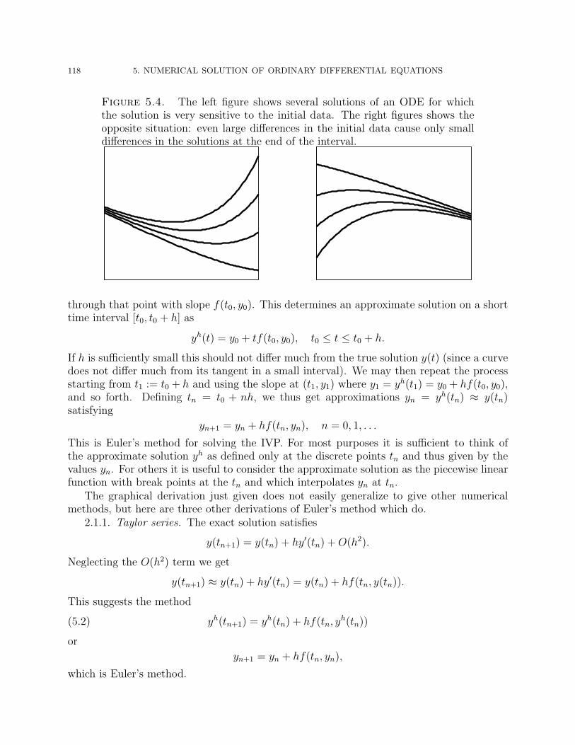
118 5. NUMERICAL SOLUTION OF ORDINARY DIFFERENTIAL EQUATIONS
Figure 5.4. The left figure shows several solutions of an ODE for whichthe solution is very sensitive to the initial data. The right figures shows theopposite situation: even large differences in the initial data cause only smalldifferences in the solutions at the end of the interval.
through that point with slope f(t0, y0). This determines an approximate solution on a shorttime interval [t0, t0 + h] as
yh(t) = y0 + tf(t0, y0), t0 ≤ t ≤ t0 + h.
If h is sufficiently small this should not differ much from the true solution y(t) (since a curvedoes not differ much from its tangent in a small interval). We may then repeat the processstarting from t1 := t0 + h and using the slope at (t1, y1) where y1 = yh(t1) = y0 + hf(t0, y0),and so forth. Defining tn = t0 + nh, we thus get approximations yn = yh(tn) ≈ y(tn)satisfying
yn+1 = yn + hf(tn, yn), n = 0, 1, . . .
This is Euler’s method for solving the IVP. For most purposes it is sufficient to think ofthe approximate solution yh as defined only at the discrete points tn and thus given by thevalues yn. For others it is useful to consider the approximate solution as the piecewise linearfunction with break points at the tn and which interpolates yn at tn.
The graphical derivation just given does not easily generalize to give other numericalmethods, but here are three other derivations of Euler’s method which do.
2.1.1. Taylor series. The exact solution satisfies
y(tn+1) = y(tn) + hy′(tn) +O(h2).
Neglecting the O(h2) term we get
y(tn+1) ≈ y(tn) + hy′(tn) = y(tn) + hf(tn, y(tn)).
This suggests the method
(5.2) yh(tn+1) = yh(tn) + hf(tn, yh(tn))
or
yn+1 = yn + hf(tn, yn),
which is Euler’s method.

2. EULER’S METHOD 119
2.1.2. Numerical differentiation. Approximating the derivative y′(tn) by the forward dif-ference [y(tn+1)− y(tn)]/h gives
y(tn+1)− y(tn)
h≈ f
(tn, y(tn)
),
ory(tn+1) ≈ y(tn) + hy′(tn) = y(tn) + hf
(tn, y(tn)
).
which again suggests Euler’s method.2.1.3. Numerical integration. The exact solution satisfies the integral condition
y(tn+1) = y(tn) +
∫ tn+1
tn
f(t, y(t)
)dt.
Approximating the integral by the left endpoint rule we get, once again,
y(tn+1) ≈ y(tn) + hf(tn, y(tn)
).
2.2. Convergence. In this section we analyze the convergence of Euler’s method. Forsimplicity we assume that f ∈ C(I × R), I = [t0, t
∗], and satisfies a uniform Lipschitzcondition with respect to its second variable (so there is a unique solution defined on all ofI. For any h > 0 define N = Nh = b(t∗ − t0)/hc (so that tN is the largest break point in I),and define yn = yh(tn) for 0 ≤ n ≤ N by Euler’s method. The error is eh = yh− y. We shallmeasure the error in the discrete max norm
‖eh‖∞,h = max0≤n≤Nh
|eh(tn)|,
and determine the behavior of this quantity as h ↓ 0. It would be a small matter, but notnow worth the effort, to use the max norm on the whole interval I.
Theorem 5.4 (Convergence of Euler’s method). limh↓0‖yh − y‖∞,h = 0.
Proof. Define the local truncation error on the (n+ 1)st step by the equation
(5.3) y(tn+1) = y(tn) + hf(tn, y(tn)
)+ Tn.
Thus Tn is the amount by which the exact solution fails to satisfy Euler’s method. It is localto the n+ 1st step in that we compare the exact solution at the end of the step to what wewould have obtained using Euler’s method over the step starting with the exact solution atthe beginning of the step, and ignoring all the accumulated errors up to that point.
By the mean value theorem,
y(tn+1) = y(tn) + hy′(ξn) for some ξn ∈ (tn, tn+1),
while the differential equation gives f(tn, y(tn)
)= y′(tn). Thus
(5.4) Tn = h[y′(ξn)− y′(tn)].
Subtracting (5.3) from (5.2) gives
en+1 = en + h[f(tn, y
h(tn))− f
(tn, y(tn)
)]− Tn.
Setting T = max0≤n≤N−1 |Tn| and using the Lipschitz condition we get
|en+1| ≤ (1 + hL)|en|+ T, 0 ≤ n ≤ N − 1,

120 5. NUMERICAL SOLUTION OF ORDINARY DIFFERENTIAL EQUATIONS
and, since we start with the exact initial value, e0 = 0. We now apply a simple lemma (whichis easily established by induction):
Lemma 5.5. Let A, B, η0, η1, . . . , ηN be non-negative numbers satisfying
ηn+1 ≤ Aηn +B, n = 0, 1, . . . , N − 1.
Then
ηn ≤ Anη0 +(n−1∑
i=0
Ai)B, n = 0, 1, . . . , N.
For A 6= 1 the quantity in parenthesis is equal to (An − 1)/(A− 1).
Applying the lemma, we get
|en| ≤(1 + hL)n − 1
hLT, n = 0, 1, . . . , N.
Since 1 + x ≤ ex for all x, this gives
(5.5) |en| ≤eL|t∗−t0| − 1
L
T
h,
and we have reduced the theorem to showing that limh→0 T/h = 0.Since f is continuous, the solution y′ is uniformly continuous on the closed interval I.
Therefore, give ε > 0 there exists h0 > 0 such that |y′(t) − y′(u)| ≤ ε if t, u ∈ I satisfy|t− u| ≤ h0. In view of (5.4) we have T/h ≤ ε whenever h ≤ h0.
If we require a little extra regularity, we can get an estimate with a rate of convergence.
Theorem 5.6 (Rate of convergence for Euler’s method). If y ∈ C2(I) then
‖yh − y‖∞,h ≤ Ch,
where
(5.6) C = ‖y′′‖∞eL|t∗−t0| − 1
2L.
Proof. By Taylor’s theorem
y(tn+1) = y(tn) + hy′(tn) +h2
2y′′(ξn),
for some ξn. In view of the definition (5.3), Tn = (h2/2)y′′(ξn), and so |T/h| ≤ (h/2)‖y′′‖∞.The theorem therefore follows from (5.5).
The constant C asserted in the preceeding theorem, is often very pessimistic compared tothe outcome of actual computation, but the first order convergence is not. The next theoremshows (assuming a bit more smoothness), that the error at any time does indeed behave likech, up to higher order, for some c.
Theorem 5.7 (Asymptotic error estimate for Euler’s method). Suppose that y ∈ C3(I)and that ∂f/∂y and ∂2f/∂y2 are both continuous. Then there exists a function δ : I → Rindependent of h such that
yh(tn)− y(tn) = δ(tn)h+O(h2), n = 0, 1, . . . , N(h).

2. EULER’S METHOD 121
The function δ is the solution of the linear initial value problem
(5.7) δ′(t) =∂f
∂y
(t, y(t)
)δ(t)− 1
2y′′(t), δ(t0) = 0.
Proof. Using Taylor’s theorem and the definition of Euler’s method we get
en+1 = en + h[f(tn, y
h(tn))− f
(tn, y(tn)
)]− h2
2y′′(tn)− h3
6y′′′(ξn),
for some ξn. Applying Taylor’s theorem to f as a function of y we get
f(tn, y
h(tn))
= f(tn, y(tn)
)+∂f
∂y
(tn, y(tn)
)en +
1
2
∂2f
∂y2(tn, ζn)e2n
for some ζn between y(tn) and yh(tn). Combining these two expansions we get
(5.8) en+1 =
[1 + h
∂f
∂y
(tn, y(tn)
)]en −
h2
2y′′(tn) +Rn
where
Rn = −h3
6y′′′(ξn)− 1
2
∂2f
∂y2(tn, ζn)e2nh.
By the first order convergence of Euler’s method we know that ζn stays bounded for all nand h and that en = O(h). Thus Rn = O(h3).
Now we define gn by replacing en by gn in (5.8) and dropping the term Rn:
(5.9) gn+1 =
[1 + h
∂f
∂y
(tn, y(tn)
)]gn −
h2
2y′′(tn), g0 = 0.
To complete the proof we will show that
gn = δ(tn)h+O(h2),(5.10)
en = gn +O(h2).(5.11)
Now (5.10) is equivalent to
dn = δ(tn) +O(h),
where dn = gn/h. In terms of dn, (5.9) becomes
dn+1 = dn + h
[∂f
∂y
(tn, y(tn)
)dn −
1
2y′′(tn)
], g0 = 0.
which is precisely Euler’s method for the initial value problem (5.7). Thus (5.10) followsfrom Theorem 5.6.
To prove (5.11), let kn = en − gn. Subtract (5.9) from (5.8) to get
kn+1 = [1 + h∂f
∂y
(tn, y(tn)
)]kn +Rn.
Therefore
|kn+1| ≤ (1 +Kh)|kn|+ maxn|Rn| with K = max
t0≤t≤t∗
∣∣∣∣∂f∂y (tn, y(tn))∣∣∣∣ .

122 5. NUMERICAL SOLUTION OF ORDINARY DIFFERENTIAL EQUATIONS
Noting that k0 = 0 and applying Lemma 5.5 we get
|kn| ≤(1 +Kh)n − 1
Khmax |Rn|.
Bounding (1+Kh)n by exp(K|t∗−t0|) and recalling that Rn = O(h3) we obtain the theorem.
Remark. The initial value problem (5.7) is linear so its solution can be written in closedterms:
δ(t) = −1
2ρ(t)
∫ t
t0
y′′(s)
ρ(s)ds, ρ(s) = exp[
∫ t
t0
∂f
∂y
(s, y(s)
)ds].
This is not very useful in practice, since we don’t know y, much less y′′. So the significanceof the theorem is mainly the assertion that the error behaves like δh, not the particular formof δ. This is useful for many purpose, e.g., for Richardson extrapolation.
2.3. Variable step size. There is no reason why the same value of h has to be usedin each step of Euler’s method. We can instead vary h, determining it in advance or as wego along in some adaptive way (adaptive step size selection will be treated in § 5 of thischapter). Euler’s method with variable step size is thus
yh(t0) = y0
for n = 0, 1, . . .choose hn > 0tn+1 = tn + hn
if tn+1 ≤ t∗ thenyh(tn+1) = yh(tn) + hnf
(tn, y
h(tn))
elsestop
end ifend
Let e = yh − y denote the error. We again use the discrete maximum norm:
‖e‖ = max |e(tn)|,where the maximum is taken over the particular mesh points used. We also set H = maxhn,the largest step size. We then again have convergence (we continue to assume that f satisfiesa uniform Lipschitz condition with respect to y), and, if the solution is C2, the convergenceis first order in H:
Theorem 5.8 (Convergence of Euler’s method with variable step). For Euler’s methodwith variable step size
limH→0‖e‖ = 0,
i.e., for all ε > 0 there exists H0 > 0 such that for any choice of steps hn with maxhn ≤ H0
there holds max |e(tn)| ≤ ε.Moreover, if the solution y ∈ C2(I), then ‖e‖ ≤ CH, where C is again defined by (5.6).

3. LINEAR MULTISTEP METHODS 123
The proof of this theorem follows very much along the lines of the proofs of Theorems 5.4and 5.6. The bounds on the local truncation error are the same. Lemma 5.5 which is usedto bound the accumulated contributions of the local truncation errors on all the steps, mustbe generalized as follows.
Lemma 5.9. Let An > 1 and Bn ≥ 0 for n = 0, 1, . . . , N − 1 and let η0, η1, . . . , ηN ≥ 0.Suppose that
ηn+1 ≤ Anηn +Bn, n = 0, 1, . . . , N − 1.
Then
ηn ≤(n−1∏
i=0
Ai
)η0 +
(n−1∏i=0
Ai − 1)
sup0≤i≤n−1
Bi
Ai − 1, n = 1, 2, . . . , N.
The proof of the lemma—which is a straightforward induction—and that of Theorem 5.8,is left to the reader.
Remark. Without some assumption on the way the step sizes are chosen we cannotprove (or even sensibly state) an asymptotic error estimate. One possibility is to assumethat the step sizes are determined using a step size parameter h > 0 and a continuous stepmodification function Θ : I → R+ by the formula hn = Θ(tn)h. That is, as the mesh isrefined the ratio of step sizes in one part of the interval to those in another is determined byΘ. In practice, Θ would reflect the nature of the solution (larger where the solution is verysmooth and smaller where the solution varies rapidly). In this case it is possible to prove anasymptotic error estimate very similar to Theorem 5.7.
3. Linear multistep methods
Euler’s method is an example of a one-step method: the numerical solution yn+1 at tn+1
is determined from the numerical solution at the single preceding point yn. More generally,we can consider methods take a constant step size h and determine yn+1 using the valuesfrom several preceding steps:
yn+1 = Φ(f, tn, yn+1, yn, yn−1, . . . , yn−k, h).
Here yn+1 depends on k+1 previous values, so this is called a k+1-step method. Notice thatwe have allowed yn+1 to appear in the right-hand side of the equation as well as the left. Whenthis happens, we speak of an implicit method, and we need to solve a nonlinear equation todetermine yn+1. In any case, we need to determine the first k+1 values y0, y1, . . . yk by someother method, such as a single step method.
If Φ does not depend on yn+1 we speak of an explicit method. Thus Euler’s method isan explicit one-step method. The backward Euler method
yn+1 = yn + hf(tn+1, yn+1),
and the trapezoidal method
yn+1 = yn +h
2[f(tn+1, yn+1) + f(tn, yn)],
are examples of implicit one-step methods.

124 5. NUMERICAL SOLUTION OF ORDINARY DIFFERENTIAL EQUATIONS
Notice that in each of these cases, the Φ is a linear function of yn, yn+1, f(tn, yn), andf(tn+1, yn+1). By contrast, for the improved Euler method,
yn+1 = yn +h
2[f(tn, yn) + f
(tn+1, yn + hf(tn, yn)
)],
which is an explicit one-step method, and the implicit midpoint method,
yn+1 = yn + hf(tn + tn+1
2,yn + yn+1
2),
which is an implicit one-step method, the dependence of Φ on yn and yn+1 is more compli-cated. In the next section, we shall consider such nonlinear one-step methods, while in thissection we study multistep methods, but assume linear dependence. That is, we considerlinear multistep methods with constant step size, which, by definition, are methods of theform
(5.12) yn+1 = −a0yn − a1yn−1 + · · · − akyn−k + h[b−1fn+1 + b0fn + · · ·+ bkfn−k].
Here we have written fn for f(tn, yn) (for brevity). The ai and bi are constants which mustbe given and determine the specific method. For an explicit linear multistep method b−1 = 0.It is also convenient to define a−1 = 1, so that the method can be written
k∑j=−1
ajyn−j = hk∑
j=−1
bjfn−j.
One obvious question concerning implicit methods is whether the formula for the methoddetermines yn+1 (whether the equation has a solution and whether it is unique). The answeris yes, at least for h sufficiently small.
Theorem 5.10. Let h0 = (|b−1|L)−1 where L is the Lipschitz constant for f . Then forany h < h0 and any yn, yn−1, . . . , yn−k there is a unique yn+1 such that
(5.13)k∑
j=−1
ajyn−j = hk∑
j=−1
bjf(tn−j, yn−j).
Proof. Define
F (z) = −k∑
j=0
ajyn−j + hb−1f(tn+1, z) + h
k∑j=0
bjf(tn−j, yn−j) = hb−1f(tn+1, z) + · · · ,
where the dots represent terms not depending on z. Then the equation is simply the fixedpoint equation yn+1 = F (yn+1). Now F is a Lipschitz with Lipschitz constant ≤ h|b−1|L.By hypothesis the Lipschitz constant is stritly less than 1, i.e., F is a contraction. Thecontraction mapping theorem then guarantees a unique fixed point.
Remark. The contraction mapping theorem also implies that the solution can be com-puted by fixed point iteration, and this is often done in practice. Of course only finitelymany iterations are made (often quite few), introducing an additional source of error.
Several examples of linear multistep methods are listed in Table 5.1. All the methodsin the table except the last can be derived from the integral relation y(tn+1) = y(tn−k) +∫ tn+1
tn−if(t, y(t)
)dt using an appropriate interpolatory quadrature rule. Note that for the two

3. LINEAR MULTISTEP METHODS 125
Table 5.1. Examples of linear multistep methods.
Euler’s method (1-step, explicit) yn+1 = yn + hfn
backward Euler method (1-step, implicit) yn+1 = yn + hfn+1
trapezoidal method (1-step, implicit) yn+1 = yn +h
2(fn+1 + fn)
midpoint method (2-step, explicit) yn+1 = yn−1 + 2hfn
Milne–Simpson method (2-step, implicit) yn+1 = yn−1 +h
3(fn+1 + 4fn + fn−1)
Adams–Bashford 2-step method (explicit) yn+1 = yn +h
2(3fn − fn−1)
Adams–Moulton 2-step method (implicit) yn+1 = yn +h
12(5fn+1 + 8fn − fn−1)
3-step backward differentiation formula (implicit) yn+1 − 19yn + 9yn−1 − 2yn−2 = 6fn+1
Adams methods (the Adams–Bashford and Adams–Moulton families of methods will be dis-cussed in detail in § 3.3 below) the quadrature rule is open, i.e., contains quadrature pointsoutside the interval of integration. The final method of the table is one of the backward differ-entiation formula, or BDF, family of methods, which can be derived by replacing y′(tn+1) inthe equation y′(tn+1) = f
(tn+1, y(tn+1)
)with a backward difference approximation obtained
by differentiating an interpolating polynomial.
3.1. Consistency and order. Clearly the coefficients aj and bj in (5.12) must be chosencarefully if the multistep method is to have a chance of being convergent. Specifically, weshould have
k∑j=−1
ajy(tn−j) ≈ hk∑
j=−1
bjy′(tn−j)
for the exact solution y. Since this has to hold for any solution to any ODE, it should holdfor all reasonably smooth functions y. Thus we define
(5.14) L[y, h, t] =k∑
j=−1
ajy(t− jh)− hk∑
j=−1
bjy′(t− jh)
for any y ∈ C1, h > 0 and t ∈ R. Note that if y is the exact solution, then L[y, h, tn] issimply the local truncation error at the (n+ 1)st step.
Definition. The linear multistep is consistent if
limh↓0
maxk≤n<N
∣∣∣∣L[y, h, tn]
h
∣∣∣∣ = 0

126 5. NUMERICAL SOLUTION OF ORDINARY DIFFERENTIAL EQUATIONS
for all y ∈ C1(I). The method has order p (at least) if for all y ∈ Cp+1(I) there existsconstants C, h0 > 0 such that
maxk≤n<N
∣∣∣∣L[y, h, tn]
h
∣∣∣∣ ≤ Chp
whenever h < h0.
Warning: it is not true that every method of order p converges with order p, or evenconverges at all!
Using Taylor’s theorem, we can derive simple algebraic criteria for consistency and order.
Theorem 5.11. A linear multistep method is consistent if and only if
(5.15)k∑
j=−1
aj = 0,k∑
j=−1
jaj +k∑
j=−1
bj = 0.
The method is of order p if and only if
(5.16)k∑
j=−1
(−j)maj −mk∑
j=−1
(−j)m−1bj = 0, m = 0, 1, . . . , p.
The algebraic conditions (5.15) are called the consistency conditions and the conditions(5.16) are called the order conditions. Before giving the proof we notice an immediatecorollary: a method is consistent if and only if it is of order at least 1.
Proof. The proof is just Taylor’s theorem. We have y(tn − jh) = y(tn) − jhy′(ξj), forsome ξj ∈ [tn − kh, tn + h], j = −1, 0, . . . , k. Note that each ξj → t as h→ 0. Plugging into(5.14)
L[y, h, tn] =k∑
j=−1
aj[y(tn)− jhy′(ξj)]− hk∑
j=−1
bjy′(tn − jh)
= y(tn)C0 + hy′(tn)C1 + hR,
where
C0 =k∑
j=−1
aj, C1 = −k∑
j=−1
jaj −k∑
j=−1
bj,
and
R = −hk∑
j=0
jaj[y′(ξj)− y′(tn)]− h
k∑j=−1
bj[y′(tn − jh)− y′(tn)].
By the uniform continuity of y′, we see that R/h→ 0 as h→ 0. Therefore L[y, h, tn]/h→ 0if and only if C0 = C1 = 0, i.e., the consistency conditions are satisfied.

3. LINEAR MULTISTEP METHODS 127
Similarly, if y ∈ Cp+1 we have
y(tn − jh) =
p∑m=0
(−j)m
m!hmy(m)(tn) +
(−j)p+1
(p+ 1)!hp+1y(p+1)(ξj),
y′(tn − jh) =
p∑m=1
(−j)m−1
(m− 1)!hm−1y(m)(tn) +
(−j)p
p!hpy(p+1)(ζj),
for some ξj, ζj ∈ [tn − kh, tn + h]. This gives
L[y, h, tn] =
p∑m=0
hmy(m)(tn)Cm +R,
where
(5.17) Cm =1
m!
[ k∑j=−1
(−j)maj −mk∑
j=−1
(−j)m−1bj
],
and
R = hp+1
k∑j=−1
[aj(−j)p+1
(p+ 1)!y(p+1)(ξj)− bj
(−j)p
p!y(p+1)(ζj)].
Since R = O(hp+1), L/h = O(hp) if and only if all the Cm vanish.
Remark. This theorem furnishes an example of how a complicated analytic conditionmay sometimes be reduced to a simple algebraic criterion. Many such criteria for multistepmethods can be expressed in terms of the characteristic polynomials of the method:
ρ(z) =k∑
j=−1
ajzk−j, σ(z) =
k∑j=−1
bjzk−j.
For example, the consistency conditions are simply ρ(1) = 0 and ρ′(1) = σ(1).
As an example of the use of the order conditions, we will use the method of undeterminedcoefficients to find the 2-step method of highest order. For a 2-step method there are fiveundetermined coefficients: a0, a1, b−1, b0, and b1. The first five order conditions are
1 + a0 + a1 = 0, 1− a1 − b−1 − b0 − b1 = 0, 1 + a1 − 2b−1 + 2b1 = 0,
1− a1 − 3b−1 − 3b1 = 0, 1 + a1 − 4b−1 + 4b1 = 0.
This system of linear equations has a unique solution:
a0 = 0, a1 = −1, b−1 =1
3, b0 =
4
3, b1 =
1
3,
which are precisely the coefficients of the Milne-Simpson method. Thus the Milne-Simpsonmethod is the unique fourth order 2-step method.
If we consider instead explicit 2-step methods we no longer have the coefficient b−1 atour disposal. Setting b−1 to zero in the first four linear equations above we get
1 + a0 + a1 = 0, 1− a1 − b0 − b1 = 0, 1 + a1 + 2b1 = 0, 1− a1 − 3b1 = 0,

128 5. NUMERICAL SOLUTION OF ORDINARY DIFFERENTIAL EQUATIONS
which gives a0 = 4, a1 = −5, b0 = 4, b1 = 2. Thus the unique explict 2-step method of order3 is
yn+1 + 4yn − 5yn−1 = h[4fn + 2fn−1].
Warning: we shall see below that this is not a good method. Order is not everything!
3.2. Stability and convergence. In this section we study the convergence of linearmultistep methods. Recalling that the initial k+1 values of yh
n must be determined by someother method, we define convergence as follows.
Definition. A linear multistep method is convergent if whenever the initial values yhn
are chosen so that max0≤j≤k |ehj | → 0 as h→ 0, then max0≤j≤Nh |eh
j | → 0.
There is a rather complete convergence theory available for linear multistep methods withconstant step size, due largely to G. Dahlquist. It is somewhat technical, and we will onlysketch it below. However, for many linear multistep methods a simple proof of convergencecan be given along the lines of the proof we used for Euler’s method. For example, considerthe midpoint method
yn+1 = yn−1 + 2hf(tn, yn).
Checking the order conditions we find that this method is second order, i.e., if y is a smoothfunction, then
y(tn+1) = y(tn−1) + 2hy′(tn) + L[y, h, tn]
where L[y, h, tn] = O(h3). Now let en = yn − y(tn). Then
en+1 = en−1 + 2h[f(tn, yn)− f(tn, y(tn)
)]− L[y, h, tn],
so
|en+1| ≤ |en−1|+ 2hL|en|+ T, n = 1, 2, . . . , N − 1,
where T = max |L[y, h, tn]| = O(h3). This immediately implies that
max(|en+1|, |en|) ≤ (1 + 2hL) max(|en|, |en−1|) + T, n = 0, 1, 2, . . . , N − 1,
whence, by Lemma 5.5,
max(|en+1|, |en|) ≤e2L|t∗−t0| − 1
2L
T
h+ e2L|t∗−t0| max(|e1|, |e0|), n = 0, 1, 2, . . . , N − 1,
i.e., ‖e‖∞,h ≤ C1T/h + C2 max(|e1|, |e0|) with C1, C2 independent of h. If the initial valuesare choosen so that max(|e1|, |e0|) → 0 as h → 0, then we have that ‖e‖∞,h → 0. Thisis precisely the definition of convergence. For the midpoint method we see as well, that ifthe initial error is O(h2) the error is globally O(h2). Note the one new idea of the proof:instead of considering the propagation of the error (en−1, en) 7→ en+1, we instead considerthe propagation of the pair of values, (en−1, en) 7→ (en, en+1).
Next we consider the two step method of highest order
yn+1 = −4yn + 5yn−1 + h(4fn + 2fn−1).
We shall show that this method is not convergent even for the most trivial of initial valueproblems:
y′(t) = 0, 0 ≤ t ≤ 1, y(0) = 0.

3. LINEAR MULTISTEP METHODS 129
The multistep method is then yn+1 = −4yn + 5yn−1. If we take as initial values y0 = 0,y1 = εh, then the multistep method is easily seen to give
yn = [1− (−5)n]εh/6,
and so, if h = 1/N , yh(1) = yN = [1 − (−5)1/h]εh/6. It is clearly not sufficient that εh → 0in order to have convergence, we need 51/hεh → 0, i.e., exponentially accurate initial values.
Note that if we take exact starting values y0 = y1 = 0, then yn = 0 for all n. Thus aperturbation of size ε in the starting values leads to a difference of size roughly 51/hε in thediscrete solution. Thus the method is not stable:
Definition. A linear k + 1-step method is stable if for any admissable initial valueproblem (satisfying a Lipschitz condition) and for all ε > 0 there exists δ, h0 > 0 such thatif h ≤ h0 and two choices of starting values yj and yj are chosen satisfying
max0≤j≤k
|yj − yj| ≤ δ,
then the corresponding approximate solutions satisfy
max0≤j≤N
|yj − yj| ≤ ε.
If, as above, we consider the trivial differential equation y′ = 0, then the general linearmultistep method becomes
yn+1 +k∑
j=0
ajyn−j = 0, n = k, k + 1, . . . .
This is an example of a homogeneous linear difference equation of order k + 1 with constantcoefficients. For such an equation there is a simple approach to finding the general solutionin closed form, which we shall now briefly present. We shall allow complex solutions. Thenthere is clearly a unique solution (yn)∞n=0 for any choice of initial values (yn)k
n=0 ∈ Ck+1.Thus the space of solutions is a complex vectorspace of dimension k + 1.
To find the general solution, we first try for a solution of the form (λn)∞n=0. Pluggingthis into difference equation, we see that it is a solution if and only if λ is a root of thecharacteristic polynomial ρ(t) = tk+1 +
∑kj=0 ajt
k−j. If there are k + 1 distinct roots λi,i = 0, . . . , k, we obtain a full basis of k+1 linearly independent solutions in this way. To seelinear independence, notice that the matrix of initial values (λn
i )0≤i,n≤k is a Vandermondematrix, and so nonsingular. In the case of multiple roots this does not give a complete setof solutions. In the case where λ is a double root, we obtain, in addition to the solution(λn)∞n=0 the solution (nλn)∞n=0. For a triple root we find that (n2λn)∞n=0 is a solution aswell, and so forth. In this case we obtain a complete set of solutions in terms of the rootsof the characteristic polynomial. We illustrate with a simple example unrelated to linearmultistep methods. The difference equation yn+1 = yn + yn−1 together with the initialconditions y0 = 0, y1 = 1 defines the Fibonacci sequence. The characteristic polynomial ofthe difference equation is ρ(t) = t2 − t− 1 with roots (1±
√5)/2. Thus the general solution
is yn = c0[(1 −√
5)/2]n + c1[(1 +√
5)/2]n. Imposing the initial conditions y0 = y1 = 1 we

130 5. NUMERICAL SOLUTION OF ORDINARY DIFFERENTIAL EQUATIONS
find Binet’s formula for the nth Fibonacci number:
yn =1√5
[(1 +√
5
2
)n
−
(1−√
5
2
)n].
Returning to linear multistep methods, consider again the trivial differential equationy′ = 0, so the method reduces to a homogeneous linear difference equation. If the firstcharacteristic polynomial has a root of modulus greater than 1, then the difference equationwill have exponentially growing solutions, and so yh(1) which equals yN when h = 1/N , willgrow exponentially unless the initial values are chosen to exactly suppress the coefficient ofthis solution. Thus the method will not be stable. The same is true if the characteristicpolynomial has a multiple root of modulus 1, although the instability will be much less severebecause the growth will be algebraic rather than exponential. These considerations lead tothe following definition and theorem, another example in which a complex analytic conditionfor the behavior of a linear multistep condition is reduced to a simple algebraic condition.
Definition. A linear multistep method satisfies the root condition if
(1) every root of its first characteristic polynomial has modulus ≤ 1,(2) all roots of modulus 1 are simple.
Theorem 5.12. A stable linear multistep method satisfies the root condition. If a con-sistent linear multistep method satisfies the root conditions, it is stable.
The considerations above lead to the proof that the root condition is necessary for sta-bility. To prove the reverse implication (which obviously lies deeper, since it concerns anarbitrary differential equation, and not just the trivial equation y′ = 0), will be discussedbelow.
We now state the fundamental convergence theorem for linear multistep methods. Inview of Theorems 5.11 and 5.12, this theorem states that it can be determined whether ornot a linear multistep method is convergent simply by checking some algebraic conditionsconcerning its characteristic polynomials.
Theorem 5.13. A linear multistep method is convergent if and only if it is consistentand stable.
We only sketch the proof. The statement consists of three parts:
• convergence implies consistency,• convergence implies stability,• consistency and stability imply convergence.
The first statement is easy. For the trivial initial value problem y′ = 0, y(0) = 1,The first two statements are straightforward (assuming Theorem 5.12). They can be
proven considering only the simple differential equations y′ = 0, for the root condition andthe first consistency condition, and y′ = 1, for the second consistency condition. The difficultpart is the third part (and the second statement in Theorem 5.12 is proven in the same way).To show the main idea, we prove it in the case of an explicit two step method (most of theideas of the full proof arise already in this case).
We write the two step method
yn+1 = −a0yn − a1yn−1 + h(b0fn + b1fn−1)

3. LINEAR MULTISTEP METHODS 131
in matrix form: (yn
yn+1
)=
(0 1−a1 −a0
)(yn−1
yn
)+
(0
h(b0fn + b1fn−1)
).
The exact solution satisfies a similar equation with the addition of the local truncation error:(y(tn)y(tn+1)
)=
(0 1−a1 −a0
)(yn−1
yn
)+
(0
h[b0f(tn, y(tn)
)+ b1f
(tn−1, y(tn−1)
)] + L[y, h, tn]
).
Subtracting gives an equation for the error. Let
en = yn − y(tn), En =
(en−1
en
), A =
(0 1−a1 −a0
),
Qn =
(0
h[b0fn − f(tn, y(tn)
)+ b1fn−1 − f
(tn−1, y(tn−1)
)]− L[y, h, tn]
).
Then
(5.18) En+1 = AEn +Qn, n = 1, 2, . . .
Note that ‖Qn‖ ≤ Ch‖En‖+ T where T = maxn |L[y, h, tn]| = O(hp+1) where p is the orderof the method (and we use the l∞ norm for the vectors). Iterating (5.18) gives
En = An−1E1 +n−1∑j=1
An−1−jQj, n = 1, . . . , N.
Now we use the root condition. The characteristic polynomial of the matrix A is ρ(t) =t2 + a0t + a1, i.e., the first characteristic polynomial of the linear multistep method. Thusthe eigenvalues of A all have modulus ≤ 1 with only simple eigenvalues of modulus 1. Thisis precisely the condition for the powers of A to remain bounded: supn≥0‖An‖ < ∞. Thuswe have
‖En‖ ≤ C(‖E1‖+n−1∑j=1
‖Qj‖) ≤ C ′(hn−1∑j=1
‖Ej‖+ ‖E1‖+T
h), n = 1, . . . , N,
for some constants C and C ′. Now from this relation it follows (by a sort of discrete Gronwalllemma1 that
max1≤n≤N
‖En‖ ≤ K(‖E1‖+T
h),
for a suitable constant K. For a consistent method T/h → 0 as h → 0, so convergencefollows.
We end this section with a statement of the attainable order of multistep methods.Counting coefficients and order conditions one would guess (correctly) that the highest orderattainable by a k step method is 2k. However, such a method is not stable for any k > 1.The next theorem states that only about half this order is attainable by a stable method.
1Specifically, if ξm ≤ αm−1∑j=1
ξj + β, m = 1, 2, . . ., where the ξm, α, and β are non-negative, then ξm ≤
β(1 + α)m−1.

132 5. NUMERICAL SOLUTION OF ORDINARY DIFFERENTIAL EQUATIONS
Theorem 5.14 (First Dahlquist barrier). The highest order of a stable k step method isk + 1 if k is odd and k + 2 if k is even.
3.3. Adams methods. The Adams methods are linear multistep methods with thebest possible stability properties. Namely the first characteristic polynomial has all its rootsat the origin except for the mandatory root at 1. That is, the first characteristic polynomialof a k+1 step Adams method is ρ(t) = tk+1− tk. There are two Adams methods for each k,an explicit method, called an Adams–Bashford method, and an implicit method, called anAdams–Moulton method. They can be derived by quadrature as follows. We start with theequation
y(tn+1) = y(tn) +
∫ tn+1
tn
f(t, y(t)
)dt.
Now, assuming that yj is known for j ≤ n, let P (t) ∈ Pk denote the Lagrange interpolatingpolynomial satisfying P (tj) = fj := f(tj, yj), j = n, n− 1, . . . , n− k. We then define
yn+1 = yn +
∫ tn+1
tn
P (t) dt,
which is the k + 1 step Adams–Bashford method. For k = 0, 1, and 2, the formulas are
yn+1 = yn + hfn, (Euler’s method)
yn+1 = yn + h(3
2fn −
1
2fn−1),
yn+1 = yn + h(23
12fn −
4
3fn−1 +
5
12fn−2).
Using Lagrange’s formula for the interpolating polynomial, we can easily find the generalformula
yn+1 = yn + hk∑
j=0
bjfn−j,
where
bj =1
h
∫ tn+1
tn
∏0≤m≤k
m6=j
t− tn−m
tn−j − tn−m
dt =
∫ 1
0
∏0≤m≤k
m6=j
m+ t
m− jdt.
(Note that the first expression can be used also in the case of non-constant step size.)The Adams–Moulton methods are constructed similarly, except that P ∈ Pk+1 interpo-
lates fn−j at tn−j for j = −1, . . . , k. The first few formulas are
yn+1 = yn + h(1
2fn+1 +
1
2fn), (trapezoidal method)
yn+1 = yn + h(5
12fn+1 +
2
3fn −
1
12fn−1),
yn+1 = yn + h(3
8fn+1 +
19
24fn −
5
24fn−1 +
1
24fn−2).
We may also think of the backward Euler method as an Adams–Moulton method withk = −1.

3. LINEAR MULTISTEP METHODS 133
It is easy to check the order of the Adams methods. E.g., for the k + 1 step Adams–Bashford method
L[y, h, tn] =
∫ tn+1
tn
[y′(t)− P (t)] dt,
where P ∈ Pk interpolates y′ at tn, . . . , tn−k. By the Newton error formula for Lagrangeinterpolation,
y′(t)− P (t) = y′[tn, . . . , tn−k, t](t− tn) · · · (t− tn−k),
so, using the integral mean value theorem,
L[y, h, tn] = y′[tn, . . . , tn−k, ξ]
∫ tn+1
tn
(t− tn) · · · (t− tn−k) dt
=1
(k + 1)!y(k+2)(η)
∫ tn+1
tn
(t− tn) · · · (t− tn−k) dt.
for some ξ. The integral is clearly order O(hk+2), so the method is of order k + 1. In factit equals γk+1h
k+2 where γ1 = 1/2, γ2 = 5/12, γ3 = 3/8, . . . . Thus for the Adams–Bashfordmethods, the order is equal to the number of steps.
Similarly, for k step Adams–Moulton method also has order k+1 and the local truncationerror satisfies
L[y, h, tn] =1
(k + 1)!y(k+1)(η)γ∗k+1h
k+2.
The first few γ∗k are γ∗0 = −1/2 (for backward Euler), γ∗1 = −1/12 (for trapezoidal), γ∗2 =−1/24, . . . . Thus to achieve the same order k + 1 we can use a k + 1 step Adams–Bashfordmethod or a k step Adams–Moulton method. The coefficient of hk+2 in the local truncationerror is significantly smaller for the Adams–Moulton method. When we study the notion ofabsolute stability later, we shall find other advantages of the Adams–Moulton methods overthe Adams–Bashford methods.
3.4. Predictor-corrector schemes. To implement an Adams–Moulton method, orany implicit method, we need a way to solve, at least approximately, the nonlinear equationarising at each time step. The most common method is to solve this equation approximatelyusing a small number of fixed point iterations starting from an initial approximation obtainedby an explicit method. Thus the scheme takes the form:
1. predict: pn+1 = E(yn, yn−1, . . . , fn, fn−1, . . .)
2. evaluate: fpn+1 = f(tn+1, pn+1)
3. correct: y(1)n+1 = I(yn, yn−1, . . . , f
pn+1, fn, fn−1, . . .)
4. evaluate: f(1)n+1 = f(tn+1, y
(1)n+1)
5. correct: y(2)n+1 = I(yn, yn−1, . . . , f
(1)n+1, fn, fn−1, . . .)
6. evaluate: f(2)n+1 = f(tn+1, y
(2)n+1)
...
Here E(yn, yn−1, . . . , fn, fn−1, . . .) refers to some explicit scheme, e.g., an Adams–Bashfordscheme, and I(yn, yn−1, . . . , fn+1, fn, . . .) to some implicit, e.g., Adams–Moulton, scheme. At

134 5. NUMERICAL SOLUTION OF ORDINARY DIFFERENTIAL EQUATIONS
some point we stop and declare yn+1 = y(m)n+1. We could stop in response to some stopping
criterion, but more commonly, a fixed, usually small, number of iterations are made. For
example, we may stop the iteration after step 4, and accept y(1)n+1. This would then be
referred to as a PECE scheme. Other possibilities are PECECE, P(EC)3E, etc. As a simpleexample, consider the PECE method with a 2 step Adams–Bashford predictor and a 2 stepAdams–Moulton corrector. This gives
pn+1 = yn + h[3f(tn, yn)− f(tn−1, yn−1)]/2,
yn+1 = yn + h[5f(tn+1, pn+1) + 8f(tn, yn)− f(tn−1, yn−1)]/12.
Thus
yn+1 = yn+h[5f(tn+1, yn+h[3f(tn, yn)−f(tn−1, yn−1)]/2
)+8f(tn, yn)−f(tn−1, yn−1)
]/12.
Thus the resulting method is a nonlinear 2 step method.The analysis of the error of such a scheme is relatively straightforward. We just briefly
sketch the main ideas for a PECE scheme. There are two contributions to the local trun-cation error, one arising from predictor formula and one arising from the corrector formula.If the predictor formula has order p and the corrector formula has order q, so their localtruncation errors are O(hp+1) and O(hq+1) respectively, then the local truncation error forthe PECE scheme will be O(hp+2) + O(hq+1) = O(hmin(p+2,q+1)). The extra order in predic-tor contribution comes from the fact that the term f(tn+1, pn+1) involving the predictor ismultiplied by h in the formula for yn+1. Thus if p ≥ q− 1, the local truncation error will beO(hq+1) just as if the predictor equation were solved exactly. In fact, if we take p ≥ q, thelocal truncation error for the PECE scheme will be asymptotically equal to that for the fullimplicit scheme (i.e., they will agree up to terms of higher order). Thus the most commonchoices are either p = q − 1 or p = q. For a PECE scheme based on Adams methods, wemight use the k step Adams–Bashford for predictor (order k) and the k step Adams–Moultonfor corrector (order k + 1), and thus achieve a method of order k + 1. Or we might take ak + 1 step Adams–Bashford predictor, which would still achieve the same order, but whichwe would expect to have an asymptotically smaller error. Yet another possibility is to use aPECECE scheme with k step Adams methods for both predictor and corrector. This wouldagain produce asymptotically the same error as the fully implicit k step Adams–Moultonmethod.
4. One step methods
We have seen three linear one step methods thus far:
yn+1 = yn + hfn, (Euler’s method)
yn+1 = yn + hfn+1, (backward Euler method)
yn+1 = yn + h(1
2fn+1 +
1
2fn). (trapezoidal method)
Actually these are all special cases of the θ-method
yn+1 = yn + h[(1− θ)fn+1 + θfn],
which is a consistent stable linear 1 step method for any real θ (of course, all consistent 1step methods are stable). Except for Euler’s method, all these methods are implicit.
4. ONE STEP METHODS 135
We may also obtain an explicit, but nonlinear, single step method using Euler as apredictor and one of the other methods as a corrector in a PECE (or PECECE, . . . ) scheme.E.g., with the trapezoidal method as corrector, we get
yn+1 = yn + h[f(tn, yn) + f(tn+1, yn + hf(tn, yn)
)]/2,
which is known as the improved Euler method or Heun’s method.An example of an implicit, nonlinear single step method is a variant of the theta method:
yn+1 = yn + hf((1− θ)yn+1 + θyn
).
All single step methods may be written in the form
yn+1 = yn + hΦ(f ; tn, yn, h),
where Φ is called the relative increment function. For an explicit method, Φ(f ; tn, yn, h) isan explicit function of tn and yn involving f and h. For implicit methods, Φ(f ; tn, yn, h) isgiven in terms of the solution to an algebraic equation. In fact we can even consider theexact relative increment function
∆(f ; tn, yn, h) =y(tn+1)− y(tn)
h,
where u is the exact solution to the differential equation u′(t) = f(t, y(t)
), y(tn) = yn. This
one step method gives the exact solution, but is not implementable. A single step methodwith increment function Φ is of order p (its local truncation error is O(hp+1)) if and only if
Φ(f ; tn, yn, h) = ∆(f ; tn, yn, h) +O(hp).
4.1. Taylor series methods. In a sense, there is a canonical pth order one step method.Taylor’s theorem tells us that
y(t+ h) = y(t) + hy′(t) + · · ·+ hp
p!y(p)(t) +O(h(p+1)).
Now the differential equation tells us that y′(t) = f(t, y(t)
). But we can also differentiate
the differential equation to get
y′′(t) =∂f
∂t
(t, y(t)
)+ f(t, y(t)
)∂f∂y
(t, y(t)
),
or, briefly, y′′ = ft + ffy =: Df , the total derivative of f . Differentiating again gives
y′′′ = ftt + 2ffty + ftfy + ff 2y + f 2fyy =: D2f,
y(4) = D3f , etc. (The expressions for the total derivatives get very complicated, very quickly.)The p-term Taylor series method is the single step method
yn+1 = yn + hfn +h2
2Dfn + · · ·+ hp
p!Dp−1fn,
which clearly has order p. This method can be implemented in some cases, but it requiresevaluation of the partial derivatives of f , and is not commonly used.

136 5. NUMERICAL SOLUTION OF ORDINARY DIFFERENTIAL EQUATIONS
4.2. Runge–Kutta methods. Now let us return to Heun’s method, which we derivedas a PECE scheme with Euler’s method as predictor and the trapezoidal method as corrector.The relative increment function is
Φ = [f(tn, yn) + f(tn+1, yn + hf(tn, yn)
)]/2.
Expanding the second term in brackets in a Taylor polynomial around (tn, yn) we get
Φ = f +h
2(ft + ffy) +O(h2),
where the f and its derivatives are evaluated at (tn, yn). Comparing with the Taylor expan-sion of the exact relative increment we see that Φ = ∆ + O(h2), and hence Heun’s methodis second order. (If we expand Φ out to terms of order h2, we get
Φ = f +h
2(ft + ffy) +
h2
4(ftt + 2ffty + f 2fyy) +O(h3).
The coefficient of h2 does not agree with D2f/3!, so Heun’s method is definitely not of higherthan second order.
Heun’s method is an explicit single step method which requires 2 evaluations of f perstep (but does not require knowledge of the derivatives of f). This is an example of aRunge–Kutta (RK) method. The general form of an explicit RK method is
yn+1 = yn + h(b1φ1 + · · ·+ bqφq),
where φi = f(tn + cih, ηi) and
η1 = yn,
η2 = yn + ha2,1φ1,
η3 = yn + h(a3,1φ1 + a3,2φ2),
...
ηq = yn + h(aq,1φ1 + aq,2φ2 + · · ·+ aq,q−1φq−1).
To specify a particular method of this form we must give the number of stages q ≥ 1, thecoefficients bi, ci, 1 ≤ i ≤ q, and aij, 1 ≤ i ≤ q, 1 ≤ j < i. The bi are called the weights, theci (or the points tn + cih) the nodes, and the ηi, or, sometimes, the φi, are called the stagesof the RK method. Thus, a RK method is specified by weight and node vectors, b, c ∈ Rq,and a strictly lower triangular matrix A ∈ Rq×q. These are often recorded in a RK tableauthus:
c A
bT
The tableau for Heun’s method is
01 1
12
12

4. ONE STEP METHODS 137
where we don’t bother to write the zeros in the upper triangle of A. Other well-known RKmethods are the modified Euler method, Heun’s 3 stage method, and the Runge–Kutta–Simpson 4-stage method (often referred to as the Runge–Kutta method), whose tableauxare
012
12
0 1
012
12
1 −1 2
16
23
16
012
12
12
0 12
1 0 0 1
16
13
13
16
respectively. For any of these methods, it is an elementary, but tedious computation (easilycarried out by a computer algebra program) to determine their order by an expansion inTaylor series. One finds that the modified Euler method is of order 2, Heun’s 3-stage methodis of order 3, and the Runge–Kutta-Simpson method is of order 4. These are the highestpossible orders achievable with the given number of stages. That is, it can be verified, bysimilarly tedious computation, that the highest order achievable by a Runge–Kutta methodwith q stages is q for each q from 1 to 4. However for q from 5 to 7 order q − 1 is thebest achievable, and for q = 8, order 6 is the best achievable. Butcher has developed graphtheoretic techniques for constructing and analyzing RK methods which are necessary whenworking with more than a modest number of stages.
It is also possible to use implicit Runge–Kutta methods. These are defined by the sameequations, except that the coefficient matrix A is no longer required to be lower triangular.This requires the solution of a coupled system of q nonlinear equations to determine the ηi
at each step (and if, as is usually the case, we are solving a system of, say, d, ODEs, each ηi
is itself a vector with d components, and we have to solve a system of qd coupled nonlinearalgebraic equations). For this reason one rarely uses implicit RK methods with more than afew stages.
4.3. Convergence of single step methods. We now consider the convergence of thegeneral single-step method
yn+1 = yn + hΦ(f ; tn, yn, h).
We assume as usual that f(t, y) belongs to C([t0, t∗] × R) and satisfies a uniform Lipschitz
condition with respect to y. We assume that the relative increment function Φ(f ; t, y, h),which is defined for t ∈ [t0, t
∗], y ∈ R, h ∈ [0, t∗ − t], is continuous there. Moreover weassume the uniform Lipschitz condition
|Φ(f ; t, y, h)− Φ(f ; t, y, h)| ≤ K|y − y|,
whenever (t, y, h) and (t, y, h) belong to the domain of Φ. For Taylor series methods it iseasy to deduce the continuity and Lipschitz condition for Φ for smooth f . For Runge–Kuttamethods continuity is evident and the Lipschitz condition is not hard to obtain using thesame condition for f .
A single step method with relative increment function Φ is consistent if
limh↓0
[Φ(f ; t, y, h)−∆(f ; t, y, h)] = 0.

138 5. NUMERICAL SOLUTION OF ORDINARY DIFFERENTIAL EQUATIONS
In view of continuity we can state this simply as Φ(f ; t, y, 0) = f(t, y). The method hasorder p if |Φ(f ; t, y, h)−∆(f ; t, y, h)| ≤ Chp (whenever f is smooth).
Theorem 5.15. A single step method is convergent if and only if it is consistent.
Proof. Define yh by the single step method:
yh(tn+1) = yh(tn) + hΦ(f ; tn, y
h(tn), h),
starting from yh(t0) = y0. We claim that, whether or not the method is consistent, as h→ 0yh converges to the solution of the boundary value problem
z′(t) = g(t, z(t)
), z(t0) = y0,
where g(t, y) = Φ(f ; t, y, 0). Since, by definition, the method is consistent if and onlyif f = g, this will prove the theorem. (If f(t, y) 6= g(t, y) for some (t, y), then we lety(t) be the solution to y′ = f(t, y) passing through y at t. Then either y(t) 6= z(t) ory′(t) = f(t, y) 6= g(t, y) = z′(t), so, in either case, z 6≡ y.)
To prove the claim, note that
z(tn+1) = z(tn) + hz′(ξn) = z(tn) + hg(ξn, z(ξn)
),
for some ξn ∈ (tn, tn+1). Putting en = z(tn)− yh(tn) and subtracting we get
en+1 = en + h[g(ξn, z(ξn)
)− Φ
(f ; t, yh(tn), h
)].
Now the term in brackets may we decomposed as
[g(ξn, z(ξn)
)− g(tn, z(tn)
)]
+[Φ(f ; tn, z(tn), 0)− Φ(f ; tn, z(tn), h
)]
+[Φ(f ; tn, z(tn), h
)− Φ
(f ; tn, y
h(tn), h)].
The first two terms tend to 0 with h by uniform continuity of g and Φ, and the last termcan be bounded by K|en| using the Lipschitz condition. Thus we have
|en+1| ≤ (1 +Kh)|en|+ ω(h),
where limh→0 ω(h) = 0. Since we also have e0 = 0, it follows, in the usual way, that thesequence en tends to 0.
5. Error estimation and adaptivity
Just as for numerical quadrature, a code for the numerical solution of ordinary differentialequations can be much more efficient if the step size is adjusted adaptively to the solution.Very roughly speaking, in parts of its domain where the solution is rapidly varying, and sohas large derivatives, a smaller step size will be needed than in places where the solutionis more slowly varying. In this section we will study the main ideas behind some modernadaptive ODE solvers.
The first step in designing an adaptive solver is to establish the goal of the solver. In manycases the user may wish to control some global error measure, like the discrete maximumnorm error
max0≤n≤N
|yh(tn)− y(t)|.

5. ERROR ESTIMATION AND ADAPTIVITY 139
Thus we could ask the user to input a tolerance ε and take as the goal of the code to selectstep sizes which achieve max |yh(tn)− y(t)| ≤ ε as inexpensively (i.e., with as few steps) aspossible. Unfortunately, the global error is difficult to estimate and to control. Indeed, aswe have seen, small error committed near the beginning of the interval of solution, may, ormay not, lead to large errors later in the interval. This cannot be known a code at leastuntil the solution process is complete, and thus there is no way to select the step size nearthe beginning of the computation to control the final global error. This being the case, mostadaptive ODE solvers try to control a different error quantity known as the local error.
Definition. Let wn−1(t) be the solution to the differential equation w′n−1 = f(t, wn−1)satisfying wn−1(tn−1) = yh(tn−1). The local error at the nth step is defined to be
ln = yh(tn)− wn−1(tn).
Thus, for a single step method with relative increment function Φ
ln = h[Φ(f ; tn−1, yh(tn−1), h)−∆(f ; tn−1, y
h(tn−1), h)].
Figure 5.5 shows the local error, the local truncation error, and the global error.
Figure 5.5. Local error, local truncation error, and global error.
local truncation error
global error
local error
wn−1(t)
yh(t)y(t)
t0 t1 tn−1 tn
The role of the local error is clarified by the equation
yh(tn)− y(tn) = [yh(tn)− wn−1(tn)] + [wn−1(tn)− y(tn)].
The first bracketed quantity is the local error at the nth step. The second bracketed quantityis the difference between two exact solutions of the ODE, one starting at yh(tn−1) at thebeginning of the step and the other starting at y(tn). Thus this quantity represents theerror at the end of the nth step due to the accumulated global error at the start of the steppropagated forward by the differential equation, and the equation says that the error at theend of the step is the sum of the local error on the step plus the accumulated errors madepreviously and propagated forward.

140 5. NUMERICAL SOLUTION OF ORDINARY DIFFERENTIAL EQUATIONS
In a similar way, we may write
yh(tn)− y(tn) = wn(tn)− w0(tn) =n∑
i=1
[wi(tn)− wi−1(tn)].
Here wi and wi−1 are both exact solutions of the ODE. They differ by wi(ti) − wi−1(ti) =yh(ti)−wi−1(ti) = li at ti, and so the term wi(tn)−wi−1(tn) represents the error at tn obtainedby propagating the forward the local error on the ith step to the end of the interval. Fromthe stability theorem, Theorem 5.3, we have for 1 ≤ i ≤ n ≤ N ,
|wi(tn)− wi−1(tn)| ≤ C|li|
where C = exp(L|tN − t0|)|li|. In this way we see that the global error is bounded by amultiple of the sum of the local errors, with the multiplier depending on the stability of thedifferential equation.
In light of these considerations, a useful goal for an adaptive solver is to choose thenumber of steps and the step sizes to achieve as economically as possible that
∑Nn=1|li| ≤ ε,
where ε is a user-supplied tolerance. The basic stucture of such solver is summarized, at avery high level, in the following algorithm:
Initialization. n← 0, h← initial valueStep computation. tn+1 ← tn + h, yn+1 ← yn + hΦ(f ; tn, yn, h)Error estimation. est← estimate of ln+1
if est is small enough thenStep acceptance. n← n+ 1, h← trial value for next stepreturn to step computation.
elseStep rejection. h← new trial value for current stepreturn to step computation.
end if
5.1. Error estimation and step size selection. To fill out this algorithm, we needto answer several questions:
(1) How should the initial step size be chosen?(2) How can we estimate the local error?(3) When is the local error “small enough” to accept the step?(4) After an acceptable step, how should the step size for the next step be predicted?(5) After rejecting a step, how should the step size be adjusted for the next trial?
5.1.1. The local error per unit step criterion. Just as when we discussed adaptive quad-rature we arrived at the error per unit step criterion, a good criterion for step acceptancefor adaptive ODE solvers is the local error per unit step criterion. This means that given adesired bound ε for the sum of the local errors, we accept a step of size hn with a local errorof size ln if
|ln| ≤ εhn
T − t0.

6. STIFFNESS 141
If this criterion is met at each step, then we have
N∑n=1
|ln| ≤ε
T − t0
N∑n=1
hn = ε,
as desired. If we set tol = ε/(T − t0), our step acceptance criterion is just |ln|/hn ≤ tol.5.1.2. Step size design. Next we turn to answering questions 4 and 5. Our goal is to find
the largest step size hn so that the local error per unit step |ln|/hn does not exceed tol. Now
lnhn
= Φ(f ; tn−1, yh(tn−1), hn)−∆(f ; tn−1, y
h(tn−1), hn) = Chpn +O(hp+1
n ),
where p is the order of the single step method and the constant C depends on the differentialequation and the step. Now suppose we have somehow computed est, a good approximationfor |ln|/hn, and found that it exceeds tol, and so we have rejected the step.
STOPPED HERE
5.1.3. Estimation of the local error.
5.2. Numerical example.
6. Stiffness
Consider the very simple linear system with 2 components
(5.19) y′ = Ay, y(0) = y0,
where
A =
(−33.4 66.633.3 −66.7
), y0 =
(30
).
The matrix A has eigenvalues −100 and −1/10 and corresponding eigenvalues x1 = (1,−1)T ,x2 = (2, 1)T . Thus the functions e−100tx1 and e−t/10x2 are both exact solutions to thegiven differential equation. To find the solution with the given initial value, we note thaty0 = α1x1 + α2x2 where α1 = 1, α2 = 2, so
(5.20) y(t) = α1e−100tx1 + α2e
−t/10x2 =
(e−100t + 2e−t/10
−e−100t + e−t/10
).
The exact solution on the interval [0, 3] is plotted in Figure 5.6. Note that the solution isvery smooth and slowly varying, after an initial transient period, related to the large negativeeigenvalue −100.
In the first five plots in Figure 5.7 we show the approximate solution to this systemobtained by using Euler’s method with step size h = 1/10, 1/20, 1/40, 1/80, and 1/160.Notice the wild scale in the first three plots. Although both components of the exact solutionare bounded between 0 and 3, the approximate solution is on the order of 1028 when h = 1/10and on the order of 1036 when h = 1/20. For h = 1/80 the solution appears qualitativelycorrect except for a short time near 0, and for h = 1/160 the numerical solution is visuallyindistinguishable from the exact solution.
Since our computation shows that we can integrate this system accurately with Euler’smethod if we take h = 1/160, and since the solution is very smooth for t ≥ 1/2, a naturalidea is to use a step size of 1/160 to solve on [0, 1/2], and then to increase the step size to,

142 5. NUMERICAL SOLUTION OF ORDINARY DIFFERENTIAL EQUATIONS
Figure 5.6. The exact solution of the moderately stiff 2 × 2 linear system(5.19). The solid line shows the first component, the dashed line the second.
0 1 2 3
0
1
2
3
Figure 5.7. Euler’s method applied to a stiff 2× 2 linear system. step sizesare h = 1/10, 1/20, 1/40, 1/80, and 1/160. The final plot uses 80 steps of size1/160 followed by steps of size 1/10.
0 1 2 3−5
0
5x 10
28
0 1 2 3−2
0
2x 10
36
0 1 2 3−2
0
2x 10
21
0 1 2 30
1
2
3
0 1 2 30
1
2
3
0 1 2 3−4
0
4x 10
7
say, 1/10. The result is shown in the final plot Figure 5.7. We have abject failure: again thesolution is off by orders of magnitude.
As a final computational example, we compute the solution using two adaptive singlestep solvers from Matlab, ode45, which uses an embedded Runge–Kutta pair, and ode15s,which is designed for stiff problems. The results, pictured in Figure 5.8, show clearly that inorder to obtain an accurate solution ode45 requires small step size all through the domain,

6. STIFFNESS 143
Figure 5.8. The solution using Matlab’s ode45 and ode15s.
0 1 2 30
1
2
3
0 1 2 30
1
2
3
even where the solution is smooth, while ode15s is able to use large step sizes after the initialtransient.
What we are seeing here is the problem of stiffness. A stiff problem is characterizedby rapidly varying transients which decay quickly, but for some reason require us to takesmall step sizes even after they have disappeared from the solution. As we see from theode15s results, there are methods that are able to overcome the problem of stiffness. Stiffproblems are important, because they arise (though in more complicated form than thissimple example), in a number of applications including chemical reaction modeling, numericalsolution of parabolic and hyperbolic PDEs, control theory, and electric circuit modeling. Inthe rest of this section, we seek to understand what is happening and how stiff problems canbe efficiently dealt with.
First let us return to Euler’s method with a constant step size. Because of the very simplenature of the ODE, we can give a closed form for the Euler solution. Euler’s method for thisODE gives yn+1 = (I + hA)yn. This gives yn = (I + hA)ny0 for all n, howsoever the initialvalue y0 is chosen. In particular, if we take the initial value equal to the eigenvector x1, thenat the nth step we have yn = (1− 100h)nx1 (since x1 is also an eigenvector of I + hA, witheigenvalue 1− 100h). Similarly if the initial data is x2, then yn = (1− h/10)nx2. Now any2-vector can be written as linear combination of x1 and x2. In particular, the given initialdata y0 = (3, 0)T = α1x1 + α2x2, with α1 = 1 and α2 = 2. Thus the Euler approximationto (5.19) is given by
(5.21) yn = α1(1− 100h)nx1 + α2(1− h/10)nx2.
Comparing with (5.20), we see that e−100t is being approximated by (1 − 100h)n whent = hn. Now if 100h << 1 this is a reasonable approximation. Then e−100h ≈ 1− 100h ande−100hn ≈ (1−100h)n. But if 100h is not so small, then (1−100h)n does not behave at all likee−100hn. In fact if 100h > 2, then 1− 100h is a negative number of magnitude greater thanone, and so (1− 100h)n is exponentially growing, and alternating sign. In that case the firsttime on the right hand side on (5.21), instead of becoming negligeable as n increases, willdominate the computation. In fact, in order that this term decay as n increases, a necessaryand sufficient condition is that |1− 100h| < 1, or −2 < −100h < 0, or h ∈ (0, 1/50), whichmatches will our numerical experience.

144 5. NUMERICAL SOLUTION OF ORDINARY DIFFERENTIAL EQUATIONS
Notice, that we could have analyzed this situation by looking at the simpler problemy′ = −100y, y(0) = 1. In general, an advantageous property for methods to be used withstiff problems is that when they are used to solve the very simple model problem
(5.22) y′ = λy, y(0) = 1,
where λ < 0, the numerical solution yn should decay, not grow, as n increases. Generally,this will imply some restriction on the step size. The more severe that restriction, the lesssuitable the method is for stiff problems.
The model problem (5.22), while very simple, has relevance for a great many problems.Many ODEs can be approximated, at least locally by a linear ODE. Starting with any linearODE y′ = Ay, where A is a matrix, we may diagonalize to obtain a set of equations of theform of (5.22) where the values of λ which arise are the eigenvalues of A. Of course thisrequires that A be diagonalizable, but since any matrix is arbitrarily close to a diagonalizablematrix, this is not a big restriction. However, a diagonalizable matrix may well have complexeigenvalues (even when the matrix is real), and thus to results relevant to a reasonablygeneral situation we should consider (5.22) for λ ∈ C. Since the solution y = eλt decays withincreasing t, if and only if <λ < 0, we would like that the numerical solution yn decays withincreasing n for <λ < 0 and h > 0.
For Euler’s method, yn = (1+λh)n, which is decaying if and only |1+hλ| < 1. Considernext the backward Euler method. Then yn+1 = yn +hλyn+1, whence yn = [1/(1−hλ)]n. For<λ < 0, this holds for all h > 0. Thus we would expect (correctly), that stiffness is not aproblem for the backward Euler method.
Similarly, for any single step method and any λ ∈ C, we may consider the set of values ofh for which the numerical solution obtained when the method is applied to (5.22) is decayingas n→∞. (It doesn’t matter what nonzero initial value is used, since the problem is linear.)Now for virtually any method (certainly any method we have studied, including all implicitand explicit Runge–Kutta methods), the values of yn depend only on the product hλ (checkthis!). Therefore we define the region of absolute stability of the single step method as
S = hλ ∈ C : limn→∞
yn = 0, when yn is the numerical solution to (5.22) with step size h
For example, consider the improved Euler method
yn+1 = yn + h[f(tn, yn) + f(tn+1, yn + hf(tn, yn)
)]/2.
Applied to the equation y′ = λy this becomes
yn+1 = yn + h[λyn + λ(yn + hλyn)]/2 = yn(1 + h+ h2/2),
where h = hλ. Thus the region for stability for the improved Euler method is
S = h ∈ C | |1 + h+ h2/2| < 1 .This region is plotted in Figure 5.9(b). In fact it is easy to check that the 3 term Taylorseries method and any two-stage second order Runge–Kutta method have exactly the sameabsolute stability region.
The region of absolute stability is defined for linear multistep methods as well. It consistsof the set of h = hλ ∈ C such that the numerical solution decays for any choice of initialvalues. Equivalently, this is the set of h such that the stability polynomial ρ(z)− hσ(z) hasall its roots in the open unit disk.

6. STIFFNESS 145
Figure 5.9. Regions of absolute stability of Runge–Kutta methods. a)Euler’s method; b) any 2-stage 2nd order method; c) any 3-stage 3rd ordermethod; d) any 4-stage 4th order method.
-6 -4 -2 0 2-4
-2
0
2
4
-6 -4 -2 0 2-4
-2
0
2
4
-6 -4 -2 0 2-4
-2
0
2
4
-6 -4 -2 0 2-4
-2
0
2
4
Figures 5.9, 5.10, and 5.11 show the regions of absolute stability for various explicitRunge–Kutta methods, some implicit single step methods, and some Adams methods, re-spectively
Looking at the Figures 5.9–5.11 we can make several observations.
(1) All the explicit methods shown have bounded regions of absolute stability. In fact,this can be proven to be the case for all explicit methods.
(2) A method is called A-stable if its region of absolute stability contains the entire lefthalf plane (so whenever the exact solution decays, so does the numerical solution).Of the methods shown, only the backward Euler method, the trapezoidal method,the Gauss–Legendre 2-stage implicit Runge–Kutta method are A-stable.
(3) The Adams–Moulton methods (which are implicit) have bounded regions of absolutestability, but these are notably larger than for the Adams–Bashford methods.
As just mentioned only implicit methods can be A-stable. However, for linear multistepmethods, there is another major limitation as well.

146 5. NUMERICAL SOLUTION OF ORDINARY DIFFERENTIAL EQUATIONS
Figure 5.10. Regions of absolute stability of some implicit one-step meth-ods. a) Backward Euler method; b) trapezoidal method; c) the 2-stage Gauss–Legendre implicit Runge–Kutta method.
-6 -4 -2 0 2-4
-2
0
2
4
-6 -4 -2 0 2-4
-2
0
2
4
-6 -4 -2 0 2-4
-2
0
2
4
Theorem 5.16 (Second Dahlquist Barrier). An A-stable linear multistep method is im-plicit and of order at most 2.
Because the Adams methods, and various other linear multistep methods, have rathersmall regions of absolute stability, other linear multistep methods are preferred for stiffproblems. The most popular are the backward differentiation formula methods or BDFmethods. These are methods of the form
k∑j=−1
ajyn−j = hfn+1.
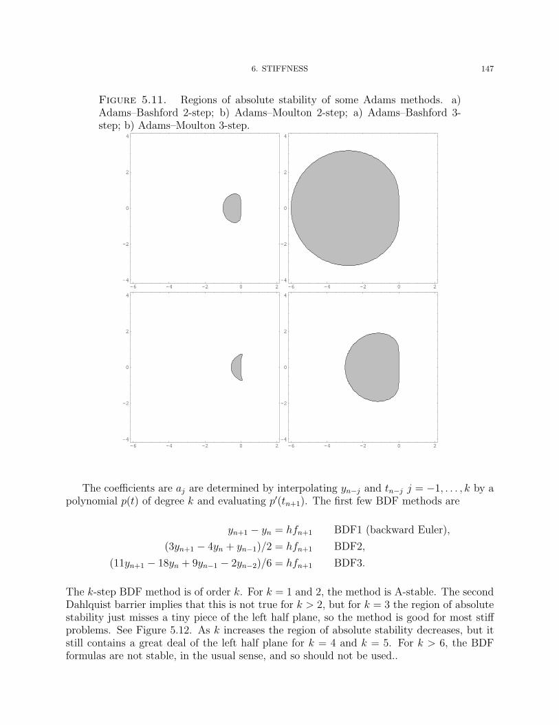
6. STIFFNESS 147
Figure 5.11. Regions of absolute stability of some Adams methods. a)Adams–Bashford 2-step; b) Adams–Moulton 2-step; a) Adams–Bashford 3-step; b) Adams–Moulton 3-step.
-6 -4 -2 0 2-4
-2
0
2
4
-6 -4 -2 0 2-4
-2
0
2
4
-6 -4 -2 0 2-4
-2
0
2
4
-6 -4 -2 0 2-4
-2
0
2
4
The coefficients are aj are determined by interpolating yn−j and tn−j j = −1, . . . , k by apolynomial p(t) of degree k and evaluating p′(tn+1). The first few BDF methods are
yn+1 − yn = hfn+1 BDF1 (backward Euler),
(3yn+1 − 4yn + yn−1)/2 = hfn+1 BDF2,
(11yn+1 − 18yn + 9yn−1 − 2yn−2)/6 = hfn+1 BDF3.
The k-step BDF method is of order k. For k = 1 and 2, the method is A-stable. The secondDahlquist barrier implies that this is not true for k > 2, but for k = 3 the region of absolutestability just misses a tiny piece of the left half plane, so the method is good for most stiffproblems. See Figure 5.12. As k increases the region of absolute stability decreases, but itstill contains a great deal of the left half plane for k = 4 and k = 5. For k > 6, the BDFformulas are not stable, in the usual sense, and so should not be used..

148 5. NUMERICAL SOLUTION OF ORDINARY DIFFERENTIAL EQUATIONS
Figure 5.12. Regions of absolute stability of some BDF methods. a) BDF2-step; b) BDF 3-step; a) BDF 4-step; b) BDF 5-step.
-6 -4 -2 0 2-4
-2
0
2
4
-6 -4 -2 0 2-4
-2
0
2
4
-6 -4 -2 0 2-4
-2
0
2
4
-6 -4 -2 0 2-4
-2
0
2
4
Exercises
(1) Prove that Euler’s method is stable with respect to perturbations in the initial data y0
and the function f . That is, prove that if yn is defined by Euler’s method and yn is definedby the perturbed equations:
yn+1 = yn + hf(tn, yn), y0 given,
then |yn − yn| ≤ C1|y0 − y0|+ C2‖f − f‖L∞(I×R). (State precisely the hypotheses neededand give explicit formulas for C1 and C2.)
(2) State precisely and prove an asymptotic error estimate for the trapezoidal method.
(3) Find the most general two stage Runge–Kutta method of order 2.
(4) For solving the equation y′ = f(t, y), consider the scheme
yn+1 = yn +h
2(y′n + y′n+1) +
h2
12(y′′n − y′′n+1),

EXERCISES 149
where y′n = f(tn, yn), and y′′n = (∂f/∂t + f∂f/∂y)(tn, yn). Determine the order of thismethod. Show that its region of absolute stability contains the entire negative real axis.
(5) Consider a consistent linear multistep methods yn+1 +∑k
j=0 ajyn−j = h∑k
j=−1 bjfn−j
for which the coefficients aj ≤ 0, j = 0, . . . , k (there are many such methods). a) Provethat all such consistent methods satisfy the root condition, and so are stable. b) Give anelementary proof that all such methods are convergent (without invoking the Dahlquisttheory).


CHAPTER 6
Numerical Solution of Partial Differential Equations
1. BVPs for 2nd order elliptic PDEs
We start with a typical physical application of partial differential equations, the modelingof heat flow. Suppose we have a solid body occupying a region Ω ⊂ R3. The temperaturedistribution in the body can be given by a function u : Ω× J → R where J is an interval oftime we are interested in and u(x, t) is the temperature at a point x ∈ Ω at time t ∈ J . Theheat content (the amount of thermal energy) in a subbody D ⊂ Ω is given by
heat content of D =
∫D
cu dx
where c is the product of the specific heat of the material and the density of the material.Since the temperature may vary with time, so can the heat content of D. The rate of changeof heat in D is given by
rate of change of heat in D =∂
∂t
∫D
cu dx =
∫D
∂(cu)
∂t(x, t) dx.
Now any change of heat in D must be accounted for by heat flowing in or out of D throughits boundary or by heat entering from external sources (e.g., if the body were in a microwaveoven). Fourier’s law of heat conduction says that heat flows in the direction opposite thetemperature gradient with a rate proportional to the magnitude of the gradient. That is,the heat flow, at any point and any time, is given by
heat flow = −λ gradu,
where the positive quantity λ is called the conductivity of the material. (Usually λ is justa scalar, but if the material is thermally anisotropic, i.e., it has preferred directions of heatflow, as might be a fibrous or laminated material, λ can be a 3× 3 positive-definite matrix.)Therefore the heat that flows out of D is given by
rate of heat flow out of D = −∫
∂D
(λ gradu) · n ds.
Now the divergence theorem says that for any vectorfield v,∫
∂Dv ·n ds =
∫D
div v dx. Thus
rate of heat flow out of D = −∫
D
div(λ gradu) dx.
Conservation of energy then gives us∫D
∂(cu)
∂tdx−
∫D
div(λ gradu) dx =
∫D
f dx,
151

152 6. NUMERICAL SOLUTION OF PARTIAL DIFFERENTIAL EQUATIONS
where f is the rate at which heat per unit volume is being added from external sources (ifheat is being removed, f is negative). Thus the quantity
∂(cu)
∂t− div(λ gradu)− f
has vanishing integral on any smoothly bounded subregion D. This happens if and only ifthis quantity vanishes. Thus we have derived the equation
∂(cu)
∂t= div(λ gradu) + f in Ω× J.
The source function f , the material coefficients c and λ and the solution u can all be functionsof x and t. If the material is homogeneous (the same everywhere) and not changing withtime, then c and λ are constants and the equation simplifies to the heat equation,
µ∂u
∂t= ∆u+ f ,
where µ = c/λ and we have f = f/λ. If the material coefficients depend on the temperatureu, as may well happen, we get a nonlinear PDE generalizing the heat equation.
The heat equation not only governs heat flow, but all sorts of diffusion processes wheresome quantity flows from regions of higher to lower concentration. The heat equation is theprototypical parabolic differential equation.
Now suppose our body reaches a steady state: the temperature is unchanging. Then thetime derivative term drops and we get
(6.1) − div(λ gradu) = f in Ω,
where now u and f are functions of f alone. For a homogeneous material, this becomes thePoisson equation
−∆u = f ,
the prototypical elliptic differential equation. For an inhomogeneous material we can leavethe steady state heat equation in divergence form as in (6.1), or differentiate out to obtain
−λ∆u+ gradλ · gradu = f.
To determine the steady state temperature distribution in a body we need to know notonly the sources and sinks within the body (given by f), but also what is happening at theboundary Γ := ∂Ω. For example a common situation is that the boundary is held at a giventemperature
(6.2) u = g on Γ.
The PDE (6.1) together with the Dirichlet boundary condition (6.2) form an elliptic bound-ary value problem. Under a wide variety of circumstances this problem can be shown tohave a unique solution. The following theorem is one example (although the smoothnessrequirements can be greatly relaxed).
Theorem 6.1. Let Ω be a smoothly bounded domain in Rn, and let λ : Ω→ R+, f : Ω→R, g : Γ → R be C∞ functions. Then there exists a unique function u ∈ C2(Ω) satisfyingthe differential equation (6.1) and the boundary condition (6.2). Moreover u is C∞.

2. THE FIVE-POINT DISCRETIZATION OF THE LAPLACIAN 153
Instead of the Dirichlet boundary condition of imposed temperature, we often see theNeumann boundary condition of imposed heat flux (flow across the boundary):
∂u
∂n= g on Γ.
For example if g = 0, this says that the boundary is insulated. We may also have a Dirichletcondition on part of the boundary and a Neumann condition on another.
2. The five-point discretization of the Laplacian
With the motivation of the previous section, let us consider the numerical solution of theelliptic boundary value problem
(6.3) ∆u = f in Ω, u = g on Γ.
For simplicity we will consider first a very simple domain Ω = (0, 1)× (0, 1), the unit squarein R2. Now this problem is so simplified that we can attack it analytically, e.g., by separationof variables, but it is very useful to use as a model problem for studying numerical methods.
Let N be a positive integer and set h = 1/N . Consider the mesh in R2
R2h := (mh, nh) : m,n ∈ Z .
Note that each mesh point x ∈ R2h has four nearest neighbors in R2
h, one each to the left,right, above, and below. We let Ωh = Ω∩R2
h, the set of interior mesh points, and we regardthis a discretization of the domain Ω. We also define Γh as the set of mesh points in R2
h
which don’t belong to Ωh, but which have a nearest neighbor in Ωh. We regard Γh as adiscretization of Γ. We also let Ωh := Ωh ∪ Γh
Figure 6.1. Ωh for h = 1/8: • – points in Ωh, – points in Γh.
• • • • • • • • • • • • • • • • • • • • • • • • • • • • • • • • • • • • • • • • • • • • • • • • •
To discretize (6.3) we shall seek a function uh : Ωh → R satisfying
(6.4) ∆h uh = f on Ωh, uh = g on Γh.
Here ∆h is an operator, to be defined, which takes functions on Ωh (mesh functions) tofunctions on Ωh. It should approximate the true Laplacian in the sense that if v is a smoothfunction on Ω and vh = v|Ωh
is the associated mesh function, then we want
∆h vh ≈ ∆ v|Ωh
for h small.
154 6. NUMERICAL SOLUTION OF PARTIAL DIFFERENTIAL EQUATIONS
Before defining ∆h, let us turn to the one-dimensional case. That is, given a function vh
defined at the mesh points nh, n ∈ Z, we want to define a function D2hvh on the mesh points,
so that D2hvh ≈ v′′|Zh if vh = v|Zh. One natural procedure is to construct the quadratic
polynomial p interpolating vh at three consecutive mesh points (n− 1)h, nh, (n+ 1)h, andlet D2
hvh(nh) be the constant value of p′′. This gives the formula
D2hvh(nh) = 2vh[(n− 1)h, nh, (n+ 1)h] =
vh
((n+ 1)h
)− 2vh(nh) + vh
((n− 1)h
)h2
.
D2h is known as the 3-point difference approximation to d2/dx2. We know that if v is C2 in
a neighborhood of nh, then limh→0 v[x − h, x, x + h] = v′′(x)/2. In fact, it is easy to showby Taylor expansion (do it!), that
D2hv(x) = v′′(x) +
h2
12v(4)(ξ), for some ξ ∈
(x− h, x+ h
),
as long as v is C4 near x. Thus D2h is a second order approximation to d2/dx2.
Remark. Alternatively, we could use the Peano kernel theorem to analyze the errorD2
hv(0)− v′′(0), say when h = 1, and then use scaling to get the result for arbitrary h. Weleave this as an exercise for the reader.
Now returning to the definition of the ∆h ≈ ∆ = ∂2/∂x2 + ∂2/∂y2, we simply use the3-point approximation to ∂2/∂x2 and ∂2/∂y2. Writing vm,n for v(mh, nh) we then have
∆h v(mh, nh) =vm+1,n − 2vm,n + vm−1,n
h2+vm,n+1 − 2vm,n + vm,n−1
h2
=vm+1,n + vm−1,n + vm,n+1 + vm,n−1 − 4vm,n
h2.
From the error estimate in the one-dimensional case we easily get that for v ∈ C4(Ω),
∆h v(mh, nh)−∆ v(mh, nh) =h2
12
[∂4v
∂x4(ξ, nh) +
∂4v
∂y4(mh, η)
],
for some ξ, η. Thus:
Theorem 6.2. If v ∈ C2(Ω), then
limh→0‖∆h v −∆ v‖L∞(Ωh) = 0.
If v ∈ C4(Ω), then
‖∆h v −∆ v‖L∞(Ωh) ≤h2
6M4,
where M4 = max(‖∂4v/∂x4‖L∞(Ω), ‖∂4v/∂y4‖L∞(Ω)).
The discrete PDE ∆h uh = f on Ωh is a system of (N − 1)2 linear equations in theunknown values of uh at the mesh points. Since the values of uh are given on the boundarymesh points, we may regard (6.4) as a system of (N − 1)2 linear equations in (N − 1)2

2. THE FIVE-POINT DISCRETIZATION OF THE LAPLACIAN 155
unknowns. For example, in the case N = 4 the system is
−4 1 0 1 0 0 0 0 01 −4 1 0 1 0 0 0 00 1 −4 0 0 1 0 0 01 0 0 −4 1 0 1 0 00 1 0 1 −4 1 0 1 00 0 1 0 1 −4 0 0 10 0 0 1 0 0 −4 1 00 0 0 0 1 0 1 −4 10 0 0 0 0 1 0 1 −4
u1,1
u2,1
u3,1
u1,2
u2,2
u3,2
u1,3
u2,3
u3,3
=
h2f1,1 − u1,0 − u0,1
h2f2,1 − u2,0
h2f3,1 − u3,0 − u4,1
h2f1,2 − u0,2
h2f2,2
h2f3,2 − u4,2
h2f1,3 − u0,3 − u1,4
h2f2,3 − u2,4
h2f3,3 − u4,3 − u3,4
The matrix may be rewritten as A I O
I A IO I A
where I is the 3× 3 identity matrix, O is the 3× 3 zero matrix, and
A =
−4 1 01 −4 10 1 4
.
For general N the matrix can be partitioned into (N − 1) × (N − 1) blocks, each inR(N−1)×(N−1):
A I O · · · O OI A I · · · O OO I A · · · O O...
......
. . ....
...O O O · · · I A
,
where I and O are the identity and zero matrix in R(N−1)×(N−1), respectively, and A ∈R(N−1)×(N−1) is the tridiagonal matrix with −4 on the diagonal and 1 above and below thediagonal. This assumes the unknowns are ordered
u1,1, u2,1, . . . , uN−1,1, u1,2, . . . , uN−1,N−1,
and the equations are ordered similarly.Notice that the matrix has many special properties:
• it is sparse with at most 5 elements per row nonzero• it is block tridiagonal, with tridiagonal and diagonal blocks• it is symmetric• it is diagonally dominant• its diagonal elements are negative, all others nonnegative• it is negative definite
2.1. Analysis via a maximum principle. We will now prove that the problem (6.4)has a unique solution and prove an error estimate. The key will be a discrete maximumprinciple.

156 6. NUMERICAL SOLUTION OF PARTIAL DIFFERENTIAL EQUATIONS
Theorem 6.3 (Discrete Maximum Principle). Let v be a function on Ωh satisfying
∆h u ≥ 0 on Ωh.
Then maxΩhv ≤ maxΓh
v. Equality holds if and only if v is constant.
Proof. Suppose maxΩhv ≥ maxΓh
v. Take x0 ∈ Ωh where the maximum is achieved.Let x1, x2, x3, and x4 be the nearest neighbors. Then
4v(x0) =4∑
i=1
v(xi)− h2 ∆h v(x0) ≤4∑
i=1
v(xi) ≤ 4v(x0),
since v(xi) ≤ v(x0). Thus equality holds throughout and v achieves its maximum at all thenearest neighbors of x0 as well. Applying the same argument to the neighbors in the interior,and then to their neighbors, etc., we conclude that v is constant.
Remarks. 1. The analogous discrete minimum principle, obtained by reversing the in-equalities and replacing max by min, holds. 2. This is a discrete analogue of the maximumprinciple for the Laplace operator.
Theorem 6.4. There is a unique solution to the discrete boundary value problem (6.4).
Proof. Since we are dealing with a square linear system, it suffices to show nonsingu-larity, i.e., that if ∆h uh = 0 on Ωh and uh = 0 on Γh, then uh ≡ 0. Using the discretemaximum and the discrete minimum principles, we see that in this case uh is everywhere0.
The next result is a statement of maximum norm stability.
Theorem 6.5. The solution uh to (6.4) satisfies
(6.5) ‖uh‖L∞(Ωh) ≤1
8‖f‖L∞(Ωh) + ‖g‖L∞(Γh).
This is a stability result in the sense that it states that the mapping (f, g) 7→ uh isbounded uniformly with respect to h.
Proof. We introduce the comparison function φ = [(x − 1/2)2 + (y − 1/2)2]/4, whichsatisfies ∆h φ = 1 on Ωh, and 0 ≤ φ ≤ 1/8 on Ωh. Set M = ‖f‖L∞(Ωh). Then
∆h(uh +Mφ) = ∆h uh +M ≥ 0,
so
maxΩh
uh ≤ maxΩh
(uh +Mφ) ≤ maxΓh
(uh +Mφ) ≤ maxΓh
g +1
8M.
Thus uh is bounded above by the right-hand side of (6.5). A similar argument applies to−uh giving the theorem.
By applying the stability result to the error u − uh we can bound the error in terms ofthe consistency error ∆h u−∆u.
Theorem 6.6. Let u be the solution of the Dirichlet problem (6.1) and uh the solutionof the discrete problem (6.4). Then
‖u− uh‖L∞(Ωh) ≤1
8‖∆u−∆h u‖L∞(Ωh).

2. THE FIVE-POINT DISCRETIZATION OF THE LAPLACIAN 157
Proof. Since ∆h uh = f = ∆u on Ωh, ∆h(u − uh) = ∆h u −∆u. Also, u − uh = 0 onΓh. Apply Theorem 6.5 (with uh replaced by u− uh), we obtain the theorem.
Combining with Theorem 6.2, we obtain error estimates.
Corollary 6.7. If u ∈ C2(Ω), then
limh→0‖u− uh‖L∞(Ωh) = 0.
If u ∈ C4(Ω), then
‖u− uh‖L∞(Ωh) ≤h2
48M4,
where M4 = max(‖∂4u/∂x4‖L∞(Ω), ‖∂4u/∂y4‖L∞(Ω)).
Remark. The quantity ‖∆u−∆h u‖ is the consistency error of the discretization, andthe statement that limh→0‖∆u−∆h u‖ = 0 means that the discretization is consistent. Anestimate of the form ‖v‖ ≤ Ch‖f‖ whenever ∆h v = f on Ωh and v = 0 on Γh, is a stabilityestimate, and if it holds with Ch independent of h, we say the discretization is stable. Thepreceding proof shows that
consistency + stability =⇒ convergence.
(Of course all three concepts are defined with respect to specific norms.)
2.2. Fourier analysis. Define L(Ωh) to be the set of functions Ωh → R, which isisomorphic to RM , M = (N −1)2. Sometimes we think of these as functions on Ωh extendedby zero to Γh. The discrete Laplacian then defines an isomorphism of L(Ωh) onto itself. Thestability result from the previous section says simply that ‖∆−1
h ‖ ≤ 1/8 where the operatornorm is with respect to the L∞ norm on L(Ωh). In this section we use Fourier analysis toestablish a similar stability result for a discrete analogue of the L2 norm.
First consider the one-dimensional case. With h = 1/N let Ih = h, 2h, . . . , (N − 1)h,and let L(Ih) be the space of functions on Ih, which is an N − 1 dimensional vectorspace.On L(Ih) we define the inner product
〈u, v〉h = hN−1∑k=1
u(kh)v(kh),
with the corresponding norm ‖v‖h.The space L(Ih) is a discrete analogue of L2(I) where I is the unit interval. On this
latter space the functions sin πmx, m = 1, 2, . . ., form an orthogonal basis consisting ofeigenfunctions of the operator d2/dx2. The corresponding eigenvalues are π2, 4π2, 9π2, . . ..We now establish the discrete analogue of this result.
Define φm ∈ L(Ih) by φm(x) = sin πmx, x ∈ Ih. It turns out that these mesh functionsare precisely the eigenvectors of the operator D2
h. Indeed
D2hφm(x) =
sin πm(x+ h)− 2 sin πmx+ sin πm(x− h)h2
=2
h2(cosπmh− 1) sin πmx.
Thus
D2hφm = −λmφm, λm =
2
h2(1− cos πmh) =
4
h2sin2 πmh
2.

158 6. NUMERICAL SOLUTION OF PARTIAL DIFFERENTIAL EQUATIONS
Note that
0 < λ1 < λ2 < · · · < λN−1 <4
h2.
Note also that for small m << N , λm ≈ π2m2. In particular λ1 ≈ π2. To get a strict lowerbound we note that λ1 = 8 for N = 2 and λ1 increases with N .
Since the operator D2h is symmetric with respect to the inner product on L(Ih), and the
eigenvalues λm are distinct, it follows that the eigenvectors φm are mutually orthogonal. (Thiscan also be obtained using trigonometric identities, or by expressing the sin functions in termsof complex exponentials and using the discrete Fourier transform studied in Chapter 1.7.)Since there are N − 1 of them, they form a basis of L(Ih).
Theorem 6.8. The functions φm, m = 1, 2, . . . , N − 1 form an orthogonal basis ofL(Ih). Consequently, any function v ∈ L(Ih) can be expanded as v =
∑N−1m=1 amφm with
am = 〈v, φm〉h/‖φm‖2h, and ‖v‖2h =∑N−1
m=1 a2m‖φm‖2h.
From this we obtain immediately a stability result for the one-dimensional Laplacian. Ifv ∈ L(Ih) and D2
hv = f , we expand v in terms of the φm:
v =N−1∑m=1
amφm, ‖v‖2h =N−1∑m=1
a2m‖φm‖2h.
Then
f = −N−1∑m=1
λmamφm, ‖f‖2h =N−1∑m=1
λ2ma
2m‖φm‖2h ≥ 82‖v‖2h.
Thus ‖v‖h ≤ ‖f‖h/8.
The extension to the two-dimensional case is straightforward. We use the basis φmn =φm ⊗ φn, i.e.,
φmn(x, y) := φm(x)φn(y), m, n = 1, . . . , N − 1,
for L(Ωh). It is easy to see that these (N − 1)2 functions form an orthogonal basis for L(Ωh)equipped with the inner product
〈u, v〉h = h2
N−1∑m=1
N−1∑n=1
u(mh, nh)v(mh, nh)
and corresponding norm ‖ · ‖h. Moreover φmn is an eigenvector of ∆h with eigenvalue λmn =λm + λn ≥ 16. The next theorem follows immediately.
Theorem 6.9. The operator ∆h defines an isomorphism from L(Ωh) to itself. Moreover‖∆−1
h ‖ ≤ 1/16 where the operator norm is with respect to the norm ‖ · ‖h on L(Ωh).
Since the ‖v‖h ≤ ‖v‖L∞(Ωh) we also have consistency with respect to the discrete 2-norm.We leave it to the reader to complete the analysis with a convergence result.

2. THE FIVE-POINT DISCRETIZATION OF THE LAPLACIAN 159
2.3. Analysis via an energy estimate. Let v be a mesh function. Define the back-ward difference operator
∂xv(mh, nh) =v(mh, nh)− v((m− 1)h, nh)
h, 1 ≤ m ≤ N, 0 ≤ n ≤ N.
In this section we denote
〈v, w〉h = h2
N∑m=1
N∑n=1
v(mh, nh)w(mh, nh),
with the corresponding norm ‖ · ‖h (this agrees with the notation in the last section for meshfunctions which vanish on Γh).
Lemma 6.10. If v ∈ L(Ωh) (the set of mesh functions vanishing on Γh), then
‖v‖h ≤ ‖∂xv‖h.
Proof. For 1 ≤ m ≤ N , 0 ≤ n ≤ N ,
|v(mh, nh)|2 ≤
(N∑
i=1
|v(ih, nh)− v((i− 1)h, nh)|
)2
=
(h
N∑i=1
|∂xv(ih, nh)|
)2
≤
(h
N∑i=1
|∂xv(ih, nh)|2)(
hN∑
i=1
12
)
= hN∑
i=1
|∂xv(ih, nh)|2.
Therefore
h
N∑m=1
|v(mh, nh)|2 ≤ h
N∑i=1
|∂xv(ih, nh)|2
and
h2
N∑m=1
N∑n=1
|v(mh, nh)|2 ≤ h2
N∑i=1
N∑n=1
|∂xv(ih, nh)|2.
This result is a discrete analogue of Poincare’s inequality, which bounds a function interms of its gradient as long as the function vanishes on a portion of the boundary. Theimplied constant of 1 in the bound can be improved. The next result is a discrete analogueof Green’s Theorem (essentially, integration by parts).
Lemma 6.11. If v, w ∈ L(Ωh), then
−〈∆h v, w〉h = 〈∂xv, ∂xw〉h + 〈∂yv, ∂yw〉h.

160 6. NUMERICAL SOLUTION OF PARTIAL DIFFERENTIAL EQUATIONS
Proof. Let v0, v1, . . . , vN , w0, w1, . . . , wN ∈ R with w0 = wN = 0. Then
N∑i=1
(vi − vi−1)(wi − wi−1) =N∑
i=1
viwi +N∑
i=1
vi−1wi−1 −N∑
i=1
vi−1wi −N∑
i=1
viwi−1
= 2N−1∑i=1
viwi −N−1∑i=1
vi−1wi −N−1∑i=1
vi+1wi
= −N−1∑i=1
(vi+1 − 2vi + vi−1)wi.
Hence,
− hN−1∑i=1
v((i+ 1)h, nh)− 2v(ih, nh) + v((i− 1)h, nh)
h2w(ih, nh)
= hN∑
i=1
∂xv(ih, nh)∂xw(ih, nh),
and thus−〈D2
xv, w〉h = 〈∂xv, ∂xw〉h.Similarly, −〈D2
yv, w〉h = 〈∂yv, ∂yw〉h, so the lemma follows.
Combining the discrete Poincare inequality with the discrete Green’s theorem, we imme-diately get a stability result. If v ∈ L(Ωh), then
‖v‖2h ≤ ‖∂xv‖2h ≤ ‖∂xv‖2h + ‖∂yv‖2h = −〈∆h v, v〉h ≤ ‖∆h v‖h‖v‖h.Thus
‖v‖h ≤ ‖∆h v‖h, v ∈ L(Ωh),
which is a stability result.
2.4. Curved boundaries. Thus far we have studied as a model problem the discretiza-tion of Poisson’s problem on the square. In this subsection we consider a variant which canbe used to discretize Poisson’s problem on a fairly general domain.
Let Ω be a smoothly bounded open set in R2 with boundary Γ. We again consider theDirichlet problem for Poisson’s equation, (6.3), and again set Ωh = Ω ∩ R2
h. If (x, y) ∈ Ωh
and the segment (x+ sh, y), 0 ≤ s ≤ 1 belongs to Γ, then the point (x+h, y), which belongsto Ωh, is a neighbor of (x, y) to the right. If this segment doesn’t belong to Ω we defineanother sort of neighbor to the right, which belongs to Γ. Namely we define the neighbor tobe the point (x + sh, y) where 0 < s ≤ 1 is the largest value for which (x + th, y) ∈ Ω forall 0 ≤ t < s. The points of Γ so constructed (as neighbors to the right or left or above orbelow points in Ωh) constitute Γh. Thus every point in Ωh has four nearest neighbors all of
which belong to Ωh := Ωh ∪ Γh. We also define Ωh as those points in Ωh all four of whoseneighbor belong to Ωh. See Figure 6.2.
In order to discretize the Poisson equation we need to construct a discrete analogue ofthe Laplacian ∆h v for mesh functions v on Ωh. Of course on Ωh, ∆h v is defined as theusual 5-point Laplacian. For (x, y) ∈ Ωh \ Ωh, let (x + h1, y), (x, y + h2), (x − h3, y), and

2. THE FIVE-POINT DISCRETIZATION OF THE LAPLACIAN 161
Figure 6.2. The dots are points in Ωh with the elements of Ωh being circled.The triangles are the points of Γh.
(x, y − h4) be the nearest neighbors (with 0 < hi ≤ h), and let v1, v2, v3, and v4 denotethe value of v at these four points. Setting v0 = v(x, y) as well, we will define ∆h v(x, y) asa linear combination of the five values vi. In order to derive the formula, we first considerapproximating d2v/dx2(0) by a linear combination of v(−h−), v(0), and v(h+), for a functionv of one variable. By Taylor’s theorem
α−v(−h−) + α0v(0) + α+v(h+) = (α− + α0 + α+)v(0) + (α+h+ − α−h−)v′(0)
+1
2(α+h
2+ + α−h
2−)v′′(0) +
1
6(α+h
3+ − α−h3
−)v′′′(0) + · · · .
Thus, to obtain a consistent approximation we must have
α− + α0 + α+ = 0, α+h+ − α−h− = 0,1
2(α+h
2+ + α−h
2−) = 1,
which give
α− =2
h−(h− + h+), α+ =
2
h+(h− + h+), α0 =
−2
h−h+
.
Note that we have simply recovered the usual divided difference approximation to d2v/dx2:
α−v(−h−)+α0v(0)+α+v(h+) =[v(h+)− v(0)]/h+ − [v(0)− v(−h−)]/h−
(h+ + h−)/2= 2v[−h−, 0, h+].
Returning to the 2-dimensional case, and applying the above considerations to both∂2v/∂x2 and ∂2v/∂y2 we arrive at the Shortley–Weller formula for ∆h v:
∆h v(x, y)
=2
h1(h1 + h3)v1 +
2
h2(h2 + h4)v2 +
2
h3(h1 + h3)v3 +
2
h4(h2 + h4)v4 −
(2
h1h3+
2
h2h4
)v0.
Using Taylor’s theorem with remainder we easily calculate that for v ∈ C3(Ω),
‖∆ v −∆h v‖L∞(Ωh) ≤2M3
3h,

162 6. NUMERICAL SOLUTION OF PARTIAL DIFFERENTIAL EQUATIONS
where M3 is the maximum of the L∞ norms of the third derivatives of v. Of course at themesh points in Ωh, the truncation error is actually O(h2), but for mesh points neighboringthe boundary, it is reduced to O(h).
The approximate solution to (6.3) is uh : Ωh → R determined again by 6.4. This is asystem of linear equations with one unknown for each point of Ωh. In general the matrixwon’t be symmetric, but it maintains other good properties from the case of the square:
• it is sparse, with at most five elements per row• it has negative diagonal elements and non-negative off-diagonal elements• it is diagonally dominant.
Using these properties we can obtain the discrete maximum principle with virtually the sameproof as for Theorem 6.3, and then a stability result as in Theorem 6.5 follows as before. Inthis way we can easily obtain an O(h) convergence result.
In fact this result can be improved. Although the truncation error ‖∆u − ∆h u‖L∞(Ωh)
is only O(h), it is O(h2) at all points except those neighboring the boundary, and theseaccount for only O(h−1) of the O(h−2) points in Ωh. Moreover these points are within h ofthe boundary, where the solution is known exactly. For both of these reasons the contributionto the error from these points is smaller than is seen from the simple argument outlined inthe previous paragraph. A sharp convergence result was proven by Bramble and Hubbardin a paper in Numerische Mathematik 4 (1962), pp. 313–327.
Theorem 6.12. Let u be the solution to (6.3) and let uh be the mesh function satisfying(6.4). Then
‖u− uh‖L∞(Ωh) ≤M4d
2
96h2 +
2M3
3h3,
where d is the diameter of the smallest disk containing Ω and Mk = maxi+j=k
‖∂ku/∂xi∂yj‖∞.
Thus the rate of convergence is O(h2) as in the case of the square, and the points nearthe boundary contribute only a higher order term (despite the fact that the truncation erroris of lower order there).
3. Finite element methods
3.1. The weak formulation of the Dirichlet problem. We start by consideringPoisson’s equation with homogeneous Dirichlet boundary conditions on a bounded planedomain Ω:
(6.6) ∆u = f in Ω, u = 0 on Γ.
Let’s assume that f is continuous on Ω. Now if we multiply the differential equation by atest function v and integrate over Ω, we get that∫
Ω
∆u v dx =
∫Ω
fv dx,
and conversely, if this equation is satisfied for all integrable functions v, then u satisfiesPoisson’s equation. In fact, it is sufficient that the equation be satisfied for all C∞ functions
3. FINITE ELEMENT METHODS 163
with compact support inside Ω. In particular, if v is a C1 function on Ω which vanishes onΓ, we may integrate by parts to get
(6.7)
∫Ω
gradu · grad v dx = −∫
Ω
fv dx.
Thus it is evident that a C2 function which vanishes on Γ satisfies Poisson’s equation if andonly if it satisfies (6.7) for all C2 functions v which vanish on Γ. The use of C2 functionsis, however, not very natural for the formulation (6.7). A more natural space would be theSobolev space
H1(Ω) = v ∈ L2(Ω) |∇v ∈ L2(Ω) .This is a Hilbert space with inner product
〈u, v〉H1(Ω) =
∫Ω
(uv + gradu · grad v) dx,
and corresponding norm
‖v‖1 = ‖v‖H1(Ω) :=√‖v‖2L2(Ω) + ‖grad v‖2L2(Ω).
(Note: we are using the same notation L2(Ω) both for real-valued and vector-valued squareintegrable functions.) We also define
H1(Ω) = v ∈ H1(Ω) | v|Γ ≡ 0 .We then define the weak formulation of the Dirichlet problem for Poisson’s equation to be:
Find u ∈ H1(Ω) such that
(6.8)
∫Ω
gradu · grad v dx = −∫
Ω
fv dx for all v ∈ H1(Ω).
The weak formulation fits an abstract framework we shall see frequently. We have a Hilbertspace V (namely H1(Ω)), a bilinear form B : V × V → R (given by the left-hand side of(6.8)), a linear functional F : V → R (given by the right-hand side of (6.8)), and the weakformulation is
(6.9) Find u ∈ V such that B(u, v) = F (v) for all v ∈ V .
It is clear that if u is a C2 function satisfying the classical formulation (6.6) of our bound-
ary value problem, then u ∈ H1(Ω) and u satisfies the weak formulation (6.8). Conversely, ifu solves the weak formulation, and if u is C2, then u is a classical solution to the boundaryvalue problem. However the classical formulation and the weak formulation are not entirelyequivalent, because it may happen that there is a solution to the weak formulation which isnot C2. It can be shown that a solution to the weak formulation is automatically smooth ifboth the forcing function f is smooth and the domain Ω has a smooth boundary, but suchelliptic regularity theorems are not trivial.
Remark. In defining the Sobolev spaces H1(Ω) and H1(Ω) we have glossed over severalpoints. In the definition of the former space, we assumed that it is clear what is meant bygrad v when v ∈ L2(Ω). If the reader is familiar with the theory of distributions, this is noproblem: she then knows that grad v in any case exists as a distribution, which may, or maynot, then belong to L2. Briefly, given an L2 function v, a vector-valued L2 function w is

164 6. NUMERICAL SOLUTION OF PARTIAL DIFFERENTIAL EQUATIONS
equal to grad v if and only if∫
Ωv div φ dx = −
∫Ωw ·φ dx for all C∞ vector-valued functions φ
with compact support in Ω. A more subtle point is that in defining H1(Ω), we have assumedthat it is clear what is meant by v|Γ for v ∈ H1(Ω). This is not so evident. For example,there is certainly no way to make sense of v|Γ for an arbitrary function v ∈ L2(Ω) (whichis defined only almost everywhere, and may not be defined anywhere on Γ). In fact, it canbe shown that there is a unique bounded map γ : H1(Ω) → L2(Γ) such that γv = v|Γ forall v ∈ H1(Ω) ∪ C(Ω). This is an example of a trace theorem, and requires some effort toestablish. By v|Γ we simply mean γv, for any v ∈ H1(Ω).
The weak formulation is in many ways a very natural formulation of the Dirichlet problemfor Poisson’s equation. One indication of this is that it is quite simple to establish existenceand uniqueness of weak solutions. One first establishes Poincare’s inequality, which statesthat there exists a constant c depending only on the domain Ω such that ‖u‖L2(Ω) ≤ c‖u‖H1(Ω)
for all u ∈ H1(Ω). This is fairly elementary; a good exercise is to prove it in the one-dimensional case where Ω is a bounded interval (what is the best constant c?). It follows
that on the space H1(Ω), the quantity√‖gradu‖L2 is a norm equivalent to the full H1 norm,
and hence the left-hand side of (6.8) defines an inner product on H1(Ω) which is equivalentto the H1 inner product. Existence and uniqueness of a weak solution is then an immediateconsequence of the Riesz representation theorem.
Remark. Besides the weak formulation of the boundary value problem (6.6), there is
a closely related variational formulation. In this we seek u ∈ H1(Ω) which minimizes theenergy functional
E(w) :=1
2
∫Ω
| gradw|2 dx+
∫Ω
fw dx
over w ∈ H1(Ω). If u is the solution of the weak formulation and w ∈ H1(Ω) with w 6= u
but otherwise arbitrary, we may write w = u+ v, with 0 6= v ∈ H1(Ω), and then
E(w) =1
2
∫Ω
| gradu|2 dx+
∫Ω
gradu · grad v dx+1
2
∫Ω
| grad v|2 dx+
∫Ω
fu dx+
∫Ω
fv dx
= E(u) +
[∫Ω
gradu · grad v dx+
∫Ω
fv dx
]+
1
2
∫Ω
| grad v|2 dx.
The term in brackets vanishes since u is the weak solution, and the final term is positive ifv 6= 0. Thus E(u) < E(w), and u is indeed the minimizer. Conversely, if u minimizes E over
H1(Ω) and v ∈ H1(Ω) is arbitrary, then the quadratic function G : R→ R given by
G(t) = E(u+ tv) = E(u) + t
[∫Ω
gradu · grad v dx+
∫Ω
fv dx
]+t2
2
∫Ω
| grad v|2 dx,
has its minimum at t = 0, and this immediately shows that u is a weak solution. Thus thenotion of a weak solution and a variational solution (a minimizer of the energy functional)are equivalent for this problem. For problems which are not symmetric however (e.g., if thePDE were ∆u + ∂u/∂x = f), there is no natural variational formulation, while the weakformulation still applies.

3. FINITE ELEMENT METHODS 165
3.2. Galerkin’s method. In the weak formulation, we seek a function in the trial spaceH1(Ω) which satisfies the weak equation (6.8) for all v in the test space H1(Ω). In Galerkin’s
method we choose a finite dimensional space Sh ⊂ H1(Ω), and use it in place of H1(Ω) astrial and test space. That is, we seek uh ∈ Sh satisfying the discrete weak formulation∫
Ω
graduh · grad v dx = −∫
Ω
fv dx for all v ∈ Sh.
Let us show that such a function uh exists and is unique. Let φ1, . . . , φN be any basis of
Sh. Then we are seeking uh =∑N
j=1 αjφj such that∫Ω
graduh · gradφi dx = −∫
Ω
fφi dx, i = 1, . . . , N.
(By linearity, it is enough that the weak equation hold for each basis function.) This meansthat
N∑j=1
αj
∫Ω
gradφj · gradφi dx = −∫
Ω
fφi dx.
If we define the stiffness matrix M ∈ RN×N by
Mij =
∫Ω
gradφj · gradφi dx,
and the load vector F ∈ RN by
Fi = −∫
Ω
fφi dx,
then the coefficient vector α is determined as the solution of the linear system
Mα = F .
The matrix M is clearly symmetric, and it is positive definite as well, since for any vectorα ∈ RN ,
αTMα =∑ij
αiαj
∫Ω
gradφj · gradφi dx
=
∫Ω
grad
(∑j
αjφj
)· grad
(∑i
αiφi
)dx =
∫Ω
| grad v|2 dx,
where v =∑
j αjφj. Since the latter quantity is a norm of v it is positive unless v ≡ 0 whichonly happens if α = 0.
Thus Galerkin’s method is implementable. If we choose a space Sh for which we can finda basis which is not too complicated, we can compute the N2 integrals giving the stiffnessmatrix and the N integrals giving the load vector, and then solve the resulting N × Nsymmetric positive definite linear system to find the coefficients of uh with respect to thebasis.
Remark. Instead of beginning with the weak formulation and restricting the test andtrial spaces to a finite dimensional subspace, we may start with the variational formulationand restrict the trial space to Sh. That is, we define uh ∈ Sh to be the minimizer of E(v) over

166 6. NUMERICAL SOLUTION OF PARTIAL DIFFERENTIAL EQUATIONS
v ∈ Sh. This is called the Ritz method. Following the proof for the continuous case we seethat uh is in fact just the Galerkin solution. This viewpoint, that the approximate solutionis determined by restricting the minimization of energy to a finite dimensional space, wasthe first motivation for the finite element method. However, we obtain greater generality byusing the weak formulation and Galerkin’s method rather than the variational formulationand the Ritz method.
3.3. A simple finite element method. The finite element method consists of theGalerkin method together with the choice of a particular sort of subspace Sh. Namely wepartition Ω into a finite number of disjoint triangles or other simple pieces, and take Sh tobe a space of piecewise polynomials with respect to this partition.
More specifically, let us assume, for now, that Ω is a polygon. Given a triangulation Th
we define M10 (Th) to be the space of continuous piecewise linear functions subordinate to this
triangulation, that is the space of continuous functions on Ω which restrict to polynomials ofdegree at most 1 on each T ∈ Th. The notation is the same as in Chapter 1.5: the superscript1 refers to the polynomial degree and the subscript 0 to the fact that the continuity of C0
is enforced. It is easy to check that a piecewise polynomial is in H1 if and only if it iscontinuous: the gradient of a continuous piecewise polynomial is the L2 function obtainedby taking the gradient triangle by triangle. Thus for any triangulation, M1
0 (Th) is a subspace
of H1. As a subspace of H1, we then take
Sh = M10 (Th) = M1
0 (Th) ∩ H1(Ω).
This is the simplest finite element space for the Dirichlet problem. A basis for Sh is givenby the hat functions associated with all the interior vertices.
Recall that the hat functions are local basis functions in that each is supported on justa few triangles. Namely, the support of φj is the union of the triangles sharing the vertexxj), and there will only be a few other basis functions whose support contains one of thesetriangles, namely the basis functions associated to vertices of triangles in the support of φj.If φi is any other basis function, then the corresponding stiffness matrix entry∫
gradφj · gradφi dx = 0.
As a consequence we see that with the hat function basis, the stiffness matrix is very sparse(there will be only a few nonzero entries per row, and this number will not increase when werefine the mesh, as long as we don’t allow the triangle angles to decrease). Also the stiffnessmatrix entries which are nonzero are nonetheless easily computed: they are sums of integralsof polynomials over only a few triangles (in fact, except for the diagonal entries of the stiffnessmatrix, over two triangles). This adds greatly to the efficiency of the implementation of theGalerkin method.
We may now roughly define the finite element method: it is Galerkin’s method using apiecewise polynomial trial space with a local basis.
Let us now work out a simple example. We take Ω to be the unit square with a uniformmesh. Namely we divide Ω into n × n subsquares of size h = 1/n and divide each of theseinto two triangles using the positively sloped diagonal. See Figure 6.3.
Now if φ is a linear function, then ∂φ/∂x is constant, and we can find it by evaluating φat any two distinct points on a horizontal line, and taking a difference quotient. Since each

3. FINITE ELEMENT METHODS 167
Figure 6.3. Uniform mesh of the square.
of our triangles has a horizontal and a vertical edge, and since we know the values of thehat basis functions at the vertices, we can easily compute the partial derivatives of the basisfunctions. These are shown in the following figure.
Figure 6.4. Values of ∂φ/∂x and ∂φ/∂y for a hat function.
0
1/h
1/h
-1/h
-1/h
01/h
-1/h
-1/h
1/h0
0
It is then easy to compute the stiffness matrix. Writing φij for the basis function associ-ated to the vertex xij = (ih, jh), we find∫
gradφij · gradφkl dx =
4, i = k, j = l,
−1, i = k ± 1, j = l or i = k, j = l ± 1,
0, else.
In other words, the stiffness matrix for piecewise linear finite elements for the Laplace opera-tor on the unit square using a uniform mesh is exactly the matrix of the five-point Laplacian.If we set
fij :=1
h2
∫fφij.
and write the finite element solution as uh =∑
i,j Uijφij, we have
4Uij − Ui+1,j − Ui−1,j − Ui,j+1 − Ui,j−1
h2+ fij = 0.

168 6. NUMERICAL SOLUTION OF PARTIAL DIFFERENTIAL EQUATIONS
Note that∫φij dx = h2 and if f is at least C2, then fij = f(xij) +O(h2).
From this fact and our earlier analysis of the five-point Laplacian, it is easy to derivean O(h2) convergence estimate at the vertices. In fact, as we shall see, one of the greatstrengths of the finite element method is that there is a very natural approach to the erroranalysis (which does not involve relating it to finite difference methods). The most naturalestimates are obtained in H1(Ω) and L2(Ω) (error estimates in L∞(Ω) can also be obtained,but are more complicated). Below we shall prove, in more general circumstances, that if thesolution u ∈ H2(Ω), then
‖u− uh‖H1(Ω) ≤ Ch‖u‖H2(Ω), ‖u− uh‖L2(Ω) ≤ Ch2‖u‖H2(Ω),
for some constant C. Note that unlike our finite difference estimates the norms are norms offunctions on Ω, not just at the mesh vertices. Note also that we only require that u ∈ H2,not even C2, to obtain O(h2) convergence. By contrast in the finite difference case we neededu ∈ C4. For example, if the function f is merely in L2, then it may not even be defined atthe mesh points, and the standard finite difference method is not meaningful, while the finiteelement method is applicable and will still deliver second order convergence in this case.
Most important, the same error estimates hold on a quite arbitrary domain with anarbitrary triangulation. In this case h is to be interpreted as the diameter of the largesttriangle in the triangulation. The constant C in the estimates will depend on the domain,but not on the triangulation (except that we will need to enforce a bound on the smallestangle of a triangle). The derivation of such error estimates will be discussed later. The pointto note now is the power and flexibility of the finite element method in providing secondorder convergent schemes on unstructured meshes. If we were to try to derive such schemesdirectly, e.g., by Taylor expansions, it would be very messy indeed.
3.4. Application to more general problems. Another great strength of finite ele-ment methods is the ease with which they can be adapted to a wide variety of problems.
3.4.1. More general elliptic PDEs. For example, suppose we replace Poisson’s equation∆u = f with a more general second order PDE
2∑i,j=1
∂
∂xi
(aij
∂u
∂xj
)+
2∑i=1
bi∂u
∂xi
+ cu = f.
Here the coefficients aij, bi, and c may be functions of x. Once again, we may multiply by a
test function v ∈ H1(Ω) and integrate over Ω by parts to obtain a weak formulation of theDirichlet problem in the form (6.9). The only difference is that now
B(u, v) =
∫Ω
∑i,j
aij∂u
∂xj
∂v
∂xi
−∑
i
bi∂u
∂xi
v − cuv dx.
Restricting the trial and test functions to Sh, we obtain a finite element method as before.If the PDE is elliptic, which means that the matrix aij(x) is symmetric positive-definite,uniformly in x, then the behavior of the finite element method for this problem will be verysimilar to that for the Poisson problem. Thus the finite element method is well able tohandle variable coefficients, anisotropic equations, and lower order terms.
We can even allow the coefficients to depend on the solution u, and so have a nonlinearPDE. In that case the form B(u, v) will be linear in v but nonlinear in u. Again the finite

3. FINITE ELEMENT METHODS 169
element method can be applied, although of course the resulting system of algebraic equationswill be nonlinear.
3.4.2. Neumann boundary conditions. Yet another great strength of finite element meth-ods is their flexibility in handling different boundary conditions (which can be very trickyfor finite difference methods). Consider for example Poisson’s equation on a polygon butsuppose that some sides are subject to the Dirichlet boundary condition u = 0 and some tothe Neumann boundary condition, so the problem is to find u satisfying
∆u = f in Ω, u = 0 on ΓD,∂u
∂n= 0 on ΓN ,
where ΓD and ΓN are disjoint open subsets of Γ such that Γ = ΓD ∪ ΓN . The first thing youmight think to do is to seek u in a subspace of H1(Ω) satisfying both boundary conditions,i.e., in
v ∈ H1(Ω) | v|ΓD≡ 0, ∂v/∂n|ΓN
≡ 0 .However, this does not work, because there is no way to define ∂v/∂n for v ∈ H1. Such afunction has a well defined restriction to Γ (or ΓD) but its first derivatives, which are merelyL2 functions, do not. To see our way around this problem, let us multiply Poisson’s equationby a smooth test function v and integrate over Ω.
Green’s formula for integration by parts shows us the way around this difficulty. For anysmooth u and v we have∫
Ω
gradu · grad v dx = −∫
Ω
∆u v dx+
∫Γ
∂u
∂nv ds.
If u satisfies Poisson’s equation, then∫Ω
∆u v dx =
∫Ω
f v dx,
and if u satisfies the Neumann boundary condition, then∫Γ
∂u
∂nv ds =
∫ΓD
∂u
∂nv ds.
DefineH1
D(Ω) = v ∈ H1(Ω) | v|ΓD≡ 0 .
Note that in this space the Dirichlet boundary condition has been imposed, but the Neumannboundary condition has been ignored (since there is no way to make sense of it in H1). Thisleads us to the weak formulation for the mixed Dirichlet/Neumann boundary value problem:Find u ∈ H1
D(Ω) such that∫Ω
gradu · grad v dx = −∫
Ω
f v dx for all v ∈ H1D(Ω).
Just as for the pure Dirichlet problem, as an easy consequence of the Riesz representationtheorem and the Poincare inequality, this problem has a unique solution.
In deriving the weak formulation, we have shown that if u is a classical solution to theboundary value problem then it satisfies this weak formulation. Conversely, if u solves theweakly formulated problem, and u is C2, then we can integrate by parts to find that
−∫
Ω
∆u v dx+
∫Γ
∂u
∂nv ds = −
∫Ω
f v dx for all v ∈ H1D(Ω).

170 6. NUMERICAL SOLUTION OF PARTIAL DIFFERENTIAL EQUATIONS
Taking first v to be smooth and compactly supported in Ω, we conclude that ∆u = f in Ω.Therefore ∫
Γ
∂u
∂nv ds = 0
for all v ∈ H1D(Ω). Since such a function can be arbitrary on ΓN , we conclude that ∂u/∂n = 0
on ΓN .To summarize: the weak formulation for the mixed Dirichlet/Neumann boundary value
problem has a unique solution. This coincides with the classical solution whenever it is C2
and whenever a classical solution exists. Note that the Dirichlet and Neumann boundaryconditions are treated completely differently in the weak formulation. The Dirichlet conditionis imposed a priori by building it into the trial space. The Neumann condition is not builtinto the trial space, but arises as a consequence of the weak formulation. The terminologyused for this is that the Dirichlet condition is an essential boundary condition, while theNeumann condition is natural.
Once we have the weak formulation we can use Galerkin’s method with any subspaceSh of H1
D(Ω). This leads to a symmetric positive definite matrix problem. As long as wearrange that each triangle edge in the boundary belongs entirely to either ΓD or ΓN we caneasily construct a piecewise linear finite element space:
M10D(Th) = M1
0 (Th) ∩H1D(Ω).
A local basis is given by the hat functions at all the triangulation vertices except thosebelonging to ΓD.
We didn’t consider the case of pure Neumann conditions because the boundary valueproblem ∆u = f in Ω, ∂u/∂n = 0 on Γ is not well-posed. Green’s theorem implies thatthere is no solution unless
∫Ωf = 0, and if there is a solution, we can add any constant to it
to get another solution. If we consider instead the differential equation −∆u + u = f , or,more generally, − div(A gradu) + cu = f where A is a symmetric positive definite matrixand c > 0, this problem goes away and the considerations above apply equally well to thepure Neumann problem (ΓN = Γ, ΓD = ∅).
3.4.3. Inhomogeneous boundary conditions. Thus far we have considered homogeneousDirichlet and Neumann boundary conditions. Now we discuss inhomogeneous boundaryconditions. Natural boundary conditions are straightforward. If ∂u/∂n = g on ΓN , then forany test function v ∈ H1
D(Ω), ∫Γ
∂u
∂nv ds =
∫ΓN
gv ds,
and so the weak formulation becomes: Find u ∈ H1D(Ω) such that∫
Ω
gradu · grad v dx = −∫
Ω
f v dx+
∫ΓN
gv ds for all v ∈ H1D(Ω).
This is again of the form B(u, v) = F (v), where now F (v) contains an extra term arisingfrom the Neumann data.
Essential boundary conditions need to be built into the trial space. That is, if theboundary condition is u = g on Γ (for simplicity suppose ΓN = ∅), we seek
u ∈ H1g (Ω) := v ∈ H1(Ω) | v|Γ ≡ g .

3. FINITE ELEMENT METHODS 171
The weak equations are still∫Ω
gradu · grad v dx = −∫
Ω
f v dx for all v ∈ H1D(Ω),
that is, the test space remains homogeneous. To see that there is still a unique solution,choose any function ug ∈ H1(Ω) such that ug|Γ = g. Then
H1g (Ω) = ug + v | v ∈ H1(Ω) ,
and the weak equations are satisfied by u = ug + u0 if and only if u0 ∈ H1(Ω) and
B(u0, v) = F (v)−B(ug, v) for all v ∈ H1(Ω).
For the finite element solution we thus can again use M10 (Th) as test space, but we cannot
use as trial space M10 (Th)∩H1
g (Ω), since, unless g happens to be piecewise linear, this space
is empty. Instead we use M10 (Th)∩H1
g (Ω) where g is some piecewise linear approximation tog (with respect to the partition of Γ into edges of triangles of Th), e.g., its piecewise linearinterpolant, or L2(Γ)-projection.
3.4.4. Robin boundary conditions. As another example, we consider Poisson’s problemwith Robin boundary conditions, which model Newton’s law of cooling at the boundary (heatflow through the boundary is proportional to the difference between the body’s temperatureand the outside temperature). This gives the boundary condition
∂u
∂n= α(g − u)
where g is the outside temperature and α is a positive constant (positive since heat flow outof the domain is positively proportional to −∂u/∂n and heat should flow out if u exceeds g.Replacing g with αg we come to a boundary value problem like
∆u = f in Ω,∂u
∂n+ αu = g on Γ.
Since the boundary condition involves first derivatives, it cannot be imposed in H1(Ω).Therefore the Robin boundary condition will prove to be a natural boundary condition. Tofind the correct weak formulation, we multiply by a test function and integrate by parts toobtain ∫
Ω
gradu · grad v dx−∫
Γ
∂u
∂nv dx = −
∫Ω
fv dx.
Using the boundary condition we can rewrite this is as∫Ω
gradu · grad v dx+
∫Γ
αuv dx = −∫
Ω
fv dx+
∫Γ
gv dx.
The weak formulation is thus again of the form: Find u ∈ V such that B(u, v) = F (v) forall v ∈ V , where V = H1(Ω), as for the pure Neumann problem, but now
B(u, v) =
∫Ω
gradu · grad v dx+
∫Γ
αuv dx, F (v) = −∫
Ω
fv dx+
∫Γ
gv dx.
In view of the Poincare inequality, B is again a bounded symmetric bilinear form on H1×H1
and F is a bounded linear form. Moreover B(u, u) ≥ ‖gradu‖2L2 , and B(u, u) = 0 only ifu ≡ 0 (since for such u, gradu = 0 and u = 0 on Γ). From this it follows (by a small argument

172 6. NUMERICAL SOLUTION OF PARTIAL DIFFERENTIAL EQUATIONS
which we omit) that B is equivalent to the usual inner product in H1(Ω). Thus Robinboundary conditions can be incorporated easily into the weak formulation, and thereforeinto a finite element discretization.
3.4.5. Curved boundaries. Finally we consider, briefly, the case where Ω has a curvedrather than polygonal boundary. This doesn’t affect the weak formulation, but the designof finite element subspaces of H1(Ω) or H1
D(Ω) or H1(Ω) is non-trivial and has engenderedmany algorithms, codes, and papers. By now curved boundaries are handled routinely inthe finite element method, but they do require additional effort.
In the case of natural boundary conditions, there is one obvious possibilitity. We maytriangulate a curved domain using ordinary triangles except for a layer of triangles containingone curved edge near the boundary. See the figure.
Figure 6.5. A portion of a triangulation using curvilinear triangles near the boundary.
We may then specify a space of piecewise linear functions as before, by determining afunction on each triangle, straight or curved, by giving its vertex values. The only difficultywith this approach is that it may not be straightforward to compute the necessary integralsin the stiffness matrix.
In the case of Dirichlet boundary conditions there is a considerable additional difficulty.Suppose we have a curvilinear triangle with two vertices on the boundary connected by acurve e contained in the boundary. A linear function on the triangle which vanishes at thetwo vertices will vanish on the entire straight line connecting them, not on the curve e. Oneway to surmount this problem is not to face it. Instead, simply replace the original domainΩ with a polygonal domain Ωh obtained by interpolating the vertices on the boundaryby a polygonal curve. This of course introduces an additional source of error. In fairlygeneral circumstances it can be shown that this new error doesn’t degrade the accuracyof finite element methods based on piecewise linear finite elements, but it does degradethe accuracy of higher order finite elements such as will be discussed below. This can beovercome by simultaneously using higher order polynomial interpolation to the boundary,e.g., approximating the curved edges of triangles by parabolic curves when using quadraticfinite elements. Yet another possibility is not to use polynomials trial functions at all on thecurved triangles. Instead one can construct a smooth mapping of a straight-edged referencetriangle onto a curvilinear triangles and use polynomial functions on the reference triangle.The trial functions used on the curvilinear triangle are then the composition of the inversemapping to the reference triangle and polynomials on the reference triangle. A strategywhich turns out to be relatively easy to implement and to maintain good accuracy is to use

3. FINITE ELEMENT METHODS 173
a polynomial map from the reference polynomial to the true polynomial using polynomialsas the same degree as the trial functions on the reference triangle. This scheme is known asisoparametric finite elements.
3.5. Other finite element spaces. We have thus seen many examples of boundaryvalue problems for which the trial and test spaces are H1(Ω) or a subspace of it incorporatingessential boundary conditions. For subspaces we have only considered piecewise linear finiteelements. One may also use piecewise polynomials of higher degree, and this turns out togive finite element methods with higher rates of convergence.
We begin in one dimension: Ω = (0, 1), Th = I1, . . . , In, with In = [xn−1, xn], 0 = x0 <x1 < · · · < xN = 1. In this case we studied the piecewise polynomial spaces Mp
0 (Th) forany degree p > 0 in Chapter 1. We may use as a set of degrees of freedom the value of thefunction at the nodes xn and at p− 1 points placed inside each element. This leads us to alocal basis. Typical basis elements for p = 2 are shown in Figure 6.6.
Figure 6.6. Some local basis functions for piecewise quadratic functions us-ing a uniform partition of the unit interval into 10 equal elements. On theaxis, vertical lines indicate element boundaries; circles indicate nodes.
0 0.1 0.2 0.3 0.4 0.5 0.6 0.7 0.8 0.9 1−0.5
0
0.5
1
1.5
In 2 dimensions we can construct higher degree finite element spaces in a similar manner.If T is a triangle, we can uniquely specify a quadratic function on T by giving its value atthe three vertices and the three edge midpoints. See Figure 6.7. (Proof: since there are sixcoefficients and six degrees of freedom it suffices to show that a quadratic vanishing at thesesix points is identically zero. Since it vanishes at three points on each edge, it must vanishon each edge. If the ith edge is given by li = 0 where li is a linear polynomial, then thequadratic must be divisible by l1l2l3, which implies that it must be zero.)
Figure 6.7. Evaluation points, or nodes, for the degrees of freedom of aquadratic function on a triangle.

174 6. NUMERICAL SOLUTION OF PARTIAL DIFFERENTIAL EQUATIONS
Now suppose we specify a piecewise quadratic function by giving values at all the nodes,that is, the vertices and edge midpoints of the triangulation. If two triangles share a com-mon edge, the two quadratic polynomials on the edge obtained by restricting the quadraticpolynomials on each of the two triangles to the edge will agree at three points on the edge.Since a quadratic funtion on a line is determined by its value at three points, the restrictionswill agree. Thus the piecewise quadratic will be continuous. This shows that the values atthe nodes do indeed form a set of degrees of freedom for the space M2
0 (Th) of continuouspiecewise quadratics with respect to the triangulation Th. The dimension of this space isthus the sum of the number of vertices and the number of edges, and we have a local basis.
Similar considerations apply to higher degree elements. The figure shows the nodalconfiguration for continuous piecewise cubics and quartics.
Figure 6.8. Nodes for cubic and quartic elements.
3.6. Finite element approximation theory. We have seen that for many 2nd orderelliptic boundary value problems, the weak formulation is of the form:
Find u ∈ V such that
B(u, v) = F (v) for all v ∈ V ,where V is some closed subspace of H1(Ω) incorporating essential boundary conditions,B : V × V → R is a bounded bilinear, and F : V → R is a bounded linear form. In additionto the boundedness,
|B(v, w)| ≤ C‖v‖1‖w‖1, v, w ∈ V,for some constant C, we shall also assume coercivity in the sense that
B(v, v) ≥ γ‖v‖21, v ∈ V,
where γ is a positive constant. (This assumption is satisfied in many cases, although it canbe weakened in various ways. If B is also symmetric—which we don’t assume—then theboundedness and coercivity together mean that B gives an inner product equivalent to theusual one.) The Galerkin solution is defined as uh ∈ Sh such that
B(uh, v) = F (v) for all v ∈ Sh.
We then have B(uh, v) = B(u, v) for all v ∈ Sh, so if χ is an arbitrary element of Sh,B(uh−χ, v) = B(u−χ, v) for all v ∈ Sh. Choosing v = uh−χ and using the coercivity and

3. FINITE ELEMENT METHODS 175
boundedness, we get
γ‖uh − χ‖21 ≤ B(uh − χ, uh − χ)
= B(u− χ, uh − χ)
≤ C‖u− χ‖1‖uh − χ‖1.
Thus ‖uh − χ‖1 ≤ (C/γ)‖u − χ‖1, and ‖uh − u‖1 ≤ (1 + C/γ)‖u − χ‖1. Since χ ∈ Sh isarbitrary, this gives
(6.10) ‖u− uh‖1 ≤ c infχ∈Sh
‖u− χ‖1,
where c = 1 + C/γ. This says that when measured in H1, the error in the Galerkin ap-proximation is no worse than a constant factor times the error in the best approximationto u from Sh (with the constant independent of the particular solution u and the particularsubspace Sh). This property of the finite element solution is called quasioptimality.
The fundamental quasioptimality result (6.10) reduces the error in a Galerkin approxi-mation to a question of approximation theory. We studied this question in some detail inChapter 1.6.2. There we obtained the following theorem.
Theorem 6.13. Let there be given a family of triangulations Th of a polygonal domainΩ and let h = maxT∈Th
diam(T ). Let r be a positive integer. For each h let Πh : C(Ω) →M r
0 (Th) denote the nodal interpolant. Then there is a constant c such that
‖u− Πhu‖L∞(Ω) ≤ chr+1‖u(r+1)‖L∞(Ω) for all u ∈ Cr+1(Ω),
‖u− Πhu‖L2(Ω) ≤ chr+1‖u(r+1)‖L2(Ω) for all u ∈ Hr+1(Ω).
If, moreover, the family of triangulations is shape regular, then there is a constant C suchthat
‖grad(u− Πhu)‖L∞(Ω) ≤ Chr‖u(r+1)‖L∞(Ω) for all u ∈ Cr+1(Ω),
‖grad(u− Πhu)‖L2(Ω) ≤ Chr‖u(r+1)‖L2(Ω) for all u ∈ Hr+1(Ω).
3.7. Error estimates. The combination of the quasioptimality estimate (6.10) and thebounds on interpolation error of the last subsection immediately gives an H1 error estimatefor the finite element method using piecewise linear elements:
‖u− uh‖1 ≤ Ch‖D2u‖L2(Ω),
or simply
‖u− uh‖1 ≤ Ch‖u‖2,where the norm on the right-hand side is the Sobolev 2 norm. For elements of degree r theanalogous result is
‖u− uh‖1 ≤ Chr‖u‖r+1.
In these estimates the constant C doesn’t grow as h tends to zero as long as the meshesremain shape regular.
Thus the error in the finite element method with piecewise linear elements converges to0 with order h in H1(Ω) as the mesh is refined. Since the method is closely related to thefive point Laplacian when applied to Poisson’s equation with a uniform mesh on the square,

176 6. NUMERICAL SOLUTION OF PARTIAL DIFFERENTIAL EQUATIONS
we might expect convergence with order h2. In fact we can obtain such a result by lookingat the rate of convergence in L2 rather than H1.
To be definite, let us consider the Dirichlet problem for Laplace’s equation, so that thebilinear form is
B(u, v) =
∫Ω
gradu · grad v dx,
and the finite element subspace is Sh = M10 (Th).
To obtain an L2 estimate we define an auxiliary function φ ∈ H1(Ω) as the solution ofthe weakly posed boundary value problem
(6.11)
∫Ω
grad v · gradφ dx =
∫Ω
v(u− uh) dx for all v ∈ H1(Ω).
This is nothing other than the weak formulation of the boundary value problem
−∆φ = u− uh in Ω, φ = 0 on Γ,
that is the Dirichlet problem for Poisson’s equation where the error u − uh is taken as theforcing term. At this point we have to invoke an elliptic regularity theorem. Namely if thedomain Ω is convex, then it is known that the solution φ to the boundary value problembelongs to H2(Ω) and there exists a constant c such that ‖φ‖2 ≤ c‖u − uh‖0; that is, theSobolev 2-norm of the solution is bounded by the L2 norm of the forcing term. (The sameresult holds when the boundary of Ω is smooth, but not in general if Ω is a non-convexpolygon.)
Setting v = u− uh in (6.11) we obtain
‖u− uh‖20 = B(u− uh, φ) = B(u− uh, φ− v) for all v ∈ Sh.
The last equality follows from the Galerkin equations. Thus
‖u− uh‖20 ≤ C‖u− uh‖1 infv∈Sh
‖φ− v‖1.
To get a bound on the last term we may take v = Πhφ:
infv∈Sh
‖φ− v‖1 ≤ ‖φ− Πhφ‖1 ≤ Ch‖φ‖2 ≤ Ch‖u− uh‖0,
where we have used the H1 error estimate for interpolation and the elliptic regularity result,and where we are using the same letter C for various constants. Combining these estimateswe have shown that
‖u− uh‖0 ≤ Ch‖u− uh‖1,that is, we pick up an additional power of h in passing from the H1 to the L2 norm of theerror. Thus
‖u− uh‖0 ≤ Ch2‖u‖2for piecewise linear finite elements. Similarly,
‖u− uh‖0 ≤ Chr+1‖u‖r+1
for finite elements of degree r.

4. DIFFERENCE METHODS FOR THE HEAT EQUATION 177
Remarks. 1. The bound on the L2 norm of the error preceded by writing the normsquared in the form B(u − uh, φ) for an auxiliary function φ defined by a boundary valueand then using the Galerkin equation. This approach is known as the Aubin-Nitsche dualityargument or sometimes just “Nitsche’s trick.” The same idea can be used to obtain a varietyof different estimates for a variety of different Galerkin methods. 2. The duality argumentrequires H2 elliptic regularity, which in turn requires that the polygonal domain be convex.In fact, for a non-convex polygonal domain, it will usually not be true that ‖u−uh‖0 = O(h2)even if the solution u is smooth.
4. Difference methods for the heat equation
Consider the heat equation on a spatial domain Ω for a time interval [0, T ]. The solutionis a function u : Ω× [0, T ], such that
(6.12)∂u
∂t= c∆u+ f for x ∈ Ω, t ∈ [0, T ],
where the positive constant c depends on the conductivity, specific heat, and density of thematerial, and f takes into account sources and sinks. To obtain a well-posed problem weneed to give boundary conditions such as
(6.13) u = 0 for x ∈ Γ, t ∈ [0, T ],
(Neumann or Robin boundary conditions could be used as well), and an initial condition
(6.14) u = u0 for x ∈ Ω, t = 0.
Let us suppose that Ω is the unit square in R2. Then we have a simple discretization ofthe Laplacian, namely the 5-point Laplacian ∆h (mapping functions on Ωh to functions onΩh. Thus we seek a function uh : Ωh × [0, T ] satisfying
∂uh
∂t= c∆h uh + f for x ∈ Ωh, t ∈ [0, T ],
uh = 0 for x ∈ Γh, t ∈ [0, T ],
uh = u0 for x ∈ Ωh, t = 0.
Since at any time t, uh is just the finite collection of numbers uh(ih, jh, t), we may view theabove problem as the initial value problem for a system of (N − 1)2 ordinary differentialequations. The process of reducing the evolutionary PDE to a system of ODEs by usinga finite difference approximation of the spatial operator is called semi-discretization or themethod of lines. This is not a full discretization, since we still have to chose a numericalmethod to solve the ODEs. In principal, any of the methods we studied in Chapter 5 couldbe used to obtain a full discretization. We shall investigate some of the simplest possibilities.
First we consider the forward Euler method. For simplicity, let us drop down to onespace dimension, so Ω = (0, 1). This is mainly a notational convenience; the analysis in 2Dis very similar. Let the spatial mesh size be denoted h = 1/N , and the time step k = T/M ,

178 6. NUMERICAL SOLUTION OF PARTIAL DIFFERENTIAL EQUATIONS
and write U jn = uh(nh, jk). Then the fully discrete system is
U j+1n − U j
n
k= c
U jn+1 − 2U j
n + U jn−1
h2+ f j
n, 0 < n < N, j = 0, 1, . . .M − 1,(6.15)
U j0 = U j
N = 0, j = 0, 1, . . . ,M,(6.16)
U0n = u0(nh), 0 < n < N.(6.17)
We call this the centered difference/forward difference method for the heat equation. Sincethe Euler method is explicit, we don’t have to solve any linear equations to get from (U j
n)n
to (U j+1n )n. Indeed,
(6.18) U j+1n = (1− 2λ)U j
n + λU jn+1 + λU j
n−1 + kf jn, 0 < n < N, j = 0, 1, . . . ,M − 1,
where λ = ck/h2.Figure 6.9 shows the result of this method applied with c = 1, h = 1/20, and k = 1/1200
for the first plot, k = 1/600 for the second. We take 40 time-steps in the first plot, 20 in thesecond, and so reach T = 1/30 in each case. The initial data was taken, rather arbitrarily, tobe u0(x) = (x− x2)(x2 + sin 2πx), and the forcing function f was taken to be zero. We seethat the first computation gives very reasonable results (and we could have extended it fora much longer time without problem), while the second computation becomes unreasonableafter a few time steps. In fact further experimentation shows that this is controlled by thesize of the time step in relation to the spatial mesh size. If λ ≤ 1/2 (i.e., k ≤ h2/(2c)), thecomputation proceeds reasonably, while if λ > 1/2 the computed solution becomes oscillatorywith an exponentially increasing amplitude.
To analyze the situation, consider first the truncation error
τ jn =
uj+1n − uj
n
k− c
ujn+1 − 2uj
n + ujn−1
h2− f j
n,
where ujn = u(nh, jk). By Taylor’s theorem
τ jn =
k
2
∂2u
∂t2− ch
2
12
∂4u
∂x4,
where the derivatives are evaluated at appropriate points. Now let ejn = U j
n − ujn. Then
(6.19) ej+1n = (1− 2λ)ej
n + λejn+1 + λej
n−1 − kτ jn.
Now suppose that λ ≤ 1/2. Then
|ej+1n | = (1− 2λ)|ej
n|+ λ|ejn+1|+ λ|ej
n−1|+ k|τ jn|.
If we let Ej = maxn|ejn| denote the maximum norm of the error at the jth time step, we get
Ej+1 ≤ Ej + kτ
where τ = maxn,j|τ jn|. It follows that
(6.20) Ej ≤ E0 + jkτ = jkτ
for all j. Since we only integrate up to a fixed time T , jk ≤ T , we have maxn,j|ejn| ≤
Tτ ≤ C(k + h2). Since k ≤ h2/(2c), the error is O(h2). In particular, we have establishedconvergence h, k → 0 as long as the condition k ≤ h2/(2c) is maintained (e.g., we can let

4. DIFFERENCE METHODS FOR THE HEAT EQUATION 179
Figure 6.9. The heat equation discretized using central differences and for-ward Euler, with two different time steps (k = h2/3 on the left, k = 2h2/3 onthe right). The top plots show the results at all time steps; the bottom figuresonly at the final time.
00.005
0.010.015
0.020.025
0.030.035
0
0.2
0.4
0.6
0.8
1−0.1
−0.05
0
0.05
0.1
0.15
0.2
0.25
tx
u
00.005
0.010.015
0.020.025
0.030.035
0
0.2
0.4
0.6
0.8
1−0.5
0
0.5
1
tx
u
0 0.1 0.2 0.3 0.4 0.5 0.6 0.7 0.8 0.9 1−0.01
0
0.01
0.02
0.03
0.04
0.05
0.06
0.07
0.08
0 0.1 0.2 0.3 0.4 0.5 0.6 0.7 0.8 0.9 1−1.5
−1
−0.5
0
0.5
1
1.5
2
h→ 0 and set k = ρh2 for any ρ ≤ 1/(2c). Thus we have established conditional convergenceof the centered difference/forward difference method.
Notice that, just as we derived (6.20) from (6.19) under the assumption that k ≤ h2/(2c),under the same assumption we can deduce from the discrete equations (6.18) that
max0≤nh≤10≤jk≤T
|U(nh, jk)| ≤ max0≤nh|u0(nh)|.
This is a stability result: it says that the linear map which takes the initial data to thefully discrete solution is bounded if the data is measured in the discrete max norm over theinterval and the solution in the discrete space-time max norm, and the bound (which is 1)does not blow-up as the mesh size is decreased. In view of our past experience, we should notbe suprised that a method which is stable and consistent (in the sense that the truncationerror tends to zero with mesh size), is convergent.
Another very useful way to analyze stability and convergence is to use Fourier analysis,as we did for 5-point Laplacian earlier in this chapter. To get the idea, first recall how thecontinuous problem (6.12)–(6.14) may be solved in terms of Fourier series. We expand thesolution at any given time a Fourier sine series (we only use sines, and not cosines, in view

180 6. NUMERICAL SOLUTION OF PARTIAL DIFFERENTIAL EQUATIONS
of the Dirichlet boundary conditions):
u(x, t) =∞∑
m=1
am(t) sinmπx, x ∈ I.
Assume, for simplicity, that the forcing function f vanishes, and substitute the expansioninto the differential equation to get
∞∑m=1
a′m(t) sinmπx = −c∞∑
m=1
am(t)m2π2 sinmπx,
and, using the orthogonality of the sine functions, we conclude that
a′m(t) = −cm2π2am(t) so am(t) = am(0)e−cm2π2t.
The values am(0) can be determined from the Fourier sine expansion of the initial data:
u0(x) =∞∑
m=1
am(0) sinmπx, x ∈ I.
Thus we see that all the modes that are present in the initial data are damped exponentiallywith increasing time, with the higher frequency modes being damped most quickly. For thisreason heat evolution is a smoothing process.
Now let us do the same thing for the semi-discrete problem. Recall the notations weused to introduce the discrete Fourier sine bases. With Ih = nh | 0 ≤ n ≤ N andIh = Ih ∪ 0, 1, we let L(Ih) denote the set of real-valued functions on Ih which maybe viewed as functions on Ih by extension by zero. On L(Ih) we use the inner product
〈u, v〉h = h∑N−1
k=1 u(kh)v(kh), and the orthogonal basis φm |m = 1, . . . , N − 1 given byφm(x) = sin πmx, x ∈ Ih. These are eigenvalues of the 1D discrete Laplacian D2
h:
D2hφm = −λmφm, λm =
4
h2sin2 πmh
2.
The eigenvalues satisfy
8 ≤ λ1 < λ2 < · · · < λN−1 <4
h2.
Proceeding as for the continuous solution, at any time t we write the semi-discrete solutionuh(t, · ) =
∑N−1m=1 a
hm(t)φm. Then
∂uh
∂t=
N−1∑m=1
dahm
dtφm, D2
huh = −N−1∑m=1
ahmλmφm.
Thus the semi-discrete equations give
dahm
dt= −cλma
hm so ah
m(t) = ahm(0)e−cλmt,
where the numbers ahm(0) are the coefficients in the discrete Fourier sine transform of the
initial data:
u0(x) =N−1∑m=1
ahm(0) sin πmx, x ∈ Ih.
4. DIFFERENCE METHODS FOR THE HEAT EQUATION 181
Thus the solution of the semi-discrete system may be written as
uh(x, t) =N−1∑m=1
ahm(0)e−cλmt sin πmx, x ∈ Ih.
Again all the modes that are present in the discretized initial data are damped exponentiallywith increasing time.
Finally, consider the fully discrete centered difference/forward difference method. Let U j
be the solution at time t = jk (i.e., U j(nh) = U jn). Write
U j(x) =N−1∑m=1
Ajmφm(x).
The difference equations then give
N−1∑m=1
Aj+1m φm =
N−1∑m=1
Ajmφm − ck
N−1∑m=1
Ajmλmφm i.e., Aj+1
m = (1− ckλm)Ajm.
It follows that
Ajm = (1− ckλm)jah
m(0), U j =N−1∑m=1
(1− ckλm)jahm(0)φm.
Now λm ≤ 4/h2 for all m, so ckλm ≤ 4ck/h2, and so, if we assume that ck/h2 ≤ 1/2, weget ckλm ≤ 2 and |1− ckλm| ≤ 1 for all m. Thus in this case (or at least if strict inequalityholds), we qualitative behavior of the continuous solution, that all modes of the initial dataare damped, is also present in the discrete case as well. On the other hand, if ck/h2 > 1/2,then for h sufficiently small we will have |1 − ckλm| > 1 for larger values of m, and thismeans that high frequency components of the initial data will increase exponentially withincreasing time step. This explains the behavior we saw earlier.
The same ideas can be used to establish a rigorous stability result. Suppose that U jn satsi-
fies the fully discrete centered difference/forward difference equations (6.15)–(6.17). WritingU j, f j for the restrictions of U and f to t = jk, we have
(6.21) U j+1 = (I + ckD2h)U
j + kf j, j = 0, 1, . . . ,M − 1.
Now I + ckD2h is a symmetric operator on L(Ih), so its operator norm with respect to
the discrete L2 norm on L(Ih) is simply the magnitude of its largest eigenvalue. Now theeigenvectors of the operator I + ckD2
h are again the φm, with corresponding eigenvalues1− ckλm. If ck/h2 ≤ 1/2, then maxm|1− ckλm| ≤ 1, and hence ‖(I + ckD2
h)v‖h ≤ ‖v‖h forany v ∈ L(Ih). Thus from (6.21), we get
‖U j+1‖h ≤ ‖U j‖h + k‖f j‖, j = 0, 1, . . . ,M − 1.
Bounding ‖f j‖ by max0≤j≤M−1‖f j‖ and iterating this result (recall that Mk = T ), we get
(6.22) max0≤j≤M
‖U j‖h ≤ ‖U0‖h + T max0≤j≤M−1
‖f j‖h.
Thus, under the hypothesis ck/h2 ≤ 1/2 we have show that the fully discrete solution isbounded (in the norm displayed on the left-hand side of (6.22) by an appropriate norm onthe data U0 and f , with constants that don’t depend on h and k. Because of the condition

182 6. NUMERICAL SOLUTION OF PARTIAL DIFFERENTIAL EQUATIONS
ck/h2 ≤ 1/2, which we know is not only sufficient but necessary for stability, the centereddifference/forward difference method is called conditionally stable.
Once we have stability, we obtain a convergence result in the same way as we did earlierfor the 5-point Laplacian. For the error ej
n = U jn − uj
n we have
ej+1n − ej
n
k= c
ejn+1 − 2ej
n + ejn−1
h2− τ j
n, 0 < n < N, j = 0, 1, . . .M − 1,
ej0 = ej
N = 0, j = 0, 1, . . . ,M,
e0n = 0, 0 < n < N,
where τ jn is the local truncation error. It follows from the stability result that
max0≤j≤M
‖ej‖h ≤ T max0≤j≤M−1
‖τ j‖h
Of course
max0≤j≤M−1
‖τ j‖h ≤ max0≤j≤M−10≤n≤N
|τ jn| = O(k + h2),
so we have obtained O(k + h2) convergence of the method. Since we required k ≤ h2/(2c)to obtain the result, we may write the error simply as O(h2).
4.1. The centered difference/backward difference method. We consider now adifferent time discretization for the heat equation (6.12), namely we consider the backwardEuler method rather than the forward Euler method. This leads to the centered differ-ence/backward difference method:
U j+1n − U j
n
k= c
U j+1n+1 − 2U j+1
n + U j+1n−1
h2+ f j+1
n , 0 < n < N, j = 0, 1, . . .M − 1,
U j0 = U j
N = 0, j = 0, 1, . . . ,M,
U0n = u0(nh), 0 < n < N.
Thus U j+1 must be determined by solving the tridiagonal system
−λU j+1n+1 + (1 + 2λ)U j+1
n − λU j+1n−1 = U j
n + kf j+1n , 0 < j < N, .U j+1
0 = U j+1N = 0.
The matrix is strictly diagonally dominant, so there exists a unique and no pivoting is neededif Gaussian elimination is used. The amount of work to solve the system is thus O(N). Itis easy to see that the truncation error for the scheme is again O(k + h2). To determine thestability of this method, we will use Fourier analysis. In operator form the method is
U j+1 − U j
k= cD2
hUj+1 + kf j+1,
or
U j+1 = (I − ckD2h)−1(U j + kf j+1).
The operator I − ckD2h has eigenvalues 1 + ckλm which are all greater than 1, so the norm
of (I − ckD2h)−1 is less than 1. Thus we obtain
‖U j+1‖h ≤ ‖U j‖h + k‖f j+1‖, j = 0, 1, . . . ,M − 1.

5. DIFFERENCE METHODS FOR HYPERBOLIC EQUATIONS 183
and hence the stability result
max0≤j≤M
‖U j‖h ≤ ‖U0‖h + T max1≤j≤M
‖f j‖h.
We did not have to make any assumption on the relation between k and h to obtain this result:the centered difference/forward difference method is unconditionally stable. Combining thiswith the bounds on the truncation error, we find obtain an error estimate
max0≤j≤M
‖ej‖h = O(k + h2)
for the method.
4.2. The Crank-Nicolson method. If we use the trapezoidal method to discretize intime, we get the Crank-Nicolson method:
U j+1n − U j
n
k=c
2(D2
hUj +D2
hUj+1) +
1
2(f j + f j+1).
Using a Taylor expansion about the point (nh, (j+ 1/2)k) it is straightforward to show thatthe truncation error is O(k2 + h2), so the Crank-Nicolson method is second order in bothspace and time. In operator terms the method is
U j+1 = (I − 1
2ckD2
h)−1(I +
1
2ckD2
h)Uj +
k
2(I − 1
2ckD2
h)−1(f j + f j+1).
As before the operator norm of (I − (1/2)ckD2h)−1 is bounded by 1. The eigenvalues of
(I − 12ckD2
h)−1(I + 1
2ckD2
h) are (1 − ckλm/2)/(1 + ckλm/2) which are all less than 1 sinceckλm/2 > 0. Thus the operator norm of this composition is less than 1 and we can getunconditional stability. The Crank-Nicolson method then converges with O(k2 + h2). Wemay choose k proportional to h, rather than to h2 as in the previous methods, and obtainan error of O(h2).
Include here a table showing the stencil, implicit/explicit, order, and stability of each ofthe three methods considered.
5. Difference methods for hyperbolic equations
As the very simplest hyperbolic equation we consider the advection equation
∂u
∂t+ c
∂u
∂x= 0,
where c is a constant. We consider an initial value problem, so that the function u = u(x, t)is given when t = 0 and is to be found for t > 0. The spatial domain may be an interval,in which case we will need to impose boundary conditions to obtain a well-posed initialvalue-boundary value problem, or the entire real line (the pure initial-value problem).
Let u be a solution to the pure initial-value problem for the advection equation. Fix somex0 and let U(t) = u(x0 + ct, t). Then dU/dt ≡ 0 so U(t) = U(0) for all t, or u(x0 + ct, t) =u0(x0), where u0 is the initial data. Substituting x0 = x− ct we get
u(x, t) = u0(x− ct), x ∈ R, t ≥ 0.
Thus for the pure initial value problem we have given the solution to the advection equationanalytically. The initial data is simply transferred to the right with speed c (for c > 0). The
184 6. NUMERICAL SOLUTION OF PARTIAL DIFFERENTIAL EQUATIONS
solution is constant on the lines (x0 + ct, t of slope 1/c, which are called the characteristicsof the equation.
Now suppose that the spatial domain is an interval, (0, 1) say. From the above consider-ations the solution is determined at the boundary point x = 1 for 0 ≤ t ≤ 1/c by the initialdata: u(1, t) = u0(1 − ct). If the u is given on the left boundary, u(0, t) = g(t), say, then uis determined everywhere:
u(x, t) =
u0(x− ct), x ≥ ct,
g(t− x/c), x < ct.
We have thus given the exact solution to the initial value-boundary value problem
∂u
∂t+ c
∂u
∂x= 0, 0 < x < 1, t > 0,
u(x, 0) = u0(x), 0 ≤ x ≤ 1,
u(0, t) = g(t), t > 0.
The only boundary condition needed is on the left, or inflow boundary. It is not necessaryor permissible to give a boundary condition on the right or outflow boundary.
Although the advection equation is so simple that we can solve it analytically, it admitsmany generalizations that lead to truly interesting equations, and so is valuable to study asa model problem. Some generalizations are variable coefficients c = c(x, t), which result incurves rather than lines as characteristics, lower order terms,
∂u
∂t+ c
∂u
∂x+ du = f,
hyperbolic systems, where u(x, t) takes values in Rn and c is an n × n matrix, hyperbolicproblems in two or more space dimensions like
∂u
∂t+ c
∂u
∂x+ d
∂u
∂y= 0,
and nonlinear hyperbolic equations such as (inviscid) Burger’s equation
∂u
∂t+ u
∂u
∂x= 0,
in which the coefficients depend on the solution. Hyperbolic problems of higher order (i.e.,involving second or higher partial derivatives.)
Suppose we have a system of the form ∂u/∂t + C∂u/∂x = 0 where u(x, t) ∈ Rn and Cis an n× n matrix with real eigenvalues (e.g., a symmetric matrix). Say C = S−1DS, withS invertible and D a diagonal matrix. If we change dependent variables by v = S−1u, thenwe get ∂v/∂t+D∂v/∂x = 0, i.e., ∂vi/∂t+ di∂vi/∂x = 0, i = 1, . . . , n. Thus the hyperbolicsystem decouples into n advection equations whose speeds are the eigenvalues of the originalcoefficient matrix.
As an example, consider the wave equation ∂2w/∂t2 − ∂2w/∂x2 = 0. Let u1 = ∂w/∂t,u2 = ∂w/∂x. Then
∂
∂t
(u1
u2
)+
(0 −1−1 0
)∂
∂x
(u1
u2
)= 0.

5. DIFFERENCE METHODS FOR HYPERBOLIC EQUATIONS 185
Thus
C =
(0 −1−1 0
)= S−1DS, S =
(1 11 −1
), D =
(−1 00 1
).
Thus we can find the solution from u1 + u2, which is just a wave moving to the left, andu1 − u2, a wave moving to the right.
5.1. Difference methods for the advection equation. In simple cases, hyperbolicproblems can be solved by determining the characteristics (which often involves solvingODEs), and then determining the solution along the characteristics (again often an ODEproblem). This method of characteristics is a viable numerical methods in some cases.However it range of applicability is too limited for many important hyperbolic problemswhich arise, for example it cannot be easily applied to hyperbolic systems in several spacedimensions. In this section we will study instead difference methods for hyperbolic problems.For simplicity, we will investigate them only for the simple model problem of the advectionequation.
∂u
∂t+ c
∂u
∂x= 0.
We suppose that c > 0, so the solution is a wave travelling to the right.Consider first the most obvious difference methods for the advection equation. We use
forward differences to discretize the time derivative, and three different possibilities for thespace derivative: forward differences, backward differences, and centered differences. Thusthe three methods are:
forward-forwardU j+1
n − U jn
k+ c
U jn+1 − U j
n
h= 0,
forward-backwardU j+1
n − U jn
k+ c
U jn − U
jn−1
h= 0,
forward-centeredU j+1
n − U jn
k+ c
U jn+1 − U
jn−1
2h= 0.
If we set λ = ck/h, these can be written
forward-forward U j+1n = −λU j
n+1 + (1 + λ)U jn,
forward-backward U j+1n = (1− λ)U j
n + λU jn−1,
forward-centered U j+1n = −λ
2U j
n+1 + U jn +
λ
2U j
n−1.
The truncation error is clearly O(k + h) for the first two methods and O(k + h2) for thethird.
Include numerical results here.
Numerical experiments suggest that if λ is sufficiently small, the forward-backwardmethod is stable and convergent, but not for larger λ, i.e., that the forward-backwardmethod is conditionally stable. On the other hand the forward-forward method and theforward-centered method appear to be unstable for any positive value of λ.
In fact, the non-convergence of the forward-forward method is easy to establish, evenwithout considering stability. The solution to the advection equation at a point x at time tdepends only on the initial data at the point x − ct at time 0—in fact it equals the initial

186 6. NUMERICAL SOLUTION OF PARTIAL DIFFERENTIAL EQUATIONS
data there. (Other hyperbolic problems, such as the wave equation, the solution at a point xat time t may depend on the initial data on an interval, not just a point, but the existence ofa bounded domain of dependence is typical feature of hyperbolic equations. Now consider theforward-forward difference method. It is easy to see that the value at a mesh point x = nh ata time t = jk depends only on the inital data at the mesh points in the interval [x, x+ ct/λ].Now this interval doesn’t contain the point x − ct, for any positive value of λ. Hence, ifwe choose initial data which is equal to 1 at x− ct, but identically zero on [x,∞), the truesolution of the advection equation will satisfy u(x, t) = 1, but the numerical solution willbe zero, and will remain zero as h, k → 0. In short, the numerical domain of dependencefails to include the true domain of dependence, which is necessary for a convergent method.This necessary condition, which fails for the forward-forward difference method, is called theCourant-Friedrichs-Levy condition, or CFL condition.
If we apply the CFL condition to the forward-backward method, we see that the methodcan only be conditionally convergent. Indeed, the numerical domain of dependence is theinterval [x−ct/λ, x], and this contains the true domain of dependence if and only if 0 < λ ≤ 1.Hence 0 < λ ≤ 1 is a necessary condition for convergence. In fact, we shall see, that themethod is stable and convergent if and only if this condition is met. (Note: we are assumingc > 0, so λ > 0. If c < 0, then the forward-backward method never converges, but theforward-forward method converges for 0 > λ ≥ −1.)
One should not think, however, that the CFL condition is generally sufficient for conver-gence. For example, the CFL condition for the forward-centered scheme is |λ| ≤ 1, but themethod turns out to be unconditionally unstable.
Conditional stability in the max norm is easy to establish for the forward-backwardmethod. If we consider the method, including a forcing term in the equation, we get
U j+1n = (1− λ)U j
n + λU jn−1 + kf j
n.
If we assume that 0 ≤ λ ≤ 1, we easily deduce that
‖U j+1‖∞ ≤ ‖U j‖∞ + k‖f j‖∞,and so
max0≤j≤M
‖U j‖∞ ≤ ‖U0‖∞ + kM−1∑j=0
‖f j‖∞,
i.e., stability with respect to the both the initial data and the forcing function. From this,the usual argument shows that the max norm of the error is bounded by k
∑M−1j=0 ‖τ j‖∞
where τ is the truncation error, and so we get O(k + h) convergence.If λ > 1, however, the magnitudes of the coefficients 1 − λ and λ sum to more than
1 and this argument fails (as, in fact, does max norm stability). Similarly the sum of themagnitudes of the coefficients for the forward-forward scheme, 1 + λ and −λ, exceeds 1 forany positive λ, and the same holds for the coefficients of the forward-centered scheme.
It is important to point out that the forward-forward method is unconditionally unstablefor advection to the right, and the forward-backward method is unconditionally unstable foradvection to the left. Since the wave equation involves the superposition of both of these,neither scheme is stable for the wave equation.
The Lax–Friedrichs method is a variant of the forward-centered method which maintainsO(k + h2) accuracy and which is conditionally stable for advection to the right or left. The

5. DIFFERENCE METHODS FOR HYPERBOLIC EQUATIONS 187
scheme isU j+1
n − (U jn+1 + U j
n−1)/2
k+ c
U jn+1 − U
jn−1
2h= 0,
orU j+1
n = (1/2− λ/2)U jn+1 + (1/2 + λ/2)U j
n−1.
It isn’t hard to see that the method is stable if |λ| ≤ 1. The truncation error is O(k + h2 +h2/k), which is O(h) if λ is held-fixed.
Note that the Lax–Friedrichs method can be rewritten
U j+1n − U j
n
k+ c
U jn+1 − U
jn−1
2h− ch
2λ
U jn+1 − 2U j
n + U jn−1
h2= 0.
Thus the method suggests discretization of the equation
∂u
∂t+ c
∂u
∂x− ch
2λ
∂2u
∂x2= 0.
This is an advection–diffusion equation with an O(h) coefficient multiplying the diffusionterm. Thus the Lax–Friedrichs method can be viewed as a variant of the forward-centereddifference method in which a small amount of artificial diffusion has been added to stabilizethe numerical method.
5.2. Fourier analysis. We can also use discrete Fourier analysis to study the stabilityof these methods. This is known as von Neumann stability analysis. For simplicity weconsider a 1-periodic problem rather than a boundary value problem:
∂u
∂t(x, t) + c
∂u
∂x(x, t) = 0, x ∈ R, t > 0,
u(x+ 1, t) = u(x, t), x ∈ R, t > 0,
u(x, 0) = u0(x), x ∈ R.
We take as spatial mesh points nh, h = 1/N , n ∈ Z, and seek a solution U jn ≈ u(nh, jk)
which satisfies the periodicity condition U jn+N = U j
n, n ∈ Z, for each time level j. We will alsosimplify by considering complex-valued rather than real-valued solutions. Let Lper
h denotethe space of complex-valued 1-periodic functions on Zh (functions Uj = U(jh) satisfyingUj+N = Uj). As a basis for this space we can choose the functions ψm, m = 0, 1, . . . , N − 1,defined by ψm(x) = exp(2πimx), x ∈ Zh. The ψm are orthonormal with respect to the inner
product 〈φ, ψ〉h = h∑N−1
n=0 φ(nh)ψ(nh).Now let τ+
h denote the simple forward shift operator on Lperh : τ+
h U(x) = U(x + h) orτ+h Uj = Uj+1. Then τ+
h ψm = exp(2πimh)ψm, i.e., ψm is an eigenvector of the forwardshift operator with eigenvalue exp(2πimh). Similarly ψm is an eigenvector of the backwardshift operator, and consequently also of the forward difference operator D+
h = (τ+h − I)/h,
the backward difference operator D−h = (I − τ−h )/h, and the centered difference operator
Dh = (τ+h − τ
−h )/2h. For example,
D−h ψm =
1− e−2πimh
hψm.
Now consider the forward-backward difference equations, which we may write as
U j+1 = (1− λ)U j + λτ−h Uj

188 6. NUMERICAL SOLUTION OF PARTIAL DIFFERENTIAL EQUATIONS
(as usual a forcing term can be added without difficulty). Defining S : Lperh → Lper
h bySV = (1− λ)V + λτ−h V , the method is
U j+1 = SU j.
Now Sφm = (1− λ+ λe−2πimh)φm, so
‖S‖L(Lperh ,Lper
h ) = maxm=0,1,...,N−1
|1− λ+ λe−2πimh|.
Since the eigenvalues 1 − λ + λe−2πimh lie on a circle of radius |λ| around 1 − λ, we get‖S‖ ≤ 1 if and only if 0 ≤ λ ≤ 1.
We now give several further examples of von Neumann analysis:The forward-centered difference method for the advection equation: The eigenvalues are
−λ2e2πimh + 1 +
λ
2e−2πimh = 1− iλ sin 2πmh.
Every eigenvalue has magnitude greater than 1, showing that the method is indeed uncon-ditionally unstable.
Lax-Friedrichs method for the advection equation: The eigenvalues are
(1
2− λ
2)e2πimh + (
1
2+λ
2)e−2πimh = cos 2πmh− λi sin 2πmh.
The method is stable if |λ| ≤ 1.Backward-centered difference method for the advection equation: The method is
U j+1n − U j
n
k+ c
U j+1n+1 − U
j+1n−1
2h= 0,
soSU j+1 − U j = 0 or U j+1 = S−1U j,
where S has as eigenvalues
1 + λe2πimh − e−2πimh
2= 1− λi sin 2πmh.
Thus all the eigenvalues of S have modulus greater than 1, and so the norm of S−1 is lessthan 1. The method is unconditionally stable.
Von Neumann stability analysis applies to a wide variety of evolution equations anddifference methods, in fact to virtually any equation with constant coefficients and anydifference method on a uniform mesh. In the case of parabolic problems it is very close to theFourier analysis we considered earlier, except that it assumes periodic rather than Dirichletboundary conditions. As a final example, we analyze the centered in space, forward in timedifference method for the heat equation, this time with periodic boundary conditions. Themethod is
U j+1n = U j
n + λ(U jn+1 − 2U j
n + U jn−1),
λ = ck/h2. The von Neumann eigenvalues are
1 + λ(e2πimh + e−2πimh − 2) = 1 + 2λ(cos 2πmh− 1).
Since 0 ≥ cos 2πmh − 1 ≥ −2 (with both equalities possible), the eigenvalues range from 1to 1− 4λ, and to have stability, we need 1− 4λ ≥ −1 or λ ≤ 1/2. We have thus recoveredthe stability condition.

6. HYPERBOLIC CONSERVATION LAWS 189
6. Hyperbolic conservation laws
This section, when written will give a very brief introduction to (scalar, 1D, nonlinear)hyperbolic conservation laws ending with a brief presentation of Godunov’s method andGlimm’s method.
Consider some quantity spread through space, with a density u(x, t) that varies in spaceand time. We consider here only the case of one space dimension, so x ∈ R. A good exampleto have in mind is a long pipe filled with gas, with u(x, t) representing the density of gas adistance x along the pipe at time t. Then the total quantity of gas in some interval [a, b] at
some time t is∫ b
au(x) dx.
The flux F at the point x and time t is, by definition, the rate per unit time at which thequantity flows past the point x. Thus, if [a, b] is an interval, the rate at which the quantityflows into the interval from the left is F (a, t) (this is negative if the quantity is flowing out ofthe interval at a) and the rate at which it flows in from the right is−F (b, t). The total amount
of material that flows in over some time interval [t1, t2] is then∫ t2
t1F (a, t) dt−
∫ t2t1F (b, t) dt.
Now suppose that the quantity is conserved. That is, the difference between the quantityin some interval at some time t1 and the quantity in the same interval at a later time t2 isentirely accounted for by the amount flowing in and out the end points of the interval. Wemay express this by the equation
(6.23)
∫ b
a
u(x, t2) dx−∫ b
a
u(x, t1) dx =
∫ t2
t1
F (a, t) dt−∫ t2
t1
F (b, t) dt.
This equation is to hold for all a < b and all t1 < t2. This is an integral form of a conservationlaw.
Now suppose that the both u and F are smooth functions. Then we may use the funda-mental theorem of calculus to write (6.23) as∫ t2
t1
∫ b
a
[∂u
∂t(x, t) +
∂F
∂x(x, t)
]dxdt.
This will hold for all choices of intervals if and only if
∂u
∂t+∂F
∂x= 0.
This is the differential form of the conservation law.STOPPED HERE
Consider the nonlinear first order hyperbolic equation
(6.24)∂u
∂t+ c(u)
∂u
∂x= 0, x ∈ R, t > 0,
which describes the transport of some quantity with a velocity that depends on the amountof the quantity present. We suppose that the inital data u(x, 0) = u0(x) is given. We maysolve this problem by the method of characteristics. Assume that u(x, t) is a smooth solution,and let x0 be any point. A characteristic curve X(t) is defined by the ODE initial valueproblem
(6.25)dX
dt(t) = c
(u(X(t), t)
), X(0) = x0.

190 6. NUMERICAL SOLUTION OF PARTIAL DIFFERENTIAL EQUATIONS
Then u is constant on the characteristic, because
d
dtu(X(t), t
)=
(∂u
∂t+ c(u)
∂u
∂x
)(X(t), t
)= 0.
Thus u(X(t), t
)= u
(X(0), 0
)= u0(x0) for all t. Therefore the ODE (6.25) is trivial. It
just says that dX/dt equals the constant value c(u0(x0)
), so X(t) is the linear function
X(t) = x0 + c(u0(x0)
)t.
Thus the characteristics for the nonlinear advection equation (6.24) are straight lines.The solution u is constant on each characteristic line, with the slope of the line equal to1/c(u).
The simplest nonlinear case is given by c(u) = u so the differential equation is
(6.26)∂u
∂t+ u
∂u
∂x= 0.
This equation is known as the inviscid Burger’s equation. It describes a quantity advectingwith a speed proportional to its density.
Suppose first that the initial data u0 is continuous and monotone increasing. In this casethe characteristics sweep out the whole upper half-plane as shown on the left of Figure 6.10and thus the solution u is uniquely determined everywhere. On the other hand, if the initialdata is decreasing, then the characteristics will cross as on the right of Figure 6.10. Thisconstitutes a proof that the initial value problem for (6.26) does not admit a smooth solutionfor all t > 0 when the initial data is increasing. (If a solution did exist, we would obtain acontradiction by following two crossing characteristics to obtain two different values for thesolution at the same point.)
This section needs to be finished. We need a bunch of diagrams including the one referredto in the last paragraph.
Figure 6.10. . . .
Exercises
(1) Consider a nine-point difference approximation to the Laplacian of the form
∆∗hvm,n =
1h2
[α(vm−2,n + vm+2,n + vm,n−2 + vm,n+2)
+ β(vm−1,n + vm+1,n + vm,n−1 + vm,n+1) + γvm,n] = fm,n.
Show how to choose the constants α, β, and γ so that the scheme ∆∗hv = f is consistent
to fourth order with the equation ∆u = f .
(2) Next consider a nine-point approximation of the form
∆∗hvm,n =
1h2
[α(vm−1,n−1 + vm−1,n+1 + vm+1,n−1 + vm+1,n+1)
+ β(vm−1,n + vm+1,n + vm,n−1 + vm,n+1) + γvm,n].

EXERCISES 191
Show that there is no choice of constants α, β, and γ so that the scheme is fourth orderaccurate. However show that the coefficients can be chosen to give a fourth order schemeof the form ∆∗
hv = Rf where
Rfm,n = (fm−1,n + fm+1,n + fm,n−1 + fm,n+1 + 8fm,n)/12.
(3) Show that with the same choice of coefficients as in the last problem the scheme ∆∗v = 0is a sixth order accurate approximation of the homogeneous equation ∆u = 0.
(4) Consider the solution of the Poisson equation with zero Dirichlet boundary conditions ona hexagon. Develop a seven-point Laplacian using mesh points lying at the vertices of agrid of equilateral triangles, as shown below. Prove convergence of the method and exhibitthe rate of convergence.
(5) Find a weak formulation for the one-dimensional boundary value problem
−(au′)′ + bu′ + cu = f in (0, 1), u(0) = α, u(1) + 2u′(1) = β,
where a, b, c, f : [0, 1]→ R are given.
(6) Consider the solution to one-dimensional Poission equation
u′′ = f in (0, 1), u(0) = u(1) = 0,
using piecewise linear finite element on an arbitrary partition of the interval. Prove thatthe finite element solution uh coincides with the interpolant Πhu. Note: this result isspecial to the Poisson equation in one-dimension. The analogue in two dimensions iscertainly false.
(7) a) Let I = (a, b) be an interval. Prove the one-dimensional Poincare inequality
‖u‖L2(I) ≤ c‖u′‖L2(I)
for u ∈ H1(I) such that u(a) = 0. Try to get the correct value for the constant c. Inparticular make clear how it depends on the length of the interval.
b) Prove the Poincare inequality for H1 functions on the unit square.
(8) a) Let T be the triangle with vertices a1 = (0, 0), a2 = (1, 0), a3 = (0, 1). Find theformulas for the three linear nodal basis function λi which satisfy λi(ai) = δij .
b) Same problem but now find all six quadratic nodal basis functions on T .
c) Now let T be an arbitrary triangle with vertices a1, a2, a3. Find the formulas for thelinear nodal basis functions in this case.
(9) Obtain stability and convergence for the centered difference/backward difference methodfor the heat equation using the discrete max norm in time and space.

192 6. NUMERICAL SOLUTION OF PARTIAL DIFFERENTIAL EQUATIONS
(10) Consider the use of centered differences in space and Crank-Nicolson in time for theadvection equation. Use von Neumann analysis to show unconditional stability of thismethod.
(11) The reverse Lax–Friedrichs scheme for the advection equation is
(U j+1n+1 + U j+1
n−1)/2− U j+1n
k+ c
U j+1n+1 − U j+1
n−1
2h= 0.
Investigate the consistency, order, and stability of this scheme.

CHAPTER 7
Some Iterative Methods of Numerical Linear Algebra
1. Introduction
In this section we return to the question of solving linear systems Au = f , A ∈ Rn×n,f ∈ Rn given, and u ∈ Rn is sought. We have in mind mostly the case where A arises fromdiscretization of a PDE (which is why we have chosen to use u and f rather than x and b forthe vectors). For example, A might be −D2
h or −∆h, the discrete Laplacian in one or twodimensions, or it might be the stiffness matrix from a finite element method, or the linearsystem which arises at each time step from the discretization of an evolutionary PDE by animplicit method such as backward differences in time or Crank-Nicolson. Therefore A maybe a very large matrix, but it is also very sparse. In fact the number of non-zero elements inthe matrix A is generally O(n) rather than O(n2). E.g., for the 5-point Laplacian it is about5n. We shall only consider the case where A is symmetric positive definite (SPD). This isboth because that is an important case, and because the theory is far simpler and betterdeveloped in that case.
First let us recall earlier results. We may of course use Cholesky factorization. This takesroughly n3/6 multiplications and additions. However this ignores the sparsity of A. If A hasa banded structure with semibandwidth d, that is aij = 0 if |i− j| ≥ d, then each step of theCholesky algorithm preserves this structure, and we can suppress the steps that zero entriesd or more positions below the diagonal. Careful operation counting reveals that a Choleskyfactorization then costs about nd2/4 operations. For example, if A = −D2
h so d = 1, and wehave only O(n) operations, and so have an optimal algorithm (no operation could requireless than one operation—it must take at least one operation to compute each componentof the solution). However, if we consider the 5-point Laplacian on the unit square using amesh spacing of h = 1/N , then the matrix size is n × n with n = (N − 1)2 ≈ h−2 and thesemibandwidth is N − 1 ≈ h−1. Thus Cholesky factorization can be implemented in abouth−4/4 = O(n2) operations. This is significantly better than what would occur if we were toignore sparsity—then we would require h−6/6 = O(n3) operations—but it is not optimal.
In this chapter we will consider iterative methods, which start with an initial guess u0
and construct iterates u1, u2, . . . which—hopefully—converge to the exact solution.
A method which we have already discussed is the conjugate gradient method, which wederived as a line-search method for minimizing F (x) = uTAu/2−uTf (the minimum occursexactly at the solution of Au = f). Due to the sparsity of A, each iteration of the conjugategradient method only requires O(n) operations. For this method we proved that the errore = u− ui converges linearly to 0:
‖ei‖ ≤ Cri,
193

194 7. SOME ITERATIVE METHODS OF NUMERICAL LINEAR ALGEBRA
where the rate
r =
√κ(A)− 1√κ(A) + 1
,
and, if the norm ‖u‖A :=√uTAu is used C = 2‖e0‖A. (Recall that the linear convergence in
one norm implies linear convergence in all norms with the same rate.) Now each iteration ofconjugate gradients involves a matrix multiplication and some dot products and SAXPYs,and so, for the 5-point Laplacian and similar matrices, can be completed in O(n) = O(h−2)operations. However the condition number of the discrete Laplacian (in one or two dimen-sions) is O(h−2) and so the rate of linear convergence is only 1−O(h), i.e., r ≈ 1− p ≈ e−p
where p ≈ ch for some c > 0. Thus to reduce the initial error by some given factor, sayby a factor of 10, we need to make O(h−1) iterations. (To reduce the error by a factor of106 then would take 6 times as many iterations, so still O(h−1).) Thus the total work forA = −∆h is O(h−3) = O(n3/2) operations. This is a notable improvement on a direct solveusing Cholesky decomposition, and should pretty much convince us that conjugate gradientswill beat the direct solver for h sufficiently small. Computational experience suggests thatthere is a cross-over point: for fairly small problems direct solvers are often faster.
We also discussed previously improving the speed of conjugate gradients by precondi-tioning. We shall return to this presently.
2. Classical iterations
Now we consider some classical iterative methods to solve Au = f . One way to motivatesuch methods is to note that if u0 is some approximate solution, then the exact solution umay be written u = u0 + e and the error e = u − u0 is related to the residual r = f − Au0
by the equation Ae = r. That is, we can express u as a residual correction to u0: u =u0 + A−1(f − Au0). Of course, this is not a practical solution method since computinge = A−1(f − Au0) by solving Ae = r is as difficult as the original problem of solving for u.But suppose we have some nonsingular matrix B which approximates A−1 but is less costlyto apply. We are then led to the iteration u1 = u0 + B(f − Au0), which can be repeated togive
(7.1) ui+1 = ui +B(f − Aui), i = 0, 1, 2, . . . .
Of course the effectiveness of such a method will depend on the choice of B. For speed ofconvergence, we want B to be close to A−1. For efficiency, we want B to be easy to apply.Some typical choices of B are:
• B = ωI for some ω > 0. This is just the method of steepest descents with a constantstep size ω. As we shall see, this method will converge for positive definite A if ωis a sufficiently small positive number. This iteration is often called the Richardsonmethod.• B = D−1 where D is the diagonal matrix with the same diagonal elements as A.
Then this is called the Jacobi method.• B = E−1 where E is the lower triangular matrix with the same diagonal and sub-
diagonal elements of A. This is the Gauss–Seidel method.

2. CLASSICAL ITERATIONS 195
Remark. Another way to derive the classical iterative methods is to give a splitting ofA as P +Q for two matrices P and Q where P is in some sense close to A but much easierto invert. We then write the equations as Pu = f −Qu, which suggests the iteration
um+1 = P−1(f −Qum).
Since Q = A− P , this iteration may also be written
ui+1 = ui + P−1(f − Aui).
Thus this iteration coincides with (7.1) when B = P−1.
Sometimes the iteration (7.1) is modified to
ui+1 = (1− α)ui + α[ui +B(f − Aui)], i = 0, 1, 2, . . . ,
for a real parameter α. If α = 1, this is the unmodified iteration. For 0 < α < 1 the iterationhas been damped, while for α > 1 the iteration is amplified. The damped Jacobi method willcome up below when we study multigrid. The amplified Gauss–Seidel method is known asSOR (successive over-relaxation). This terminology is explained in the next two paragraphs.
Before investigating their convergence, let us particularize the classical iterations to thediscrete Laplacian −D2
h in one or two dimensions. In one dimension, the equations are
−um+1 + 2um − um−1
h2= fm, m = 1, . . . , N − 1,
where h = 1/N and u0 = uN = 0. The Jacobi iteration is then simply
umi+1 =
um−1i + um+1
i
2+h2
2fm, m = 1, . . . , N − 1,
The error satisfies
emi+1 =
em−1i + em+1
i
2,
so at each iteration the error at a point is set equal to the average of the errors at theneighboring points at the previous iteration. The same holds true for the 5-point Laplacianin two dimensions, except that now there are four neighboring points. In an old terminology,updating the value at a point based on the values at the neighboring points is called relaxingthe value at the point.
For the Gauss–Seidel method, the corresponding equations are
umi+1 =
um−1i+1 + um+1
i
2+h2
2fm, m = 1, . . . , N − 1,
and
emi+1 =
em−1i+1 + em+1
i
2, m = 1, . . . , N − 1.
We can think of the Jacobi method as updating the value of u at all the mesh pointssimultaneously based on the old values, while the Gauss–Seidel method updates the valuesof one point after another always using the previously updated values. For this reason theJacobi method is sometimes referred to as simultaneous relaxation and the Gauss–Seidelmethod as successive relaxation (and amplified Gauss–Seidel as successive overrelaxation).Note that the Gauss–Seidel iteration gives different results if the unknowns are reordered.(In fact, from the point of view of convergence of Gauss–Seidel, there are better orderings

196 7. SOME ITERATIVE METHODS OF NUMERICAL LINEAR ALGEBRA
than just the naive orderings we have taken so far.) By contrast, the Jacobi iteration isunaffected by reordering of the unknowns.
To investigate the convergence of (7.1) we write it as
um+1 = (I −BA)um +Bf = Gum +Bf,
where the iteration matrix G = I − BA. The equation u = Gu + Bf is certainly satisfied(where u is the exact solution), and so the classical iterations may be viewed as one-pointiterations for this fixed point equation, as studied in Chapter 4.2. The error then satisfiesem+1 = Gem, and the method converges for all starting values e0 = u − u0 if and onlyif limm→∞Gm = 0. Recall that this holds if and only if the spectral radius ρ(G) < 1(Corollary 4.4), and then the rate of convergence is ρ(G). Since G = I−BA, the convergencecondition is that all the eigenvalues of BA must lie strictly inside the unit circle in thecomplex plane centered at 1. If BA has real eigenvalues (which will always be the case if Bis symmetric, since then BA is symmetric with respect to the inner product 〈u, v〉A = uTAv),then the condition becomes that all the eigenvalues of BA belong to the interval (0, 2).
As a first example, we consider the convergence of the Richardson method. The matrixA, being SPD, has a full set of eigenvalues
0 < λmin(A) = λ1 ≤ λ2 ≤ · · · ≤ λn = λmax(A) = ρ(A).
The eigenvalues of BA = ωA are then ωλi, i = 1, . . . , n, and the iteration converges if andonly if 0 < ω < 2/λmax.
Theorem 7.1. Let A be an SPD matrix. Then the Richardson iteration um+1 = um +ω(f − Aum) is convergent for all choices of u0 if and only if 0 < ω < 2/λmax(A). In thiscase the rate of convergence is
max(|1− ωλmax(A)|, |1− ωλmin(A)|).For example, if we considerA = −D2
h, the discrete Laplacian in one dimension, and chooseω = h2/4 (so ω ≈ 1/λmax(A)), the Richardson iteration converges with rate 1−h2λmin(A)/4 =1−O(h2). Thus the converge is very slow (we will need O(h−2) iterations).
Note that for A = −D2h the Jacobi method coincides with the Richardson method with
ω = h2/2. Since λmax(A) < 4/h2 the Jacobi method is convergent. But again convergence isvery slow, with a rate of 1− O(h2). In fact for any 0 < α ≤ 1, the damped Jacobi methodis convergent, since it coincides with the Richardson method with ω = αh2/2.
For the Richardson, Jacobi, and damped Jacobi iterations, the approximate inverse B issymmetric, but this is not the case for Gauss–Seidel, in which B is the inverse of the lowertriangle of A. Of course we get a similar method if we use BT , the upper triangle of A. If wetake two steps of Gauss–Seidel, one with the lower triangle and one with the upper triangle,the iteration matrix is
(I −BTA)(I −BA) = I − (BT +B −BTAB)A,
so this double iteration is itself a classical iteration with the approximate inverse
(7.2) B := BT +B −BTAB.
This iteration is called symmetric Gauss–Seidel. Now, from the definition of B, we get theidentity
(7.3) ‖v‖2A − ‖(I −BA)v‖2A = 〈BAv, v〉A.

2. CLASSICAL ITERATIONS 197
It follows that 〈BAv, v〉A ≤ ‖v‖2A, and hence that λmax(BA) ≤ 1. Thus the symmetrizedGauss–Seidel iteration is convergent if and only if λmin(BA) > 0, i.e., if and only if BAis SPD with respect to the A inner product. This is easily checked to be equivalent to Bbeing SPD with respect to the usual inner product. When this is the case (7.3) implies that‖(I − BA)v‖A < ‖v‖A for all nonzero v, and hence the original iteration is convergent aswell.
Remark. In fact the above argument didn’t use any properties of the original ap-proximate inverse B. So what we have really proved is that given any approximate in-verse matrix B, if we symmetrize by the formula (7.2) then the symmetrized iterationui+1 = ui + B(f − Aui) is convergent if and only if B is SPD, and, in that case, theoriginal iteration ui+1 = ui +B(f − Aui) is convergent as well.
For Gauss–Seidel, let us write A = D−L−LT where D is diagonal and L strictly lowerdiagonal. Then the approximate inverse is B = (D − L)−1 and
B = BT +B −BTAB = BT (B−1 +B−T − A)B
= BT [(D − L) + (D − LT )− (D − L− LT )]B = BTDB,
which is clearly SPD whenever A is. Thus we have proven:
Theorem 7.2. The Gauss–Seidel and symmetric Gauss–Seidel iterations are convergentfor any symmetric positive definite linear system.
It is worth remarking that the same result is not true for the Jacobi iteration: althoughconvergence can be proven for many of the SPD matrices that arise from discretizations ofPDE, there exists SPD matrices for which Jacobi iteration does not converge. As to thespeed of convergence for Gauss–Seidel when applied to the discrete Laplacian, the analysisis much trickier than for Jacobi, but it can again be proven (or convincingly demonstratedvia simple numerical experiments) that for A = −D2
h the rate of convergence is again just1− O(h2), as for Jacobi, although the constant in the O(h2) term is about twice as big forGauss–Seidel as for Jacobi.
Thus while the classical iterations have a certain elegance, and do converge for typicalSPD problems arising from elliptic PDE, they converge very slowly. In fact, they are notcompetitive with the conjugate gradient method. One good use of the classical iterations,however, is to precondition conjugate gradients. As long as the approximate inverse B isSPD, we may use it as a preconditioner. The Jacobi preconditioner, also known as diagonalpreconditioning often has minimal effect. Indeed for the discrete Laplacian it has no effectat all, since the diagonal is constant. The symmetric Gauss–Seidel preconditioner is a bitmore helpful.
In fact, we can show that conjugate gradients preconditioned by some SPD approximateinverse always converges faster than the corresponding classical iterative method. For if λ isan eigenvalue of BA, then −ρ ≤ 1− λ ≤ ρ where ρ is the spectral radius of I −BA, and so
λmin(BA) ≥ 1− ρ, λmax(BA) ≤ 1 + ρ, κ(BA) ≤ 1 + ρ
1− ρ.

198 7. SOME ITERATIVE METHODS OF NUMERICAL LINEAR ALGEBRA
Table 7.1. Operation counts for solving linear systems for the discrete Lapla-cian in one and two dimensions. For the iterative methods, the total numberof operations to reduce the error by a given factor is the product of the numberof operations per iteration times the number of iterations required.
1D: A = −D2h, n = O(h−1) 2D: A = −∆h, n = O(h−2)
Methodops./iter. no. iters. total ops. ops./iter. no. iters. total ops.
Cholesky factorization – – O(h−1) – – O(h−4)
Conjugate gradients O(h−1) O(h−1) O(h−2) O(h−2) O(h−1) O(h−3)
Richardson, Jacobi O(h−1) O(h−2) O(h−3) O(h−2) O(h−2) O(h−4)
Gauss–Seidel O(h−1) O(h−2) O(h−3) O(h−2) O(h−2) O(h−4)
Thus the rate of convergence for the PCG method is at most√κ(BA)− 1√κ(BA) + 1
≤
√1+ρ1−ρ− 1√
1+ρ1−ρ
+ 1=
1−√
1− ρ2
ρ.
The last quantity is strictly less than ρ for all ρ ∈ (0, 1). (For ρ small it is about ρ/2, whilefor ρ ≈ 1 − ε with ε small, it is approximately 1 −
√2ε.) Thus the rate of convergence
of PCG with B as a preconditioner is better than that of the classical iteration with B asapproximate inverse.
3. Multigrid methods
Figure 7.1 shows the result of solving a discrete system of the form −D2huh = f using
the Gauss–Seidel iteration. We have take h = 1/128, and chosen a smooth right-hand sidevector f which results in the vector uh which is plotted as a dashed line in each of the plots.The initial iterate u0, which is shown in the first plot, was chosen at random, and then theiterates u1, u2, u5, u50, and u500 are shown in the subsequent plots. In Figure 7.2, the relativeerror ‖uh − ui‖/‖uh‖ is plotted for i = 0, 1, . . . , 50, in both the l∞ and the l2 norms.
These numerical experiments illustrate the following qualitative properties, which aretypical of the Gauss–Seidel iteration applied to matrices arising from the discretization ofelliptic PDEs.
• If we start with a random error, the norm of the error will be reduced fairly quicklyfor the first few iterations, but the error reduction occurs much more slowly afterthat.• After several iterations the error is much smoother, but not much smaller, than
initially. Otherwise put, the highly oscillatory modes of the error are suppressedmuch more quickly by the iteration than the low frequency modes.

3. MULTIGRID METHODS 199
Figure 7.1. Iterative solution to −D2huh = f , h = 1/128, using Gauss–
Seidel. The random initial iterate is rapidly smoothed, but approaches thesolution uh only very slowly.
initial iterate iteration 1 iteration 2
iteration 3 iteration 4 iteration 50
Figure 7.2. Relative error in percent in the Gauss–Seidel iterates 0 through50 in the l∞ (•) and l2 (+) norms.
0 5 10 15 20 25 30 35 40 45 500
10
20
30
40
50
60
70
80
90
100
The first observation is valid for all the methods we have studied: Richardson, Jacobi,damped Jacobi, and Gauss–Seidel. The second obervation—that Gauss–Seidel iterationsmooths the error—is shared damped Jacobi with α < 1, but not by Jacobi itself.
If we take the Richardson method with ω = 1/λmax(A) for the operator A = −D2h,
it is very easy to see how the smoothing property comes about. The initial error can be

200 7. SOME ITERATIVE METHODS OF NUMERICAL LINEAR ALGEBRA
expanded in terms of the eigenfunctions of A: e0 =∑n
m=1 ci sinmπx. The mth componentin this expansion is multiplied by 1 − λm/λmax = 1 − λm/λn at each iteration. Thus thehigh frequency components, m ≈ n, are multiplied by something near to 0 at each iteration,and so are damped very quickly. Even the intermediate eigenvalues, λm ≈ λn/2 are dampedreasonably quickly (by a factor of about 1/2 at each iteration). But the low frequency modes,for which λm λn, decrease very slowly.
This also explains the first observation, that the norm of the error decreases quicklyat first, and then more slowly. The norm of the error has contributions from all modespresent in the initial error. Those associated to the higher frequency modes disappear in afew iterations, bringing the error down by a significant fraction. But after that the error isdominated by the low frequency modes, and so decays very slowly.
The same analysis applies to damped Jacobi with positive damping, and shows thatundamped Jacobi doesn’t have the smoothing property: the mth mode is multiplied byabout 1 − 2λm/λn, and so convergence is very slow for low frequency modes and also thehighest frequency modes λm ≈ λn. For the intermediate modes, λm ≈ λn/2, convergence isvery fast.
Establishing the smoothing property for Gauss–Seidel is more complicated, since theeigenfunctions of the Gauss–Seidel iteration don’t coincide with those of A even for A = −D2
h.However both numerical study and careful analysis show that Gauss–Seidel does indeed havethe smoothing property for discretized elliptic operators.
The idea behind the multigrid method is to create an iterative method which reduces allcomponents of the residual quickly by putting together two steps. First it applies the approx-imate inverse from Gauss–Seidel or another classical iterative method with the smoothingproperty to the residual. This greatly reduces the high frequency components of the resid-ual, but barely reduces the low frequency components. The new residual, being relativelysmooth, can then be accurately approximated on a coarser mesh. So, for the second step,the residual is (somehow) transferred to a coarser mesh, and the equation solved there, thusreducing the low frequency components. On the coarser mesh, it is of course less expensiveto solve. For simplicity, we assume for now that an exact solver is used on the coarse mesh.Finally this coarse mesh solution to the residual problem is somehow transferred back to thefine mesh where it can be added back to our smoothed approximation.
Thus we have motivated the following rough outline of an algorithm:
(1) Starting from an initial guess u0 apply a fine mesh smoothing iteration to get animproved approximation u.
(2) Transfer the residual in u to a coarser mesh, solve a coarse mesh version of theproblem there, transfer the solution back to the fine mesh, and add it back to u toget ¯u.
Taking ¯u for u1 and thus have described an iteration to get from u0 to u1 (which we canthen apply again to get from u1 to u2, and so on). In fact it is much more common to alsoapply a fine mesh smoothing at the end of the iteration, i.e., to add a third step:
3. Starting from ¯u apply the smoothing iteration to get an improved approximation ¯u.
The point of including the third step is that it leads to a multigrid iteration which is sym-metric, which is often advantageous (e.g., the iteration can be used as a preconditioner forconjugate gradients). If the approximation inverse B used for the first smoothing step is not

3. MULTIGRID METHODS 201
symmetric, we need to apply BT (which is also an approximate inverse, since A is symmetric)to obtain a symmetric iteration.
We have just described a two-grid iteration. The true multigrid method will involve notjust the original mesh and one coarser mesh, but a whole sequence of meshes. However, oncewe understand the two-grid iteration, the multigrid iteration will follow easily.
To make the two-grid method more precise we need to explain step 2 more fully, namely(a) how do we transfer the residual from the fine mesh to the coarse mesh?; (b) what problemdo we solve on the coarse mesh?; and (c) how do we transfer the solution of that problemfrom the coarse mesh to the fine mesh? For simplicity, we suppose that N = 1/h is evenand that we are interested in solving Ahu = f where A = −D2
h. Let H = 2h = 1/(2N). Wewill use the mesh of size H as our coarse mesh. The first step of our multigrid iteration isthen just
u = u0 +Bh(f − Ahu0),
where Bh is just the approximate inverse of Ah from Gauss–Seidel or some other smoothingiteration. The resulting residual is f − Ahu. This is a function on the fine mesh pointsh, 2h, . . . , (N − 1)h, and a natural way to transfer it to the coarse mesh is restrict it to theeven grid points 2h, 4h, . . . , (N −2)h = H, 2H, . . . , (N/2−1)H, which are exactly the coarsemesh grid points. Denoting this restriction operator from fine grid to coarse grid functions(i.e., from RN−1 → RN/2−1) by PH , we then solve AHeH = PH(f − Ahuh) where, of course,AH = −D2
H is the 3-point difference operator on the coarse mesh. To transfer the solution eH ,a coarse grid function, to the fine grid, we need a prolongation operator QH : RN/2−1 → RN−1.It is natural to set QHeH(jh) = eH(jh) if j is even. But what about when j is odd: howshould we define QHeH at the midpoint of two adjacent coarse mesh points? A naturalchoice, which is simple to implement, is QHeH(jh) = [eH((j − 1)h) + e((j + 1)h)]/2. Withthese two operators second step is
¯u = u+QHA−1H PH(f − Ahu).
And then final post-smoothing step is
¯u = ¯u+BTh (f − Ah ¯u).
Actually this does not give a symmetric iteration. To obtain symmetry we needQh = cP TH
and that is not the case for the grid transfer operators we defined. We have
(7.4) QH =
1/2 0 0 0 · · · 01 0 0 0 · · · 0
1/2 1/2 0 0 · · · 00 1 0 0 · · · 00 1/2 1/2 0 · · · 0...
......
.... . .
...0 0 0 0 · · · 1/2
,
but PH as we described it, consists only of 0’s and 1’s. Therefore one commonly takes adifferent choice for PH , namely PH = (1/2)QT
H . This means that the transferred coarse gridfunction doesn’t just take the value of the corresponding fine grid function at the coarse gridpoint, but rather uses a weighted average of the fine grid function’s values at the point inquestion and the fine grid points to the left and right (with weights 1/4, 1/2, 1/4). With

202 7. SOME ITERATIVE METHODS OF NUMERICAL LINEAR ALGEBRA
this choice, QHAhPH is symmetric; in fact, QHAhPH = AH . This is a useful formula. Foroperators other than the Ah = −D2
h, we can use the same intergrid transfer operators,namely QH given by (7.4) and PH = (1/2)QT
H , and then define the coarse grid operator byAH = QHAhPH .
Remark. In a finite element context, the situation is simpler. If the fine mesh is arefinement of the coarse mesh, then a coarse mesh function is already a fine mesh function.Therefore, the operator QH can be taken simply to be the inclusion operator of the coarsemesh space into the fine mesh space. The residual in u0 ∈ Sh is most naturally viewed asa functional on Sh: v 7→ (f, v) − B(u0, v). It is then natural to transfer the residual to thecoarse mesh simply by restricting the test function v to SH . This operation ST
h → STH is
exactly the adjoint of the inclusion operator SH → Sh. Thus the second step, solving thecoarse mesh problem for the restricted residual is obvious in the finite element case: we findeH ∈ SH such that
B(eH , v) = (f, v)−B(u, v), v ∈ SH ,
and then we set ¯u = u+ eH ∈ Sh.
Returning to the case of finite differences we have arrived at the following two-griditerative method to solve Ahuh = fh.
uh = twogrid(h,Ah, fh, u0)input: h, mesh size (h = 1/n with n even)
Ah, operator on mesh functionsfh, mesh function (right-hand side)u0, mesh function (initial iterate)
output: uh, mesh function (approximate solution)
for i = 0, 1, . . . until satisfied1. presmoothing: u = ui +Bh(fh − Ahui)2. coarse grid correction:
2.1. residual computation: rh = fh − Ahu2.2. restriction: H = 2h, rH = PHrh, AH = PHAhQH
2.3. coarse mesh solve: solve AHeH = rH
2.4. prolongation: eh = QHeH
2.5. correction: ¯u = u+ eh
3. postsmoothing: uh ← ui+1 = ¯u+BTh (fh − Ah ¯u)
end
Algorithm 7.1: Two-grid iteration for approximately solving Ahuh = fh.
In the smoothing steps, the matrix Bh could be, for example, (D − L)−1 where D isdiagonal, L strictly lower triangular, and Ah = D − L− LT . This would be a Gauss–Seidelsmoother, but there are other possibilities as well. Besides these steps, the major work is inthe coarse mesh solve. To obtain a more efficient algorithm, we may also solve on the coarsemesh using a two-grid iteration, and so involving an even coarser grid. In the following

3. MULTIGRID METHODS 203
multigrid algorithm, we apply this idea recursively, using multigrid to solve at each meshlevel, until we get to a sufficiently coarse mesh, h = 1/2, at which point we do an exact solve(with a 1× 1 matrix!).
uh = multigrid(h,Ah, fh, u0)input: h, mesh size (h = 1/n with n a power of 2)
Ah, operator on mesh functionsfh, mesh function (right-hand side)u0, mesh function (initial iterate)
output: uh, mesh function (approximate solution)
if h = 1/2 thenuh = A−1
h fh
elsefor i = 0, 1, . . . until satisfied
1. presmoothing: u = ui +Bh(f − Ahui)2. coarse grid correction:
2.1. residual computation: rh = fh − Ahu2.2. restriction: H = 2h, rH = PHrh, AH = PHAhQH
2.3. coarse mesh solve: eH = multigrid(H,AH , rH , 0)2.4. prolongation: eh = QHeH
2.5. correction: ¯u = u+ eh
3. postsmoothing: uh ← ui+1 = ¯u+BTh (f − Ah ¯u)
endend if
Algorithm 7.2: Multigrid iteration for approximately solving Ahuh = f .
Figure 7.3 shows two iterations of this multigrid algorithm for solving the system−D2huh =
f , h = 1/128, considered at the beginning of this section. Compare with Figure 7.1. Thefast convergence of the multigrid algorithm is remarkable. Indeed, for the multigrid methoddiscussed here it is possible to show that the iteration is linearly convergent with a rateindependent of the mesh size. This means that the number of iterations needed to obtain adesired accuracy remains bounded independent of h. It is also easy to count the number ofoperations per iteration. Each iteration involves two applications of the smoothing iteration,plus computation of the residual, restriction, prolongation, and correction on the finest meshlevel. All those procedures cost O(n) operations. But then, during the coarse grid solve, thesame procedures are applied on the grid of size 2h, incurring an additional cost of O(n/2).Via the recursion the work will be incurred for each mesh size h, 2h, 4h, . . .. Thus the totalwork per iteration will be O(n + n/2 + n/4 + . . . + 1) = O(n) (since the geometric seriessums to 2n). Thus the total work to obtain the solution of the discrete system to any desiredaccuracy is itself O(n), i.e., optimal. For a fuller introduction to multigrid, including thetheoretical analysis, see [1].

204 7. SOME ITERATIVE METHODS OF NUMERICAL LINEAR ALGEBRA
Figure 7.3. Iterative solution to −D2huh = f , h = 1/128, using multigrid.
initial iterate iteration 1 iteration 2
Other things that could go here. Some more numerical results showing independenceof h. V-cycle diagram, discussion of multiple smoothings, W-cycle; more precise conver-gence statement. Full multigrid. Multigrid for finite elements; connection with adaptivity.Numerical results, e.g., from black hole research.
SOR theory might make some good exercises.
Exercises
(1) Let A be a tridiagonal matrix with all the diagonal entries equal to 3 and all the sub-diagonal and superdiagonal entries equal to −1. Determine for which values of the realparameter ω the iteration xi+1 = xi + ω(b−Axi) converges to the solution of Ax = b forany choice of initial iterate x0.
(2) Consider the linear system: find u ∈ Rn and p ∈ Rm such that
Au + Bp = f, BT u = g.
Here A ∈ Rn×n is symmetric positive definite, B ∈ Rn×m has rank m, f ∈ Rn, andg ∈ Rm.
a) Prove that this system is nonsingular.
b) The Uzawa iteration for this system proceeds as follows.
1. pick an initial iterate p0 ∈ Rm
2. for i = 0, 1, . . .solve Aui + Bpi = f to determine ui ∈ Rn
set pi+1 = pi + α(BT ui − g)
Determine for what values of the real parameter α, the Uzawa iteration converges.

Bibliography
1. Jinchao Xu, An introduction to multilevel methods, Wavelets, multilevel methods and elliptic PDEs (Le-icester, 1996) (M. Ainsworth, J. Levesley, M. Marletta, and W. A. Light, eds.), Oxford Univ. Press, NewYork, 1997, pp. 213–302.
205


![[eBook - Eng] Douglas, Arnold - Complex Analysis (Mathematic)](https://img.pdfslide.us/doc/110x75/577cbf951a28aba7118deeac/ebook-eng-douglas-arnold-complex-analysis-mathematic.jpg)