A computational study of global optimization solvers on ... · 2 Tiago Montanher et al. 1 Introduction Quadratically constrained quadratic programming (QCQP) is the task of ﬁnding

Journal of Global Optimization manuscript No.(will be inserted by the editor)

A computational study of global optimization solverson two trust region subproblems

Tiago Montanher · Arnold Neumaier ·Ferenc Domes

Received: date / Accepted: date

AbstractDedicated to the memory of Chris Floudas

One of the relevant research topics to which Chris Floudas contributed was quadrat-ically constrained quadratic programming (QCQP). This paper considers one of thesimplest hard cases of QCQP, the two trust region subproblem (TTRS). In this case,one needs to minimize a quadratic function constrained by the intersection of twoellipsoids. The Lagrangian dual of the TTRS is a semidefinite program (SDP) andthis result has been extensively used to solve the problem efficiently. We focus onnumerical aspects of branch-and-bound solvers with three goals in mind. We pro-vide (i) a detailed analysis of the ability of state-of-the-art solvers to complete theglobal search for a solution, (ii) a quantitative approach for measuring the clustereffect on each solver and (iii) a comparison between the branch-and-bound and theSDP approaches. We perform the numerical experiments on a set of 212 challengingproblems provided by Kurt Anstreicher. Our findings indicate that SDP relaxationsand branch-and-bound have orthogonal difficulties, thus pointing to a possible ben-efit of a combined method. The following solvers were selected for the experiments:Antigone 1.1, Baron 16.12.7, Lindo Global 10.0, Couenne 0.5 and SCIP 3.2.

Keywords Reliability analysis · Cluster effect · Branch-and-bound solvers ·SDP-relaxations · Celis-Dennis-Tapia subproblem

Tiago Montanher �University of Vienna, Faculty of Mathematics,Oskar-Morgenstern-Platz 1, A-1090 Vienna,E-mail: [email protected]

Arnold NeumaierUniversity of Vienna, Faculty of Mathematics,Oskar-Morgenstern-Platz 1, A-1090 Vienna,E-mail: [email protected]

Ferenc DomesUniversity of Vienna, Faculty of Mathematics,Oskar-Morgenstern-Platz 1, A-1090 Vienna,E-mail: [email protected]

2 Tiago Montanher et al.

1 Introduction

Quadratically constrained quadratic programming (QCQP) is the task of findingthe global minimum of a linear or quadratic function in a domain defined by finitelymany linear and quadratic equations or inequalities. The problem can be written as

min f(x) := 12x

TQ0x+ cT0 x+ d0

s.t. qk(x) ∈ qk, k = 1, . . . ,m.

In this case, qk(x) := xTQkx+ cTk x+ dk with x, ck ∈ Rn, Qk ∈ Rn×n are symmetricmatrices, dk ∈ R and qk are bounded or unbounded closed intervals for k = 0, . . . ,m.

QCQP attracted the attention of the optimization community due to its im-portance in science and engineering. The recent paper [25] proposes a taxonomy forQCQP, review the recent advances in the field and presents a large number of QCQPfor testing global optimization software.

The efforts of Chris Floudas advanced the field of QCQPs (and more generalglobal optimization problems) in different directions. We dedicate this paper to hismemory. Subsection 2.1 highlights the software developed by Chris Floudas to copewith QCQPs.

The two trust region subproblem (TTRS), is one of the simplest difficult classesof QCQP. It is defined by a nonconvex quadratic objective and two convex ellipsoidalconstraints. Formally, we have

min f(x) := 12x

TQx+ cTx

s.t. ‖Ax− b‖ ≤ d1, ‖x‖ ≤ d2

(1)

where Q ∈ Rn×n is symmetric, c ∈ Rn, A ∈ Rm×n with m ≤ n and d1, d2 ≥ 0.We denote by xT the transpose operator and ‖.‖ is the Euclidean norm. The TTRSwas originally proposed by Celis, Dennis and Tapia [15] and hence the problem issometimes called CDT.

The TTRS received considerable attention from the optimization community forits theoretical and computational aspects. From the theoretical point of view, theproblem is interesting since the Hessian of the Lagrangian at the global solution maybe indefinite. From the computational perspective, there are algorithms to solve arelaxation of the problem in polynomial time. It is also a well-known result thatthe Lagrangian dual of the TTRS is a semidefinite program(SDP). Several authorsproposed relaxations to the canonical SDP to find out efficient algorithms for solvingthe TTRS within a specified tolerance. Subsection 2.2 reviews the recent advances inthe TTRS. Subsection 2.3 describes a set of 212 challenging TTRS instances providedby Kurt Anstreicher and used in his paper [6].

The TTRS was apparently never before studied from the point of view of branch-and-bound (B&B) methods. This paper therefore addresses the following questions1. Are state-of-the-art B&B solvers capable of solving moderately-sized TTRS within

a specified tolerance reliably?2. How the state-of-the-art B&B solvers are affected by the cluster effect?3. What is the best option for solving the TTRS within a specified tolerance? Should

one rely on SDP-relaxations or B&B methods? Could one benefit from a com-bined approach?

Global solvers on TTRS 3

The first two questions are of interest as a challenge to complete global optimiza-tion solvers and to point out possible directions of improvements for them. The thirdquestion is important to find out whether B&B methods are a practical alternativeto SDP relaxations.

We present our computational study taking all solvers marked as deterministicglobal on the GAMS 24.8.2 system into account. In particular, we selected thefollowing solvers: Antigone 1.1 [33], Baron 16.12.7 [40], Couenne 0.5 [9], LindoGlobal 10.0.2539.131 [29] and SCIP 3.2 [43]. Subsection 2.4 briefly describes thesolvers.

Section 3 addresses the questions 1 - 3. Subsection 3.1 details the experimentalsettings. Subsection 3.2 presents the reliability analysis. We compare the ability ofeach solver to complete the search for a solution of (1) under different relative toler-ances. The experiment shows that the TTRS can be challenging even for relativelysmall instances for solvers that are not specialized in QCQP. It also points out thatthe quality of the solution (i.e., the ability to correctly find and recognize the globalminimizer) degrades as one decreases the termination tolerance.

Subsection 3.3 presents a new way to document the cluster effect of a solver andmeasure this phenomenon in this particular class of problems. We show that theeffect is mild on solvers like Antigone and Lindo Global. On the other hand, Baronsuffers from the cluster effect in a significant number of problems. The conclusion isnot clear for Couenne and SCIP as they do not finish the search in a large numberof instances.

Subsection 3.4 compares the branch-and-bound and the SDP approaches. Weconsider the Kronecker second-order cones and the Yang-Burer inequalities proposedin [6] and [46] respectively and compare them with Baron. Our findings indicateorthogonal difficulties between the SDP and B&B approaches. Thus, a combinedapproach for the TTRS and its generalizations appears to be beneficial. We drawsome conclusions in Section 4.

Acknowledgments. This research was supported by the Austrian Science Fund(FWF) under the contract numbers P27891 and P25648-N25. We thank Kurt Anstre-icher for providing us with the TTRS test problems set, and Ruth Misener, NickSahinidis, and Mark Wiley for providing us with current licences for the commer-cial solvers Antigone, Baron, and LindoGlobal, respectively. We also thank the twoanonymous referees who suggested several improvements on an earlier version of thiswork.

2 Known results

2.1 Contributions by Chris Floudas to QCQP

Many papers by Chris Floudas and his collaborators were concerned with algorithmsfor global optimization problems that had a direct impact on the solvability of QCQP.

Floudas and Visweswaran presented the Global Optimization Algorithm (GOP)[24, 44] which uses the primal-relaxed dual global decomposition. The authors discussthe application of the GOP to quadratic problems in their paper [45].

An important milestone in branch-and-bound methods for global optimization setby the research group of Chris Floudas was the α-branch and bound (α-BB) method


[1, 2, 4]. Floudas describes the theory, computational aspects and applications of theα-branch and bound method in [23]. Birgin, Floudas and Martinez present a Fortranimplementation of the method in [11].

In the Global Mixed-Integer Quadratic Optimizer GloMIQO [32], Floudas andMisener developed the branch and bound framework so that the solution of QCQPsbenefits from dynamically generated cutting planes [34] and piecewise linear andedge concave relaxations [31].

GloMIQO finally evolved into the solver Antigone (Algorithms for coNTinuousand Integer Global Optimization of Nonlinear Equations) by Misener and Floudas[33], designed for general mixed-integer global optimization.

2.2 Two trust region subproblems

The TTRS generalizes the trust-region subproblem (TRS). In this particular case,one is interested in the minimization of a quadratic function over a single ellipsoid.The spectral factorization of the Hessian, e.g., as in the dgqt routine from MINPACK-2 [7] is an efficient way to solve the problem. The TRS is the fundamental step fortrust region algorithms in nonlinear programming. For a comprehensive approach totrust region methods, see [18]. Yuan [49] discusses the recent improvements in thisarea.

Yuan [48] proved that the Hessian of the Lagrangian at the global solution of (1)is not necessarily positive semidefinite. The paper also shows that if the Lagrangemultipliers are unique at the optimum, then the Hessian of the Lagrangian has atmost one negative eigenvalue.

Gaidi [27] studied KKT points of the problem to show that if the Lagrangemultipliers are not unique at the global solution of (1), then there exist KKT pointswhere the Hessian of the Lagrangian is positive semidefinite. Peng and Yuan [38]consider optimality conditions for the quadratic problem with two general quadraticconstraints.

The difference between the solution of (1) and its Lagrangian dual is called theduality gap. The Lagrangian dual of (1) is a semidefinite program and hence is convexand can be solved efficiently [5]; unfortunately, the duality gap may be significant.Wenbao and Zhang [3] present necessary and sufficient conditions to guarantee thata problem of form (1) admits no duality gap.

Burer and Anstreicher [14] provide a relaxation based on second-order-cone con-straints to strengthen the natural SDP relaxation, thereby reducing the duality gapin many cases. Beck and Eldar [8] propose a different approach based on a quadraticmapping between the image of the real case and a definition of the problem over thecomplex plane. Bomze and Overton [12] study the gap by the copositivity perspec-tive. Yuan et al. [47] show that one can narrow the duality gap by the adding anappropriate second-order-cone constraint to (1). Yang and Burer [46] study the casen = 2 in detail to fully characterize the second-order-cone constraints and show thattheir results are also useful in higher dimensions.

Bienstock [10] presents a polynomial-time algorithm for quadratic programmingwith a fixed number of quadratic constraints. His algorithm relies on a relaxed defi-nition of feasibility and, for a given ε ∈ ]0, 1[, either (i) provides a certificate that (1)is infeasible, or (ii) computes a point x∗ such that ‖Ax∗− b‖ ≤ d1 + ε, ‖x∗‖ ≤ d2 + ε,and the global minimum x satisfies f(x) ≤ f(x∗)+ε. The Bienstock algorithm seems


to be more of theoretical than practical interest. Bienstock’s algorithm seems to beexponential in ε−1, which is not promising. Indeed, to the best of our knowledge, ithas never been implemented with reported results.

Takeda et al. [39] propose a different polynomial-time algorithm that relies on thecomputation of all Lagrange multipliers of (1) via the two-parameter linear eigenvalueproblem. The paper presents numerical experiments in a C++ implementation of themethod that is not publicly available.

Further work on TTRS can be found in [16, 17, 22, 28, 30, 37, 50]. These referenceswere included in the text for completeness. In the present context, they are marginal,and in our opinion their discussion does not merit the additional space.

2.3 The test problem collection

0 50 100 150 200 250-1

-0.9

-0.8

-0.7

-0.6

-0.5

-0.4

-0.3

-0.2

-0.1

Low

est e

igen

valu

e

0 50 100 150 200 250100

101

102

103

Con

ditio

n nu

mbe

r

Fig. 1: (Left) Sorted lowest eigenvalues of the matrices Q in the test collection.(Right) Sorted condition numbers of the matrices Q in the test collection.

Burer and Anstreicher [14] generated a set of 1791 instances of form (1) withn ∈ {5, 10, 20} for the purpose of testing the strength of semidefinite programming(SDP) relaxations. Most of these problems were solved to ε-optimality (ε = 10−4) bythe standard SDP relaxation. The other – more difficult – 212 instances were sent tous by Kurt Anstreicher in the fall of 2016 and constitute our test set. It consists of38 problems of size 5, 70 problems of size 10 and 104 problems of size 20. The testset is available in the GAMS, AMPL and COCONUT formats at

http://http://www.mat.univie.ac.at/˜montanhe/publications/ttrs.zip.

The supplementary file also contains the results of our numerical experiments andscripts to reproduce the analysis in this paper.

In a recent paper, Anstreicher [6] presents new constraints for the SDP relaxationof (1). In particular, he performs numerical experiments with his new method andthe one discussed in [46]. Both approaches combined can solve 156 of the set of 212

http://http://www.mat.univie.ac.at/~montanhe/publications/ttrs.zip


unsolved instances from [14] within a tolerance of ε = 10−4. In our experiments, weclassify the set 156 instances as easy. The remaining 56 instances are classified ashard.

For all 212 instances, the matrix A is diagonal with positive entries in the di-agonal, b is the zero vector and Q is dense with no zero entries. Figure 1 displaysthe sorted lowest eigenvalues and condition number of the matrices Q in the testcollection.

2.4 Complete global optimization solvers

Complete solvers can find one or all global minimizers within a ε tolerance, assumingexact computations. This is guaranteed by using a branch and bound frameworkin which the bounds are obtained by (in exact arithmetic) mathematically correctestimation procedures. For our study we used five different complete solvers.

Antigone was already introduced in Subsection 2.1.Baron [40] stands for Branch And Reduce Optimization Navigator. It imple-

ments a spatial branch and bound algorithm that computes lower bounds for eachsubproblem utilizing linear relaxations and duality theory. It also relies on boundtightening techniques such as probing and violation transfer.

Couenne [9] is the Convex Over-and Under-ENvelopes for Nonlinear Estimation.It is an open source branch and bound algorithm that, similarly to BARON, obtainsa lower bound through an LP relaxation using the reformulation techniques. It alsoimplements several bound tightening procedures as well as a recently introducedfeasibility pump heuristic, a separator of disjunctive cuts, and different branchingschemes including strong, pseudo-cost, and reliability branching. Source code anddocumentation are available online at https://projects.coin-or.org/Couenne.

SCIP [43] (derived from Solving Constrained Integer Problems) started as aMILP solver but evolved into a nonconvex MINLP solver. It follows the same ap-proach of BARON and Couenne, implementing a branch and bound algorithm withlinear relaxation and bound-tightening procedures. Source code and documentationare available at the project website http://scip.zib.de.

Lindo Global [29] finds global optima to nonconvex, nonlinear and integer math-ematical models using a branch and bound/relax approach. It allows a wide range ofmathematical functions, including nonsmooth, trigonometric, logical and statistical.While earlier versions (such as the one tested in [36]) were based on mathemati-cal bounding procedures, the results reported below suggest that the most recentversion tested contains additional heuristics that sacrifices any guarantee of globaloptimality.

3 Numerical results

3.1 Experimental setup

We ran the 212 instances from the test set with each of the complete global solversAntigone 1.1, Baron 16.12.7, Couenne 0.5, Lindo Global 10.0.2539.131, and SCIP3.2. We ran the experiments on four identical machines, each with 8 GB of RAMmemory and a core i5-4670 processor with 800MHz of processor capacity on each

https://projects.coin-or.org/Couenne

http://scip.zib.de


core. The operating system on each machine was Ubuntu 14.05. For each test case,we set a relative optimality tolerance of ε ∈ {10−8, 10−7, . . . , 10−4}.

We performed the experiments on the GAMS 24.8.2 system [13] with the optionsoptca = 0, optcr = ε, decimal = 8, and m.workspace = 32. We imposed a time limitof 15 minutes = 900 seconds. However, in a number of cases, a solver did not respectthe time limit imposed. In such cases, the job was killed automatically after 930seconds. In case of a timeout, we set the time to 900 seconds.

3.2 Reliability analysis

This subsection addresses the question: Are state-of-the-art B&B solvers capable ofsolving moderately-sized TTRS within a specified tolerance reliably?

To answer the question, we consider the experimental setup discussed in Sub-section 3.1 and analyzed the results using the publicly available Optimization TestEnvironment [19]. The software is designed to automatically generate the reliabilityanalysis from the output of any local or global solver. The program solCheck fromthe test environment verifies the accuracy of an approximate solution point. Themaximal constraint violation is required to be at most solCheckTolerance, and themaximal deviation of the objective function value from the optimal value (the bestvalue known to us) is required to be at most maxGlobalError. More precisely, thesolution x∗ found by a solver is accepted as a valid global minimum whenever itsatisfies

f(x∗)− f(xbest) ≤ maxGlobalError ∗ dwhere xbest is the best known solution for the problem and d = 1 if

h := min(f(x∗), f(xbest)) ≤ 1,

and d = h otherwise.Given a solver tolerance of ε = 10−i, the solCheckTolerance (for the constraints

violation analysis) and the maxGlobalError (for the objective function analysis) usedwere 10−(i−1) for i = 4, 5, 6 and 10−(i−2) for i = 7, 8. We set a problem as solved by asolver if solCheck verifies the accuracy of the approximate solution returned. In allother cases, we considered the result as a failure, irrespective of the status messageof the solver.

However, we recorded if the solver reported that a global optimum had beenfound, and checked whether this was indeed the case. The solvers Baron, Antigoneand Lindo Global provide their own termination messages, which not always agreedwith the output given by GAMS. In these cases, we recorded the (more useful) outputgiven by the solver. For SCIP and Couenne we used the termination status providedby GAMS.

Tables 1 and 2 summarize the reliability analysis. Column G+ reports the ratioof globally solved problems. Column G!/G+ gives the percentage among globallysolved problems where a global optimum was claimed. In WC, we display the portionof wrong claims, i.e., cases where a global optimum was claimed and no timeoutoccurred, but solCheck could not verify that the solution was optimal within thespecified tolerance.

We see from the tables that LindoGlobal reports a high percentage of wrongclaims on problems where the other solvers conclude the search correctly. We ob-served that LindoGlobal does not update the lower bound on the objective function


Table 1: Reliability analysis for the complete global optimization solvers with differ-ent termination tolerances. Column G+ displays the percentage of globally solvedproblems, where a global solution was found within the specified tolerance. The ratioG!G+ stands for the percentage among globally solved problem where a global optimumwas claimed. Column WC presents the percentage of wrong claims.

ε = 10−4 ε = 10−5 ε = 10−6

Solver G+ G!/G+ WC G+ G!/G+ WC G+ G!/G+ WCAntigone 99% 87% 0% 99% 83% 0% 98% 80% 0%

Baron 100% 98% 0% 100% 97% 0% 99% 97% 0%Couenne 100% 50% 0% 100% 50% 0% 99% 51% 0%

LindoGlobal 90% 100% 9% 83% 100% 16% 78% 100% 21%SCIP 88% 51% 0% 82% 55% 0% 82% 56% 0%

Table 2: Reliability analysis continued

ε = 10−7 ε = 10−8

Solver G+ G!/G+ WC G+ G!/G+ WCAntigone 98% 80% 0% 76% 85% 38%

Baron 99% 96% 0% 78% 89% 39%Couenne 99% 51% 0% 8% 23% 74%

LindoGlobal 78% 100% 21% 62% 100% 55%SCIP 79% 54% 2% 68% 65% 28%

value during the search for any instance. Thus, it seems that it bases its claims noton a successful reduction of the duality gap during the branch-and-bound procedurebut based on some far less reliable heuristics. The large percentage of wrong claimsfor all solvers when ε = 10−8 (and for SCIP already some false claims for ε = 10−7

indicates that conditioning issues and the lack of rounding error control in all solverssignificantly degrade the reliability when high accuracy is requested.

Figures 2-6 (after references) display the time performance profiles for each solverwith varying tolerances. The combined analysis of the performance profiles and theTables 1-2 show that Baron gives the best balance between the reliability of thesolution and the efficiency. Antigone is also a good option if one takes the reliability ofthe solver into account. It is due to the fact that Antigone implements several state-of-the-art methods for QCQP. Couenne and SCIP perform comparatively poorly.Finally, if only the efficiency of the solver is the factor of choice, then Lindo Globalis the best solver in our experiment.

3.3 Cluster effect

We now consider the question ”How the state-of-the-art B&B solvers are affected bythe cluster effect?”

Branch and bound methods frequently suffer from the cluster effect. The phe-nomenon was first described in [21] as the excessive splitting of the search domainclose to the global optima. The resulting boxes form a cluster around the solution,and in a branch-and-bound approach, the pattern repeats itself at smaller and smallerscales, leading to a severe slowdown when high accuracy is requested.

Discarding efficiently the boxes in such a cluster is a highly nontrivial challengesince it needs special techniques involving exclusion regions. Exclusion regions areportions of the search domain where one can prove the existence and uniqueness of


a local solution, and hence needs no further subdivision. Exclusion regions are typi-cally constructed using a Krawczyk operator for the first order optimality conditions,as described in [35]. Third order methods to build exclusion regions for systems ofequations are presented in [42] and the extension for global optimization problemsis the subject of [41]. For QCQPs, the third order terms vanish, leading to simpli-fications in the resulting algorithms. The constraint aggregation method describedin [20] also aims at reducing the cluster effect. Exclusion regions in the context ofmulti-objective optimization are discussed in [26].

None of these techniques are built into current state-of-the-art solvers. The lattertry instead to avoid the cluster effect by providing only a ε-optimal solution. Theprogram stops when it has shown that there is no feasible point with an objectivevalue of f∗− ε, where f∗ is the function value of the best feasible point found so far.While this reduces the severeness of the cluster effect, the branch-and-bound processmay discard better points whose function value is in the interval [f∗ − ε, f∗]. Inparticular, unlike in the approach via exclusion regions, no bounds on the accuracyof the approximate optimizer returned can be obtained.

If ε is not too small, this approach is reasonable and produces satisfactory solu-tions for many practical applications. However, it becomes inefficient if one needs toguarantee a high accuracy of the optimal value.

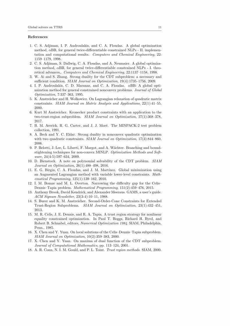
Figures 7-11 (after references) quantify the cluster effect for each solver on ourtest set by displaying for each i = 4, 5, 6, 7 (and each solver) a scatterplot of pointscorresponding to the problems solved successfully. We denote the time needed tosolve the problem at the tolerance ε = 10−i by ti and define the quotient

qi := ti+1

ti.

In addition, a reference line for qi = 1 is drawn. Note the different scales of thevertical axes.

The cluster effect is effectively suppressed if the quotient qi is close to or below1. (Values qi < 1 mean that the higher accuracy problem was solved faster than thelower accuracy one. This may be due to inaccuracies in the measured cputime, or tothe fact that a better feasible point found by a more accurate local search lead tobetter pruning in later steps.) Values of qi around 2 to 5 indicate the presence of amild cluster effect, while values of 10 or more indicate a severe cluster effect.

Figures 7-11 show that several points in the scatterplot fall below the referenceline qi = 1. It means that the time needed to solve the problem with terminationtolerance ε = 10−i−1 is lower than the time needed to solve the same instance withε = 10−i. We observe this behavior only in instances where the execution timeis significantly smaller than 1 second and therefore it is probably caused by smalldifferences in the choices of each solver during the execution.

3.4 Comparing SDP and Branch and Bound on TTRS

We looked into the question whether the difficulty of problems concerning the qualityof SDP relaxations is related to the difficulty of problems for the current generationof branch-and-bound solvers.

In Yang and Burer [46] and Anstreicher [6], all but 56 = 10+15+31 of the 212test problems were solved with more sophisticated semidefinite relaxations, using


SOC-RLT cuts and Kronecker product constraints, respectively. According to [6],the average time to solve an instance with tolerance of ε = 10−4 and n = 20 is 2seconds.

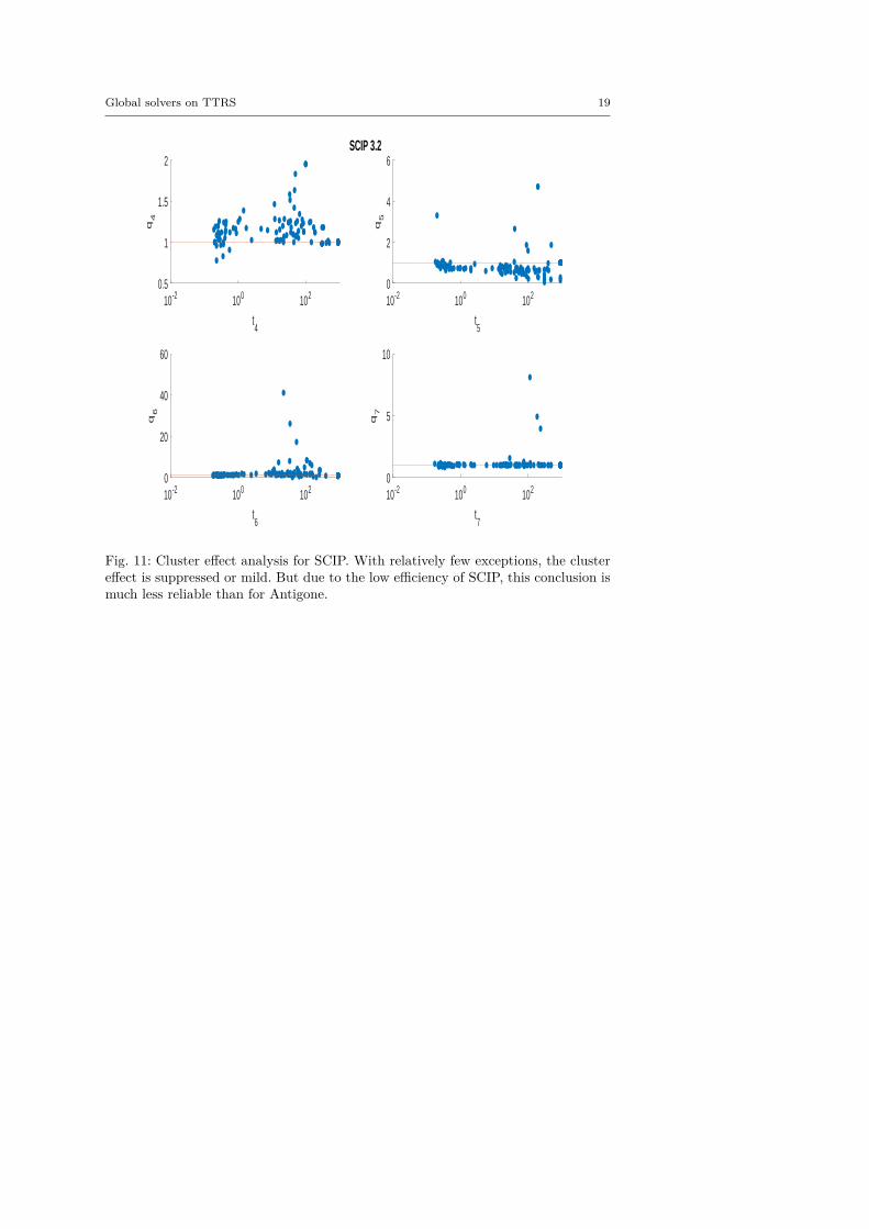
Figures 12-16 (after references) show the time needed for each branch and boundsolver to conclude the task with ε = 10−4 considering both categories of problems,easy and hard. We also display the average time described in [6] and the time limitestablished in our experiment.

One can easily see that most solvers can solve problems with n = 5 and n = 10efficiently and independent from the hardness. In particular, the average time foreach B&B solver to finish the search in the case n = 5 is lower than the averagetime required by the SDP relaxations. For n = 10 one can see that SCIP is theonly one with average time significantly greater than the SDP approach. Finally,Couenne and SCIP could not solve any instance with n = 20 within the time limitof 900 seconds, while Baron and Antigone were competitive in time with the SDPapproach. Regarding the correctness of the solution, note from Table 1 that forε = 10−4, Lindo Global is the only one with 9% of wrong claims while Baron andAntigone can find and recognize a global solution with probabilities 98% and 87%respectively. We also note that every instance not solved by Baron can be solved bySDP-relaxations.

In a branch-and-bound method, semidefinite relaxations can in principle be ap-plied at the root node, solving the problem in the ”easy” cases. In the remaining,”hard” cases, a branch-and-bound method appears to be effective but somewhatslow. Solving an SDP relaxation at selected nodes could reduce the number of nodesneeded and hence accelerate the convergence rate of the overall process. On the otherhand, solving one of the powerful SDP relaxations consumes significantly more timethan the time spent otherwise on a node. Thus while there is potential for combin-ing the approaches, it needs good judgment in how the combination is done. We arenot aware of any complete solver which combines SDP relaxations and branch-and-bound.

4 Conclusions

In conclusion, we may state that for moderate tolerances (ε ≥ 10−7), Baron is thebest and most reliable global solver among the 5 solvers tested. Antigone is secondbest if reliability matters, whereas LindoGlobal is second best if one disregards claimsof global optimality. Couenne and SCIP perform comparatively poorly and need aconsiderable strengthening to become competitive with the other solvers. All solversbecome unreliable when a high accuracy such as ε = 10−8 is requested.

Our analysis of the cluster effect indicates that Baron could benefit from an im-proved treatment of the end game in the branch-and-bound process, where the clustereffect dominates the time needed to handle the boxes very close to the solution.

We also observed that SDP relaxations and branch-and-bound have orthogonaldifficulties. This points to a possible benefit for a combination approach.


References

1. C. S. Adjiman, I. P. Androulakis, and C. A. Floudas. A global optimizationmethod, αBB, for general twice-differentiable constrained NLPs - II. implemen-tation and computational results. Computers and Chemical Engineering, 22:1159–1179, 1998.

2. C. S. Adjiman, S. Dallwig, C. A. Floudas, and A. Neumaier. A global optimiza-tion method, αBB, for general twice-differentiable constrained NLPs - I. theo-retical advances,. Computers and Chemical Engineering, 22:1137–1158, 1998.

3. W. Ai and S. Zhang. Strong duality for the CDT subproblem: a necessary andsufficient condition. SIAM Journal on Optimization, 19(4):1735–1756, 2009.

4. I. P. Androulakis, C. D. Maranas, and C. A. Floudas. αBB: A global opti-mization method for general constrained nonconvex problems. Journal of GlobalOptimization, 7:337–363, 1995.

5. K. Anstreicher and H. Wolkowicz. On Lagrangian relaxation of quadratic matrixconstraints. SIAM Journal on Matrix Analysis and Applications, 22(1):41–55,2000.

6. Kurt M Anstreicher. Kronecker product constraints with an application to thetwo-trust-region subproblem. SIAM Journal on Optimization, 27(1):368–378,2017.

7. B. M. Averick, R. G. Carter, and J. J. Moré. The MINPACK-2 test problemcollection, 1991.

8. A. Beck and Y. C. Eldar. Strong duality in nonconvex quadratic optimizationwith two quadratic constraints. SIAM Journal on Optimization, 17(3):844–860,2006.

9. P. Belotti, J. Lee, L. Liberti, F. Margot, and A. Wächter. Branching and bound-stightening techniques for non-convex MINLP. Optimization Methods and Soft-ware, 24(4-5):597–634, 2009.

10. D. Bienstock. A note on polynomial solvability of the CDT problem. SIAMJournal on Optimization, 26(1):488–498, 2016.

11. E. G. Birgin, C. A. Floudas, and J. M. Martınez. Global minimization usingan Augmented Lagrangian method with variable lower-level constraints. Math-ematical Programming, 125(1):139–162, 2010.

12. I. M. Bomze and M. L. Overton. Narrowing the difficulty gap for the Celis–Dennis–Tapia problem. Mathematical Programming, 151(2):459–476, 2015.

13. Anthony Brook, David Kendrick, and Alexander Meeraus. GAMS, a user’s guide.ACM Signum Newsletter, 23(3-4):10–11, 1988.

14. S. Burer and K. M. Anstreicher. Second-Order-Cone Constraints for ExtendedTrust-Region Subproblems. SIAM Journal on Optimization, 23(1):432–451,2013.

15. M. R. Celis, J. E. Dennis, and R. A. Tapia. A trust region strategy for nonlinearequality constrained optimization. In Paul T. Boggs, Richard H. Byrd, andRobert B. Schnabel, editors, Numerical Optimization 1984. SIAM, Philadelphia,Penn., 1985.

16. X. Chen and Y. Yuan. On local solutions of the Celis–Dennis–Tapia subproblem.SIAM Journal on Optimization, 10(2):359–383, 2000.

17. X. Chen and Y. Yuan. On maxima of dual function of the CDT subproblem.Journal of Computational Mathematics, pp. 113–124, 2001.

18. A. R. Conn, N. I. M. Gould, and P. L. Toint. Trust region methods. SIAM, 2000.


19. F. Domes, M. Fuchs, H. Schichl, and A. Neumaier. The Optimization TestEnvironment. Optimization and Engineering, 15:443–468, 2014.URL http://www.mat.univie.ac.at/˜dferi/testenv.html.

20. F. Domes and A. Neumaier. Constraint aggregation in global optimization.Mathematical Programming, 155:375–401, 2016.URL http://www.mat.univie.ac.at/˜dferi/research/Aggregate.pdf.

21. K. Du and R. B. Kearfott. The cluster problem in multivariate global optimiza-tion. Journal of Global Optimization, 5(3):253–265, 1994.URL http://interval.louisiana.edu/preprints/multcluster.pdf.

22. M. El-Alem. A global convergence theory for the Celis–Dennis–Tapia trust-region algorithm for constrained optimization. SIAM Journal on NumericalAnalysis, 28(1):266–290, 1991.

23. C. A. Floudas. Deterministic global optimization : theory, methods and applica-tions. Nonconvex optimization and its applications. Kluwer Academic Publisher,Dordrecht, Boston, London, 2000.

24. C. A. Floudas and V. Visweswaran. A global optimization algorithm (GOP) forcertain classes of nonconvex NLPs–I. theory. Computers & chemical engineering,14(12):1397–1417, 1990.

25. F. Furini, E. Traversi, P. Belotti, A. Frangioni, A. Gleixner, N. Gould, L. Liberti,A. Lodi, R. Misener, H. Mittelmann, N. Sahinidis, S. Vigerske, and A. Wiegele.QPLIB: A library of quadratic programming instances. Technical report, Febru-ary 2017. Available at Optimization Online.URL http://www.optimization-online.org/DB_HTML/2017/02/5846.html.

26. A. Goldsztejn, F. Domes, and B. Chevalier. First order rejection tests formultiple-objective optimization. Journal of Global Optimization, 58:653–672,2014.URL http://www.mat.univie.ac.at/˜dferi/research/FirstOrder.pdf.

27. G. Li. On KKT points of Celis-Dennis-Tapia subproblem. Science in ChinaSeries A, 49(5):651–659, May 2006.

28. G. Li and Y. Yuan. Compute a Celis-Dennis-Tapia step. Journal of Computa-tional Mathematics, pp. 463–478, 2005.

29. Y. Lin and L. Schrage. The global solver in the LINDO API. OptimizationMethods & Software, 24(4-5):657–668, 2009.

30. J. M. Martınez. Local minimizers of quadratic functions on Euclidean balls andspheres. SIAM Journal on Optimization, 4(1):159–176, 1994.

31. R. Misener and C. A. Floudas. Global optimization of mixed-integerquadratically-constrained quadratic programs (MIQCQP) through piecewise-linear and edge-concave relaxations. Math. Program. B, 136(1):155–182, 2012.http://www.optimization-online.org/DB_HTML/2011/11/3240.html.

32. R. Misener and C. A. Floudas. GloMIQO: Global mixed-integer quadratic opti-mizer. Journal of Global Optimization, 57(1):3–50, 2013. ISSN 0925-5001.URL http://dx.doi.org/10.1007/s10898-012-9874-7.

33. R. Misener and C. A. Floudas. Antigone: Algorithms for continuous / integerglobal optimization of nonlinear equations. Journal of Global Optimization, 59(2):503–526, 2014. ISSN 1573-2916.

34. Ruth Misener, James B Smadbeck, and Christodoulos A Floudas. Dynamicallygenerated cutting planes for mixed-integer quadratically constrained quadraticprograms and their incorporation into glomiqo 2. Optimization Methods andSoftware, 30(1):215–249, 2015.

http://www.mat.univie.ac.at/~dferi/testenv.html

http://www.mat.univie.ac.at/~dferi/research/Aggregate.pdf

http://interval.louisiana.edu/preprints/multcluster.pdf

http://www.optimization-online.org/DB_HTML/2017/02/5846.html

http://www.mat.univie.ac.at/~dferi/research/FirstOrder.pdf

http://www.optimization-online.org/DB_HTML/2011/11/3240.html

http://dx.doi.org/10.1007/s10898-012-9874-7


35. A. Neumaier. Interval methods for systems of equations, vol. 37 of Encyclopediaof Mathematics and its Applications. Cambridge Univ. Press, Cambridge, 1990.

36. A. Neumaier, O. Shcherbina, W. Huyer, and T. Vinko. A comparison of completeglobal optimization solvers. Mathematical Programming B, 103:335–356, 2005.

37. P. Nie. CDT like approaches for the system of nonlinear equations. AppliedMathematics and Computation, 172(2):892–902, 2006.

38. J. M. Peng and Y. Yuan. Optimality conditions for the minimization of aquadratic with two quadratic constraints. SIAM Journal on Optimization, 7(3):579–594, 1997.

39. A. Takeda S. Sakaue, Y. Nakatsukasa and S. Iwata. A polynomial-timealgorithm for nonconvex quadratic optimization with two quadratic constraints.in preparation, 2015.URL http://www.keisu.t.u-tokyo.ac.jp/research/techrep/data/2015/METR15-03.pdf.

40. N. V. Sahinidis. BARON 12.1.0: Global Optimization of Mixed-Integer NonlinearPrograms, User’s Manual, 2013.URL http://www.gams.com/dd/docs/solvers/baron.pdf.

41. H. Schichl, M. C. Markot, and A. Neumaier. Exclusion regions for optimizationproblems. Journal of Global Optimization, 59(2-3):569–595, 2014.

42. H. Schichl and A. Neumaier. Exclusion Regions for Systems of Equations. SIAMJournal on Numerical Analysis, 42(1):383–408, 2004.

43. S. Vigerske and A. Gleixner. SCIP: global optimization of mixed-integer non-linear programs in a branch-and-cut framework. Technical Report 16-24, ZIB,Takustr.7, 14195 Berlin, 2016.

44. V. Visweswaran and C. A. Floudas. A global optimization algorithm (GOP) forcertain classes of nonconvex NLPs–II. application of theory and test problems.Computers & chemical engineering, 14(12):1419–1434, 1990.

45. V. Visweswaran and C. A. Floudas. New properties and computational improve-ment of the GOP algorithm for problems with quadratic objective functions andconstraints. Journal of Global Optimization, 3(4):439–462, 1993.

46. B. Yang and S. Burer. A two-variable approach to the two-trust-region subprob-lem. SIAM Journal on Optimization, 26(1):661–680, 2016.

47. J. Yuan, M. Wang, W. Ai, and T. Shuai. New Results on Narrowing the DualityGap of the Extended Celis-Dennis-Tapia Problem. SIAM Journal on Optimiza-tion, 27(2):890–909, 2017.

48. Y. Yuan. On a subproblem of trust region algorithms for constrained optimiza-tion. Mathematical Programming, 47(1):53–63, 1990.

49. Y. Yuan. Recent advances in trust region algorithms. Mathematical Program-ming, 151(1):249–281, 2015.

50. A. Zhang and S. Hayashi. Celis-Dennis-Tapia based approach to quadratic frac-tional programming problems with two quadratic constraints. Numerical AlgebraControl Optimization, 1(1):83–98, 2011.

http://www.keisu.t.u-tokyo.ac.jp/research/techrep/data/2015/METR15-03.pdf

http://www.keisu.t.u-tokyo.ac.jp/research/techrep/data/2015/METR15-03.pdf

http://www.gams.com/dd/docs/solvers/baron.pdf


1 2 3 4 5 6 7 8 9 10

Time factor

0

10

20

30

40

50

60

70

80

90

100P

erc

ent of m

odels

Tol = 1e-4

Antigone 1.1Baron 16.12.7Couenne 0.5SCIP 3.2LindoGlobal 10.0

Fig. 2: Performance profile for each solver with termination tolerance 10−4.

1 2 3 4 5 6 7 8 9 10

Time factor

0

10

20

30

40

50

60

70

80

90

100

Perc

ent of m

odels

Tol = 1e-5




1 2 3 4 5 6 7 8 9 10

Time factor

0

10

20

30

40

50

60

70

80

90

100P

erc

ent of m

odels

Tol = 1e-6



1 2 3 4 5 6 7 8 9 10

Time factor

0

10

20

30

40

50

60

70

80

90

100

Perc

ent of m

odels

Tol = 1e-7




1 2 3 4 5 6 7 8 9 10

Time factor

0

10

20

30

40

50

60

70

80

90

100P

erc

ent of m

odels

Tol = 1e-8



10-2 100 102

t4

0

5

10

15

q4

Antigone 1.1

10-2 100 102

t5

0

2

4

6

q5

10-2 100 102

t6

0

2

4

6

q6

10-2 100 102

t7

0

20

40

q7

Fig. 7: Cluster effect analysis for Antigone. With relatively few exceptions, the clustereffect is suppressed or mild. This may be due to special techniques implemented onlyin Antigone for quadratic problems


10-2 100 102

t4

0

20

40q

4Baron 16.12.7

10-2 100 102

t5

0

5

10

q5

10-2 100 102

t6

0

50

100

150

q6

10-2 100 102

t7

0

20

40

q7

Fig. 8: Cluster effect analysis for Baron. There are a significant number of problemswith a severe cluster effect, except for the easily solved problems.

10-2 100 102

t4

0

1

2

3

q4

Couenne 0.5

10-2 100 102

t5

0.8

1

1.2

q5

10-2 100 102

t6

0.8

1

1.2

q6

10-2 100 102

t7

0.8

1

1.2

q7

Fig. 9: Cluster effect analysis for Couenne. In the problems solved to completion,the cluster effect is virtually absent. But this is mainly due to the fact that Couennefails to complete the search in a large proportion of cases, and this failure is due toa cluster effect not visible in the present analysis.


10-2 100 102

t4

0

1

2q

4

Lindo Global 10.0

10-2 100 102

t5

0

1

2

3

q5

10-2 100 102

t6

0

0.5

1

1.5

q6

10-2 100 102

t7

0.5

1

1.5

2

q7

Fig. 10: Cluster effect analysis for LindoGlobal. There is virtually no visible clustereffect. This may be related to heuristics that also leads to the lack of reliability ofLindoGlobal.


10-2 100 102

t4

0.5

1

1.5

2q

4SCIP 3.2

10-2 100 102

t5

0

2

4

6

q5

10-2 100 102

t6

0

20

40

60

q6

10-2 100 102

t7

0

5

10q

7

Fig. 11: Cluster effect analysis for SCIP. With relatively few exceptions, the clustereffect is suppressed or mild. But due to the low efficiency of SCIP, this conclusion ismuch less reliable than for Antigone.


5 10 15 20 25

28 out of 28 problems solved

10-5

100

105

n =

5T

ime

(s)

Easy problems with Antigone 1.1

1 2 3 4 5 6 7 8 9 10


10-5

100

105

Tim

e(s

)

Hard problems with Antigone 1.1

5 10 15 20 25 30 35 40 45 50 55


10-5

100

105

n =

10

Tim

e(s

)

2 4 6 8 10 12 14


10-5

100

105

Tim

e(s

)

10 20 30 40 50 60 70


100

102

104

n =

20

Tim

e(s

)

5 10 15 20 25 30


100

102

104

Tim

e(s

)

Execution time(s) Time Limit(900s) Average SDP(2s)

Fig. 12: Sorted execution time for Antigone to solve the 212 instances classified aseasy and hard according to the definition in Section 2.3 with termination tolerance ofε = 10−4. The dashed lines displays the average time of the SDP relaxation approachreported in [6].


5 10 15 20 25


10-5

100

105

n =

5T

ime

(s)

Easy problems with Baron 16.12.7

1 2 3 4 5 6 7 8 9 10


10-5

100

105

Tim

e(s

)

Hard problems with Baron 16.12.7

5 10 15 20 25 30 35 40 45 50 55


10-5

100

105

n =

10

Tim

e(s

)

2 4 6 8 10 12 14


10-5

100

105

Tim

e(s

)

10 20 30 40 50 60 70


100

102

104

n =

20

Tim

e(s

)

5 10 15 20 25 30


100

102

104

Tim

e(s

)


Fig. 13: Sorted execution time for Baron to solve the 212 instances classified aseasy and hard according to the definition in Section 2.3 with termination toleranceof ε = 10−4. The dashed lines displays the average time of the SDP relaxationapproach reported in [6].


5 10 15 20 25


10-5

100

105

n =

5T

ime

(s)

Easy problems with Lindo Global 10.0

1 2 3 4 5 6 7 8 9 10


10-5

100

105

Tim

e(s

)

Hard problems with Lindo Global 10.0

5 10 15 20 25 30 35 40 45 50 55


10-5

100

105

n =

10

Tim

e(s

)

2 4 6 8 10 12 14


10-5

100

105

Tim

e(s

)

10 20 30 40 50 60 70


10-5

100

105

n =

20

Tim

e(s

)

5 10 15 20 25 30


10-5

100

105

Tim

e(s

)


Fig. 14: Sorted execution time for Lindo Global to solve the 212 instances classified aseasy and hard according to the definition in Section 2.3 with termination tolerance ofε = 10−4. The dashed lines displays the average time of the SDP relaxation approachreported in [6].


5 10 15 20 25


10-5

100

105

n =

5T

ime

(s)

Easy problems with Couenne 0.5

1 2 3 4 5 6 7 8 9 10


10-5

100

105

Tim

e(s

)

Hard problems with Couenne 0.5

5 10 15 20 25 30 35 40 45 50 55


10-5

100

105

n =

10

Tim

e(s

)

2 4 6 8 10 12 14


100

102

104

Tim

e(s

)

10 20 30 40 50 60 70


100

102

104

n =

20

Tim

e(s

)

5 10 15 20 25 30


100

102

104

Tim

e(s

)


Fig. 15: Sorted execution time for Couenne to solve the 212 instances classified aseasy and hard according to the definition in Section 2.3 with termination tolerance ofε = 10−4. The dashed lines displays the average time of the SDP relaxation approachreported in [6].


5 10 15 20 25


10-5

100

105

n =

5T

ime

(s)

Easy problems with SCIP 3.2

1 2 3 4 5 6 7 8 9 10


10-5

100

105

Tim

e(s

)

Hard problems with SCIP 3.2

5 10 15 20 25 30 35 40 45 50 55


100

102

104

n =

10

Tim

e(s

)

2 4 6 8 10 12 14


100

102

104

Tim

e(s

)

10 20 30 40 50 60 70


100

102

104

n =

20

Tim

e(s

)

5 10 15 20 25 30


100

102

104

Tim

e(s

)


Fig. 16: Sorted execution time for SCIP to solve the 212 instances classified as easyand hard according to the definition in Section 2.3 with termination tolerance ofε = 10−4. The dashed lines displays the average time of the SDP relaxation approachreported in [6].

Documents

A computational study of global optimization solvers on ... · 2 Tiago Montanher et al. 1 Introduction Quadratically constrained quadratic programming (QCQP) is the task of ﬁnding