A COMPUTATIONAL FLUID DYNAMICS ANALYSIS OF SIMPLE MATHEMATICALLY DESIGNED HULL FORMS FOR GLIDER

APPLICATIONS

by

Perri Quattrociocchi

Bachelor of Science Oceanography

Florida Institute of Technology 2010

A thesis submitted to the Department of Marine and Environmental Sciences at Florida Institute of Technology in partial fulfillment of the requirements for the degree of

Master of Science In

Ocean Engineering

Melbourne, FL December, 2012

We the undersigned committee hereby approve the attached thesis

A Computational Fluid Dynamics Analysis of Simple Mathematically Designed Hull Forms for Glider Applications

by Perri Quattrociocchi

________________________________ Stephen Wood, Ph.D., P.E. Professor and Head, Ocean Engineering Major Advisor, Committee Chair

________________________________ Ronnal Reichard, Ph.D. Professor, Ocean Engineering Director of Laboratories Committee Member

________________________________ Luis Otero, Ph.D. Professor, Engineering Systems Committee Member

iii

ABSTRACT

A Computational Fluid Dynamics Analysis of Simple Mathematically Designed

Hull Forms for Glider Applications

by

Perri Quattrociocchi

Committee Chair: Stephen Wood, Ph.D., P.E.

Gliders are long-range, long-term vehicles that gather imperative information for the

commercial, scientific, defense and educational industries. They are cheaper than the

larger, powered Autonomous Underwater Vehicles (AUVs) and can perform many of the

same types of operations, including: inspecting pipelines; surveying cables; locating areas

of interest or specific targets; inspecting underwater contacts; ocean sampling, and

environmental monitoring. Currently, commercial gliders and AUVs are expensive to

purchase and are limited to the manufacturer’s payload due to the vehicle hull

dimensions and proprietary designs. The production of a simple mathematically designed

hull, that can be scalable and easy to build at a low cost, is needed to improve and expand

on the versatility of the gliders. In this study, four glider hulls were created from simple

mathematical equations, resulting in an Elliptical-Parabolic Hull, an Elliptical-Cubic Hull, a

Parabolic-Parabolic Hull and a Parabolic-Cubic Hull. SolidWorks Flow Simulation was used

for the Computational Fluid Dynamics (CFD) analysis at the speeds of 0.1 knot, 0.5 knot

and 1 knot, to find the optimum hydrodynamic efficiency out of the four glider hull

designs.

iv

It is hypothesized that the following parameters affect the movement of the vehicle:

Pressure on the hull exerts additional force, dependent on geometry, which the vehicle

must account for in order to move through the water. The velocity along the hull is a

potential indicator of the overall percentage of drag created by the hull’s geometry. The

turbulent viscosity can create drag along the middle section of the hull. The friction

coefficient is a measure of the boundary layer friction occurring on the hull. The drag

force and the corresponding drag coefficients show how much drag is created and how

much that drag affects the vehicle in relation to other forces. The Reynolds Numbers for

each hull at each speed determine whether the movement around the hull is laminar or

turbulent. The goals of this study were aimed at comparing the hulls in terms of the drag

force, corresponding drag coefficient and the resulting Reynolds numbers for each model.

The analysis showed the following: The pressure was found to be of no real significance

due to the low speeds at which the hulls were tested. The velocity results indicated that

the Parabolic Bows may create more efficient streamlining (lower velocity maximums)

through the water, therefore, the least drag across the entirety of the hulls. From the

turbulent viscosity, the Parabolic Tail design created the lowest maximums, yet the effect

on drag was not verifiable. The friction coefficient analysis suggests that the Elliptical-

Parabolic Hull is the optimum choice with a value of 0.02183, while the drag coefficient

suggests that the Elliptical-Cubic Hull is the best with a value of 0.01065. The Reynolds

number was lowest for the Parabolic-Parabolic Hull. Overall, the Elliptical-Parabolic Hull

v

rated highly in each viable analysis. The results were too close in each parameter in order

to definitively determine which vehicle was the most hydrodynamically efficient. Despite

lacking in customizability, SolidWorks was deemed a viable tool for CFD. This study is an

essential step to providing a simple mathematically designed glider hull for various

scientific applications. Additional work will be needed to further validate the findings.

vi

Table of Contents

List of Figures…………………………………………………………………………………………………………………viii

List of Tables……………………………………………………………………………………………………………………..x

List of Abbreviations…………………………………………………………………………………………………………xi

List of Symbols…………………………………………………………………………………………………………………xii

Acknowledgements………………………………………………………………………………………………………..xiv

1. Introduction………………………………………………………………………………………………………………….1

1.1 Operation………………………………………………………………………………………………………2

1.2 Experimental Parameters……………………………………………………………………………..3

2. Background…………………………………………………………………………………………………………………..6

3. Hull Forms……………………………….………………………………………………………………………………….20

3.1 Hull Equations………………………………………………………………………………………………21

3.2 Models…..…………………………………………………………………………………………………….22

4. Computational Fluid Dynamics Analysis……………………………………………………………………..24

4.1 Methods………………………………………………………………………………………………………25

4.1.1 Set Conditions………………………………………………………………………………25

4.1.2 Goals…………………………………………………………………………………………….26

5. Results………………………………………………………………………………………………………………………..29

5.1 Pressure……………………………………………………………………………………………………….29

5.2 Velocity………………………………………………………………………………………………………..32

vii

5.3 Friction Coefficient……………………………………………………………………………………..35

5.4 Turbulent Viscosity……………………………………………………………………………………..37

5.5 Drag Force and Drag Coefficient………………………………………………………………….40

5.6 Reynolds Numbers………………………………………………………………………………………43

6. Discussion……………………………………………………………………………………………………………………44

6.1Pressure………………………………………………………………………………………………………..44

6.2 Velocity………………………………………………………………………………………………………..45

6.3 Friction Coefficient……………………………………………………………………………………….46

6.4 Turbulent Viscosity……………………………………………………………………………………….46

6.5 Drag Force, Drag Coefficient and Reynolds Number……………………………………47

7. Conclusions…………………………………………………………………………………………………………………49

8. Future Work……………………………………………………………………………………………………………….51

9. References…………………………………………………………………………………………………………………53

10. Appendix………………………………………………………………………………………………………………….56

viii

List of Figures

Figure 1: Teledyne-Webb Slocum Electric Glider dive pattern…………………………………………3

Figure 2: Slocum by Teledyne-Webb………………………………………………………………………………..6

Figure 3: Spray Glider by Bluefin Robotics………………………………………………………………………..7

Figure 4: Seaglider, top and Deepglider, bottom, by APL…………………………………………………7

Figure 5: ALEX Glider…………………………………………………………………………………………………………8

Figure 6: NTU Glider, Version 2A…………………………………………………………………………………….10

Figure 7: USM Glider……………………………………………………………………………………………………….11

Figure 8: SeaDiver II………………………………………………………………………………………………………..12

Figure 9: XRay Flying Wing Glider……………………………………………………………………………………12

Figure 10: Pressure Distributions on the hull of PICASSO………………………………………………15

Figure 11: Rounded Bow sections for PICASSO………………………………………………………………16

Figure 12: Extended Tail sections for PICASSO……………………………………………………………….16

Figure 13: Laminar Flow Body example…………………………………………………………………………..17

Figure 14: Autosub by the National Marine Facilities at USL……………………………………………17

Figure 15: Autosub engineering trials for the ancillary component of drag……………………..18

Figure 16: Elliptical-Parabolic Hull..................................................................................23

Figure 17: Elliptical-Cubic Hull ......................................................................................23

Figure 18: Parabolic-Parabolic Hull................................................................................24

Figure 19: Parabolic-Cubic Hull .....................................................................................24

ix

Figure 20: Pressure on the Parabolic-Parabolic Hull at 1 knot (0.514 m/s)………………………30

Figure 21: Pressure on the Parabolic-Cubic Hull at 1 knot (0.514 m/s)…………………………….30

Figure 22: Pressure on the Elliptical-Parabolic Hull at 1 knot (0.514 m/s)………………………..31

Figure 23: Pressure on the Elliptical-Cubic Hull at 1 knot (0.514 m/s)..............................31

Figure 24: Velocity around the Parabolic-Parabolic Hull at 1 knot (0.514 m/s)………………..33

Figure 25: Velocity around the Parabolic-Cubic Hull at 1 knot (0.514 m/s) ……………………..33

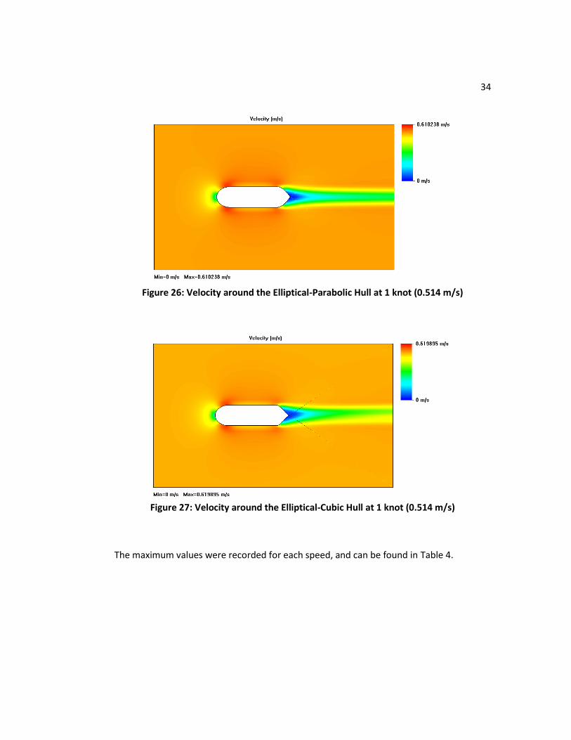
Figure 26: Velocity around the Elliptical-Parabolic Hull at 1 knot (0.514 m/s)………………….34

Figure 27: Velocity around the Elliptical-Cubic Hull at 1 knot (0.514 m/s..........................34

Figure 28: Friction Coefficient on the Parabolic-Parabolic Hull at 1 knot (0.514 m/s)........35

Figure 29: Friction Coefficient on the Parabolic-Cubic Hull at 1 knot (0.514 m/s)..............36

Figure 30: Friction Coefficient on the Elliptical-Parabolic Hull at 1 knot (0.514 m/s).........36

Figure 31: Friction Coefficient on the Elliptical-Cubic Hull at 1 knot (0.514 m/s)...............37

Figure 32: Turbulent Viscosity along the Parabolic-Parabolic Hull at 1 knot (0.514 m/s)...38

Figure 33: Turbulent Viscosity along the Parabolic-Cubic Hull at 1 knot (0.514 m/s)……….38

Figure 34: Turbulent Viscosity along the Elliptical-Parabolic Hull at 1 knot (0.514 m/s).....39

Figure 35: Turbulent Viscosity along the Elliptical-Cubic Hull at 1 knot (0.514 m/s)...........39

Figure 36: Drag Force and Drag Coefficients for each Hull Type.........................................41

Figure 37: Reynolds Number for each hull type at each speed……………………………...........43

Figure 38: Pulley system for Pull Test ..…………………………………………………………..................52

x

List of Tables

Table 1: Principal Characteristics of ALEX………………………………………………………………………....9

Table 2: Model Dimensions…………………………………………………………………………………….........23

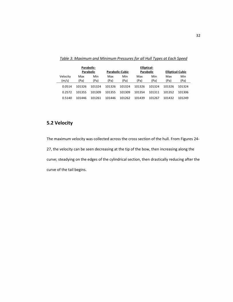
Table 3: Maximum and Minimum Pressures for all Hull Types at Each Speed………………..32

Table 4: Maximum Velocity around all Hull Types at Each Speed…………………………………...35

Table 5: Average Friction Coefficients on all Hull Types at Each Speed……………………………37

Table 6: Maximum and Minimum Turbulent Viscosity along all Hull Types at

Each Speed.............................................................................................................40

Table 7: Drag Force and Drag Coefficient Averages for each Hull Type……………………………41

Table 8: Statistical Significance of Drag Force between each of the Hull Types……………….42

xi

List of Abbreviations

APL: Applied Physics Laboratory

AUV: Autonomous Underwater Vehicle

CFD: Computational Fluid Dynamics

GPS: Global Positioning System

ITTC-57: International Towing Tank Conference (1957)

NACA: National Advisory Committee for Aeronautics

NTU: National Taiwan University

PICASSO: Plankton Investigatory Collaborating Autonomous Survey System Operation

ROV: Remotely Operated Vehicle

USM: Universiti Sains Malaysia

xii

List of Symbols

Aw: Wetted surface area

B: Length of bow section

CD: Drag coefficient

CF: Friction resistance coefficient

d: Vessel diameter

FX, FD: Drag force

l: Vessel length

μ: Dynamic viscosity

n: Degrees of freedom

ρ: Density

R: Maximum vehicle radius

ReL: Reynolds number as a function of length

S: Projected Area

: Standard deviation of the data sets

T: Statistical t-value

T: Length of tail section

V, U: Velocity

X: Length

: Mean of the first model

xiii

: Mean of the second model

Z: Radius

xiv

Acknowledgements

This thesis could not have been completed without the help of a long list of supporters

and helpers.

- To Anthony Jones who not only helped with the creation of this thesis, but was a

constant source of information and support along the way.

- To Dr. Stephen Wood who pushed me to do my best, and constantly reminded me that

working on this study came before anything else.

- To my committee members, Dr. Luis Otero and Dr. Ronnal Reichard who took on this

study despite the time restrictions and difficulties of completing a meaningful thesis in

just a couple months.

- To my parents, Bethany and Michael Quattrociocchi, Kenneth Castoro, Phillip Meyer,

and Anthony Jones for taking the time to help with the editing process.

- To all of the students in the Ocean Engineering Lab who contributed words of wisdom

and support.

Thank you.

1

1. Introduction

Over the last couple decades, the need for underwater vehicles has grown dramatically.

These vehicles have critical roles in the oil industry for inspecting pipelines, surveying

cables, and locating areas of interest; in the defense/military industry for surveying varied

environments, locating targets and inspecting underwater contacts; and in the scientific

research field for ocean sampling and environmental monitoring [17]. Starting with

Remotely Operated Vehicles (ROVs) and then Autonomous Underwater Vehicles (AUVs),

the evolution of underwater vehicles has come a long way. Glider type vehicles are in the

infancy of development since their initial introduction in the 1980s with Henry Stommel

[10]. The vehicles can cover greater distances, for longer periods of time with less human

interaction, and with a lower cost than conventional AUVs [15].

With their longer range and lower cost, gliders are an exceptional addition to the

scientific community. Gliders depend on changes in net buoyancy for propulsion, thus

optimizing the hydrodynamics of the hull is a high priority. If the drag becomes too great,

the speed as well as the glider’s ability to propagate through the water at a consistent

rate suffers [25]. Consequently, the hull design is only useful if the hydrodynamics provide

minimal drag. Experimental testing to provide hydrodynamic analysis, such as in tow

tanks and circulating water channels is very time consuming and costly; while

computational fluid dynamics (CFD) analyses are less time consuming and less costly, but

2

still provide reliable results [17] provided that the bodies are simple and streamlined as in

the hulls of this study.

1.1 Operation

As the gliders adjust their buoyancy to move up and down, the lift-drag on the wings, hull

and tailfins generate the horizontal movement through the water; creating a saw-toothed

trajectory [27]. The speeds during surveying are typically very low (starting around 0.1

knots or 0.0514 m/s) and generally do not exceed 1 knot (0.514 m/s), depending on the

design. The current glider flight durations range from hours underwater to days. Figure 1

shows Teledyne-Webb’s Slocum Electric Glider, which requires surfacing at least every 24

hours and can only dive to depths of 200 m. The maximum depths of gliders range as well;

currently the average diving depth is around 1000 m.

3

Figure 1: Teledyne-Webb Slocum Electric Glider dive pattern [15]

1.2 Experimental Parameters

Hull geometry is a large determinant of how efficiently the vehicle moves through the

water. The drag force and the resulting drag coefficient are two important parameters

that can affect the movement of the vehicle. The goals of the project were aimed in

comparing the hulls in terms of the drag force, corresponding drag coefficient and the

resulting Reynolds numbers for each model. However, there are other parameters to

determine as well. These parameters are:

4

Pressure: The pressure on the hull contributes to the force that is obstructing the

vehicle. The greater the pressure, the more power the vehicle needs to push

through the water. Minimizing the pressure at the bow through the hull geometry

can reduce some of the force.

Velocity: Hull geometry’s impact on velocity is very important for the overall

movement of the vehicle. When the wings of the glider are attached, the increase

in velocity along the edges of the hull may allow for greater lift, dependent on

design, and therefore more efficient movement through the water. A study by

D.F. Myring concluded that the bodies which produce higher velocities tend to

exhibit higher percentages of form drag [13]. Thus, the hull with the lowest velocity

maxima may be more hydrodynamically efficient.

Turbulent Viscosity: The turbulent viscosity can influence drag if the bow

produces turbulence against the sides of the cylindrical middle or along the tail.

This parameter can also show the streamlining of the hull by the wake that it

produces. Although this study deals with slower speeds (less than 0.514 m/s),

there is a possibility that turbulence has a slight effect on the drag along the back

end of the hull.

5

Friction Coefficient: The friction coefficient is a measure of the boundary layer

friction between the fluid and the hull. This value is very important to the overall

drag since it isolates the areas of higher friction. Simply put, the greater the

friction, the greater the drag. In the case of this study, the friction coefficient

results were expected to decrease with speed and to be on the same order as the

drag coefficient, and therefore of considerable importance.

In order to analyze these various parameters, a CFD analysis of the glider hull forms at

equal volumes is needed. This study used SolidWorks Flow Simulation in order to find the

values for each parameter. The general hull forms were based on simple cubic, elliptical

and parabolic equations for the bow and tail. This resulted in the modeling of a Parabolic-

Parabolic Hull, a Parabolic-Cubic Hull, an Elliptical-Parabolic Hull and an Elliptical-Cubic

Hull. The results of this study were meant to provide a very simple base of equations for

building a hydrodynamically efficient glider hull for various scientific applications.

6

2. Background

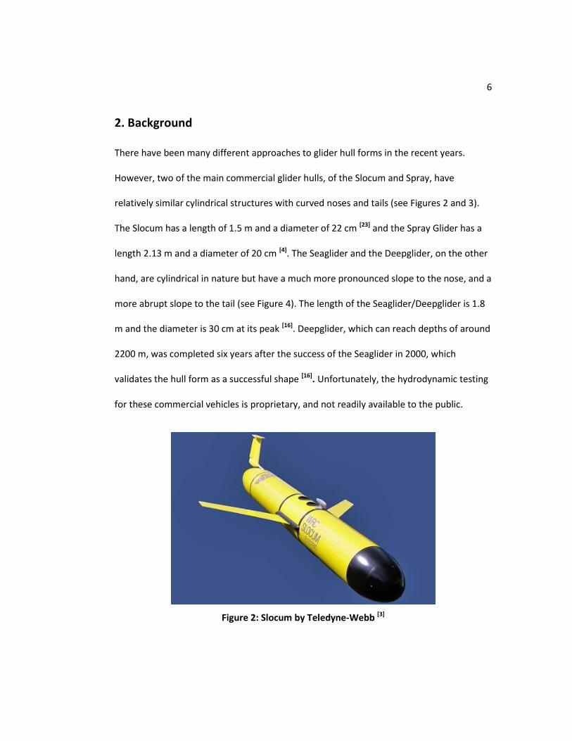
There have been many different approaches to glider hull forms in the recent years.

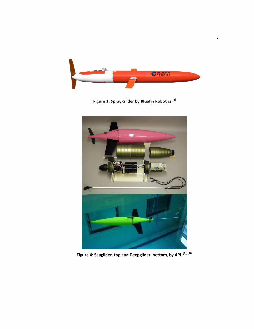
However, two of the main commercial glider hulls, of the Slocum and Spray, have

relatively similar cylindrical structures with curved noses and tails (see Figures 2 and 3).

The Slocum has a length of 1.5 m and a diameter of 22 cm [23] and the Spray Glider has a

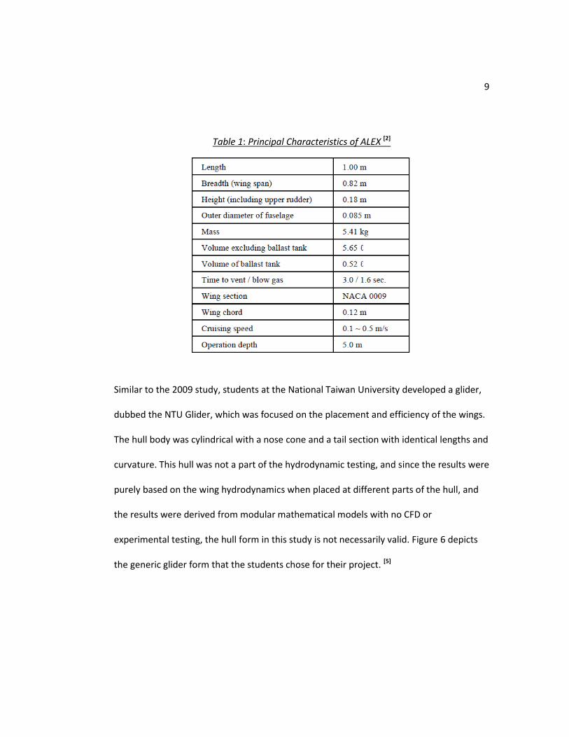
length 2.13 m and a diameter of 20 cm [4]. The Seaglider and the Deepglider, on the other

hand, are cylindrical in nature but have a much more pronounced slope to the nose, and a

more abrupt slope to the tail (see Figure 4). The length of the Seaglider/Deepglider is 1.8

m and the diameter is 30 cm at its peak [16]. Deepglider, which can reach depths of around

2200 m, was completed six years after the success of the Seaglider in 2000, which

validates the hull form as a successful shape [16]. Unfortunately, the hydrodynamic testing

for these commercial vehicles is proprietary, and not readily available to the public.

Figure 2: Slocum by Teledyne-Webb [3]

7

Figure 3: Spray Glider by Bluefin Robotics [4]

Figure 4: Seaglider, top and Deepglider, bottom, by APL [1], [16]

8

A study in 2009 created the ALEX Glider, which used a nose with a NACA0050 shape (see

Figure 5) that the author dubbed “suitable for modelling [sic] and estimating the

hydrodynamic forces,” but did not provide any supporting research or data for the

specific hull form [2].The hull dimensions of the glider can be seen in Table 1. The study

demonstrates the use of CFD as a reliable tool for estimating hydrodynamic forces on

glider forms, including the lift and drag forces acting on all surfaces, in varied conditions

for all angles of incidence. The authors used a commercial program by Software Cradle

Co., Ltd. called SC/Tetra, which uses three dimensional CFD similar to that of SolidWorks

Flow Simulation. The results of this study were based around the performance of

independently controllable wings; however, since the hull form has a large part to do with

the success of the glider overall, the choice of curvature for the nose cone can be

validated by the positive results of the study.[2]

Figure 5: ALEX Glider [2]

9

Table 1: Principal Characteristics of ALEX [2]

Similar to the 2009 study, students at the National Taiwan University developed a glider,

dubbed the NTU Glider, which was focused on the placement and efficiency of the wings.

The hull body was cylindrical with a nose cone and a tail section with identical lengths and

curvature. This hull was not a part of the hydrodynamic testing, and since the results were

purely based on the wing hydrodynamics when placed at different parts of the hull, and

the results were derived from modular mathematical models with no CFD or

experimental testing, the hull form in this study is not necessarily valid. Figure 6 depicts

the generic glider form that the students chose for their project. [5]

10

Figure 6: NTU Glider, Version 2A [5]

The Universiti Sains Malaysia (USM) created an underwater glider in 2011 based on the

“Slender-Body Theory” [10]. The Slender-body Theory states that if the diameter is much

less than the length of a straight object, then one can think of the body as a longitudinal

stack of thin sections with an easily computed added mass [24]. This “slender-body” glider

hull had a length of 1.4 m and a diameter of 17 cm (see Figure 7). The authors of this

study used MATLAB to define the drag forces upon the vehicle instead of a CFD program

or experimental testing. Although, mathematically correct, this does not necessarily show

the drag forces on each surface of the vehicle, and it treats the vehicle as a “slender-

body” which creates assumptions to the mass and more finite details. [10]

11

Figure 7: USM Glider [10]

The SeaDiver/SeaDiver II Glider and the XRay Flying Wing Glider are two examples of

large-body gliders. These models are generally made for long-term, long-range

deployments. The SeaDiver Glider was originally proposed and built by the University of

Toulon, France, and was tested with help from the Naval Post Graduate School. The

SeaDiver hull was shaped after an airfoil, while the XRay Glider* is shaped more like a

fighter jet plane (See Figures 8 and 9). Unfortunately, the SeaDiver was not proven to be a

valid glider and was found to need further development in both the software systems as

well as the overall hull construction. [8]

* The XRay Flying Wing Glider turned out to be a successful tool for the Office of Naval Research, but no

hydrodynamic analyses were found in the literature.

12

Figure 8: SeaDiver II [8]

Figure 9: XRay Flying Wing Glider [1]

13

In 2007, authors Phillips, Furlong and Turnock provided a study on hull forms for

AUVs/gliders using three distinct nose cones: circular, 2-1 ellipsoid and 3-1 ellipsoid.

These AUV forms were modeled based on the following equation in order to estimate the

form factor for a streamlined body as a function of vessel length (l) and diameter (d):

(I + k) = I + 1.5(d/I)3/2 + 7(d/I)3

Using this equation allowed the authors to get an initial estimate of the powering

requirements. The forms were created in ANSYS ICEM CFD and the drag of the hulls was

modeled through the Reynolds Averaged Navier-Stokes Equation and analyzed by

Reynolds Number created by each hull. The study was then expanded to include

previously built AUVs, which were analyzed for drag along the hull and compared to

existing experimental results. The results showed that CFD is a valid form of

hydrodynamic testing for all concept hull forms when compared to existing experimental

data. Further, it was found that CFD analysis can also be used “to determine straight line

resistance of bare and appended hull forms; allow rapid comparison of the resistance of

different hull forms at the initial design stage through the use of highly parameterised

geometric models; to complement model test experiments, to gain a clearer

understanding of the origins of measured drag and to help understand the effect of test

conditions on the open water performance of these vehicles; and to provide detailed

14

information about the mean flow pattern around the hull which would not normally be

determined from standard towing tank experiments.” [17]

A study in 2010, of PICASSO (Plankton Investigatory Collaborating Autonomous Survey

System Operation), an AUV developed in Japan for the study of deep sea plankton, was

determined to find a way to improve the hydrodynamic efficiency of the vehicle. This

study looked at the water resistance, or the effects of pressure, upon the hull of the

vehicle. Using FLUENT, the flow field was generated around PICASSO. As seen in Figure

10, there was a large amount of pressure on the front of the bow due to the flatness of

the geometry.

15

Figure 10: Pressure Distributions on the hull of PICASSO [9]

In order to see the effects of the pressure, the drag coefficient was calculated through the

following equation:

Where the projected area used, S, was defined as the breadth of the fuselage times the

depth of the vehicle, CD is the drag coefficient, FX is the drag force, ρ is density, and V is

16

the velocity. In order to reduce the drag coefficient and the effects of pressure, new bow

sections (Figure 11), and tail sections (Figure 12), were proposed by the authors. [9]

Figure 11: Rounded Bow sections for PICASSO. [9]

Figure 12: Extended Tail sections for PICASSO. [9]

The results of changing the fore and aft sections were positive. The best configuration

was found to be the most rounded bow paired with the most extended tail. This study

found many discrepancies between the theoretical and experimental values [9]. The CFD

simulation used appeared adequate; however, due to the discrepancies found, the

equations used in the software needed to be either more accurate or more targeted

towards the preferred outputs.

17

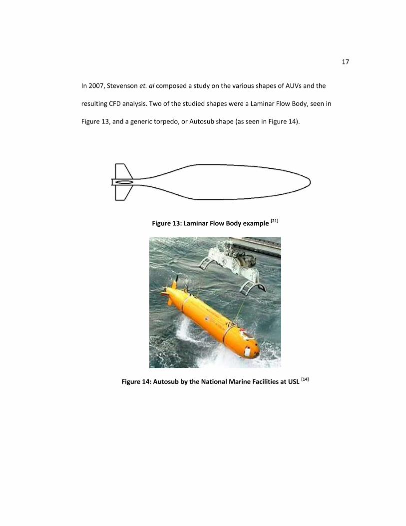
In 2007, Stevenson et. al composed a study on the various shapes of AUVs and the

resulting CFD analysis. Two of the studied shapes were a Laminar Flow Body, seen in

Figure 13, and a generic torpedo, or Autosub shape (as seen in Figure 14).

Figure 13: Laminar Flow Body example [21]

Figure 14: Autosub by the National Marine Facilities at USL [14]

18

The Autosub shape is very similar to the hulls in this study. After the engineering trials of

the Autosub, it was found that the body creates almost 75% of drag on the vehicle, as

seen in Figure 15.

Figure 15: Autosub engineering trials for the ancillary component of drag [21]

After analyzing the drag coefficients in CFD software, the Laminar Flow Body created a

drag coefficient of 0.0109, while the experimental values at sea showed a drag coefficient

of 0.013-0.015. The Autosub, however, had a CFD analysis result in a drag coefficient of

0.029, not including the external appendages (fins, tail, GPS, etc.). The authors believed

19

that the CFD values were slightly lower than the experimental values would and should be

due to antennae, seams, bolts, etc. [21]

The study also took the 4-digit NACA airfoil shapes into consideration. NACA shapes were

developed to standardize the design of aircraft wings. The chosen shapes included the

NACA0010, NACA0020, NACA0033, and NACA0050. It was found that the 4-digit NACA

shapes with a length to diameter ratios between 3 and 4 had resulting drag coefficients of

approximately 0.025 and 0.0195, respectively. The drag coefficients of the forms which

had length to diameter ratios greater than 3 did not differ in value more than around

0.007. [21]

20

3. Hull Forms

This study tested the use of varied bow and tail sections on hull forms for hydrodynamic

efficiency. The glider hull designs were created with simple mathematically designed

forms including: an Elliptical Bow with a Parabolic Tail; an Elliptical Bow with Cubic Tail; a

Parabolic Bow with Parabolic Tail; and a Parabolic Bow with Cubic Tail. Since these hulls

should produce the same percentage of drag force at any size, the results of each model

allow for the hulls to be used in a wide range of applications for various payloads.

The main limitation of the glider hulls of the Seaglider and of the designs based on NACA

airfoils is space for payloads. The hulls are wide only at the center of the vehicle and have

very narrow nose and tail sections. The approach in this study allows for the use of varied

payloads by providing a cylindrical middle section that can be increased as long as the

curvature of the nose and tail are subsequently increased. The Slocum and Spray are

based on similar designs to this study; however, their designs are proprietary and not

readily available to the public. Additionally, the Slocum and Spray are only available in

one size. They only allow specific payloads to be used, which can prevent the user from

implementing a specific payload or payload addition; often allowing the parent company

to set high prices for customization and/or upgrades to the payload.

The literature found on the hydrodynamics of gliders tended to focus on the wing designs

instead of the hull design. This is could create problems considering that the movement of

21

gliders is dependent on changes in the net buoyancy and the influence of drag, which are

mainly hull related. There is not much literature available for complete hull designs that

are both scalable and fit a large number of applications. This study aimed at trying to

provide this information.

3.1 Hull Equations

This study created four equal volume glider hulls in SolidWorks:

1. Elliptical Bow with Parabolic Tail

2. Elliptical Bow with Cubic Tail

3. Parabolic Bow with Parabolic Tail

4. Parabolic Bow with Cubic Tail

The glider hulls were modeled by using the following formulas mathematically derived by

Anthony Jones [11]:

Elliptical Bow: Parabolic Bow:

√ ( )

22

Middle Body:

z=R

Parabolic Tail: Cubic Tail:

( )

( )

Where Z=radius, X=length, B=length of bow section, T=length of tail section, and

R=maximum vehicle radius. The constants included R=0.15 m, T= 0.2 m and B= 0.2 m.

3.2 Models

The cylindrical section of each hull was determined by the volume desired, keeping the

vehicle’s length at a minimum of 1 m, and diameter at 0.3 m. The bow and tail sections

were kept at lengths of 0.2 m for all models. These dimensions are based off of the

average payload need for the three commercial gliders: Spray, Slocum and Seaglider, as

well as the results of the Stevenson study, where it was found that as long as the length

to diameter ratio is between 3 and 4, the effect on the drag coefficient should be minimal

[21]. The volume for the vehicles was a constant 0.06 m3. Table 2 shows the final

measurements of each model.

23

Table 2: Model Dimensions

Model Diameter Length

Elliptical-Parabolic 0.300 m 1.060 m Elliptical-Cubic 0.300 m 1.093 m Parabolic-Parabolic 0.300 m 1.000 m Parabolic-Cubic 0.300 m 1.033 m

Below, Figures 16-19 show each of the models as screen captures from SolidWorks.

Figure 16: Elliptical-Parabolic Hull

Figure 17: Elliptical-Cubic Hull

24

Figure 18: Parabolic-Parabolic Hull

Figure 19: Parabolic-Cubic Hull

4. Computational Fluid Dynamics Analysis

SolidWorks Flow Simulation is not a fully customizable software in terms of mathematical

analysis for CFD applications. The software uses its own equations to deal with friction,

drag, viscosity, etc. It allows goal equations to be made, but does not allow changes to the

default equations. This makes the software easier to use in terms of basic analyses, but

more difficult when dealing with the finer aspects of CFD. An example of this is computing

the coefficient of drag. The software uses an equation based goal to determine the

25

coefficient. However, it did not seem able to fully compute this number for the needs of

this study. The software may have ways around this issue, but they were not found

throughout the duration of this project. It was a slight problem in the case of the glider

hulls, but adjustments needed to be made accordingly. Instead of having the software

compute the maximum, minimum and average coefficient of drag, it was used, instead, to

compute the drag force – from which the drag coefficient could then be calculated by

hand. Overall, this ended up as a benefit to the project. This way, the wetted drag

coefficient, the volumetric drag coefficient, and the relative drag coefficient could be

computed for each vehicle at each speed as needed. For the purposes of this study, the

wetted drag coefficient was used because it deals with a fully submerged vehicle. The

goals of the project, as well as the equations used are outlined in §4.1.2, aim in comparing

the hulls in terms of the drag force, corresponding drag coefficient and the resulting

Reynolds numbers for each model.

4.1 Methods

4.1.1 Set Conditions

The fluid conditions were based on the basic water parameters set in SolidWorks. These

were based off of standard temperature and pressure; specifically, a temperature of

26

293.2 K, a pressure of 101325 Pa and a resulting density of 1000 kg/m3. These values were

used in the Reynolds number and coefficient of friction equations as needed. The

software allowed the fluid to be laminar or turbulent, dependent on need, with the

turbulence set at the default value (given by SolidWorks) of 1% intensity and a turbulence

length of 0.002999999 m. The vehicles were modeled in 6061-T6 Aluminum Alloy. This

was decided upon for both aesthetics and for the commonality of the material’s use in

submerged vehicles. Additional roughness was not accounted for due to the fact that the

actual roughness will depend on the machining and coating of the vehicle after

production. The roughness would have changed the resulting values to the same degree.

The simulation was run looking only at external flow and excluded internal space (there

was no internal space to analyze, however, for consistency, this option was always

chosen). The mesh resolution was increased to level 4, allowing the minimum number of

iterations per run to be 96. For consistency, the grid size used for simulation was the

software’s default dimensions of -0.9 m to 2.56 m in the X plane, and -1.05 m to 1.05 m in

both the Y and Z planes.

4.1.2 Goals

The goals focused on five main parameters. These parameters were the pressure on the

hull, the change of velocity across the hull, the friction coefficient, the turbulent viscosity

27

and the drag force. The pressure, velocity and turbulent viscosity were all measured in the

flow simulation and modeled through the cross section of each hull at 0.1 knot, 0.5 knot,

and 1 knot speeds. The friction coefficient was shown on the 3D model as a surface plot,

and was repeated for each speed. The drag force was found by isolating the x-component

of force on the hull of the vehicle for each speed and capturing the results for the

minimum, maximum and average in Excel. These parameters were all used to examine

the hydrodynamic efficiency of each model dependent on the maximum values; however,

the drag force and resulting drag coefficient were the main determinants. The equations

used for the drag coefficient and Reynolds number are shown below.

Where CD= drag coefficient, FD= drag force, ρ=density, U=velocity, Aw=wetted surface

area, l=length and μ=dynamic viscosity. The constants included a 1000 kg/m3 density, a

0.3 m diameter and a 1.002x10-3 Pa·s dynamic viscosity (using standard temperature and

pressure). The wetted surface areas were calculated in SolidWorks, with a value of 0.95

m2 for those with elliptical hulls and 0.90 m2 for those with parabolic hulls.

For comparison with the CFD calculated friction coefficients, the ITTC-57 formula was

used to estimate the friction resistance coefficient. The formula is as follows:

28

Where CF is the friction resistance coefficient, and ReL is the Reynolds number as a

function of length. [20]

The statistical significance of the drag force will be used to determine if the model’s

results indicate a valid difference. A t-test was used to find significance by applying the

following equation to the gathered data.

√

Where t=t value, = mean of the first model, = mean of the second model,

= the standard deviation of the data sets, and n= the degrees of freedom.

The calculation was done using StarStat software, which allowed the calculation of

both a 95% confidence and a 99% confidence level [22].

29

5. Results

The results were gathered for each model after a minimum of 96 iterations. The

maximum and minimum values for pressure around the cross section, maximum velocity

around the cross section, maximum surface friction coefficient and maximum and

minimum turbulent viscosity were collected at the speeds of 0.1 knot, 0.5 knot, and 1

knot (0.0514 m/s, 0.2572 m/s and 0.514 m/s, respectively). The speeds were chosen from

the normal range of speeds which the gliders travel; 0.1 knot was the minimum speed, 0.5

knot was an intermediate speed and 1.0 knot was the maximum speed. The maximum,

minimum and average values of drag force were collected for each speed, and the

corresponding drag coefficients were calculated. The Reynolds number for each model at

each speed was also calculated. The values for the maximums and minimums were

collected through the analysis of the simulation after the final run. The pressure, velocity

and turbulent viscosity were gathered by screen shots of the actual flow simulation at

completion, while the friction coefficient was found through a surface plot on the model.

5.1 Pressure

The pressure recorded for models was collected using screen shots of the final run of

simulation for each type. This allowed for the overall minimum and maximum value to be

shown. As seen in Figures 20-23, the greatest pressure is put on the face of the bow,

30

which creates lower pressure zones on the curves leading to the cylindrical middle. A

speed of 1 knot was used to show the slight differences in the pressures of each hull.

Figure 20: Pressure on the Parabolic-Parabolic Hull at 1 knot (0.514 m/s)

Figure 21: Pressure on the Parabolic-Cubic Hull at 1 knot (0.514 m/s)

31

Figure 22: Pressure on the Elliptical-Parabolic Hull at 1 knot (0.514 m/s)

Figure 23: Pressure on the Elliptical-Cubic Hull at 1 knot (0.514 m/s)

The minimum and maximum values were recorded for each speed, and can be found in

Table 3.

32

Table 3: Maximum and Minimum Pressures for all Hull Types at Each Speed

Parabolic-Parabolic Parabolic-Cubic

Elliptical-Parabolic Elliptical-Cubic

Velocity (m/s)

Max (Pa)

Min (Pa)

Max (Pa)

Min (Pa)

Max (Pa)

Min (Pa)

Max (Pa)

Min (Pa)

0.0514 101326 101324 101326 101324 101326 101324 101326 101324

0.2572 101355 101309 101355 101309 101354 101311 101352 101306

0.5140 101446 101261 101446 101262 101439 101267 101432 101249

5.2 Velocity

The maximum velocity was collected across the cross section of the hull. From Figures 24-

27, the velocity can be seen decreasing at the tip of the bow, then increasing along the

curve; steadying on the edges of the cylindrical section, then drastically reducing after the

curve of the tail begins.

33

Figure 24: Velocity around the Parabolic-Parabolic Hull at 1 knot (0.514 m/s)

Figure 25: Velocity around the Parabolic-Cubic Hull at 1 knot (0.514 m/s)

34

Figure 26: Velocity around the Elliptical-Parabolic Hull at 1 knot (0.514 m/s)

Figure 27: Velocity around the Elliptical-Cubic Hull at 1 knot (0.514 m/s)

The maximum values were recorded for each speed, and can be found in Table 4.

35

Table 4: Maximum Velocity around all Hull Types at Each Speed

Parabolic-Parabolic

Parabolic-Cubic

Elliptical-Parabolic

Elliptical-Cubic

Velocity (m/s) Max (m/s) Max (m/s) Max (m/s) Max (m/s)

0.0514 0.059077 0.059105 0.058959 0.058924

0.2572 0.302267 0.302450 0.304049 0.307370

0.5140 0.610355 0.610657 0.610238 0.619895

5.3 Friction Coefficient

The friction coefficient was gathered from surface plots after the simulation had finished

all of its iterations. The plots mainly show the friction at each point along the surface. As

seen in Figures 28-31, the friction is highest at the initial curve of the bow and at the point

of the tail section. All figures are shown at a speed of 1 knot.

Figure 28: Friction Coefficient on the Parabolic-Parabolic Hull at 1 knot (0.514 m/s)

36

Figure 29: Friction Coefficient on the Parabolic-Cubic Hull at 1 knot (0.514 m/s)

Figure 30: Friction Coefficient on the Elliptical-Parabolic Hull at 1 knot (0.514 m/s)

37

Figure 31: Friction Coefficient on the Elliptical-Cubic Hull at 1 knot (0.514 m/s)

The Friction Coefficient maximums as well as averages were taken. The results can be

seen in Table 5.

Table 5: Average Friction Coefficients on all Hull Types at Each Speed

Parabolic-Parabolic Parabolic-Cubic Elliptical-Parabolic Elliptical-Cubic

Velocity (m/s)

CFD Friction

coefficient ITTC-

57

CFD Friction

coefficient ITTC-

57

CFD Friction

coefficient ITTC-

57

CFD Friction

coefficient ITTC-

57

0.0514 0.0419 0.0102 0.0642 0.0101 0.0383 0.010 0.0838 0.0099

0.2572 0.0185 0.0064 0.0303 0.0063 0.0159 0.0063 0.0469 0.0063

0.5140 0.0189 0.0054 0.0205 0.0054 0.0113 0.0053 0.0329 0.0053

5.4 Turbulent Viscosity

The turbulent viscosity was taken from a screen shot after the simulation finished all

iterations. This shows the turbulence created by each of the hull forms. The geometry

greatly affects the outcome of the turbulence behind the hull. The results are shown in

38

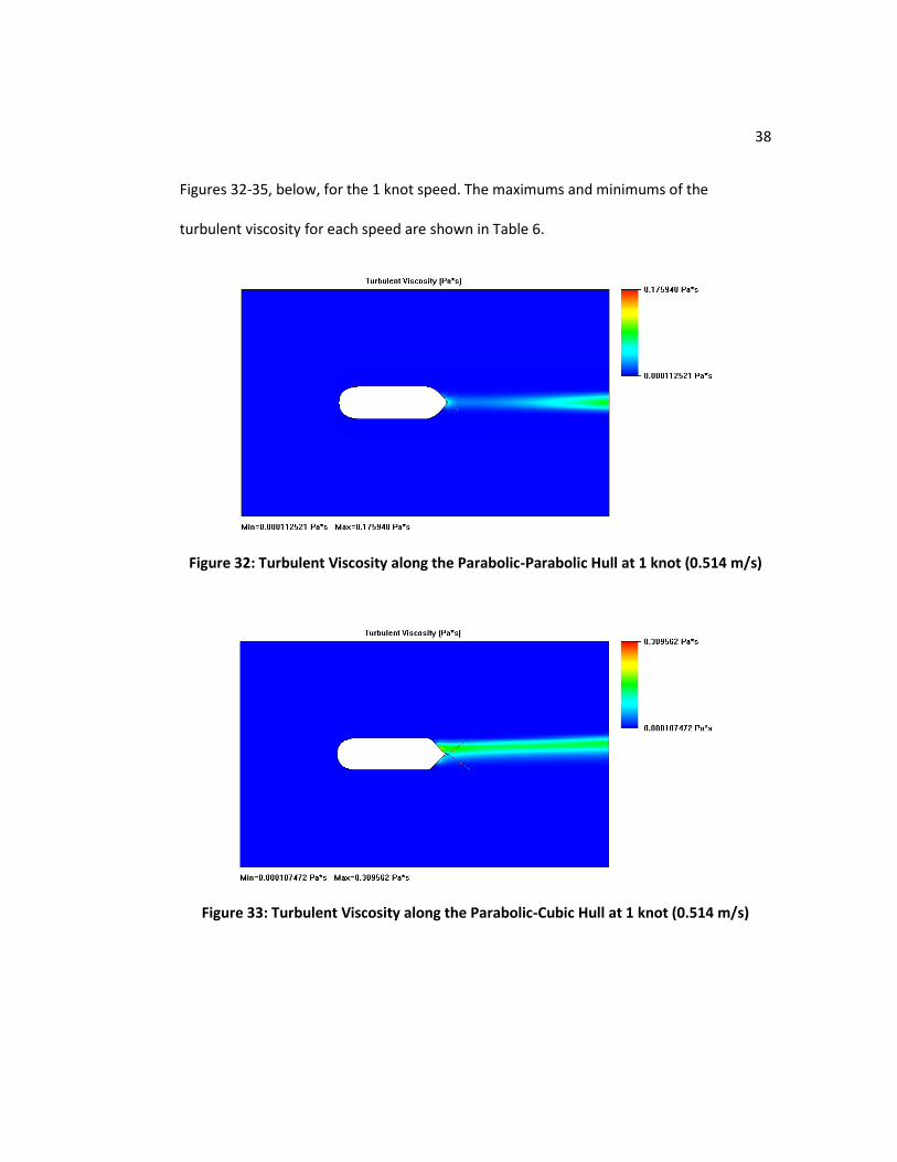
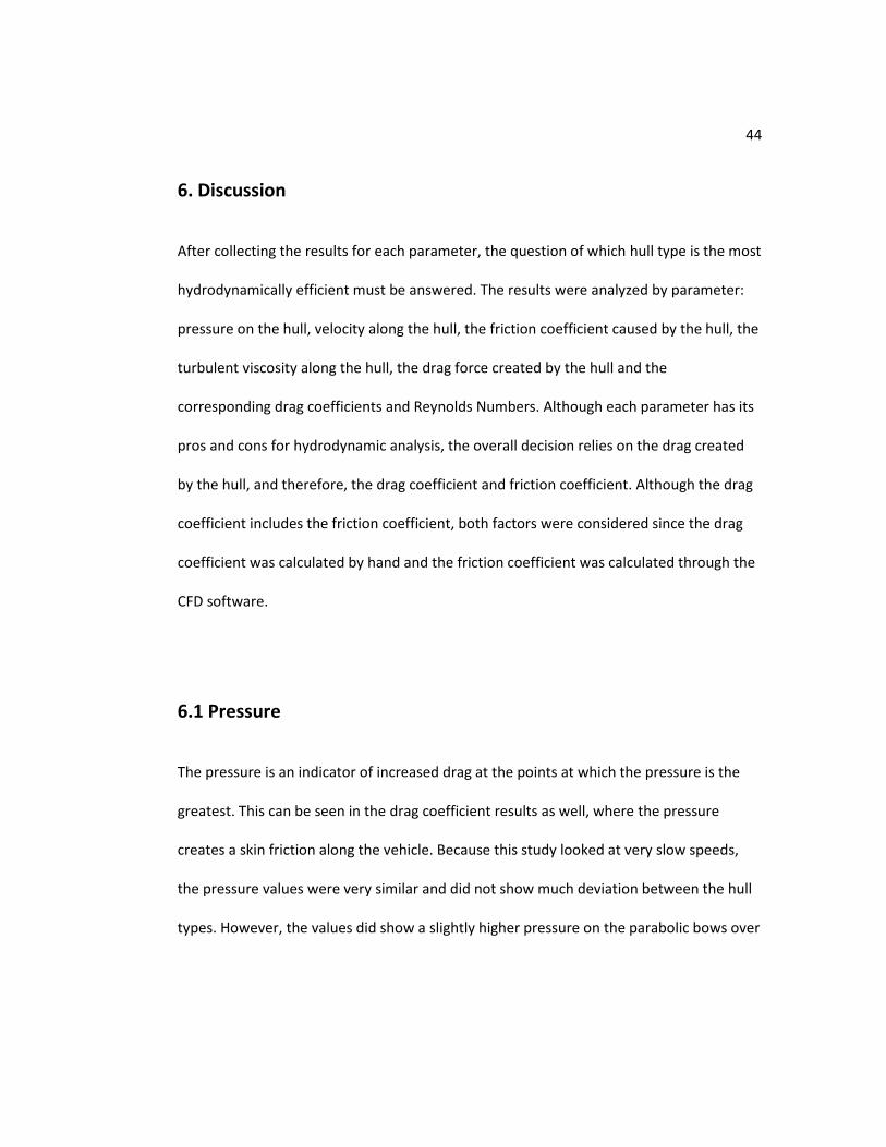
Figures 32-35, below, for the 1 knot speed. The maximums and minimums of the

turbulent viscosity for each speed are shown in Table 6.

Figure 32: Turbulent Viscosity along the Parabolic-Parabolic Hull at 1 knot (0.514 m/s)

Figure 33: Turbulent Viscosity along the Parabolic-Cubic Hull at 1 knot (0.514 m/s)

39

Figure 34: Turbulent Viscosity along the Elliptical-Parabolic Hull at 1 knot (0.514 m/s)

Figure 35: Turbulent Viscosity along the Elliptical-Cubic Hull at 1 knot (0.514 m/s)

40

Table 6: Maximum and Minimum Turbulent Viscosity along all Hull Types at Each Speed

Parabolic-Parabolic Parabolic-Cubic Elliptical-Parabolic Elliptical-Cubic

Velocity (m/s)

Max (Pa·s) Min (Pa·s)

Max (Pa·s) Min (Pa·s)

Max (Pa·s) Min (Pa·s)

Max (Pa·s) Min (Pa·s)

0.0514 0.0224 2.897E-08 0.0400 2.470E-08 0.0264 3.4041E-08 0.0490 4.694E-08

0.2572 0.0629 2.590E-05 0.1760 2.521E-05 0.0837 2.3423E-05 0.1748 3.188E-05

0.514 0.1759 0.0001251 0.3095 0.0001075 0.1254 0.0001067 0.3477 0.0001201

5.5 Drag Force and Drag Coefficient

The drag force values were taken from the global goals in the SolidWorks simulation. The

x-component of force was isolated in order to output the drag force created at each

speed. The drag force compared to the calculated drag coefficients for each vehicle can

be found in Figure 36.

41

Figure 36: Drag Force and Drag Coefficients for each Hull Type

Below, in Table 7, the average drag force and resulting drag coefficient are shown. The

minimum, maximum and averages for each speed can be seen in the Appendix.

Table 7: Drag Force and Drag Coefficient Averages for each Hull Type

FD (N) CD

Parabolic-Parabolic 0.598246 0.013481

Parabolic-Cubic 0.717047 0.015816

Elliptical-Parabolic 0.545189 0.011764

Elliptical-Cubic 0.546429 0.010646

0

0.002

0.004

0.006

0.008

0.01

0.012

0.014

0.016

0.018

0

0.1

0.2

0.3

0.4

0.5

0.6

0.7

0.8

Drag C

oe

fficien

t Dra

g Fo

rce

(N)

FD

CD

42

The resulting calculation of the drag coefficient shows how much that drag force effects

the movement of the hull. In order to decide if the drag coefficient is a significant value,

the differences between each model’s drag force must be shown to be significant. A t-test

was used to find statistical significance at both a 95% confidence level and a 99%

confidence level. As seen below, in Table 8, there was a statistical significance between all

hull types except between the Elliptical-Cubic and Elliptical Parabolic.

Table 8: Statistical Significance of Drag Force between each of the Hull Types

Avg. Fd

(N) Delta Iterations T-score Significant

at 95% Significant

at 99%

Elliptical-Cubic 0.546430 0.007216 288 0.131972 No No

Elliptical-Parabolic 0.545189 0.006025 Elliptical-Cubic 0.546430 0.007216 288 23.256570 Yes Yes

Parabolic-Cubic 0.717048 0.001322 Elliptical-Cubic 0.546430 0.007216 288 6.520815 Yes Yes

Parabolic-Parabolic 0.598247 0.003327 Parabolic-Cubic 0.717048 0.001322 288 27.861070 Yes Yes

Elliptical-Parabolic 0.545189 0.006025 Parabolic-Parabolic 0.598247 0.003327 288 7.708741 Yes Yes

Elliptical-Parabolic 0.545189 0.006025 Parabolic-Cubic 0.717048 0.001322 288 33.180470 Yes Yes

Parabolic-Parabolic 0.598247 0.003327

43

5.6 Reynolds Numbers

The Reynolds Number for each hull was calculated for the 0.1 knot, 0.5 knot, and 1 knot

speeds (0.0514 m/s, 0.2572 m/s, and 0.514 m/s respectively). The results of the

calculations are shown in Figure 37. The lowest Reynolds Numbers belonged to the

Parabolic-Parabolic Hull at 51297, 256687, and 512974 for the 0.1 knot, 0.5 knot and 1

knot speeds, while the highest numbers belonged to the Elliptical-Cubic hull with values

of 56068, 280558, and 560681 at the same speeds.

Figure 37: Reynolds Number for each hull type at each speed

0.00

100000.00

200000.00

300000.00

400000.00

500000.00

600000.00

Ellip-Cub Ellip-Para Para-Cub Para-Para

Reynolds Number

0.0514 m/s

0.2572 m/s

0.514 m/s

44

6. Discussion

After collecting the results for each parameter, the question of which hull type is the most

hydrodynamically efficient must be answered. The results were analyzed by parameter:

pressure on the hull, velocity along the hull, the friction coefficient caused by the hull, the

turbulent viscosity along the hull, the drag force created by the hull and the

corresponding drag coefficients and Reynolds Numbers. Although each parameter has its

pros and cons for hydrodynamic analysis, the overall decision relies on the drag created

by the hull, and therefore, the drag coefficient and friction coefficient. Although the drag

coefficient includes the friction coefficient, both factors were considered since the drag

coefficient was calculated by hand and the friction coefficient was calculated through the

CFD software.

6.1 Pressure

The pressure is an indicator of increased drag at the points at which the pressure is the

greatest. This can be seen in the drag coefficient results as well, where the pressure

creates a skin friction along the vehicle. Because this study looked at very slow speeds,

the pressure values were very similar and did not show much deviation between the hull

types. However, the values did show a slightly higher pressure on the parabolic bows over

45

the elliptical bows. This is logical and expected because the nose of the parabolic bow is

more flattened than that of the elliptical bow. Unfortunately, this was not enough of a

difference to say that the elliptical bows are definitely more hydrodynamic.

6.2 Velocity

The results showed that the Elliptical bow and Cubic tail combination resulted in the

highest maximum velocity around the hull. For this study, the effect on the wings was not

analyzed, however there is a potential for the velocity around the hull to affect the lift on

the wings. The results of the velocity values show how the geometry streamlines through

the water. The better streamlining, the easier it is for the vehicle to move through the

water. Each of the hull types showed the same pattern of increasing in velocity over the

curvature of the bow, and curve of the tail section as well as a decrease in velocity on the

tip of the bow and end of the tail. As previously stated, Myring believed that those bodies

who produce larger velocities tend to produce higher percentages in form drag. The

Parabolic Hulls seemed to have the lowest velocity maximums around the edges, and

therefore may contribute to drag least [13]. However, the similarity of streamlining

throughout each of the hulls, along with the fact that there is no way to pinpoint the

maximum velocity, nor is there a large difference in velocities for each hull, means that

there is no visible benefit of any hull over the others for this parameter.

46

6.3 Friction Coefficient

In this study, the results were based on the average friction coefficients that were found

along the hull for each speed. This represents the boundary layer friction that occurs

along the body. The results show that the Elliptical Bow paired with the Parabolic Tail had

the lowest friction coefficient at each speed, and therefore, the lowest average friction

coefficient. The second lowest values were results of the Parabolic-Parabolic Hull. This

suggests that the Parabolic Tail had the most effect on the friction coefficients. The ITTC-

57 values that were calculated were not comparable to the CFD values. Most likely, this is

due to the fact that the ITTC-57 formula is used mainly for scaled ship models that are

around 2 m in length. The models in this study do not exceed 1.09 m and have fairly low

Reynolds Numbers. The one result that can be considered is the consistency in decreasing

friction coefficient with speed.

6.4 Turbulent Viscosity

The turbulent viscosity shows the overall effect of the geometry of the hull types and

their streamlining. This study took the turbulent viscosity into account in order to see if

the geometry of the bow created any turbulence down the rest of the hull which could

increase the drag on the hull. From the results it can be seen that the Parabolic-Parabolic

Hull had the lowest maximum turbulent viscosities. The differences between the hulls for

47

the minimum values were very small. Overall, the values were too small to provide any

accurate conclusions. Given the precision of the output of the software, it was hard to

determine if there were any changes in turbulence along the cylindrical middle section

which would have affected the drag. It was observed that the wakes created by the

different hulls were very different depending on the tail section and the Parabolic Tails

were seen to create the lowest maximums in turbulent viscosity. This will have an effect

on any additions to the tail sections during future work.

6.5 Drag Force, Drag Coefficient and Reynolds Number

The drag force on the hull was analyzed as the x-component of force along the hull. The

drag coefficient shows the amount that the drag force affects the overall movement of

the hull. The drag coefficient also includes the pressure/form drag. The higher the drag

coefficient, the more effect drag force has over other forces upon movement. As seen in

the results, there was a statistical significance between all hull types except between the

Elliptical-Cubic and Elliptical-Parabolic. This means that the drag force on each hull was

significantly different than the others, with the exception of the Elliptical-Cubic and

Elliptical-Parabolic pair. Interestingly, the lowest drag coefficient of 0.0106 belonged to

the Elliptical-Cubic Hull. This was not expected given that the friction coefficient was the

greatest for the Elliptical-Cubic Hull. The second lowest drag coefficient belonged to the

48

Elliptical-Parabolic Hull, with a value of 0.0118. From this data, the assumption may be

made that the Elliptical Bow has the most influence over the drag coefficient. The

resulting values of the drag coefficient were logically higher than that of a turbulent flat

plate (0.005), but lower than that of a streamlined body (around 0.04). The difference is

most likely due to the fact that this is a fairly small scale study. Going back to the study by

Stevenson et. al, the results for the Laminar Flow Body showed drag coefficients of 0.0109

and 0.013-0.015 for CFD and experimental outcomes respectively, and the NACA airfoils

with similar length to diameter ratios had values of 0.0195-0.025. Given that the AUVs

are moving at over twice the speed and are over twice as large as the gliders in this study,

the values are still very close, and nonetheless shows the importance of the drag on the

hull upon the overall movement of the vehicle.

The Reynolds Number analysis showed that the Parabolic Bow created the lowest values,

with the Parabolic-Parabolic Hull leading the way. This was the result of the difference in

lengths of each hull. Since the volume was kept the same, the length to diameter ratio

became the deciding factor in the resulting Reynolds Number. Therefore, the Elliptical

Bows created higher values.

49

7. Conclusions

The use of SolidWorks Flow Simulation was found to be an effective tool for CFD.

Although it lacks an easy way to incorporate goal equations successfully, simple flow

models could be built with logical parameter outcomes. All of the results gathered were

mathematically logical, matched up to other theoretical standards, and followed the

expected pattern. This would be a good tool for learning about flow, or to get an initial

idea of the flow parameters of a new component, part, or system.

From the results of this study, there was no obvious winner. The friction coefficient

analysis suggests that the Elliptical-Parabolic Hull is the optimum choice with values of

0.0383-0.0113 (at 0.0514 m/s – 0.514 m/s respectively), while the drag coefficient

suggests that the Elliptical-Cubic Hull is the best with an average value of 0.0106. The

values were close to those from other studies; the CFD analysis of the Laminar Flow Body

produced drag coefficients of 0.0109, and the NACA airfoils had values ranging from

0.0195-0.025. The Reynolds Number leans towards the Parabolic-Parabolic Hull as the

best choice (minimum value of 51297), however, the values are very close to each other

and therefore, not valid for comparison. Overall, the Elliptical-Parabolic Hull was either

the best or the second best in each viable analysis, but the results were too close in each

parameter in order to definitively determine which vehicle was the most

50

hydrodynamically efficient. Future work must be done in order to validate the results and

to find the optimal hull design for hydrodynamic efficiency.

51

8. Future Work

This study had a very limited time frame for completion. Thus, there were additions that

were not able to be included. First, the best hull or hulls need to be identified. Evaluating

a change of the length to increase the length to diameter ratio above 4 (lengths of 1.5 m,

1.8m, 2.0 m, etc.), may show a difference in the results that are unique and valid. This

change of dimension could result in changes in the effect of the turbulent viscosity along

the length of the middle section, or the velocity occurring around the hull due to the

geometry. The design of the models in this study could also be compared to some of the

NACA airfoils at the same volumes. To check for validity of SolidWorks as a CFD program

and possibly expose any issues with the gathered values, the models could be input into

different CFD analysis software. Although it may be more time consuming, FLUENT

provides more options for inserting customized fluid equations, therefore increasing the

amount of useful data versus useless output. Once the most hydrodynamically efficient

hulls are chosen, they then can be put through an experimental test.

A good experimental test would be to build the models out of high density foam in a CNC

machine, at a 1/3 to 1/2 scale. The models can then be put through a pulley test in either

a pool or a wave tank. The pull test includes harnessing each model to a fishing line that is

attached to a set of pulleys. One of the pulleys is located in the water at an appropriate

depth such that the entire model will be submerged, and so that the model will not be

52

pulled up out of the water by the second pulley (see Figure 38). The second pulley is

positioned vertically above the pool/tank and leads to the weight. The set weight will

allow the line to pull each model across the pool/tank using equivalent force. A maximum

amount of good repetitions should be obtained for each model. The results can then be

compared to the theoretical values collected in the CFD analysis.

Figure 38: Pulley system for Pull Test

Another way to test this would be to submerge the scaled, or full size models (given the

space is large enough) in an isolated flume. A gauge to read the force could be hooked up

to the nose of the hull and take readings at predetermined speeds. This is a much cleaner

experimental test, but it requires an accurate flume where the speed can be altered as

needed, and large enough to minimize the effects of the outer walls/boundaries.

53

9. References

[1] Applied Physics Laboratory (APL). Seaglider: Summary. n.d.

http://www.apl.washington.edu/projects/seaglider/summary.html

[2] Arima, M., N. Ichihashi and Y. Miwa. 2009. Modelling and Motion Simulation of an Underwater

Glider with Independently Controllable Main Wings. IEEE: OCEANS 2009: Europe. Pp. 1-6.

[3] AUVAC. Slocum Electric Glider Configuration. October 2012.

http://auvac.org/configurations/view/49.

[4] Bluefin Robotics. Spray Glider Product Sheet. 2011.

http://www.bluefinrobotics.com/assets/Downloads/Bluefin-Spray-Glider-Product-

Sheet.pdf

[5] Chui, F., M. Guo, J. Guo, and S. Lee. 2008. Modular modeling of maneuvering motions of an

underwater glider. IEEE: OCEANS 2008. Pp. 1-8.

[6] Davis, R. E., C. C. Eriksen, and C. P. Jones. 2002. Chapter 3: Autonomous buoyancy-driven

underwater gliders. Technology and Applications of Autonomous Underwater Vehicles.

Taylor and Francis, London. Pp. 37-58.

[7] Graver, J.G. 2005. Underwater Gliders: Dynamics, Control and Design. Dissertation, Princeton

University, Department of Mechanical and Aerospace Engineering, May, 2005

[8] Hemmelgarn, R. 2008. Thesis: Development of a Long-Range Gliding Unmanned Underwater

Vehicle Utilizing Java Sun Spot Technology. Naval Post Graduate School: Monterey, CA.

[9] Inoue, T., H. Suzuki, R. Kitamoto, Y. Watanabe and H. Yoshida. 2010. Hull Form Design of

Underwater Vehicle Applying CFD (Computational Fluid Dynamics). OCEANS 2010 IEEE –

Sydney. Pp 1-5.

[10] Isa, K. and M.Arshad. 2011. Dynamic Modeling and Characteristics Estimation for USM

Underwater Glider. IEEE Control and System Graduate Research Colloquium. Pp. 12-17.

54

[11] Jones, A., Ph.D. Candidate in Ocean Engineering. Personal Interview. September 10, 2012.

[12] Kawaguchi, K., T. Ura, Y. Tomoda, Y. Kobayashi. 1993. Development and Sea Trials of a Shuttle

Type AUV "ALBAC". Proc. 8th. Intn. Symp. on Unmanned Untethered Submersible

Techonology. Durham, Sep. 1993. Pp.7-13.

[13] Myring, D.F. 1976. A Theoretical Study of Body Drag in Subcritical Axisymmetric Flow.

Aeronautical Quarterly. Pp. 186-194.

[14] National Marine Facilities: USL. Autosub. October 2012.

http://www.noc.soton.ac.uk/nmf/usl_index.php?page=as

[15] NURC. Autonomous Underwater Vehicles. October 2012.

http://www.uncw.edu/nurc/AUV/glider/about.htm

[16] Osse, T. and C. Erikson. 2007. The Deepglider: A Full Ocean Depth Glider for Oceanographic

Research. IEEE: OCEANS 2007. Pp. 1-12.

[17] Phillips, A., M. Furlong, and S.R. Turnock. 2007. The Use of Computational Fluid Dynamics to

Assess the Hull Resistance of Concept Autonomous Underwater Vehicles. IEEE: OCEANS

2007: Europe. Pp. 1-6.

[18] Sagala F. and R. Bambang. 2011. Development of Sea Glider Autonomous Underwater Vehicle

Platform for Marine Exploration and Monitering. Indian Journal of Geo Marine Sciences:

Vol. 40, N. 2. Pp. 287-295.

[19] Sherman, J., Davis, R. E., Owens, W. B., and Valdes, J. (2001). “The autonomous

underwaterglider Spray,” IEEE J. Oceanic Engineering., Volume 26, Issue 4, Oct. 2001, pp.

437-446.

[20] Shultz, M.P., J.A. Finlay, M.E. Callow and J.A. Callow. 2003. Three Models to Relate

Detachment of Fouling at Laboratory and Ship Scale. Biofouling: Vol. 19. Pp 17-26.

55

[21] Stevenson P., M. Furlong, and D. Dormer. 2007. AUV shapes - Combining the Practical and

Hydrodynamic Considerations. OCEANS 2007 – Europe. Pp. 1-6.

[22] StarStat: Significance Testing Calculator. DataStar, Inc. 10 November 2012.

http://www.surveystar.com/our_services/ttest.htm

[23] Teledyne-Webb. G2 Slocum Glider Datasheet. 2010.

http://www.webbresearch.com/pdf/Slocum_Glider_Data_Sheet.pdf

[24] Triantafyllou, M. S., and F. Hover. 2002. Maneuvering and Control of Marine Vehicles.

Department of Ocean Engineering Massachusetts Institute of Technology: Cambridge,

Massachusetts USA. Pp. 62.

[25] Wang Y., Y. Wang and Z. He. 2011. Bouyancy compensation analysis of an autonomous

underwater glider. IEEE: 2011 International Conference on Electronic & Mechanical

Engineering and Information Technology. Pp. 824-827.

[26] Webb, D. C., P.J. Simonetti, C.P. Jones. 2001. SLOCUM: an underwater glider propelled by

environmental energy. IEEE J. Oceanic Engineering. Volume 26, Issue 4, Oct. 2001. Pp. 447

– 452.

[27] Wolk, F., R.G. Lueck, and L.St. Laurent. 2009. Turbulence Measurements from a Glider.

OCEANS 2009, MTS/IEEE Biloxi - Marine Technology for Our Future: Global and Local

Challenges. Pp 1-6.

.

56

10. Appendix

Table 9: Drag Force Maximums, Minimums and Averages, Standard Deviations, Reynolds Number

and Drag Coefficients

Elliptical-Cubic

Velocity (m/s)

Averaged Value (N)

Minimum Value (N)

Maximum Value (N) Delta

Average Fd (N)

Average Delta

Reynolds Number

0.0514 0.013923440 0.013786289 0.013961471 0.000175182 56068.06

0.2572 0.330885410 0.328018828 0.332398890 0.004380061 0.546429970 0.007216211 280558.48

0.5140 1.294481060 1.284092749 1.301186140 0.017093391 560680.64

Coefficient

of Drag Averaged

Value Minimum

Value Maximum

Value

Average Cd

0.0514 0.011094985 0.010985695 0.011125290

0.2572 0.010530332 0.010439104 0.010578498 0.010646825

0.5140 0.010315157 0.010232377 0.010368587

Elliptical-Parabolic

Velocity (m/s)

Averaged Value (N)

Minimum Value (N)

Maximum Value (N) Delta

Average Fd (N)

Average Delta

Reynolds Number

0.0514 0.017788016 0.017719529 0.017854422 0.000134893 54375.25

0.2572 0.344856297 0.342667304 0.346176173 0.003508869 0.545189333 0.006025057 272087.82

0.5140 1.272923686 1.264324173 1.280799139 0.014431410 543752.50

Coefficient

of Drag Averaged

Value Minimum

Value Maximum

Value

Average Cd

0.0514 0.014174497 0.014119923 0.014227413

0.2572 0.010974952 0.010905288 0.011016956 0.011764275

0.5140 0.010143376 0.010074850 0.010206132

57

Table 9: Drag Force Maximums, Minimums and Averages, Standard Deviations, Reynolds

Number and Drag Coefficients Continued… Parabolic-Cubic

Velocity (m/s)

Averaged Value (N)

Minimum Value (N)

Maximum Value (N) Delta

Average Fd (N)

Average Delta

Reynolds Number

0.0514 0.021694673 0.021632792 0.021764227 0.000111764 52990.22

0.2572 0.448324329 0.445564460 0.449287734 0.003723274 0.717047877 0.001322158 265157.29

0.5140 1.681124630 1.672155211 1.686192786 0.000131435 529902.20

Coefficient

of Drag Averaged

Value Minimum

Value Maximum

Value

Average Cd

0.0514 0.018247962 0.018195912 0.018306466

0.2572 0.015060447 0.014967736 0.015092811 0.015816264

0.5140 0.014140383 0.014064938 0.014183012

Parabolic-Parabolic

Velocity (m/s)

Averaged Value (N)

Minimum Value (N)

Maximum Value (N) Delta

Average Fd (N)

Average Delta

Reynolds Number

0.0514 0.019079249 0.019061518 0.019092728 3.12097E-05 51297.41

0.2572 0.375730320 0.373709159 0.376151761 0.002442602 0.598246955 0.003327391 256686.63

0.5140 1.399931294 1.394255457 1.401763817 0.00750836 512974.05

Coefficient

of Drag Averaged

Value Minimum

Value Maximum

Value

Average Cd

0.0514 0.016048060 0.016033146 0.016059397

0.2572 0.012621815 0.012553918 0.012635972 0.013481689

0.5140 0.011775191 0.011727450 0.011790605