A Computational Approach to Simulating the Performance of

Wright State University Wright State University

CORE Scholar CORE Scholar

Browse all Theses and Dissertations Theses and Dissertations

2013

A Computational Approach to Simulating the Performance of a A Computational Approach to Simulating the Performance of a

24-Hour Solar-Fuel Cell-Hydrogen Electric Power Plant 24-Hour Solar-Fuel Cell-Hydrogen Electric Power Plant

Michael K. Gustafson Wright State University

Follow this and additional works at: https://corescholar.libraries.wright.edu/etd_all

Part of the Mechanical Engineering Commons

Repository Citation Repository Citation Gustafson, Michael K., "A Computational Approach to Simulating the Performance of a 24-Hour Solar-Fuel Cell-Hydrogen Electric Power Plant" (2013). Browse all Theses and Dissertations. 788. https://corescholar.libraries.wright.edu/etd_all/788

This Thesis is brought to you for free and open access by the Theses and Dissertations at CORE Scholar. It has been accepted for inclusion in Browse all Theses and Dissertations by an authorized administrator of CORE Scholar. For more information, please contact [email protected].

https://corescholar.libraries.wright.edu/

https://corescholar.libraries.wright.edu/etd_all

https://corescholar.libraries.wright.edu/etd_comm

https://corescholar.libraries.wright.edu/etd_all?utm_source=corescholar.libraries.wright.edu%2Fetd_all%2F788&utm_medium=PDF&utm_campaign=PDFCoverPages

http://network.bepress.com/hgg/discipline/293?utm_source=corescholar.libraries.wright.edu%2Fetd_all%2F788&utm_medium=PDF&utm_campaign=PDFCoverPages

https://corescholar.libraries.wright.edu/etd_all/788?utm_source=corescholar.libraries.wright.edu%2Fetd_all%2F788&utm_medium=PDF&utm_campaign=PDFCoverPages

mailto:[email protected]

i

A Computational Approach to

Simulating the Performance of a

24-Hour Solar-Fuel Cell-Hydrogen

Electric Power Plant

A thesis submitted in partial fulfillment

of the requirements for the degree of

Master of Science in Engineering

By

Michael K. Gustafson

B.S.Ch.E., Iowa State University, 2010

2013

Wright State University

ii

WRIGHT STATE UNIVERSITY

SCHOOL OF GRADUATE STUDIES

May 27, 2013

I HEREBY RECOMMEND THAT THE THESIS PREPARED UNDER MY SUPERVISION BY

Michael K. Gustafson ENTITLED A Computational Approach to Simulating the Performance of

a 24-Hour Solar-Fuel Cell-Hydrogen Electric Power Plant BE ACCEPTED IN PARTIAL

FULFILLMENT OF THE REQUIREMENTS FOR THE DEGREE OF Master of Science in

Engineering.

________________________________

James Menart, Ph.D.

Thesis Director

________________________________

Hong Huang, Ph.D.

Thesis Director

________________________________

George Huang, Ph.D.

Chair

Department of Mechanical and Materials Engineering

________________________________

R. William Ayres, Ph.D.

Interim Dean

Graduate School

Committee on Final Examination

___________________________

James Menart, Ph.D.

___________________________

Hong Huang, Ph.D.

___________________________

Amir Farajian, Ph.D.

iii

Abstract Gustafson, Michael K. M.S.Egr., Department of Mechanical and Materials Engineering,

Wright State University, 2013.

A Computational Approach to Simulating the Performance of a 24-Hour Solar-Fuel

Cell-Hydrogen Electric Power Plant

World energy demand has risen from about 375 exajoules (EJ) in 1990 to around 600 EJ

today. The Energy Information Administration predicts that by the year 2035, this figure will

rise to around 800 EJ [EIA (2011)]. This places large stresses on the electric generation

infrastructure. Increasingly this demand is being met by renewable energy sources. There are

several reasons this is the case. The prices of renewables are dropping quickly and reaching

grid parity in more regions. Utilizing renewable energy generation can help achieve energy

security: adverse weather or military conflicts are less likely to impact supply routes when

energy is produced closer to home. Furthermore, renewable energy technologies are

attractive because they do not adversely affect the environment by releasing greenhouse

gases which contribute to global warming.

One major problem with the deployment of renewable technologies is their intermittent

nature. In order to achieve good market penetration it is likely that some sort of energy

storage needs to be employed. Several types exist such as thermal storage, pumped storage,

batteries and chemicals. Chemical energy derived from renewables is attractive because it

has long storage lifetimes, is easily transportable and can be produced from abundant

feedstocks; as in the case of generating hydrogen from water electrolysis. Hydrogen

produced from solar energy shows promise because of the abundant feedstock (water) and

energy supply (the sun). One way that hydrogen can be used to buffer the intermittent nature

of solar energy is by using photovoltaic modules to produce electricity which is used to

electrolyze water with a regenerative fuel cell and then storing the hydrogen gas. Small-scale

solar-fuel cell-hydrogen power plants have been constructed and tested, but often suffer from

poor equipment reliability or improper equipment sizing. More study on the effects of

component sizing on the system performance of these power plants must be performed.

iv

In this research, a computer program is developed which can simulate the long-term behavior

of a solar-fuel cell-hydrogen power plant given any sizing of system components: the number

and type of photovoltaic modules, the total power of the regenerative fuel cells and the

hydrogen storage capacity. Taking into account the details of the system components,

location of the plant, meteorological data and the demand load, this program predicts the

behavior of such a power plant for any time period. In particular the program can be used to

simulate time periods that eliminate the effect of the plant start-up. In essence this is done by

running the program for several years to remove the effects of the initial conditions. The

biggest initial condition that affects short term results is the amount of hydrogen in storage at

the beginning of the simulation. Another important aspect of this program is that the

simulation is done on an hourly basis. This computer program outputs important parameters

such as how much of the electricity demand was met, how much excess electricity was

produced, the amount of solar resource available, the power output of the photovoltaic array,

the power into or out of the regenerative fuel cell, and the amount of hydrogen in storage.

From these outputs, the proper sizing of a solar-fuel cell-hydrogen power plant can be

determined for any size load from residential to utility-scale.

v

Table of Contents Abstract ..................................................................................................................................... iii

Table of Contents ....................................................................................................................... v

List of Figures and Tables........................................................................................................ vii

Chapter 1 – Introduction ........................................................................................................... 1

1.1. Why Use Renewable Energy? ............................................................................... 1

1.2. Objectives of Project .............................................................................................. 5

Chapter 2 – Literature Review of Solar-Fuel Cell- Hydrogen Power Plant Systems ............... 6

2.1. General Literature .................................................................................................. 6

2.2. PHOEBUS Demonstration Plant ........................................................................... 7

2.3. Solar Wasserstoff-Bayern System ....................................................................... 11

2.4. Helsinki Hydrogen Energy Project ...................................................................... 12

2.5. Schatz Solar Hydrogen Project ............................................................................ 13

2.6. ENEA SAPHYS: Stand-Alone Small Size Photovoltaic Hydrogen Energy

System ......................................................................................................................... 14

2.7. Summary .............................................................................................................. 15

Chapter 3 - Photovoltaics ........................................................................................................ 16

3.1. The Photovoltaic Effect ....................................................................................... 16

3.2. Modeling Photovoltaic Devices ........................................................................... 18

3.3. Effects of Solar Irradiance and Temperature ....................................................... 26

Chapter 4 – Modeling the Solar Resource .............................................................................. 30

4.1. Extraterrestrial Solar Resource ............................................................................ 30

4.2. Terrestrial Effects on the Solar Resources ........................................................... 31

Chapter 5 – Fuel Cells............................................................................................................. 37

5.1. Fuel Cell Operation Theory ................................................................................. 37

5.2. Modeling the Operation of a Regenerative Fuel Cell .......................................... 39

5.3. Fuel Cell Efficiency ............................................................................................. 47

Chapter 6 – Hydrogen Storage ................................................................................................ 52

6.1. Modeling Hydrogen Storage ................................................................................ 52

Chapter 7 – Computer Program .............................................................................................. 58

7.1. Running the Program ........................................................................................... 58

7.2. Program Operation ............................................................................................... 66

vi

7.3. Program Outputs .................................................................................................. 68

7.4. Running Multiple Results Simultaneously .......................................................... 72

Chapter 8 – Component Sizing ............................................................................................... 74

8.1. Microscale Phenomena ........................................................................................ 74

8.2. Macroscale Phenomena ....................................................................................... 79

Chapter 9 – House Size Demand Load Results ...................................................................... 82

9.1. eQUEST House Specifications ............................................................................ 82

9.2. House Size Demand - Results .............................................................................. 86

Chapter 10 – Effects of Fuel Cell Size on System Performance ............................................ 97

Chapter 11 – Utility Size Demand Load Results .................................................................. 103

Chapter 12 – Summary and Conclusions .............................................................................. 112

References ............................................................................................................................. 117

Appendix A – Tabulated Results for Residential, Baseload and Utility Load Studies......... 120

Appendix B – Graphical Results for Residential Load Studies ............................................ 131

vii

List of Figures and Tables Figure 1.1: Schematic diagram for a solar-fuel cell-hydrogen electric power plant. ............... 4

Table 2.1: System component specifications for selected solar-fuel cell-hydrogen systems. .. 7

Figure 2.1: The PV array on top of the Central Library [Ghosh et al. (2003)]. ........................ 8

Figure 2.2: The 26 kW electrolyzer used in the PHOEBUS demonstration plant [Ghosh et al.

(2003)]....................................................................................................................................... 8

Figure 2.3: The 5 kW PEMFC stack used in the ...................................................................... 9

demonstration plant [Ghosh et al. (2003)]. ............................................................................... 9

Figure 2.4: Diagram for the PHOEBUS demonstration plant [Ghosh et al. (2003)]. ............. 10

Figure 2.5: Hydrogen production and consumption for the PHOEBUS plant [Ghosh et al.

(2003)]..................................................................................................................................... 11

Figure 2.6: Schematic diagram for the Helsinki demonstration plant [Vanhanen (1997)]. .... 13

Figure 3.1: Simplified diagram of typical PV cell components.............................................. 16

Figure 3.2: Equivalent circuit of a PV cell. ............................................................................ 18

Figure 3.3: Equivalent circuit of a PV cell with an infinite shunt resistance .......................... 21

Figure 3.4: Operating curves for a PV module showing current vs. voltage (I-V) and power

vs. voltage (I-P). ..................................................................................................................... 26

Figure 3.5: Effects of solar irradiance (S) on the I-V curve of a typical PV module where

T=298K. .................................................................................................................................. 27

Figure 3.6: Effects of temperature on the I-V curve of a typical module with S=1000W/m2. 27

Table 3.1: Empirical coefficients for use in Eqns. 3.26 and 3.27 [King et al. (2003)]. .......... 29

Figure 4.1: Variation in extraterrestrial solar radiation with the day of the year.................... 31

Table 4.1: Brightness coefficients from Perez et al. (1988). .................................................. 36

Table 5.1: Some common fuel cell type specifications [Fuel Cell Fundamentals (2009)]. .... 38

Figure 5.1: Diagram of a SOFC and its chemical species flows. ........................................... 40

Figure 5.2: Fuel cell j-V curve generated using Eqn. 5.17. The power curve is also shown. . 46

Figure 5.3: Electrolysis mode j-V curve generated using Eqn. 5.19. The power curve is also

shown. ..................................................................................................................................... 47

Figure 5.3: Efficiency curves for both constant stoichiometry and constant flow rate

conditions. For constant stoichiometry =1 and for constant flow rate, 1.1 times the required

flow rate at maximum current is supplied. .............................................................................. 49

Figure 6.1: Compressibility factors for hydrogen vs. temperature and pressure [Klell (2010)].

................................................................................................................................................. 55

Figure 6.2: Conversion chart between kilograms of hydrogen and volume, given a 50 bar

storage tank. ............................................................................................................................ 57

Figure 7.1: Initial GUI upon running the MATLAB code. ..................................................... 59

Figure 7.2: Location selection GUI. ....................................................................................... 59

Figure 7.3: Demand load specification GUI. .......................................................................... 60

Figure 7.4: Photovoltaic array design GUI. ............................................................................ 62

Figure 7.5: Regenerative fuel cell design GUI. ...................................................................... 64

Figure 7.6: Hydrogen storage capacity GUI. .......................................................................... 65

Figure 7.7: GUI for system start time and run time. ............................................................... 65

Figure 7.8: System performance output screen (Run time ~= 7 months) ............................... 69

viii

Figure 7.9: System performance output screen zoomed in. .................................................... 71

Figure 7.10: Example of MATLAB command line outputs. .................................................. 71

Figure 7.11: Screenshot of the “Automation.m” file for running multiple results. ................ 72

Figure 8.1: A properly sized system. ...................................................................................... 76

Figure 8.2: A system with too large of a PV array. ................................................................ 76

Figure 8.3: A system with too small of a PV array. ................................................................ 77

Figure 8.4: A system with too small of a hydrogen tank. ....................................................... 77

Figure 8.5: A system with too small of a fuel cell. ................................................................. 78

Figure 8.6: A system that is adequately sized. ........................................................................ 80

Figure 8.7: A system that is sized too small. .......................................................................... 80

Figure 8.8: A system that is sized too large. ........................................................................... 81

Table 9.1: Some of the base house specifications used in the eQUEST simulation. .............. 83

Figure 9.1: Schematic of the base house. ................................................................................ 84

Table 9.2: Some of the efficient house specifications used in the eQUEST simulation. ....... 86

Figure 9.2: Schematic of the efficient house. ......................................................................... 86

Figure 9.3: Base house electric demand for Dayton, OH. ...................................................... 87

Figure 9.4: Efficient house electric demand for Dayton, OH. ................................................ 88

Figure 9.5: Base house electric demand for Yuma, AZ. ......................................................... 88

Figure 9.6: Efficient house electric demand for Yuma, AZ. .................................................. 89

Table 9.3: Electric demand properties for both houses in Dayton and Yuma. ....................... 89

Figure 9.7: System performance for the efficient house in Yuma, AZ for seven years of

operation with 54 PV modules, a 20 kW fuel cell and 25 kg hydrogen storage. All of the

demand is met. ........................................................................................................................ 90


operation with 45 PV modules, a 20 kW fuel cell and 25 kg hydrogen storage. About 96% of

the demand is met. .................................................................................................................. 91

Figure 9.9: System performance for the efficient house in Dayton, OH for seven years of


demand is met. ........................................................................................................................ 91


operation with 88 PV modules, a 20 kW fuel cell and 25 kg hydrogen storage. About 90% of

the demand is met. .................................................................................................................. 92

Figure 9.11: Percentage of demand met vs. component sizes for base house in Dayton, OH.

................................................................................................................................................. 93

Figure 9.12: Percentage of demand met vs. component sizes for efficient house in Dayton,

OH. .......................................................................................................................................... 93

Figure 9.13: Percentage of demand met vs. component sizes for base house in Yuma, AZ. . 94

Figure 9.14: Percentage of demand met vs. component sizes for efficient house in Yuma, AZ.

................................................................................................................................................. 94


methods. For constant stoichiometry =1 and for constant flow rate, 1.1 times the required

flow rate at maximum current density is supplied. ................................................................. 98

Figure 10.2: System performance curves using a 2.5 kW fuel cell, 55 PV modules and 25 kg

of hydrogen storage. Run time is seven years......................................................................... 98

ix

Figure 10.3: System performance curve using a 5 kW fuel cell, 55 PV modules and 25 kg of

hydrogen storage. Run time is seven years. ............................................................................ 99

Figure 10.4: System performance curve using a 10 kW fuel cell, 55 PV modules and 25 kg of

hydrogen storage. Run time is seven years. ............................................................................ 99

Figure 10.5: Percentage of demand met vs. different component sizes for a 2.5 kW fuel cell.

............................................................................................................................................... 101

Figure 10.6: Percentage of demand met vs. different component sizes for a 5 kW fuel cell.

............................................................................................................................................... 101

Figure 10.7: Percentage of demand met vs. different component sizes for a 10 kW fuel cell.

............................................................................................................................................... 102

Figure 11.1: Demand curve for Dayton Power and Light. ................................................... 103

Figure 11.2: Percentage of demand met vs. system component sizes in Dayton, OH using a 5

GW fuel cell. ......................................................................................................................... 104

Figure 11.3: Percentage of demand met vs. system component sizes when the PV array is

located in Yuma, AZ and the fuel cell system and hydrogen storage tank are placed in

Dayton, OH. A 5 GW fuel cell is used. ................................................................................ 105

Figure 11.4: Percentage of demand met vs. system component sizes in Dayton, OH using a

25 GW fuel cell. .................................................................................................................... 106

Figure 11.5 Percentage of demand met vs. system component sizes when the PV array is


Dayton, OH. A 25 GW fuel cell is used. .............................................................................. 107

Figure 11.6: System performance when the PV array is located in Yuma, AZ and the fuel cell

system and hydrogen storage tank are placed in Dayton, OH. A 25 GW fuel cell is used along

with 2 million kg of hydrogen storage and 25 million PV modules. This system is clearly

undersized with just 72.7% of the demand met. Run time is seven years. ........................... 109



with 2 million kg of hydrogen storage and 190 million PV modules. This system is oversized

because the demand can be met with fewer panels (See Figure 11.8) and the electricity

surplus can be reduced. Run time is seven years. ................................................................. 109



with 2 million kg of hydrogen storage and 115 million PV modules. This system is properly

sized with 100% of the demand met. Run time is seven years. ............................................ 110

Figure 11.9: System performance when the system is placed in Dayton, OH. A 25 GW fuel

cell is used along with 2 million kg of hydrogen storage and 65 million PV modules. This

system is clearly undersized with 88.8% of the demand met. Run time is seven years. ...... 110



system is slightly undersized with 98.9% of the demand met. Run time is seven years. ..... 111



system is properly sized with 100% of the demand met. Run time is seven years. .............. 111

Table A1: Yuma, AZ - 2 kW constant load- 2.5 kW fuel cell (7 years). .............................. 120

Table A2: Yuma, AZ - 2 kW constant load - 5 kW fuel cell (7 years). ............................... 121

x

Table A3: Yuma, AZ - 2 kW constant load - 10 kW fuel cell (7 years). .............................. 122

Table A4: Dayton, OH – Base house load – 20 kW Fuel cell (7 years). .............................. 123

Table A5: Dayton, OH – Efficient house load – 20 kW Fuel cell (7 years). ........................ 124

Table A6: Yuma, AZ – Base house load – 20 kW Fuel cell (7 years).................................. 125

Table A7: Yuma, AZ – Efficient house load – 20 kW Fuel cell (7 years). .......................... 126

Table A8: Dayton, OH – DPL load – 5 GW Fuel cell (7 years). .......................................... 127

Table A9: Dayton, OH – DPL load – 25 GW Fuel cell (7 years). ........................................ 128

Table A10: Yuma, AZ – DPL load – 5 GW Fuel cell (7 years). .......................................... 129

Table A11: Yuma, AZ – DPL load – 25 GW Fuel cell (7 years). ........................................ 130

Figure B1: System performance for the efficient house in Dayton, OH for seven years of

operation with 60 PV modules, a 20 kW fuel cell and 25 kg hydrogen storage. .................. 131


operation with 60 PV modules, a 20 kW fuel cell and 50 kg hydrogen storage. .................. 131


operation with 60 PV modules, a 20 kW fuel cell and 100 kg hydrogen storage. ................ 132


operation with 60 PV modules, a 20 kW fuel cell and 200 kg hydrogen storage. ................ 132

1

Chapter 1 – Introduction 1.1. Why Use Renewable Energy?

World energy demand has risen from about 375 EJ in 1990 to around 600 EJ today. The

Energy Information Administration estimates that this figure will rise to about 800 EJ by

2035 [EIA (2011)]. This rapidly growing energy demand places huge pressures on the

electric generation infrastructure. In response, new generating capacity must be added.

Increasingly, this new generating capacity is being met with renewable forms of generation

such as solar, wind, geothermal, tidal, etc. In the future, the share of electric generation by

renewables is expected to increase even further. There are many reasons for this.

1) Several renewable technologies, such as solar and wind, are maturing quickly and

reaching grid parity in more and more regions. For example, in the 1950s, the first

silicon solar photovoltaic cells cost around $200/watt, but have since dropped to

below $1/W [Nelson (2004)]. In some regions solar photovoltaics are already

generating electricity at lower costs than conventional sources such as coal. As these

technologies mature and drop in price, their deployment should become even more

widespread as grid parity is attained in more regions.

2) Renewable technologies can aid in achieving energy security. In the United States, a

great portion of the petroleum products that are consumed are imported from other

countries. Disruptions such as natural disasters or military conflicts could disrupt

supply routes leading to temporary energy deficits until other sources of supply can

be secured. By utilizing renewable technologies for energy generation, disruptions

become less likely as the energy is produced within the country, closer to where it is

consumed.

2

3) Environmental factors also play a significant role in driving the growth of renewable

generating capacity. Conventional energy sources are proving to have deleterious

effects on the environment. All fossil fuels, once combusted, release greenhouse

gases into the environment. These gases absorb and reemit some thermal radiation

from the Earth that would otherwise escape into space. This causes the Earth to heat

more than if these gases were not present in their current concentrations. Before the

industrial revolution, the concentration of CO2 in the atmosphere varied between 200

and 300 ppm. Since the industrial revolution, this number has risen to about 400 ppm.

If fossil fuels continue to be utilized at their current rates, this number is expected to

rise even further, which may continue the trend of global warming, accelerating

climate change. Some of the effects of continued global warming include melting of

the polar ice caps, a raise in the ocean levels, and severe weather including droughts

and more frequent, stronger storms. These effects may cause significant economic

loss. For these reasons, cleaner forms of energy generation are sought. Many

renewable technologies release no greenhouse gases nor cause significant

environmental harm. If clean technologies are favored over more damaging ones, the

threat of global warming and climate change may be mitigated.

One further consideration in choosing renewable technologies for energy generation is the

future growth prospects of different forms of energy. In order to match the growing future

energy demands, successful technologies will be ones that are able to grow along with these

demands. While fossil fuels may be able to meet today‟s demands, the fact that they are finite

resources ultimately hinders their future potential. Solar, on the other hand, is Earth‟s most

abundant energy resource. About one and a half hours of solar radiation reaching Earth‟s

surface is enough to meet the world‟s energy demand for one year [Tsao, (2006)]. This

demonstrates solar energy‟s potential to keep up with a growing demand.

While renewable technologies may have the potential to meet growing energy demands and

mitigate environmental damage, their deployment in the future may be hindered by their

intermittent nature. If the sun is not shinning or the wind not blowing, energy cannot be

3

harvested for consumption. This is problematic, as energy is demanded “round the clock” by

consumers. Backup generation, often in the form of fossil fuels, is therefore required.

One solution to the intermittent nature of renewable energy is to use some type of energy

storage as a buffer. Many different types exist such as thermal storage, pumped storage,

batteries or chemical storage. Each of these has its own unique set of challenges. Thermal

storage has limited storage times because heat naturally leaves the system. Also, its

conversion efficiency is Carnot limited. Pumped storage is limited to certain areas where

natural reservoirs exist at different elevations. Batteries, at the moment, are often heavy and

bulky while possessing relatively short lifetimes. Furthermore, of these three forms, none of

them are very transportable.

Chemical energy storage has strong potential for many reasons. Theoretically, chemical

storage has very long storage times as contrasted with thermal energy storage. It is not

limited to areas with proper gravitational gradients like those that are required for pumped

storage. Chemical storage need not be heavy or bulky like batteries. Furthermore, in practice

it can be easily transportable depending on the types of chemicals used. Integrating chemical

storage from renewable sources into the existing infrastructure may not require a complete

reworking of the infrastructure; it is already set up to transport energy stored in chemicals,

e.g. natural gas and oil pipelines, tank farms, chemical tankers, tank trucks, etc.

Many different types of chemical energy storage exist. Excess energy from renewable

sources can be stored as hydrogen, ammonia, hydrazine, methane, ethane, etc. In order to

create these chemicals, different feedstocks are required. For example, in order to generate

methane, carbon dioxide and hydrogen are required. To make ammonia, nitrogen and

hydrogen are required. In order to make hydrogen, only water is required. Because of its

abundance, low cost and safety, water is an ideal feedstock for storing energy generated by

renewable sources. Once hydrogen is generated it can either be stored in its pure form or

used as a reactant to generate other chemicals and compounds.

4

Generating hydrogen from water and renewable energy is both a renewable and clean

process. In one cycle of splitting water to form hydrogen, storing it and then reacting it with

oxygen to form water again, no water is consumed or destroyed. In this way, hydrogen power

using renewable energy can act as an inexhaustible fuel supply, able to scale to the extremely

large energy demands of the future.

One way to generate hydrogen for use as a buffer to the intermittent nature of renewables is

to use the electricity derived from solar photovoltaics along with regenerative fuel cells to

split water. The hydrogen can then be stored and when electricity is demanded, run back

through the fuel cell along with environmental oxygen to form water and electricity. A

simplified schematic of this type of power plant is shown in Figure1.1.

Figure 1.1: Schematic diagram for a solar-fuel cell-hydrogen electric power plant.

5

1.2. Objectives of Project

In order to determine the long term performance of solar-fuel cell-hydrogen power plants, a

computer model is developed that accurately models the behavior of each system component

during the operation of the plant. Using this model, the performance of the power plant will

be calculated hourly over a specified run time. The significant inputs are the specifications of

the system components, the location of the plant, meteorological data, and electricity demand

data.

The program will calculate on an hourly basis the performance of each component and the

total system behavior. The outputs of the program that are of great significance are the power

output of the PV array, the power into or out of the regenerative fuel cell, the hydrogen

storage tank levels, the system level energy deficits and surpluses, and the percentage of

demand that was met. From these results, the inputs can be refined until the solar-fuel cell-

hydrogen power plant is sized properly to meet all of the electric demand. This thesis will

present the theory upon which this new computer simulation model is based, many results

from this model, and insights into the sizing of such systems. It needs to be said that the

purpose of this research is not to present cost or payback period information on such systems.

To build a 24 hour solar-fuel cell-hydrogen power plant would be expensive currently.

Costing information will have to be the subject of future research; however, the computer

model developed as part of this thesis is absolutely essential to doing a detailed economic

analysis. This computer model can also be used to test several ideas for reducing the cost of

such a system.

6

Chapter 2 – Literature Review of Solar-Fuel Cell-

Hydrogen Power Plant Systems The following review gives a brief overview on the experimental solar-fuel cell-hydrogen

energy systems as documented in the literature. This review does not go into great detail as

far as theoretic modeling is concerned. This is left to the following chapters which outline the

theory behind the operation of photovoltaics, fuel cells and hydrogen storage. Several small-

scale (a few kW) power plant systems have been designed over the last couple of decades

with the late 1980s and early 1990s generally regarded as the start of this type of research on

solar-fuel cell-hydrogen systems. At this point in time, there are no large scale (MW or

greater) renewable energy power plants that utilize hydrogen as an energy buffer to smooth

the intermittent nature of renewable sources.

2.1. General Literature

Troncoso and Newborough (2007) and Anderson and Leach (2004) present overviews on

how hydrogen can play a role in buffering the intermittency of renewable energy sources.

The results conclude that hydrogen energy can allow for high penetrations of renewable

energy throughout the power grids by using buffering.

Residential scale solar-fuel cell-hydrogen power plants are considered by El-Shatter et al.

(2002), Santarelli and Macagno (2004) and Maclay et al (2006). They use basic modeling

methods to investigate the behavior of solar modules, fuel cells and electrolyzers in these

types of power plants. The performance of these systems are predicted, but not verified

against the physical operation of real power plants. They do not perform in depth analyses on

how component sizes affect system performance. Shakya et al, (2005), Young et al. (2007)

and Ntziachristos et al. (2005) review the technical feasibility of small-scale autonomous

power plants for small villages.

7

Starting in the late 1980s, several small-scale solar-hydrogen power plants were constructed,

operated and tested. These all use a separate fuel cell and electrolyzer cell to generate

electricity and produce hydrogen, respectively. Some used batteries as a short term backup. A

handful of these are reviewed here. Table 2.1 gives the some of the component data used in

these systems.

Table 2.1: System component specifications for selected solar-fuel cell-hydrogen

systems. PHOEBUS Solar

Wasserstoff-

Bayern Test

Plant

Helsinki

Hydrogen

Energy

Project

Schatz

Solar

Hydrogen

Project

ENEA -

SAPHYS

Solar

Capacity

43 kW Variable 1.3 kW 9.2 kW 5.6 kW

Fuel Cell

Power

6.5 kW AFC,

5 kW PEM

6.5 kW AFC,

79.3 kW

PAFC, 10 kW PEMFC

500 W

PAFC

1.5 kW

PEMFC

3 kW

PEMFC

Electrolyzer

Power

26 kW 111 kW, 100

kW

800 W 6 kW 5 kW

Hydrogen

Storage

26.8 m3 @ 120 bar

Metal hydride, pressure

storage, liquid

200 m3 450 gallons @ 7.9 bar

300 m3 @ 20 bar

Oxygen

Storage

20 m3 @ 70 bar

Variable None None None

Battery 303 kWh Variable 14 kWh 5 kWh 51 kWh

Load Library Grid and local

loads

500 W

variable

600 W AC 5 kW

variable

Year 1994 1986 1997 1991 1997

2.2. PHOEBUS Demonstration Plant

In Forschungszentrum Jülich, Germany a solar-hydrogen demonstration plant was installed

to power the Central Library and operated for 10 years. Ghosh et al. (2003) describe this

system and the performance over these 10 years. This system consisted of 184 photovoltaic

modules mounted on top of a library with an area of 312 m2 and a peak power of 43 kW. The

system consisted of four different arrays mounted at different angles (see Figure 2.1). These

panels were not mounted at the optimum angles as can be seen in the photo. Part of the

decision for these odd mounting angles was because the system designers wanted to attempt

to reduce the mismatch between the demand load and photovoltaic output during the morning

and evening hours. These were connected to a DC-DC converter and a maximum power

point tracker. A 21 cell KOH electrolyzer unit was installed that was designed for operating

http://www.fz-juelich.de/

8

between 5 to 26 kW. This electrolyzer operated for 10 years without any problems and had

an efficiency of about 80%. This electrolyzer is shown in Figure 2.2.

Figure 2.1: The PV array on top of the Central Library [Ghosh et al. (2003)].

Figure 2.2: The 26 kW electrolyzer used in the PHOEBUS demonstration plant [Ghosh

et al. (2003)].

9

The fuel cell that was initially used was a 6.5 kW alkaline fuel cell but was quickly found to

be unreliable. It was replaced with a 5 kW PEMFC which did not produce the targeted power

levels. After being switched out in 1999 with another PEMFC, no problems were noted for

the rest of the operation. The PEMFC that finally performed well is shown in Figure 2.3. The

system also contained a lead-acid battery bank of 110 cells with a 303 kWh capacity. The PV

array, battery bank, electrolyzer and fuel cell were connected to a busbar via DC-DC

converters whose voltage varied between 200 and 260 V depending on the charging or

discharging of the battery. The battery served the role of short term energy storage while the

hydrogen tanks helped manage long term storage over the seasonal variations of the solar

resource. A schematic diagram of this system is shown in Figure 2.4.

Figure 2.3: The 5 kW PEMFC stack used in the

demonstration plant [Ghosh et al. (2003)].

Both hydrogen and oxygen were stored in high pressure vessels. The hydrogen tank had a

volume of 26.8 m3 and a maximum pressure of 120 bar. The oxygen tank had a volume of

20 m3 and a maximum pressure of 70 bar. Initially a pneumatic piston compressor was used

that was powered by the building‟s compressed air system. It was found, however, that these

types of compressors are not very efficient and that more than 100% of the stored energy was

required to power this compressor. Eventually this compressor was replaced with a metal

membrane compressor which required only 9% of the total stored energy.

10

Figure 2.4: Diagram for the PHOEBUS demonstration plant [Ghosh et al. (2003)].

The system was put into operation in 1994, but due to problems with the fuel cell, did not

operate satisfactorily until 1997. The system was designed to meet the entire energy demand

of the library, which typically varied between 2 kW and 6 kW, but it did not achieve its goal

for every year of operation. Figure 2.5 shows hydrogen produced and demanded for the years

1997 through 2001. It can be seen that in only one year did the system produce enough

hydrogen to meet the demand. The deficit was found to be about 10-14%. One of the main

reasons for this was the non-optimal orientations of the PV arrays. The power out of two of

the arrays could be increased by about 30% if the inclination was changed from 90˚ to 40˚.

11

Figure 2.5: Hydrogen production and consumption for the PHOEBUS plant [Ghosh et

al. (2003)].

These findings highlight some important considerations in these types of renewable power

plants that are also observed in some of the other demonstration plants discussed below. In

many cases, equipment failures or non-optimal operation leads to reduced performance of

these plants. Sometimes this is caused by poor construction methods used by the

manufacturer; but other times it is the result of improper equipment usage by the user, as in

the PV array orientations in the PHOEBUS plant. Another problem that presents itself is

improper equipment sizing. It is often difficult to determine before the plant is built what the

proper component sizes should be in order to consistently meet the required demand loads.

2.3. Solar Wasserstoff-Bayern System

Szyszka, A. (1992, 1998) describes a solar-hydrogen demonstration power plant which is

located in Neunburg vorm Wald, Germany. Started as a joint venture, Solar Wasserstoff-

Bayern, was owned mostly by Bayernwerk AG with BMW AG, Linde AG and Siemens AG

holding shares as well. The total cost to construct and run this plant over 13 years totaled

about $80 million USD. This study was set up to investigate the technologies required to

generate hydrogen electric power. Plant components were tested with various other

components to observe their effects. Some of the components tested included

12

monocrystalline and polycrystalline solar modules, electric power conditioning units, DC/DC

converters, DC/AC inverters, different electrolyzer cells, and more. For fuel cells, a 6.5 kW

alkaline fuel cell and a 79.3 kW phosphoric acid fuel cell were used. They also tested a liquid

hydrogen filling station for automobile usage. Safety-related tests were also performed.

The plant was capable of operating around the clock, but was shut down when the premises

was unoccupied. They observed that the numerous start-up and shut-downs caused heavy

wear on the equipment. Problems with solar modules included damage inflicted during

installation and premature aging of surge arrestors. In general, the alkaline electrolyzers

worked well throughout the project lifetime after making some changes to the cathode side of

the cell, such as adding polysulphone diaphragms to help eliminate purity problems. Gases

were cleaned by using catalytic combustion and dried in beds of alumina gel or molecular

sieves. During the commissioning of the project, major problems occurred; but near the end

of the trials, some of the test power plants successfully ran around the clock.

2.4. Helsinki Hydrogen Energy Project

Vanhanen et al. (1997, 1998) describe a photovoltaic hydrogen power plant which was

constructed at the Helsinki University of Technology in Finland. The main components used

were a 1,300 W crystalline silicon photovoltaic array, a 14 kWh lead-acid battery, an 800 W

alkaline electrolyzer, a 500 W phosphoric acid fuel cell and a 200 m3 hydrogen storage tank.

The load that was to be matched was a 0-500 W controllable resistor. This system is shown

in Figure 2.6.

They found that the operating efficiency of the phosphoric acid fuel cell was about 21.9%.

However, since the fuel cell used an open-end stack configuration this caused significant

hydrogen losses. If this hydrogen were to be re-circulated, the efficiency would increase to

around 34%. Other losses were realized, such as preheating the fuel. By using a catalytic

burner instead of an electric pre-heater, the efficiency could be raised to 48%. The efficiency

of the electrolyzer cell varied between 60 and 70% for a round trip efficiency of 30%. By

using state of the art components, the round trip efficiency could be increased to around 40%.

Some of their conclusions showed that a solid polymer electrolyzer cell was favored over an

13

alkaline cell. Two of the reasons for this are because alkaline electrolyzers do not produce

high purity hydrogen and that the auxiliary equipment power consumption for alkaline

electrolyzers is greater than that of solid polymer electrolyzers.

Figure 2.6: Schematic diagram for the Helsinki demonstration plant [Vanhanen (1997)].

2.5. Schatz Solar Hydrogen Project

This photovoltaic-hydrogen system went into operation in 1991 and consisted of a 9.2 kW

PV array composed of 192 Arco M75 modules. Lehman et al. (1994) presented the operation

results of this system at the 10th

World Hydrogen Energy Conference. The electrolyzer was a

6-kW alkaline unit produced by Teledyne Brown Engineering and consisted of 12 cells

which could deliver 20 standard liters per minute at 240 A and 24 V. The fuel cell was a 1.5

kW PEM fuel cell which was developed by the Schatz Fuel Cell Laboratory after the initial

commercial fuel cell failed to perform. The stack efficiency was found to be around 50%.

Hydrogen was produced at 7.9 bar and stored within three 150 gallon steel tanks. The load

that was to be powered was an air compressor which aerated the lab‟s aquaria. This

compressor consumed about 600 W when in operation. They successfully achieved 24-hour,

7 days per week operation in August of 1993. The electrolyzer efficiency was found to

exceed 75% for more than 70% of the daily averages. This solar hydrogen project resulted in

14

great success in powering the aquaria‟s compressors and the only down time was due to

semi-annual maintenance. One of the PV modules failed due to a loose connection, but

because the array was divided into 12 sub-arrays, no downtime was observed. This reflects

the benefit of the modular nature of PV arrays.

2.6. ENEA SAPHYS: Stand-Alone Small Size Photovoltaic Hydrogen Energy System

The SAPHYS (Stand-Alone Small Size Photovoltaic Hydrogen Energy System) Project was

developed by ENEA (Ente per le Nuove Tecnologie, l'Energia e l'Ambiente; Italy), IFE

(Institutt for Energiteknikk; Norway), and KFA (Forschungszentrum Jülich; Germany) with

support from the European Commission. This research, described by Schucan (2000), was

carried out in order to demonstrate the safety and long-term storage potential of hydrogen

produced by renewable energy. The photovoltaic array consisted of 180 crystalline modules

produced by Acrosolar, Helios and Italsolar, which were divided into 8 sub-arrays. This array

had a maximum power rating of 5.6 kW. The electrolyzer was a 5 kW alkaline bipolar

electrolyzer unit capable of producing hydrogen at 20 bar. Consisting of 17 cells and a total

electrode surface area of 600 cm2, this unit achieved efficiencies of about 87% at 80 ˚C. The

fuel cell was a Ballard Power Generator System, 103 A solid polymer unit rated at 3 kW. The

hydrogen storage capacity was 300 m3 at 20 bar. The system did contain a battery with a

storage capacity of 51 kWh.

The plant was completed in 1997 and test runs were performed to calibrate the programmable

logic controller. After the test runs, long-term continuous testing was carried out for 24-hour,

7 days a week operation using a simulated load. The system operated for 1200 hours without

fault and produced over 123 normal-m3 of hydrogen. The overall efficiency of hydrogen

production was about 54.7% (this accounted for balance of plant energy losses). During this

study, no significant technical problems with PV-power hydrogen production were observed.

It was noted that electrolyzer technology seems to be very mature for this type of application.

15

2.7. Summary

In the studies reviewed, it can be seen that solar-fuel cell-hydrogen power plants have

significant potential to buffer the intermittent nature of renewable energy technologies. Some

of these small-scale pilot plants, like the Schatz Solar Hydrogen Project, demonstrate 24-

hour, round-the-clock success. Due to the modular nature of this system, failure of one

component did not stop the operation of the plant. The reliability of some of the system

components, such as the fuel cell in the PHOEBUS demonstration plant, needs improvement.

Owing to the integrated, complex nature of these types of power plants, it is essential the

system components work well with each other and be sized properly so as to maintain good

system efficiency. In some of the studies mentioned above, improper system sizing (and

usage) results in suboptimal performance. Detailed experimental results are not well

documented in the literature for long-term system performance using several different

component sizes. Predicting the long-term performance of such systems, given the types and

sizes of the system components, is essential to being able to properly design solar-fuel cell-

hydrogen power plants that continuously meet a specified demand.

16

Chapter 3 - Photovoltaics 3.1. The Photovoltaic Effect

Photovoltaic devices directly convert electromagnetic radiation into electrical energy. This is

accomplished by exploiting the photoelectric effect and a built-in asymmetry in the device,

causing electrons and holes to flow in opposite directions through an external circuit to be

powered. A simplified diagram of a photovoltaic cell is shown in Figure 3.1. When a

semiconductor is doped with an impurity, the number of free charge carriers within it

changes. Some impurities add extra electrons while others add extra holes. Respectively,

these are n-type and p-type materials. When two doped semiconductors of n and p-type are

brought together, a potential gradient is created at the junction. This gradient encourages

holes to flow in one direction and electrons to flow in the opposite.

Figure 3.1: Simplified diagram of typical PV cell components.

17

In order to promote the photovoltaic effect, photons of sufficient frequency trigger the

photoelectric effect whereby valence band (ground state) electrons in the semiconductor

absorb a photon, become excited and enter the conduction band (excited state). The loss of

an electron to the conduction band leaves a conceptual “hole” in the valance band which is

capable of absorbing an electron. A hole effectively has a positive charge equal in magnitude

to an electron‟s negative charge. These holes are capable of conducting current. Once the

electrons reach the conduction band, they are free to move about the crystal lattice of the

semiconductor. Correspondingly the holes can move about the crystal lattice of the

semiconductor. If left in the semiconductor long enough, these electrons and holes

recombine, releasing a photon in the process. It is essential that the conduction band electrons

and valance band holes leave the PV cell and travel through the external load before this

occurs if useful electricity is to be extracted.

The potential gradient set up at the interface of the two (or more) dissimilar semiconductors

acts as a sort of one-way gate; electrons flow more easily from the n to p-type semiconductor

across the junction gradient and holes in the opposite direction. When an external electric

circuit is connected to the semiconductors as shown in Figure 3.1, a new path is created for

the majority charge carrier to take. Because of the potential gradient set up at the p-n

junction, an excess of free electrons in the n-type material will result in the electrons taking

the path through the external circuit to reach the p-type material, and an excess of holes in the

p-type material will result in holes taking the path through the external circuit to reach the n-

type material. In this way, a direct current flow of charge carriers is generated through the

photovoltaic cell under illumination which can be utilized to power electronic circuitry. It

should be noted that holes flowing from the p-type semiconductor to the n-type

semiconductor produces current in the same direction as electrons flowing from the n-type

semiconductor to the p-type semiconductor.

An individual photovoltaic cell is typically of small size producing low voltages (less than

1 V) and small currents (on the order of mW). Multiple cells can be connected in series

and/or parallel to create a module capable of producing hundreds of watts of power. Multiple

18

modules can be connected into arrays order to theoretically achieve any desired power.

Currently, solar power plants are capable of producing power in the MW range.

3.2. Modeling Photovoltaic Devices

In order to mathematically model the behavior of a PV device, an equivalent circuit can be

developed which accounts for the physical construction of the elements within the device and

the electrical characteristics of these elements. Several different equivalent circuits can be

developed to model a PV device; while more complex models may be able to more

accurately model the device, the feasibility of solving the resulting equations becomes a

concern for ease of modeling. A tradeoff between complexity and solvability is often sought

after.

The junction between the n and p-type semiconductors behaves as a diode. Under

illumination, the cell acts as a constant current source in parallel with a diode. Two parasitic

loses that are often included in an equivalent circuit include power lost through the resistance

of the metal contacts and the cell, and the power lost through leakage of current around the

sides of the device. To account for these losses it is common to insert a resistor in parallel

with the current source called the shunt resistance and another resistor in series with the

current source which is referred to as the series resistance. This is shown in Figure 3.2.

Figure 3.2: Equivalent circuit of a PV cell.

The current through the circuit is thus

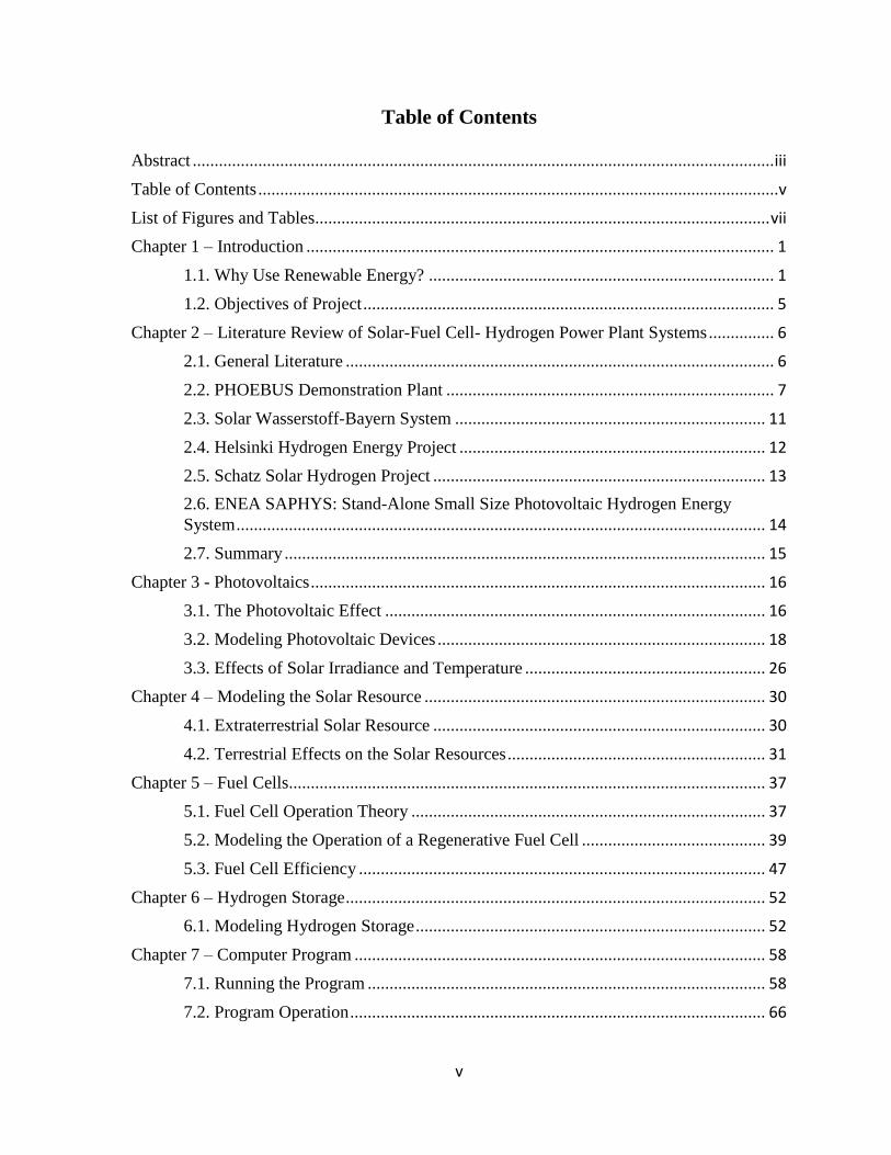
(3.1)

19

where

= light generated current (A),

= diode current (A) and

= shunt current (A).

The diode current can be represented by:

(3.2)

where

= reverse saturation current (A),

q = charge of an electron, 1.602x10-19

coulombs,

V = operating voltage of the cell (V),

I = operating current of the cell (A),

= series resistance (ohms),

k = Boltzmann constant, 1.381x10-23

J/K,

T = operating temperature of the cell (K) and

= completion factor, (ideality factor, m (m=1 if ideal), times the number of cells in

series, Ns.

and the shunt current is represented by:

(3.3)

where

= shunt resistance

Substitution of Eqns. 3.2 and 3.3 into 3.1 yields the overall I-V characteristic equation needed

to model the equivalent circuit shown in Figure 3.2,

. (3.4)

20

In order to solve this equation at any operating temperature or solar irradiance, the following

five values must be determined: , , , and . This can be accomplished by using

common solar module parameters that most manufacturers provide in their documentation.

These are , , , , and which represent: short circuit

current, open circuit voltage, current at maximum power, voltage at maximum power,

temperature coefficient for open circuit voltage, and temperature coefficient for short circuit

current, respectively. These values are given at reference conditions, usually 1000 W/m2

and

298 K. In order to use these values, Eqn. 3.4 can be solved at four different operating points

in order to generate four independent versions of this equation. These points are the open

circuit voltage, short circuit current, maximum power point, and an off reference condition

point. Solving for this system of nonlinear equations can be done numerically using many

different techniques.

For long-term modeling work, it is essential that I-V curves describing module performance

at any operating condition be generated in a timely manner with a high probability of

converging on the correct solutions. Because this set of equations is highly nonlinear and

very sensitive to initial guesses, it is not suitable for long-term modeling work which may

require tens of thousands of hourly calculations. The probability of failing to converge is too

great. As such, some assumptions can be made in order to simplify the I-V equation shown in

Eqn. 3.4 in order to make it suitable for long-term modeling calculations. Much of the

following manipulations and assumptions were derived by Townsend (1989) which allows

for , , and to be solved for directly.

By assuming that the shunt resistance is infinite, it is possible to neglect the shunt current

which removes the third term in Eqn. 3.4. This assumption is justifiable because the shunt

resistance is usually much larger than the other resistances within a PV cell and because the

shunt resistance only plays a large role when solar irradiance is low. Townsend (1989) found

that for a typical module receiving 1030 W/m2

of solar energy, assuming an infinite shunt

resistance only introduced an error in the maximum power of about 0.6% as compared to the

same module with a shunt resistance of 500 ohms. In low light conditions of 125 W/m2, the

21

error introduced in the maximum power is about 4.5%. This assumption is justified on the

grounds that the introduced error is relatively small for normal irradiances and that by

making this assumption, the robustness of the long-term model is greatly increased. The

equivalent circuit is shown in Figure 3.3.

Figure 3.3: Equivalent circuit of a PV cell with an infinite shunt resistance

Applying this assumption, Eqn. 3.1 becomes

(3.5)

and the I-V equation simplifies to

. (3.6)

When the shunt resistance is assumed to be infinite, one less variable (and one less equation)

is needed to solve for the necessary parameters: , , and . By solving Eqn. 3.6 at the

following three points: short circuit current, open circuit voltage and the maximum power

point, three equations are generated. Eqn. 3.6, solved at the short circuit current, I=ISC and

V=0, is

. (3.7)

The second equation that can be generated at the open circuit voltage is

22

(3.8)

where I=0 and V=VOC.

The third independent equation, solved at the maximum power point is

(3.9)

where I=IMP and V=VMP.

Eqn. 3.6 can be substituted into the equation for electrical power, P=IV, giving

. (3.10)

The next step is to take the derivative of this equation with respect to voltage and set it equal

to zero.

(3.11)

Taking these derivatives and replacing V with VMP and I with IMP produces a fourth

independent equation,

. (3.12)

These four equations (Eqns. 3.7, 3.8, 3.9, 3.12) can be solved using the Newton-Raphson

method, but are still quite unstable when poor initial guesses are made. By omitting some of

the smaller terms, these equations can be simplified further so that an explicit solution can be

23

found using successive substitutions or simpler solving routines. The additional

simplifications are as follows:

1) In Eqn. 3.8, the „-1‟ that is subtracted from the exponential term can be

dropped. This is because at the open circuit voltage point the value within the

exponential is on the order of 105. By dropping the „-1‟, no significant error is

introduced. The „-1‟ can also be dropped from Eqn. 3.9 and Eqn. 3.6 for cases

where Eqn. 3.6 is used at larger voltages.

2) Assume that IL is equivalent to ISC. While these values differ in practice, they

are usually similar to several significant digits. This assumption introduces

minimal error and helps to allow for a direct solve instead of more complex

solving routines that may regularly fail to converge.

With these simplifying assumptions, Eqns. 3.7, 3.8 and 3.9 become the following three

equations, respectively:

, (3.13)

(3.14)

and

. (3.15)

From here, Eqn. 3.14 can be solved for Io and substituted into Eqns. 3.6 (neglecting the „-1‟

term as mentioned above) and 3.15. Doing so yields the following equation,

(3.16)

and the equation for the current at the maximum power point becomes

(3.17)

24

The next step is to derive another independent equation in a manner similar to how Eqn. 3.12

was derived, except using the new I-V equation (Eqn. 3.16) for the derivative calculations.

After doing so, the equation for the derivative at the maximum power point is

(3.18)

Solving Eqn. 3.17 for Rs and substituting it into Eqn. 3.18 leaves a simple equation that can

be used to solve for ,

. (3.19)

From, here Rs and Io can be found using the following two equations:

(3.20)

and

. (3.21)

By using the previous equations, the values of , , and can be determined at the

reference conditions. and , however, vary with the operating conditions. is dependent

on both the temperature and solar irradiance while only varies with temperature. and

are both irradiance and temperature independent. Off reference values of can be calculated

from

(3.22)

where

S = solar irradiance at the operating value (W/m2)

= solar irradiance at the reference conditions (usually 1,000 W/m2)

= temperature coefficient for the open circuit voltage, often supplied by the

manufacturer (A/K)

25

The value of , when the solar module is operating at non-reference conditions, can be found

from

(3.23)

where

= reverse saturation current at the reference conditions

= band gap energy for the semiconductor material at the reference temperature

(for silicon this value is 1.12 eV at 298 K)

= band gap energy at the operating temperature

The band gap energy varies with temperature and can be calculated using

(3.24)

where

C = 2.677x104

eV/K for silicon

Once the values for , , and are determined at the operating conditions of the solar

module (irradiance and temperature), the following simplified I-V equation (modified from

Eqn. 3.6) can be solved for I and V over the operating range of the module,

. (3.25)

There are many ways this can be accomplished but the method used in this research was to

find the open circuit voltage at the operating conditions by solving Eqn. 3.8 for VOC and then

dividing this value into steps of 100. From here these stepwise values of voltages are then

substituted into Eqn. 3.25 and a solver routine is used to determine the corresponding values

of current, I. After doing so, I-V characteristic curve shown in Figure 3.4 can be generated.

26

Figure 3.4: Operating curves for a PV module showing current vs. voltage (I-V) and

power vs. voltage (I-P).

The power curve for this module can be found using the relationship P=IV. As can been

seen, the operating point for maximum power is located at a voltage that corresponds to the

“knee” of the I-V curve. The resistance of the load determines the operating point on the I-V

curve, but devices such as maximum power point trackers (MPPT) can be utilized in order to

force the module to operate at the maximum power point with the MPPT operating with an

efficiency of around 95%.

3.3. Effects of Solar Irradiance and Temperature

The effects of solar irradiance and cell temperature play a large role in the I-V curve for any

PV module. Figure 3.5 shows the effects of varying solar irradiance on the operating curve.

Different values for solar irradiance effectively shift the curve upwards or downwards. The

higher the irradiance, the more the curve is shifted upwards, leading to higher power outputs

from the PV module.

27

Figure 3.5: Effects of solar irradiance (S) on the I-V curve of a typical PV module

where T=298K.

Figure 3.6: Effects of temperature on the I-V curve of a typical module with

S=1000W/m2.

28

Figure 3.6 shows the effects of temperature on the I-V curve of a typical PV module.

Different cell temperature values move the I-V curve left or right with lower temperatures

shifting the curve right, leading to higher power outputs. Thus, it is essential to operate most

PV devices at the lowest temperatures possible to maximize power output. Techniques to

accomplish this can range from active cooling systems to simple solutions such as leaving an

air gap when roof-mounting panels to allow for higher convection heat transfer.

An equation that relates the back surface module temperature of a PV module to the wind

speed and solar irradiance is given by King et al. (2003),

(3.26)

where

= back surface module temperature (C),

= wind speed (m/s) and

= ambient air temperature.

Both the wind speed and the ambient air temperature are included in hourly TMY3 data. The

coefficients for a and b are empirically derived coefficients that account for the upper limit in

module temperature at low wind speeds and high solar irradiance and the rate of change in

module temperature as wind speed decreases, respectively. It is important to note that Eqn.

3.26 calculates the back surface temperature of the module, but it is the cell temperature that

should be used for the temperature values in the PV equations. Once the back surface

temperature is determined, the cell temperature can be calculated by:

(3.27)

where

= temperature difference between the cell and the back surface of the module at

1000 W/m2.

29

The values for a, b and are dependent on the mounting type that is chosen. Empirically

derived values are given in Table 3.1.

Table 3.1: Empirical coefficients for use in Eqns. 3.26 and 3.27 [King et al. (2003)].

Mounting Type a b (C)

Open rack -3.47 -0.0594 3

Close roof mount -2.98 -0.0471 1

Chapter 3 was concerned with how to derive the operating curve for a PV module and how to

calculate and take into account the solar irradiance, cell temperature and wind speed. This

chapter provides the necessary tools to determine the power curve for a PV module at any

operating condition. Once the power output of the solar array is known, it can be sent to the

regenerative fuel cell to electrolyze water into hydrogen and oxygen.

30

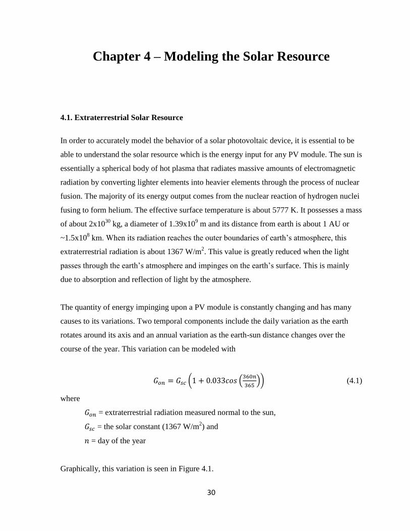
Chapter 4 – Modeling the Solar Resource 4.1. Extraterrestrial Solar Resource

In order to accurately model the behavior of a solar photovoltaic device, it is essential to be

able to understand the solar resource which is the energy input for any PV module. The sun is

essentially a spherical body of hot plasma that radiates massive amounts of electromagnetic

radiation by converting lighter elements into heavier elements through the process of nuclear

fusion. The majority of its energy output comes from the nuclear reaction of hydrogen nuclei

fusing to form helium. The effective surface temperature is about 5777 K. It possesses a mass

of about 2x1030

kg, a diameter of 1.39x109 m and its distance from earth is about 1 AU or

~1.5x108 km. When its radiation reaches the outer boundaries of earth‟s atmosphere, this

extraterrestrial radiation is about 1367 W/m2. This value is greatly reduced when the light

passes through the earth‟s atmosphere and impinges on the earth‟s surface. This is mainly

due to absorption and reflection of light by the atmosphere.

The quantity of energy impinging upon a PV module is constantly changing and has many

causes to its variations. Two temporal components include the daily variation as the earth

rotates around its axis and an annual variation as the earth-sun distance changes over the

course of the year. This variation can be modeled with

(4.1)

where

= extraterrestrial radiation measured normal to the sun,

= the solar constant (1367 W/m2) and

= day of the year

Graphically, this variation is seen in Figure 4.1.

31

Figure 4.1: Variation in extraterrestrial solar radiation with the day of the year.

4.2. Terrestrial Effects on the Solar Resources

Because of the effects of earth‟s atmosphere, the solar radiation falling on a module is

commonly divided into two general components; these are the direct and diffuse components.

Direct radiation, or sometimes called beam radiation, is the amount of solar radiation that

directly impinges upon a module, while diffuse radiation refers to radiation that is scattered

by the atmosphere and then reaches the module. There are several manners in which to

envision and calculate the diffuse component of solar radiation. One method is to consider

the sky to be isotropic which implies the scattered radiation is uniform in all directions.

While considering the sky to be isotropic is simple to understand and allows for simplistic

calculations, a more advanced manner to envision diffuse radiation is to consider circumsolar

scattered radiation and a scattered component from the horizon in addition to the isotropic

scattered radiation from the sky; this is an anisotropic sky model. This treatment of the

diffuse radiation is used in this work utilizing a model developed by Perez et al. (1988).

The total solar radiation impinging on a horizontal surface located on the surface of the earth

is the sum of the beam and diffuse components,

(4.2)

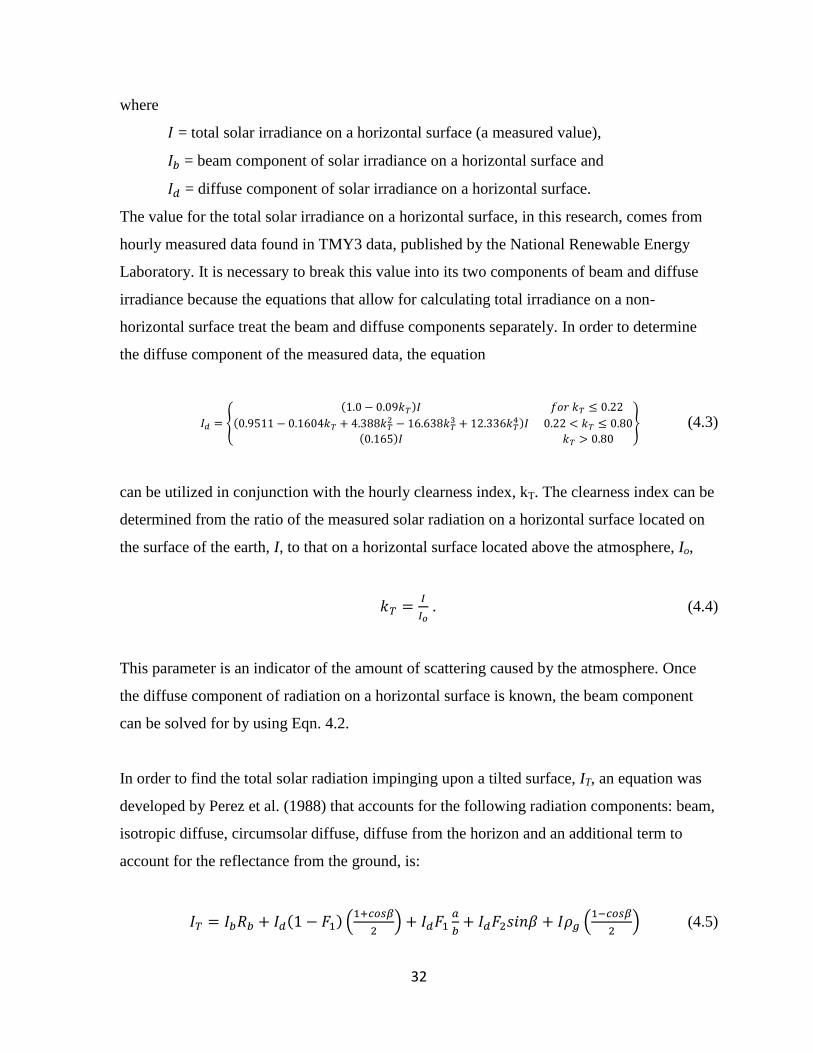
32

where

= total solar irradiance on a horizontal surface (a measured value),

= beam component of solar irradiance on a horizontal surface and

= diffuse component of solar irradiance on a horizontal surface.

The value for the total solar irradiance on a horizontal surface, in this research, comes from

hourly measured data found in TMY3 data, published by the National Renewable Energy

Laboratory. It is necessary to break this value into its two components of beam and diffuse

irradiance because the equations that allow for calculating total irradiance on a non-

horizontal surface treat the beam and diffuse components separately. In order to determine

the diffuse component of the measured data, the equation

(4.3)

can be utilized in conjunction with the hourly clearness index, kT. The clearness index can be

determined from the ratio of the measured solar radiation on a horizontal surface located on

the surface of the earth, I, to that on a horizontal surface located above the atmosphere, Io,

. (4.4)

This parameter is an indicator of the amount of scattering caused by the atmosphere. Once

the diffuse component of radiation on a horizontal surface is known, the beam component

can be solved for by using Eqn. 4.2.

In order to find the total solar radiation impinging upon a tilted surface, IT, an equation was

developed by Perez et al. (1988) that accounts for the following radiation components: beam,

isotropic diffuse, circumsolar diffuse, diffuse from the horizon and an additional term to

account for the reflectance from the ground, is:

(4.5)

33

where

= ratio of beam radiation on a tilted surface to that of the horizontal surface

= circumsolar and horizon brightness coefficients

= slope of the solar module

= constants to account for the angles of incidence of the cone of circumsolar

radiation

= ground reflectance

Numerous additional equations are required to solve Eqn. 4.5. The ratio of beam radiation on

a tilted surface to the horizontal surface, Rb, is an essential parameter for determining the

total amount of beam radiation impinging on the module. Near sunset and sunrise, Rb,

changes very rapidly and becomes too large which causes poor results. In order to avoid this

problem, it is best to average the values for Rb over the hour:

(4.6)

where

= angle of incidence of the beam radiation on the tilted module‟s surface

= zenith angle, or the angle of incidence of the beam radiation on a horizontal

surface

= hour angle, or angular displacement of the sun east or west of the meridian.

changes by 15˚ per hour. Morning and evening values are negative and positive

respectively.

Eqn. 4.6 can be integrated in terms of the declination, latitude, module tilt, module azimuth

angle and hour angle giving

(4.7)

where

34

(4.8)

and

(4.9)

and the utilized angles are

= declination, or angular position of the sun at solar noon, -23.45˚ ≤ 23.45,

= latitude of the solar module, -90˚ ≤ ϕ 90˚,

= the direction of the module‟s normal vector in relation to the local meridian,

180˚ ≤ γ 180˚ where γ = 0 when the module is pointing due south and

= slope of the module from a horizontal surface.

The angle of incidence, θ, can be found from,

.

. (4.10)

Once Rb is known, the values for F1 and F2 can be calculated. These coefficients are required

in order to determine the three diffuse components of the solar radiation scattered by the

atmosphere. The equations providing F1 and F2 are

(4.11)

and

(4.12)

where

= brightness coefficient that incorporates air mass and

= coefficients that have been statistically derived by Perez et al. (1987)

35

The brightness coefficient, , can be found with

. (4.13)

In this equation m is the air mass, which is the ratio of the mass of atmosphere that a beam of

light passes through compared to the mass of atmosphere that the beam would pass through if

the sun were directly overhead. For angles less than 70˚, m=1/cos . When the sun is nearer

the horizon, the denominator approaches zero which causes m to be inaccurately high. For

higher angles, an alternative equation, developed by Kasten and Young (1989) is more

accurate,

θ θ (4.14)

where is in degrees. This equation is valid for all zenith angle values.

The f coefficients in Eqns. 4.11 and 4.12 can be found using Table 4.1 after determining the

value of ε,

θ

θ (4.15)

where is in degrees. Once ε is determined, Table 4.1 can be used to determine the values

of f11, f12, f13, f21, f22 and f23.

After these values are determined, terms 1, 2, 4 and 5 on the right-hand side of Eqn. 4.5 can

be calculated. Term 3 contains two parameters, a and b, which account for the angles of

incidence of the cone of circumsolar radiation. Both a and b can be determined with

(4.16)

and (4.17)

36

Substituting all of the previously calculated values into Eqn. 4.5 yields the final value of

solar irradiance on a tilted surface, . This is the value that gets plugged into Eqn. 3.22 for S

in order to solve for the light-generated current at non-reference values of solar irradiance.

Losses from the solar radiation passing through the module‟s glass are assumed here to be

negligible.

Table 4.1: Brightness coefficients from Perez et al. (1988).

Range of f11 f12 f13 f21 f22 f23

0-1.065 -0.196 1.084 -0.006 -0.114 0.180 -0.019

0.065-1.230 0.236 0.519 -0.180 -0.011 0.020 -0.038

1.230-1.500 0.454 0.321 -0.255 0.072 -0.098 -0.046

1.500-1.950 0.866 -0.381 -0.375 0.203 -0.403 -0.049

1.950-2.800 1.026 -0.711 -0.426 0.273 -0.602 -0.061

2.800-4.500 0.978 -0.986 -0.350 0.280 -0.915 -0.024

4.500-6.200 0.748 -0.913 -0.236 0.173 -1.045 0.065

6.200 + 0.318 -0.757 0.103 0.062 -1.698 0.236

37

Chapter 5 – Fuel Cells 5.1. Fuel Cell Operation Theory

Fuel cells are devices that convert chemical energy into electrical energy in a one-step

conversion process without the use of moving parts. In any chemical reaction, two or more

chemical species change the way that they are bonded to each other. Bonds are facilitated by

electrons, and creating or breaking bonds results in the release or absorption of energy by the

species involved. Fuel cells work by spatially separating a single chemical reaction into two

half-reactions that occur at an anode and a cathode, which are separated by an electrolyte. A

common chemical reaction that fuel cells utilize is that of hydrogen and oxygen reacting to

form water. In a proton exchange membrane fuel cell (PEMFC), diatomic hydrogen splits

into hydrogen ions (protons) and electrons on the surface of the anode, supported by a

catalyst material such as platinum. Both the ions and electrons then travel towards the

cathode by taking two separate paths, where they meet up at the cathode, react with oxygen

and form water. The load that is to be powered is placed between the anode and cathode,

connected by an external electric circuit, where the flow of electrons (current) can power the

load. The hydrogen ions (protons) traverse across the electrolyte to reach the cathode.

In order to store the electric energy from the PV array as hydrogen, a regenerative fuel cell

system can be used to convert water into hydrogen and oxygen and vice versa. This process

requires an electric input as it is not a spontaneous process. The reverse process requires

hydrogen and oxygen and produces water, electricity and heat. By using this reversible

process to generate and consume hydrogen, electricity can be produced 24 hours a day to

match any demand, given the right choice of system component sizes.

There are many different types of fuel cells which differ in their materials, construction,

charge carrier species, catalyst material and electrolyte. The following table gives brief

details of some of the more common fuel cell types.

38

Table 5.1: Some common fuel cell type specifications [Fuel Cell Fundamentals (2009)].

Fuel Cell Type Electrolyte Charge

carrier

Fuel

choices

Operating

temperature

Solid oxide Ceramic (Yttria-stabilized

zirconium)

O2-

H2, CH4,

CO

600-1000˚C

Polymer electrolyte

membrane

Carbon based polymer

(Nafion®)

H+ H2,

methanol

80˚C

Phosphoric acid Liquid H3PO4 H+ H2 200˚C

Alkaline Liquid KOH OH- H2 60-220˚C

Molten carbonate Molten

H2, CH4 650˚C

In this research, a regenerative solid oxide fuel cell (SOFC) was selected for several reasons.

SOFCs, due to their high temperatures, can realize higher efficiencies and produce good

quality waste heat compared to other types of fuel cells. The electrical efficiency can be

around 50-60%, and if cogeneration is used, efficiencies of around 90% can be realized.

SOFCs are usually operated between 600 ˚C and 1000 ˚C; because of this, expensive

catalysts such as platinum are not required, which allows for lower material costs.

Furthermore, because of the high temperatures, a variety of fuels can directly be used such as

hydrogen, methane and carbon monoxide. An external fuel reformer is not required as the

high temperatures allow for internal reforming. Solid oxide fuel cells are not without their

problems, however. Their operating temperature rules out several material choices. Ceramics

are often used for this reason. During start up and shut down, thermal stresses can cause

material failure or sealing issues if they are not properly designed.

A SOFC uses the following reaction to generate electricity, water and heat,

. (5.1)

When a SOFC is operated in the reverse direction (electrolysis mode), water is split into

hydrogen and oxygen. This process is not spontaneous, so energy must constantly be added

to encourage the reaction to proceed,

. (5.2)

39

During fuel cell mode operation, hydrogen and oxygen flow across the anode and cathode,

respectively. A reaction takes place on the surface of both electrodes simultaneously, which

is promoted by the catalyst. At the cathode, the following reaction occurs,

. (5.3)

The electrons that are supplied to the reaction above are produced at the anode and

transferred to the cathode by means of the external electric circuit. Once oxygen is split into

oxygen ions at the cathode, these ions diffuse across the ceramic electrolyte layer where they

meet with hydrogen to form water. This reaction is

. (5.4)

In electrolysis mode, these reactions happen in reverse.

5.2. Modeling the Operation of a Regenerative Fuel Cell

In this research a 1-D fuel cell model is used to predict the performance of a regenerative

solid oxide fuel cell over time. This model is based off existing models as found in the

literature [Kim et al. (1999) and Chan et al. (2001)] with some simplifications given by

O‟Hayre (2009). In a solid oxide fuel cell, all of the reactants and products exist in the gas

phase, which makes modeling much easier than other fuel cell types such as PEM fuel cells

where the reactants and products exist in the liquid form and water can diffuse across the

membrane with the protons. Other factors in SOFC‟s can complicate modeling such as

nonisothermal behavior and thermal expansion-stresses, but by making a few simple

assumptions and focusing only on species concentration profiles, the model can be reduced to

a relatively simple, yet fairly accurate, form for use in long term modeling.

40

In order to generate a plot of current density vs. voltage, a flux balance is carried out on the

species entering and leaving the SOFC. Nitrogen (which composes almost 79% of the

entering reactant stream at the cathode) is neglected as it does not participate in the fuel cell

reactions. Each of these fluxes can be directly related to the current density of the cell.

Figure 5.1: Diagram of a SOFC and its chemical species flows.

By carefully analyzing the chemical species entering, leaving and going through the fuel cell,

the current density of the cell can be calculated. By examination, it can be seen that

(5.5)

It can be said, then, that the current density is equal to the twice oxygen ion flux across the

electrolyte. This is also equal to the net hydrogen flux into the anode and the net oxygen flux

into the cathode. Mathematically, this flux balance can be represented by

(5.6)

41

where

j = current density (A/cm2),

F = Faraday‟s constant (96485 C/mol),

= oxygen ion flux across the electrolyte membrane,

= net hydrogen flux into the anode and

= net oxygen flux into the cathode.

By using Eqn. 5.6 and solving the 1-D model‟s equations in terms of current density, j,

information pertaining to the chemical species‟ concentrations within the fuel cell can be

used to derive the activation and ohmic overvoltages. Before going any further, it is essential

to identify the simplifying assumptions that are used in this 1-D model.

1) Convective transport within the fuel cell is ignored. Obtaining accurate values

for convection is often very difficult to accomplish and since convective

transport is typically in the y-direction in Figure 5.1 and the 1-D model

considers only transport in the z-direction, it is neglected.

2) Diffusive transport in the flow channels is neglected, but not in the electrodes.

Diffusion in the flow channels is much more trivial than convective transport

and since convective transport is ignored, diffusion can be as well.

3) All ohmic losses derive from the electrolyte. This is a reasonable assumption

for most fuel cell types as ohmic losses in the electrolyte from ionic

conduction are generally far greater than other ohmic losses.

4) Reaction kinetics at the anode are neglected. The activation losses at the

cathode are usually much larger than at the anode because oxygen reduction is

the more sluggish process.

5) The catalyst layers are assumed to be extremely thin so that they can be

assumed to have no thickness. Although in a SOFC, the catalyst layer and

electrode comprise a single body of definite thickness, most of the reactions

are localized to a thin region between the electrodes/catalysts and the

electrolyte, so this assumption is still valid.

6) Water exists only as vapor. Since a SOFC operates at temperatures hundreds

of degrees above the boiling point of water, this is a justified assumption.

42

7) The SOFC is cathode or electrolyte supported. Because the ceramic materials

in SOFCs can be especially brittle, it is common to thicken one of the cell

components (anode, electrolyte or cathode) to support the fuel cell structure.

Here, the SOFC cannot be anode supported if the above assumptions are to be

used such as neglecting the anode reaction kinetics.

From these assumptions, governing equations can be developed which determine how the

concentrations of the chemical species vary throughout the fuel cell. By calculating these

concentrations (as a function of current density), the mass transport overvoltage, ηconc,

activation overvoltage, ηact, and ohmic overvoltage, ηohmic, can be calculated. Once these are

known, the operating voltage of the cell can be determined at any current density by:

(5.7)

where

= thermodynamically predicted reversible fuel cell voltage (V).

In order to obtain the governing equations needed to solve Eqn. 5.7, the processes occurring

at the electrode layer, electrolyte and catalyst must be considered. At the electrode layer, the

diffusion of the chemical species, H2, O2, and H2O can be modeled by using Fick‟s law of

diffusion,

(5.8)

where

= diffusion flux of species i (mol/m2s),

= effective diffusivity of species i within the catalyst layer (m2/s),

= concentration of species i in the catalyst layer (mol/m

3),

= concentration of species i in the flow channel (mol/m

3) and

= electrode thickness (m).

By the ideal gas law (pi=ciRT) and the equation for partial pressure (pi=pxi), Eqn. 5.8 can be

rewritten in the terms of total pressure and the mole fraction of species i,

43

(5.9)

where

P = total pressure at the electrode,

= mole fraction of species i, and

= length along the z-axis.

At the electrolyte layer, the oxygen ion flux is proportional to the current density as per Eqn.

5.6,

(5.10)

and the total ohmic voltage loss is simply

(5.11)

where

= area specific resistance (Ωcm2), the product of the area and resistance of

the cell,

= thickness of the electrolyte (cm) and

= electrolyte conductivity (1/Ω).

The conductivity of the electrolyte can be found from

(5.12)

with the variables, ASOFC and ΔGact being derived experimentally.

The total ohmic resistance is equivalent to

. (5.13).

44

In the catalyst layer, it was assumed that only cathode reaction kinetics exist and the anode

reaction kinetics are negligible. The cathodic overvoltage is thus largely dependent on the

partial pressure of oxygen and a simplified form of the Butler-Volmer equation can be used,

assuming an ideal gas,

(5.14)

where

= charge transfer coefficient,

= exchange current density (A/cm2),

= total pressure at the cathode and

= mole fraction of oxygen at the catalyst layer.

Because Eqn. 5.13 accounts for the oxygen concentration, both the activation losses, ηact, and

the concentration losses, ηconc, are accounted for by solving for the cathodic overvoltage.

In determining the cathodic overvoltage, the mole fraction of oxygen in the catalyst layer

cannot be easily measured. What is known, however, is the oxygen mole fraction at the

oxygen inlet. This value is about 21% since air is what is supplied on the cathode side. In

order to solve for the mole fraction in the catalyst layer, Eqn. 5.9 can be integrated with the

boundary condition of 21% at the flow channel inlet. Doing so yields

. (5.15)

Substituting Eqn. 5.15 into 5.14 generates the following relationship which can be used to

calculate the cathodic overvoltage at any current density.

. (5.16)

45

Now that the mass transport overvoltage, activation overvoltage and ohmic overvoltage have

been calculated, Eqns. 5.13 and 5.16 can be substituted into Eqn. 5.7 to yield the final

equation needed to calculate the operating voltage of a SOFC given the current density

. (5.17)

The reversible cell voltage can be calculated using

(5.18)

where

= standard state reversible fuel cell voltage (V),

= change in entropy with operating temperature (kJ/mol),

= standard state temperature (generally 298 K),

= operating temperature of the fuel cell (K),

= mole fraction of hydrogen and

= mole fraction of oxygen.

To generate a j-V plot by using Eqn. 5.17, the current density can be iterated and solved for

V. This plot is shown in Figure 5.2. The output power is also shown which was generated

using P=jV and plotted against the current density. It should be noted that the maximum

power point is not at the highest current density. In practice, a fuel cell should be operated on

the left side of the peak on the power curve. Operating on the right side uses more fuel but

does not produce any more power than can be obtained by operating on the left side of the

curve.

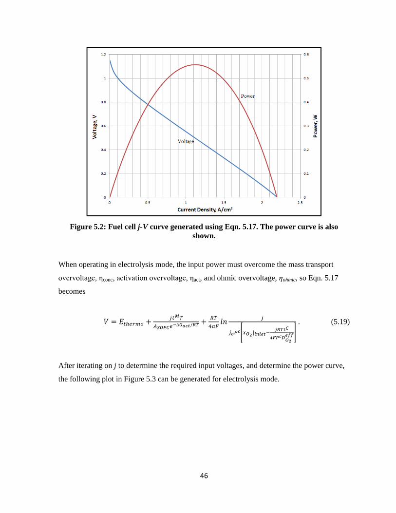
46

Figure 5.2: Fuel cell j-V curve generated using Eqn. 5.17. The power curve is also

shown.

When operating in electrolysis mode, the input power must overcome the mass transport

overvoltage, ηconc, activation overvoltage, ηact, and ohmic overvoltage, ηohmic, so Eqn. 5.17

becomes

. (5.19)

After iterating on j to determine the required input voltages, and determine the power curve,

the following plot in Figure 5.3 can be generated for electrolysis mode.

47

Figure 5.3: Electrolysis mode j-V curve generated using Eqn. 5.19. The power curve is

also shown.

5.3. Fuel Cell Efficiency

When a fuel cell is in operation, hydrogen fuel is consumed at a rate that is proportional to

the current through the cell. Some of the fuel may pass through the cell without reacting or

participate in side reactions that produce no power, however. For these reasons, fuel cells

have a value known as a fuel utilization efficiency, εfuel,

(5.20)

where

= fuel supply rate (mol/s),

= current through the cell (A) and

= molar quantity of electrons produced per mole of fuel reacted (For H2, n=2).

If more fuel is supplied than is consumed by the cell, some will be wasted if it is not

recycled. This is reflected in the fuel utilization efficiency. There are typically two manners

48

in which to supply a fuel cell with fuel. The first method is to supply a constant flow rate,

perhaps at a rate that is enough to prevent the cell from starving at the maximum current

density. This method, however, results in much of the fuel being wasted. This is especially

true at low current densities. A more practical approach is to use a constant stoichiometry

flow method. The fuel flow rate into the cell is constantly adjusted so that the cell receives a

small amount more than what is actually required in order to prevent starvation. This method

can be much more efficient than a constant fuel flow rate; less is wasted. If an operating fuel

cell requires 10 mol/s of fuel and 12 mol/s of fuel is supplied, the fuel cell is operating at 1.2

times stoichiometric. The stoichiometric factor, λ, is given by

. (5.21)

The fuel utilization efficiency is thus

. (5.22)

In this research, the excess hydrogen leaving the fuel cell was considered to be recycled and

set to 1. In order to determine the overall efficiency of a fuel cell in operation, two other

terms must be specified: the reversible thermodynamic efficiency, εthermo, and the voltage

efficiency, εvoltage. The reversible thermodynamic efficiency arises because only part of the

enthalpy contained within a fuel is converted into useful work and the voltage efficiency is

due to the fact that there are irreversible kinetic losses with the fuel cell. These two

efficiencies are given by

(5.23)

and

(5.24)

where

= operating voltage of the fuel cell (V) and

= thermodynamically predicted reversible voltage (V)

49

Putting Eqns. 5.21, 5.22, 5.23 and 5.24 together yields the overall fuel cell efficiency which

is a function of the current density, operating voltage and indirectly other parameters such as

temperature and pressure,

. (5.25)

A visual representation of how the total fuel cell efficiency varies over the operating range of

current densities, using both constant stoichiometry and constant fuel flow rate conditions, is

shown in Figure 5.4. As can be seen, with a constant stoichiometry flow method, a fuel cell

realizes the highest efficiencies at the lowest current densities.


conditions. For constant stoichiometry =1 and for constant flow rate, 1.1 times the

required flow rate at maximum current is supplied.

50

As a fuel cell converts the chemical potential energy stored within a fuel into electrical

energy, some amount of heat is always produced as a byproduct of the reaction. This is

mainly due to the reconfiguration of the chemical bonds of the reactants and can be

calculated by considering the change in enthalpies between the products and reactants. This

enthalpy change, also called the heat of combustion, can be calculated by using Eqn. 5.25 for

the hydrogen-oxygen reaction that takes place within the fuel cell.

(5.26)

where h represents the enthalpies of water, hydrogen and oxygen. The one half is due to the

stoichiometry of Eqn. 5.1.

For a fuel cell operating at 1000 K, the heat of reaction is -247.865 kJ/mol. The negative sign

indicates that this reaction releases energy. Since this value reflects the total amount of

energy released by this chemical reaction, it can be determined how much of it is given off as

heat by determining how much fuel is being consumed and how much electrical energy is

produced. From the following relationship, the amount of heat produced by a fuel cell can be

determined,

Etotal n hreaction Eheat Eelectricity (5.27)

where n is the number of moles of fuel consumed. Rearranging this equation and solving for

gives the amount of heat released over a given time frame,

Eheat Eelectricity n hreaction . (5.28)

The operating point of the fuel cell can be calculated using Eqn. 5.17 to determine the current

and voltage through the cell (while taking into account the number of cells in series or

parallel). Multiplying these two values together gives the electrical power out of the fuel cell.

From Eqn. 5.21, the molar rate at which hydrogen is being consumed can be determined.

51

Multiplying the power and the rate of hydrogen consumption by the time over which the

reaction occurs gives the total energy released by the reaction.

In order to determine the heat flows when the fuel cell is in electrolysis mode, the situation is

only slightly more complex. For an electrolyzer the amount of heat produced (or consumed)

is dependent on the operating voltage. At standard temperature and pressure, the amount of

heat exchanged with the environment is

(5.29)

where

= operating voltage of the electrolyzer (V) and

= current through the electrolyzer (A)

The „1.484‟ term is the hypothetical voltage that could be attained if all of the enthalpy

contained within the fuel were converted to electricity.

The value for Q can be negative or positive depending on the operating point of the cell. If it

is negative, the reaction is endothermic so heat must be applied to the cell to prevent the

temperature from dropping. In order to determine how much heat must be supplied or

removed from the electrolyzer, Eqn. 5.28 can be used again; but in order to calculate the

amount of electrical energy forced through the cell, the operating point is determined by Eqn.

5.19. Once again, taking into account the time over which the reaction occurs, the total

amount of heat energy released or consumed can be determined. The sign of in Eqn.

5.28 will indicate if heat must be added or removed.

52

Chapter 6 – Hydrogen Storage

6.1. Modeling Hydrogen Storage

Hydrogen is the lightest and most abundant element in the universe. Unfortunately on Earth,

it is not found in its pure form but is chemically bonded to other elements like oxygen in the

case of water. Energy must be expended in order to extract hydrogen. As such it is not a

source of energy, but an energy carrier. It shows promise as a fuel for transportation purposes

for land and air vehicles owing to its high gravimetric energy density. By mass it has about

three times as much energy as gasoline. The gravimetric energy content of hydrogen is about

123 MJ/kg or 34.2 kWh/kg.

Hydrogen can be used to power land and sea vehicles with great efficiency if fuel cells are

utilized. Hydrogen has also been used as a rocket propellant with great success; the second

and third stages of the Saturn V rocket used liquid hydrogen to take humans to the Moon.

Hydrogen powered fuel cells have also been used in space missions to generate electricity,

heat and drinking water for the astronauts. It is also receiving great interest as a potential fuel

for industrial and domestic electricity and heat generation.

Some of hydrogen‟s key advantages are that it is non-toxic and clean burning, producing

only water vapor as a product of combustion; it does not produce greenhouse gases. It is also

a renewable form of energy. After being reacted with oxygen to generate water and release

energy, the water can then be converted back to hydrogen using any of several different

processes. Some of these processes include chemical, electrolytic, thermolytic, photolytic or

biological pathways. In this research, electrolytic hydrogen production is utilized with a

regenerative solid oxide fuel cell whose operation was outlined in Chapter 5.

53

Hydrogen is generated by the solar-hydrogen plant when electrical energy from the PV array

is forced through the regenerative fuel cell in electrolyzer mode. The current through the cell

is directly proportional the hydrogen generation rate,

. (6.1)

As hydrogen is produced, it must be stored in some form or another. One of hydrogen‟s main

drawbacks is its low volumetric energy density. For example, comparing hydrogen to

methane at atmospheric pressure, hydrogen has about one third the combustion energy as

methane. Even in its liquid form, which requires cooling to around 20 K, hydrogen has a

lower volumetric energy density than gasoline. Compressed to 700 bar, the volumetric

energy density of gaseous hydrogen is 5.6 MJ/L or 1.6 kWh/L whereas one liter of gasoline

contains about 36 MJ or 10 kWh. Because of this low volumetric energy density, most

hydrogen storage systems tend to be bulky and heavy.

There are many ways to store hydrogen depending on the application. The simplest way to

store hydrogen is by compressing it into a rigid container. If space requirements exist for a

certain application, such as in transportation, then the use of extremely high pressures may be

required. For stationary applications, space requirements are usually not the most important

factor, so lower pressure tanks can be used. Other forms of storage include cryogenic

hydrogen storage which involves cooling hydrogen below its boiling point and storing it in a

chilled, pressure vessel.

Another viable method of storing hydrogen is to use the generated hydrogen to react with

another compound to form a new chemical, ideally one with better storage properties than

pure hydrogen. For example, it can be reacted with CO to produce methane and water. Under

different reaction conditions, the same reactants can form methanol. Both of these chemical

species can hold and store hydrogen more compactly than pure hydrogen can be stored.

Methanol is a liquid at room temperature, for example, so high pressure tanks can be

avoided. Hydrogen can also be reacted with atmospheric nitrogen to generate ammonia

which has been carried out on industrial scales with success.

54

One area of hydrogen storage that is currently receiving great interest is that of metal

hydrides. Metal hydrides are compounds that can form unstable, and hence reversible,

hydride compounds with the addition of hydrogen at high pressure. At low pressures, the

crystalline structure of metal hydrides does not energetically favor the accommodation of

hydrogen into its crystal lattice; but, when the pressure of hydrogen is increased, the

crystalline structure will reorient itself and take in significant amounts of hydrogen.

Theoretically, the volume concentration of metal hydrides can exceed that of liquid

hydrogen. To release hydrogen from the hydride, the temperature must be increased. Because

the reaction kinetics of the hydrides can limit how fast hydrogen can be absorbed or

desorbed, this type of hydrogen storage was not chosen for this research. Compressed

hydrogen storage was selected.

In order to calculate the compression work needed to store gas in a tank, it is important to

first consider the operating pressure of the tank. At lower pressures hydrogen storage can be

modeled using ideal gas law equations. A good cutoff for where the ideal gas laws cannot be

used is around 50 bars as the compressibility factor is just over 1. At 300 bars, the

compressibility factor is about 1.2 [Klell (2010)]. In this case, the use of the ideal gas laws

would predict the mass of hydrogen in a 300 bar vessel to be 20% greater than what it

actually is, as shown in Figure 6.1.

Using the ideal gas law pressure, volume and temperature can all be related by:

(6.2)

where

P = pressure (bars),

V = volume (liters),

n = number of moles of gas,

R = gas constant (8.314x10-2

L-bar/mol-K) and

T = temperature (K).

55

At low temperatures and high pressures, the gas molecules interact with each other much

more, and ideal gas laws cannot be used. In this case, a common approach is to use the Van

der Waals equation,

(6.3)

where a and b are empirically derived constants that depend on the type of gas. For

hydrogen, a = 0.2476 L2bar/mol

2 and b = 0.02661 L/mol [Weast (1972)].

Figure 6.1: Compressibility factors for hydrogen vs. temperature and pressure [Klell

(2010)].

After each hour when the fuel cell is running in electrolyzer mode, an amount of hydrogen is

produced at atmospheric pressure since that is the operating pressure of the fuel cell. This

quantity of gas must then be compressed up to the pressure of the storage tank which varies

each hour. If the tank pressure is low enough, the amount of work required to compress the

newly produced hydrogen can be derived from the ideal gas law and is

56

(6.4)

where

= amount of work required to compress a gas from to ,

= pressure at which hydrogen is produced,

= pressure to which the hydrogen must be compressed.

For non-ideal pressures, a simple relationship like Eqn. 6.4 is not to be found. Instead one

must integrate over the range of pressures using the work equation for compressing a gas.

(6.5)

Both the volume and pressures cannot be determined using the ideal gas law but rather Van

der Waals equation. To solve this numerically, this integral could be broken up into many

steps, solved and summed to yield an accurate work value. This method wasn‟t used in this

work due to long computation times, but we present it here for future developments in the

program. For this reason it was decided to limit the tank storage pressure to 50 bars so that

ideal gas equations could be used. This is not necessarily a poor choice, because even though

low storage pressure results in larger tanks, small tank size need not be an essential parameter

for stationary applications. Furthermore, using smaller pressures results is less energy

required for compression work and hence a more energy efficient system. Throughout this

paper, the storage capacities and tank levels are given in kilograms. As a reference, Figure

6.2 shows the conversion from kilograms to tank volume when pressure is equal to 50 bars.

57

Figure 6.2: Conversion chart between kilograms of hydrogen and volume, given a 50

bar storage tank.

58

Chapter 7 – Computer Program 7.1. Running the Program

The methods and equations developed in the preceding sections were compiled and

organized into a MATLAB program with user-friendly GUIs to simulate long term, steady

state solar-fuel cell-hydrogen electric power plant performance. In order to run a simulation

of the power plant, several parameters need to be specified first, such as the location, demand

data, PV array, regenerative fuel cell, hydrogen storage, simulation run time, etc. In this

section, the reader is walked through the GUI screens in order to demonstrate how to

properly run the program and format the necessary inputs.

To begin, open a new session of MATLAB and point MATLAB to the correct folder that

contains the run files. Begin by running m-file “RunThisOne.m”. The first GUI that opens is

one that specifies if a new simulation is going to be run or if a previously saved simulation is

to be loaded. Figure 7.1 shows this pop-up window. If a previously saved simulation is to be

loaded, it is necessary to have the saved file (MAT-file) in the same folder in which the run

files are located.

For this walkthrough, the “New Simulation” button was selected which immediately brings

up the next GUI allowing the user to specify the location where the solar-fuel cell-hydrogen

power plant will be placed. The two default options are Dayton, OH and Yuma, AZ.

Specifying the location is important because it loads the proper meteorological data and sets

the latitude for calculating the solar resource available to the PV modules. Figure 7.2 shows

this screen.

59

Figure 7.1: Initial GUI upon running the MATLAB code.

Figure 7.2: Location selection GUI.

If desired, the user can also specify another location by using the “Open TMY3 File…”

button. As long as the TMY3 data can be located, any location can be specified for the

program. Typical meteorological year data sets can be found in various places on the internet.

The National Renewable Energy Laboratory website hosts hundreds of these data sets for

various sites throughout the United States. These data sets can be found at the web site:

60

http://rredc.nrel.gov/solar/old_data/nsrdb/1991-2005/tmy3/. If a location other than Dayton

or Yuma is specified, the program will ask the user to input the latitude of the location.

Furthermore, the user should check to make sure the TMY3 data file has the extension

“.xlsx”. If it does not, it should be resaved as such. In this example, Yuma, AZ was selected.

The next GUI that opens allows the user to specify a demand curve. This is the electric

demand that the solar-fuel cell-hydrogen system will try to meet around the clock. Several

default demand curves are given in the listbox in the upper left corner of the screen (see

Figure 7.3). The first four demand curves define a simulated two-story house that was

generated by using the building energy simulation program, eQUEST. These four data sets

are described later in this paper. A constant 2 kW demand load is also found in the list which

can be imagined as a baseload power plant demand curve. Three utility demand loads are

also given for Dayton Power and Light, American Electric Power and the Commonwealth

Edison Company. These last three loads are on the order of gigawatts.

Figure 7.3: Demand load specification GUI.

61

Any other demand curve can be specified by pressing the “Open Demand File” button and

choosing an external file, given that it is in the proper format. The proper format should be an

Excel file with extension “.xlsx”. The file should consist of two columns and 8760 rows (1

year‟s worth of data). The first column should contain the numbers 1 through 8760 and the

second column should contain the hourly demand data in units of kilowatts.

Once the demand curve is selected from the listbox or opened from a file, the plot on the

right side of the screen will appear which visually shows the demand data for one year. Also,

the text boxes in the lower left corner will populate with some demand characteristics such as

the average, maximum and minimum values. These specifications carry over into the next

two GUIs in order to help the user design the PV array and the regenerative fuel cell. Once

the demand curve is specified, press the “Use This Load” button to save the selection and

move to the next GUI.

The next screen allows for the PV array to be designed. The type and number of modules,

mounting orientation and type, and other values can be specified here. The user should begin

by selecting the type of PV module that is to be used by selecting it in the listbox or loading

it from a file. When loading from a file, the file should have the extension “.xlsx”. What

module data is required for these files and how to arrange it can be determined by opening a

built-in file, modifying the values and resaving it under a different name to the same folder.

The next step is to specify the photovoltaic properties such as the number of panels in series

and parallel, the average ground reflectance and the maximum power point tracker/DC-AC

inverter efficiency. The default values for these are 0.5 and 0.95. It is important to remember

that in order to update the current-voltage and current-power plots on the right side of the

screen, the user should press the “Update Plots” button after making changes. In order to

clear the values and start over, press the “Restore Defaults” button (see Figure 7.4).

The other values that should be specified are the module tilt and the azimuthal angle of the

modules. A simple rule of thumb to specifying the module tilt is to set it to the latitude of the

location where the module is located. The azimuthal angle should be specified, with 0

representing due south and -90 and 90 referring to due east and due west, respectively.

62

Typically, an azimuthal angle of 0 works best but this is not always possible in practice, so

the option is given to the user. The last option to specify is the type of mounting style:

ground mount or roof mount. This is important within the program when calculating module

temperature. Typically a ground mount panel allows for more air flow and hence a lower

temperature and more efficient module during operation.

Figure 7.4: Photovoltaic array design GUI.

63

In the lower left corner, the demand characteristics are shown which aids in designing the PV

array size. As a rough rule of thumb, the sun shines on the array for about 8 hours per day

followed by 16 hours of darkness. Since the PV array is the only energy input into the solar-

fuel cell-hydrogen power plant, the energy required for nighttime (in the form of hydrogen)

must be generated during daylight. If there were no losses and the array operated at a

maximum power during all hours of sunlight, a good place to start in determining the

maximum power of the PV array would be to take the average demand value and multiply by

3 (24 hours per day divided by 8 hours of sunshine). But since there are losses when

converting to and from hydrogen, and because the panels rarely operate at maximum power,

multiplying the average demand value by about 10 usually gives a good starting value for the

array maximum power. When all of the input values have been specified, press the “Use This

Design” button to store these inputs and move on the reversible fuel cell design window.

The next GUI allows the user to specify the properties and size of the regenerative fuel cell.

Properties such as the cathode and electrolyte thickness, operating pressure, oxygen mole

fraction, diffusivity, etc can be specified here. The exchange current density, transfer

coefficient and operating temperature can also be specified. If the user has a physical fuel cell

in hand and access to these values, they can be modified to generate quite accurate current-

voltage and current-power curves for the regenerative fuel cell using the 1-D model

described in Chapter 5. If these values aren‟t known, the default values will work sufficiently

well. They can be modified in order to see how these properties affect the I-V and I-P curves

and the long-term performance of the solar-fuel cell-hydrogen system. After making any

changes to the values on this screen, press the “Update Plots” button to generate the I-V and

I-P curves. The curves for fuel cell mode and electrolysis mode are shown. See Figure 7.5.

In order to size the fuel cell properly, the surface area of each individual cell can be specified

along with the number of cells in series and parallel. By paying attention to the demand

characteristics text boxes, and changing the cell size, number in series and/or number in

parallel, the reversible fuel cell can be sized correctly. If the goal is to meet 100% of the

demand, the maximum power of the fuel cell mode must be at least as large as the maximum

power of the demand load. This is because when there is no sunshine, the fuel cell must

64

generate all of the power to meet the demand. Sizing the fuel cell slightly above the

maximum power of the demand is suggested because the BOP (balance of plant) requires

some of the electrical energy produced by the fuel cell. The BOP consists of the fuel delivery

subsystem, power electronics subsystem, heat management pumps, etc. In this study, the

energy requirement for the BOP is given by a percentage of the operating power of the

regenerative fuel cell. This value can be changed here by modifying the BOP energy

requirement value. The default is set at 12%. This value does not account for the heat that is

sometimes required during electrolysis mode; it is accounted for within the MATLAB code.

When all of these values have been decided upon, pressing the “Use This Design” button will

save the values and bring up the next screen.

Figure 7.5: Regenerative fuel cell design GUI.

The screen in Figure 7.6 allows the user to specify the amount of hydrogen storage capacity

in kilograms. As mentioned previously, the hydrogen storage tank is limited to 50 bars of

65

pressure. By specifying the number of kilograms of hydrogen the tank can store, the volume

gets fixed by the program. This tank volume is output at the end of the simulation.

Figure 7.6: Hydrogen storage capacity GUI.

The last screen allows the user to set the starting time of the simulation and the run time (see

Figure 7.7).

Figure 7.7: GUI for system start time and run time.

The first three fields specify the starting time of the simulation. Values of 8, 7 and 13 would

set the starting time to 7 August at 13:00 o‟clock military time. The field for simulation run

time lets the user set how many days the simulation should produce results. The maximum

run time allowed by the program is 20 years, or 7,300 days. The MATLAB program does not

take into account leap years as the input data (TMY3, demand data, etc) is for one year that

does not correlate to a leap year and this data is simply reused for each year. While 20 years

66

may be more accurate for the simulation results, typically 3 to 5 years returns the same

results, as after the first year or two the performance of the solar-hydrogen system levels off

and subsequent years look identical. Once the “Ok” button is pressed on this screen, the

MATLAB code will initiate and the final results of the performance of the system will be

displayed after a short wait.

When the MATLAB code has finished, four separate plots will be generated and displayed.

In the command line of MATLAB, other useful information will be displayed. There is also a

pop-up window asking if the user would like to save these results. If “Yes” is selected,

MATLAB will ask the user to name the file, which will be stored in the same folder as the

rest of the MATLAB code. It is this MAT-file that can be opened by selecting “Load

Simulation” in the first GUI that pops up when first starting the program.

7.2. Program Operation

After going through the various GUIs and starting the program, the code takes into account

all of these inputs and uses the equations developed in the preceding sections to model the

long-term performance of the solar-hydrogen power plant. The program works on an hourly

basis, taking into account the hourly meteorological values, the angle of the modules with

respect to the sun, the hourly demand values, and the operating points of the reversible fuel

cell, etc.

There are three basic modes of the solar-hydrogen power plant. When there is sufficient

sunshine, the PV array powers the demand and sends excess energy to the regenerative fuel

cell to electrolyze water into hydrogen. If there is some sunshine, but not enough to start

electrolysis, the energy from the PV array is used to power as much of the demand as

possible with the remaining energy deficit coming from the fuel cell as it consumes

hydrogen. When there is no sunshine, the fuel cell powers all of the demand, assuming it is

adequately sized and that there is hydrogen in the storage tanks.

In order to calculate the electric power output of the solar modules at each hour, the values

for the total solar radiation impinging upon the tilted surface, IT, is calculated using Eqn. 4.5.

67

The beam component, diffuse component and angle of incidence (among others) are also

calculated by using the equations developed in Chapter 4. The reference values for Io, Il, γ

and Rs are then calculated. When the conditions are off reference (not 298K and 1000 W/m2),

new values for Io and Il must be calculated using Eqns. 3.22 and 3.23. The cell temperature of

the modules is found using Eqn. 3.27 and is a function of the solar irradiance on the tilted

surface, the ambient air temperature and the wind speed. γ and Rs are independent of

temperature and solar irradiance. Once these values are known, Eqn. 3.25 is iterated to

generate an I-V characteristic for each hour. The maximum power point value is taken (while

accounting for the efficiency of the MPPT) and an array is created and populated with the

power output out of the PV array for each hour.

To determine the fuel cell operating point, the fuel cell mode and electrolyzer mode power

curves must be generated using the equations developed in Chapter 5, while taking into

account the cell size and the number of cells in series and parallel. Eqns. 5.17 and 5.19 are

iterated to generate the current-voltage relationship for the fuel cell mode and electrolyzer

mode, respectively. The current-power curve is generated by using the equation P=jV. In

these equations the current density, j, shows up in multiple terms and also inside of a natural

logarithm. Because the program needs to be robust, using the built in solver tools in

MATLAB is not acceptable because the possibility of the program failing to converge is too

great. For example, if a ten year simulation is performed, the current into or out of the fuel

cell needs to be calculated over 80,000 times. To get around this problem, MATLAB is used

to curve fit these equations into functions of power, I=f(P). This method is generally

accurate, except when current densities are low: the fitted equations don‟t always pass

through the origin. As such, the equations are broken into piecewise functions with a straight

line fit through the origin at low current densities. Once these equations are known, the

current into or out of the reversible fuel cell can be calculated for any power value. From

Eqn. 5.21, the amount of hydrogen consumed or generated can be found.

In order to determine if power is flowing into or out of the reversible fuel cell, it is essential

to know the power coming out of the PV array and the demand value for each hour. If the

power out of the PV array is greater than the demand value, the demand value is subtracted

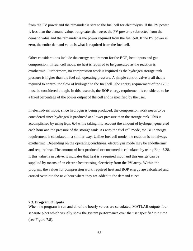
68

from the PV power and the remainder is sent to the fuel cell for electrolysis. If the PV power

is less than the demand value, but greater than zero, the PV power is subtracted from the

demand value and the remainder is the power required from the fuel cell. If the PV power is

zero, the entire demand value is what is required from the fuel cell.

Other considerations include the energy requirement for the BOP, heat inputs and gas

compression. In fuel cell mode, no heat is required to be generated as the reaction is

exothermic. Furthermore, no compression work is required as the hydrogen storage tank

pressure is higher than the fuel cell operating pressure. A simple control valve is all that is

required to control the flow of hydrogen to the fuel cell. The energy requirement of the BOP

must be considered though. In this research, the BOP energy requirement is considered to be

a fixed percentage of the power output of the cell and is specified by the user.

In electrolysis mode, since hydrogen is being produced, the compression work needs to be

considered since hydrogen is produced at a lower pressure than the storage tank. This is

accomplished by using Eqn. 6.4 while taking into account the amount of hydrogen generated

each hour and the pressure of the storage tank. As with the fuel cell mode, the BOP energy

requirement is calculated in a similar way. Unlike fuel cell mode, the reaction is not always

exothermic. Depending on the operating conditions, electrolysis mode may be endothermic

and require heat. The amount of heat produced or consumed is calculated by using Eqn. 5.28.

If this value is negative, it indicates that heat is a required input and this energy can be

supplied by means of an electric heater using electricity from the PV array. Within the

program, the values for compression work, required heat and BOP energy are calculated and

carried over into the next hour where they are added to the demand curve.

7.3. Program Outputs

When the program is run and all of the hourly values are calculated, MATLAB outputs four

separate plots which visually show the system performance over the user specified run time

(see Figure 7.8).

69

Figure 7.8: System performance output screen (Run time ~= 7 months)

In the system performance output screen, the plots represent: the solar resource impinging

upon the PV array, the PV array electrical energy production, the fuel cell energy production

or consumption, the electric demand, the amount of hydrogen in storage, and the amount of

surplus or deficit energy of the system. In all of the plots, the x-axis represents the time in

hours with zero corresponding to the starting simulation time as chosen by the user. In the

second plot, the total power out of the PV array is shown alongside the activity of the

reversible fuel cell and the demand curve. The hydrogen plot shows the amount of hydrogen

in the storage tank over time, in kilograms. In this trial it can be seen that the system is

improperly sized because at the end of the simulation, the hydrogen tank runs empty. This is

also reflected in the surplus/deficit plot as an energy deficit. Also notice how there is a

surplus near the beginning of the simulation. This is because the hydrogen tank is full so no

electrolysis can be carried out even with surplus sunshine.

70

Zooming in on these plots better shows the PV/regenerative fuel cell performance curve, as

seen in Figure 7.9. The PV array output, fuel cell activity and electric demand are shown in

red, green and blue, respectively. The fuel cell activity plot varies from positive values to

negative values to reflect fuel cell mode and electrolysis mode, respectively. It can be seen

that when the PV array power output is greater than the demand curve, electrolysis is

initiated and the fuel cell activity curve goes negative. When this occurs, hydrogen is being

added to the tank which can be seen in the hydrogen plot as a positive slope. When no

sunshine is impinging upon the PV array, the fuel cell activity curve goes positive to meet the

demand curve. Hydrogen is being consumed here and is reflected in the hydrogen plot by a

negative slope. The fuel cell curve (in fuel cell mode) usually rises higher than the demand

curve. This is because extra energy is required to run the BOP so the fuel cell must produce

more energy than simply required by the demand load. When there is not enough sunshine to

trigger electrolysis, it can be seen that the PV array curve and the fuel cell curve work in

tandem to match the demand as is seen during sunrise and sunset.

Several others outputs are displayed in the MATLAB command line. These are shown in

Figure 7.10 and include several total values for the entire simulation run time such as the

amount of solar energy impinging on the panels, the total electrical energy leaving the panels,

amount of hydrogen produced and consumed, total surplus and deficit energies, the percent

of demand that was met, and several others.

These values are useful in properly sizing the power plant. The percentage of demand met

value is especially important in order to determine if the system is large enough. By looking

at the value for total deficit electrical energy, it can be determined if the system is too small.

71

Figure 7.9: System performance output screen zoomed in.

Figure 7.10: Example of MATLAB command line outputs.

72

7.4. Running Multiple Results Simultaneously

Once the program has run one time, it is simple to run off multiple results for various tank

sizes and the number of PV modules. By making modifications to the m-file

“Automation.m,” the user can run quickly run off several different cases very quickly.

Several of the calculations do not need to be recalculated. The cases are automatically saved

as MAT-files. Figure 7.11 shows this m-file where the necessary lines that need to be

modified are highlighted.

Figure 7.11: Screenshot of the “Automation.m” file for running multiple results.

To begin, change line 10 to whatever filename is desired for these trails. The number of PV

modules and the tank size for each run will be attached to the end of this name for each trial.

Line 12 should consist of all of the tank sizes that are to be simulated in kilograms. Any

number of tank sizes can be specified. Line 20 should be changed to specify the PV module

numbers that are to be simulated. In Figure 7.11, line 20 reads “for r=20;10;100.” This will

result in one trial being run for 20 modules, then that number is stepped up to 40 (step

size=20), then 60… all the way to 100. This will be done for each tank size specified. In this

example, a total of 20 trials will be run. Line 13 can be modified in order to properly display

73

a status bar telling the user how far the program has progressed while running. The numbers

“100,” “20” and 10” refer to the upper PV module number limit, the lower PV module

number limit and the step size respectively. When these changes are made, the m-file should

be saved and run. The trials will be saved to the same folder as the run files, and if desired,

the user can open the variable “DemandMatrix” found in the MATLAB workspace to view a

matrix displaying the values for percentage of demand met for all of the trials.

74

Chapter 8 – Component Sizing

When designing a solar-fuel cell-hydrogen power plant, proper equipment sizing is essential

for two main reasons. If any of the components are undersized, the system will be unable

meet the demand loads. If it is oversized, it will be unnecessarily costly. In general, there are

two ranges in scale to look at when studying the system performance curves: microscale and

macroscale. Microscale refers to the trends that occur on an hourly basis over the course of

one day or a few days. Macroscale refers to trends on the order of months or years. This

section analyzes some of these trends.

8.1. Microscale Phenomena

By zooming in on the system performance curve and looking at hourly performance over a

day or week, it is sometimes apparent what system components may be undersized or

oversized. To begin, consider Figure 8.1, which is a simulation with proper component sizes

over the run time of 7 days: 100% of the demand is met. In this simulation, a constant 2 kW

demand load is specified.

In this simulation, there are no energy deficits as indicated in the fourth plot. There exists

some surplus shortly after the start of the simulation, because the hydrogen tank is near full

levels so electrolysis shuts down. Some surplus is usually inevitable as the hydrogen levels

will trend towards peak capacity with a properly sized system, especially when the solar

resource is strong. When there is excess power from the PV array, electrolysis starts and runs

until the PV array power output drops below the demand curve. The fuel cell runs during the

night to meet the demand. There may be a slight downward trend in the hydrogen levels, but

for this run time of 7 days, this is acceptable.

When the PV array is too large, as is shown in Figure 8.2, several trends can be observed

which indicate this is the case. First, it should be seen that there are large amounts of surplus

75

energy during the day, as seen in the fourth plot. Furthermore, it is also observed that

electrolysis starts each day, but then abruptly stops. This is because the hydrogen tank

quickly fills up and electrolysis shuts off, as no more hydrogen is capable of being stored.

When the PV array is too small, as shown in Figure 8.3, it can be seen that the PV array

power rarely passes above the demand curve. As such, electrolysis does not occur often.

Hydrogen is consumed, but rarely produced, so the hydrogen levels quickly trend downward.

It can be seen that once the hydrogen tank runs dry, large deficits are realized. In fact, if no

hydrogen was being produced during the day, the deficit plot would match the demand curve

(at night) when the tank runs empty. The fuel cell is able to run during the night, but only

until the tank runs empty. For most days, the regenerative fuel cell is running in fuel cell

mode during the daytime, dipping in output while the PV array is producing power, which is

not ideal as the regenerative fuel cell should be running in electrolysis mode during the day.

When the hydrogen tank is too small, as in Figure 8.4, three of the plots indicate this is the

case. Most telling is the hydrogen storage plot. It can be seen that when the system is in fuel

cell mode, the hydrogen tank quickly runs empty over the night. The fuel cell shuts down and

electric deficits are observed in the fourth plot. During the day, while generating hydrogen,

the tank quickly fills up and electrolysis stops, as can be seen in the second plot. Also,

surpluses are observed in the fourth plot.

76

Figure 8.1: A properly sized system.

Figure 8.2: A system with too large of a PV array.

77

Figure 8.3: A system with too small of a PV array.

Figure 8.4: A system with too small of a hydrogen tank.

78

When the fuel cell is too small, as seen in Figure 8.5, it can be observed that during the

nighttime the fuel cell curve does not reach the demand curve. In this example a 1 kW fuel

cell was used to try to meet the 2 kW demand curve. The fuel cell is running at maximum

power during the night. Even though there is enough hydrogen in the hydrogen tank, the fuel

cell cannot run at a high enough power to meet the demand, so a deficit shows up in the

fourth plot. The surplus seen in the beginning of the simulation is due to the fact that the

hydrogen tank is full over those hours, so electrolysis shuts down. If the fuel cell were

severely undersized, the fuel cell curve while in electrolysis mode (negative values) would

appear flat as it would max out at its maximum power similar to when it maxes out in fuel

cell mode.

Figure 8.5: A system with too small of a fuel cell.

79

8.2. Macroscale Phenomena

At the macroscale levels (on the order months or years), the main indicator of system

performance comes from observing the hydrogen storage levels. Figure 8.6 shows a three

year simulation for a typical 2 story house in Yuma, AZ. This system is sized adequately

with 115 PV modules, a 25 kg hydrogen tank and a 20 kW fuel cell. 100% of the demand is

met. The hydrogen levels dip in the summer (when the demand is highest) but never reach

zero.

Figure 8.7 shows a system that is too small. There are too few PV modules and the hydrogen

generation is not great enough to keep the tank from running dry. Large deficits are observed

when the tank is near empty.

Figure 8.8 shows a system that is sized too large with too many PV modules. All of the

demand is met, but the hydrogen levels stay at near maximum all year round and huge

surpluses are realized. If the number of PV modules was reduced, the demand could still be

met similar to Figure 8.6. The system size (and cost) could be reduced without affecting

system performance.

80

Figure 8.6: A system that is adequately sized.

Figure 8.7: A system that is sized too small.

81

Figure 8.8: A system that is sized too large.

82

Chapter 9 – House Size Demand Load Results

In the following trials, the goal was to investigate the effects of location and energy

efficiency on the sizing of the system components for the solar-hydrogen power plant. In

order to do this, the program eQUEST was used to design and simulate two houses of similar

construction: a base house and an energy efficient house. The efficient house has the same

dimensions and design as the base house, but with several energy efficient upgrades to

reduce the energy consumption by about half. eQUEST is capable of generating hourly

demand data for one year, which can be loaded into the MATLAB code for the solar-

hydrogen power plant. Yuma and Dayton were selected as the trial locations for two reasons.

The first reason is that Yuma possesses an excellent solar resource while Dayton has only a

modest solar resource. The second reason is the two locations have different cooling and

heating demands based on their local environments. Once these demand curves were

generated and input into the MATLAB program, several data runs were performed while

specifying different equipment sizes. Results from these runs were plotted and evaluated.

9.1. eQUEST House Specifications

eQUEST is an energy simulation tool for houses and buildings designed for the Department

of Energy. It is the successor to the DOE-2 building simulation software that has a very user

friendly graphical user interface (GUI) and more in depth modeling parameters. By

specifying properties such as building location, size, construction type, building materials,

internal loads, lighting specifications, etc., eQUEST then takes into account the local weather

data by using DOE-2/eQUEST bin files to calculate heat flows, electric consumption, etc.

These weather files contain meteorological data such as outdoor air temperature, relative

humidity, wind speed, solar irradiance and more, which is essential in modeling heat flows

into and out of building structures. By calculating these heat flows, and by specifying the

heating and cooling systems for a building or house, the total energy demand over the course

of one year can be calculated with fair accuracy. Ideally, the results could then be calibrated

83

to actual data from an existing structure. For this research, the no calibration was performed

as there was no physical house to compare to.

A base house was created in eQUEST with standard efficiency building materials which is

supposed to represent a typical, two story house in the United States. This base house has a

footprint of 35 ft by 35 ft with two floors for a total area of 2,450 ft2. There is no basement

and the house has a slab-on-grade foundation. Each floor has an 8 ft ceiling with a 1 ft space

between the ceiling of the ground floor and bottom of the top floor. So that the energy

demand of the house can be met with the electric solar-fuel cell-hydrogen power plant, the

houses were converted to all electric. Several of the base house‟s specifications that are

required by eQUEST are given in Table 9.1.

Table 9.1: Some of the base house specifications used in the eQUEST simulation.

Window area = 10% of each wall ACHhouse = 0.30 air changes per hour

Rwalls = 9 hr-ft2-F/Btu Qelec,avg = 1.7955 W/ft2

Rwindows = 1 hr-ft2-F/Btu (single pane) Occupancy schedule: 7PM - 8AM weekdays, all day on weekends

Rceiling = 12 hr-ft2-F/Btu Tia = 72 F (winter), 75F (summer)

Rroof = 3 hr-ft2-F/Btu 2 wooden doors, one north side, one south side

SHGCnormal = 0.9 COP heat pump = 2.81

Solar absorptivity walls = 0.6 SEER-air conditioner = 9.7 Btu/W-hr

Solar absorptivity roof = 0.9 hexterior,avg = 5 Btu/hr-ft2-F

Rfloor = 1 hr-ft2-F/Btu No overhangs over windows

Rslab,perim = 5 hr-ft2-F/Btu Qlighting,avg = 1.045 W/ft2

Frame type = 2x4 16” on center studs HVAC type: Air source heat pump

Domestic water heater setpoint: 140 F Economizer: None

Supply Fan Type: Constant

A schematic of the base house was created using Google SketchUp and is shown in Figure

9.1. The dimensions are to scale and the colors approximately represent how light and dark

the exterior surfaces are.

84

Figure 9.1: Schematic of the base house.

After this base house was designed in eQUEST, an energy efficient house was generated by

making several upgrades to the structure in order to reduce the total electric demand by about

half. Some of these upgrades are:

- Window upgrades were made which included using low emissivity, argon-

filled, double pane windows which have a lower thermal conductivity than the

base house‟s windows. Overhangs of 4 ft were added to the south, east and

west sides to minimize the beam radiation into the house during the summer

which subsequently reduces the cooling load.

- Daylighting controls were implemented to reduce the lighting loads required

at certain times of the day. This upgrade includes the use of photosensors and

dimming controls. The minimum required luminescence was set at 35 foot-

candles.

- The absorptivity of the roof was reduced from 0.9 to 0.4 which has the effect

of reducing the solar roof temperature, especially during the summer months.

This can be accomplished by installing new shingles or using special paints of

lighter colors.

- Insulation was thickened or upgraded throughout the house. This included

adding more fiberglass batt insulation to the walls, top floor ceiling and roof.

Closed cell foam, polyisocyanurate (polyiso), was added the walls and floor.

85

- The type of framing used in the exterior walls was upgraded from 2x4 studs

with 16” spacing to 2x6 studs with 24” spacing. By adding more space

between the studs, thermal bridging was reduced and by using 2x6 studs

instead of 2x4, more space is available for insulation.

- The infiltration rate was reduced from 0.3 ACH to 0.2 ACH. Keeping the

conditioned air inside and the unconditioned air outside reduces loads on the

heating and cooling system.

- The internal electric loads were reduced by about one-third compared to the

base house. This can be accomplished by using more energy efficiency

appliances and light bulbs for example.

- By adjusting the unoccupied setpoints on the thermostat, less energy can be

used throughout the year. The unoccupied cooling setpoint was increased by

2˚F and the heating setpoint increased by 4 ˚F. The set point on the hot water

supply was also reduced from 140 ˚F to 120 ˚F. Furthermore, the cooling

supply air temperature and heating supply air temperature setpoints were

changed from 55 ˚F to 60 ˚F and 90 ˚F and 85 ˚F, respectively.

- The heat pump/air conditioning unit of the base house was replaced with a

more efficient one. The SEER of the AC was increased from 9.7 to 12 while

the COP of the heat pump was increased from 2.81 to 5.

Several of the efficient house‟s specifications that are required by eQUEST are given in

Table 9.2.

86

Table 9.2: Some of the efficient house specifications used in the eQUEST simulation.

Window area = 10% of east and west walls,

20% of north and south walls

Qelec,avg = 0.943W/ft2

Rwalls = 29 hr-ft2-F/Btu Occupancy schedule: 7PM - 8AM weekdays, all day on weekends

Rwindows = 2.68 hr-ft2-F/Btu (double pane), east, west,

south, 1.85 hr-ft2-F/Btu north

Tia = 72 F (winter), 75 F (summer)

Rceiling = 45 hr-ft2-F/Btu 2 wooden doors, one north side, one south side

Rroof = 29 hr-ft2-F/Btu COP heat pump = 5

SHGCnormal = 0.9 SEER-air conditioner = 12 Btu/W-hr

Solar absorptivity walls = 0.4 hexterior,avg = 5 Btu/hr-ft2-F

Solar absorptivity roof = 0.4 4ft overhang 0.5 ft above the east, west and south windows

Rfloor = 7, Rslab,perim = 10 hr-ft2-F/Btu Qlighting,avg = 0.62 W/ft2

Frame type = 2x6 24” on center studs HVAC type: Air source heat pump

Domestic water heater setpoint: 120 F Economizer: Drybulb temperature, high limit: 65 F

Daylighting: 35 foot-candle minimum, dimming down to

10% light

Supply fan type: Variable speed drive

ACHhouse = 0.20 air changes per hour

A diagram of the energy efficient house was also created using Google SketchUp and can be

seen in Figure 9.2. Dimensions are to scale and colors are approximated to represent how

light and dark the exterior surfaces are.

Figure 9.2: Schematic of the efficient house.

9.2. House Size Demand - Results

After these two houses were planned and designed, the data was input into eQUEST along

with the location and weather data to generate four separate demand curves (see Figures 9.3

87

to 9.6). As can be seen in both locations, the efficient house uses about half as much energy

as the base house. Note that in Dayton the highest demand is seen during the winter months

as more heating is required. In Yuma, the highest demand is seen in the summer when

cooling is required. For the maximum, minimum and average demand values for these four

loads refer to Table 9.3.

After these demand curves where generated, they were then input into the MATLAB

program for the solar-fuel cell-hydrogen power plant. Several trials were run with different

system sizes. For these trials, the default values of the program were specified. For the PV

modules, SolarWorld SW 270 modules were used which have a maximum power output of

270 W. The number of modules selected was varied for each case. The panel tilt was set to

31˚ for Yuma and 38˚ in Dayton. For all four cases, a 20 kW fuel cell size was used for a

more direct comparison. The hydrogen tank size was varied between the following sizes: 12,

25, 50, 100 and 200 kg.

Figure 9.3: Base house electric demand for Dayton, OH.

88

Figure 9.4: Efficient house electric demand for Dayton, OH.

Figure 9.5: Base house electric demand for Yuma, AZ.

89

Figure 9.6: Efficient house electric demand for Yuma, AZ.

Table 9.3: Electric demand properties for both houses in Dayton and Yuma.

House type (location) Maximum demand Minimum demand Average demand

Base house (Dayton, OH) 20.91 kW 0.65 kW 4.06 kW

Efficient house (Dayton, OH) 12.53 kW 0.31 kW 2.04 kW

Base house (Yuma, AZ) 13.92 kW 0.64 kW 4.00 kW

Efficient house (Yuma, AZ) 6.86 kW 0.30 kW 2.22 kW

A few of the MATLAB program‟s outputs are shown in Figures 9.7 through 9.10. The first

two show results for the efficient house in Yuma. In Figure 9.7, the system is adequately

sized with 54 PV modules, a 20 kW fuel cell and a 25 kg hydrogen tank. There is a

noticeable dip in the hydrogen storage level during the summer months which is due to the

fact that the electric demand increases greatly because of the hot summer weather. In Figure

9.8, the system is undersized with 45 PV modules, a 20 kW fuel cell and a 25 kg hydrogen

tank. As can be seen, the hydrogen storage levels take a dip during the summer months when

90

the cooling demand is highest and large electricity deficits are realized because the hydrogen

tanks run dry. Figure 9.9 shows the efficient house in Dayton, OH, using 207 PV modules, a

20 kW fuel cell and 25 kg of hydrogen storage. This system is adequately sized. Figure 9.10

shows the same house with 88 PV modules, a 20 kW fuel cell and a 25 kg hydrogen storage

tank. It can clearly be seen that during the winter months, the system is unable to produce

enough hydrogen so the tank empties and electricity deficits are observed.



demand is met.

91


operation with 45 PV modules, a 20 kW fuel cell and 25 kg hydrogen storage. About

96% of the demand is met.


operation with 207 PV modules, a 20 kW fuel cell and 25 kg hydrogen storage. All of

the demand is met.

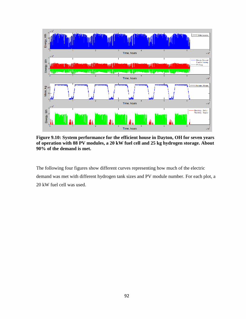
92

Figure 9.10: System performance for the efficient house in Dayton, OH for seven years

of operation with 88 PV modules, a 20 kW fuel cell and 25 kg hydrogen storage. About

90% of the demand is met.

The following four figures show different curves representing how much of the electric

demand was met with different hydrogen tank sizes and PV module number. For each plot, a

20 kW fuel cell was used.

93

Figure 9.11: Percentage of demand met vs. component sizes for base house in Dayton,

OH.

Figure 9.12: Percentage of demand met vs. component sizes for efficient house in

Dayton, OH.

94

Figure 9.13: Percentage of demand met vs. component sizes for base house in Yuma,

AZ.

Figure 9.14: Percentage of demand met vs. component sizes for efficient house in Yuma,

AZ.

95

As can be seen between the base house and energy efficient house in both locations, energy

efficiency is an extremely important consideration when designing a solar-fuel cell-hydrogen

power plant. For example, in Dayton with the base house, when using a 100 kg hydrogen

storage tank and a 20 kW fuel cell, in order to meet 100% of the demand, more than 600 PV

modules are required. With smaller hydrogen storage tanks, the demand is unable to be met

completely, but after the energy efficiency upgrades are made, the required number of PV

modules drops to around 100. In Yuma when using a 20 kW fuel cell and a 100 kg hydrogen

tank with the base house, somewhere around 100 PV modules are required to meet 100% of

the demand. When energy efficiency upgrades are made, about 50 PV modules are enough to

completely cover the demand. The difference in system sizing between the base house and

the efficient house are striking and should highlight the importance of energy efficiency in

reducing the size of solar-fuel cell-hydrogen power plants.

One discrepancy that should be pointed out is that in the plots for the base house in Dayton,

OH (Figure 9.11) it appears that the curve for 100 kg of hydrogen storage reaches 100% but

then drops by a very small amount as the number of PV modules increases further. This is an

artifact from how the program calculates and accounts for the heat requirement and

compression work for when the fuel cell is in electrolysis mode. For each hour, the amount of

heat and the compression work required is calculated and accounted for in the subsequent

hour by essentially adding it to the demand value of the next hour. This is done because both

the heat requirement and compression work is a function of the power into the fuel cell and

the amount of hydrogen produced. By accounting for these energy requirements in the

subsequent hour, complex solver routines can be avoided which would otherwise introduce

thousands of solver routines with significant probabilities of failing to converge. The

program is thus more robust. With large run times and small step sizes, this method has

minimal effect on program accuracy. The reason the artifact exists is because with large

numbers of PV modules there are times where several thousand kilowatt hours of power are

sent to the electrolyzer cell and when the energy requirements are calculated in the

subsequent hour, either the fuel cell power maxes out if the next hour requires fuel cell mode

or the PV array does not put out enough power to pay for all of the energy requirements, so a

small amount of energy deficit is seen in a few of the hourly calculations.

96

Besides the fact that Yuma has a much better solar resource than Dayton, one of the reasons

the Dayton system is required to be so much larger than the Yuma system is the shape of the

demand curve in reference to the solar resource throughout the year. In Yuma, the demand

loads are the highest in the summer when the solar resource is strongest. But in Dayton, due

to colder winters, the demand load is highest in the winter when lots of heating is required.

This mismatch between peak demand loads and peak solar resource loads results in the need

for a significantly larger solar-hydrogen power plant.

Another finding from this study was that as the hydrogen tank size was increased, the

required number of PV modules decreased. With more storage, the system can run longer

without adequate solar resource, and less solar energy is wasted when the solar resource is

good, because the tank can continue to fill for longer periods of time. In Dayton, with the

base house, a 100 kg tank required over 600 modules to reach nearly 100% demand

coverage, but that number dropped to about 375 modules when a 200 kg tank was

considered. This is partly attributed to the fact that when the tank size is very large, hydrogen

that was stored during the summer can be carried over into the winter months. In Yuma, the

tank size has less of an effect because the solar resource is good even in the winter and

because of the better matching between the demand load and the solar resource.

97

Chapter 10 – Effects of Fuel Cell Size on System

Performance In this series of trials, it was desired to explore the effects of the fuel cell size on the

performance of a solar-fuel cell-hydrogen power plant. In order to meet 100% of the demand

load, it is necessary that the fuel cell system be large enough to meet the maximum power

value of the demand. Upon initial inspection, it may seem that if the fuel cell is large enough

to meet the maximum demand, then no benefit may be derived from increasing its size.

However, this will be shown to not be true, because the efficiency of a fuel cell in operation

is largely dependent upon the current density of the fuel cell. For a constant stoichiometry

flow rate, a fuel cell is most efficient at lower current densities. This is demonstrated in

Figure 10.1.

In order to explore the effects of fuel cell size on system performance, a constant 2 kW

demand load was specified and Yuma, AZ, was selected as the location. The type of PV

module that was selected was a SolarWorld SW 270 that has a maximum power rating of

270 W. For these trials, the number of modules was varied between 15 and 225 and the

hydrogen storage sizes that were used were 12, 25, 50 and 100 kg. Three different

regenerative fuel cell sizes were selected: 2.5, 5 and 10 kW in fuel cell mode.

Figures 10.2 through 10.4 show the system performances for the three different fuel cell

sizes, all using 55 PV modules and 25 kg of hydrogen storage in the system.

98


methods. For constant stoichiometry =1 and for constant flow rate, 1.1 times the

required flow rate at maximum current density is supplied.

Figure 10.2: System performance curves using a 2.5 kW fuel cell, 55 PV modules and 25

kg of hydrogen storage. Run time is seven years.

99

Figure 10.3: System performance curve using a 5 kW fuel cell, 55 PV modules and 25


Figure 10.4: System performance curve using a 10 kW fuel cell, 55 PV modules and 25


100

As can be seen, with the 2.5 and 5 kW fuel cell, the demand could not be met with 55

modules and 25 kg of hydrogen storage. However, when a 10 kW fuel cell is used, the

demand was easily met with significant surplus energy generated.

By varying the number of PV modules and the hydrogen storage size as mentioned above,

the following three plots were generated which relate the percentage of the demand met with

PV module number and hydrogen storage. As can be seen from Figures 10.5 through 10.7,

increasing the size of a fuel cell in a given system means the number of PV modules can be

reduced while still meeting all of the electricity demand. This is because the fuel cell can

effectively run in a more efficient region on the current-power curve. For example, when

specifying a 10 kW fuel cell, less than 60 PV modules are required for any of the hydrogen

tank sizes selected. But if a 2.5 kW fuel cell is used, around 130 PV modules are needed if

the tank size is 12 kg, or if a 100 kg tank is used a little over 90 modules are required. With a

100 kg tank and a 10 kW fuel cell, the demand can be met with around 40 modules. These

results clearly demonstrate the importance of fuel cell size on system performance. Using a

larger fuel cell allows for the other system components to be reduced in size. Looking at this

from another angle, upgrading the fuel cell in an undersized system can allow the system to

be properly sized without changing the hydrogen storage capacity or the number of PV

modules.

101

Figure 10.5: Percentage of demand met vs. different component sizes for a 2.5 kW fuel

cell.

Figure 10.6: Percentage of demand met vs. different component sizes for a 5 kW fuel

cell.

102

Figure 10.7: Percentage of demand met vs. different component sizes for a 10 kW fuel

cell.

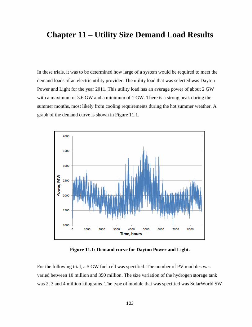
103

Chapter 11 – Utility Size Demand Load Results

In these trials, it was to be determined how large of a system would be required to meet the

demand loads of an electric utility provider. The utility load that was selected was Dayton

Power and Light for the year 2011. This utility load has an average power of about 2 GW

with a maximum of 3.6 GW and a minimum of 1 GW. There is a strong peak during the

summer months, most likely from cooling requirements during the hot summer weather. A

graph of the demand curve is shown in Figure 11.1.

Figure 11.1: Demand curve for Dayton Power and Light.

For the following trial, a 5 GW fuel cell was specified. The number of PV modules was

varied between 10 million and 350 million. The size variation of the hydrogen storage tank

was 2, 3 and 4 million kilograms. The type of module that was specified was SolarWorld SW

104

270 with a maximum power rating of 270 W. The results for Dayton, OH over these ranges

are shown in Figure 11.2.

Figure 11.2: Percentage of demand met vs. system component sizes in Dayton, OH using

a 5 GW fuel cell.

These results show that in order to meet most of Dayton Power and Light‟s electric demand

load (~99%), about 200 million solar modules are required along with a 2 to 3 million

kilogram hydrogen storage tank using a 5 GW fuel cell. Notice that a 5 GW fuel cell does not

cover 100% of the demand because when the energy demands of the BOP are taken into

account, the effective demand surpasses 5 GW in some instances. Since the SolarWorld

modules have an area of about 1.67 m2, the total surface area of PV panel required to meet

about 98% of the demand comes out to 128 square miles. This is a rather large surface area

and it would likely be hard to find a place near Dayton, OH to set up such a solar field.

In order to determine how large the PV array would have to be if the solar resource was very

good, the same demand load was powered by placing the PV array in Yuma, AZ. Yuma has

an excellent solar resource and plenty of unused land nearby (desert) to place such a solar

105

field. In order to visualize such a scenario, it could be imagined that the PV array is located

in Yuma, AZ with the array‟s electrical output sent to Dayton by high-voltage transmission

lines where the fuel cell system and hydrogen storage tank would be located. While this

simulation does not take into account transmission losses, the importance of the solar

resource is still represented in this trial. Figure 11.3 shows the results.

Figure 11.3: Percentage of demand met vs. system component sizes when the PV array

is located in Yuma, AZ and the fuel cell system and hydrogen storage tank are placed in

Dayton, OH. A 5 GW fuel cell is used.

As can be seen, all of the load could be powered in Yuma, AZ by using about 100 million PV

modules. This reduces the required surface area of the PV array to about 65 square miles.

This PV array would be about 50% of the size of the array if it were located in Dayton, OH.

Next it was desired to determine how much smaller the PV arrays could be if a larger fuel

cell was used. The 5 GW fuel cell was replaced with a 25 GW fuel cell. The results for

Dayton, OH are shown in Figure 11.4.

106

Figure 11.4: Percentage of demand met vs. system component sizes in Dayton, OH using

a 25 GW fuel cell.

When the fuel cell size is increased to 25 GW, it can be seen that about 150 million PV

modules are required to meet about 99% of demand. This reduces the surface area of the PV

array to about 97 square miles as compared to 128 square miles for the case with a 5 GW fuel

cell. A trial was also run for the case where the PV array was located in Yuma and the fuel

cell was upgraded to a 25 GW fuel cell. These results are shown in Figure 11.5.

The number of PV modules drops to about 80 million. The results in a total PV array surface

area of about 52 square miles. While these surface areas may seem astronomical, unused

dessert land may be ideal for placing large solar fields as they are rarely used for other

purposes and the price of land in the desert should be much cheaper than near more

populated areas such as Dayton, OH. An area of 52 square miles would encompass about

0.04% of Yuma‟s total surface area. Furthermore, these surface areas will be reduced as

module efficiency inevitably increases in the future. For example, if the efficiency of PV

modules doubles in the future, which seems plausible given that today‟s commercial modules

107

generally have efficiencies of less than 20% (there is much room for improvement), the total

surface area required if the PV array were placed in Yuma (and a 25 GW fuel cell were used)

could drop to around 20 square miles. These results highlight the importance of placing

larger solar fields in areas with good solar resource and also the importance of increasing

module efficiency with continued research and development.

Figure 11.5 Percentage of demand met vs. system component sizes when the PV array is


Dayton, OH. A 25 GW fuel cell is used.

While hydrogen storage capacities in the millions of kilograms seems especially large, it

should be noted that these storage sizes are not unattainable. For example, the

ConocoPhillips Clemens Terminal in Texas has successfully stored hydrogen in a solution-

mined salt cavern with a total usable volume of about 1066 million stand cubic feet or about

2.5 million kilograms of hydrogen storage capacity [Forsberg, C.W (2006)].

108

Another consideration is that with large solar-fuel cell-hydrogen power plants such as these,

it is important not to neglect the amount of surplus electrical energy created by the system.

For example, with a 25 GW fuel cell, 3 million kilograms of hydrogen storage, 70 million

modules and with the PV array placed in Yuma, the total amount of surplus energy was

found to be about 55 GWh over three years. If this could be sold at a rate of $0.1/kWh to the

grid, around 1.8 million dollars could be generated annually; not an insignificant amount.

Three system performance curves are shown for Yuma, AZ (Figures 11.6 to 11.8) when

using a 25 GW fuel cell and a 2 million kilogram hydrogen storage tank showing an

undersized system, an oversized system and a system that is properly sized. The undersized

system included 25 million PV modules, the oversized system uses 190 million PV modules

and the properly sized system uses 115 million PV modules. The 25 million module system

is clearly undersized as the hydrogen levels drop to zero in some places. The 190 million

module system is oversized because, although it does meet all of the demand, the demand

can be met with a smaller number of modules as is shown with the 115 million module

system.

Three system performance curves are also shown for Dayton, OH (Figures 11.9 to 11.11)

also using a 25 GW fuel cell and 2 million kilograms of hydrogen storage. The number of PV

modules that are used is 65, 185 and 410 million, respectively.

109

Figure 11.6: System performance when the PV array is located in Yuma, AZ and the

fuel cell system and hydrogen storage tank are placed in Dayton, OH. A 25 GW fuel cell

is used along with 2 million kg of hydrogen storage and 25 million PV modules. This

system is clearly undersized with just 72.7% of the demand met. Run time is seven

years.




system is oversized because the demand can be met with fewer panels (See Figure 11.8)

and the electricity surplus can be reduced. Run time is seven years.

110




system is properly sized with 100% of the demand met. Run time is seven years.

Figure 11.9: System performance when the system is placed in Dayton, OH. A 25 GW

fuel cell is used along with 2 million kg of hydrogen storage and 65 million PV modules.

This system is clearly undersized with 88.8% of the demand met. Run time is seven

years.

111

Figure 11.10: System performance when the system is placed in Dayton, OH. A 25 GW fuel cell

is used along with 2 million kg of hydrogen storage and 185 million PV modules. This system is

slightly undersized with 98.9% of the demand met. Run time is seven years.

Figure 11.11: System performance when the system is placed in Dayton, OH. A 25 GW

fuel cell is used along with 2 million kg of hydrogen storage and 410 million PV

modules. This system is properly sized with 100% of the demand met. Run time is seven

years.

112

Chapter 12 – Summary and Conclusions

The major thrust of this work was the development of a computer program that simulates the

performance of a 24-hour solar-fuel cell-hydrogen electric power plant. One of the primary

purposes of developing this computer model was to see how large such a power plant would

have to be to meet a given electrical demand, in a given location, with solar power as the

only energy input. Of course to do this, some sort of energy storage technique is required, as

well as a mechanism to convert that stored energy into electricity. For this research, the type

of energy storage chosen was compressed hydrogen gas, and the device used to convert

electrical energy into chemical energy, and vice versa, was a regenerative fuel cell. Thus the

computer program that was developed includes several detailed models so that the overall

performance of a this power plant can be determined.

The first detailed model included in the computer code is that of the solar resource. This

model is such that it can determine the amount of solar energy impinging on a surface at a

given location, at a given time, for a given orientation. It includes the direct beam radiation

striking this surface as well as the diffuse and reflected components striking the surface. The

diffuse component is broken into three parts: an isotropic component, a circumsolar

component, and a horizon brightening component. Essentially the solar resource is calculated

in detail as a function of the time of day and the day of the year for the location and

orientation of the photovoltaic panels.

A second detailed mathematical model included in the 24-hour solar-fuel cell-hydrogen

electric power plant computer program is that of the photovoltaic modules themselves. This

model is needed to determine how much of the solar resource impinging on the photovoltaic

panels is converted into electricity. This is done using a four parameter model for the

specified photovoltaic modules. A lumped circuit representation of the photovoltaic modules

includes a current source, a diode, and a series resistance that is used to model the

photovoltaic panel. Four equations describing the performance of this circuit model at three

113

different points on the operating curve are used to fit the I-V characteristic equation to a

particular photovoltaic modules. With this particular I-V characteristic equation, the

electrical power out of the photovoltaic module is determined for any given solar irradiance

and cell temperature. Using a maximum power point tracker, the modules are forced to

operate at their maximum power production current and voltage.

A third detailed mathematical model included in this program is that of the regenerative fuel

cell. This model accounts for the fuel cell operating in the forward mode and the reverse

mode. In the forward operation mode, hydrogen is consumed and electrical power is

produced; and in the reverse mode, electrical energy is consumed and hydrogen is produced.

Equations were developed for the current-voltage characteristic of the fuel cell, operating in

both modes. Both of these current-voltage characteristics account for the mass transport

overvoltage, the activation overvoltage, and the ohmic overvoltage.

The fourth mathematical model included in this work is that of the amount of work required

to place the hydrogen in storage while tracking the pressure of the storage tank. A simple

ideal gas model is used to do this. The hydrogen storage model is relatively simple as the

amount of hydrogen added to storage or removed from storage is determined by the fuel cell

model of this program.

The computer program developed for simulating this power plant takes the detailed models

for the solar resource, the photovoltaic modules, the regenerative fuel cell, and the hydrogen

storage and combines them into a system simulation that determines the power output of the

system. A detailed hourly tracking of the system is performed relative to an input demand

curve. The computer program constantly adjusts the direction of the solar power to either

meeting immediate demands or producing hydrogen. Only when the power output of the

photovoltaic array exceeds the immediate demand is hydrogen produced and put into storage

for later use. When there is not enough power produced by the solar panels to meet

immediate demand, hydrogen is withdrawn from storage, run through the fuel cell and

converted to electrical energy so the demand is met. If there is not enough photovoltaic-

generated electricity or fuel cell-generated electricity, a power deficit is calculated. If more

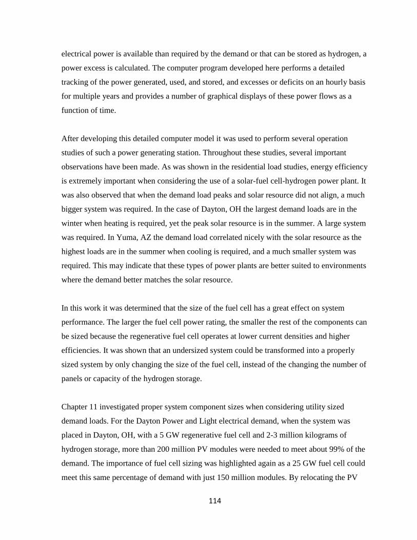
114

electrical power is available than required by the demand or that can be stored as hydrogen, a

power excess is calculated. The computer program developed here performs a detailed

tracking of the power generated, used, and stored, and excesses or deficits on an hourly basis

for multiple years and provides a number of graphical displays of these power flows as a

function of time.

After developing this detailed computer model it was used to perform several operation

studies of such a power generating station. Throughout these studies, several important

observations have been made. As was shown in the residential load studies, energy efficiency

is extremely important when considering the use of a solar-fuel cell-hydrogen power plant. It

was also observed that when the demand load peaks and solar resource did not align, a much

bigger system was required. In the case of Dayton, OH the largest demand loads are in the

winter when heating is required, yet the peak solar resource is in the summer. A large system

was required. In Yuma, AZ the demand load correlated nicely with the solar resource as the

highest loads are in the summer when cooling is required, and a much smaller system was

required. This may indicate that these types of power plants are better suited to environments

where the demand better matches the solar resource.

In this work it was determined that the size of the fuel cell has a great effect on system

performance. The larger the fuel cell power rating, the smaller the rest of the components can

be sized because the regenerative fuel cell operates at lower current densities and higher

efficiencies. It was shown that an undersized system could be transformed into a properly

sized system by only changing the size of the fuel cell, instead of the changing the number of

panels or capacity of the hydrogen storage.

Chapter 11 investigated proper system component sizes when considering utility sized

demand loads. For the Dayton Power and Light electrical demand, when the system was

placed in Dayton, OH, with a 5 GW regenerative fuel cell and 2-3 million kilograms of

hydrogen storage, more than 200 million PV modules were needed to meet about 99% of the

demand. The importance of fuel cell sizing was highlighted again as a 25 GW fuel cell could

meet this same percentage of demand with just 150 million modules. By relocating the PV

115

array to Yuma, AZ and transmitting the electricity through high-voltage transmissions lines,

with a 25 GW fuel cell, the required number of modules to meet all of the demand dropped to

about 70 million.

There are several areas of interest that would be useful to investigate to determine how the

system performance and component sizing might change. When considering the residential-

sized loads, the houses were converted to all-electric because an in-depth study of heat

recovery was not considered in this research. If some of the heat from the fuel cell were used

for the heating requirements of the houses, then it is likely that the system components could

be reduced to some degree. This may be especially true in Dayton where the largest demands

are in the winter when heating is required. Another area of study that might help reduce the

component sizes would be to incorporate another energy source, such as wind power, into

these types of power plants. Currently, at night, the fuel cell must provide all of the power for

the demand. Since wind power is often most prevalent at night, it is possible that the fuel cell

(and possibly other components) could be reduced in size.

In this research a computer model was used to aid in the selection of component sizes for a

24-hour solar-fuel cell-hydrogen electric power plant. Several interesting results were

discovered and highlighted; however, the ultimate feasibility of building and operating these

types of power plants may be heavily dependent on the progress made in the research and

development of the individual system components, with an aim of making them more

efficient, and hence reduce the required sizes of these types of power plants.

As time goes on, power plants such as these may see widespread adoption for several

reasons. The price of renewable energy technology is dropping at alarming rates with solar

photovoltaics already under $1/W and having reached grid parity in many locations. Also

important to note is that once these types of power plants are constructed, they should have

extremely low operating costs as the energy input, sunlight, is free. Furthermore, these types

of electric power plants are attractive because they are environmentally friendly, producing

little to no pollution or greenhouse gases. And finally, the potential for renewable energies

such as solar to scale with increasing energy demands is quite high as a couple hours of

116

sunlight impinging on the earth contains enough energy to meet the world‟s energy demands

for about a year.

117

References

Anderson, D. and Leach, M. Harvesting and redistributing renewable energy: on the role of

gas and electricity grids to overcome intermittency through the generation and storage of

hydrogen. Energy Policy. (2004) Vol. 32, 1603-1614. doi:10.1016/S0301-4215(03)00131-9.

Chan et al. A complete polarization model of a solid oxide fuel cell and its sensitivity to the

change of cell component thickness. Journal of Power Sources. (2001) Vol. 93, 130-140.

Da Rosa, Aldo V. Fundamentals of Renewable Energy Processes. 2nd edition. Academic

Press. (2009).

Duffie, John A., and Beckman, William A. Solar Engineering of Thermal Processes. John

Wiley & Sons. 2nd edition, (1991).

El-Shatter et al. Hybrid PV/fuel cell system design and simulation. Renewable Energy.

(2002) Vol. 27, 479-485. PII: S09 60 -1481(01)00062-3.

Energy Information Administration, United States. International Energy Outlook. (2011)

Forsberg, C.W. Assessment of nuclear-hydrogen synergies with renewable energy systems

and coal liquefaction processes. Oak Ridge National Laboratory. (2006).

Ghosh et al. Ten years of operational experience with a hydrogen-based renewable energy

supply system. Solar Energy. (2003) Vol. 75, 469-478. doi:10.1016/j.solener.2003.09.006.

Kasten, F. and Young, A.T. Revised optical air mass tables and approximation formula.

Applied Optics. (1989) Vol. 28, No. 22, 4735-4738.

Kim et al. Polarization effects in intermediate temperature, anode-supported solid oxide fuel

cells. Journal of the Electrochemical Society. (1999) Vol. 146, No. 1, 69-78.

King, et al. Photovoltaic array performance model. Sandia National Laboratories. (2004).

118

Klell, M. Storage of Hydrogen in the Pure Form. Handbook of Hydrogen Storage, (2010).

Lehman et al. Operating experience with a photovoltaic-hydrogen energy system. Hydrogen

‟94: The 10th World Hydrogen Energy Conference. June 20-24, (1994).

Maclay et al. Dynamic analyses of regenerative fuel cell power for potential use in

renewable residential applications. International Journal of Hydrogen Energy. (2006), Vol.

31, 994-1009. doi:10.1016/j.ijhydene.2005.10.008.

Nelson, Jenny. The Physics of Solar Cells. Imperial College Press, (2004).

Ntziachristos et al. A wind-power fuel-cell hybrid system study on the non-interconnected

Aegean islands grid. Renewable Energy. (2005) Vol. 30, 1471-1487.

doi:10.1016/j.renene.2004.11.007.

O‟Hayre, Ryan, et al. Fuel Cell Fundamentals. 2nd edition. John Wiley & Sons, (2009).

Perez et al. A new simplified version of the Perez Diffuse Irradiance Model for Tilted

Surfaces. Solar Energy. (1987) Vol. 29, 221.

Santarelli, M and Macagno, S. Hydrogen as an energy carrier in stand-alone applications

based on PV and PV-micro-hydro systems. Energy. (2004) Vol. 29, 1159-1182.

doi:10.1016/j.energy.2004.02.023.

Shakya et al. Technical feasibility and financial analysis of hybrid wind-photovoltaic system

with hydrogen storage for Cooma. International Journal of Hydrogen Energy. (2005), Vol.

30, 9-20. doi:10.1016/j.ijhydene.2004.03.013.

Schucan, T. Final report of subtask A: Case studies of integrated hydrogen energy systems.

International Energy Agency (2000).

119

Szyszka, A. Demonstration plant, Neunburg vorm Wald, Germany, to investigate and test

solar-hydrogen technology. International Journal of Hydrogen Energy. (1992) Vol. 17, No. 7,

485-498.

Szyszka, A. Ten years of solar hydrogen demonstration project at Neunburg vorm Wald,

Germany. International Journal of Hydrogen Energy. (1998) Vol. 23, No. 10.

Townsend, T.U. A method for estimating the long-term performance of direct-coupled

photovoltaic systems. (1989) University of Wisconsin – Madison.

Troncoso, E. and Newborough, M. Implementation and control of electrolyzers to achieve

high penetrations of renewable power. International Journal of Hydrogen Energy. (2007)

Vol. 32, 2253-2268. doi:10.1016/j.ijhydene.2007.02.034.

Tsao, J. et al. Solar FAQs, Working Draft Version. (2006)

Vanhanen et al. Operation experiences of a phosphoric acid fuel cell in a solar hydrogen

energy system. International Journal of Hydrogen Energy. (1997) Vol. 22, No. 7, 707-713.

Vanhanen et al. Electrolyzer-metal hydride-fuel cell system or seasonal energy storage.

International Journal of Hydrogen Energy. (1998) Vol. 23, No. 4, 267-271.

Weast. R. C., Handbook of Chemistry and Physics. 53th edition. Chemical Rubber Co.,

(1972).

Young et al. Feasibility of renewable energy storage using hydrogen in remote communities

in Bhutan. International Journal of Hydrogen Energy. (2007) Vol. 32, 997-1009.

doi:10.1016/j.ijhydene.2006.07.002.

120

Appendix A – Tabulated Results for Residential, Baseload and Utility Load Studies

Table A1: Yuma, AZ - 2 kW constant load- 2.5 kW fuel cell (7 years).

121

Table A2: Yuma, AZ - 2 kW constant load - 5 kW fuel cell (7 years).

122

Table A3: Yuma, AZ - 2 kW constant load - 10 kW fuel cell (7 years).

123

Table A4: Dayton, OH – Base house load – 20 kW Fuel cell (7 years).

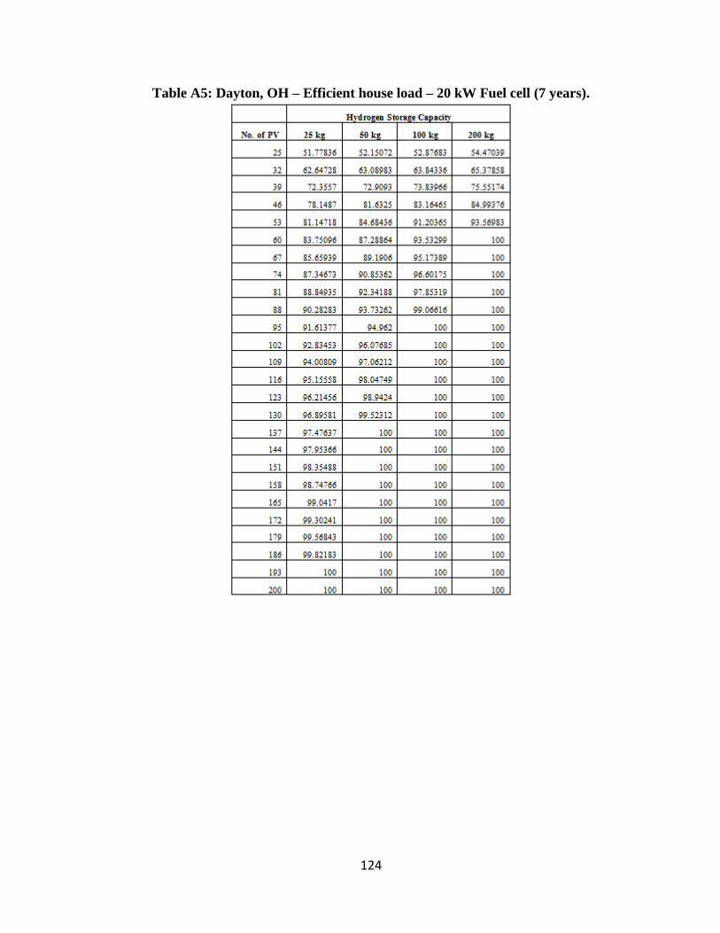
124

Table A5: Dayton, OH – Efficient house load – 20 kW Fuel cell (7 years).

125

Table A6: Yuma, AZ – Base house load – 20 kW Fuel cell (7 years).

126

Table A7: Yuma, AZ – Efficient house load – 20 kW Fuel cell (7 years).

127

Table A8: Dayton, OH – DPL load – 5 GW Fuel cell (7 years).

128

Table A9: Dayton, OH – DPL load – 25 GW Fuel cell (7 years).

129

Table A10: Yuma, AZ – DPL load – 5 GW Fuel cell (7 years).

130

Table A11: Yuma, AZ – DPL load – 25 GW Fuel cell (7 years).

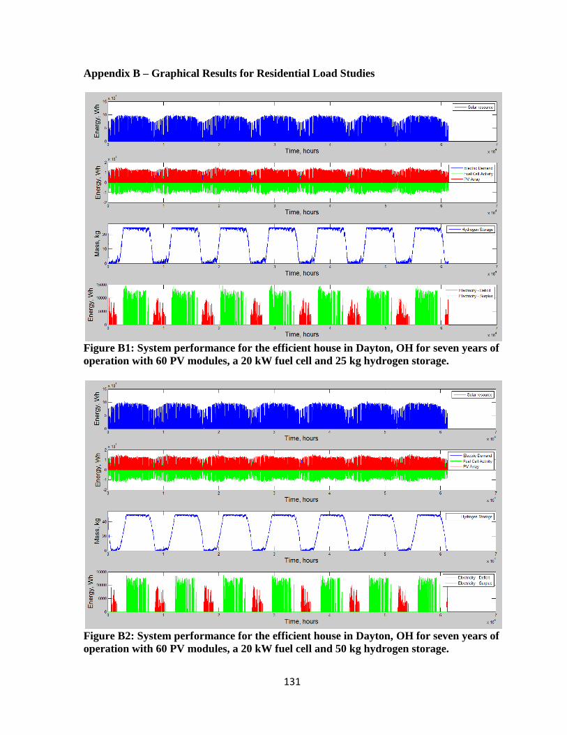
131

Appendix B – Graphical Results for Residential Load Studies


operation with 60 PV modules, a 20 kW fuel cell and 25 kg hydrogen storage.



132





Documents

A Computational Approach to Simulating the Performance of