Embed Size (px)
Citation preview
A Comprehensive Scaling Up Technique for
Pneumatic Transport Systems
By
Chandana Ratnayake
Department of Technology
Telemark University College (HiT-TF)
Kjølnes Ring, N-3914 Porsgrunn
Norway
Thesis submitted to
The Norwegian University of Sceince and Technology (NTNU)
for the degree of Dr. Ing.
Porsgrunn, September 2005
i
ABSTRACT
The main objective of this investigation was to formulate a comprehensive scaling up
technique for designing of pneumatic conveying systems by addressing the whole
pipeline together with all accessories.
Five different bulk materials together with five qualities of one of these materials
have been used for the tests. A large number of pneumatic conveying tests has been
conducted for five different pipeline configurations.
In order to develop a model for pressure drop prediction in different sections of
pipeline i.e., horizontal, vertical, bends, valves, etc, the gas-solid flow has been
considered to be a mixture having its own flow characteristics. The classical Darcy-
Weisbach’s equation has been suitably modified and used for prediction of pressure
drop of gas-solid mixture. The concept of suspension density and pressure drop
coefficient has been introduced. Two separate models for pressure drop
determination have been proposed. While one is used for both horizontal and vertical
straight pipe sections, other is used for bends, valves or any other pipe section, which
are considered as individual units. It has been shown that the proposed model
performs much better than other scaling up techniques considered under the present
study.
Using dimensional analysis, a model has been formulated to scale up the pressure
drop incurred at the entry section of a top discharge blow tank. The proposed model
predicts the entry pressure losses within a maximum error margin of ±15% of
experimental measurements. Since no other model was found in the open literature
for such prediction, the proposed model could not be compared with any other.
To determine the minimum conveying velocity, a scaling up model has been
proposed using multivariate data analysis techniques and dimensional analysis. The
proposed model gives resoably better predictions, especially in case of fine particles,
than the other available models considered in this study. It also shows a good
agreement with experimental measurements.

ii
Combining the models proposed in current study for pressure drop determination,
entry loss calculation and minimum conveying velocity estimation, one can reliably
design a complete pneumatic conveying system.
Computational fluid dynamics (CFD) principles have been used to determine the
pressure drop across a standard 90º bend and a straight pipe section. A commercial
software code; Fluent® has been used for the investigation. Eulerian approach has
been used for the simulation and the results show that the tested software can be used
as an effective tool to determine the pressure drop in pneumatic conveying systems.
iii
ACKNOWLEDGEMENT
The experimental investigation described in this thesis has become a reality with the
help of many individuals and organisations. Although it is a hard task to list each and
every one of them, the author is struggling here to acknowledge their support for
carrying out this scientific study being a foreign student in Norway.
• Firstly, I would like to express my sincere gratitude to Dr. Biplab K. Datta
and Prof. Morten C. Melaaen for their invaluable guidance, encouragement
and interesting discussions through out the work, amidst their busy schedules.
• I am greatly indebted to late Prof. Sunil D. Silva who helped me to come to
Norway as a graduate student. Even though, I unfortunately missed him in
early stage of this study, his inspiration for such a comprehensive work is
greatly acknowledged.
• All my colleagues in POSTEC group are highly appreciated for their
technical support for the research study as well as their social support, which
has made my stay in Norway enjoyable.
• Many thanks also go all staff members of Telemark University College,
specially, Unni S. Kassin, Trine Ellefsen, Anne Solberg, Inger Kristiansen,
Anne M. Blichfeldt, Marit Olsen, Jarle Teigen and Inger-Judith for their
kindly help.
• All administrative staff of Telemark Technological Research and
Development Centre (Tel-Tek), specially, Marit Larsen, Liv Axelsen, June
Kvasnes and Anniken Augestad are commended for their support.
• The Norwegian state education loan fund (Lånekassen), Tel-Tek,
MODPOWFLOW scheme funded by The Norwegian Research Council
(NFR) and POSTEC members are acknowledged for their financial support.
• I acknowledge my gratitude tawards National Oilwell, Statoil, Hydro
aluminium and Unitor ASA for permitting publication of the findings of the
studies, funded by them.

iv
• Finally, I express my heartiest appreciation to my beloved wife; Chamila and
two kids; Kavindu and Kaveesha for their patience and moral support during
this work. Very special thanks to my mother and two sisters for their
continuous encouragement and moral support extended to me from my
country Sri Lanka.
September, 2005 Chandana Ratnayake
v
CONTENT
Abstract ......................................................................................................... i
Acknowledgement ...................................................................................... iii
Content ......................................................................................................... v
Nomenclature............................................................................................. xii
1 Introduction............................................................................................. 1
1.1 Introduction of Pneumatics and its Applications .............................. 1
1.2 Definition of Pneumatic Conveying.................................................. 1
1.3 History of Pneumatic Conveying...................................................... 2
1.4 Applications of Pneumatic Conveying.............................................. 4
1.5 Advantages and Limitations of Pneumatic Conveying..................... 6
1.6 Major Components in a Typical Pneumatic Conveying System....... 7
1.7 Classification of Pneumatic Conveying Systems ............................. 7
1.8 Operation of a Pneumatic Conveying System ............................... 11
1.8.1 Horizontal Conveying ..........................................................................12
1.8.2 Vertical Conveying...............................................................................14
1.9 Motivation ...................................................................................... 15
1.10 Aim of the Project .......................................................................... 18
1.11 Outline of the Thesis...................................................................... 18
2 Background and review of literature .................................................. 21
2.1 Introduction.................................................................................... 21
2.2 Entry section.................................................................................. 22
2.3 Blow Tank...................................................................................... 23
2.3.1 Top Discharge and Bottom Discharge .................................................23
2.3.2 Velocity at Entry Section......................................................................24
2.4 Horizontal Pipe Sections................................................................ 24
2.4.1 Pressure Drop Determination ..............................................................25
2.4.1.1 ‘Air-Only’ Pressure Drop ..............................................................262.4.1.2 Pressure Drop Due to Solid Particles...........................................272.4.1.3 Solid Friction Factor.....................................................................29
2.4.2 Acceleration Length and Pressure Drop ..............................................34
vi
2.4.3 Dense Phase Transport.......................................................................36
2.5 Vertical Pipe Sections.................................................................... 43
2.6 Inclined Pipe Sections ................................................................... 45
2.7 Pipe Bends .................................................................................... 46
2.8 Velocity Consideration................................................................... 49
2.8.1 Determination of Minimum Conveying Velocity....................................50
2.8.2 Choking Velocity in Vertical Flows .......................................................54
2.8.3 Determination of Average Particle Velocity..........................................55
2.9 Scale Up Techniques..................................................................... 57
2.9.1 Mills Scaling Technique.......................................................................57
2.9.1.1 Straight Horizontal Pipe Section ..................................................582.9.1.2 Effect of Bends ............................................................................582.9.1.3 Total Length.................................................................................582.9.1.4 Pipe Diameter..............................................................................59
2.9.2 Wypych & Arnold Scaling Method........................................................59
2.9.3 Keys and Chambers Scaling Technique ..............................................60
2.9.4 Molerus Scaling Technique .................................................................61
2.9.5 Bradley et al. Scaling Technique .........................................................61
2.10 Effects of Material Physical Characteristics ................................... 62
2.11 Computational Models ................................................................... 66
2.11.1 Applications of CFD in Gas-Solid Flows...........................................68
2.11.2 CFD Applications in Pneumatic Conveying......................................70
3 Experimental Setup and Instrumentations......................................... 72
3.1 Available Pneumatic Transport Test Facilities at POSTEC Powder
Hall ……………………………………………………………………………72
3.2 Air Compressor.............................................................................. 73
3.3 Dryer cum Cooler .......................................................................... 74
3.4 Control Valves ............................................................................... 74
3.5 Control Room ................................................................................ 76
3.6 Pressure Transducers ................................................................... 77
3.7 Air Flow Meter ............................................................................... 79
3.8 Weigh Cells ................................................................................... 79
3.9 Temperature and Humidity Transmitter ......................................... 80
vii
3.10 Blow Tank...................................................................................... 80
3.11 Pipelines ........................................................................................ 82
3.12 Data Acquisition and Processing ................................................... 83
3.13 Particle Size Analyser.................................................................... 86
4 Pressure Drop determination and Scale up Technique .................... 87
4.1 Introduction.................................................................................... 87
4.2 Theoretical Approach..................................................................... 89
4.2.1 Background .........................................................................................89
4.2.2 Formulation of New Model...................................................................91
4.3 Material Data ................................................................................. 92
4.3.1 Barytes ................................................................................................92
4.3.2 Bentonite .............................................................................................93
4.3.3 Cement................................................................................................93
4.3.4 Ilmenite................................................................................................94
4.3.5 Alumina ...............................................................................................94
4.4 Experimental Set-up ...................................................................... 97
4.5 Experimental Procedure ................................................................ 99
4.6 Experimental Results................................................................... 102
4.6.1 Pneumatic Conveying Characteristics Curves ...................................102
4.6.2 Loading and Conveying Velocities.....................................................106
4.7 Variations of ‘K’ Curves ............................................................... 107
4.7.1 Method of ‘K’ Calculation ...................................................................107
4.7.2 ‘K’ vs. V2entry Curves ...........................................................................109
4.7.2.1 Straight Pipe Sections (Horizontal and Vertical).........................1104.7.2.2 Bends and Valves......................................................................115
4.7.3 The Effect of Particle Size on ‘K’........................................................116
4.7.3.1 Horizontal Pipe Sections............................................................1174.7.3.2 Vertical pipe Section ..................................................................118
4.7.4 Summary of Findings.........................................................................118
4.8 Model Validation .......................................................................... 119
4.8.1 Calculation Procedure of Validation...................................................119
4.8.2 Validation Results..............................................................................121
4.8.2.1 Graphical Comparison ...............................................................1224.8.2.2 Analytical Comparison ...............................................................123
4.9 Summary ..................................................................................... 127
viii
5 Comparison Analysis of ‘K’ factor Method with other Models ....... 128
5.1 Introduction.................................................................................. 128
5.2 Outline of Scaling Techniques ..................................................... 129
5.3 Method of Comparison ................................................................ 130
5.4 Test Setup and Conveying Materials ........................................... 130
5.5 Calculation Procedure ................................................................. 131
5.6 Results and Discussion ............................................................... 132
5.6.1 Piecewise Consideration ...................................................................133
5.6.1.1 Graphical Comparison ...............................................................1335.6.1.2 Analytical Comparison ...............................................................138
5.6.2 Whole Conveying Line Consideration................................................141
5.6.2.1 Graphical Comparison ...............................................................1415.6.2.2 Analytical Comparison ...............................................................144
5.7 Conclusion................................................................................... 145
6 Prediction of pressure drop at the entry section of top discharge
blow tank…………………………… ........................................................... 147
6.1 Introduction.................................................................................. 147
6.2 Background ................................................................................. 147
6.3 Test Setup ................................................................................... 148
6.4 Details of Experiments................................................................. 150
6.5 Theoretical Approach................................................................... 150
6.5.1 List of influential parameter................................................................151
6.5.2 Number of Dimensionless Groups Required......................................151
6.5.3 Determination of Repeating Variables ...............................................152
6.5.4 Formation of Dimensionless Groups..................................................153
6.5.4.1 A Specimen Simplification .........................................................1536.5.5 Final Form of Functional Relationship................................................154
6.6 Model Formulation....................................................................... 155
6.7 Validation of Model ...................................................................... 159
6.7.1 Graphical Comparison.......................................................................160
6.7.2 Analytical Comparison.......................................................................162
6.8 Conclusion................................................................................... 164
7 Scaling up of Minimum Conveying Conditions in a Pneumatic
Transport System………………… ........................................................... 165
ix
7.1 Introduction.................................................................................. 165
7.2 Background ................................................................................. 166
7.2.1 Rizk method [38, 176]........................................................................167
7.2.2 Hilgraf method [175, 182, 183]...........................................................167
7.2.3 Wypych method [174]........................................................................168
7.2.4 Matsumoto method [37] .....................................................................168
7.2.5 Doig & Roper method [169] ...............................................................168
7.2.6 Martinussen’s model [36]...................................................................169
7.3 Test Setup and Material............................................................... 169
7.4 Theoretical Consideration............................................................ 169
7.4.1 The Influential Variables ....................................................................170
7.4.2 Use of Multivariate Data Analysis ......................................................171
7.4.3 Data Analysis Trials...........................................................................172
7.4.3.1 PCA...........................................................................................1727.4.3.2 PLS Regression.........................................................................174
7.4.4 Determination of Dimensionless Groups............................................175
7.5 Test Results................................................................................. 176
7.6 Model Verification with Experimental Results .............................. 177
7.7 Validation..................................................................................... 180
7.8 Comparison with Others Models.................................................. 182
7.9 Prediction of Minimum Conveying Boundary in Experimental PCC…
…………………………………………………………………………..185
7.10 Conclusion................................................................................... 188
8 Putting It All Together and a Case Study ......................................... 189
8.1 Introduction.................................................................................. 189
8.2 General Calculation Programme ................................................. 190
8.2.1 Implementation of Model Relationships .............................................190
8.2.2 Introduction of Design Input...............................................................191
8.2.2.1 Main Inputs ................................................................................1928.2.2.2 Material Data .............................................................................1928.2.2.3 Geometrical Parameters ............................................................192
8.2.3 Pressure Drop and Velocity Calculation.............................................193
8.2.4 Presentation of Output Results ..........................................................194
8.3 Use of Calculation Programme.................................................... 195
x
8.4 An Application: A Case Study...................................................... 196
8.4.1 Background .......................................................................................196
8.4.2 Experimental Test Set-up ..................................................................196
8.4.3 Usage of the Calculation Programme ................................................199
8.5 Conclusion................................................................................... 201
9 Computational Fluid Dynamics as a Pressure Drop Prediction Tool
in Dense Phase Pneumatic Conveying Systems .................................. 202
9.1 Introduction.................................................................................. 202
9.2 Background ................................................................................. 203
9.3 Test Sections............................................................................... 204
9.4 Theoretical Consideration............................................................ 205
9.4.1 CFD Model ........................................................................................206
9.4.2 Model Equations................................................................................207
9.4.2.1 Continuity equations ..................................................................2079.4.2.2 Momentum equations ................................................................2079.4.2.3 Solids phase pressure ...............................................................2089.4.2.4 Gas-solid particle exchange coefficient ......................................2089.4.2.5 Solids Viscosity..........................................................................2099.4.2.6 Turbulent kinetic energy equation ..............................................2109.4.2.7 Granular Temperature Equation ................................................213
9.5 Grid Generation ........................................................................... 214
9.5.1 Bend..................................................................................................214
9.5.2 Straight Section .................................................................................215
9.6 Numerical Simulation................................................................... 217
9.7 Results and Discussion ............................................................... 219
9.7.1 Variation of Volume Fraction .............................................................220
9.7.1.1 Bend ..........................................................................................2209.7.1.2 Straight Section .........................................................................222
9.7.2 Velocity profiles of gas and solid phase.............................................223
9.7.3 Pressure drop determination .............................................................227
9.8 Conclusion................................................................................... 230
10 Conclusions and Suggestions for Future Work .............................. 231
10.1 Introduction.................................................................................. 231
10.2 General Conclusions ................................................................... 231
10.2.1 Scaling up of Line Pressure Drop ..................................................232
xi
10.2.2 Scaling up of Entry Loss ................................................................234
10.2.3 Scaling up of Minimum Conveying Velocity ...................................234
10.2.4 Computer Based Calculation Programme......................................234
10.2.5 CFD Simulation on Pipe Bends and Straight Sections ...................235
10.3 Suggestion for Future Works ....................................................... 236
11 Bibliography........................................................................................ 238
12 Appendices ......................................................................................... 258
���� Particle Size Distributions ................................................................. 258
���� Pneumatic conveying characteristics curves .................................. 263
���� Validation Curves ............................................................................... 270
���� List of Publications ............................................................................ 276

xii
NOMENCLATURE
A pipe cross-sectional area [m2]
b bend equivalent length [m]
B bend pressure loss coefficient [-]
C constant [-]
Cμ turbulence model constant (given in Table 9-2) [-]
CD drag coefficient [-]
Ci (i:1…n) constants [-]
Ciε (i:1,2,3) turbulence model constant (given in Table 9-2) [-]
Cmk ratio between solids and air velocities [-]
D diameter [m]
dp particle diameter [m]
ess coefficient of restitution [-]
Eu Euler number [-]
f friction factor [-]
Fr Froude number [-]
Frst Froude number related to starting velocity [-]
g acceleration of gravity [m/s2]
G rate of production of turbulent kinetic energy [-]
g0,ss radial distribution function [as given in Equation (9.8)] [-]
K pressure drop coefficient [as introduced in Equation (4.5)] [-]
k turbulent kinetic energy [m2/s2]
kb bend pressure loss coefficient [-]
Ki,j inter-phase momentum exchange coefficient (from i to j) [-]
kw coefficient of internal wall friction [-]
L length of pipe section [m]
Lb length of the bend [m]
lp length of the plug [m]
xiii
Ls length of solid column [i.e., (total volume of moving
solids)/ (tube area)] [m]
m mass flow rate [kg/s]
M molecular weight [-]
p pressure [N/m2]
P local pressure [N/m2]
R, r radius [m]
Re Reynolds number [-]
T absolute temperature [K]
U superficial velocity [m/s]
Uf actual fluid velocity [m/s]
ui velocity of i phase [m/s]
Ut particle terminal velocity of a single particle [m/s]
v velocity [m/s]
V volumetric flow rate [m3/s]
vst starting velocity [m/s]
ws slip velocity [m/s]
xi (i:1…n) constant [-]
Greek Symbols
αi volume fraction of i phase [-]
β0 coefficient of wall friction [-]
δij Kroenecker delta [-]
Δp pressure drop [N/m2]
ε pipe roughness [m]
εs volume fraction of solid [-]
ζ additional pressure loss factor [-]
η dimensionless number [as introduced in Equation (6.22)] [-]
θ angle of inclination of the pipe [deg.]
θs granular temperature [m2/s2]
xiv
λ friction factor [-]
μ solids loading ratio [-]
μd dynamic viscosity [kg/ms]
μeff,g effective viscosity of gas [kg/ms]
μi viscosity of phase i [kg/ms]
μt turbulent viscosity [kg/ms]
μw tan φw [-]
�i dimensionless number [-]
ρ density [kg/m3]
� standard deviation [-]
σf normal stress at front face of slug [N/m2]
σi,j turbulence model constant (given in Table 9-2) [-]
υs solids bulk viscosity [kg/ms]
τij,g stress tensor gas phase [kg/ms2]
φw angle of wall friction [deg.]
Ψs shape factor [-]
Subscripts
a parameter due to air
A parameters relevant acceleration pressure drop
b bend
c choking condition
cal calculated value
col collisional
e error
entry entry conditions
eq equivalent
exp experimentally measured value
g gas phase

xv
h horizontal
i inlet section conditions
kin kinetic
m mean value
max maximum
min minimum
o outlet section condition
s solid phase
st straight pipe section
start condition at starting of pipeline
sus suspension
t parameter for total flow
T parameters relevant particles terminal velocity
v vertical
1
1 INTRODUCTION
1.1 Introduction of Pneumatics and its Applications
Being originated from a Greek word ‘pneumatikos’, which means coming from the
wind, pneumatics means the use of pressurized air in science and technology. Its
applications can be seen in various industries and domestic appliances as well.
Easiness in controlling and flexibility in installations are some of the favourable
features of pneumatics applications in many industrial and non-industrial fields.
Pneumatic conveying of particulate material is another well known application of
pneumatics in the field of handling of particulate materials. This chapter looks into
the details of history, advantages, disadvantages and basic types of pneumatic
conveying systems. The motivation of this experimental investigation is described in
detail in a later section. An outline of the thesis structure is also provided at the end
of this Chapter.
1.2 Definition of Pneumatic Conveying
Pneumatic conveying is a material transportation process, in which bulk particulate
materials are moved over horizontal and vertical distances within a piping system
with the help of a compressed air stream. Using either positive or negative pressure
of air or other gases, the material to be transported is forced through pipes and finally
separated from the carrier gas and deposited at the desired destination. A general
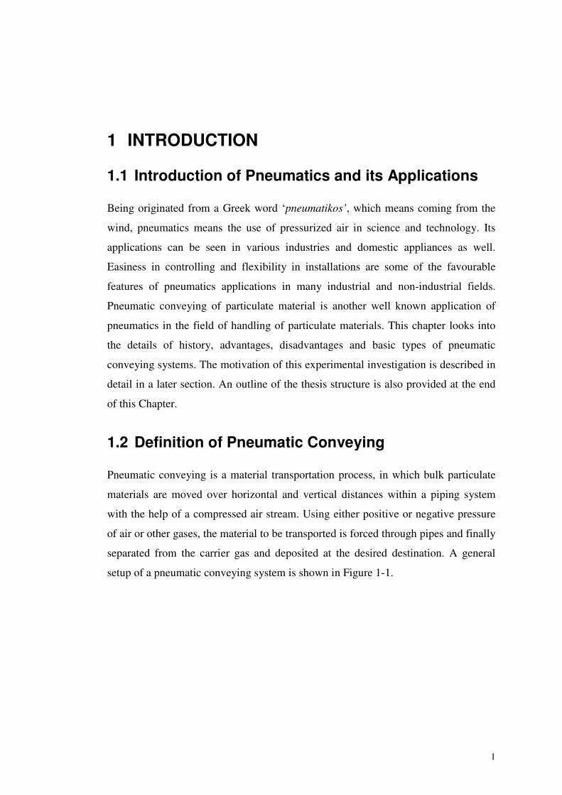
setup of a pneumatic conveying system is shown in Figure 1-1.
2
Figure 1-1: General setup of a pneumatic conveying plant [1].
This mode of bulk solid transportation holds an important position in the particulate
material handling field, because of a series of advantages over other modes of
transportation. It has a wide range of applications, with examples ranging from
domestic vacuum cleaners to the transport of some powder materials over several
kilometres. With a recorded history of more than a century, pneumatic conveying
systems have been popularised in the bulk material handling field.
1.3 History of Pneumatic Conveying
Pneumatic tubes used for transporting physical objects have a long history. The basic
principles of pneumatics were stated by the Greek Hero of Alexandria before 100 BC
[2].�On the other hand, the concept of conveying materials in pipeline systems also
goes back to pre-historical age with some evidence of that the Romans used lead
pipes for water supply and sewage disposal and the Chinese used bamboo to convey
natural gas [3].
Although there had been various applications of pneumatic conveying earlier in
many civilisations, the first documented pipeline conveying of solid particles was
3
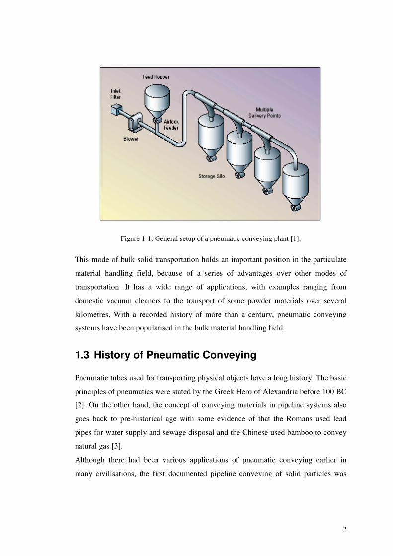
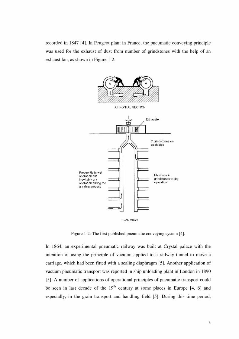
recorded in 1847 [4]. In Peugeot plant in France, the pneumatic conveying principle
was used for the exhaust of dust from number of grindstones with the help of an
exhaust fan, as shown in Figure 1-2.
Figure 1-2: The first published pneumatic conveying system [4].
In 1864, an experimental pneumatic railway was built at Crystal palace with the
intention of using the principle of vacuum applied to a railway tunnel to move a
carriage, which had been fitted with a sealing diaphragm [5]. Another application of
vacuum pneumatic transport was reported in ship unloading plant in London in 1890
[5]. A number of applications of operational principles of pneumatic transport could
be seen in last decade of the 19th century at some places in Europe [4, 6] and
especially, in the grain transport and handling field [5]. During this time period,
4
general break through events in the evolution of pneumatic conveying systems such
as use of negative pressure systems, invention of auxiliary equipments like rotary
feeders, screw feeders, valves, etc., could be emphasised.
During early decades of 20th century, it was common practice to use pneumatic
conveying to transport grain [6]. Ref. [7] presented a chronology of pneumatic
pipeline highlighting the innovatory individuals and companies, especially during
early and middle era of 20th century. During the First World War, the development of
pneumatic conveying was influenced by the high demand for foods, labour
scarceness and risks of explosion. Since the pneumatic conveying systems were seen
as the answer for those situations, a huge evolution of pneumatic transport was
achieved during that time period. In the post-war period, pneumatic conveying
systems were used for more industrial related materials like coal and cement.
Beginning of theoretical approaches, invention of blowers, introduction of batch
conveying blow tanks, etc., were among the highlighted milestones of the evolution
of pneumatic transport systems during this era.
Nowadays, pneumatic transport is a popular technique in particulate material
handling field. It has been reported that some plants have transport distance of more
than 40 km [8], material flow rate of few hundreds tons per hour and solid loading
ratio (the mass flow rate ratio between solid and air ) of more than 500.
1.4 Applications of Pneumatic Conveying
The applications of pneumatic conveying systems can be seen in many industrial
sectors. A list of industrial fields where it has extensively been used is given below;
• Chemical process industry
• Pharmaceutical industry
• Mining industry
• Agricultural industry
• Mineral industry
• Food processing industry
5
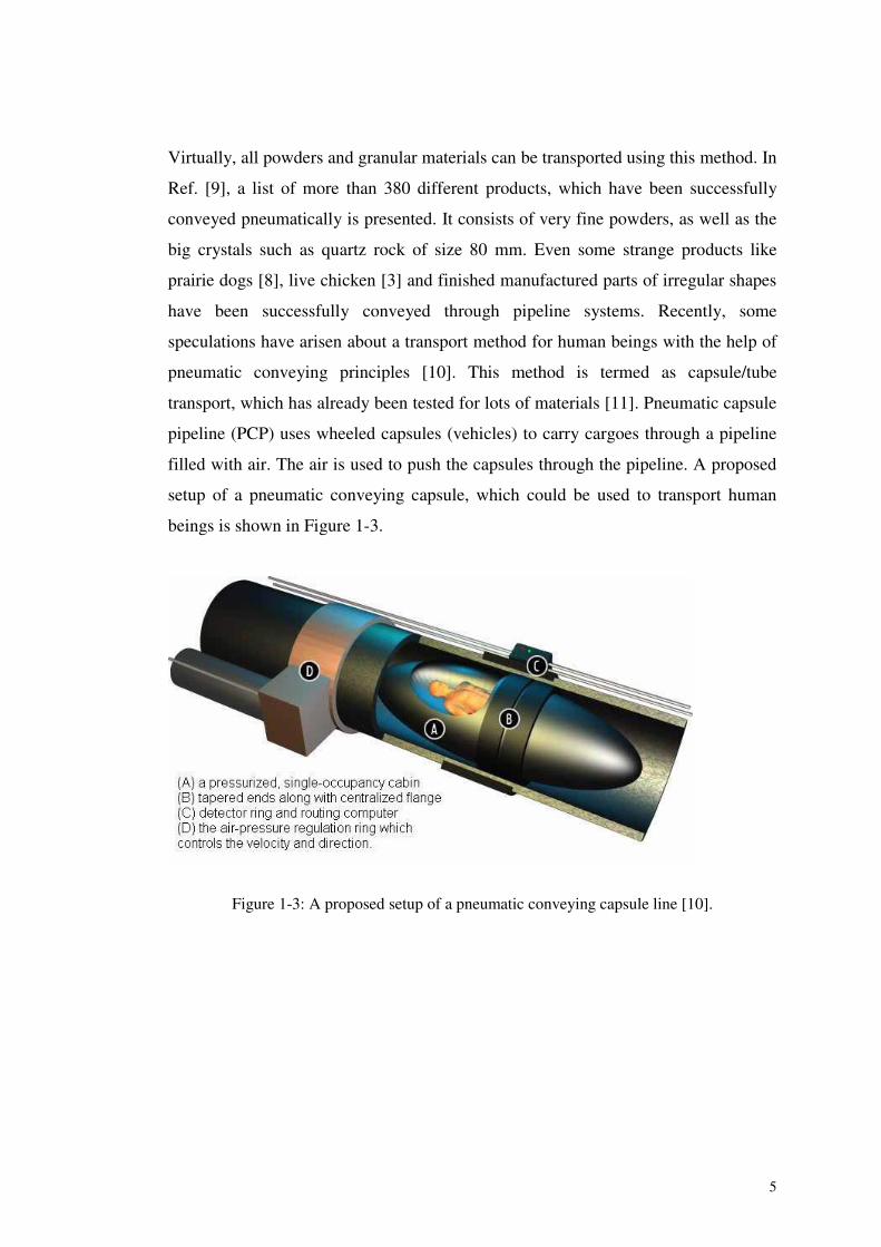
Virtually, all powders and granular materials can be transported using this method. In
Ref. [9], a list of more than 380 different products, which have been successfully
conveyed pneumatically is presented. It consists of very fine powders, as well as the
big crystals such as quartz rock of size 80 mm. Even some strange products like
prairie dogs [8], live chicken [3] and finished manufactured parts of irregular shapes
have been successfully conveyed through pipeline systems. Recently, some
speculations have arisen about a transport method for human beings with the help of
pneumatic conveying principles [10]. This method is termed as capsule/tube
transport, which has already been tested for lots of materials [11]. Pneumatic capsule
pipeline (PCP) uses wheeled capsules (vehicles) to carry cargoes through a pipeline
filled with air. The air is used to push the capsules through the pipeline. A proposed
setup of a pneumatic conveying capsule, which could be used to transport human
beings is shown in Figure 1-3.
Figure 1-3: A proposed setup of a pneumatic conveying capsule line [10].
6
1.5 Advantages and Limitations of Pneumatic
Conveying
In recent years, pneumatic transport systems are being used much more often,
acquiring market sectors, in which other types of transport were typically used,
especially in the field of bulk solids handling and processing. The reason is a series
of advantages it has over the other methods of material conveying such as
mechanical conveyers. Because of the flexibility of installation, this mode of bulk
solids conveying is specially used to deliver dry, granular or powdered materials via
pipelines to remote plant areas that would be hard to reach economically with
mechanical conveyers. Since pneumatic systems are completely enclosed, product
contamination, material loss and dust emission (thus, environment pollution) are
reduced or eliminated. Particularly, to convey materials hazardous to health, a
negative pressure (vacuum) pneumatic system is the best option. On the other hand,
pneumatic conveying systems can be adopted to pick up the conveying bulk material
from multiple sources and/or distribute them to many different destinations. In
addition, reduced dimensions, progressive reduction of capital and installation costs,
low maintenance costs (due to the small number of moving parts), repeated usage of
conveying pipelines, easiness in control and automation are among the favourable
advantages of pneumatic conveying over the other traditional methods of particulate
material handling.
Although pneumatic conveying has seen increased use in many industrial sectors,
there are still many major problems hampering its employment in a wider range of
industrial conveying applications. Specially, in dilute-phase transport, high energy
consumption, excessive product degradation and system erosion (pipelines, bends
etc) are some of the major problems. In an alternative method, in dense-phase
conveying also, unstable plugging phenomena, severe pipe vibration and repeated
blockages are experienced frequently. Further, the lack of simple procedures for the
selection of an optimal system is a major problem in pneumatic transport system
design.
7
1.6 Major Components in a Typical Pneumatic
Conveying System
There are a number of components in a pneumatic conveying plant, which are
required to achieve the particular duty condition. Usually, a typical conveying system
comprises different zones where distinct operations are carried out. In each of these
zones, some specialised equipments are required for the successful operation of the
plant. Any pneumatic conveying system usually consists of four major components;
1. Conveying gas supply-
To provide the necessary energy to the conveying gas, various types of
compressors, fans, blowers and vacuum pumps are used as the prime mover.
2. Feeding mechanism-
To feed the solid to the conveying line, a feeding mechanism such as rotary
valve, screw feeder, etc, is used.
3. Conveying line-
This consists of all straight pipe lines of horizontal and/or vertical sections,
bends and other auxiliary components such as valves.
4. Separation equipment-
At the end of the conveying line, solid has to be separated from the gas
stream in which it has been transported. For this purpose, cyclones, bag
filters, electrostatic precipitators are usually used in the separation zone.
1.7 Classification of Pneumatic Conveying Systems
Pneumatic transport systems can be classified in a number of ways. Among them, the
nature of system pressure and the mode of conveying are the two major aspects for
the classification. So far as the system pressure is concerned, there are three major
types of transport systems, which can briefly be explained in the following way:-
1. Positive pressure systems –
In this type of pneumatic conveying system, the absolute pressure of
conveying gas inside the piping system is always greater than atmospheric
8
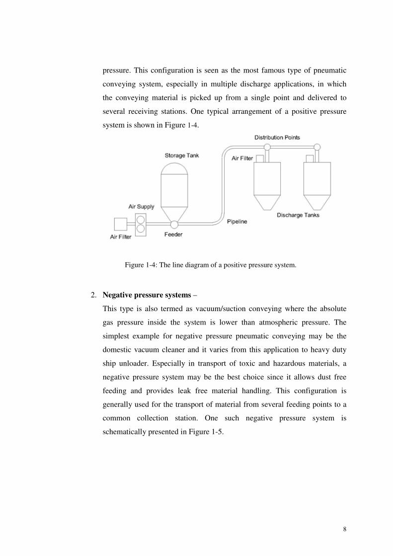
pressure. This configuration is seen as the most famous type of pneumatic
conveying system, especially in multiple discharge applications, in which
the conveying material is picked up from a single point and delivered to
several receiving stations. One typical arrangement of a positive pressure
system is shown in Figure 1-4.
Figure 1-4: The line diagram of a positive pressure system.
2. Negative pressure systems –
This type is also termed as vacuum/suction conveying where the absolute
gas pressure inside the system is lower than atmospheric pressure. The
simplest example for negative pressure pneumatic conveying may be the
domestic vacuum cleaner and it varies from this application to heavy duty
ship unloader. Especially in transport of toxic and hazardous materials, a
negative pressure system may be the best choice since it allows dust free
feeding and provides leak free material handling. This configuration is
generally used for the transport of material from several feeding points to a
common collection station. One such negative pressure system is
schematically presented in Figure 1-5.
9
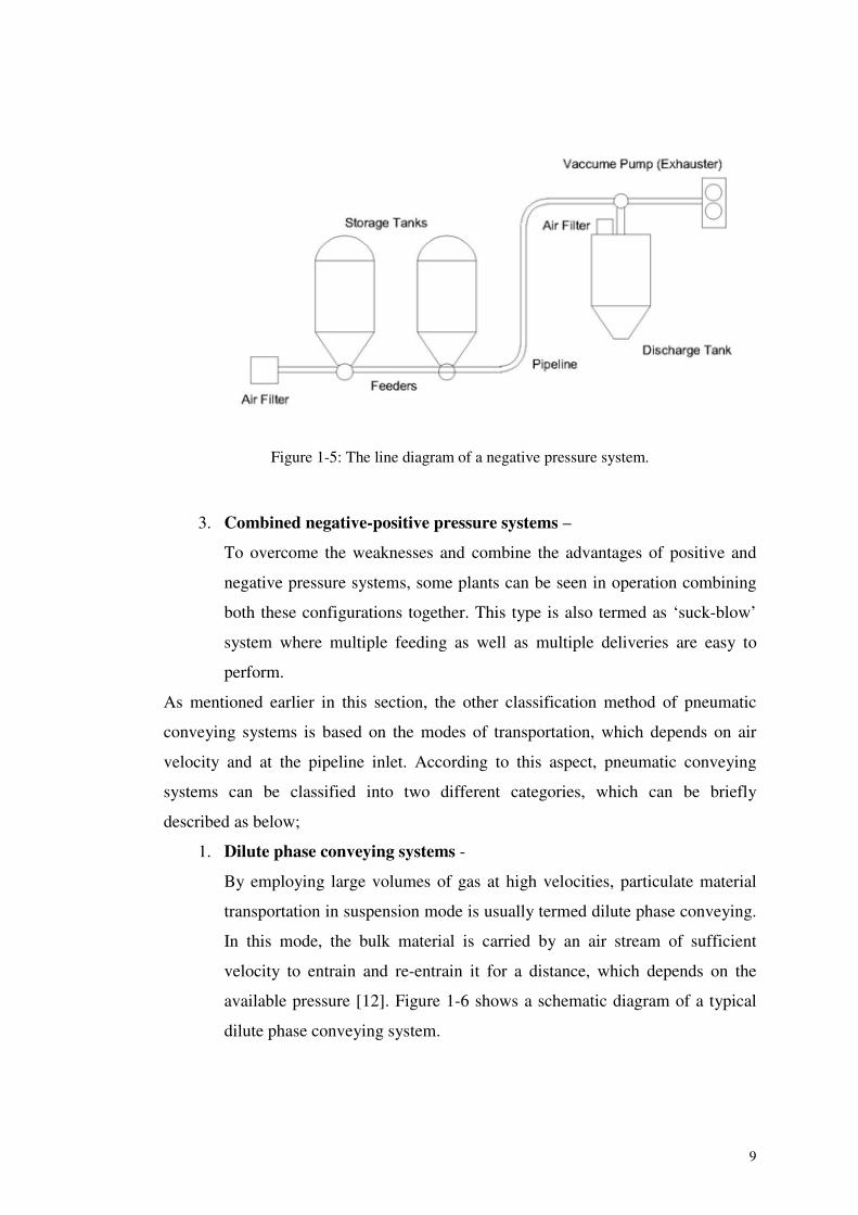
Figure 1-5: The line diagram of a negative pressure system.
3. Combined negative-positive pressure systems –
To overcome the weaknesses and combine the advantages of positive and
negative pressure systems, some plants can be seen in operation combining
both these configurations together. This type is also termed as ‘suck-blow’
system where multiple feeding as well as multiple deliveries are easy to
perform.
As mentioned earlier in this section, the other classification method of pneumatic
conveying systems is based on the modes of transportation, which depends on air
velocity and at the pipeline inlet. According to this aspect, pneumatic conveying
systems can be classified into two different categories, which can be briefly
described as below;
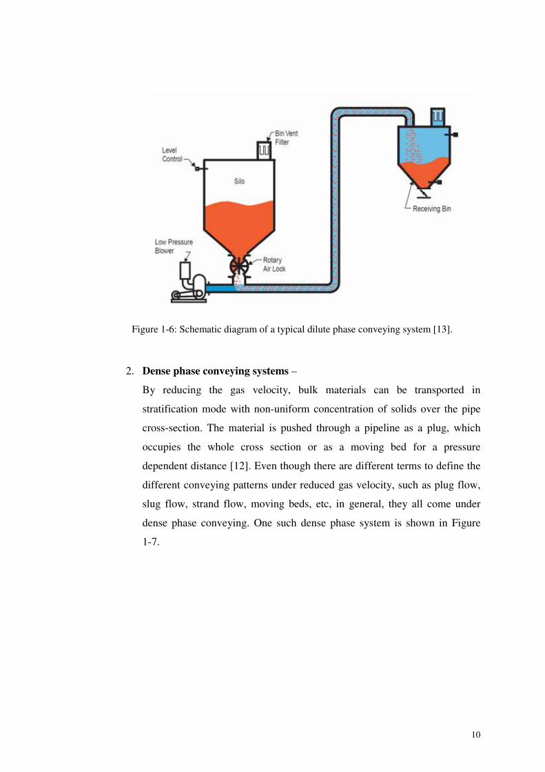
1. Dilute phase conveying systems -
By employing large volumes of gas at high velocities, particulate material
transportation in suspension mode is usually termed dilute phase conveying.
In this mode, the bulk material is carried by an air stream of sufficient
velocity to entrain and re-entrain it for a distance, which depends on the
available pressure [12]. Figure 1-6 shows a schematic diagram of a typical
dilute phase conveying system.
10
Figure 1-6: Schematic diagram of a typical dilute phase conveying system [13].
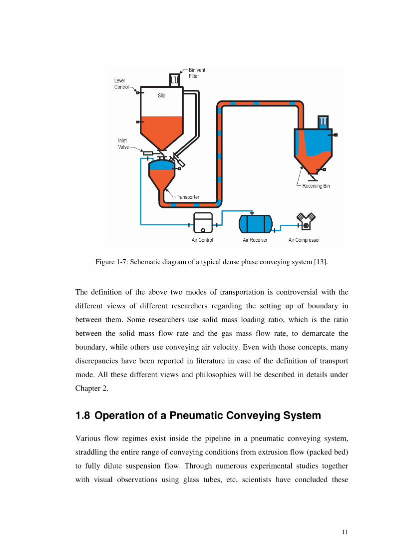
2. Dense phase conveying systems –
By reducing the gas velocity, bulk materials can be transported in
stratification mode with non-uniform concentration of solids over the pipe
cross-section. The material is pushed through a pipeline as a plug, which
occupies the whole cross section or as a moving bed for a pressure
dependent distance [12]. Even though there are different terms to define the
different conveying patterns under reduced gas velocity, such as plug flow,
slug flow, strand flow, moving beds, etc, in general, they all come under
dense phase conveying. One such dense phase system is shown in Figure
1-7.
11
Figure 1-7: Schematic diagram of a typical dense phase conveying system [13].
The definition of the above two modes of transportation is controversial with the
different views of different researchers regarding the setting up of boundary in
between them. Some researchers use solid mass loading ratio, which is the ratio
between the solid mass flow rate and the gas mass flow rate, to demarcate the
boundary, while others use conveying air velocity. Even with those concepts, many
discrepancies have been reported in literature in case of the definition of transport
mode. All these different views and philosophies will be described in details under
Chapter 2.
1.8 Operation of a Pneumatic Conveying System
Various flow regimes exist inside the pipeline in a pneumatic conveying system,
straddling the entire range of conveying conditions from extrusion flow (packed bed)
to fully dilute suspension flow. Through numerous experimental studies together
with visual observations using glass tubes, etc, scientists have concluded these
12
varieties of flow regimes. It has been seen that these different flow regimes could be
explained easily in terms of variations of gas velocity, solids mass flow rate and
system pressure drop. This clarification also explains the general operation of a
pneumatic conveying system.
Most of the research workers and industrial system designers have used a special
graphical technique to explain the basic operation of a pneumatic conveying system.
This technique utilises the interaction of gas-solid experienced inside the conveying
pipeline in terms of gas velocity, solids mass flow rate and pressure gradient in pipe
sections in a way of graphical presentation, which was initially introduced by Zenz
[14, 15]. Some researchers [16-25] named this diagram as pneumatic conveying
characteristics curves, while others [6, 26-28] used the name of state or phase
diagram. The superficial air velocity and pressure gradient of the concerned pipe
section are usually selected as the x and y axes of the diagram and number of
different curves are produced on these set of axes in terms of different mass flow
rates of solids.
There is a distinguishable difference between the relevant flow regimes for
horizontal and vertical pipe sections. On the other hand, the particle size and particle
size distribution also have influence on the flow patterns inside the pipelines. The
general operation of horizontal and vertical pneumatic conveying systems are briefly
explained in the following sections with the help of pneumatic conveying phase
diagrams together with varieties of flow regimes.
1.8.1 Horizontal Conveying
One typical horizontal phase diagram is shown in Figure 1-8, together with various
cross-sectional diagrams showing the state of possible flow patterns at different flow
situations.
13
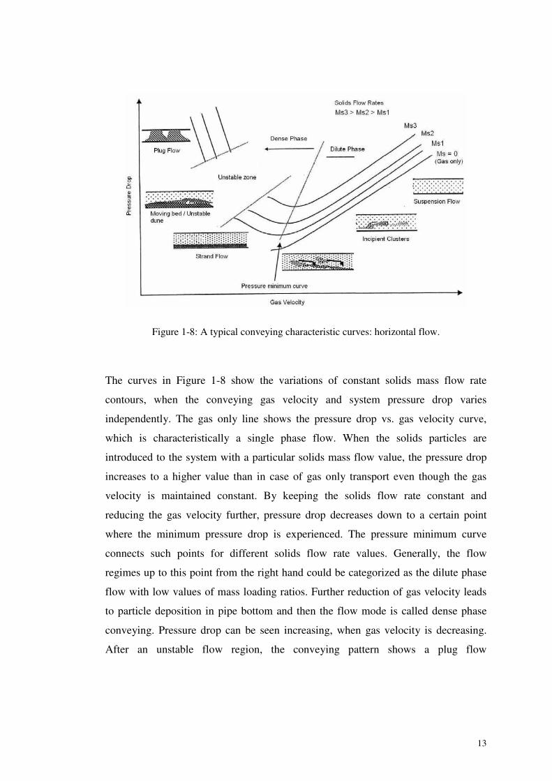
Figure 1-8: A typical conveying characteristic curves: horizontal flow.
The curves in Figure 1-8 show the variations of constant solids mass flow rate
contours, when the conveying gas velocity and system pressure drop varies
independently. The gas only line shows the pressure drop vs. gas velocity curve,
which is characteristically a single phase flow. When the solids particles are
introduced to the system with a particular solids mass flow value, the pressure drop
increases to a higher value than in case of gas only transport even though the gas
velocity is maintained constant. By keeping the solids flow rate constant and
reducing the gas velocity further, pressure drop decreases down to a certain point
where the minimum pressure drop is experienced. The pressure minimum curve
connects such points for different solids flow rate values. Generally, the flow
regimes up to this point from the right hand could be categorized as the dilute phase
flow with low values of mass loading ratios. Further reduction of gas velocity leads
to particle deposition in pipe bottom and then the flow mode is called dense phase
conveying. Pressure drop can be seen increasing, when gas velocity is decreasing.
After an unstable flow region, the conveying pattern shows a plug flow
14
characteristic, which will cause the pipeline to be totally blocked in attempts of
further reduction of gas velocity.
Figure 1-8 shows the different boundaries of the conveying characteristic curves.
One boundary is the extreme right hand side limitation, which depends on the air
volume flow capacity of the prime mover. The upper limit of the solid flow rate is
influenced by the allowable pressure value of compressed air supply. The left-hand
side boundary is fixed by the minimum conveying velocity, which will be discussed
in details in later chapter.
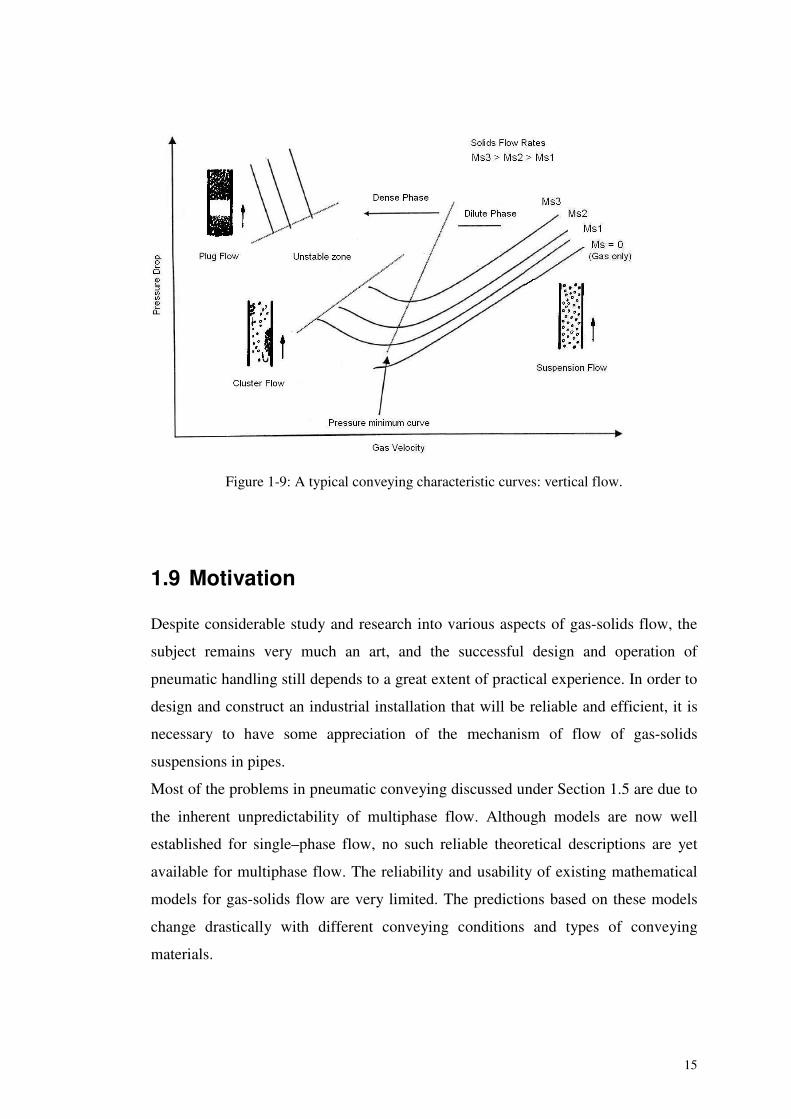
1.8.2 Vertical Conveying
The orientation of the pipe makes a considerable effect to the flow patterns and
conveying regimes, because of the influence of gravity force. Consequently, the
cross-sectional diagrams are totally different for the vertical pipe sections from those
of horizontal sections, although the general appearance of the mass flow rate
contours are similar to each other. Figure 1-9 shows a typical phase diagram of a
vertical pipe section, together with various cross-sectional diagrams showing the
representative state of possible flow patterns at different flow situations. Further
details of the vertical flow of pneumatic conveying will be discussed under Section
2.5.
15
Figure 1-9: A typical conveying characteristic curves: vertical flow.
1.9 Motivation
Despite considerable study and research into various aspects of gas-solids flow, the
subject remains very much an art, and the successful design and operation of
pneumatic handling still depends to a great extent of practical experience. In order to
design and construct an industrial installation that will be reliable and efficient, it is
necessary to have some appreciation of the mechanism of flow of gas-solids
suspensions in pipes.
Most of the problems in pneumatic conveying discussed under Section 1.5 are due to
the inherent unpredictability of multiphase flow. Although models are now well
established for single–phase flow, no such reliable theoretical descriptions are yet
available for multiphase flow. The reliability and usability of existing mathematical
models for gas-solids flow are very limited. The predictions based on these models
change drastically with different conveying conditions and types of conveying
materials.
16
To design a reliable pneumatic conveying system, basically two system parameters
should be established precisely. These are;
a) the pressure drop across the total pipeline system and
b) the minimum conveying condition for reliable transportation.
The total pressure drop is utilised to overcome the friction between the pipeline wall
and the gas-solids mixture, which can be considered as one of the flow properties of
the conveyed material. To prevent pipeline blockage, with minimum system power
consumption, the minimum conveying condition is employed. Since there are
numerous influential parameters (e.g. particle size and size distribution, particle
density, particle shape, etc.), empiricism has been used extensively, to establish the
mathematical models using some of the above parameters. Thus, the applicability of
these models to industry is very limited, and is reduced further for materials
possessing small particle size, relatively wide particle distributions, and complex
physical properties.
Therefore, designers are compelled to use experimentation in the design of industrial
pneumatic conveying installations. In this approach, a sample of product, which is to
be conveyed in the industrial plant, is tested in a laboratory pneumatic conveying test
rig (pilot plant) over a wide range of operating conditions. The product and airflow
rates and resulting pressure drops are measured as the test data. This approach has
the advantage that real test data on the product to be conveyed in the proposed
system are used for the design process. Thus, it gives a higher reliability level about
the effects of product type. This is very important because it provides useful
information on the conveyability of product and determination of minimum
conveying limits as well.
However, it is not always feasible to use a pilot plant, which is of identical geometry
(length, bore, number of bends, types of bends, etc.) to that of the required industrial
installation. Therefore, it is required to scale up the conveying characteristics that are
based on the pilot plant data, to predict the behaviour of the proposed industrial (full
scale) plant, using some experimentally determined factors. Scaling up in terms of
pipe line geometry needs to be carried out with respect to conveying distance,
pipeline bore, the air supply pressure available, etc. Pipeline material, bend geometry
17
and stepped pipelines are other important parameters that are also needed to be
considered.
The scaling up of pilot plant data is considered to be the most important stage of the
design process, because it provides the required link between laboratory pilot plant
test results and the full-scale industrial installation. Hence, accuracy and reliability of
scaling methodology are vital. A considerable number of researches have been
carried out to establish the mathematical models and relevant conditions of scaling
up procedure.
Several relationships, based on different conditions have been proposed in the
literature on scaling concepts, which will be discussed in details in Chapter 2.
Although these theories have been established with a number of investigations with
different materials and various pipeline configurations, there are still some doubts
and uncertainties about their validity, according to a recent experimental
investigation by the author [29]. The main objective of that investigation was to
examine the scale up criteria with regard to the transport distance and pipeline
diameter. As per the finding of the said investigation, it was clear that the predicted
values of pressure dropare over-estimated (higher than the experimental values), in
most of the cases. On the other hand, in case of scaling down, the available methods
do not also give correct results [29].
One popular alternative to the above explained classical methods of pressure drop
determination is the numerical simulation techniques using computational fluid
dynamic (CFD) principles. This technique has been very precise for the single phase
flow applications, but for multi phase flow situations like pneumatic transport it is
still to have a reliable prediction of flow patterns and determination of flow
parameter like pressure drop, solid velocity, etc. Recently, there has been a big
forward leap in CFD techniques with the invention of high speed computers and
innovative models to explain the flow phenomenon like turbulence, solid pressure
etc. The granular kinetic theory is a popular example for this kind of innovatory
models.
But until recently, a very few researches have tried to use CFD techniques to
determine the pressure drop across the components of a pneumatic conveying
18
system. Since the CFD analysis are economically cheaper than the experimental
investigation, it is worthwhile to find out whether the commercially available CFD
software codes are provided with enough tools to predict the pressure drop of a
pneumatic transport system reliably.
1.10 Aim of the Project
According to the conclusions and suggestions of the preliminary investigation [29]
and the other factors discussed in the following sections, the current research project
was planned to address the problems identified during the said experimental work.
As discussed earlier, the scaling up techniques have been identified as the best
approach in system design of pneumatic conveying. The investigation was planned to
address the whole conveying system, i.e., from the feeding point to the receiving
tank, including all typical components on it. Consequently, the final aim of the
current investigation was to formulate a reliable design technique, which can be used
in the design and scaling up of pneumatic conveying systems.
As an alternative approach, the available CFD techniques have also been examined
for prediction of pressure drop across pipe components.
The main objectives of the subsections of the investigation can be listed as below;
a) To formulate a scaling up technique for the pressure drop determination of
pipeline system of a pneumatic transport system.
b) To formulate a scaling up technique to determine the entry pressure loss of a
blow tank feeding system with top discharge facility.
c) To formulate a technique for scaling up the minimum conveying conditions
d) To use Computational Fluid Dynamics (CFD) simulation techniques to
determine the pressure drop across a short straight section and a standard 90º
bend.
1.11 Outline of the Thesis
As an introductory part to the whole thesis, Chapter 1 looks into the details of
historical developments, advantages, limitations and basic types of pneumatic
19
conveying systems. Additionally, the motivation as well as the basic objectives of
this experimental investigation is described in detail under this Chapter.
Chapter 2 provides a detailed description about the available mathematical models
and experimental explanations of pneumatic conveying systems. Simultaneously, the
flow mechanisms of different sections and components of a typical pneumatic
conveying plant are also explained in the light of published research works in open
literature.
Experimental setup is described with all instruments on it, in Chapter 3. Brief
explanation of operating principles, sensitivities and measurable ranges of each
instrument used for the investigation are provided under this Chapter.
The experimental procedure and the formulation of scale up technique using
‘Pressure Drop Coefficient’ or ‘K Factor’ for dilute and dense phase pneumatic
conveying is presented in details under the Chapter 4. The characteristic behaviour of
‘K Factor’ with the help of experimental data is also included. In addition, validation
procedure of proposed model is discussed in Chapter 4.
A detailed comparison analysis of the proposed model with different scaling
techniques proposed in literature is included in Chapter 5. Four different popular
scaling techniques are compared with the proposed model under this investigation
using graphical and statistical tools.
Theoretical approach to the proposed mathematical model, validation of the model
with the help of experimental data of the investigation carried out with the aim of
formulating a model to scaling up of the pressure drop of entry section of a high
pressure pneumatic conveying system are described in Chapter 6.
Chapter 7 gives the experimental results, description and validation of the proposed
model with respect to the investigation related to the scaling techniques of minimum
conveying velocity. The prediction of proposed model is compared with that of
available models with the help of experimental measurements.
Chapter 8 provides a detailed description about the computer based calculation
programme, which comprises of all the scaling models proposed in the present study.
As an application of the calculation programme, a case study is also described.

20
Chapter 9 looks in to the details of the CFD simulation, which has been carried out
focussing on the flow across a short straight pipe section and a 90º standard bend
with the help of the Fluent® software. The details of comparison of simulation results
and experimental measurements are also presented.
The conclusion and the suggestions for the future improvements are given in Chapter
10.
The list of references sited in this thesis is given at the end before the Appendices,
which contain additional figures and graphs. A list of published research papers in
international journals and conferences during the course of this experimental study is
also given.
21
2 BACKGROUND AND REVIEW OFLITERATURE
2.1 Introduction
As explained in Chapter 1, this experimental investigation addresses the whole
conveying line by considering the individual components separately in order to
formulate a detailed scaling up technique for the dilute and dense phase pneumatic
conveying systems. In order to gain an understanding of the flow phenomenon in
different sections of pneumatic conveying system and how different researches
addressed these issues, a detailed literature survey was done on the available models
and descriptions of the gas-solids flow in closed pipelines in laboratory scale and
much longer pneumatic transport lines of industrial scale as well. To understand the
current situation of the available theoretical descriptions, in the sense of how far they
are tallying or contradicting each other was another objective of this literature
review.
In this literature review, gas-solid flow in pipes is described with help of some
suggested mechanisms that have been proposed in open literature. Simultaneously,
the models available to explain the large scale pneumatic rigs were used to compare
them with each other. To cover those models, in the first part of this section, the
conveying line is virtually divided into different sections, such as;
a) feeding devices and entry section
b) horizontal pipes
c) pipe bends
d) vertical sections, etc, where distinguishably different flow behaviour could be
expected and the available theoretical descriptions relevant to these sections are
discussed. It starts from the beginning of the conveying line and proceeds along the
pipeline upto the end of transport line, by considering different sections and
components. After that, the models, which explain the whole conveying line as a
22
global one, are reviewed. Finally, the available scale-up procedures based on
mathematical descriptions are also discussed in details.
In addition to the mathematical and stochastic models, numerical computational
methods have also been extensively used to describe the flow phenomenon of gas-
solids flow during the last decade. Under this literature survey, computational fluid
dynamics models were also discussed.
2.2 Entry section
In the entry section, the flow behaviour and the pressure losses incurred basically
depend on the feeding device. Usually, the feeding systems are classified on the basis
of pressure limitations, since their function of the physical constructions are coupled
with methods of sealing. In terms of commercially available feeding devices, it is
convenient to classify feeders in three pressure ranges [6];
• Low pressure - maximum 100 kPa
• Medium pressure – maximum 300 kPa
• High pressure – maximum 1000 kPa
Commonly used feeding devices with their relevant pressure ranges can be listed as
below;
1. Rotary valves (drop-through/blow-through) – low pressure
2. Screw feeders – medium pressure
3. Venturi feeder – low pressure (operate upto 20 kPa)
4. Vacuum nozzle – negative pressure
5. Blow tanks – high pressure
In the case of the first two devices, they are capable of feeding at a controlled rate
and continuous operation and, they are especially suitable for low-pressure (up to 1.0
bar) systems, operating with fans or blowers [30]. The incorporation of a rotary valve
at the bottom of a feeding tank is perhaps the more common technique of effecting
solids flow control. It is common practice to fit a variable speed drive to the valve,
thereby affecting the control. Where it is required to convey a product over long
distances and/or in dense-phase, a high pressure system is used and feeding into
23
high-pressure systems almost always involves the use of blow tanks, which usually
are capable of working pressures upto 7 ~ 10 bars.
2.3 Blow Tank
Blow tanks are very often used in pneumatic conveying systems, as they offer a wide
range of conveying conditions, both in terms of pressure and flow rates. Basically,
there are two modes, which are called discontinuous mode and continuous mode.
These modes can respectively be achieved using single and twin blow tank systems.
A single blow tank system is only capable of conveying single batches. In order to
ensure continuous flow, it is accepted practice to use two blow tanks fitted to a
common discharge line. The simplest type of dense phase pneumatic conveying
feeder, a high pressure blow tank with a fluidising membrane at the bottom, is
successfully being used for wide varieties of particulate materials.
2.3.1 Top Discharge and Bottom Discharge
Blow tanks are typically available in two different structures; ‘Fluxo type’ – top
discharge and ‘Cera type’ – bottom discharge, which generally refers only to the
direction, in which the contents of the vessel are discharged. In top discharge blow
tanks, normally porous membrane is used to fluidise the material. For a given
product, top- and bottom-discharge blow tanks will differ in their performance. Mills
[31] studied this phenomena and recommended the top-discharge tanks for products
to be conveyed in dense phase, as they provide better control for this mode of
conveying. The top-discharge tanks seemed to achieve the highest feed rates,
according to his findings. On the other hand, in the top discharge blow tank systems
with fluidising membranes, the pressure drop across the membrane and the discharge
pipe is comparatively high. If the fluidising air flow rate is high and/or the membrane
area is small, the pressure drop further increases. However, he recommended bottom-
discharge tanks for granular materials. In fact, top-discharge type may not be able to
handle them at all, because the ease of air permeation through the mass of granules
may prevent the build-up of enough lift. Marcus et al. [32] found that the discharge
24
performance from a blow tank can be significantly influenced by the method of
introducing air into the blow tank. With some products, by adding air to the top of
the material, the highest rate was obtained. Other materials performed better when
the air was introduced into the material via a nozzle located at the discharge pipe.
Jones et al. [33] compared the performance differences between top and bottom
discharge blow tanks and found that there is no significant difference in the pressure,
and thus the energy, required to convey a product through a pipeline at a given mass
flow rate and loading condition in both configurations.
2.3.2 Velocity at Entry Section
Another important parameter at the entry section is the start gas velocity, which is
also termed as pickup velocity, saltation velocity and critical velocity in some
literatures. Due to the continuous expansion of the conveying gas over the conveying
distance, the gas velocity at the start of the pipeline is the lowest gas velocity in the
conveying system having a constant bore size. Nowadays, some industrial pneumatic
conveying systems are using stepped pipelines to avoid the continuous increase of
conveying velocity alone the conveying line. In those cases, there may be a
possibility to have low conveying velocities at the pipe sections where the diameter
enlargements are available.
To avoid pipeline blockages and to facilitate an efficient conveying without high
particle degradation, an optimum value of the start gas velocity should be chosen at
the entry section of the conveying line. The determination of minimum conveying
velocity has been a topic for a vast number of researches [34-39], which will be
addressed in section 2.8.1, in detail.
2.4 Horizontal Pipe Sections
Usually, horizontal sections are the most common pipe sections in industrial
pneumatic conveying installations. The flow pattern existing in two-phase, gas-solid
mixtures travelling along horizontal pipes have been studied by many researches
using theoretical aspects and visual observations [3, 6, 16, 30, 40]. According to their
25
findings, these patterns are principally dependent upon the velocity of the gaseous
phase, the ratio of the mass flow rate of solids to the mass flow rate of gas (i.e., the
‘solids loading ratio/ phase density’) and the nature of particulate solid material
being conveyed.
These flow patterns have been discussed with several aspects, specially, in terms of
modes of transportation, i.e., dilute and dense phase conveying. However, there is no
uniformity in terminology, which adds the confusion of understanding the
phenomena. Although it is difficult to define the boundaries between the dense phase
and dilute phase flow modes, the conveying air velocity and the solids loading ratio
have been used more frequently to categorise these flows. Many dilute-phase
conveying systems are known to operate with solid loading ratio less than 15,
whereas for dense phase that is greater than 15. In some research papers [24, 41], the
flow is considered as dilute phase upto solids loading ratio of 30. In terms of air
velocity, to have the dilute phase conveying it is necessary to maintain a minimum
value of conveying air velocity is generally of the order of 13 to 15 m/s [16]. The
flow is considered as medium phase when solids loading ratio is above 30, where the
conveyance occurs with moving beds and dunes accompanied by more or less
segregation. The flows with loading ratios of much larger values than 30 and with
approximate inlet air velocity of 7 m/s, conveyance occurs as plugs with high
pressure gradients but low velocities, which is called as dense phase transport.
2.4.1 Pressure Drop Determination
The usual assumption of pressure drop determination in gas-solid two-phase flow is
to consider the total pressure drop as being comprised of two hypothetical pressure
drop components, i.e., due to the flowing gas alone and the additional pressure drop
attributable to the solid particles [6, 16, 22, 25, 27, 41-43]. In this classic approach,
the pressure loss of air remains constant with respect to different loadings and
qualities of the conveyed materials.
t a sp p pΔ = Δ + Δ (2.1)
26
2.4.1.1 ‘Air-Only’ Pressure Drop
The procedure involved in the determination of the air only pressure drop
component, is quite straightforward, since single-phase flow is well established with
reliable mathematical models such as Darcy-Weisbach’s [44]. It can be given by;
2
42
aa
f v Lp
D
ρΔ = (2.2)
Here, the friction coefficient for the gas, f can be determined according to Blausius
equation, i.e,
0.25
0.316
Ref = (2.3)
where, Re is Reynolds number; Red
vDρμ
=
Klinzing et al. [6] used Koo equation given in equation (2.4), for their calculations by
emphasising it’s applicability for the turbulent single phase flow.
32.0Re
1125.00014.0 +=f (2.4)
In addition, there are other semi-empirical correlations available [27] to determine f,
especially for the calculation procedures using computers. Alternatively, it can be
obtained graphically with the help of well-known Moody chart.
In fact, the equation (2.2) was developed from experiments, in which an
incompressible fluid such as water was used.
Commonly used formulae for incompressible flow;
• Laminar flow (i.e., 0 < Re < 2300): 2
2a a a a
Lp v
Dλ ρ ΔΔ = (2.5)
(Note that λa = 4f)
where λa = 64/Re
• Turbulent flow (i.e., Re > 2300): Using dimensional analysis, same formula
(i.e., equation (2.3)), as in laminar flow case can be obtained. But, λa is
calculated by the following equations,
27
2
9.0Re
74.5
7.3ln
325.1
��
���
��
�� +
=
D
aε
λ (2.6)
(for 10-6≤ ε/D ≤ 10-2 and 5*103 ≤ Re ≤ 108 ) as presented by Swamee and Jain
as cited by Streeter et. al. [45]
However, in pneumatic conveying, the compressibility effect of conveying gas may
be significant. To modify the above equations (2.3) and (2.6) for compressible flow
in conveying pipeline, Wypych et al. [46] proposed to replace the values of constants
of equation (2.6) by number of coefficient (i.e., x1,…x5), which could be determined
by minimising the sum of squared errors of pressures at different points on
conveying line.
2
2
1
3Re7.3ln �
�
���
��
�� +
=
x
ax
D
x
ελ (2.7)
5Re4xa
x=λ (for Re ∼ 105 ) (2.8)
Based on an empirical relationship, Klinzing et al. [6] proposed the following
equation to calculate the pressure drop in straight pipe for compressed air pipe
works.
1.85.3
51.6 10a
i
Lp V
D pΔ = × (2.9)
To calculate the air only pressure drop in the pipeline, Wypych and Arnold [25]
proposed the following empirical formula.
( )0.52 1.85 50.5 101 0.004567 101a ap m LD−� �Δ = + −� �� �(2.10)
2.4.1.2 Pressure Drop Due to Solid Particles
Although the possibility of the existence of a unique mathematical model to
determine the pressure drop component due to the presence of dispersed solid
particles is very low, because of the complex nature of two-phase gas solid flow in
pipes, many correlating equations have been proposed by various authors in different
28
publications. Some of these methods, which show comparatively better agreements
with experimental consequences, are briefly discussed below.
One of the simplest approaches is to consider the pressure drop due to solid particles
in terms of the air-only pressure drop [16, 27, 40]. As an equation, this can be
presented;
s ap pζΔ = ×Δ (2.11)
Here ζ is termed as the additional pressure loss factor that may be a function of a
number of different variables. The dependence of the pressure loss factor ζ on the
various system variables has been the subject of considerable research work. As per
the findings of these efforts, it is clear that ζ is directly proportional to the solids
loading ratio. Woodcock [27, 40] stated that the frictional pressure loss due to solid
particles increases as solids loading ratio increases and also as the velocity is
decreased. In addition, many other parameters involved in the flow within the pipe
such as pipe diameter, free falling velocity, drag coefficient, etc and the physical
characteristics of solid particles, such as size, density and shape were found to be
important in the determination of ζ.
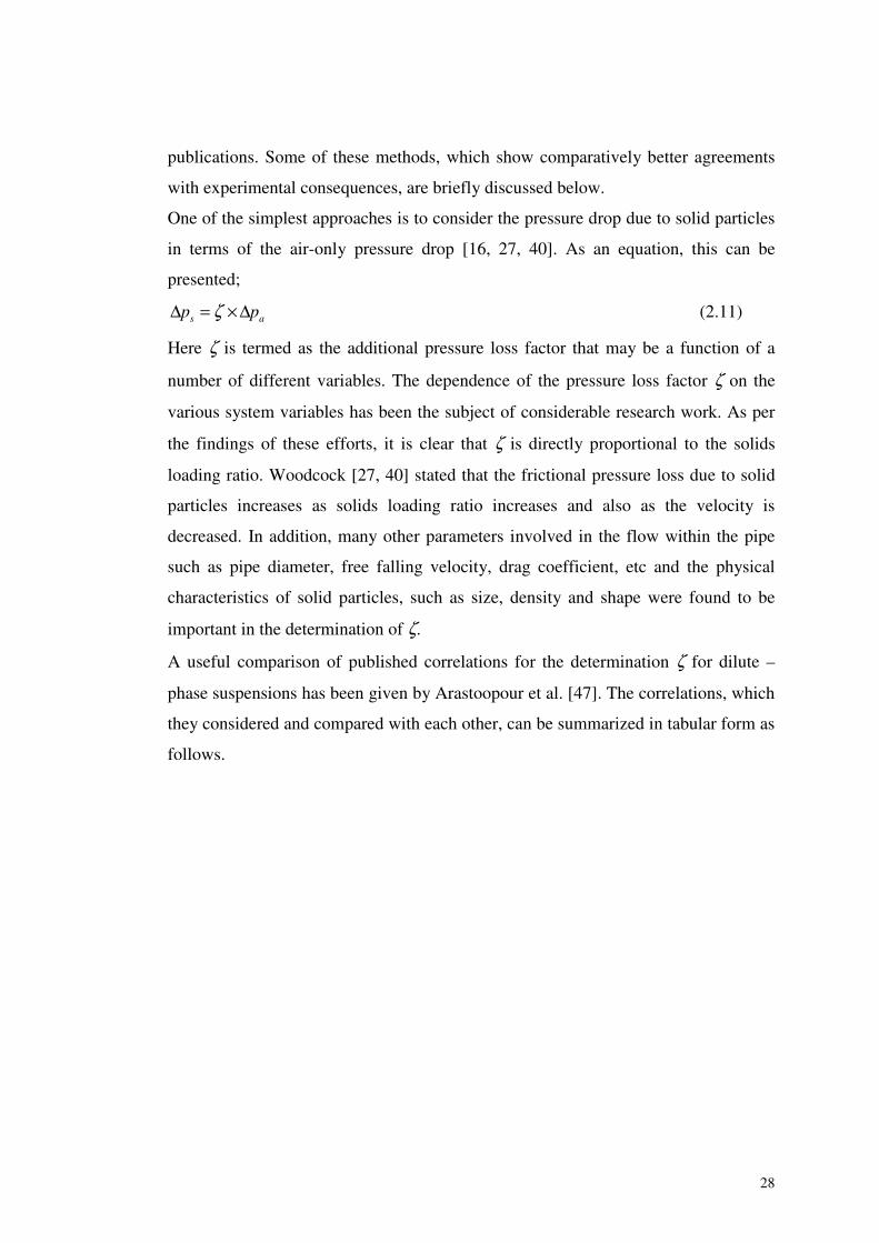
A useful comparison of published correlations for the determination ζ for dilute –
phase suspensions has been given by Arastoopour et al. [47]. The correlations, which
they considered and compared with each other, can be summarized in tabular form as
follows.
29
Table 2.1: Available correlations to determine the additional pressure loss factor (ζ).
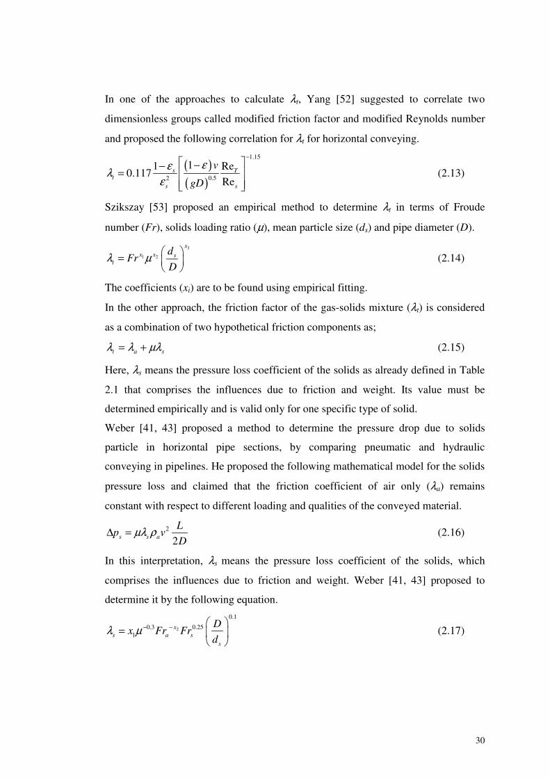
2.4.1.3 Solid Friction Factor
Another popular technique in the pressure drop determination of horizontal pipe
sections is ‘the solid friction factor method’, in which the pressure drop due to the
presence of solid particles, is analysed in a form analogous to single phase flow. In
this approach, the Darcy-Weisbach’s equation is modified such that λ is considered
either as the friction coefficient for the total flow or as a combination of friction
coefficients for the solid flow and the gas flow separately. When the friction factor of
gas-solid mixture is considered, the total pressure drop can be presented as below;
2
2t
t
Lvp
D
λ ρΔ = (2.12)
Equation Remarks
0.5
8s s
a a
λ ρπζ μλ ρ
= � ��
[48]
λs is called as solid friction factor
6.085.0 Re
0034.0
Re
026.0 +=sλ
s s
a a
v
v
λζ μλ
= [49] vs is solid velocity
12
s
s T
C m
v uζ = [50]
C1 is a factor depend on D and uT is
the free falling terminal velocity of
solids
2
2
1
Res
a
DC
d
ρζ μρ
= � ��
[51]Re is gas phase Reynolds number
and C2 is a constant
3 s
a s a T
C m g
Dv v uζ
ρ= [50]
A modification to the equation in 3rd
row
30
In one of the approaches to calculate λt, Yang [52] suggested to correlate two
dimensionless groups called modified friction factor and modified Reynolds number
and proposed the following correlation for λt for horizontal conveying.
( )( )
1.15
0.52
11 Re0.117
Res T
ts s
v
gD
εελε
−� �−−= � �� �� �
(2.13)
Szikszay [53] proposed an empirical method to determine λt in terms of Froude
number (Fr), solids loading ratio (μ), mean particle size (ds) and pipe diameter (D).
3
1 2
xx x s
t
dFr
Dλ μ = � �
� (2.14)
The coefficients (xi) are to be found using empirical fitting.
In the other approach, the friction factor of the gas-solids mixture (λt) is considered
as a combination of two hypothetical friction components as;
sat μλλλ += (2.15)
Here, λs means the pressure loss coefficient of the solids as already defined in Table
2.1 that comprises the influences due to friction and weight. Its value must be
determined empirically and is valid only for one specific type of solid.
Weber [41, 43] proposed a method to determine the pressure drop due to solids
particle in horizontal pipe sections, by comparing pneumatic and hydraulic
conveying in pipelines. He proposed the following mathematical model for the solids
pressure loss and claimed that the friction coefficient of air only (λa) remains
constant with respect to different loading and qualities of the conveyed material.
2
2s s a
Lp v
Dμλ ρΔ = (2.16)
In this interpretation, λs means the pressure loss coefficient of the solids, which
comprises the influences due to friction and weight. Weber [41, 43] proposed to
determine it by the following equation.
2
0.1
0.3 0.251
xs a s
s
Dx Fr Fr
dλ μ −− = � �
� (2.17)
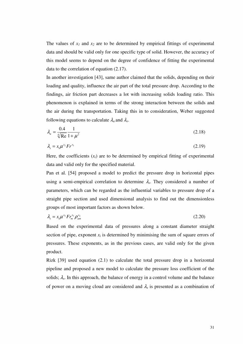
31
The values of x1 and x2 are to be determined by empirical fittings of experimental
data and should be valid only for one specific type of solid. However, the accuracy of
this model seems to depend on the degree of confidence of fitting the experimental
data to the correlation of equation (2.17).
In another investigation [43], same author claimed that the solids, depending on their
loading and quality, influence the air part of the total pressure drop. According to the
findings, air friction part decreases a lot with increasing solids loading ratio. This
phenomenon is explained in terms of the strong interaction between the solids and
the air during the transportation. Taking this in to consideration, Weber suggested
following equations to calculate λa and λs.
24 1
1
Re
4.0
μλ
+=a (2.18)
321
xxs x Frλ μ= (2.19)
Here, the coefficients (xi) are to be determined by empirical fitting of experimental
data and valid only for the specified material.
Pan et al. [54] proposed a model to predict the pressure drop in horizontal pipes
using a semi-empirical correlation to determine λs. They considered a number of
parameters, which can be regarded as the influential variables to pressure drop of a
straight pipe section and used dimensional analysis to find out the dimensionless
groups of most important factors as shown below.
32 41
xx xs m amx Frλ μ ρ= (2.20)
Based on the experimental data of pressures along a constant diameter straight
section of pipe, exponent xi is determined by minimising the sum of square errors of
pressures. These exponents, as in the previous cases, are valid only for the given
product.
Rizk [39] used equation (2.1) to calculate the total pressure drop in a horizontal
pipeline and proposed a new model to calculate the pressure loss coefficient of the
solids; λs. In this approach, the balance of energy in a control volume and the balance
of power on a moving cloud are considered and λs is presented as a combination of
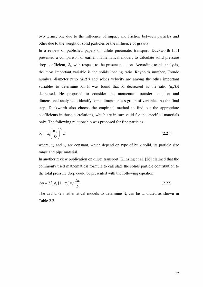
32
two terms; one due to the influence of impact and friction between particles and
other due to the weight of solid particles or the influence of gravity.
In a review of published papers on dilute pneumatic transport, Duckworth [55]
presented a comparison of earlier mathematical models to calculate solid pressure
drop coefficient, λs, with respect to the present notation. According to his analysis,
the most important variable is the solids loading ratio. Reynolds number, Froude
number, diameter ratio (dp/D) and solids velocity are among the other important
variables to determine λs. It was found that λs decreased as the ratio (dp/D)
decreased. He proposed to consider the momentum transfer equation and
dimensional analysis to identify some dimensionless group of variables. As the final
step, Duckworth also choose the empirical method to find out the appropriate
coefficients in those correlations, which are in turn valid for the specified materials
only. The following relationship was proposed for fine particles.
2
1
x
ps
dx
Dλ μ = � �
� (2.21)
where, x1 and x2 are constant, which depend on type of bulk solid, its particle size
range and pipe material.
In another review publication on dilute transport, Klinzing et al. [26] claimed that the
commonly used mathematical formula to calculate the solids particle contribution to
the total pressure drop could be presented with the following equation.
( ) 22 1s s s s
Lp v
Dλ ρ ε ΔΔ = − (2.22)
The available mathematical models to determine λs can be tabulated as shown in
Table 2.2.
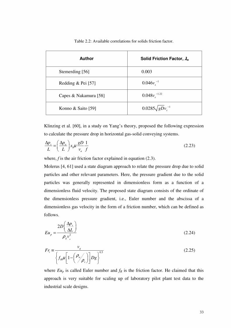
33
Table 2.2: Available correlations for solids friction factor.
Klinzing et al. [60], in a study on Yang’s theory, proposed the following expression
to calculate the pressure drop in horizontal gas-solid conveying systems.
1
1s a
a
p p gDx
L L v fμΔ Δ = � �
� (2.23)
where, f is the air friction factor explained in equation (2.3).
Molerus [4, 61] used a state diagram approach to relate the pressure drop due to solid
particles and other relevant parameters. Here, the pressure gradient due to the solid
particles was generally represented in dimensionless form as a function of a
dimensionless fluid velocity. The proposed state diagram consists of the ordinate of
the dimensionless pressure gradient, i.e., Euler number and the abscissa of a
dimensionless gas velocity in the form of a friction number, which can be defined as
follows.
2
2
a
s
pg
pD
LEu
vρ
Δ � �Δ� = (2.24)
0.5
1
gi
aR
s
vFr
f Dgρμ ρ
≡� �� � − � �� �� �� � �� �
(2.25)
where Eup is called Euler number and fR is the friction factor. He claimed that this
approach is very suitable for scaling up of laboratory pilot plant test data to the
industrial scale designs.
Author Solid Friction Factor, λλλλs
Stemerding [56] 0.003
Redding & Pei [57] 10.046 sv −
Capes & Nakamura [58] 1.220.048 sv −
Konno & Saito [59] 10.0285 sgDv −
34
In another extensive review, Arastoopour et al. [47] examined the published methods
of pressure drop calculations for dilute phase conveying. They classified all the
available correlations broadly in to two categorise. i.e.,
• Group 1, in which the ratio of total pressure drop to the pressure drop due to
gas alone,a
t
p
P
ΔΔ
is correlated (like in equation (2.11))
• Group 2, in which the total pressure drop is expressed as the summation of
pressure drops due to acceleration, wall friction, and gas-solids friction.
Arastoopour et al. [47] criticized the group 1 approach, because using a pipe of
different material and roughness, the total pressure drop will not change as much as
that for the gas alone and recommended the group 2, even though that group has the
similar problem with wall friction. They proposed the following model to determine
λs;
23
8a a s
s Ds p s
v vDC
d v
ρλρ
−= � ��
(2.26)
In group 2 approach, the total conveying line pressure drop is divided into several
components and focus on each of them separately, by considering their
distinguishable features. The pressure drop incurred in horizontal sections can be
determined by one of the analytical methods explain above. Another important
concept highlighted with this approach is the pressure drop relevant to the
acceleration region, which usually exists after some sudden change in flow direction
or flow restriction.
2.4.2 Acceleration Length and Pressure Drop
When the pressures drop determination of straight pipe is concerned, another
important aspect is the acceleration length and acceleration pressure drop. For any
pneumatic conveying system the particles must be feeded into the gas stream and
there exists a period over which the particles and gas are not at a steady state. During
the transport of gas-solid mixture, the particles undergo deceleration and
acceleration, whenever there is a direction change like bend or a flow restrictor like
35
valves. Researchers have found that this phenomenon contributes significantly to the
overall system pressure drop.
Mills et al. [62] published a research paper with a detailed review of models
available with regard to acceleration length. By monitoring the erosive wear of a
number of bends, they presented a technique to establish acceleration lengths that
showed a big influence of the conveying conditions and product characteristics, such
as particle size distribution, density and shape.
In a simple model, Woodcock et al. [27] suggested to treat the whole length of the
system as fully-accelerated flow and then to add on an appropriate extra pressure –
drop for each obstruction, which causes the acceleration/deceleration. This extra
pressure drop arises from the need to re-accelerate the solid particles after they have
been slowed down by the obstruction. This additional pressure component was
calculated by the following model.
s sA
m vp
AΔ = (2.27)
Duckworth [55] found the acceleration length/pressure drop an important parameter,
particularly in the case of short pipelines. He proposed the following two equations
to determine the acceleration length and pressure drop respectively, and claimed that
they are best for uniformly sized coarse particles of spherical shape having diameter
greater than about 600 μm.
3
1
2
12
1
2
5
2
16
���
�
�
���
�
�
��
���
��
���
���
���
�
=
ρρ
ρ
s
pa
sA
d
D
Dg
m
D
L(2.28)
2
2s a
A A Ba
m vp
m
ρ φ φΔ = (2.29)
where, φA and φB are dimensionless parameters relating2 2
2a
p s
v
gd
ρρ
� �� ��
and θ (angle of
pipeline inclination) respectively.
36
By dividing the total pressure drop into several components, Marcus [63] proposed
the following model to calculate the acceleration pressure drop.
20.5 sA a
a
vp v
vμ ρ
Δ = +� �
� (2.30)
2.4.3 Dense Phase Transport
As discussed early in Chapter 1, the use of the term ‘Dense Phase’ is far from being
precise. Some have used the word in pneumatic conveying to mean solid particles
flowing at a velocity less than their saltation velocity. Some researchers have used
the phase diagram to designate the region to the left of the minimum pressure drop
curves as the dense phase region of flow. In spite of these discrepancies in definitions
of the dense phase conveying, it has been the main subject of considerable number of
theoretical and experimental research works over a substantial period of time.
Because of the number of advantages over dilute phase transport, this has been
acquiring more industrial applications during the past period of time. In particular,
the low rates of pipe wear and particle attrition that are obtained with the low
velocities involved and less air requirement thus the low power consumption are
among the advantages of dense phase conveying. But, unfortunately, there are
number of uncertainties, design difficulties and unforeseen pipe blockages, most of
which arise from the fact that the precise mechanism by which the particles are
conveyed has never been well understood.
Among the vast number of literatures on dense phase conveying, few of them, which
show a comparatively good agreement with the experimental data and are well
documented, has been selected for this study. In this section, the models on
horizontal dense phase conveying are considered and the vertical sections and the
velocity concepts will be discussed in their respective sections.
The work done by Konrad et al. [64] could be seen as one of the earliest and
frequently cited publication by fellow reseachers. They developed a theoretical
model to predict the pipeline pressure drop in horizontal dense phase plug conveying.
They describe the flow mechanism with following phenomenal concepts.
37
• The material is conveyed only in the plugs and in the regions just in front and
behind them.
• There is a layer of stationary material between the plugs.
• The flow pattern is similar to that of a gas-liquid system.
The proposed model for the pressure drop in horizontal pipe section can be presented
in following equations;
5.0
168.22
��
�
+=Δ
gD
uKg
L
p smwww
ss
μμρ
(2.31)
Where,( )
( )
21
1
s
s ssm s
s
s s
m
Auu u
m
Au
ρ
ρ
� �−� �� �=� �−� �� �
; ⎯us is the mean particle velocity
Basically, this model predicts a linear pressure loss behaviour with the plug length.
Konrad [65] stated that the overall conveying pressure difference increases
exponentially with pipeline length and emphasized the significant contribution of the
compressibility of the carrier gas. He described the expansion of gas inside the
pipeline as an isothermal process. Konrad [65] proposed a modification to equation
(2.31) by replacing its constants (i.e., 2 and 2.168) with the correlation coefficients,
which have to be determined empirically. Similarly, he used an integration method to
calculate the overall pressure drop in the pipeline.
For the plug flow conveying, Klinzing et al. [6] have used another form of an
integration equation to calculate the pressure on the pipeline referring to a
publication by Weber (published in German).
( ) ( ) ( )21 1
2s
sp a ss p
dp x xv v
dL d
ρελε−= − (2.32)
where p(x) is the pressure and ρ(x) is the relevant density of carrier fluid at L=x and
λsp is given in graphical form as a function of Rep.
Legel et al. [66] investigated the plug conveying of cohesion less materials and
introduced the transmission ratio of radial stress to axial stress, which is also called
38
the force (stress) transmission coefficient kw. The following model has been proposed
to calculate the pressure drop across a single plug.
pswpp gLFrp ρφtan)6.21( 2.0+=Δ (2.33)
Here, the suffix ‘p’ means the specified parameter related to the plug.
Mi and Wypych [67] proposed some modifications to Konrad’s model, challenging
the applicability of Ergun’s equation in slug flow. It was observed that, although
there is a relative motion between the slug and the pipeline wall, there is no relative
motion between the particles within the slug. They emphasized that the slug flow
situation is closer to a fluidised bed than a packed bed. Also, they used a well known
theoretical approach called Mohr’s circle analysis to determine kw and developed a
semi-empirical model to calculate the pressure drop, which can be used to optimise a
pneumatic conveying system. They presented it to determine the pressure gradient in
a single horizontal slug, as shown below.
fww
wsm D
kgp σμμρδ 4
2 += (2.34)
where, σf is given by;
2f c s sA vσ ρ= (2.35)
where, Ac is the cross sectional area ratio of stationary bed to pipe and vs is the slug
velocity. To determine Ac, the procedure proposed by Konrad et al. [64] was used
and where as an empirical method was used to determine vs by correlating it with
superficial air velocity and minimum air velocity for horizontal flow.
From a theoretical analysis, Mi et al. [67] suggested the following relationship for kw.
)cos(sin1
)cos(sin1
ws
ws
x
rwwk
φωφφωφ
σσ
−+−−
== (2.36)
wheres
w
φφω
sin
sinsin = and φs is the static internal friction angle, which is defined by
31
3
4bws γφφ = ; γb is the bulk specific gravity of solid.
They assumed that the sum of the pressure drop caused by the all slugs was equal to
that caused by a single slug having a total length equal to all the small slugs, as long
39
as the mean condition (based on average air density) were used. With this basis, the
following was used to determine total length of slugs in the pipeline.
(1 )s
sc s s
m LL
A A vρ=
−(2.37)
Their final expression for the pressure drop of total pipeline length can be presented
as below.
( )0.5 0.5 21 1.084 0.542 w s
ws
g m Lp k Fr Fr
Av
μ−Δ = + + (2.38)
An iterative procedure, by assuming a preliminary pipeline pressure drop and
continuing until convergence is obtained was recommended for practical
applications. Elsewhere, Mi et al. [68] and Pan et al. [69] have presented the
applicability of this method for nine different materials.
Based on this investigation, Pan et al. [23] published another work on dense phase
conveying. They modified equation (2.35) as shown below.
ppssf UUU )( −= ρσ (2.39)
where Up is the average particle velocity in the slug.
The gas-liquid analogy was used to determine Up and the resultant equation for the
pressure drop in a single slug was presented as;
)175.12(168.2 wwsswwsm kgD
gUkp −+= μρμρδ (2.40)
With the help of specific vertical test chamber and the packed bed model which
relates the overall pressure drop to the slip between the gas and the particles, an
empirical method was used to determine Us. Then, the overall pressure drop is
proposed below;
sm Lpp δ=Δ (2.41)
Here Ls is determined by the equation (2.37).
Matsuda et al. [70] proposed a model which is similar to the dilute phase approach
i.e, by hypothetical splitting of total pressure drop into two components as air only
and solid pressure drop. They found a direct relationship between Froude number
and solids friction factor and suggested an empirical fitting method to determine it.
40
2
1xs
Fr
x=λ (2.42)
Here, the values of x1 and x2 are to be determined by empirical method and valid only
for the specified material.
Referring to the model proposed by Muschelknautz and Krambrock (published in
German) considering the expansion of gas inside the pipeline as an isothermal
process, Marcus [63] proposed a step wise trial and error method to calculate the
pressure drop in plug flow dense phase transport. Here, the overall conveying
pressure difference is assumed to be increased exponentially, thus the model can be
presented as;
��
���
=
mk
aw
e
i
RTC
MLg
P
P φμ tanexp (2.43)
where, smk
a
UC
U=
Finally, equation (2.44) can be used to determine the total pressure drop, provided
the exit pipeline air pressure.
��
���
−=Δ 1
e
ie P
PPp (2.44)
Although Marcus [63] considered Cmk as a constant, Konrad [65] described it as a
strong function of μ(ρ/ρs) and it increased with both increasing μ and with
decreasing particle size. Based on equation (2.43) and assuming the isothermal
expansion of carrier gas, Konrad [65] proposed an integration method to determine
pressure P at a distance l from the outlet of the pipe (where the pressure is
atmospheric, Pa) as follows.
�=
=−l
l
a dlPfPP0
)( (2.45)
By explaining the interaction mechanism between suspension and sliding bed, Hong
et al. [71] carried out an experimental work. They considered the dilute phase
suspension and sliding bed separately and presented a model to calculate total
pressure gradient in stratified flow situations. They have used very simple pipeline
41
configuration with an 8m long pipe with a diameter of 20mm to transport sand and
lime, under a wide range of solids loading from 30 to 200.
Woodcock and Mason [72] proposed a simple model for stratified flow conveying,
referring to Muschelknautz and Krambrock (published in German).
( ) dsc gfLAp ρ−=Δ 1 (2.46)
where, fd is a friction coefficient for the sliding and rolling product.
Werner [73] found a direct influence of the size distribution of conveyed material to
the pressure drop and suggested a different approach. He proposed the following
equation to calculate the pressure drop in the pipeline, in general valid for the dense-
phase, starting from a power balance for the complete air-solid flow.
1( sin )
1s
s mk
p g LC
ρ λ θρμρ
� �� �Δ = +� �+� ��
(2.47)
Detecting an influence of particle size distribution, he used the following formulae to
determine λ and Cmk, i.e., friction factor and velocity ratio;
21
( , )CC
m ms
s
d df Fr
D dλ μ
=� �� �� �
(2.48)
3 4
( , )C C
smk s
m m
dDC f Fr
d dμ
=� � � �
� � (2.49)
where, dm and ds are mean particle diameters when arithmetically weighted and as
reciprocal value of the surface respectively. He suggested an empirical fitting method
to determine Ci.
For his data, the models for λ and Cmk are shown below;
( )0.20.3
50.25 7.82 10 m ss
m
d dFr
D dλ μ
−− = + × � �� �
� � (2.50)
( )0.20.3
0.59921 m s
mk sm
d dC Fr
D dμ
−− = � �� �
� � (2.51)
42
From the above equations, it is clear that the particle size distribution has a
considerable effect on friction factor and velocity ratio of the phases.
Molerus [4, 61] proposed a state diagram aprroach for rather coarse-grained particles
in strand flow. He defined the strand flow as a flow with rope-like clusters or
aggregate of particles. Considering mass and momentum balances on a moving
strand and assuming that the quality of material conveyed in the suspended phase is
negligible in comparison with that conveyed in the strand, an equation for the
additional pressure drop required to convey the strand was developed. This analysis
leads to the realization that the volumetric loading and not the solids loading is the
important factor in determining the stability of a system. Here, the pressure gradient
due to the solid particle is generally represented in dimensionless form and is
represented as a function of the volumetric flow ratio, voidage and the friction
number which can be defined as flows;
( )( ) ( ); ;1 1
s
gs
R s a s s s
p
L f Frif g
ρ με
ρ ρ ε ρ ε
Δ� �Δ = � �− − −� �� �
(2.52)
Where;
[ ]0.5
1 1
g
sR s
a
UFri
f Dgρ ερ
≡� �� � − −� �� �� �� � �� �
(2.53)
The proposed state diagram consists of friction number as the abscissa and
dimensionless pressure gradient over the frictional resistance of the strand as the
ordinate. The diagram contains two other additional parameters, the volumetric flow
ratio, i.e., ( )1g
s s
Cρ μ
ρ ε=
−and the ratio of the strand velocity w to the gas velocity Ug
above the strand in the form of curved lines. In the state diagram, the regions of
stable strand type conveying and the transition to plug flow can be clearly identified.
Klinzing et al. [6] used the frictional approach as discussed in dilute phase conveying
and utilized the following equation to calculate the solid friction factor for dense
phase conveying.
43
0.10.250.30.52 ps
sa
dFr
Fr Dλ μ
−−
= � ��
(2.54)
2.5 Vertical Pipe Sections
Same as the horizontal sections, vertical sections are also very important in
pneumatic conveying systems. Particularly, when there is a height difference
between the sending source and the receiving station, at least one vertical section is
inevitable. A quite large number of researches relavant vertical pipes can be seen in
open literature. Recently, there has been a trend to use inclined pipe sections instead
of vertical section. In the first section this chapter, the available models and theories
related to the vertical section are discussed and in the second half the inclined
sections will be focused on.
In contrast to horizontal gas-solid flow, vertical flow is very unstable, especially in
the case of cohesionless particles. This is because the gravitational force essentially
tends to collapse the plug, which makes the flow pattern very complicated. In
addition, vertical gas-solid two-phase flow is heterogeneous in nature and always
also locally unsteady. Particularly, when the solids volume fraction increases,
particles no longer flow as individuals but form groups of particles. This behaviour
has been detected by many researchers [6, 72, 74-76] and those loose particle groups
are called, according to their shape, clusters, streamers or sheets. It differs from the
horizontal pipe in that the complexity of stratification under gravity is replaced by
the three-dimensional behaviour, including possible recirculation. In many cases, the
particle groups are not all moving upwards, rather considerable downflow may be
observed, especially near the wall.
In case of vertical sections, the different flow behaviours called lean or dilute- phase
and dense-phase can be seen as in horizontal sections. The term ‘choking’ has
generally been used to describe a particular change in the flow behaviours when a
pneumatic conveying flow collapses into a relatively dense condition. At low
pressure drops, the solid is conveyed in the form of strands and clusters whereas, at
high pressure drops, the solid is transported as migrating fluidised bed that is in the
44
regime of the so-called fluidised bed conveying. A sudden increase in pressure drop
produces an equally sudden change in flow pattern. The superficial gas velocity
corresponding to this transition is referred to as the choking or critical velocity.
Consequently, the velocity determination plays a very important role in vertical
section. In this section, mainly the available models for the pressure drop
determination of verticle sections are addressed.
In a simple approach, Woodcock [40, 72] proposed to modify equation (2.11) to
compensate a vertical section as follows;
as a g v
a T
up p g L
u uζ ρ μ
Δ = Δ + � �−�
(2.55)
In one of the earliest approach to calculate the pressure drop in vertical lines, λt,
Yang [77] recommended that the total pressure drop should be considered as a
combination of different contributions due to acceleration, gravity and wall friction.
To determine λs for a vertical flow, Yang [77] proposed the following models for
different air velocity values.
( )0.979
3
1 Re0.0126 1
Res T
s ss p
ελ εε
−� �−= −� �� �� �
for 1.5a
T
v
v� (2.56)
( )1.021
3
1 Re0.041 1
Res T
s ss p
ελ εε
−� �−= −� �� �� �
for 1.5a
T
v
v� (2.57)
Where1
ReT Tdv ρμ
= and1
Re ( )p a sd v v ρμ
= −
Based on the above approach, Rautiainen et al. [75] considered the frictional pressure
drop by subtracting the static head and gas only frictional pressure from the total
pressure drop. It was revealed that for a constant gas velocity, as the solids mass flow
rate increases, then the friction pressure loss increases respectively at high gas
velocities but at the low gas velocities the reverse applies. In some cases, the friction
pressure loss is less than the friction pressure loss for gas only. It means that the solid
friction factor becomes negative corresponding to the low values of gas and solid
velocities. This phenomenon was supported by the visual observation, which showed
45
that at high gas velocities all the particles moved upward, but at low gas velocities
some of the particles flowed down near the wall.
Weber [41], in a comparison study between hydraulic and pneumatic conveying,
suggested the following relationship for vertical λs.
1 2
1200a
ss
v
v Frλ � �= +� �� �
(2.58)
Tsuji et al. [76] carried out an experiment to investigate the frictional characteristics
of plug flow conveying in vertical pipe sections. They expressed their doubt about
the applicability of packed bed models (such as Konrad’s [64]) in vertical conveying,
because of its high instability. They considered the total pressure drop across a plug
as a summation of two components; Δp1, which is due to the flow contraction at the
end of the plug and Δp2, which is the ordinary packed bed pressure drop. The
following were proposed to determine these two components.
21 2
10.5 1 s
s
p vρε
Δ = −� ��
(2.59)
( )22 1 20.5 p s s sp d C v C vρΔ = + (2.60)
where constants C1 and C2 are given by;
( )2
1 2 3
1150 s
p s
Cd
ε με
−= and
( )2 3
11.75 s
p s
Cd
εε−
=
2.6 Inclined Pipe Sections
To replace a combination of a vertical pipe section and a horizontal section, inclined
pipe sections have often been used. This has been the topic of number of
experimental investigations [6, 78-81]. One of the main advantages of these
approaches is that these models have the potential to be used in both horizontal and
vertical pipes as generalised approaches. Aziz et al. [82] proposed the frictional
approach for the inclined sections as well and used the following equation to
determine the friction factor.
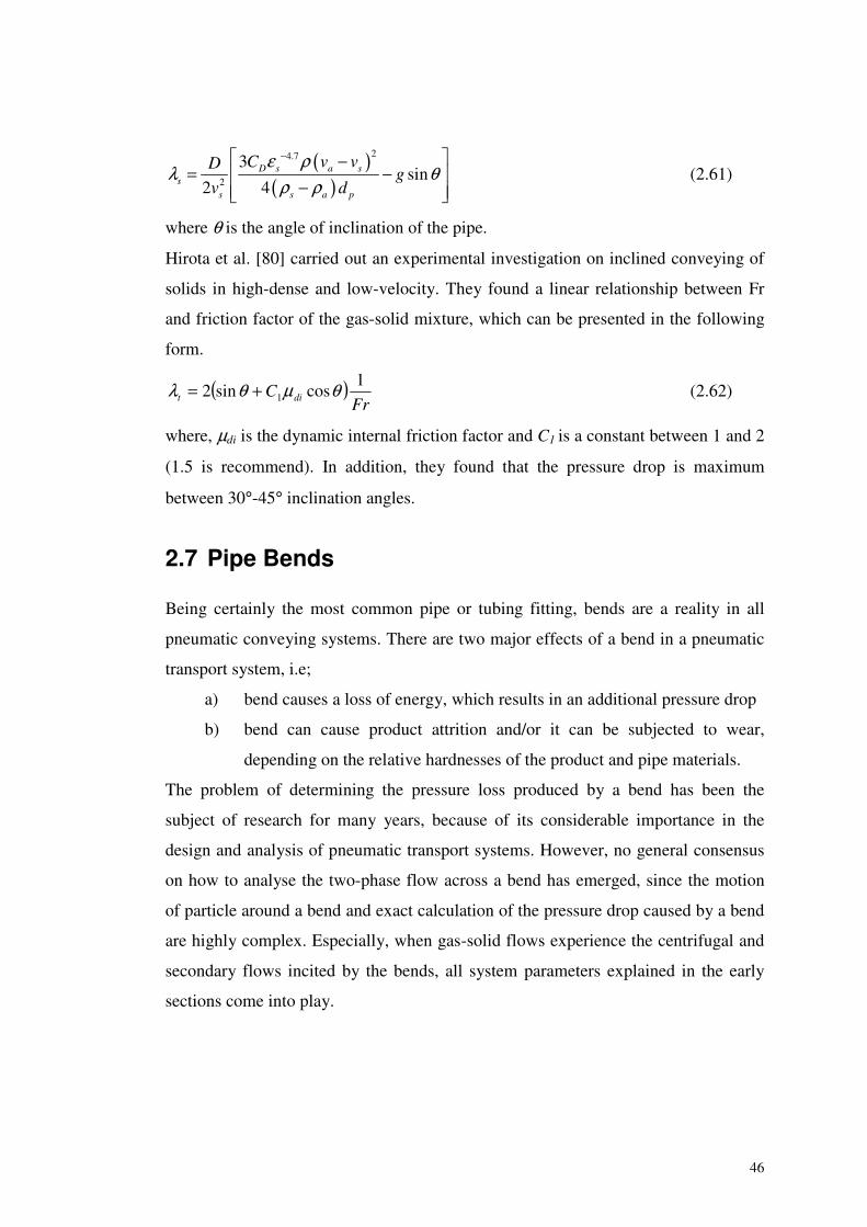
46
( )( )
24.7
2
3sin
2 4D s a s
ss s a p
C v vDg
v d
ε ρλ θ
ρ ρ
−� �−= −� �
−� �� �(2.61)
where θ is the angle of inclination of the pipe.
Hirota et al. [80] carried out an experimental investigation on inclined conveying of
solids in high-dense and low-velocity. They found a linear relationship between Fr
and friction factor of the gas-solid mixture, which can be presented in the following
form.
( )Fr
C dit
1cossin2 1 θμθλ += (2.62)
where, μdi is the dynamic internal friction factor and C1 is a constant between 1 and 2
(1.5 is recommend). In addition, they found that the pressure drop is maximum
between 30°-45° inclination angles.
2.7 Pipe Bends
Being certainly the most common pipe or tubing fitting, bends are a reality in all
pneumatic conveying systems. There are two major effects of a bend in a pneumatic
transport system, i.e;
a) bend causes a loss of energy, which results in an additional pressure drop
b) bend can cause product attrition and/or it can be subjected to wear,
depending on the relative hardnesses of the product and pipe materials.
The problem of determining the pressure loss produced by a bend has been the
subject of research for many years, because of its considerable importance in the
design and analysis of pneumatic transport systems. However, no general consensus
on how to analyse the two-phase flow across a bend has emerged, since the motion
of particle around a bend and exact calculation of the pressure drop caused by a bend
are highly complex. Especially, when gas-solid flows experience the centrifugal and
secondary flows incited by the bends, all system parameters explained in the early
sections come into play.
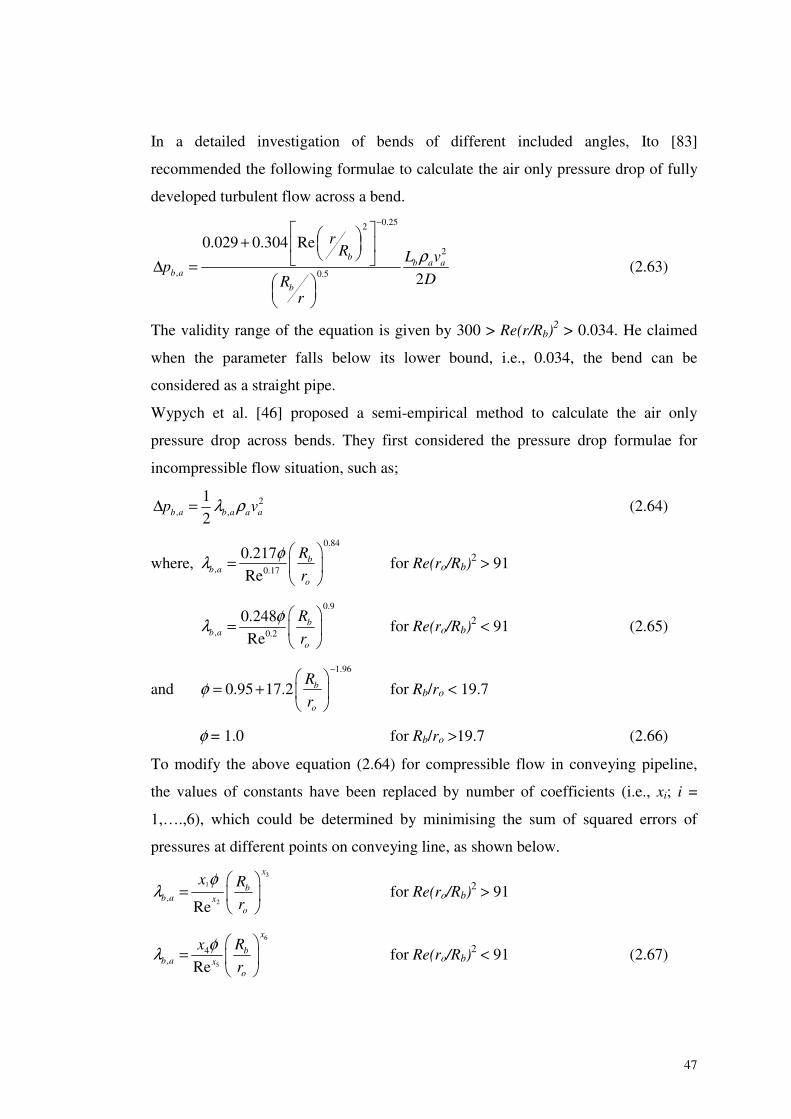
47
In a detailed investigation of bends of different included angles, Ito [83]
recommended the following formulae to calculate the air only pressure drop of fully
developed turbulent flow across a bend.
0.252
2
, 0.5
0.029 0.304 Re
2
bb a a
b a
b
rR L v
pDR
r
ρ
−� � + � �� �� � �Δ =
� ��
(2.63)
The validity range of the equation is given by 300 > Re(r/Rb)2 > 0.034. He claimed
when the parameter falls below its lower bound, i.e., 0.034, the bend can be
considered as a straight pipe.
Wypych et al. [46] proposed a semi-empirical method to calculate the air only
pressure drop across bends. They first considered the pressure drop formulae for
incompressible flow situation, such as;
2, ,
1
2b a b a a ap vλ ρΔ = (2.64)
where,0.84
, 0.17
0.217
Reb
b ao
R
r
φλ
= � ��
for Re(ro/Rb)2 > 91
0.9
, 0.2
0.248
Reb
b ao
R
r
φλ
= � ��
for Re(ro/Rb)2 < 91 (2.65)
and1.96
0.95 17.2 b
o
R
rφ
−
= + � ��
for Rb/ro < 19.7
φ = 1.0 for Rb/ro >19.7 (2.66)
To modify the above equation (2.64) for compressible flow in conveying pipeline,
the values of constants have been replaced by number of coefficients (i.e., xi; i =
1,….,6), which could be determined by minimising the sum of squared errors of
pressures at different points on conveying line, as shown below.
3
1
2,Re
x
bb a x
o
x R
r
φλ
= � �
� for Re(ro/Rb)
2 > 91
6
5
4, Re
x
bb a x
o
Rx
r
φλ
= � ��
for Re(ro/Rb)2 < 91 (2.67)
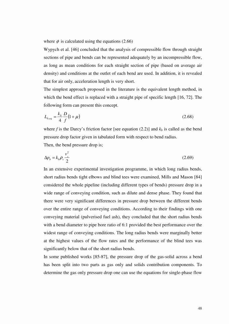
48
where φ is calculated using the equations (2.66)
Wypych et al. [46] concluded that the analysis of compressible flow through straight
sections of pipe and bends can be represented adequately by an incompressible flow,
as long as mean conditions for each straight section of pipe (based on average air
density) and conditions at the outlet of each bend are used. In addition, it is revealed
that for air only, acceleration length is very short.
The simplest approach proposed in the literature is the equivalent length method, in
which the bend effect is replaced with a straight pipe of specific length [16, 72]. The
following form can present this concept.
( )μ+= 14, f
DkL b
eqb (2.68)
where f is the Darcy’s friction factor [see equation (2.2)] and kb is called as the bend
pressure drop factor given in tabulated form with respect to bend radius.
Then, the bend pressure drop is;
2
2a
b b s
vp k ρΔ = (2.69)
In an extensive experimental investigation programme, in which long radius bends,
short radius bends tight elbows and blind tees were examined, Mills and Mason [84]
considered the whole pipeline (including different types of bends) pressure drop in a
wide range of conveying condition, such as dilute and dense phase. They found that
there were very significant differences in pressure drop between the different bends
over the entire range of conveying conditions. According to their findings with one
conveying material (pulverised fuel ash), they concluded that the short radius bends
with a bend diameter to pipe bore ratio of 6:1 provided the best performance over the
widest range of conveying conditions. The long radius bends were marginally better
at the highest values of the flow rates and the performance of the blind tees was
significantly below that of the short radius bends.
In some published works [85-87], the pressure drop of the gas-solid across a bend
has been split into two parts as gas only and solids contribution components. To
determine the gas only pressure drop one can use the equations for single-phase flow
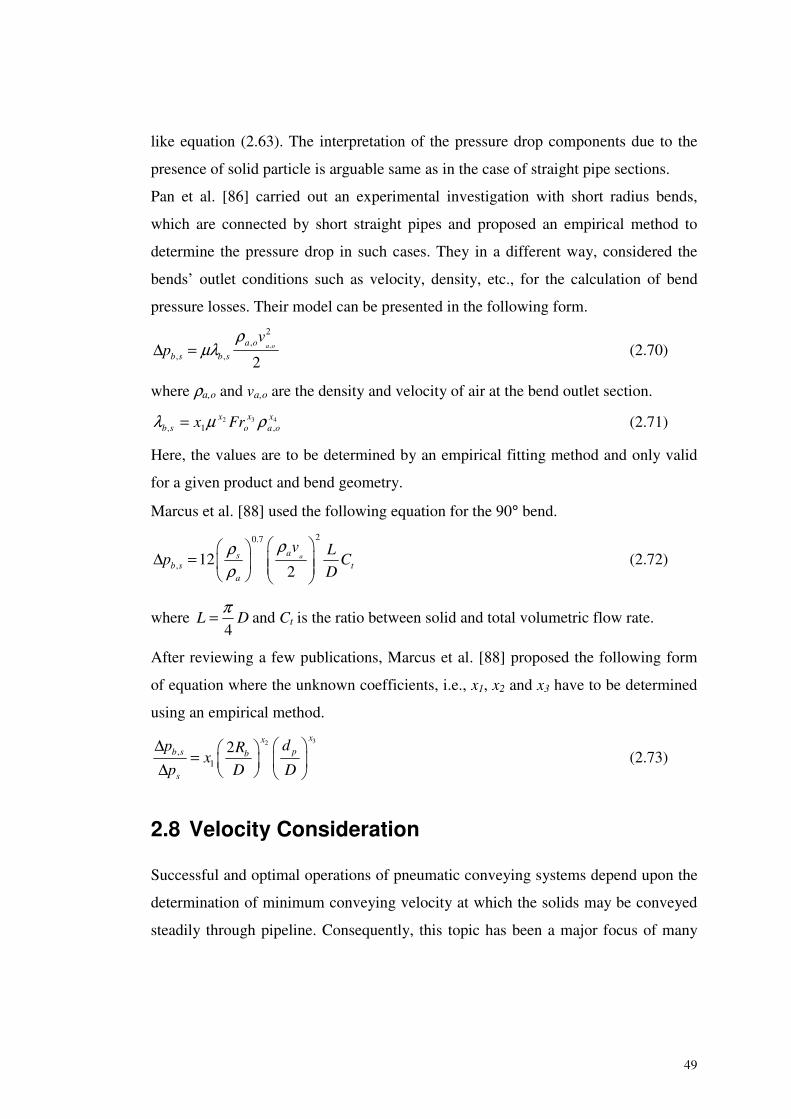
49
like equation (2.63). The interpretation of the pressure drop components due to the
presence of solid particle is arguable same as in the case of straight pipe sections.
Pan et al. [86] carried out an experimental investigation with short radius bends,
which are connected by short straight pipes and proposed an empirical method to
determine the pressure drop in such cases. They in a different way, considered the
bends’ outlet conditions such as velocity, density, etc., for the calculation of bend
pressure losses. Their model can be presented in the following form.
,
2,
, , 2a oa o
b s b s
vp
ρμλΔ = (2.70)
where ρa,o and va,o are the density and velocity of air at the bend outlet section.
432,1,
xoa
xo
xsb Frx ρμλ = (2.71)
Here, the values are to be determined by an empirical fitting method and only valid
for a given product and bend geometry.
Marcus et al. [88] used the following equation for the 90° bend.
20.7
, 122
aasb s t
a
v Lp C
D
ρρρ
Δ = � �� � � �� �
(2.72)
where4
L Dπ= and Ct is the ratio between solid and total volumetric flow rate.
After reviewing a few publications, Marcus et al. [88] proposed the following form
of equation where the unknown coefficients, i.e., x1, x2 and x3 have to be determined
using an empirical method.
32
,1
2xx
pb s b
s
dp Rx
p D D
Δ = � �� �Δ � � (2.73)
2.8 Velocity Consideration
Successful and optimal operations of pneumatic conveying systems depend upon the
determination of minimum conveying velocity at which the solids may be conveyed
steadily through pipeline. Consequently, this topic has been a major focus of many
50
research works, which have been produced a considerable number of publications in
open literature.
2.8.1 Determination of Minimum Conveying Velocity
In general, minimum-conveying velocity can be defined as the lowest safe gas
velocity for the horizontal transport of solids. If this gas velocity is set at the
beginning of the pneumatic conveying system (at the feed point), the gas velocity
will increase along the pipeline due to the compressibility effects, i.e. density
decrease, so the rest of the pipeline should be operating well above this lower
velocity bound. Keeping gas velocity above minimum conveying velocity in all
horizontal sections of a pipeline ensures no deposition of solids in the system and a
continuous and steady transport.
Over the years, many terms have been used to refer to minimum conveying velocity;
saltation velocity, pickup velocity, suspension velocity, deposition velocity, critical
velocity, velocity at the pressure minimum point of the general state diagram, etc.
Definitions of these terms are based on visual observations and pressure drop
measurements, and they are often applied to indicate some transition in the way in
which the particles are moving or begin to move. Unfortunately, a controversy exists
on how to define the minimum conveying velocity. The saltation velocity is usually
defined as the gas velocity in horizontal pipeline, at which the particles start to drop
out from suspension and settle on the bottom of the pipeline. The minimum gas
velocity in a system containing a horizontal pipeline that will prevent solids
deposition on the bottom of the pipeline is similar definition to the saltation velocity.
Pickup velocity has been defined as the gas velocity required for resuspending a
particle initially at rest on the bottom of a pipe or as the fluid velocity required to
initiate sliding, rolling and suspension of particles.
Although a considerable number of research works have been carried out in this
field, a general procedure to predict the minimum conveying velocity is not
available. Since a thorough understanding of the pickup and saltation mechanism has
not been possible yet, the theoretical predictions of pickup and saltation velocities
51
from the first principles have yet to be developed. However, some of the
experimental works, which give some theoretical correlations showing good
agreements with experimentally measured data, are discussed in subsequent chapters.
In one of the earliest addresses to the topic of saltation and minimum conveying
velocity, Zenz [14] defined the saltation velocity as the minimum fluid velocity
required to carry solids at a specified rate without allowing them to settle out in any
horizontal pipe section and thereby partially obstruct the flow area. He used the
dimensional analysis to correlate the saltation velocities of single particles in a
horizontal pipe to the free fall velocities. When both the saltation velocity and
terminal velocity are plotted, the difference is shown to be large at low Reynolds
numbers. To identify the influence of size distribution, he used the minimum and
maximum particle diameters of the size distribution and found an approximation to
the functional relationship between single particle saltation velocity and particle
diameter for the distribution. This is then incorporated into the correlation for
saltation velocity and solids feed rate in the following form.
( )1.50.21
gsogs gso
s
WUU U
Sρ Δ
= + (2.74)
where Ugs is the superficial air velocity at saltation, Ugso is the single-particle
saltation velocity, W is the solid flux (solid mass flow rate per unit pipe cross
section) and SΔ is the particle size and size distribution characteristic, which
represents the slope of a curve of single particle saltation velocity versus particle
diameter between the extremes of the largest and smallest particle in the mixture.
Cabrejos and Klinzing [34] carried out a detailed investigation to determine
minimum pickup velocity of different materials of different particle sizes (10 to 1000
μm) in a horizontal pipe, using visual observations. First they used a theoretical force
balance analysis and proposed the following equations to determine minimum pickup
velocity for large and small spherical single particles.
For a large single spherical particle;
0.51.54
13
p s s agpuo
D a
d f gdU
D C
ρ ρρ
� � � � −� �= − � �� �� �� � � �� � � �� �
(2.75)
52
For a small single spherical particle;
( )
2 0.51.5 7
4 33
121 8
3 6 3 35 3
1.54 10 1
1.302 10 6.35 106
gpuo
gpuo
pD a p
s s a p a p
UdC d
D D
Uf gd d d
D
ρυ
π ρ ρ ρυ
−
−
− −
� � � � � �× − � � � �� �� � � �
� � � �� �= − + × − ×� �� �� � �� �
(2.76)
Here, fs denote the coefficient of sliding friction. They proposed an iterative
procedure for equation (2.76). Combining the single-particle model with the
experimental results of a layer of particles, a general correlation was developed for
the minimum pickup velocity.
( )( )1 1 13 3 51.27 0.036 0.45 0.7 1gpu gpuoU Ar Ar Ar U
− −= + + + (2.77)
where 32
s ap
a
gAr d
ρ ρυ ρ
−= , which is called as Archimedes number, υ denotes the
carrier fluid kinematic viscosity.
The same authors elsewhere [35] proposed an empirically correlated equation to
determine the pickup velocity of coarse particles (above 100 μm). They used
dimensional analysis combined with their experimental findings, which show a
strong relationship to pickup velocity of horizontal pipe with the particle and pipe
diameters, and particle and carrier gas densities.
( )0.25 0.75
0.5 0.1750.0428 sgpu p s
p a
DU gd Re
d
ρρ
= � � � �� � � �
(2.78)
They claimed the validity ranges of this relationship as; 25<Res<5000,
8<(D/dp)<1340 and 700<(ρs/ρa)<4240.
In a seperate investigation, Cabrejos and Klinzing [89] studied pickup, saltation and
particle velocities in horizontal dilute-phase pneumatic transport. In the case of
pickup velocity, they emphasized the applicability of equation (2.78) published
elsewhere [35].
They proposed the following expression to predict the saltation velocity of coarse
particles with help of dimensional analysis.
53
1.25
0.50.00224 sgs gso p
a
U U gdρ μρ
− = � �
� (2.79)
where Ugs is the saltation velocity. In addition, they emphasized the influence of
particle diameter to saltation velocity highlighting that adhesive and cohesive forces
play a significant role in the case of fine particle, while friction and the particle
weight are more important for coarse particles.
In the same article, Cabrejos and Klinzing [89] highlighted that the particle velocity
increases as mean gas velocity increases, and particle velocity decreases as solids
flow rate increases, showing the importance of solids loading ratio on particle
velocity from the plots of particle velocity vs. velocity difference of saltation and
mean gas velocities. They proposed the following relationship to determine the
particle velocity.
( ) 2
1
x
s g gsU x U U= − (2.80)
The coefficients x1 and x2 best fitted the experimental results, were obtained using a
least squares technique.
Hayden et al. [90] followed a similar procedure as Cabrejos and Klinzing to
determine the pickup velocity for fine particles of size range 5-35 μm. According to
their findings;
• Pickup velocity remains relatively constant at very small particle diameters,
specially, less than 10 μm.
• Pickup velocities for non-spherical particles are higher due to particle
interlocking.
Molerus [4, 91] suggested to predict the minimum conveying velocity using the
following relationship;
( )4min0.018
1g
s s
Friρ
μρ ε
=−
(2.81)
where;
[ ],min
min 0.5
1 1
g
sR s
a
uFri
f Dgρ ερ
≡� �� � − −� �� �� �� � �� �
(2.82)
54
Here fR is the wall friction factor.
In a comparison study, Weber [92] tried to find out some hydraulic transport analogy
to the pneumatic conveying. He proposed the following relationships to determine
the minimum velocity for dilute suspension flow.
0.1
0.25min
87
3p
so
dFri u
Dμ
= + � �� �� �
for uso ≤ 3 m/s
0.1
0.25min 15 pd
FriD
μ
= � ��
for uso > 3 m/s (2.83)
where uso is the free settling velocity of a single particle.
However, the great complexity of the above equations, coupled with the fact that it
was developed from the data obtained in rather small-scale model tests, might well
discourage the use of this correlation for the design purpose.
2.8.2 Choking Velocity in Vertical Flows
The above discussion is mainly focussed on flow of horizontal pipe sections. When
the vertical sections are dealt with, the above mentioned models are no longer valid,
since the flow behaviour in vertical pipe is totally different from that in horizontal
sections, as discussed in section 2.5. In contrast to the term ‘saltation’ used in
horizontal pipes, most of the researchers, the term ‘choking’ has generally been used
to describe a particular change in the flow behaviour when a pneumatic conveying
flow collapses into a relatively dense condition in vertical sections. But
unfortunately, there is no clear-cut definition of choking available in the literature as
yet. However, three different mechanisms that trigger the choking were distinguished
in different investigations [93]. They can be detailed as follows;
a. Accumulative choking; which stresses the essence of solid accumulation at
the bottom of a vertical conveying tube
b. Classical choking; the sudden formation of slugs or plugs when a steady
operation ceases.
c. Pipe choking; due to the inappropriateness of the pipeline components.
55
Here, the types a and b are due to the inherent changes in gas-solid flow itself, while
the type c choking actually stems from facility inefficiency.
Yang [94] published a paper describing the choking phenomena, with the aim to
present a unique approach to calculating the choking velocity and choking voidage
by using readily available properties of the transported materials and system
characteristics. He expressed that the choking evolved as a result of range of
instabilities and defined it as the point where internal solid circulation, with solids
moving downward at the wall and moving upward in the core, began. Assuming that
the slip velocity is equal to the free-fall velocity at choking, he proposed the
following equation;
11
s
c t
t c
U
U u
u ε= +
−(2.84)
where Uc is the choking velocity.
Then, he assumed a constant value, i.e., 0.01 for solid friction factor at the choking
condition λs,c , and proposed the following equation;
( )[ ]
4.7
, 2
2 10.01
c
s c
c t
gD
U u
ελ
− −= =
−(2.85)
Since this assumption was arbitrary, later he proposed some modifications to
equation (2.85) as shown below;
( )[ ]
2.24.7
52
2 16.81 10
c a
sc T
gD
U u
ε ρρ
− − = × � �
− � (2.86)
2.8.3 Determination of Average Particle Velocity
When the particle velocity is considered, the other terms that come into the picture
are terminal velocity, slip velocity and voidage. Klinzing et al. [6] discussed these
parameters in detail and recommended the following relationships.
The actual carrier fluid velocity can be given in the following form when the voidage
is considered.
56
aa
s
Uu
ε= (2.87)
Slip velocity is the resultant velocity between the fluid and solid caused by the
particle-particle and particle-wall interactions and can be represented by the
following equation;
s a sw u u= − (2.88)
Another important velocity parameter of a two-phase flow is the particle terminal
velocity, which depends on the drag coefficient thus, on the Reynolds number as
well. There are number of different correlations available for different Re regions as
shown below.
( )2
18p s a
T
d gv
ρ ρη−
= for ReT <2.0
( )0.711.14 0.71
0.29
0.153 p s aT
a
d gv
ρ ρρ η
−= for 0.5< ReT <500
( ) 0.5
1.74 p s aT
a
d gv
ρ ρρ
� �−= � �
� �for 500 < ReT < 2×10⁵
( ) 0.5
3.65 p s aT
a
d gv
ρ ρρ
� �−= � �
� �for 2×10⁵ < ReT (2.89)
where vT is the terminal velocity and ReT is the Reynolds number related to vT.
To determine the solids velocity, Klinzing et al. [6] proposed the following
equations, referring some earlier work by Hinkle.
( )0.92 0.5 0.2 0..541 0.68s a p s av v d Dρ ρ− −= − (2.90)
They proposed another empirical correlations referring to Yang, as shown below.
0.524.71
2a s s
s fo ss
v vv w
gD
λ εε
= − +� �
� (2.91)
where, λs is the solid friction factor discussed in details in Section 2.4.1.3.
57
2.9 Scale Up Techniques
One method that is used for predicting pressure drop involves testing a sample of the
product to be conveyed in the final system in a pilot scale rig over a wide range of
operating conditions, and measuring the product and air flow rates and resulting
pressure drops. The obtained data are then scaled by experimentally determined
factors to predict the pressure drop in the full scale system. This method has the
advantage that real test data on the product to be conveyed in the projected system
are used for the design work. This is important because it provides useful
information about the conveyability of the product, as well as determining valuable
data on the minimum conveying velocity etc.
The scaling of test data is considered to be one of the most important stages of the
design process, in that it provides the link between laboratory-scale apparatus and
full-scale industrial installations. Hence, accuracy and reliability of scale-up are
essential.
Basically, there are two approaches in scaling up techniques available in literature;
the global testing approach and the piecewise approach. Both approaches have their
own advantages and undesirable characteristics as well.
2.9.1 Mills Scaling Technique
The basic condition of Mills’ [16] technique is that conveying conditions, in terms of
air velocities, should be identical for the pilot plant and full-scale plant. Since the air
velocity depends on the pressure and the air mass flow rate, the scaling has been
proposed to be carried out for the data points having the same conveying line
pressure drop and inlet air velocity. Here, the total pressure drop is considered as a
combination of pressure drop due to air alone and additional pressure drop caused by
the presence of the solid particles. Throughout, the whole scaling procedure, the
pressure drop due to solid particles is considered to be equal for the pilot plant and
full-scale plant.
The entire scaling procedure is to carry out in two stages; first stage involves scaling
to the required distance, with allowances for vertical sections and bends, while the
58
second stage scales the conveying characteristics in terms of the pipe diameter. The
concept of equivalent length of a bend has been introduced to compensate for the
different effects of bends in pilot plant and full-scaled plant.
2.9.1.1 Straight Horizontal Pipe Section
The horizontal pipe sections are considered to contribute directly to the equivalent
length of the whole conveying line, having the same magnitude as their physical
length.
For vertical sections, a scaling parameter is proposed in terms of length of straight
horizontal pipe sections. Since the pressure drop in vertical conveying is
approximately double of that in horizontal conveying, the equivalent length for the
vertical section is considered as,
vev LL 2= (2.92)
2.9.1.2 Effect of Bends
The same concept of a hypothetical equivalent length has been proposed for bends.
But, it is not an independent parameter as for the vertical sections. As a
simplification, the variation of equivalent length with velocity should be found for
the conveying material, using pilot plant.
,b eqL nb= (2.93)
2.9.1.3 Total Length
Considering the above relationships, the equivalent length of the whole conveying
line can be calculated. A model based on a reciprocal law has been proposed for
equivalent length of the pipeline as shown in equation (2.94).
1s
e
mL
∝ � ��
for a constant Δps and va.
That is,
59
��
���
=
2
112
e
ess L
Lmm (2.94)
Where, ebevhe LLLL ++= , for a constant Δps and va.
2.9.1.4 Pipe Diameter
A scaling model for pipe diameter is proposed, on the basis of pipe cross-sectional
area,
2DAms ∝∝ for a constant maD-2 and Δps.
Alternatively,
2
1
212 ��
���
=
D
Dmm ss (2.95)
and
2
1
212 ��
���
=
D
Dmm aa (2.96)
Mills suggested an iterative `trial and error´ procedure to determine the minimum
conveying limits, since conveying line inlet air velocity, pressure drop, airflow rate
and phase density (= ms/ma) are interrelated.
2.9.2 Wypych & Arnold Scaling Method
Wypych and Arnold [25] examined the validity of the scale-up procedure proposed
by Mills [16]. It has been revealed that the equations used in Mills scale-up technique
are inadequate, especially when data are scaled-up with respect to pipeline diameter.
They proposed following scale-up equation;
8.2
1
2
2
112 ��
���
′′
=D
D
L
Lmm ss (2.97)
Here, L�1 and L�2 represent the adjusted values of lengths to allow for any differences
between the number and type of bends used on the test rig and full-scale plant.
60
For the purposes of general design and feasibility studies, it is proposed to use
generalised pneumatic conveying characteristics. Using the data of pilot plant, the
co-ordinate system mfD-2 (abscissa) and Δps (ordinate) could be used to represent the
parameter msLD-2.8 for the purpose of generalising pipeline conveying characteristics.
In this investigation, the effects of pipeline bends are not considered and no
allowance has been made for the bends when pipeline lengths are calculated.
2.9.3 Keys and Chambers Scaling Technique
Keys and Chambers [95] proposed a scaling technique, based on empirical
correlations. It combines a number of non-dimensional flow parameters to predict the
pressure loss in the pipeline system.
2
2a
b
vp nB
ρΔ = (2.98)
To calculate the air alone friction factor, the following relationship was used.
( )2
2a
t ba
p pD
v Lλ
ρΔ −Δ
= (2.99)
An empirical correlation was obtained by plotting λa verses Re, in the form of the
following equation.
21 Rex
a xλ = (2.100)
To calculate solids friction factor;
( )2
2 t b as
g
p pD
v L
λλρ μ μΔ −Δ
= − (2.101)
Similar to the calculation of λa, the constants in the following equation should be
found by fitting empirical curves.
3 54.x x
s x Frλ μ = (2.102)
The pressure drop for the full-scale plant can be predicted with the following.
( )2
2g
predicted a s
v Lp
D
ρλ λ μΔ = + (2.103)
The authors emphasised that the effect of bends has to be considered when the solid
friction factor is calculated.
61
2.9.4 Molerus Scaling Technique
Molerus [91] proposed to consider a relationship between two non-dimensional
parameters given below;
2
2 s
pa a
p DL
vλ
μρ
Δ � �Δ� ≡ (2.104)
aa
vFr
Dg≡ (2.105)
where λp is called as the non-dimensional particle pressure drop and Δps is the
pressure drop due to the solid particle. Molerus [91] stated that the combination of
above two parameters defines fully suspended gas-solid pipe flow for given
combination of gas and particulate material. Based on this assumption, he proposed
to carry out pilot plant tests to get the data in terms of λp versus Fra and to use the
resulting curve for the prediction of the pressure drop of the plant to be designed.
2.9.5 Bradley et al. Scaling Technique
In a series of publications, Bradley et al. [96-101] formulated a piecewise scaling
technique for pneumatic conveying system designs. They use the concept of air only
and solid contribution to total pressure gradient of straight pipe sections. The concept
of suspension density also was used to categorise different flow conditions
experienced during conveying process.
Bradley [96, 97, 101] found a relationship for a pressure drop across bends, which
can be presented as shown below.
21
2b sus ap k vρΔ = (2.106)
Here ‘k’ is a dimensionless coefficient and ρsus is termed as suspension density which
is considered as the mean density of the gas-solid mixture in the pipeline. The value
of suspension density was simply calculated by dividing the solids flow rate by the
air flowing. It could be presented as shown in equation (2.107).
sus aρ μρ= (2.107)
62
He found that the variation of ‘k’ with superficial air velocity was similar in shape
for all of the radiused bends and could be represented by a single curve on a graph in
each case.
Hettiaratchi et al. [98] used the concept of suspension density to formulated a scaling
method for vertical pipe sections. They isolated the solid contribution to the total
pressure and then the solid pressure per unit suspension density was plotted versus
superficial air velocity. A constant trend was found between the above mentioned
quantities in the non-suspension transport region.
In similar line, Hyder et al. [100] investigated the effect of particle size on straight-
pipe pressure gradient in dilute-phase conveying. They used the relationship shown
in equation (2.108) to model the pressure gradient along straight pipe sections.
suss
dpk
dlρ =� �
� (2.108)
The value of ‘k’ was determined in terms of mean particle size.
2.10 Effects of Material Physical Characteristics
To describe a bulk material with the aim to understand its behaviour and
performances in pneumatic conveying systems, there are basically two major levels;
a. With the use of features of the material in its bulk form (cumulative/bulk
properties)
b. With the use of features of constituent particles (individual/singular
properties)
There are many descriptive terms and numerical parameters, which can be used in
the characterisation of conveying materials. The main properties that have been
identified as the most influential parameters on transport performances are briefly
listed below [72]:
• Particle size and size distribution – The natural force of attraction increases
with the decreasing particle size. Mean diameter, volume diameter, surface
diameter and Stokes diameter are few of the commonly used terms to define
the particle size.
63
• Particle shape – Usually, the shape of the constituent particles in a bulk solid
is an important characteristic as it has a significant influence on their packing
and flowing behaviour. Highly irregular shaped and fibrous particle can
interlock thereby increasing the resistance of a bulk solid to flow.
• Cohesiveness – This property gives a sort of an idea how strong the inter-
particle attraction forces, which can cause some problems in hopper
discharge, feeding and conveying as well.
• Hardness – The hardness is important when a pneumatic conveying
installation is being designed since it will give an indication of the need to
take steps to avoid undue erosive wear of the system components.
• Electrostatic charging – Due to some handling of bulk materials, constituent
solid particles acquire electrostatic charges. With electrostatic charges,
material may exhibit some cohesive properties.
As an early research on particle characterisation, Geldart [102] work, which has been
used as a base for many other experiments later, is worthwhile to take into account.
Based on experimental evidence, Getdart found that most products, when fluidised
by a gas, are likely to behave in a manner similar to one of four recognisable groups
and these groups of materials can be represented graphically as shown in Figure 2-1.
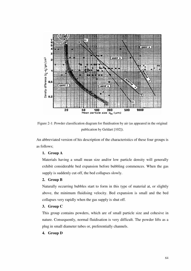
64
Figure 2-1: Powder classification diagram for fluidisation by air (as appeared in the original
publication by Geldart [102]).
An abbreviated version of his description of the characteristics of these four groups is
as follows;
1. Group A
Materials having a small mean size and/or low particle density will generally
exhibit considerable bed expansion before bubbling commences. When the gas
supply is suddenly cut off, the bed collapses slowly.
2. Group B
Naturally occurring bubbles start to form in this type of material at, or slightly
above, the minimum fluidising velocity. Bed expansion is small and the bed
collapses very rapidly when the gas supply is shut off.
3. Group C
This group contains powders, which are of small particle size and cohesive in
nature. Consequently, normal fluidisation is very difficult. The powder lifts as a
plug in small diameter tubes or, preferentially channels.
4. Group D
65
This group contains large and/or high-density particles. It is belived that the
bubble sizes may be similar to those in Group B and if gas is introduced only
through a centrally located hole, this group can be made to spout.
In later investigations, Dixon [103, 104] recognised that the fluidisation properties of
a product have significant implications with regard to its conveyability in dense
phase. His theoretical description enabled boundaries between expected flow
conditions to be drawn on the same axes as Geldart’s classification. It can be seen
that the boundaries between strong axisymmetric slugging, weak asymmetric
slugging and no slugging relate well to Geldart’s boundaries between groups D, B
and A. Dixon concludes that group A products are the best candidates for dense
phase conveying and, although not natural sluggers, can be made to slug using
commercially available equipment or systems. Group D products are also good
candidates because of their strong natural slugging behaviour. Group B products can
cause problems if high solids loading ratios are used and group C products are
possibly the least suitable materials for conveying in a dense phase mode.
Mainwaring and Reed [105, 106] found two parameters; permeability factor and de-
aeration factor can be measured with the help of small laboratory test rig to
understand the importance of the permeability and air retention characteristics of the
conveying material. They proposed a graphical method to determine the suitable
mode of conveying of particular material, by plotting the permeability factor, de-
aeration factor and pressure gradient together with minimum fluidising velocity. The
importance of above two factors were also empathised by Jones and Mills [107].
Goder et al. [108] examined the dependence of the transportability of a product in a
dense phase on the particle size, size distribution, moisture content and bulk density.
It was found that larger particles were less convenient for pneumatic conveying in
dense phase and addition of small fraction of smaller particles could increase the
transportability. Hyder et al. [100] reported the results of investigation whose aim
was compare the materials of similar particle densities, chemical composition and
shape. They found that as the particle size gets larger, the pressure losses along
straight sections of pipelines increase.
66
Pan [109] developed a flow mode diagram characterised by loose-poured bulk
density and mean particle diameter. The flow mode diagram classifies the bulk solid
materials into three groups; materials which can be transported smoothly and gently
from dilute to fluidised dense phase, materials that can be conveyed in dilute phase
or slug flow and bulk solids which can be conveyed only in dilute phase.
2.11 Computational Models
In the first part of this section, the computational model technique is described in
general and the multi-phase flow applications especially; pneumatic conveying
systems are then focused in connection with special methodologies adopted and
different applications.
The term CFD implies a computer-based simulation technology that enables one to
study the dynamics of things that flow, with the ultimate goal to understand the
physical events that occur in the flow of fluids around and within designated objects.
Using CFD, a computational model that represents a system or device to be studied
can be developed. Then, the fluid flow physics has to be applied to this virtual
prototype. Finally, the CFD software outputs a prediction of the fluid dynamics.
Being a sophisticated analysis technique, CFD not only predicts fluid flow
behaviour, but also some other phenomena such as transferring of heat and/or mass
(e.g.: dissolution, diffusion), changing phases (e.g.: freezing, boiling), chemical
reaction (e.g.: combustion), mechanical movement (e.g.: an impeller turning), and
stress or deformation of related solid structures (e.g.: wind loading). Hence, this
technique is very powerful and spans a wide range of industrial and non-industrial
application areas such as various engineering disciplines; mechanical, structural,
electrical, environmental, etc, and biomedical and meteorology fields as well [110].
There are number of unique advantages of CFD, which are compelling reasons to use
it against experiment-based approaches to fluid systems design. Those can be
described with the following features of CFD:
1. Insight - There are many devices and systems that are very difficult to
prototype, hence the controlled experiments are difficult or impossible to
67
perform. Often, CFD analysis shows parts of the system or phenomena
happening within the system that would not otherwise be visible through any
other means. CFD gives a means of visualizing and enhanced understanding
of designs.
2. Foresight - CFD is a tool for predicting what will happen under a given set of
circumstances, thus, it can answer many ‘what if?’ questions. With given
variables, it gives relevant outcomes quickly. In a short time, one can predict
how the design will perform, and test many variations until an optimal result
is arrived. Even that can be done before physical prototyping and testing and
gained practically unlimited level of detail results
3. Efficiency – There is a substantial reduction of lead times and costs of new
designs. CFD is a tool for compressing the design and development cycle.
To deal with the fluid flow systems, usually the CFD simulation codes are structured
around the numerical algorithms and comprise of basically three principal
components; pre-processor, solver and post-processor. A user-friendly interface,
which can be used to introduce the inputs of a flow problem to the solver algorithm
is employed in the pre-processing stage. The demarcation of computational domain,
grid generation, designation of fluid properties, boundary condition specifications
and problem specifications are usually performed in pre-processing level. Usually, a
solver uses one of the available streaming techniques: finite difference, finite element
and spectral method. Generally, three basic operations of a solver can be listed as
below:
a) Assume/approximate the unknown flow variable
b) Substitute the assumed variables in the governing flow equations and
discretisation [111]
c) Solve the differential equations
Post-processor stage comprises of the various means of data visualization tools, like
vector plots, contour plots, surface plots, particle tracking, animations, etc., to
visualize the output results of the problem.

68
2.11.1 Applications of CFD in Gas-Solid Flows
As explained in the early section, CFD is increasingly used in all branches of
engineering, including multi-phase flow applications like pneumatic conveying
systems. In this section, the general use of CFD in gas-solid flow systems, especially
in pneumatic transport, is described briefly.
CFD has proven to be extremely useful and accurate for a host of single-phase flows.
Indeed, it is now possible to make numerical predictions for many single-phase flows
that are more precise than the most accurate experimental local measurements that
can be obtained in a physical apparatus of the same geometry. CFD originally
applied to single phase flow problems, with advances in computer processing power
and more powerful numerical methods it can now be applied to more complex
situations. Multiphase flows involving a solids phase (or granular phases) have been
studied using this technique. Although the behaviour of solids has not been always
fully understood, attempts have been made to include granular phases into CFD
packages, by using approximations to describe the particle phase [112].
The CFD models of multi-phase flow problems are basically built on the principles
of the traditional way for modelling them, i.e., to use one-dimensional continuity and
momentum equations for each of the phases. Firstly by adding gas phase and solids
phase momentum equations together to obtain a mixture momentum equation, and
then by integrating the mixture momentum equation over the computational domain,
the differential equations reduce to a simple equation where the total pressure drop is
the sum of the pressure drops due to acceleration, gravity, and friction. Usually to
solve the equations, an iterative procedure is followed until a predefined residual of
convergence is achieved.
There are two fundamentally different approaches in numerical modelling of gas-
solid two phase flows according to the manner in which the particulate phase is
treated; Euler-Lagrangian and Euler-Euler granular approaches. The Lagrangian
model calculates the trajectories of individual or representative particles in the solids
phase, considering the velocity, mass and temperature history of them. In this
approach, for any interactions between the particles or with the boundaries of the
69
system, momentum is conserved and dissipation of energy is also possible. The
Eulerian approach simulates the granular phase as a continuous second fluid, and
solves a similar set of equations for the solids phase as for the fluid phase.
While CFD also holds great promise for gas-solid flows, obtaining accurate solutions
is much more challenging especially in dense phase situations, not just because each
of the phases must be treated separately, but, in addition, a number of new and
difficult factors come into play. For any gas-solid flow problem where the
concentration of dispersed phase is at least a few percent, the factors, such as; drag
and lift forces, slip or relative motion between the phases, inter-particle forces, etc,
have to be considered.
As a result, many different approaches, like; Eulerian, Lagrangian or combinations of
the two; interpenetrating two-fluid approach or discrete particles, etc, have been used
to model the multi-phase flow situations.. In addition, since the solids pressure
generated in Eulerian approach is not as easy to calculate as the equivalent fluid
pressure and a separate equation has to be used for closure in solution procedure.
Turbulence too is a problem, which is only partially solved by the introduction of the
concept of ‘Granular Temperature’. The granular temperature is a function of the
average difference between the individual particles velocity and the mean particle
velocity and defined according to the kinetic theory approach for granular flow
systems. The kinetic theory approach based on the oscillation of the particles uses a
granular temperature equation to determine the turbulent kinetic energy of the
particles, assumes either a Maxwellian or non-Maxwellian distribution for
instantaneous particle velocity, and defines a constitutive equation based on particle
collision and fluctuation. In fact, this approach allows the determination of solid
pressure and viscosity in place of the empirical equations.
Methods based on both Eulerian and Lagrangian approaches have difficulties in
accurately representing particle size distributions. To represent a full particle size
distribution, it is necessary to have a number of different particle phases, with
varying diameters and in similar proportions to the different sizes in the original
distribution [113]. This is a particular problem for the Eulerian methods, as each
extra phase requires that a new set of equations be solved.
70
2.11.2 CFD Applications in Pneumatic Conveying
A considerable number of publications on CFD applications on gas-solid systems can
be seen in open literature [81, 113-130]. The simulation works that are directly
related to pneumatic conveying systems are briefly described in this section.
One approach to simulate pneumatic transport system is the discrete element method
(DEM) based on an equation of motion for each individual particle. Pioneering
research in the development of the Lagrangian approach for the calculation of
pneumatic conveying has been performed by the group of Tsuji et al., [131-134]
especially with regard to modelling particle-wall collisions with wall roughness or
for non-spherical particles. Thus, in principle, individual particle size, shape and
density can be introduced directly into the equation. However this approach requires
huge computational time when many particles exist in the considered system. Later,
Tsuji [122] reported the developments of the discrete element method and suggested
a method to deal with large number of particles efficiently. Levy et al. [81] uses a
similar method to analyse the flow behaviours in vertical and inclined pipe sections,
with the help of a commercial software. A two-dimensional DEM was used by
Watano et al. [116] to analyse the particle movements, collision velocity, number of
collision, etc, in a pneumatic conveying process in order to compute the
electrification of particles during the transportation. A detailed summary of research
related to pneumatic conveying of particles in pipes or channels was recently
provided by Sommerfeld [135].
In another attempt to use a commercial software package for the prediction of
pneumatic conveying flow phenomena, Bilirgen et al. [127] compared the simulation
results with available experimental data from other sources. Levy [125] developed a
two-layer model to simulate plug flow in horizontal pneumatic conveying pipeline
and claimed that the model could be effectively used to predict the dense phase
behaviour. Later, Mason and Levy [126] used the same model to simulate dense
phase pneumatic transport of fine powders and claimed a good quantitative
agreement with experimentally determined pressure profiles for fully developed
flows in straight horizontal pipes. Pelegrina [124] used a one-dimensional steady-
71
state model for the simulation of pneumatic conveying of solid particles under
different conditions and determine the effects of the pipe diameter, air temperature
and inlet velocity on the pressure drop. A computational study of fully developed gas
–solid flow in a vertical riser is carried out by Yasuna et al. [119] in order to assess
qualitatively the predictive capacities of a computational model. Arastoopour et al.
[136, 137] considered particles of each size as a separate phase, developed an
experimentally verified particle-particle collision theory, introduced it in the one-
dimensional equations, and compared the calculated flow parameters with
experimental data for flow in dilute gas-solid systems. Mathiesen et al. [118]
developed a multi-fluid Eulerian model to describe the turbulence in solid phase
using the kinetic theory of granular flow. He proposed a model to enable a realistic
description of the particle size distributions in gas-solid flow systems. The model is
generalised for one gas phase and number of solid phases, characterising each solid
phase by a diameter, density and restitution coefficient. Li and Tomita [117] carried
out a numerical simulation for swirling and axial flow pneumatic conveying in a
horizontal pipe with an Eulerian approach for the gas phase and a stochastic
Lagrangian approach for particle phase, where particle-particle and particle-wall
collisions were taken into consideration.
72
3 EXPERIMENTAL SETUP ANDINSTRUMENTATIONS
For the experimental investigation, the pneumatic conveying test facilities available
in powder research laboratory (‘Powder Hall’) of the department of Powder Science
and Technology (‘POSTEC’) of Telemark Technological Research and
Development Centre (‘Tel-Tek’) has been used with some additional components to
accomplish the objectives of the work, since Telemark University College (‘HiT’)
has a close collaboration with Tel-Tek. Tel-Tek is a research foundation, which has
been functioning as a national organisation for industrial research, development
projects, technology transfer, academic research, etc.
This chapter gives a detailed description of the experimental setup used for the
investigation. As described in early chapters, the whole investigation was carried out
using different conveying pipeline configurations and instrumentations. The special
features added and modifications done to cater to the particular requirements of
individual sections of the investigation are described in relevant individual sections.
3.1 Available Pneumatic Transport Test Facilities at
POSTEC Powder Hall
The test rig has been designed with the objective of handling the research activities
of both the main transport modes, i.e., dilute and dense phase conveying. It mainly
consists of a top/bottom discharge blow tank of 3.5 m3, which can withstand a
maximum pressure of 10 bar g, a receiving tank of 2.6 m3 mounted on a special
arrangement of load cells to monitor the weight accumulation during the
experimentations, number of conveying pipes of different bore sizes and lengths,
various type of bends of different radii and configurations and a combination of a
screw type air compressor and a drier cum air cooler. The pipelines are laid out in
such a way that it is possible to have any combination of horizontal, inclined and
vertical sections depending upon requirements. The conveying line usually forms a
73
closed loop pneumatic transport circuit by placing the receiving tank on top of the
blow tank so that the particulate material under testing can be repeatedly tested
without taking it out of the test rig. In addition to these main items, number of
different measuring instruments like pressure transducers, flow transducers,
thermometers, humidity meters and an online sampler are also mounted on the
transport line in order to achieve the desired measurements. The transport rig is
equipped with facilities for continuous online data logging and visualising of data
like air pressure at various locations, air temperature, humidity, material transport
rate etc, on a real time basis. The data acquisition and analysis are undertaken with
the help of a user friendly software program of the LabVIEW® package. The test rig
facilitates with a control room where the operations of most of the valves, sampler
and data acquisition can be controlled by one operator.
3.2 Air Compressor
A screw type air compressor is used to supply the air requirement of the transport rig.
In this type of compressor, two helicoidal rotors, one with lobes and the other with
flutes, turn into each other and the first one turns 50 % quicker than the latter. The
inlet ends of the rotors are uncovered and the rotational motion of the rotor elements
sucks air to the compartment formed by the male lobe and a female flute. As the
rotors turn, the compartment becomes progressively smaller, thereby compressing
the entrapped air between the rotors and their housing. After successive compression
stages, air leaves at high pressure from the outlet port of the compressor [138] .
The technical data and specifications of the air compressor are given below.
• Production Company : Atlas Copco™
• Model : GA 1108
• Maximum working pressure : 8 bar
• Maximum air flow rate : 1000 Nm3/h
• Voltage/frequency : 380 V/50 Hz
• Maximum rotational speed : 1470 rpm
• Approximate thermal power : 106 kW
74
• Noise level : 66 dB
3.3 Dryer cum Cooler
The compressed air that goes into the dryer is pre-cooled in an air heat exchanger
using its own outgoing air to recover some energy loss. Then, the pre-cooled air is
directed to the evaporator where, by direct expansion of the refrigerant fluid, it is
cooled down to the dew point. At the dew point temperature, the compressed air has
the water condensates and oil, which exceed the corresponding saturation humidity.
Therefore, it goes then through a high efficiency condensate separator, which
eliminates them through an automatic drain system. The air cooled to its dew point,
finally circulates through the air to air heat exchanger in order to pre-cool the
compressed air coming in and at the same time acquire the final heating, which
makes the compressed air usable for the conveying process [33].
The outlet air from the refrigerant dryer approximately has the following qualities;
• the dew point : +3°C
• relative humidity : 25%
3.4 Control Valves
After the treatment of air in the refrigerant dryer, compressed air is supplied to the
main test rig through an array of valves, which controls and distributes the air supply
according to the requirements of the experimentations. Figure 3-1 shows a schematic
diagram of the air supply routes from the dryer to the main conveying line including
blow tank and for the operation of other accessories like mechanical filter at the
receiving tank and pneumatically driven valves.
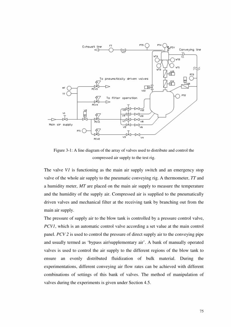
75
Figure 3-1: A line diagram of the array of valves used to distribute and control the
compressed air supply to the test rig.
The valve V1 is functioning as the main air supply switch and an emergency stop
valve of the whole air supply to the pneumatic conveying rig. A thermometer, TT and
a humidity meter, MT are placed on the main air supply to measure the temperature
and the humidity of the supply air. Compressed air is supplied to the pneumatically
driven valves and mechanical filter at the receiving tank by branching out from the
main air supply.
The pressure of supply air to the blow tank is controlled by a pressure control valve,
PCV1, which is an automatic control valve according a set value at the main control
panel. PCV 2 is used to control the pressure of direct supply air to the conveying pipe
and usually termed as ‘bypass air/supplementary air’. A bank of manually operated
valves is used to control the air supply to the different regions of the blow tank to
ensure an evenly distributed fluidization of bulk material. During the
experimentations, different conveying air flow rates can be achieved with different
combinations of settings of this bank of valves. The method of manipulation of
valves during the experiments is given under Section 4.5.
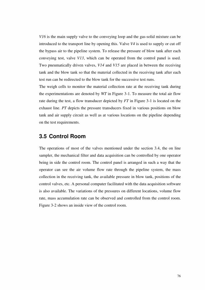
76
V16 is the main supply valve to the conveying loop and the gas-solid mixture can be
introduced to the transport line by opening this. Valve V4 is used to supply or cut off
the bypass air to the pipeline system. To release the pressure of blow tank after each
conveying test, valve V13, which can be operated from the control panel is used.
Two pneumatically driven valves, V14 and V15 are placed in between the receiving
tank and the blow tank so that the material collected in the receiving tank after each
test run can be redirected to the blow tank for the successive test runs.
The weigh cells to monitor the material collection rate at the receiving tank during
the experimentations are denoted by WT in Figure 3-1. To measure the total air flow
rate during the test, a flow transducer depicted by FT in Figure 3-1 is located on the
exhaust line. PT depicts the pressure transducers fixed in various positions on blow
tank and air supply circuit as well as at various locations on the pipeline depending
on the test requirements.
3.5 Control Room
The operations of most of the valves mentioned under the section 3.4, the on line
sampler, the mechanical filter and data acquisition can be controlled by one operator
being in side the control room. The control panel is arranged in such a way that the
operator can see the air volume flow rate through the pipeline system, the mass
collection in the receiving tank, the available pressure in blow tank, positions of the
control valves, etc. A personal computer facilitated with the data acquisition software
is also available. The variations of the pressures on different locations, volume flow
rate, mass accumulation rate can be observed and controlled from the control room.
Figure 3-2 shows an inside view of the control room.
77
Figure 3-2: The arrangement of control panel and PC inside the control room.
3.6 Pressure Transducers
A comparatively large number of pressure transducers have been used in the
experimentations to measure the pressure values at different points on the conveying
line. The type of pressure transmitter used in this investigation is called Cerabar S
and model PMC 731 manufactured by Endress+Hauser™. This type uses a rugged
ceramic diaphragm as the sensor and the deflection of the ceramic sensor caused by
the process pressure is transmitted to an electrode where the pressure-proportional
change in the capacitance is measured. The measuring range is determined by the
thickness of the ceramic diaphragm. The change in capacitance is then converted to
an analogue current signal by a built-in universal communication protocol and power
supply system called HART®. The technical details of the pressure transducers are
given below [139];
• Manufacturing Company : Endress+Hauser ™
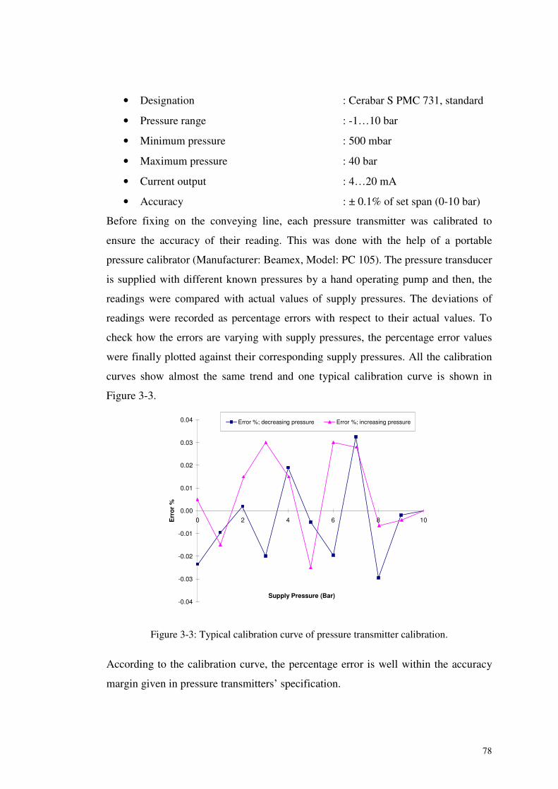
78
• Designation : Cerabar S PMC 731, standard
• Pressure range : -1…10 bar
• Minimum pressure : 500 mbar
• Maximum pressure : 40 bar
• Current output : 4…20 mA
• Accuracy : ± 0.1% of set span (0-10 bar)
Before fixing on the conveying line, each pressure transmitter was calibrated to
ensure the accuracy of their reading. This was done with the help of a portable
pressure calibrator (Manufacturer: Beamex, Model: PC 105). The pressure transducer
is supplied with different known pressures by a hand operating pump and then, the
readings were compared with actual values of supply pressures. The deviations of
readings were recorded as percentage errors with respect to their actual values. To
check how the errors are varying with supply pressures, the percentage error values
were finally plotted against their corresponding supply pressures. All the calibration
curves show almost the same trend and one typical calibration curve is shown in
Figure 3-3.
-0.04
-0.03
-0.02
-0.01
0.00
0.01
0.02
0.03
0.04
0 2 4 6 8 10
Supply Pressure (Bar)
Err
or
%
Error %; decreasing pressure Error %; increasing pressure
Figure 3-3: Typical calibration curve of pressure transmitter calibration.
According to the calibration curve, the percentage error is well within the accuracy
margin given in pressure transmitters’ specification.
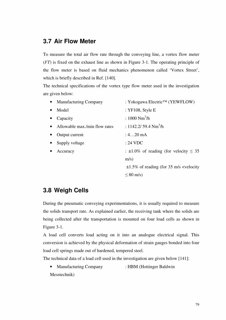
79
3.7 Air Flow Meter
To measure the total air flow rate through the conveying line, a vortex flow meter
(FT) is fixed on the exhaust line as shown in Figure 3-1. The operating principle of
the flow meter is based on fluid mechanics phenomenon called ‘Vortex Street’,
which is briefly described in Ref. [140].
The technical specifications of the vortex type flow meter used in the investigation
are given below:
• Manufacturing Company : Yokogawa Electric™ (YEWFLOW)
• Model : YF108, Style E
• Capacity : 1000 Nm3/h
• Allowable max./min flow rates : 1142.2/ 59.4 Nm3/h
• Output current : 4…20 mA
• Supply voltage : 24 VDC
• Accuracy : ±1.0% of reading (for velocity � 35
m/s)
±1.5% of reading (for 35 m/s <velocity
� 80 m/s)
3.8 Weigh Cells
During the pneumatic conveying experimentations, it is usually required to measure
the solids transport rate. As explained earlier, the receiving tank where the solids are
being collected after the transportation is mounted on four load cells as shown in
Figure 3-1.
A load cell converts load acting on it into an analogue electrical signal. This
conversion is achieved by the physical deformation of strain gauges bonded into four
load cell springs made out of hardened, tempered steel.
The technical data of a load cell used in the investigation are given below [141]:
• Manufacturing Company : HBM (Hottinger Baldwin
Messtechnik)
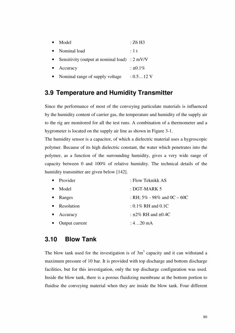
80
• Model : Z6 H3
• Nominal load : 1 t
• Sensitivity (output at nominal load) : 2 mV/V
• Accuracy : ±0.1%
• Nominal range of supply voltage : 0.5…12 V
3.9 Temperature and Humidity Transmitter
Since the performance of most of the conveying particulate materials is influenced
by the humidity content of carrier gas, the temperature and humidity of the supply air
to the rig are monitored for all the test runs. A combination of a thermometer and a
hygrometer is located on the supply air line as shown in Figure 3-1.
The humidity sensor is a capacitor, of which a dielectric material uses a hygroscopic
polymer. Because of its high dielectric constant, the water which penetrates into the
polymer, as a function of the surrounding humidity, gives a very wide range of
capacity between 0 and 100% of relative humidity. The technical details of the
humidity transmitter are given below [142].
• Provider : Flow Teknikk AS
• Model : DGT-MARK 5
• Ranges : RH; 5% - 98% and 0C – 60C
• Resolution : 0.1% RH and 0.1C
• Accuracy : ±2% RH and ±0.4C
• Output current : 4…20 mA
3.10 Blow Tank
The blow tank used for the investigation is of 3m3 capacity and it can withstand a
maximum pressure of 10 bar. It is provided with top discharge and bottom discharge
facilities, but for this investigation, only the top discharge configuration was used.
Inside the blow tank, there is a porous fluidizing membrane at the bottom portion to
fluidise the conveying material when they are inside the blow tank. Four different
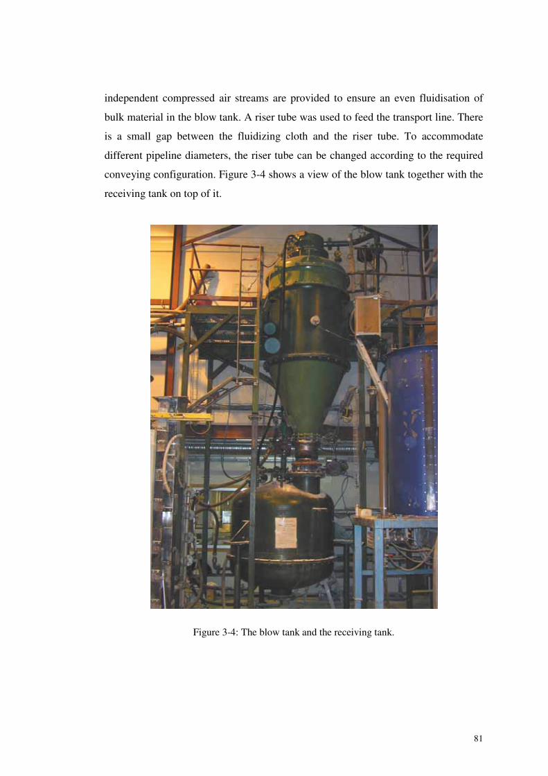
81
independent compressed air streams are provided to ensure an even fluidisation of
bulk material in the blow tank. A riser tube was used to feed the transport line. There
is a small gap between the fluidizing cloth and the riser tube. To accommodate
different pipeline diameters, the riser tube can be changed according to the required
conveying configuration. Figure 3-4 shows a view of the blow tank together with the
receiving tank on top of it.
Figure 3-4: The blow tank and the receiving tank.
82
3.11 Pipelines
The test setup consists of a number of pipes of different diameters and lengths. The
available pipe sizes are 38.5mm, 54mm, 76mm, 106mm and 125mm. The lengths of
the conveying lines can be adjusted according to the requirements of the tests. The
total lengths of available pipelines of different diameters are approximately 500m
each. The experimental setup is also provided with some vertical pipe sections.
Currently, a vertical riser of approximately 8m is possible. The pipelines are laid out
in such a way that it is possible to have any combination of horizontal, inclined and
vertical sections depending upon requirements.
In addition to the straight pipe sections, number of different bends is also available to
use in the conveying loop to meet the objectives of the experiments. Bends of
different radii and configurations like standard 90º, blind tee, etc., provides a great
flexibility to the experimental setup. A part of the full scale pneumatic conveying
pipeline, which lies along the wall of the POSTEC powder laboratory is shown in
Figure 3-5.
Figure 3-5: A part of the conveying pipeline.
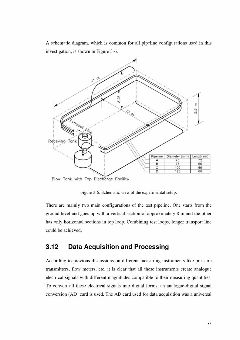
83
A schematic diagram, which is common for all pipeline configurations used in this
investigation, is shown in Figure 3-6.
Figure 3-6: Schematic view of the experimental setup.
There are mainly two main configurations of the test pipeline. One starts from the
ground level and goes up with a vertical section of approximately 8 m and the other
has only horizontal sections in top loop. Combining test loops, longer transport line
could be achieved.
3.12 Data Acquisition and Processing
According to previous discussions on different measuring instruments like pressure
transmitters, flow meters, etc, it is clear that all these instruments create analogue
electrical signals with different magnitudes compatible to their measuring quantities.
To convert all these electrical signals into digital forms, an analogue-digital signal
conversion (AD) card is used. The AD card used for data acquisition was a universal
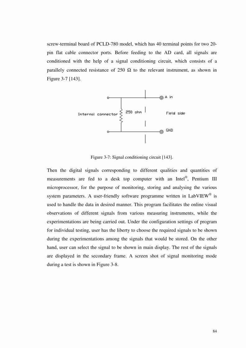
84
screw-terminal board of PCLD-780 model, which has 40 terminal points for two 20-
pin flat cable connector ports. Before feeding to the AD card, all signals are
conditioned with the help of a signal conditioning circuit, which consists of a
parallely connected resistance of 250 Ω to the relevant instrument, as shown in
Figure 3-7 [143].
Figure 3-7: Signal conditioning circuit [143].
Then the digital signals corresponding to different qualities and quantities of
measurements are fed to a desk top computer with an Intel®, Pentium III
microprocessor, for the purpose of monitoring, storing and analysing the various
system parameters. A user-friendly software programme written in LabVIEW® is
used to handle the data in desired manner. This program facilitates the online visual
observations of different signals from various measuring instruments, while the
experimentations are being carried out. Under the configuration settings of program
for individual testing, user has the liberty to choose the required signals to be shown
during the experimentations among the signals that would be stored. On the other
hand, user can select the signal to be shown in main display. The rest of the signals
are displayed in the secondary frame. A screen shot of signal monitoring mode
during a test is shown in Figure 3-8.
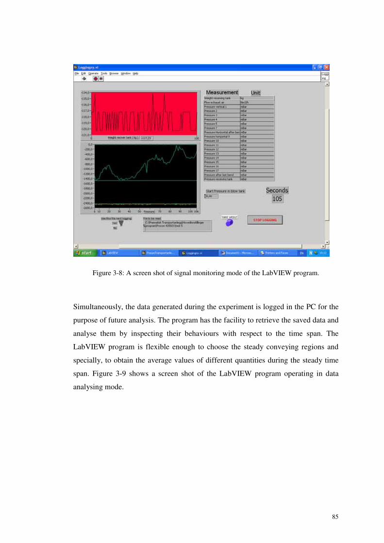
85
Figure 3-8: A screen shot of signal monitoring mode of the LabVIEW program.
Simultaneously, the data generated during the experiment is logged in the PC for the
purpose of future analysis. The program has the facility to retrieve the saved data and
analyse them by inspecting their behaviours with respect to the time span. The
LabVIEW program is flexible enough to choose the steady conveying regions and
specially, to obtain the average values of different quantities during the steady time
span. Figure 3-9 shows a screen shot of the LabVIEW program operating in data
analysing mode.
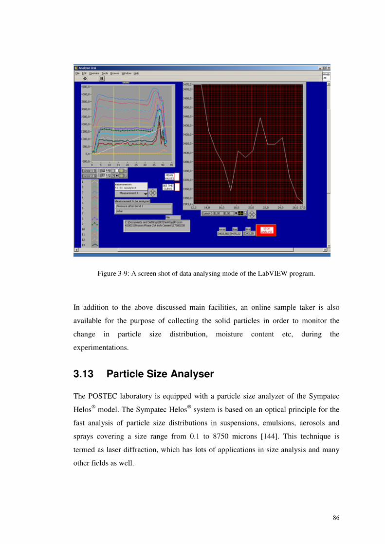
86
Figure 3-9: A screen shot of data analysing mode of the LabVIEW program.
In addition to the above discussed main facilities, an online sample taker is also
available for the purpose of collecting the solid particles in order to monitor the
change in particle size distribution, moisture content etc, during the
experimentations.
3.13 Particle Size Analyser
The POSTEC laboratory is equipped with a particle size analyzer of the Sympatec
Helos® model. The Sympatec Helos® system is based on an optical principle for the
fast analysis of particle size distributions in suspensions, emulsions, aerosols and
sprays covering a size range from 0.1 to 8750 microns [144]. This technique is
termed as laser diffraction, which has lots of applications in size analysis and many
other fields as well.
87
4 PRESSURE DROP DETERMINATION ANDSCALE UP TECHNIQUE
4.1 Introduction
As discussed in the Chapter 1 and 2, pneumatic conveying has been identified as one
of the efficient methods for transporting bulk particulate materials. To ensure reliable
operation of a pneumatic conveying system, at least two parameters have to be
determined accurately in its design stage. These are;
• the pressure head required to have a predetermined solid transport rate along
a known pipeline length, and
• the optimised air velocity to have a safe transport without pipe blockages and
undesirable product degradations/ pipe erosions.
Consequently, plant designers and researchers have been trying to figure out a
straight forward, easy but reliable method to determine these parameters using
physical and geometrical characteristics of the conveying pipeline and bulk material
to be transported in it.
The strong dependence of the possible mode of pneumatic transport on the nature of
the material to be conveyed plays a significant role in the design of a pneumatic
conveying system. Unfortunately, there exists no reliable technique for
characterisation of particulate materials, which can be readily used for the design of
pneumatic conveying systems as available in the open literature. Consequently, the
system designers are compelled to use experimentation based design strategies in the
design of industrial pneumatic conveying installations.
In this approach, a representative sample of product, which is to be conveyed in the
industrial plant, is tested in a laboratory pneumatic conveying test rig (pilot plant)
over a wide range of operating conditions. The product and airflow rates and
resulting pressure drops are measured. Additionally, the minimum conveying
conditions and blocking limits are also observed. This approach has the advantage
that real test data on the product to be conveyed in the proposed system are used for
88
the design process. Thus, it gives a high reliability level about the effects of product
type. This is very important because it provides useful information on the
conveyability of product. On the other hand, in determination of specified conveying
limits like minimum conveying velocity, pressure minimum conveying, etc, this
approach gives better results.
However, it is not always feasible to use a pilot plant, which is of identical geometry
with respect to length, pipe bore, number of bends, types of bends, etc., to that of the
required industrial installation. Therefore, it is required to scale up the conveying
characteristics based on the pilot plant data, to predict the behaviour of the proposed
industrial (full scale) plant, using some experimentally determined factors. Scaling
up in terms of pipe line geometry needs to be carried out with respect to conveying
distance, pipeline bore and the air supply pressure available. Pipeline material, bend
geometry and stepped pipelines are other important parameters that need to be
considered. The scaling up of pilot plant data is considered to be the most important
stage of the design process, because it provides the required link between laboratory
pilot plant apparatus and the full-scale industrial installation. Hence, accuracy and
reliability of scaling methodology are vital.
The importance of scaling up methods in pneumatic conveying system designs has
paved the way for quite a large number of research studies on the subject. Many
researchers have been trying out to establish the mathematical models and relevant
conditions of scaling up procedure [16, 22, 25, 42, 95, 97, 101, 145, 146], during the
last two decades or so. In Chapter 2, their applicability and limitations were
discussed in details. Although several relationships, based on different conditions
have been proposed in the literature on scaling concepts, there are still some doubts
and uncertainties about their validity. Under this chapter, the theoretical approach to
the proposed model and the experimental measurements together with the procedure
are discussed in details.
89
4.2 Theoretical Approach
4.2.1 Background
When the published scaling techniques are concerned, there can be seen two basic
approaches:
1. the global testing approach [16, 95, 145]
2. the piecewise approach [22, 25, 42, 101]
In the first approach, the transport pipeline is considered as a whole unit with the
different components like bends, vertical sections, etc, without taking into account
their discrete positions on the pipeline. In most of the applications of this method, the
equivalent length approach is used to address the different components despite their
different position either in pilot plant or in projected plant. Alternatively, the
individual features of the pipeline are treated separately in the piecewise approach.
The different components on the transport line like bends, vertical sections, etc, of
the pilot plant are considered separately and different models are formulated using
the experimentally measured values of pressure drop across them. Then, in the
second stage, those models are used to predict the pipeline pressure drop of the
proposed plant, starting from a known flow condition at one end of the pipeline and
estimating the pressure drop and change in flow conditions caused by each
component and straight length in turn, processing right along the pipeline and thus
finishing up with a value for the total pressure drop. These approaches have their
own advantages and limitations, which were discussed in the Section 2.9.
The determination of the pressure drop in single-phase flow situation is well
established with more reliable mathematical models such as French engineer Henry
Darcy’s [44]. There is a quite long history of Darcy’s equation, which is also defined
with different terminologies like Darcy-Weisbach’s equation, Fanning’s theory, etc.
An excellent survey on the historical development of Darcy-Weisbach equation and
the contributions made by other research workers and scientists to establish it as a
universally acceptable theory, could be seen in Ref. [147] and [148].
90
However, Darcy’s equation could be represented in the simplest way as shown in
Equation (4.1).
2
42
af v LP
D
ρΔ = (4.1)
In later developments, some researchers tried to modify Darcy’s theory to suit
multiphase flow situations. The applications of such attempts could also be seen in
research publications on pneumatic conveying. Some researchers [16, 22, 25, 42, 46,
95] have used this equation as a basis for models, which could be used to calculate
the total pipeline pressure drop of pneumatic conveying systems. Most of them have
tried to split the effect of friction caused by the gas-solid mixture into two
components as air friction and solid contribution to it. This approach leads to create
two hypothetical pressure drop components namely; air only pressure drop and
pressure drop due to the presence of solid particles, as shown in equation (4.2), (4.3)
and (4.4).
T a sp p pΔ = Δ + Δ (4.2)
2
2a a a
Lp v
Dλ ρΔ = (4.3)
2
2s s a
Lp v
Dμλ ρΔ = (4.4)
In this approach, calculation of air only pressure drop using the Equation (4.3) gives
quite a straightforward methodology, which is similar to the conventional single
phase flow situation, where as some additional terms and modifications are
introduced in case of solid pressure drop. One of the modifications is to replace the
air friction factor with its counterpart relevant to solid particles, namely; solid
friction factor (�s), as shown in the Equation (4.4). But, unfortunately, this concept of
‘solid friction factor’ has not yet been established as a universally accepted
parameter and thus a lot of divergent opinions could be found in literature [22, 26,
41, 43, 53, 77, 78, 92, 149]. Under Chapter 2, Table 2.2 shows some of the available
correlations for determining the solid friction factor. One can clearly see how they
vary from one another. On the other hand, some models [41, 43, 77, 92] even require
solid velocity, which would be rather difficult to determine in dense phase conveying
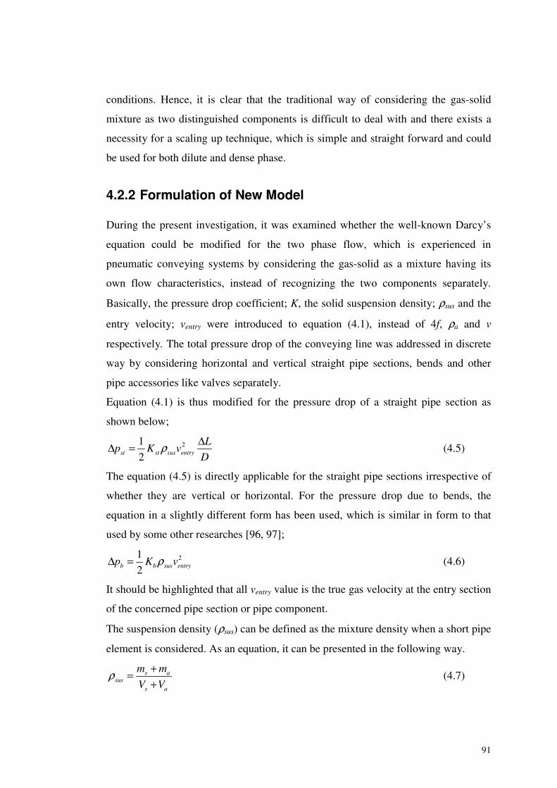
91
conditions. Hence, it is clear that the traditional way of considering the gas-solid
mixture as two distinguished components is difficult to deal with and there exists a
necessity for a scaling up technique, which is simple and straight forward and could
be used for both dilute and dense phase.
4.2.2 Formulation of New Model
During the present investigation, it was examined whether the well-known Darcy’s
equation could be modified for the two phase flow, which is experienced in
pneumatic conveying systems by considering the gas-solid as a mixture having its
own flow characteristics, instead of recognizing the two components separately.
Basically, the pressure drop coefficient; K, the solid suspension density; ρsus and the
entry velocity; ventry were introduced to equation (4.1), instead of 4f, ρa and v
respectively. The total pressure drop of the conveying line was addressed in discrete
way by considering horizontal and vertical straight pipe sections, bends and other
pipe accessories like valves separately.
Equation (4.1) is thus modified for the pressure drop of a straight pipe section as
shown below;
21
2st st sus entry
Lp K v
Dρ ΔΔ = (4.5)
The equation (4.5) is directly applicable for the straight pipe sections irrespective of
whether they are vertical or horizontal. For the pressure drop due to bends, the
equation in a slightly different form has been used, which is similar in form to that
used by some other researches [96, 97];
21
2b b sus entryp K vρΔ = (4.6)
It should be highlighted that all ventry value is the true gas velocity at the entry section
of the concerned pipe section or pipe component.
The suspension density (ρsus) can be defined as the mixture density when a short pipe
element is considered. As an equation, it can be presented in the following way.
s asus
s a
m m
V Vρ +=
+(4.7)
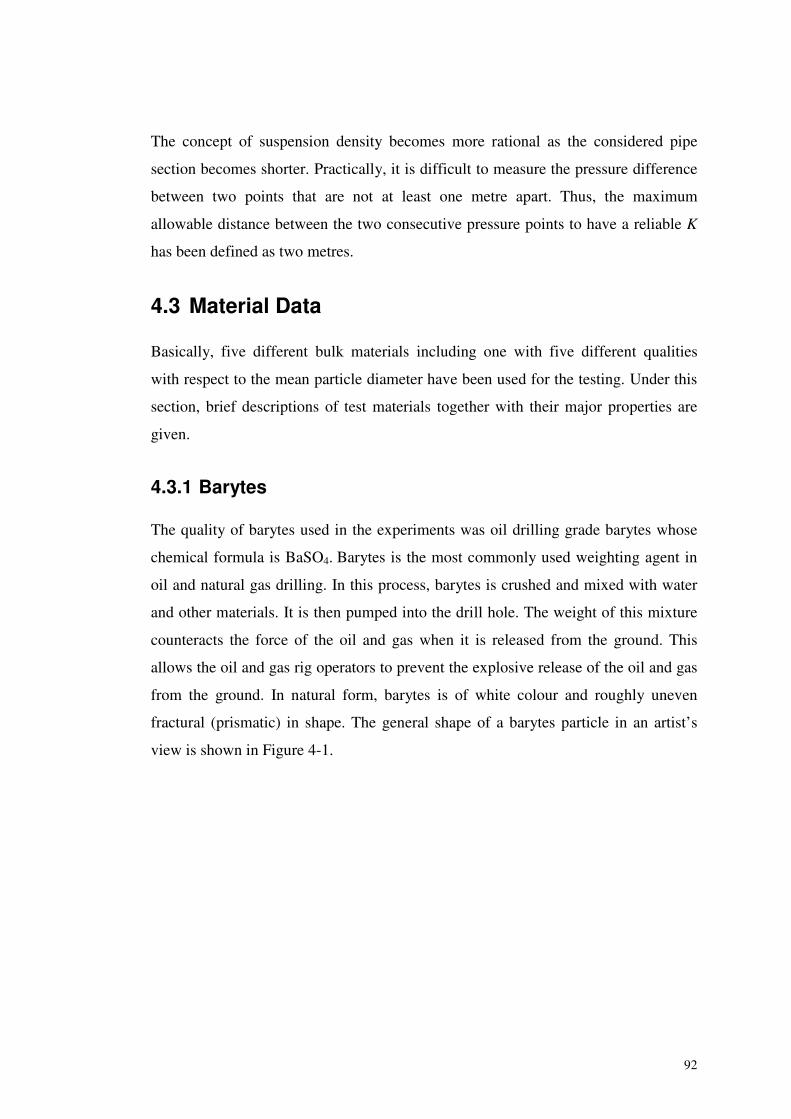
92
The concept of suspension density becomes more rational as the considered pipe
section becomes shorter. Practically, it is difficult to measure the pressure difference
between two points that are not at least one metre apart. Thus, the maximum
allowable distance between the two consecutive pressure points to have a reliable K
has been defined as two metres.
4.3 Material Data
Basically, five different bulk materials including one with five different qualities
with respect to the mean particle diameter have been used for the testing. Under this
section, brief descriptions of test materials together with their major properties are
given.
4.3.1 Barytes
The quality of barytes used in the experiments was oil drilling grade barytes whose
chemical formula is BaSO4. Barytes is the most commonly used weighting agent in
oil and natural gas drilling. In this process, barytes is crushed and mixed with water
and other materials. It is then pumped into the drill hole. The weight of this mixture
counteracts the force of the oil and gas when it is released from the ground. This
allows the oil and gas rig operators to prevent the explosive release of the oil and gas
from the ground. In natural form, barytes is of white colour and roughly uneven
fractural (prismatic) in shape. The general shape of a barytes particle in an artist’s
view is shown in Figure 4-1.
93
Figure 4-1: The shape of a barytes particle in an artist’s view [150].
4.3.2 Bentonite
Bentonite is used in preparation of drilling mud and it is mainly used as circulation
mud in rotary system of drilling for oil. The main purpose of bentonite is to lubricate
and cool the rotary cutting bits, carry away rock cutting fragments and to act as a seal
against the escape of gas from the bore hole and to improve and prevent the hole
from blowing out. Another function of such bentonite based fluids is to condition the
wall of the drill hole to prevent caving. The chemical formula of bentonite is
generally given as Al2O34SiO2H2O and bentonite particles are of light cream in
colour.
4.3.3 Cement
The tested quality of cement is called as oil well cement because of it’s usage in the
oil and gas industry. It has the characteristics of high sulphate resistance and is
usually used for the cementing operations related in oil drilling sites. Cementing is a
very important phase of the well construction plan. Usually, an oil well is created by
drilling a hole (5 to 30 inches wide) into the earth with an oil rig turning a drill bit.
After the hole is drilled, a metal pipe called 'casing' is cemented into the hole. During
94
this process the casing is reciprocated or rotated to allow the scratches to work to
remove excess wall cake to give the cement a better bond.
4.3.4 Ilmenite
This is also related to the oil well drilling. Ilmenite (FeTiO3 –Iron Titanium Oxide) is
also used as a weighting agent instead of barytes. In natural form ilmenite is of
colour Iron black or black and conchoidal in shape as shown in Figure 4-2.
Figure 4-2: An ilmenite particle under microscope [151].
4.3.5 Alumina
Alumina has a chemical formula of Al2O3 and is a compound of aluminium and
oxygen. Alumina qualities used for the testing are used in the aluminium industry.
Usually, alumina is refined from the chemical breakdown of bauxite and it is the
starting material for the extraction of aluminium by means of the electrolytic
reduction process. Aluminium oxide, commonly referred to as alumina, possesses
strong ionic inter-atomic bonding giving rise to its desirable material characteristics.
It can exist in several crystalline phases, which all revert to the most stable hexagonal
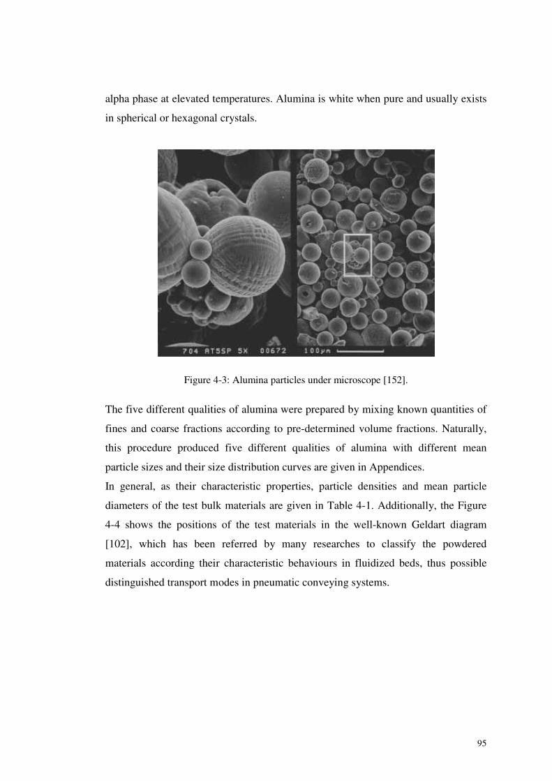
95
alpha phase at elevated temperatures. Alumina is white when pure and usually exists
in spherical or hexagonal crystals.
Figure 4-3: Alumina particles under microscope [152].
The five different qualities of alumina were prepared by mixing known quantities of
fines and coarse fractions according to pre-determined volume fractions. Naturally,
this procedure produced five different qualities of alumina with different mean
particle sizes and their size distribution curves are given in Appendices.
In general, as their characteristic properties, particle densities and mean particle
diameters of the test bulk materials are given in Table 4-1. Additionally, the Figure
4-4 shows the positions of the test materials in the well-known Geldart diagram
[102], which has been referred by many researches to classify the powdered
materials according their characteristic behaviours in fluidized beds, thus possible
distinguished transport modes in pneumatic conveying systems.
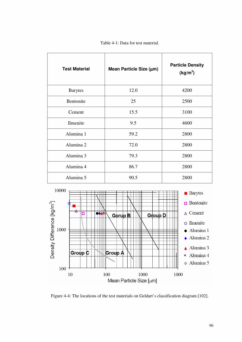
96
Table 4-1: Data for test material.
Test Material Mean Particle Size (μμμμm)Particle Density
(kg/m3)
Barytes 12.0 4200
Bentonite 25 2500
Cement 15.5 3100
Ilmenite 9.5 4600
Alumina 1 59.2 2800
Alumina 2 72.0 2800
Alumina 3 79.3 2800
Alumina 4 86.7 2800
Alumina 5 90.5 2800
Figure 4-4: The locations of the test materials on Geldart’s classification diagram [102].
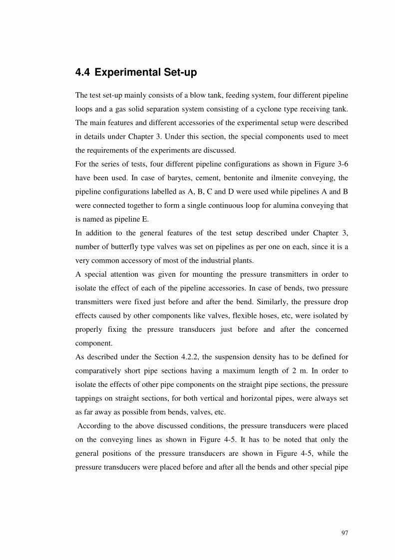
97
4.4 Experimental Set-up
The test set-up mainly consists of a blow tank, feeding system, four different pipeline
loops and a gas solid separation system consisting of a cyclone type receiving tank.
The main features and different accessories of the experimental setup were described
in details under Chapter 3. Under this section, the special components used to meet
the requirements of the experiments are discussed.
For the series of tests, four different pipeline configurations as shown in Figure 3-6
have been used. In case of barytes, cement, bentonite and ilmenite conveying, the
pipeline configurations labelled as A, B, C and D were used while pipelines A and B
were connected together to form a single continuous loop for alumina conveying that
is named as pipeline E.
In addition to the general features of the test setup described under Chapter 3,
number of butterfly type valves was set on pipelines as per one on each, since it is a
very common accessory of most of the industrial plants.
A special attention was given for mounting the pressure transmitters in order to
isolate the effect of each of the pipeline accessories. In case of bends, two pressure
transmitters were fixed just before and after the bend. Similarly, the pressure drop
effects caused by other components like valves, flexible hoses, etc, were isolated by
properly fixing the pressure transducers just before and after the concerned
component.
As described under the Section 4.2.2, the suspension density has to be defined for
comparatively short pipe sections having a maximum length of 2 m. In order to
isolate the effects of other pipe components on the straight pipe sections, the pressure
tappings on straight sections, for both vertical and horizontal pipes, were always set
as far away as possible from bends, valves, etc.
According to the above discussed conditions, the pressure transducers were placed
on the conveying lines as shown in Figure 4-5. It has to be noted that only the
general positions of the pressure transducers are shown in Figure 4-5, while the
pressure transducers were placed before and after all the bends and other special pipe
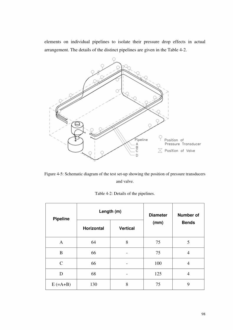
98
elements on individual pipelines to isolate their pressure drop effects in actual
arrangement. The details of the distinct pipelines are given in the Table 4-2.
Figure 4-5: Schematic diagram of the test set-up showing the position of pressure transducers
and valve.
Table 4-2: Details of the pipelines.
Length (m)
Pipeline
Horizontal Vertical
Diameter
(mm)
Number of
Bends
A 64 8 75 5
B 66 - 75 4
C 66 - 100 4
D 68 - 125 4
E (=A+B) 130 8 75 9
99
4.5 Experimental Procedure
For the investigation, five different materials including one with five different
qualities (Table 4-1) have been used to test with five different pipeline configurations
(Figure 4-5 and Table 4-2). For each material, the number of test runs has been
carried out by varying the start pressure (set pressure of blow tank) and the
volumetric flow rate of conveying air. The test procedures adopted for the different
bulk materials and pipeline configurations were similar to each other. The whole
experimental procedure can be described by dividing it basically into three main
sections; i.e., pre-test arrangements, testing procedure and post-test analysis. Setting
up of test rig, programming of data acquisition software, etc, come under the pre-test
arrangements, while post-test analysis comprises of test data averaging and relevant
analysis. The general procedure of experiments is explained in detail in the following
section while the special conditions for particular materials are indicated in case by
case basis.
For each test, approximately 0.5 - 1.0 m3 of bulk material was used for testing.
Before testing in the pneumatic conveying rig, a representative sample of each
material was tested in the laboratory for the size distribution. During testing samples
were collected from time to time using an online sampler and size analysis was
carried out in order to check if there were any size degradation during transportation.
The first step of testing was filling up the blow tank with the test material. Before
pressurising the blow tank, the pressure control valve on the main air supply line
(PCV1 in Figure 3-1) was regulated by setting the pre-determined pressure value on
the pressure control unit. Generally, the pre-set pressure values were ranging from 2
bar to 5.5 bar in 0.5 bar intervals. For higher pipe sizes (e.g. 125 mm), this value has
to be lowered to 1.75 bar. By opening the main air supply valve, the blow tank was
allowed to pressurise gradually. In this stage, the valves on the fluidising air supply
side (V6, V8, V10 and V12 in Figure 3-1) were partially opened to make sure of
even fluidisation.
After the pressure in the blow tank reached to the desired value, the conveying of
material was started by opening the main supply valve on conveying line (V16 in
100
Figure 3-1) and the data acquisition programme was simultaneously started. The
recording of all signals were inspected during the test run. During the comparatively
long conveying cycles, the settings of the fluidisation air supply valves were changed
in order to get different air volume flow rate values within one cycle. In case of
smaller pipe sizes, it could be possible to obtain 3-4 different stable conveying
regions with respect to the air volume flow rate, depending on the cycle time. The
samples were taken using online sampler at regular intervals of approximately 15
runs and were tested in the laboratory for particle size distribution in order to check if
any size degradation had occurred.
The end of the conveying cycle could be determined by checking the amount of
material collected in the receiving tank that was digitally displayed on an LCD panel
in main control panel. Then, the main supply valve of material was closed and the
data logging programme was also stopped at the same time. The pipeline was then
supplied some additional compressed air through the by-pass line to clean any
residual materials deposited inside the pipeline. After that, the blow tank was let to
depressurise through the ventilation line provided in between the blow and the
receiving tank. Then, the materials were taken down to the blow tank for the next test
run.
The different signals recorded during the test were then analysed and the stable
conveying regions were identified by inspecting the signal curves with respect to
time scale. One typical set of signal curves are shown in Figure 4-6.
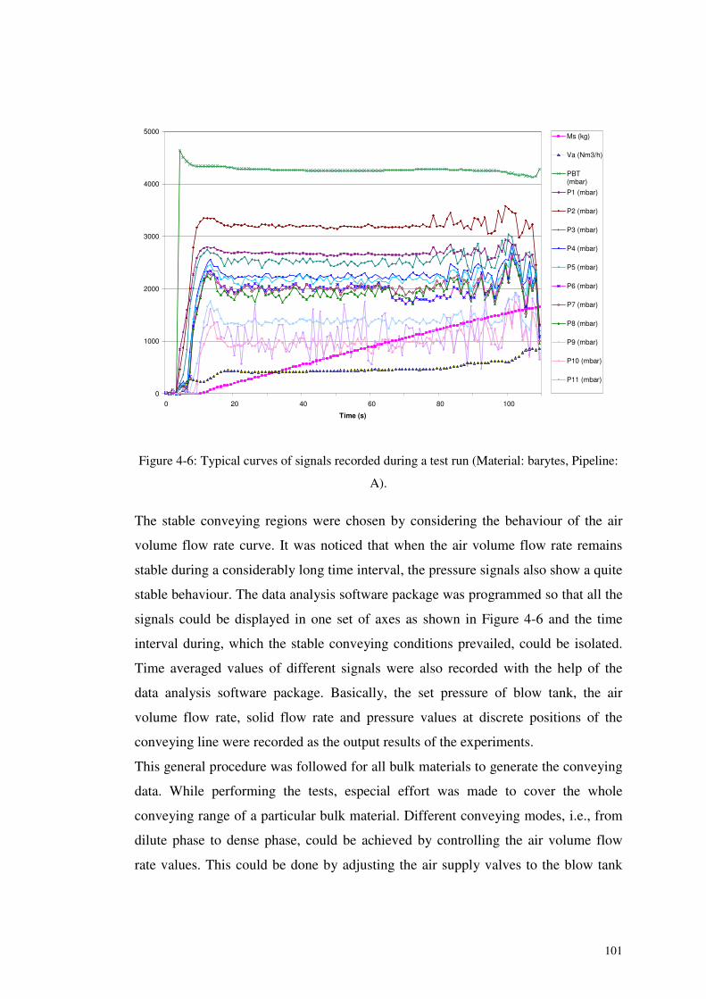
101
0
1000
2000
3000
4000
5000
0 20 40 60 80 100
Time (s)
Ms (kg)
Va (Nm3/h)
PBT(mbar)
P1 (mbar)
P2 (mbar)
P3 (mbar)
P4 (mbar)
P5 (mbar)
P6 (mbar)
P7 (mbar)
P8 (mbar)
P9 (mbar)
P10 (mbar)
P11 (mbar)
Figure 4-6: Typical curves of signals recorded during a test run (Material: barytes, Pipeline:
A).
The stable conveying regions were chosen by considering the behaviour of the air
volume flow rate curve. It was noticed that when the air volume flow rate remains
stable during a considerably long time interval, the pressure signals also show a quite
stable behaviour. The data analysis software package was programmed so that all the
signals could be displayed in one set of axes as shown in Figure 4-6 and the time
interval during, which the stable conveying conditions prevailed, could be isolated.
Time averaged values of different signals were also recorded with the help of the
data analysis software package. Basically, the set pressure of blow tank, the air
volume flow rate, solid flow rate and pressure values at discrete positions of the
conveying line were recorded as the output results of the experiments.
This general procedure was followed for all bulk materials to generate the conveying
data. While performing the tests, especial effort was made to cover the whole
conveying range of a particular bulk material. Different conveying modes, i.e., from
dilute phase to dense phase, could be achieved by controlling the air volume flow
rate values. This could be done by adjusting the air supply valves to the blow tank
102
manually. From an intermediate value, the air flow rate was increased gradually to
very high values where very dilute phase conveying prevailed. On the other hand, the
air flow was gradually decreased until it reached to the total pipeline blockage. This
procedure was repeated until it generated a large number of data points, which were
satisfactorily enough to generate the pneumatic conveying characteristic curves. The
conveying characteristics curves in terms of air volume flow rate, solid mass flow
rate and pipeline pressure drop were generated at the same time as the tests
proceeded.
4.6 Experimental Results
The results of the experimentations are discussed in a few stages. Initially, the
conveying characteristics curves of different materials will be discussed. The special
behaviours of different materials were analysed next and the results relevant to the
scaling model will be discussed at the end.
4.6.1 Pneumatic Conveying Characteristics Curves
Under the Section 1.8, the concept and the importance of pneumatic conveying
characteristics of a bulk material in a system design was explained in details. With
the test results, pneumatic conveying characteristics curves were developed for the
various combinations of different materials and different pipeline configurations. In
this section, some of those characteristics curves, which represent the all test
materials and pipeline configurations, are presented and their special features are
discussed. The rest of the conveying characteristics are given in Appendices. The
nomenclatures indicated in the Figures are as depicted in Figure 3-6.
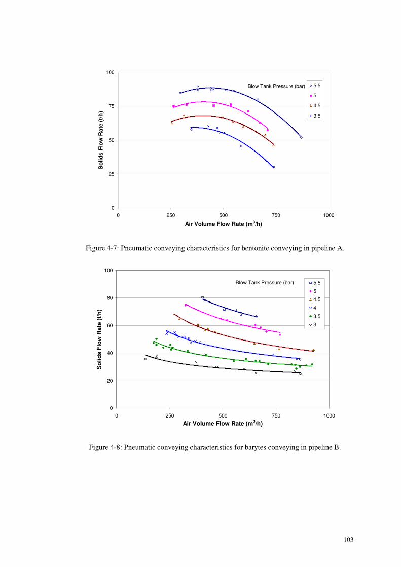
103
0
25
50
75
100
0 250 500 750 1000
Air Volume Flow Rate (m3/h)
So
lids
Flo
wR
ate
(t/h
)
5.5
5
4.5
3.5
Blow Tank Pressure (bar)
Figure 4-7: Pneumatic conveying characteristics for bentonite conveying in pipeline A.
0
20
40
60
80
100
0 250 500 750 1000
Air Volume Flow Rate (m3/h)
So
lids
Flo
wR
ate
(t/h
)
5,5
5
4.5
4
3.5
3
Blow Tank Pressure (bar)
Figure 4-8: Pneumatic conveying characteristics for barytes conveying in pipeline B.
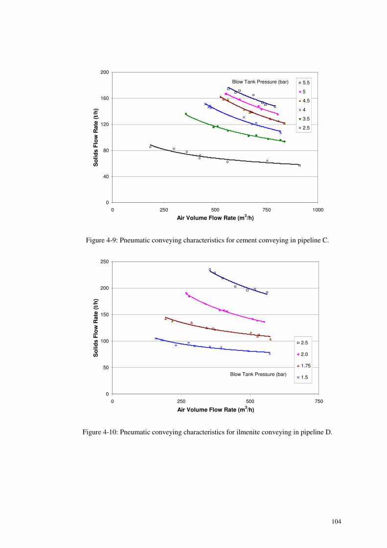
104
0
40
80
120
160
200
0 250 500 750 1000
Air Volume Flow Rate (m3/h)
So
lids
Flo
wR
ate
(t/h
)
5.5
5
4.5
4
3.5
2.5
Blow Tank Pressure (bar)
Figure 4-9: Pneumatic conveying characteristics for cement conveying in pipeline C.
0
50
100
150
200
250
0 250 500 750
Air Volume Flow Rate (m3/h)
So
lids
Flo
wR
ate
(t/h
)
2.5
2.0
1.75
1.5Blow Tank Pressure (bar)
Figure 4-10: Pneumatic conveying characteristics for ilmenite conveying in pipeline D.
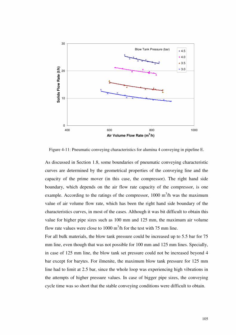
105
0
10
20
30
400 600 800 1000
Air Volume Flow Rate (m3/h)
So
lids
Flo
wR
ate
(t/h
)
4.5
4.0
3.5
3.0
Blow Tank Pressure (bar)
Figure 4-11: Pneumatic conveying characteristics for alumina 4 conveying in pipeline E.
As discussed in Section 1.8, some boundaries of pneumatic conveying characteristic
curves are determined by the geometrical properties of the conveying line and the
capacity of the prime mover (in this case, the compressor). The right hand side
boundary, which depends on the air flow rate capacity of the compressor, is one
example. According to the ratings of the compressor, 1000 m3/h was the maximum
value of air volume flow rate, which has been the right hand side boundary of the
characteristics curves, in most of the cases. Although it was bit difficult to obtain this
value for higher pipe sizes such as 100 mm and 125 mm, the maximum air volume
flow rate values were close to 1000 m3/h for the test with 75 mm line.
For all bulk materials, the blow tank pressure could be increased up to 5.5 bar for 75
mm line, even though that was not possible for 100 mm and 125 mm lines. Specially,
in case of 125 mm line, the blow tank set pressure could not be increased beyond 4
bar except for barytes. For ilmenite, the maximum blow tank pressure for 125 mm
line had to limit at 2.5 bar, since the whole loop was experiencing high vibrations in
the attempts of higher pressure values. In case of bigger pipe sizes, the conveying
cycle time was so short that the stable conveying conditions were difficult to obtain.
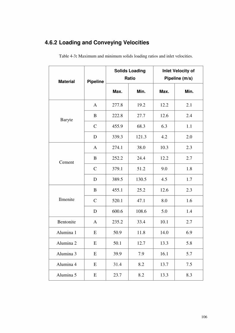
106
4.6.2 Loading and Conveying Velocities
Table 4-3: Maximum and minimum solids loading ratios and inlet velocities.
Solids Loading
Ratio
Inlet Velocity of
Pipeline (m/s)Material Pipeline
Max. Min. Max. Min.
A 277.8 19.2 12.2 2.1
B 222.8 27.7 12.6 2.4
C 455.9 68.3 6.3 1.1Baryte
D 339.3 121.3 4.2 2.0
A 274.1 38.0 10.3 2.3
B 252.2 24.4 12.2 2.7
C 379.1 51.2 9.0 1.8Cement
D 389.5 130.5 4.5 1.7
B 455.1 25.2 12.6 2.3
C 520.1 47.1 8.0 1.6Ilmenite
D 600.6 108.6 5.0 1.4
Bentonite A 235.2 33.4 10.1 2.7
Alumina 1 E 50.9 11.8 14.0 6.9
Alumina 2 E 50.1 12.7 13.3 5.8
Alumina 3 E 39.9 7.9 16.1 5.7
Alumina 4 E 31.4 8.2 13.7 7.5
Alumina 5 E 23.7 8.2 13.3 8.3
107
Table 4-3 shows the maximum and minimum values of solids loading ratios and
conveying velocities achieved for different combinations of conveying bulk material
and pipeline configurations. Accordingly, the maximum loading ratios of all
materials except alumina were in the range of 200-600, while that of alumina
qualities were in range of 30-50. Another feature was the comparatively high values
of conveying velocity processed by alumina. In most of the cases, barytes, cement,
bentonite and ilmenite could convey with the minimum velocity of 2 m/s
approximately, whereas the minimum velocity was approximately 7 m/s for alumina.
The clear difference of the conveying figures in terms of loadings and velocities can
be explained with the help of conveying distances. As shown in Figure 4-5 and Table
4-2, it is clear that conveying distance of barytes, cement, bentonite and ilmenite was
shorter than that of alumina. The conveying distance of alumina qualities was
approximately double of the other cases. According to findings of many researchers
[6, 16, 20, 27], there is a reciprocal relationship between the solid mass flow rate and
the conveying distance. This may be one of the reasons for the differences in solid
loadings and velocities revealed in the testing.
4.7 Variations of ‘K’ Curves
After obtaining the required data, the pressure drop values across the vertical and
horizontal straight sections and bends were considered and relevant K values were
calculated according to the conditions discussed under Section 4.2.2. Under this sub-
section, the procedure followed to obtain the K curves and the individual
characteristic features of K curves of different materials and of different pipeline
components are discussed in detail. The effect of the orientation of pipe section is
also discussed with respect to the different conveying material. At the end, the
characteristic features of combined K curves are analysed.
4.7.1 Method of ‘K’ Calculation
As discussed under the Section 4.2.2, the K values for different pipe sections were
calculated with the help of Equations (4.5) and (4.6). The experimental pressure
108
readings of pressure transducers fixed before and after the concerned section were
used to determine the pressure drop of the same. To calculate the air velocity and
volume flow rate at the entry section, the effect of compressibility had to be
considered. The true values of above parameters were determined by adjusting the
experimentally measured air volume flow rate according to the true pressure value
prevailing at the entrance of the pipe section. In the same line, the mass flow rate of
air was also determined. The time averaged value of solids mass flow rate, during
which the stable conveying conditions were prevailed was used to determine the
mass and volume flow rate of solids within the concerned section. Using Equation
(4.7), the suspension densities of considered sections were calculated. Finally, the
value of K was calculated using Equation (4.5) or Equation (4.6). Figure 4-12 shows
a general procedure adopted to calculate K for different section as a flow chart.
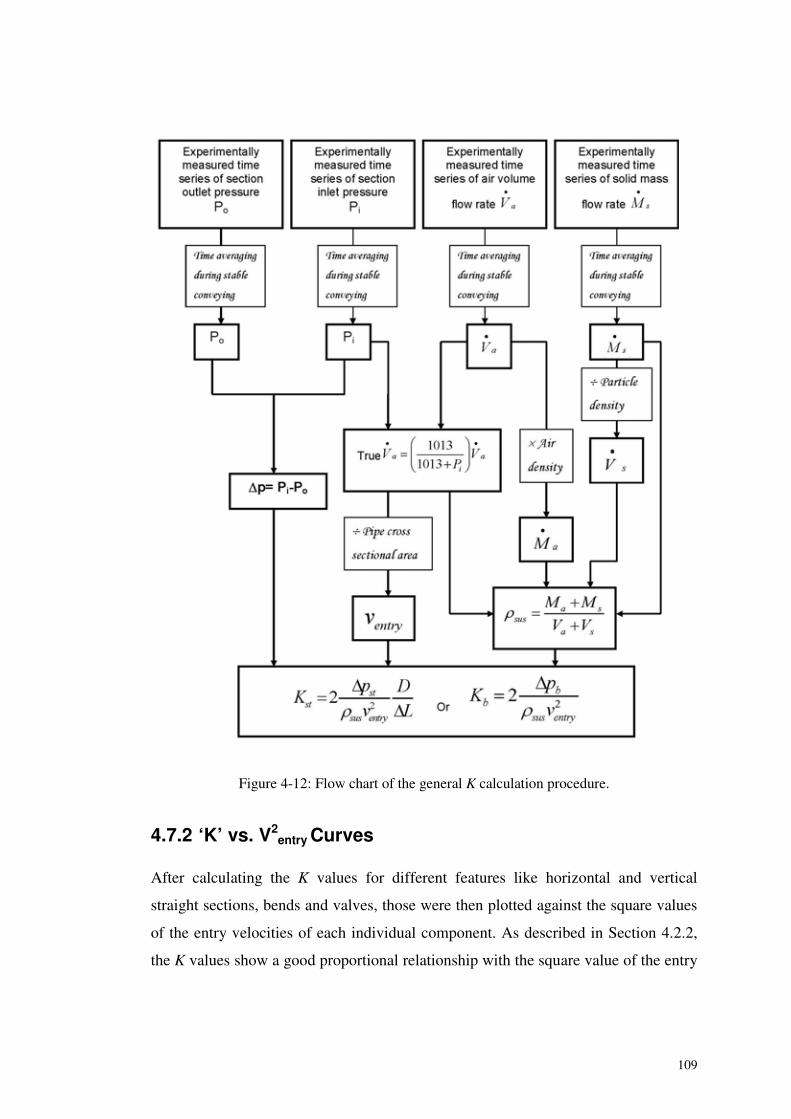
109
Figure 4-12: Flow chart of the general K calculation procedure.
4.7.2 ‘K’ vs. V2entry Curves
After calculating the K values for different features like horizontal and vertical
straight sections, bends and valves, those were then plotted against the square values
of the entry velocities of each individual component. As described in Section 4.2.2,
the K values show a good proportional relationship with the square value of the entry
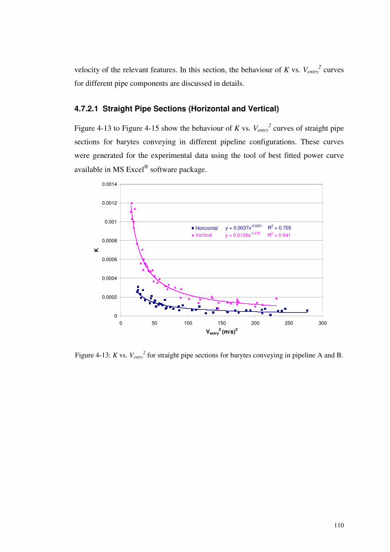
110
velocity of the relevant features. In this section, the behaviour of K vs. Ventry2 curves
for different pipe components are discussed in details.
4.7.2.1 Straight Pipe Sections (Horizontal and Vertical)
Figure 4-13 to Figure 4-15 show the behaviour of K vs. Ventry2 curves of straight pipe
sections for barytes conveying in different pipeline configurations. These curves
were generated for the experimental data using the tool of best fitted power curve
available in MS Excel® software package.
y = 0.0126x-0.875 R2 = 0.941
y = 0.0037x-0.8351 R2 = 0.705
0
0.0002
0.0004
0.0006
0.0008
0.001
0.0012
0.0014
0 50 100 150 200 250 300
Ventry2 (m/s)2
K
HorizontalVertical
Figure 4-13: K vs. Ventry2 for straight pipe sections for barytes conveying in pipeline A and B.
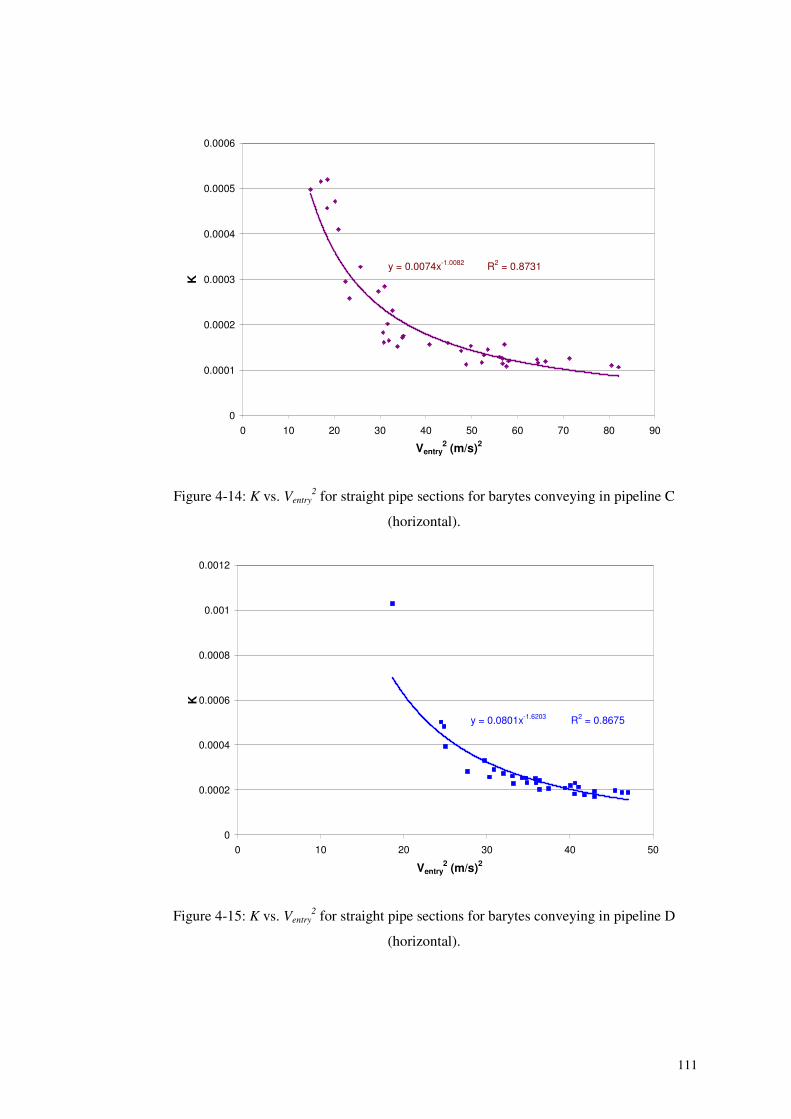
111
y = 0.0074x-1.0082 R2 = 0.8731
0
0.0001
0.0002
0.0003
0.0004
0.0005
0.0006
0 10 20 30 40 50 60 70 80 90
Ventry2 (m/s)2
K
Figure 4-14: K vs. Ventry2 for straight pipe sections for barytes conveying in pipeline C
(horizontal).
y = 0.0801x-1.6203 R2 = 0.8675
0
0.0002
0.0004
0.0006
0.0008
0.001
0.0012
0 10 20 30 40 50
Ventry2 (m/s)2
K
Figure 4-15: K vs. Ventry2 for straight pipe sections for barytes conveying in pipeline D
(horizontal).
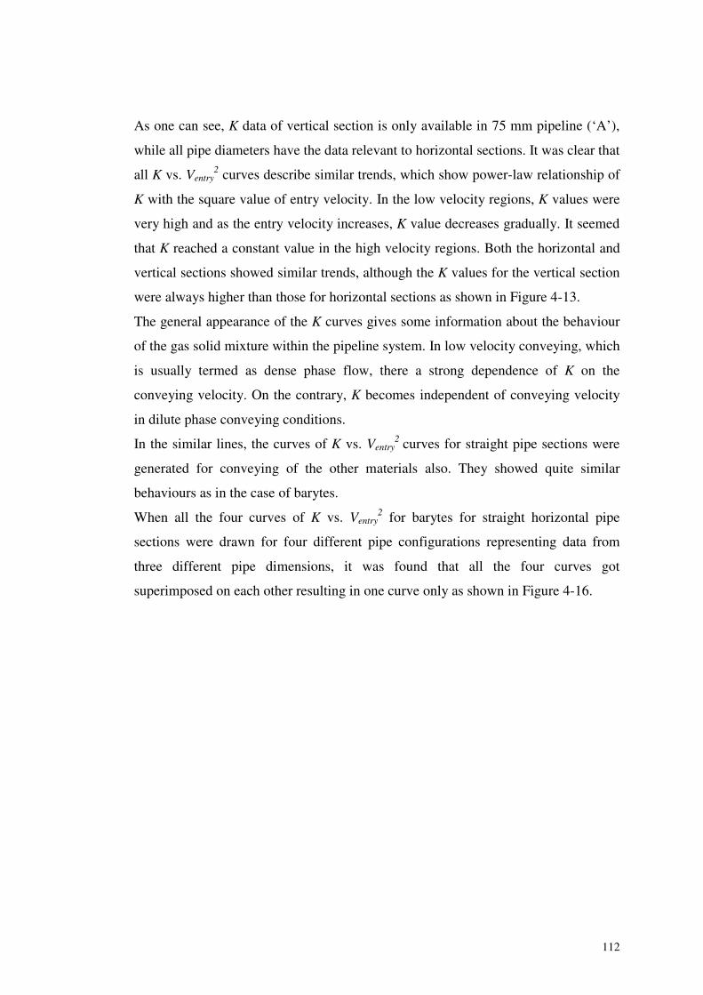
112
As one can see, K data of vertical section is only available in 75 mm pipeline (‘A’),
while all pipe diameters have the data relevant to horizontal sections. It was clear that
all K vs. Ventry2 curves describe similar trends, which show power-law relationship of
K with the square value of entry velocity. In the low velocity regions, K values were
very high and as the entry velocity increases, K value decreases gradually. It seemed
that K reached a constant value in the high velocity regions. Both the horizontal and
vertical sections showed similar trends, although the K values for the vertical section
were always higher than those for horizontal sections as shown in Figure 4-13.
The general appearance of the K curves gives some information about the behaviour
of the gas solid mixture within the pipeline system. In low velocity conveying, which
is usually termed as dense phase flow, there a strong dependence of K on the
conveying velocity. On the contrary, K becomes independent of conveying velocity
in dilute phase conveying conditions.
In the similar lines, the curves of K vs. Ventry2 curves for straight pipe sections were
generated for conveying of the other materials also. They showed quite similar
behaviours as in the case of barytes.
When all the four curves of K vs. Ventry2 for barytes for straight horizontal pipe
sections were drawn for four different pipe configurations representing data from
three different pipe dimensions, it was found that all the four curves got
superimposed on each other resulting in one curve only as shown in Figure 4-16.
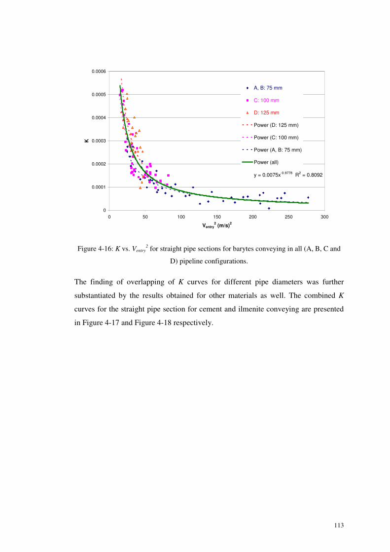
113
y = 0.0075x-0.9778 R2 = 0.8092
0
0.0001
0.0002
0.0003
0.0004
0.0005
0.0006
0 50 100 150 200 250 300
Ventry2 (m/s)2
KA, B: 75 mm
C: 100 mm
D: 125 mm
Power (D: 125 mm)
Power (C: 100 mm)
Power (A, B: 75 mm)
Power (all)
Figure 4-16: K vs. Ventry2 for straight pipe sections for barytes conveying in all (A, B, C and
D) pipeline configurations.
The finding of overlapping of K curves for different pipe diameters was further
substantiated by the results obtained for other materials as well. The combined K
curves for the straight pipe section for cement and ilmenite conveying are presented
in Figure 4-17 and Figure 4-18 respectively.
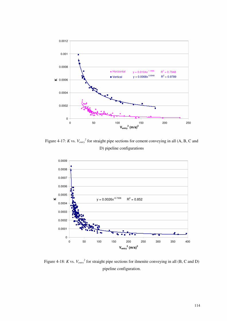
114
y = 0.0104x-1.1866 R2 = 0.7948
y = 0.0068x-0.6948 R2 = 0.9789
0
0.0002
0.0004
0.0006
0.0008
0.001
0.0012
0 50 100 150 200 250
Ventry2 (m/s)2
K
Horizontal
Vertical
Figure 4-17: K vs. Ventry2 for straight pipe sections for cement conveying in all (A, B, C and
D) pipeline configurations
y = 0.0026x-0.7336 R2 = 0.852
0
0.0001
0.0002
0.0003
0.0004
0.0005
0.0006
0.0007
0.0008
0.0009
0 50 100 150 200 250 300 350 400
Ventry2 (m/s)2
K
Figure 4-18: K vs. Ventry2 for straight pipe sections for ilmenite conveying in all (B, C and D)
pipeline configuration.
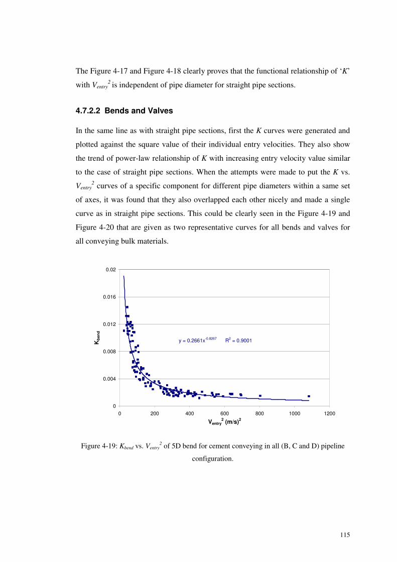
115
The Figure 4-17 and Figure 4-18 clearly proves that the functional relationship of ‘K’
with Ventry2 is independent of pipe diameter for straight pipe sections.
4.7.2.2 Bends and Valves
In the same line as with straight pipe sections, first the K curves were generated and
plotted against the square value of their individual entry velocities. They also show
the trend of power-law relationship of K with increasing entry velocity value similar
to the case of straight pipe sections. When the attempts were made to put the K vs.
Ventry2 curves of a specific component for different pipe diameters within a same set
of axes, it was found that they also overlapped each other nicely and made a single
curve as in straight pipe sections. This could be clearly seen in the Figure 4-19 and
Figure 4-20 that are given as two representative curves for all bends and valves for
all conveying bulk materials.
y = 0.2661x-0.8267 R2 = 0.9001
0
0.004
0.008
0.012
0.016
0.02
0 200 400 600 800 1000 1200
Ventry2 (m/s)2
Kb
end
Figure 4-19: Kbend vs. Ventry2 of 5D bend for cement conveying in all (B, C and D) pipeline
configuration.
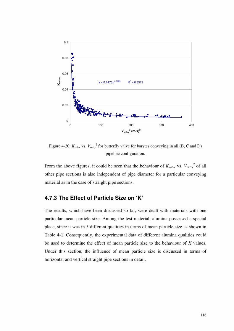
116
y = 0.1476x-0.6083 R2 = 0.8572
0
0.02
0.04
0.06
0.08
0.1
0 100 200 300 400
Ventry2 (m/s)2
Kva
lve
Figure 4-20: Kvalve vs. Ventry2 for butterfly valve for barytes conveying in all (B, C and D)
pipeline configuration.
From the above figures, it could be seen that the behaviour of Kvalve vs. Ventry2 of all
other pipe sections is also independent of pipe diameter for a particular conveying
material as in the case of straight pipe sections.
4.7.3 The Effect of Particle Size on ‘K’
The results, which have been discussed so far, were dealt with materials with one
particular mean particle size. Among the test material, alumina possessed a special
place, since it was in 5 different qualities in terms of mean particle size as shown in
Table 4-1. Consequently, the experimental data of different alumina qualities could
be used to determine the effect of mean particle size to the behaviour of K values.
Under this section, the influence of mean particle size is discussed in terms of
horizontal and vertical straight pipe sections in detail.
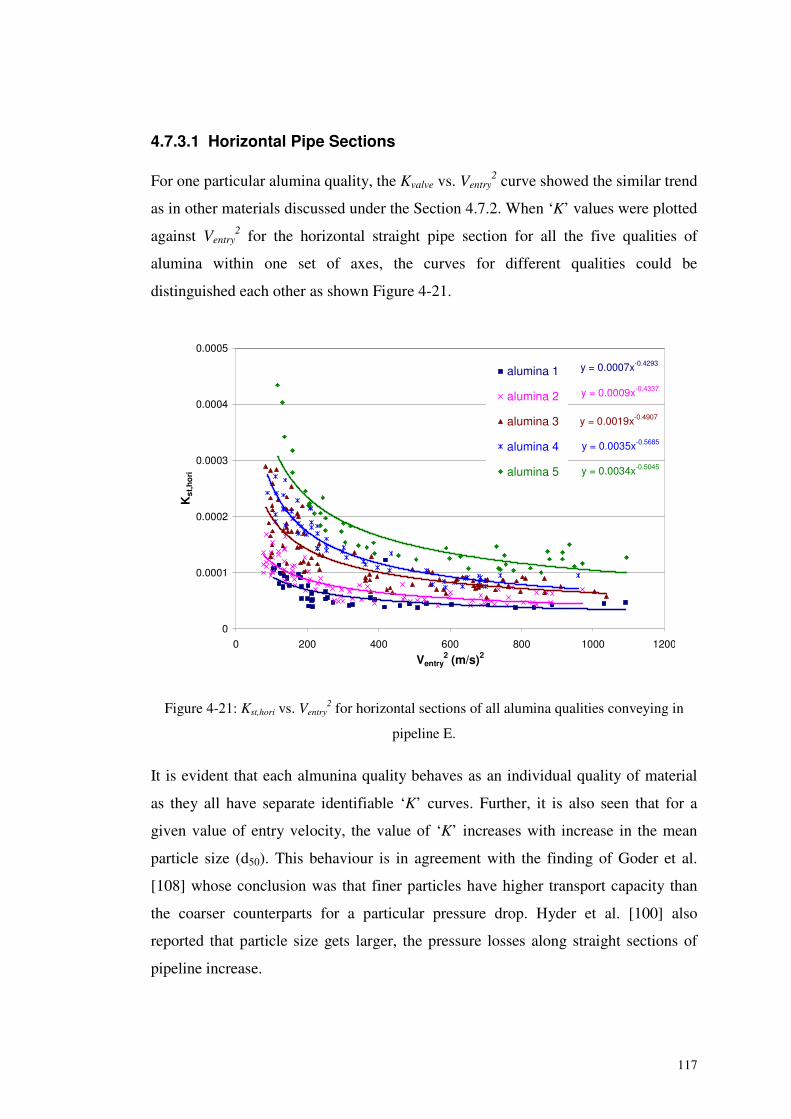
117
4.7.3.1 Horizontal Pipe Sections
For one particular alumina quality, the Kvalve vs. Ventry2 curve showed the similar trend
as in other materials discussed under the Section 4.7.2. When ‘K’ values were plotted
against Ventry2 for the horizontal straight pipe section for all the five qualities of
alumina within one set of axes, the curves for different qualities could be
distinguished each other as shown Figure 4-21.
y = 0.0034x-0.5045
y = 0.0035x-0.5685
y = 0.0007x-0.4293
y = 0.0019x-0.4907
y = 0.0009x-0.4337
0
0.0001
0.0002
0.0003
0.0004
0.0005
0 200 400 600 800 1000 1200
Ventry2 (m/s)2
Kst
,ho
ri
alumina 1
alumina 2
alumina 3
alumina 4
alumina 5
Figure 4-21: Kst,hori vs. Ventry2 for horizontal sections of all alumina qualities conveying in
pipeline E.
It is evident that each almunina quality behaves as an individual quality of material
as they all have separate identifiable ‘K’ curves. Further, it is also seen that for a
given value of entry velocity, the value of ‘K’ increases with increase in the mean
particle size (d50). This behaviour is in agreement with the finding of Goder et al.
[108] whose conclusion was that finer particles have higher transport capacity than
the coarser counterparts for a particular pressure drop. Hyder et al. [100] also
reported that particle size gets larger, the pressure losses along straight sections of
pipeline increase.
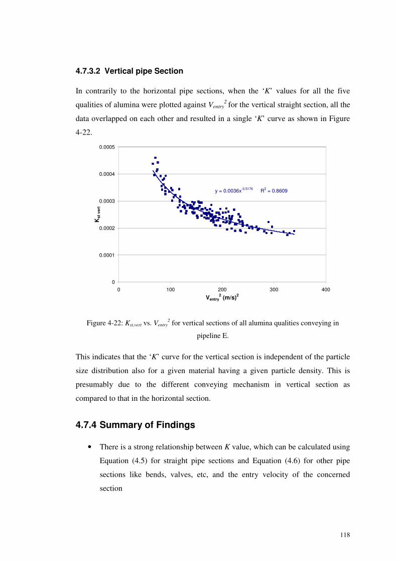
118
4.7.3.2 Vertical pipe Section
In contrarily to the horizontal pipe sections, when the ‘K’ values for all the five
qualities of alumina were plotted against Ventry2 for the vertical straight section, all the
data overlapped on each other and resulted in a single ‘K’ curve as shown in Figure
4-22.
y = 0.0036x-0.5176 R2 = 0.8609
0
0.0001
0.0002
0.0003
0.0004
0.0005
0 100 200 300 400
Ventry2 (m/s)2
Kst
vert
Figure 4-22: Kst,vert vs. Ventry2 for vertical sections of all alumina qualities conveying in
pipeline E.
This indicates that the ‘K’ curve for the vertical section is independent of the particle
size distribution also for a given material having a given particle density. This is
presumably due to the different conveying mechanism in vertical section as
compared to that in the horizontal section.
4.7.4 Summary of Findings
• There is a strong relationship between K value, which can be calculated using
Equation (4.5) for straight pipe sections and Equation (4.6) for other pipe
sections like bends, valves, etc, and the entry velocity of the concerned
section
119
• The behaviour of ‘K’ vs. Ventry2 curves for straight section and other pipe
components shows a common trend of power-law relationship with
increasing entry velocity for all conveying bulk materials tested. The K factor
could be explained as a parameter, which is very sensitive to the entry section
velocity in dense phase conveying. In dilute phase region, the gas-solid flow
becomes an approximation to a single phase flow with less influence from
solid particles, thus the K behaves like the friction factor for conveying gas.
• The relationship between K and Ventry2 is independent of pipe diameter for all
pipe sections.
• The behaviour of ‘K’ vs. Ventry2 for horizontal pipe sections is dependent on
the mean particle size of the conveying material, while the same for vertical
pipe sections is independent of particle size. This finding facilitates to avoid
the elaborate tests for different qualities (in terms of mean particle size) of a
given material with vertical sections.
4.8 Model Validation
Having thus established the functional relationship of K and Ventry, the next stage was
to validate the model with the help of available experimental data. For this purpose,
the K vs. Ventry2 curves generated by combining the results of all pipe sizes were used
to define the relationship between K value and the entry velocity of the concerned
component. Then, these relationships were used to calculate the pressure drop values
across individual features. Finally the calculated pressure values were compared with
the experimental values. Under this section, calculation procedure, results and
comparison of validation are discussed in detail.
4.8.1 Calculation Procedure of Validation
In the calculation procedure, the whole pipeline was considered as a virtual
combination of short horizontal and vertical pipe sections, individual bends and other
pipe components like valves. As discussed under the theoretical consideration, the
concept of suspension density is best suited for rather short pipe sections. Hence any
120
straight horizontal or vertical pipe section was considered to be made up of virtual
small sections each of 1m length.
The calculation procedure began with the available experimental conditions at the
starting point of conveying loop. At the starting point, the pressure available just
outside the blow tank was taken as the reference point and calculation proceeded
along the pipeline by calculating the pressure drop of each individual section of the
conveying loop. The exit pressure condition of the concerned section is updated by
adding the calculated pressure drop to the start pressure value. The pressure available
at the exit of one section was used as the entry condition to the next section.
However, the bends, valves etc were considered as individual units and pressure
losses incurred with them were calculated individually. This procedure can briefly be
represented as shown in Figure 4-23. This calculation procedure was continued by
updating the pressure value of the entry section of the consecutive section, from
starting point of the conveying line until the receiving tank.
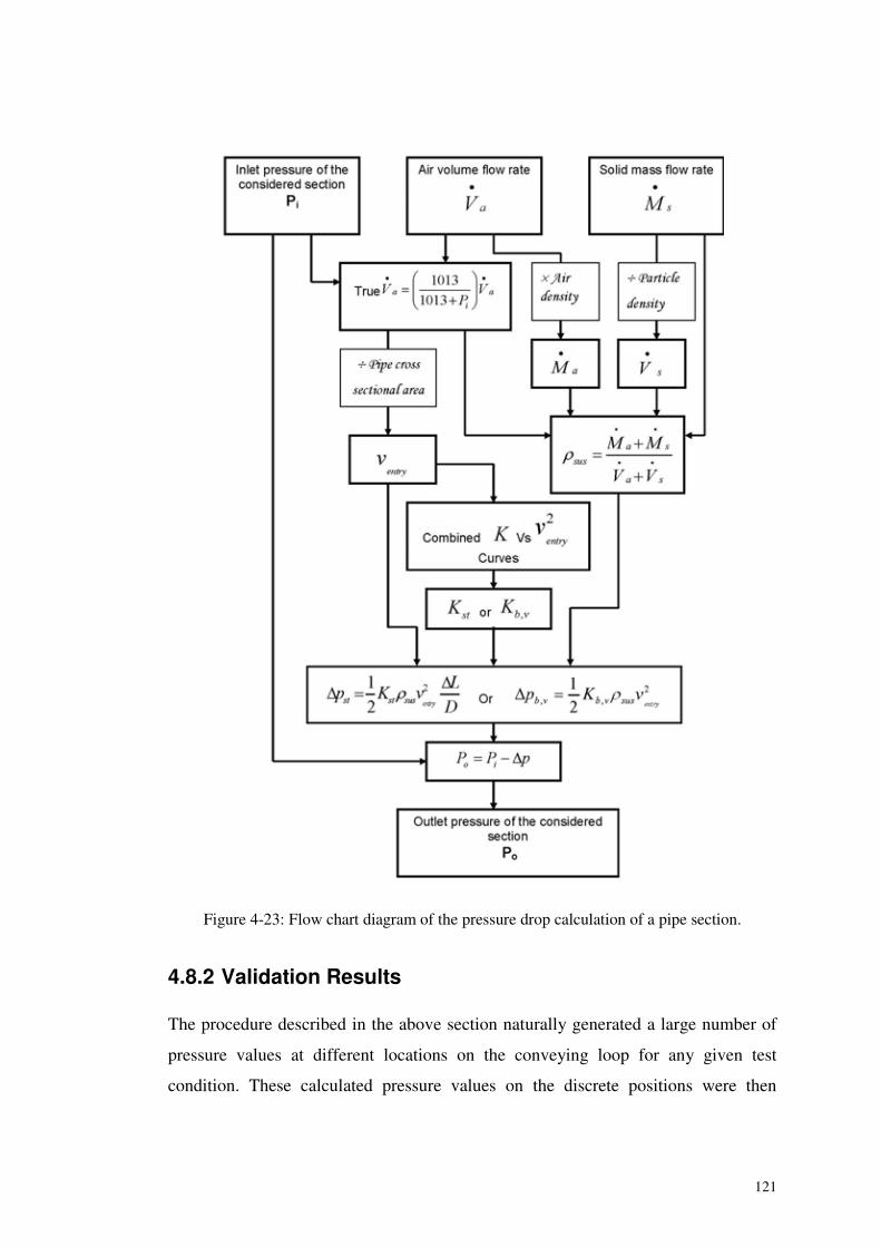
121
Figure 4-23: Flow chart diagram of the pressure drop calculation of a pipe section.
4.8.2 Validation Results
The procedure described in the above section naturally generated a large number of
pressure values at different locations on the conveying loop for any given test
condition. These calculated pressure values on the discrete positions were then
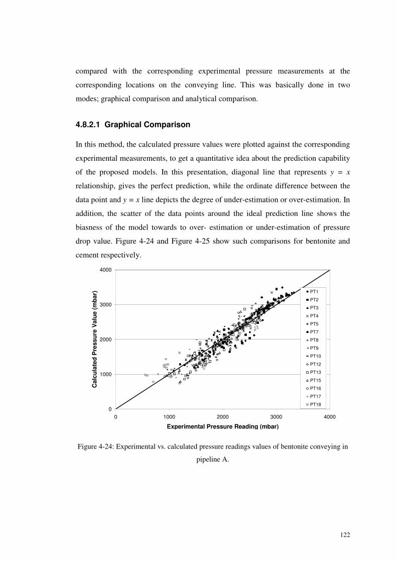
122
compared with the corresponding experimental pressure measurements at the
corresponding locations on the conveying line. This was basically done in two
modes; graphical comparison and analytical comparison.
4.8.2.1 Graphical Comparison
In this method, the calculated pressure values were plotted against the corresponding
experimental measurements, to get a quantitative idea about the prediction capability
of the proposed models. In this presentation, diagonal line that represents y = x
relationship, gives the perfect prediction, while the ordinate difference between the
data point and y = x line depicts the degree of under-estimation or over-estimation. In
addition, the scatter of the data points around the ideal prediction line shows the
biasness of the model towards to over- estimation or under-estimation of pressure
drop value. Figure 4-24 and Figure 4-25 show such comparisons for bentonite and
cement respectively.
0
1000
2000
3000
4000
0 1000 2000 3000 4000
Experimental Pressure Reading (mbar)
Cal
cula
ted
Pre
ssu
reV
alu
e(m
bar
) PT1
PT2
PT3
PT4
PT5
PT7
PT8
PT9
PT10
PT12
PT13
PT15
PT16
PT17
PT18
Figure 4-24: Experimental vs. calculated pressure readings values of bentonite conveying in
pipeline A.
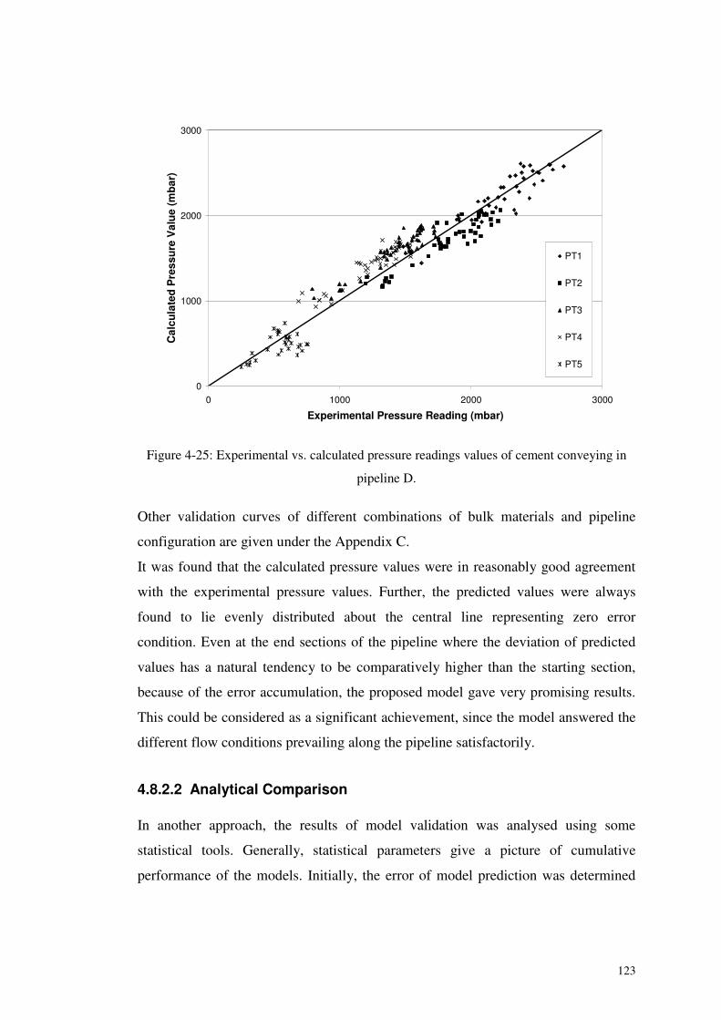
123
0
1000
2000
3000
0 1000 2000 3000
Experimental Pressure Reading (mbar)
Cal
cula
ted
Pre
ssu
reV
alu
e(m
bar
)
PT1
PT2
PT3
PT4
PT5
Figure 4-25: Experimental vs. calculated pressure readings values of cement conveying in
pipeline D.
Other validation curves of different combinations of bulk materials and pipeline
configuration are given under the Appendix C.
It was found that the calculated pressure values were in reasonably good agreement
with the experimental pressure values. Further, the predicted values were always
found to lie evenly distributed about the central line representing zero error
condition. Even at the end sections of the pipeline where the deviation of predicted
values has a natural tendency to be comparatively higher than the starting section,
because of the error accumulation, the proposed model gave very promising results.
This could be considered as a significant achievement, since the model answered the
different flow conditions prevailing along the pipeline satisfactorily.
4.8.2.2 Analytical Comparison
In another approach, the results of model validation was analysed using some
statistical tools. Generally, statistical parameters give a picture of cumulative
performance of the models. Initially, the error of model prediction was determined
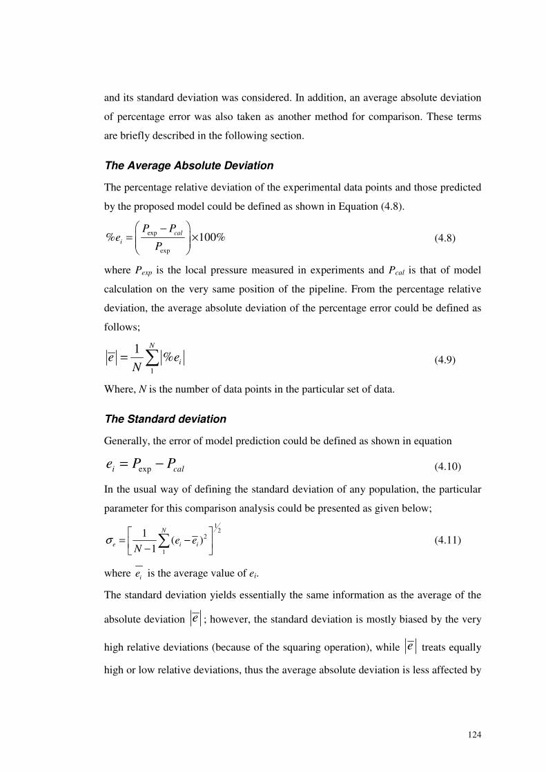
124
and its standard deviation was considered. In addition, an average absolute deviation
of percentage error was also taken as another method for comparison. These terms
are briefly described in the following section.
The Average Absolute Deviation
The percentage relative deviation of the experimental data points and those predicted
by the proposed model could be defined as shown in Equation (4.8).
exp
exp
% 100%cali
P Pe
P
−= ×� �� ��
(4.8)
where Pexp is the local pressure measured in experiments and Pcal is that of model
calculation on the very same position of the pipeline. From the percentage relative
deviation, the average absolute deviation of the percentage error could be defined as
follows;
1
1%
N
ie eN
= � (4.9)
Where, N is the number of data points in the particular set of data.
The Standard deviation
Generally, the error of model prediction could be defined as shown in equation
expi cale P P= − (4.10)
In the usual way of defining the standard deviation of any population, the particular
parameter for this comparison analysis could be presented as given below;
12
2
1
1( )
1
N
e i ie eN
σ � �= −� �−� �� (4.11)
where ie is the average value of ei.
The standard deviation yields essentially the same information as the average of the
absolute deviation e ; however, the standard deviation is mostly biased by the very
high relative deviations (because of the squaring operation), while e treats equally
high or low relative deviations, thus the average absolute deviation is less affected by
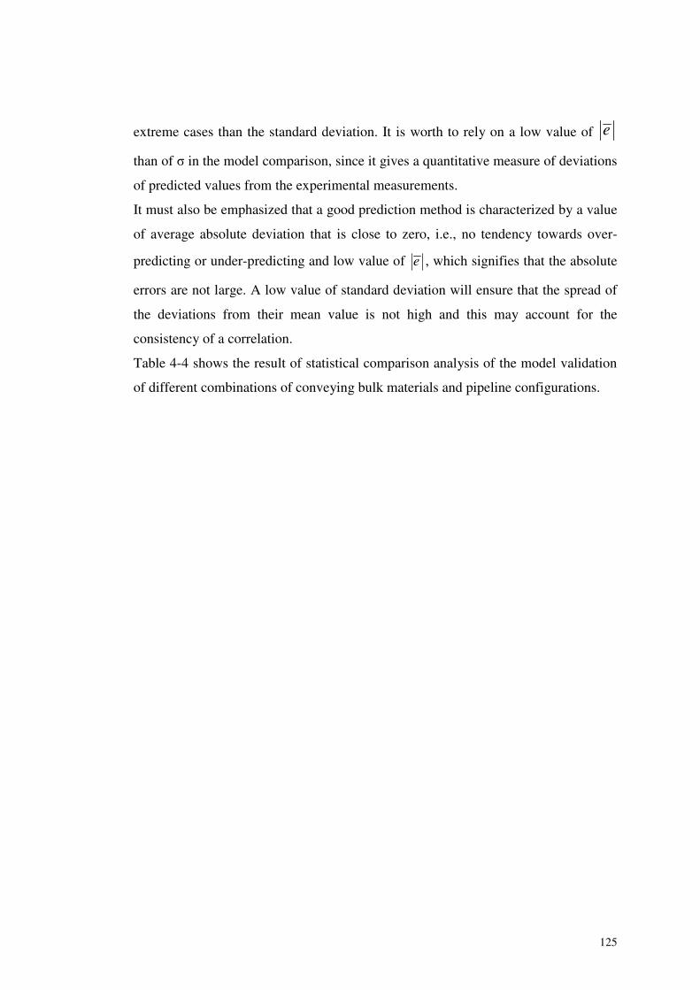
125
extreme cases than the standard deviation. It is worth to rely on a low value of e
than of � in the model comparison, since it gives a quantitative measure of deviations
of predicted values from the experimental measurements.
It must also be emphasized that a good prediction method is characterized by a value
of average absolute deviation that is close to zero, i.e., no tendency towards over-
predicting or under-predicting and low value of e , which signifies that the absolute
errors are not large. A low value of standard deviation will ensure that the spread of
the deviations from their mean value is not high and this may account for the
consistency of a correlation.
Table 4-4 shows the result of statistical comparison analysis of the model validation
of different combinations of conveying bulk materials and pipeline configurations.
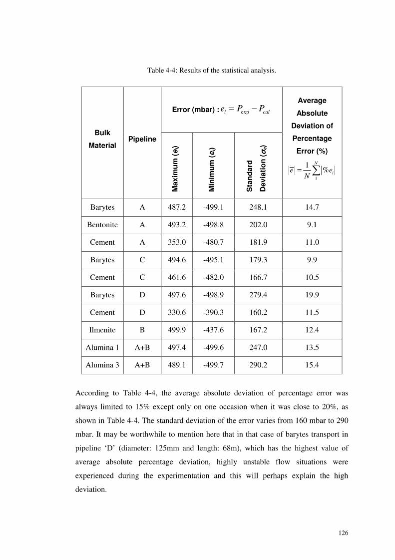
126
Table 4-4: Results of the statistical analysis.
According to Table 4-4, the average absolute deviation of percentage error was
always limited to 15% except only on one occasion when it was close to 20%, as
shown in Table 4-4. The standard deviation of the error varies from 160 mbar to 290
mbar. It may be worthwhile to mention here that in that case of barytes transport in
pipeline ‘D’ (diameter: 125mm and length: 68m), which has the highest value of
average absolute percentage deviation, highly unstable flow situations were
experienced during the experimentation and this will perhaps explain the high
deviation.
Error (mbar) : expi cale P P= −
Bulk
MaterialPipeline
Max
imu
m(e
i)
Min
imu
m(e
i)
Sta
nd
ard
Dev
iati
on
( σσ σσe)
Average
Absolute
Deviation of
Percentage
Error (%)
1
1%
N
ie eN
= �
Barytes A 487.2 -499.1 248.1 14.7
Bentonite A 493.2 -498.8 202.0 9.1
Cement A 353.0 -480.7 181.9 11.0
Barytes C 494.6 -495.1 179.3 9.9
Cement C 461.6 -482.0 166.7 10.5
Barytes D 497.6 -498.9 279.4 19.9
Cement D 330.6 -390.3 160.2 11.5
Ilmenite B 499.9 -437.6 167.2 12.4
Alumina 1 A+B 497.4 -499.6 247.0 13.5
Alumina 3 A+B 489.1 -499.7 290.2 15.4
127
4.9 Summary
The proposed model based on the piece-wise approach of scaling and well-known
Darcy-Weisbach’s equation was described with all conditions and applications. The
series of tests carried out to establish and validate the proposed model were
explained in detail including the information of test materials and test setup. Finally,
the model validation procedure and comparison results were presented also in
graphical and analytical forms.
128
5 COMPARISON ANALYSIS OF ‘K’ FACTORMETHOD WITH OTHER MODELS
5.1 Introduction
As explained in Chapters 4, the proposed scaling up model has shown good
agreement with experimental measurements when it was tested with different bulk
materials and pipeline configurations. In addition to validation of the model with the
experimental observations, a comparison with other models was also done with the
help of available test data. The objective of this work was to compare the
performance of the proposed model with some other well-known scaling and
pressure drop determination models with different materials and pipeline
configurations.
Among the published scaling up techniques and pressure drop determination models,
four methods have been selected for this investigation, as they are often referred in
the literature. The chosen techniques are rather straightforward, as compared with the
other techniques reported in the literature and are claimed to have better agreements
with the experimental observations.
In order to examine the effect of pipeline diameter, length and the number of bends
in the scaling method, different pipeline configurations have been selected. In the
first stage, the models were tested with isolated straight pipe sections and the whole
conveying circuit was addressed in the second stage of comparison. The
experimental observations on a particular pipeline were used to predict the pressure
drop values of other pipeline configuration, using different scaling models and then
the calculated pressure drop values have been compared with the experimentally
obtained pressure drop values. Some statistical tools have been used for the
comparison. Calculation procedure, comparison methods, results and discussion are
given in detail in this Chapter.
129
5.2 Outline of Scaling Techniques
As discussed in Chapter 2, there are basically two distinguished concepts used in
empirical models of pressure drop determination of pneumatic conveying systems.
One group considers the gas-solid flow as a mixture and defines the relevant
parameters with respect to it. The other group splits the mixture into two different
hypothetical components as gas flow and solid flow and characterizes the parameters
like friction factor, etc, individually for them. As an alternative design method of
pneumatic conveying systems, scaling up techniques also use two different
approaches; namely global approach and piece wise approach.
Four different models, which represent all the different groups and approaches
explained above, were selected, for this comparative analysis, with the aim of
comparing the model proposed by author with all available methods of pressure drop
determination in pneumatic conveying systems. The methods used are;
1. Weber’s pressure drop determination method [43]
2. Pan’s scaling up technique [22]
3. Keys and Chambers scaling model [95]
4. Molerus scaling method [91]
These models were described in detail in Section 2.9. In Weber method [43], the gas-
solid flow is considered as a mixture and an empirical method is proposed to
determine the friction factor of the whole mixture. The friction factor is considered to
be a function of solids loading ratio and Froude number. The empirical coefficients
are proposed to be the same for a particulate bulk material and independent of
geometrical parameters of the pipeline. This method is claimed to be suitable for
dilute phase transport.
Following the common approach of pressure drop determination where the gas-solid
flow is considered as a combination of two distinguished hypothetical components of
gas and solid, Pan and Wypych proposed a scaling up technique [22]. According to
them, the pressure drop of the pneumatic transport of air-sold mixture is composed of
component due to air only and of an additional component due to the solid part,
which are independent from each other. They proposed [22, 46] two different
130
empirical models to determine the friction factors of each phases as a function of
solids loading, Froude number and mean density of air, using dimensional analysis.
Based on the experimental data of pressures across straight sections and bends,
exponents of the empirical relationship are determined by minimising the sum of
square errors of pressures. These exponents, as in the previous cases, are valid for the
given product and independent of pipe geometry.
Keys and Chambers [95] preferred the global approach and proposed a method based
on an empirical correlation. This method combines a number of non-dimensional
flow parameters to predict the pressure loss in the pipeline system. The effects of
conveying gas and bulk solid were considered separately, but, by addressing the
whole pipeline together with the bends. Empirical correlations were obtained for gas
and solid friction factors and used them to predict the pressure drop of another
system that conveys the same bulk material.
Molerus [91] considered a unique relationship between two non-dimensional
parameters; solid friction factor and Froude number of gas to define the gas-solid
flow of given combination of gas and particulate material. He proposed to carry out
pilot plant tests to get the data in terms of solid friction factor versus Froude number
of gas and to use the resulting curve for the prediction of the pressure drop of the
plant to be designed for conveying the same bulk material.
5.3 Method of Comparison
To evaluate the performances of different models, their predictions were compared
with corresponding experimental data. This was done using both graphical method
and statistical method. A brief description of these two methods was given in Section
4.8.2.
5.4 Test Setup and Conveying Materials
The test data generated by the main investigation were utilised for the comparative
analysis. For the convenience of identification of pipe configurations and positions of
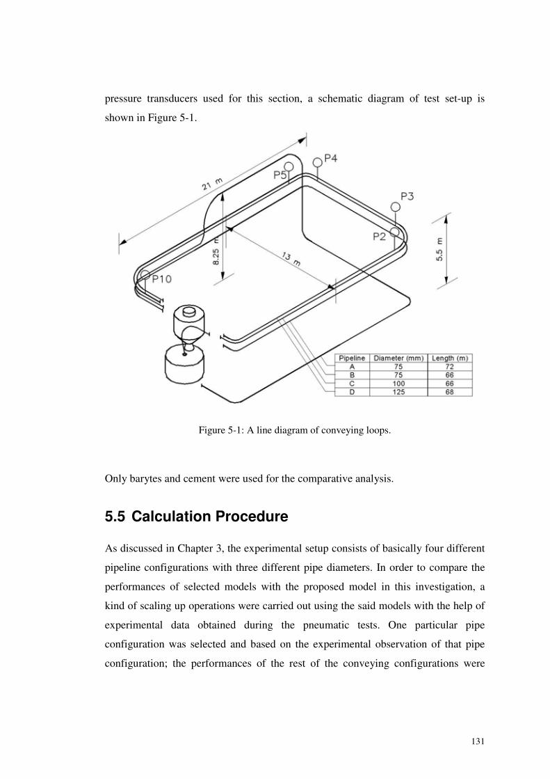
131
pressure transducers used for this section, a schematic diagram of test set-up is
shown in Figure 5-1.
Figure 5-1: A line diagram of conveying loops.
Only barytes and cement were used for the comparative analysis.
5.5 Calculation Procedure
As discussed in Chapter 3, the experimental setup consists of basically four different
pipeline configurations with three different pipe diameters. In order to compare the
performances of selected models with the proposed model in this investigation, a
kind of scaling up operations were carried out using the said models with the help of
experimental data obtained during the pneumatic tests. One particular pipe
configuration was selected and based on the experimental observation of that pipe
configuration; the performances of the rest of the conveying configurations were
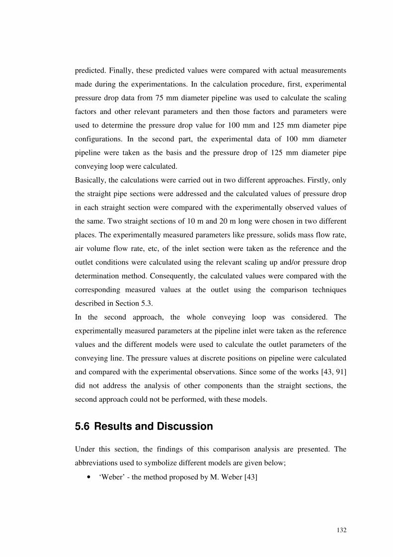
132
predicted. Finally, these predicted values were compared with actual measurements
made during the experimentations. In the calculation procedure, first, experimental
pressure drop data from 75 mm diameter pipeline was used to calculate the scaling
factors and other relevant parameters and then those factors and parameters were
used to determine the pressure drop value for 100 mm and 125 mm diameter pipe
configurations. In the second part, the experimental data of 100 mm diameter
pipeline were taken as the basis and the pressure drop of 125 mm diameter pipe
conveying loop were calculated.
Basically, the calculations were carried out in two different approaches. Firstly, only
the straight pipe sections were addressed and the calculated values of pressure drop
in each straight section were compared with the experimentally observed values of
the same. Two straight sections of 10 m and 20 m long were chosen in two different
places. The experimentally measured parameters like pressure, solids mass flow rate,
air volume flow rate, etc, of the inlet section were taken as the reference and the
outlet conditions were calculated using the relevant scaling up and/or pressure drop
determination method. Consequently, the calculated values were compared with the
corresponding measured values at the outlet using the comparison techniques
described in Section 5.3.
In the second approach, the whole conveying loop was considered. The
experimentally measured parameters at the pipeline inlet were taken as the reference
values and the different models were used to calculate the outlet parameters of the
conveying line. The pressure values at discrete positions on pipeline were calculated
and compared with the experimental observations. Since some of the works [43, 91]
did not address the analysis of other components than the straight sections, the
second approach could not be performed, with these models.
5.6 Results and Discussion
Under this section, the findings of this comparison analysis are presented. The
abbreviations used to symbolize different models are given below;
• ‘Weber’ - the method proposed by M. Weber [43]
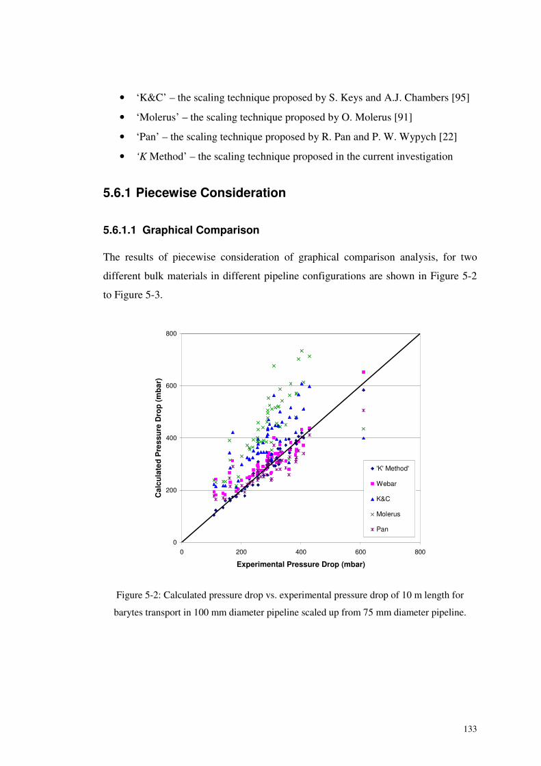
133
• ‘K&C’ – the scaling technique proposed by S. Keys and A.J. Chambers [95]
• ‘Molerus’ – the scaling technique proposed by O. Molerus [91]
• ‘Pan’ – the scaling technique proposed by R. Pan and P. W. Wypych [22]
• ‘K Method’ – the scaling technique proposed in the current investigation
5.6.1 Piecewise Consideration
5.6.1.1 Graphical Comparison
The results of piecewise consideration of graphical comparison analysis, for two
different bulk materials in different pipeline configurations are shown in Figure 5-2
to Figure 5-3.
0
200
400
600
800
0 200 400 600 800
Experimental Pressure Drop (mbar)
Cal
cula
ted
Pre
ssu
reD
rop
(mb
ar)
'K' Method'
Webar
K&C
Molerus
Pan
Figure 5-2: Calculated pressure drop vs. experimental pressure drop of 10 m length for
barytes transport in 100 mm diameter pipeline scaled up from 75 mm diameter pipeline.
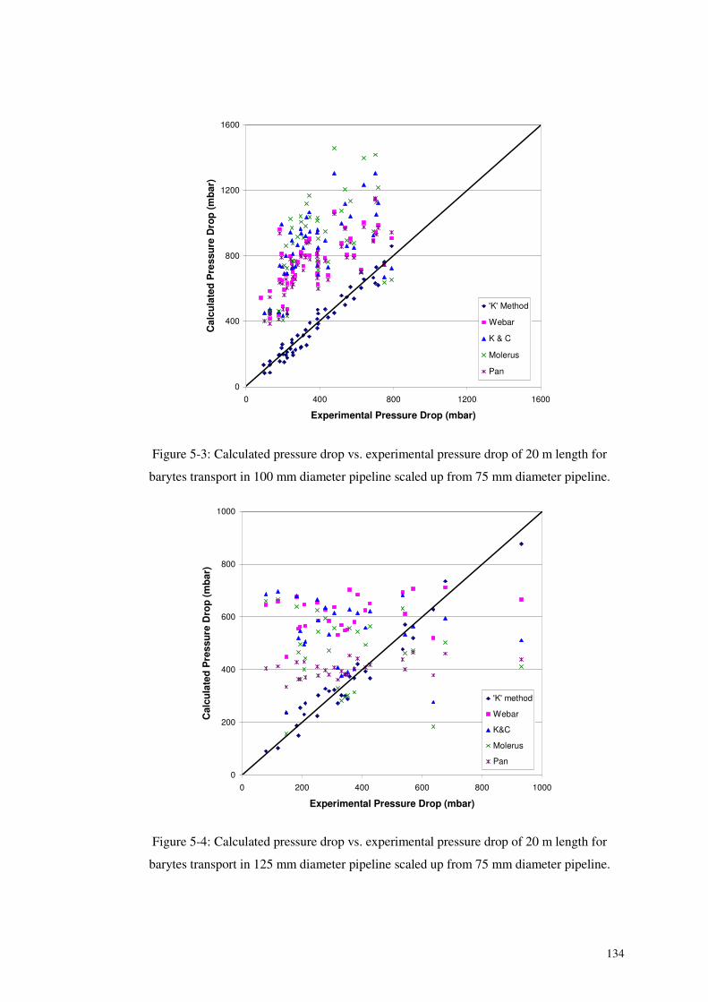
134
0
400
800
1200
1600
0 400 800 1200 1600
Experimental Pressure Drop (mbar)
Cal
cula
ted
Pre
ssur
eD
rop
(mb
ar)
'K' Method
Webar
K & C
Molerus
Pan
Figure 5-3: Calculated pressure drop vs. experimental pressure drop of 20 m length for
barytes transport in 100 mm diameter pipeline scaled up from 75 mm diameter pipeline.
0
200
400
600
800
1000
0 200 400 600 800 1000
Experimental Pressure Drop (mbar)
Cal
cula
ted
Pre
ssur
eD
rop
(mb
ar)
'K' method
Webar
K&C
Molerus
Pan
Figure 5-4: Calculated pressure drop vs. experimental pressure drop of 20 m length for
barytes transport in 125 mm diameter pipeline scaled up from 75 mm diameter pipeline.
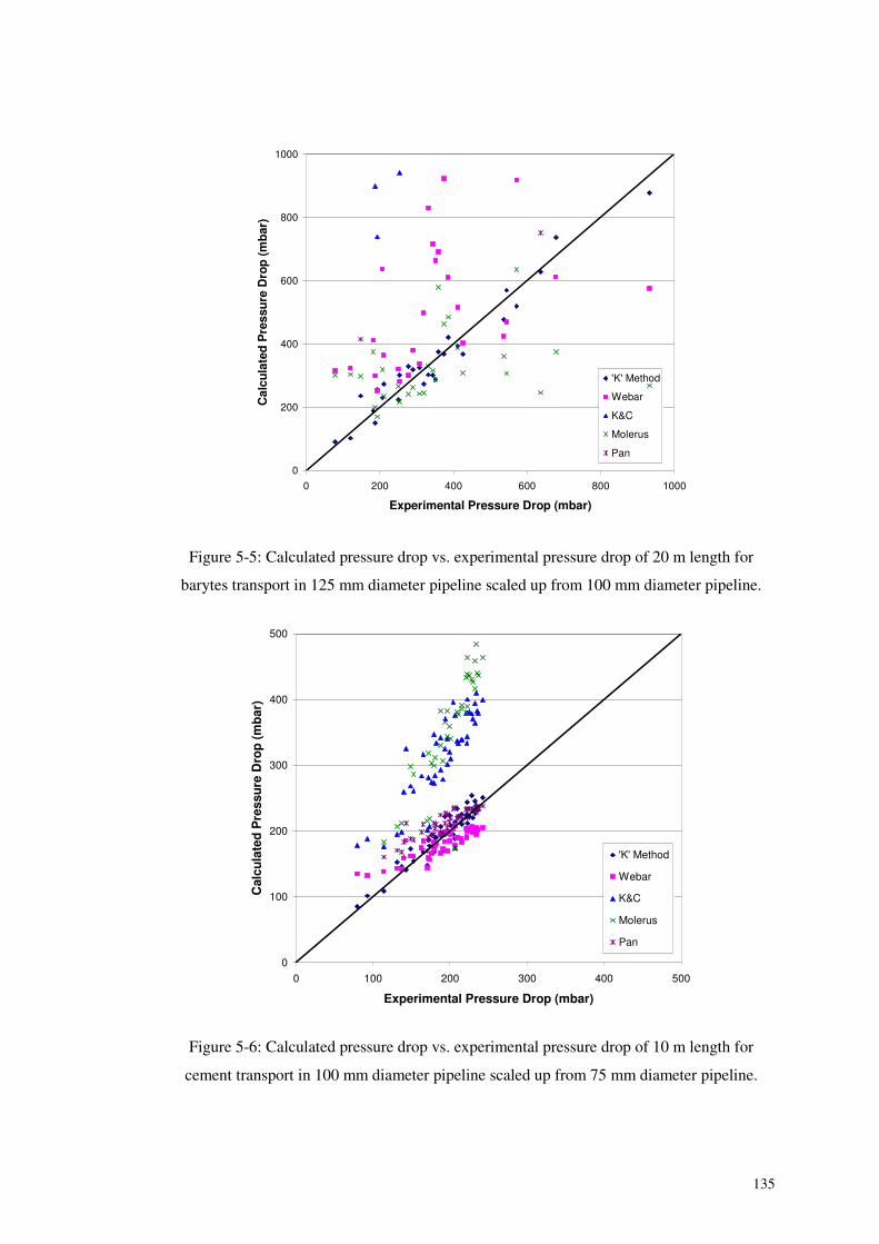
135
0
200
400
600
800
1000
0 200 400 600 800 1000
Experimental Pressure Drop (mbar)
Cal
cula
ted
Pre
ssu
reD
rop
(mb
ar)
'K' Method
Webar
K&C
Molerus
Pan
Figure 5-5: Calculated pressure drop vs. experimental pressure drop of 20 m length for
barytes transport in 125 mm diameter pipeline scaled up from 100 mm diameter pipeline.
0
100
200
300
400
500
0 100 200 300 400 500
Experimental Pressure Drop (mbar)
Cal
cula
ted
Pre
ssu
reD
rop
(mb
ar)
'K' Method
Webar
K&C
Molerus
Pan
Figure 5-6: Calculated pressure drop vs. experimental pressure drop of 10 m length for
cement transport in 100 mm diameter pipeline scaled up from 75 mm diameter pipeline.
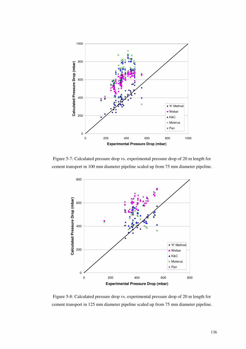
136
0
200
400
600
800
1000
0 200 400 600 800 1000
Experimental Pressure Drop (mbar)
Cal
cula
ted
Pre
ssu
reD
rop
(mb
ar)
'K' Method
Webar
K&C
Molerus
Pan
Figure 5-7: Calculated pressure drop vs. experimental pressure drop of 20 m length for
cement transport in 100 mm diameter pipeline scaled up from 75 mm diameter pipeline.
0
200
400
600
800
0 200 400 600 800
Experimental Pressure Drop (mbar)
Cal
cula
ted
Pre
ssu
reD
rop
(mb
ar)
'K' Method
Webar
K&C
Molerus
Pan
Figure 5-8: Calculated pressure drop vs. experimental pressure drop of 20 m length for
cement transport in 125 mm diameter pipeline scaled up from 75 mm diameter pipeline.
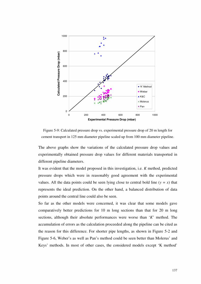
137
0
200
400
600
800
1000
0 200 400 600 800 1000
Experimental Pressure Drop (mbar)
Cal
cula
ted
Pre
ssu
reD
rop
(mb
ar)
'K' Method
Webar
K&C
Molerus
Pan
Figure 5-9: Calculated pressure drop vs. experimental pressure drop of 20 m length for
cement transport in 125 mm diameter pipeline scaled up from 100 mm diameter pipeline.
The above graphs show the variations of the calculated pressure drop values and
experimentally obtained pressure drop values for different materials transported in
different pipeline diameters.
It was evident that the model proposed in this investigation, i.e. K method, predicted
pressure drops which were in reasonably good agreement with the experimental
values. All the data points could be seen lying close to central bold line (y = x) that
represents the ideal prediction. On the other hand, a balanced distribution of data
points around the central line could also be seen.
So far as the other models were concerned, it was clear that some models gave
comparatively better predictions for 10 m long sections than that for 20 m long
sections, although their absolute performances were worse than ‘K’ method. The
accumulation of errors as the calculation proceeded along the pipeline can be cited as
the reason for this difference. For shorter pipe lengths, as shown in Figure 5-2 and
Figure 5-6, Weber’s as well as Pan’s method could be seen better than Molerus’ and
Keys’ methods. In most of other cases, the considered models except ‘K method’
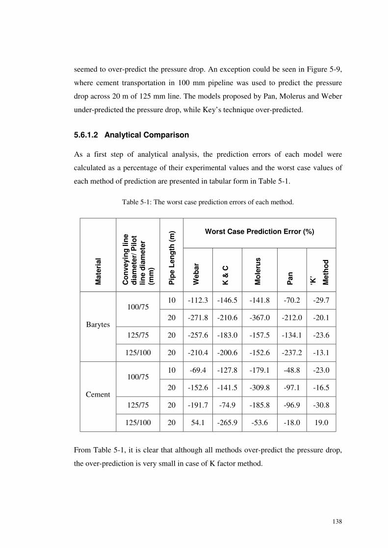
138
seemed to over-predict the pressure drop. An exception could be seen in Figure 5-9,
where cement transportation in 100 mm pipeline was used to predict the pressure
drop across 20 m of 125 mm line. The models proposed by Pan, Molerus and Weber
under-predicted the pressure drop, while Key’s technique over-predicted.
5.6.1.2 Analytical Comparison
As a first step of analytical analysis, the prediction errors of each model were
calculated as a percentage of their experimental values and the worst case values of
each method of prediction are presented in tabular form in Table 5-1.
Table 5-1: The worst case prediction errors of each method.
From Table 5-1, it is clear that although all methods over-predict the pressure drop,
the over-prediction is very small in case of K factor method.
Worst Case Prediction Error (%)
Mat
eria
l
Co
nve
yin
glin
ed
iam
eter
/Pilo
tlin
ed
iam
eter
(mm
)
Pip
eL
eng
th(m
)
Web
ar
K&
C
Mo
leru
s
Pan
‘K’
Met
ho
d
10 -112.3 -146.5 -141.8 -70.2 -29.7100/75
20 -271.8 -210.6 -367.0 -212.0 -20.1
125/75 20 -257.6 -183.0 -157.5 -134.1 -23.6Barytes
125/100 20 -210.4 -200.6 -152.6 -237.2 -13.1
10 -69.4 -127.8 -179.1 -48.8 -23.0100/75
20 -152.6 -141.5 -309.8 -97.1 -16.5
125/75 20 -191.7 -74.9 -185.8 -96.9 -30.8Cement
125/100 20 54.1 -265.9 -53.6 -18.0 19.0
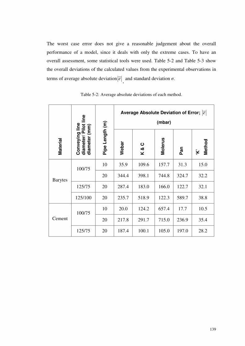
139
The worst case error does not give a reasonable judgement about the overall
performance of a model, since it deals with only the extreme cases. To have an
overall assessment, some statistical tools were used. Table 5-2 and Table 5-3 show
the overall deviations of the calculated values from the experimental observations in
terms of average absolute deviation e,
and standard deviation �.
Table 5-2: Average absolute deviations of each method.
Average Absolute Deviation of Error; e
(mbar)
Mat
eria
l
Co
nve
yin
glin
ed
iam
eter
/Pilo
tlin
ed
iam
eter
(mm
)
Pip
eL
eng
th(m
)
Web
ar
K&
C
Mo
leru
s
Pan
‘K’
Met
ho
d
10 35.9 109.6 157.7 31.3 15.0100/75
20 344.4 398.1 744.8 324.7 32.2
125/75 20 287.4 183.0 166.0 122.7 32.1Barytes
125/100 20 235.7 518.9 122.3 589.7 38.8
10 20.0 124.2 657.4 17.7 10.5100/75
20 217.8 291.7 715.0 236.9 35.4Cement
125/75 20 187.4 100.1 105.0 197.0 28.2
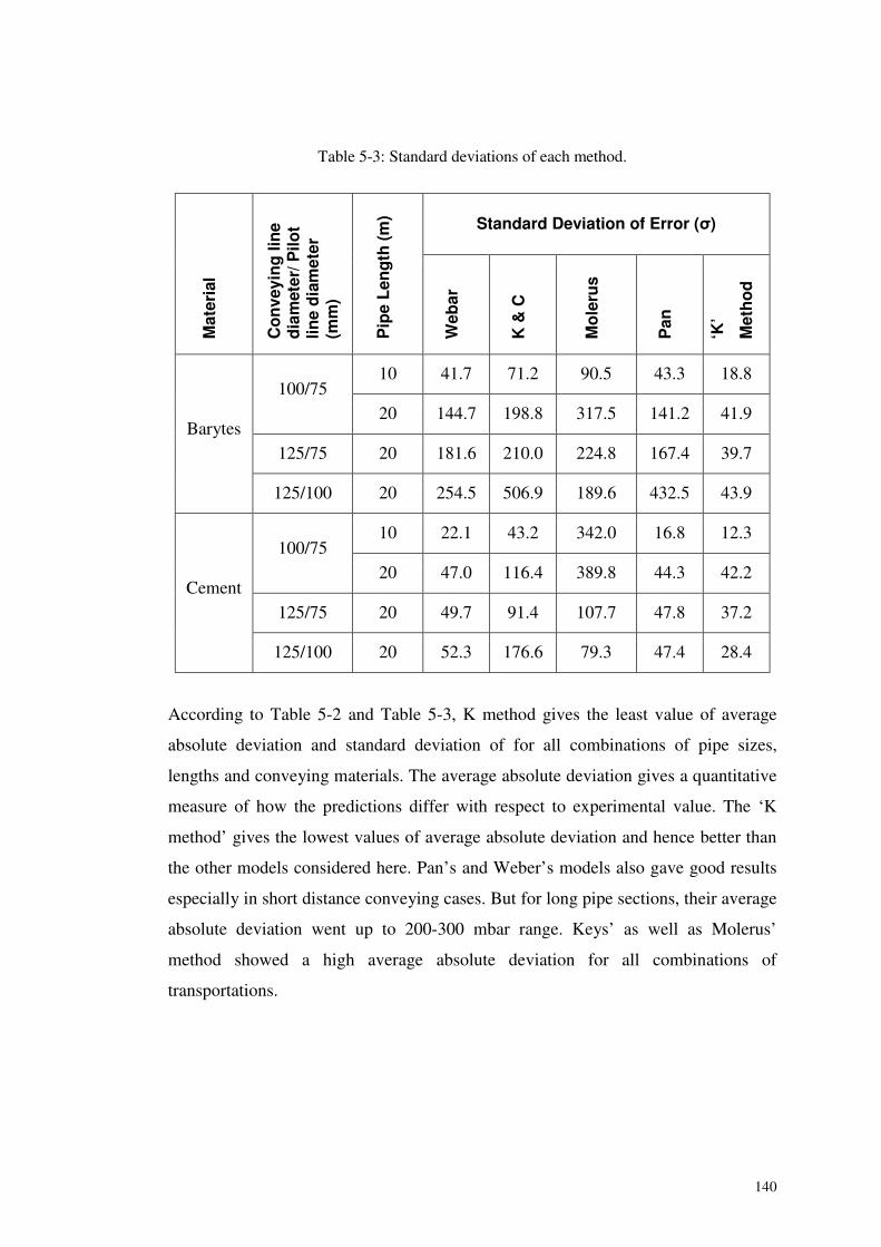
140
Table 5-3: Standard deviations of each method.
According to Table 5-2 and Table 5-3, K method gives the least value of average
absolute deviation and standard deviation of for all combinations of pipe sizes,
lengths and conveying materials. The average absolute deviation gives a quantitative
measure of how the predictions differ with respect to experimental value. The ‘K
method’ gives the lowest values of average absolute deviation and hence better than
the other models considered here. Pan’s and Weber’s models also gave good results
especially in short distance conveying cases. But for long pipe sections, their average
absolute deviation went up to 200-300 mbar range. Keys’ as well as Molerus’
method showed a high average absolute deviation for all combinations of
transportations.
Standard Deviation of Error (�)M
ater
ial
Co
nve
yin
glin
ed
iam
eter
/Pilo
tlin
ed
iam
eter
(mm
)
Pip
eL
eng
th(m
)
Web
ar
K&
C
Mo
leru
s
Pan
‘K’
Met
ho
d
10 41.7 71.2 90.5 43.3 18.8100/75
20 144.7 198.8 317.5 141.2 41.9
125/75 20 181.6 210.0 224.8 167.4 39.7Barytes
125/100 20 254.5 506.9 189.6 432.5 43.9
10 22.1 43.2 342.0 16.8 12.3100/75
20 47.0 116.4 389.8 44.3 42.2
125/75 20 49.7 91.4 107.7 47.8 37.2Cement
125/100 20 52.3 176.6 79.3 47.4 28.4
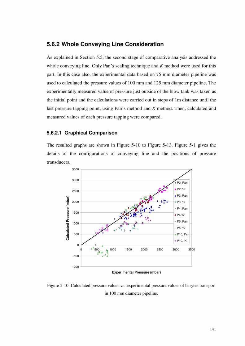
141
5.6.2 Whole Conveying Line Consideration
As explained in Section 5.5, the second stage of comparative analysis addressed the
whole conveying line. Only Pan’s scaling technique and K method were used for this
part. In this case also, the experimental data based on 75 mm diameter pipeline was
used to calculated the pressure values of 100 mm and 125 mm diameter pipeline. The
experimentally measured value of pressure just outside of the blow tank was taken as
the initial point and the calculations were carried out in steps of 1m distance until the
last pressure tapping point, using Pan’s method and K method. Then, calculated and
measured values of each pressure tapping were compared.
5.6.2.1 Graphical Comparison
The resulted graphs are shown in Figure 5-10 to Figure 5-13. Figure 5-1 gives the
details of the configurations of conveying line and the positions of pressure
transducers.
-1000
-500
0
500
1000
1500
2000
2500
3000
3500
0 500 1000 1500 2000 2500 3000 3500
Experimental Pressure (mbar)
Cal
cula
ted
Pre
ssu
re(m
bar
)
P2, Pan
P2, 'K'
P3, Pan
P3, 'K'
P4, Pan
P4,'K'
P5, Pan
P5, 'K'
P10, Pan
P10, 'K'
Figure 5-10: Calculated pressure values vs. experimental pressure values of barytes transport
in 100 mm diameter pipeline.
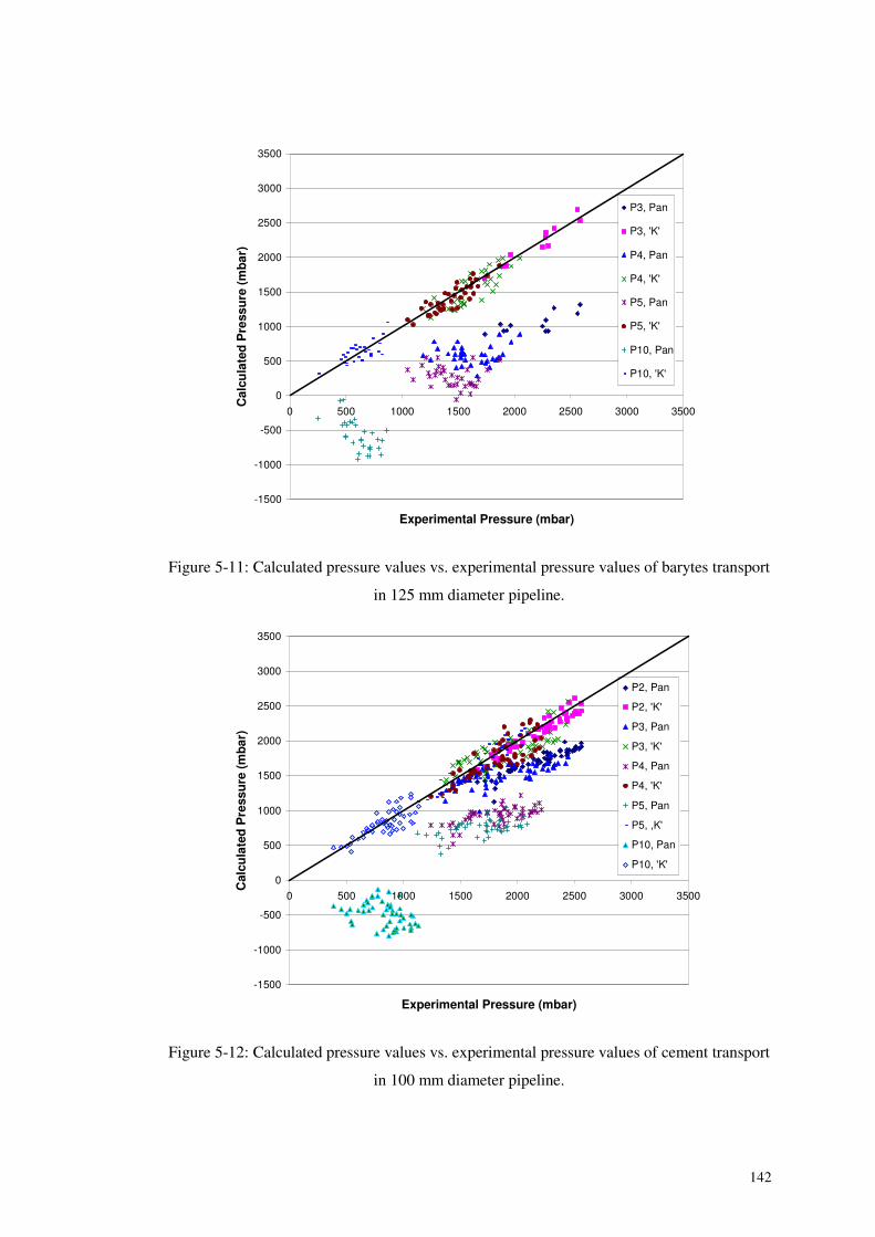
142
-1500
-1000
-500
0
500
1000
1500
2000
2500
3000
3500
0 500 1000 1500 2000 2500 3000 3500
Experimental Pressure (mbar)
Cal
cula
ted
Pre
ssu
re(m
bar
)
P3, Pan
P3, 'K'
P4, Pan
P4, 'K'
P5, Pan
P5, 'K'
P10, Pan
P10, 'K'
Figure 5-11: Calculated pressure values vs. experimental pressure values of barytes transport
in 125 mm diameter pipeline.
-1500
-1000
-500
0
500
1000
1500
2000
2500
3000
3500
0 500 1000 1500 2000 2500 3000 3500
Experimental Pressure (mbar)
Cal
cula
ted
Pre
ssu
re(m
bar
)
P2, Pan
P2, 'K'
P3, Pan
P3, 'K'
P4, Pan
P4, 'K'
P5, Pan
P5, ,K'
P10, Pan
P10, 'K'
Figure 5-12: Calculated pressure values vs. experimental pressure values of cement transport
in 100 mm diameter pipeline.
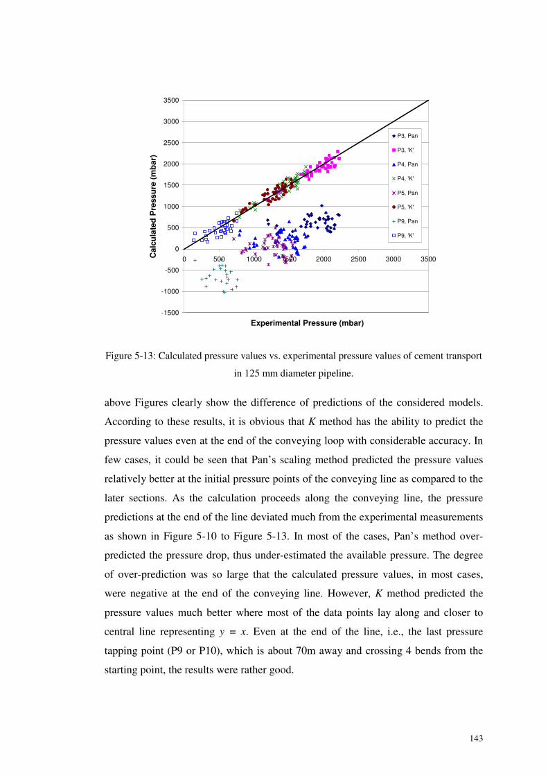
143
-1500
-1000
-500
0
500
1000
1500
2000
2500
3000
3500
0 500 1000 1500 2000 2500 3000 3500
Experimental Pressure (mbar)
Cal
cula
ted
Pre
ssu
re(m
bar
)
P3, Pan
P3, 'K'
P4, Pan
P4, 'K'
P5, Pan
P5, 'K'
P9, Pan
P9, 'K'
Figure 5-13: Calculated pressure values vs. experimental pressure values of cement transport
in 125 mm diameter pipeline.
above Figures clearly show the difference of predictions of the considered models.
According to these results, it is obvious that K method has the ability to predict the
pressure values even at the end of the conveying loop with considerable accuracy. In
few cases, it could be seen that Pan’s scaling method predicted the pressure values
relatively better at the initial pressure points of the conveying line as compared to the
later sections. As the calculation proceeds along the conveying line, the pressure
predictions at the end of the line deviated much from the experimental measurements
as shown in Figure 5-10 to Figure 5-13. In most of the cases, Pan’s method over-
predicted the pressure drop, thus under-estimated the available pressure. The degree
of over-prediction was so large that the calculated pressure values, in most cases,
were negative at the end of the conveying line. However, K method predicted the
pressure values much better where most of the data points lay along and closer to
central line representing y = x. Even at the end of the line, i.e., the last pressure
tapping point (P9 or P10), which is about 70m away and crossing 4 bends from the
starting point, the results were rather good.
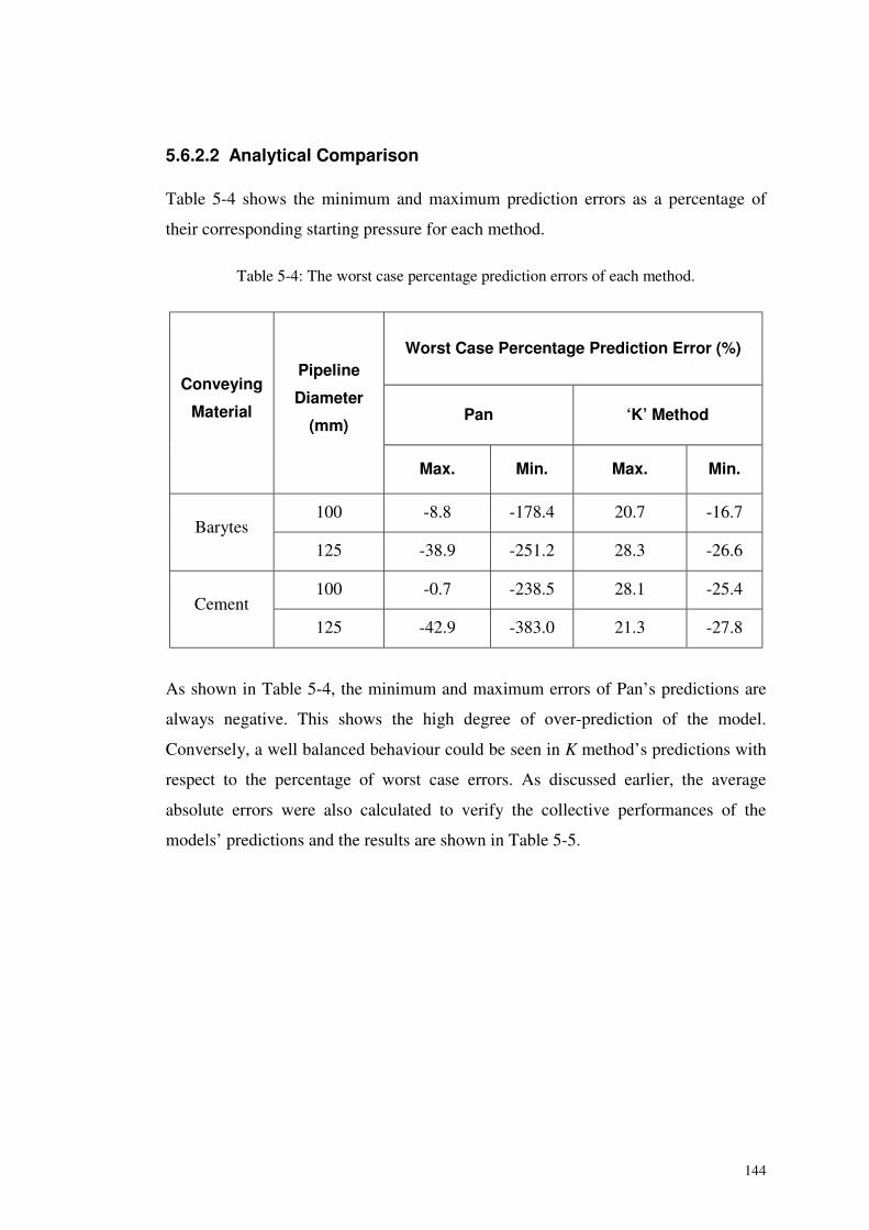
144
5.6.2.2 Analytical Comparison
Table 5-4 shows the minimum and maximum prediction errors as a percentage of
their corresponding starting pressure for each method.
Table 5-4: The worst case percentage prediction errors of each method.
Worst Case Percentage Prediction Error (%)
Pan ‘K’ Method
Conveying
Material
Pipeline
Diameter
(mm)
Max. Min. Max. Min.
100 -8.8 -178.4 20.7 -16.7Barytes
125 -38.9 -251.2 28.3 -26.6
100 -0.7 -238.5 28.1 -25.4Cement
125 -42.9 -383.0 21.3 -27.8
As shown in Table 5-4, the minimum and maximum errors of Pan’s predictions are
always negative. This shows the high degree of over-prediction of the model.
Conversely, a well balanced behaviour could be seen in K method’s predictions with
respect to the percentage of worst case errors. As discussed earlier, the average
absolute errors were also calculated to verify the collective performances of the
models’ predictions and the results are shown in Table 5-5.
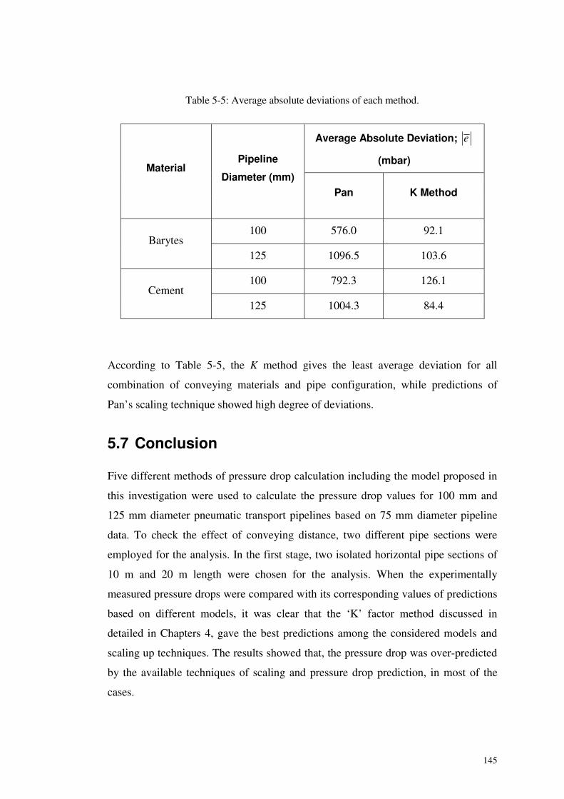
145
Table 5-5: Average absolute deviations of each method.
According to Table 5-5, the K method gives the least average deviation for all
combination of conveying materials and pipe configuration, while predictions of
Pan’s scaling technique showed high degree of deviations.
5.7 Conclusion
Five different methods of pressure drop calculation including the model proposed in
this investigation were used to calculate the pressure drop values for 100 mm and
125 mm diameter pneumatic transport pipelines based on 75 mm diameter pipeline
data. To check the effect of conveying distance, two different pipe sections were
employed for the analysis. In the first stage, two isolated horizontal pipe sections of
10 m and 20 m length were chosen for the analysis. When the experimentally
measured pressure drops were compared with its corresponding values of predictions
based on different models, it was clear that the ‘K’ factor method discussed in
detailed in Chapters 4, gave the best predictions among the considered models and
scaling up techniques. The results showed that, the pressure drop was over-predicted
by the available techniques of scaling and pressure drop prediction, in most of the
cases.
Average Absolute Deviation; e
(mbar)Material
Pipeline
Diameter (mm)Pan K Method
100 576.0 92.1Barytes
125 1096.5 103.6
100 792.3 126.1Cement
125 1004.3 84.4
146
In the second stage, the complete conveying loop was addressed with Pan’s and ‘K’
factor scaling up techniques. Taking the test results of 75 mm line as the basis, the
available pressure values at discrete positions of 100 mm and 125 mm lines were
calculated and compared with the actual pressures available at the same points.
Confirming the results of first stage, the ‘K’ factor method was identified as the
method, which gave the least percentage of error by analysing the results of second
stage. Specially, when the whole conveying loop including bends and other pipeline
accessories was considered, there was a risk of error accumulation of all other
methods, which lead to high discrepancies at the end of the conveying line. But, ‘K’
factor scaling technique was seen as a method that dealt this situation, satisfactorily.
147
6 PREDICTION OF PRESSURE DROP AT THEENTRY SECTION OF TOP DISCHARGEBLOW TANK
6.1 Introduction
As discussed in Chapter 2, in recent years, quite a lot of research papers have been
published on the topic of scaling up [16, 25, 42, 95, 101, 153], basically in two
distinguished categories; the global approach [16, 95, 153] and the piecewise
approach [25, 42, 101]. But, unfortunately, none of these methods addressed the
entry pressure loss i.e. the pressure drop across the feeding section of a top discharge
blow tank system. In fact, the entry pressure loss contributes to the total pressure
drop significantly. Especially, when the blow tank pressure has to be determined, this
component plays a vital role. Under the current investigation, a special attempt was
made to formulate a simple and straight forward scaling technique, which could be
used to determine the entry loss using the experimental data generated with different
bulk material. In this section, the back ground, model formulation and validation of
proposed scaling technique for entry pressure are discussed in detail.
6.2 Background
It is known that a blow tank has the interesting mechanism of self-regulation to
change the solid mass flow rate and mass loading ratio automatically, depending on
the conveying distance and on air pressure available in the tank. Rivkin [154]
explained this phenomena analogous to a closed-loop automatic control system,
where the conveying distance serves as feed back for the entrance to the conveying
line. He defined a threshold of the conveying distance, up to which this mechanism
seems to be valid (approximately 100 m) and this critical length is said to be
dependent upon the characteristics of the conveying bulk material such as particle
size, density, fluidizeability, etc. Lohrmann and Marcus [155, 156] studied the
performance of a bottom discharge blow tank with varying system parameters such
148
as line length, conveying velocity, etc. Jones et al. [33] compared the performance
differences between top and bottom discharge blow tanks and found that there is no
significant difference in the pressure, and thus the energy required to convey a
product through a pipeline at a given mass flow rate and loading condition in both
configurations. In a series of publications, Tomita et al. [157-162] explained the
performance and feed rate characteristics of a high pressure blow tank. Marjanovic
[163] formulated a model to predict the transient behaviour of a blow tank. But, none
have provided with any model to calculate the pressure loss incurred in the entry
section from a high pressure blow tank system.
With the aim of formulating a complete scaling up procedure, which can be applied
from initial point to end point of conveying system, a special attempt was made to
find a way of scaling up of the pressure loss at the entry section to pipeline
(henceforth called entry pressure loss) with the help of the experimental data. The
model has been formulated theoretically using dimensional analysis and later
validated with experimental data.
Under the current topic, the model formulation and validation results are presented in
details.
6.3 Test Setup
The details of the feeding section are shown in Figure 6-1.
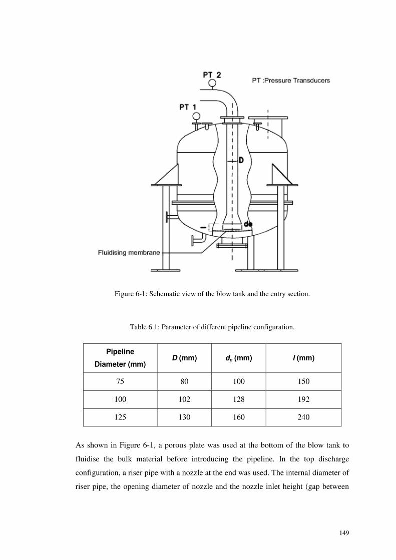
149
Figure 6-1: Schematic view of the blow tank and the entry section.
Table 6.1: Parameter of different pipeline configuration.
Pipeline
Diameter (mm)D (mm) de (mm) l (mm)
75 80 100 150
100 102 128 192
125 130 160 240
As shown in Figure 6-1, a porous plate was used at the bottom of the blow tank to
fluidise the bulk material before introducing the pipeline. In the top discharge
configuration, a riser pipe with a nozzle at the end was used. The internal diameter of
riser pipe, the opening diameter of nozzle and the nozzle inlet height (gap between
150
nozzle inlet and the porous plate) are labelled in Figure 6-1 as D, de and l
respectively and their nominal values for different pipeline configurations are given
in Table 6.1.
6.4 Details of Experiments
The data generated by the series of experiments described under the Section 4.5 were
utilised for the current investigation as well. Among the test materials for the main
investigation, only four bulk powders were selected for the current analysis. Barytes,
cement, ilmenite and five different qualities of alumina were chosen as the conveying
bulk materials. The properties and other relevant details of the test materials were
given in Chapter 4.
Under this investigation, a special attention was made on the entry section and the
pressure measurements and other readings relevant to entry section were taken into
consideration together with common measurements such as solids mass flow rate and
air volume flow rate.
6.5 Theoretical Approach
For this investigation, a well-known mathematical technique called dimensional
analysis [44, 164] has been used to derive a relationship between entry pressure loss
and the probable influencing parameters. The Buckingham � theorem, which is the
key theorem in dimensional analysis, states that the functional dependence between a
certain number (e.g.: n) of variables can be reduced by the number (e.g. m) of
independent dimensions occurring in those variables to give a set of p = n − m
independent, dimensionless numbers. A detailed description about the dimensional
analysis and the Buckingham � theorem is available in Ref.s [44, 164-166].
According to the standard procedure of dimensional analysis, the step wise approach
of model formulation is simply described in the following section.
151
6.5.1 List of influential parameter
Generally, the influential variables could be identified by considering few main
concepts, such as the geometry of the system, fluid properties involved with the
system and influential external effects of the system. According to this
categorization, the entry pressure loss can be considered as a function of a number of
pertinent variables:
1. Set pressure in blow tank (Ps)
2. Entry pressure loss (ΔPe)
3. Mass flow rate of solids (Ms)
4. Air volume flow rate (Qa)
5. Diameter of the riser tube (D)
6. Nozzle inlet height (l)
7. Particle density (ρs)
8. Particle mean diameter (dp)
9. Loading ratio (μ)
10. Entry diameter of the riser tube (de)
11. Air density (ρa)
Thus, the number of variables required to described the system could be found as 11
(n = 11; according to the usual notations).
6.5.2 Number of Dimensionless Groups Required
In the next step, the basic dimensions of the listed parameters were taken into
account. After checking the basic dimensions of the above variables, it was revealed
that all of them could be defined using three independent dimensions; e.i., M-mass,
L-length and T-time.
Thus, number of reference dimensions; m = 3.
According to the Buckingham � theorem, the number of dimensionless groups
required to describe the system could be determined as;
p = n –m
Therefore, p = 11 - 3 = 8
152
Then, the functional relationship among the still unknown dimensionless groups
could be presented as;
( )1 8,....., 0f Π Π = (6.1)
where, � i is a particular dimensionless combination of variables.
6.5.3 Determination of Repeating Variables
These repeating variables have to be selected from the original list of variables and
can be combined with each of the remaining variables to form � term. Few
conditions have to be satisfied when the repeating variables are selected [164]:
• All of the required reference dimensions must be included within the group of
repeating variables.
• The dimensions of one repeating variable cannot be reproduced by some
combination of products of powers of the remaining repeating variables (i.e.,
all repeating variable must be dimensionally independent of each other).
• The repeating variables cannot themselves be combined to form a
dimensionless product.
As its name implies, the repeating variables will generally appear in more than one �
term. Thus, from the above listed parameters, three parameters were selected as the
basic variables to combine with the rest of variables to form the required number of
dimensionless groups. Usually, the number of repeating variables required is equal to
the number of reference dimensions.
In this model formulation, few different combinations of repeating variables were
tried. According to the outcome of those different combinations, finally ΔPe, Ms and
D were selected as the repeating variables, since this combination of variables was
the best to satisfy the conditions of selections of repeating variable as mentioned in
Ref. [164].
153
6.5.4 Formation of Dimensionless Groups
The general procedure of formulation of a typical � term can be presented in the
following equation.
1 2 3i i ia b c
i iu u u uΠ = (6.2)
where; ui is one of the non-repeating variables
u1, u2 and u3 are the repeating variables
ai, bi and ci are the exponents
These exponents to the repeating variables are determined so that the combination is
dimensionless.
6.5.4.1 A Specimen Simplification
The following simplification presents the usual way of determination of a
dimensionless group (or a � term), as a specimen calculation.
The selected repeating variables: ΔPe, Ms and D
Consider ρs as the non-repeating variable and term the dimensionless number as �1;
According to equation (6.2),
( ) ( ) ( )1 1 1
1
a b c
s e sP M DρΠ = Δ (6.3)
Considering the basic dimensions of each term;
( ) ( )( ) ( ) ( )1 1 10 0 0 3 1 2 1a b cM L T ML ML T MT L− − − −≡ (6.4)
Equating the exponents of each of basic dimensions;
M: 1 11 0a b+ + = (6.5)
L: 1 13 0a c− − + = (6.6)
T: 1 12 0a b− − = (6.7)
Simplifying equations (6.5), (6.6) and (6.7), the values of exponents could be
determined as;
1
1
1
1
2
4
a
b
c
== −=
(6.8)
154
Equation (6.3) could then be rewritten as;
( )( ) ( )2 4
1 s e sP M Dρ −Π = Δ (6.9)
By rearranging the equation (6.9);
4
1 2e s
s
P D
M
ρΔΠ = (6.10)
Following the same procedure, the rest of the � groups could also be found and the
list of all � terms is given below.
4
1 2e s
s
P D
M
ρΔΠ = (6.11)
2s
e
P
PΠ =
Δ(6.12)
3 4s a
e
M Q
P DΠ =
Δ(6.13)
4
4 2e a
s
P D
M
ρΔΠ = (6.14)
5
l
DΠ = (6.15)
6pd
DΠ = (6.16)
7ed
DΠ = (6.17)
8 μΠ = (6.18)
6.5.5 Final Form of Functional Relationship
Putting them all together, the final set of � groups could be shown as below;
4 4
2 4 2, , , , , , , 0pe s s s a e a e
s e e s
dP D P M Q P D dlf
M P P D M D D D
ρ ρ μ� �Δ Δ =� �Δ Δ� �
(6.19)
Equation (6.19) could be manipulated further to the following form.
, , , , , , , 0e s p a ps s e
s s e a e
P d Q dP dl lf
P M D P d D D D
ρ ρ μρ
Δ� �=� �Δ� �
(6.20)
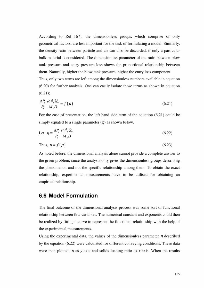
155
According to Ref.[167], the dimensionless groups, which comprise of only
geometrical factors, are less important for the task of formulating a model. Similarly,
the density ratio between particle and air can also be discarded, if only a particular
bulk material is considered. The dimensionless parameter of the ratio between blow
tank pressure and entry pressure loss shows the proportional relationship between
them. Naturally, higher the blow tank pressure, higher the entry loss component.
Thus, only two terms are left among the dimensionless numbers available in equation
(6.20) for further analysis. One can easily isolate those terms as shown in equation
(6.21);
( )s p ae
s s
d QPf
P M D
ρμΔ = (6.21)
For the ease of presentation, the left hand side term of the equation (6.21) could be
simply equated to a single parameter (η) as shown below.
Let, s p ae
s s
d QP
P M D
ρη Δ≡ (6.22)
Thus, ( )fη μ= (6.23)
As noted before, the dimensional analysis alone cannot provide a complete answer to
the given problem, since the analysis only gives the dimensionless groups describing
the phenomenon and not the specific relationship among them. To obtain the exact
relationship, experimental measurements have to be utilised for obtaining an
empirical relationship.
6.6 Model Formulation
The final outcome of the dimensional analysis process was some sort of functional
relationship between few variables. The numerical constant and exponents could then
be realized by fitting a curve to represent the functional relationship with the help of
the experimental measurements.
Using the experimental data, the values of the dimensionless parameter η described
by the equation (6.22) were calculated for different conveying conditions. These data
were then plotted; η as y-axis and solids loading ratio as x-axis. When the results
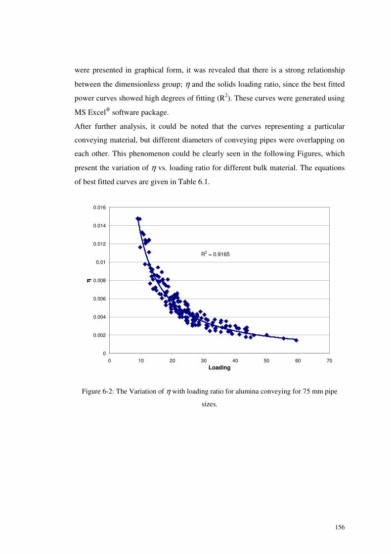
156
were presented in graphical form, it was revealed that there is a strong relationship
between the dimensionless group; η and the solids loading ratio, since the best fitted
power curves showed high degrees of fitting (R2). These curves were generated using
MS Excel® software package.
After further analysis, it could be noted that the curves representing a particular
conveying material, but different diameters of conveying pipes were overlapping on
each other. This phenomenon could be clearly seen in the following Figures, which
present the variation of η vs. loading ratio for different bulk material. The equations
of best fitted curves are given in Table 6.1.
R2 = 0.9165
0
0.002
0.004
0.006
0.008
0.01
0.012
0.014
0.016
0 10 20 30 40 50 60 70Loading
ηη ηη
Figure 6-2: The Variation of η with loading ratio for alumina conveying for 75 mm pipe
sizes.
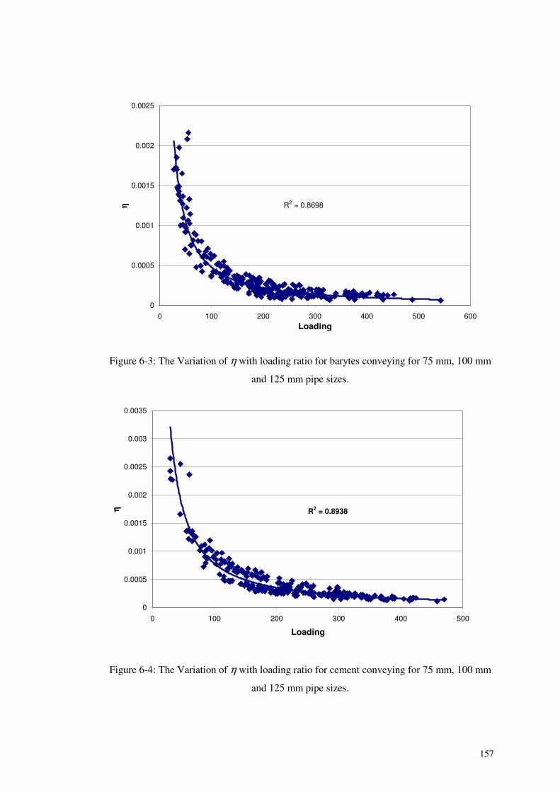
157
R2 = 0.8698
0
0.0005
0.001
0.0015
0.002
0.0025
0 100 200 300 400 500 600Loading
ηη ηη
Figure 6-3: The Variation of η with loading ratio for barytes conveying for 75 mm, 100 mm
and 125 mm pipe sizes.
R2 = 0.8938
0
0.0005
0.001
0.0015
0.002
0.0025
0.003
0.0035
0 100 200 300 400 500
Loading
ηη ηη
Figure 6-4: The Variation of η with loading ratio for cement conveying for 75 mm, 100 mm
and 125 mm pipe sizes.
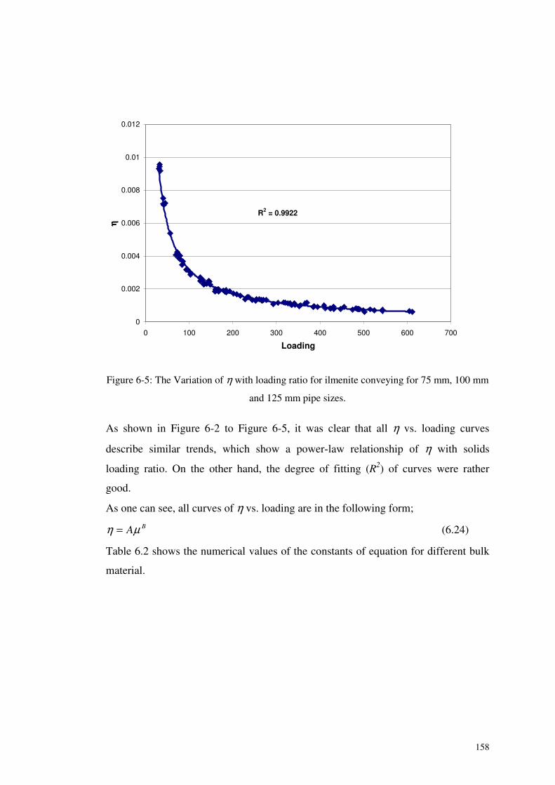
158
R2 = 0.9922
0
0.002
0.004
0.006
0.008
0.01
0.012
0 100 200 300 400 500 600 700
Loading
ηη ηη
Figure 6-5: The Variation of η with loading ratio for ilmenite conveying for 75 mm, 100 mm
and 125 mm pipe sizes.
As shown in Figure 6-2 to Figure 6-5, it was clear that all η vs. loading curves
describe similar trends, which show a power-law relationship of η with solids
loading ratio. On the other hand, the degree of fitting (R2) of curves were rather
good.
As one can see, all curves of η vs. loading are in the following form;
BAμη = (6.24)
Table 6.2 shows the numerical values of the constants of equation for different bulk
material.
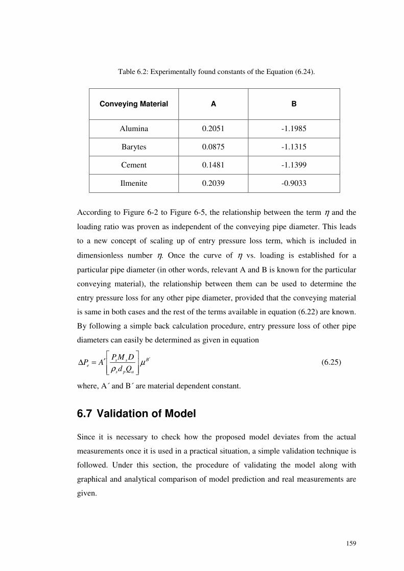
159
Table 6.2: Experimentally found constants of the Equation (6.24).
Conveying Material A B
Alumina 0.2051 -1.1985
Barytes 0.0875 -1.1315
Cement 0.1481 -1.1399
Ilmenite 0.2039 -0.9033
According to Figure 6-2 to Figure 6-5, the relationship between the term η and the
loading ratio was proven as independent of the conveying pipe diameter. This leads
to a new concept of scaling up of entry pressure loss term, which is included in
dimensionless number η. Once the curve of η vs. loading is established for a
particular pipe diameter (in other words, relevant A and B is known for the particular
conveying material), the relationship between them can be used to determine the
entry pressure loss for any other pipe diameter, provided that the conveying material
is same in both cases and the rest of the terms available in equation (6.22) are known.
By following a simple back calculation procedure, entry pressure loss of other pipe
diameters can easily be determined as given in equation
Bs se
s p a
P M DP A
d Qμ
ρ′� �
′Δ = � �� �� �
(6.25)
where, A´ and B´ are material dependent constant.
6.7 Validation of Model
Since it is necessary to check how the proposed model deviates from the actual
measurements once it is used in a practical situation, a simple validation technique is
followed. Under this section, the procedure of validating the model along with
graphical and analytical comparison of model prediction and real measurements are
given.
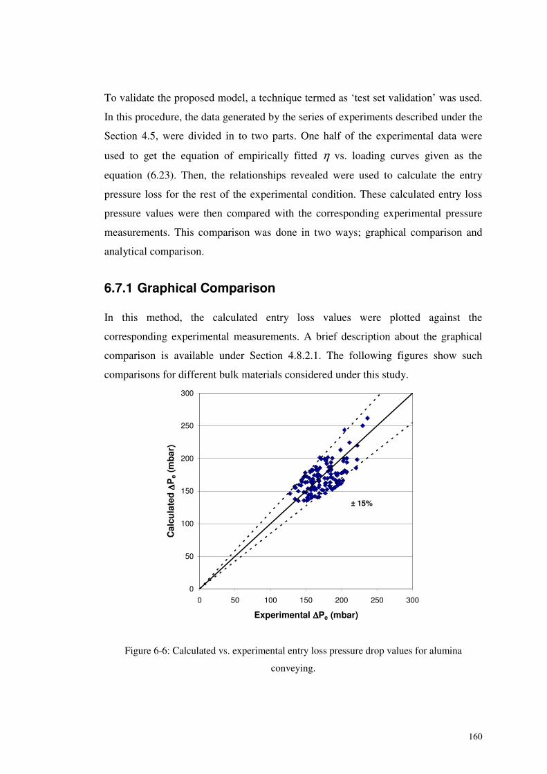
160
To validate the proposed model, a technique termed as ‘test set validation’ was used.
In this procedure, the data generated by the series of experiments described under the
Section 4.5, were divided in to two parts. One half of the experimental data were
used to get the equation of empirically fitted η vs. loading curves given as the
equation (6.23). Then, the relationships revealed were used to calculate the entry
pressure loss for the rest of the experimental condition. These calculated entry loss
pressure values were then compared with the corresponding experimental pressure
measurements. This comparison was done in two ways; graphical comparison and
analytical comparison.
6.7.1 Graphical Comparison
In this method, the calculated entry loss values were plotted against the
corresponding experimental measurements. A brief description about the graphical
comparison is available under Section 4.8.2.1. The following figures show such
comparisons for different bulk materials considered under this study.
0
50
100
150
200
250
300
0 50 100 150 200 250 300
Experimental ΔΔΔΔPe (mbar)
Cal
cula
tedΔΔ ΔΔ
Pe
(mb
ar)
± 15%
Figure 6-6: Calculated vs. experimental entry loss pressure drop values for alumina
conveying.
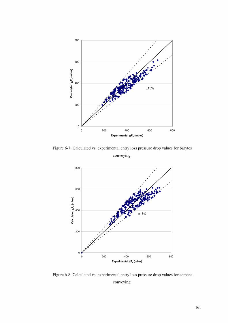
161
0
200
400
600
800
0 200 400 600 800
Experimental ΔΔΔΔPe (mbar)
Cal
cula
tedΔΔ ΔΔ
Pe
(mb
ar)
±15%
Figure 6-7: Calculated vs. experimental entry loss pressure drop values for barytes
conveying.
0
200
400
600
800
0 200 400 600 800
Experimental ΔΔΔΔPe (mbar)
Cal
cula
tedΔΔ ΔΔ
Pe
(mb
ar)
±15%
Figure 6-8: Calculated vs. experimental entry loss pressure drop values for cement
conveying.
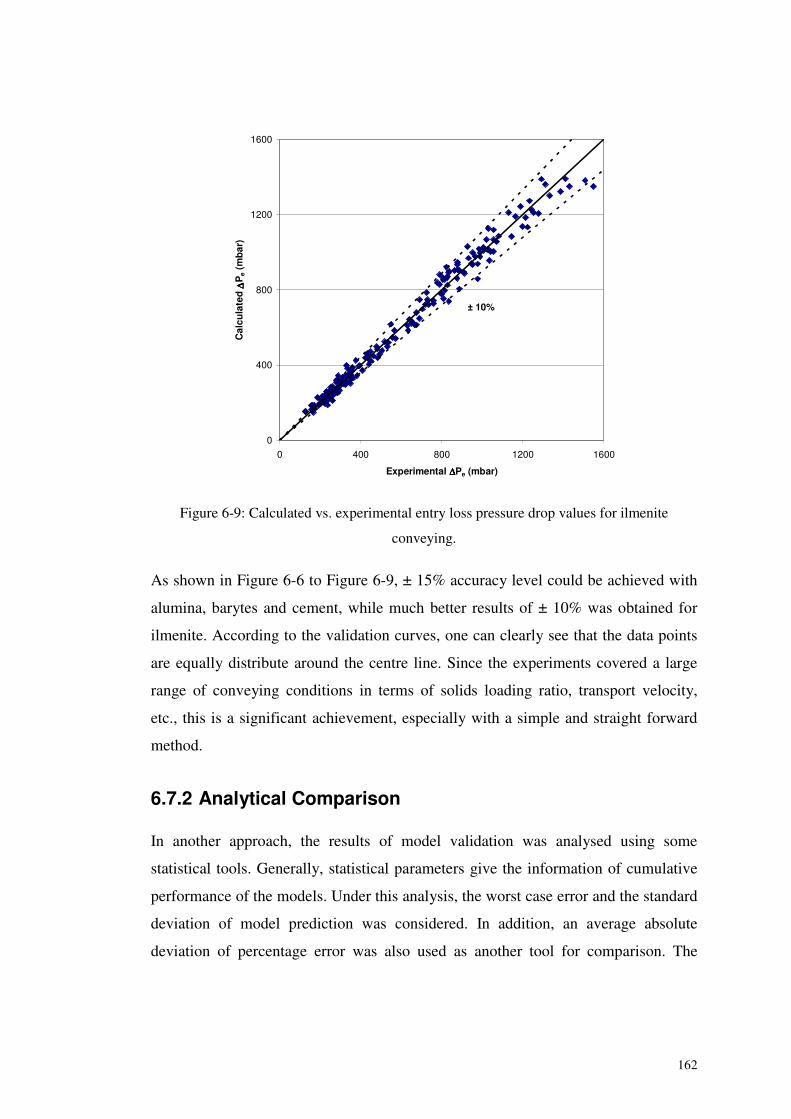
162
0
400
800
1200
1600
0 400 800 1200 1600
Experimental ΔΔΔΔPe (mbar)
Cal
cula
tedΔΔ ΔΔ
Pe
(mb
ar)
± 10%
Figure 6-9: Calculated vs. experimental entry loss pressure drop values for ilmenite
conveying.
As shown in Figure 6-6 to Figure 6-9, ± 15% accuracy level could be achieved with
alumina, barytes and cement, while much better results of ± 10% was obtained for
ilmenite. According to the validation curves, one can clearly see that the data points
are equally distribute around the centre line. Since the experiments covered a large
range of conveying conditions in terms of solids loading ratio, transport velocity,
etc., this is a significant achievement, especially with a simple and straight forward
method.
6.7.2 Analytical Comparison
In another approach, the results of model validation was analysed using some
statistical tools. Generally, statistical parameters give the information of cumulative
performance of the models. Under this analysis, the worst case error and the standard
deviation of model prediction was considered. In addition, an average absolute
deviation of percentage error was also used as another tool for comparison. The
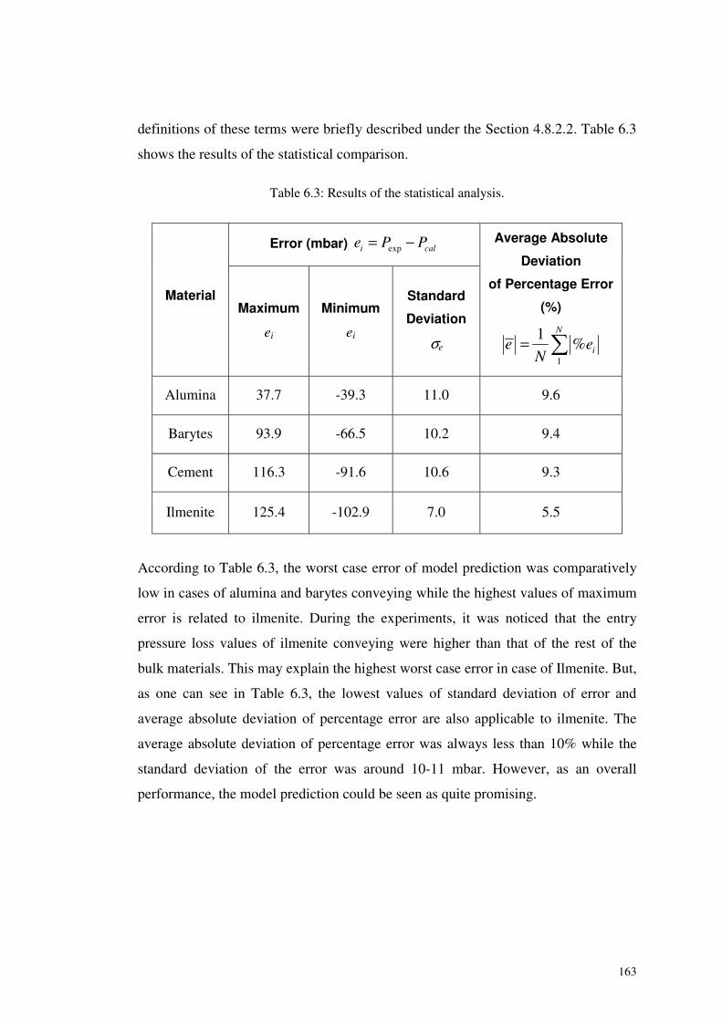
163
definitions of these terms were briefly described under the Section 4.8.2.2. Table 6.3
shows the results of the statistical comparison.
Table 6.3: Results of the statistical analysis.
According to Table 6.3, the worst case error of model prediction was comparatively
low in cases of alumina and barytes conveying while the highest values of maximum
error is related to ilmenite. During the experiments, it was noticed that the entry
pressure loss values of ilmenite conveying were higher than that of the rest of the
bulk materials. This may explain the highest worst case error in case of Ilmenite. But,
as one can see in Table 6.3, the lowest values of standard deviation of error and
average absolute deviation of percentage error are also applicable to ilmenite. The
average absolute deviation of percentage error was always less than 10% while the
standard deviation of the error was around 10-11 mbar. However, as an overall
performance, the model prediction could be seen as quite promising.
Error (mbar) expi cale P P= −
MaterialMaximum
ei
Minimum
ei
Standard
Deviation
σe
Average Absolute
Deviation
of Percentage Error
(%)
1
1%
N
ie eN
= �
Alumina 37.7 -39.3 11.0 9.6
Barytes 93.9 -66.5 10.2 9.4
Cement 116.3 -91.6 10.6 9.3
Ilmenite 125.4 -102.9 7.0 5.5
164
6.8 Conclusion
The model for prediction of entry pressure loss in a top discharge blow tank
situation, derived using dimensional analysis promises to be a very useful and
reliable scaling up tool, which can be used in conjunction with the pressure drop
prediction technique proposed in Chapter 4. The predicted values of entry pressure
loss agree well with the experimental data. The model proposed here is very simple
and needs only readily available experimental data without any complicated
manipulation.
165
7 SCALING UP OF MINIMUM CONVEYINGCONDITIONS IN A PNEUMATIC TRANSPORTSYSTEM
7.1 Introduction
The minimum conveying air velocity is one of the key parameters in the pneumatic
transport of particulate bulk materials. An unnecessarily high conveying velocity will
result in higher energy costs due to an increased pressure drop in the system, solids
degradation, and pipe erosion that can result in an economically unattractive
operation. On the other hand, systems designed with extremely low conveying
velocities or extremely high solid flow rates are subject to erratic operation due to
solids disposition or they may be completely inoperable because of blocking.
Keeping gas velocity above minimum conveying velocity in all horizontal sections of
a pipeline ensures no deposition of solids in the system and a continuous, safe and
steady transport.
According to the description under Section 2, it was clear that many terms have been
used to refer to minimum conveying velocity by researchers and designers of
pneumatic conveying systems, over the years. Among them, minimum transport
velocity [37, 168], saltation velocity [14, 34, 35, 89, 169], pickup velocity [34, 35,
89], critical velocity [170, 171], velocity at the pressure minimum point of the
general state diagram [37, 39], stability limit [69], etc., are popular terminologies to
define the lowest safe gas velocity to convey the particulate materials in a pipe
system. Definitions of these terms are based on visual observations and pressure drop
measurements, and they are often applied to indicate some transition in the way, in
which the particles are moving or begin to move.
Although quite a few scaling up techniques [16, 25, 42, 95, 101] are available in the
literature, there still remain some doubt whether they address the important issues of
the minimum conveying velocity properly. Specially, after the findings of few
researchers, like Yi et al. [172], it has been revealed that the existing models are not
166
good enough to address the conveying of fine bulk materials. In a review paper, Yi et
al. [172] evaluated the influence of particle properties, pipeline configuration and
conveying conditions on minimum conveying velocity by comparing 11
recommended correlations. They found that the predictions showed quite different
trends for variations in particle diameter, particle density, gas density, gas viscosity
and temperature. In case of fine bulk materials (<100 μm approximately), the scatter
in the predicted values was so significant that they could not provide any reliable
minimum conveying velocity for industrial application. Hence there exists a need for
developing a technique for prediction of minimum conveying velocity for such bulk
powders.
In the process of formulating a complete scaling technique, a special attention was
paid to formulate a model to scale up the minimum conveying condition together
with other important issues like conveying line pressure drop and entry section
pressure drop discussed in earlier Chapters 4 and 6.
This chapter presents the results and findings of the investigation on minimum
conveying velocity with respect to different bulk materials conveyed in different pipe
configurations. In addition, the performance of the proposed model was compared
with some other correlations, which could readily be used in scaling up and
determination of minimum conveying velocities. Four materials including one with
five different qualities have been tested in four different pipeline configurations with
respect to pipe length and diameter.
7.2 Background
The literature survey described under the Chapter 2 revealed that numerous
theoretical and empirical correlations [14, 34-38, 89, 90, 94, 146, 168-171, 173-183]
have been developed for the prediction of minimum conveying velocity. Some of
them [34, 35, 89, 180] require particular information about the single particle
behaviours, which needs special experimental measurements. On the other hand,
some correlations [14, 171] need graphically determined parameters. Similarly, some
correlations [170, 171, 179, 181] are based on parameters, which do not have
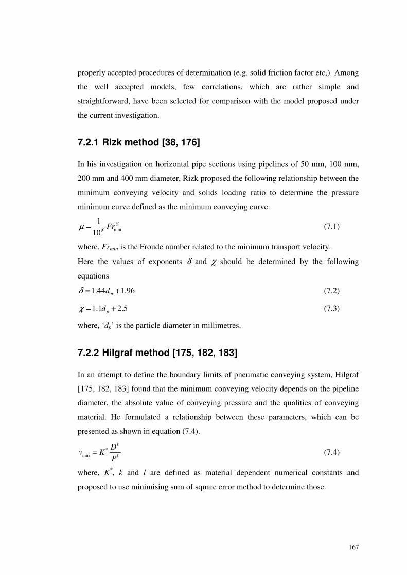
167
properly accepted procedures of determination (e.g. solid friction factor etc,). Among
the well accepted models, few correlations, which are rather simple and
straightforward, have been selected for comparison with the model proposed under
the current investigation.
7.2.1 Rizk method [38, 176]
In his investigation on horizontal pipe sections using pipelines of 50 mm, 100 mm,
200 mm and 400 mm diameter, Rizk proposed the following relationship between the
minimum conveying velocity and solids loading ratio to determine the pressure
minimum curve defined as the minimum conveying curve.
min
1
10Fr χδμ = (7.1)
where, Frmin is the Froude number related to the minimum transport velocity.
Here the values of exponents δ and χ should be determined by the following
equations
1.44 1.96pdδ = + (7.2)
1.1 2.5pdχ = + (7.3)
where, ‘dp’ is the particle diameter in millimetres.
7.2.2 Hilgraf method [175, 182, 183]
In an attempt to define the boundary limits of pneumatic conveying system, Hilgraf
[175, 182, 183] found that the minimum conveying velocity depends on the pipeline
diameter, the absolute value of conveying pressure and the qualities of conveying
material. He formulated a relationship between these parameters, which can be
presented as shown in equation (7.4).
*min
k
l
Dv K
P= (7.4)
where, K*, k and l are defined as material dependent numerical constants and
proposed to use minimising sum of square error method to determine those.
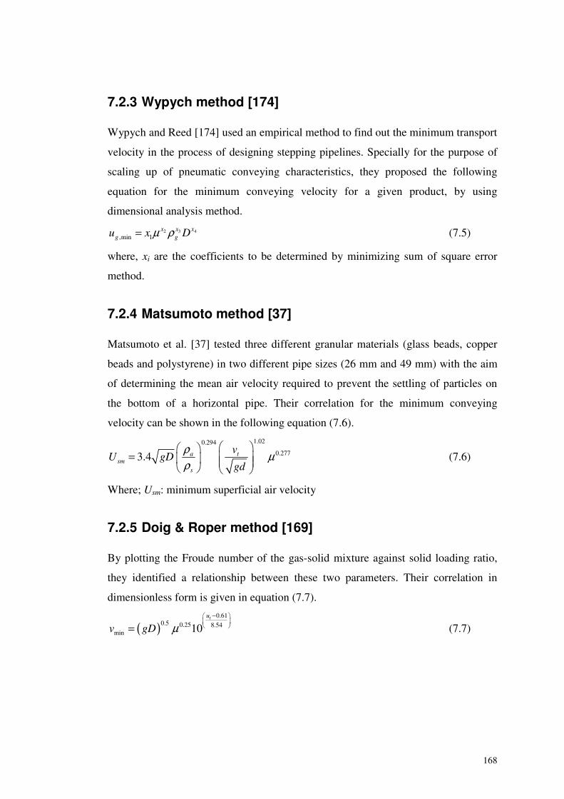
168
7.2.3 Wypych method [174]
Wypych and Reed [174] used an empirical method to find out the minimum transport
velocity in the process of designing stepping pipelines. Specially for the purpose of
scaling up of pneumatic conveying characteristics, they proposed the following
equation for the minimum conveying velocity for a given product, by using
dimensional analysis method.
32 4,min 1
xx xg gu x Dμ ρ= (7.5)
where, xi are the coefficients to be determined by minimizing sum of square error
method.
7.2.4 Matsumoto method [37]
Matsumoto et al. [37] tested three different granular materials (glass beads, copper
beads and polystyrene) in two different pipe sizes (26 mm and 49 mm) with the aim
of determining the mean air velocity required to prevent the settling of particles on
the bottom of a horizontal pipe. Their correlation for the minimum conveying
velocity can be shown in the following equation (7.6).
1.020.294
0.2773.4 a tsm
s
vU gD
gd
ρ μρ
= � �� � � �� �
(7.6)
Where; Usm: minimum superficial air velocity
7.2.5 Doig & Roper method [169]
By plotting the Froude number of the gas-solid mixture against solid loading ratio,
they identified a relationship between these two parameters. Their correlation in
dimensionless form is given in equation (7.7).
( )0.61
0.5 0.25 8.54min 10
tu
v gD μ−
� �� = (7.7)
169
7.2.6 Martinussen’s model [36]
Martinussen [36] used experimental set-up of 15m long horizontal pipeline with 53
mm bore. The fluid analogy was applied to develop a model for the prediction of
when blockage will occur in pipeline and a model was proposed to determine the
minimum conveying velocity.
3
2min 1b a
a b
v KDgρ ρμρ ρ
� �= −� �
� �(7.8)
where K; geometrical factor = π/4 at the filling level of D/2. This gives better
predictions for fine materials since the effect of the permeability has not been
included.
7.3 Test Setup and Material
As explained under the section 7.1, this investigation was carried out as a part of the
main task to formulate a complete scaling technique for the pneumatic conveying
system design.
7.4 Theoretical Consideration
The main objective of this work is to formulate a possible scaling up procedure for
the minimum conveying boundary that can be graphically shown in typical
pneumatic conveying characteristics as shown in Figure 7-1.
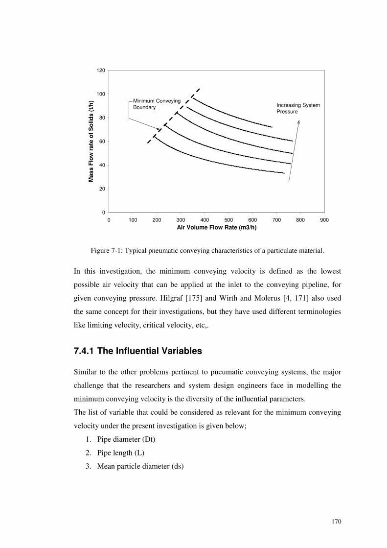
170
0
20
40
60
80
100
120
0 100 200 300 400 500 600 700 800 900
Air Volume Flow Rate (m3/h)
Mas
sF
low
rate
of
So
lids
(t/h
) Minimum ConveyingBoundary Increasing System
Pressure
Figure 7-1: Typical pneumatic conveying characteristics of a particulate material.
In this investigation, the minimum conveying velocity is defined as the lowest
possible air velocity that can be applied at the inlet to the conveying pipeline, for
given conveying pressure. Hilgraf [175] and Wirth and Molerus [4, 171] also used
the same concept for their investigations, but they have used different terminologies
like limiting velocity, critical velocity, etc,.
7.4.1 The Influential Variables
Similar to the other problems pertinent to pneumatic conveying systems, the major
challenge that the researchers and system design engineers face in modelling the
minimum conveying velocity is the diversity of the influential parameters.
The list of variable that could be considered as relevant for the minimum conveying
velocity under the present investigation is given below;
1. Pipe diameter (Dt)
2. Pipe length (L)
3. Mean particle diameter (ds)
171
4. Particle density (Rhos)
5. Solids mass flow rate (Ms)
6. Air volume flow rate (Ma)
7. Density of air (Rhoa)
8. Solids loading ratio (SLR)
9. Blow tank pressure (BTP)
For the convenience of referring the variables in later data analysis stages, the
notations corresponding to each variable (given in parenthesis) will be used. In the
model formulation, there are, basically, three major steps as listed below;
1. Screening of relevant physical characteristics, using a mathematical tool
called ‘Principal Component Analysis (PCA)’ described in multivariate data
analysis [184]
2. Use of the concept of dimensional analysis [164, 166] to formulate a
functional relationship between the most important parameters.
3. Utilising the experimental measurements to establish the exact relationship.
7.4.2 Use of Multivariate Data Analysis
‘Principal Component Analysis (PCA)’ is a multivariate statistical procedure that
transforms a number of correlated variables into a smaller number of uncorrelated
new variables called ‘Principal Components (PC)’. The concept of principal
component is also used in regression methodology in same line as Multiple Linear
Regression (MLR). This regression technique is generally termed as ‘Partial Least
Squares Regression (PLS-R)’ or in popular terminology ‘PLS’, which has also been
interpreted as ‘Projection to Latent Structures’. These tools and concepts are
described in Ref. [184], in details.
However, PLS technique facilitates to identify the ‘Loading Weights’ of independent
variable in the process of building a regression relationship between dependent and
independent variables. These loading weights could be graphically represented in
terms of considered principal components. Each independent variable has a loading
weight along each model component. All the data analysis operations in the present
172
investigation were carried out with the help of a software package called ‘The
Unscrabler®’ [184].
The loading weights describe how much each variable contributes to explaining the
response variation along each model component. Generally, they can be used to
represent the relationship between independent and dependent variables. These
loading weight plots could be easily used to identify the most important variables
among all other assumed parameters at the starting of model formulation. A similar
technique could be seen in Ref. [185] where these data analysis tools were
effectively used for variable reduction in model formulation.
7.4.3 Data Analysis Trials
Few simple multivariate data analysis trials were carried out with the help of the
Unscrabler® using experimental data. In this stage, the experimental observations
relevant to a particular conveying material were chosen for the preliminary data
analysis process.
Initially, the experimental measurements of the variables listed under section 7.4.1
were taken into account together with the corresponding velocity values. Special
attention was paid to consider the data relevant to extreme conveying conditions,
which correspond to minimum conveying air flow rate or the maximum solids
loading conditions. It is reasonable to take these observations as the experimental
data applicable to minimum conveying condition, since special care was taken during
the tests to obtain the lowest possible conveying air flow rates, which were nearly the
blocking limits of each conveying materials.
7.4.3.1 PCA
Initially, the experimental data were tested with PCA technique to find out the
required number of PC to explain most of the information of the considered problem.
It could be noticed that the data relevant to different materials behaved in almost
similar way in PCA testing. For the convenience of presentation, the results of
cement data are only given and described.
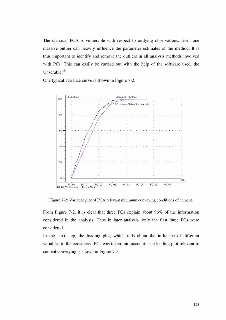
173
The classical PCA is vulnerable with respect to outlying observations. Even one
massive outlier can heavily influence the parameter estimates of the method. It is
thus important to identify and remove the outliers in all analysis methods involved
with PCs. This can easily be carried out with the help of the software used, the
Unscrabler®.
One typical variance curve is shown in Figure 7-2.
Figure 7-2: Variance plot of PCA relevant minimum conveying conditions of cement.
From Figure 7-2, it is clear that three PCs explain about 96% of the information
considered in the analysis. Thus in later analysis, only the first three PCs were
considered.
In the next step, the loading plot, which tells about the influence of different
variables to the considered PCs was taken into account. The loading plot relevant to
cement conveying is shown in Figure 7-3.
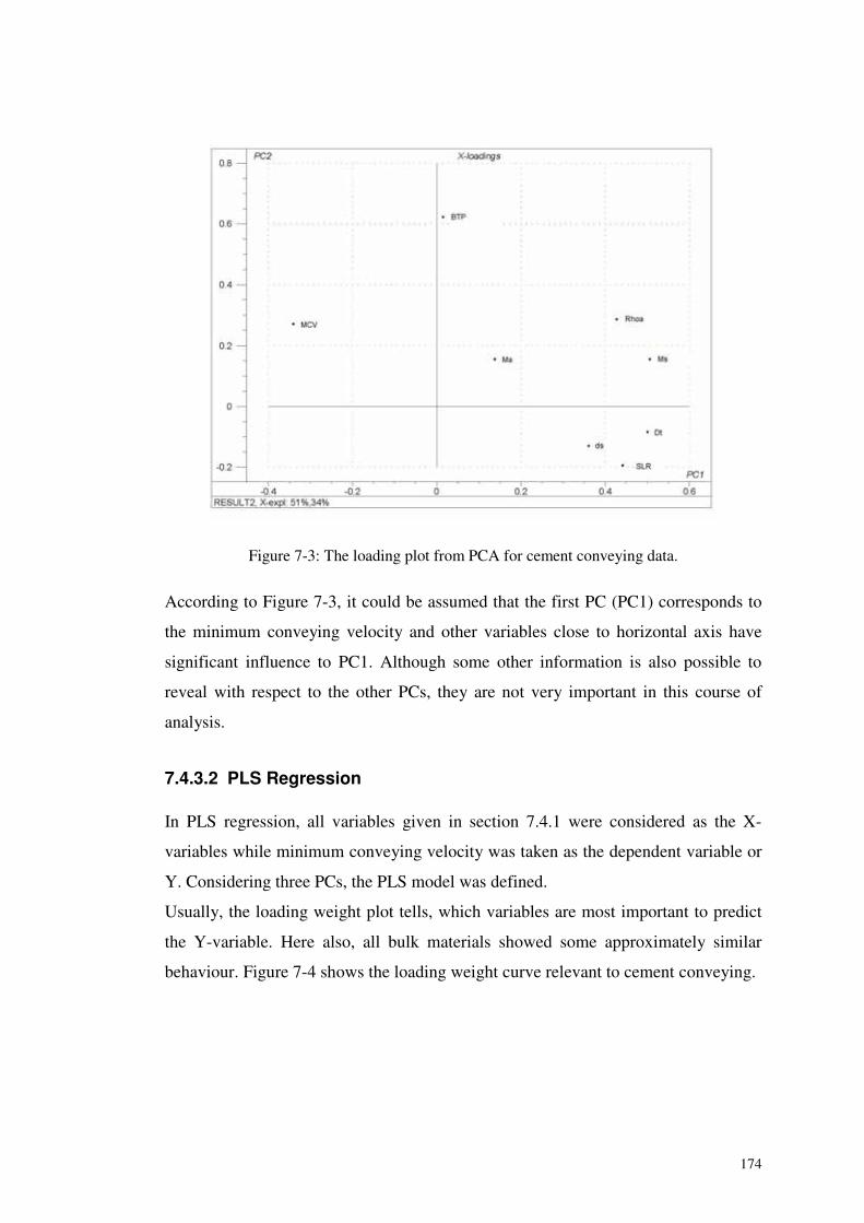
174
Figure 7-3: The loading plot from PCA for cement conveying data.
According to Figure 7-3, it could be assumed that the first PC (PC1) corresponds to
the minimum conveying velocity and other variables close to horizontal axis have
significant influence to PC1. Although some other information is also possible to
reveal with respect to the other PCs, they are not very important in this course of
analysis.
7.4.3.2 PLS Regression
In PLS regression, all variables given in section 7.4.1 were considered as the X-
variables while minimum conveying velocity was taken as the dependent variable or
Y. Considering three PCs, the PLS model was defined.
Usually, the loading weight plot tells, which variables are most important to predict
the Y-variable. Here also, all bulk materials showed some approximately similar
behaviour. Figure 7-4 shows the loading weight curve relevant to cement conveying.
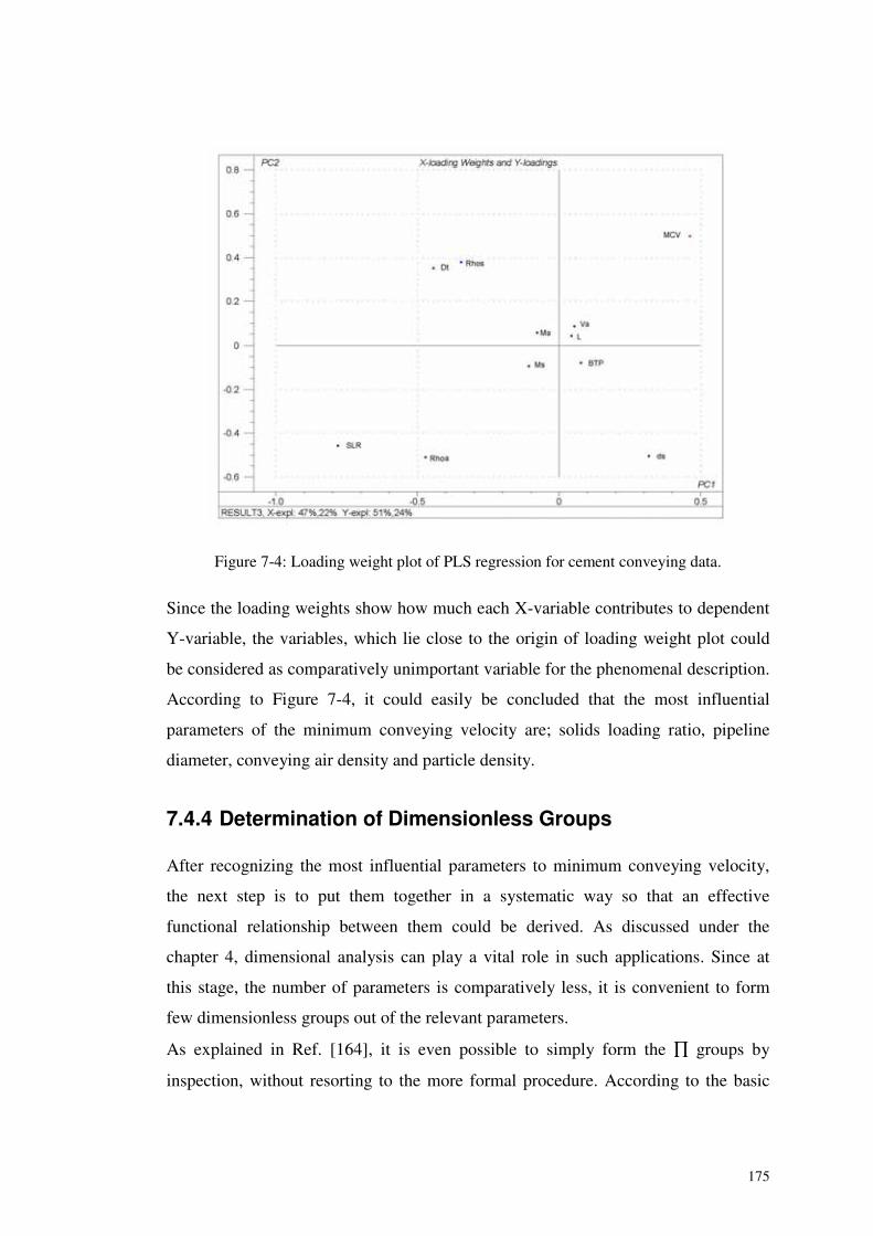
175
Figure 7-4: Loading weight plot of PLS regression for cement conveying data.
Since the loading weights show how much each X-variable contributes to dependent
Y-variable, the variables, which lie close to the origin of loading weight plot could
be considered as comparatively unimportant variable for the phenomenal description.
According to Figure 7-4, it could easily be concluded that the most influential
parameters of the minimum conveying velocity are; solids loading ratio, pipeline
diameter, conveying air density and particle density.
7.4.4 Determination of Dimensionless Groups
After recognizing the most influential parameters to minimum conveying velocity,
the next step is to put them together in a systematic way so that an effective
functional relationship between them could be derived. As discussed under the
chapter 4, dimensional analysis can play a vital role in such applications. Since at
this stage, the number of parameters is comparatively less, it is convenient to form
few dimensionless groups out of the relevant parameters.
As explained in Ref. [164], it is even possible to simply form the ∏ groups by
inspection, without resorting to the more formal procedure. According to the basic
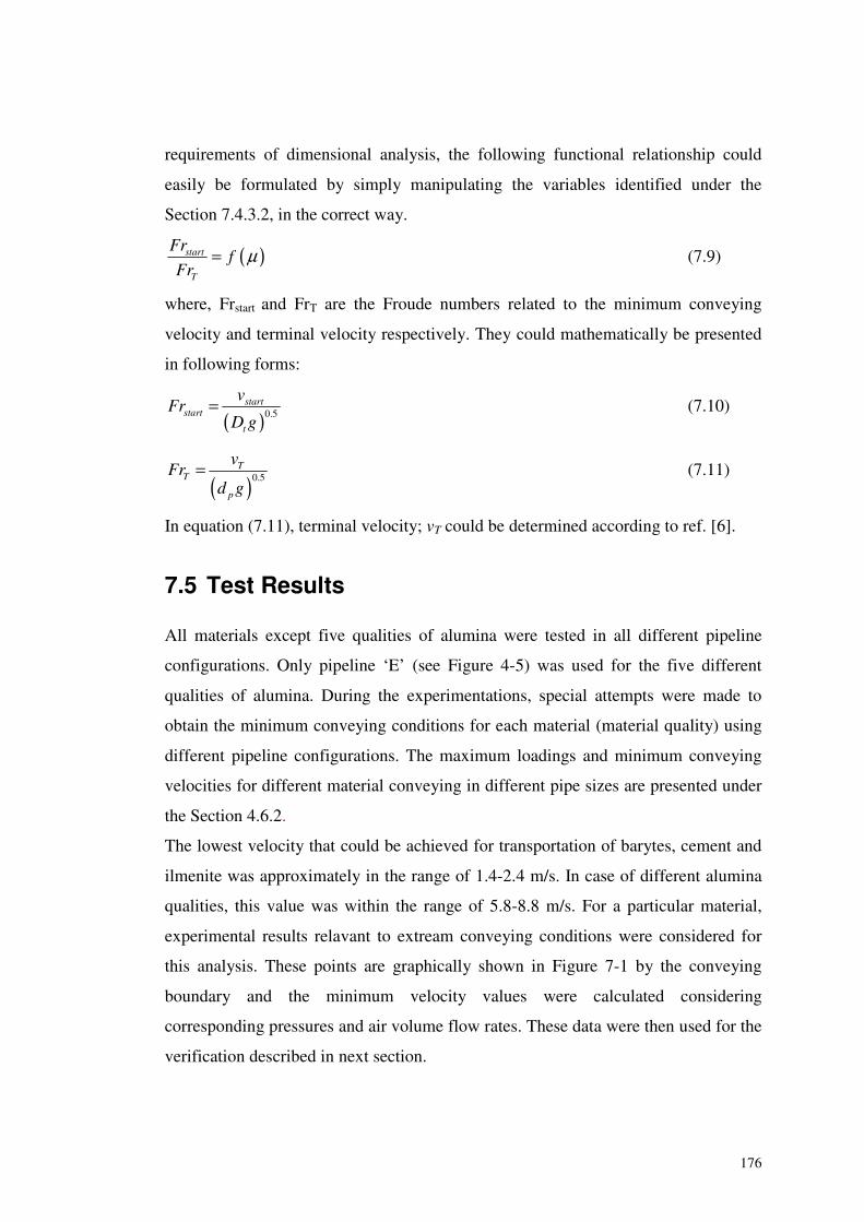
176
requirements of dimensional analysis, the following functional relationship could
easily be formulated by simply manipulating the variables identified under the
Section 7.4.3.2, in the correct way.
( )start
T
Frf
Frμ= (7.9)
where, Frstart and FrT are the Froude numbers related to the minimum conveying
velocity and terminal velocity respectively. They could mathematically be presented
in following forms:
( )0.5start
start
t
vFr
D g= (7.10)
( )0.5T
T
p
vFr
d g= (7.11)
In equation (7.11), terminal velocity; vT could be determined according to ref. [6].
7.5 Test Results
All materials except five qualities of alumina were tested in all different pipeline
configurations. Only pipeline ‘E’ (see Figure 4-5) was used for the five different
qualities of alumina. During the experimentations, special attempts were made to
obtain the minimum conveying conditions for each material (material quality) using
different pipeline configurations. The maximum loadings and minimum conveying
velocities for different material conveying in different pipe sizes are presented under
the Section 4.6.2.
The lowest velocity that could be achieved for transportation of barytes, cement and
ilmenite was approximately in the range of 1.4-2.4 m/s. In case of different alumina
qualities, this value was within the range of 5.8-8.8 m/s. For a particular material,
experimental results relavant to extream conveying conditions were considered for
this analysis. These points are graphically shown in Figure 7-1 by the conveying
boundary and the minimum velocity values were calculated considering
corresponding pressures and air volume flow rates. These data were then used for the
verification described in next section.
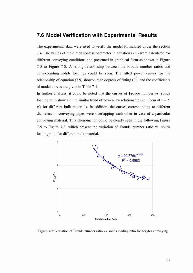
177
7.6 Model Verification with Experimental Results
The experimental data were used to verify the model formulated under the section
7.4. The values of the dimensionless parameter in equation (7.9) were calculated for
different conveying conditions and presented in graphical form as shown in Figure
7-5 to Figure 7-8. A strong relationship between the Froude number ratios and
corresponding solids loadings could be seen. The fitted power curves for the
relationship of equation (7.9) showed high degrees of fitting (R2) and the coefficients
of model curves are given in Table 7-1.
In further analysis, it could be noted that the curves of Froude number vs. solids
loading ratio show a quite similar trend of power-law relationship (i.e., form of y = C
xp) for different bulk materials. In addition, the curves corresponding to different
diameters of conveying pipes were overlapping each other in case of a particular
conveying material. This phenomenon could be clearly seen in the following Figure
7-5 to Figure 7-8, which present the variation of Froude number ratio vs. solids
loading ratio for different bulk material.
y = 90.776x-0.7032
R2 = 0.9582
0
1
2
3
0 100 200 300 400
Solids Loading Ratio
Fr s
tart/F
r T
Figure 7-5: Variation of Froude number ratio vs. solids loading ratio for barytes conveying.
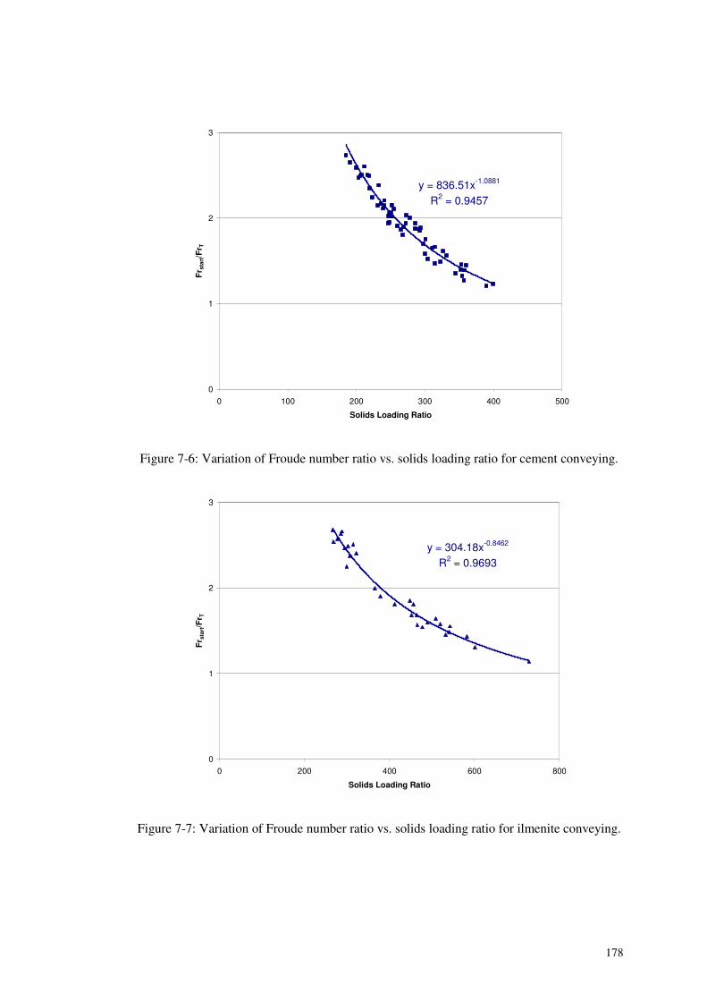
178
y = 836.51x-1.0881
R2 = 0.9457
0
1
2
3
0 100 200 300 400 500
Solids Loading Ratio
Fr s
tart/F
r T
Figure 7-6: Variation of Froude number ratio vs. solids loading ratio for cement conveying.
y = 304.18x-0.8462
R2 = 0.9693
0
1
2
3
0 200 400 600 800
Solids Loading Ratio
Fr s
tart/F
r T
Figure 7-7: Variation of Froude number ratio vs. solids loading ratio for ilmenite conveying.
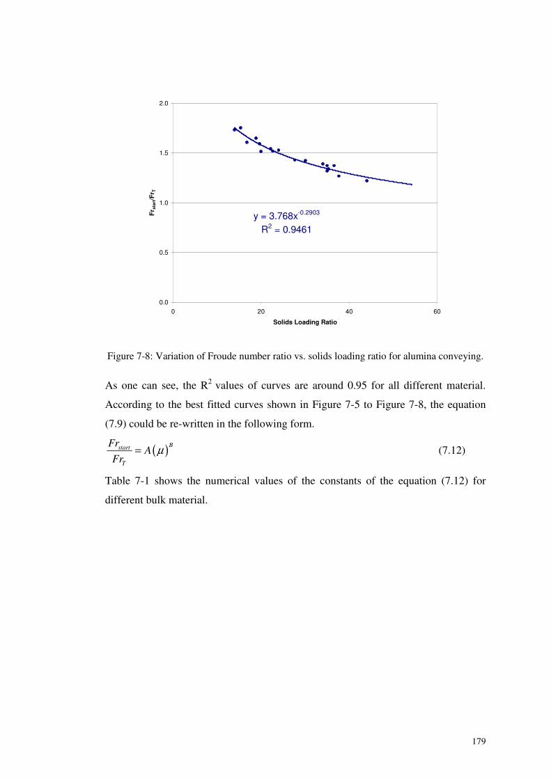
179
y = 3.768x-0.2903
R2 = 0.9461
0.0
0.5
1.0
1.5
2.0
0 20 40 60
Solids Loading Ratio
Fr s
tart/F
r T
Figure 7-8: Variation of Froude number ratio vs. solids loading ratio for alumina conveying.
As one can see, the R2 values of curves are around 0.95 for all different material.
According to the best fitted curves shown in Figure 7-5 to Figure 7-8, the equation
(7.9) could be re-written in the following form.
( )Bstart
T
FrA
Frμ= (7.12)
Table 7-1 shows the numerical values of the constants of the equation (7.12) for
different bulk material.
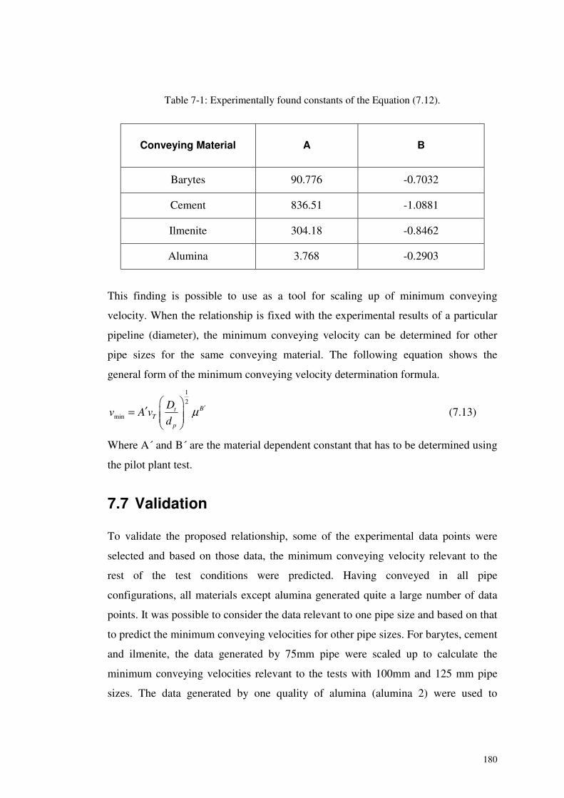
180
Table 7-1: Experimentally found constants of the Equation (7.12).
This finding is possible to use as a tool for scaling up of minimum conveying
velocity. When the relationship is fixed with the experimental results of a particular
pipeline (diameter), the minimum conveying velocity can be determined for other
pipe sizes for the same conveying material. The following equation shows the
general form of the minimum conveying velocity determination formula.
1
2
minBt
Tp
Dv A v
dμ ′
′= � �� ��
(7.13)
Where A´ and B´ are the material dependent constant that has to be determined using
the pilot plant test.
7.7 Validation
To validate the proposed relationship, some of the experimental data points were
selected and based on those data, the minimum conveying velocity relevant to the
rest of the test conditions were predicted. Having conveyed in all pipe
configurations, all materials except alumina generated quite a large number of data
points. It was possible to consider the data relevant to one pipe size and based on that
to predict the minimum conveying velocities for other pipe sizes. For barytes, cement
and ilmenite, the data generated by 75mm pipe were scaled up to calculate the
minimum conveying velocities relevant to the tests with 100mm and 125 mm pipe
sizes. The data generated by one quality of alumina (alumina 2) were used to
Conveying Material A B
Barytes 90.776 -0.7032
Cement 836.51 -1.0881
Ilmenite 304.18 -0.8462
Alumina 3.768 -0.2903
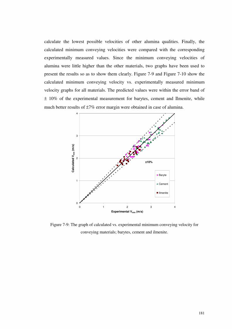
181
calculate the lowest possible velocities of other alumina qualities. Finally, the
calculated minimum conveying velocities were compared with the corresponding
experimentally measured values. Since the minimum conveying velocities of
alumina were little higher than the other materials, two graphs have been used to
present the results so as to show them clearly. Figure 7-9 and Figure 7-10 show the
calculated minimum conveying velocity vs. experimentally measured minimum
velocity graphs for all materials. The predicted values were within the error band of
± 10% of the experimental measurement for barytes, cement and Ilmenite, while
much better results of ±7% error margin were obtained in case of alumina.
0
1
2
3
4
0 1 2 3 4
Experimental Vmin (m/s)
Cal
cula
ted
Vm
in(m
/s)
Baryte
Cement
Ilmenite
±10%
Figure 7-9: The graph of calculated vs. experimental minimum conveying velocity for
conveying materials; barytes, cement and ilmenite.
182
0
4
8
12
0 4 8 12
Experimental Vmin (m/s)
Cal
cula
ted
Vm
in(m
/s)
Alumina
±7%
Figure 7-10: The graph of calculated vs. experimental minimum conveying velocity for
alumina.
7.8 Comparison with Others Models
To compare the prediction of proposed model with the other correlations described
under section 7.2, the same experimental data points were considered and the
prediction were made with the help of different correlations. The calculated values of
minimum conveying velocities were compared with the corresponding
experimentally measured values. In this cause of comparison, basically three tools
were used; worst case errors (maximum values of over-prediction and under-
prediction denoted by emax and emin respectively), standard deviations of error (σe)
and average absolute deviation of percentage error ( e ). These statistical tools are
described in details under the Section 4.8.2.2. The comparison results are shown in
Table 7-2.
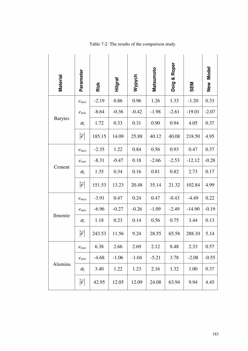
183
Table 7-2: The results of the comparison study.
Mat
eria
l
Par
amet
er
Riz
k
Hilg
raf
Wyp
ych
Mat
sum
oto
Do
ig&
Ro
per
SE
M
New
Mo
del
emax -2.19 0.86 0.96 1.26 1.33 -1.20 0.33
emin -8.64 -0.36 -0.42 -1.98 -2.61 -19.01 -2.07
σe 1.72 0.33 0.31 0.90 0.94 4.05 0.37Barytes
e 185.15 14.09 25.88 40.12 40.08 218.50 4.95
emax -2.35 1.22 0.84 0.56 0.93 0.47 0.37
emin -8.31 -0.47 0.18 -2.66 -2.53 -12.12 -0.28
σe 1.35 0.34 0.16 0.81 0.82 2.73 0.17Cement
e 151.53 13.23 20.48 35.14 21.32 102.84 4.99
emax -3.91 0.47 0.24 0.47 -0.43 -4.49 0.22
emin -6.96 -0.27 -0.26 -1.09 -2.49 -14.90 -0.19
σe 1.18 0.23 0.14 0.56 0.75 3.44 0.13Ilmenite
e 243.53 11.56 9.24 28.55 65.58 288.10 5.14
emax 6.38 2.66 2.69 2.12 8.48 2.33 0.57
emin -4.68 -1.06 -1.04 -5.21 3.78 -2.08 -0.55
σe 3.40 1.22 1.23 2.16 1.32 1.00 0.37Alumina
e 42.95 12.05 12.09 24.08 63.94 9.94 4.45
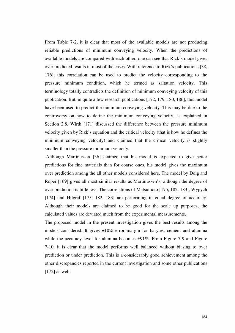
184
From Table 7-2, it is clear that most of the available models are not producing
reliable predictions of minimum conveying velocity. When the predictions of
available models are compared with each other, one can see that Rizk’s model gives
over predicted results in most of the cases. With reference to Rizk’s publications [38,
176], this correlation can be used to predict the velocity corresponding to the
pressure minimum condition, which he termed as saltation velocity. This
terminology totally contradicts the definition of minimum conveying velocity of this
publication. But, in quite a few research publications [172, 179, 180, 186], this model
have been used to predict the minimum conveying velocity. This may be due to the
controversy on how to define the minimum conveying velocity, as explained in
Section 2.8. Wirth [171] discussed the difference between the pressure minimum
velocity given by Rizk’s equation and the critical velocity (that is how he defines the
minimum conveying velocity) and claimed that the critical velocity is slightly
smaller than the pressure minimum velocity.
Although Martinussen [36] claimed that his model is expected to give better
predictions for fine materials than for coarse ones, his model gives the maximum
over prediction among the all other models considered here. The model by Doig and
Roper [169] gives all most similar results as Martinussen’s, although the degree of
over prediction is little less. The correlations of Matsumoto [175, 182, 183], Wypych
[174] and Hilgraf [175, 182, 183] are performing in equal degree of accuracy.
Although their models are claimed to be good for the scale up purposes, the
calculated values are deviated much from the experimental measurements.
The proposed model in the present investigation gives the best results among the
models considered. It gives ±10% error margin for barytes, cement and alumina
while the accuracy level for alumina becomes ±91%. From Figure 7-9 and Figure
7-10, it is clear that the model performs well balanced without biasing to over
prediction or under prediction. This is a considerably good achievement among the
other discrepancies reported in the current investigation and some other publications
[172] as well.
185
7.9 Prediction of Minimum Conveying Boundary in
Experimental PCC
Using the proposed correlation, an attempt was made to predict the minimum
conveying boundaries for different bulk materials and different pipeline
configurations. For barytes, cement and ilmenite, the data generated by 75mm pipe
were scaled up to calculate the minimum conveying boundaries relevant to the tests
with 100mm and 125 mm pipe sizes. In similar way, experimental data of alumina 2
was used to determine the minimum conveying boundaries of other alumina
qualities. The results were much compatible with the experimental measurements.
The predicted minimum conveying boundaries have been super-imposed on the
experimental pneumatic conveying characteristics of various combinations of
conveying bulk materials and pipeline configurations and few of the resulted graphs
are shown in Figure 7-11 to Figure 7-14, representing all tested materials and
different pipeline configurations used in the present investigation. The rest of the
conveying characteristic curves for other different combinations of conveying
material and pipe configuration together with their minimum conveying boundaries
determined by the proposed model are presented under Appendix B.
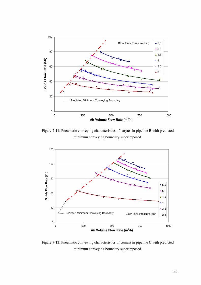
186
0
20
40
60
80
100
0 250 500 750 1000
Air Volume Flow Rate (m3/h)
So
lids
Flo
wR
ate
(t/h
)5,5
5
4.5
4
3.5
3
Blow Tank Pressure (bar)
Predicted Minimum Conveying Boundary
Figure 7-11: Pneumatic conveying characteristics of barytes in pipeline B with predicted
minimum conveying boundary superimposed.
0
40
80
120
160
200
0 250 500 750 1000
Air Volume Flow Rate (m3/h)
So
lids
Flo
wR
ate
(t/h
)
5.5
5
4.5
4
3.5
2.5Blow Tank Pressure (bar)Predicted Minimum Conveying Boundary
Figure 7-12: Pneumatic conveying characteristics of cement in pipeline C with predicted
minimum conveying boundary superimposed.
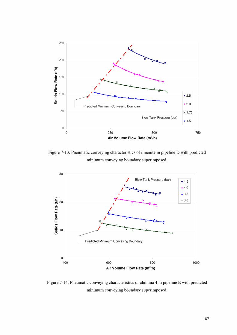
187
0
50
100
150
200
250
0 250 500 750
Air Volume Flow Rate (m3/h)
So
lids
Flo
wR
ate
(t/h
)
2.5
2.0
1.75
1.5Blow Tank Pressure (bar)
Predicted Minimum Conveying Boundary
Figure 7-13: Pneumatic conveying characteristics of ilmenite in pipeline D with predicted
minimum conveying boundary superimposed.
0
10
20
30
400 600 800 1000
Air Volume Flow Rate (m3/h)
So
lids
Flo
wR
ate
(t/h
)
4.5
4.0
3.5
3.0
Blow Tank Pressure (bar)
Predicted Minimum Conveying Boundary
Figure 7-14: Pneumatic conveying characteristics of alumina 4 in pipeline E with predicted
minimum conveying boundary superimposed.
188
One can clearly see that the minimum conveying boundary predicted by the proposed
scaling model correctly shows the experimental limit of conveying.
7.10 Conclusion
According to Figure 7-9 and Figure 7-10, it is clear that using the proposed method,
the minimum conveying velocity can be predicted with an accuracy of approximately
± 90%. This is a significant achievement amidst the large discrepancies reported
[172] in the available correlations, specially, in case of fine powders (< 100 μm). As
revealed during the comparison above, the proposed model is much superior to the
other models considered under this study. Further, since the prediction matches fairly
well with the experimental findings, this method seems to have a good potential for
use as a reliable scaling tool in pneumatic conveying system designs, especially
conjunction with the proposed scaling up technique under the Section 4.
189
8 PUTTING IT ALL TOGETHER AND A CASESTUDY
The scaling up model of line pressure drop and line entry pressure loss were
combined together with the scaling up model of minimum conveying velocity to
form a complete scaling up technique for pneumatic conveying system. With the aim
of using them in designing of industrial scale pneumatic conveying systems, all these
models were put together with the help of a computer programme to form a general
calculation programme. The following sections are describing the structure of the
software programme, calculation procedure adopted, etc, in detail. At the end of the
chapter, the results of an investigation where the newly formulated calculation
programme was used to determine the pressure drop and velocity of an industrial
scale pneumatic conveying plant are given in a form of a case study.
8.1 Introduction
Since the calculation procedure consists of some sort of repetitive calculations, it was
decided to set-up a computer based calculation programme that can be used as
general software in pneumatic conveying system designs. As an initial step,
Microsoft Excel® was used to formulate the general calculation programme.
The basic necessity of the calculation programme is that the results of preliminary
conveying tests conducted in a laboratory scale pilot plant, are available for the
conveying bulk material and all the relationships relevant to different scaling models
proposed under the current investigation are known for at least one pipe diameter.
The calculation software is programmed so that it easily calculates the pressure drop
across each and individual pipe sections. In addition, the conveying velocity is also
calculated.
To check the validity of the software programme, it was used in a design procedure
of an industrial scale conveying system. The comparison of calculated and
experimental results is presented at the end of the chapter.

190
8.2 General Calculation Programme
This calculation programme basically consists of four main sections;
1. Implementation of the model relationships formulated from the pilot plant
tests for different pipe elements.
2. Introduction of design inputs together with provisional parameters
3. Pressure drop and velocity calculations
4. Presentation of output results
Each of the above stages is briefly described in following sections.
8.2.1 Implementation of Model Relationships
According to the conclusions made in relevant sections, it was clear that the
relationships derived in Chapters 4, 6 and 7, were independent of conveying pipe
sizes and the predictions could be made for different pipe sizes by just conducting a
series of tests with conveying bulk material in one particular pipe diameter.
Consequently, the calculation programme is based on the findings of the pilot plant
tests and the experimentally found functional relationships of different parameters
for individual pipe elements, as mentioned earlier. In cases of entry pressure loss and
minimum conveying velocity, the numerical values of the functional relationships
that are shown in equations (6.21) and (7.9) could be used in the calculation
programme. In case of the scaling model for line pressure drop described in Chapter
4, the numerical constants of the functional relationship between the K and V2entry
have to be introduced. In addition, the asymptotic constant value of K for high entry
velocity values (see Figure 4-15 to Figure 4-20) and corresponding lowest velocities
have to be used in the calculation programme.
All those parameters in numerical form are put in one sheet and it is named as ‘Pilot
Plant Test Results’. One screen shot of it is shown in Figure 8-1.
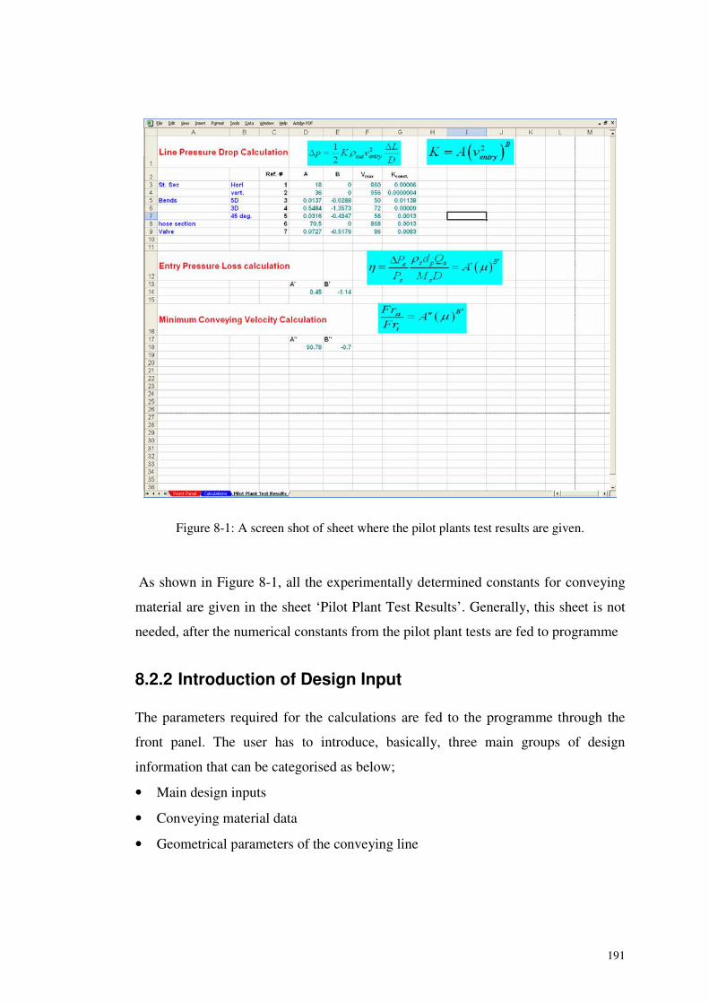
191
Figure 8-1: A screen shot of sheet where the pilot plants test results are given.
As shown in Figure 8-1, all the experimentally determined constants for conveying
material are given in the sheet ‘Pilot Plant Test Results’. Generally, this sheet is not
needed, after the numerical constants from the pilot plant tests are fed to programme
8.2.2 Introduction of Design Input
The parameters required for the calculations are fed to the programme through the
front panel. The user has to introduce, basically, three main groups of design
information that can be categorised as below;
• Main design inputs
• Conveying material data
• Geometrical parameters of the conveying line
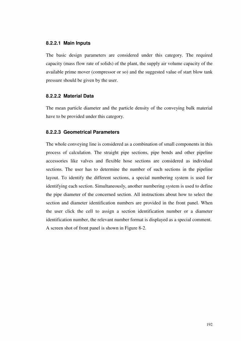
192
8.2.2.1 Main Inputs
The basic design parameters are considered under this category. The required
capacity (mass flow rate of solids) of the plant, the supply air volume capacity of the
available prime mover (compressor or so) and the suggested value of start blow tank
pressure should be given by the user.
8.2.2.2 Material Data
The mean particle diameter and the particle density of the conveying bulk material
have to be provided under this category.
8.2.2.3 Geometrical Parameters
The whole conveying line is considered as a combination of small components in this
process of calculation. The straight pipe sections, pipe bends and other pipeline
accessories like valves and flexible hose sections are considered as individual
sections. The user has to determine the number of such sections in the pipeline
layout. To identify the different sections, a special numbering system is used for
identifying each section. Simultaneously, another numbering system is used to define
the pipe diameter of the concerned section. All instructions about how to select the
section and diameter identification numbers are provided in the front panel. When
the user click the cell to assign a section identification number or a diameter
identification number, the relevant number format is displayed as a special comment.
A screen shot of front panel is shown in Figure 8-2.
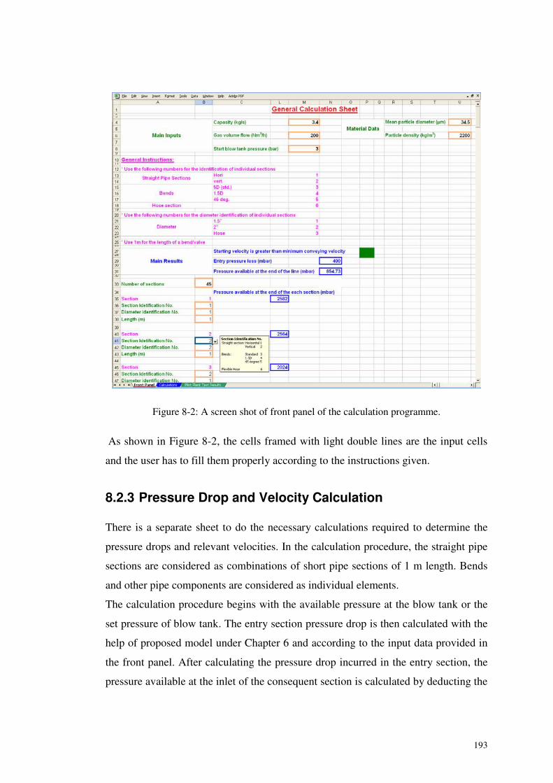
193
Figure 8-2: A screen shot of front panel of the calculation programme.
As shown in Figure 8-2, the cells framed with light double lines are the input cells
and the user has to fill them properly according to the instructions given.
8.2.3 Pressure Drop and Velocity Calculation
There is a separate sheet to do the necessary calculations required to determine the
pressure drops and relevant velocities. In the calculation procedure, the straight pipe
sections are considered as combinations of short pipe sections of 1 m length. Bends
and other pipe components are considered as individual elements.
The calculation procedure begins with the available pressure at the blow tank or the
set pressure of blow tank. The entry section pressure drop is then calculated with the
help of proposed model under Chapter 6 and according to the input data provided in
the front panel. After calculating the pressure drop incurred in the entry section, the
pressure available at the inlet of the consequent section is calculated by deducting the
194
entry loss from the available pressure in the blow tank. In next sections, pertinent
pressure drops for each pipe sections are calculated according to the models
proposed under Chapter 4. A kind of cell reference technique is used to take the
appropriate data from front panel and required model constants from ‘Pilot Plant Test
Results’ sheet. In the calculation process, the pressure values are updated after each
and every pipe sections and the same calculation procedure continues until the end of
the line.
In addition to the above described pressure drop calculation, the minimum conveying
velocity is calculated with the help of the model proposed in Chapter 7, using the
material constants given in ‘Pilot Plant Test Results’ sheet. The velocity at the
starting point of the conveying line can also be calculated using the given inputs in
front panel. These two velocity values are compared and result is shown in front
panel.
Usually the calculation sheet is also kept hidden, since the user has no need
interaction there.
8.2.4 Presentation of Output Results
The entry pressure loss together with the pressure drop values encountered in each
and every section is presented as results. Also, the pressure available at the end of the
conveying line is given. In addition, the indication is given by comparing the
calculated start velocity at the entry section and the scaled up minimum conveying
velocity from the pilot plant test. When the start velocity is lower than the minimum
conveying velocity, the phrase ‘Starting velocity is less than the minimum conveying
velocity’ is appeared with a red blinking. Otherwise, the phrase ‘Starting velocity is
greater than minimum conveying velocity’ will be displayed with green button.
For the ease of presentation, the output results are also shown in front panel. This can
be clearly seen in Figure 8-2. The results are shown in cells framed with thick lines.
195
8.3 Use of Calculation Programme
Once the pneumatic conveying tests are concluded in a laboratory scale pilot plant at
least with one pipe size, the required relationships among the interesting parameters
can be established easily for the particular bulk material. On the other hand, the
relationships and models formulated during the present investigation have been
proven to be valid for both dilute and dense phase conveying modes. Consequently,
the both of these conveying modes can be dealt with the calculation programme
without any trouble.
The advantage of the calculation program is that once the relevant parameters are
fed, it can be used to predict the performance of different pipeline configurations
together with different combinations of design inputs such as plant capacity, blow
tank pressure values, etc. This kind of trials can be easily performed by just changing
one or more of the considered parameters and checking the cell output called
‘Pressure available at the end of the line’. If the value is negative, it means the assign
values are not suitable for the particular pipeline configuration. Otherwise, the user
can optimise the design inputs so that the pressure available at the end of the line is
minimised.
Simultaneously, the user has to check the status of the conveying velocity at the
starting point of the pipeline. As mentioned under section 8.2.4, the displayed phrase
is changing automatically according to the comparison status of the start velocity
with the minimum conveying velocity for the particular material and pipe
configuration. This can also be recognised without any trouble by the colour status of
the indication cell just beside the main results.
Since the input parameters and output results are displayed in a common sheet, the
above mentioned trial procedure can easily be performed. If the user is concerned
about the available pressures at particular point or points on the conveying line, the
relevant section has to be checked by scrolling down in the front panel.
In addition to the above explained tasks, this calculation programme can
straightforwardly be used to obtain the pneumatic conveying characteristics of the
considered bulk material in the considered pipeline configuration, by just changing
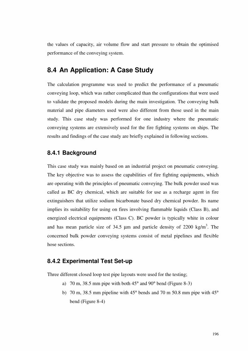
196
the values of capacity, air volume flow and start pressure to obtain the optimised
performance of the conveying system.
8.4 An Application: A Case Study
The calculation programme was used to predict the performance of a pneumatic
conveying loop, which was rather complicated than the configurations that were used
to validate the proposed models during the main investigation. The conveying bulk
material and pipe diameters used were also different from those used in the main
study. This case study was performed for one industry where the pneumatic
conveying systems are extensively used for the fire fighting systems on ships. The
results and findings of the case study are briefly explained in following sections.
8.4.1 Background
This case study was mainly based on an industrial project on pneumatic conveying.
The key objective was to assess the capabilities of fire fighting equipments, which
are operating with the principles of pneumatic conveying. The bulk powder used was
called as BC dry chemical, which are suitable for use as a recharge agent in fire
extinguishers that utilize sodium bicarbonate based dry chemical powder. Its name
implies its suitability for using on fires involving flammable liquids (Class B), and
energized electrical equipments (Class C). BC powder is typically white in colour
and has mean particle size of 34.5 μm and particle density of 2200 kg/m3. The
concerned bulk powder conveying systems consist of metal pipelines and flexible
hose sections.
8.4.2 Experimental Test Set-up
Three different closed loop test pipe layouts were used for the testing;
a) 70 m, 38.5 mm pipe with both 45° and 90° bend (Figure 8-3)
b) 70 m, 38.5 mm pipeline with 45° bends and 70 m 50.8 mm pipe with 45°
bend (Figure 8-4)
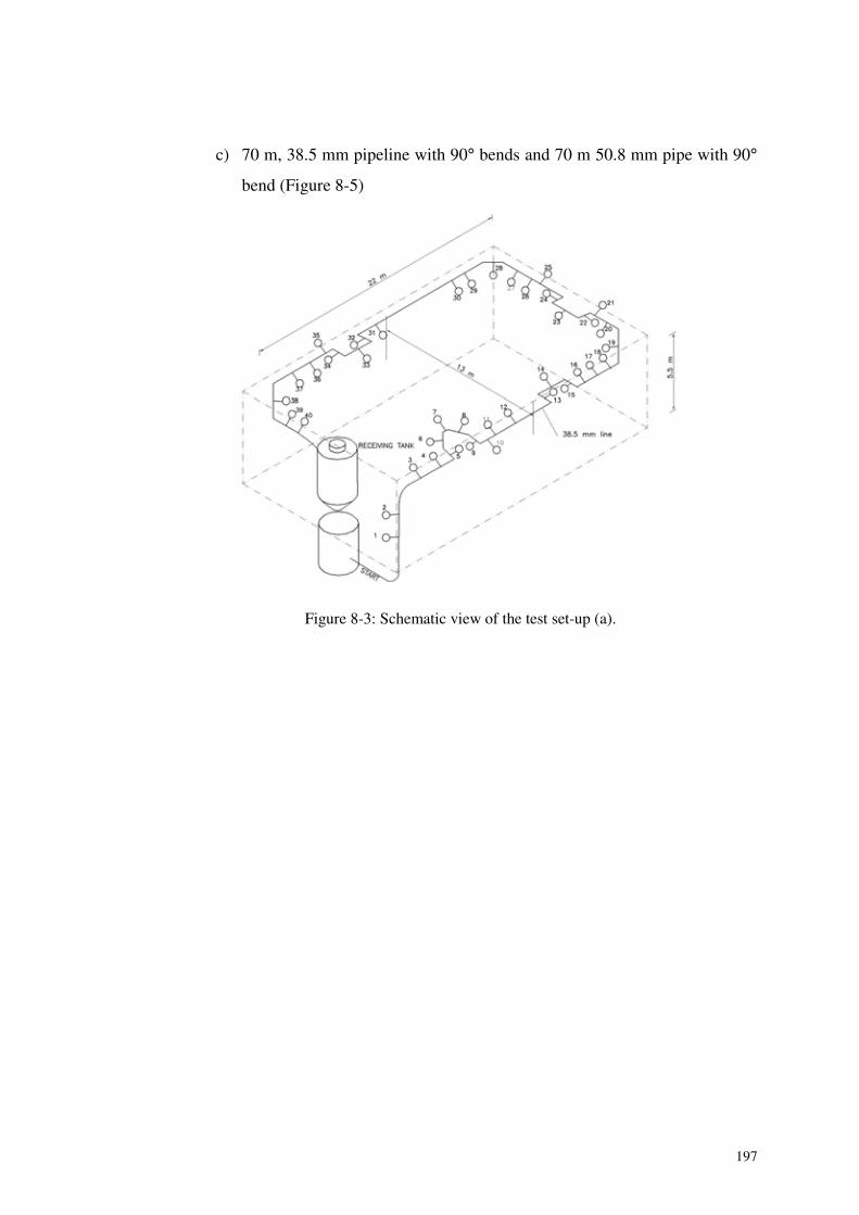
197
c) 70 m, 38.5 mm pipeline with 90° bends and 70 m 50.8 mm pipe with 90°
bend (Figure 8-5)
Figure 8-3: Schematic view of the test set-up (a).
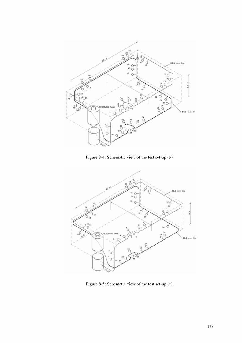
198
Figure 8-4: Schematic view of the test set-up (b).
Figure 8-5: Schematic view of the test set-up (c).
199
A large number of pressure transducers were located on the pipeline so as to isolate
the pressure drop components of each concerned sections. In case of bends, two
pressure transducers were fixed before and after each bend. Similarly, two pressure
transducers were used for each straight (both vertical and horizontal) pipe sections
with an approximate distance of 2 m, as explained in Chapter 4.
8.4.3 Usage of the Calculation Programme
The set up shown in Figure 8-3 (test set-up (a)) was selected as the base for the
calculation programme (i.e., it was considered as the pilot plant), since it consisted of
all types of bends that were used in other pipeline configurations. The K vs. v2entry
curves generated from the data relevant to the said set-up was fed to the calculation
programme. Then, the calculation programme was used to predict the performances
of the other pipeline configurations. The pressure values calculated using the
calculation programme were compared with corresponding experimental
measurements at the different points on the pipe layouts. The comparison curves
correspond to test set-ups (b) and (c) are shown in Figure 8-6 and Figure 8-7
respectively. The different curves were plotted for different release pressure (blow
tank set pressure) values.
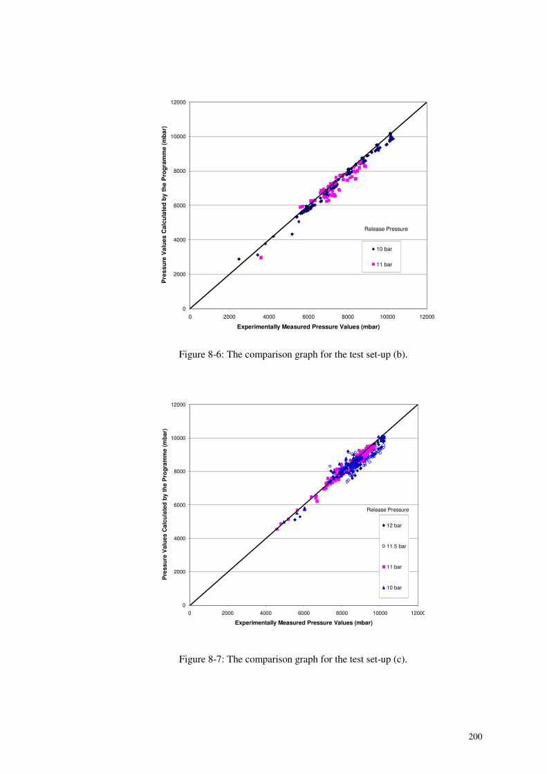
200
0
2000
4000
6000
8000
10000
12000
0 2000 4000 6000 8000 10000 12000
Experimentally Measured Pressure Values (mbar)
Pre
ssu
reV
alu
esC
alcu
late
db
yth
eP
rog
ram
me
(mb
ar)
10 bar
11 bar
Release Pressure
Figure 8-6: The comparison graph for the test set-up (b).
0
2000
4000
6000
8000
10000
12000
0 2000 4000 6000 8000 10000 12000
Experimentally Measured Pressure Values (mbar)
Pre
ssu
reV
alu
esC
alcu
late
db
yth
eP
rog
ram
me
(mb
ar)
12 bar
11.5 bar
11 bar
10 bar
Release Pressure
Figure 8-7: The comparison graph for the test set-up (c).
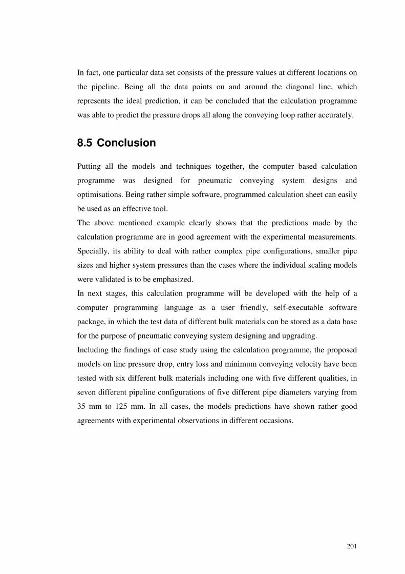
201
In fact, one particular data set consists of the pressure values at different locations on
the pipeline. Being all the data points on and around the diagonal line, which
represents the ideal prediction, it can be concluded that the calculation programme
was able to predict the pressure drops all along the conveying loop rather accurately.
8.5 Conclusion
Putting all the models and techniques together, the computer based calculation
programme was designed for pneumatic conveying system designs and
optimisations. Being rather simple software, programmed calculation sheet can easily
be used as an effective tool.
The above mentioned example clearly shows that the predictions made by the
calculation programme are in good agreement with the experimental measurements.
Specially, its ability to deal with rather complex pipe configurations, smaller pipe
sizes and higher system pressures than the cases where the individual scaling models
were validated is to be emphasized.
In next stages, this calculation programme will be developed with the help of a
computer programming language as a user friendly, self-executable software
package, in which the test data of different bulk materials can be stored as a data base
for the purpose of pneumatic conveying system designing and upgrading.
Including the findings of case study using the calculation programme, the proposed
models on line pressure drop, entry loss and minimum conveying velocity have been
tested with six different bulk materials including one with five different qualities, in
seven different pipeline configurations of five different pipe diameters varying from
35 mm to 125 mm. In all cases, the models predictions have shown rather good
agreements with experimental observations in different occasions.
202
9 COMPUTATIONAL FLUID DYNAMICS AS APRESSURE DROP PREDICTION TOOL INDENSE PHASE PNEUMATIC CONVEYINGSYSTEMS
9.1 Introduction
As an alternative approach to the classical methods of analysing gas-solid flows,
computational techniques have been a well-accepted tool, throughout the last two
decades. Specially, Computational Fluid Dynamics (CFD) technique, which means a
computational technology that enables one to study the dynamics of single and multi-
phase flows, has been becoming popular in scientific research field and industry of
two-phase flow systems. In fact, CFD is increasingly used in all branches of
engineering. Originally applied to aerodynamic problems in the aerospace industry,
with advances in computer processing power and more powerful numerical methods,
it can now be applied to more complex situations. With the invention of high- speed
high-capacity desk top personal computers, scientists and researches have
extensively been using several large scale commercial computer codes to predict the
flow phenomena in pneumatic conveying systems, which are very complicate to deal
with only first principle based prediction methods.
As discussed under Section 2.11.2, although a number of numerical simulations have
been carried out to model the flow phenomena of pneumatic conveying systems,
those relevant to dense phase systems could rarely be seen among them. On the other
hand, only few attempts could be found where the CFD techniques have been used to
predict the line pressure drop of a pneumatic conveying system.
As a part of the present research, a CFD simulation was included to investigate the
pressure drop prediction capabilities of CFD techniques in the dense phase flow
conditions of a pneumatic conveying system. The main objective of this work was to
investigate how good the predictions of a commercial CFD code when it is compared
with the experimental observations of a dense phase pneumatic conveying system.
203
Rather than developing a research purpose code to carry out two-phase flow
simulations from the very beginning, it might be more advantageous to use
commercially distributed and widely spread software. A well-known CFD software
code; Fluent® was used for the simulation and basically, two major parts of a
conveying line were addressed; a short straight pipe section and a standard 90° bend.
With a numerous number of experimental data generated by different conveying
materials and pipeline configurations, it could be possible to compare the simulation
results with the real experimental measurements with respect to different
combinations of those. The determination of pressure drop across the considered pipe
sections was the main focal point, while few other parameters like variation of solid
volume fraction, variation of velocity profiles, etc, were also investigated.
9.2 Background
In Section 2.11, the applications of CFD in gas-solid flow systems were briefly
discussed together with their historical evolutions. The following paragraphs will
give a brief summery of the current status of CFD applications in pneumatic
conveying.
Among the two basic approaches of CFD; Eulerian and Lagrangian approaches, the
Lagrangian method has been found to be more suited for dilute flows, since it has
limited applicability to dense flows because it may be necessary to include an
enormous number of particles. On the other hand, the Euler-Euler granular model is
suitable for dense gas-solids flows. Some investigations, which tried to predict the
gas-solid system behaviours using Eulerian approach, came with interesting results
[113, 130, 187, 188].
In recent years, a break through could be achieved, specially in the CFD applications
of dense phase gas-solid flow systems when some research works [189-193]
discussed the dynamics of inter-particle collisions. Based on this concept, Gidaspow
[194] explained the kinetic theory approach, which uses one equation model to
determine the turbulent kinetic energy of the particles in terms of the granular
temperature.
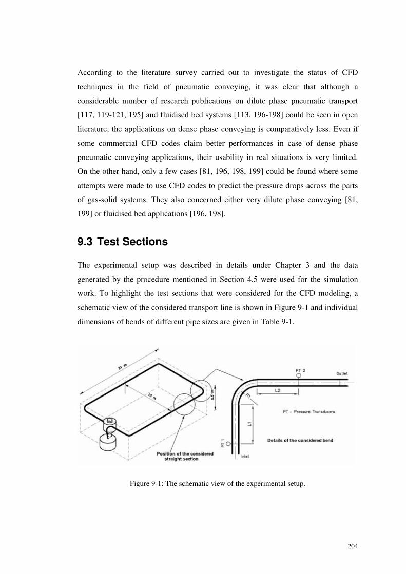
204
According to the literature survey carried out to investigate the status of CFD
techniques in the field of pneumatic conveying, it was clear that although a
considerable number of research publications on dilute phase pneumatic transport
[117, 119-121, 195] and fluidised bed systems [113, 196-198] could be seen in open
literature, the applications on dense phase conveying is comparatively less. Even if
some commercial CFD codes claim better performances in case of dense phase
pneumatic conveying applications, their usability in real situations is very limited.
On the other hand, only a few cases [81, 196, 198, 199] could be found where some
attempts were made to use CFD codes to predict the pressure drops across the parts
of gas-solid systems. They also concerned either very dilute phase conveying [81,
199] or fluidised bed applications [196, 198].
9.3 Test Sections
The experimental setup was described in details under Chapter 3 and the data
generated by the procedure mentioned in Section 4.5 were used for the simulation
work. To highlight the test sections that were considered for the CFD modeling, a
schematic view of the considered transport line is shown in Figure 9-1 and individual
dimensions of bends of different pipe sizes are given in Table 9-1.
Figure 9-1: The schematic view of the experimental setup.
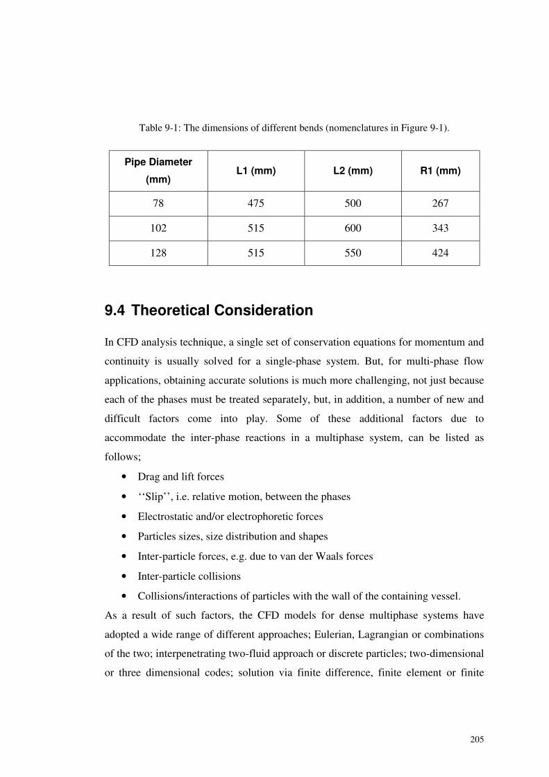
205
Table 9-1: The dimensions of different bends (nomenclatures in Figure 9-1).
Pipe Diameter
(mm)L1 (mm) L2 (mm) R1 (mm)
78 475 500 267
102 515 600 343
128 515 550 424
9.4 Theoretical Consideration
In CFD analysis technique, a single set of conservation equations for momentum and
continuity is usually solved for a single-phase system. But, for multi-phase flow
applications, obtaining accurate solutions is much more challenging, not just because
each of the phases must be treated separately, but, in addition, a number of new and
difficult factors come into play. Some of these additional factors due to
accommodate the inter-phase reactions in a multiphase system, can be listed as
follows;
• Drag and lift forces
• ‘‘Slip’’, i.e. relative motion, between the phases
• Electrostatic and/or electrophoretic forces
• Particles sizes, size distribution and shapes
• Inter-particle forces, e.g. due to van der Waals forces
• Inter-particle collisions
• Collisions/interactions of particles with the wall of the containing vessel.
As a result of such factors, the CFD models for dense multiphase systems have
adopted a wide range of different approaches; Eulerian, Lagrangian or combinations
of the two; interpenetrating two-fluid approach or discrete particles; two-dimensional
or three dimensional codes; solution via finite difference, finite element or finite
206
volume approaches, etc. In the process of introducing additional sets of conservation
equations, the original set must also be modified. The introduction of the volume
fractions of gas and solid phases and the exchange mechanism for the momentum
between the phases are the main modifications for a multi-phase CFD model.
9.4.1 CFD Model
As mentioned earlier, Fluent® (version 6.1) was used to simulate the flow across the
considered sections. The Euler-Euler granular multiphase model, which considers the
solid and gas phases as interpenetrating continuum that share the space, has been
used for this simulation. Generally, Fluent® uses a control-volume based technique to
convert the governing differential equations of the flow system to algebraic
equations, which can be solved numerically. The volume averaged dicretization
approach consists of integrating the governing equations about each and every
control volume, generating separate equations that conserve each quality on a
control-volume basis. The discretized equations, along with the initial and boundary
conditions, were solved to obtain a numerical solution. Conservation equations of
mass and momentum were developed using the Eulerian approach, and solved
simultaneously by considering the phases separately but linking them through the
drag forces in the momentum equation. In the Fluent® software code, the Phase
Coupled SIMPLE (PC-SIMPLE) algorithm that is an extension of the SIMPLE
algorithm [111] to multiphase flows is used for the pressure-velocity coupling. The
velocities are solved coupled by phases, but in a segregated fashion. A pressure
correction equation is built based on total volume continuity rather than mass
continuity. Pressure and velocities are then corrected so as to satisfy the continuity
constraint. To model the turbulence, the k-� (k: turbulent kinetic energy, �: turbulent
kinetic energy dissipation) model has been used.
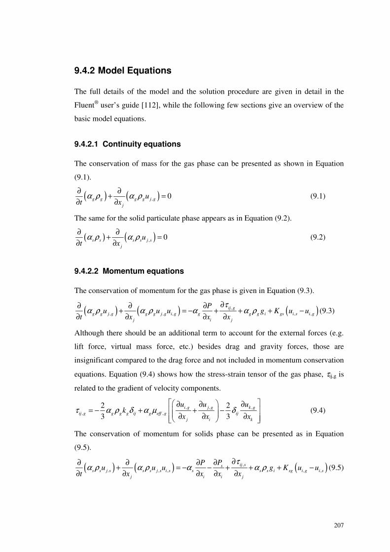
207
9.4.2 Model Equations
The full details of the model and the solution procedure are given in detail in the
Fluent® user’s guide [112], while the following few sections give an overview of the
basic model equations.
9.4.2.1 Continuity equations
The conservation of mass for the gas phase can be presented as shown in Equation
(9.1).
( ) ( ), 0g g g g j gj
ut xα ρ α ρ∂ ∂+ =
∂ ∂(9.1)
The same for the solid particulate phase appears as in Equation (9.2).
( ) ( ), 0s s s s j sj
ut xα ρ α ρ∂ ∂+ =
∂ ∂(9.2)
9.4.2.2 Momentum equations
The conservation of momentum for the gas phase is given in Equation (9.3).
( ) ( ) ( ),, , , , ,
ij gg g j g g g j g i g g g g i gs i s i g
j i j
Pu u u g K u u
t x x x
τα ρ α ρ α α ρ
∂∂ ∂ ∂+ = − + + + −∂ ∂ ∂ ∂
(9.3)
Although there should be an additional term to account for the external forces (e.g.
lift force, virtual mass force, etc.) besides drag and gravity forces, those are
insignificant compared to the drag force and not included in momentum conservation
equations. Equation (9.4) shows how the stress-strain tensor of the gas phase, τij,g is
related to the gradient of velocity components.
, , ,, ,
2 2
3 3i g j g k g
ij g g g g ij g eff g ijj i k
u u uk
x x xτ α ρ δ α μ δ
� � ∂ ∂ ∂= − + + −� �� �� �∂ ∂ ∂� �� � �
(9.4)
The conservation of momentum for solids phase can be presented as in Equation
(9.5).
( ) ( ) ( ),. , , , ,
ij sss s j s s s j s i s s s s i sg i g i s
j i i j
PPu u u g K u u
t x x x x
τα ρ α ρ α α ρ
∂∂∂ ∂ ∂+ = − − + + + −∂ ∂ ∂ ∂ ∂
(9.5)
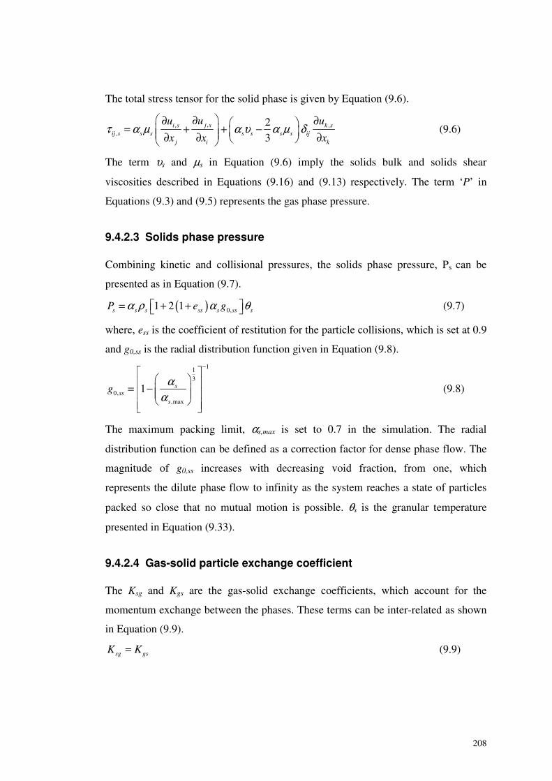
208
The total stress tensor for the solid phase is given by Equation (9.6).
,, ,,
2
3j si s k s
ij s s s s s s s ijj i k
uu u
x x xτ α μ α υ α μ δ
∂∂ ∂ = + + −� � � �� �∂ ∂ ∂� � (9.6)
The term υs and μs in Equation (9.6) imply the solids bulk and solids shear
viscosities described in Equations (9.16) and (9.13) respectively. The term ‘P’ in
Equations (9.3) and (9.5) represents the gas phase pressure.
9.4.2.3 Solids phase pressure
Combining kinetic and collisional pressures, the solids phase pressure, Ps can be
presented as in Equation (9.7).
( ) 0,1 2 1s s s ss s ss sP e gα ρ α θ� �= + +� � (9.7)
where, ess is the coefficient of restitution for the particle collisions, which is set at 0.9
and g0,ss is the radial distribution function given in Equation (9.8).
11
3
0,,max
1 sss
s
gαα
−� �
� �= − � �� �� �� � �� �
(9.8)
The maximum packing limit, αs,max is set to 0.7 in the simulation. The radial
distribution function can be defined as a correction factor for dense phase flow. The
magnitude of g0,ss increases with decreasing void fraction, from one, which
represents the dilute phase flow to infinity as the system reaches a state of particles
packed so close that no mutual motion is possible. θs is the granular temperature
presented in Equation (9.33).
9.4.2.4 Gas-solid particle exchange coefficient
The Ksg and Kgs are the gas-solid exchange coefficients, which account for the
momentum exchange between the phases. These terms can be inter-related as shown
in Equation (9.9).
sg gsK K= (9.9)
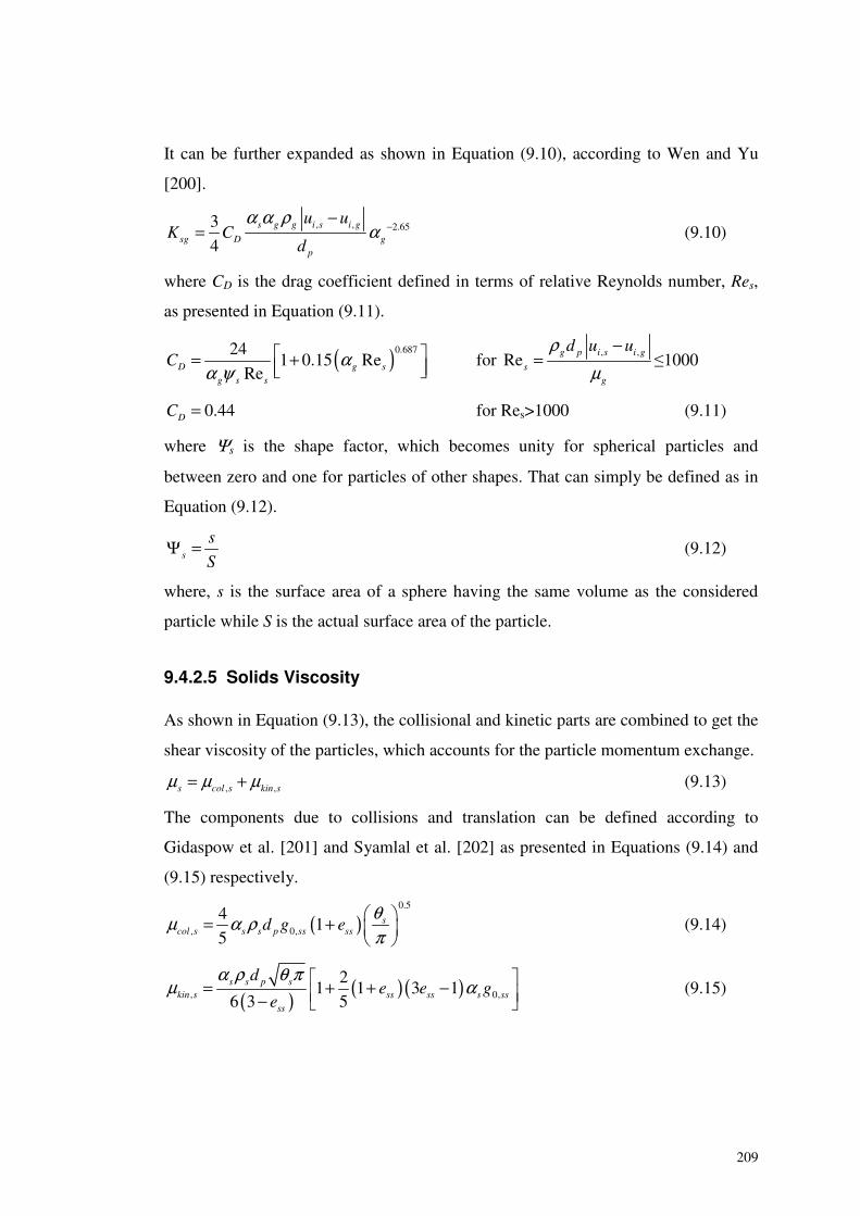
209
It can be further expanded as shown in Equation (9.10), according to Wen and Yu
[200].
, , 2.653
4s g g i s i g
sg D gp
u uK C
d
α α ρα −
−= (9.10)
where CD is the drag coefficient defined in terms of relative Reynolds number, Res,
as presented in Equation (9.11).
( )0.687241 0.15 Re
ReD g sg s s
C αα ψ
� �= +� �� �for
, ,Re
g p i s i g
sg
d u uρμ−
= �1000
0.44DC = for Res>1000 (9.11)
where Ψs is the shape factor, which becomes unity for spherical particles and
between zero and one for particles of other shapes. That can simply be defined as in
Equation (9.12).
s
s
SΨ = (9.12)
where, s is the surface area of a sphere having the same volume as the considered
particle while S is the actual surface area of the particle.
9.4.2.5 Solids Viscosity
As shown in Equation (9.13), the collisional and kinetic parts are combined to get the
shear viscosity of the particles, which accounts for the particle momentum exchange.
, ,s col s kin sμ μ μ= + (9.13)
The components due to collisions and translation can be defined according to
Gidaspow et al. [201] and Syamlal et al. [202] as presented in Equations (9.14) and
(9.15) respectively.
( )0.5
, 0,
41
5s
col s s s p ss ssd g eθμ α ρπ
= + � ��
(9.14)
( ) ( )( ), 0,
21 1 3 1
6 3 5s s p s
kin s ss ss s ssss
de e g
e
α ρ θ πμ α� �= + + −� �− � �
(9.15)
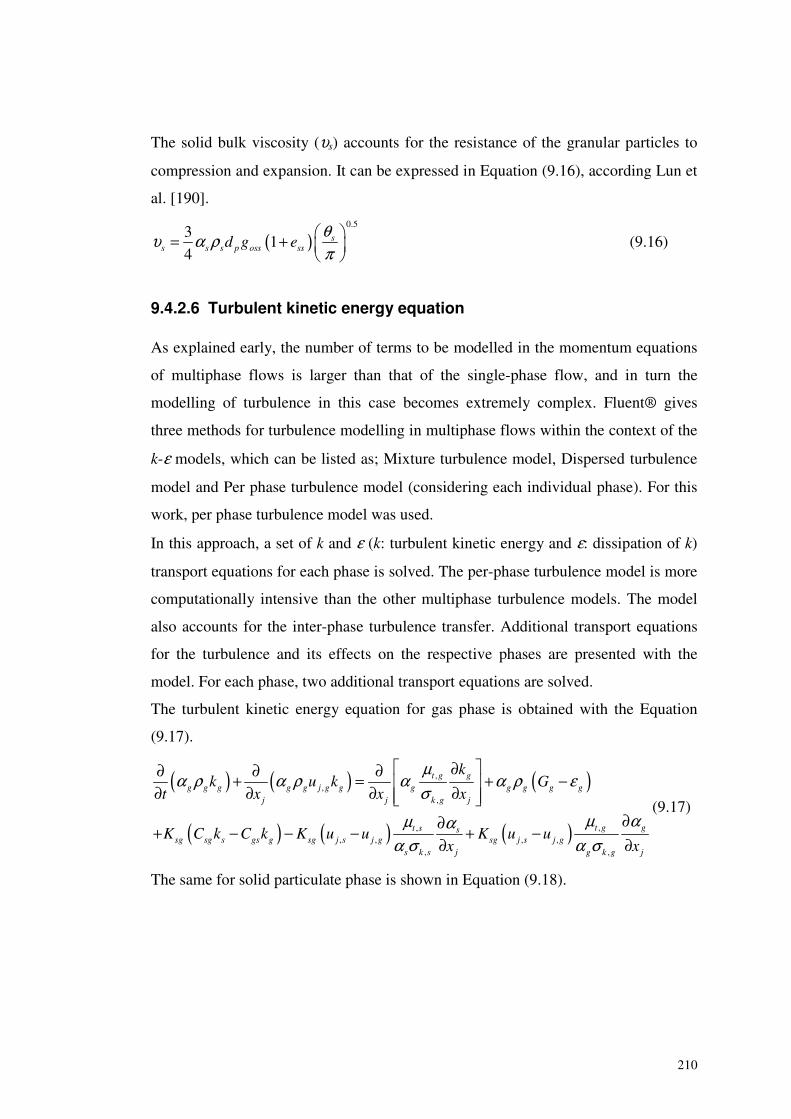
210
The solid bulk viscosity (υs) accounts for the resistance of the granular particles to
compression and expansion. It can be expressed in Equation (9.16), according Lun et
al. [190].
( )0.5
31
4s
s s s p oss ssd g eθυ α ρπ
= + � ��
(9.16)
9.4.2.6 Turbulent kinetic energy equation
As explained early, the number of terms to be modelled in the momentum equations
of multiphase flows is larger than that of the single-phase flow, and in turn the
modelling of turbulence in this case becomes extremely complex. Fluent® gives
three methods for turbulence modelling in multiphase flows within the context of the
k-ε models, which can be listed as; Mixture turbulence model, Dispersed turbulence
model and Per phase turbulence model (considering each individual phase). For this
work, per phase turbulence model was used.
In this approach, a set of k and ε (k: turbulent kinetic energy and ε: dissipation of k)
transport equations for each phase is solved. The per-phase turbulence model is more
computationally intensive than the other multiphase turbulence models. The model
also accounts for the inter-phase turbulence transfer. Additional transport equations
for the turbulence and its effects on the respective phases are presented with the
model. For each phase, two additional transport equations are solved.
The turbulent kinetic energy equation for gas phase is obtained with the Equation
(9.17).
( ) ( ) ( )
( ) ( ) ( )
,,
,
,,, , , ,
, ,
t g gg g g g g j g g g g g g g
j j k g j
t g gt s ssg sg s gs g sg j s j g sg j s j g
s k s j g k g j
kk u k G
t x x x
K C k C k K u u K u ux x
μα ρ α ρ α α ρ ε
σ
μ αμ αα σ α σ
� �∂∂ ∂ ∂+ = + −� �∂ ∂ ∂ ∂� �� �∂∂+ − − − + −
∂ ∂
(9.17)
The same for solid particulate phase is shown in Equation (9.18).
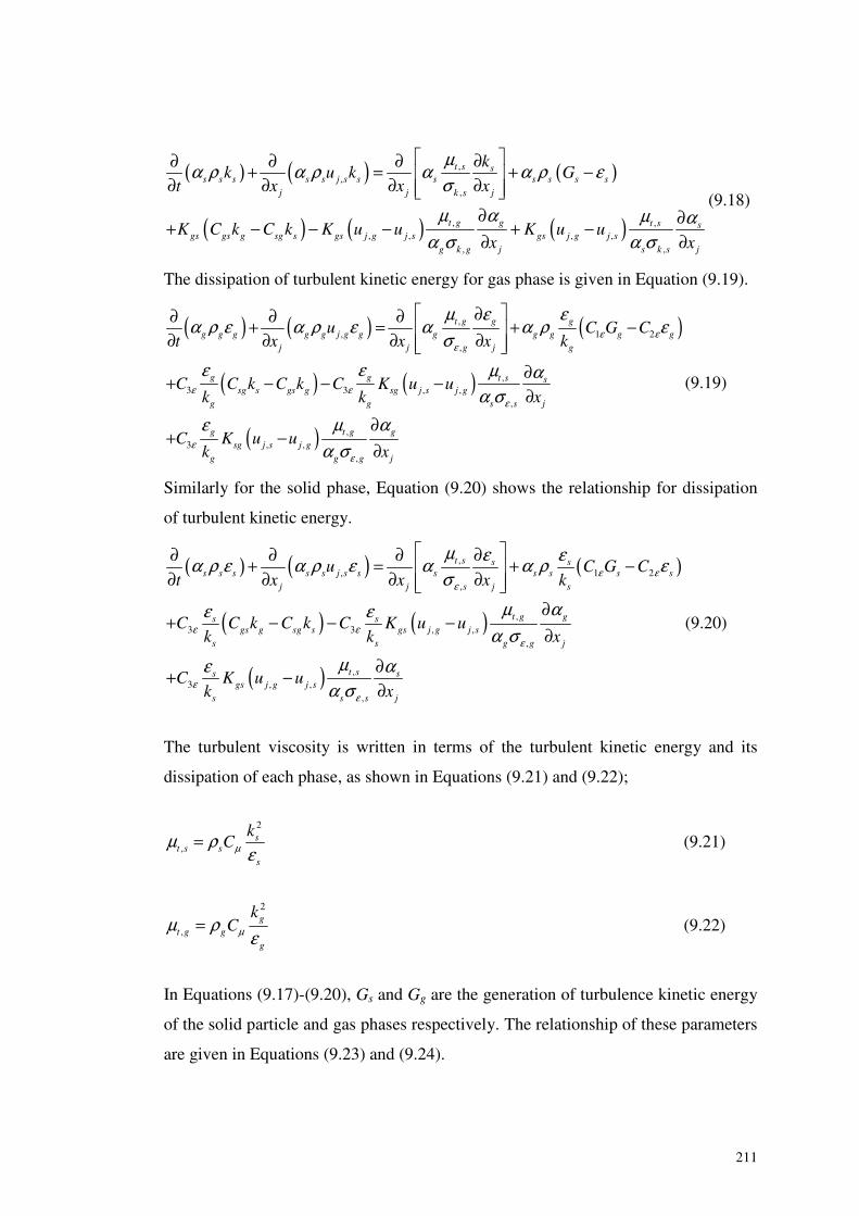
211
( ) ( ) ( )
( ) ( ) ( )
,,
,
, ,, , , ,
, ,
t s ss s s s s j s s s s s s s
j j k s j
t g g t s sgs gs g sg s gs j g j s gs j g j s
g k g j s k s j
kk u k G
t x x x
K C k C k K u u K u ux x
μα ρ α ρ α α ρ ε
σ
μ α μ αα σ α σ
� �∂∂ ∂ ∂+ = + −� �∂ ∂ ∂ ∂� �� �∂ ∂+ − − − + −∂ ∂
(9.18)
The dissipation of turbulent kinetic energy for gas phase is given in Equation (9.19).
( ) ( ) ( )
( ) ( )
( )
,, 1 2
,
,3 3 , ,
,
,3 , ,
,
t g g gg g g g g j g g g g g g g
j j g j g
g g t s ssg s gs g sg j s j g
g g s s j
g t g gsg j s j g
g g g j
u C G Ct x x x k
C C k C k C K u uk k x
C K u uk x
ε εε
ε εε
εε
μ ε εα ρ ε α ρ ε α α ρ ε
σ
ε ε μ αα σ
ε μ αα σ
� �∂∂ ∂ ∂+ = + −� �∂ ∂ ∂ ∂� �� �∂+ − − −∂
∂+ −
∂
(9.19)
Similarly for the solid phase, Equation (9.20) shows the relationship for dissipation
of turbulent kinetic energy.
( ) ( ) ( )
( ) ( )
( )
,, 1 2
,
,3 3 , ,
,
,3 , ,
,
t s s ss s s s s j s s s s s s s
j j s j s
t g gs sgs g sg s gs j g j s
s s g g j
t ss sgs j g j s
s s s j
u C G Ct x x x k
C C k C k C K u uk k x
C K u uk x
ε εε
ε εε
εε
μ ε εα ρ ε α ρ ε α α ρ εσ
μ αε εα σ
με αα σ
� �∂∂ ∂ ∂+ = + −� �∂ ∂ ∂ ∂� �� �∂
+ − − −∂
∂+ −∂
(9.20)
The turbulent viscosity is written in terms of the turbulent kinetic energy and its
dissipation of each phase, as shown in Equations (9.21) and (9.22);
2
,s
t s ss
kCμμ ρ
ε= (9.21)
2
,g
t g gg
kCμμ ρε
= (9.22)
In Equations (9.17)-(9.20), Gs and Gg are the generation of turbulence kinetic energy
of the solid particle and gas phases respectively. The relationship of these parameters
are given in Equations (9.23) and (9.24).
212
, , ,,
j g i g j gg t g
i j i
u u uG
x x xμ
∂ ∂ ∂= +� �� �∂ ∂ ∂�
(9.23)
, ,,,
j s j si ss t s
i j i
u uuG
x x xμ
∂ ∂∂= +� �� �∂ ∂ ∂�
(9.24)
The terms Csg and Cgs are approximated as in Equations
2sgC = (9.25)
21
sggs
sg
Cηη
= � �� �+�
(9.26)
where;
( )2 2
0.135
0.5 1 1.8 1.35cos
sg gsg
ss s g
g
K kη
ρα ρ ε ξ θρ
=
+ + −� �� ��
(9.27)
and
, ,
0.5
0.1352
3i s i g
s
u u
kξ
−= (9.28)
The term θ in the Equation (9.27) means the angle between the mean particle
velocity and the mean relative velocity.
For the inter-phase turbulent momentum transfer, the momentum transfer term in
Equations (9.3) and (9.5) can be modified as a turbulent drag term.
( ) ( ), , , ,g gs s
sg i s i g sg i s i g sgsg s j sg g j
DDK u u K V V K
x x
αασ α σ α ∂∂− = − + −� �� �∂ ∂�
(9.29)
Where, V values are phase-weighted velocities. σsg is defined as the dispersion
Prandtl number and sets in the default value of the Fluent®, 0.75. The diffusivities,
Dg is modeled from the expression in Equation (9.30).
,
2
3 1 1gs gs
g F gs s gs g sgs gs
b bD k k bk
η ητ η
η η
+ +� �= + −� �� � � �� � � �� �� �+ +� � � �
(9.30)
where,
213
1
1.5 0.5g
s
bρρ
−
= +� ��
(9.31)
,
0.5g
sF gs g g
gsK
ρρ
τ α ρ
+� �
� = (9.32)
The term Ds can be presented as Equation (9.29) with the terms whose subscripts are
interchanged accordingly.
The set of constants for the turbulent model is shown in Table 9-2.
Table 9-2: Turbulent model constants.
Notation C1ε C2ε C3ε Cμ σk,g σk,s σε,g σε,s
Value 1.42 1.68 1.2 0.09 1.0 1.0 1.3 1.3
9.4.2.7 Granular Temperature Equation
Ding and Gidaspow [193] derived the transport equation for granular temperature, θs
as shown in Equation (9.33).
( ) ( ) ( ) ,, ,
3
2 s s
i s ss s s s s j s s s ij ij s gs
j j j j
uu P
t x x x xθ θθα ρ θ α ρ θ δ τ κ γ φ
� � ∂ ∂∂ ∂ ∂+ = − + + − +� �� � � �∂ ∂ ∂ ∂ ∂� �� � � (9.33)
where,
( ) ,,
i ss ij ij s
j
uP
xδ τ
∂− +
∂is the energy generated by the solid stress tensor
��s is the collisional dissipation of energy
gs is the energy exchange between the fluid and solid phase
�s is the diffusion coefficient for granular energy
�s is given by Syamlal et al. [190] as in Equation (9.34).
( ) ( ) ( )215 12 161 4 3 41 33
4 41 33 5 15s
s s s ss oss s oss
dg gθ
ρ α θ πκ η η α η ηα
η π� �= + − + −� �− � �
(9.34)
214
where,
( )11
2 sseη = + (9.35)
According to Lun et al. [190], the collisional dissipation of energy; ��s can be
presented as in Equation (9.36).
( )2 32 2
12 1s
ss o
s s s
s
e g
dθγ ρ α θ
π−
= (9.36)
and 3gs gs sKφ θ= − (9.37)
9.5 Grid Generation
The body-fitted coordinate technique was used with the help of the Gambit® software
package to generate three-dimensional grids for bend and straight sections, according
to the actual dimensions of the individual components.
9.5.1 Bend
In case of bend, the main focus was on the pipe bend and the short straight pipe
sections at the upstream and down stream of bend. At the inlet, the calculation
domain starts exactly with the position of inlet pressure transducer. To ensure the
uniform and steady flow conditions at the outlet of calculation domain, the grid was
extended about 0.5 m after the outlet pressure transducer (refer Figure 9-1). A typical
grid of the calculation domain relevant to 78 mm diameter pipe is shown in Figure
9-2.
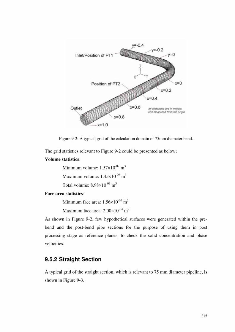
215
Figure 9-2: A typical grid of the calculation domain of 75mm diameter bend.
The grid statistics relevant to Figure 9-2 could be presented as below;
Volume statistics:
Minimum volume: 1.57×10-07 m3
Maximum volume: 1.45×10-06 m3
Total volume: 8.98×10-03 m3
Face area statistics:
Minimum face area: 1.56×10-05 m2
Maximum face area: 2.00×10-04 m2
As shown in Figure 9-2, few hypothetical surfaces were generated within the pre-
bend and the post-bend pipe sections for the purpose of using them in post
processing stage as reference planes, to check the solid concentration and phase
velocities.
9.5.2 Straight Section
A typical grid of the straight section, which is relevant to 75 mm diameter pipeline, is
shown in Figure 9-3.
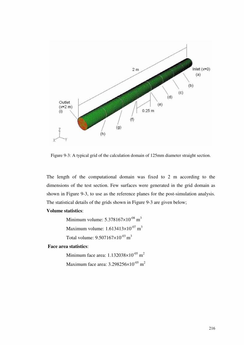
216
Figure 9-3: A typical grid of the calculation domain of 125mm diameter straight section.
The length of the computational domain was fixed to 2 m according to the
dimensions of the test section. Few surfaces were generated in the grid domain as
shown in Figure 9-3, to use as the reference planes for the post-simulation analysis.
The statistical details of the grids shown in Figure 9-3 are given below;
Volume statistics:
Minimum volume: 5.378167×10-08 m3
Maximum volume: 1.613413×10-07 m3
Total volume: 9.507167×10-03 m3
Face area statistics:
Minimum face area: 1.132038×10-05 m2
Maximum face area: 3.298256×10-05 m2
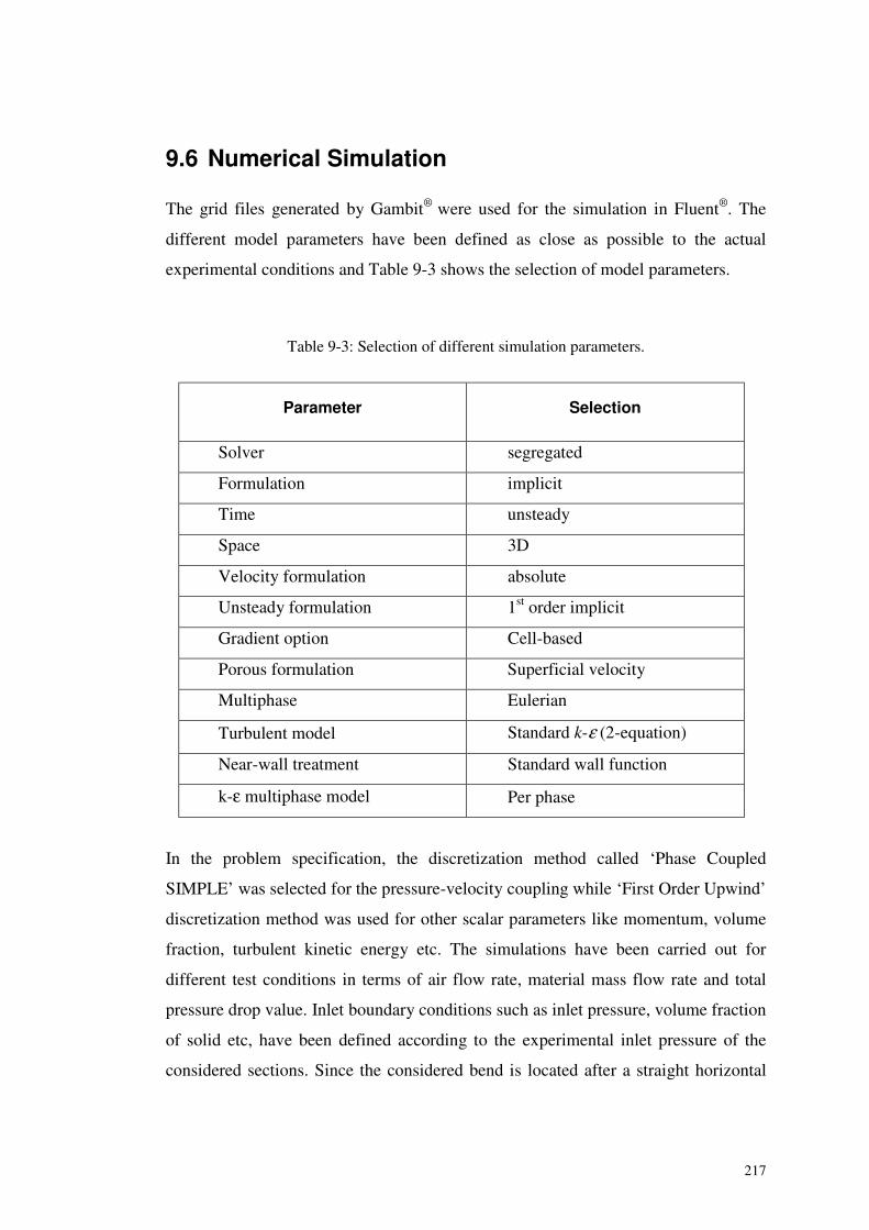
217
9.6 Numerical Simulation
The grid files generated by Gambit® were used for the simulation in Fluent®. The
different model parameters have been defined as close as possible to the actual
experimental conditions and Table 9-3 shows the selection of model parameters.
Table 9-3: Selection of different simulation parameters.
Parameter Selection
Solver segregated
Formulation implicit
Time unsteady
Space 3D
Velocity formulation absolute
Unsteady formulation 1st order implicit
Gradient option Cell-based
Porous formulation Superficial velocity
Multiphase Eulerian
Turbulent model Standard k-ε (2-equation)
Near-wall treatment Standard wall function
k-ε multiphase model Per phase
In the problem specification, the discretization method called ‘Phase Coupled
SIMPLE’ was selected for the pressure-velocity coupling while ‘First Order Upwind’
discretization method was used for other scalar parameters like momentum, volume
fraction, turbulent kinetic energy etc. The simulations have been carried out for
different test conditions in terms of air flow rate, material mass flow rate and total
pressure drop value. Inlet boundary conditions such as inlet pressure, volume fraction
of solid etc, have been defined according to the experimental inlet pressure of the
considered sections. Since the considered bend is located after a straight horizontal
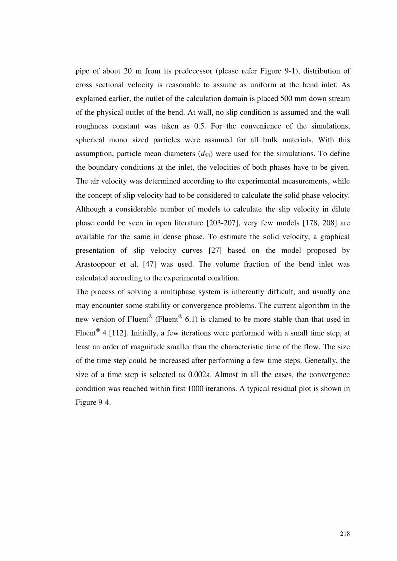
218
pipe of about 20 m from its predecessor (please refer Figure 9-1), distribution of
cross sectional velocity is reasonable to assume as uniform at the bend inlet. As
explained earlier, the outlet of the calculation domain is placed 500 mm down stream
of the physical outlet of the bend. At wall, no slip condition is assumed and the wall
roughness constant was taken as 0.5. For the convenience of the simulations,
spherical mono sized particles were assumed for all bulk materials. With this
assumption, particle mean diameters (d50) were used for the simulations. To define
the boundary conditions at the inlet, the velocities of both phases have to be given.
The air velocity was determined according to the experimental measurements, while
the concept of slip velocity had to be considered to calculate the solid phase velocity.
Although a considerable number of models to calculate the slip velocity in dilute
phase could be seen in open literature [203-207], very few models [178, 208] are
available for the same in dense phase. To estimate the solid velocity, a graphical
presentation of slip velocity curves [27] based on the model proposed by
Arastoopour et al. [47] was used. The volume fraction of the bend inlet was
calculated according to the experimental condition.
The process of solving a multiphase system is inherently difficult, and usually one
may encounter some stability or convergence problems. The current algorithm in the
new version of Fluent® (Fluent® 6.1) is clamed to be more stable than that used in
Fluent® 4 [112]. Initially, a few iterations were performed with a small time step, at
least an order of magnitude smaller than the characteristic time of the flow. The size
of the time step could be increased after performing a few time steps. Generally, the
size of a time step is selected as 0.002s. Almost in all the cases, the convergence
condition was reached within first 1000 iterations. A typical residual plot is shown in
Figure 9-4.
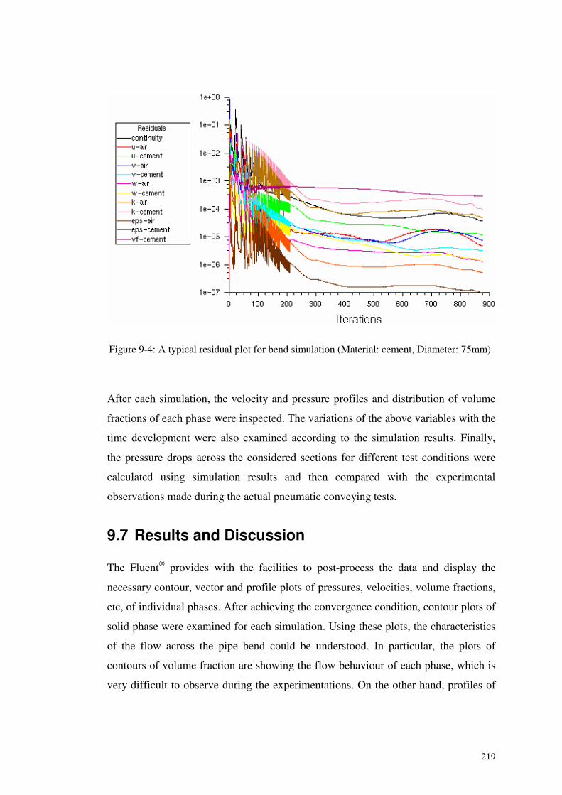
219
Figure 9-4: A typical residual plot for bend simulation (Material: cement, Diameter: 75mm).
After each simulation, the velocity and pressure profiles and distribution of volume
fractions of each phase were inspected. The variations of the above variables with the
time development were also examined according to the simulation results. Finally,
the pressure drops across the considered sections for different test conditions were
calculated using simulation results and then compared with the experimental
observations made during the actual pneumatic conveying tests.
9.7 Results and Discussion
The Fluent® provides with the facilities to post-process the data and display the
necessary contour, vector and profile plots of pressures, velocities, volume fractions,
etc, of individual phases. After achieving the convergence condition, contour plots of
solid phase were examined for each simulation. Using these plots, the characteristics
of the flow across the pipe bend could be understood. In particular, the plots of
contours of volume fraction are showing the flow behaviour of each phase, which is
very difficult to observe during the experimentations. On the other hand, profiles of
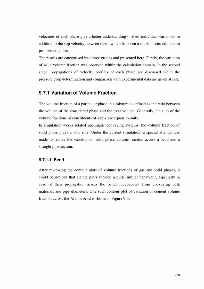
220
velocities of each phase give a better understanding of their individual variations in
addition to the slip velocity between them, which has been a much discussed topic in
past investigations.
The results are categorised into three groups and presented here. Firstly, the variation
of solid volume fraction was observed within the calculation domain. In the second
stage, propagations of velocity profiles of each phase are discussed while the
pressure drop determination and comparison with experimental data are given at last.
9.7.1 Variation of Volume Fraction
The volume fraction of a particular phase in a mixture is defined as the ratio between
the volume of the considered phase and the total volume. Generally, the sum of the
volume fractions of constituents of a mixture equals to unity.
In simulation works related pneumatic conveying systems, the volume fraction of
solid phase plays a vital role. Under the current simulation, a special attempt was
made to realize the variation of solid phase volume fraction across a bend and a
straight pipe section.
9.7.1.1 Bend
After reviewing the contour plots of volume fractions of gas and solid phases, it
could be noticed that all the plots showed a quite similar behaviour, especially in
case of their propagation across the bend, independent from conveying bulk
materials and pipe diameters. One such contour plot of variation of cement volume
fraction across the 75 mm bend is shown in Figure 9-5.
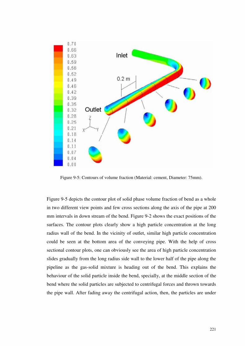
221
Figure 9-5: Contours of volume fraction (Material: cement, Diameter: 75mm).
Figure 9-5 depicts the contour plot of solid phase volume fraction of bend as a whole
in two different view points and few cross sections along the axis of the pipe at 200
mm intervals in down stream of the bend. Figure 9-2 shows the exact positions of the
surfaces. The contour plots clearly show a high particle concentration at the long
radius wall of the bend. In the vicinity of outlet, similar high particle concentration
could be seen at the bottom area of the conveying pipe. With the help of cross
sectional contour plots, one can obviously see the area of high particle concentration
slides gradually from the long radius side wall to the lower half of the pipe along the
pipeline as the gas-solid mixture is heading out of the bend. This explains the
behaviour of the solid particle inside the bend, specially, at the middle section of the
bend where the solid particles are subjected to centrifugal forces and thrown towards
the pipe wall. After fading away the centrifugal action, then, the particles are under
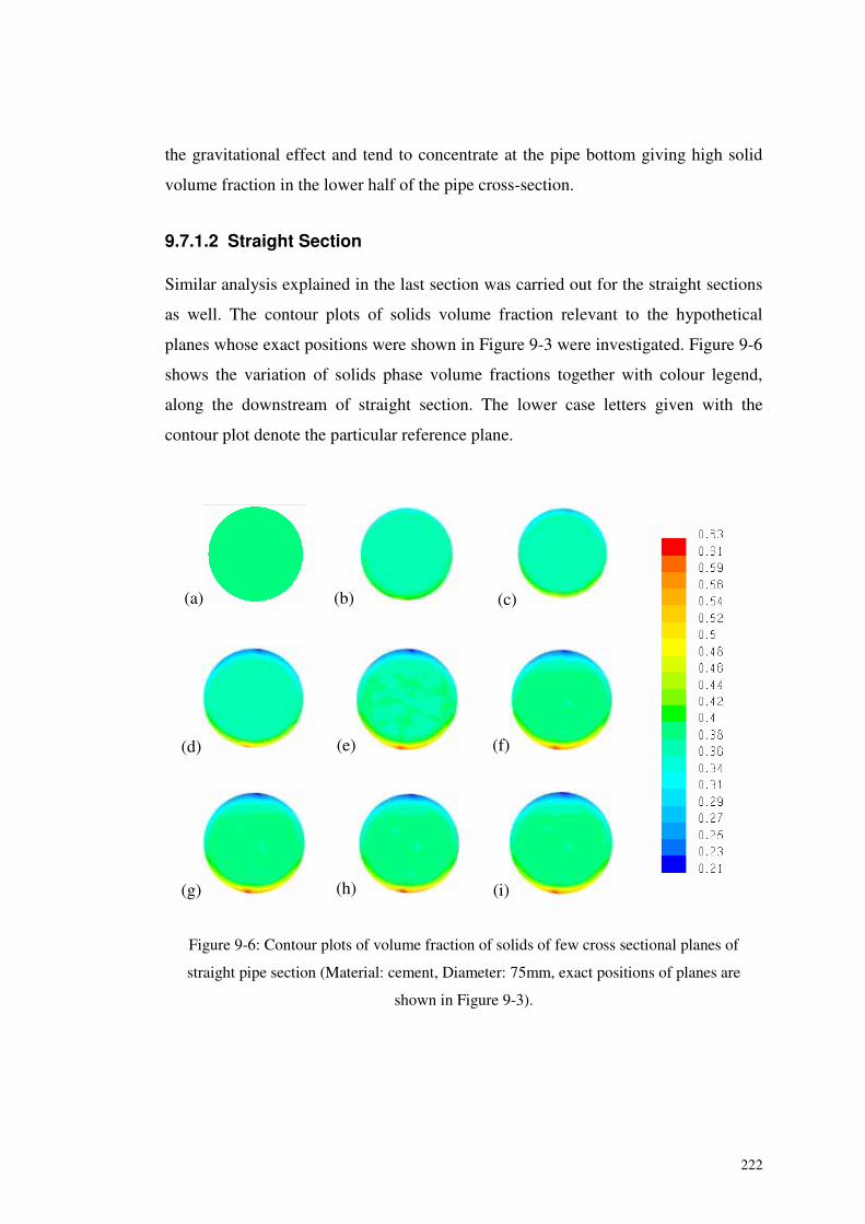
222
the gravitational effect and tend to concentrate at the pipe bottom giving high solid
volume fraction in the lower half of the pipe cross-section.
9.7.1.2 Straight Section
Similar analysis explained in the last section was carried out for the straight sections
as well. The contour plots of solids volume fraction relevant to the hypothetical
planes whose exact positions were shown in Figure 9-3 were investigated. Figure 9-6
shows the variation of solids phase volume fractions together with colour legend,
along the downstream of straight section. The lower case letters given with the
contour plot denote the particular reference plane.
Figure 9-6: Contour plots of volume fraction of solids of few cross sectional planes of
straight pipe section (Material: cement, Diameter: 75mm, exact positions of planes are
shown in Figure 9-3).
(a) (b) (c)
(d) (e) (f)
(g) (h) (i)
223
According to the series of contour plots, it is clear that when the flow negotiates the
downstream of the straight section, the solid concentration in the bottom region
gradually grows. Specially, a clear difference can be seen in the solid volume
fractions of the bottom and top region of the cross-section of the outlet region of the
straight section.
The similar phenomenon was reported in many other investigations [209-214] as
well. Most of them explained the presence of high solid fraction at the bottom of the
horizontal pipe wall as a result of gravitational settling of solids. Huber and
Sommerfeld [211] described it as a result of high loss of solids momentum at the
bottom of the pipe due to more intense particle-particle and particle-wall collisions as
compared to the upper portion of the pipe. They also found inelastic particle
collisions and viscous dissipation of the gas phase as the reasons for high momentum
loss. Some researchers [199, 209, 213, 215] have observed a characteristics of a rope
of solid particles inside and/or just downstream of a bend. Some of them also
reported a secondary flow pattern of a double vortex at the downstream of the bend.
However, these phenomena are quite common in dilute phase conveying where the
solid particles have more freedom to move. But, the flow modes under the
consideration of this investigation were completely in dense phase (the solid loading
ratio ranging from 29 to 257) according to the experimental observations discussed
in details in Section 4.6.2. Consequently, the solid particles have less freedom to
move around the conveying domain, thus the roping phenomenon may not be
applicable here.
9.7.2 Velocity profiles of gas and solid phase
In this stage, different aspects of velocities were examined using the post processing
facilities available in Fluent®. To understand the variations of gas and solid
velocities, the x-y plots of theses variables were examined along the pipeline. In spite
of conveying material and pipeline configuration, some common trends of velocity
distribution could be observed similar to the case of volume fractions. Figure 9-7
shows a typical graph of the variation of air and solid phase axial velocity profiles in
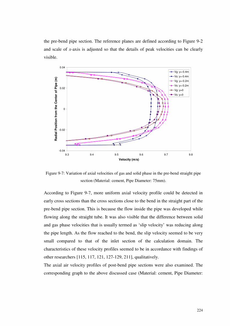
224
the pre-bend pipe section. The reference planes are defined according to Figure 9-2
and scale of x-axis is adjusted so that the details of peak velocities can be clearly
visible.
-0.04
-0.02
0
0.02
0.04
9.3 9.4 9.5 9.6 9.7 9.8
Velocity (m/s)
Rad
ialP
osi
tio
nfr
om
the
Cen
ter
of
Pip
e(m
)
Vg: y=-0.4m
Vs: y=-0.4m
Vg: y=-0.2m
Vs: y=-0.2m
Vg: y=0
Vs: y=0
Figure 9-7: Variation of axial velocities of gas and solid phase in the pre-bend straight pipe
section (Material: cement, Pipe Diameter: 75mm).
According to Figure 9-7, more uniform axial velocity profile could be detected in
early cross sections than the cross sections close to the bend in the straight part of the
pre-bend pipe section. This is because the flow inside the pipe was developed while
flowing along the straight tube. It was also visible that the difference between solid
and gas phase velocities that is usually termed as ‘slip velocity’ was reducing along
the pipe length. As the flow reached to the bend, the slip velocity seemed to be very
small compared to that of the inlet section of the calculation domain. The
characteristics of these velocity profiles seemed to be in accordance with findings of
other researchers [115, 117, 121, 127-129, 211], qualitatively.
The axial air velocity profiles of post-bend pipe sections were also examined. The
corresponding graph to the above discussed case (Material: cement, Pipe Diameter:
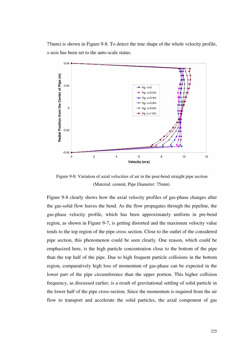
225
75mm) is shown in Figure 9-8. To detect the true shape of the whole velocity profile,
x-axis has been set to the auto-scale status.
-0.04
-0.02
0
0.02
0.04
0 2 4 6 8 10 12
Velocity (m/s)
Rad
ialP
osi
tio
nfr
om
the
Cen
ter
of
Pip
e(m
)
Vg: x=0
Vg: x=0.2m
Vg: x=0.4m
Vg: x=0.6m
Vg: x=0.8m
Vg: x=1.0m
Figure 9-8: Variation of axial velocities of air in the post-bend straight pipe section
(Material: cement, Pipe Diameter: 75mm).
Figure 9-8 clearly shows how the axial velocity profiles of gas-phase changes after
the gas-solid flow leaves the bend. As the flow propagates through the pipeline, the
gas-phase velocity profile, which has been approximately uniform in pre-bend
region, as shown in Figure 9-7, is getting distorted and the maximum velocity value
tends to the top region of the pipe cross section. Close to the outlet of the considered
pipe section, this phenomenon could be seen clearly. One reason, which could be
emphasized here, is the high particle concentration close to the bottom of the pipe
than the top half of the pipe. Due to high frequent particle collisions in the bottom
region, comparatively high loss of momentum of gas-phase can be expected in the
lower part of the pipe circumference than the upper portion. This higher collision
frequency, as discussed earlier, is a result of gravitational settling of solid particle in
the lower half of the pipe cross-section. Since the momentum is required from the air
flow to transport and accelerate the solid particles, the axial component of gas
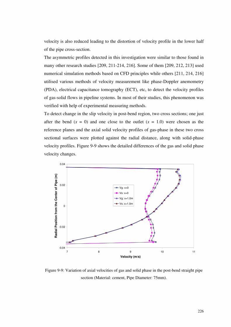
226
velocity is also reduced leading to the distortion of velocity profile in the lower half
of the pipe cross-section.
The asymmetric profiles detected in this investigation were similar to those found in
many other research studies [209, 211-214, 216]. Some of them [209, 212, 213] used
numerical simulation methods based on CFD principles while others [211, 214, 216]
utilised various methods of velocity measurement like phase-Doppler anemometry
(PDA), electrical capacitance tomography (ECT), etc, to detect the velocity profiles
of gas-solid flows in pipeline systems. In most of their studies, this phenomenon was
verified with help of experimental measuring methods.
To detect change in the slip velocity in post-bend region, two cross sections; one just
after the bend (x = 0) and one close to the outlet (x = 1.0) were chosen as the
reference planes and the axial solid velocity profiles of gas-phase in these two cross
sectional surfaces were plotted against the radial distance, along with solid-phase
velocity profiles. Figure 9-9 shows the detailed differences of the gas and solid phase
velocity changes.
-0.04
-0.02
0
0.02
0.04
7 8 9 10 11
Velocity (m/s)
Rad
ialP
osi
tio
nfr
om
the
Cen
ter
of
Pip
e(m
)
Vg: x=0
Vs: x=0
Vg: x=1.0m
Vs: x=1.0m
Figure 9-9: Variation of axial velocities of gas and solid phase in the post-bend straight pipe
section (Material: cement, Pipe Diameter: 75mm).
227
According to Figure 9-9, a clear difference could be seen between the gas and solid
velocity profiles corresponding to the cross section, which is just after the bend
curvature (x = 0), while the two profiles approximately coincide each other in the
cross section at further down stream (x = 1.0). Consequently, it is clear that the slip
velocity becomes less as the gas-solid mixture flows along the down-stream of the
bend. Similar features could be seen in pre-bend region as well. As the flow
approaches to the bend, the slip velocity becomes less as shown in Figure 9-7. This
demonstrates that the particle velocity is not very different from the gas velocity in
the developed flow. On the other hand, since the particles used for this investigation
is rather small, the possibility of experiencing a significant slip between two phases
is very less. However, the slip velocity is comparatively less, particularly, in dense
phase conveying conditions [6].
The concept of slip velocity or the velocity difference between phases has drawn a
special attention in research field of pneumatic conveying and considerable number
of publications could be found on this topic. Among them, some studies [47, 178,
203-208, 211] reported similar results to the current investigation.
9.7.3 Pressure drop determination
During the post processing of simulation data, it could be able to determine the
pressure drop across the considered bend. The pressure drops across the bend, mainly
in between the locations of two pressure transducers, were calculated with the help of
the simulation outcomes and compared with the experimental observations. Figure
9-10 shows the graph of experimental pressure drop values vs. calculated pressure
drop results for all three conveying materials in three different pipe sizes.
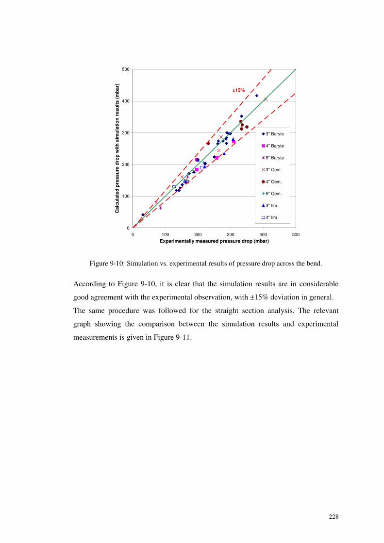
228
0
100
200
300
400
500
0 100 200 300 400 500
Experimentally measured pressure drop (mbar)
Cal
cula
ted
pre
ssu
red
rop
wit
hsi
mu
lati
on
resu
lts
(mb
ar)
3" Baryte
4" Baryte
5" Baryte
3" Cem
4" Cem.
5" Cem.
3" Ilm.
4" Ilm.
±15%
Figure 9-10: Simulation vs. experimental results of pressure drop across the bend.
According to Figure 9-10, it is clear that the simulation results are in considerable
good agreement with the experimental observation, with ±15% deviation in general.
The same procedure was followed for the straight section analysis. The relevant
graph showing the comparison between the simulation results and experimental
measurements is given in Figure 9-11.
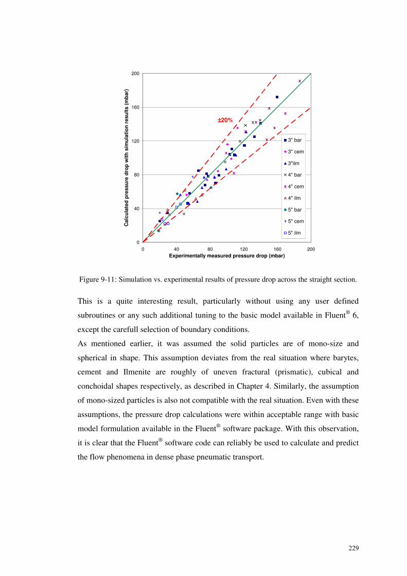
229
0
40
80
120
160
200
0 40 80 120 160 200Experimentally measured pressure drop (mbar)
Cal
cula
ted
pre
ssu
red
rop
wit
hsi
mu
lati
on
resu
lts
(mb
ar)
3" bar
3" cem
3"ilm
4" bar
4" cem
4" ilm
5" bar
5" cem
5" ilm
±±±±20%
Figure 9-11: Simulation vs. experimental results of pressure drop across the straight section.
This is a quite interesting result, particularly without using any user defined
subroutines or any such additional tuning to the basic model available in Fluent® 6,
except the carefull selection of boundary conditions.
As mentioned earlier, it was assumed the solid particles are of mono-size and
spherical in shape. This assumption deviates from the real situation where barytes,
cement and Ilmenite are roughly of uneven fractural (prismatic), cubical and
conchoidal shapes respectively, as described in Chapter 4. Similarly, the assumption
of mono-sized particles is also not compatible with the real situation. Even with these
assumptions, the pressure drop calculations were within acceptable range with basic
model formulation available in the Fluent® software package. With this observation,
it is clear that the Fluent® software code can reliably be used to calculate and predict
the flow phenomena in dense phase pneumatic transport.
230
9.8 Conclusion
The Euler-Euler granular approach with the kinetic theory for the multiphase flow
has been used to simulate the gas-solid particle flow in a standard 90º horizontal to
horizontal bend and a straight pipe section of 2m long of a pneumatic transport
system with dense phase flow condition, using a commercial CFD software package;
Fluent® in three-dimensional space. To simulate the turbulence for the gas and solid
phases, the k-ε model has been used. Pneumatic conveying tests were carried out
using three different materials and three different pipeline configurations with
respect to the pipe diameter.
The results on variations of volume fraction of solid particle, gas and solid phase
velocity profiles and pressure drop determination across the bend were analysed
using the post-processing facilities available with the software. Although no
experimental measurement was made on solid particle concentrations and phase
velocities, a good qualitative agreement of the simulation results could be detected
with the published results by other research workers. In case of pressure drop
determination, considerably good agreement could be found between the
experimental measurements and simulation results with error margins of ± 15% for
the bends and ± 20% for the straight sections for all conveying conditions and
combinations under the consideration of this investigation.
From the simulation results, it is clear that Fluent® CFD software has a good
potential to model the gas-sold flow across a bend in dense phase pneumatic
conveying satisfactorily. In fact, this investigation and the simulation work have been
carried out as an initial step towards a reliable modelling technique of dense phase
pneumatic conveying.
231
10 CONCLUSIONS AND SUGGESTIONS FORFUTURE WORK
10.1 Introduction
As discussed in details under Chapter 1, the main aim of the present investigation
was to formulate a comprehensive scaling up technique for pneumatic conveying
system designs. The investigation was conducted in few steps addressing different
important issues separately and formulating the models to explain the behaviour of
gas-solid flow in various sections of conveying line. In the final stage, all proposed
models were put together in the form of a computer based software programme. In
addition, a detailed investigation was carried out to check the ability of a commercial
software; Fluent® based on computational fluid dynamics principles, to use as a tool
for pressure drop prediction across different pipeline components.
Under this chapter, the general conclusions based on the findings of the present
investigation are discussed followed by the conclusions drawn in respect of;
• Scaling up of line pressure drop
• Scaling up of entry loss
• Scaling up of minimum conveying conditions
• Numerical simulations
At the end, suggestions are made for the continuation of this scientific investigation
leading to a better understanding and control of pneumatic conveying systems.
10.2 General Conclusions
As mentioned under Chapter 1, this investigation was planned on the basis of the
findings of a preliminary investigation [29], where the capabilities of available
scaling up and pressure drop prediction models of pneumatic conveying systems
were discussed. According to the said investigation, the available scaling up
techniques were found to over-estimate the pressure drop, in most of the cases. This,
in other words, implies that the material transport capacity of the system is
232
underestimated for a particular available pressure head. The literature survey carried
out with the aim of exploring the current status of pneumatic conveying field in the
light of modern scientific studies, also revealed the lack of scaling up and pressure
drop predicting techniques, which are simple, straight forward, complete and reliable
in their applications of both dilute and dense phase conveying. The above described
findings indicated a need for a scientific study to investigate the possibilities of
formulating a comprehensive scaling up technique.
The research investigation presented in this thesis is believed to be an important
contribution to the knowledge in the field of pneumatic conveying. This is the first
time that all the aspects and components of conveying line together with the
minimum conveying conditions are addressed in scaling up standpoint. A number of
important conclusions, as described in individual sections, have been drawn from the
pneumatic conveying tests and the model formulations for scaling up methods.
10.2.1 Scaling up of Line Pressure Drop
This section basically addressed the conveying line starting from the outlet section of
the blow tank to the inlet section of receiving tank including all types of bends,
together with all pipeline accessories like valves, hose sections, etc,. The pneumatic
conveying test runs were carried out with five different bulk materials including one
with five different qualities in terms of mean particle diameter and particle size
distribution. Five different configurations of conveying pipelines were used during
the tests. Attempt was made to cover the whole range of conveying conditions, i.e.,
from dilute phase to dense phase for all the materials tested.
A model was proposed based on the well-known piece wise approach of scaling. The
piece wise approach, as understood by many other researchers as well, gives
comparatively better results than in the case of global approach, where the whole
conveying line is considered as a single unit with all bends and other accessories on
it, since the positions of individual features of pipeline are taken into account
together with their inlet velocities. One can easily understand the importance of the
inlet velocities of different sections, since it varies along the pipeline and the
233
behaviour of gas-solid flow is greatly influenced by the inlet velocity of the
concerned section.
The proposed model is a modified version of the well-known Darcy-Weisbach’s
equation for single phase flows. The friction factor is replaced with a newly
introduced factor called ‘pressure drop coefficient’ or K factor and the density term is
also replaced by suspension density as defined in Section 4.2.2.
The properties of K factor and the relevant conclusions could be listed as follows.
• After plotting the K factors against few different parameters, it was revealed
that there is a strong relationship between K value of straight pipe sections
and other pipe accessories like bends, valves, etc, and the square value of
entry velocity of the concerned section.
• The behaviour of K vs. Ventry2 curves shows a common trend of power-law
relationship with increasing entry velocity for all conveying bulk materials.
This leads to a conclusion that the value of K factor decreases rapidly with
increase in conveying velocity for dense phase conditions, where the
conveying velocity is low and attains more or less a constant value for the
dilute phase conveying condition.
• The relationship between K and Ventry2 is found to be independent of pipe
diameter for all pipe sections and all conveying materials tested in this study.
• The behaviour of K vs. Ventry2 for horizontal pipe sections was found to be
dependent on the mean particle size of the conveying material, while the
same for vertical pipe sections was found to be independent of particle size.
• In the validation analysis using graphical and statistical tools, all possible
combinations of pipeline configurations, bulk materials and flow conditions
were used and it showed a reasonably good agreement between predicted and
experimentally measured pressure values along the conveying pipeline. This
is considered to be a significant achievement.
• The predictions of proposed model were compared with some popular scaling
up and pressure drop determination techniques available the literature. The
scaling up technique proposed in this thesis gave the least error in all flow
conditions considered.
234
10.2.2 Scaling up of Entry Loss
During the conveying tests with different materials and pipeline configurations, it
was noticed that the pressure loss incurred at the entry section of the conveying line
is significant, especially in case of top discharge blow tank systems. Under the
present investigation, a model was derived using dimensional analysis for scaling up
of entry pressure loss in a top discharge blow tank. The model developed was found
to be independent of pipe size and hence could be used as a very useful tool for
scaling up. The proposed model is very simple and needs only readily available
experimental data without any complicated manipulation. The validation analysis
showed very promising results for different conveying materials, pipeline
configurations and flow conditions tested.
10.2.3 Scaling up of Minimum Conveying Velocity
The determination of minimum conveying velocity is crucial for the successful
operation of a pneumatic conveying system. It was found that the available models
did not give reliable predictions, especially for fine powders.
The major problem for formulating a general model for minimum conveying velocity
has been identified as the availability of numerous influential parameters such as,
particle size and size distribution, particle density, particle shape, gas density, etc.
During the present investigation, the mathematical techniques called principal
component analysis and dimensional analysis were successfully used to screen out
the influential parameters and formulate a relationship between the most important
physical parameters of the minimum conveying velocity. The validation and
comparison analysis showed a good agreement between the predictions of proposed
model and experimentally observed minimum conveying conditions.
10.2.4 Computer Based Calculation Programme
Having developed all the models, i.e., conveying line pressure drop for straight
sections, bends, valves, etc, entry pressure drop, minimum conveying velocity
235
prediction, an attempt was made to develop a general computer based calculation
programme. The calculation in the programme is done in steps of 1 m pipe sections
for straight pipe sections. However, valves bends and other pipe components are
considered as individual sections in calculation programme.
Using the test plant results for each material, one can have a general system design
programme for that material for any variations of pipe size, transport capacity, air
pressure and air flow rate. The calculation programme has been tested for all the
materials under this study.
10.2.5 CFD Simulation on Pipe Bends and Straight
Sections
As an alternative approach to the classical methods of pressure drop determination
using various models, the numerical simulation technique using computational fluid
dynamics (CFD) principles has also been tried in this study. The basic objective of
the inclusion of numerical simulation component to this experimental study was to
find out whether the commercially available CFD software codes are good enough to
predict the pressure drop of a pneumatic transport system reliably.
The Euler-Euler granular approach with the kinetic theory for the multiphase flow
was used to simulate the gas-solid particle flow in a standard 90º horizontal to
horizontal bend and a straight section of 2m long of a pneumatic transport system
with dense phase flow condition, using a commercial CFD software package, called
Fluent®, in three-dimensional space. The turbulence of gas and solid phases was
modelled using the k-ε model. The results produced by three different conveying
materials and three different pipeline configurations were used for the simulation
work.
With the help of the post-processing facilities of considered software, the results on
variations of volume fraction of solids particle, gas and solid phase velocity profiles
and pressure drop determination across the bend were analysed. During the
experimentations, measurements were not made on solid particle concentrations and
phase velocities. But, the results of numerical simulations were seen in a good
236
qualitative agreement with the published results by other research workers. In case of
pressure drop determination, a good agreement could be found between the
experimental measurements and simulation results with error margins of ± 15% for
the bends and ± 20% for the straight sections for all conveying conditions and for all
combinations of conveying materials and pipe configurations considered. This is a
considerable achievement amidst the divergent disagreements reported in literatures.
10.3 Suggestion for Future Works
Although the models proposed under the present investigation have been remarkably
successful for the different materials and pipeline configurations tested, it has been
understood that there are still many aspects that have not been fully addressed. There
are some areas where further scientific studies and investigations would further
improve our general understanding of the complex flow phenomenon of pneumatic
conveying. The followings are some suggestions for future studies.
• Although the scaling up models produce very good results for conveying
materials selected for the current investigation, more experiments need to be
undertaken to cover an even wider range of bulk materials. Since the selected
materials are mostly representing the group ‘A’ and ‘C’ materials of Geldart
classification, the testing of bulk materials of other groups are recommended.
• One shortcoming of the measurement procedure adopted during the current
investigation was that the re-acceleration pressure drops related to bends and
other pipe components did not taken into account. The modifications are
recommended for the measurement procedure and the effect of re-
acceleration of flow has to be determined.
• The inclusion of vertical sections of 125 mm pipe diameter is also
recommended.
• The pressure drop coefficient or K factor has been found to be dependent on
the material quality. It will be interesting to investigate if it is possible to
predict the K factor based on material characteristics.

237
• In the proposed models, the mean particle diameter or d50 has been used
instead of particle size distribution. Attempt should be made to incorporate
the effects of particle side distribution in the proposed models.
• The effect of particle shape on pressure drop will also be interesting to
investigate.
• It is suggested that further studies should be made for the applicability of
CFD simulation technique for various other types of bends, pipe components
and vertical sections.

238
11BIBLIOGRAPHY
1. Purutyan, H., T.G. Troxel, and F. Cabrejos, Propel your pneumatic conveying
system to higher efficiency. Chemical Engineering Progress, 2001. 97(4): p.
42-55.
2. Woodcroft, B. The pneumatics of hero of Alexandria. 1851 [cited 2005;
Available from: http://www.history.rochester.edu/steam/hero/.
3. Wypych, P.W., Introduction to Pneumatic Conveying. Transport of
Particulate Materials, An Intensive Short Course, Porsgruun, Norway, 1999.
4. Molerus, O., Overview: Pneumatic Transport of Solids. Powder technology,
1996. 88(3): p. 309-321.
5. Huggett, M.R. The Evalution of the Practice of Pneumatic Conveying. in
Pneumatech 3, Third International Conference on Pneumatic Conveying
Technology. 1987. The Grand Hotel, Jersey, Channel Islands.
6. Klinzing, G.E., Marcus, R.D., Rizk, F. and Leung, L.S., Pneumatic
Conveying of Solids -A Theoretical and Practical Approach. 1997: Chapman
& Hall.
7. Soo, S.L., Long Distance Pneumatic Transportation. Journal of Pipelines,
1984. 4: p. 79-85.
8. Link, W.H., 1998, Investigation of the Efficacy of the Flow Enhancer and the
Indentification of the Beginning of the Unstable Zone in Pneumatic
Conveying Systems, Graduate Faculty, School of Engineering, University of
Pittsburgh, Pittsburgh, USA.
9. AIR-TEC System: Official Website,
http://www.air-tec.it/index_materialitrasp_uk.html
10. Zapato, L., The Inteli-Tube Pneumatic Transportation System.
11. Liu, H. Pneumatic Casule Pipeline- Basic Concept, practical Considerations,
and Current Research. in Mid-Continent Transportation Symposium. 2000.
Iowa State University, Ames, Iowa, USA.
239
12. De Silva, S.R. and B.K. Datta, Transport of Particulate Materials- Dilute
Phase Pneumatic Transport, in Lecture Notes on Powder Technology,
Telemark University College, Porsgruun, Norway. 2000.
13. The Basics of Pneumatic Conveying, 2004,
http://www.dynamicair.comsystems.html
14. Zenz, F.A., Conveyability of Materials of Mixed Particle Size. Industrial and
Engineering Chemistry, American Chemical Society, 1964. 3(1): p. 65-75.
15. Zenz, F.A. and D.F. Othmer, Fluidization and fluid particle systems. 1960:
Reinhold, New York.
16. Mills, D., Pneumatic Conveying Design Guide. 1990: Butterworth.
17. Mills, D., Optimizing pneumatic conveying. Chemical Engineering, 2000.
107(13): p. 74-80.
18. Mills, D., A review of the research work of Professor Predrag Marjanovic.
Chemical Engineering and Processing, 2005. 44(2): p. 141-151.
19. Mills, D. and J.S. Mason, The Uprating of Pneumatic Conveying Systems.
Journal of Pipelines, 1982. 2(2-4): p. 199-210.
20. Mills, D. and J.S. Mason. The influence of conveying distance on the
performance and air requiremnts of pneumatic conveying system pipelines. in
Reliable Flow of Particulate Soilds. 1985. Bergen, Norway.
21. Behera, S. and S. Das, Desirable conveying characteristics for pneumatic
transportation of fly-ash, sand, cement and crushed bath. Powder Handling &
Processing, 2000. 12(1): p. 23-25.
22. Pan, R. and P.W. Wypych, Scale-up Procedures for Pneumatic Conveying
Design. Powder Handling and Processing, 1992. 4(2): p. 167-172.
23. Pan, R. and P.W. Wypych, Pressure Drop and Slug Velocity in Low-Velocity
Pneumatic Conveying of Bulk Solids. Powder Technology, 1997. 94(2): p.
123-132.
24. Wypych, P.W., Prediction and Scaling up of Steady-State Operating
Condition. Transport of Particulate Materials, An Intensive Short Course,
Porsgruun, Norway, 1999.
240
25. Wypych, P.W. and P.C. Arnold, On Improving Scale-up Procedures for
Pneumatic Conveying Design. Powder Technology, 1987. 50(3): p. 281-294.
26. Klinzing, G.E., N.D. Rohatgi, A. Zaltash, and C.A. Myler, Pneumatic
Transport - a Review (Generalized Phase-Diagram Approach to Pneumatic
Transport). Powder Technology, 1987. 51(2): p. 135-149.
27. Woodcock, C.R. and J.S. Mason, Bulk Solids Handling - An Introduction to
the Practice and Technology. 1987: Leonard Hill.
28. Meyers, S., R.D. Marcus, and F. Rizk, The state diagrame for fine-particle
gas/solids suspensions. Bulk Solids Handling, 1985. 5(4): p. 779-782.
29. Ratnayake, C., 2000, An Experimental Investigation of Scaling Up
Techniques in Pneumatic Conveying, MSc, Dept. of Powder Science and
Technology, Telemark University College, Porsgrunn, Norway.
30. De Silva, S.R., Transport of Particulate Material- Dilute Phase Pneumatic
Transport. Lecture Notes on Powder Technology, Telemark University
College, Porsgruun, Norway, 1995.
31. Mills, D., Troubleshooting Pneumatic Conveying.2. Major Systems and Their
Key Components. Chemical Engineering, 1990. 97(7): p. 101-107.
32. Marcus, R.D., C. Wiggill, and F. Rizk, Parameters Influencing Long-
Distance Pneumatic Conveying Systems. The Best of Powder Handling &
Processing Bulk Solids Handling, 1985. D/86: p. 17-24.
33. Jones, M.G., D. Mills, and J.S. Mason, A Comparison of the Performance of
Top and Bottom Discharge Blow Tank Systems. Bulk Solids Handling, 1987.
7(5): p. 701 - 706.
34. Cabrejos, F.J. and G.E. Klinzing, Incipient Motion of Solid Particles in
Horizontal Pneumatic Conveying. Powder Technology, 1992. 72(1): p. 51-61.
35. Cabrejos, F.J. and G.E. Klinzing, Pickup and saltation mechanisms of solid
particles in horizontal pneumatic transport. Powder technology, 1994. 79(2):
p. 173-186.
36. Martinussen, S.E., 1996, The Influence of the Physical Characteristics of
Particulate Materials on their Conveyability in Pneumatic Transport
241
Systems, PhD, Technological Department, Telemark University College,
Porsgruun, Norway.
37. Matsumoto, S., Hara, M., Saito, S., Maeda, S., Minimum Transport Velocity
for Horizontal Pneumatic Conveyimg. Journal of Chemical Engineering,
Japan, 1974. 7(6): p. 425-430.
38. Rizk, F., Pneumatic Conveying at Optimal Conditions and a Solution of
Barth's Equation. Pneumotransport 3, Third International Conference on the
Pneumatic Transport of Solids in Pipes, 1976. Paper D4: p. 43-58.
39. Rizk, F., Pneumatic Transport in Dilute and Dense Phase. Bulk Solids
Handling, 1982. 2(2): p. 9-15.
40. Woodcock, C.R., Review of Latest Theoretical Studies. Course on Advanced
Pneumatic Conveying, Copenhagen, Denmark.
41. Weber, M., Correlation Analyses in the Design of Pneumatic Transport
Plant. Bulk Solids Handling, 1982. 2(2): p. 231-233.
42. Pan, R. and J. Chambers, Pneumatic Conveying of Iron Ore in a High
Pressure System -Part B: Details of Test Runs and Scale-up Procedures.
Bulk Solids Handling, 1999. 19(3): p. 321-327.
43. Weber, M., Friction of the Air and Air/Solid Mixture in Pneumatic
Conveying. Bulk Solids Handling 2, 1991. 11(1): p. 99-102.
44. Massey, B.S., Mechanics of Fluids. 6th Edition ed. 1989: Van Nostrand
Reinhold.
45. Streeter, V.L. and E.B. Wylie, Fluid Mechanics, ed. s. metric: McGraw Hill.
46. Wypych, P.W. and R. Pan, Determination of Air-only pressure Drop in
Pneumatic Conveying Systems. Powder Handling and Processing, 1991. 3(4).
47. Arastoopour, H., M.V. Modi, D.V. Punwani, and A.T. Talwalkar. A Review
of Design Equations for the Dilute-Phase Gas-Solids Horizonntal Conveying
Systems for Coal and Related Materials. in Proc. of International Powder
and Bulk Solids Handling and Processing Conference. 1979. Philadelphia.
48. Rose, H.E. and H.E. Barnacle, Flow of Suspensions of Non-cohesive
Spherical Particles in Pipes. The Engineer, 1957. 203: p. 898-901.
242
49. Hinkle, B.L., Acceleration of Particle and Pressure Drop Encountered in
Horizontal Pneumatic Conveying. PhD Thesis, Georgia Institute of
Technology, 1953.
50. Richardson, J.F. and M. McLeman, Pneumatic Conveying: Part II; Solids
Velocities and Pressure Gradients in a One-inch Horizontal Pipe.
Transactions of Institution of Chemical Engineers, 1960. 38: p. 257-266.
51. Boothroyd, R.G., Flowing Gas-Solids Suspensions. 1971: Chapman and Hall,
London.
52. Yang, W.C., Correlations of Solid Friction Factors in Vertical and
Horizontal Pneumatic Conveying. AiChE Journal, 1974. 20(3): p. 605-607.
53. Szikszay, G., Friction factor for Dilute Phase Pneumatic Conveying. Bulk
Solids Handling 2, 1988. 8(4): p. 395-399.
54. Pan, R. and P.W. Wypych, Pressure Drop Due to Solids-Air Flow in
Horizontal and Vertical Pipes. Proc. of International Conference on Bulk
Material Handling &Transportation; Symposium on Freight Pipelines,
Wollongong, Australia, 1992.
55. Duckworth, R.A., Empirical Correlations for the Dilute Phase. Lecture
Notes, C.S.I.R.O. mineral Engineering, Dept. Of Chemical Engineering,
Univ. of Queensland.
56. Stermerding, S., The Pneumatic Transport of Cracking Catalist in Vertical
risers. Chemical Engineering Science, 1962. 17(8): p. 599-608.
57. Reddy, K.V.S. and D.C.T. Pei, Particle Dynamics in Solids-Gas Flow in a
vertical Pipe. Industrial Engineering Chemical Fundamental, 1969(8): p. 490.
58. Capes, C.E. and K. Nakamura, Vertical Pneumatic Conveying: An
Experimental Study with Particles in Intermediate and Turbulent Flow
Regimes. Canadian Journal of Chemical Engineering, 1973. 51: p. 31.
59. Konno, H. and S. Saito, Pneumatic Conveying of Soilds through Straight
Pipes. Journal of Chemical Engineering, Japan, 1969. 2(2): p. 211.
60. Klinzing, G.E., C.A. Myler, A. Zaltash, and S. Dhodapkar, A Simplified
Correlation for Solids Friction Factor in Horizontal Conveying Systems
243
Based on Yang's Unified Theory. Powder Technology, 1989. 58(3): p. 187-
193.
61. Molerus, O. and U. Heucke, Pneumatic Transport of Coarse Grained
Particles in Horizontal Pipes. Powder Technology, 1999. 102(2): p. 16.
62. Mills, D., D.J. Mason, and V.K. Agarwal, An Accesment of Acceleration
Length through Erosive Measurements. Proc. of 10th Annual Conference on
Powder & Bulk Solids Handling and Processing, Rosemont, Illinois, 1985: p.
215-228.
63. Marcus, R.D., Pneumatic Conveying of Bulk Solids. Notes of Short Courses
on Pneumatic Conveying, The Univ. of Newcastle, NSW, Australia, 1983.
64. Konrad, K., D. Harrison, R.M. Neddermann, and J.F. Davidson, Prediction of
the Pressure Drop for Horizontal Dense Phase Conveying of Particles.
Pneumotransport 5, Proc. of 5th International Conference on the Pneumatic
Transport of Solids in Pipes, London, UK., 1980: p. 225-244.
65. Konrad, K., Dense-Phase Pneumatic Conveying through Long Pipelines:
Effect of Significantly Compressible Air Flow on Pressure Drop. Powder
Technology, 1986. 48(3): p. 193-203.
66. Legel, D. and J. Schwedes, Investigation of Pneumatic Conveying of Plugs of
Cohesionless Bulk Solids in horizontal Pipes. Bulk Solids Handling, 1984.
4(2): p. 399-405.
67. Mi, B. and P.W. Wypch, Pressure-Drop Prediction in Low-Velocity
Pneumatic Conveying. Powder Technology, 1994. 81(2): p. 125-137.
68. Mi, B. and P.W. Wypych, Investigations into Wall Pressure during Slug-
Flow Pneumatic Conveying. Powder Technology, 1995. 84(1): p. 91-98.
69. Pan, R., B. Mi, and P.W. Wypych, Pneumatic Conveying Characteristics of
Fine and Granular Bulk Solids. KONA, 1994. 12: p. 77-85.
70. Matsuda, M., N. Sugita, S. Nihimori, N. Sugimoto, and Y. Morikawa, Dense
Phase Flow of Powder in Horizontal and Inclined Pneumatic Conveying by a
Nemo Pump. Powder Handling and Processing, 2000. 12(1): p. 17-21.
244
71. Hong, J., Y.S. Shen, and S.L. Liu, A Model for Gas-Solid Stratified Flow in
Horizontal Dense-Phase Pneumatic Conveying. Powder Technology, 1993.
77(2): p. 107-114.
72. Woodcock, C.R., Mason, J.S., Bulk Solids Handling - An Introduction to the
Practice and Technology. 1987: Leonard Hill.
73. Werner, D., Influence of Particle Size Distribution during Pneumatic Dense
Phase Conveying in Vertical and Horizontal Pipes. Bulk Solids Handling,
1983. 3(2): p. 351-359.
74. Plumpe, J.G., C. Zhu, and S.L. Soo, Measurements of Fluctuations in Motion
of Particles in a dense phase gas/solid suspension in vertical pipe flow.
Powder Technology, 1993. 77(2): p. 209-214.
75. Rautiainen, A., G. Stewart, V. Poikolainen, and P. Sarkomaa, An
Experimental Study of Vertical Pneumatic Conveying. Powder Technology,
1999. 104(2): p. 139-150.
76. Tsuji, Y. and R. Asano, Fundamental investigation of plug conveying of
cohesionless particles in a vertical pipe (pressure drop and friction of a
stationary plug). The Canadian Journal of Chemical Engineering, 1990. 68:
p. 758/767.
77. Yang, W.C., Correlation for Solid Friction Factor in Vertical Pneumatic
Conveying Lines. AIChE Journal, 1978. 24(3): p. 548-552.
78. Carpinlioglu, M.O., T.A. Ozbelge, and V. Oruc, Flow frictional resistance in
pneumatic conveying of solid particles through inclined lines. Powder
Technology, 2002. 125(2-3): p. 292-297.
79. Ginestet, A., P. Guigon, J.F. Large, and J.M. Beeckmans, Further-Studies on
Flowing Gas-Solids Suspensions in a Tube at High Angles of Inclination.
Canadian Journal of Chemical Engineering, 1994. 72(4): p. 582-587.
80. Hirota, M., Y. Sogo, T. Marutani, and M. Suzuki, Effect of mechanical
properties of powder on pneumatic conveying in inclined pipe. Powder
Technology, 2002. 122(2-3): p. 150-155.
81. Levy, A., T. Mooney, P. Marjanovic, and D.J. Mason, A Comparison of
Analytical and Numerical Models with Experimental Data for Gas-Solid
245
Flow through a Straight Pipe at Different Inclinations. Powder Technology,
1997. 93(3): p. 253-260.
82. Aziz, Z.B. and G.E. Klinzing, Dense Phase Plug Flow Transfer:The 1-inch
Horizontal Flow. Powder Technology, 1990. 62: p. 41-49.
83. Ito, H., Pressure losses in smooth pipe bends. Journal of Basic Engineering,
1960(March): p. 131-143.
84. Mills, D. and M.J. Mason, The Influence of Bend geometry on Pressure Drop
in Pneumatic Conveying System Pipelines. Proceedings of 10th Annual
Conference on Powder and Bulk Solids Handling and Processing. Rosemont.
Illinois., 1985: p. 203-214.
85. Klinzing, G.E., A comparison of pressure losses in bends between recent data
and model for gas-solid flow. The Canadian journal of chemical engineering,
1980. 58: p. 670-672.
86. Pan, R., P.W. Wypych, and P.C. Arnold, Pressure Drop due to different
Radius Bends connected by Short Straight Pipes. Proceedings of International
Symposium 'RELPOWFLO II'. Oslo. Norway, 1993: p. 1022-1029.
87. Westman, M.A., E.E. Michaelides, and F.M. Thomson, Pressure Losses Due
to Bends in Pneumatic Conveying. Journal of Pipelines, 1987. 7(1): p. 15-20.
88. Marcus, R.D., J.D. Hilbert, and G.E. Klinzing, The Flow through Bends in
Pneumatic Conveying Systems. Journal of Pipelines, 1984. 4(2): p. 103-112.
89. Cabrejos, F.J. and G.E. Klinzing, Minimum Conveying Velocity in Horizontal
Pneumatic Transport and the Pickup and Saltation Mechanisms of Solid
Particles. Bulk Solids Handling, 1994. 14(3): p. 541.
90. Hayden, K.S., K. Park, and J.S. Curtis, Effect of Particle Characteristics on
Particle Pickup Velocity. Powder Technology, 2003. 131: p. 7-14.
91. Molerus, O., Principles of flow in disperse systems. 1993: Chapman & Hall.
92. Weber, M., Principles of Hydraulic and Pneumatic Conveying in Pipes. The
Best of the Bulk Solids handling 1981-85, Pneumatic Conveying of bulk &
Powder., 1981. D86: p. 1- 7.
246
93. Xu, G.W., K. Nomura, S. Gao, and K. Kato, More fundamentals of dilute
suspension collapse and choking for vertical conveying systems. Aiche
Journal, 2001. 47(10): p. 2177-2196.
94. Yang, W.C., A Mathematical Definition of Choking Phenomenon and a
Mathematical Model for Predicting Choking Velocity and Choking Voidage.
AIChE Journal, 1975. 21(5): p. 1013 - 1015.
95. Keys, S. and A.J. Chambers. Scaling Pneumatic Conveying Characteristics
for Pipeline Pressure. in International Symposium: Reliable Flow of
Particulate Solids II. 1993. Oslo, Norway.
96. Bradley, M.S.A., pressure Losses Caused by Bends in Pneumatic Conveying
Pipelines -Effects of Bend Geometry and Fittings. Powder Handling and
Processing, 1990. 2(4): p. 315-321.
97. Bradley, M.S.A. and A. Reed, An Improved Method of Predicting Pressure
Drop Along Pneumatic Conveying Pipelines. Powder Handling & Processing,
1990. 2(3): p. 223-227.
98. Hettiaratchi, K., M.S.A. Bradley, R.J. Farnish, I. Bridle, L.M. Hyder, and
A.R. Reed, An investigation into the effect of product type when scaling for
diameter in vertical pipelines. Powder Technology, 2000. 112(3): p. 229-234.
99. Hettiaratchi, K., M.S.A. Bradley, A.R. Reed, and M.J. Smith, Pressure drop
in pneumtic conveying through vertical pipelines. BULK MAT. HANDL. &
TRANSP., 1992(July 6, - 8.): p. 73 - 77.
100. Hyder, L.M., M.S.A. Bradley, A.R. Reed, and K. Hettiaratchi, An
investigation into the effect of particle size on straight-pipe pressure
gradients in lean-phase conveying. Powder Technology, 2000. 112(3): p.
235-243.
101. Reed, A. and M.S.A. Bradley, Advances in the Design of Pneumatic
Conveying Systems - A United Kingdom Perspective. Bulk Solids Handling,
1991. 11(1): p. 93-97.
102. Geldart, D., Types of Gas Fluidization. Powder Technology, 1973. 7: p. 285 -
292.
247
103. Dixon, G., How do different powders behave? Bulk Storage Movement
Control, 1979. 5(5): p. 81 - 88.
104. Dixon, G. Fluidisation theory throws light on dense phase conveying
practice. in Pneumatech 4, 4th International Conference on Pneumatic
Conveying Technology. 1990. Glasgow, Scotland.
105. Mainwaring, N.J., Characterization of Materials for Pneumatic Conveying.
American Ceramic Society Bulletin, 1993. 72(8): p. 63-&.
106. Mainwaring, N.J. and A.R. Reed, Permeability and air retention
charadteristics of bulk solid materials in relation to modes of dense phase
pneumatic conveying. Bulk Solids Handling, 1987. 7(June No. 3): p. 415 -
425.
107. Jones, M.G. and D. Mills, Product classification for pneumatic conveying.
Powder Handling and Processing, 1990. 2(June No. 2): p. 117 - 122.
108. Goder, D., H. Kalman, G. Ben-Dor, and M. Rivkin, Experimental
Investigation of the Effect of Moisture Content and Particle Size on the
Pneumatic Transportability in a Dense Phase. Powder Handling and
Processing, 1994. 6(3): p. 295-299.
109. Pan, R., Material properties and flow modes in pneumatic conveying. Powder
Technology, 1999. 104(2): p. 157-163.
110. Versteeg, H.K. and W. Malalasekera, An Introduction to Computational
Fluid Dynamics- The Finite Volume Method. 1995: Prentice Hall.
111. Patankar, S.V., Numerical Heat Transfer and Fluid Flow. 1980: Hemisphere
Publication Corp., Washington.
112. Fluent 6.1 User's Guide. Vol. 1, 2 & 3. 2003: Fluent Inc., Lebanon.
113. Mathiesen, V., 1997, An Experimental and Computational Study of
Multiphase Flow Behaviour in Circulating Fluidizing Beds, PhD, Process
Technology, Telemark University College. Norway,
114. Frank, T., K.P. Schade, and D. Petrak, Numerical simulation and
experimental investigation of a gas-sold two-phase flow in a horizontal
channel. International Journal of Multiphase Flow, 1993. 19(1): p. 187-198.
248
115. Sommerfeld, M. and C.A. Ho, Numerical calculation of particle transport in
turbulent wall bounded flows. Powder Technology, 2003. 131(1): p. 1-6.
116. Watano, S., S. Saito, and T. Suzuki, Numerical simulation of electrostatic
charge in powder pneumatic conveying process. Powder Technology, 2003.
135: p. 112-117.
117. Li, H. and Y. Tomita, A numerical simulation of swirling flow pneumatic
conveying in a horizontal pipeline. Particulate Science and Technology,
2000. 18(4): p. 275-291.
118. Mathiesen, V., T. Solberg, and B.H. Hjertager, Predictions of gas/particle
flow with an Eulerian model including a realistic particle size distribution.
Powder Technology, 2000. 112(1-2): p. 34-45.
119. Yasuna, J.A., H.R. Moyer, S. Elliott, and J.L. Sinclair, Quantitative
predictions of gas-particle flow in a vertical pipe with particle-particle
interactions. Powder Technology, 1995. 84(1): p. 23-34.
120. Srivastava, A. and S. Sundaresan, Analysis of a frictional-kinetic model for
gas-particle flow. Powder technology, 2003. 129(1): p. 72-85.
121. Sommerfeld, M., S. Lain, and J. Kussin. Analysis of Transport Effects of
Turbulent Gas-Particle Flow in a Horizontal Channel. in Proc. of 4th
International Conference on Multiphase Flow. 2001. New Orleans, ICMF.
122. Tsuji, Y., Activities in discrete particle simulation in Japan. Powder
Technology, 2000. 113(3): p. 278-286.
123. Adewumi, M.A. and H. Arastoopour, Two-Dimensional Steady-State
Hydrodynamic Analysis of Gas Solids Flow in Vertical Pneumatic Conveying
Systems. Powder Technology, 1986. 48(1): p. 67-74.
124. Pelegrina, A.H., Analysis of pneumatic conveying of particles. Latin
American Applied Research, 2002. 32(1): p. 91-96.
125. Levy, A., Two-fluid approach for plug flow simulations in horizontal
pneumatic conveying. Powder Technology, 2000. 112(3): p. 263-272.
126. Mason, D.J. and A. Levy, A model for non-suspension gas-solids flow of fine
powders in pipes. International Journal of Multiphase Flow, 2001. 27(3): p.
415-435.
249
127. Bilirgen, H., E. Levy, and A. Yilmaz, Prediction of pneumatic conveying flow
phenomena using commercial CFD software. Powder Technology, 1998.
95(1): p. 37-41.
128. Balzer, G., Gas-solid flow modelling based on the kinetic theory of granular
media: validation, applications and limitations. Powder Technology, 2000.
113(3): p. 299-309.
129. Arastoopour, H., Numerical simulation and experimental analysis of
gas/solid flow systems: 1999 Fluor-Daniel Plenary lecture. Powder
Technology, 2001. 119(2-3): p. 59-67.
130. Manger, E., 1996, Modelling and Simulation of Gas/Solids Flow in
Curvilinear Coordinates, Ph.D., Process Technology, Telemark University
College, Norway,
131. Tsuji, Y., T. Kawaguchi, and T. Tanaka, Discrete particle simulation of two-
dimensional fluidized bed. Powder Technology, 1993. 77(1): p. 79-87.
132. Tsuji, Y., Y. Morikawa, T. Tanaka, N. Nakatsukasa, and M. Nakatani,
Numerical simulation of gas-solid two-phase flow in a two-dimensional
horizontal channel. International Journal of Multiphase Flow, 1987. 13: p.
671-684.
133. Tsuji, Y., T. Oshima, and Y. Morikawa, Numerical simulation of pneumatic
conveying in a horizontal pipe. KONA, 1985. 3: p. 38-51.
134. Tsuji, Y., N.Y. Shen, and Y. Morikawa, Lagrangian simulation of dilute gas-
solid flows in a horizontal pipe. Advanced Powder Technology, 1991. 2: p.
63-81.
135. Sommerfeld, M., Analysis of collision effects for turbulent gas-particle flow
in a horizontal channel: Part 1. Particle transport. International Journal of
Multiphase Flow, 2003. 29(4): p. 675-699.
136. Arastoopour, H., S.C. Lin, and S.A. Weil, Analysis of Vertical Pneumatic
Conveying of Solids Using Multiphase Flow Models. Aiche Journal, 1982.
28(3): p. 467-473.
250
137. Arastoopour, H., C.-H. Wang, and S.A. Weil, Particle--particle interaction
force in a dilute gas--solid system. Chemical Engineering Science, 1982.
37(9): p. 1379-1386.
138. The Official Website of Atlas Copco, 2004,
http://www.atlascopco.com/ac/ac.nsf/CTpages?readform
139. Pressure Transmitter Cerabar S, User Guide, E.H. Company, Editor. 2001.
140. Instruction Manual, YEWFLOW Votex Flowmeter. 1999.
141. Operating Manual, Load Cells and Force Transducers, H.H.B. Messtechnik,
Editor. 1998.
142. Butter, G., Plastics pneumatic conveying and bulk storage. APPL. SCI.
PUB., 1993: p. 56 - 66.
143. User Manual; PCLD-780/880/8115 Screw Terminal Boards. 1997.
144. User's Manual of Helos Particle Size Analyser. 2001.
145. Hilgraf, P., Design of Pneumatic Dense-Phase Transport Systems Trials -
Investigations into Scale-up. ZKG (Zement-Kalk-Gips) International, 1989.
11(42): p. 558-566.
146. Wypych, P.W. and J. Yi, Minimum transport boundary for horizontal dense-
phase pneumatic conveying of granular materials. Powder Technology, 2003.
129(1-3): p. 111-121.
147. Brown, G.O. The History of the Darcy-Weisbach Equation for Pipe Flow
Resistance. in the 150th Anniversary Conference of ASCE. 2002.
Washington, D.C., USA: American Society of Civil Engineers, Reston, VA.
148. Brown, G.O. (2002) The History of the Darcy-Weisbach Equation.
http://biosystems.okstate.edu/darcy/DarcyWeisbach/Darcy-
WeisbachHistory.htm
149. Carpinlioglu, M.O. and M.Y. Gundogdu, Correlations for Development
Length of Fully-suspended Flows in Horizontal Pneumatic Conveying.
Powder Handling & Processing, 2000. 12(2): p. 145-150.
150. Official Website of Mineral Information Institute (MII). 2005 [cited;
Available from: http://www.mii.org/.
251
151. The Mineral Ilmenite, 1995,
http://mineral.galleries.com/minerals/oxides/ilmenite/ilmenite.htm
152. Official Website of Institute of Plasma Physics, 1997,
http://www.ipp.cas.cz/Mi/i/at5s
153. Chambers, J.A. and R.D. Marcus, Pneumatic Conveying Calculations. Proc.
of Second International Conference on Bulk Material Storage and
Transportation, Wollongong, NSW, Australia, 1986: p. 49-52.
154. Rivkin, M., Study of Air-Solid Two Phase Interaction in High Pressure Tank.
Pneumotransport 5, Proc. of 5th International Conference on the Pneumatic
Transport of Solids in Pipes, London, UK., 1980. Paper E2: p. 245-256.
155. Marcus, R.D. and P.C. Lohrmann, The Performance of a Bottom Discharge
Blow Vessel Pneumatically Conveying Three Group A Materials. Bulk Solids
Handling, 1984. 4(2): p. 73-76.
156. Lohrmann, P.C. and R.D. Marcus, The Influence of Velocity, Pressure and
Line Length on the Performance of a Blow Vessel. Pneumatech 1, Proc. of
International Conference on Pneumatic Conveying Technology, Stratford,
UK., 1982: p. 1-21.
157. Jotaki, T. and Y. Tomita, Characteristics of a Blow Tank Solids Conveyor
and its Operating Points Working on Pipe Lines. Pneumotrasport 4, 4th
International conference on the pneumatic transport of solids in pipes, Paper
D4, 1978. 4: p. 1357-1363.
158. Jotaki, T. and Y. Tomita, Performance Characteristics of a Blow-tank
Conveying System. Pneumotrasport 2, 2nd International conference on the
pneumatic transport of solids in pipes, Paper F3, 1973. 2: p. 21-30.
159. Tomita, Y., Y. Jotaki, T. Jotaki, and Y. Tsukida, Pneumatic Transport of
Solids by a Blow Tank System. Bulletin of the JSME-Japan Society of
Mechanical Engineers, 1978. 21(159): p. 1357-1363.
160. Tomita, Y., T. Jotaki, and K. Fukushima, Feed Rate Characteristics of a
Blow Tank Solids Conveyor in Transport of Granular Material. Powder
Technology, 1980. 26: p. 29-33.
252
161. Tomita, Y., Feed Rate of a Blow Tank Solids Conveyor in which the
Particles are Non-fluidized. Journal of Pipelines, 1987. 6: p. 147-154.
162. Tomita, Y., T. Jotaki, S. Makimoto, and K. Fukushima, Similarity of
Granular Flow in a Blow tank Solids Conveyor. Powder Technology, 1982.
32: p. 1-8.
163. Marjanovic, P., Modelling of the Transient Behaviour of the Blow Tank
Pneumatic Conveying System. Powder handling & processing, 1993. 5(3): p.
219-226.
164. Munson, B.R., D.F. Young, and T.H. Okiishi, Fundamentals of Fluid
Mechanics. 4th ed. 2002, Ames, US: Wiley & Sons. 816.
165. Brown, R.C., J. Ahrens, and N. Christofides, The contributions of attrition
and fragmentation to char elutriation from fluidized beds. Combustion and
Flame, 1992. 89(1): p. 95-102.
166. Kreith, F., Mechanical Engineering Handbook. (In electronic form). 1999:
CRC Press LLC.
167. Churchill, S.W., Similitude: Dimensional Analysis and Data Correlation, in
Mechanical Engineering Handbook, F. Kreith, Editor. 1999, CRC Press LLC.
p. 3.28-3.43.
168. Thomas, D.G., Transport Characteristics of Suspensions: Part VI. Minimum
Transport Velocity for Large Particle Size Suspensions in Round Horizontal
Pipes. AiChE Journal, 1962. 8(3): p. 373-378.
169. Doig, I.D. and G.H. Roper, The Minimum Gas Rate for Dilute Phase Solids
Transportation in a Gas Stream. Australian Chemical Engineering, 1963. 1:
p. 9-19.
170. Wirth, K.-E., Critical Velocity of Solids Transport through Horizontal
Circular Pipelines. Ger. Chem. Eng., 1983. 6: p. 45-52.
171. Wirth, K.-E. and O. Molerus, Critical Solids Transport Velocity with
Horizontal Pneumatic Conveying. Journal of Powder & Bulk Solids
Technology, 1985. 9(1): p. 17-24.
253
172. Yi, J., P.W. Wypych, and R. Pan, Minimum Conveying Velocity in Dilute-
Phase Pneumatic Conveying. Powder Handling and Processing, 1998. 10(3):
p. 255-261.
173. Wypych, P.W., J. Yi, and D.B. Hastie, Minimum transport for dense-phase
conveying of granules. Particulate Science and Technology, 2003. 21(1): p.
75-82.
174. Wypych, P.W. and A.R. Reed, The Advantages of Stepping Pipelines for the
Pneumatic Transport of Bulk Solids. Powder handling & processing, 1990.
2(3): p. 217.
175. Hilgraf, P., Minimum Conveying Gas Velocities in the Pneumatic Transport
of Solids. ZKG (Zement-Kalk-Gips) International, 1987. 40(12): p. 610-616.
176. Rizk, F., Pneumatic Conveying Developments in the Last Century. Proc. of
International Conference on Bulk Material Handling &Transportation;
Symposium on Freight Pipelines, Wollongong, Australia, 1992: p. 5-11.
177. Chong, Y.O. and L.S. Leung, Comparison of Choking Velocity Correlations
in Vertical Pneumatic Conveying. Powder Technology, 1986. 47(1): p. 43-50.
178. Hong, J. and Y. Shen. Characteristics in Horizontal Pneumatic Conveying at
High Solids Loading and Low Gas Velocity. in International Symposium on
reliable Flow of Particulate Solids II. 1993. Oslo, Norway: POSTEC A/S.
179. Hong, J., Y. Shen, and Y. Tomita, Phase-Diagrams in Dense Phase
Pneumatic Transport. Powder Technology, 1995. 84(3): p. 213-219.
180. Hubert, M. and H. Kalman, Experimental determination of length-dependent
saltation velocity in dilute flows. Powder Technology, 2003. 134(1-2): p. 156-
166.
181. Wirth, K.E. and O. Molerus, The Influence of Pipe Geometry on the Critical
Velocity of Horizontal Pneumatic Conveying of Coarse Particles. Powder
Technology, 1985. 42(1): p. 27-34.
182. Hilgraf, P., The Step-wise Enlargement of Pneumatic Conveying Lines with
Particular Regard to Dense-phass Conveying. ZKG (Zement-Kalk-Gips)
International, 1991. 4(44): p. 161-168.
254
183. Hilgraf, P., Influencing Variables in the Energy Optimization of Dense-phase
Pneumatic Conveying Systems. ZKG (Zement-Kalk-Gips) International,
1988. 8(41): p. 374-380.
184. Esbensen, K.H., Multivariate Data Analysis: in Practice. 4 ed. 2000: CAMO
ASA.
185. Lia, P.E., 1996, Modellerring av pneumatisk transport i uttynna tilstand ved
hjelp av multivariabe dataanalyse- prediksjon av minimum
transportluftmengde (in Norwegian), M.Sc., Process Technology, Telemark
University College, Porsgrunn.
186. Geldart, D. and S.J. Ling, Saltation Velocities in High Pressure Conveying of
Fine Coal. Powder Technology, 1992. 69: p. 157-162.
187. Scott, A.M., Pneumatic Transport of Granules. Chemical Engineer-London,
1978(330): p. 189-190.
188. Wang, Q., 2001, An Experimental and Computational Study of Gas/Particle
Multiphase Flow in Process Equipment, Ph.D., Process Technology,
Telemark University College, Porsgrunn, Norway.
189. Jenkins, J.T. and S.B. Savage, A Theory for the rapid flow of identical,
smooth, nearly elastic spherical particles. Journal of Fluid Mechanics, 1983.
176: p. 67-93.
190. Lun, C.K.K., S.B. Savage, D.J. Jeffrey, and N. Chepurniy, Kinetic Theories
for Granular Flow: Inelastic Particles in Couette Flow and Slightly Inelastic
Particles in a General Flow Field. Journal of fluid mechanics, 1984. 140: p.
223-256.
191. Johanson, P.C. and R. Jackson, Frictional-collision constitutive relation for
granular materials, with application to plane shearing. Journal of Fluid
Mechanics, 1987. 176: p. 67-93.
192. Sinclair, J.L. and R. Jackson, Gas-particle flow in a verticle pipe with
particle-particle interactions. AIChE Journal, 1989. 36(4): p. 523-538.
193. Ding, J. and D. Gidaspow, A Bubbling Fluidization model using kinetic
theory of granular flow. Aiche Journal, 1990. 36: p. 523-538.
255
194. Gidaspow, D., Multiphase Flow and Fluidization: Cotinuum and Kinetic
Theory Description. 1994: Academic Press.
195. Mason, D.J., P. Marjanovic, and A. Levy, A simulation system for pneumatic
conveying systems. Powder Technology, 1998. 95(1): p. 7-14.
196. Ye, M., M.A. van der Hoef, and J.A.M. Kuipers, A Numerical Study of
Fluidization Behaviour of Geldart A Particle using a Discrete Particle
Model. Powder Technology, 2004. 139: p. 129-139.
197. Mathiesen, V. and T. Solberg, Laser-Based Flow Measurements of Dilute
Vertical Pneumatic Transport. Chemical Engineering Communications,
2004. 191(3): p. 414-433.
198. Benyahia, S., H. Arastoopour, T.M. Knowlton, and H. Massah, Simulation of
particles and gas flow behavior in the riser section of a circulating fluidized
bed using the kinetic theory approach for the particulate phase. Powder
Technology, 2000. 112(1-2): p. 24-33.
199. Giddings, D., A. Aroussi, S.J. Pickering, and E. Mozaffari, A 1/4 scale test
facility for PF transport in power station pipelines. Fuel, 2004. 83(16): p.
2195-2204.
200. Wen, C.Y. and Y.H. Yu, Mechanics of Fluidization. Chemical Engineering
Prog. Symp., 1966. 62: p. 100-111.
201. Gidaspow, D., R. Bezburuah, and J. Ding. Hydrodynamics of circulating
fluidized beds kinetic thoery approach. in Fluidization VII, Proceedings of
7th Engineering Foundation Conference on Fluidization. 1992.
202. Syamlal, M., W. Rogers, and T.J. O'Brien, MFIX Documentation: Volume 1.
Theory Guide. National Technical Information Service. Springfield. VA.,
1993 (DOE/METC 9411004. NTIS/DE 940087).
203. Sankar, S.R. and T.N. Smith, Slip Velocities in Pneumatic Transport.1.
Powder Technology, 1986. 47(2): p. 167-177.
204. Sankar, S.R. and T.N. Smith, Slip Velocities in Pneumatic Transport.2.
Powder Technology, 1986. 47(2): p. 179-194.
256
205. Li, H. and Y. Tomita, Measurements of particle velocity and concentration
for dilute swirling gas-solid flow in a vertical pipe. Particulate Science and
Technology, 2002. 20(1): p. 1-13.
206. Lodes, A. and O. Mierka, particle velocities in two-phase solid-gas flow.
Powder Technology, 1989. 58: p. 163-168.
207. Raheman, H. and V.K. Jindal, Slip velocity in pneumatic conveying of
agricultural grains. Powder handling & processing, 1993. 5(1): p. 15-20.
208. Midttveit, Ø. and S.R. de Silva. Slip Velocity in Pneumatic Conveying. in 4th
International Conference on Pneumatic Conveying Technology. 1990.
Glasgow, Scotland: powder Advisory Centre, UK.
209. Bilirgen, H. and E.K. Levy, Mixing and dispersion of particle ropes in lean
phase pneumatic conveying. Powder Technology, 2001. 119(2-3): p. 134-152.
210. Venkatasubramanian, S., H. Tashiro, G.E. Klinzing, and K. Mykelbust, Solids
Flow Behaviour in Bends: Assessing Fine Solids Buildup. Powder
Technology, 2000. 113: p. 124-131.
211. Huber, N. and M. Sommerfeld, Characterization of the Cross-Sectional
Particle Concentration Distribution in Pneumatic Conveying Systems.
Powder Technology, 1994. 79(3): p. 191-210.
212. Huber, N. and M. Sommerfeld, Modelling and numerical calculation of
dilute-phase pneumatic conveying in pipe systems. Powder Technology,
1998. 99(1): p. 90-101.
213. Levy, A. and D.J. Mason, The effect of a bend on the particle cross-section
concentration and segregation in pneumatic conveying systems. Powder
Technology, 1998. 98(2): p. 95-103.
214. Zhu, K., S. Madhusudana Rao, C.-H. Wang, and S. Sundaresan, Electrical
capacitance tomography measurements on vertical and inclined pneumatic
conveying of granular solids. Chemical Engineering Science, 2003. 58(18): p.
4225-4245.
215. Yilmaz, A. and E.K. Levy, Roping phenomena in pulverized coal conveying
lines. Powder Technology, 1998. 95(1): p. 43-48.

257
216. Tsuji, Y. and Y. Morikawa, LDV measurements of an air-solid two-phase
flow in a horizontal pipe. Journal of Fluid Mechanics, 1982. 120: p. 385-409.
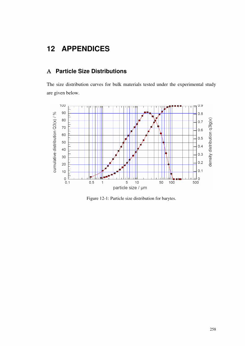
258
12 APPENDICES
���� Particle Size Distributions
The size distribution curves for bulk materials tested under the experimental study
are given below.
Figure 12-1: Particle size distribution for barytes.
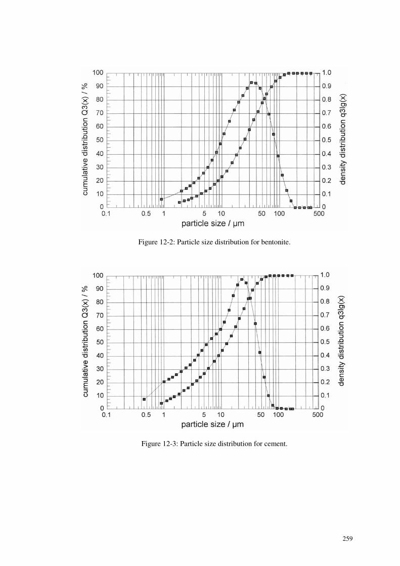
259
Figure 12-2: Particle size distribution for bentonite.
Figure 12-3: Particle size distribution for cement.
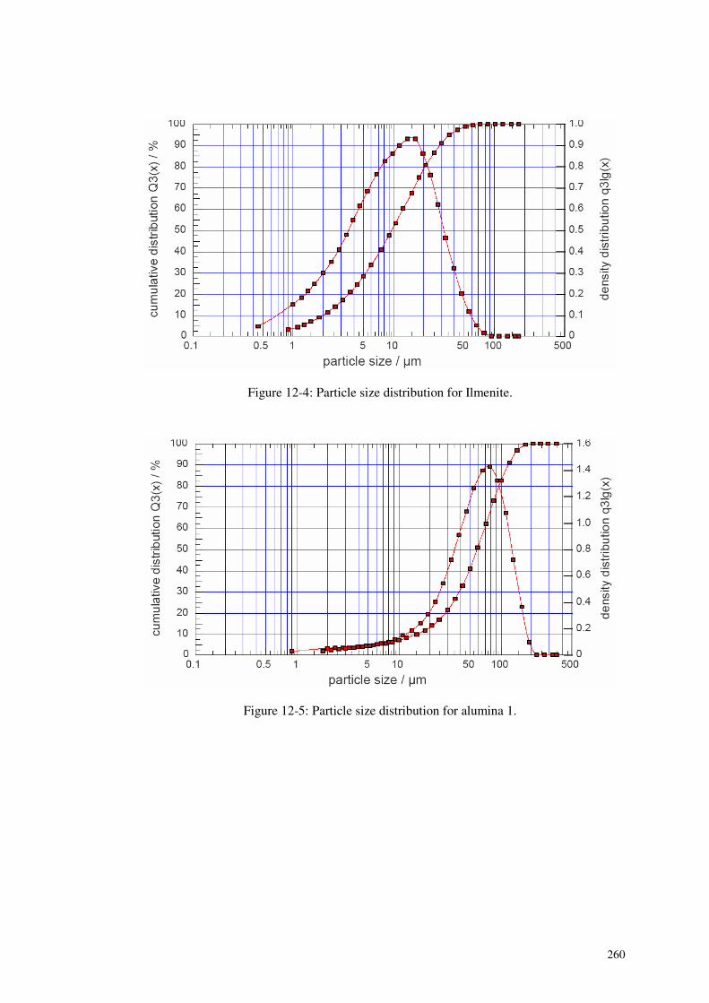
260
Figure 12-4: Particle size distribution for Ilmenite.
Figure 12-5: Particle size distribution for alumina 1.
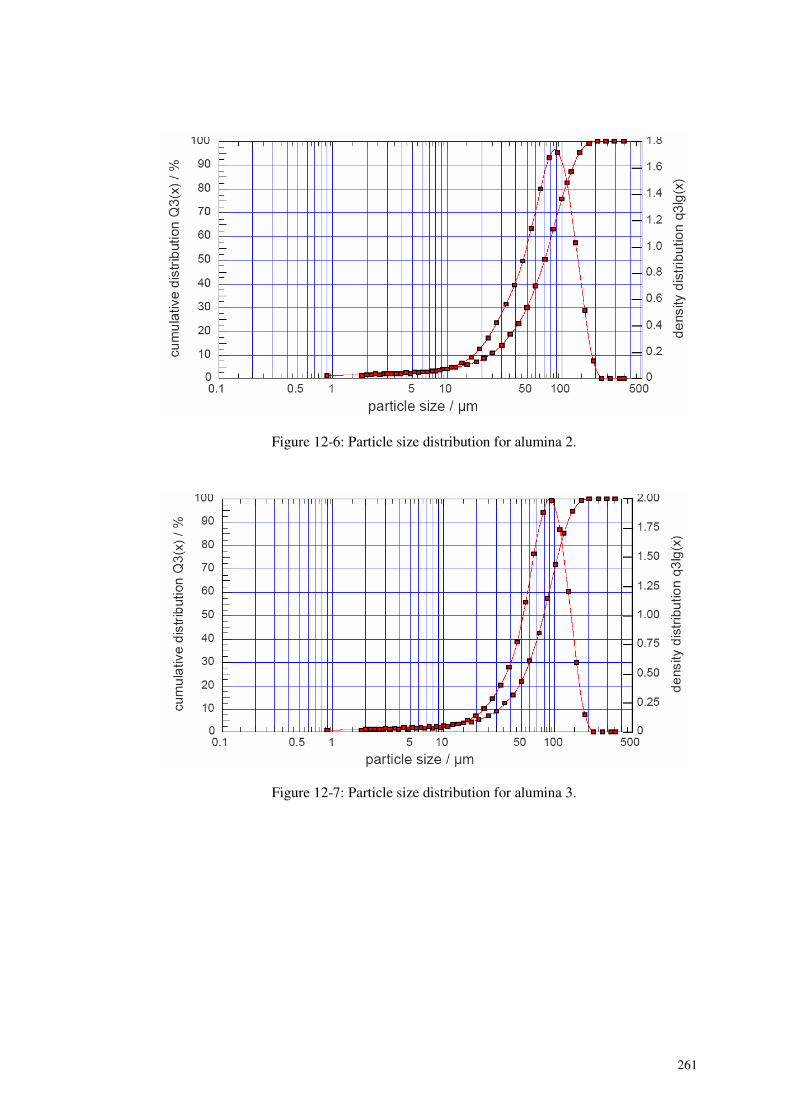
261
Figure 12-6: Particle size distribution for alumina 2.
Figure 12-7: Particle size distribution for alumina 3.
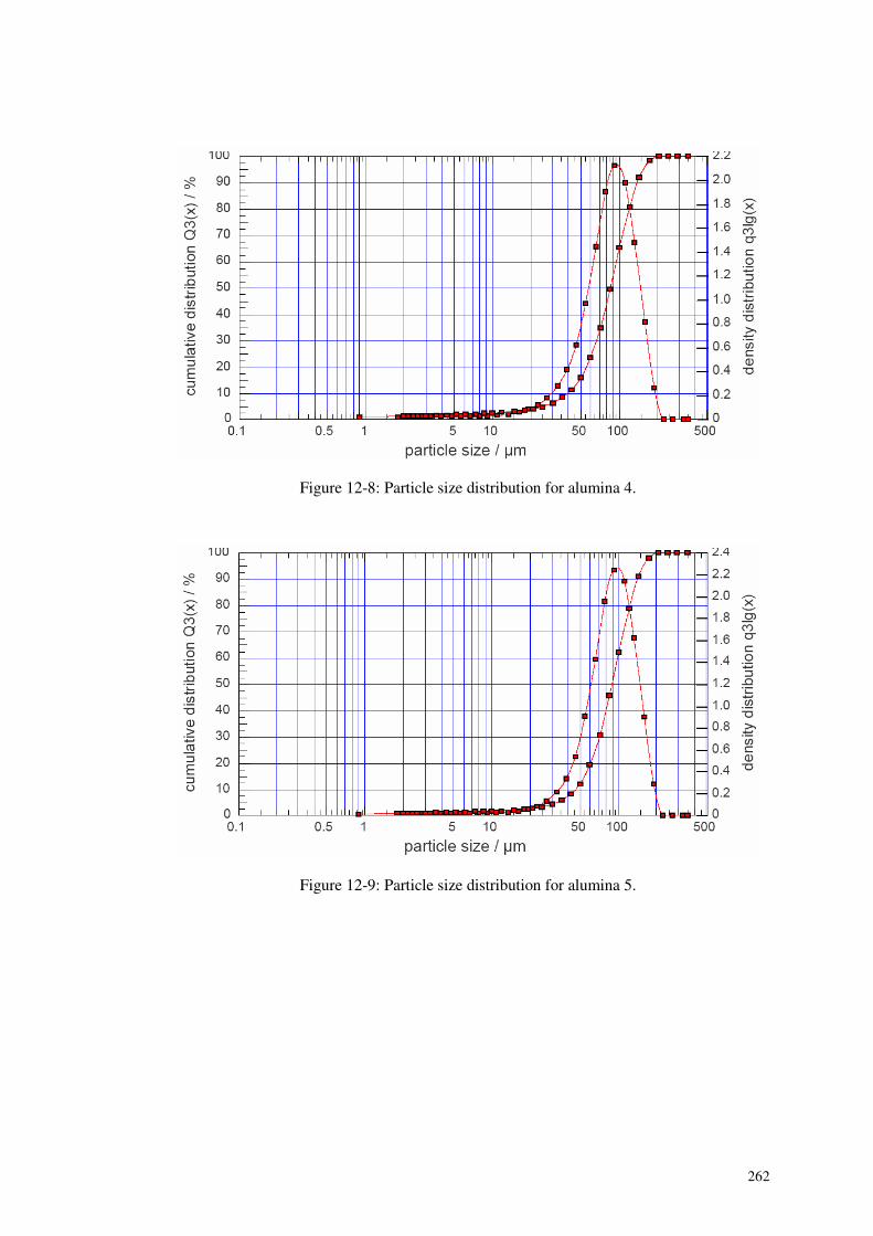
262
Figure 12-8: Particle size distribution for alumina 4.
Figure 12-9: Particle size distribution for alumina 5.
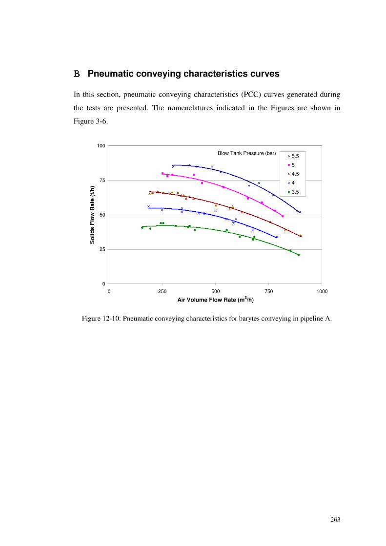
263
���� Pneumatic conveying characteristics curves
In this section, pneumatic conveying characteristics (PCC) curves generated during
the tests are presented. The nomenclatures indicated in the Figures are shown in
Figure 3-6.
0
25
50
75
100
0 250 500 750 1000
Air Volume Flow Rate (m3/h)
So
lids
Flo
wR
ate
(t/h
)
5.5
5
4.5
4
3.5
Blow Tank Pressure (bar)
Figure 12-10: Pneumatic conveying characteristics for barytes conveying in pipeline A.
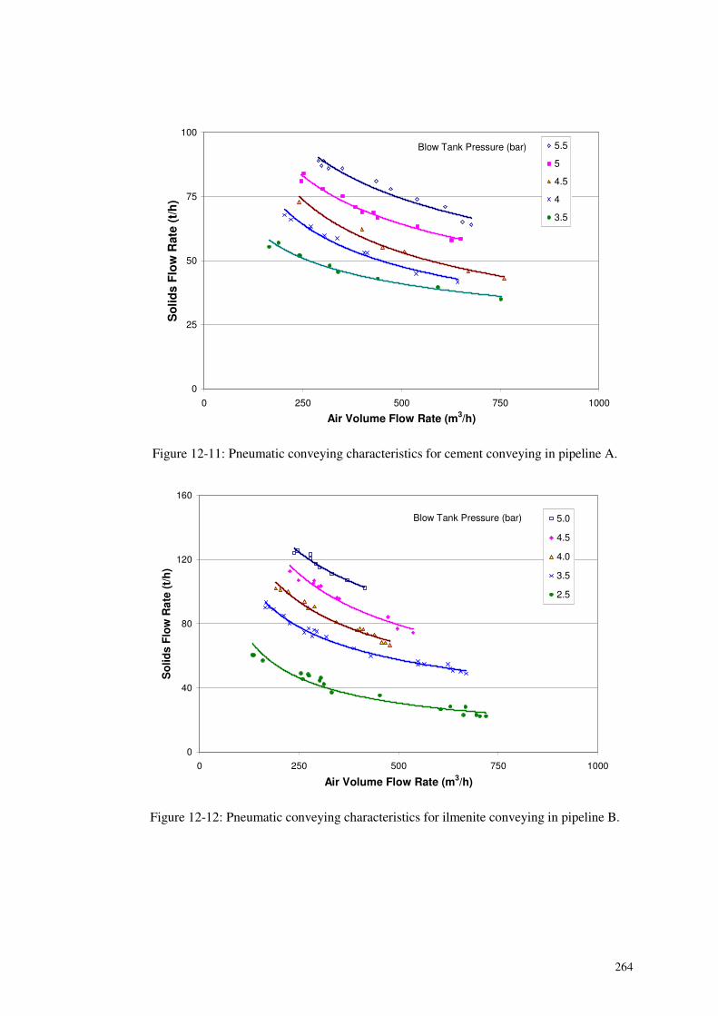
264
0
25
50
75
100
0 250 500 750 1000
Air Volume Flow Rate (m3/h)
So
lids
Flo
wR
ate
(t/h
)
5.5
5
4.5
4
3.5
Blow Tank Pressure (bar)
Figure 12-11: Pneumatic conveying characteristics for cement conveying in pipeline A.
0
40
80
120
160
0 250 500 750 1000
Air Volume Flow Rate (m3/h)
So
lids
Flo
wR
ate
(t/h
)
5.0
4.5
4.0
3.5
2.5
Blow Tank Pressure (bar)
Figure 12-12: Pneumatic conveying characteristics for ilmenite conveying in pipeline B.
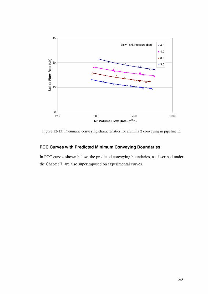
265
0
15
30
45
250 500 750 1000
Air Volume Flow Rate (m3/h)
So
lids
Flo
wR
ate
(t/h
)4.5
4.0
3.5
3.0
Blow Tank Pressure (bar)
Figure 12-13: Pneumatic conveying characteristics for alumina 2 conveying in pipeline E.
PCC Curves with Predicted Minimum Conveying Boundaries
In PCC curves shown below, the predicted conveying boundaries, as described under
the Chapter 7, are also superimposed on experimental curves.
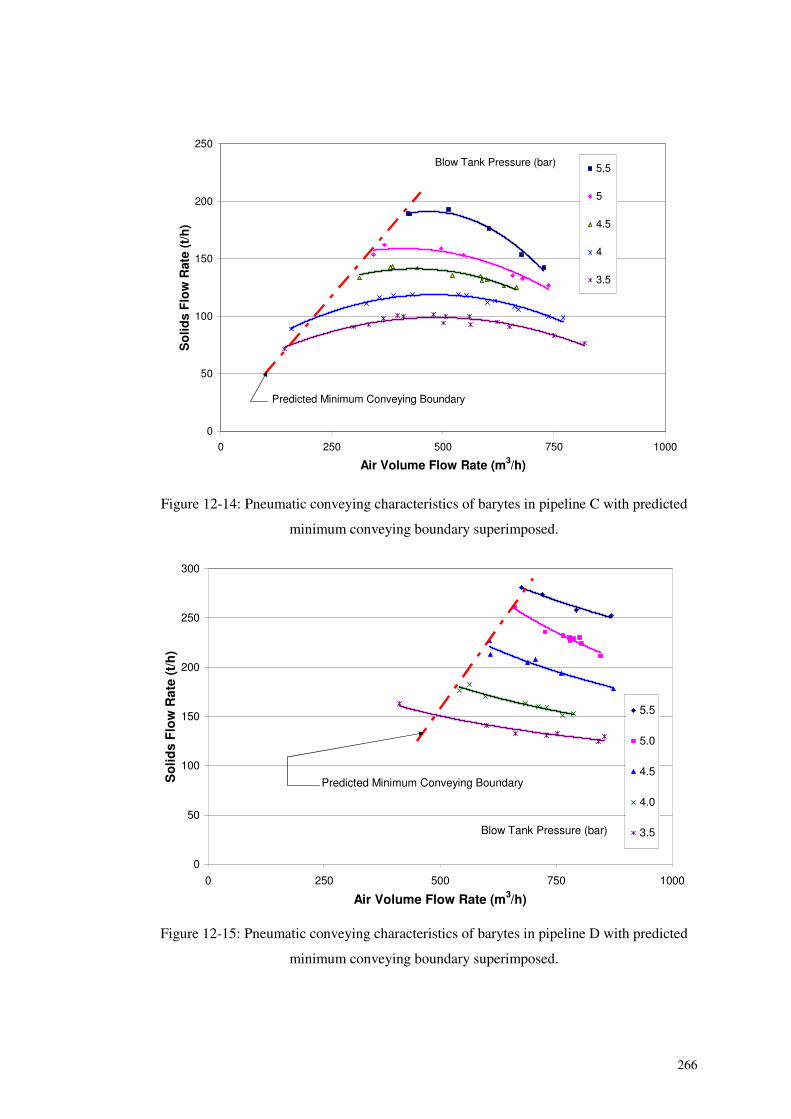
266
0
50
100
150
200
250
0 250 500 750 1000
Air Volume Flow Rate (m3/h)
So
lids
Flo
wR
ate
(t/h
)5,5
5
4.5
4
3.5
Blow Tank Pressure (bar)
Predicted Minimum Conveying Boundary
Figure 12-14: Pneumatic conveying characteristics of barytes in pipeline C with predicted
minimum conveying boundary superimposed.
0
50
100
150
200
250
300
0 250 500 750 1000
Air Volume Flow Rate (m3/h)
So
lids
Flo
wR
ate
(t/h
)
5.5
5.0
4.5
4.0
3.5Blow Tank Pressure (bar)
Predicted Minimum Conveying Boundary
Figure 12-15: Pneumatic conveying characteristics of barytes in pipeline D with predicted
minimum conveying boundary superimposed.
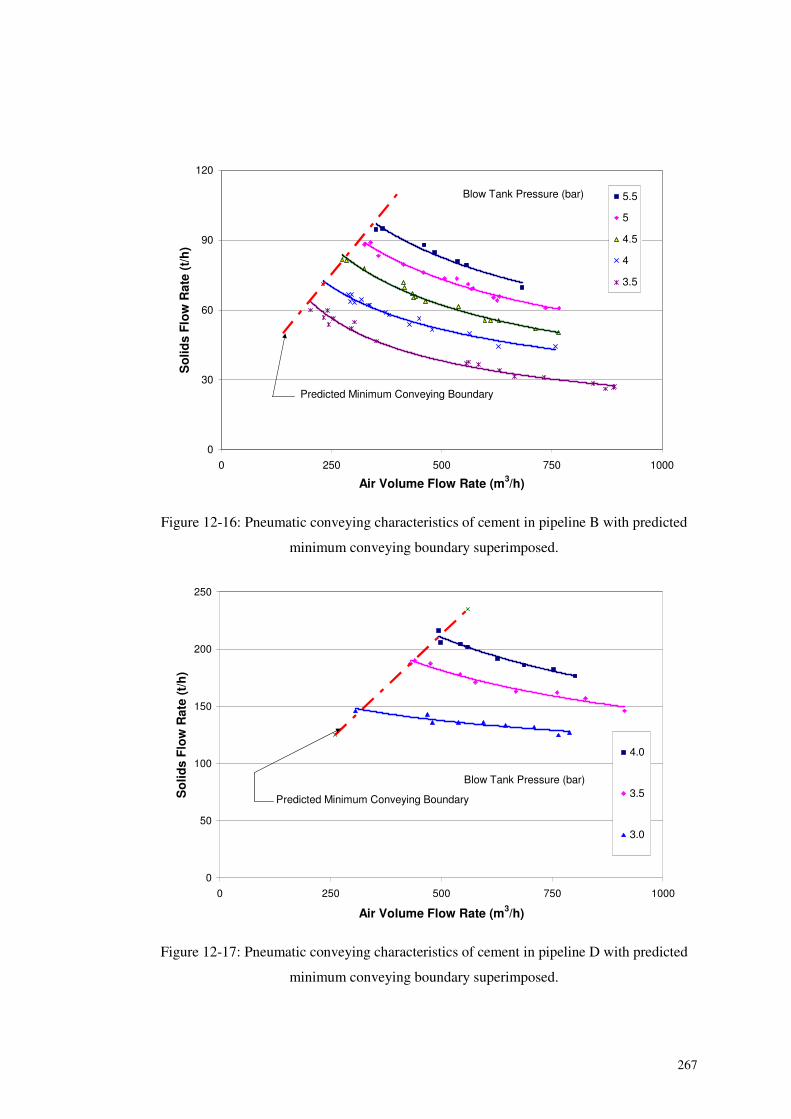
267
0
30
60
90
120
0 250 500 750 1000
Air Volume Flow Rate (m3/h)
So
lids
Flo
wR
ate
(t/h
)5.5
5
4.5
4
3.5
Blow Tank Pressure (bar)
Predicted Minimum Conveying Boundary
Figure 12-16: Pneumatic conveying characteristics of cement in pipeline B with predicted
minimum conveying boundary superimposed.
0
50
100
150
200
250
0 250 500 750 1000
Air Volume Flow Rate (m3/h)
So
lids
Flo
wR
ate
(t/h
)
4.0
3.5
3.0
Blow Tank Pressure (bar)
Predicted Minimum Conveying Boundary
Figure 12-17: Pneumatic conveying characteristics of cement in pipeline D with predicted
minimum conveying boundary superimposed.
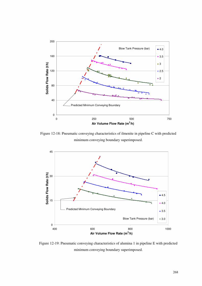
268
0
40
80
120
160
200
0 250 500 750
Air Volume Flow Rate (m3/h)
So
lids
Flo
wR
ate
(t/h
)4.0
3.5
3
2.5
2
Blow Tank Pressure (bar)
Predicted Minimum Conveying Boundary
Figure 12-18: Pneumatic conveying characteristics of ilmenite in pipeline C with predicted
minimum conveying boundary superimposed.
0
15
30
45
400 600 800 1000
Air Volume Flow Rate (m3/h)
So
lids
Flo
wR
ate
(t/h
)
4.5
4.0
3.5
3.0Blow Tank Pressure (bar)
Predicted Minimum Conveying Boundary
Figure 12-19: Pneumatic conveying characteristics of alumina 1 in pipeline E with predicted
minimum conveying boundary superimposed.
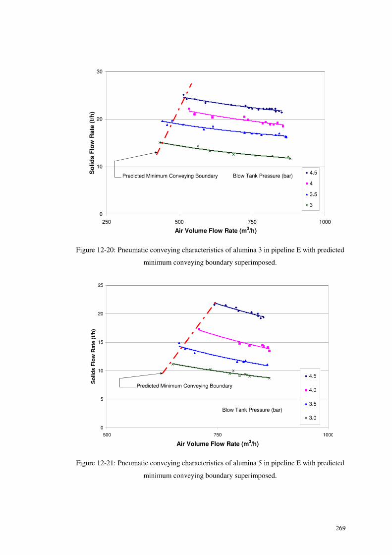
269
0
10
20
30
250 500 750 1000
Air Volume Flow Rate (m3/h)
So
lids
Flo
wR
ate
(t/h
)
4.5
4
3.5
3
Blow Tank Pressure (bar)Predicted Minimum Conveying Boundary
Figure 12-20: Pneumatic conveying characteristics of alumina 3 in pipeline E with predicted
minimum conveying boundary superimposed.
0
5
10
15
20
25
500 750 1000
Air Volume Flow Rate (m3/h)
So
lids
Flo
wR
ate
(t/h
)
4.5
4.0
3.5
3.0
Blow Tank Pressure (bar)
Predicted Minimum Conveying Boundary
Figure 12-21: Pneumatic conveying characteristics of alumina 5 in pipeline E with predicted
minimum conveying boundary superimposed.
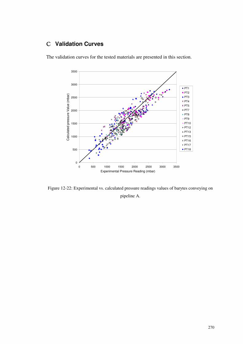
270
���� Validation Curves
The validation curves for the tested materials are presented in this section.
0
500
1000
1500
2000
2500
3000
3500
0 500 1000 1500 2000 2500 3000 3500
Experimental Pressure Reading (mbar)
Cal
cula
ted
pres
sure
Val
ue(m
bar)
PT1
PT2
PT3
PT4
PT5
PT7
PT8
PT9
PT10
PT12
PT13
PT15
PT16
PT17
PT18
Figure 12-22: Experimental vs. calculated pressure readings values of barytes conveying on
pipeline A.
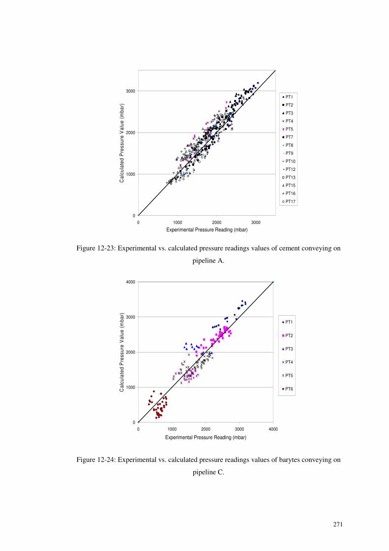
271
0
1000
2000
3000
0 1000 2000 3000
Experimental Pressure Reading (mbar)
Cal
cula
ted
Pre
ssur
eV
alue
(mba
r)
PT1
PT2
PT3
PT4
PT5
PT7
PT8
PT9
PT10
PT12
PT13
PT15
PT16
PT17
Figure 12-23: Experimental vs. calculated pressure readings values of cement conveying on
pipeline A.
0
1000
2000
3000
4000
0 1000 2000 3000 4000
Experimental Pressure Reading (mbar)
Cal
cula
ted
Pre
ssur
eV
alue
(mba
r)
PT1
PT2
PT3
PT4
PT5
PT6
Figure 12-24: Experimental vs. calculated pressure readings values of barytes conveying on
pipeline C.
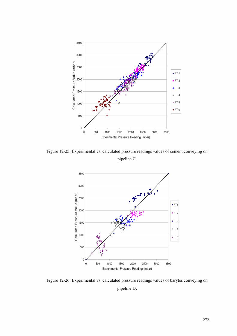
272
0
500
1000
1500
2000
2500
3000
3500
0 500 1000 1500 2000 2500 3000 3500
Experimental Pressure Reading (mbar)
Cal
cula
ted
Pre
ssur
eV
alue
(mba
r)PT 1
PT 2
PT 3
PT 4
PT 5
PT 6
Figure 12-25: Experimental vs. calculated pressure readings values of cement conveying on
pipeline C.
0
500
1000
1500
2000
2500
3000
3500
0 500 1000 1500 2000 2500 3000 3500
Experimental Pressure Reading (mbar)
Cal
cula
ted
Pre
ssur
eV
alue
(mba
r)
PT1
PT2
PT3
PT4
PT5
Figure 12-26: Experimental vs. calculated pressure readings values of barytes conveying on
pipeline D.
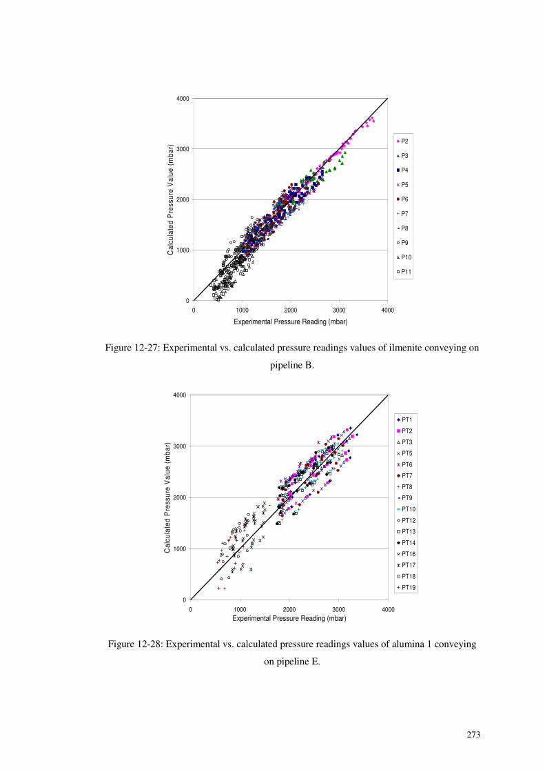
273
0
1000
2000
3000
4000
0 1000 2000 3000 4000
Experimental Pressure Reading (mbar)
Cal
cula
ted
Pre
ssur
eV
alue
(mba
r)
P2
P3
P4
P5
P6
P7
P8
P9
P10
P11
Figure 12-27: Experimental vs. calculated pressure readings values of ilmenite conveying on
pipeline B.
0
1000
2000
3000
4000
0 1000 2000 3000 4000Experimental Pressure Reading (mbar)
Cal
cula
ted
Pre
ssur
eV
alue
(mba
r)
PT1
PT2
PT3
PT5
PT6
PT7
PT8
PT9
PT10
PT12
PT13
PT14
PT16
PT17
PT18
PT19
Figure 12-28: Experimental vs. calculated pressure readings values of alumina 1 conveying
on pipeline E.
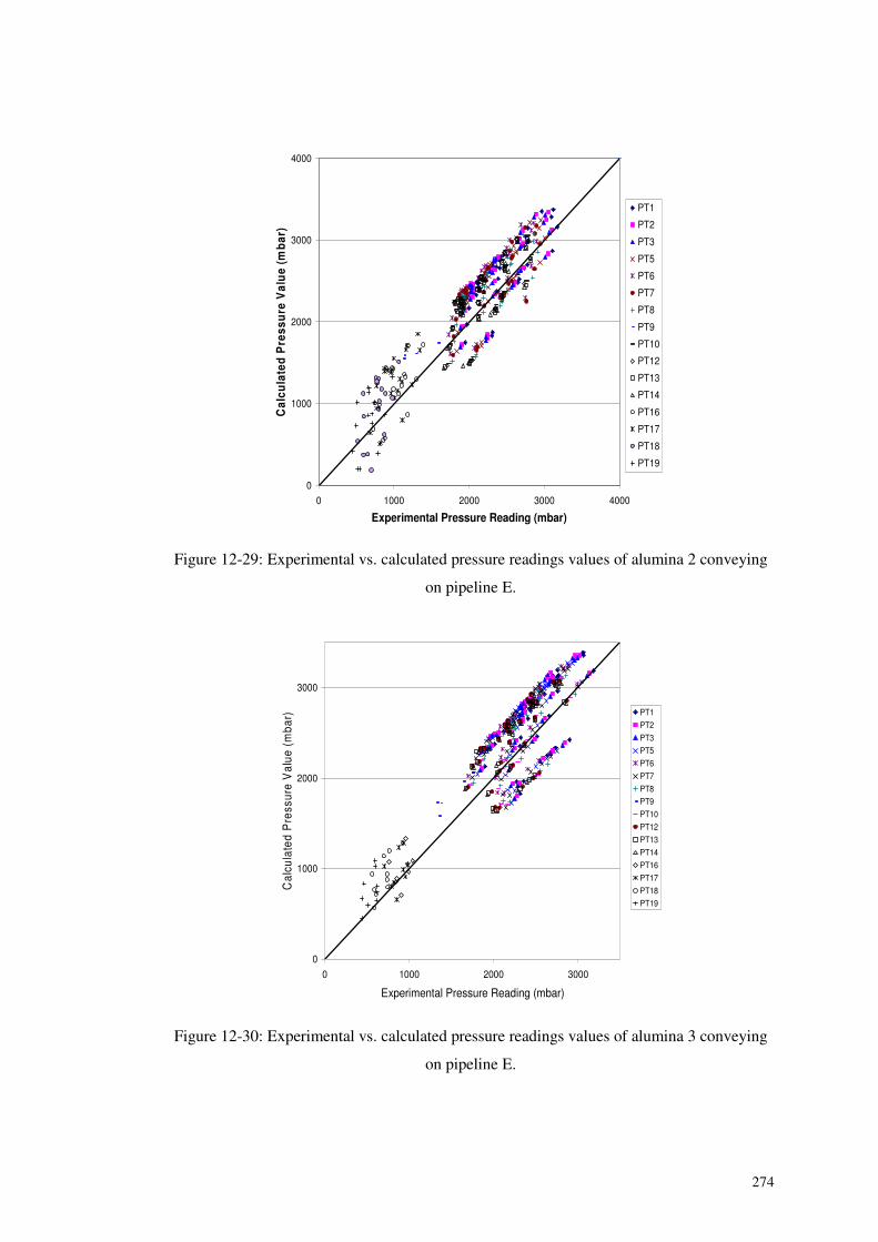
274
0
1000
2000
3000
4000
0 1000 2000 3000 4000
Experimental Pressure Reading (mbar)
Cal
cula
ted
Pre
ssu
reV
alu
e(m
bar)
PT1
PT2
PT3
PT5
PT6
PT7
PT8
PT9
PT10
PT12
PT13
PT14
PT16
PT17
PT18
PT19
Figure 12-29: Experimental vs. calculated pressure readings values of alumina 2 conveying
on pipeline E.
0
1000
2000
3000
0 1000 2000 3000
Experimental Pressure Reading (mbar)
Cal
cula
ted
Pre
ssur
eV
alue
(mba
r) PT1
PT2
PT3
PT5
PT6
PT7
PT8
PT9
PT10
PT12
PT13
PT14
PT16
PT17
PT18
PT19
Figure 12-30: Experimental vs. calculated pressure readings values of alumina 3 conveying
on pipeline E.
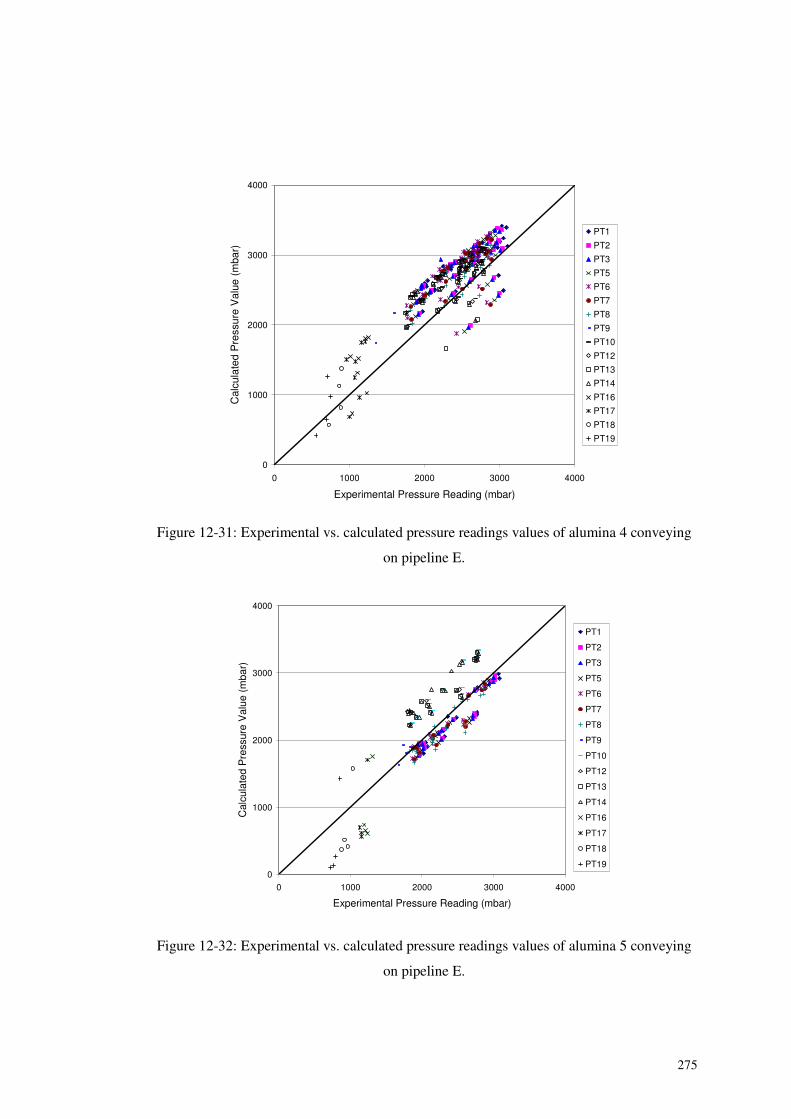
275
0
1000
2000
3000
4000
0 1000 2000 3000 4000
Experimental Pressure Reading (mbar)
Cal
cula
ted
Pre
ssur
eV
alue
(mba
r)PT1
PT2
PT3
PT5
PT6
PT7
PT8
PT9
PT10
PT12
PT13
PT14
PT16
PT17
PT18
PT19
Figure 12-31: Experimental vs. calculated pressure readings values of alumina 4 conveying
on pipeline E.
0
1000
2000
3000
4000
0 1000 2000 3000 4000
Experimental Pressure Reading (mbar)
Cal
cula
ted
Pre
ssur
eV
alue
(mba
r)
PT1
PT2
PT3
PT5
PT6
PT7
PT8
PT9
PT10
PT12
PT13
PT14
PT16
PT17
PT18
PT19
Figure 12-32: Experimental vs. calculated pressure readings values of alumina 5 conveying
on pipeline E.
276
���� List of Publications
International Journal Articles
1. B. K. Datta and C. Ratnayake, A Simple Technique for Scaling Up
Pneumatic Conveying Systems, Particulate Science and Technology, Taylor
& Francis Inc., Vol. 21, No. 3, ISSN: 0272-6351, DOI:
10.1080102726350390223240, pp. 227-236, 2003.
2. B. K. Datta and C. Ratnayake, A. Saasen and Y. Bastesen, A New Design
Approach for Pneumatic Conveying, Annual Transactions of the Nordic
Rheology Society, Vol. 11, 2003, ISSN 1601-4057, pp. 57-62.
3. B. K. Datta, A. Dyroy, C. Ratnayake and M. Karlsen, Influence of Fines
Concentration on Pneumatic Transport Capacity of Alumina, Particulate
Science and Technology, Taylor & Francis Inc., Vol. 21, No. 3, ISSN: 0272-
6351, DOI: 10.1080/02726350390223259, pp. 283-291, 2003.
4. B. K. Datta and C. Ratnayake, A. Saasen and T.H. Omland, Hole Cleaning
and Pressure Loss Prediction from a Bulk Transport Perspective, SPE
International, Society of Petroleum Engineers, SPE 96315, 2005.
5. B.K. Datta and C. Ratnayake, A possible scaling-up technique for dense
phase pneumatic conveying, Particulate Science and Technology, Taylor &
Francis Inc., Vol. 23, No. 2, 2005.
Conference Papers
6. B. K. Datta and C. Ratnayake, A Possible Scaling Up Technique for Dense
Phase Pneumatic Conveying, Proceedings of the 4th International Conference
for Conveying and Handling of Particulate Solids, Budapest, Hungary, May
2003, Vol. 2, pp. 11.74-11.79
7. B. K. Datta and C. Ratnayake, Variation of Pneumatic Transport
Characteristics of Alumina with Change in Size Distribution, Bulk India 2003
- The International Conference and Exhibition for Handling, Processing,
277
Storing and Transporting Bulk Materials, Renaissance Hotel, Mumbai, India,
9 -11 Dec. 2003 (in the electronic format – CD).
8. C. Ratnayake, B. K. Datta, A. Saasen and Y. Bastesen, An Experimental
Study on Entry Pressure Loss in High Pressure Pneumatic Conveying
Systems, Proceedings of 8th International Conference on Bulk Materials
Storage, Handling and Transportation, 2004, Wollongong, Australia, pp.
415-419.
9. C. Ratnayake, M.C. Melaaen and B. K. Datta, An Experimental
Investigation and a CFD Modelling of Gas-solid Flow across a Bend in a
Dense Phase Pneumatic Conveying System, Proceedings of 8th International
Conference on Bulk Materials Storage, Handling and Transportation, 2004,
Wollongong, Australia, pp. 388-393.
10. C. Ratnayake and B.K. Datta, Scaling up of Minimum Conveying
Conditions in a Pneumatic Transport System, Proceedings of 12th
International Conference on Transport & Sedimentation of Solid Particles,
September 2004, Prague, Czech Republic, pp. 565-572.
11. C. Ratnayake, M.C. Melaaen and B. K. Datta, Pressure drop prediction in
dense phase pneumatic conveying using CFD, CFD 2005: 4th International
Conference on CFD in the Oil and Gas, Metallurgical & process industries,
Trondheim, Norway, 6-8 June 2005 (in the electronic format – CD).
Papers Published in Periodicals
12. C. Ratnayake, Experimental Investigation of Scaling Techniques in
Pneumatic Transportation, The POSTEC Newsletter, No. 19, Oct. 2000,
http://www.tel-tek.no/site/content/download/117/446/file/newsletter19.pdf,
pp. 12-13.
13. B. K. Datta and C. Ratnayake, A Step Towards Scaling up Pneumatic
Conveying Systems, The POSTEC Newsletter, No. 21, 2002/2003,
http://www.tel-tek.no/site/content/download/119/452/file/newsletter21.pdf,
pp. 9-11.
278
14. C. Ratnayake, B. K. Datta and M.C. Melaaen, Models for the Scale-up of
Pneumatic Conveying Tests, The POSTEC Newsletter, No. 22, 2004,
http://www.tel-tek.no/site/content/download/634/4969/file/newsletter22.pdf,
pp. 9-10.
15. C. Ratnayake, M.C. Melaaen and B. K. Datta , Pressure Drop Determination
Across a Bend Using CFD, The POSTEC Newsletter, No. 22, 2004,
http://www.tel-tek.no/site/content/download/634/4969/file/newsletter22.pdf,
pp. 11-12.
Papers Communicated for Publication
16. B. K. Datta and C. Ratnayake, An Experimental Study on Degradation of
Maize Starch during Pneumatic Transportation, Communicated to publish in
Particulate Science and Technology, Taylor & Francis Inc.
17. C. Ratnayake, B.K. Datta and M.C. Melaaen, Scale up Technique of Entry
Pressure Loss in Pneumatic Conveying Systems, Communicated to publish in
Particulate Science and Technology, Taylor & Francis Inc.
18. C. Ratnayake, B. K. Datta and M.C. Melaaen, A Unified Scaling-Up
Technique for Pneumatic Conveying Systems, Communicated to publish in
Particulate Science and Technology, Taylor & Francis Inc.
19. C. Ratnayake and B.K. Datta, A Complete Scaling-Up technique for
Designing of Pneumatic Conveying Systems, Accepted for Bulk Days 2005,
Nuremberg, German.
Papers under Preparation
20. C. Ratnayake, B.K. Datta and M.C. Melaaen, An Evaluation of Models
Used for the Pressure Drop Prediction in Pneumatic Conveying
21. C. Ratnayake, M.C. Melaaen and B. K. Datta, A CFD Modelling of Gas-
Solid Flow across a Bend in a Dense Phase Pneumatic Conveying System.
22. C. Ratnayake B.K. Datta and M.C. Melaaen, Comparison Study on
Available Correlations of Minimum Conveying Velocity.

279
23. C. Ratnayake, M.C. Melaaen and B. K. Datta, A CFD Modelling of Gas-
solid Flow across a Straight Section in a Dense Phase Pneumatic Conveying
System.
24. C. Ratnayake, M.C. Melaaen and B. K. Datta, CFD as a Pressure Drop
Prediciton Tool in a Dense Phase Pneumatic Conveying System.